Moscow Institute of Physics and Technology

and

P.N.Lebedev Physical Institute

Professor Nikolai Kolachevsky

Precision measurements

in quantum optics

Lecture scripts supplementary

The goal of the lecture course is to deliver modern experimental and the-oretical methods of precision measurements in quantum optics. The mainobjectives of the course are the following

• description of stochastic processes in oscillatory systems

• discussion of precision methods in astrophysics and space, introductionto General relativity

• detailed presentation of modern methods of laser cooling, discussion ofdifferent trapping methods of atoms and ions

• discussion of modern approaches to laser stabilization and optical fre-quency measurements, optical clocks

Moscow, Russia, 2013

Contents

Lecture 1 51.1 Frequency and time as most accurately measured quantities in

physics . . . . . . . . . . . . . . . . . . . . . . . . . . . . . . . . 51.2 Clocks: from 17th century till today. . . . . . . . . . . . . . . . 6

1.2.1 Mechanical clocks . . . . . . . . . . . . . . . . . . . . . . 61.2.2 Quartz clocks . . . . . . . . . . . . . . . . . . . . . . . . 71.2.3 Microwave atomic clocks . . . . . . . . . . . . . . . . . . 71.2.4 Optical clocks . . . . . . . . . . . . . . . . . . . . . . . . 81.2.5 Accuracy and stability: definition . . . . . . . . . . . . . 9

1.3 Oscillator. Amplitude and Phase modulation . . . . . . . . . . . 91.3.1 Harmonic oscillator . . . . . . . . . . . . . . . . . . . . . 91.3.2 Damped oscillations . . . . . . . . . . . . . . . . . . . . 101.3.3 Harmonic amplitude modulation . . . . . . . . . . . . . . 121.3.4 Harmonic phase modulation . . . . . . . . . . . . . . . . 13

Lecture 2: Amplitude and phase fluctuations 182.1 Mathematical description of stochastic processes, distribution

function, mean value, dispersion. . . . . . . . . . . . . . . . . . 182.2 Allan deviation. . . . . . . . . . . . . . . . . . . . . . . . . . . . 20

2.2.1 Correlated fluctuations . . . . . . . . . . . . . . . . . . . 232.3 Spectral representation of frequency fluctuations . . . . . . . . . 252.4 From spectral representation of fluctuations to time represen-

tation . . . . . . . . . . . . . . . . . . . . . . . . . . . . . . . . 29

Lecture 3: From frequency fluctuations to spectral line shape 333.1 Power spectral density of a quasimonochromatic signal with a

fluctuating phase. . . . . . . . . . . . . . . . . . . . . . . . . . . 333.1.1 Spectrum with shallow high-frequency fluctuations . . . 353.1.2 Spectrum with slow and deep frequency fluctuations . . . 373.1.3 Spectrum with a weak phase noise . . . . . . . . . . . . 383.1.4 Spectrum with phase noise: power in the carrier and

carrier collapse . . . . . . . . . . . . . . . . . . . . . . . 393.2 Measurement methods . . . . . . . . . . . . . . . . . . . . . . . 40

2

3.2.1 Heterodyne measurements . . . . . . . . . . . . . . . . . 41

Lecture 4: General relativity in applications to time and fre-quency transfer 454.1 Basics of General Relativity . . . . . . . . . . . . . . . . . . . . 464.2 Transformation of time: gravitational shift, time dilation, Sagnac

effect . . . . . . . . . . . . . . . . . . . . . . . . . . . . . . . . . 484.3 Time and frequency comparison . . . . . . . . . . . . . . . . . . 51

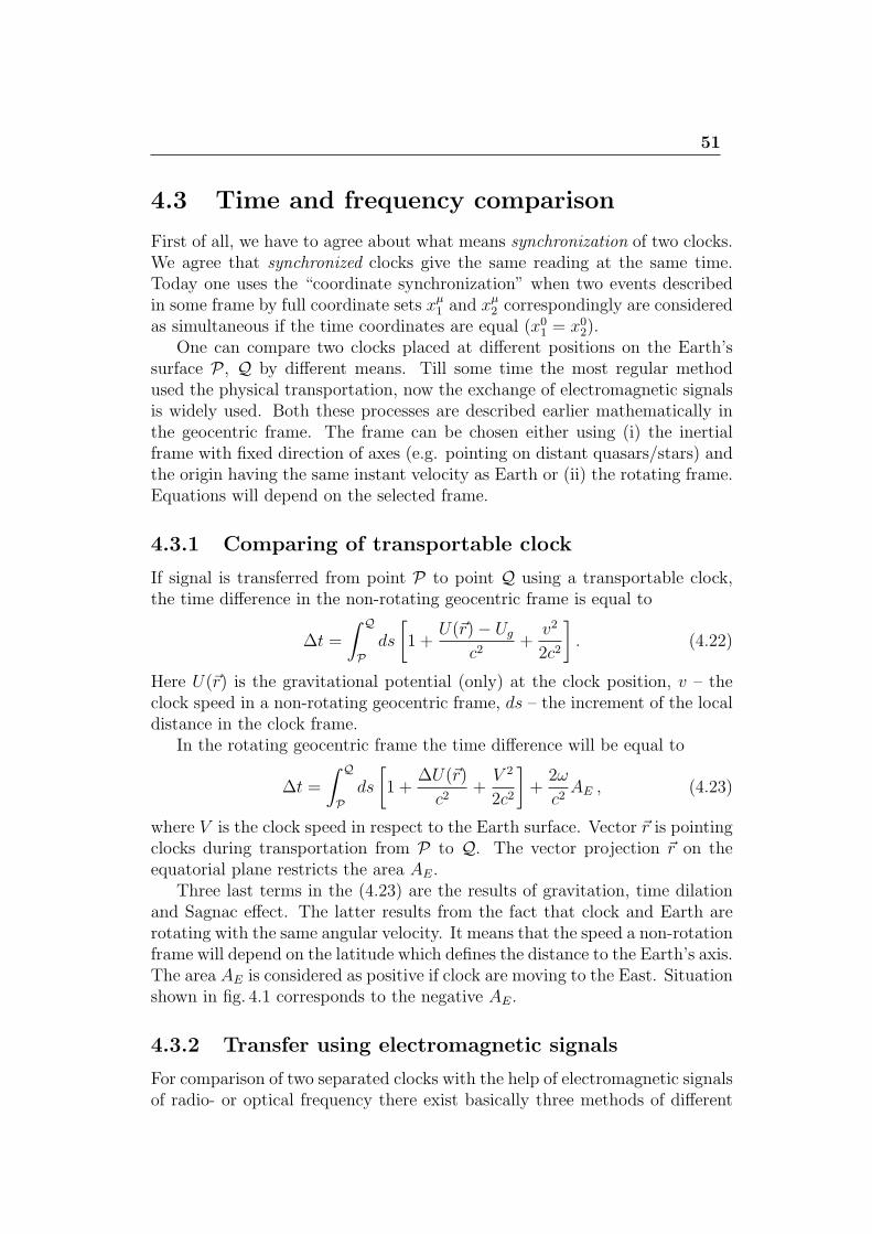
4.3.1 Comparing of transportable clock . . . . . . . . . . . . . 514.3.2 Transfer using electromagnetic signals . . . . . . . . . . . 514.3.3 Transfer of optical frequencies . . . . . . . . . . . . . . . 54

Lecture 5: Introduction to Global navigation systems 555.1 Global navigation system . . . . . . . . . . . . . . . . . . . . . . 55

5.1.1 Principles of satellite navigation . . . . . . . . . . . . . . 555.1.2 GPS system operation . . . . . . . . . . . . . . . . . . . 56

5.2 Code division multiplexing (Synchronous CDMA) . . . . . . . . 655.2.1 Example . . . . . . . . . . . . . . . . . . . . . . . . . . . 665.2.2 Asynchronous CDMA . . . . . . . . . . . . . . . . . . . 675.2.3 Flexible allocation of resources . . . . . . . . . . . . . . . 685.2.4 Spread-spectrum characteristics of CDMA . . . . . . . . 69

Lecture 6: Precision measurements in astrophysics 706.1 Pulsars and Frequency Standards . . . . . . . . . . . . . . . . . 70

6.1.1 Pulsar chronometry . . . . . . . . . . . . . . . . . . . . . 736.2 Binary pulsars . . . . . . . . . . . . . . . . . . . . . . . . . . . . 746.3 White dwarfs . . . . . . . . . . . . . . . . . . . . . . . . . . . . 766.4 Introduction to gravitational waves . . . . . . . . . . . . . . . . 78

6.4.1 Very Large Baseline Interferometry . . . . . . . . . . . . 806.5 Search for drift of the fine structure constant . . . . . . . . . . . 81

Lecture 7: Two levels atomic system and frequency standards 827.1 Two-level system . . . . . . . . . . . . . . . . . . . . . . . . . . 827.2 Optical Bloch equations . . . . . . . . . . . . . . . . . . . . . . 837.3 Ramsey method . . . . . . . . . . . . . . . . . . . . . . . . . . . 88

7.3.1 Bloch sphere representation . . . . . . . . . . . . . . . . 897.3.2 Spectral representation . . . . . . . . . . . . . . . . . . . 917.3.3 Atomic interferometry . . . . . . . . . . . . . . . . . . . 91

7.4 Microwave frequency standards . . . . . . . . . . . . . . . . . . 927.4.1 Cesium beam clock . . . . . . . . . . . . . . . . . . . . . 927.4.2 Cs fountain clock . . . . . . . . . . . . . . . . . . . . . . 937.4.3 Stability of Cs clocks . . . . . . . . . . . . . . . . . . . . 95

3

Lecture 8: Laser cooling of atoms 968.1 Optical molasses . . . . . . . . . . . . . . . . . . . . . . . . . . 978.2 The Doppler limit . . . . . . . . . . . . . . . . . . . . . . . . . . 998.3 Subdoppler cooling . . . . . . . . . . . . . . . . . . . . . . . . . 100

Lecture 9: Traps for neutral atoms 1039.1 Magnetic dipole trap . . . . . . . . . . . . . . . . . . . . . . . . 1049.2 Optical dipole trap . . . . . . . . . . . . . . . . . . . . . . . . . 1069.3 Magneto-optical trap . . . . . . . . . . . . . . . . . . . . . . . . 1089.4 Optical lattice . . . . . . . . . . . . . . . . . . . . . . . . . . . . 111

Lecture 10: Paul trap for ions 11310.1 Traps for charged particles . . . . . . . . . . . . . . . . . . . . . 11310.2 Paul trap . . . . . . . . . . . . . . . . . . . . . . . . . . . . . . 11410.3 Linear quadrupole trap . . . . . . . . . . . . . . . . . . . . . . . 11410.4 Mathieu equations . . . . . . . . . . . . . . . . . . . . . . . . . 11610.5 Pseudopotential . . . . . . . . . . . . . . . . . . . . . . . . . . . 11810.6 Three-dimensional Paul trap. . . . . . . . . . . . . . . . . . . . 120

Lecture 11: Penning trap for ions and ion cooling 12211.1 Penning trap . . . . . . . . . . . . . . . . . . . . . . . . . . . . 122

11.1.1 Rigorous solution . . . . . . . . . . . . . . . . . . . . . . 12411.1.2 Ion energies in the Penning trap. . . . . . . . . . . . . . 12411.1.3 Interactions between trapped ions . . . . . . . . . . . . . 125

11.2 Lamb-Dicke regime . . . . . . . . . . . . . . . . . . . . . . . . . 12611.3 Trap loading . . . . . . . . . . . . . . . . . . . . . . . . . . . . . 12711.4 Ion cooling . . . . . . . . . . . . . . . . . . . . . . . . . . . . . . 127

11.4.1 Energy dissipation by an electric circuit . . . . . . . . . 12811.4.2 Buffer gas cooling . . . . . . . . . . . . . . . . . . . . . . 12811.4.3 Doppler laser cooling . . . . . . . . . . . . . . . . . . . . 129

11.5 Detection of trapped ions . . . . . . . . . . . . . . . . . . . . . . 13111.5.1 Optical registration . . . . . . . . . . . . . . . . . . . . . 131

Lecture 12: Methods of quantum logic in optical clocks 13212.1 Electron shelving . . . . . . . . . . . . . . . . . . . . . . . . . . 13312.2 Elements of quantum logic in ion traps . . . . . . . . . . . . . . 13412.3 Implementation of Cirac-Zoller gate . . . . . . . . . . . . . . . . 136

12.3.1 States of an ion . . . . . . . . . . . . . . . . . . . . . . . 13612.3.2 2π rotation of the spin-1/2 system . . . . . . . . . . . . . 13612.3.3 Collective vibrational modes . . . . . . . . . . . . . . . . 13812.3.4 CNOT gate . . . . . . . . . . . . . . . . . . . . . . . . . 138

12.4 Information transfer between clock and cooling ions. Precisionspectroscopy using quantum logic. . . . . . . . . . . . . . . . . . 140

4

Lecture 13: Optical frequency measurements 14313.1 Introduction to some optical non-linear processes . . . . . . . . 14413.2 Ultrashort pulses and femtosecond laser basics . . . . . . . . . . 14513.3 EOM as the frequency shifting element . . . . . . . . . . . . . . 146

13.3.1 EOM for the frequency comb synthesis . . . . . . . . . . 14713.4 Kerr mode-locking . . . . . . . . . . . . . . . . . . . . . . . . . 147

13.4.1 Propagation of ultra short pulses . . . . . . . . . . . . . 14813.5 Precision optical spectroscopy and optical frequency measure-

ments . . . . . . . . . . . . . . . . . . . . . . . . . . . . . . . . 14913.5.1 Ultra-short pulse lasers and frequency combs . . . . . . . 150

Lecture 1: Introduction

Frequency and time as most accurately measured quantities in physics. Clocks:from 17th century till today. Mechanical, radiofrequency, microwave and opti-cal oscillators. Accuracy and stability. Phase and amplitude modulation, theirmathematical representation and power spectrum.

1.1 Frequency and time as most accurately

measured quantities in physics

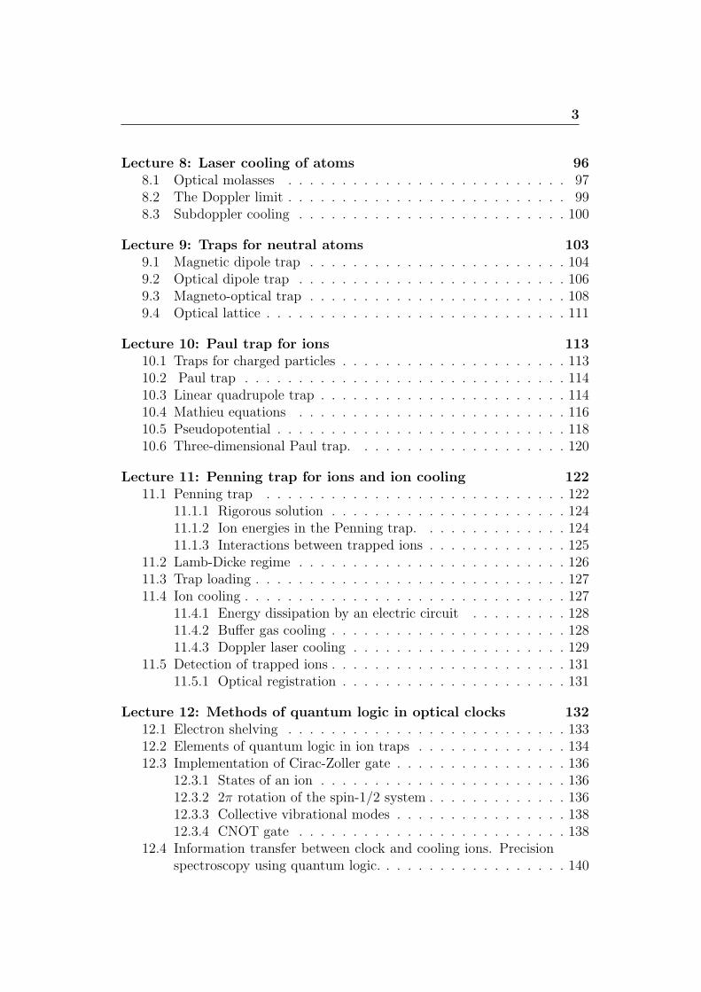
Figure 1.1: Typical frequencies of different oscillator types.

From all known physical quantities, frequency can be measured with thehighest accuracy. Today, the accuracy of the frequency measurements reacheda few parts in 1018. If someone wants to measure a physical quantity with highaccuracy, it is necessary to covert this quantity in frequency.

Examples:- road radars convert velocity into frequency (the Doppler effect)- medical tomograph maps the spatial distribution of water containing tissuesinto frequency spectrum (Nuclear Magnetic Resonance)- highly accurate measurements of voltages use the Josephson effect: the os-cillation frequency from the Josephson junction depends on the potential dif-ference as UDC = n h

2eω.

For many applications in our life, technology, navigation and fundamentalphysics stable frequency sources are extremely important. Humans used clocks

6

from the very beginning of civilization.First clocks were based on periodicity of day and night and changing sea-

sons. It is directly connected to the rotation of astronomical bodies - Earth,Moon and planets. The rotation period of the Earth around its axis (day),Moon around the Earth (month) and Earth around the Sun (year) were takenas natural units of time. One needs the time scale and the unit of time todiscuss events happening our life.

Today the tropical year consists of 365.2422 days and the synodic month –of 29.5306 days. Today’s calender bases on Julian (roman) calender acceptedin 45 B.C.: the year consists of 365 days, while each 4th year consists of 366days. The calender was slightly modified in 1582 by pope Gregory. Accordingto this calender the year consists of 365.2425 days which is very close to truenumber (365.2422 days).

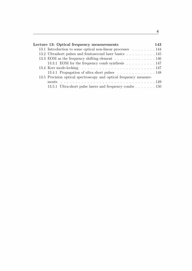
1.2 Clocks: from 17th century till today.

Figure 1.2: Development of clocks over last centuries.

1.2.1 Mechanical clocks

In mechanical clocks the mechanism plays a dual role. It should measure andindicate the frequency of the oscillating system. In addition, it should provideenergy to compensate for the losses in the system. It should not influence thefrequency of the oscillator! First tower clocks had an accuracy of 15 minutesin a day or ∆T/T = ∆ν/ν ≈ 10−2.

7

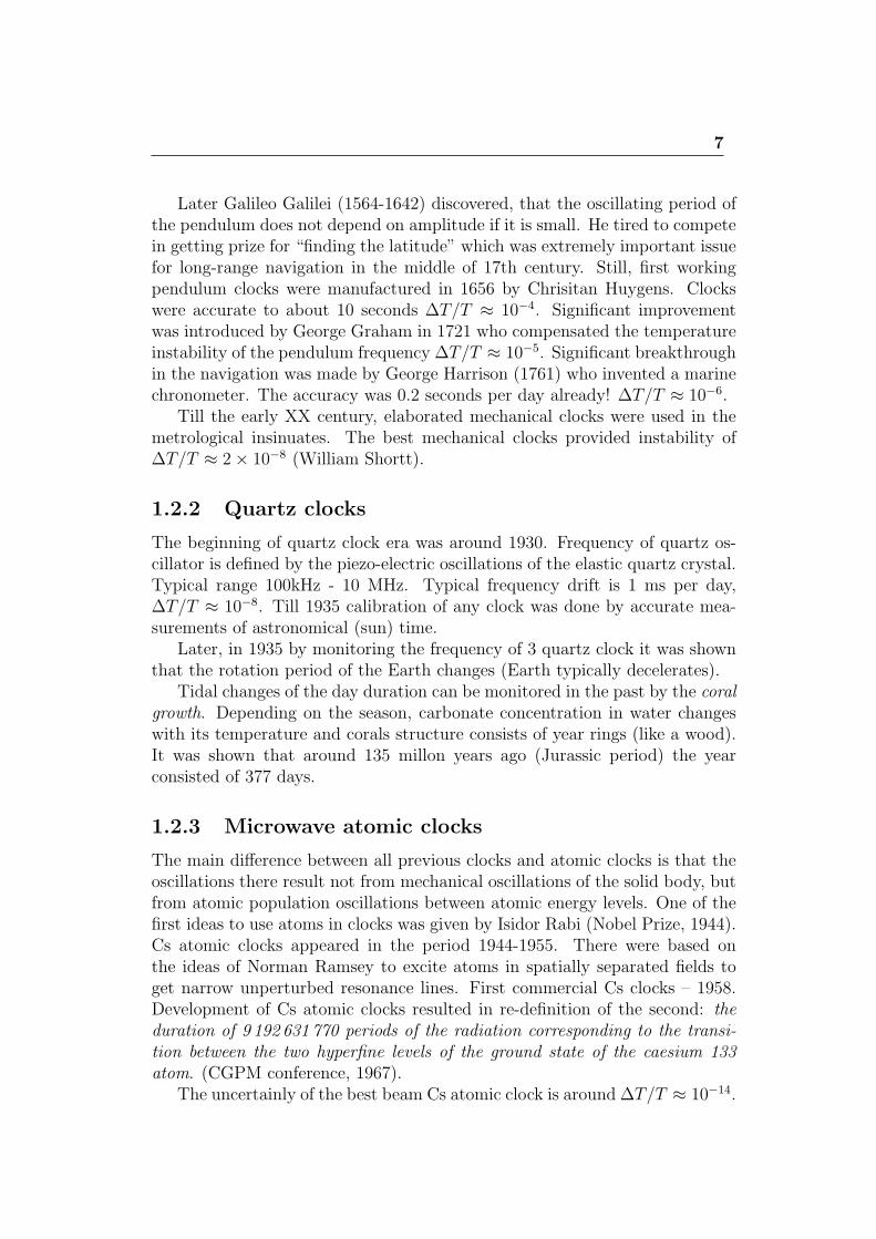
Later Galileo Galilei (1564-1642) discovered, that the oscillating period ofthe pendulum does not depend on amplitude if it is small. He tired to competein getting prize for “finding the latitude” which was extremely important issuefor long-range navigation in the middle of 17th century. Still, first workingpendulum clocks were manufactured in 1656 by Chrisitan Huygens. Clockswere accurate to about 10 seconds ∆T/T ≈ 10−4. Significant improvementwas introduced by George Graham in 1721 who compensated the temperatureinstability of the pendulum frequency ∆T/T ≈ 10−5. Significant breakthroughin the navigation was made by George Harrison (1761) who invented a marinechronometer. The accuracy was 0.2 seconds per day already! ∆T/T ≈ 10−6.

Till the early XX century, elaborated mechanical clocks were used in themetrological insinuates. The best mechanical clocks provided instability of∆T/T ≈ 2× 10−8 (William Shortt).

1.2.2 Quartz clocks

The beginning of quartz clock era was around 1930. Frequency of quartz os-cillator is defined by the piezo-electric oscillations of the elastic quartz crystal.Typical range 100kHz - 10 MHz. Typical frequency drift is 1 ms per day,∆T/T ≈ 10−8. Till 1935 calibration of any clock was done by accurate mea-surements of astronomical (sun) time.

Later, in 1935 by monitoring the frequency of 3 quartz clock it was shownthat the rotation period of the Earth changes (Earth typically decelerates).

Tidal changes of the day duration can be monitored in the past by the coralgrowth. Depending on the season, carbonate concentration in water changeswith its temperature and corals structure consists of year rings (like a wood).It was shown that around 135 millon years ago (Jurassic period) the yearconsisted of 377 days.

1.2.3 Microwave atomic clocks

The main difference between all previous clocks and atomic clocks is that theoscillations there result not from mechanical oscillations of the solid body, butfrom atomic population oscillations between atomic energy levels. One of thefirst ideas to use atoms in clocks was given by Isidor Rabi (Nobel Prize, 1944).Cs atomic clocks appeared in the period 1944-1955. There were based onthe ideas of Norman Ramsey to excite atoms in spatially separated fields toget narrow unperturbed resonance lines. First commercial Cs clocks – 1958.Development of Cs atomic clocks resulted in re-definition of the second: theduration of 9 192 631 770 periods of the radiation corresponding to the transi-tion between the two hyperfine levels of the ground state of the caesium 133atom. (CGPM conference, 1967).

The uncertainly of the best beam Cs atomic clock is around ∆T/T ≈ 10−14.

8

Next generation of microwave Cs atomic clocks - “Cs fountain clocks”.Atoms are laser cooled and set to ballistic flight for 1 s. It results in spectralline width of the atomic resonance line of 1 Hz. The typical uncertainty is∆T/T ≈ 10−15, the best performance ∆T/T = 2− 3× 10−16.

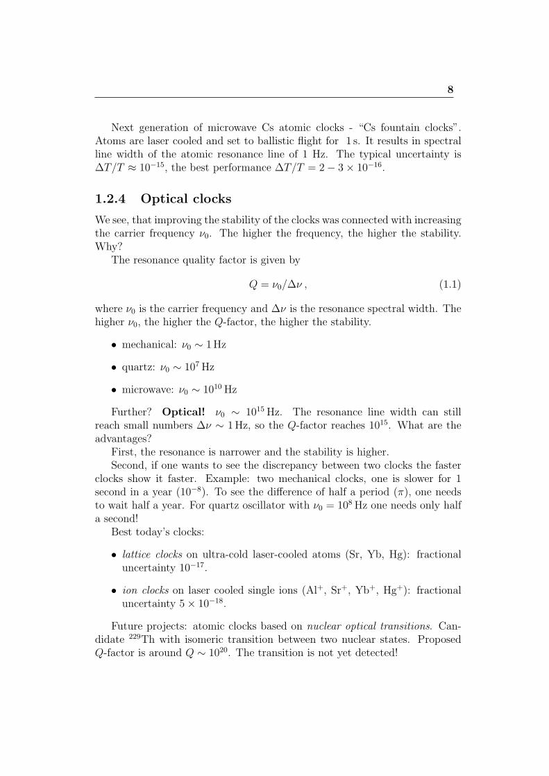
1.2.4 Optical clocks

We see, that improving the stability of the clocks was connected with increasingthe carrier frequency ν0. The higher the frequency, the higher the stability.Why?

The resonance quality factor is given by

Q = ν0/∆ν , (1.1)

where ν0 is the carrier frequency and ∆ν is the resonance spectral width. Thehigher ν0, the higher the Q-factor, the higher the stability.

• mechanical: ν0 ∼ 1Hz

• quartz: ν0 ∼ 107Hz

• microwave: ν0 ∼ 1010Hz

Further? Optical! ν0 ∼ 1015Hz. The resonance line width can stillreach small numbers ∆ν ∼ 1Hz, so the Q-factor reaches 1015. What are theadvantages?

First, the resonance is narrower and the stability is higher.Second, if one wants to see the discrepancy between two clocks the faster

clocks show it faster. Example: two mechanical clocks, one is slower for 1second in a year (10−8). To see the difference of half a period (π), one needsto wait half a year. For quartz oscillator with ν0 = 108Hz one needs only halfa second!

Best today’s clocks:

• lattice clocks on ultra-cold laser-cooled atoms (Sr, Yb, Hg): fractionaluncertainty 10−17.

• ion clocks on laser cooled single ions (Al+, Sr+, Yb+, Hg+): fractionaluncertainty 5× 10−18.

Future projects: atomic clocks based on nuclear optical transitions. Can-didate 229Th with isomeric transition between two nuclear states. ProposedQ-factor is around Q ∼ 1020. The transition is not yet detected!

9

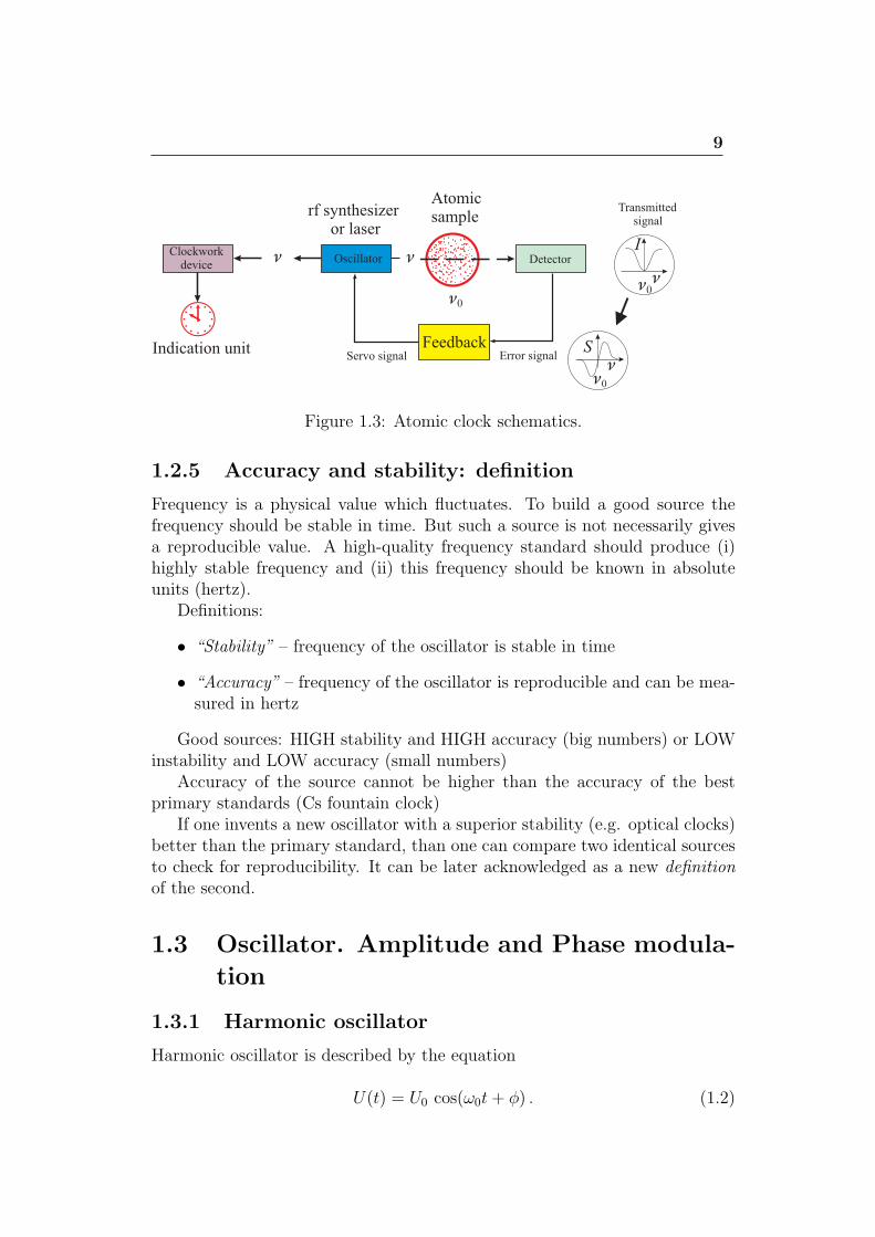
Figure 1.3: Atomic clock schematics.

1.2.5 Accuracy and stability: definition

Frequency is a physical value which fluctuates. To build a good source thefrequency should be stable in time. But such a source is not necessarily givesa reproducible value. A high-quality frequency standard should produce (i)highly stable frequency and (ii) this frequency should be known in absoluteunits (hertz).

Definitions:

• “Stability” – frequency of the oscillator is stable in time

• “Accuracy” – frequency of the oscillator is reproducible and can be mea-sured in hertz

Good sources: HIGH stability and HIGH accuracy (big numbers) or LOWinstability and LOW accuracy (small numbers)

Accuracy of the source cannot be higher than the accuracy of the bestprimary standards (Cs fountain clock)

If one invents a new oscillator with a superior stability (e.g. optical clocks)better than the primary standard, than one can compare two identical sourcesto check for reproducibility. It can be later acknowledged as a new definitionof the second.

1.3 Oscillator. Amplitude and Phase modula-

tion

1.3.1 Harmonic oscillator

Harmonic oscillator is described by the equation

U(t) = U0 cos(ω0t+ ϕ) . (1.2)

10

Figure 1.4: Accuracy and stability. a) Accurate and stable signal. b) Accurateand unstable signal. c) Stable, but not accurate signal.

with the amplitude U0, frequency

ν0 =ω0

2π(1.3)

and initial phase ϕ.Let us generalize the equation for harmonic oscillations introducing varying

phase and amplitude:

U(t) = U0(t) cosφ(t) = [U0 +∆U0(t)] cos[ω0t+ ϕ(t)]. (1.4)

instant frequency equals

ν(t) ≡ 1

2π

dφ(t)

dt=

1

2π

d

dt[2πν0t+ ϕ(t)] = ν0 +

1

2π

dϕ(t)

dt(1.5)

which differs from the frequency of the ideal oscillator ν0 by

∆ν(t) ≡ 1

2π

dϕ(t)

dt. (1.6)

1.3.2 Damped oscillations

Damped oscillations are described by the formula

U(t) = U0 e−Γ

2t cosω0t , (1.7)

where Γ is the damping constant. It is defined by the energy losses of the oscil-lator per unit time dW (t) = −ΓW (t) dt. The spectrum of damping oscillationsis given by Fourier transformation

A(ω) =

∫ ∞

0

U0 e−Γ

2t cos(ω0t) e

−iωt dt , (1.8)

11

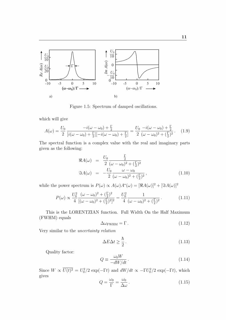
Figure 1.5: Spectrum of damped oscillations.

which will give

A(ω) =U0

2

−i(ω − ω0) +Γ2

[i(ω − ω0) +Γ2][−i(ω − ω0) +

Γ2]=U0

2

−i(ω − ω0) +Γ2

(ω − ω0)2 + (Γ2)2. (1.9)

The spectral function is a complex value with the real and imaginary partsgiven as the following:

ℜA(ω) =U0

2

Γ2

(ω − ω0)2 + (Γ2)2

ℑA(ω) = −U0

2

ω − ω0

(ω − ω0)2 + (Γ2)2, (1.10)

while the power spectrum is P (ω) ∝ A(ω)A∗(ω) = [ℜA(ω)]2 + [ℑA(ω)]2

P (ω) ∝ U20

4

(ω − ω0)2 + (Γ

2)2

[(ω − ω0)2 + (Γ2)2]2

=U20

4

1

(ω − ω0)2 + (Γ2)2. (1.11)

This is the LORENTZIAN function. Full Width On the Half Maximum(FWHM) equals

∆ωFWHM = Γ . (1.12)

Very similar to the uncertainty relation

∆E∆t ≥ h

2. (1.13)

Quality factor:

Q ≡ ω0W

−dW/dt. (1.14)

Since W ∝ U(t)2 = U20/2 exp(−Γt) and dW/dt ∝ −ΓU2

0/2 exp(−Γt), whichgives

Q =ω0

Γ=

ω0

∆ω. (1.15)

12

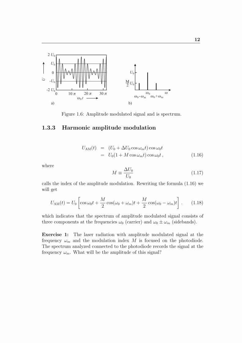
Figure 1.6: Amplitude modulated signal and is spectrum.

1.3.3 Harmonic amplitude modulation

UAM(t) = (U0 +∆U0 cosωmt) cosω0t

= U0(1 +M cosωmt) cosω0t , (1.16)

where

M ≡ ∆U0

U0

(1.17)

calls the index of the amplitude modulation. Rewriting the formula (1.16) wewill get

UAM(t) = U0

[cosω0t+

M

2cos(ω0 + ωm)t+

M

2cos(ω0 − ωm)t

]. (1.18)

which indicates that the spectrum of amplitude modulated signal consists ofthree components at the frequencies ω0 (carrier) and ω0 ± ωm (sidebands).

Exercise 1: The laser radiation with amplitude modulated signal at thefrequency ωm and the modulation index M is focused on the photodiode.The spectrum analyzed connected to the photodiode records the signal at thefrequency ωm. What will be the amplitude of this signal?

13

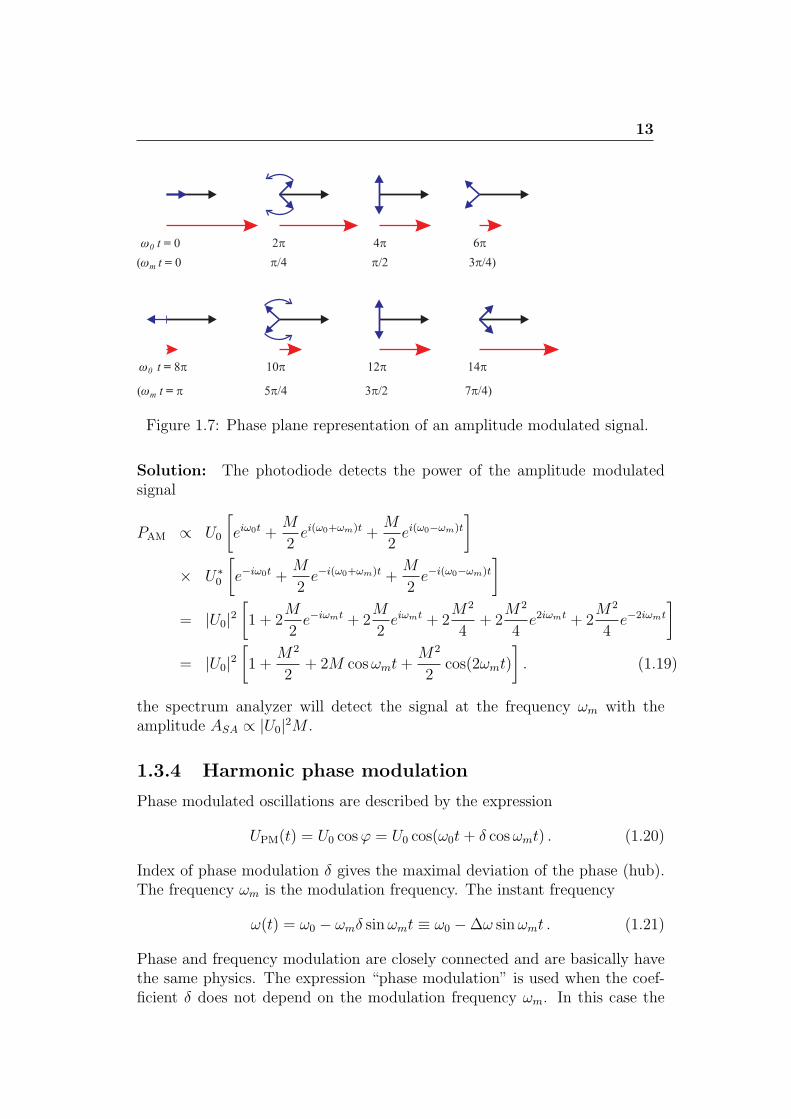
Figure 1.7: Phase plane representation of an amplitude modulated signal.

Solution: The photodiode detects the power of the amplitude modulatedsignal

PAM ∝ U0

[eiω0t +

M

2ei(ω0+ωm)t +

M

2ei(ω0−ωm)t

]× U∗

0

[e−iω0t +

M

2e−i(ω0+ωm)t +

M

2e−i(ω0−ωm)t

]= |U0|2

[1 + 2

M

2e−iωmt + 2

M

2eiωmt + 2

M2

4+ 2

M2

4e2iωmt + 2

M2

4e−2iωmt

]= |U0|2

[1 +

M2

2+ 2M cosωmt+

M2

2cos(2ωmt)

]. (1.19)

the spectrum analyzer will detect the signal at the frequency ωm with theamplitude ASA ∝ |U0|2M .

1.3.4 Harmonic phase modulation

Phase modulated oscillations are described by the expression

UPM(t) = U0 cosφ = U0 cos(ω0t+ δ cosωmt) . (1.20)

Index of phase modulation δ gives the maximal deviation of the phase (hub).The frequency ωm is the modulation frequency. The instant frequency

ω(t) = ω0 − ωmδ sinωmt ≡ ω0 −∆ω sinωmt . (1.21)

Phase and frequency modulation are closely connected and are basically havethe same physics. The expression “phase modulation” is used when the coef-ficient δ does not depend on the modulation frequency ωm. In this case the

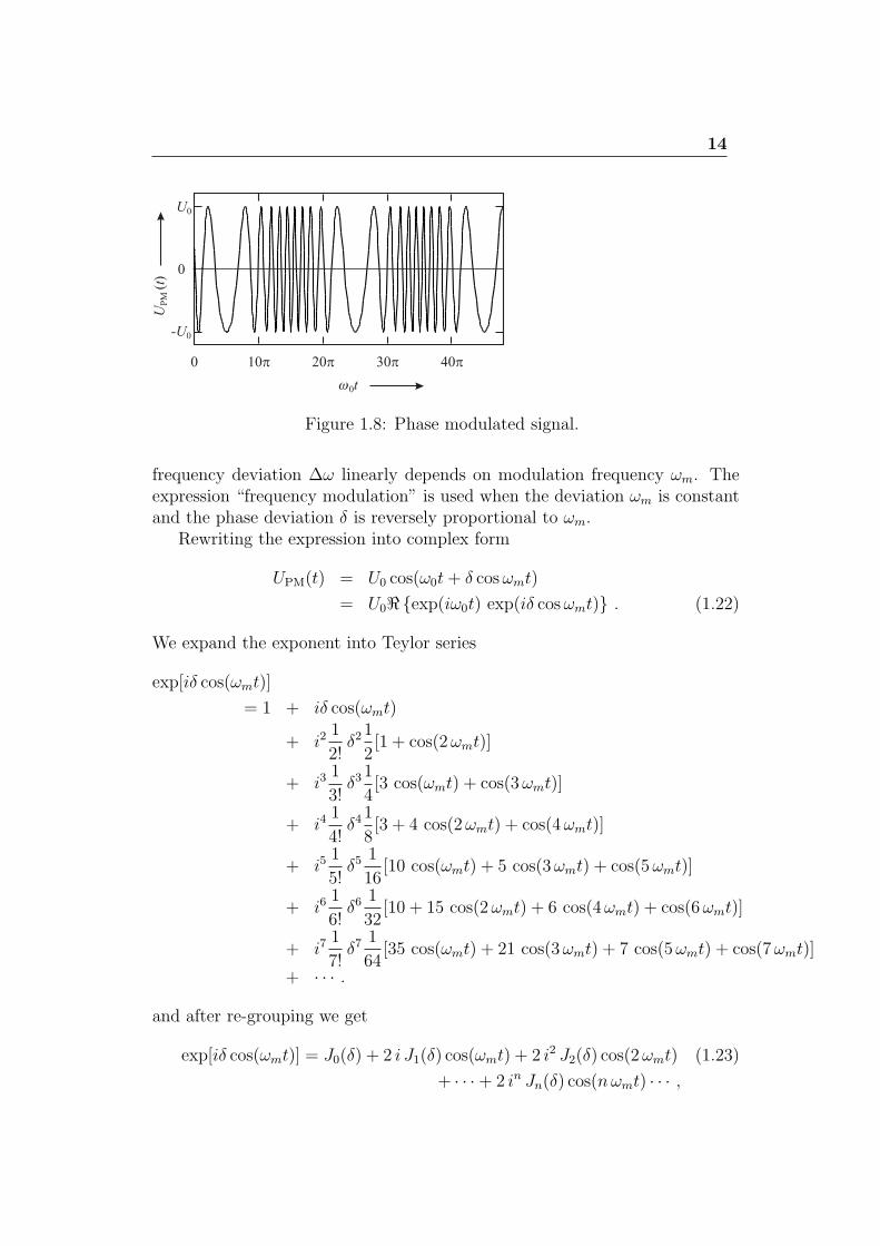
14

Figure 1.8: Phase modulated signal.

frequency deviation ∆ω linearly depends on modulation frequency ωm. Theexpression “frequency modulation” is used when the deviation ωm is constantand the phase deviation δ is reversely proportional to ωm.

Rewriting the expression into complex form

UPM(t) = U0 cos(ω0t+ δ cosωmt)

= U0ℜexp(iω0t) exp(iδ cosωmt) . (1.22)

We expand the exponent into Teylor series

exp[iδ cos(ωmt)]

= 1 + iδ cos(ωmt)

+ i21

2!δ21

2[1 + cos(2ωmt)]

+ i31

3!δ31

4[3 cos(ωmt) + cos(3ωmt)]

+ i41

4!δ41

8[3 + 4 cos(2ωmt) + cos(4ωmt)]

+ i51

5!δ5

1

16[10 cos(ωmt) + 5 cos(3ωmt) + cos(5ωmt)]

+ i61

6!δ6

1

32[10 + 15 cos(2ωmt) + 6 cos(4ωmt) + cos(6ωmt)]

+ i71

7!δ7

1

64[35 cos(ωmt) + 21 cos(3ωmt) + 7 cos(5ωmt) + cos(7ωmt)]

+ · · · .

and after re-grouping we get

exp[iδ cos(ωmt)] = J0(δ) + 2 i J1(δ) cos(ωmt) + 2 i2 J2(δ) cos(2ωmt) (1.23)

+ · · ·+ 2 in Jn(δ) cos(nωmt) · · · ,

15

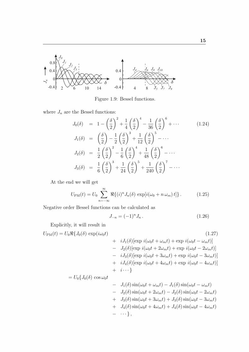
Figure 1.9: Bessel functions.

where Jn are the Bessel functions:

J0(δ) = 1−(δ

2

)2

+1

4

(δ

2

)4

− 1

36

(δ

2

)6

+ · · · (1.24)

J1(δ) =

(δ

2

)− 1

2

(δ

2

)3

+1

12

(δ

2

)5

− · · ·

J2(δ) =1

2

(δ

2

)2

− 1

6

(δ

2

)4

+1

48

(δ

2

)6

− · · ·

J3(δ) =1

6

(δ

2

)3

+1

24

(δ

2

)5

+1

240

(δ

2

)7

− · · ·

At the end we will get

UPM(t) = U0

∞∑n=−∞

ℜ(i)nJn(δ) exp[i(ω0 + nωm) t] . (1.25)

Negative order Bessel functions can be calculated as

J−n = (−1)nJn . (1.26)

Explicitly, it will result in

UPM(t) = U0ℜJ0(δ) exp(iω0t) (1.27)

+ iJ1(δ)[exp i(ω0t+ ωmt) + exp i(ω0t− ωmt)]

− J2(δ)[exp i(ω0t+ 2ωmt) + exp i(ω0t− 2ωmt)]

− iJ3(δ)[exp i(ω0t+ 3ωmt) + exp i(ω0t− 3ωmt)]

+ iJ4(δ)[exp i(ω0t+ 4ωmt) + exp i(ω0t− 4ωmt)]

+ i · · · = U0J0(δ) cosω0t

− J1(δ) sin(ω0t+ ωmt)− J1(δ) sin(ω0t− ωmt)

− J2(δ) sin(ω0t+ 2ωmt)− J2(δ) sin(ω0t− 2ωmt)

+ J3(δ) sin(ω0t+ 3ωmt) + J3(δ) sin(ω0t− 3ωmt)

+ J4(δ) sin(ω0t+ 4ωmt) + J4(δ) sin(ω0t− 4ωmt)

− · · · ,

16

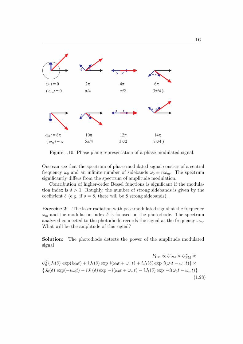
Figure 1.10: Phase plane representation of a phase modulated signal.

One can see that the spectrum of phase modulated signal consists of a centralfrequency ω0 and an infinite number of sidebands ω0 ± nωm. The spectrumsignificantly differs from the spectrum of amplitude modulation.

Contribution of higher-order Bessel functions is significant if the modula-tion index is δ > 1. Roughly, the number of strong sidebands is given by thecoefficient δ (e.g. if δ = 8, there will be 8 strong sidebands).

Exercise 2: The laser radiation with pase modulated signal at the frequencyωm and the modulation index δ is focused on the photodiode. The spectrumanalyzed connected to the photodiode records the signal at the frequency ωm.What will be the amplitude of this signal?

Solution: The photodiode detects the power of the amplitude modulatedsignal

PPM ∝ UPM × U∗PM ≈

U20J0(δ) exp(iω0t) + iJ1(δ) exp i(ω0t+ ωmt) + iJ1(δ) exp i(ω0t− ωmt) ×

J0(δ) exp(−iω0t)− iJ1(δ) exp −i(ω0t+ ωmt)− iJ1(δ) exp −i(ω0t− ωmt)(1.28)

17

Focussing only on the terms at the modulation frequency +ωm we will get

ASA(ωm) ∝ −iJ0J1 exp(iω0t) exp(−iω0t) exp(iωmt) +

iJ0J1 exp(−iω0t) exp(iω0t) exp(iωmt) =

0

(1.29)

The spectrum analyzer will detect the signal at the frequency ωm withZERO amplitude. It results from the fact that the sidebands have differentphases. Compare to result of the Exercise 1.

Lecture 2: Amplitude and phasefluctuations

Mathematical description of stochastic processes, distribution function, meanvalue, dispersion. Allan deviation. Correlated fluctuations. Autocorrelationfunction. Spectral density. Wiener-Khinchin theorem. Stochastic processes inphysical systems. From spectral representation of fluctuations to time repre-sentation. Spectral density and Allan deviation of different fluctuation types.

2.1 Mathematical description of stochastic pro-

cesses, distribution function, mean value,

dispersion.

Output frequency even of the best frequency synthesizers is not constant, butfluctuates in time. For example, harmonic amplitude and phase modulationchange the output frequency. In real life perturbations have a stochastical na-ture and should be described in a corresponding framework. The fluctuationscan be introduced mathematically as following

U(t) = [U0 +∆U(t)] cos(2πν0t+ ϕ(t)) . (2.1)

where ∆U(t) is the stochastic fluctuations of amplitude and ϕ(t) stands for thephase fluctuations. For comparison of different sources oscillating at differentfrequencies let us introduce normalized phase

x(t) ≡ ϕ(t)

2πν0, (2.2)

and frequency fluctuations

y(t) ≡ ∆ν(t)

ν0=dx(t)

dt. (2.3)

Let us then consider some value y(t) fluctuating in time. In physical ex-periment we always use discretisation, reading the value by some device (the

19

latter expression is usual for frequency measurement devices)

yi =1

τ

∫ ti+τ

ti

y(t)dt . (2.4)

so we get a set of randomly distributed numbers with some distribution func-tion which will depend on the stochastic process nature.

We can calculate the average value

y =1

N

N∑i=1

yi (2.5)

and the dispersion

S2y =

1

N − 1

N∑i=1

(yi − y)2 =1

N − 1

N∑i=1

y2i −1

N − 1

(N∑i=1

yi

)2 . (2.6)

The width of the distribution will be given by a dispersion

sy =sy√N. (2.7)

If the process is stationary (both y and sy do not depend on time) than accord-ing to the central theorem, the distribution will approach Gaussian distributionif T → ∞.

p(y) =1

σ√2π

exp

(−(y − y)2

2σ2

), (2.8)

The stochastic process is characterized by the expectation value (mean value)

⟨y⟩ =∫ ∞

−∞yp(y) dy (2.9)

and the dispersion

σ2 =

∫ ∞

−∞(y − ⟨y⟩)2p(y) dy . (2.10)

The latter can be rewritten as

σ2 = ⟨(y − ⟨y⟩)2⟩ = ⟨y2⟩ − ⟨y2⟩ . (2.11)

In real experiment we can only evaluate expectation value and the dispersion.Expectation and the dispersion can be also evaluated from the measurementresults on the ensemble of devices. Typically it is impossible. But, for astationary process the result should not depend on whether one picks up valuesfrom an ensemble of the the devices of from a time realization of one of one of

20

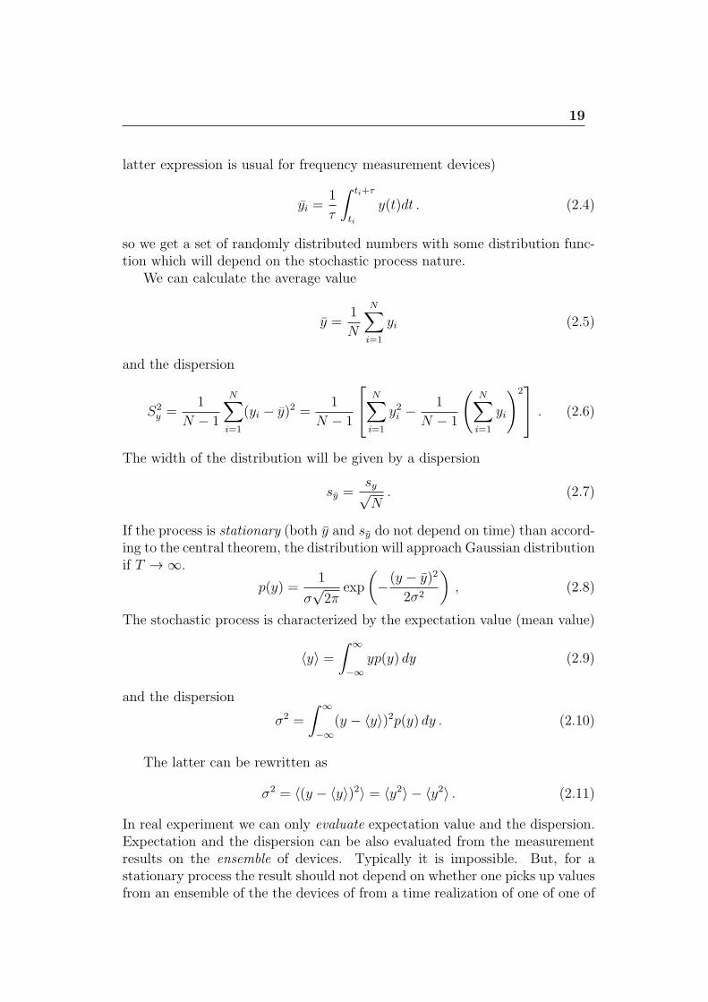
Figure 2.1: Illustration to deriving of the dispersion. a) Recorded signal. b)Digitized signal. c) Averaged signal over intervals τ .d) Histogram. e) itsapproximation by Gaussian function.

them. These processes are called ergodic processes. Very often for modellingsome processes one uses the assumptions about stationarity and ergodicityimplicitly, but one has to be quite accurate doing it. For example, if noisegrows continuously in time than the process is not stationary any more.

Another important issue is the possible existence of correlations. If fluctu-ating values are not completely independent, it will result in correlations. Iftwo sets of values, e.g. xi and yi are correlated, the plot xi(yi) will not be sym-metrical. If it is one realization of parameters, the correlation may appear asthe fact that the different subsets will have different, statistically inconsistentmean values and dispersion.

2.2 Allan deviation.

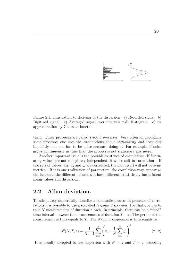
To adequately numerically describe a stochastic process in presence of corre-lations it is possible to use a so-called N-point dispersion. For that one has totake N measurements of duration τ each. In principle, there can be a “dead”time interval between the measurements of duration T − τ . The period of themeasurement is thus equals to T . The N -point dispersion is thus equals to

σ2(N, T, τ) =1

N − 1

N∑i=1

(yi −

1

N

N∑j=1

yj

)2

. (2.12)

It is usually accepted to use dispersion with N = 2 and T = τ according

21

Figure 2.2: Measurement sequence for Allan deviation.

to suggestion of Dave Allan. It is so-called Allan deviation which is usuallydenoted as σ2

y(2, τ) or σ2y(τ)

σ2y(τ) =

⟨2∑

i=1

(yi −

1

2

2∑j=1

yj

)2⟩=

1

2⟨(y2 − y1)

2⟩ . (2.13)

It is based on the measurement of the differences of the neighboring measure-ments and not on the deviation from the mean value as in the case of theregular dispersion. The square root of the Allan dispersion is called as Allandeviation.

The Allan deviation for the phase is given as

σ2y(τ) =

1

2τ 2⟨(xi+2 − 2xi+1 + xi)

2⟩. (2.14)

since

yi =xi+1 − xi

τ. (2.15)

Practical definition of Allan dispersion

To measure the frequency of some oscillator “1” and, correspondingly, its Allandeviation one has to compare the frequency of this oscillator with some otherone (“2”), preferably, much more stable. In general, we can measure only thefrequency ratio, taking one of the signals as an etalon one.

To measure the Allan dispersion one has to do the following

• measure the frequency of of the oscillator “1” compared to “2”

• the counter should operate in so-called Π-mode without a dead time(τ = T )

• calculate differences of the neighboring readings νi and νi+1, square itand divide by 2

It takes a lot of time to measure the Allan deviation for a set of differenttime intervals τ . Typically, for saving time the measurement is done by thefollowing procedure:

22

• one measures the set of νi for the minimal time interval τmin whichcounter can provide (without a dead time!)

• calculation of the Allan deviation for the minimal time σy(τmin) is givenby a standard procedure described above

• one can calculate Allan deviation for nτmin using the same dataset, n isthe integer number. Corresponding frequency is obtained by averagingcorresponding n neighboring frequency readings. E.g. for n = 3. τ =3τmin, y1,τ = (y1,τmin

+ y2,τmin+ y3,τmin

)/3, y2,τ = (y2,τmin+ y3,τmin

+y4,τmin

)/3, y3,τ = . . ..

If one of the oscillators is much more stable than the other one, than themeasurement will give the stability of studied oscillator “1”. Another casewhich is easy to interpret is when one compares two identical oscillators. Inthat case the Allan dispersion of one of the oscillators will be given as

σ2y,tot(τ) = σ2

y,1(τ) + σ2y,2(τ) and

σy,1(τ) = σy,2(τ) =1√2σy,tot(τ). (2.16)

Allan deviation is a very useful measure of an oscillator stability which allowsto characterize the stability depending on the observation time. For example,frequency-stabilized lasers possess a short time stability of σy ≤ 5 × 10−16 onthe time intervals of 1 - 100 s. For longer time intervals the Allan deviationgrows due to frequency drifts. For time intervals 1000 - 10000 s hydrogen maseroffers better stability and lower Allan deviation of σy ≤ 1 × 10−15. One canalso distinguish different dependencies for Allan deviation σy(τ) which dependon the dominating noise type. We will discuss it laser.

As an example let us first consider some deterministic frequency changes.

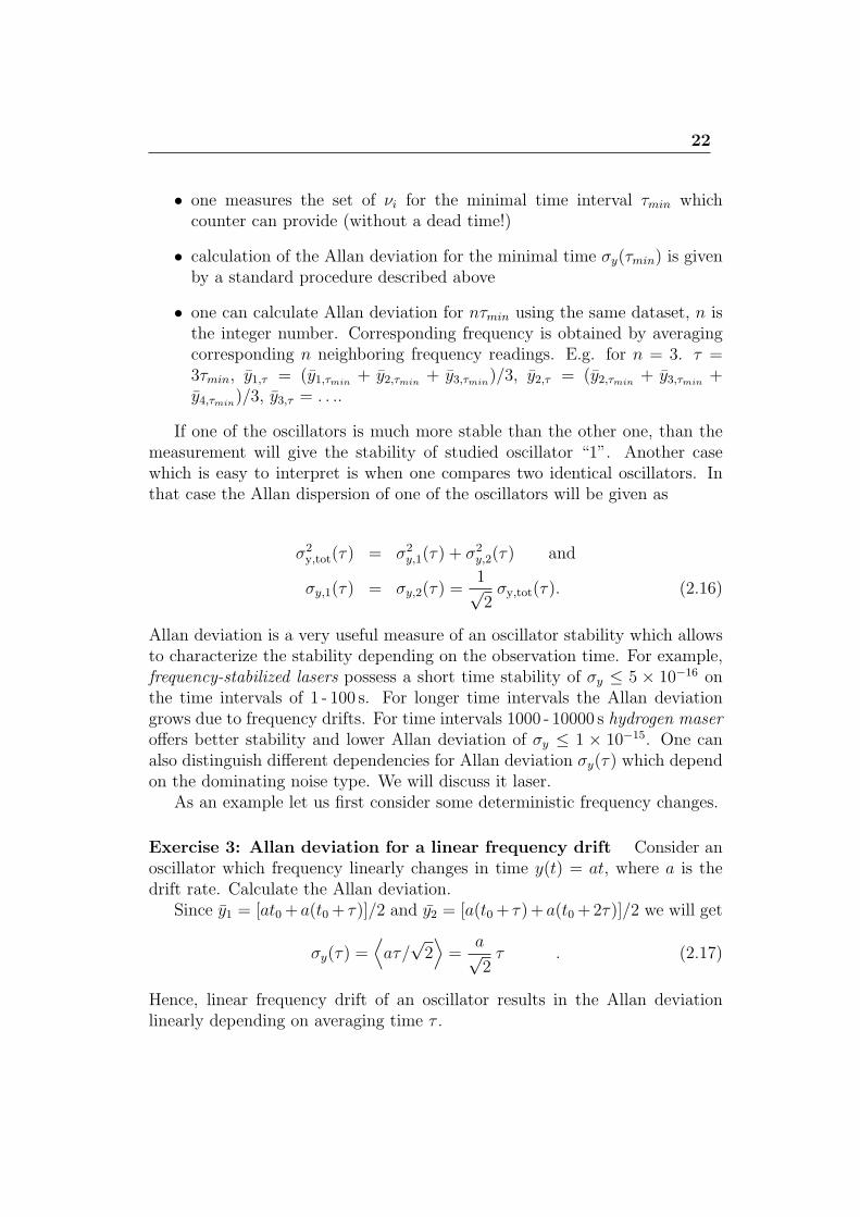
Exercise 3: Allan deviation for a linear frequency drift Consider anoscillator which frequency linearly changes in time y(t) = at, where a is thedrift rate. Calculate the Allan deviation.

Since y1 = [at0+a(t0+ τ)]/2 and y2 = [a(t0+ τ)+a(t0+2τ)]/2 we will get

σy(τ) =⟨aτ/

√2⟩=

a√2τ . (2.17)

Hence, linear frequency drift of an oscillator results in the Allan deviationlinearly depending on averaging time τ .

23

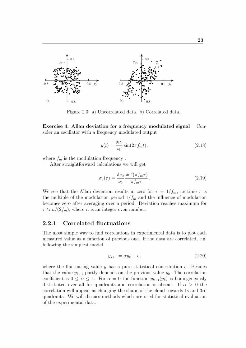
Figure 2.3: a) Uncorrelated data. b) Correlated data.

Exercise 4: Allan deviation for a frequency modulated signal Con-sider an oscillator with a frequency modulated output

y(t) =δν0ν0

sin(2πfmt) , (2.18)

where fm is the modulation frequency .After straightforward calculations we will get

σy(τ) =δν0ν0

sin2(πfmτ)

πfmτ. (2.19)

We see that the Allan deviation results in zero for τ = 1/fm, i.e time τ isthe multiple of the modulation period 1/fm and the influence of modulationbecomes zero after averaging over a period. Deviation reaches maximum forτ ≈ n/(2fm), where n is an integer even number.

2.2.1 Correlated fluctuations

The most simple way to find correlations in experimental data is to plot eachmeasured value as a function of previous one. If the data are correlated, e.g.following the simplest model

yk+1 = αyk + ϵ , (2.20)

where the fluctuating value y has a pure statistical contribution ϵ. Besidesthat the value yk+1 partly depends on the previous value yk. The correlationcoefficient is 0 ≤ α ≤ 1. For α = 0 the function yk+1(yk) is homogeneouslydistributed over all for quadrants and correlation is absent. If α > 0 thecorrelation will appear as changing the shape of the cloud towards 1s and 3rdquadrants. We will discuss methods which are used for statistical evaluationof the experimental data.

24

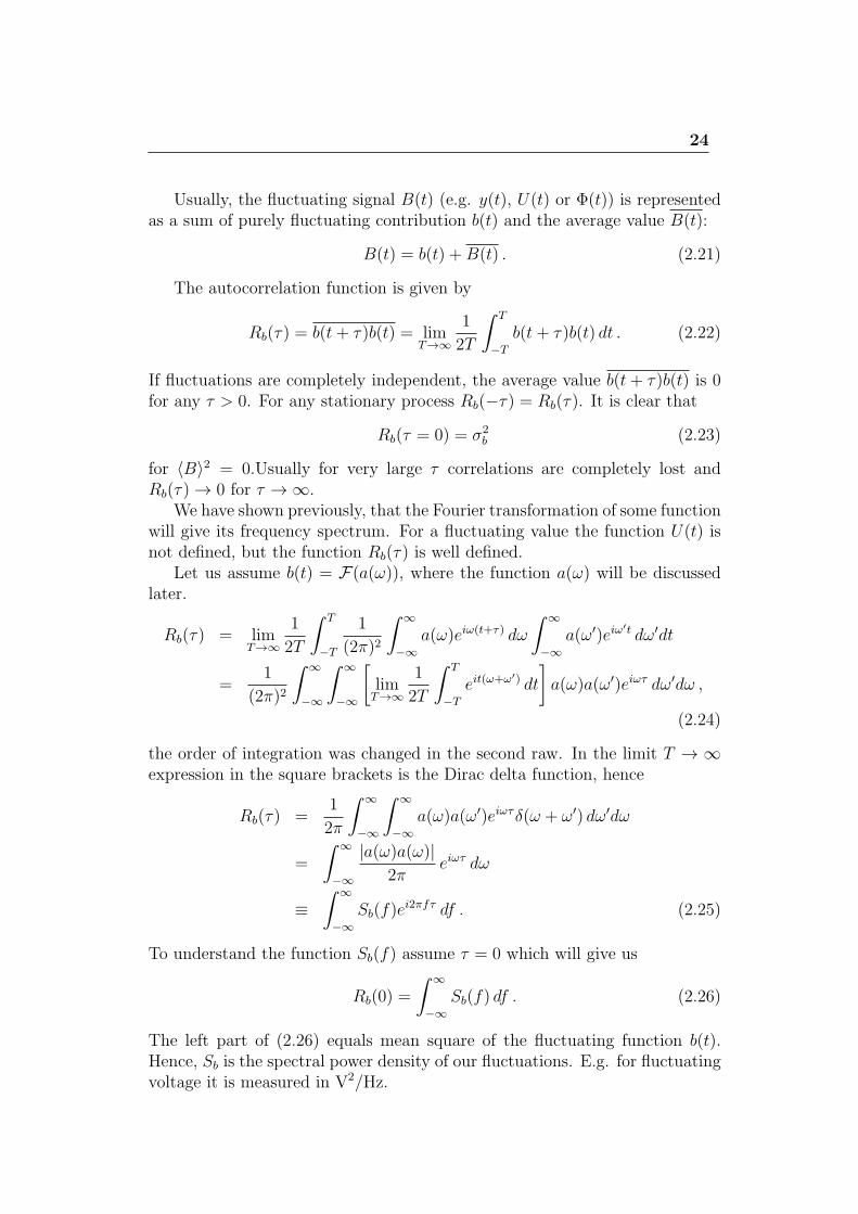
Usually, the fluctuating signal B(t) (e.g. y(t), U(t) or Φ(t)) is representedas a sum of purely fluctuating contribution b(t) and the average value B(t):

B(t) = b(t) +B(t) . (2.21)

The autocorrelation function is given by

Rb(τ) = b(t+ τ)b(t) = limT→∞

1

2T

∫ T

−T

b(t+ τ)b(t) dt . (2.22)

If fluctuations are completely independent, the average value b(t+ τ)b(t) is 0for any τ > 0. For any stationary process Rb(−τ) = Rb(τ). It is clear that

Rb(τ = 0) = σ2b (2.23)

for ⟨B⟩2 = 0.Usually for very large τ correlations are completely lost andRb(τ) → 0 for τ → ∞.

We have shown previously, that the Fourier transformation of some functionwill give its frequency spectrum. For a fluctuating value the function U(t) isnot defined, but the function Rb(τ) is well defined.

Let us assume b(t) = F(a(ω)), where the function a(ω) will be discussedlater.

Rb(τ) = limT→∞

1

2T

∫ T

−T

1

(2π)2

∫ ∞

−∞a(ω)eiω(t+τ) dω

∫ ∞

−∞a(ω′)eiω

′t dω′dt

=1

(2π)2

∫ ∞

−∞

∫ ∞

−∞

[limT→∞

1

2T

∫ T

−T

eit(ω+ω′) dt

]a(ω)a(ω′)eiωτ dω′dω ,

(2.24)

the order of integration was changed in the second raw. In the limit T → ∞expression in the square brackets is the Dirac delta function, hence

Rb(τ) =1

2π

∫ ∞

−∞

∫ ∞

−∞a(ω)a(ω′)eiωτδ(ω + ω′) dω′dω

=

∫ ∞

−∞

|a(ω)a(ω)|2π

eiωτ dω

≡∫ ∞

−∞Sb(f)e

i2πfτ df . (2.25)

To understand the function Sb(f) assume τ = 0 which will give us

Rb(0) =

∫ ∞

−∞Sb(f) df . (2.26)

The left part of (2.26) equals mean square of the fluctuating function b(t).Hence, Sb is the spectral power density of our fluctuations. E.g. for fluctuatingvoltage it is measured in V2/Hz.

25

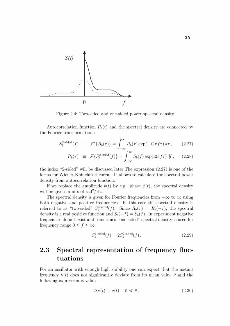
Figure 2.4: Two-sided and one-sided power spectral density.

Autocorrelation function Rb(t) and the spectral density are connected bythe Fourier transformation :

S2-sidedb (f) ≡ F∗Rb(τ) =

∫ ∞

−∞Rb(τ) exp(−i2πfτ) dτ , (2.27)

Rb(τ) ≡ FS2-sidedb (f) =

∫ ∞

−∞Sb(f) exp(i2πfτ) df , (2.28)

the index “2-sided” will be discussed later.The expression (2.27) is one of theforms for Wiener-Khinchin theorem. It allows to calculate the spectral powerdensity from autocorrelation function.

If we replace the amplitude b(t) by e.g. phase ϕ(t), the spectral densitywill be given in nits of rad2/Hz.

The spectral density is given for Fourier frequencies from −∞ to ∞ usingboth negative and positive frequencies. In this case the spectral density isreferred to as “two-sided” S2-sided

b (f). Since Rb(τ) = Rb(−τ), the spectraldensity is a real positive function and Sb(−f) = Sb(f). In experiment negativefrequencies do not exist and sometimes “one-sided” spectral density is used forfrequency range 0 ≤ f ≤ ∞:

S1-sidedb (f) = 2S2-sided

b (f) . (2.29)

2.3 Spectral representation of frequency fluc-

tuations

For an oscillator with enough high stability one can expect that the instantfrequency ν(t) does not significantly deviate from its mean value ν and thefollowing expression is valid:

∆ν(t) ≡ ν(t)− ν ≪ ν . (2.30)

26

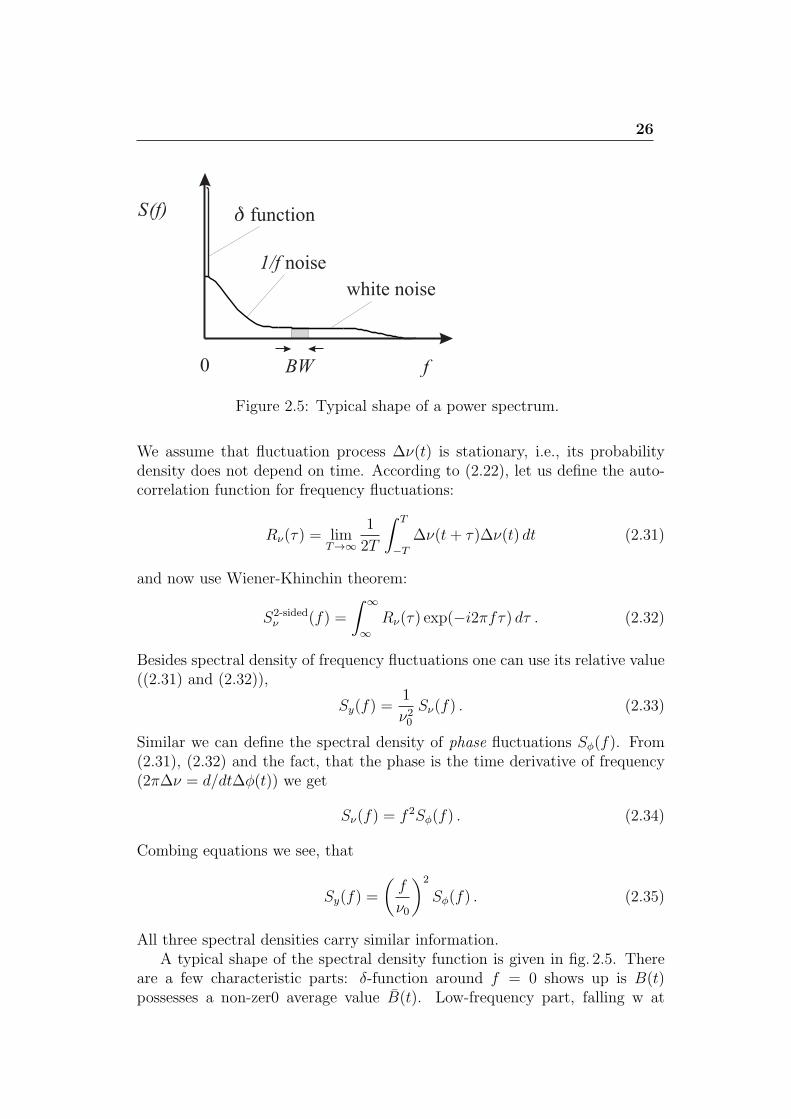
Figure 2.5: Typical shape of a power spectrum.

We assume that fluctuation process ∆ν(t) is stationary, i.e., its probabilitydensity does not depend on time. According to (2.22), let us define the auto-correlation function for frequency fluctuations:

Rν(τ) = limT→∞

1

2T

∫ T

−T

∆ν(t+ τ)∆ν(t) dt (2.31)

and now use Wiener-Khinchin theorem:

S2-sidedν (f) =

∫ ∞

∞Rν(τ) exp(−i2πfτ) dτ . (2.32)

Besides spectral density of frequency fluctuations one can use its relative value((2.31) and (2.32)),

Sy(f) =1

ν20Sν(f) . (2.33)

Similar we can define the spectral density of phase fluctuations Sϕ(f). From(2.31), (2.32) and the fact, that the phase is the time derivative of frequency(2π∆ν = d/dt∆ϕ(t)) we get

Sν(f) = f2Sϕ(f) . (2.34)

Combing equations we see, that

Sy(f) =

(f

ν0

)2

Sϕ(f) . (2.35)

All three spectral densities carry similar information.A typical shape of the spectral density function is given in fig. 2.5. There

are a few characteristic parts: δ-function around f = 0 shows up is B(t)possesses a non-zer0 average value B(t). Low-frequency part, falling w at

27

higher frequencies is referred to as 1/f noise. A flat, frequency-independentpart corresponds to white noise. Full power in the fluctuations is given by:∫ ∞

0

S1-sidedν (f) df =

∫ ∞

−∞S2-sidedν (f) df = ⟨[∆ν(t)]2⟩ = σ2

ν . (2.36)

Here we used expressions (2.23) and (2.26). Since power should be finite, athigher frequencies the spectral density should vanish (fig 2.5).

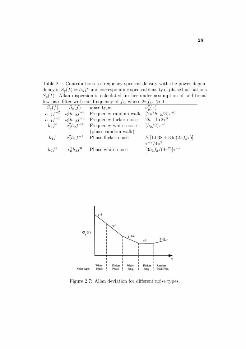
Measurements of different stable frequency oscillators (from quartz oscilla-tors to atomic clocks) show, that the fluctuations of noise spectral density maybe well approximated by combination of 5 independent noise processes withspectral density functions represented by power series of f (see table 2.1):

Sy(f) =2∑

α=−2

hαfα . (2.37)

These noise components correspondingly have typical shape in time represen-tation as shown in fig. 2.6.

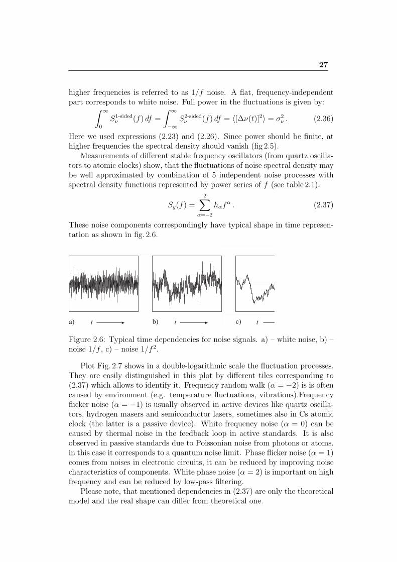
Figure 2.6: Typical time dependencies for noise signals. a) – white noise, b) –noise 1/f , c) – noise 1/f2.

Plot Fig. 2.7 shows in a double-logarithmic scale the fluctuation processes.They are easily distinguished in this plot by different tiles corresponding to(2.37) which allows to identify it. Frequency random walk (α = −2) is is oftencaused by environment (e.g. temperature fluctuations, vibrations).Frequencyflicker noise (α = −1) is usually observed in active devices like quartz oscilla-tors, hydrogen masers and semiconductor lasers, sometimes also in Cs atomicclock (the latter is a passive device). White frequency noise (α = 0) can becaused by thermal noise in the feedback loop in active standards. It is alsoobserved in passive standards due to Poissonian noise from photons or atoms.in this case it corresponds to a quantum noise limit. Phase flicker noise (α = 1)comes from noises in electronic circuits, it can be reduced by improving noisecharacteristics of components. White phase noise (α = 2) is important on highfrequency and can be reduced by low-pass filtering.

Please note, that mentioned dependencies in (2.37) are only the theoreticalmodel and the real shape can differ from theoretical one.

28

Table 2.1: Contributions to frequency spectral density with the power depen-dency of Sy(f) = hαf

α and corresponding spectral density of phase fluctuationsSϕ(f). Allan dispersion is calculated further under assumption of additionallow-pass filter with cut frequency of fh, where 2πfhτ ≫ 1.Sy(f) Sϕ(f) noise type σ2

y(τ)

h−2f−2 ν20h−2f

−4 Frequency random walk (2π2h−2/3)τ+1

h−1f−1 ν20h−2f

−3 Frequency flicker noise 2h−1 ln 2τ0

h0f0 ν20h0f

−2 Frequency white noise (h0/2)τ−1

(phase random walk)h1f ν20h1f

−1 Phase flicker noise h1[1.038 + 3 ln(2πfhτ)]·τ−2/4π2

h2f2 ν20h2f

0 Phase white noise [3h2fh/(4π2)]τ−2

Figure 2.7: Allan deviation for different noise types.

29

2.4 From spectral representation of fluctua-

tions to time representation

Up to now we described the instability of oscillators either as Fourier trans-formation (spectral density) or as Allan deviation (time representation). Weshow here how to calculate Allan deviation from a known spectral density.

Allan dispersion given by (2.13) can be written as

σ2y(τ) =

1

2⟨(y2 − y1)

2⟩ = 1

2

⟨(1

τ

∫ tk+2

tk+1

y(t′) dt′ − 1

τ

∫ tk+1

tk

y(t′) dt′

)2⟩,

(2.38)where tk+i − tk = iτ for integer i. In the expression (2.38) each counted valueis equal to half of difference of two squared values of y(t) for two next intervalsof length τ and Allan dispersion is obtained as a mean expected value. To getmore information one can substitute a discreet values of y(t′) by an integralrepresentation :

σ2y(τ) =

⟨1

2

(1

τ

∫ t+τ

t

y(t′) dt′ − 1

τ

∫ t

t−τ

y(t′) dt′)2⟩. (2.39)

Expression (2.39) can be rewritten as following:

σ2y(τ) =

⟨(∫ ∞

−∞y(t′)hτ (t− t′) dt′

)2⟩, (2.40)

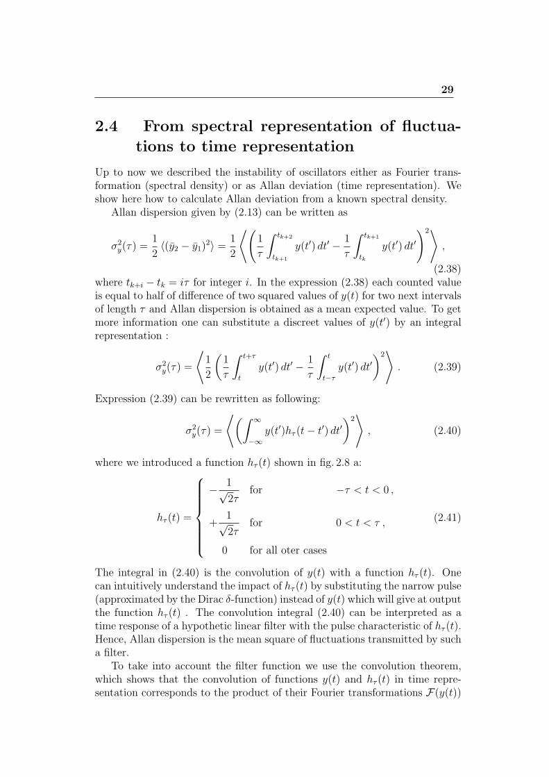
where we introduced a function hτ (t) shown in fig. 2.8 a:

hτ (t) =

− 1√2τ

for −τ < t < 0 ,

+1√2τ

for 0 < t < τ ,

0 for all oter cases

(2.41)

The integral in (2.40) is the convolution of y(t) with a function hτ (t). Onecan intuitively understand the impact of hτ (t) by substituting the narrow pulse(approximated by the Dirac δ-function) instead of y(t) which will give at outputthe function hτ (t) . The convolution integral (2.40) can be interpreted as atime response of a hypothetic linear filter with the pulse characteristic of hτ (t).Hence, Allan dispersion is the mean square of fluctuations transmitted by sucha filter.

To take into account the filter function we use the convolution theorem,which shows that the convolution of functions y(t) and hτ (t) in time repre-sentation corresponds to the product of their Fourier transformations F(y(t))

30

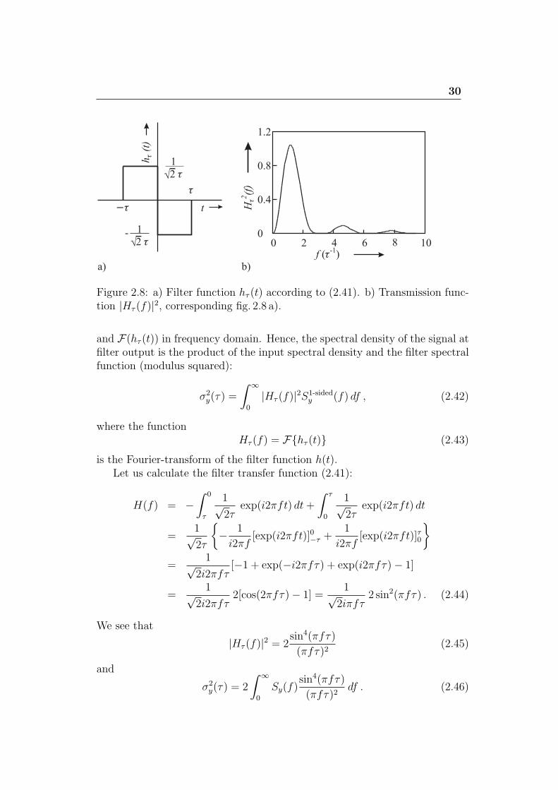
Figure 2.8: a) Filter function hτ (t) according to (2.41). b) Transmission func-tion |Hτ (f)|2, corresponding fig. 2.8 a).

and F(hτ (t)) in frequency domain. Hence, the spectral density of the signal atfilter output is the product of the input spectral density and the filter spectralfunction (modulus squared):

σ2y(τ) =

∫ ∞

0

|Hτ (f)|2S1-sidedy (f) df , (2.42)

where the functionHτ (f) = Fhτ (t) (2.43)

is the Fourier-transform of the filter function h(t).Let us calculate the filter transfer function (2.41):

H(f) = −∫ 0

τ

1√2τ

exp(i2πft) dt+

∫ τ

0

1√2τ

exp(i2πft) dt

=1√2τ

− 1

i2πf[exp(i2πft)]0−τ +

1

i2πf[exp(i2πft)]τ0

=

1√2i2πfτ

[−1 + exp(−i2πfτ) + exp(i2πfτ)− 1]

=1√

2i2πfτ2[cos(2πfτ)− 1] =

1√2iπfτ

2 sin2(πfτ) . (2.44)

We see that

|Hτ (f)|2 = 2sin4(πfτ)

(πfτ)2(2.45)

and

σ2y(τ) = 2

∫ ∞

0

Sy(f)sin4(πfτ)

(πfτ)2df . (2.46)

31

This expression allows to calculate Allan dispersion directly from (one-sided)spectral density Sy(f).

For example let us calculate Allan dispersion for phase white noise (Sy =h2f

2). Expression (2.46) gives:

σ2y(τ) = 2

∫ ∞

0

h2f2 sin

4(πfτ)

(πfτ)2df =

2h2π2τ 2

∫ ∞

0

sin4(πfτ) df . (2.47)

Integral in (2.47) does not converge at f → ∞. In the experiment it does notpose a problem since for any device the frequency bandwidth is restricted athigher frequencies. If we model this restriction by the low pass filter with thecut frequency of fh, the integral (2.47) can be calculated with the help of theexpression

∫sin4 ax dx = 3/8x− 1/(4a) sin 2ax+ 1/(32a) sin 4ax. We get:

σ2y(τ) =

2h2π2τ 2

∫ fh

0

sin4(πfτ) df =3h2fh4π2τ 2

+O(τ−3) . (2.48)

Since we can neglect the contribution O(τ−3) for fh ≫ 1/(2πτ) the Allandeviation for the phase white noise is the power function ∝ τ−2. Similarly onecan calculate σy(t) for other spectral shapes. It is summarized in the table 2.1.

Integral (2.46) diverges also for the phase flicker noise (Sy(f) = h1f). Thelow pass filtering helps to solve this problem.

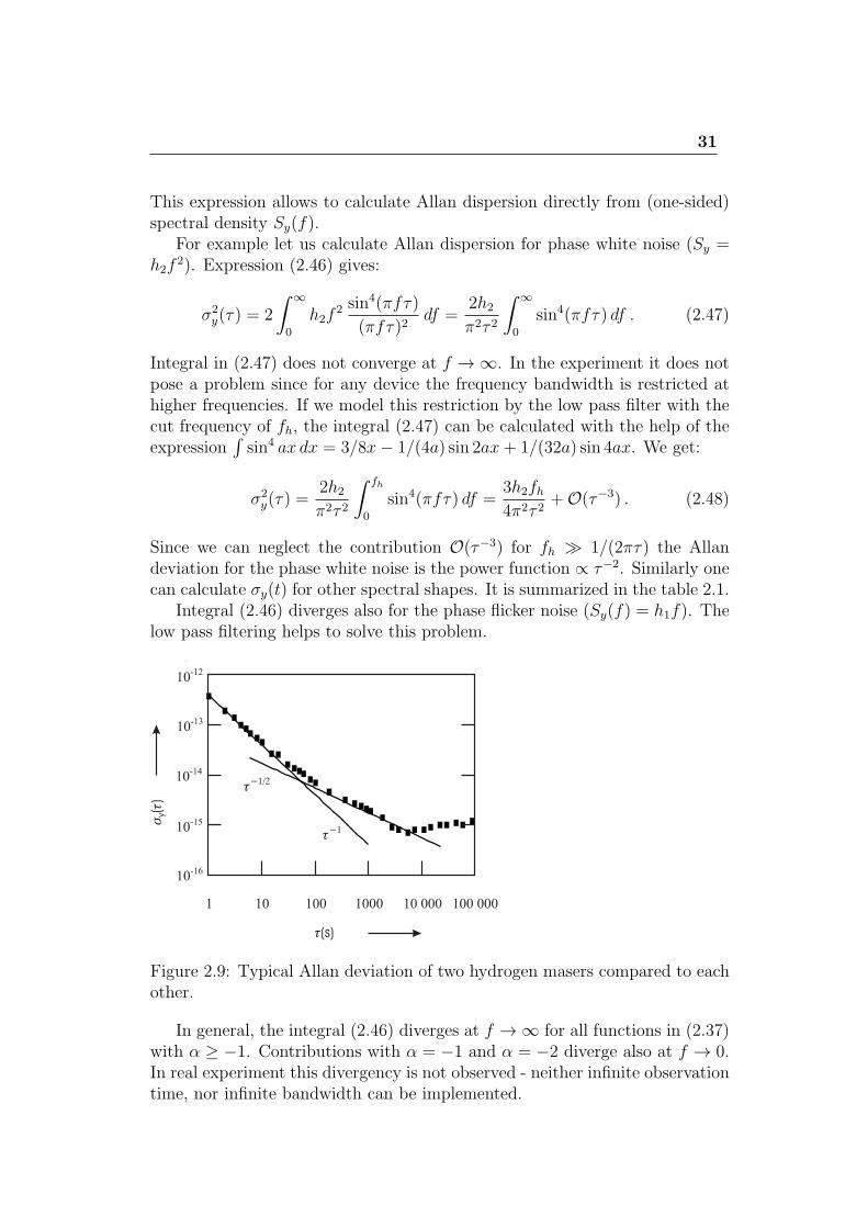
Figure 2.9: Typical Allan deviation of two hydrogen masers compared to eachother.

In general, the integral (2.46) diverges at f → ∞ for all functions in (2.37)with α ≥ −1. Contributions with α = −1 and α = −2 diverge also at f → 0.In real experiment this divergency is not observed - neither infinite observationtime, nor infinite bandwidth can be implemented.

32

Allan dispersion can be unambiguously calculated from the spectral density,but it is not reversible.

Representation with the help of Allan dispersion is widely used since it iseasily measured and calculated. At the other hand, the spectral representationcontains all information about noises. E.g. consider the Allan dispersion offor the hydrogen maser ( fig 2.9). For short integration times the phase whitenoise dominates (∝ τ−1) and also flicker phase noise (approx. prop to τ−1),for longer integration times – white frequency noise (∝ τ−1/2). Then the Allandispersion reaches its minimum called the flicker noise floor and then startsgrowing because of frequency drifts.

Lecture 3: From frequencyfluctuations to spectral lineshape

Power spectral density of a quasimonochromatic signal with a fluctuating phase.Autocorrelation function representation. Spectral line shape. Line shape in thecases of (i) shallow high-frequency fluctuations and (ii) strong low-frequencyphase fluctuations. Line width. Transformation of the line shape in non-linearprocesses like second harmonic generation.

3.1 Power spectral density of a quasimonochro-

matic signal with a fluctuating phase.

Regularly by studying spectral properties of a laser or rf oscillator one is inter-ested in a narrow spectral region around the carrier at frequency ν0. For perfectoscillator it should be a Dirac-δ function, but for a real oscillator phase fluc-tuations result in spreading of the power around some frequency band aroundν0.

The spectrum can be measured by different tools. For example, it can be anarrow-band filter which central frequency can be tuned around the carrier (inoptical region one can use a Fabri-Perot cavity). Another approach is to usea number of narrow band filters in parallel. Also it is possible to implementFast Fourier Transformation for the signal of interest.

It is still necessary to note that the concept of power spectrum with fixedshape and envelope is not applicable to all fluctuation processes. For example,the 1/f noise will not result in the well-defined line shape because of its driftingnature. The line shape will depend on the observation time in this case.

We will show here how one can calculate the line shape knowing a phasenoise spectral density Sϕ(ν). According to (2.27) and (2.28) this (two-sided)spectral density is given via Fourier transformation

SE(ν) =

∫ ∞

−∞exp(−i2πντ)RE(τ) dτ (3.1)

34

from the correlation function

RE(τ) = ⟨E(t+ τ)E∗(t)⟩ (3.2)

for the electric field E(t). We will neglect amplitude fluctuations in this case.

E(t) = E0 exp i[2πν0t+ ϕ(t)] (3.3)

Autocorrelation function looks like:

RE(τ) = E20 exp[i2πν0τ ]⟨exp i[ϕ(t+ τ)− ϕ(τ)]⟩ . (3.4)

The mean value ⟨exp i[ϕ(t+ τ)− ϕ(τ)]⟩ can be calculated via spectral phasenoise density Sϕ(f). First of all, let us assume that these fluctuations areergodic (averaging over time is equivalent to averaging over ensemble):

exp[iΦ(t, τ)] = ⟨exp[iΦ(t, τ)]⟩ =∫ ∞

−∞p(Φ) exp(iΦ) dΦ , (3.5)

whereΦ(t, τ) = ϕ(t+ τ)− ϕ(t) (3.6)

– is the phase increment over time τ . In the right part of exp. (3.5) we use aregular definition of mathematical expected value (mean) of exp[iΦ(t, τ)] forthe given probability distribution of p(Φ). For a large number of uncorrelatedevents the central limiting theorem allows to use the Gaussian probabilitydistribution

p(Φ) =1

σ√2π

exp

(− Φ2

2σ2

)(3.7)

with the regular dispersion of σ2. Since the function p(Φ) is purely real, onlythe real (cosine) part will be left in the integral (3.5). Substitution of (3.5) in(3.7), taking into account

∫∞−∞ exp(−a2x2) cos x dx =

√π/a exp(−1/4a2) will

give us:

⟨exp[iΦ(t, τ)]⟩ = exp

(−σ

2

2

). (3.8)

Using (2.11) for ⟨Φ⟩ = 0 (3.6), we get:

σ2(Φ) = ⟨Φ2⟩ = ⟨[ϕ(t+ τ)− ϕ(τ)]2⟩= ⟨[ϕ(t+ τ)]2⟩ − 2⟨[ϕ(t+ τ)ϕ(τ)]⟩+ ⟨[ϕ(τ)]2⟩ . (3.9)

From (3.2) we get:

⟨[ϕ(t+ τ)ϕ(τ)]⟩ =

∫ ∞

0

Sϕ(f) cos(2πfτ) df = Rϕ(f) , (3.10)

⟨[ϕ(t+ τ)]2⟩ = ⟨[ϕ(τ)]2⟩ =∫ ∞

0

Sϕ(f) df = Rϕ(0) . (3.11)

35

Substitution of (3.10) and (3.11) into (3.9) will give us:

σ2 = 2

∫ ∞

0

Sϕ(f)[1− cos 2πfτ ] df , (3.12)

which allows to calculate the autocorrelation function (3.4):

RE(τ) = E20 exp[i2πν0τ ] exp

(−∫ ∞

0

Sϕ(f)[1− cos 2πfτ ] df

). (3.13)

Equations (3.1) and (3.13) allow to calculate the power spectral density fromthe given spectral density of phase fluctuations Sϕ(f) (see (2.34)):

SE(ν−ν0) = E20

∫ ∞

−∞exp−[i2π(ν−ν0)τ ] exp

(−∫ ∞

0

Sϕ(f)[1− cos 2πfτ ] df

)dτ

(3.14)under condition that the integral (3.14) converges.

3.1.1 Spectrum with shallow high-frequency fluctuations

Let us consider a case of shallow high-frequency fluctuations. For simplicitylet us re-write the expression (3.14) for circular frequencies

SE(ω) = E20

∫ ∞

−∞exp−[i(ω − ω0)τ ] exp

(−∫ ∞

0

Sω(ω′)[1− cosω′τ ]

ω′2 dω′)dτ

(3.15)and define the function F (τ) as

F (τ) ≡∫ ∞

0

Sω(ω′)[1− cosω′τ ]

ω′2 dω′ . (3.16)

Let us also introduce the dispersion of frequency fluctuations according to

σ2ω = Ω

2=

∫ ∞

0

Sω(ω′)dω′ (3.17)

with Sω(ω′) being a one-sided spectral density. The fluctuation process ω(t)

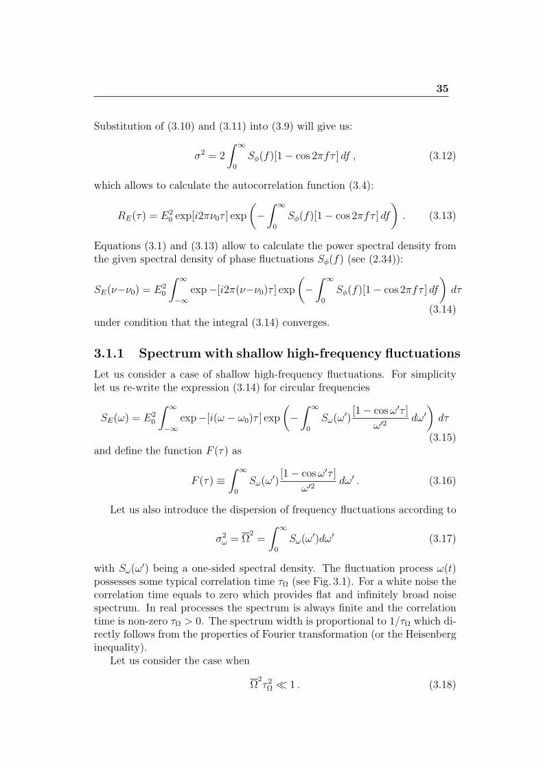
possesses some typical correlation time τΩ (see Fig. 3.1). For a white noise thecorrelation time equals to zero which provides flat and infinitely broad noisespectrum. In real processes the spectrum is always finite and the correlationtime is non-zero τΩ > 0. The spectrum width is proportional to 1/τΩ which di-rectly follows from the properties of Fourier transformation (or the Heisenberginequality).

Let us consider the case when

Ω2τ 2Ω ≪ 1 . (3.18)

36

Figure 3.1: a) Fluctuating frequency. The mean value ω0, the dispersion Ω

and the correlation time τΩ. b)Relations between Sω(0), τΩ and Ω2derived

from the typical spectrum shape.

Figure 3.2: Relation between the spectral width of shallow high-frequencyfluctuations and function [1−cosω′τ ]

ω′2 .

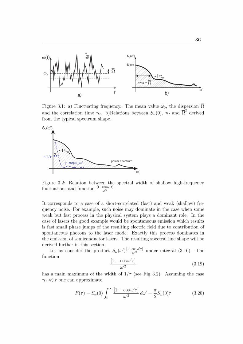
It corresponds to a case of a short-correlated (fast) and weak (shallow) fre-quency noise. For example, such noise may dominate in the case when someweak but fast process in the physical system plays a dominant role. In thecase of lasers the good example would be spontaneous emission which resultsis fast small phase jumps of the resulting electric field due to contribution ofspontaneous photons to the laser mode. Exactly this process dominates inthe emission of semiconductor lasers. The resulting spectral line shape will bederived further in this section.

Let us consider the product Sω(ω′) [1−cosω′τ ]

ω′2 under integral (3.16). Thefunction

[1− cosω′τ ]

ω′2 (3.19)

has a main maximum of the width of 1/τ (see Fig. 3.2). Assuming the caseτΩ ≪ τ one can approximate

F (τ) = Sω(0)

∫ ∞

0

[1− cosω′τ ]

ω′2 dω′ =π

2Sω(0)τ (3.20)

37

since ∫ ∞

0

1− cos bx

x2=π|b|2

. (3.21)

We obtain a diffusion process with the diffusion coefficient of

D =πSω(0)

2. (3.22)

Thus, we get for the (3.15):

SE(ω) = E20

∫ ∞

−∞exp[−Dτ ] exp−[i(ω − ω0)τ ] dτ . (3.23)

The exponent exp[−Dτ ] cuts the expression under integral at τ ≈ 1/D. Letus remember that we considered the case τΩ ≪ τ , so we get Dτ ≈ 1 andDτΩ ≪ 1. Substituting D from (3.22) we get

π

2Sω(0)τΩ ≪ 1 . (3.24)

From Fig. 3.2 one can approximate

Ω2=

∫ ∞

0

Sω(ω′)dω′ ≈ Sω(0)

τΩ, (3.25)

which gives us Sω(0) ≈ Ω2τΩ. Combining this result with (3.24) we get

π2Ω

2τ 2Ω ≪ 1 which is compatible with the initial assumption (3.18).Finally, we can easily calculate the integral (3.16)

SE(ω) = 2E20

D

D2 + (ω − ω0)2. (3.26)

This is the Lorentzian line shape.

Conclusions: for the case of shallow high-frequency noise one should expectthe Lorenzian line shape according to (3.26).

3.1.2 Spectrum with slow and deep frequency fluctua-tions

In this section we will consider different case compared to 3.1.1, namely, thecase of slow and deep fluctuations. This case corresponds mathematically to

Ω2τ 2Ω ≫ 1 (3.27)

(compare to (3.18)). This case corresponds to the situation when the oscillatorfrequency is perturbed by some slow but intense process. In case of the laser

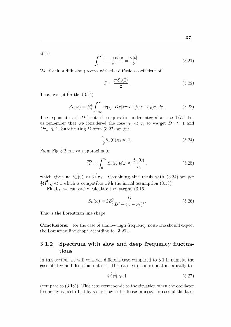
38

Figure 3.3: Relation between the spectral width of deep low-frequency fluctu-ations and a function [1−cosω′τ ]

ω′2 .

it can be acoustic noise or temperature fluctuations, or density perturbationsin gas lasers. In the intuitive picture, the oscillator frequency will randomlyfluctuate around some value and the resulting line shape will be a sum ofsome “instant prints” of the narrow lines with individually shifted frequencies.According to the Central limiting theorem one should expect Gaussian distri-bution. Let us show it mathematically. Let us assume that in this case onlytime intervals τ = 1/ω ≪ τΩ are important in our analysis. In this case

1− cos(ωτ) ≈ ω2τ 2

2(3.28)

and the integral 3.16 is given as

F (τ) = τ 2∫ ∞

0

Sω(ω′)dω′ = Ω

2τ 2 . (3.29)

Correspondingly,

SE(ω) = E20

∫ ∞

−∞exp−[i(ω − ω0)τ ] exp[−Ω

2τ 2] dτ . (3.30)

The second exponent cuts the integral at the typical time of τ 2 = 1/Ω2and,

together with assumption τ ≪ τΩ we get τ 2Ω2 ≫ 1 which is compatible with

(3.27).Taking the integral 3.30 one gets

SE(ω) =

√πE2

0

Ωe−(ω−ω0)2/4Ω

2

, (3.31)

which is the Gauusian line shape as expected from intuitive considerations.

3.1.3 Spectrum with a weak phase noise

Expression (3.14) can be transformed using (3.10) (3.11) as following:

SE(ν − ν0) = E20

∫ ∞

−∞exp[−Rϕ(0)] exp[Rϕ(τ)] exp[−i2π(ν − ν0)τ ] dτ . (3.32)

39

If phase fluctuations are weak∫∞0Sϕ(f) df ≪ 1, we can expand two first

exponents in the power series, leaving the leading order:

SE(ν − ν0) = E20

∫ ∞

−∞[1−Rϕ(0) +Rϕ(τ)] exp[−i2π(ν − ν0)τ ] dτ . (3.33)

Using definition of the Dirac-δ function and Wiener-Khinchin theorem (2.28)we get

SE(ν − ν0) = E20 [1−Rϕ(0)]δ(ν − ν0) + E2

0S2-sidedϕ (ν − ν0) . (3.34)

Power spectrum consists of the carrier frequency (δ-function) at ν = ν0 andtwo symmetrical sidebands, proportional to the spectral density of the pasenoise Sϕ for f = |ν − ν0|.

For commercial devices the useful parameter is the spectral purity L(f)which corresponds to noise level in the side band measured by spectrum ana-lyzer:

L(f) =S2-sidedϕ (ν − ν0)

1/2E20

. (3.35)

3.1.4 Spectrum with phase noise: power in the carrierand carrier collapse

Returning back to the equation (3.32)

SE(ν − ν0) = E20

∫ ∞

−∞exp[−Rϕ(0)] exp[Rϕ(τ)] exp[−i2π(ν − ν0)τ ] dτ . (3.36)

can leave the exponent exp[−Rϕ(0)] without expanding it to power series andonly expand the second one exp[Rϕ(τ)]. In this case the result (3.34) will betransformed to

SE(ν − ν0) = E20

(e−Rϕ(0)δ(ν − ν0) + e−Rϕ(0)S2-sided

ϕ (ν − ν0)). (3.37)

We see that fraction of power in the carrier (δ(ν − ν0)) is proportional to

e−Rϕ(0) = e−ϕ2rms , (3.38)

where −ϕ2rms is the dispersion of the phase fluctuations (r.m.s. phase deviation

squared). For e.g. ϕ2rms = 0 we see that the power fraction in the carrier

Pcarrier = 1 as expected for a noise-free signal. For phase fluctuations on theorder of ϕ2

rms = 1 the fraction promptly drops Pcarrier = 1/e.Let us consider a noisy signal with phase fluctuations of ϕrms. If the signal

is transformed in the second harmonic generation process, the phase deviation

40

doubles ϕ′rms = 2ϕrms which will result in the fact, that the dispersion of the

phase fluctuations will be quadrupled.

ϕ′2rms = 4ϕ2

rms . (3.39)

Accordingly, the power in the carrier will be reduced accordingly to (3.38). Ingeneral case, if the signal is converted in the nth harmonic, the power in thecarrier will change as

P ′carrier = e−ϕ′2

rms = e−n2ϕ2rms = (Pcarrier)

n2

. (3.40)

For example, if the laser light at 972 nm contains Pcarrier = 0.97 power in thecarrier, transformation in the 8th harmonic at 121 nm will result in P ′

carrier =(0.99)64 = 0.61. Even for the best oscillators, frequency multiplication willresult in the prompt growth of the phase noise contribution which can resultin a so-called carrier collapse. Intuitively one can explain such feature by thefact that the noise spectral components will multiply with the carrier in thenon-linear process of harmonic transformation which result in relative increaseof the phase noise contribution.

3.2 Measurement methods

The spectral density of frequency (or phase) fluctuations can be measured bydifferent means. Function Sν(f) can be measured with the help of spectrumanalyzer which can be modelled as a set of narrow-band filters and detectorsmeasuring power at the output of each of the filter. Other method uses digitalspectrum analyzers with built-in FFT transformation function:

∆ϕ(f) = F(∆ϕ(t)) . (3.41)

Spectral density of phase fluctuations will be given as :

Sϕ(f) =[∆ϕ(f)]2

BW, (3.42)

where the bandwidth BW should satisfy and inequality BW ≪ f .Frequency and phase fluctuations can be transformed into amplitude fluc-

tuations by using a discriminator. It can be slopes of frequency responses ofdifferent electronic filters, Fabri-Perot cavities of absorption line. If the os-cillator frequency is tuned to the slope the power at the filter output will belinearly dependent on the frequency:

V (ν − νS) = (ν − νS)kd + V (νS) , (3.43)

where kd – is the slope a the frequency nS. A detector, installed after the filterwill allow to transform frequency fluctuations in the power fluctuations (seefig. 3.4 a).

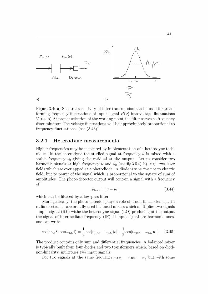
41

Figure 3.4: a) Spectral sensitivity of filter transmission can be used for trans-forming frequency fluctuations of input signal P (ν) into voltage fluctuationsV (ν). b) At proper selection of the working point the filter serves as frequencydiscriminator: The voltage fluctuations will be approximately proportional tofrequency fluctuations. (see (3.43))

3.2.1 Heterodyne measurements

Higher frequencies may be measured by implementation of a heterodyne tech-nique. In the heterodyne the studied signal at frequency ν is mixed with astable frequency ν0 giving the residual at the output. Let us consider twoharmonic signals at high frequency ν and ν0 (see fig 3.5 a), b), e.g. two laserfields which are overlapped at a photodiode. A diode is sensitive not to electricfield, but to power of the signal which is proportional to the square of sum ofamplitudes. The photo-detector output will contain a signal with a frequencyof

νbeat = |ν − ν0| (3.44)

which can be filtered by a low-pass filter.More generally, the photo-detector plays a role of a non-linear element. In

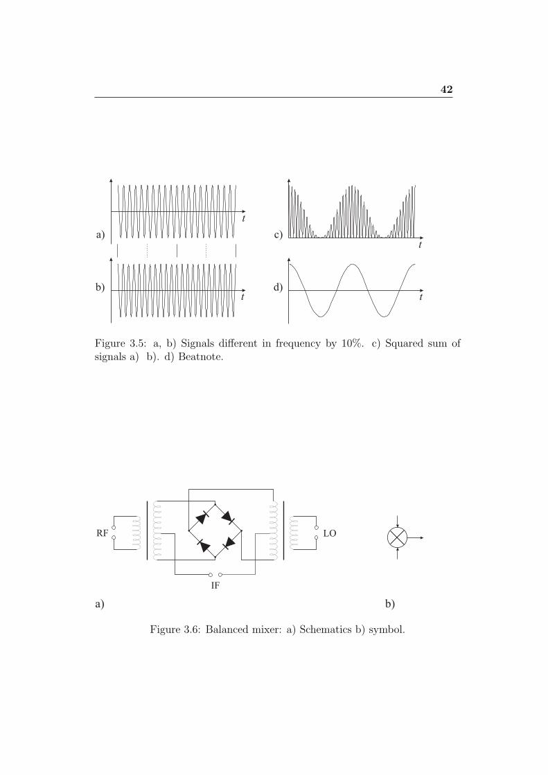
radio-electronics are broadly used balanced mixers which multiplies two signals- input signal (RF) withe the heterodyne signal (LO) producing at the outputthe signal of intermediate frequency (IF). If input signal are harmonic ones,one can write

cos(ωRFt) cos(ωLOt) =1

2cos[(ωRF + ωLO)t] +

1

2cos[(ωRF − ωLO)t] . (3.45)

The product contains only sum and differential frequencies. A balanced mixeris typically built from four diodes and two transformers which, based on diodenon-linearity, multiplies two input signals.

For two signals at the same frequency ωLO = ωRF = ω, but with some

42

Figure 3.5: a, b) Signals different in frequency by 10%. c) Squared sum ofsignals a) b). d) Beatnote.

Figure 3.6: Balanced mixer: a) Schematics b) symbol.

43

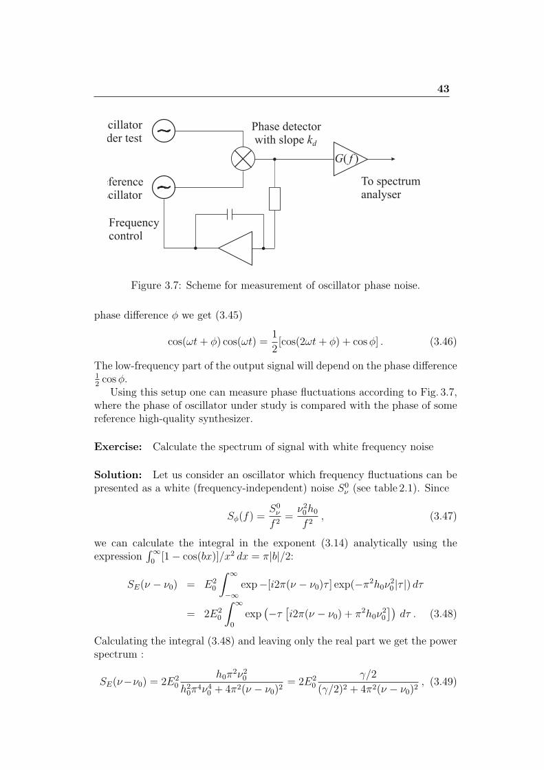
Figure 3.7: Scheme for measurement of oscillator phase noise.

phase difference ϕ we get (3.45)

cos(ωt+ ϕ) cos(ωt) =1

2[cos(2ωt+ ϕ) + cosϕ] . (3.46)

The low-frequency part of the output signal will depend on the phase difference12cosϕ.Using this setup one can measure phase fluctuations according to Fig. 3.7,

where the phase of oscillator under study is compared with the phase of somereference high-quality synthesizer.

Exercise: Calculate the spectrum of signal with white frequency noise

Solution: Let us consider an oscillator which frequency fluctuations can bepresented as a white (frequency-independent) noise S0

ν (see table 2.1). Since

Sϕ(f) =S0ν

f 2=ν20h0f 2

, (3.47)

we can calculate the integral in the exponent (3.14) analytically using theexpression

∫∞0[1− cos(bx)]/x2 dx = π|b|/2:

SE(ν − ν0) = E20

∫ ∞

−∞exp−[i2π(ν − ν0)τ ] exp(−π2h0ν

20 |τ |) dτ

= 2E20

∫ ∞

0

exp(−τ[i2π(ν − ν0) + π2h0ν

20

])dτ . (3.48)

Calculating the integral (3.48) and leaving only the real part we get the powerspectrum :

SE(ν−ν0) = 2E20

h0π2ν20

h20π4ν40 + 4π2(ν − ν0)2

= 2E20

γ/2

(γ/2)2 + 4π2(ν − ν0)2, (3.49)

44

where γ ≡ 2h0π2ν20 = 2π(πh0ν

20) = 2π(πS0

ν). Hence, the spectrum of theoscillator which frequency fluctuations can be presented as white noise S0

ν , willhave a Lorentzian shape with the full width on a half maximum of

∆ν1/2 = πS0ν . (3.50)

Lecture 4: General relativity inapplications to time andfrequency transfer

Space and time in Einstein’s theory of gravitation, basics of General relativity.Minkowski metric tensor. Time transformation in rotating frame, gravitationalred shift, time dilation, Sagnac effect. Methods of time and frequency transfer,clock synchronization. One way and two way transfer. Transfer of opticalfrequencies.

Accurate frequency and time signals are extremely important for scienceand technology. Technologies which we are today considered as standard ones(navigation, geodesic measurements, global communication networks, high bit-rate data transfer) vastly use highly accurate time and frequency signals. Forfundamental science these signals are demanded in satellite navigation, inter-ferometry with very large base, measurements of fundamental constants anddevelopment of new standards for metrology.

All these methods are using (directly of indirectly) time and frequencytransfer. Time and frequency information obtained at large distance fromthe source allows to set up or correct local time scales, control oscillators andmeasure the time delay between two sources. Taking into account that the timeand frequency signals transferred by electromagnetic waves penetrate the spaceat the speed of light c, one can calculate coordinates from time delays. Foraccurate determination of local time one has to take into account all feasibletime delays in cables and in space, etc. All these delays contribute to thefinal uncertainty of time transfer. The task of frequency transfer is somehowsimpler – one need only that the delay does not change in time.

For comparison of modern highly accurate frequency signals one has to takeinto account limitations arising from the General Relativity. According to SIdefinition of second, each clock give the “true” second in their local referenceframe. For an observer residing in another frame, the local time will be in-fluenced by a gravitational potential, generally different for different systems.According to the General Relativity, time runs faster or slower depending ofthe gravitational potential. Also, the frequency is influenced by the relative

46

velocity and acceleration of two frames. For example, only due to the differ-ence of gravitation potentials, the observer in the National metrology Institutein Germany (PTB) at a hight of 80 m over see level will see the relative differ-ence of 2 · 10−13 in respect to NIST clock (USA) at the hight of 1,6 km. Theobserver at PTB will think that the clock at NIST runs faster.

4.1 Basics of General Relativity

A clock at the Earth surface influence the gravitation field and acceleration inthe rotation frame. Clock in the accelerated frame should be treated in framesof General Relativity of the curved time and space (time-space metric).

In this theory, the interval

ds2 = gα,β(xµ)dxαdxβ (4.1)

gives the relation between two infinitesimally close time-space events. Ten-sor gα,β(x

µ) is a metric tensor depending on coordinates, and (xµ) ≡ (x0 =ct, x1, x2, x3) are time-space coordinates with the coordinate time t and thespeed of light c. In equation (4.1) one uses the summation of the repeat-ing indices according to Einstein. A time and space curvature in the Solarsystem is small due to the fact, that the gravitation field is small. Metric ten-sor components gα,β(x

µ) differ from Minkovsky tensor for Special Relativityg00 = −1, gij = δij only by small corrections as a power series for the smallparameter, namely the gravitational potential. Here we use the symbol δij = 1for i = j and δij = 0 for i = j. Around the Earth the potential is weak andcan be approximated by a Newtonian potential U . Tensor components in aninertial non-rotating geocentric system will be equal to

g00 = −(1− 2U

c2

), g0j = 0, gij =

(1 +

2U

c2

)δij . (4.2)

The non-diagonal elements of this metrical tensor in this case equal 0. Therelativistic interval can be approximated as

ds2 = −(1− 2U

c2

)c2dt2 +

(1 +

2U

c2

)[(dx1)2 + (dx2)2 + (dx3)2] , (4.3)

where the gravitational potential U = UE +UT is the sum of Newtonian gravi-tational potential of Earth UE and tidal potential UT , which is due to externalbodies (Sun, Moon, etc.). For the approximation of the Earth gravitationalpotential one takes

UE =GME

r+ J2GMEa

21

(1− 3 sin2 ϕ)

2r3, (4.4)

47

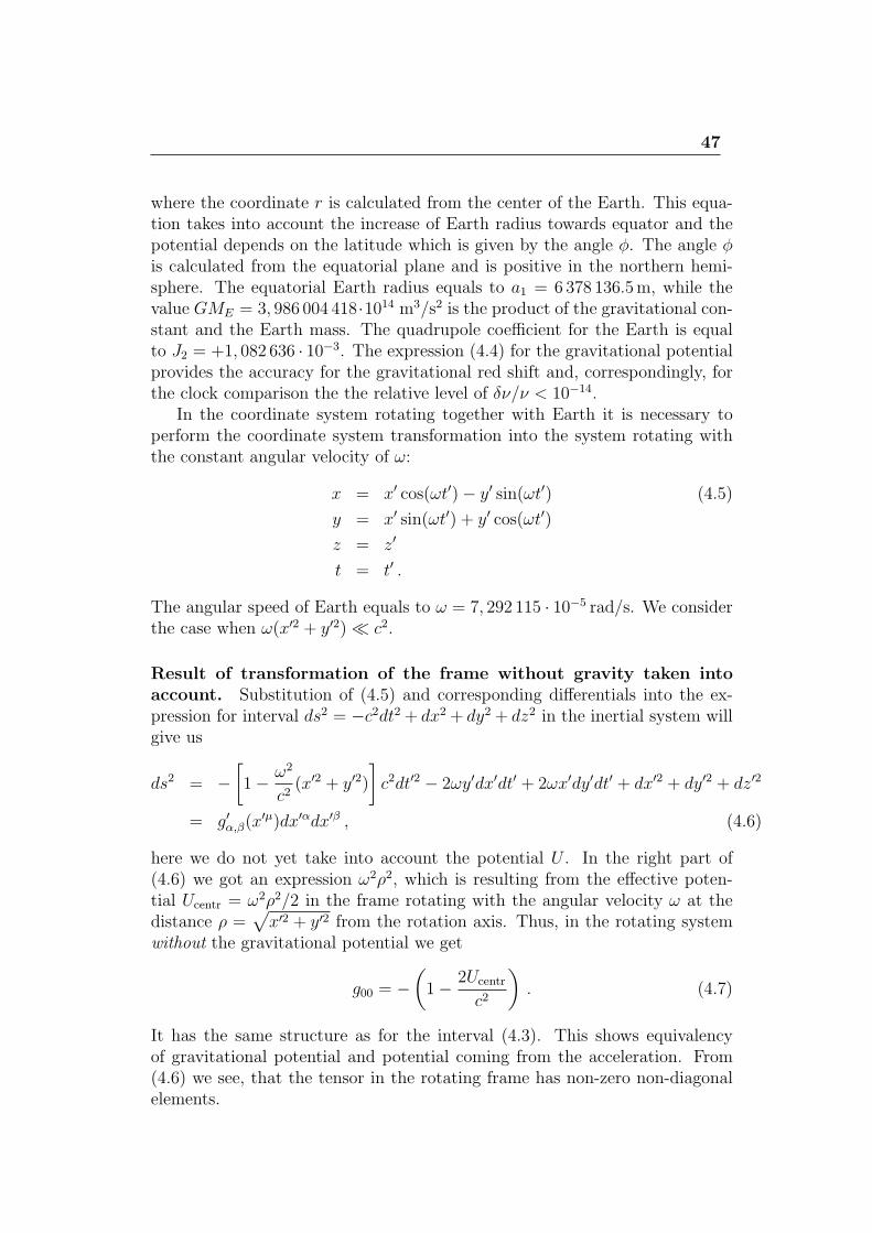
where the coordinate r is calculated from the center of the Earth. This equa-tion takes into account the increase of Earth radius towards equator and thepotential depends on the latitude which is given by the angle ϕ. The angle ϕis calculated from the equatorial plane and is positive in the northern hemi-sphere. The equatorial Earth radius equals to a1 = 6378 136.5m, while thevalue GME = 3, 986 004 418·1014 m3/s2 is the product of the gravitational con-stant and the Earth mass. The quadrupole coefficient for the Earth is equalto J2 = +1, 082 636 · 10−3. The expression (4.4) for the gravitational potentialprovides the accuracy for the gravitational red shift and, correspondingly, forthe clock comparison the the relative level of δν/ν < 10−14.

In the coordinate system rotating together with Earth it is necessary toperform the coordinate system transformation into the system rotating withthe constant angular velocity of ω:

x = x′ cos(ωt′)− y′ sin(ωt′) (4.5)

y = x′ sin(ωt′) + y′ cos(ωt′)

z = z′

t = t′ .

The angular speed of Earth equals to ω = 7, 292 115 · 10−5 rad/s. We considerthe case when ω(x′2 + y′2) ≪ c2.

Result of transformation of the frame without gravity taken intoaccount. Substitution of (4.5) and corresponding differentials into the ex-pression for interval ds2 = −c2dt2 + dx2 + dy2 + dz2 in the inertial system willgive us

ds2 = −[1− ω2

c2(x′2 + y′2)

]c2dt′2 − 2ωy′dx′dt′ + 2ωx′dy′dt′ + dx′2 + dy′2 + dz′2

= g′α,β(x′µ)dx′αdx′β , (4.6)

here we do not yet take into account the potential U . In the right part of(4.6) we got an expression ω2ρ2, which is resulting from the effective poten-tial Ucentr = ω2ρ2/2 in the frame rotating with the angular velocity ω at thedistance ρ =

√x′2 + y′2 from the rotation axis. Thus, in the rotating system

without the gravitational potential we get

g00 = −(1− 2Ucentr

c2

). (4.7)

It has the same structure as for the interval (4.3). This shows equivalencyof gravitational potential and potential coming from the acceleration. From(4.6) we see, that the tensor in the rotating frame has non-zero non-diagonalelements.

48

Rotating frame and gravitational potential For the spherical coordi-nates ( r – distance to the origin, ϕ – latitude and L – angular longitude) thecoordinate transformation looks like

x′ = r cosϕ cosL (4.8)

y′ = r cosϕ sinL

z = r sinϕ

t′ = t ,

and we can get the following expression for the interval:

ds2 = −c2dt2 + [dr2 + r2dϕ2 + r2cos2 ϕ (ω2dt2 + 2ω dLdt+ dL2)] . (4.9)

Compared to (4.2), the metric in the rotating coordinate system with thegravitational potential taken into account can be written as

g00 = −(1− 2U

c2− (ω × r)2

c2

), g0j =

(ω × r)jc

, gij =

(1 +

2U

c2

)δij ,

(4.10)where the vector product of the angular velocity ω and the radius-vector rshowing from the center of Earth towards the observer is equivalent to thecentripetal potential. Non-diagonal elements are responsible for Sagnac effect,which will be considered later.

4.2 Transformation of time: gravitational shift,

time dilation, Sagnac effect

According to SI second definition, time indicated by the clock is so-called localtime τ : The time measured in the coordinate system rigidly connected to theclock. Consider infinitely small transportation of the clock from one point toanother which is described in some external frame by two coordinate points(x0, x1, x2, x3) and (x0 + dt, x1 + dx1, x2 + dx2, x3 + dx3). The interval

dτ =1

c

√−ds2 (4.11)

connects the increment of the local time dτ measured by the clock and theincrement of coordinate time dt of time t, measured in some other, externalframe. Time t is called as coordinate time. The increment of the coordinatetime dt is connected with the increment of the local time by a simple expression

dt = dτdt

dτ, (4.12)

49

which can be calculated using (4.11) at some moment (x0, x1, x2, x3). Inte-gration of (4.12) along the world’s line will give us the coordinate time dt(t).The derivative dτ/dt can be calculated using (4.1) and (4.11) as

dτ

dt=

√−g00(x0, x1, x2, x3)−

2

cg0i(x0, x1, x2, x3)

dxi

dt− 1

c2gij(x0, x1, x2, x3)

dxi

dt

dxj

dt.

(4.13)Close to the Earth’s surface the influence of the gravitational potential on

the metric is small (2U/c2 ≈ 1, 4 · 10−9 ≪ 1). Hence we will consider onlysmall deviation from the flat space using some small parameter h(t)

dτ

dt≡ 1− h(t) , (4.14)

where h(t) is the power series over 1/c. The difference between the coordinateand local time is thus equals to

∆t ≡ t− τ =

∫ t

t0

h(t)dt . (4.15)

The difference ∆t can be calculated either using metric in the geocentric frame(4.3) or in the coordinate system rotating together with Earth (4.9). For themetric in the geocentric non-rotating frame (4.3) the non-diagonal elementsequal to zero and the substitution into (4.13) will give us

h(t) = 1−

√(1− U

2c2

)− 1

c2

(1 +

U

2c2

)v2 . (4.16)

Expanding it in power series we will get

h(t) =U(t)

c2+

v2

2c2+O

(1

c4

). (4.17)

The second part in this expression is known as time dilation or the secondorder Doppler effect for the clock moving with velocity v in respect to theframe. The contribution of O

(1c4

)is typically less than 10−18 and will not be

considered in the future.For the frame, rotating together with Earth, one gets the following expres-

sion

h(t) =1

c2

[Ug +∆U(t) +

V (t)2

2

]+

2ω

c2dAE

dt, (4.18)

which one can get similar to (4.16) using the metric (4.9). Here V (t) – isthe modulus of the coordinate velocity in respect to the Earth. The last partappears due to the Sagnac effect:

1

c2

∫ Q

P(ω × r) · dr = 1

c2

∫ Q

Pω · (r × dr) = 2

1

c2

∫ Q

Pω · dAE =

2ωAE

c2. (4.19)

50

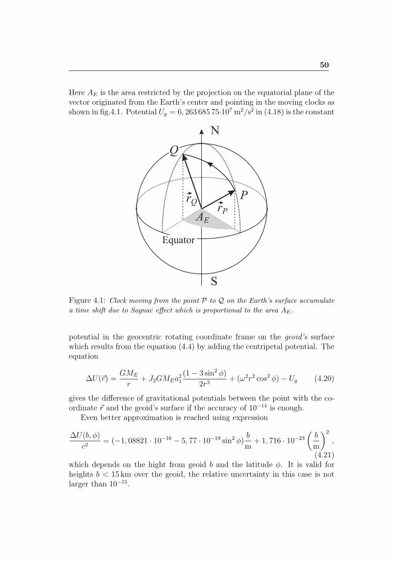
Here AE is the area restricted by the projection on the equatorial plane of thevector originated from the Earth’s center and pointing in the moving clocks asshown in fig.4.1. Potential Ug = 6, 263 685 75·107 m2/s2 in (4.18) is the constant

Figure 4.1: Clock moving from the point P to Q on the Earth’s surface accumulate

a time shift due to Sagnac effect which is proportional to the area AE.

potential in the geocentric rotating coordinate frame on the geoid’s surfacewhich results from the equation (4.4) by adding the centripetal potential. Theequation

∆U(r) =GME

r+ J2GMEa

21

(1− 3 sin2 ϕ)

2r3+ (ω2r2 cos2 ϕ)− Ug (4.20)

gives the difference of gravitational potentials between the point with the co-ordinate r and the geoid’s surface if the accuracy of 10−14 is enough.

Even better approximation is reached using expression

∆U(b, ϕ)

c2= (−1, 08821 · 10−16 − 5, 77 · 10−19 sin2 ϕ)

b

m+ 1, 716 · 10−23

(b

m

)2

,

(4.21)which depends on the hight from geoid b and the latitude ϕ. It is valid forheights b < 15 km over the geoid, the relative uncertainty in this case is notlarger than 10−15.

51

4.3 Time and frequency comparison

First of all, we have to agree about what means synchronization of two clocks.We agree that synchronized clocks give the same reading at the same time.Today one uses the “coordinate synchronization” when two events describedin some frame by full coordinate sets xµ1 and xµ2 correspondingly are consideredas simultaneous if the time coordinates are equal (x01 = x02).

One can compare two clocks placed at different positions on the Earth’ssurface P , Q by different means. Till some time the most regular methodused the physical transportation, now the exchange of electromagnetic signalsis widely used. Both these processes are described earlier mathematically inthe geocentric frame. The frame can be chosen either using (i) the inertialframe with fixed direction of axes (e.g. pointing on distant quasars/stars) andthe origin having the same instant velocity as Earth or (ii) the rotating frame.Equations will depend on the selected frame.

4.3.1 Comparing of transportable clock

If signal is transferred from point P to point Q using a transportable clock,the time difference in the non-rotating geocentric frame is equal to

∆t =

∫ Q

Pds

[1 +

U(r)− Ug

c2+

v2

2c2

]. (4.22)

Here U(r) is the gravitational potential (only) at the clock position, v – theclock speed in a non-rotating geocentric frame, ds – the increment of the localdistance in the clock frame.

In the rotating geocentric frame the time difference will be equal to

∆t =

∫ Q

Pds

[1 +

∆U(r)

c2+V 2

2c2

]+

2ω

c2AE , (4.23)

where V is the clock speed in respect to the Earth surface. Vector r is pointingclocks during transportation from P to Q. The vector projection r on theequatorial plane restricts the area AE.

Three last terms in the (4.23) are the results of gravitation, time dilationand Sagnac effect. The latter results from the fact that clock and Earth arerotating with the same angular velocity. It means that the speed a non-rotationframe will depend on the latitude which defines the distance to the Earth’s axis.The area AE is considered as positive if clock are moving to the East. Situationshown in fig. 4.1 corresponds to the negative AE.

4.3.2 Transfer using electromagnetic signals

For comparison of two separated clocks with the help of electromagnetic signalsof radio- or optical frequency there exist basically three methods of different

52

complexity: (i) one-way transfer, (ii) differential method and (iii) differentialmethod.

Time passing between emission and receiving of electromagnetic signal ina non-rotating geocentric frame equals to

∆t =1

c

∫ Q

Pdσ

[1 +

U(r)− Ug

c2+

v2

2c2

], (4.24)

where dσ is the increment of local distance between points P and Q, all othervalues are the same as in (4.22).

In the rotating frame we will get

∆t =1

c

∫ Q

Pdσ

[1 +

∆U(r)

c2

]+

2ω

c2AE , (4.25)

where ∆U(r) is the gravitational potential in the point r reduced by the geoid’spotential in the coordinate system rotating with Earth and AE – the equatorialprojection area.

In the case if the signal is transmitted to the satellite at the geostation-ary orbit, the second term ∆U(r) results in the correction of about the 1ns corresponding to the distance of ct ≃ 30 cm. The third term containing2ω/c2 = 1, 6227 · 10−6 ns/km2 can reach hundreds of nanoseconds.

One-way transfer

The simplest way of time and frequency transfer is the transmission of codedsignals. The simplest examples is are the time got by phone, TV or the In-ternet. Radio-frequency transmitters of the short- and long wave range coverlarge areas where the receiver can get sufficient signal. On-board clocks atGPS satellites allow to receive accurate time signal over the whole globe.

The accuracy which can be achieved using this method depends on thepropagation time and can reach a few tenths of a second if one uses the Internetline or satellite signal. This error can be significantly reduced if the client sendsthe signal back and the provider of time signal can measure the whole delayin the line client-server-client. Assuming that the delays in both propagationdirections are the same, one can introduce the correction and compensate thesignificant part of the original error. For the satellite one can calculate thecorrection from the time distance to the satellite divided by speed of light

Differential method

Signal distributed by one source and received by two or more clients simulta-neously can be used for client’s clock synchronization. E.g. two users on theEarth’s surface can use a signal from one satellite to synchronize their clocks.Consider two stations, A and B receiving the signal tS propagating by two

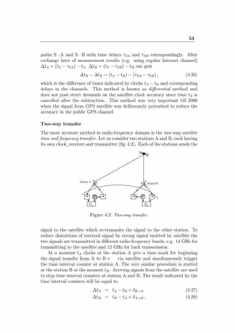
53

paths S –A and S –B with time delays τSA and τSB correspondingly. Afterexchange later of measurement results (e.g. using regular Internet channel)∆tA = (tS − τSA)− tA ∆tB = (tS − τSB)− tB one gets

∆tB −∆tB = (tA − tB)− (τSA − τSB) , (4.26)

which is the difference of times indicated by clocks tA − tB and correspondingdelays in the channels. This method is known as differential method anddoes not pose strict demands on the satellite clock accuracy since time tS iscancelled after the subtraction. This method was very important till 2000when the signal from GPS satellite was deliberately perturbed to reduce theaccuracy in the public GPS channel.

Two-way transfer

The most accurate method in radio-frequency domain is the two-way satellitetime and frequency transfer. Let us consider two stations A and B, each havingits own clock, receiver and transmitter (fig. 4.2). Each of the stations sends the

Figure 4.2: Two-way transfer.

signal to the satellite which re-transmits the signal to the other station. Toreduce distortions of received signal by strong signal emitted by satellite thetwo signals are transmitted in different radio-frequency bands, e.g. 14 GHz fortransmitting to the satellite and 12 GHz for back transmission.

At a moment tA clocks at the station A give a time mark for beginningthe signal transfer from A to B v via satellite and simultaneously triggerthe time interval counter at station A. The very similar procedure is startedat the station B at the moment tB. Arriving signals from the satellite are usedto stop time interval counters at station A and B. The result indicated by thetime interval counters will be equal to

∆tA = tA − tB + δB→A (4.27)

∆tB = tB − tA + δA→B . (4.28)

54

If both directions are fully equivalent, the delays δB→A δA→B are the same.The time difference of the clocks at stations A and B ∆T can be calculatedafter both stations will exchange the measurement results. By subtracting(4.28) from (4.27), we get ∆T = (∆tA −∆tB)/2.

Still, there are effects which can cause difference in propagation time fortwo directions. For that case the time difference will be equal to:

∆T =∆tA −∆tB

2+

(τupA + τdownB )− (τupB + τdown

A )

2+τA→B − τB→A

2

+(τTA − τRB )− (τTB − τRA )

2+ ∆τR . (4.29)

The first term (∆tA−∆tB)/2 is the measured time difference, while the secondterm [(τupA + τdown

B )− (τupB + τdownA )]/2 is the contribution from delays in one

and the other direction. If the signal transfer occurs approximately at the samemoment, the second term can be neglected. The third term takes into accountdifference in the delays of the satellite re-translation device and is typicallyinsignificant. The fourth contribution in (4.29) is the difference of time delaysfor signal transmission in the receiver and translator themselves. The last term∆τR is the Sagnac effect which takes into account the Earth rotation.

4.3.3 Transfer of optical frequencies

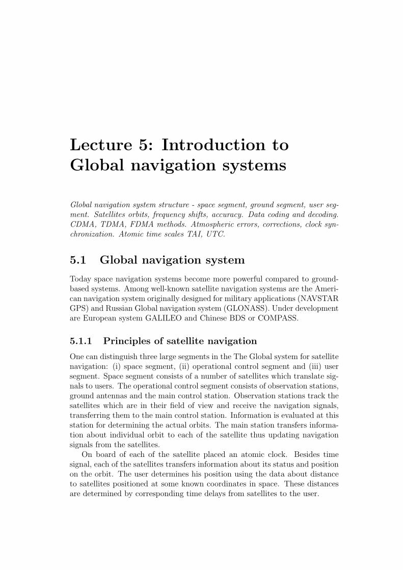
Lecture 5: Introduction toGlobal navigation systems

Global navigation system structure - space segment, ground segment, user seg-ment. Satellites orbits, frequency shifts, accuracy. Data coding and decoding.CDMA, TDMA, FDMA methods. Atmospheric errors, corrections, clock syn-chronization. Atomic time scales TAI, UTC.

5.1 Global navigation system

Today space navigation systems become more powerful compared to ground-based systems. Among well-known satellite navigation systems are the Ameri-can navigation system originally designed for military applications (NAVSTARGPS) and Russian Global navigation system (GLONASS). Under developmentare European system GALILEO and Chinese BDS or COMPASS.

5.1.1 Principles of satellite navigation

One can distinguish three large segments in the The Global system for satellitenavigation: (i) space segment, (ii) operational control segment and (iii) usersegment. Space segment consists of a number of satellites which translate sig-nals to users. The operational control segment consists of observation stations,ground antennas and the main control station. Observation stations track thesatellites which are in their field of view and receive the navigation signals,transferring them to the main control station. Information is evaluated at thisstation for determining the actual orbits. The main station transfers informa-tion about individual orbit to each of the satellite thus updating navigationsignals from the satellites.

On board of each of the satellite placed an atomic clock. Besides timesignal, each of the satellites transfers information about its status and positionon the orbit. The user determines his position using the data about distanceto satellites positioned at some known coordinates in space. These distancesare determined by corresponding time delays from satellites to the user.

56

For determining position on the Earth surface a GNSS receiver uses timemarks from different satellites and compares them with local built-in clock.If a signal from some satellite “ i ” having coordinates xi, yi, zi was receivedby the user having coordinates X, Y, Z (fig. 5.1), the time delay between theemission and receiving of the signal will define the distance from the satelliteto the user.

If a clock in the receiver and clocks at satellites are perfectly synchronized,the distance to the satellite can be calculated form the propagation time delay∆t1 R1 = c ·∆t1. Measurement of distance to the second satellite will give theposition of the receiver in the common plane. This position will be given by theintersection point of two circles with radii R1 and R2 as shown in fig. 5.1. Forpositioning in the 3D space one needs the third satellite. But, in general caseclocks at receiver is not synchronized with on-board atomic clock. The errorof time synchronization of δt = 1µs will result in the systematic positioningerror of 300m. In the two-dimensional case shown in fig. 5.1 it is implied thattime TU of receiver clock is faster than the navigation system time TGNSS byδtu = TU −TGNSS. The measured distances will increase by c ·δtu which resultsin a wrong measurement of U ′ coordinate. Distances, calculated he signalincluding the clock uncertainty δtu is called“pseudo-distance” Pi = Ri+ c · δtu.

Composing 4 equations containing four different pseudo-distances, one canfour unknown values: three space coordinates X, Y , Z and time difference δtu:

(x1 −X)2 + (y1 − Y )2 + (z1 − Z)2 = (P1 − c δtu)2 ,

(x2 −X)2 + (y2 − Y )2 + (z2 − Z)2 = (P2 − c δtu)2 ,

(x3 −X)2 + (y3 − Y )2 + (z3 − Z)2 = (P3 − c δtu)2 , (5.1)

(x4 −X)2 + (y4 − Y )2 + (z4 − Z)2 = (P4 − c δtu)2 .

This non-linear system can be solved either by linearization, or in a closed form.The linearized system is obtained from the original one by Taylor expansionand is solved iteratively by substituting initial expected values for coordinatesand time difference. Usually GNSS uses a reference ellipsoid for geocentricWorld system WGS84.

Further we give more detailed description of typical GPS characteristics,taking into account that other systems operate using similar principles.

5.1.2 GPS system operation

Clocks on board of GPS satellites are synchronized in respect to UTC(USNO)and the GPS systems distributes the time signal which is an approximationto UTC. GPS time scale is relied on readings of a number of atomic clock onboard of the satellites and ground stations which are combined by a specialprocedure. This scale is corrected by an operational control segment in respectto UTC (USNO) of the US Naval observatory within maximal deviation of 1µs.

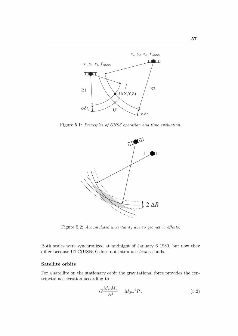
57

Figure 5.1: Principles of GNSS operation and time evaluation.

Figure 5.2: Accumulated uncertainty due to geometric effects.

Both scales were synchronized at midnight of January 6 1980, but now theydiffer because UTC(USNO) does not introduce leap seconds.

Satellite orbits

For a satellite on the stationary orbit the gravitational force provides the cen-tripetal acceleration according to :

GMEMS

R2=MSω

2R . (5.2)

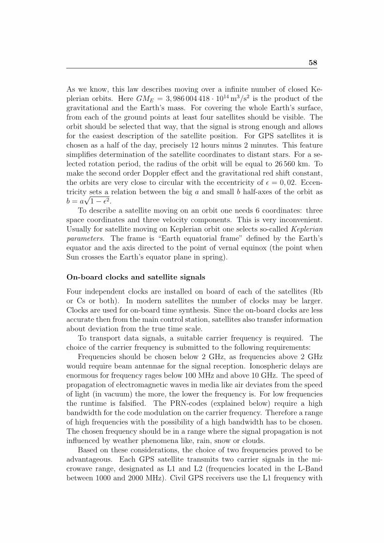
58

As we know, this law describes moving over a infinite number of closed Ke-plerian orbits. Here GME = 3, 986 004 418 · 1014m3/s2 is the product of thegravitational and the Earth’s mass. For covering the whole Earth’s surface,from each of the ground points at least four satellites should be visible. Theorbit should be selected that way, that the signal is strong enough and allowsfor the easiest description of the satellite position. For GPS satellites it ischosen as a half of the day, precisely 12 hours minus 2 minutes. This featuresimplifies determination of the satellite coordinates to distant stars. For a se-lected rotation period, the radius of the orbit will be equal to 26 560 km. Tomake the second order Doppler effect and the gravitational red shift constant,the orbits are very close to circular with the eccentricity of ϵ = 0, 02. Eccen-tricity sets a relation between the big a and small b half-axes of the orbit asb = a

√1− ϵ2.

To describe a satellite moving on an orbit one needs 6 coordinates: threespace coordinates and three velocity components. This is very inconvenient.Usually for satellite moving on Keplerian orbit one selects so-called Keplerianparameters. The frame is “Earth equatorial frame” defined by the Earth’sequator and the axis directed to the point of vernal equinox (the point whenSun crosses the Earth’s equator plane in spring).

On-board clocks and satellite signals

Four independent clocks are installed on board of each of the satellites (Rbor Cs or both). In modern satellites the number of clocks may be larger.Clocks are used for on-board time synthesis. Since the on-board clocks are lessaccurate then from the main control station, satellites also transfer informationabout deviation from the true time scale.

To transport data signals, a suitable carrier frequency is required. Thechoice of the carrier frequency is submitted to the following requirements:

Frequencies should be chosen below 2 GHz, as frequencies above 2 GHzwould require beam antennae for the signal reception. Ionospheric delays areenormous for frequency rages below 100 MHz and above 10 GHz. The speed ofpropagation of electromagnetic waves in media like air deviates from the speedof light (in vacuum) the more, the lower the frequency is. For low frequenciesthe runtime is falsified. The PRN-codes (explained below) require a highbandwidth for the code modulation on the carrier frequency. Therefore a rangeof high frequencies with the possibility of a high bandwidth has to be chosen.The chosen frequency should be in a range where the signal propagation is notinfluenced by weather phenomena like, rain, snow or clouds.

Based on these considerations, the choice of two frequencies proved to beadvantageous. Each GPS satellite transmits two carrier signals in the mi-crowave range, designated as L1 and L2 (frequencies located in the L-Bandbetween 1000 and 2000 MHz). Civil GPS receivers use the L1 frequency with

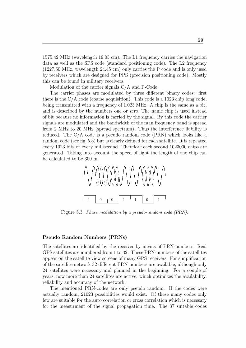
59

1575.42 MHz (wavelength 19.05 cm). The L1 frequency carries the navigationdata as well as the SPS code (standard positioning code). The L2 frequency(1227.60 MHz, wavelength 24.45 cm) only carries the P code and is only usedby receivers which are designed for PPS (precision positioning code). Mostlythis can be found in military receivers.

Modulation of the carrier signals C/A and P-CodeThe carrier phases are modulated by three different binary codes: first

there is the C/A code (coarse acquisition). This code is a 1023 chip long code,being transmitted with a frequency of 1.023 MHz. A chip is the same as a bit,and is described by the numbers one or zero. The name chip is used insteadof bit because no information is carried by the signal. By this code the carriersignals are modulated and the bandwidth of the man frequency band is spreadfrom 2 MHz to 20 MHz (spread spectrum). Thus the interference liability isreduced. The C/A code is a pseudo random code (PRN) which looks like arandom code (see fig. 5.3) but is clearly defined for each satellite. It is repeatedevery 1023 bits or every millisecond. Therefore each second 1023000 chips aregenerated. Taking into account the speed of light the length of one chip canbe calculated to be 300 m.

Figure 5.3: Phase modulation by a pseudo-random code (PRN).

Pseudo Random Numbers (PRNs)

The satellites are identified by the receiver by means of PRN-numbers. RealGPS satellites are numbered from 1 to 32. These PRN-numbers of the satellitesappear on the satellite view screens of many GPS receivers. For simplificationof the satellite network 32 different PRN-numbers are available, although only24 satellites were necessary and planned in the beginning. For a couple ofyears, now more than 24 satellites are active, which optimizes the availability,reliability and accuracy of the network.

The mentioned PRN-codes are only pseudo random. If the codes wereactually random, 21023 possibilities would exist. Of these many codes onlyfew are suitable for the auto correlation or cross correlation which is necessaryfor the measurment of the signal propagation time. The 37 suitable codes

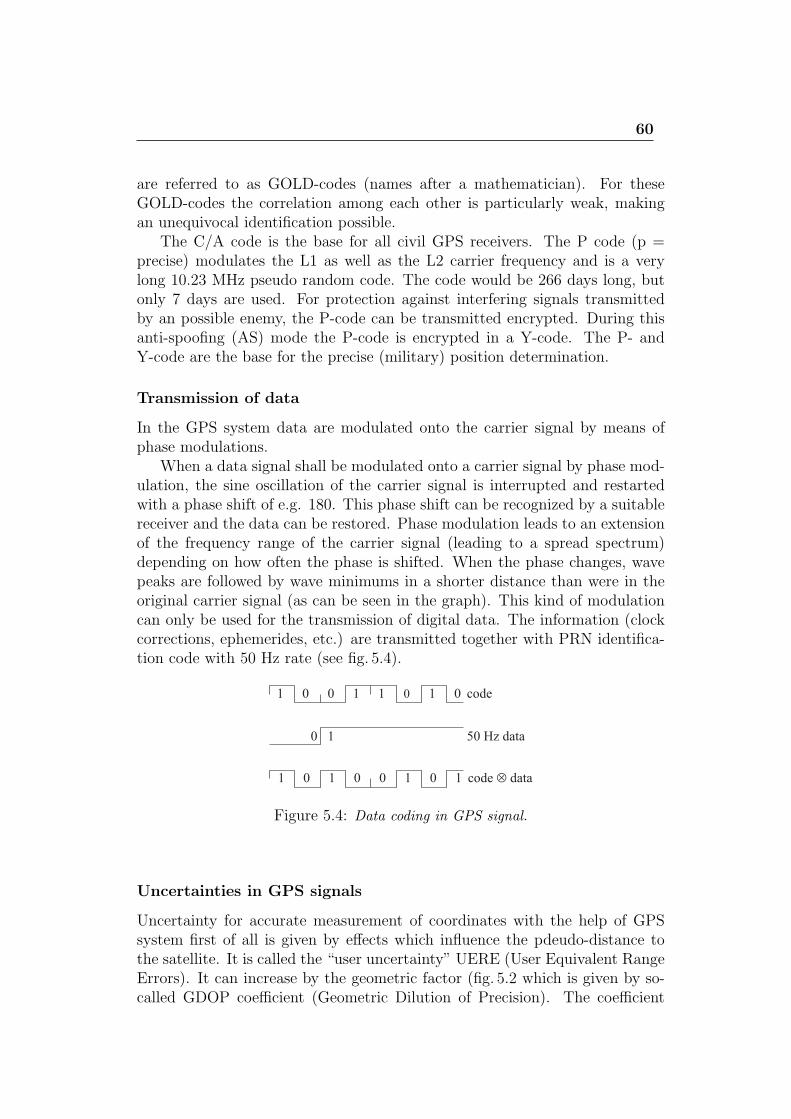
60

are referred to as GOLD-codes (names after a mathematician). For theseGOLD-codes the correlation among each other is particularly weak, makingan unequivocal identification possible.

The C/A code is the base for all civil GPS receivers. The P code (p =precise) modulates the L1 as well as the L2 carrier frequency and is a verylong 10.23 MHz pseudo random code. The code would be 266 days long, butonly 7 days are used. For protection against interfering signals transmittedby an possible enemy, the P-code can be transmitted encrypted. During thisanti-spoofing (AS) mode the P-code is encrypted in a Y-code. The P- andY-code are the base for the precise (military) position determination.

Transmission of data

In the GPS system data are modulated onto the carrier signal by means ofphase modulations.

When a data signal shall be modulated onto a carrier signal by phase mod-ulation, the sine oscillation of the carrier signal is interrupted and restartedwith a phase shift of e.g. 180. This phase shift can be recognized by a suitablereceiver and the data can be restored. Phase modulation leads to an extensionof the frequency range of the carrier signal (leading to a spread spectrum)depending on how often the phase is shifted. When the phase changes, wavepeaks are followed by wave minimums in a shorter distance than were in theoriginal carrier signal (as can be seen in the graph). This kind of modulationcan only be used for the transmission of digital data. The information (clockcorrections, ephemerides, etc.) are transmitted together with PRN identifica-tion code with 50 Hz rate (see fig. 5.4).

Figure 5.4: Data coding in GPS signal.

Uncertainties in GPS signals

Uncertainty for accurate measurement of coordinates with the help of GPSsystem first of all is given by effects which influence the pdeudo-distance tothe satellite. It is called the “user uncertainty” UERE (User Equivalent RangeErrors). It can increase by the geometric factor (fig. 5.2 which is given by so-called GDOP coefficient (Geometric Dilution of Precision). The coefficient

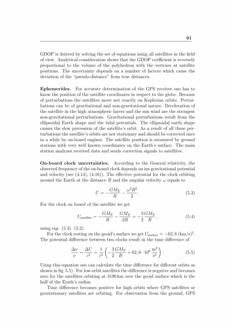
61

GDOP is derived by solving the set of equations using all satellites in the fieldof view. Analytical consideration shows that the GDOP coefficient is reverselyproportional to the volume of the polyhedron with the vertexes at satellitepositions. The uncertainty depends on a number of factors which cause thedeviation of the “pseudo-distance” from true distances.

Ephemerides. For accurate determination of the GPS receiver one has toknow the position of the satellite coordinates in respect to the globe. Becauseof perturbations the satellites move not exactly on Keplerian orbits. Pertur-bations can be of gravitational and non-gravitational nature. Deceleration ofthe satellite in the high atmospheric layers and the sun wind are the strongestnon-gravitational perturbations. Gravitational perturbations result from theellipsoidal Earth shape and the tidal potentials. The ellipsoidal earth shapecauses the slow precession of the satellite’s orbit. As a result of all these per-turbations the satellite’s orbits are not stationary and should be corrected oncein a while by on-board engines. The satellite position is measured by groundstations with very well known coordinates on the Earth’s surface. The mainstation analyzes received data and sends correction signals to satellites.

On-board clock uncertainties. According to the General relativity, theobserved frequency of the on-board clock depends on ins gravitational potentialand velocity (see (4.14), (4.16)). The effective potential for the clock orbitingaround the Earth at the distance R and the angular velocity ω equals to

U = −GME

R− ω2R2

2. (5.3)

For the clock on board of the satellite we get

Usatellite = −GME

R− GME

2R= −3

2

GME

R, (5.4)

using eqs. (5.3) (5.2).For the clock resting on the geoid’s surface we get Usurface = −62, 6 (km/s)2.

The potential difference between two clocks result in the time difference of

∆ν

ν=

∆U

c2=

1

c2

(−3

2

GME

R+ 62, 6 · 106 m

2

s2

). (5.5)

Using this equation one can calculate the time difference for different orbits asshown in fig. 5.5). For low-orbit satellites the difference is negative and becomeszero for the satellites orbiting at 3190 km over the geoid surface which is thehalf of the Erath’s radius.

Time difference becomes positive for high orbits where GPS satellites orgeostationary satellites are orbiting. For observation from the ground, GPS

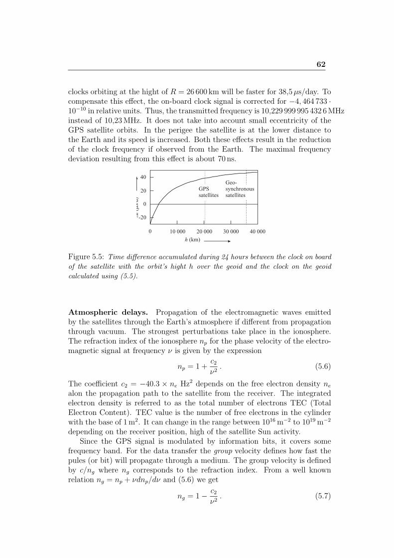
62

clocks orbiting at the hight of R = 26 600 km will be faster for 38,5µs/day. Tocompensate this effect, the on-board clock signal is corrected for −4, 464 733 ·10−10 in relative units. Thus, the transmitted frequency is 10,229 999 995 432 6MHzinstead of 10,23MHz. It does not take into account small eccentricity of theGPS satellite orbits. In the perigee the satellite is at the lower distance tothe Earth and its speed is increased. Both these effects result in the reductionof the clock frequency if observed from the Earth. The maximal frequencydeviation resulting from this effect is about 70 ns.

Figure 5.5: Time difference accumulated during 24 hours between the clock on board

of the satellite with the orbit’s hight h over the geoid and the clock on the geoid

calculated using (5.5).

Atmospheric delays. Propagation of the electromagnetic waves emittedby the satellites through the Earth’s atmosphere if different from propagationthrough vacuum. The strongest perturbations take place in the ionosphere.The refraction index of the ionosphere np for the phase velocity of the electro-magnetic signal at frequency ν is given by the expression

np = 1 +c2ν2. (5.6)

The coefficient c2 = −40.3 × ne Hz2 depends on the free electron density ne

alon the propagation path to the satellite from the receiver. The integratedelectron density is referred to as the total number of electrons TEC (TotalElectron Content). TEC value is the number of free electrons in the cylinderwith the base of 1m2. It can change in the range between 1016 m−2 to 1019 m−2

depending on the receiver position, high of the satellite Sun activity.Since the GPS signal is modulated by information bits, it covers some

frequency band. For the data transfer the group velocity defines how fast thepules (or bit) will propagate through a medium. The group velocity is definedby c/ng where ng corresponds to the refraction index. From a well knownrelation ng = np + νdnp/dν and (5.6) we get

ng = 1− c2ν2. (5.7)

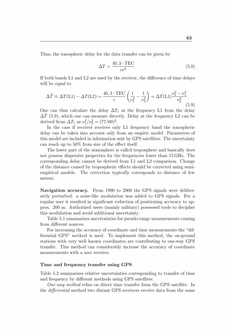
63

Thus, the ionospheric delay for the data transfer can be given by

∆T =40, 3 · TEC

cν2. (5.8)

If both bands L1 and L2 are used by the receiver, the difference of time delayswill be equal to

∆T ≡ ∆T (L1)−∆T (L2) =40, 3 · TEC

c

(1

ν21− 1

ν22

)= ∆T (L1)

ν22 − ν21ν22

.

(5.9)One can thus calculate the delay ∆T1 at the frequency L1 from the delay∆T (5.9), which one can measure directly. Delay at the frequency L2 can bederived from ∆T1 as ν21/ν

22 = (77/60)2.

In the case if receiver receives only L1 frequency band the ionosphericdelay can be taken into account only from an empiric model. Parameters ofthis model are included in information sent by GPS satellites. The uncertaintycan reach up to 50% from size of the effect itself.

The lower part of the atmosphere is called troposphere and basically doesnot possess dispersive properties for the frequencies lower than 15GHz. Thecorresponding delay cannot be derived from L1 and L2 comparison. Changeof the distance caused by tropospheric effects should be corrected using semi-empirical models. The correction typically corresponds to distance of fewmeters.

Navigation accuracy. From 1990 to 2000 the GPS signals were deliber-ately perturbed: a noise-like modulation was added to GPS signals. For aregular user it resulted in significant reduction of positioning accuracy to ap-prox. 200 m. Authorized users (mainly military) possessed tools to decipherthis modulation and avoid additional uncertainty.

Table 5.1 summarizes uncertainties for pseudo-range measurements comingfrom different sources.

For increasing the accuracy of coordinate and time measurements the “dif-ferential GPS” method is used. To implement this method, the on-groundstations with very well known coordinates are contributing to one-way GPStransfer. This method can considerably increase the accuracy of coordinatemeasurements with a user receiver.

Time and frequency transfer using GPS

Table 5.2 summarizes relative uncertainties corresponding to transfer of timeand frequency by different methods using GPS satellites.

One-way method relies on direct time transfer form the GPS satellite. Inthe differential method two distant GPS receivers receive data from the same

64

Source of uncertainty uncertaintyon-board clocks 3,0msatellite orbits 1,0mother perturbations 0,5mephemerides prediction 4,2mother 0,9mionospheric delay 2,3mtropospheric delay 2,0mreceiver nose 1,5mpropagation 1,2mby different channelsothers 0,5msum 6,6m

Table 5.1: Uncertainties for pseudo-range measurements (status 2006) for thespace segment, control segment and user segment.

method relativetime uncertainty frequencys uncertainty

one-way <20 ns < 2 · 10−13

one-channel ≈10 ns ≈ 10−13

differential

multi-channel < 5 ns < 5 · 10−14

differential

differential with < 500 ps < 5 · 10−15

carrier phase measurement

Table 5.2: Uncertainties at the level of 2σ for GPS measurements for 24 hraveraging time.

satellite simultaneously. For improving uncertainty one can implement car-rier phase measurement. Usually the complicated geodesic receivers get allinformation about channels PA, P1, P2 as well as L1 and L2 phase.

For sub-nanosecond accuracies one needs to now the distance between an-tenna and the receiver with a very high accuracy (1 m is equivalent to 5 ns).

The accuracy of time transfer (status 2001) can be evaluated from the plotfig. 5.6. The main uncertainty comes from GPS (standard deviation approx.2,6 ns) (TWSTFT) GPS.

65

Figure 5.6: The difference between time measurements at PTB and NPL for TW-

STFT (two-way transfer) and differential GPS method (code C/A). The result shows

full-day measurements for certain Julian days ( MJD=0 corresponds to 0 o’clock

17November 1858. )

5.2 Code division multiplexing (Synchronous

CDMA)

CDMA is a spread spectrum multiple access[6] technique. A spread spectrumtechnique spreads the bandwidth of the data uniformly for the same trans-mitted power. A spreading code is a pseudo-random code that has a narrowambiguity function, unlike other narrow pulse codes.

Each user in a CDMA system uses a different code to modulate their sig-nal. Choosing the codes used to modulate the signal is very important in theperformance of CDMA systems. The best performance will occur when thereis good separation between the signal of a desired user and the signals of otherusers. The separation of the signals is made by correlating the received signalwith the locally generated code of the desired user. If the signal matches thedesired user’s code then the correlation function will be high and the systemcan extract that signal. If the desired user’s code has nothing in common withthe signal the correlation should be as close to zero as possible (thus eliminat-ing the signal); this is referred to as cross correlation. If the code is correlatedwith the signal at any time offset other than zero, the correlation should be asclose to zero as possible. This is referred to as auto-correlation and is used toreject multi-path interference.

An analogy to the problem of multiple access is a room (channel) in whichpeople wish to talk to each other simultaneously. To avoid confusion, peoplecould take turns speaking (time division), speak at different pitches (frequencydivision), or speak in different languages (code division). CDMA is analogousto the last example where people speaking the same language can understandeach other, but other languages are perceived as noise and rejected. Similarly,

66

in radio CDMA, each group of users is given a shared code. Many codesoccupy the same channel, but only users associated with a particular code cancommunicate.

Synchronous CDMA exploits mathematical properties of orthogonality be-tween vectors representing the data strings. For example, binary string 1011is represented by the vector (1, 0, 1, 1). Vectors can be multiplied by takingtheir dot product, by summing the products of their respective components(for example, if u = (a, b) and v = (c, d), then their dot product u·v = ac+bd).If the dot product is zero, the two vectors are said to be orthogonal to eachother. Some properties of the dot product aid understanding of how W-CDMAworks. If vectors a and b are orthogonal, then a · b = 0 .

5.2.1 Example

Start with a set of vectors that are mutually orthogonal. (Although mutualorthogonality is the only condition, these vectors are usually constructed forease of decoding, for example columns or rows from Walsh matrices.) Anexample of orthogonal functions is shown in the picture on the left. Thesevectors will be assigned to individual users and are called the code, chip code,or chipping code. In the interest of brevity, the rest of this example usescodes,v, with only 2 bits.

Walsh matirces

H(21) =

[1 11 −1

],

H(22) =

1 1 1 11 −1 1 −11 1 −1 −11 −1 −1 1

,and in general

H(2k) =

[H(2k−1) H(2k−1)H(2k−1) −H(2k−1)

]= H(2)⊗H(2k−1).

Each user is associated with a different code, say v. A 1 bit is representedby transmitting a positive code,v, and a 0 bit is represented by a negativecode, v. For example, if v = (v0, v1) = (1, 1) and the data that the user wishesto transmit is (1, 0, 1, 1), then the transmitted symbols would be (v, v, v, v) =(v0, v1, v0, v1, v0, v1, v0, v1) = (1, 1, 1, 1, 1, 1, 1, 1).

Each sender has a different, unique vector v chosen from that set, but theconstruction method of the transmitted vector is identical.

Now, due to physical properties of interference, if two signals at a pointare in phase, they add to give twice the amplitude of each signal, but if theyare out of phase, they subtract and give a signal that is the difference of theamplitudes. Digitally, this behavior can be modelled by the addition of thetransmission vectors, component by component.

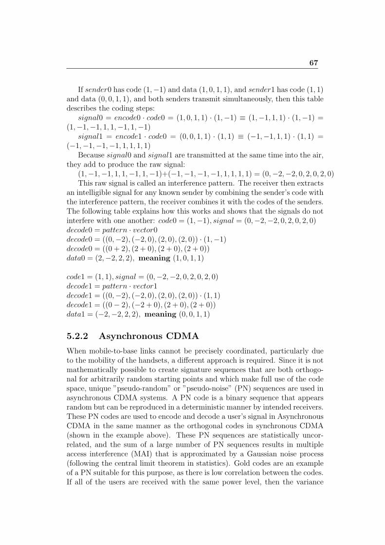
67

If sender0 has code (1,−1) and data (1, 0, 1, 1), and sender1 has code (1, 1)and data (0, 0, 1, 1), and both senders transmit simultaneously, then this tabledescribes the coding steps:

signal0 = encode0 · code0 = (1, 0, 1, 1) · (1,−1) ≡ (1,−1, 1, 1) · (1,−1) =(1,−1,−1, 1, 1,−1, 1,−1)

signal1 = encode1 · code0 = (0, 0, 1, 1) · (1, 1) ≡ (−1,−1, 1, 1) · (1, 1) =(−1,−1,−1,−1, 1, 1, 1, 1)

Because signal0 and signal1 are transmitted at the same time into the air,they add to produce the raw signal:

(1,−1,−1, 1, 1,−1, 1,−1)+(−1,−1,−1,−1, 1, 1, 1, 1) = (0,−2,−2, 0, 2, 0, 2, 0)This raw signal is called an interference pattern. The receiver then extracts

an intelligible signal for any known sender by combining the sender’s code withthe interference pattern, the receiver combines it with the codes of the senders.The following table explains how this works and shows that the signals do notinterfere with one another: code0 = (1,−1), signal = (0,−2,−2, 0, 2, 0, 2, 0)decode0 = pattern · vector0decode0 = ((0,−2), (−2, 0), (2, 0), (2, 0)) · (1,−1)decode0 = ((0 + 2), (2 + 0), (2 + 0), (2 + 0))data0 = (2,−2, 2, 2), meaning (1, 0, 1, 1)

code1 = (1, 1), signal = (0,−2,−2, 0, 2, 0, 2, 0)decode1 = pattern · vector1decode1 = ((0,−2), (−2, 0), (2, 0), (2, 0)) · (1, 1)decode1 = ((0− 2), (−2 + 0), (2 + 0), (2 + 0))data1 = (−2,−2, 2, 2), meaning (0, 0, 1, 1)

5.2.2 Asynchronous CDMA

When mobile-to-base links cannot be precisely coordinated, particularly dueto the mobility of the handsets, a different approach is required. Since it is notmathematically possible to create signature sequences that are both orthogo-nal for arbitrarily random starting points and which make full use of the codespace, unique ”pseudo-random” or ”pseudo-noise” (PN) sequences are used inasynchronous CDMA systems. A PN code is a binary sequence that appearsrandom but can be reproduced in a deterministic manner by intended receivers.These PN codes are used to encode and decode a user’s signal in AsynchronousCDMA in the same manner as the orthogonal codes in synchronous CDMA(shown in the example above). These PN sequences are statistically uncor-related, and the sum of a large number of PN sequences results in multipleaccess interference (MAI) that is approximated by a Gaussian noise process(following the central limit theorem in statistics). Gold codes are an exampleof a PN suitable for this purpose, as there is low correlation between the codes.If all of the users are received with the same power level, then the variance

68

(e.g., the noise power) of the MAI increases in direct proportion to the numberof users. In other words, unlike synchronous CDMA, the signals of other userswill appear as noise to the signal of interest and interfere slightly with thedesired signal in proportion to number of users.

5.2.3 Flexible allocation of resources

Asynchronous CDMA offers a key advantage in the flexible allocation of re-sources i.e. allocation of a PN codes to active users. In the case of CDM(synchronous CDMA), TDMA, and FDMA the number of simultaneous or-thogonal codes, time slots and frequency slots respectively are fixed hence thecapacity in terms of number of simultaneous users is limited. There are a fixednumber of orthogonal codes, time slots or frequency bands that can be allo-cated for CDM, TDMA, and FDMA systems, which remain underutilized dueto the bursty nature of telephony and packetized data transmissions. There isno strict limit to the number of users that can be supported in an asynchronousCDMA system, only a practical limit governed by the desired bit error prob-ability, since the SIR (Signal to Interference Ratio) varies inversely with thenumber of users. In a bursty traffic environment like mobile telephony, theadvantage afforded by asynchronous CDMA is that the performance (bit errorrate) is allowed to fluctuate randomly, with an average value determined bythe number of users times the percentage of utilization. Suppose there are 2Nusers that only talk half of the time, then 2N users can be accommodated withthe same average bit error probability as N users that talk all of the time. Thekey difference here is that the bit error probability for N users talking all ofthe time is constant, whereas it is a random quantity (with the same mean)for 2N users talking half of the time.

In other words, asynchronous CDMA is ideally suited to a mobile networkwhere large numbers of transmitters each generate a relatively small amount oftraffic at irregular intervals. CDM (synchronous CDMA), TDMA, and FDMAsystems cannot recover the underutilized resources inherent to bursty trafficdue to the fixed number of orthogonal codes, time slots or frequency channelsthat can be assigned to individual transmitters. For instance, if there are Ntime slots in a TDMA system and 2N users that talk half of the time, then halfof the time there will be more than N users needing to use more than N timeslots. Furthermore, it would require significant overhead to continually allocateand deallocate the orthogonal code, time slot or frequency channel resources.By comparison, asynchronous CDMA transmitters simply send when they havesomething to say, and go off the air when they don’t, keeping the same PNsignature sequence as long as they are connected to the system.

69

5.2.4 Spread-spectrum characteristics of CDMA

Most modulation schemes try to minimize the bandwidth of this signal sincebandwidth is a limited resource. However, spread spectrum techniques usea transmission bandwidth that is several orders of magnitude greater thanthe minimum required signal bandwidth. One of the initial reasons for doingthis was military applications including guidance and communication systems.These systems were designed using spread spectrum because of its security andresistance to jamming. Asynchronous CDMA has some level of privacy builtin because the signal is spread using a pseudo-random code; this code makesthe spread spectrum signals appear random or have noise-like properties. Areceiver cannot demodulate this transmission without knowledge of the pseudo-random sequence used to encode the data. CDMA is also resistant to jamming.A jamming signal only has a finite amount of power available to jam the signal.The jammer can either spread its energy over the entire bandwidth of the signalor jam only part of the entire signal.

CDMA can also effectively reject narrow band interference. Since narrowband interference affects only a small portion of the spread spectrum signal, itcan easily be removed through notch filtering without much loss of information.Convolution encoding and interleaving can be used to assist in recovering thislost data. CDMA signals are also resistant to multipath fading. Since thespread spectrum signal occupies a large bandwidth only a small portion of thiswill undergo fading due to multipath at any given time. Like the narrow bandinterference this will result in only a small loss of data and can be overcome.

Another reason CDMA is resistant to multipath interference is becausethe delayed versions of the transmitted pseudo-random codes will have poorcorrelation with the original pseudo-random code, and will thus appear asanother user, which is ignored at the receiver. In other words, as long as themultipath channel induces at least one chip of delay, the multipath signals willarrive at the receiver such that they are shifted in time by at least one chip fromthe intended signal. The correlation properties of the pseudo-random codesare such that this slight delay causes the multipath to appear uncorrelatedwith the intended signal, and it is thus ignored.

Lecture 6: Precisionmeasurements in astrophysics

Pulsars as astrophysical sources of periodic pulses. Physics of pulsars. Pulsarsin double star systems. Drift of perimetrium and General relativity tests. Ra-diation of gravitational waves. Search for drift of the fine structure constant.

Methods of precision time and frequency measurements and clock syn-chronization open new opportunities for cosmological studies, physics of intra-stellar media, study of exaplanetory orbits, etc. In this lecture we will considera few implementations and examples.

6.1 Pulsars and Frequency Standards

In 1967 researchers discovered cosmic objects emitting periodic radio-signalswhich attracted a lot of interest from the community. These objects werecalled “pulsars ”. They emit very broad (from radio frequencies to γ-rays)periodic pulses with intervals from one milliseconds to a few seconds. Thenumber of discovered objects reached more than 1000 in 1998. It was foundout that the time interval τ between pulses was very stable (∆τ/τ ≈ 10−3),the pulses should been emitted by solid bodies. One can assume a spinningbody with a radiofrequency source fixed on its surface with a narrow angularemission pattern. The emitting cone periodically scans Earth similar to thelight projector in lighthouse Fig. 6.1.

For a rigid spinning body on can get a restriction coming from the fact,that the linear speed on it’s surface cannot exceed the speed of light c. If apulsar rotates with a period of 1ms, its radius R cannot exceed 50 km. PulsarPSRB1937+21 has a rotation period of 1.6ms. It is very improbable thatpulsars with shorter period will be discovered. It is due to another relation,connecting the centripetal acceleration and gravitational force at its surface.Using the relation one can set a restriction to the highest angular velocityΩ =

√GM/R3, where G is the gravitational constant, R is the radius and

M = 4πR3ρ/3 is the mass of the body. If we substitute the highest knowndensity ρ which is the neutron star density ρ ≈ 1017 kg/m3 we get the minimalrotation period of 1,2ms. It is considered, that pulsars are the rotating neutron

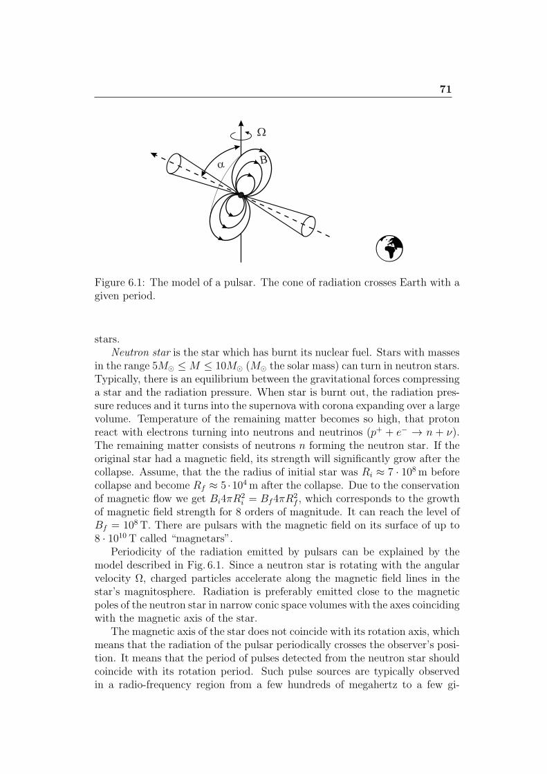
71

Figure 6.1: The model of a pulsar. The cone of radiation crosses Earth with agiven period.

stars.Neutron star is the star which has burnt its nuclear fuel. Stars with masses

in the range 5M⊙ ≤M ≤ 10M⊙ (M⊙ the solar mass) can turn in neutron stars.Typically, there is an equilibrium between the gravitational forces compressinga star and the radiation pressure. When star is burnt out, the radiation pres-sure reduces and it turns into the supernova with corona expanding over a largevolume. Temperature of the remaining matter becomes so high, that protonreact with electrons turning into neutrons and neutrinos (p+ + e− → n + ν).The remaining matter consists of neutrons n forming the neutron star. If theoriginal star had a magnetic field, its strength will significantly grow after thecollapse. Assume, that the the radius of initial star was Ri ≈ 7 · 108m beforecollapse and become Rf ≈ 5 ·104m after the collapse. Due to the conservationof magnetic flow we get Bi4πR

2i = Bf4πR

2f , which corresponds to the growth

of magnetic field strength for 8 orders of magnitude. It can reach the level ofBf = 108T. There are pulsars with the magnetic field on its surface of up to8 · 1010T called “magnetars”.

Periodicity of the radiation emitted by pulsars can be explained by themodel described in Fig. 6.1. Since a neutron star is rotating with the angularvelocity Ω, charged particles accelerate along the magnetic field lines in thestar’s magnitosphere. Radiation is preferably emitted close to the magneticpoles of the neutron star in narrow conic space volumes with the axes coincidingwith the magnetic axis of the star.

The magnetic axis of the star does not coincide with its rotation axis, whichmeans that the radiation of the pulsar periodically crosses the observer’s posi-tion. It means that the period of pulses detected from the neutron star shouldcoincide with its rotation period. Such pulse sources are typically observedin a radio-frequency region from a few hundreds of megahertz to a few gi-

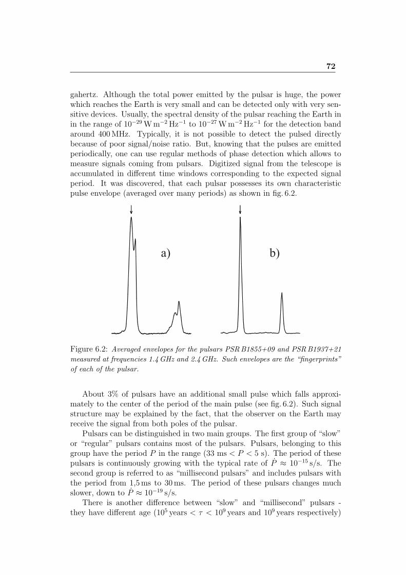
72

gahertz. Although the total power emitted by the pulsar is huge, the powerwhich reaches the Earth is very small and can be detected only with very sen-sitive devices. Usually, the spectral density of the pulsar reaching the Earth inin the range of 10−29Wm−2Hz−1 to 10−27Wm−2Hz−1 for the detection bandaround 400MHz. Typically, it is not possible to detect the pulsed directlybecause of poor signal/noise ratio. But, knowing that the pulses are emittedperiodically, one can use regular methods of phase detection which allows tomeasure signals coming from pulsars. Digitized signal from the telescope isaccumulated in different time windows corresponding to the expected signalperiod. It was discovered, that each pulsar possesses its own characteristicpulse envelope (averaged over many periods) as shown in fig. 6.2.

Figure 6.2: Averaged envelopes for the pulsars PSRB1855+09 and PSRB1937+21

measured at frequencies 1.4GHz and 2.4GHz. Such envelopes are the “fingerprints”

of each of the pulsar.

About 3% of pulsars have an additional small pulse which falls approxi-mately to the center of the period of the main pulse (see fig. 6.2). Such signalstructure may be explained by the fact, that the observer on the Earth mayreceive the signal from both poles of the pulsar.

Pulsars can be distinguished in two main groups. The first group of “slow”or “regular” pulsars contains most of the pulsars. Pulsars, belonging to thisgroup have the period P in the range (33 ms < P < 5 s). The period of thesepulsars is continuously growing with the typical rate of P ≈ 10−15 s/s. Thesecond group is referred to as “millisecond pulsars” and includes pulsars withthe period from 1,5ms to 30ms. The period of these pulsars changes muchslower, down to P ≈ 10−19 s/s.

There is another difference between “slow” and “millisecond” pulsars -they have different age (105 years < τ < 109 years and 109 years respectively)

73

and different strengthes of magnetic field on their surface (B ≈ 108T andB ≈ 104T). About 80% of millisecond pulsars have orbital twins, while for theslow pulsars the fraction of double-stars (pusar+twin) is much less (1%).

Relying on the accepted model describing a pulsar for interpretation ofexperimental data, the pulsar can be treated as a huge classical magnetic dipoleM . The magnetic moment is rotating with the angular frequency Ω and theangle between the magnetic moment and the rotation axis is α. In frames ofclassical electro-dynamics, the rotating magnetic dipole emits radiation withthe power equal to

dE

dt=

2(M sinα)2Ω4

3c2. (6.1)

Emitted power results in deceleration of rotation (the power is taken fromrotation energy)

Erot =1

2ΘΩ2 , (6.2)

where Θ is a moment of inertia of the neutron star. For the sphere of radiusR ≈ 15 km and density of ρ ≈ 1017 kg/m3 it equals to Θ = 2/5MR5 =8/15πρR5 ≈ 1, 3·1038 kgm3. The rate of the energy loss can be calculated fromthe angular velocity of the pulsar Ω = 2π/P and its derivative ω = −2πP/P 2:

dErot

dt= ΘΩΩ = −4π2Θ

P

P 2. (6.3)

For most of the slow pulsars the rate is in the range 1023 W ≤ Erot ≤ 1026 W.The upper limit corresponds to the power emitted by our Sun due to nuclearfusion. Comparing the rotational energy losses (6.3) and full energy emittedby magnetic dipole (6.1) we get

Ω =2(M sinα)2

3Θc3Ω3 . (6.4)

Using this equation, and evaluating the pulsar’s magnetic moment one can

evaluate the magnetic field on it’s surface B ∝√PP .

6.1.1 Pulsar chronometry

For measuring parameters which define the pulsar properties one should takeinto account parameters influencing the signals received by antennas on theEarth. First of all, one should take into account the Earth’s rotation. Typi-cally, the baricentric (with the Sun at origin) system is used. There are a lot ofcorrections which should be taken into account if the signal is measured on theEarth: interstellar medium dispersion, General relativity corrections includingtime dilation, gravitational red shift, Saphiro delay, etc. Pulsar timing us usedfor pulsar time scale which possesses a very good long-term stability down to10−15 in 3 years averaging time.

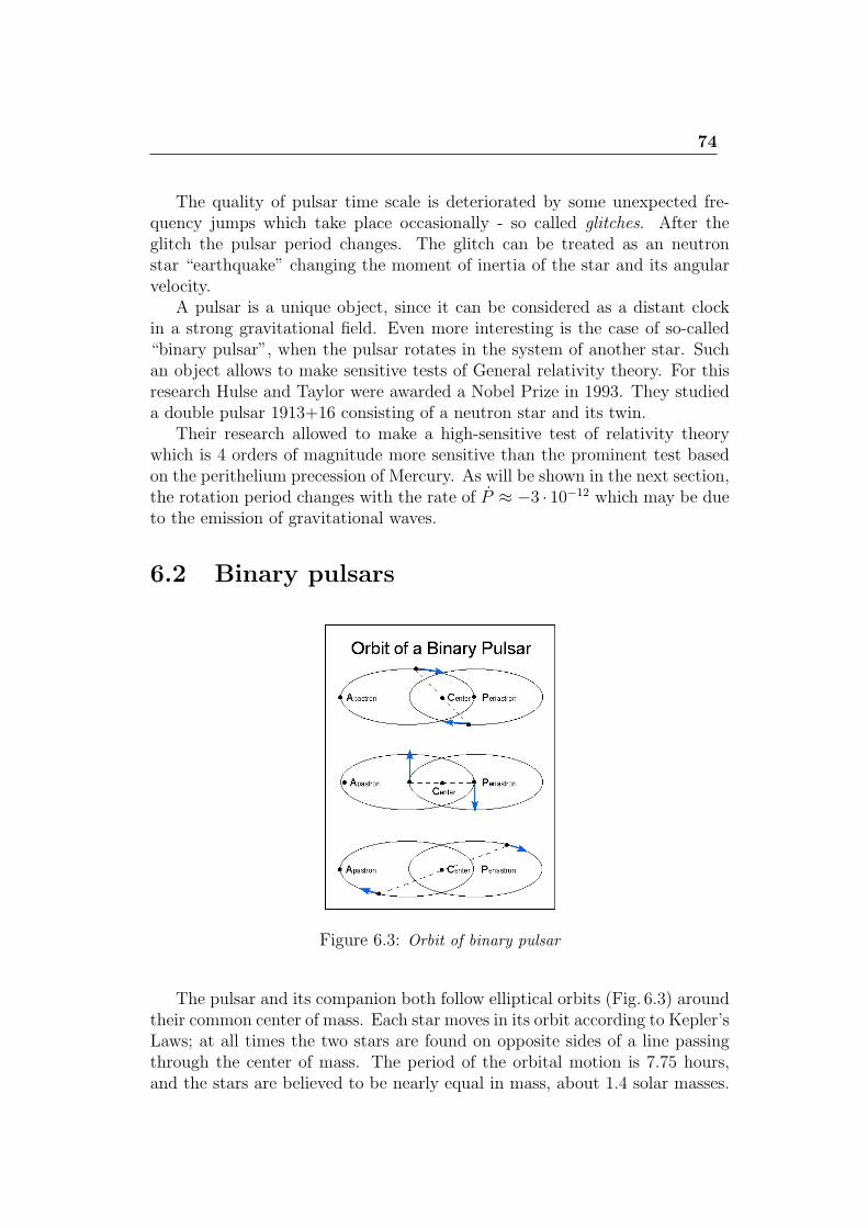
74

The quality of pulsar time scale is deteriorated by some unexpected fre-quency jumps which take place occasionally - so called glitches. After theglitch the pulsar period changes. The glitch can be treated as an neutronstar “earthquake” changing the moment of inertia of the star and its angularvelocity.

A pulsar is a unique object, since it can be considered as a distant clockin a strong gravitational field. Even more interesting is the case of so-called“binary pulsar”, when the pulsar rotates in the system of another star. Suchan object allows to make sensitive tests of General relativity theory. For thisresearch Hulse and Taylor were awarded a Nobel Prize in 1993. They studieda double pulsar 1913+16 consisting of a neutron star and its twin.

Their research allowed to make a high-sensitive test of relativity theorywhich is 4 orders of magnitude more sensitive than the prominent test basedon the perithelium precession of Mercury. As will be shown in the next section,the rotation period changes with the rate of P ≈ −3 · 10−12 which may be dueto the emission of gravitational waves.

6.2 Binary pulsars

Figure 6.3: Orbit of binary pulsar

The pulsar and its companion both follow elliptical orbits (Fig. 6.3) aroundtheir common center of mass. Each star moves in its orbit according to Kepler’sLaws; at all times the two stars are found on opposite sides of a line passingthrough the center of mass. The period of the orbital motion is 7.75 hours,and the stars are believed to be nearly equal in mass, about 1.4 solar masses.

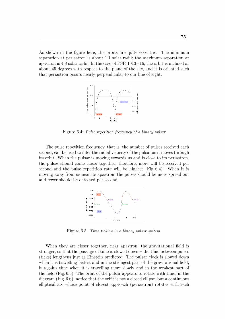
75

As shown in the figure here, the orbits are quite eccentric. The minimumseparation at periastron is about 1.1 solar radii; the maximum separation atapastron is 4.8 solar radii. In the case of PSR 1913+16, the orbit is inclined atabout 45 degrees with respect to the plane of the sky, and it is oriented suchthat periastron occurs nearly perpendicular to our line of sight.

Figure 6.4: Pulse repetition frequency of a binary pulsar

The pulse repetition frequency, that is, the number of pulses received eachsecond, can be used to infer the radial velocity of the pulsar as it moves throughits orbit. When the pulsar is moving towards us and is close to its periastron,the pulses should come closer together; therefore, more will be received persecond and the pulse repetition rate will be highest (Fig. 6.4). When it ismoving away from us near its apastron, the pulses should be more spread outand fewer should be detected per second.

Figure 6.5: Time ticking in a binary pulsar system.

When they are closer together, near apastron, the gravitational field isstronger, so that the passage of time is slowed down – the time between pulses(ticks) lengthens just as Einstein predicted. The pulsar clock is slowed downwhen it is travelling fastest and in the strongest part of the gravitational field;it regains time when it is travelling more slowly and in the weakest part ofthe field (Fig. 6.5). The orbit of the pulsar appears to rotate with time; in thediagram (Fig. 6.6), notice that the orbit is not a closed ellipse, but a continuouselliptical arc whose point of closest approach (periastron) rotates with each

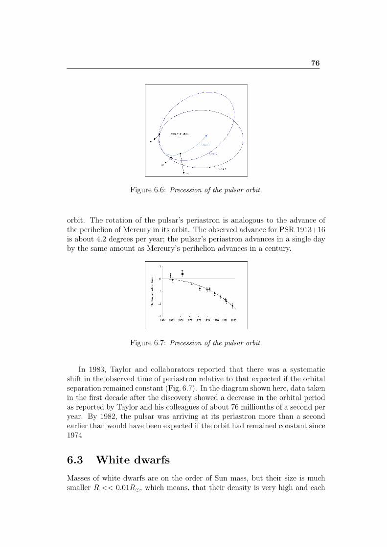
76

Figure 6.6: Precession of the pulsar orbit.

orbit. The rotation of the pulsar’s periastron is analogous to the advance ofthe perihelion of Mercury in its orbit. The observed advance for PSR 1913+16is about 4.2 degrees per year; the pulsar’s periastron advances in a single dayby the same amount as Mercury’s perihelion advances in a century.

Figure 6.7: Precession of the pulsar orbit.

In 1983, Taylor and collaborators reported that there was a systematicshift in the observed time of periastron relative to that expected if the orbitalseparation remained constant (Fig. 6.7). In the diagram shown here, data takenin the first decade after the discovery showed a decrease in the orbital periodas reported by Taylor and his colleagues of about 76 millionths of a second peryear. By 1982, the pulsar was arriving at its periastron more than a secondearlier than would have been expected if the orbit had remained constant since1974

6.3 White dwarfs

Masses of white dwarfs are on the order of Sun mass, but their size is muchsmaller R << 0.01R⊙, which means, that their density is very high and each

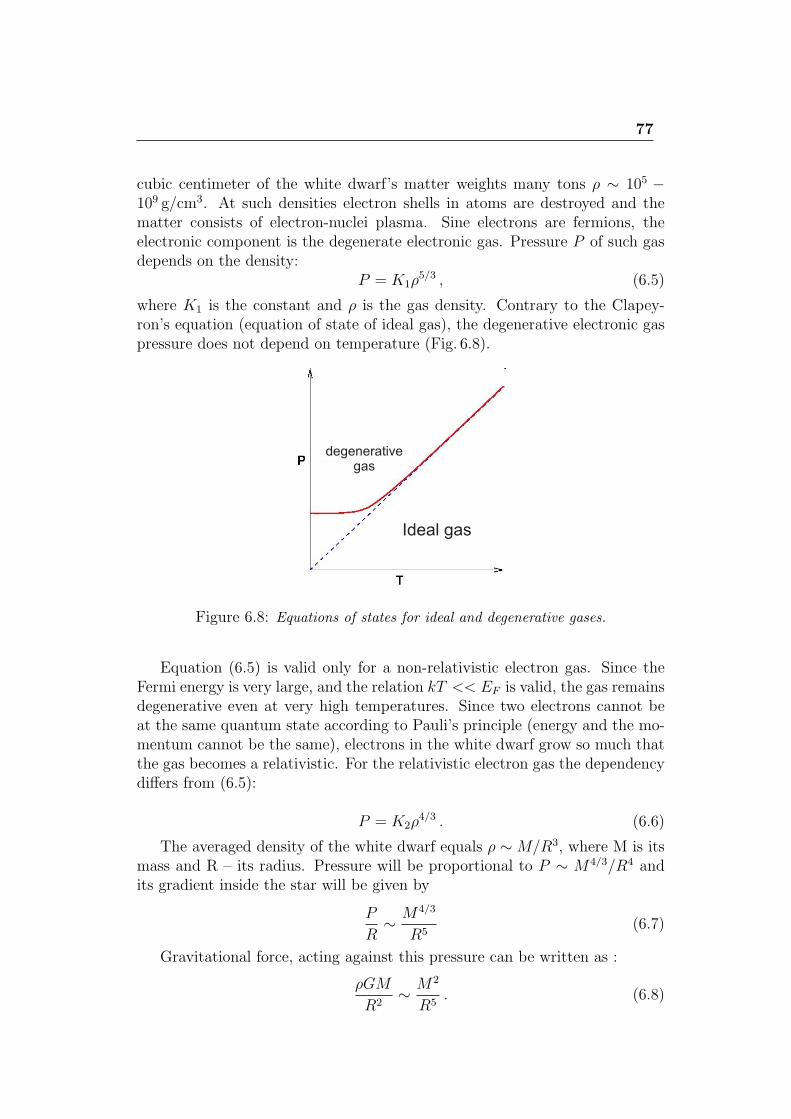
77

cubic centimeter of the white dwarf’s matter weights many tons ρ ∼ 105 −109 g/cm3. At such densities electron shells in atoms are destroyed and thematter consists of electron-nuclei plasma. Sine electrons are fermions, theelectronic component is the degenerate electronic gas. Pressure P of such gasdepends on the density:

P = K1ρ5/3 , (6.5)

where K1 is the constant and ρ is the gas density. Contrary to the Clapey-ron’s equation (equation of state of ideal gas), the degenerative electronic gaspressure does not depend on temperature (Fig. 6.8).

Figure 6.8: Equations of states for ideal and degenerative gases.

Equation (6.5) is valid only for a non-relativistic electron gas. Since theFermi energy is very large, and the relation kT << EF is valid, the gas remainsdegenerative even at very high temperatures. Since two electrons cannot beat the same quantum state according to Pauli’s principle (energy and the mo-mentum cannot be the same), electrons in the white dwarf grow so much thatthe gas becomes a relativistic. For the relativistic electron gas the dependencydiffers from (6.5):

P = K2ρ4/3 . (6.6)

The averaged density of the white dwarf equals ρ ∼M/R3, where M is itsmass and R – its radius. Pressure will be proportional to P ∼ M4/3/R4 andits gradient inside the star will be given by

P

R∼ M4/3

R5(6.7)

Gravitational force, acting against this pressure can be written as :

ρGM

R2∼ M2

R5. (6.8)

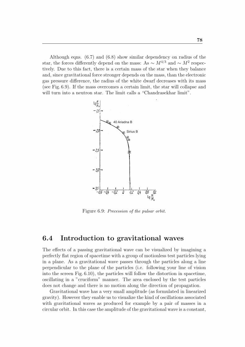
78

Although eqns. (6.7) and (6.8) show similar dependency on radius of thestar, the forces differently depend on the mass: As ∼M4/3 and ∼M2 respec-tively. Due to this fact, there is a certain mass of the star when they balanceand, since gravitational force stronger depends on the mass, than the electronicgas pressure difference, the radius of the white dwarf decreases with its mass(see Fig. 6.9). If the mass overcomes a certain limit, the star will collapse andwill turn into a neutron star. The limit calls a “Chandrasekhar limit”.

Figure 6.9: Precession of the pulsar orbit.

6.4 Introduction to gravitational waves

The effects of a passing gravitational wave can be visualized by imagining aperfectly flat region of spacetime with a group of motionless test particles lyingin a plane. As a gravitational wave passes through the particles along a lineperpendicular to the plane of the particles (i.e. following your line of visioninto the screen Fig. 6.10), the particles will follow the distortion in spacetime,oscillating in a ”cruciform” manner. The area enclosed by the test particlesdoes not change and there is no motion along the direction of propagation.

Gravitational wave has a very small amplitude (as formulated in linearizedgravity). However they enable us to visualize the kind of oscillations associatedwith gravitational waves as produced for example by a pair of masses in acircular orbit. In this case the amplitude of the gravitational wave is a constant,

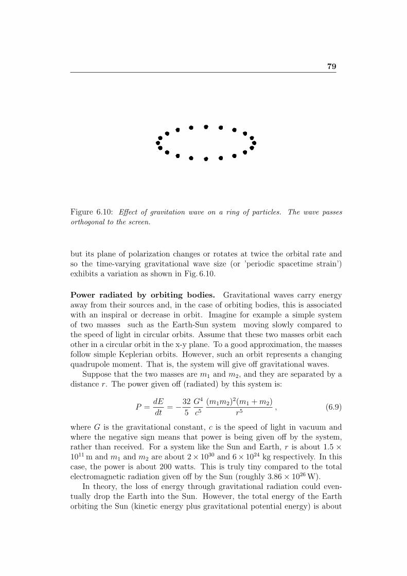
79

Figure 6.10: Effect of gravitation wave on a ring of particles. The wave passes

orthogonal to the screen.

but its plane of polarization changes or rotates at twice the orbital rate andso the time-varying gravitational wave size (or ’periodic spacetime strain’)exhibits a variation as shown in Fig. 6.10.

Power radiated by orbiting bodies. Gravitational waves carry energyaway from their sources and, in the case of orbiting bodies, this is associatedwith an inspiral or decrease in orbit. Imagine for example a simple systemof two masses such as the Earth-Sun system moving slowly compared tothe speed of light in circular orbits. Assume that these two masses orbit eachother in a circular orbit in the x-y plane. To a good approximation, the massesfollow simple Keplerian orbits. However, such an orbit represents a changingquadrupole moment. That is, the system will give off gravitational waves.

Suppose that the two masses are m1 and m2, and they are separated by adistance r. The power given off (radiated) by this system is:

P =dE

dt= −32

5

G4

c5(m1m2)

2(m1 +m2)

r5, (6.9)

where G is the gravitational constant, c is the speed of light in vacuum andwhere the negative sign means that power is being given off by the system,rather than received. For a system like the Sun and Earth, r is about 1.5 ×1011m and m1 and m2 are about 2× 1030 and 6× 1024 kg respectively. In thiscase, the power is about 200 watts. This is truly tiny compared to the totalelectromagnetic radiation given off by the Sun (roughly 3.86× 1026W).

In theory, the loss of energy through gravitational radiation could even-tually drop the Earth into the Sun. However, the total energy of the Earthorbiting the Sun (kinetic energy plus gravitational potential energy) is about

80

1.14 × 1036 joules of which only 200 joules per second is lost through gravi-tational radiation, leading to a decay in the orbit by about 10−15 meters perday or roughly the diameter of a proton. At this rate, it would take the Earthapproximately 1 × 1013 times more than the current age of the Universe tospiral onto the Sun.

Wave amplitudes from the EarthSun system. We can also think interms of the amplitude of the wave from a system in circular orbits. Let θbe the angle between the perpendicular to the plane of the orbit and the lineof sight of the observer. Suppose that an observer is outside the system at adistance R from its center of mass. If R is much greater than a wavelength,the two polarizations of the wave will be

h+ = − 1

R

G2

c42m1m2

r(1 + cos2 θ) cos [2ω(t−R)] (6.10)

h× = − 1

R

G2

c44m1m2

r(cos θ) sin [2ω(t−R)] . (6.11)

Here, we use the constant angular velocity of a circular orbit in Newtonianphysics: ω =

√G(m1 +m2)/r3.

For example, if the observer is in the x-y plane then θ = π/2, and cos(θ) =0, so the h× polarization is always zero. We also see that the frequency of thewave given off is twice the rotation frequency. If we put in numbers for theEarth-Sun system, we find:

h+ = − 1

R

G2

c44m1m2

r= − 1

R1.7× 10−10 meters. (6.12)

In this case, the minimum distance to find waves is R > 1 light-year, sotypical amplitudes will be h ∼ 10−26. That is, a ring of particles would stretchor squeeze by just one part in 1026. This is well under the detectability limitof all conceivable detectors.

6.4.1 Very Large Baseline Interferometry

Radio-astronomy played an important role in the study of astrophysical objectsproviding an essential information about our Universe. The smallest anglebetween two objects θ resolvable by a telescope equals to

θ = αλ

b. (6.13)

Diffraction on the aperture b limits he resolution of a telescope. The constantα is on the order of 1 and depends on the telescope’s shape and its illumination.

To reach resolution demanded by today’s goals, the size of radio-telescope(radio-telescopes typically work in the range from 1 cm to 1m) should be sobig that it cannot be implemented on practice.

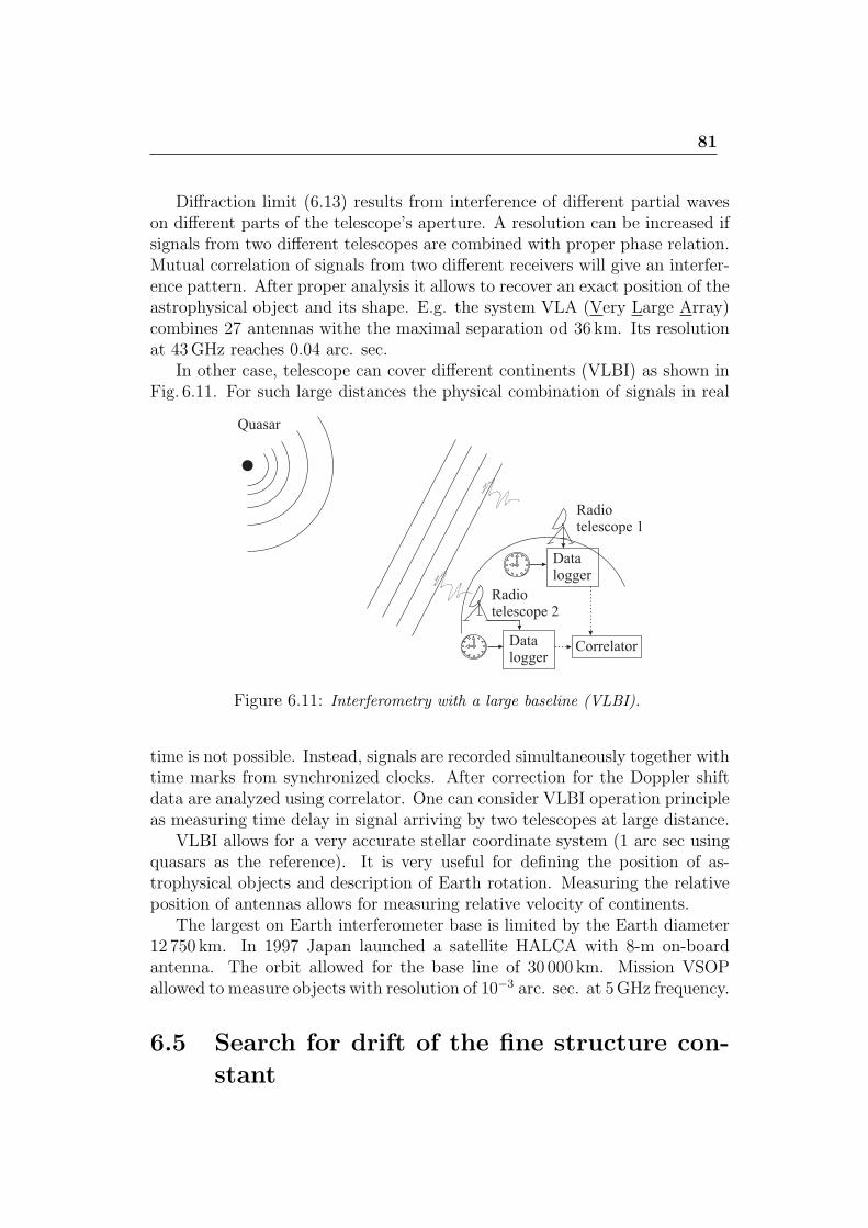
81

Diffraction limit (6.13) results from interference of different partial waveson different parts of the telescope’s aperture. A resolution can be increased ifsignals from two different telescopes are combined with proper phase relation.Mutual correlation of signals from two different receivers will give an interfer-ence pattern. After proper analysis it allows to recover an exact position of theastrophysical object and its shape. E.g. the system VLA (Very Large Array)combines 27 antennas withe the maximal separation od 36 km. Its resolutionat 43GHz reaches 0.04 arc. sec.

In other case, telescope can cover different continents (VLBI) as shown inFig. 6.11. For such large distances the physical combination of signals in real

Figure 6.11: Interferometry with a large baseline (VLBI).

time is not possible. Instead, signals are recorded simultaneously together withtime marks from synchronized clocks. After correction for the Doppler shiftdata are analyzed using correlator. One can consider VLBI operation principleas measuring time delay in signal arriving by two telescopes at large distance.

VLBI allows for a very accurate stellar coordinate system (1 arc sec usingquasars as the reference). It is very useful for defining the position of as-trophysical objects and description of Earth rotation. Measuring the relativeposition of antennas allows for measuring relative velocity of continents.

The largest on Earth interferometer base is limited by the Earth diameter12 750 km. In 1997 Japan launched a satellite HALCA with 8-m on-boardantenna. The orbit allowed for the base line of 30 000 km. Mission VSOPallowed to measure objects with resolution of 10−3 arc. sec. at 5GHz frequency.

6.5 Search for drift of the fine structure con-

stant

Lecture 7: Two levels atomicsystem and frequency standards

Optical Bloch equations. Pseudospin. Rabi oscillations. Excitation by sequenceof coherent pulses. Ramsey method. Atomic interferometry. Microwave fre-quency standards. Hydrogen maser. Cesium beam apparatus. Allan deviation,stability, accuracy.

7.1 Two-level system

Description of any atomic system is usually started from two-level model. Mostof the important processes like atomic level excitation, laser cooling, etc., areadequately described by this simplified model. Although most of the realatomic systems are very complex and have multiple levels, the two-level atom isstill a very important model which significantly helps understanding of physicalprocesses.

Consider a system with two levels with the energies E1 and E2, E2 > E1.The lower state is usually called the ground state and the upper state – excitedstate.

If two levels are coupled by an external field, the Hamiltonian can be writtenas

H = H0 +Hint . (7.1)

Here H0 presents the system itself, while interaction is given by Hint. For theHamiltonian H0 one can write the time-independent Schrodinger equation

H0ϕk(r) = Ekϕk(r) , (7.2)

without taking into account the spontaneous emission. Here k = 1, 2, and rdescribes all internal degrees of freedom (electron positions, spins). Externalfield cases perturbation Hint. Since eigenfunctions ϕk(r) form a full set , thegeneral solution ψ(r, t) of (7.8) can be given by their linear combination:

ψ(r, t) = c1(t)e−iE1t/hϕ1(r) + c2(t)e

−iE2t/hϕ2(r) . (7.3)

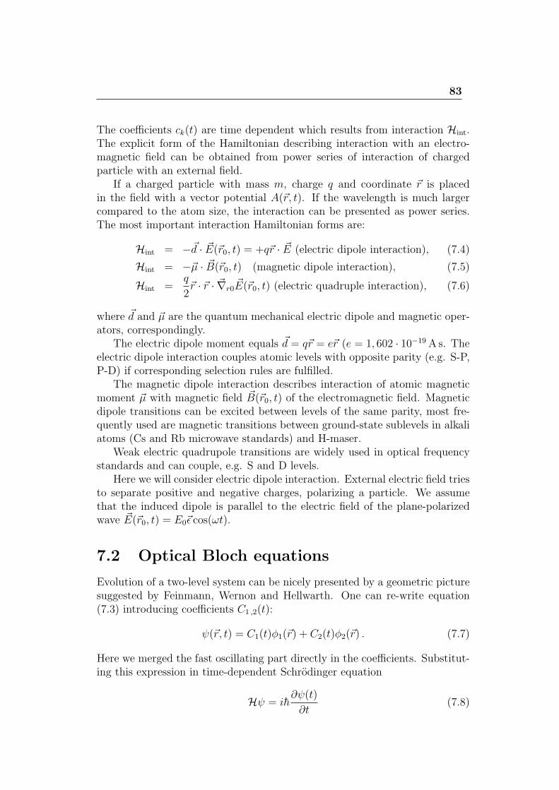
83

The coefficients ck(t) are time dependent which results from interaction Hint.The explicit form of the Hamiltonian describing interaction with an electro-magnetic field can be obtained from power series of interaction of chargedparticle with an external field.

If a charged particle with mass m, charge q and coordinate r is placedin the field with a vector potential A(r, t). If the wavelength is much largercompared to the atom size, the interaction can be presented as power series.The most important interaction Hamiltonian forms are:

Hint = −d · E(r0, t) = +qr · E (electric dipole interaction), (7.4)

Hint = −µ · B(r0, t) (magnetic dipole interaction), (7.5)

Hint =q

2r · r · ∇r0E(r0, t) (electric quadruple interaction), (7.6)

where d and µ are the quantum mechanical electric dipole and magnetic oper-ators, correspondingly.

The electric dipole moment equals d = qr = er (e = 1, 602 · 10−19 As. Theelectric dipole interaction couples atomic levels with opposite parity (e.g. S-P,P-D) if corresponding selection rules are fulfilled.

The magnetic dipole interaction describes interaction of atomic magneticmoment µ with magnetic field B(r0, t) of the electromagnetic field. Magneticdipole transitions can be excited between levels of the same parity, most fre-quently used are magnetic transitions between ground-state sublevels in alkaliatoms (Cs and Rb microwave standards) and H-maser.

Weak electric quadrupole transitions are widely used in optical frequencystandards and can couple, e.g. S and D levels.

Here we will consider electric dipole interaction. External electric field triesto separate positive and negative charges, polarizing a particle. We assumethat the induced dipole is parallel to the electric field of the plane-polarizedwave E(r0, t) = E0ϵ cos(ωt).

7.2 Optical Bloch equations

Evolution of a two-level system can be nicely presented by a geometric picturesuggested by Feinmann, Wernon and Hellwarth. One can re-write equation(7.3) introducing coefficients C1 ,2(t):

ψ(r, t) = C1(t)ϕ1(r) + C2(t)ϕ2(r) . (7.7)

Here we merged the fast oscillating part directly in the coefficients. Substitut-ing this expression in time-dependent Schrodinger equation

Hψ = ih∂ψ(t)

∂t(7.8)

84

Figure 7.1: A two-level system.

will give is the following set of equations:

dC1(t)

dt= +i

ω0

2C1(t)−

i

hC2(t)H12(t) (7.9)

dC2(t)

dt= −iω0

2C2(t)−

i

hC1(t)H21(t) . (7.10)

Here H21 ≡∫ϕ∗2Hintϕ1d

3r, H12 ≡∫ϕ∗1Hintϕ2d

3r = H∗21 and hω0 = E2 − E1.

The zero energy is taken as (E1 + E2)/2 = 0, which will give us E2 = hω0/2and E2 = −hω0/2. The sketch is shown in Fig. 7.1.

Feinmann used three real functions using coefficients C1(t) and C2(t):

R′1(t) ≡ C2(t)C

∗1(t) + C∗

2(t)C1(t) (7.11)

R′2(t) ≡ i[C2(t)C

∗1(t)− C∗

2(t)C1(t)] (7.12)

R′3(t) ≡ C2(t)C

∗2(t)− C1(t)C

∗1(t) , (7.13)

which and form a vector in the 3D space: R′(t) = (R′1(t), R

′2(t), R

′3(t)). This

vector is usually formally treated as a pseudospin vector. From (7.11) – (7.13)one can get a relation (the total population of the system equals 1)

R′12(t)+R′

22(t)+R′

32(t) = [C2(t)C

∗2(t)+C1(t)C

∗1(t)]

2 =(|c2(t)|2 + |c1(t)|2

)2= 1 .

(7.14)

The pseudospin length is constant and equals 1: |R′(t)|2 = 1. Its end movesalong some trajectory on so-called Bloch sphere of unit radius.

To understand the pseudospin components we will write equations describ-ing its evolution. For example, the derivative dR′

1(t)/dt can be calculated form(7.11):

dR′1(t)

dt=dC2(t)

dtC∗

1(t) + C2(t)dC∗

1(t)

dt+dC∗

2(t)

dtC1(t) + C∗

2(t)dC1(t)

dt. (7.15)

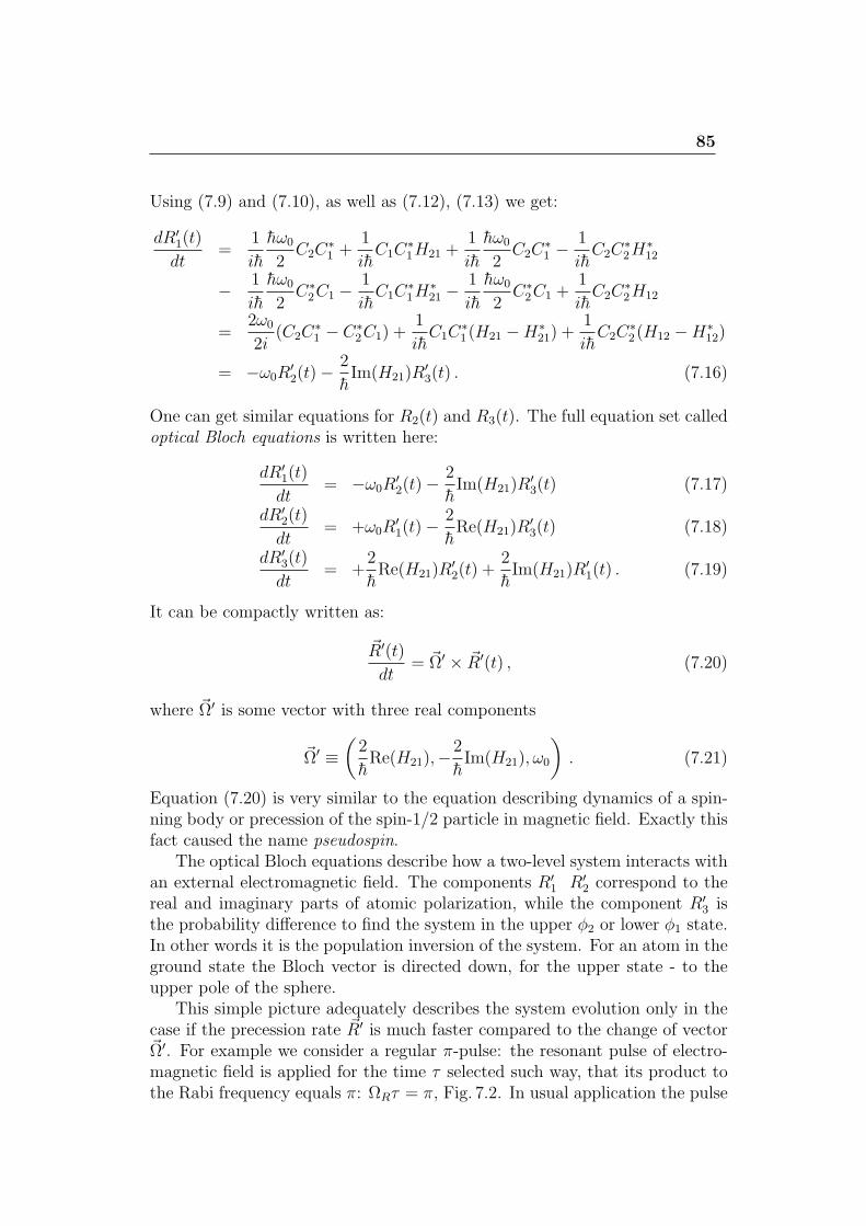
85

Using (7.9) and (7.10), as well as (7.12), (7.13) we get:

dR′1(t)

dt=

1

ih

hω0

2C2C

∗1 +

1

ihC1C

∗1H21 +

1

ih

hω0

2C2C

∗1 −

1

ihC2C

∗2H

∗12

− 1

ih

hω0

2C∗

2C1 −1

ihC1C

∗1H

∗21 −

1

ih

hω0

2C∗

2C1 +1

ihC2C

∗2H12

=2ω0

2i(C2C

∗1 − C∗

2C1) +1

ihC1C

∗1(H21 −H∗

21) +1

ihC2C

∗2(H12 −H∗

12)

= −ω0R′2(t)−

2

hIm(H21)R

′3(t) . (7.16)

One can get similar equations for R2(t) and R3(t). The full equation set calledoptical Bloch equations is written here:

dR′1(t)

dt= −ω0R

′2(t)−

2

hIm(H21)R

′3(t) (7.17)

dR′2(t)

dt= +ω0R

′1(t)−

2

hRe(H21)R

′3(t) (7.18)

dR′3(t)

dt= +

2

hRe(H21)R

′2(t) +

2

hIm(H21)R

′1(t) . (7.19)

It can be compactly written as:

R′(t)

dt= Ω′ × R′(t) , (7.20)

where Ω′ is some vector with three real components

Ω′ ≡(2

hRe(H21),−

2

hIm(H21), ω0

). (7.21)

Equation (7.20) is very similar to the equation describing dynamics of a spin-ning body or precession of the spin-1/2 particle in magnetic field. Exactly thisfact caused the name pseudospin.

The optical Bloch equations describe how a two-level system interacts withan external electromagnetic field. The components R′

1 R′2 correspond to the

real and imaginary parts of atomic polarization, while the component R′3 is

the probability difference to find the system in the upper ϕ2 or lower ϕ1 state.In other words it is the population inversion of the system. For an atom in theground state the Bloch vector is directed down, for the upper state - to theupper pole of the sphere.

This simple picture adequately describes the system evolution only in thecase if the precession rate R′ is much faster compared to the change of vectorΩ′. For example we consider a regular π-pulse: the resonant pulse of electro-magnetic field is applied for the time τ selected such way, that its product tothe Rabi frequency equals π: ΩRτ = π, Fig. 7.2. In usual application the pulse

86

Figure 7.2: The pseudospin vector is precessing around vector Ω′.

duration is much larger compared to the period of electromagnetic field andpseudospin rotates many time around the vertical axis of the Bloch sphere.

To get rid of these not informative multiple rotations, the pseudospin vectoris usually treated in the rotating frame u, v, w. It rotates with the frequencyof electromagnetic field ω around axis 3, the axis w coincides with axis 3.

We also assume, that interaction is electric dipole interaction and H12 =H∗

21 = −d · E (7.4). In this case the equations (7.17) – (7.19) can be re-writtenas:

dR′1(t)

dt= −ω0R

′2(t) (7.22)

dR′2(t)

dt= +ω0R

′1(t) +

2drhE0 cosωtR

′3(t) (7.23)

dR′3(t)

dt= −2dr

hE0 cosωtR

′2(t) . (7.24)

Now we can make the coordinate transformation according to

R′1(t) = u cosωt− v sinωt (7.25)

R′2(t) = u sinωt+ v cosωt (7.26)

R′3(t) = w . (7.27)

Substitution of (7.26) into (7.22) and replacing the derivative from (7.25) willgive us

u cosωt− v sinωt = (ω − ω0)u sinωt+ (ω − ω0)v cosωt (7.28)

u sinωt+ v cosωt = −(ω − ω0)u cosωt+ (ω − ω0)v sinωt+2drhE0 cosωtw

w = −2drhE0 cosωt sinωt u−

2drhE0 cos

2 ωt v .

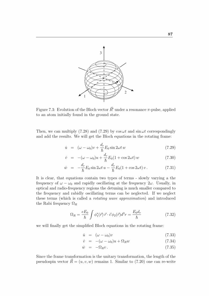
87

Figure 7.3: Evolution of the Bloch vector R′ under a resonance π-pulse, appliedto an atom initially found in the ground state.

Then, we can multiply (7.28) and (7.29) by cosωt and sinωt correspondinglyand add the results. We will get the Bloch equations in the rotating frame:

u = (ω − ω0)v +drhE0 sin 2ωtw (7.29)

v = −(ω − ω0)u+drhE0(1 + cos 2ωt)w (7.30)

w = −drhE0 sin 2ωt u−

drhE0(1 + cos 2ωt) v . (7.31)

It is clear, that equations contain two types of terms - slowly varying a thefrequency of ω − ω0 and rapidly oscillating at the frequency 2ω. Usually, inoptical and radio-frequency regions the detuning is much smaller compared tothe frequency and rabidly oscillating terms can be neglected. If we neglectthese terms (which is called a rotating wave approximation) and introducedthe Rabi frequency ΩR

ΩR =eE0

h

∫ϕ∗1(r) r · ϵ ϕ2(r)d

3r =E0drh

(7.32)

we will finally get the simplified Bloch equations in the rotating frame:

u = (ω − ω0)v (7.33)

v = −(ω − ω0)u+ ΩRw (7.34)

w = −ΩRv . (7.35)

Since the frame transformation is the unitary transformation, the length of thepseudospin vector R = (u, v, w) remains 1. Similar to (7.20) one can re-write

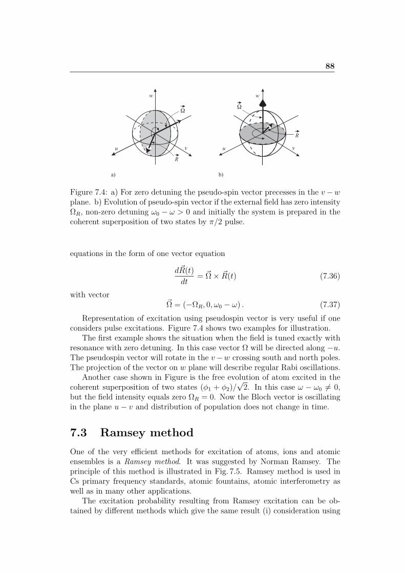
88

Figure 7.4: a) For zero detuning the pseudo-spin vector precesses in the v−wplane. b) Evolution of pseudo-spin vector if the external field has zero intensityΩR, non-zero detuning ω0 − ω > 0 and initially the system is prepared in thecoherent superposition of two states by π/2 pulse.

equations in the form of one vector equation

dR(t)

dt= Ω× R(t) (7.36)

with vectorΩ = (−ΩR, 0, ω0 − ω) . (7.37)

Representation of excitation using pseudospin vector is very useful if oneconsiders pulse excitations. Figure 7.4 shows two examples for illustration.

The first example shows the situation when the field is tuned exactly withresonance with zero detuning. In this case vector Ω will be directed along −u.The pseudospin vector will rotate in the v−w crossing south and north poles.The projection of the vector on w plane will describe regular Rabi oscillations.

Another case shown in Figure is the free evolution of atom excited in thecoherent superposition of two states (ϕ1 + ϕ2)/

√2. In this case ω − ω0 = 0,

but the field intensity equals zero ΩR = 0. Now the Bloch vector is oscillatingin the plane u− v and distribution of population does not change in time.

7.3 Ramsey method

One of the very efficient methods for excitation of atoms, ions and atomicensembles is a Ramsey method. It was suggested by Norman Ramsey. Theprinciple of this method is illustrated in Fig. 7.5. Ramsey method is used inCs primary frequency standards, atomic fountains, atomic interferometry aswell as in many other applications.

The excitation probability resulting from Ramsey excitation can be ob-tained by different methods which give the same result (i) consideration using

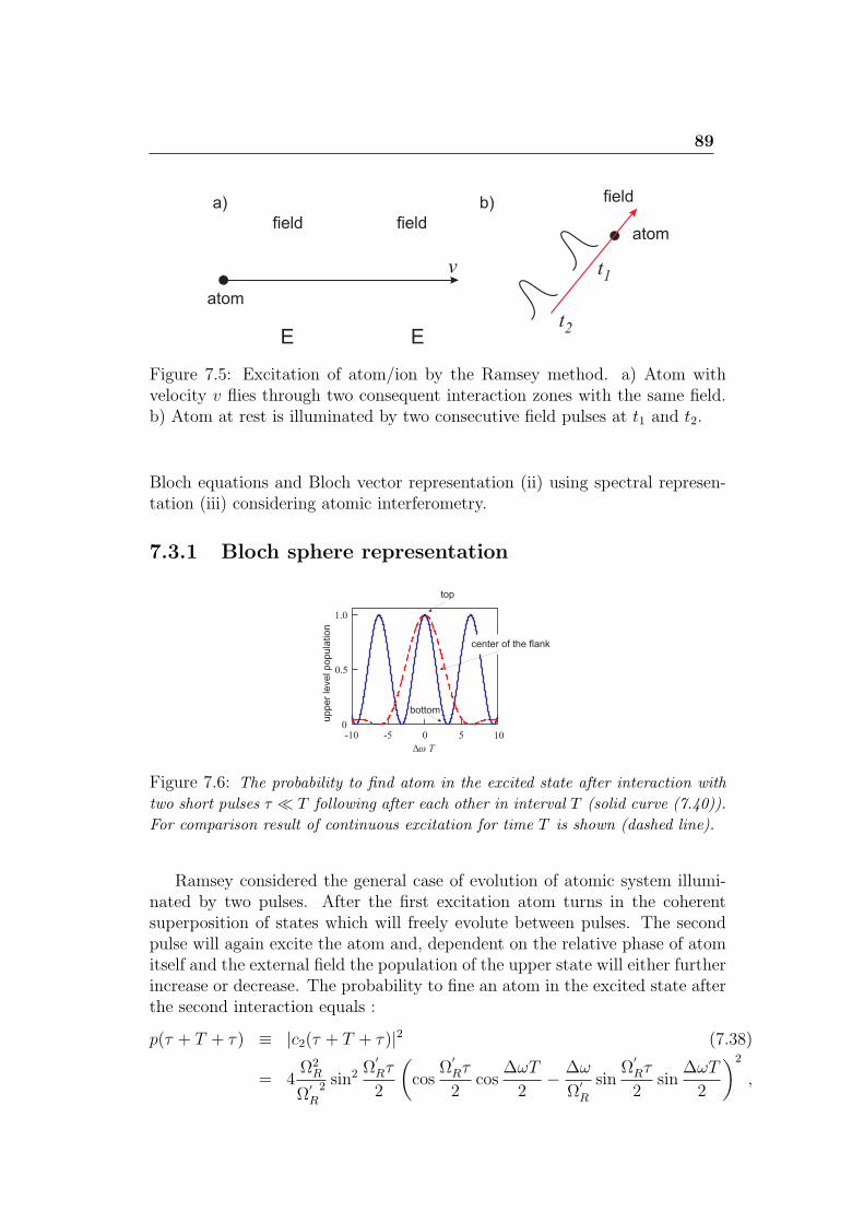
89

Figure 7.5: Excitation of atom/ion by the Ramsey method. a) Atom withvelocity v flies through two consequent interaction zones with the same field.b) Atom at rest is illuminated by two consecutive field pulses at t1 and t2.

Bloch equations and Bloch vector representation (ii) using spectral represen-tation (iii) considering atomic interferometry.

7.3.1 Bloch sphere representation

Figure 7.6: The probability to find atom in the excited state after interaction with

two short pulses τ ≪ T following after each other in interval T (solid curve (7.40)).

For comparison result of continuous excitation for time T is shown (dashed line).

Ramsey considered the general case of evolution of atomic system illumi-nated by two pulses. After the first excitation atom turns in the coherentsuperposition of states which will freely evolute between pulses. The secondpulse will again excite the atom and, dependent on the relative phase of atomitself and the external field the population of the upper state will either furtherincrease or decrease. The probability to fine an atom in the excited state afterthe second interaction equals :

p(τ + T + τ) ≡ |c2(τ + T + τ)|2 (7.38)

= 4Ω2

R

Ω′R2 sin

2 Ω′Rτ

2

(cos

Ω′Rτ

2cos

∆ωT

2− ∆ω

Ω′R

sinΩ

′Rτ

2sin

∆ωT

2

)2

,

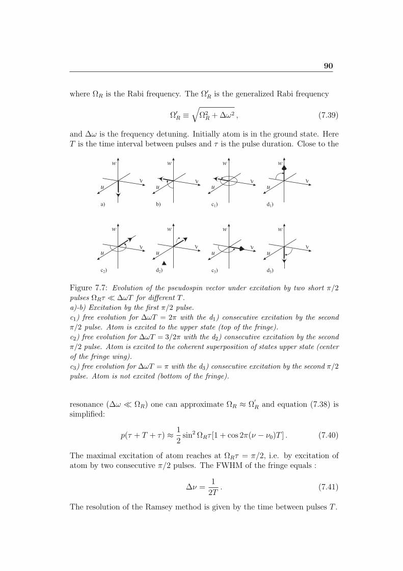
90

where ΩR is the Rabi frequency. The Ω′R is the generalized Rabi frequency

Ω′R ≡

√Ω2

R +∆ω2 , (7.39)

and ∆ω is the frequency detuning. Initially atom is in the ground state. HereT is the time interval between pulses and τ is the pulse duration. Close to the

Figure 7.7: Evolution of the pseudospin vector under excitation by two short π/2

pulses ΩRτ ≪ ∆ωT for different T .

a)-b) Excitation by the first π/2 pulse.

c1) free evolution for ∆ωT = 2π with the d1) consecutive excitation by the second

π/2 pulse. Atom is excited to the upper state (top of the fringe).

c2) free evolution for ∆ωT = 3/2π with the d2) consecutive excitation by the second

π/2 pulse. Atom is excited to the coherent superposition of states upper state (center

of the fringe wing).

c3) free evolution for ∆ωT = π with the d3) consecutive excitation by the second π/2

pulse. Atom is not excited (bottom of the fringe).

resonance (∆ω ≪ ΩR) one can approximate ΩR ≈ Ω′R and equation (7.38) is

simplified:

p(τ + T + τ) ≈ 1

2sin2 ΩRτ [1 + cos 2π(ν − ν0)T ] . (7.40)

The maximal excitation of atom reaches at ΩRτ = π/2, i.e. by excitation ofatom by two consecutive π/2 pulses. The FWHM of the fringe equals :

∆ν =1

2T. (7.41)

The resolution of the Ramsey method is given by the time between pulses T .

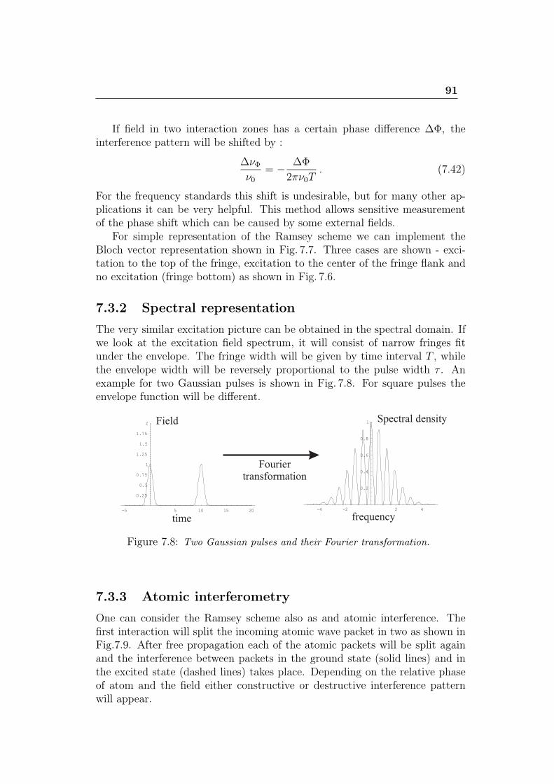
91

If field in two interaction zones has a certain phase difference ∆Φ, theinterference pattern will be shifted by :

∆νΦν0

= − ∆Φ

2πν0T. (7.42)

For the frequency standards this shift is undesirable, but for many other ap-plications it can be very helpful. This method allows sensitive measurementof the phase shift which can be caused by some external fields.

For simple representation of the Ramsey scheme we can implement theBloch vector representation shown in Fig. 7.7. Three cases are shown - exci-tation to the top of the fringe, excitation to the center of the fringe flank andno excitation (fringe bottom) as shown in Fig. 7.6.

7.3.2 Spectral representation

The very similar excitation picture can be obtained in the spectral domain. Ifwe look at the excitation field spectrum, it will consist of narrow fringes fitunder the envelope. The fringe width will be given by time interval T , whilethe envelope width will be reversely proportional to the pulse width τ . Anexample for two Gaussian pulses is shown in Fig. 7.8. For square pulses theenvelope function will be different.

Figure 7.8: Two Gaussian pulses and their Fourier transformation.

7.3.3 Atomic interferometry

One can consider the Ramsey scheme also as and atomic interference. Thefirst interaction will split the incoming atomic wave packet in two as shown inFig.7.9. After free propagation each of the atomic packets will be split againand the interference between packets in the ground state (solid lines) and inthe excited state (dashed lines) takes place. Depending on the relative phaseof atom and the field either constructive or destructive interference patternwill appear.

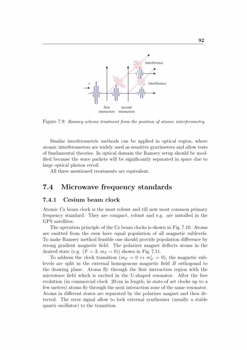
92

Figure 7.9: Ramsey scheme treatment from the position of atomic interferometry.

Similar interferometric methods can be applied in optical region, whereatomic interferometers are widely used as sensitive gravimeters and allow testsof fundamental theories. In optical domain the Ramsey setup should be mod-ified because the wave packets will be significantly separated in space due tolarge optical photon recoil.

All three mentioned treatments are equivalent.

7.4 Microwave frequency standards

7.4.1 Cesium beam clock

Atomic Cs beam clock is the most robust and till now most common primaryfrequency standard. They are compact, robust and e.g. are installed in theGPS satellites.

The operation principle of the Cs beam clocks is shown in Fig. 7.10. Atomsare emitted from the oven have equal population of all magnetic sublevels.To make Ramsey method feasible one should provide population difference bystrong gradient magnetic field. The polarizer magnet deflects atoms in thedesired state (e.g. (F = 3, mF = 0)) shown in Fig. 7.11.

To address the clock transition (mF = 0 ↔ m′F = 0), the magnetic sub-

levels are split in the external homogenous magnetic field B orthogonal tothe drawing plane. Atoms fly through the first interaction region with themicrowave field which is excited in the U-shaped resonator. After the freeevolution (in commercial clock 20 cm in length, in state-of art clocks up to afew meters) atoms fly through the next interaction zone of the same resonator.Atoms in different states are separated by the polarizer magnet and then de-tected. The error signal allow to lock external synthesizer (usually a stablequartz oscillator) to the transition.

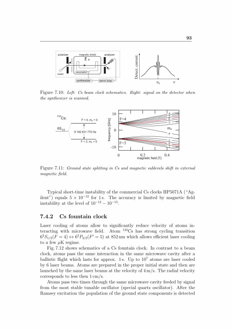
93

Figure 7.10: Left: Cs beam clock schematics. Right: signal on the detector when

the synthesizer is scanned.

Figure 7.11: Ground state splitting in Cs and magnetic sublevels shift in external

magnetic field.

Typical short-time instability of the commercial Cs clocks HP5071A (“Ag-ilent”) equals 5 × 10−12 for 1 s. The accuracy is limited by magnetic fieldinstability at the level of 10−12 − 10−13.

7.4.2 Cs fountain clock

Laser cooling of atoms allow to significantly reduce velocity of atoms in-teracting with microwave field. Atom 133Cs has strong cycling transition62S1/2(F = 4) ↔ 62P3/2(F

′ = 5) at 852 nm which allows efficient laser coolingto a few µK regime.

Fig. 7.12 shows schematics of a Cs fountain clock. In contrast to a beamclock, atoms pass the same interaction in the same microwave cavity after aballistic flight which lasts for approx. 1 s. Up to 107 atoms are laser cooledby 6 laser beams. Atoms are prepared in the proper initial state and then arelaunched by the same laser beams at the velocity of 4m/s. The radial velocitycorresponds to less then 1 cm/s.

Atoms pass two times through the same microwave cavity feeded by signalfrom the most stable tunable oscillator (special quartz oscillator). After theRamsey excitation the population of the ground state components is detected

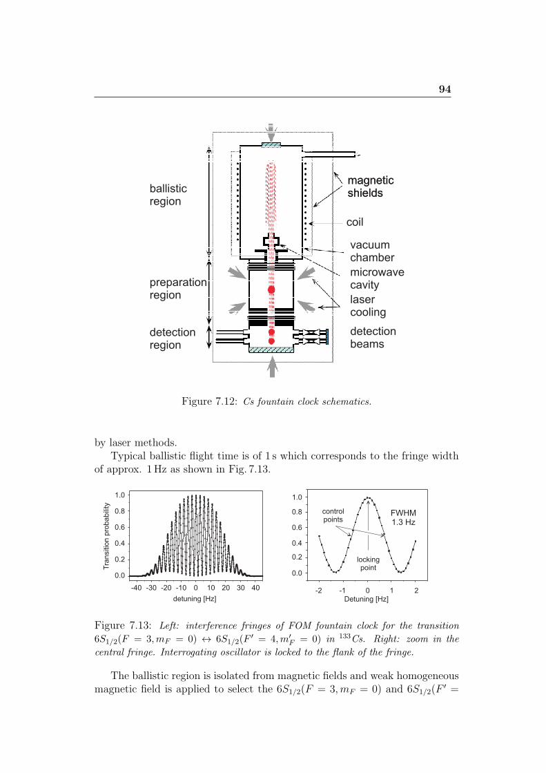
94

Figure 7.12: Cs fountain clock schematics.

by laser methods.Typical ballistic flight time is of 1 s which corresponds to the fringe width

of approx. 1Hz as shown in Fig. 7.13.

Figure 7.13: Left: interference fringes of FOM fountain clock for the transition

6S1/2(F = 3,mF = 0) ↔ 6S1/2(F′ = 4,m′

F = 0) in 133Cs. Right: zoom in the

central fringe. Interrogating oscillator is locked to the flank of the fringe.

The ballistic region is isolated from magnetic fields and weak homogeneousmagnetic field is applied to select the 6S1/2(F = 3,mF = 0) and 6S1/2(F

′ =

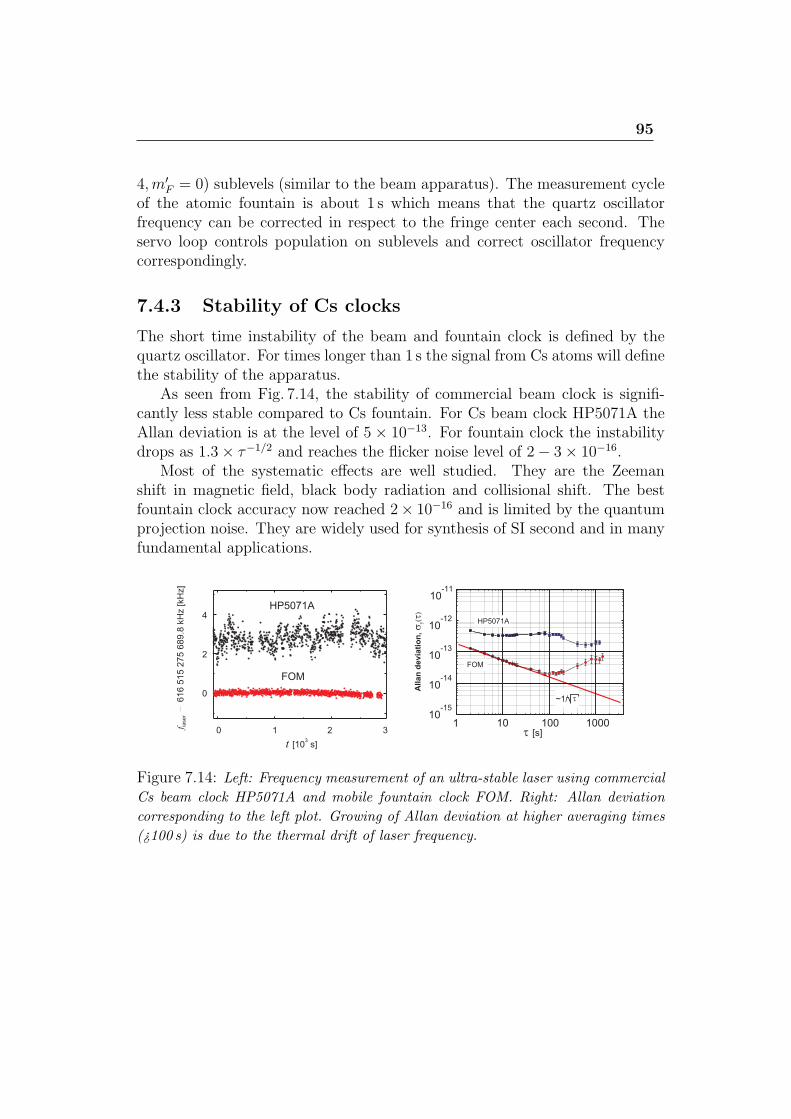
95

4,m′F = 0) sublevels (similar to the beam apparatus). The measurement cycle

of the atomic fountain is about 1 s which means that the quartz oscillatorfrequency can be corrected in respect to the fringe center each second. Theservo loop controls population on sublevels and correct oscillator frequencycorrespondingly.

7.4.3 Stability of Cs clocks

The short time instability of the beam and fountain clock is defined by thequartz oscillator. For times longer than 1 s the signal from Cs atoms will definethe stability of the apparatus.

As seen from Fig. 7.14, the stability of commercial beam clock is signifi-cantly less stable compared to Cs fountain. For Cs beam clock HP5071A theAllan deviation is at the level of 5× 10−13. For fountain clock the instabilitydrops as 1.3× τ−1/2 and reaches the flicker noise level of 2− 3× 10−16.

Most of the systematic effects are well studied. They are the Zeemanshift in magnetic field, black body radiation and collisional shift. The bestfountain clock accuracy now reached 2× 10−16 and is limited by the quantumprojection noise. They are widely used for synthesis of SI second and in manyfundamental applications.

Figure 7.14: Left: Frequency measurement of an ultra-stable laser using commercial

Cs beam clock HP5071A and mobile fountain clock FOM. Right: Allan deviation

corresponding to the left plot. Growing of Allan deviation at higher averaging times

(¿100 s) is due to the thermal drift of laser frequency.

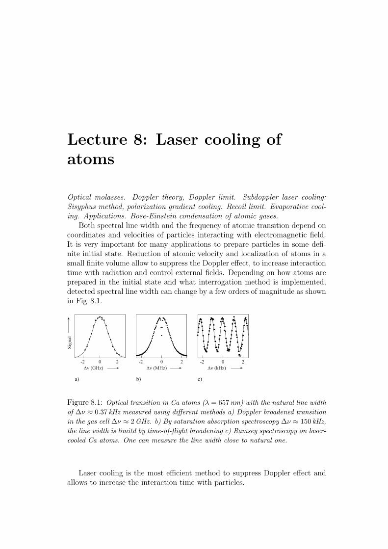
Lecture 8: Laser cooling ofatoms

Optical molasses. Doppler theory, Doppler limit. Subdoppler laser cooling:Sisyphus method, polarization gradient cooling. Recoil limit. Evaporative cool-ing. Applications. Bose-Einstein condensation of atomic gases.

Both spectral line width and the frequency of atomic transition depend oncoordinates and velocities of particles interacting with electromagnetic field.It is very important for many applications to prepare particles in some defi-nite initial state. Reduction of atomic velocity and localization of atoms in asmall finite volume allow to suppress the Doppler effect, to increase interactiontime with radiation and control external fields. Depending on how atoms areprepared in the initial state and what interrogation method is implemented,detected spectral line width can change by a few orders of magnitude as shownin Fig. 8.1.

Figure 8.1: Optical transition in Ca atoms (λ = 657 nm) with the natural line width

of ∆ν ≈ 0.37 kHz measured using different methods a) Doppler broadened transition

in the gas cell ∆ν ≈ 2GHz. b) By saturation absorption spectroscopy ∆ν ≈ 150 kHz,

the line width is limitd by time-of-flight broadening c) Ramsey spectroscopy on laser-

cooled Ca atoms. One can measure the line width close to natural one.

Laser cooling is the most efficient method to suppress Doppler effect andallows to increase the interaction time with particles.

97

Laser cooling of neutral atoms was first suggested by Hansch and Shawlow(1975), while Weinland and Demelt suggested laser cooling of ions (1975).

8.1 Optical molasses

Let us take a two-level atom with the ground and excited state energies ofEg and Ee correspondingly. It absorbs a photon from a laser field with the

wave vector k and the momentum of hk. After absorption it spontaneouslyemits a photon. Laser frequency is red detuned from the transition frequency(Ee − Eg)/h. The photon momentum is transferred to the atom changingatom’s momentum p = mv. Assume that the Doppler shift ∆ν = p/(mλ) issmall in respect to the natural line width γ = 1/(2πτ), where τ is the lifetime of the excited state. It means that ∆ν ≪ γ. Under this assumption thetransferred momentum ∆p = hk can be averaged out by a large number ofabsorption and emission processes which results in a classical force F appliedto an atom. Spontaneously emitted photons will not contribute to the forceF , because they are emitted isotropically. The averaged force applied to anatom from absorbed photons equals to :

F =Ne

N

hk

τ, (8.1)

where Ne is the averaged number of atoms in the excited state, and N =Ne +Ng is the total number of atoms (the sum of excited state atoms Ne andground state atoms Ng). The ratio Ne/N can be derived using the saturationparameter S0 which will give us :

F =hk

2τ

S0

1 + S0 +(

δνγ/2

)2 . (8.2)

Here

S0 ≡I

Isat, (8.3)

where Isat is the saturation intensity corresponding to the case when the res-onant radiation transfers 1/4 of the population to the excited level. It can bewritten as

Isat =2π2hcγ

3λ3. (8.4)

Theory of a two-level system describes the population of the upper level as

Ne

N=S0

2

(γ/2)2

(1 + S0)(γ/2)2 + δν2, (8.5)

which, after substitution, will give the result (8.2).

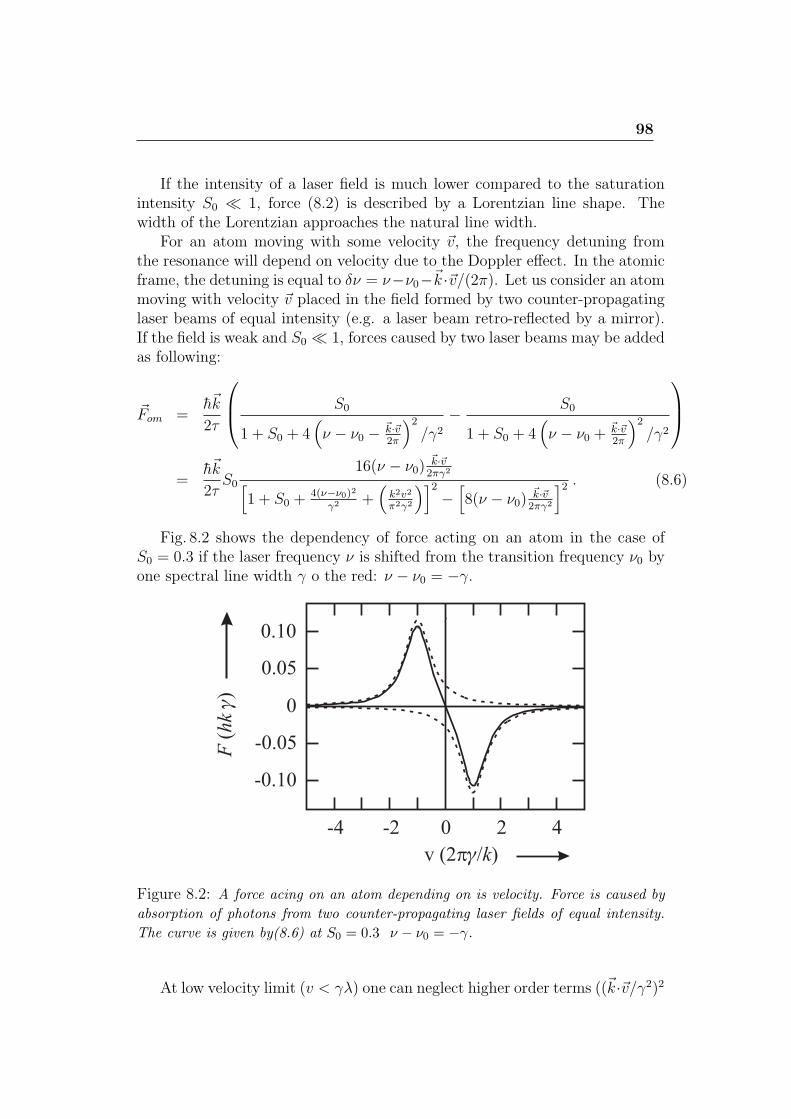
98

If the intensity of a laser field is much lower compared to the saturationintensity S0 ≪ 1, force (8.2) is described by a Lorentzian line shape. Thewidth of the Lorentzian approaches the natural line width.

For an atom moving with some velocity v, the frequency detuning fromthe resonance will depend on velocity due to the Doppler effect. In the atomicframe, the detuning is equal to δν = ν−ν0−k ·v/(2π). Let us consider an atommoving with velocity v placed in the field formed by two counter-propagatinglaser beams of equal intensity (e.g. a laser beam retro-reflected by a mirror).If the field is weak and S0 ≪ 1, forces caused by two laser beams may be addedas following:

Fom =hk

2τ

S0

1 + S0 + 4(ν − ν0 − k·v

2π

)2/γ2

− S0

1 + S0 + 4(ν − ν0 +

k·v2π

)2/γ2

=

hk

2τS0

16(ν − ν0)k·v2πγ2[

1 + S0 +4(ν−ν0)2

γ2 +(

k2v2

π2γ2

)]2−[8(ν − ν0)

k·v2πγ2

]2 . (8.6)

Fig. 8.2 shows the dependency of force acting on an atom in the case ofS0 = 0.3 if the laser frequency ν is shifted from the transition frequency ν0 byone spectral line width γ o the red: ν − ν0 = −γ.

Figure 8.2: A force acing on an atom depending on is velocity. Force is caused by

absorption of photons from two counter-propagating laser fields of equal intensity.

The curve is given by(8.6) at S0 = 0.3 ν − ν0 = −γ.

At low velocity limit (v < γλ) one can neglect higher order terms ((k·v/γ2)2

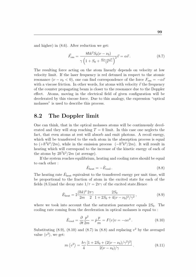
99

and higher) in (8.6). After reduction we get:

Fom =8hk2S0(ν − ν0)

γ(1 + S0 +

4(ν−ν0)2

γ2

)2 v = αv . (8.7)

The resulting force acting on the atom linearly depends on velocity at lowvelocity limit. If the laser frequency is red detuned in respect to the atomicresonance (ν − ν0 < 0), one can find correspondence of the force Fom = −αvwith a viscose friction. In other words, for atoms with velocity v the frequencyof the counter propagating beam is closer to the resonance due to the Dopplereffect. Atoms, moving in the electrical field of given configuration will bedecelerated by this viscose force. Due to this analogy, the expression “opticalmolasses” is used to describe this process.

8.2 The Doppler limit

One can think, that in the optical molasses atoms will be continuously decel-erated and they will stop reaching T = 0 limit. In this case one neglects thefact, that even atoms at rest will absorb and emit photons. A recoil energy,which will be transferred to the each atom in the absorption process is equalto (+h2k2/2m), while in the emission process (−h2k2/2m). It will result inheating which will correspond to the increase of the kinetic energy of each ofthe atoms by 2h2k2/2m (at average).

If the system reaches equilibrium, heating and cooling rates should be equalto each other :

Eheat = −Ecool . (8.8)

The heating rate Eheat equivalent to the transferred energy per unit time, willbe proportional to the fraction of atom in the excited state for each of thefields (8.5)and the decay rate 1/τ = 2πγ of the excited state.Hence

Eheat = 2(hk)2

2m

2πγ

2

2S0

1 + 2S0 + 4(ν − ν0)2/γ2, (8.9)

where we took into account that the saturation parameter equals 2S0. Thecooling rate coming from the deceleration in optical molasses is equal to :

Ecool =∂

∂t

p2

2m= p

p

m= F (v)v = −αv2 . (8.10)

Substituting (8.9), (8.10) and (8.7) in (8.8) and replacing v2 by the averagedvalue ⟨v2⟩, we get:

m⟨v2⟩=hγ

4

[1 + 2S0 + (2(ν − ν0)/γ2)2]

2(ν − ν0)/γ. (8.11)

100

The right part of the equation (8.11) reaches minimum at ν−ν0 = γ/2. Takinginto account that m ⟨v2⟩ /2 = kBT/2, we get, that the minimal temperatureequals to:

TD =hγ

2kB=

hΓ

2kB(Doppler limit) (8.12)

under condition S0 → 0. Temperature TD is the minimal temperature whichcan be achieved using considered cooling mechanism. Since the cooling resultsfrom the Doppler effect, the temperature limit is referred as to Doppler limit.

The Doppler limit in the three-dimensional case can be derived by similarconsiderations. Although the cooling rate is the same as in one-dimensionalcase, the heating rate will be three times higher, because in 3D case one shouldtake into account 6 laser field instead of two.At the other hand side, the tem-perature is given by m ⟨v2⟩3D /2 = 3kBT/2. As a result, the Doppler limitin the 3D case is the same, as in (8.12). E.g., for Cs atoms with the coolingtransition 6 2S1/2 – 6

2P3/2 (λ = 852 nm, γ = 5, 18MHz), the Doppler limitequals 0, 12mK. For Ca atoms and corresponding cooling transition 41S0 –41P1 (λ = 423 nm, γ = 34, 6 Hz) – 0, 83mK. Thermal velocity correspondingto Doppler limit can be obtained from the equation 1/2mv2D = kBTD/2 :

vD =

√hγ

2m. (8.13)

For the examples given above vD,Cs = 8, 82 cm/s vD,Ca = 41, 5 cm/s.

8.3 Subdoppler cooling

Typical velocities of atoms cooled using the Doppler mechanism on strongresonance transitions are in the range from a few cm/s to few tens cm/s.Although it is much less compared to the thermal velocity of atoms (typically300-500 m/s), they are still too high for many applications. For example, inthe atomic fountain clock atoms should interact with radiation within 1 s. Toload atoms in the shallow traps one also have to cool atoms to lower velocities.

For atoms possessing magnetic or hyperfine splitting of the ground state(e.g. Cs, Rb, Tm, etc.) there are other mechanisms which allow to laser coolatoms to even lower temperatures. Most frequency implemented is so called po-larization gradient method were atoms are cooled in a laser field with spatiallyvarying polarization. The gradient can be formed by two counter-propagatinglaser fields of opposite circular polarization or two counter-propagating laserfields of orthogonal linear polarizations which is called “Sisyphus cooling”. Wewill consider this mechanism as an example.

For Sisyphus laser cooling the atom should move in two laser fields of equalamplitudes and frequencies, opposite wave vectors and perpendicular linear

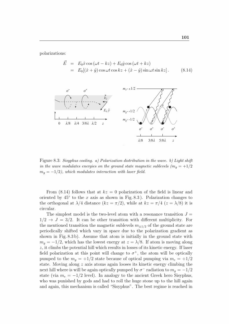
101

polarizations:

E = E0x cos (ωt− kz) + E0y cos (ωt+ kz)

= E0[(x+ y) cosωt cos kz + (x− y) sinωt sin kz] . (8.14)

Figure 8.3: Sisyphus cooling. a) Polarization distribution in the wave. b) Light shift

in the wave modulates energies on the ground state magnetic sublevels (mg = +1/2

mg = −1/2), which modulates interaction with laser field.

From (8.14) follows that at kz = 0 polarization of the field is linear andoriented by 45 to the x axis as shown in Fig. 8.3 ). Polarization changes tothe orthogonal at λ/4 distance (kz = π/2), while at kz = π/4 (z = λ/8) it iscircular.

The simplest model is the two-level atom with a resonance transition J =1/2 → J = 3/2. It can be other transition with different multiplicity. Forthe mentioned transition the magnetic sublevels m±1/2 of the ground state areperiodically shifted which vary in space due to the polarization gradient asshown in Fig. 8.3 b). Assume that atom is initially in the ground state withmg = −1/2, which has the lowest energy at z = λ/8. If atom is moving alongz, it climbs the potential hill which results in losses of its kinetic energy. If laserfield polarization at this point will change to σ+, the atom will be opticallypumped to the mg = +1/2 state because of optical pumping via me = +1/2state. Moving along z axis atoms again looses its kinetic energy climbing thenext hill where is will be again optically pumped by σ− radiation tomg = −1/2state (via me = −1/2 level). In analogy to the ancient Greek hero Sisyphus,who was punished by gods and had to roll the huge stone up to the hill againand again, this mechanism is called “Sisyphus”. The best regime is reached in

102

the case if the averaged time of optical pumping necessary to transfer atomsto the next sublevel equals the travelling time of λ/2 distance.

Usually, in the experiment the polarizations are chosen to be σ+/σ− andslightly different mechanism plays a role. In this case the resulting polarizationwill be always linear, but rotating around the axis. Cooling will be reached byperiodical re-distribution of population among the sublevels which will increaseprobability to absorb photon from the light field counter propagating to theatomic motion.

The minimal temperature which can be reached using subdoppler mecha-nism reaches the recoil limit

kBT > Er = (hk)2/2m. (8.15)

For Cs atoms in 3D optical molasses the achievable temperature is 25µK,which is much lower than the Doppler limit 0, 12mK, but still slightly highercompared to (8.15).

The recoil limit is difficult to overcome since it results from only one singleemission of a resonance photon. Still, there are approaches allowing to lasercool atoms to even lower temperatures (e.g. by using EIT and Raman cooling),but in this case atom should not directly interact with the resonance laserfield scattering photons. These exotic methods have not find applications infrequency standards.

One can reach low temperatures also by implementation of the second stageDoppler cooling, but using narrower transition. It is useful for atoms which donot have magnetic splitting of the ground state: 20Mg, 40Ca, 88Sr all of themwidely used in frequency standards. Using transitions of ∼ 1Hz line width onecan push the Doppler limit to microkelvin regime.

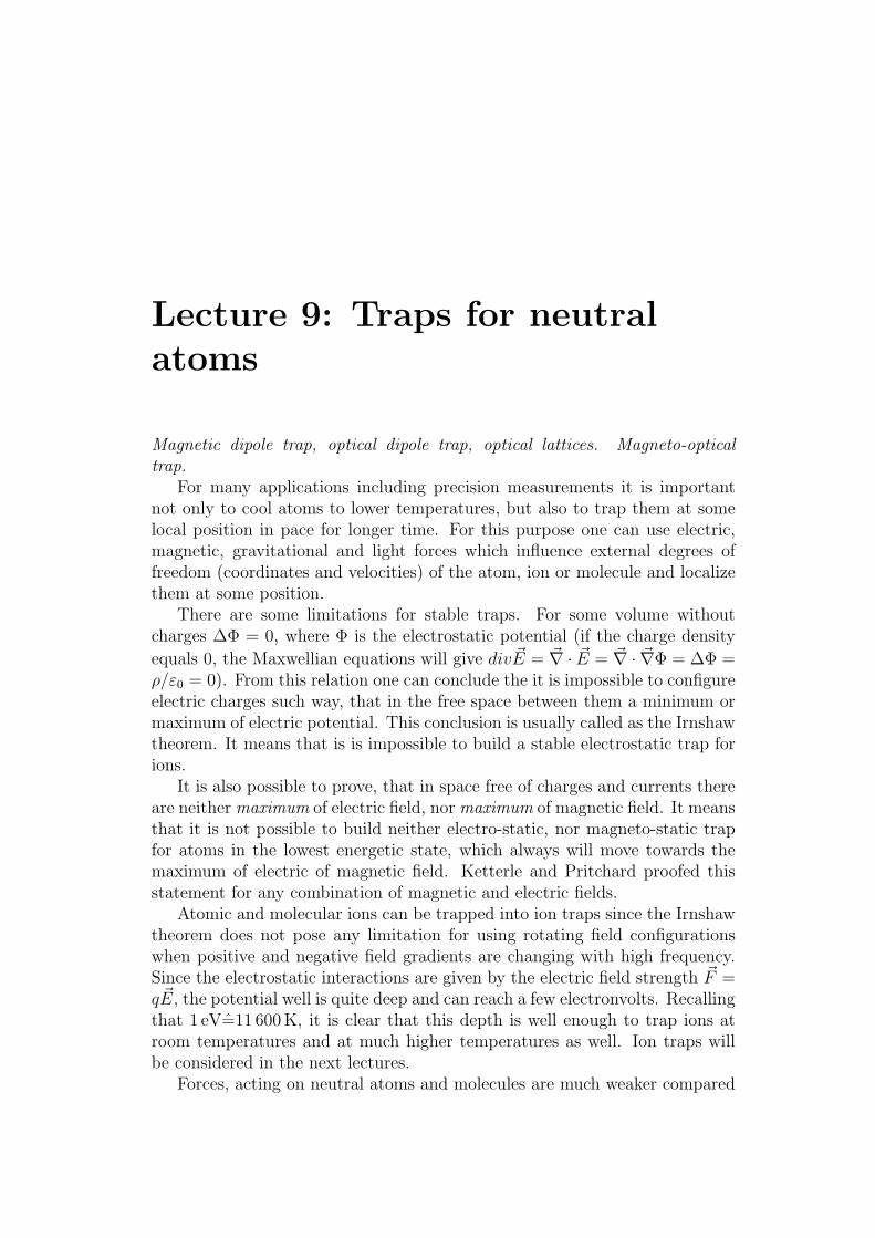
Lecture 9: Traps for neutralatoms

Magnetic dipole trap, optical dipole trap, optical lattices. Magneto-opticaltrap.

For many applications including precision measurements it is importantnot only to cool atoms to lower temperatures, but also to trap them at somelocal position in pace for longer time. For this purpose one can use electric,magnetic, gravitational and light forces which influence external degrees offreedom (coordinates and velocities) of the atom, ion or molecule and localizethem at some position.

There are some limitations for stable traps. For some volume withoutcharges ∆Φ = 0, where Φ is the electrostatic potential (if the charge density

equals 0, the Maxwellian equations will give divE = ∇ · E = ∇ · ∇Φ = ∆Φ =ρ/ε0 = 0). From this relation one can conclude the it is impossible to configureelectric charges such way, that in the free space between them a minimum ormaximum of electric potential. This conclusion is usually called as the Irnshawtheorem. It means that is is impossible to build a stable electrostatic trap forions.

It is also possible to prove, that in space free of charges and currents thereare neither maximum of electric field, nor maximum of magnetic field. It meansthat it is not possible to build neither electro-static, nor magneto-static trapfor atoms in the lowest energetic state, which always will move towards themaximum of electric of magnetic field. Ketterle and Pritchard proofed thisstatement for any combination of magnetic and electric fields.

Atomic and molecular ions can be trapped into ion traps since the Irnshawtheorem does not pose any limitation for using rotating field configurationswhen positive and negative field gradients are changing with high frequency.Since the electrostatic interactions are given by the electric field strength F =qE, the potential well is quite deep and can reach a few electronvolts. Recallingthat 1 eV=11 600K, it is clear that this depth is well enough to trap ions atroom temperatures and at much higher temperatures as well. Ion traps willbe considered in the next lectures.

Forces, acting on neutral atoms and molecules are much weaker compared

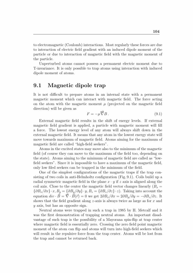
104

to electromagnetic (Coulomb) interactions. Most regularly these forces are dueto interaction of electric field gradient with an induced dipole moment of theparticle or due to interaction of magnetic field with the magnetic moment ofthe particle.

Unperturbed atoms cannot possess a permanent electric moment due toT-invariance. It is only possible to trap atoms using interaction with induceddipole moment of atoms.

9.1 Magnetic dipole trap

It is not difficult to prepare atoms in an internal state with a permanentmagnetic moment which can interact with magnetic field. The force actingon the atom with the magnetic moment µ (projected on the magnetic fielddirection) will be given as

F = −µ−→∇B . (9.1)

External magnetic field results in the shift of energy levels. If externalmagnetic field gradient is applied, a particle with magnetic moment will filla force. The lowest energy level of any atom will always shift down in theexternal magnetic field. It means that any atom in the lowest energy state willmove towards maximum of magnetic field. Atoms aiming for the maximum ofmagnetic field are called “high-field seekers”.

Atoms in the excited states may move also to the minimum of the magneticfield (of course they can move to the maximum of the field too, depending onthe state). Atoms aiming to the minimum of magnetic field are called as “low-field seekers”. Since it is impossible to have a maximum of the magnetic field,only low filed seekers can be trapped in the minimum of the field.

One of the simplest configurations of the magnetic traps if the trap con-sisting of two coils in anti-Helmholtz configuration (Fig. 9.1). Coils build up aradial symmetric magnetic field in the plane x – y if z axis is aligned along thecoil axis. Close to the center the magnetic field vector changes linearly (Bx =∂Bx/∂x ·x,By = ∂By/∂y ·y,Bz = ∂Bz/∂z · z). Taking into account the

equation div · B = ∇ · B(r) = 0 we get 2∂Bx/∂x = 2∂By/∂y = −∂Bz/∂z. Itshows that the field gradient along z-axis is always twice as large as for x andy axis, but has an opposite sign.

Neutral atoms were trapped in such a trap in 1985 by H. Metcalf and itwas the first demonstration of trapping neutral atoms. An important disad-vantage of such trap is the possibility of a Mayorana spin-flip at trap centerwhere magnetic field is essentially zero. Crossing the zero field point magneticmoment of the atom can flip and atoms will turn into high-field seekers whichwill result in the repulsive force from the trap center. Atoms will be lost fromthe trap and cannot be returned back.

105

Figure 9.1: Magnetic quadrupole trap consisting of two current loops in the anti-

Helmholtz configuration.

Figure 9.2: Ioffe-Pritchard trap consisting of four current lines and two coils. Ar-

rows show direction of current.

One of the possible solutions is the implementation of the Ioffe-Proitchardtrap shown in Fig. 9.2. Such trap possesses the minimum of the magnetic fieldas well, but the field does not turn to zero at its minimum. Such systems arewidely used for production of quantum degenerative gases (Bose-Einstein andFermi condensates).

Both these systems have very shallow potential gap and can be imple-mented only for trapping neutral particles at very low temperatures (less than1 K).

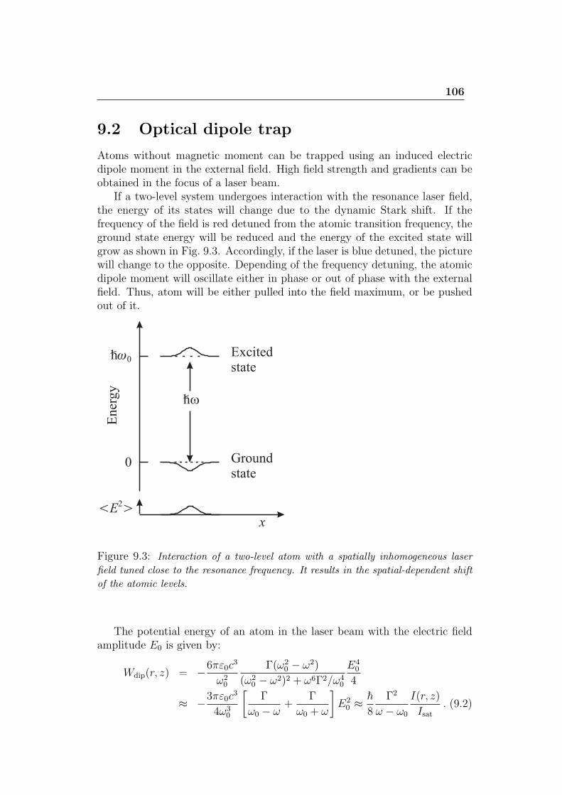
106

9.2 Optical dipole trap

Atoms without magnetic moment can be trapped using an induced electricdipole moment in the external field. High field strength and gradients can beobtained in the focus of a laser beam.

If a two-level system undergoes interaction with the resonance laser field,the energy of its states will change due to the dynamic Stark shift. If thefrequency of the field is red detuned from the atomic transition frequency, theground state energy will be reduced and the energy of the excited state willgrow as shown in Fig. 9.3. Accordingly, if the laser is blue detuned, the picturewill change to the opposite. Depending of the frequency detuning, the atomicdipole moment will oscillate either in phase or out of phase with the externalfield. Thus, atom will be either pulled into the field maximum, or be pushedout of it.

Figure 9.3: Interaction of a two-level atom with a spatially inhomogeneous laser

field tuned close to the resonance frequency. It results in the spatial-dependent shift

of the atomic levels.

The potential energy of an atom in the laser beam with the electric fieldamplitude E0 is given by:

Wdip(r, z) = −6πε0c3

ω20

Γ(ω20 − ω2)

(ω20 − ω2)2 + ω6Γ2/ω4

0

E40

4

≈ −3πε0c3

4ω30

[Γ

ω0 − ω+

Γ

ω0 + ω

]E2

0 ≈ h

8

Γ2

ω − ω0

I(r, z)

Isat. (9.2)

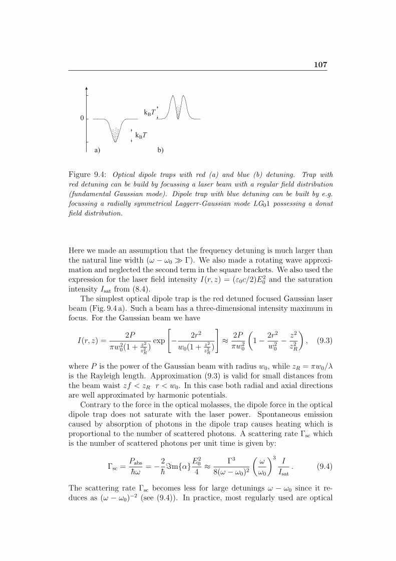
107

Figure 9.4: Optical dipole traps with red (a) and blue (b) detuning. Trap with

red detuning can be build by focussing a laser beam with a regular field distribution

(fundamental Gaussian mode). Dipole trap with blue detuning can be built by e.g.

focussing a radially symmetrical Laggerr-Gaussian mode LG01 possessing a donut

field distribution.

Here we made an assumption that the frequency detuning is much larger thanthe natural line width (ω − ω0 ≫ Γ). We also made a rotating wave approxi-mation and neglected the second term in the square brackets. We also used theexpression for the laser field intensity I(r, z) = (ε0c/2)E

20 and the saturation

intensity Isat from (8.4).The simplest optical dipole trap is the red detuned focused Gaussian laser

beam (Fig. 9.4 a). Such a beam has a three-dimensional intensity maximum infocus. For the Gaussian beam we have

I(r, z) =2P

πw20(1 +

z2

z2R)exp

[− 2r2

w0(1 +z2

z2R)

]≈ 2P

πw20

(1− 2r2

w20

− z2

z2R

), (9.3)

where P is the power of the Gaussian beam with radius w0, while zR = πw0/λis the Rayleigh length. Approximation (9.3) is valid for small distances fromthe beam waist zf < zR r < w0. In this case both radial and axial directionsare well approximated by harmonic potentials.

Contrary to the force in the optical molasses, the dipole force in the opticaldipole trap does not saturate with the laser power. Spontaneous emissioncaused by absorption of photons in the dipole trap causes heating which isproportional to the number of scattered photons. A scattering rate Γsc whichis the number of scattered photons per unit time is given by:

Γsc =Pabs

hω= −2

hℑmαE

20

4≈ Γ3

8(ω − ω0)2

(ω

ω0

)3I

Isat. (9.4)

The scattering rate Γsc becomes less for large detunings ω − ω0 since it re-duces as (ω − ω0)

−2 (see (9.4)). In practice, most regularly used are optical

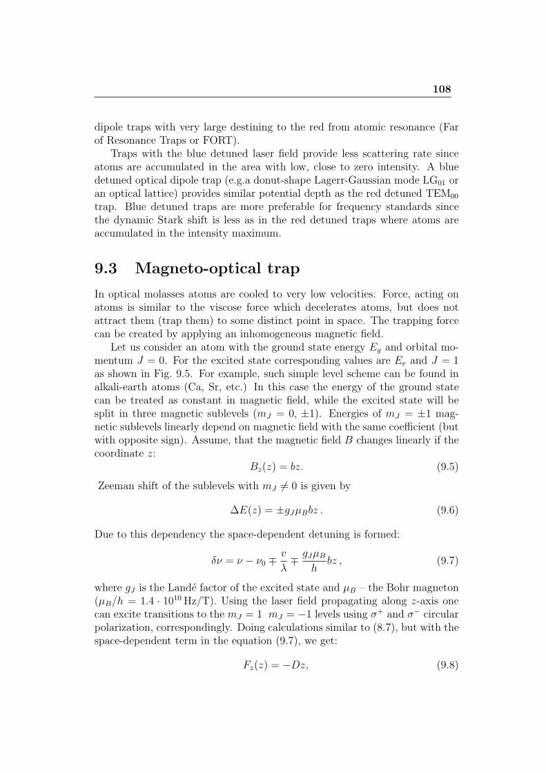
108

dipole traps with very large destining to the red from atomic resonance (Farof Resonance Traps or FORT).

Traps with the blue detuned laser field provide less scattering rate sinceatoms are accumulated in the area with low, close to zero intensity. A bluedetuned optical dipole trap (e.g.a donut-shape Lagerr-Gaussian mode LG01 oran optical lattice) provides similar potential depth as the red detuned TEM00

trap. Blue detuned traps are more preferable for frequency standards sincethe dynamic Stark shift is less as in the red detuned traps where atoms areaccumulated in the intensity maximum.

9.3 Magneto-optical trap

In optical molasses atoms are cooled to very low velocities. Force, acting onatoms is similar to the viscose force which decelerates atoms, but does notattract them (trap them) to some distinct point in space. The trapping forcecan be created by applying an inhomogeneous magnetic field.

Let us consider an atom with the ground state energy Eg and orbital mo-mentum J = 0. For the excited state corresponding values are Ee and J = 1as shown in Fig. 9.5. For example, such simple level scheme can be found inalkali-earth atoms (Ca, Sr, etc.) In this case the energy of the ground statecan be treated as constant in magnetic field, while the excited state will besplit in three magnetic sublevels (mJ = 0, ±1). Energies of mJ = ±1 mag-netic sublevels linearly depend on magnetic field with the same coefficient (butwith opposite sign). Assume, that the magnetic field B changes linearly if thecoordinate z:

Bz(z) = bz. (9.5)

Zeeman shift of the sublevels with mJ = 0 is given by

∆E(z) = ±gJµBbz . (9.6)

Due to this dependency the space-dependent detuning is formed:

δν = ν − ν0 ∓v

λ∓ gJµB

hbz , (9.7)

where gJ is the Lande factor of the excited state and µB – the Bohr magneton(µB/h = 1.4 · 1010Hz/T). Using the laser field propagating along z-axis onecan excite transitions to the mJ = 1 mJ = −1 levels using σ+ and σ− circularpolarization, correspondingly. Doing calculations similar to (8.7), but with thespace-dependent term in the equation (9.7), we get:

Fz(z) = −Dz, (9.8)

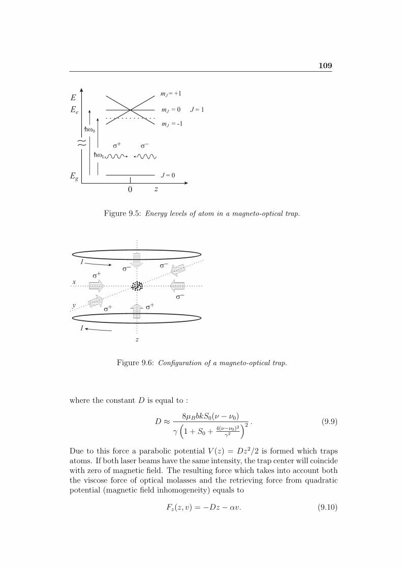
109

Figure 9.5: Energy levels of atom in a magneto-optical trap.

Figure 9.6: Configuration of a magneto-optical trap.

where the constant D is equal to :

D ≈ 8µBbkS0(ν − ν0)

γ(1 + S0 +

4(ν−ν0)2

γ2

)2 . (9.9)

Due to this force a parabolic potential V (z) = Dz2/2 is formed which trapsatoms. If both laser beams have the same intensity, the trap center will coincidewith zero of magnetic field. The resulting force which takes into account boththe viscose force of optical molasses and the retrieving force from quadraticpotential (magnetic field inhomogeneity) equals to

Fz(z, v) = −Dz − αv. (9.10)

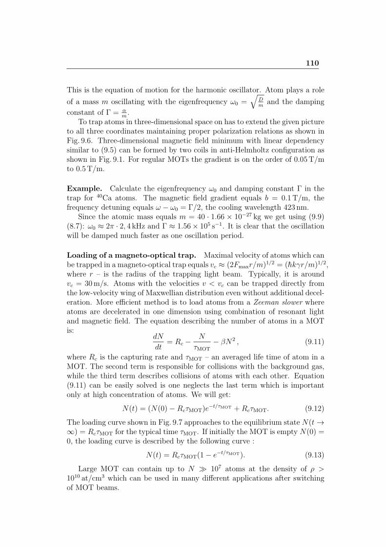
110

This is the equation of motion for the harmonic oscillator. Atom plays a role

of a mass m oscillating with the eigenfrequency ω0 =√

Dm

and the damping

constant of Γ = αm.

To trap atoms in three-dimensional space on has to extend the given pictureto all three coordinates maintaining proper polarization relations as shown inFig. 9.6. Three-dimensional magnetic field minimum with linear dependencysimilar to (9.5) can be formed by two coils in anti-Helmholtz configuration asshown in Fig. 9.1. For regular MOTs the gradient is on the order of 0.05T/mto 0.5T/m.

Example. Calculate the eigenfrequency ω0 and damping constant Γ in thetrap for 40Ca atoms. The magnetic field gradient equals b = 0.1T/m, thefrequency detuning equals ω − ω0 = Γ/2, the cooling wavelength 423 nm.

Since the atomic mass equals m = 40 · 1.66 × 10−27 kg we get using (9.9)(8.7): ω0 ≈ 2π · 2, 4 kHz and Γ ≈ 1.56× 105 s−1. It is clear that the oscillationwill be damped much faster as one oscillation period.

Loading of a magneto-optical trap. Maximal velocity of atoms which canbe trapped in a magneto-optical trap equals vc ≈ (2Fmaxr/m)1/2 = (hkγr/m)1/2,where r – is the radius of the trapping light beam. Typically, it is aroundvc = 30m/s. Atoms with the velocities v < vc can be trapped directly fromthe low-velocity wing of Maxwellian distribution even without additional decel-eration. More efficient method is to load atoms from a Zeeman slower whereatoms are decelerated in one dimension using combination of resonant lightand magnetic field. The equation describing the number of atoms in a MOTis:

dN

dt= Rc −

N

τMOT

− βN2 , (9.11)

where Rc is the capturing rate and τMOT – an averaged life time of atom in aMOT. The second term is responsible for collisions with the background gas,while the third term describes collisions of atoms with each other. Equation(9.11) can be easily solved is one neglects the last term which is importantonly at high concentration of atoms. We will get:

N(t) = (N(0)−RcτMOT)e−t/τMOT +RcτMOT. (9.12)

The loading curve shown in Fig. 9.7 approaches to the equilibrium state N(t→∞) = RcτMOT for the typical time τMOT. If initially the MOT is empty N(0) =0, the loading curve is described by the following curve :

N(t) = RcτMOT(1− e−t/τMOT). (9.13)

Large MOT can contain up to N ≫ 107 atoms at the density of ρ >1010 at/cm3 which can be used in many different applications after switchingof MOT beams.

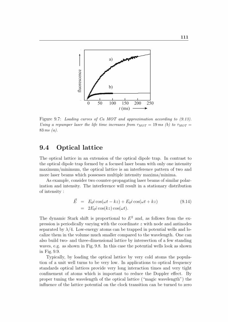
111

Figure 9.7: Loading curves of Ca MOT and approximation according to (9.13).

Using a repumper laser the life time increases from τMOT = 19ms (b) to τMOT =

83ms (a).

9.4 Optical lattice

The optical lattice in an extension of the optical dipole trap. In contrast tothe optical dipole trap formed by a focused laser beam with only one intensitymaximum/minimum, the optical lattice is an interference pattern of two andmore laser beams which possesses multiple intensity maxima/minima.

As example, consider two counter-propagating laser beams of similar polar-ization and intensity. The interference will result in a stationary distributionof intensity :

E = E0ϵ cos(ωt− kz) + E0ϵ cos(ωt+ kz) (9.14)

= 2E0ϵ cos(kz) cos(ωt).

The dynamic Stark shift is proportional to E2 and, as follows from the ex-pression is periodically varying with the coordinate z with node and antinodesseparated by λ/4. Low-energy atoms can be trapped in potential wells and lo-calize them in the volume much smaller compared to the wavelength. One canalso build two- and three-dimensional lattice by intersection of a few standingwaves, e.g. as shown in Fig. 9.8. In this case the potential wells look as shownin Fig. 9.9.

Typically, by loading the optical lattice by very cold atoms the popula-tion of a unit well turns to be very low. In applications to optical frequencystandards optical lattices provide very long interaction times and very tightconfinement of atoms which is important to reduce the Doppler effect. Byproper tuning the wavelength of the optical lattice (“magic wavelength”) theinfluence of the lattice potential on the clock transition can be turned to zero

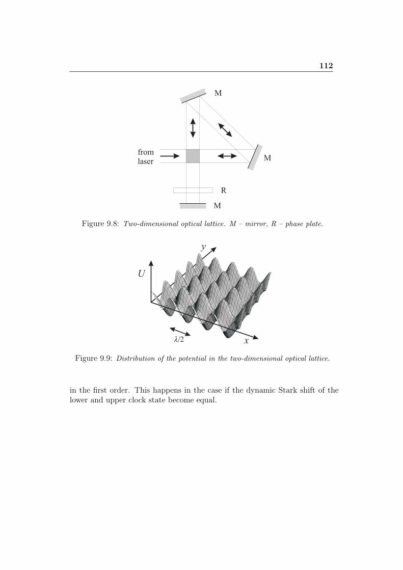
112

Figure 9.8: Two-dimensional optical lattice. M – mirror, R – phase plate.

Figure 9.9: Distribution of the potential in the two-dimensional optical lattice.

in the first order. This happens in the case if the dynamic Stark shift of thelower and upper clock state become equal.

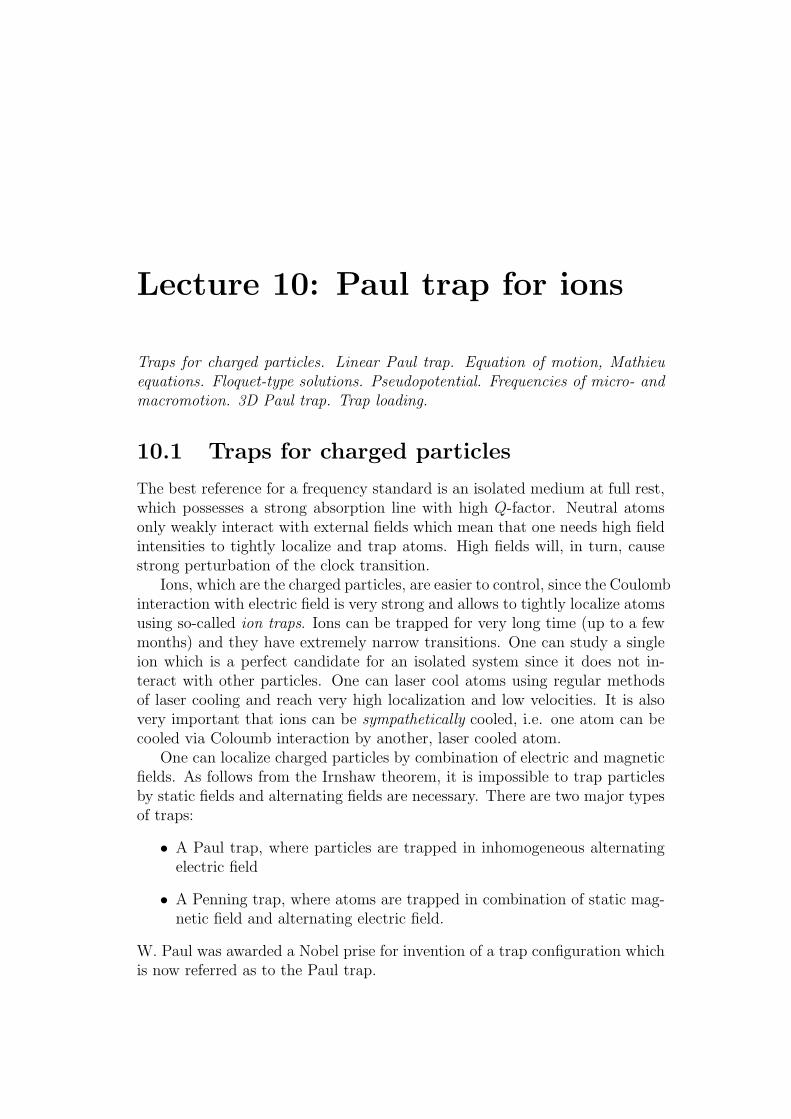
Lecture 10: Paul trap for ions

Traps for charged particles. Linear Paul trap. Equation of motion, Mathieuequations. Floquet-type solutions. Pseudopotential. Frequencies of micro- andmacromotion. 3D Paul trap. Trap loading.

10.1 Traps for charged particles

The best reference for a frequency standard is an isolated medium at full rest,which possesses a strong absorption line with high Q-factor. Neutral atomsonly weakly interact with external fields which mean that one needs high fieldintensities to tightly localize and trap atoms. High fields will, in turn, causestrong perturbation of the clock transition.

Ions, which are the charged particles, are easier to control, since the Coulombinteraction with electric field is very strong and allows to tightly localize atomsusing so-called ion traps. Ions can be trapped for very long time (up to a fewmonths) and they have extremely narrow transitions. One can study a singleion which is a perfect candidate for an isolated system since it does not in-teract with other particles. One can laser cool atoms using regular methodsof laser cooling and reach very high localization and low velocities. It is alsovery important that ions can be sympathetically cooled, i.e. one atom can becooled via Coloumb interaction by another, laser cooled atom.

One can localize charged particles by combination of electric and magneticfields. As follows from the Irnshaw theorem, it is impossible to trap particlesby static fields and alternating fields are necessary. There are two major typesof traps:

• A Paul trap, where particles are trapped in inhomogeneous alternatingelectric field

• A Penning trap, where atoms are trapped in combination of static mag-netic field and alternating electric field.

W. Paul was awarded a Nobel prise for invention of a trap configuration whichis now referred as to the Paul trap.

114

10.2 Paul trap

Consider an electric field E(r) given by potential Φ(r) inside the trap volume.The field interacts with an ion with a charge q = +e =1,602 · 10−19As. Aforce, acting on an ion will be given by

F (r) = eE(r) = −e · ∇Φ(r) , (10.1)

acting towards the trap center. Here the operator ∇ = (∂/∂x, ∂/∂y, ∂/∂z) isused to find the field gradient. It is desirable, that the force will linearly dependon the distance form the trap center r as F (r) ∝ r. In this case particles willundergo harmonic oscillations. In this case a scalar potential Φ(x, y, z) shouldhave a quadratic dependency on coordinates

Φ = const · (ax2 + by2 + cz2) , (10.2)

where the constant is given by boundary conditions. Using the Laplace equa-tion ∆Φ = ∇2 = 0 for a space free of charges, we get the restriction for thecoefficients a, b c defining the potential in (10.2):

a+ b+ c = 0 . (10.3)

We will consider two cases for coefficients (10.3):

a = 1, b = −1, c = 0 (linear quadrupole trap) (10.4)

anda = b = 1, c = −2 (three-dimensional trap). (10.5)

10.3 Linear quadrupole trap

The first combination of coefficients (10.4) describes the trap configurationwith the potential independent on the z-coordinate:

Φ = const · (x2 − y2) . (10.6)

It is a two-dimensional quadrupole potential shown in Fig. 10.1.Such two-dimensional potential (10.6) can be formed by a system of four

hyperbolic electrodes with a negative potential applied to upper and lowerelectrodes and positive - to the right and left electrodes (or vice versa) seeFig. 10.1. Assume, that he potential difference between the electrodes equalsΦ0. The constant from (10.2), (10.6) can be obtained from the boundarycondition Φ(r0) = Φ0/2 = const · r20, where 2r0 is the distance between twoopposite electrodes. We get const = Φ0/2r

20. The electric field is calculated

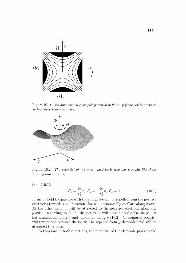
115

Figure 10.1: Two-dimensional qudrupole potential in the x – y plane can be produced

by four hyperbolic electrodes.

Figure 10.2: The potential of the linear quadrupole trap has a saddle-like shape

rotating around z-axis..

from (10.1):

Ex =Φ0

r20x, Ey = −Φ0

r20y, Ez = 0. (10.7)

In such a field the particle with the charge +e will be repelled from the positiveelectrodes towards x = 0 position. Ion will harmonically oscillate along x-axis.At the other hand, it will be attracted to the negative electrode along they-axis. According to (10.6) the potential will have a saddle-like shape. Ithas a minimum along x and maximum along y (10.2). Changing of polaritywill reverse the picture: the ion will be repelled from y-electrodes and will beattracted to x ones.

To trap ions in both directions, the potential of the electrode pairs should

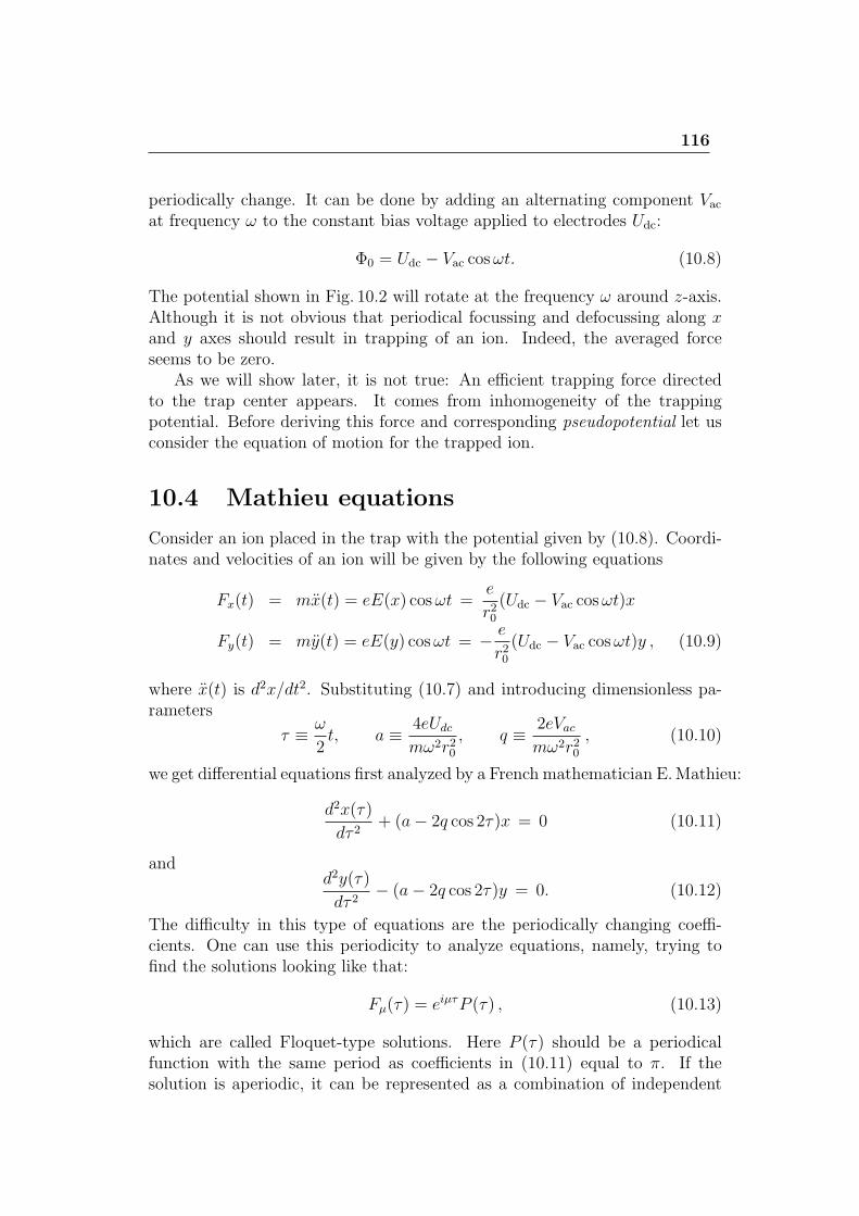
116

periodically change. It can be done by adding an alternating component Vacat frequency ω to the constant bias voltage applied to electrodes Udc:

Φ0 = Udc − Vac cosωt. (10.8)

The potential shown in Fig. 10.2 will rotate at the frequency ω around z-axis.Although it is not obvious that periodical focussing and defocussing along xand y axes should result in trapping of an ion. Indeed, the averaged forceseems to be zero.

As we will show later, it is not true: An efficient trapping force directedto the trap center appears. It comes from inhomogeneity of the trappingpotential. Before deriving this force and corresponding pseudopotential let usconsider the equation of motion for the trapped ion.

10.4 Mathieu equations

Consider an ion placed in the trap with the potential given by (10.8). Coordi-nates and velocities of an ion will be given by the following equations

Fx(t) = mx(t) = eE(x) cosωt =e

r20(Udc − Vac cosωt)x

Fy(t) = my(t) = eE(y) cosωt = − e

r20(Udc − Vac cosωt)y , (10.9)

where x(t) is d2x/dt2. Substituting (10.7) and introducing dimensionless pa-rameters

τ ≡ ω

2t, a ≡ 4eUdc

mω2r20, q ≡ 2eVac

mω2r20, (10.10)

we get differential equations first analyzed by a French mathematician E.Mathieu:

d2x(τ)

dτ 2+ (a− 2q cos 2τ)x = 0 (10.11)

andd2y(τ)

dτ 2− (a− 2q cos 2τ)y = 0. (10.12)

The difficulty in this type of equations are the periodically changing coeffi-cients. One can use this periodicity to analyze equations, namely, trying tofind the solutions looking like that:

Fµ(τ) = eiµτP (τ) , (10.13)

which are called Floquet-type solutions. Here P (τ) should be a periodicalfunction with the same period as coefficients in (10.11) equal to π. If thesolution is aperiodic, it can be represented as a combination of independent

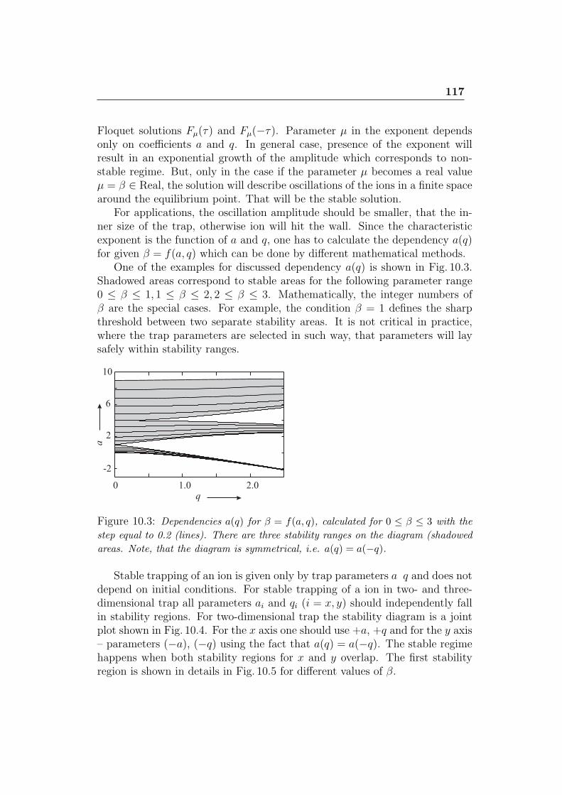
117

Floquet solutions Fµ(τ) and Fµ(−τ). Parameter µ in the exponent dependsonly on coefficients a and q. In general case, presence of the exponent willresult in an exponential growth of the amplitude which corresponds to non-stable regime. But, only in the case if the parameter µ becomes a real valueµ = β ∈ Real, the solution will describe oscillations of the ions in a finite spacearound the equilibrium point. That will be the stable solution.

For applications, the oscillation amplitude should be smaller, that the in-ner size of the trap, otherwise ion will hit the wall. Since the characteristicexponent is the function of a and q, one has to calculate the dependency a(q)for given β = f(a, q) which can be done by different mathematical methods.

One of the examples for discussed dependency a(q) is shown in Fig. 10.3.Shadowed areas correspond to stable areas for the following parameter range0 ≤ β ≤ 1, 1 ≤ β ≤ 2, 2 ≤ β ≤ 3. Mathematically, the integer numbers ofβ are the special cases. For example, the condition β = 1 defines the sharpthreshold between two separate stability areas. It is not critical in practice,where the trap parameters are selected in such way, that parameters will laysafely within stability ranges.

Figure 10.3: Dependencies a(q) for β = f(a, q), calculated for 0 ≤ β ≤ 3 with the

step equal to 0.2 (lines). There are three stability ranges on the diagram (shadowed

areas. Note, that the diagram is symmetrical, i.e. a(q) = a(−q).

Stable trapping of an ion is given only by trap parameters a q and does notdepend on initial conditions. For stable trapping of a ion in two- and three-dimensional trap all parameters ai and qi (i = x, y) should independently fallin stability regions. For two-dimensional trap the stability diagram is a jointplot shown in Fig. 10.4. For the x axis one should use +a, +q and for the y axis– parameters (−a), (−q) using the fact that a(q) = a(−q). The stable regimehappens when both stability regions for x and y overlap. The first stabilityregion is shown in details in Fig. 10.5 for different values of β.

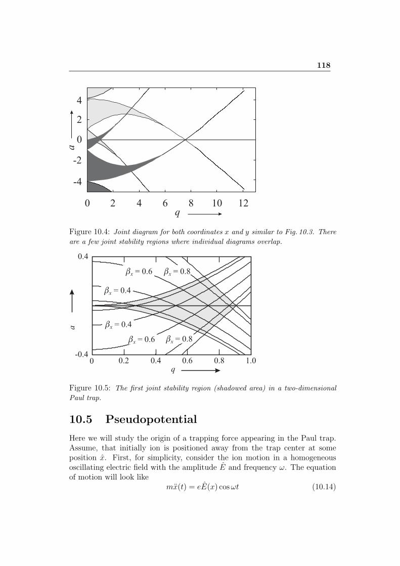
118

Figure 10.4: Joint diagram for both coordinates x and y similar to Fig. 10.3. There

are a few joint stability regions where individual diagrams overlap.

Figure 10.5: The first joint stability region (shadowed area) in a two-dimensional

Paul trap.

10.5 Pseudopotential

Here we will study the origin of a trapping force appearing in the Paul trap.Assume, that initially ion is positioned away from the trap center at someposition x. First, for simplicity, consider the ion motion in a homogeneousoscillating electric field with the amplitude E and frequency ω. The equationof motion will look like

mx(t) = eE(x) cosωt (10.14)

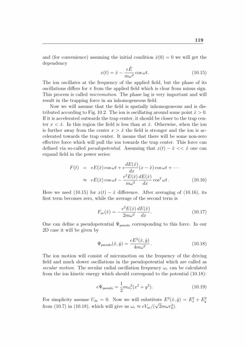
119

and (for convenience) assuming the initial condition x(0) = 0 we will get thedependency

x(t) = x− eE

mω2cosωt. (10.15)

The ion oscillates at the frequency of the applied field, but the phase of itsoscillations differs for π from the applied field which is clear from minus sign.This process is called micromotion. The phase lag is very important and willresult in the trapping force in an inhomogeneous field.

Now we will assume that the field is spatially inhomogeneous and is dis-tributed according to Fig. 10.2. The ion is oscillating around some point x > 0.If it is accelerated outwards the trap center, it should be closer to the trap cen-ter x < x. In this region the field is less than at x. Otherwise, when the ionis further away from the center x > x the field is stronger and the ion is ac-celerated towards the trap center. It means that there will be some non-zeroeffective force which will pull the ion towards the trap center. This force candefined via so-called pseudopotential. Assuming that x(t) − x << x one canexpand field in the power series:

F (t) = eE(x) cosωt+ edE(x)

dx(x− x) cosωt+ · · ·

≈ eE(x) cosωt− e2E(x)

mω2

dE(x)

dxcos2 ωt . (10.16)

Here we used (10.15) for x(t) − x difference. After averaging of (10.16), itsfirst term becomes zero, while the average of the second term is

Fav(x) = −e2E(x)

2mω2

dE(x)

dx. (10.17)

One can define a pseudopotential Ψpseudo corresponding to this force. In our2D case it will be given by

Ψpseudo(x, y) =eE2(x, y)

4mω2. (10.18)

The ion motion will consist of micromotion on the frequency of the drivingfield and much slower oscillations in the pseudopotential which are called assecular motion. The secular radial oscillation frequency ωr can be calculatedfrom the ion kinetic energy which should correspond to the potential (10.18):

eΨpseudo =1

2mω2

r(x2 + y2). (10.19)

For simplicity assume Udc = 0. Now we will substitute E2(x, y) = E2x + E2

y

from (10.7) in (10.18), which will give us ωr ≈ eVac/(√2mωr20).

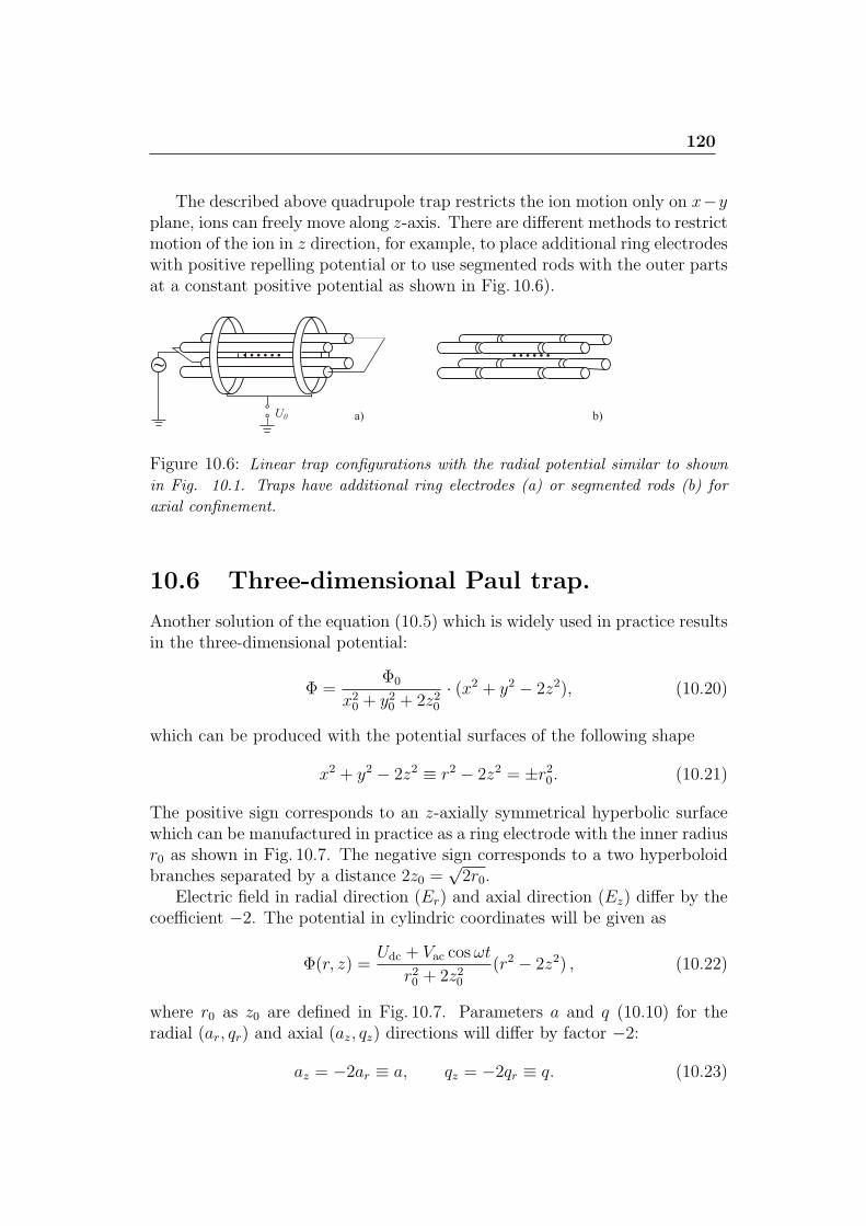
120

The described above quadrupole trap restricts the ion motion only on x−yplane, ions can freely move along z-axis. There are different methods to restrictmotion of the ion in z direction, for example, to place additional ring electrodeswith positive repelling potential or to use segmented rods with the outer partsat a constant positive potential as shown in Fig. 10.6).

Figure 10.6: Linear trap configurations with the radial potential similar to shown

in Fig. 10.1. Traps have additional ring electrodes (a) or segmented rods (b) for

axial confinement.

10.6 Three-dimensional Paul trap.

Another solution of the equation (10.5) which is widely used in practice resultsin the three-dimensional potential:

Φ =Φ0

x20 + y20 + 2z20· (x2 + y2 − 2z2), (10.20)

which can be produced with the potential surfaces of the following shape

x2 + y2 − 2z2 ≡ r2 − 2z2 = ±r20. (10.21)

The positive sign corresponds to an z-axially symmetrical hyperbolic surfacewhich can be manufactured in practice as a ring electrode with the inner radiusr0 as shown in Fig. 10.7. The negative sign corresponds to a two hyperboloidbranches separated by a distance 2z0 =

√2r0.

Electric field in radial direction (Er) and axial direction (Ez) differ by thecoefficient −2. The potential in cylindric coordinates will be given as

Φ(r, z) =Udc + Vac cosωt

r20 + 2z20(r2 − 2z2) , (10.22)

where r0 as z0 are defined in Fig. 10.7. Parameters a and q (10.10) for theradial (ar, qr) and axial (az, qz) directions will differ by factor −2:

az = −2ar ≡ a, qz = −2qr ≡ q. (10.23)

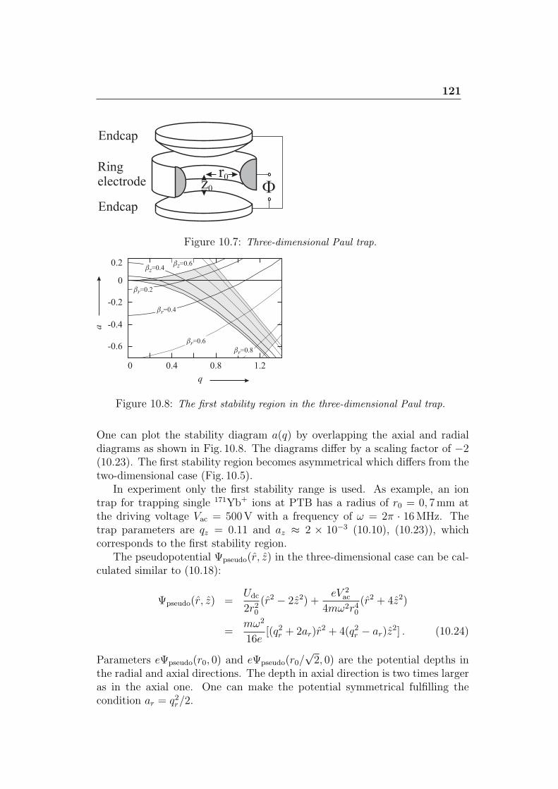
121

Figure 10.7: Three-dimensional Paul trap.

Figure 10.8: The first stability region in the three-dimensional Paul trap.

One can plot the stability diagram a(q) by overlapping the axial and radialdiagrams as shown in Fig. 10.8. The diagrams differ by a scaling factor of −2(10.23). The first stability region becomes asymmetrical which differs from thetwo-dimensional case (Fig. 10.5).

In experiment only the first stability range is used. As example, an iontrap for trapping single 171Yb+ ions at PTB has a radius of r0 = 0, 7mm atthe driving voltage Vac = 500V with a frequency of ω = 2π · 16MHz. Thetrap parameters are qz = 0.11 and az ≈ 2 × 10−3 (10.10), (10.23)), whichcorresponds to the first stability region.

The pseudopotential Ψpseudo(r, z) in the three-dimensional case can be cal-culated similar to (10.18):

Ψpseudo(r, z) =Udc

2r20(r2 − 2z2) +

eV 2ac

4mω2r40(r2 + 4z2)

=mω2

16e[(q2r + 2ar)r

2 + 4(q2r − ar)z2] . (10.24)

Parameters eΨpseudo(r0, 0) and eΨpseudo(r0/√2, 0) are the potential depths in

the radial and axial directions. The depth in axial direction is two times largeras in the axial one. One can make the potential symmetrical fulfilling thecondition ar = q2r/2.

Lecture 11: Penning trap forions and ion cooling

Penning trap for charged particles. Magnetron, cyclotron and axial frequencies.Precision mass comparison in the Penning trap. Synthesis of anti-hydrogenatoms in Penning traps. Cooling of ions. Doppler and sideband cooling. Sym-pathetic cooling. Lamb-Dicke regime.

11.1 Penning trap

Configuration of electrodes in the Penning trap is the same as in the 3D Paultrap, but the radio-frequency field is absent (Vac = 0). It means that ionswill repel from the end cap electrodes (along z direction). In the x – y planethe same potential will push ions out of the trap center. For trapping ions astrong magnetic field is applied along z-axis. Equation of electron motion canbe written as

m¨r = eE(r) + e ˙r × B, which is equivalent (11.1)

mx = e(Er + yBz)

my = e(Er − xBz)

mz = eEz.

The electrical field components can be calculated from the potential Φ (10.22).The last equation describes ion oscillations with the frequency of

ω2z =

4eUdc

m(r20 + 2z20), (11.2)

which does not depend on Bz.If only magnetic field is applied to a moving particle, it will perform a cir-

cular motion in the plane orthogonal to the field. The frequency of oscillationswill be given by

ωc =e

mBz (cyclotron frequncy). (11.3)

The cyclotron frequency can be obtained from the fact that the Lorentzforces provides the centripetal acceleration evBz = mv2/r or eBz = mωc. In

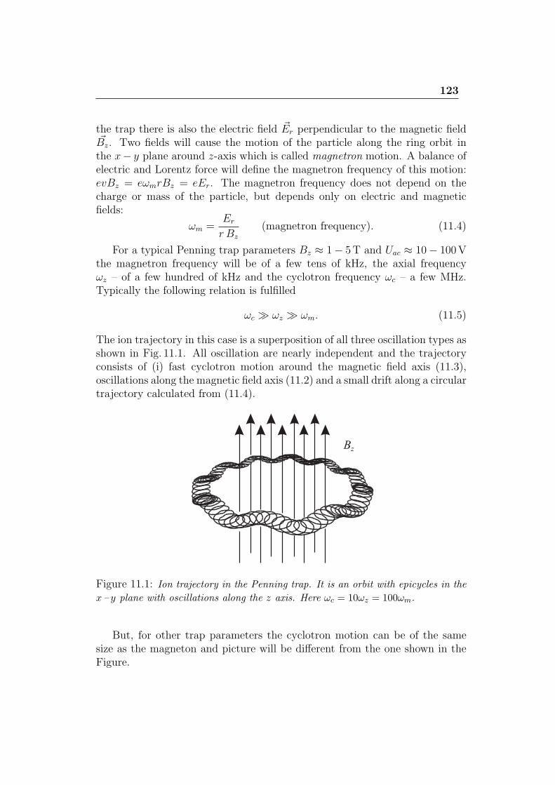
123

the trap there is also the electric field Er perpendicular to the magnetic fieldBz. Two fields will cause the motion of the particle along the ring orbit inthe x− y plane around z-axis which is called magnetron motion. A balance ofelectric and Lorentz force will define the magnetron frequency of this motion:evBz = eωmrBz = eEr. The magnetron frequency does not depend on thecharge or mass of the particle, but depends only on electric and magneticfields:

ωm =Er

r Bz

(magnetron frequency). (11.4)

For a typical Penning trap parameters Bz ≈ 1− 5T and Uac ≈ 10− 100Vthe magnetron frequency will be of a few tens of kHz, the axial frequencyωz – of a few hundred of kHz and the cyclotron frequency ωc – a few MHz.Typically the following relation is fulfilled

ωc ≫ ωz ≫ ωm. (11.5)

The ion trajectory in this case is a superposition of all three oscillation types asshown in Fig. 11.1. All oscillation are nearly independent and the trajectoryconsists of (i) fast cyclotron motion around the magnetic field axis (11.3),oscillations along the magnetic field axis (11.2) and a small drift along a circulartrajectory calculated from (11.4).

Figure 11.1: Ion trajectory in the Penning trap. It is an orbit with epicycles in the

x – y plane with oscillations along the z axis. Here ωc = 10ωz = 100ωm.

But, for other trap parameters the cyclotron motion can be of the samesize as the magneton and picture will be different from the one shown in theFigure.

124

11.1.1 Rigorous solution

One can rigorously solve joint differential equations (11.1) for x and y:

x =e

m

(2Udc

r20 + 2z20x+ yBz

)=ω2z

2x+ ωcy (11.6)

y =e

m

(2Udc

r20 + 2z20y − xBz

)=ω2z

2x− ωcx. (11.7)

Let us add equation (11.6) to equation (11.7) multiplied by i. Also we introducecomplex parameter r = x + iy. After this procedure we will get a simplifiedequation r = ω2

zr/2 − iωcr. It can be solved by substitution r = r0 exp(iωt)which will result in a square equation ω2 − ωωc − ω2

z/2 = 0 for ω. Two rootsof this equation will give us frequencies

ω′c =

ωc

2+

√ω2c

4− ω2

z

2(modified cyclotron frequency) (11.8)

ωm =ωc

2−√ω2c

4− ω2

z

2(magnetron frequency). (11.9)

If the value under the square root is positive (ωc ≥√2ωz), we will get two

frequencies called as modified cyclotron frequency ω′c and magnetron frequency

ωm. Modification of the original cyclotron frequency comes from the presenceof electric field.

One can also get important relations by (i) adding the equations (11.8) and(11.9) or (ii) by squaring them and then adding them. As a result we get:

ωc = ω′c + ωm (11.10)

ω2c = ω′2

c + ω2m + ω2

z . (11.11)

Both these frequencies are used to calculate the cyclotron frequency (11.3)which is very important for precision ion mass comparison.

For a cloud of ions in the Penning trap, fast magnetron motion along(E × B) results in Doppler effect second order. For larger cloud size the effectis larger. Penning traps are not often used for optical or microwave frequencystandards and are inferior to Paul traps. But they become very important toolfor many fundamental applications like precision mass comparison, determina-tion of anomalous magnetic moment of electron and producing antihydrogenatoms.

11.1.2 Ion energies in the Penning trap.

Consider an single-charged ion (m = 100 a.u.) moving in the Paul trap withthe potential difference of 10 V, B = 5T and r = 1mm. Which energycorresponds to each type of ion motion?

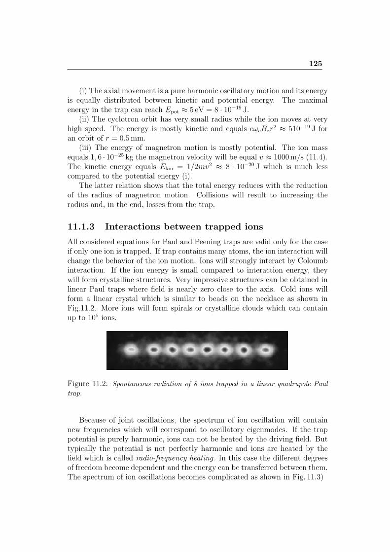
125

(i) The axial movement is a pure harmonic oscillatory motion and its energyis equally distributed between kinetic and potential energy. The maximalenergy in the trap can reach Epot ≈ 5 eV = 8 · 10−19 J.

(ii) The cyclotron orbit has very small radius while the ion moves at veryhigh speed. The energy is mostly kinetic and equals eωcBzr

2 ≈ 510−19 J foran orbit of r = 0.5mm.

(iii) The energy of magnetron motion is mostly potential. The ion massequals 1, 6 · 10−25 kg the magnetron velocity will be equal v ≈ 1000m/s (11.4).The kinetic energy equals Ekin = 1/2mv2 ≈ 8 · 10−20 J which is much lesscompared to the potential energy (i).

The latter relation shows that the total energy reduces with the reductionof the radius of magnetron motion. Collisions will result to increasing theradius and, in the end, losses from the trap.

11.1.3 Interactions between trapped ions

All considered equations for Paul and Peening traps are valid only for the caseif only one ion is trapped. If trap contains many atoms, the ion interaction willchange the behavior of the ion motion. Ions will strongly interact by Coloumbinteraction. If the ion energy is small compared to interaction energy, theywill form crystalline structures. Very impressive structures can be obtained inlinear Paul traps where field is nearly zero close to the axis. Cold ions willform a linear crystal which is similar to beads on the necklace as shown inFig.11.2. More ions will form spirals or crystalline clouds which can containup to 105 ions.

Figure 11.2: Spontaneous radiation of 8 ions trapped in a linear quadrupole Paul

trap.

Because of joint oscillations, the spectrum of ion oscillation will containnew frequencies which will correspond to oscillatory eigenmodes. If the trappotential is purely harmonic, ions can not be heated by the driving field. Buttypically the potential is not perfectly harmonic and ions are heated by thefield which is called radio-frequency heating. In this case the different degreesof freedom become dependent and the energy can be transferred between them.The spectrum of ion oscillations becomes complicated as shown in Fig. 11.3)

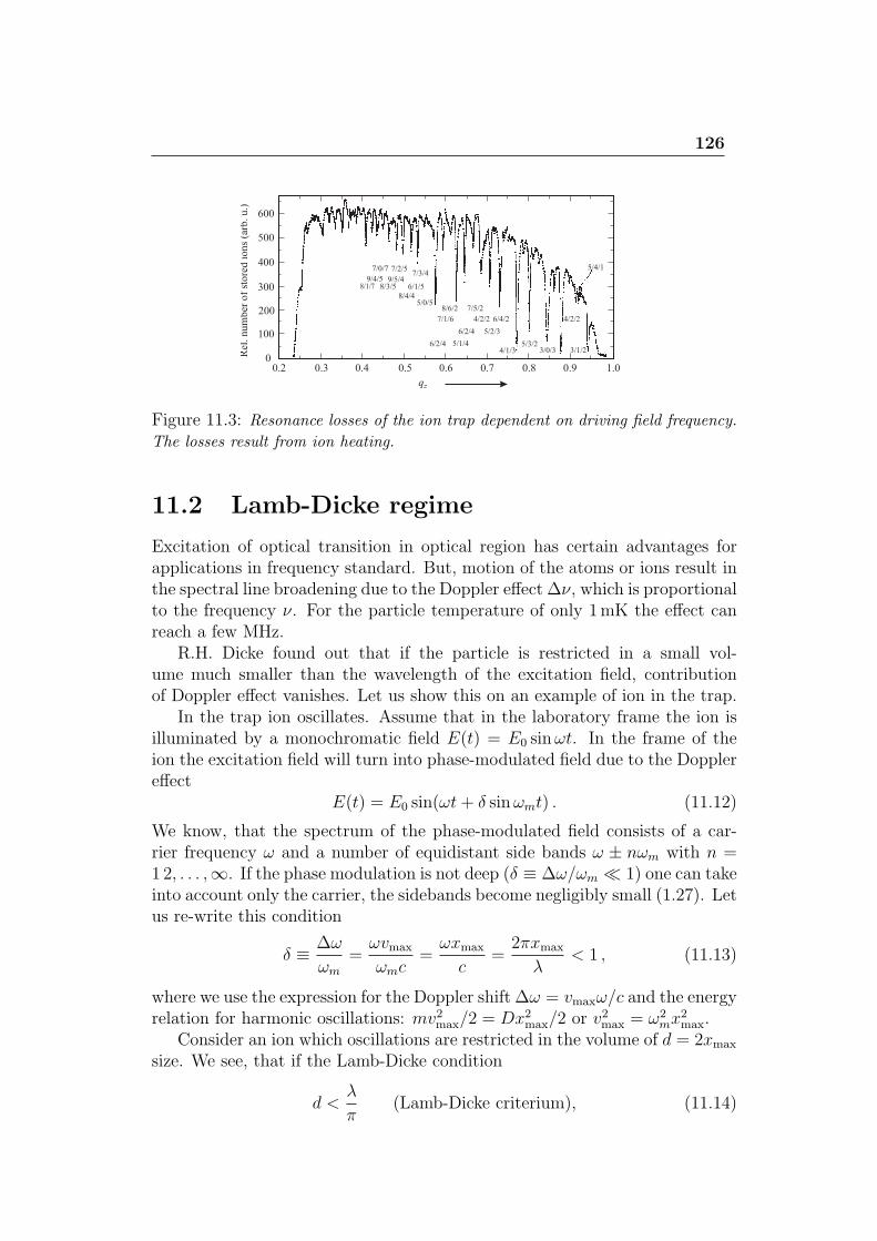
126

Figure 11.3: Resonance losses of the ion trap dependent on driving field frequency.

The losses result from ion heating.

11.2 Lamb-Dicke regime

Excitation of optical transition in optical region has certain advantages forapplications in frequency standard. But, motion of the atoms or ions result inthe spectral line broadening due to the Doppler effect ∆ν, which is proportionalto the frequency ν. For the particle temperature of only 1mK the effect canreach a few MHz.

R.H. Dicke found out that if the particle is restricted in a small vol-ume much smaller than the wavelength of the excitation field, contributionof Doppler effect vanishes. Let us show this on an example of ion in the trap.

In the trap ion oscillates. Assume that in the laboratory frame the ion isilluminated by a monochromatic field E(t) = E0 sinωt. In the frame of theion the excitation field will turn into phase-modulated field due to the Dopplereffect

E(t) = E0 sin(ωt+ δ sinωmt) . (11.12)

We know, that the spectrum of the phase-modulated field consists of a car-rier frequency ω and a number of equidistant side bands ω ± nωm with n =12, . . . ,∞. If the phase modulation is not deep (δ ≡ ∆ω/ωm ≪ 1) one can takeinto account only the carrier, the sidebands become negligibly small (1.27). Letus re-write this condition

δ ≡ ∆ω

ωm

=ωvmax

ωmc=ωxmax

c=

2πxmax

λ< 1 , (11.13)

where we use the expression for the Doppler shift ∆ω = vmaxω/c and the energyrelation for harmonic oscillations: mv2max/2 = Dx2max/2 or v2max = ω2

mx2max.

Consider an ion which oscillations are restricted in the volume of d = 2xmax

size. We see, that if the Lamb-Dicke condition

d <λ

π(Lamb-Dicke criterium), (11.14)

127

is fulfilled, then according to (11.13) the condition δ < 1 is also fulfilled.The more strict condition (11.14) is fulfilled, the less the Doppler broaden-

ing of the spectral line. Radiation will be mostly absorbed ion the carrier andnot in the sidebands. This criterium is also valid for any particle restricted inthe volume of the size less than the wavelength of the excitation field. It isimportant in ion traps, optical lattices and hydrogen masers.

11.3 Trap loading

Loading of the ion trap significantly differs from loading of a magneto-opticaltrap because of absence of any dissipative force. It means, that the particleenergy should be less than the energy barrier of the trap itself and the trapcannot be loaded from outside. It is similar to the case that the planet cannotbe trapped to the stable orbit if it comes from infinity. To be trappable, thebody should experience some collision or be born close to the potential wellcenter.

There are a few methods how to load ions in the trap. The most usualone is the ionization of neutral atoms directly inside the trap, for example, byelectron bombardment. Neutral particles easily penetrate to the trap centerwithout interaction with magnetic and electric field. After impact with theelectron, neutral particle becomes ionized, and if its energy is low enough,would be trapped in the ion trap. The similar method is photo-ionizationwhich is isotope-selective and causes less induced charges on the trap walls.

This method cannot be used if one traps anti-particles or exotic isotopesfrom the accelerator ring. In this case one can lower the potential barrier atone side of the trap, then load the trap, and, as soon as ions are inside, liftup the barrier again. Of course, it should be done very fast, before ions arereflected from the other side of the trap.

11.4 Ion cooling

Ion traps can trap ions at high energies up to 2 eV which corresponds to tem-peratures of 20 000K. Even the second order Doppler effect of such particleswill be huge ∆ν/ν = −v2/(2c2) = −(mv2/2)/(mc2) ≈ −2 eV ≈ −10−11, whichis too much for any applications in the frequency standards. Since ions in theion trap are nearly completely isolated, thermalization is inefficient and ionsshould be cooled by some other methods. Isolation from the environment hasalso a lot of advantages: As soon as ions are cooled, they will not be heatedfor the long time.

We should agree about notation “temperature” which is appied in this caseto a single ion. We will stick to the standard agreement that temperature Twill define the energy of ion per degree of freedom : Ei = kT/2.

128

11.4.1 Energy dissipation by an electric circuit

Ions, oscillating in a trap, induce mirror charges and corresponding currentsin the electrodes. If electrodes are shunted by a resistor, ion will loose energyand its oscillations will dissipate. In the limit, ion temperature will be givenby shunt resistor temperature.

Dissipation rate of ion in the trap with the shunt circuit. Assume,that an ion with mass m and the charge q oscillates along z-axis at a distanceof 2z0 from each other as shown in Fig. 10.7. Resistance of the shunt is R.Derive the energy dissipation rate of an ion.

If ion with velocity v is moving for the distance ds in the electric field E,the energy gain/loss will be equal to dWz = qEds.

Corresponding power equals dWz/dt = qEds/dt ≈ qUv/(2z0). Currentflowing between electrodes can be derived from the following relation IU =qUv/(2z0), which means I = qv/(2z0). This approximation corresponds to thecase if the trap electrodes can be considered as plane capacitor.

The equivalent electric circuit is a current source connected to the planecapacitor via resistor R. The averaged power scattered on resistor equals⟨I2R⟩. In the case if the capacitance is small R ≪ 1/(ωzC), the averagedpower, dissipated by an ion can be calculated as

−dWz

dt= ⟨I2R⟩ = q2RWz

4mz20, (11.15)

where we used the relation Wz = m⟨v2z⟩ for the ion kinetic energy. Solutionof this equation described the exponential power dissipation which the timeconstant of

t0 =4mz20q2R

. (11.16)

This cooling method can be used for any ion. Usually, the trap electrodes areshunted by resistor which is cooled in liquid nitrogen or helium. It allows tocool ions to temperatures down to 1 K. For example, such cooling is used forpositron cooling for production of anti-hydrogen.

11.4.2 Buffer gas cooling

The easiest way to cool atoms in the trap is to add some buffer gas in thevacuum volume. Since the trap depth is very high, collisions with a trappedion will take energy from it without knocking it out of the trap. Each collisionbetween the ion and buffer gas atom will reduce the energy of the ion by

∆Ekin

Ekin

=mbuffer

mion

. (11.17)

One can cool ions to temperatures down to 4K if cryogenic trap is used.

129

11.4.3 Doppler laser cooling

First who suggested laser cooling of ions in the trap were Weinland and Demeltin 1975. The Doppler cooling method is very similar to laser cooling of atomsin optical molasses. It relies on absorption of the photon which the energylower than energy of emitted one (at average). The energy difference is takenfrom kinetic energy of a particle.

For ions, the typical resonance lines are quite strong (natural line width10MHz) and allow for efficient ion cooling. Laser cooling of an ion is technicallyless challenging compared to a free particle cooling, because cooling only fromone direction is enough. Preferably ion will absorb photons when it movesopposite to a k-vector of a red-detuned cooling laser field and will loose energycorrespondingly. Typically, only one retro-reflected laser beam is used withdirection intersects with all degrees of freedom of moving ion.

Using this method one can reach the lowest temperature correspondingto the Doppler limit kTD ≡ hγ/2 (see. (8.12)). The minimal temperature isachieved when the frequency detuning is half of the resonance line width γ/2.Typically, one can reach temperatures of TD ≈ 1mK. This method can beused both in Paul and Penning traps.

If many ions are trapped, the heating due to Coloumb repulsion and corre-sponding increased potential inharmonicity will increase the heating rate whichwill result in higher temperatures. There are other heating mechanisms result-ing from interaction of ions with patch charges on electrodes and influence ofelectrical noises of electrodes which may additionally heat ions.

The Doppler temperature is typically enough to obtain crystalline struc-tures in the trap as shown in Fig. 11.2. Still, for many applications the tem-perature is not low enough.

Sideband cooling

The Doppler mechanism for ions and neutral particles are very similar. Thesub-Doppler mechanisms, in turn, differ very much. For neutral particles oneuses Sisyphus or polarization gradient methods where atom either climb thepotential lattice formed due to the dynamical Stark shift or are cooled due toredistribution of population.

For ions sub-Doppler cooling relies on the fact, that an ion is trappedin the potential well and populates some vibrational levels of this trap. Ifpotential is harmonic, its energy levels will be equidistant as shown in Fig. 11.4.Each of the electronic energy levels can be treated as a number of sublevelsseparated by the harmonic trap eigenfrequency. In other words, the oscillatingion will emit a phase-modulated field with the modulation frequency of theoscillations. The spectrum can be approximated by ν0 ± kνm, where ν0 is theion electronic transition frequency, νm is the oscillation frequency and k is thepositive integer.

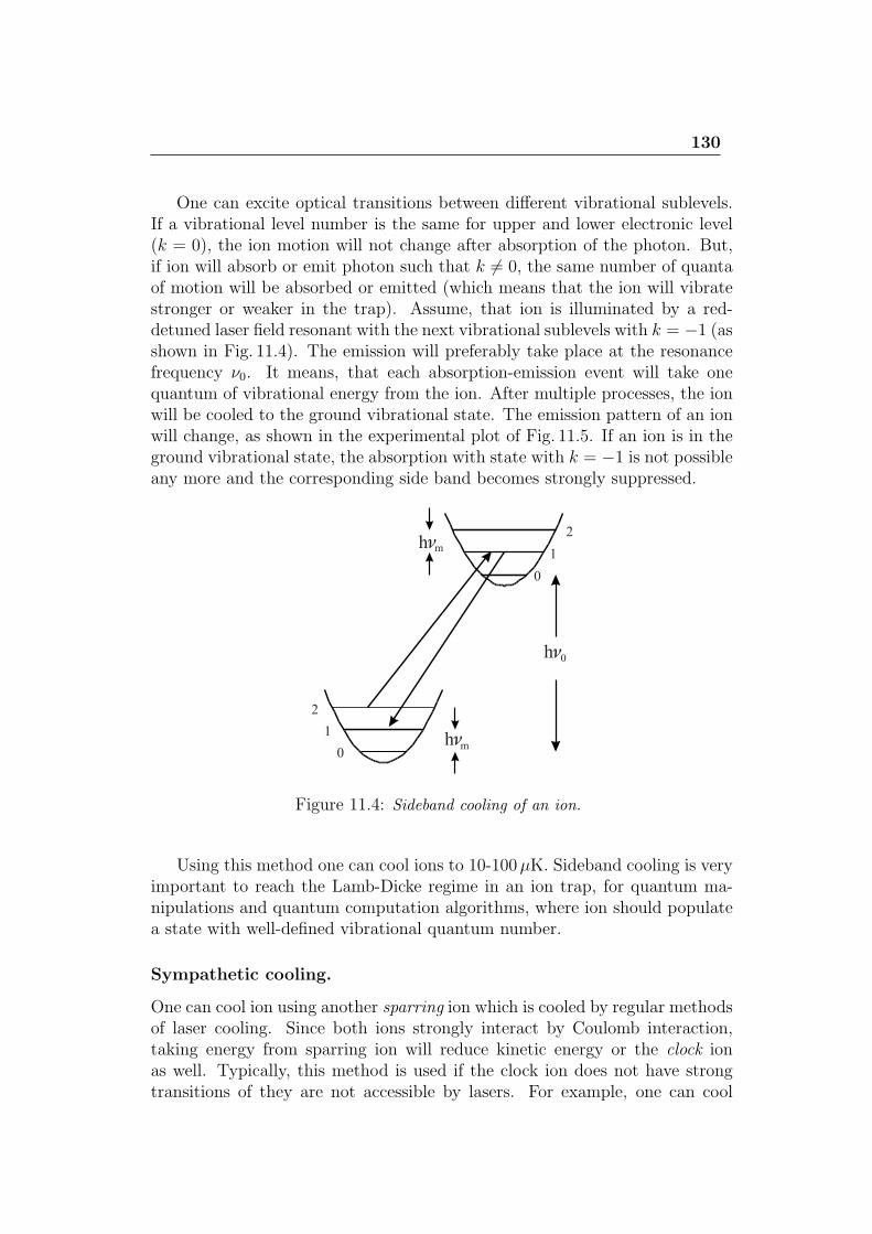
130

One can excite optical transitions between different vibrational sublevels.If a vibrational level number is the same for upper and lower electronic level(k = 0), the ion motion will not change after absorption of the photon. But,if ion will absorb or emit photon such that k = 0, the same number of quantaof motion will be absorbed or emitted (which means that the ion will vibratestronger or weaker in the trap). Assume, that ion is illuminated by a red-detuned laser field resonant with the next vibrational sublevels with k = −1 (asshown in Fig. 11.4). The emission will preferably take place at the resonancefrequency ν0. It means, that each absorption-emission event will take onequantum of vibrational energy from the ion. After multiple processes, the ionwill be cooled to the ground vibrational state. The emission pattern of an ionwill change, as shown in the experimental plot of Fig. 11.5. If an ion is in theground vibrational state, the absorption with state with k = −1 is not possibleany more and the corresponding side band becomes strongly suppressed.

Figure 11.4: Sideband cooling of an ion.

Using this method one can cool ions to 10-100µK. Sideband cooling is veryimportant to reach the Lamb-Dicke regime in an ion trap, for quantum ma-nipulations and quantum computation algorithms, where ion should populatea state with well-defined vibrational quantum number.

Sympathetic cooling.

One can cool ion using another sparring ion which is cooled by regular methodsof laser cooling. Since both ions strongly interact by Coulomb interaction,taking energy from sparring ion will reduce kinetic energy or the clock ionas well. Typically, this method is used if the clock ion does not have strongtransitions of they are not accessible by lasers. For example, one can cool

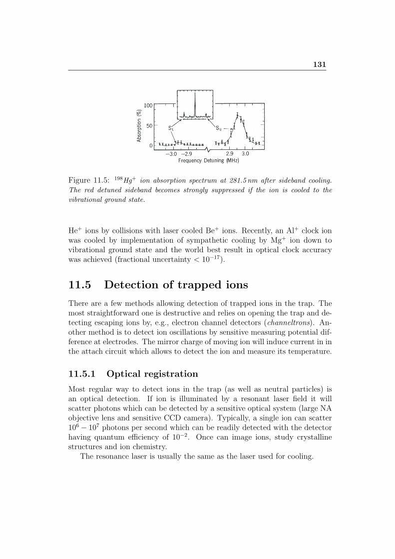
131

Figure 11.5: 198Hg+ ion absorption spectrum at 281.5 nm after sideband cooling.

The red detuned sideband becomes strongly suppressed if the ion is cooled to the

vibrational ground state.

He+ ions by collisions with laser cooled Be+ ions. Recently, an Al+ clock ionwas cooled by implementation of sympathetic cooling by Mg+ ion down tovibrational ground state and the world best result in optical clock accuracywas achieved (fractional uncertainty < 10−17).

11.5 Detection of trapped ions

There are a few methods allowing detection of trapped ions in the trap. Themost straightforward one is destructive and relies on opening the trap and de-tecting escaping ions by, e.g., electron channel detectors (channeltrons). An-other method is to detect ion oscillations by sensitive measuring potential dif-ference at electrodes. The mirror charge of moving ion will induce current in inthe attach circuit which allows to detect the ion and measure its temperature.

11.5.1 Optical registration

Most regular way to detect ions in the trap (as well as neutral particles) isan optical detection. If ion is illuminated by a resonant laser field it willscatter photons which can be detected by a sensitive optical system (large NAobjective lens and sensitive CCD camera). Typically, a single ion can scatter106 − 107 photons per second which can be readily detected with the detectorhaving quantum efficiency of 10−2. Once can image ions, study crystallinestructures and ion chemistry.

The resonance laser is usually the same as the laser used for cooling.

Lecture 12: Methods ofquantum logic in optical clocks

Precision measurements in the traps, electron shelving. Elements of quantumlogic in ion traps. Motional degrees of freedom. CNOT gate. Cirac-Zoller gate.Information transfer between clock and cooling ions. Precision spectroscopyusing quantum logic.

Ions are widely used as frequency standards because of the following reasons

• one can trap single ion which does not interact with other ions

• ion is trapped in the zero of electric potential: no external fields canperturb clock transitions

• ions can be laser cooled to the Lamb-Dicke regime

• ions possess very high-Q transitions in the microwave and optical regions

Ions, which are most successfully used in optical frequency standards are Hg+,Al+, Yb+, Sr+.

Trapped ions are also widely used as elements of quantum logic — themost successive and impressive results were obtained using ions. Here are thereasons why they are also very attractive for this field

• one can address individual ions by tight focussing of light on it

• the interaction between two ions in the trap is strong, while the isolationfrom the environment is nearly perfect. This Coulomb interaction is usedfor quantum gates which is the basic unit of the quantum circuit

• one can store quantum information and increase number of trapped ions(scalability)

For applications in quantum logic circuits one-electron Be+, Mg+ and Ca+ ionsare used.

Here we will consider some modern methods of precision measurements inthe ion traps and some elements of quantum logic.

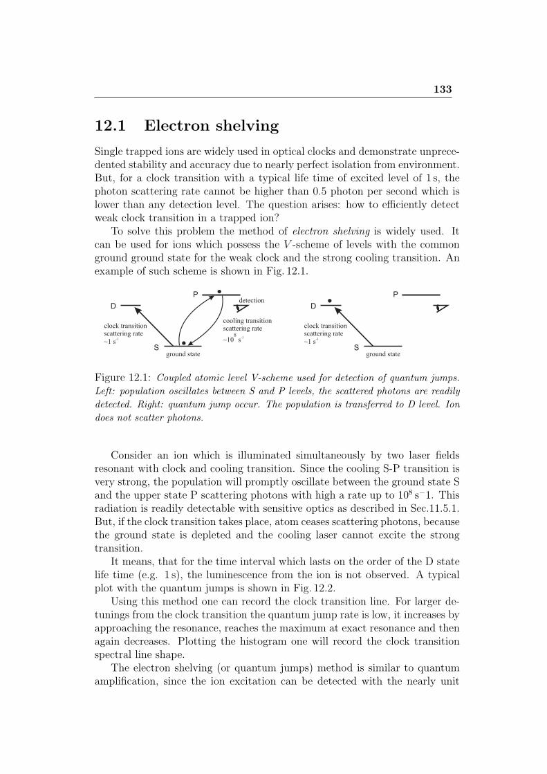
133

12.1 Electron shelving

Single trapped ions are widely used in optical clocks and demonstrate unprece-dented stability and accuracy due to nearly perfect isolation from environment.But, for a clock transition with a typical life time of excited level of 1 s, thephoton scattering rate cannot be higher than 0.5 photon per second which islower than any detection level. The question arises: how to efficiently detectweak clock transition in a trapped ion?

To solve this problem the method of electron shelving is widely used. Itcan be used for ions which possess the V -scheme of levels with the commonground ground state for the weak clock and the strong cooling transition. Anexample of such scheme is shown in Fig. 12.1.

Figure 12.1: Coupled atomic level V-scheme used for detection of quantum jumps.

Left: population oscillates between S and P levels, the scattered photons are readily

detected. Right: quantum jump occur. The population is transferred to D level. Ion

does not scatter photons.

Consider an ion which is illuminated simultaneously by two laser fieldsresonant with clock and cooling transition. Since the cooling S-P transition isvery strong, the population will promptly oscillate between the ground state Sand the upper state P scattering photons with high a rate up to 108 s−1. Thisradiation is readily detectable with sensitive optics as described in Sec.11.5.1.But, if the clock transition takes place, atom ceases scattering photons, becausethe ground state is depleted and the cooling laser cannot excite the strongtransition.

It means, that for the time interval which lasts on the order of the D statelife time (e.g. 1 s), the luminescence from the ion is not observed. A typicalplot with the quantum jumps is shown in Fig. 12.2.

Using this method one can record the clock transition line. For larger de-tunings from the clock transition the quantum jump rate is low, it increases byapproaching the resonance, reaches the maximum at exact resonance and thenagain decreases. Plotting the histogram one will record the clock transitionspectral line shape.

The electron shelving (or quantum jumps) method is similar to quantumamplification, since the ion excitation can be detected with the nearly unit

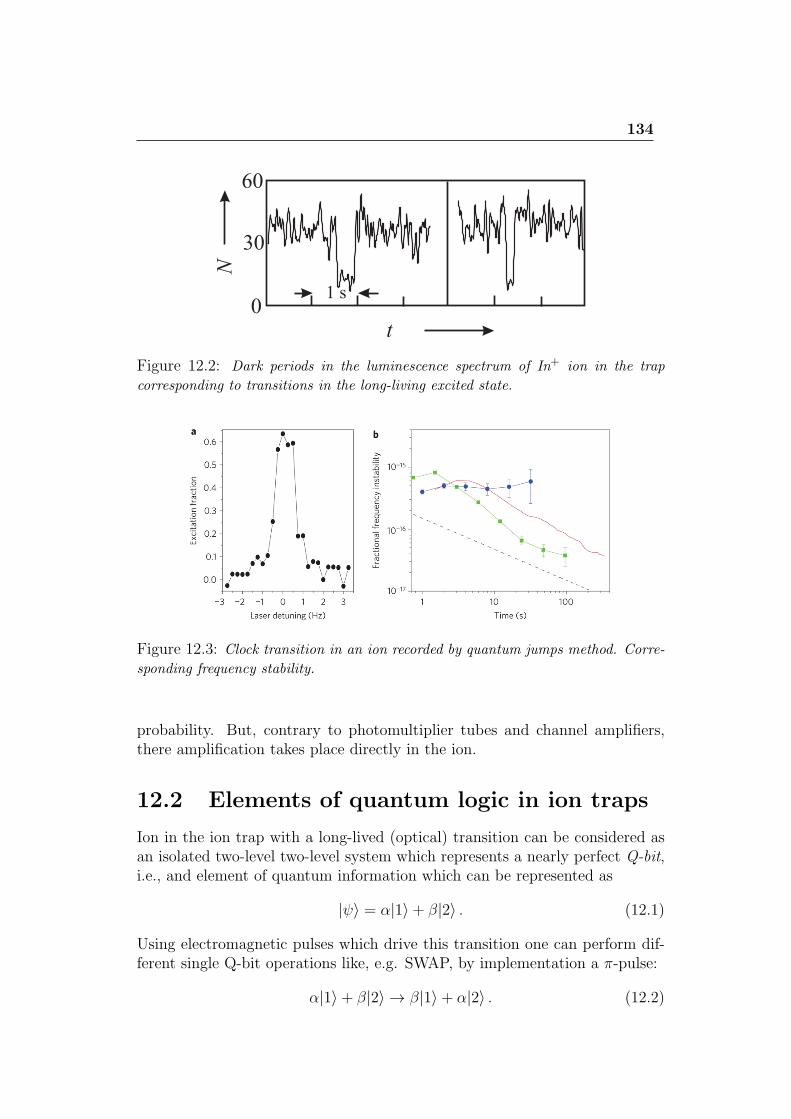
134

Figure 12.2: Dark periods in the luminescence spectrum of In+ ion in the trap

corresponding to transitions in the long-living excited state.

Figure 12.3: Clock transition in an ion recorded by quantum jumps method. Corre-

sponding frequency stability.

probability. But, contrary to photomultiplier tubes and channel amplifiers,there amplification takes place directly in the ion.

12.2 Elements of quantum logic in ion traps

Ion in the ion trap with a long-lived (optical) transition can be considered asan isolated two-level two-level system which represents a nearly perfect Q-bit,i.e., and element of quantum information which can be represented as

|ψ⟩ = α|1⟩+ β|2⟩ . (12.1)

Using electromagnetic pulses which drive this transition one can perform dif-ferent single Q-bit operations like, e.g. SWAP, by implementation a π-pulse:

α|1⟩+ β|2⟩ → β|1⟩+ α|2⟩ . (12.2)

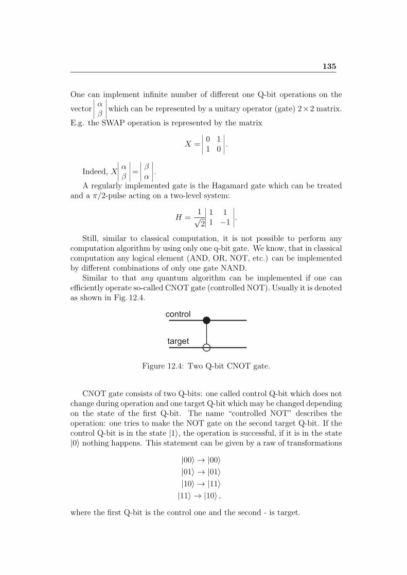
135

One can implement infinite number of different one Q-bit operations on the

vectorαβ

which can be represented by a unitary operator (gate) 2×2 matrix.

E.g. the SWAP operation is represented by the matrix

X =0 11 0

.

Indeed, Xαβ

=βα

.

A regularly implemented gate is the Hagamard gate which can be treatedand a π/2-pulse acting on a two-level system:

H =1√2

1 11 −1

.

Still, similar to classical computation, it is not possible to perform anycomputation algorithm by using only one q-bit gate. We know, that in classicalcomputation any logical element (AND, OR, NOT, etc.) can be implementedby different combinations of only one gate NAND.

Similar to that any quantum algorithm can be implemented if one canefficiently operate so-called CNOT gate (controlled NOT). Usually it is denotedas shown in Fig. 12.4.

Figure 12.4: Two Q-bit CNOT gate.

CNOT gate consists of two Q-bits: one called control Q-bit which does notchange during operation and one target Q-bit which may be changed dependingon the state of the first Q-bit. The name “controlled NOT” describes theoperation: one tries to make the NOT gate on the second target Q-bit. If thecontrol Q-bit is in the state |1⟩, the operation is successful, if it is in the state|0⟩ nothing happens. This statement can be given by a raw of transformations

|00⟩ → |00⟩|01⟩ → |01⟩|10⟩ → |11⟩|11⟩ → |10⟩ ,

where the first Q-bit is the control one and the second - is target.

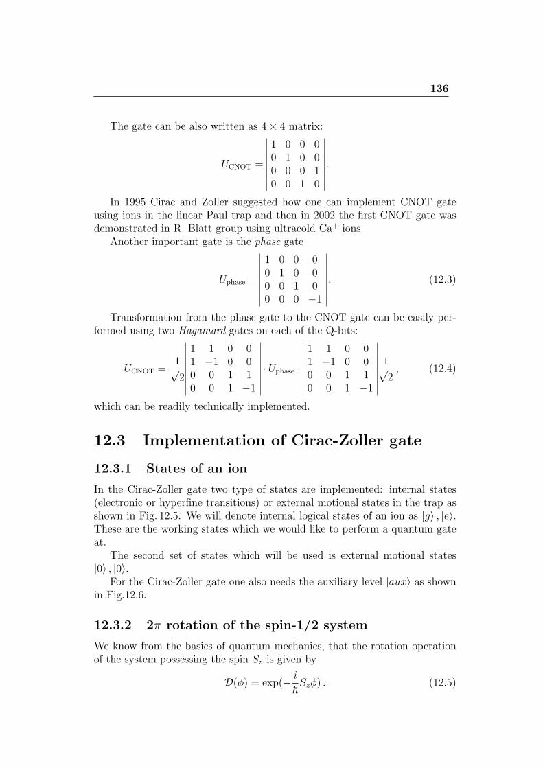
136

The gate can be also written as 4× 4 matrix:

UCNOT =

1 0 0 00 1 0 00 0 0 10 0 1 0

.

In 1995 Cirac and Zoller suggested how one can implement CNOT gateusing ions in the linear Paul trap and then in 2002 the first CNOT gate wasdemonstrated in R. Blatt group using ultracold Ca+ ions.

Another important gate is the phase gate

Uphase =

1 0 0 00 1 0 00 0 1 00 0 0 −1

. (12.3)

Transformation from the phase gate to the CNOT gate can be easily per-formed using two Hagamard gates on each of the Q-bits:

UCNOT =1√2

1 1 0 01 −1 0 00 0 1 10 0 1 −1

· Uphase ·

1 1 0 01 −1 0 00 0 1 10 0 1 −1

1√2, (12.4)

which can be readily technically implemented.

12.3 Implementation of Cirac-Zoller gate

12.3.1 States of an ion

In the Cirac-Zoller gate two type of states are implemented: internal states(electronic or hyperfine transitions) or external motional states in the trap asshown in Fig. 12.5. We will denote internal logical states of an ion as |g⟩ , |e⟩.These are the working states which we would like to perform a quantum gateat.

The second set of states which will be used is external motional states|0⟩ , |0⟩.

For the Cirac-Zoller gate one also needs the auxiliary level |aux⟩ as shownin Fig.12.6.

12.3.2 2π rotation of the spin-1/2 system

We know from the basics of quantum mechanics, that the rotation operationof the system possessing the spin Sz is given by

D(ϕ) = exp(− i

hSzϕ) . (12.5)

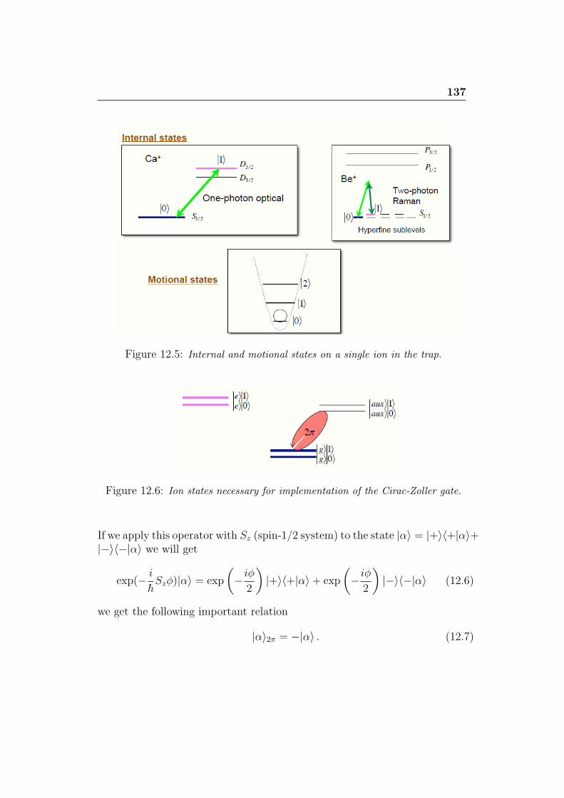
137

Figure 12.5: Internal and motional states on a single ion in the trap.

Figure 12.6: Ion states necessary for implementation of the Cirac-Zoller gate.

If we apply this operator with Sz (spin-1/2 system) to the state |α⟩ = |+⟩⟨+|α⟩+|−⟩⟨−|α⟩ we will get

exp(− i

hSzϕ)|α⟩ = exp

(−iϕ

2

)|+⟩⟨+|α⟩+ exp

(−iϕ

2

)|−⟩⟨−|α⟩ (12.6)

we get the following important relation

|α⟩2π = −|α⟩ . (12.7)

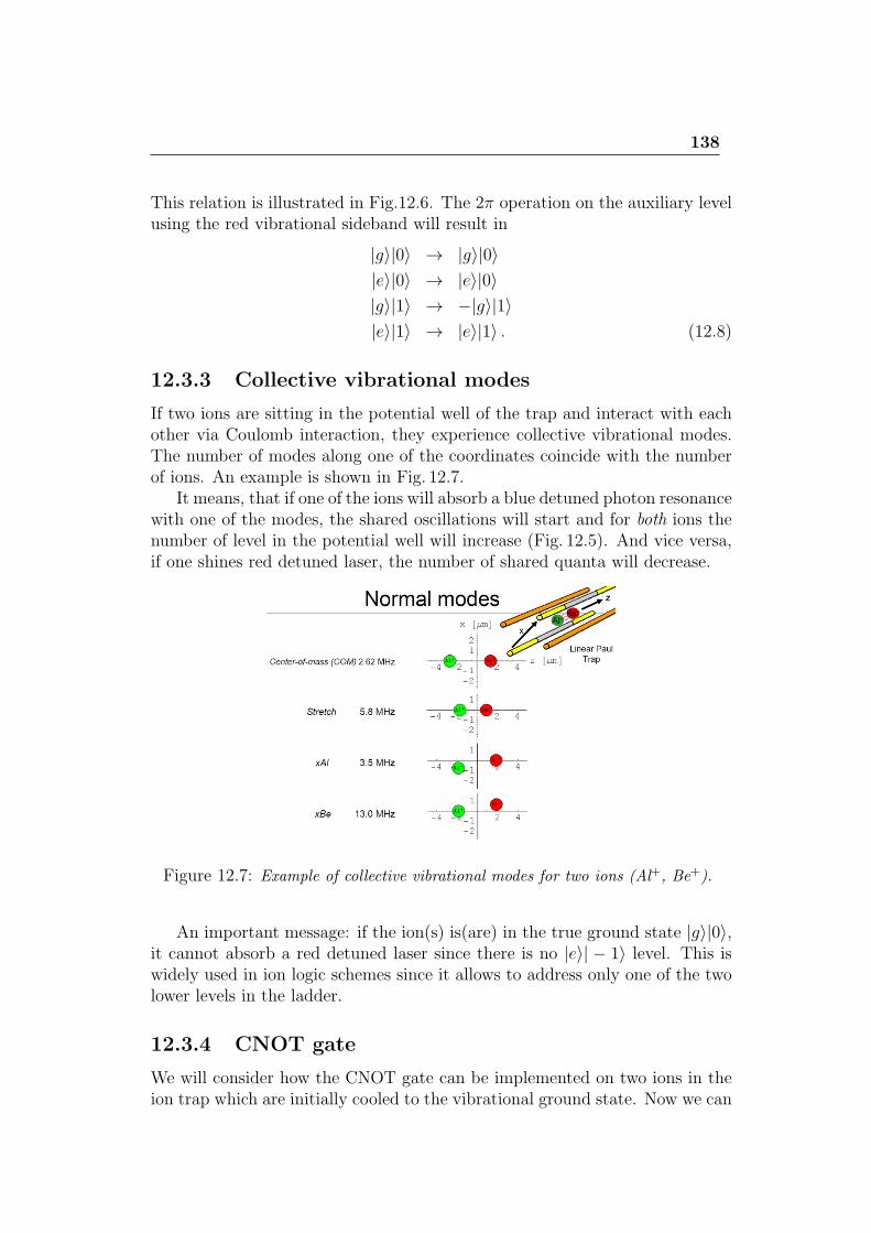
138

This relation is illustrated in Fig.12.6. The 2π operation on the auxiliary levelusing the red vibrational sideband will result in

|g⟩|0⟩ → |g⟩|0⟩|e⟩|0⟩ → |e⟩|0⟩|g⟩|1⟩ → −|g⟩|1⟩|e⟩|1⟩ → |e⟩|1⟩ . (12.8)

12.3.3 Collective vibrational modes

If two ions are sitting in the potential well of the trap and interact with eachother via Coulomb interaction, they experience collective vibrational modes.The number of modes along one of the coordinates coincide with the numberof ions. An example is shown in Fig. 12.7.

It means, that if one of the ions will absorb a blue detuned photon resonancewith one of the modes, the shared oscillations will start and for both ions thenumber of level in the potential well will increase (Fig. 12.5). And vice versa,if one shines red detuned laser, the number of shared quanta will decrease.

Figure 12.7: Example of collective vibrational modes for two ions (Al+, Be+).

An important message: if the ion(s) is(are) in the true ground state |g⟩|0⟩,it cannot absorb a red detuned laser since there is no |e⟩| − 1⟩ level. This iswidely used in ion logic schemes since it allows to address only one of the twolower levels in the ladder.

12.3.4 CNOT gate

We will consider how the CNOT gate can be implemented on two ions in theion trap which are initially cooled to the vibrational ground state. Now we can

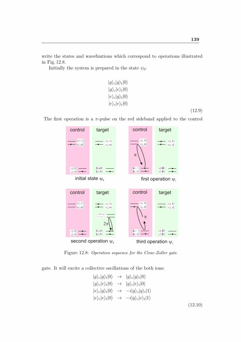
139

write the states and wavefuntions which correspond to operations illustratedin Fig. 12.8.

Initially the system is prepared in the state ψ0:

|g⟩c|g⟩t|0⟩|g⟩c|e⟩t|0⟩|e⟩c|g⟩t|0⟩|e⟩c|e⟩t|0⟩

(12.9)

The first operation is a π-pulse on the red sideband applied to the control

Figure 12.8: Operation sequence for the Cirac-Zoller gate.

gate. It will excite a collective oscillations of the both ions:

|g⟩c|g⟩t|0⟩ → |g⟩c|g⟩t|0⟩|g⟩c|e⟩t|0⟩ → |g⟩c|e⟩t|0⟩|e⟩c|g⟩t|0⟩ → −i|g⟩c|g⟩t|1⟩|e⟩c|e⟩t|0⟩ → −i|q⟩c|e⟩t|1⟩

(12.10)

140

Additionally, it will transfer population from the excited state of the controlion to its ground state with the corresponding phase which can be calculatedfrom (12.5).

The second operation is the 2π-pulse on the target ion which will changethe phase of the particular state |g⟩t|1⟩:

|g⟩c|g⟩t|0⟩ → |g⟩c|g⟩t|0⟩|g⟩c|e⟩t|0⟩ → |g⟩c|e⟩t|0⟩

−i|g⟩c|g⟩t|1⟩ → +i|g⟩c|g⟩t|1⟩−i|q⟩c|e⟩t|1⟩ → −i|q⟩c|e⟩t|1⟩

(12.11)

The last operation is again the π-pulse on the red sideband applied to thecontrol ion:

|g⟩c|g⟩t|0⟩ → |g⟩c|g⟩t|0⟩|g⟩c|e⟩t|0⟩ → |g⟩c|e⟩t|0⟩

+i|g⟩c|g⟩t|1⟩ → |e⟩c|g⟩t|0⟩−i|q⟩c|e⟩t|1⟩ → −|e⟩c|e⟩t|0⟩

(12.12)

We see that the system is returned back to the initial state ψ0 for all statesexcept the last one which changed the sign.

As we see from (12.3) it corresponds to the phase gate which can be con-verted to CNOT gate by two simple Hagamard operations (12.4).

12.4 Information transfer between clock and

cooling ions. Precision spectroscopy us-

ing quantum logic.

One of the most successful implementation of quantum logic algorithms inpractice is the recent demonstration of reading the clock transition in Al+ ionwith the help of an auxiliary sparring ion Be+. Aluminum ion has very narrowand attractive clock transition at 267 nm. One of the most important advan-tages is that this transition is barely perturbed by the black body radiation.

The problem with Al+ ion is that its strong cooling transition is at 167 nmwhich cannot be excited with modern lasers. It means that the electron shelv-ing scheme cannot be implemented here ( see Fig. 12.1). The problem of coolingcan be overcome by implementation of the sparring ion (e.g. Be+), but howthen to read the information that the clock transition is exited?

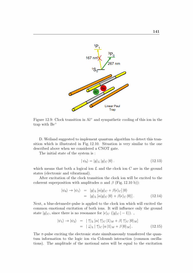
141

Figure 12.9: Clock transition in Al+ and sympathetic cooling of this ion in thetrap with Be+

D. Weiland suggested to implement quantum algorithm to detect this tran-sition which is illustrated in Fig. 12.10. Situation is very similar to the onedescribed above when we considered a CNOT gate.

The initial state of the system is :

|ψ0⟩ = |g⟩L |g⟩C |0⟩ . (12.13)

which means that both a logical ion L and the clock ion C are in the groundstates (electronic and vibrational).

After excitation of the clock transition the clock ion will be excited to thecoherent superposition with amplitudes α and β (Fig. 12.10 b)):

|ψ0⟩ → |ψ1⟩ = |g⟩L [α|g⟩C + β|e⟩C ] |0⟩= |g⟩L [α|g⟩C |0⟩+ β|e⟩C |0⟩] . (12.14)

Next, a blue-detunedπ-pulse is applied to the clock ion which will excited thecommon emotional excitation of both ions. It will influence only the groundstate |g⟩C , since there is no resonance for |e⟩C (|g⟩C | − 1⟩). ,

|ψ1⟩ → |ψ2⟩ = | ↑⟩L [α| ↑⟩C |1⟩M + β| ↑⟩C |0⟩M ]

= | ↓⟩L | ↑⟩C [α |1⟩M + β |0⟩M ] . (12.15)

The π-pulse exciting the electronic state simultaneously transferred the quan-tum information to the logic ion via Coloumb interaction (common oscilla-tions). The amplitude of the motional sates will be equal to the excitation

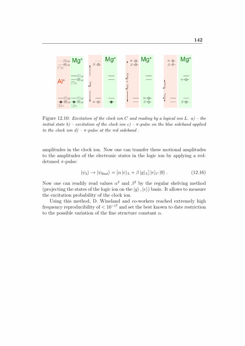
142

Figure 12.10: Excitation of the clock ion C and reading by a logical ion L. a) – the

initial state b) – excitation of the clock ion c) – π-pulse on the blue sideband applied

to the clock ion d) – π-pulse at the red sideband .

amplitudes in the clock ion. Now one can transfer these motional amplitudesto the amplitudes of the electronic states in the logic ion by applying a red-detuned π-pulse:

|ψ2⟩ → |ψfinal⟩ = [α |e⟩L + β |g⟩L] |e⟩C |0⟩ . (12.16)

Now one can readily read values α2 and β2 by the regular shelving method(projecting the states of the logic ion on the |g⟩ , |e⟩) basis. It allows to measurethe excitation probability of the clock ion.

Using this method, D. Wineland and co-workers reached extremely highfrequency reproducibility of < 10−17 and set the best known to date restrictionto the possible variation of the fine structure constant α.

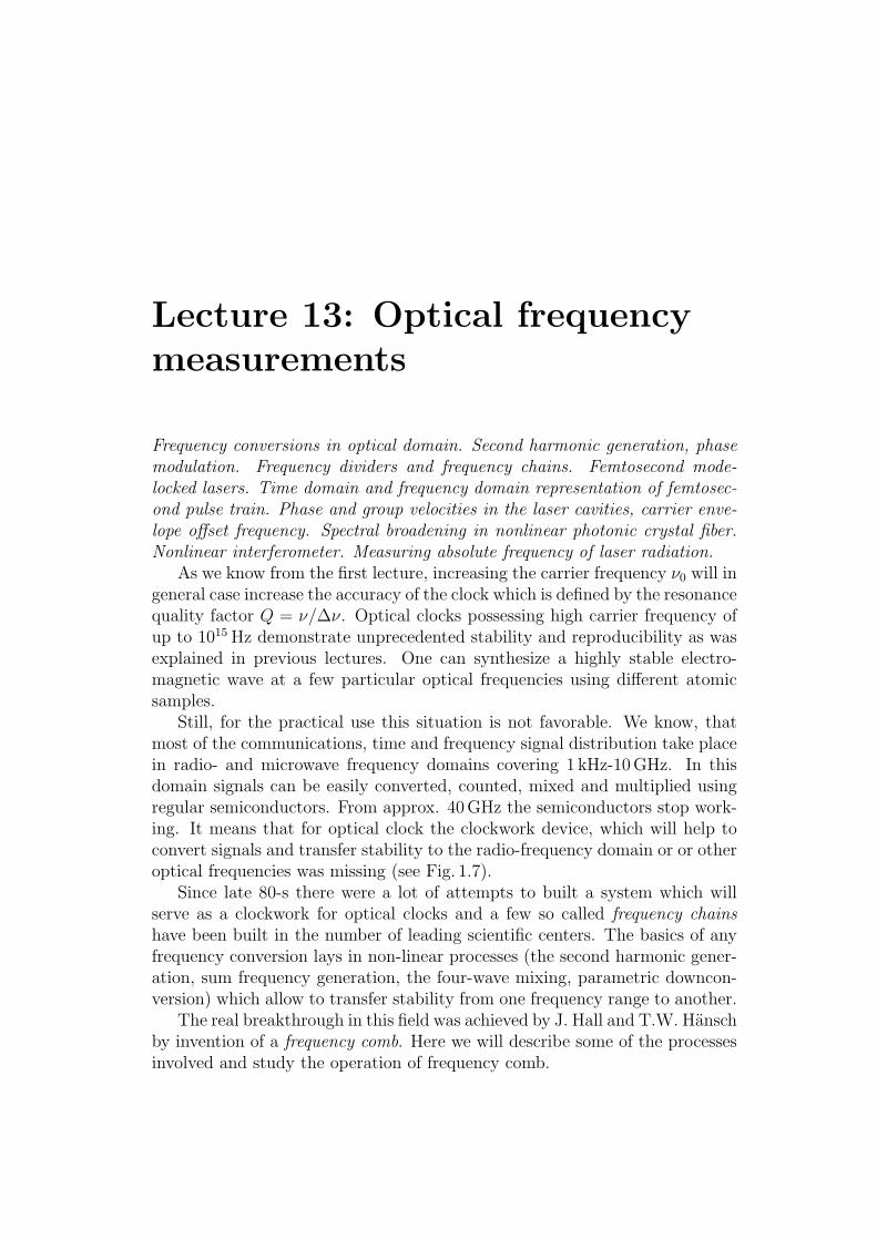
Lecture 13: Optical frequencymeasurements

Frequency conversions in optical domain. Second harmonic generation, phasemodulation. Frequency dividers and frequency chains. Femtosecond mode-locked lasers. Time domain and frequency domain representation of femtosec-ond pulse train. Phase and group velocities in the laser cavities, carrier enve-lope offset frequency. Spectral broadening in nonlinear photonic crystal fiber.Nonlinear interferometer. Measuring absolute frequency of laser radiation.

As we know from the first lecture, increasing the carrier frequency ν0 will ingeneral case increase the accuracy of the clock which is defined by the resonancequality factor Q = ν/∆ν. Optical clocks possessing high carrier frequency ofup to 1015Hz demonstrate unprecedented stability and reproducibility as wasexplained in previous lectures. One can synthesize a highly stable electro-magnetic wave at a few particular optical frequencies using different atomicsamples.

Still, for the practical use this situation is not favorable. We know, thatmost of the communications, time and frequency signal distribution take placein radio- and microwave frequency domains covering 1 kHz-10GHz. In thisdomain signals can be easily converted, counted, mixed and multiplied usingregular semiconductors. From approx. 40GHz the semiconductors stop work-ing. It means that for optical clock the clockwork device, which will help toconvert signals and transfer stability to the radio-frequency domain or or otheroptical frequencies was missing (see Fig. 1.7).

Since late 80-s there were a lot of attempts to built a system which willserve as a clockwork for optical clocks and a few so called frequency chainshave been built in the number of leading scientific centers. The basics of anyfrequency conversion lays in non-linear processes (the second harmonic gener-ation, sum frequency generation, the four-wave mixing, parametric downcon-version) which allow to transfer stability from one frequency range to another.

The real breakthrough in this field was achieved by J. Hall and T.W. Hanschby invention of a frequency comb. Here we will describe some of the processesinvolved and study the operation of frequency comb.

144

13.1 Introduction to some optical non-linear

processes

Non-linearities in the optical domain are very weak and strong fields are nec-essary to reach strong effects. Non linear processes result from non-linearmedium response — its polarization P (E). In linear approximation P ∝ E.In the general case P (E) is the non-linear function and can be written as powerseries of E

P (E) = ϵ0[χ(1)E + χ(2)E2 + χ(3)E3 + · · ·

]. (13.1)

Here χ(i) are the non-linear susceptibility coefficients which are responsible forthe process of the ith order. The square contribution in (??) is the tensor

Pi = ϵ0

3∑j,k=1

χ(2)i,j,kEjEk i, j, k = 1, 2, 3 . (13.2)

If two waves with amplitudes E1 and E2 are superimposed the result is

(E1 + E2)2 = E2

01 cos2 ω1t+ 2E01E02 cosω1t cosω2t+ E2

02 cos2 ω2t

=E2

01

2(1− cos 2ω1t) +

E202

2(1− cos 2ω2t)

+ E01E02[cos(ω2 − ω1)t− cos(ω2 + ω1)t] , (13.3)

where the terms with doubled frequencies, sum and differential frequenciesappear.

The expression (13.3) presents three types of non-linear processes. One cantreat this equation as if two photons with the frequencies ω1 and ω2 disappear,and one photon with the frequency ω3 appear. If ω1 = ω2, the process is calledsecond harmonic generation. If the frequencies are not equal it is called sumfrequency generation.

If one reads (13.3), one photon ω3 will born two photons which is calledoptical parametric generation.

The third process is optical heterodyning when the photon ω1 −ω2 is born.To satisfy the energy conservation law two other photons should appear: ω1+ω2 = ω1 + (−ω2 + ω2) + ω2 = (ω1 − ω2) + 2ω2 .

The four wave mixing involves three photons and is described by the cubicterm in (13.1). If the condition of phase synchronism is fulfilled, three photonswith frequencies ω1, ω2, ω3 will be converted to other frequencies. An importantcombination for this discussion is ω4 = ω1 + ω2 − ω3.

Please note, that due to parity and momentum conservation reasons thetwo-photon processes may take place only with anisotropic media (some crys-tals), while in anisotropic materials (glass, gas, liquid) they are very inefficient.On the other hand, the three-photon process does not have this restriction andcan take place in isotropic media as well.

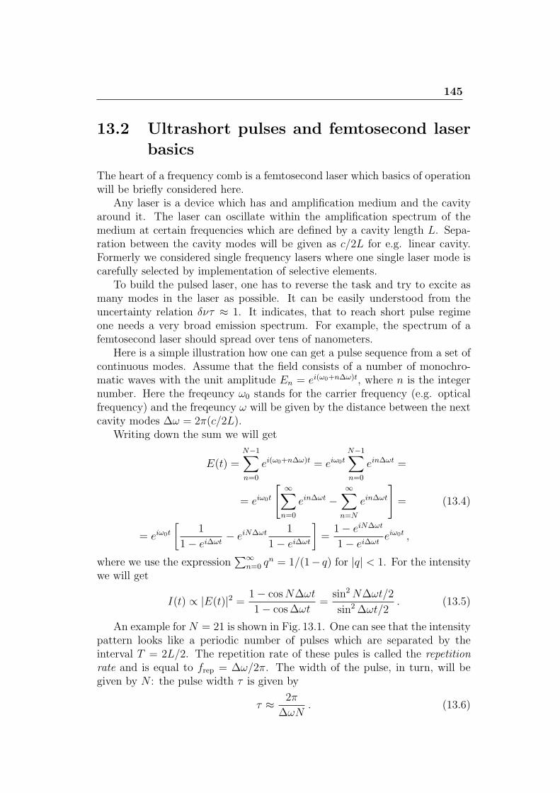
145

13.2 Ultrashort pulses and femtosecond laser

basics

The heart of a frequency comb is a femtosecond laser which basics of operationwill be briefly considered here.

Any laser is a device which has and amplification medium and the cavityaround it. The laser can oscillate within the amplification spectrum of themedium at certain frequencies which are defined by a cavity length L. Sepa-ration between the cavity modes will be given as c/2L for e.g. linear cavity.Formerly we considered single frequency lasers where one single laser mode iscarefully selected by implementation of selective elements.

To build the pulsed laser, one has to reverse the task and try to excite asmany modes in the laser as possible. It can be easily understood from theuncertainty relation δντ ≈ 1. It indicates, that to reach short pulse regimeone needs a very broad emission spectrum. For example, the spectrum of afemtosecond laser should spread over tens of nanometers.

Here is a simple illustration how one can get a pulse sequence from a set ofcontinuous modes. Assume that the field consists of a number of monochro-matic waves with the unit amplitude En = ei(ω0+n∆ω)t, where n is the integernumber. Here the freqeuncy ω0 stands for the carrier frequency (e.g. opticalfrequency) and the freqeuncy ω will be given by the distance between the nextcavity modes ∆ω = 2π(c/2L).

Writing down the sum we will get

E(t) =N−1∑n=0

ei(ω0+n∆ω)t = eiω0t

N−1∑n=0

ein∆ωt =

= eiω0t

[∞∑n=0

ein∆ωt −∞∑

n=N

ein∆ωt

]= (13.4)

= eiω0t

[1

1− ei∆ωt− eiN∆ωt 1

1− ei∆ωt

]=

1− eiN∆ωt

1− ei∆ωteiω0t ,

where we use the expression∑∞

n=0 qn = 1/(1− q) for |q| < 1. For the intensity

we will get

I(t) ∝ |E(t)|2 = 1− cosN∆ωt

1− cos∆ωt=

sin2N∆ωt/2

sin2∆ωt/2. (13.5)

An example for N = 21 is shown in Fig. 13.1. One can see that the intensitypattern looks like a periodic number of pulses which are separated by theinterval T = 2L/2. The repetition rate of these pules is called the repetitionrate and is equal to frep = ∆ω/2π. The width of the pulse, in turn, will begiven by N : the pulse width τ is given by

τ ≈ 2π

∆ωN. (13.6)

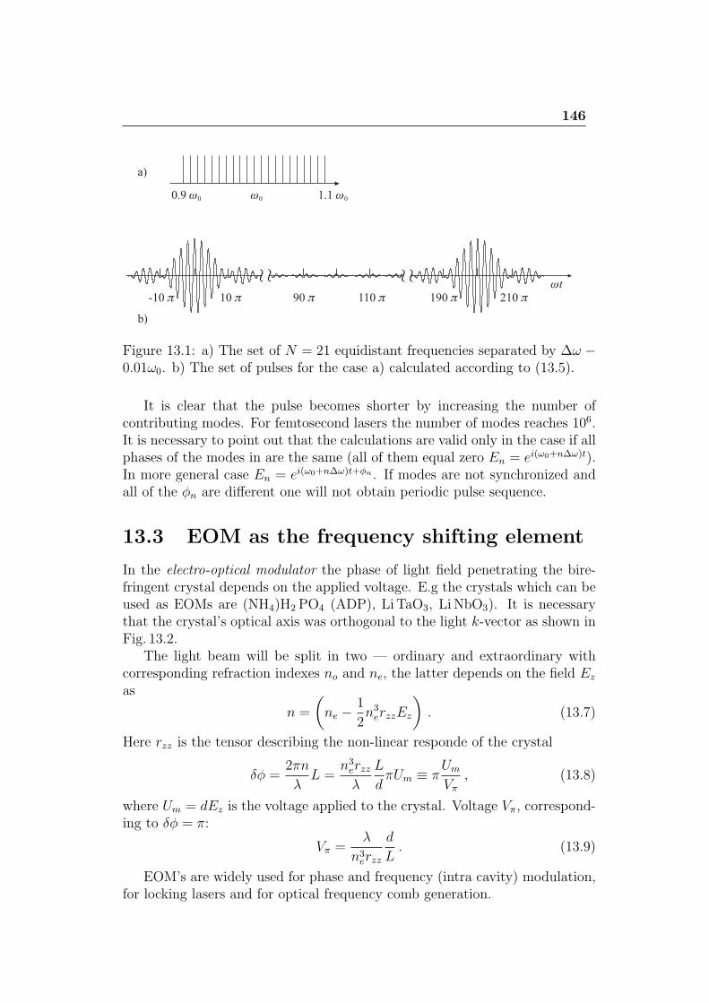
146

Figure 13.1: a) The set of N = 21 equidistant frequencies separated by ∆ω −0.01ω0. b) The set of pulses for the case a) calculated according to (13.5).

It is clear that the pulse becomes shorter by increasing the number ofcontributing modes. For femtosecond lasers the number of modes reaches 106.It is necessary to point out that the calculations are valid only in the case if allphases of the modes in are the same (all of them equal zero En = ei(ω0+n∆ω)t).In more general case En = ei(ω0+n∆ω)t+ϕn . If modes are not synchronized andall of the ϕn are different one will not obtain periodic pulse sequence.

13.3 EOM as the frequency shifting element

In the electro-optical modulator the phase of light field penetrating the bire-fringent crystal depends on the applied voltage. E.g the crystals which can beused as EOMs are (NH4)H2 PO4 (ADP), LiTaO3, Li NbO3). It is necessarythat the crystal’s optical axis was orthogonal to the light k-vector as shown inFig. 13.2.

The light beam will be split in two — ordinary and extraordinary withcorresponding refraction indexes no and ne, the latter depends on the field Ez

as

n =

(ne −

1

2n3erzzEz

). (13.7)

Here rzz is the tensor describing the non-linear responde of the crystal

δϕ =2πn

λL =

n3erzzλ

L

dπUm ≡ π

Um

Vπ, (13.8)

where Um = dEz is the voltage applied to the crystal. Voltage Vπ, correspond-ing to δϕ = π:

Vπ =λ

n3erzz

d

L. (13.9)

EOM’s are widely used for phase and frequency (intra cavity) modulation,for locking lasers and for optical frequency comb generation.

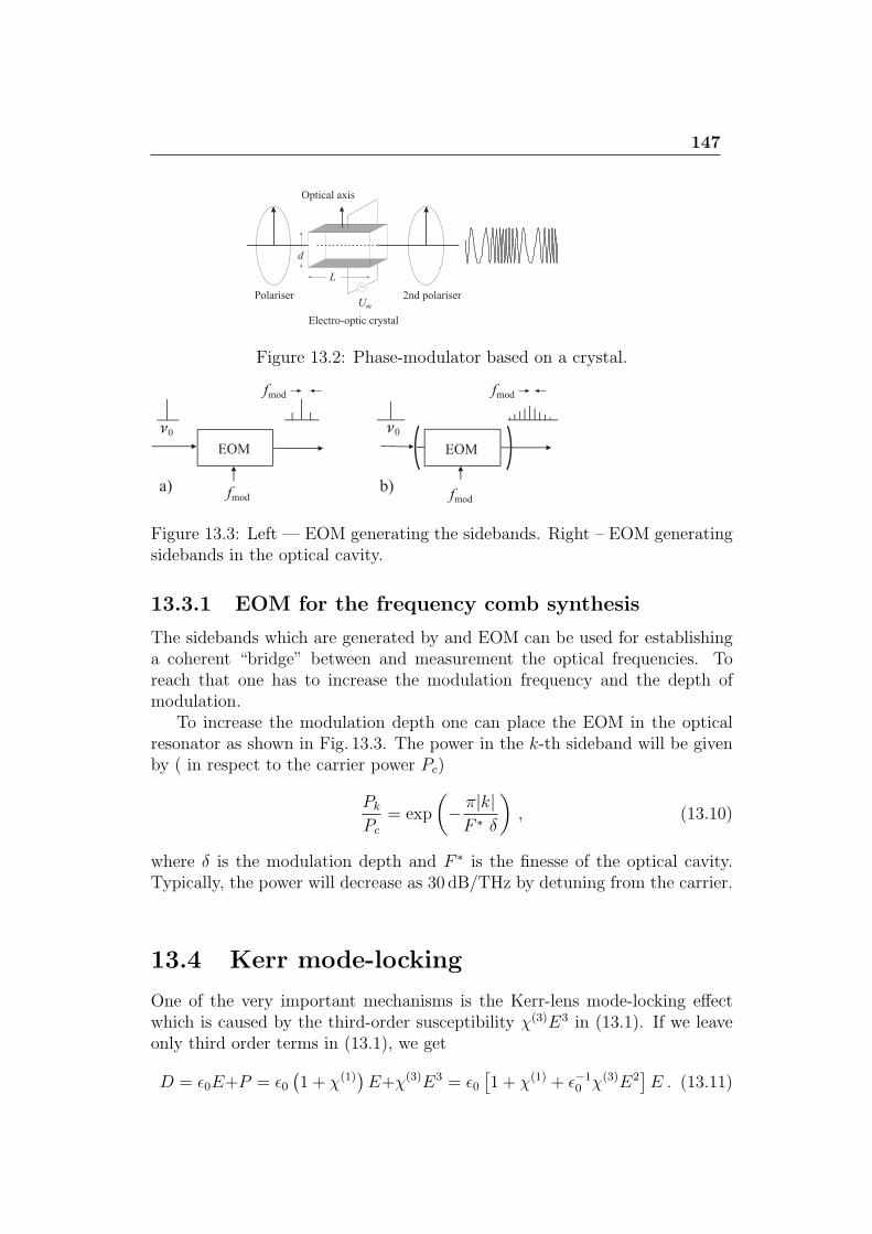
147

Figure 13.2: Phase-modulator based on a crystal.

Figure 13.3: Left — EOM generating the sidebands. Right – EOM generatingsidebands in the optical cavity.

13.3.1 EOM for the frequency comb synthesis

The sidebands which are generated by and EOM can be used for establishinga coherent “bridge” between and measurement the optical frequencies. Toreach that one has to increase the modulation frequency and the depth ofmodulation.

To increase the modulation depth one can place the EOM in the opticalresonator as shown in Fig. 13.3. The power in the k-th sideband will be givenby ( in respect to the carrier power Pc)

Pk

Pc

= exp

(− π|k|F ∗ δ

), (13.10)

where δ is the modulation depth and F ∗ is the finesse of the optical cavity.Typically, the power will decrease as 30 dB/THz by detuning from the carrier.

13.4 Kerr mode-locking

One of the very important mechanisms is the Kerr-lens mode-locking effectwhich is caused by the third-order susceptibility χ(3)E3 in (13.1). If we leaveonly third order terms in (13.1), we get

D = ϵ0E+P = ϵ0(1 + χ(1)

)E+χ(3)E3 = ϵ0

[1 + χ(1) + ϵ−1

0 χ(3)E2]E . (13.11)

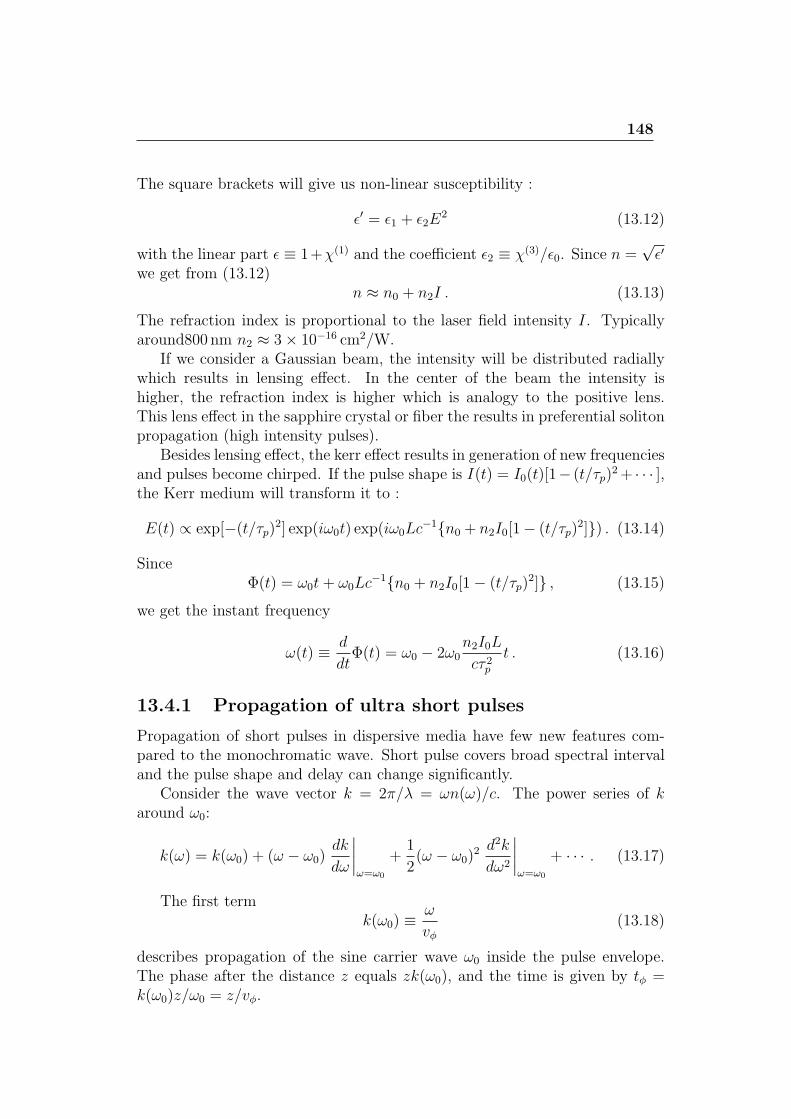
148

The square brackets will give us non-linear susceptibility :

ϵ′ = ϵ1 + ϵ2E2 (13.12)

with the linear part ϵ ≡ 1+χ(1) and the coefficient ϵ2 ≡ χ(3)/ϵ0. Since n =√ϵ′

we get from (13.12)n ≈ n0 + n2I . (13.13)

The refraction index is proportional to the laser field intensity I. Typicallyaround800 nm n2 ≈ 3× 10−16 cm2/W.

If we consider a Gaussian beam, the intensity will be distributed radiallywhich results in lensing effect. In the center of the beam the intensity ishigher, the refraction index is higher which is analogy to the positive lens.This lens effect in the sapphire crystal or fiber the results in preferential solitonpropagation (high intensity pulses).

Besides lensing effect, the kerr effect results in generation of new frequenciesand pulses become chirped. If the pulse shape is I(t) = I0(t)[1− (t/τp)

2+ · · · ],the Kerr medium will transform it to :

E(t) ∝ exp[−(t/τp)2] exp(iω0t) exp(iω0Lc

−1n0 + n2I0[1− (t/τp)2]) . (13.14)

SinceΦ(t) = ω0t+ ω0Lc

−1n0 + n2I0[1− (t/τp)2] , (13.15)

we get the instant frequency

ω(t) ≡ d

dtΦ(t) = ω0 − 2ω0

n2I0L

cτ 2pt . (13.16)

13.4.1 Propagation of ultra short pulses

Propagation of short pulses in dispersive media have few new features com-pared to the monochromatic wave. Short pulse covers broad spectral intervaland the pulse shape and delay can change significantly.

Consider the wave vector k = 2π/λ = ωn(ω)/c. The power series of karound ω0:

k(ω) = k(ω0) + (ω − ω0)dk

dω

∣∣∣∣ω=ω0

+1

2(ω − ω0)

2 d2k

dω2

∣∣∣∣ω=ω0

+ · · · . (13.17)

The first termk(ω0) ≡

ω

vϕ(13.18)

describes propagation of the sine carrier wave ω0 inside the pulse envelope.The phase after the distance z equals zk(ω0), and the time is given by tϕ =k(ω0)z/ω0 = z/vϕ.

149

The second termdk

dω

∣∣∣∣ω=ω0

=1

υg(13.19)

gives the propagation of the envelope of the pulse vg . The correspondingrefraction index equals

ng(λ) ≡c

vg= c

dk

dω= c

d

dω

ω n

c= n+ ω

dn

dω= n(λ)− λ

d

dλn(λ) , (13.20)

where we used dω/dλ = −ω/λ.The third term in (13.17) is so-called group velocity dispersion

d2k

dω2

∣∣∣∣ω=ω0

=d

dω

1

υg(ω)

∣∣∣∣ω=ω0

. (13.21)

The pulse shape changes after propagating in the medium. It is typical char-acterized by the parameter

D ≡ 1

L

dT

dλ, (13.22)

where λ is the wavelength in vacuum, T is the propagation time for the pulsealong the length L in the medium. Since T = L/vg

D =d 1vg

dλ= −ω

λ

d 1vg

dλ= −2πc

λ2d2k

dω2, (13.23)

In the optical fibers the dispersion of the group velocity is caused also by thewaveguide dispersion.

13.5 Precision optical spectroscopy and opti-

cal frequency measurements

The principle of modern optical frequency measurement is presented in fig. 13.4.A laser is tuned to the wavelength of a narrow metrological transition (usuallyreferred to as a “clock transition”) in an atomic, ionic or molecular sample.Most commonly, the laser frequency is stabilized by active feedback to a trans-mission peak of a well isolated optical cavity (“reference cavity”) which allowsto achieve sub-hertz spectral line width of the interrogating laser. Some recentadvances in laser stabilization technique will be described in section ??. Thelaser frequency is then scanned across the transition which allows to find theline center ω0 using an appropriate line shape model. The measured transi-tion quality factor can reach 1015 which provides extremely high resolution.To obtain the transition frequency the beat note ωbeat between the laser andone of the modes of the stabilized frequency comb is measured with the help

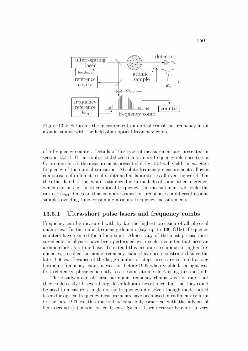
150

Figure 13.4: Setup for the measurement an optical transition frequency in anatomic sample with the help of an optical frequency comb.

of a frequency counter. Details of this type of measurement are presented insection 13.5.1. If the comb is stabilized to a primary frequency reference (i.e. aCs atomic clock), the measurement presented in fig. 13.4 will yield the absolutefrequency of the optical transition. Absolute frequency measurements allow acomparison of different results obtained at laboratories all over the world. Onthe other hand, if the comb is stabilized with the help of some other reference,which can be e.g. another optical frequency, the measurement will yield theratio ω0/ωref . One can thus compare transition frequencies in different atomicsamples avoiding time-consuming absolute frequency measurements.

13.5.1 Ultra-short pulse lasers and frequency combs

Frequency can be measured with by far the highest precision of all physicalquantities. In the radio frequency domain (say up to 100 GHz), frequencycounters have existed for a long time. Almost any of the most precise mea-surements in physics have been performed with such a counter that uses anatomic clock as a time base. To extend this accurate technique to higher fre-quencies, so called harmonic frequency chains have been constructed since thelate 1960ies. Because of the large number of steps necessary to build a longharmonic frequency chain, it was not before 1995 when visible laser light wasfirst referenced phase coherently to a cesium atomic clock using this method.

The disadvantage of these harmonic frequency chains was not only thatthey could easily fill several large laser laboratories at once, but that they couldbe used to measure a single optical frequency only. Even though mode lockedlasers for optical frequency measurements have been used in rudimentary formin the late 1970ies, this method became only practical with the advent offemtosecond (fs) mode locked lasers. Such a laser necessarily emits a very

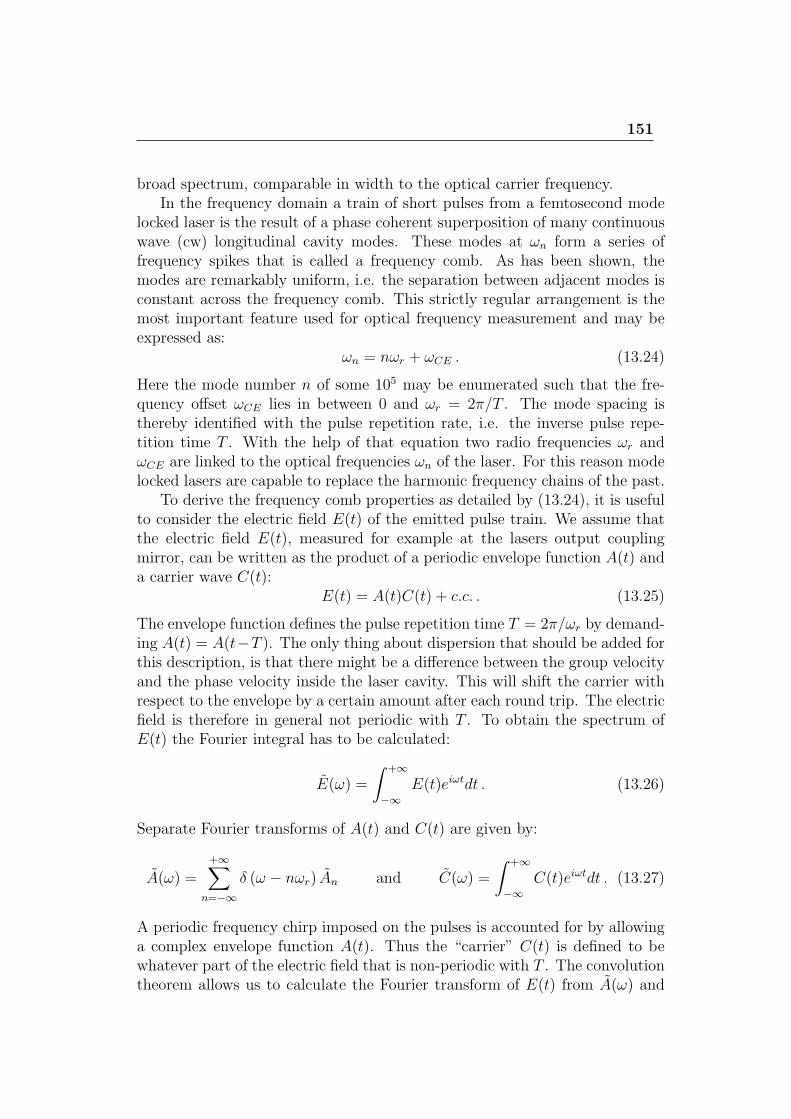
151

broad spectrum, comparable in width to the optical carrier frequency.In the frequency domain a train of short pulses from a femtosecond mode

locked laser is the result of a phase coherent superposition of many continuouswave (cw) longitudinal cavity modes. These modes at ωn form a series offrequency spikes that is called a frequency comb. As has been shown, themodes are remarkably uniform, i.e. the separation between adjacent modes isconstant across the frequency comb. This strictly regular arrangement is themost important feature used for optical frequency measurement and may beexpressed as:

ωn = nωr + ωCE . (13.24)

Here the mode number n of some 105 may be enumerated such that the fre-quency offset ωCE lies in between 0 and ωr = 2π/T . The mode spacing isthereby identified with the pulse repetition rate, i.e. the inverse pulse repe-tition time T . With the help of that equation two radio frequencies ωr andωCE are linked to the optical frequencies ωn of the laser. For this reason modelocked lasers are capable to replace the harmonic frequency chains of the past.

To derive the frequency comb properties as detailed by (13.24), it is usefulto consider the electric field E(t) of the emitted pulse train. We assume thatthe electric field E(t), measured for example at the lasers output couplingmirror, can be written as the product of a periodic envelope function A(t) anda carrier wave C(t):

E(t) = A(t)C(t) + c.c. . (13.25)

The envelope function defines the pulse repetition time T = 2π/ωr by demand-ing A(t) = A(t−T ). The only thing about dispersion that should be added forthis description, is that there might be a difference between the group velocityand the phase velocity inside the laser cavity. This will shift the carrier withrespect to the envelope by a certain amount after each round trip. The electricfield is therefore in general not periodic with T . To obtain the spectrum ofE(t) the Fourier integral has to be calculated:

E(ω) =

∫ +∞

−∞E(t)eiωtdt . (13.26)

Separate Fourier transforms of A(t) and C(t) are given by:

A(ω) =+∞∑

n=−∞

δ (ω − nωr) An and C(ω) =

∫ +∞

−∞C(t)eiωtdt . (13.27)

A periodic frequency chirp imposed on the pulses is accounted for by allowinga complex envelope function A(t). Thus the “carrier” C(t) is defined to bewhatever part of the electric field that is non-periodic with T . The convolutiontheorem allows us to calculate the Fourier transform of E(t) from A(ω) and

152

C(ω):

E(ω) =1

2π

∫ +∞

−∞A(ω′)C(ω − ω′)dω′ + c.c. =

1

2π

+∞∑n=−∞

AnC (ω − nωr) + c.c. .

(13.28)The sum represents a periodic spectrum in frequency space. If the spectral

width of the carrier wave ∆ωc is much smaller than the mode separation ωr,it represents a regularly spaced comb of laser modes just like (13.24), withidentical spectral line shapes. If C(ω) is centered at say ωc, then the comb isshifted by ωc from containing only exact harmonics of ωr. The frequencies ofthe mode members are calculated from the mode number n:

ωn = nωr + ωc . (13.29)

The measurement of the ωc as described below usually yields a value moduloωr, so that renumbering the modes will restrict the offset frequency to smallervalues than the repetition frequency and (13.24) and (13.29) are identical.

If the carrier wave is monochromatic C(t) = e−iωct−iφ, its spectrum willbe δ-shaped and centered at the carrier frequency ωc. The individual modesare also δ-functions C(ω) = δ(ω − ωc)e

−iφ. The frequency offset (13.29) isidentified with the carrier frequency. According to (13.25) each round tripwill shift the carrier wave with respect to the envelope by ∆φ = arg(C(t −T )) − arg(C(t)) = ωcT so that the frequency offset may also be identified byωCE = ∆φ/T . In a typical laser cavity this pulse-to-pulse carrier-envelopephase shift is much larger than 2π, but measurements usually yield a valuemodulo 2π. The restriction 0 ≤ ∆φ ≤ 2π is synonymous with the restriction0 ≤ ωCE ≤ ωr introduced above. Figure 13.5 sketches this situation in thetime domain for a chirp free pulse train.

Extending the frequency comb

The spectral width of a pulse train emitted by a fs laser can be significantlybroadened in a single mode fiber by self phase modulation. Assuming a singlemode carrier wave, a pulse that has propagated the length L acquires a selfinduced phase shift of

ΦNL(t) = −n2I(t)ωcL/c , (13.30)

where the pulse intensity is given by I(t) = 12cε0|A(t)|2. For fused silica the

non-linear Kerr coefficient n2 is comparatively small but almost instantaneouseven on the time scale of fs pulses. This means that different parts of thepulse travel at different speed. The result is a frequency chirp across the pulsewithout affecting its duration. The pulse is no longer at the Fourier limit sothat the spectrum is much broader than the inverse pulse duration where the

153

Figure 13.5: Consecutive un-chirped pulses (A(t) is real) with carrier frequencyωc and the corresponding spectrum (not to scale). Because the carrier propa-gates with a different velocity within the laser cavity than the envelope (withphase- and group velocity respectively), the electric field does not repeat itselfafter one round trip. A pulse-to-pulse phase shift ∆φ results in an offset fre-quency of ωCE = ∆φ/T . The mode spacing is given by the repetition rate ωr.The width of the spectral envelope is given by the inverse pulse duration upto a factor of order unity that depends on the pulse shape.

extra frequencies are determined by the time derivative of the self inducedphase shift ΦNL(t). Therefore pure self-phase modulation would modify theenvelope function in (13.25) according to

A(t) −→ A(t)eiΦNL(t). (13.31)

Because ΦNL(t) has the same periodicity as A(t) the comb structure of thespectrum is maintained and the derivations (13.28) remain valid because pe-riodicity of A(t) was the only assumption made. An optical fiber is mostappropriate for this process because it can maintain the necessary small focusarea over a virtually unlimited length. In practice, however, other pulse re-shaping mechanism, both linear and non-linear, are present so that the aboveexplanation might be too simple.

A microstructured fiber uses an array of submicron-sized air holes thatsurround the fiber core and run the length of a silica fiber to obtain a desiredeffective dispersion. This can be used to maintain the high peak power over anextended propagation length and to significantly increase the spectral broad-ening. With these fibers it became possible to broaden low peak power, highrepetition rate lasers to beyond one optical octave as shown in fig. 13.6.

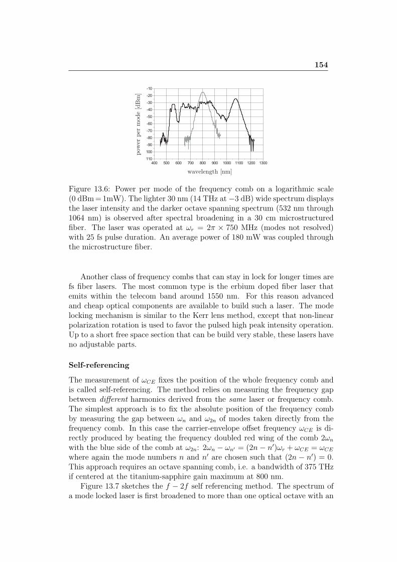
154

Figure 13.6: Power per mode of the frequency comb on a logarithmic scale(0 dBm=1mW). The lighter 30 nm (14 THz at −3 dB) wide spectrum displaysthe laser intensity and the darker octave spanning spectrum (532 nm through1064 nm) is observed after spectral broadening in a 30 cm microstructuredfiber. The laser was operated at ωr = 2π × 750 MHz (modes not resolved)with 25 fs pulse duration. An average power of 180 mW was coupled throughthe microstructure fiber.

Another class of frequency combs that can stay in lock for longer times arefs fiber lasers. The most common type is the erbium doped fiber laser thatemits within the telecom band around 1550 nm. For this reason advancedand cheap optical components are available to build such a laser. The modelocking mechanism is similar to the Kerr lens method, except that non-linearpolarization rotation is used to favor the pulsed high peak intensity operation.Up to a short free space section that can be build very stable, these lasers haveno adjustable parts.

Self-referencing

The measurement of ωCE fixes the position of the whole frequency comb andis called self-referencing. The method relies on measuring the frequency gapbetween different harmonics derived from the same laser or frequency comb.The simplest approach is to fix the absolute position of the frequency combby measuring the gap between ωn and ω2n of modes taken directly from thefrequency comb. In this case the carrier-envelope offset frequency ωCE is di-rectly produced by beating the frequency doubled red wing of the comb 2ωn

with the blue side of the comb at ω2n: 2ωn − ωn′ = (2n− n′)ωr + ωCE = ωCE

where again the mode numbers n and n′ are chosen such that (2n − n′) = 0.This approach requires an octave spanning comb, i.e. a bandwidth of 375 THzif centered at the titanium-sapphire gain maximum at 800 nm.

Figure 13.7 sketches the f − 2f self referencing method. The spectrum ofa mode locked laser is first broadened to more than one optical octave with an

155

Figure 13.7: (left) — The principle of the f − 2f self referencing relieson detecting a beat note at ωCE between the frequency doubled “red” wing2(nωr + ωCE) of the frequency comb and the “blue” modes at 2nωr + ωCE.(right) — More detailed layout of the self referencing scheme. See text fordetails.

optical fiber. A broad band λ/2 wave plate allows to choose the polarizationwith the most efficient spectral broadening. After the fiber a dichroic mirrorseparates the infrared (“red”) part from the green (“blue”). The former isfrequency doubled in a non-linear crystal and reunited with the green part tocreate a wealth of beat notes, all at ωCE. These beat notes emerge as frequencydifference between 2ωn −ω2n according to (13.24) for various values of n. Thenumber of contributing modes is given by the phase matching bandwidth ∆νpmof the doubling crystal and can easily exceed 1 THz.

As described, both degrees of freedom ωr and ωCE of the frequency combcan be measured up to a sign in ωCE that will be discussed below. For stabiliza-tion of these frequencies, say relative to a radio frequency reference, it is alsonecessary to control them. Again the repetition rate turns out to be simpler.Mounting one of the laser’s cavity mirrors on a piezo electric transducer allowsto control the pulse round trip time. Controlling the carrier envelope frequencyrequires some effort. Any laser parameter that has a different influence on thecavity round trip phase delay and the cavity round trip group delay may beused to change ωCE. Experimentally it turned out that the energy of the pulsestored inside the mode locked laser cavity has a strong influence on ωCE. Tophase lock the carrier envelope offset frequency ωCE, one can therefore controlthe laser power through its energy source (pump laser).

Frequency conversions

Given the above we conclude that the frequency comb may serve as a frequencyconverter between the optical and radio frequency domains allowing to performthe following phase coherent operations:

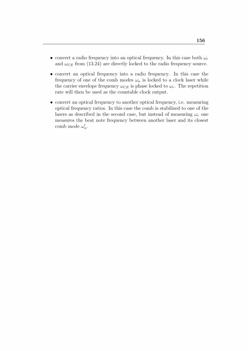
156

• convert a radio frequency into an optical frequency. In this case both ωr

and ωCE from (13.24) are directly locked to the radio frequency source.

• convert an optical frequency into a radio frequency. In this case thefrequency of one of the comb modes ωn is locked to a clock laser whilethe carrier envelope frequency ωCE is phase locked to ωr. The repetitionrate will then be used as the countable clock output.

• convert an optical frequency to another optical frequency, i.e. measuringoptical frequency ratios. In this case the comb is stabilized to one of thelasers as described in the second case, but instead of measuring ωr onemeasures the beat note frequency between another laser and its closestcomb mode ω′

n.