Embed Size (px)
Citation preview

Precision Landmark Location forMachine Vision and Photogrammetry

José A. GutierrezBrian S.R. Armstrong
Precision LandmarkLocation forMachine Vision andPhotogrammetryFinding and Achievingthe Maximum Possible Accuracy
123

José A. Gutierrez, PhDEmerson CorporationCorporate TechnologySt. LouisMissouriUSA
Brian S.R. Armstrong, PhD, P.E.Department of Electrical Engineering
and Computer ScienceUniversity of Wisconsin – MilwaukeeMilwaukeeWisconsinUSA
British Library Cataloguing in Publication DataGutierrez, Jose A.
Precision landmark location for machine vision andphotogrammetry : finding and achieving the maximum possibleaccuracy1. Computer vision 2. Photogrammetry - Digital techniquesI. Title II. Armstrong, Brian Stewart Randall006.3’7
ISBN-13: 9781846289125
Library of Congress Control Number: 2007936782
ISBN 978-1-84628-912-5 e-ISBN 978-1-84628-913-2Printed on acid-free paper
© Springer-Verlag London Limited 2008
MATLAB® is a registered trademark of The MathWorks, Inc., 3 Apple Hill Drive, Natick,MA 01760-2098, USA. http://www.mathworks.com
Apart from any fair dealing for the purposes of research or private study, or criticism orreview, as permitted under the Copyright, Designs and Patents Act 1988, this publicationmay only be reproduced, stored or transmitted, in any form or by any means, with theprior permission in writing of the publishers, or in the case of reprographic reproductionin accordance with the terms of licences issued by the Copyright Licensing Agency. En-quiries concerning reproduction outside those terms should be sent to the publishers.
The use of registered names, trademarks, etc. in this publication does not imply, even inthe absence of a specific statement, that such names are exempt from the relevant laws andregulations and therefore free for general use.
The publisher makes no representation, express or implied, with regard to the accuracy ofthe information contained in this book and cannot accept any legal responsibility or lia-bility for any errors or omissions that may be made.
9 8 7 6 5 4 3 2 1
Springer Science+Business Mediaspringer.com

To Alan Alejandro and Natacha
To Claire, Amanda, and Beatrice

Preface
Precision landmark location in digital images is one of those inter-esting problems in which industrial practice seems to outstrip theresults available in the scholarly literature. Approaching this problem,we remarked that the best-performing commercial close-range pho-togrammetry systems have specified accuracies of a part per 100,000,which translates to 10–20 millipixels of uncertainty in locating featuresfor measurement. At the same time, articles we identified in the aca-demic literature didn’t seem to give any firm answer about when thislevel of performance is possible or how it can be achieved.
We came to the problem of precision landmark location by a processthat must be familiar to many: out of a desire to calibrate an image-metrology test bench using landmarks in well-known locations. It isstraightforward to perform the calibration, minimizing errors in a leastsquares sense; but we were also interested to know what fraction of theresidual errors should be attributed to the determination of landmarklocations in the images, and whether this error source could be reduced.
To address these questions, we knew we had to go beyond the con-sideration of binary images. At the limit of sensitivity, it is clear that allof the grayscale information must be used. Likewise, we knew we hadto go beyond an idealized model of image formation that considers thepixels to be point-wise samples of the image; since we were lookingfor changes to the image that arise with landmark displacements ofa small fraction of a pixel width, the details of the photosensitive areawithin each pixel were going to play a role. Finally, rather than fo-cusing on the performance of a particular algorithm, it seemed betterto pursue the Cramér–Rao lower bound, and thereby determine analgorithm-independent answer to the question. There was, after all,a sheer curiosity to know whether part-per-100,000 accuracy is reallypossible for close-range photogrammetry with digital images.
In a convergence of necessity and opportunity, it turns out thatconsidering a richer model of the image formation process is itselfinstrumental in making the calculation of the uncertainty tractable.The smoothing introduced into the image by diffraction and othersources has been neglected in some past investigations, which have

viii Preface
idealized the digital image as point-wise samples from a discontin-uous description of the image. Far from being an unwanted compli-cation, the smoothing makes the calculations feasible. If the imagewere discontinuous, we would have been obliged to represent it witha smoothed approximation in order to calculate the Cramér–Rao lowerbound.
With the Cramér–Rao bound in hand, it is possible to determine thegap between the performance of well-known algorithms for landmarklocation and the theoretical limit, and to devise new algorithms thatperform near the limit.
In response to the question of whether part-per-100,000 measure-ment is possible from digital images, the reader is invited to turn thepage and join us in exploring the limits to precision landmark location.
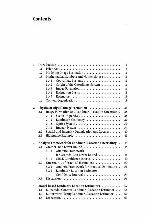
Contents
1 Introduction . . . . . . . . . . . . . . . . . . . . . . . . . . . . . . . . . . . . . . . . . . 11.1 Prior Art . . . . . . . . . . . . . . . . . . . . . . . . . . . . . . . . . . . . . . . . . 51.2 Modeling Image Formation . . . . . . . . . . . . . . . . . . . . . . . . . 111.3 Mathematical Symbols and Nomenclature . . . . . . . . . . . . 15
1.3.1 Coordinate Systems . . . . . . . . . . . . . . . . . . . . . . . . . 151.3.2 Origin of the Coordinate System . . . . . . . . . . . . . . 161.3.3 Image Formation . . . . . . . . . . . . . . . . . . . . . . . . . . . 161.3.4 Estimation Basics . . . . . . . . . . . . . . . . . . . . . . . . . . . 181.3.5 Estimators . . . . . . . . . . . . . . . . . . . . . . . . . . . . . . . . . 19
1.4 Content Organization . . . . . . . . . . . . . . . . . . . . . . . . . . . . . . 19
2 Physics of Digital Image Formation . . . . . . . . . . . . . . . . . . . . . . 212.1 Image Formation and Landmark Location Uncertainty . 28
2.1.1 Scene Properties . . . . . . . . . . . . . . . . . . . . . . . . . . . . 282.1.2 Landmark Geometry . . . . . . . . . . . . . . . . . . . . . . . . 292.1.3 Optics System . . . . . . . . . . . . . . . . . . . . . . . . . . . . . . 302.1.4 Imager System . . . . . . . . . . . . . . . . . . . . . . . . . . . . . 34
2.2 Spatial and Intensity Quantization and Locales . . . . . . . . 402.3 Illustrative Example . . . . . . . . . . . . . . . . . . . . . . . . . . . . . . . 43
3 Analytic Framework for Landmark Location Uncertainty . . . 453.1 Cramér–Rao Lower Bound . . . . . . . . . . . . . . . . . . . . . . . . . 45
3.1.1 Analytic Frameworkfor Cramér–Rao Lower Bound . . . . . . . . . . . . . . . . 46
3.1.2 CRLB Confidence Interval . . . . . . . . . . . . . . . . . . . 493.2 Uncertainty of Practical Estimators . . . . . . . . . . . . . . . . . . 50
3.2.1 Analytic Framework for Practical Estimators . . . 513.2.2 Landmark Location Estimator
Confidence Interval . . . . . . . . . . . . . . . . . . . . . . . . . 543.3 Discussion . . . . . . . . . . . . . . . . . . . . . . . . . . . . . . . . . . . . . . . 56
4 Model-based Landmark Location Estimators . . . . . . . . . . . . . . 574.1 Ellipsoidal Contour Landmark Location Estimator . . . . 584.2 Butterworth Tepuy Landmark Location Estimator . . . . . 604.3 Discussion . . . . . . . . . . . . . . . . . . . . . . . . . . . . . . . . . . . . . . . 63

x Contents
5 Two-dimensional Noncollocated Numerical Integration . . . . 655.1 Noncollocated Simpson Rule: 1-D . . . . . . . . . . . . . . . . . . . 665.2 Noncollocated Simpson Rule: 2-D . . . . . . . . . . . . . . . . . . . 70
6 Computational Tools . . . . . . . . . . . . . . . . . . . . . . . . . . . . . . . . . . . 796.1 EyeEntity . . . . . . . . . . . . . . . . . . . . . . . . . . . . . . . . . . . . . . . . . 796.2 EyeQs and EyeRasterQs . . . . . . . . . . . . . . . . . . . . . . . . . . . . 826.3 EyeQi and EyeRasterQi . . . . . . . . . . . . . . . . . . . . . . . . . . . . . 846.4 EyeT . . . . . . . . . . . . . . . . . . . . . . . . . . . . . . . . . . . . . . . . . . . . . 846.5 EyeCI . . . . . . . . . . . . . . . . . . . . . . . . . . . . . . . . . . . . . . . . . . . . 85
7 Experimental Validation . . . . . . . . . . . . . . . . . . . . . . . . . . . . . . . . 877.1 Experiment Design and Setup . . . . . . . . . . . . . . . . . . . . . . . 877.2 Experimental Artwork and Measuring Landmark
Location Accuracy . . . . . . . . . . . . . . . . . . . . . . . . . . . . . . . . . 897.3 Camera Calibration . . . . . . . . . . . . . . . . . . . . . . . . . . . . . . . . 947.4 Imager Noise Characterization . . . . . . . . . . . . . . . . . . . . . . 967.5 Experimental Tool . . . . . . . . . . . . . . . . . . . . . . . . . . . . . . . . . 977.6 Experimental Results . . . . . . . . . . . . . . . . . . . . . . . . . . . . . . 99
8 Studies of Landmark Location Uncertainty . . . . . . . . . . . . . . . . 1038.1 Theoretical and Experimental Determination
of Landmark Location Uncertainty . . . . . . . . . . . . . . . . . . 1048.2 Study of Effects of Imager Noise . . . . . . . . . . . . . . . . . . . . . 1098.3 Study of the Effects of Smoothing Radius
on Landmark Location Uncertainty . . . . . . . . . . . . . . . . . . 1108.4 Study of the Effects of Luminosity Dynamic Range . . . . 1118.5 Study of the Effects of Landmark Size . . . . . . . . . . . . . . . . 1128.6 Study of the Effects of Landmark Tilt . . . . . . . . . . . . . . . . 1138.7 Study of the Effects of the Pixel Sensitive Area
and Aspect Ratio . . . . . . . . . . . . . . . . . . . . . . . . . . . . . . . . . . 1148.8 Study of the Effects of Nonuniform Illumination
on Landmark Location Uncertainty . . . . . . . . . . . . . . . . . . 1168.9 Study of the Effects of Amplitude Quantization . . . . . . . . 117
9 Conclusions . . . . . . . . . . . . . . . . . . . . . . . . . . . . . . . . . . . . . . . . . . . 121
Appendix AList of Symbols . . . . . . . . . . . . . . . . . . . . . . . . . . . . . . . . . . . . . . . . 123
Appendix BGlossary . . . . . . . . . . . . . . . . . . . . . . . . . . . . . . . . . . . . . . . . . . . . . . 125
Appendix CError Estimate of the Noncollocated 2-D Simpson Rule . . . . . 129

Contents xi
Color Section . . . . . . . . . . . . . . . . . . . . . . . . . . . . . . . . . . . . . . . . . . . . . 145
References . . . . . . . . . . . . . . . . . . . . . . . . . . . . . . . . . . . . . . . . . . . . . . . . 155
Index . . . . . . . . . . . . . . . . . . . . . . . . . . . . . . . . . . . . . . . . . . . . . . . . . . . . 159

1 Introduction
Many applications in machine vision and photogrammetry involve taking mea-surements from images. Examples of image metrology applications include, inmedicine: image-guided surgery and multimode imaging; in robotics: calibration,object tracking, and mobile robot navigation; in industrial automation: componentalignment, for example for electronic assembly, and reading 2-D bar codes; andin dynamic testing: measurements from high-speed images. In these applications,landmarks are detected and computer algorithms are used to determine their lo-cation in the image. When landmarks are located there is, of course, a degree ofuncertainty in the measurement. This uncertainty is the subject of this work.
Examples of landmarks used for metrology are shown in Figures 1.1–1.4. InFigure 1.1, we see a standard artificial landmark on the head of the crash testdummy. Quadrature landmarks such as this one are recorded in high-speed imagesduring tests, and by locating the landmarks, measurements of motions can be takenfrom the images. In another application, landmarks such as those seen in Figure 1.2are sometimes implanted for medical imaging prior to surgery. Fiducial marks arelandmarks used for registration. This and other terms are defined in a glossaryprovided in Appendix B. Amongst other uses, these fiducial marks in medicalimages and associated image-based measurement tools can permit the surgeon to
Figure 1.1. Crash test dummies carry artificial landmarks to improve the accuracy of motion measurements from images(Photo courtesy of NASA)
2 1 Introduction
Figure 1.2. Fiducial markers for implanting and precision location in medical images. These markers produce circularpatterns in CAT images (Images courtesy of IEEE, from C.R. Mauer et al., “Registration of head volume images usingimplantable fiducial markers,” IEEE Trans. Medical Imaging, Vol. 16, No. 4, pp. 447–462, 1994).
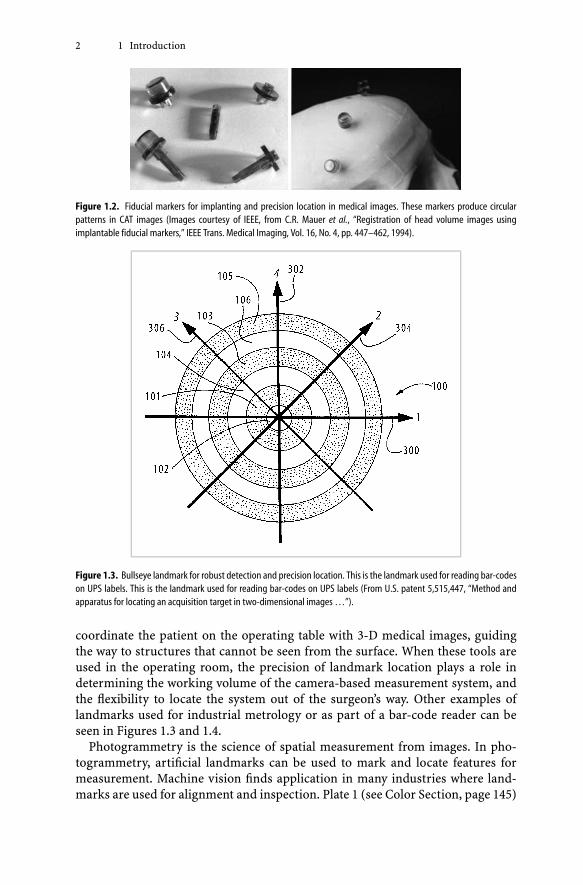
Figure 1.3. Bullseye landmark for robust detection and precision location. This is the landmark used for reading bar-codeson UPS labels. This is the landmark used for reading bar-codes on UPS labels (From U.S. patent 5,515,447, “Method andapparatus for locating an acquisition target in two-dimensional images …”).
coordinate the patient on the operating table with 3-D medical images, guidingthe way to structures that cannot be seen from the surface. When these tools areused in the operating room, the precision of landmark location plays a role indetermining the working volume of the camera-based measurement system, andthe flexibility to locate the system out of the surgeon’s way. Other examples oflandmarks used for industrial metrology or as part of a bar-code reader can beseen in Figures 1.3 and 1.4.
Photogrammetry is the science of spatial measurement from images. In pho-togrammetry, artificial landmarks can be used to mark and locate features formeasurement. Machine vision finds application in many industries where land-marks are used for alignment and inspection. Plate 1 (see Color Section, page 145)

1 Introduction 3
Figure 1.4. Artificial landmarks for metrology (Images courtesy of G. Ganci, H. Handley, “Automation in videogrammetry,”Melbourne, FL: Geodetic Services Inc.)
shows artificial landmarks used for alignment or measurement steps in the printingand electronic industries.
The digital images considered in this work are broken into pixels, or pictureelements, which are the individual samples of the scene, as seen in Figure 1.5. Thechallenge of landmark location is to accurately estimate the projection in the imageof the center of the landmark. Figure 1.5 illustrates the case where the landmarkoccupies relatively few pixels, which is the most challenging case and a commonone in image measurement applications, because space is limited in both the imageand in the scene in which the landmark lies. The measured intensity levels, onequantized value per pixel, are the data available for landmark location estimation.
Automated assembly and inspection, vision-guided robotic manipulation, pho-togrammetry, image metrology and camera calibration all benefit from preciselandmark location, and so it is useful to know how accurately artificial land-marks can be located digital images. It is well known that subpixel accuracy canbe achieved; but to answer the question of whether a landmark can be locatedwith an accuracy of ±0.1, 0.01 or 0.001 pixels requires detailed consideration. Thiswork aims to answer the question of landmark location precision by establishingthe theoretical minimum uncertainty that any location estimator can achieve, bydeveloping tools for evaluating the uncertainty of practical estimators, and by pre-senting an experiment for directly measuring landmark location precision. Thefruits of these labors can be used to determine the accuracy of a specified system,or to engineer a system to meet an accuracy goal. As O’Gorman et al. point out,
Figure 1.5a,b. Circular landmark; a ideal image of the landmark, b digital image of the landmark. Each picture element ofthe digital image corresponds to a measured intensity level (or three measured intensities for color images).

4 1 Introduction
“… the benefits of methods that achieve subpixel precision can be seen from twoperspectives: either as a means to obtain a higher precision, or as a means to obtainthe same precision at less computational cost.” (O’Gorman et al. 1990).
Since the present work is quite narrowly focused, it is worth mentioning whatthe present work is not. It is not a study of the entire range of questions that arisewhen measuring from images. In particular, the question of how a landmark isdetected is neglected. For automated image processing this is an important andchallenging question, but for the present purposes it is assumed that the presenceof the landmark in the image is known, along with its approximate location. Fur-thermore, the sources of uncertainty considered are restricted to those that arisewith the imaging and estimation processes, which is to say that any uncertaintyin the shape of the landmark itself is neglected. This is effectively a restriction towell-made artificial landmarks. Indeed, in the numerical and experimental stud-ies of the present report only planar-circular landmarks are considered, althoughthe methods extend to other shapes. Here, the only concern is with the locationof the landmark in the image, and so, although the numerical tool incorporatesa lens distortion model, displacement of the landmark in the image due to lensdistortion does not affect the conclusions. Finally, only digital images are con-sidered; that is, images that are quantized both in space (pixels) and intensity.This is more a challenge than a simplification, since the main theoretical chal-lenge of this work is to deal with quantization processes when determining theuncertainty. Narrowly focused as it is, the present work does have these chiefaims:
1. To introduce a measure for landmark location uncertainty that overcomes thenonstationary statistics of the problem.
2. To develop an extended model for the physics of image formation, capturingaspects of the physical process that contribute to the determination of theuncertainty.
3. To establish the Cramér–Rao lower bound (CRLB) for the uncertainty of land-mark location, given a description of the landmark and imaging configuration.The CRLB establishes a minimum level of uncertainty for any unbiased esti-mator, independent of the algorithm used.
4. To build a set of tools for analyzing the uncertainty of practical landmarkand imaging configurations and location estimation algorithms, taking intoaccount the spatial and intensity quantization in the image and the nonsta-tionary nature of the statistics in particular.
5. To demonstrate new, model-based landmark location estimators that performnear the Cramér–Rao theoretical limit.
6. To validate these tools by developing and executing an experiment that candirectly measure the uncertainty in landmark location estimates. The principalchallenge to experimental validation is to provide a means to separately andaccurately establish the true location of a landmark in the image.
These six goals form the basis for the remainder of the work.
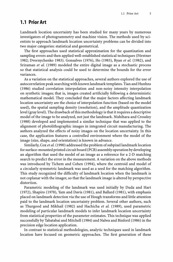
1.1 Prior Art 5
1.1 Prior Art
Landmark location uncertainty has been studied for many years by numerousinvestigators of photogrammetry and machine vision. The methods used by sci-entists to approach landmark location uncertainty problems can be divided intotwo major categories: statistical and geometrical.
The first approaches used statistical approximation for the quantization andsampling errors and then applied well-established statistical techniques (Förstner1982; Dvornychenko 1983). Gonsalves (1976), Ho (1983), Ryan et al. (1982), andSriraman et al. (1989) modeled the entire digital image as a stochastic processso that statistical analysis could be used to determine the bounds for the errorvariances.
As a variation on the statistical approaches, several authors explored the use ofautocorrelation peak searching with known landmark templates. Tian and Hunhns(1986) studied correlation interpolation and non-noisy intensity interpolationon synthetic images; that is, images created artificially following a deterministicmathematical model. They concluded that the major factors affecting landmarklocation uncertainty are the choice of interpolation function (based on the modelused), the spatial sampling density (resolution), and the amplitude quantizationlevel (gray level). The drawback of this methodology is that it requires a descriptivemodel of the image to be analyzed, not just the landmark. Nishihara and Crossley(1988) developed and implemented a similar technique that was applied to thealignment of photolithographic images in integrated circuit manufacturing. Theauthors analyzed the effects of noisy images on the location uncertainty. In thiscase, the application features a controlled environment where the model of theimage (size, shape, and orientation) is known in advance.
Similarly, Cox et al. (1990) addressed the problem of subpixel landmark locationfor surface-mounted printed circuit board (PCB) assembly operation by developingan algorithm that used the model of an image as a reference for a 2-D matchingsearch to predict the error in the measurement. A variation on the above methodswas introduced by Tichem and Cohen (1994), where the centroid and model ofa circularly symmetric landmark was used as a seed for the matching algorithm.This study recognized the difficulty of landmark location when the landmark isnot coplanar with the imager, so that the landmark image is altered by perspectivedistortion.
Parametric modeling of the landmark was used initially by Duda and Hart(1972), Shapiro (1978), Yam and Davis (1981), and Ballard (1981), with emphasisplaced on landmark detection via the use of Hough transforms and little attentionpaid to the landmark location uncertainty problem. Several other authors, suchas Thurgood and Mikhail (1982) and Hachicha et al. (1989), used parametricmodeling of particular landmark models to infer landmark location uncertaintyfrom statistical properties of the parameter estimates. This technique was appliedsuccessfully by Tabatabai and Mitchell (1984) and Nalwa and Binford (1986) in theprecision edge location application.
In contrast to statistical methodologies, analytic techniques used in landmarklocation have focused on geometric approaches. The first generation of these

6 1 Introduction
Tabl
e1.
1.M
appi
ngof
rele
vant
publ
icat
ions
vs.k
eyel
emen
tsfo
rlan
dmar
klo
catio
nun
cert
aint
y

1.1 Prior Art 7
Tabl
e1.
1.(c
ontin
ued)

8 1 Introduction
Tabl
e1.
2.Su
mm
ary
ofre
sear
chev
olut
ion
forl
andm
ark
loca
tion
unce
rtai
nty

1.1 Prior Art 9
Tabl
e1.
2.(c
ontin
ued)

10 1 Introduction
techniques was based on binary digital images, disregarding gray levels. Kulpa(1979) provided an in-depth geometrical analysis of the properties of digitalcircles, but Hill (1980) was the first to provide a rigorous geometrical analysisof landmark location uncertainty for a variety of geometrical shapes based onsynthetic binary images. Subsequently, several investigators reported a varietyof algorithms for improving error performance for particular landmark shapes.Vossepoel and Smeulders (1982), Dorst and Smeulders (1986), and Berenstein etal. (1987) focused on calculating uncertainty in the location of straight spatiallyquantized lines. Nakamura and Aizawa (1984) investigated the expansion of thiswork to circular landmarks, while Amir (1990) and Efrat and Gotsman (1994)presented new methodologies for locating the center of a circular landmark andDoros (1986) worked on the geometrical properties of the image of digital arcs.Bose and Amir (1990) investigated how landmark location uncertainty is affectedby the shapes and sizes of the binary images of various landmarks, concludingthat circular shapes provide superior performance. Similarly, O’Gorman (1990),O’Gorman et al. (1996), and Bruckstein et al. (1998) investigated novel shapes(bullseye and others), which improved the uncertainty performance for binaryimages.
The second generation of analytic techniques focused on the exploitation ofthe gray-level information, taking advantage of more bits in the intensity quan-tization. The use of grayscale intensity quantization improves landmark locationuncertainty (Rohr 2001). One of the first algorithms to make use of grayscaleinformation was developed by Hyde and Davis (1983), which gave results sim-ilar to the ones obtained for binary images. Klassman (1975) proved that forany finite spatial sampling density (density of pixels per area), the position un-certainty of a line was greater than zero, even when using unquantized images;that is, images whose amplitude is a continuous function. Kiryati and Bruck-stein (1991) showed how location uncertainty performance on binary image couldbe improved by the use of gray-level digitizers. Chiorboli and Vecchi (1993)showed empirically that the uncertainty performance of the results from Boseand Amir could be improved by an order of magnitude by using gray-level infor-mation.
Of particular importance is the locale framework proposed by Havelock (1989,1991) and expanded by Zhou et al. (1998). This methodology is based on theconcept of regions of indistinguishable object position, called locales, caused byspatial and intensity quantization. In the absence of noise, an observed digi-tal (quantized) image of a landmark corresponds to a region in which the truelandmark may lie. In general, this is a many-to-one mapping; that is, manydifferent landmark locations generate the same digital image. Havelock’s workmarked a great leap forward in analytic determination of landmark location un-certainty.
Table 1.1 shows how selected research publications address aspects of imageformation that are important for landmark location uncertainty. A summary ofthe research evolution for landmark location uncertainty is shown in Table 1.2. Asthe table reflects, research has been directed toward understanding and reducinglandmark location uncertainty for over three decades.
1.2 Modeling Image Formation 11
1.2 Modeling Image Formation
In this section, the approach of this work to modeling image formation is described.The goal is to capture the physical processes of image formation (such as propertiesof the camera and imager) that are important when determining the ultimate limitsto landmark location uncertainty.
While many previous studies have focused on binary images, several investiga-tors have recognized the need to develop methods for subpixel landmark locationthat make more efficient use of the information present in the image. Havelock(1989), a pioneer in the investigation of landmark location uncertainty, points outthat “it is not trivial to answer these questions [of landmark location uncertaintywith grayscale information] in a complete and meaningful way. This is a new areaof investigation, with only few results available at present.” Similarly, the work ofBruckstein et al. (1998) recommends further research into the exploitation of thegray-level information to improve precision in landmark location.
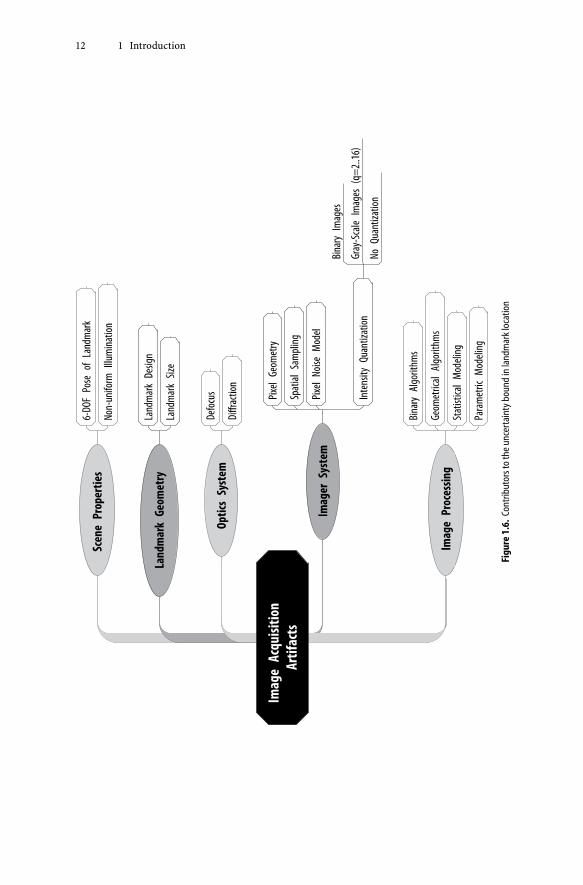
Grayscale information is only one of the characteristics that influence land-mark location uncertainty. An extensive model of image formation comprisescontributions from several scientific fields: physics (optics), electronics (imager),and computer science (image processing and estimation algorithms). The researchframework presented here introduces a methodology to determine the minimal un-certainty bound in landmark location based on the Cramér–Rao lower bound. TheCRLB methodology considers an extensive model of image formation, includingsix degree-of-freedom (DOF) landmark to camera geometry, diffraction, defocus,lens distortion, grayscale, pixel geometry, and pixel sensitive area. A list is shownin Figure 1.6 of the aspects of the image formation process that are consideredin this work. The Cramér–Rao lower bound methodology provides a theoreticalstatistical minimum limit on the landmark location uncertainty. Knowledge ofthis bound provides the means to evaluate the actual performance of both existingand future landmark location estimators. With this model, a general frameworkis established to measure the uncertainty performance of existing landmark lo-cation estimators, e.g., binary, geometrical, autocorrelation, statistical modeling,and others.
An important challenge to addressing uncertainty in landmark location is thatthe statistics of landmark location are not stationary. That is to say, the theoreticalCRLB as well as the covariance and bias of practical estimators all depend onwhere the landmark falls on the imager. This characteristic is associated with thelocales and raises the question of how to express uncertainty, since the covariancematrix itself varies significantly with small shifts of the true landmark location.A method is needed which averages over the range landmark locations and yetconveys information of practical engineering significance. At the same time, themethod chosen to express uncertainty should be applicable to all three of themeasures sought: the Cramér–Rao lower bound, analysis of practical estimators,and experimental measurement.
The confidence interval has been chosen to express landmark location uncer-tainty. The confidence interval is expressed as the radius of a circle in the digitalimage that will hold 95% (or in some cases 99%) of estimated landmark locations.
12 1 Introduction
Figu
re1.
6.Co
ntrib
utor
sto
the
unce
rtai
nty
boun
din
land
mar
klo
catio
n
1.2 Modeling Image Formation 13
In Chapter 3, methods for evaluating the confidence interval for the CRLB andanalytic cases are described in detail. For the experimental data, the confidenceintervals are obtained simply by determining the smallest circle that will enclose95% of the data. While coordinates of millimeters or microns on the imager arepreferred over pixel coordinates for image metrology, we have chosen to expressthe confidence interval in millipixels because landmark location estimators op-erate on pixel data. It is recognized that a circle measured in pixels translates, ingeneral, to an ellipse in image coordinates.
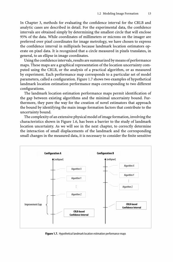
Using the confidence intervals, results are summarized by means of performancemaps. These maps are a graphical representation of the location uncertainty com-puted using the CRLB, or the analysis of a practical algorithm, or as measuredby experiment. Each performance map corresponds to a particular set of modelparameters, called a configuration. Figure 1.7 shows two examples of hypotheticallandmark location estimation performance maps corresponding to two differentconfigurations.
The landmark location estimation performance maps permit identification ofthe gap between existing algorithms and the minimal uncertainty bound. Fur-thermore, they pave the way for the creation of novel estimators that approachthe bound by identifying the main image formation factors that contribute to theuncertainty bound.
The complexity of an extensive physical model of image formation, involving thecharacteristics shown in Figure 1.6, has been a barrier to the study of landmarklocation uncertainty. As we will see in the next chapter, to correctly determinethe interaction of small displacements of the landmark and the correspondingsmall changes in the measured data, it is necessary to consider the finite sensitive
Figure 1.7. Hypothetical landmark location estimation performance maps
14 1 Introduction
area of each pixel and also the smoothing of the image introduced by diffraction.Since the sensitivity of the image data to the landmark location is essential to thisstudy, neither characteristic can be neglected. However, modeling finite sensitivearea requires integration of the incident light intensity (called the illuminancefunction) over the two-dimensional sensitive area of each pixel, and this integralcannot be performed in closed form. Indeed, because of the 2-D convolutionrequired to model diffraction-induced smoothing of the illuminance function, theilluminance function itself cannot be expressed in closed form for any case otherthan a straight edge.
The strategy used here to address these challenges employs a mix of analysis,where feasible, and numerical work where required. The inclusion of diffraction inthe analysis of landmark location uncertainty is an important innovation, becausethe smoothing of the illuminance function by diffraction enables rigorous numeri-cal analysis. In particular, the partial derivatives of the probability distributions ofthe measured data with respect to the location of the landmark, which are neededto compute the CRLB and also the performance of practical estimators, are well de-fined, well behaved, and can be computed only because diffraction assures us thatthe illuminance function has no discontinuities. This motivates the incorporationof diffraction as part of the model of image formation.
This work also introduces two novel circular landmark location estimationalgorithms, which perform with confidence intervals at the tens of millipixels level.This level of uncertainty is several times lower than that of a more conventionalcentroid algorithm. These algorithms are demonstrated for circular landmarks, butthe model-based methodology can be extended to accommodate other landmarkdesigns.
The first new landmark location estimator is named the “ellipsoidal contour”algorithm. It exploits the gray-level information present in the image by identify-ing points on a grayscale contour around the landmark, and then estimating theparameters of an ellipse fit to the contour. The second estimator, named “Butter-worth tepuy”, also exploits gray-level information by creating a parametric modelof the intensity surface of the landmark, while considering the smoothing causedby diffraction.
To experimentally measure the uncertainty of a landmark location algorithm,it is necessary to have an independent measurement of the true location in theimage of the landmark. This challenge is met by designing a second artwork thatsurrounds and is much larger than the primary landmark. By averaging overhundreds of pixels along the boundaries of this artwork, a reference location isdetermined for evaluating location estimators applied to the much smaller primarylandmark. The design incorporates an internal measure of location accuracy, toverify that the larger secondary landmark has been located more accurately thanthe Cramér–Rao lower bound for the location uncertainty of the primary landmark.
In summary, the present work establishes—for the first time—the minimumuncertainty in landmark location attainable, considering an extensive physicalmodel of image formation. With this bound, landmark location performancemaps are created to show the gap between the uncertainty achieved by practicallandmark location methodologies and the uncertainty bound. Moreover, novel
1.3 Mathematical Symbols and Nomenclature 15
landmark location estimation algorithms are introduced that achieve uncertaintylevels that closely approach the Cramér–Rao lower bound. Finally, experimentalresults are presented to validate the theoretical findings.
1.3 Mathematical Symbols and Nomenclature
The discussion of landmark location accuracy will involve details of geometryexpressed in several coordinate frames. A notation that captures the type of repre-sentation, the point referred to and the coordinate frame of reference will providea compact way to discuss landmark geometry unambiguously. The notation usedby J.J. Craig (1986) and others is described here and used throughout this work.Notation related to signals and estimation is also described. In addition to thissection, a list of symbols is provided in Appendix A.
1.3.1 Coordinate Systems
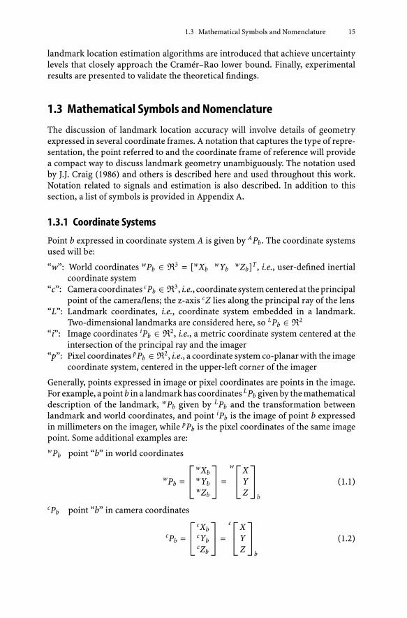
Point b expressed in coordinate system A is given by APb. The coordinate systemsused will be:
“w”: World coordinates wPb ∈ R3 = [wXbwYb
wZb]T , i.e., user-defined inertialcoordinate system
“c”: Camera coordinates cPb ∈ R3, i.e., coordinate system centered at the principalpoint of the camera/lens; the z-axis cZ lies along the principal ray of the lens
“L”: Landmark coordinates, i.e., coordinate system embedded in a landmark.Two-dimensional landmarks are considered here, so LPb ∈ R2
“i”: Image coordinates iPb ∈ R2, i.e., a metric coordinate system centered at theintersection of the principal ray and the imager
“p”: Pixel coordinates pPb ∈ R2, i.e., a coordinate system co-planar with the imagecoordinate system, centered in the upper-left corner of the imager
Generally, points expressed in image or pixel coordinates are points in the image.For example, a point b in a landmark has coordinates LPb given by the mathematicaldescription of the landmark, wPb given by LPb and the transformation betweenlandmark and world coordinates, and point iPb is the image of point b expressedin millimeters on the imager, while pPb is the pixel coordinates of the same imagepoint. Some additional examples are:wPb point “b” in world coordinates
wPb =
⎡⎣
wXbwYbwZb
⎤⎦ =
w⎡⎣
XYZ
⎤⎦
b
(1.1)
cPb point “b” in camera coordinates
cPb =
⎡⎣
cXbcYbcZb
⎤⎦ =
c⎡⎣
XYZ
⎤⎦
b
(1.2)

16 1 Introduction
LPa point “a” in landmark coordinates
LPa =[
LXaLYa
]=
L[XY
]
a(1.3)
1.3.2 Origin of the Coordinate System
The origin is a special point in a coordinate frame. The origin of coordinate frame Aexpressed in coordinate frame D is denoted as DPo
A. The upper-left subscript may
be omitted when a general reference to the origin of the coordinates system ismade. Several examples are:
Center of a landmark in camera coordinates:
cPoL
=
⎡⎢⎢⎣
cXoL
cYoL
cZoL
⎤⎥⎥⎦ =
c⎡⎣
XYZ
⎤⎦
oL
(1.4)
Origin of the image coordinates:
Poi
(1.5)
The image location of the center of the landmark, expressed in pixel coordi-nates:
pPoL
(1.6)
aP b Symbol aP b designates a six-dimensional pose of a coordinate frame b ex-pressed in coordinate frame a. An example used in the development is cPo
L,
which is the pose of the landmark expressed in camera coordinates:
cPoL
= [cx cy cz ω κ ϕ]T , (1.7)
where [cx cy cz]T is the 3-DOF position of the landmark in the cameraframe, and where ω = pitch, κ = roll and ϕ = yaw angles of the orientationof the landmark in the camera frame. For this work, the rotation order forthe rotation from target to camera coordinates is R = Rκ Rϕ Rω, where each Ris a 3 × 3 rotation matrix.
1.3.3 Image Formation
The following subsection describes the nomenclature and mathematical symbolsthat will be used at each stage of the image formation model. The image formationmodel is described in detail in Chapter 2.

1.3 Mathematical Symbols and Nomenclature 17
Landmark luminosity function:
Function that provides the definition of the landmark geometry on the landmarkplane,
f L(Lx, Ly) , (1.8)
expressed in lumens or per unit.
Optical flux function:
Function representing the spatial distribution of illumination of the imager con-sidering geometric optics:
H(ix, iy) = Φ(
Gf
(cPo
L, f L(Lx, Ly)
)), (1.9)
expressed in lux or per unit.
Illuminance function:
Function representing the optical flux on the imager after the addition of thediffraction phenomena:
E(ix, iy) = Ξ(H(ix, iy)
), (1.10)
expressed in lux or per unit.
Discrete analog intensity function:
Function describing the illuminance function after spatial quantization:
J(i, j) = Qs(E(ix, iy)
)(1.11)
expressed in charge or per unit.
Digital image:
Function describing the discrete analog intensity function after amplitude quan-tization:
I = Qi(J(i, j)) , (1.12)
expressed in units of counts on a range determined by the A/D converter, or perunit with 1 = full scale.

18 1 Introduction
1.3.4 Estimation Basics
Estimation is the statistical discipline that involves estimating the values of modelparameters based on measured data. Much of the present work employs the toolsof a multivariable statistical framework with a focus on estimation theory. Thefollowing mathematical notation is used throughout.
The true value of a given parameter vector θ is marked with a star:
θ∗ . (1.13)
The estimated value of a given parameter θ is marked with a hat:
θ . (1.14)
The misadjustment in the estimate of a give parameter θ is marked witha tilde: θ; that is,
θ = θ∗ + θ . (1.15)
The measurement of a data vector Y is written as: Y. For each measure-ment Y, there is an underlying but generally unknown true value, Y∗, andmeasurement error or noise, Y, with a relationship:
Y = Y∗ + Y . (1.16)
Examples:
• Estimated center of landmark in image coordinates:
iPoL
. (1.17)
• Estimated location of a point b in pixel coordinates:
pPb = pP∗b + pPb , (1.18)
where pPb represents estimator error.
• Measured digital image in the presence of noise:
I = QI(J) = QI(J∗ + J) , (1.19)
where J is noise in the discrete analog intensity function and QI(·) is the intensity
quantization function.
• Noise in the measurement of the digital image:
I = I∗ − I . (1.20)

1.4 Content Organization 19
1.3.5 Estimators
The landmark location estimators are algorithms that take image data and pro-duce a landmark location estimate, written pP0 = T
(I). Four landmark location
estimators are considered; these are denoted by TA( ), TB( ), TD( ), and TE( ), where:
TA( ) is the binary centroid estimator;TB( ) is the grayscale centroid estimator;TD( ) is the ellipsoidal contour estimator, and;TE( ) is the Butterworth tepuy estimator.
Some nomenclature examples for estimators follow:
• Binary centroid estimator on the discrete analog intensity function J:
pPoL
= TA(J) . (1.21)
• Butterworth tepuy estimator applied to the digital image function I:
pPoL
= TE(I) . (1.22)
• Estimate of the center of the landmark in pixel coordinates using the ellipsoidalestimator:
pPoL
= TD(I) . (1.23)
1.4 Content Organization
The subsequent chapters are organized as follows. Chapter 2 addresses modelingissues, with the extensive physical model of digital image formation developed inSection 2.1. Locales and the use of confidence intervals are discussed in Section 2.2.The necessary analytic tools are developed in Chapter 3, with tools for forming theconfidence interval based on the Cramér–Rao lower bound derived in Section 3.1and tools for analyzing the performance of practical estimators derived in Sec-tion 3.2. The details of two new, model-based landmark location estimators arepresented in Chapter 4. Calculation of both the CRLB and practical estimator per-formance requires an innovation in 2-D numerical integration, which is the topicof Chapter 5. The computational tool that generates the landmark location uncer-tainty performance maps is presented in Chapter 6. In Chapter 7 an experimentalmethod is presented which can directly and accurately measure the uncertainty inlocating a primary landmark, based on the estimated location of a much larger andmore accurate secondary landmark. This is followed in Chapter 8 by the presen-tation of experimentally measured landmark location uncertainty, which is usedto validate the analytic tools of Chapter 3, as well as the results from numericalinvestigations employing the analytic tools to study the impact on location accu-racy of a range of configuration variables. Finally, the conclusions of this work arepresented in Chapter 9.

20 1 Introduction
A downloadable MATLAB® package to assist the reader with applying theoret-ically-derived results to practical engineering configurations is available fromhttp://www.springer.com/978-1-84628-912-5.

2 Physics of Digital Image Formation
We begin our discussion of modeling by addressing why it is essential to considertwo phenomena that play a role in image formation, influence the precision oflandmark location, and have often been neglected in the past. These are thefinite sensitive area of each pixel and the smoothing of the illuminance functionintroduced by diffraction. The detection of landmark location is an estimationproblem, and the accuracy of any estimator is governed by the sensitivity of thedata to changes in the quantity to be estimated. For landmark location, this is(∂J/∂ pP∗
o
), where J ∈ RNp×1 is the discrete analog intensity values of Np pixels
used to estimate the landmark location, and pP∗o ∈ R2 is the true location of the
landmark. The intensity values are organized as an Np × 1 column vector so thatthe derivative
(∂J/∂ pP∗
o
)is a 2-D array. For this discussion, the analog intensity
values, J, are used rather than the digital image values, I, to avoid the complicationof intensity quantization. Consideration of intensity quantization is deferred toSection 3.2.1.
A hypothetical ideal image of a landmark is illustrated in Figure 2.1, which showsa 3 × 3 pixel grid with a two-pixel-diameter circular landmark. The white pointin each pixel indicates a simplified model of image formation in which each pixelis sampled at its center to determine the measurements of the digital image. Forexample, referring to the indices shown in parentheses in Figure 2.1, the digitalimage is given as:
J = [0.0 0.0 0.0 0.0 1.0 1.0 0.0 1.0 1.0]T , (2.1)
where a value of J(i) = 1.0 corresponds to a point inside the landmark image,and J(i) = 0.0 corresponds to a point in the background. With this model, whichcombines the point-wise sensitive area of the pixel with a discontinuous boundaryfor the landmark image, 0.0 and 1.0 are the only possible values of pixel intensity.This simplified model has been used in 36 of the 38 articles listed in Table 1.1.
An example showing the sensitivity of the data to changes in landmark locationis illustrated in Figures 2.2 and 2.4. These figures schematically show the circularlandmark and 3 × 3 grid of pixels of Figure 2.1. Like Figure 2.1, Figure 2.2 is drawnwith pixels modeled as having a sensitive area that is 0% of the pixel area, andno smoothing at the edge of the landmark. In the left portion of Figure 2.2, thelandmark is shown at location pP∗
1 = [2.45 2.40]T , and in the right portion it isat location pP∗
1 = [2.45 2.35]T . Ordering the data in a column vector according to

22 2 Physics of Digital Image Formation
Figure 2.1. Illustration of the optical flux function corresponding to a circular landmark, shown on a digital imager. Thesquares indicate pixels, which are indexed by the numerals in parentheses. An example optical flux function, H(ix, iy), isshown, see Equation 1.9 above. Because the landmark has a sharp edge, the optical flux is discontinuous at the boundaryof the landmark. The white points in the centers of the pixels indicate 0% sensitive area.
indices shown in parentheses gives
J1 =
⎡⎢⎢⎢⎢⎢⎢⎢⎢⎢⎢⎢⎢⎣
0.00.00.00.01.01.00.01.01.0
⎤⎥⎥⎥⎥⎥⎥⎥⎥⎥⎥⎥⎥⎦
J2 =
⎡⎢⎢⎢⎢⎢⎢⎢⎢⎢⎢⎢⎢⎣
0.00.00.00.01.01.00.01.01.0
⎤⎥⎥⎥⎥⎥⎥⎥⎥⎥⎥⎥⎥⎦
ΔJ/Δ pY∗o =
⎡⎢⎢⎢⎢⎢⎢⎢⎢⎢⎢⎢⎢⎣
0.00.00.00.00.00.00.00.00.0
⎤⎥⎥⎥⎥⎥⎥⎥⎥⎥⎥⎥⎥⎦
, (2.2)
where ΔJ/Δ pY∗o is the change in image data arising with the change in landmark
location. In this example, even though the landmark has moved between the leftand right portions of Figure 2.2, the data are not modified. When finite sensitive
Figure 2.2. A circular landmark on a 3 × 3 pixel grid. The pixel data is organized into a column vector according to theindices shown in parentheses. The interior of the landmark is shown with cross-hatching. The center of the landmark isshown with a cross and marked pP∗
1 . The landmark covers the sensitive areas of pixels 5, 6, 8 and 9.

2 Physics of Digital Image Formation 23
Figure 2.3. Illustration of a landmark image with smoothing considered. An example illuminance function, E(ix, iy), isshown (see Equation 1.10 above). The smoothing effect of diffraction is approximated by convolving the intensity profileof Figure 2.1 with a Gaussian kernel. The illuminance function is continuous throughout the image, and in particular, at theboundary of the landmark. Pixel sensitive area is not shown.
area and smoothing are not considered, the model predicts an analog intensityfunction that is a piece-wise constant, discontinuous function of the landmarklocation; and the derivative of the data with respect to the landmark location iseither zero or infinity, either of which pose difficulties when examining estimatoruncertainty.
Figure 2.3 illustrates a simulated image of the same landmark seen in Figure 2.1,except that diffraction is incorporated into the model. To generate the illustrationof Figure 2.3, diffraction is approximated by convolution with a 2-D Gaussiankernel, as described in Section 2.1. Because of the smoothing effect of diffraction,the intensity of the image of the landmark is not discontinuous.
In Figure 2.4, a small displacement of the landmark is once again considered.Figure 2.4 is like Figure 2.2, except that the pixel sensitive area is modeled as 12%of the total pixel area, and the shaded ring illustrates a region of smooth transitionbetween the interior and exterior intensity of the landmark. In the transitionregion shown by the shaded ring, the illuminance function takes intermediate
Figure 2.4. A circular landmark on a 3 × 3 pixel grid with finite sensitive area. This figure is analogous to the previousfigure, but with finite sensitive areas and transition region shown. Pixel (2,2) will measure an illuminance correspondingfully to the landmark, while three other pixels will record partial illumination by the landmark.

24 2 Physics of Digital Image Formation
values between E(ix, iy) = 1.0 and E(ix, iy) = 0.0. On the right-hand side, as inFigure 2.2, the landmark is shifted by 0.05 pixels. Example data for Figure 2.4,along with the first difference of the data with respect to the pY position of thelandmark, are given as
J3 =
⎡⎢⎢⎢⎢⎢⎢⎢⎢⎢⎢⎢⎢⎣
0.00.00.00.01.000.900.000.950.70
⎤⎥⎥⎥⎥⎥⎥⎥⎥⎥⎥⎥⎥⎦
J2 =
⎡⎢⎢⎢⎢⎢⎢⎢⎢⎢⎢⎢⎢⎣
0.00.00.00.01.000.600.001.00.30
⎤⎥⎥⎥⎥⎥⎥⎥⎥⎥⎥⎥⎥⎦
ΔJ/Δ pY∗o =
⎡⎢⎢⎢⎢⎢⎢⎢⎢⎢⎢⎢⎢⎣
0.00.00.00.00.000.600.00
−1.000.80
⎤⎥⎥⎥⎥⎥⎥⎥⎥⎥⎥⎥⎥⎦
, (2.3)
The nonzero values of the first difference show that there is a signal with whichto detect the change of location of the landmark. The first difference above relatesto the derivatives that are developed theoretically in Section 3.1.1 and computedwith the tools described in Chapter 6.
There are several issues that are illustrated by the examples of Figure 2.1 throughFigure 2.4 that should be noted:
• With the simplified model of Figure 2.2, the data do not contain any indication ofa small shift in the landmark location. These figures show an oversimplification,because actual imagers have finite sensitive area—in most cases greater than 12%fill factor—and actual illuminance distributions have finite transition regions.
• Because diffraction gives a smooth transition from background to landmarkilluminance levels, the derivative of the data with respect to the landmark lo-cation is mathematically well posed. Smoothing makes the calculation of theCramér–Rao lower bound possible.
• The pixel boundaries are artificial. It is the boundaries of the sensitive areas thathave physical significance and determine the connection between landmarkconfiguration and measured data. For convenience, the pixel boundaries are setso that the centroid of the pixels coincide with the centroid of the sensitive areas.
• The derivative of the image data with respect to displacements of the landmarkdepends on the location of the landmark. This gives rise to the nonstationarystatistics of landmark location estimation. These nonstationary statistics aretreated in Sections 3.1.2 for the Cramér–Rao lower bound, and 3.2.2 for theanalysis of practical estimators.
With these considerations, the formation of the digital image of a landmark canbe modeled as a set of transformations that start with the geometrical definitionof the landmark and lead to a spatially quantized and intensity-quantized imagearray I(i, j), or digital image. Image formation can be modeled in five stages:

2 Physics of Digital Image Formation 25
1. First, the 6-DOF pose of the landmark in camera coordinates is passed
through a landmark description transformation Gf
(cPo
L, f L
(Lx, Ly
)), creat-
ing the landmark luminosity function f L(cx, cy, cz).
2. The landmark luminosity function is then transformed by the geometric opticstransfer function Φ, creating the optical flux function H(x, y). A pinhole cameramodel is used (Hecht and Zajac 1979). A sample optical flux function is shownin Figure 2.1.
3. The optical flux function is then low-pass-filtered by the transfer function Ξ,creating the illuminance function E(x, y). The low-pass filtering models thediffraction of the light passing through the camera aperture, as predicted by
Figure 2.5. Geometric Optics and Coordinate System Definition

26 2 Physics of Digital Image Formation
Fourier optics. An example illuminance function, corresponding to the opticalflux function of Figure 2.1, is illustrated in Figure 2.3.
4. The Illuminance function is processed by the image transducer, or imager,which performs a spatial sampling transformation Qs, yielding the discreteanalog intensity function J(i, j).
5. Finally, the amplitude of the discrete analog intensity function is quantized bythe transformation Qi, creating the digital image, I(i, j).
Figure 2.6. Generation of a digital image

2 Physics of Digital Image Formation 27
The coordinate frames of the geometric optical model are illustrated in Fig-ure 2.5. Figure 2.6 shows the model chain of transformations. The mathematicalnomenclature used in Equation 2.4 is presented in Section 1.3 above, and is listedin Appendix A.
The model chain of transformations is shown in functional form in Equation 2.4.The last transformation presented in Equation 2.4 corresponds to the estimationof the location of the landmark.
cPoL
=
⎡⎢⎢⎢⎢⎢⎢⎣
cxcyczωκϕ
⎤⎥⎥⎥⎥⎥⎥⎦
Gf→ f (Lx, Ly)Φ→ H(ix, iy)
Ξ→ E(ix, iy)Qs→ J(pi, pj) →
→ ⊕↑
J(pi, pj)
Qi→ I(pi, pj)T→ iPo
L. (2.4)
Notice that image noise J(x, y) is added at the stage just before the intensity quan-tization; physically this noise model is consistent with the properties of practical
Figure 2.7. Simplified model of digital image formation used in past studies

28 2 Physics of Digital Image Formation
imagers. Furthermore, in this model, as in practical image acquisition systems,it is assumed that the optical flux function is of finite support; that is, the re-gion Ω in which it is nonzero has finite extent; this is expressed mathematically inEquation 2.5.
H(x, y) = 0 {(x, y) /∈ Ω} . (2.5)
In the previous studies of landmark location uncertainty listed in Tables 1.1 and 1.2,it was common to assume a discontinuous transition in the illuminance functionat the edge of the image of the landmark, and to treat the spatial sampling processas impulsive; that is, to model the photosensitive area of the pixel as a point in thesampling plane. For comparison with Equation 2.4 and Figure 2.6, Equation 2.6and Figure 2.7 show the simplified model of digital image formation that has beenused in many previous studies.
F(Lx, Ly)Φ→ H(ix, iy)
Qs→ J(i, j)Qi→ I(i, j) . (2.6)
2.1 Image Formation and Landmark Location Uncertainty
Landmark location uncertainty is affected by a variety of artifacts in the imageacquisition process. As indicated in Figure 1.6, these artifacts can be classified intofive groups: scene properties, landmark geometry, optics system, imager system,and the selection of the image-processing algorithm. The following paragraphsprovide an overview of how these artifacts participate in the overall uncertainty inlandmark location.
2.1.1 Scene Properties
The two main scene properties that affect the landmark location process are thesix degree-of-freedom (6-DOF) pose of landmark and nonuniform illumination.When the landmark is tilted with respect to the optical axis of the camera, itwill give rise to perspective distortion in the image of the landmark. Nonuniformillumination can introduce bias into the location estimator.
The effects of perspective distortion can be visualized by means of a simpleexample. Figure 2.8 illustrates the influence of landmark tilt. In this figure, por-tions of the landmark that are closer to the camera appear larger than portionsfarther away from it, causing the overall shape of the landmark to be distorted.Consequently, the centroid of the image of the landmark no longer corresponds tothe image of the centroid of the landmark. Full perspective distortion is consideredhere through the use of analytic tools developed in this work. Landmark locationerrors arising with tilt are investigated in Section 8.6.
Nonuniform illumination causes intensity variations in the image that may causebias in the image-processing algorithm. Landmark location errors that arise withtilt are investigated in Section 8.8.

2.1 Image Formation and Landmark Location Uncertainty 29
Figure 2.8. Example of the effects of perspective distortion in landmark location
2.1.2 Landmark Geometry
The landmark shape directly impacts on the landmark location uncertainty (Boseand Amir 1990; Amir 1990; O’Gorman et al. 1990). Normally, the impact on loca-tion uncertainty depends on the type of image processing algorithm (Brucksteinet al. 1998). Typical landmark shapes used are shown in Figure 2.9. Usually, land-marks with circular symmetry are preferred due to their rotational invariance andanalytically simple formulation (Bose and Amir 1990).
Figure 2.9. Typical landmark shapes used in the literature

30 2 Physics of Digital Image Formation
Similarly, the size of the landmark with respect to the scene captured effects thelocation uncertainty. The landmark size determines the number of pixels carryinginformation that the image-processing algorithm can exploit.
2.1.3 Optics System
The optical system of the camera forms the flux function of the scene on theimager sensor. Optical phenomena such as diffraction and defocus influence theuncertainty of landmark location.
Diffraction
Diffraction is the phenomenon that occurs when light deviates from straight-line propagation in a way that cannot be interpreted as reflection or refraction.Diffraction arises when light waves are partially blocked by obstacles (Hecht andZajac 1979). Optical devices, such as cameras, collect a limited portion of theincident light wavefront from the scene; this inevitably introduces diffraction (Sears1979), which is perceived as smoothing of the image. The degree of smoothing isa function of the geometry of the camera aperture and its size relative to λ, thewavelength of light being captured. In the conceptual limit when λ → 0, thediffraction effect no longer exists and all of the ideal geometrical optics lawsapply.
A model of diffraction is incorporated into this study for two reasons: thesmoothing of the illuminance function by diffraction influences the performance oflandmark location estimators, and it also makes the required numerical integrationof the illuminance function possible. Without smoothing the illuminance function,the analytic results of this study would not be possible.
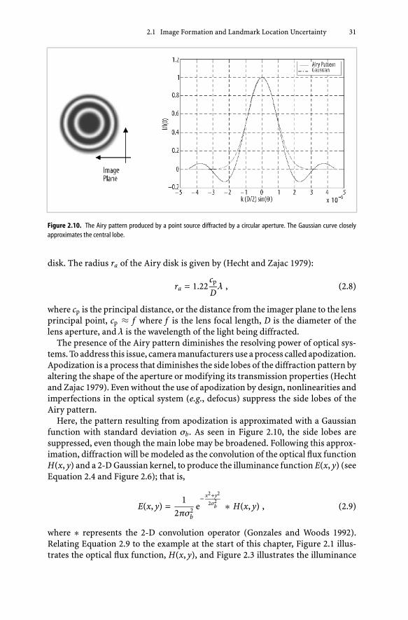
The diffraction pattern caused by a circular aperture is called the Airy pattern(Figure 2.10) and is described by:
I(θ) = I(0)
[2J1
(k D
2 sin θ)
k D2 sin θ
]2
, (2.7)
where I(0) is the maximum illuminance at the center of the pattern, D is thediameter of the circular aperture, k = 2π
λ is the propagation number, J1 in theequation above is the Bessel function of the first kind and order 1, and θ is theangle formed between the principal ray and a vector from the principal point
toward a point (x, y) in the image plane; that is, tan(θ) =√
ix2 + iy2
cp. Justification of
this equation comes from the Fraunhofer approximation to the Huygens–Fresnelprinciple and the use of circular apertures (Goodman 1968).
The first dark ring of the Airy pattern has a flux density of about 1.75% that ofthe central ring. About 84% of the light incident on the image is distributed in themain lobe of the Airy pattern. The central disk of this pattern is called the Airy
2.1 Image Formation and Landmark Location Uncertainty 31
Figure 2.10. The Airy pattern produced by a point source diffracted by a circular aperture. The Gaussian curve closelyapproximates the central lobe.
disk. The radius ra of the Airy disk is given by (Hecht and Zajac 1979):
ra = 1.22cp
Dλ , (2.8)
where cp is the principal distance, or the distance from the imager plane to the lensprincipal point, cp ≈ f where f is the lens focal length, D is the diameter of thelens aperture, and λ is the wavelength of the light being diffracted.
The presence of the Airy pattern diminishes the resolving power of optical sys-tems. To address this issue, camera manufacturers use a process called apodization.Apodization is a process that diminishes the side lobes of the diffraction pattern byaltering the shape of the aperture or modifying its transmission properties (Hechtand Zajac 1979). Even without the use of apodization by design, nonlinearities andimperfections in the optical system (e.g., defocus) suppress the side lobes of theAiry pattern.
Here, the pattern resulting from apodization is approximated with a Gaussianfunction with standard deviation σb. As seen in Figure 2.10, the side lobes aresuppressed, even though the main lobe may be broadened. Following this approx-imation, diffraction will be modeled as the convolution of the optical flux functionH(x, y) and a 2-D Gaussian kernel, to produce the illuminance function E(x, y) (seeEquation 2.4 and Figure 2.6); that is,
E(x, y) =1
2πσ2b
e− x2+y2
2σ2b ∗ H(x, y) , (2.9)
where ∗ represents the 2-D convolution operator (Gonzales and Woods 1992).Relating Equation 2.9 to the example at the start of this chapter, Figure 2.1 illus-trates the optical flux function, H(x, y), and Figure 2.3 illustrates the illuminance

32 2 Physics of Digital Image Formation
function, E(x, y). For the approximation of Figure 2.10, the 2-D Gaussian kernel isrelated to the Airy pattern by
σb =ra
2. (2.10)
The radius of the Airy disk can also be related to camera parameters. By definition,the focal number, F/#, is given as the relation between the lens focal length andthe diameter of the camera aperture; that is,
F/# =fD
. (2.11)
The wavelength range of visible light is:
λ = 780 … 390 nm . (2.12)
For λ = 780 nm, we get a useful value for the radius of the smoothing operator of:
ra = 1.22F/#λ ≈ F/# (in microns) . (2.13)
This implies that the radius of the Airy disk can be approximated by the F/# inmicrons. Using Equation 2.10 and Equation 2.13 we get:
σb =12
F/# (in microns) . (2.14)
For practical systems, the radius of the smoothed pattern given as the image ofa small point should be measured and related to the radius of a 2-D Gaussian dis-tribution. Furthermore, some image acquisition systems specify the parameter σb.
Defocus
Departures from the diffraction-limited optical model are called aberrations (IEEE2000). The most common optical aberration is caused by defocus. The lens lawdetermines the focus condition:
1f
=1cp
+1
czoL
, (2.15)
where f is the focal length of the lens, cp is the distance from the principal pointof the lens to the imager, sometimes called the adjusted focal length, and czo
Lis the
distance from the lens to the observation plane, as indicated in Figure 2.11.Defocus creates a blurring effect on the image, which can be modeled by a suit-
able change in the convolution operator of Equation 2.9. The convolution operatorto model defocus is the image of the suitably scaled aperture (commonly a uni-form disk). Using Fourier optics, it can be shown that defocus lowers the contrastof each spatial frequency component of image intensity (Goodman 1968). Defo-cus increases the smoothing provided by diffraction. When the dimension of thesmoothing operator σb is small relative to the pixel size, additional smoothing can

2.1 Image Formation and Landmark Location Uncertainty 33
Figure 2.11. Geometry of the lens law, Equation 2.15
enhance location accuracy. Thus, there may be cases in which it is advantageousto deliberately defocus a camera for precision landmark location.
The tools developed in Chapters 3 and 6 support detailed analysis of landmarklocation uncertainty with specific levels of smoothing. Since the convolution ofEquation 2.9 cannot be performed in closed form, it is implemented numericallyusing the specialized 2-D integration technique presented in Chapter 5 to generatethe illuminance function for a particular configuration. Because of the informationlost in the regions between pixel sensitive areas, as seen in Figure 2.4, smoothingof the digital image by signal processing is not equivalent to smoothing of theilluminance function by defocus.
Lens Distortion
Lens distortion is a type of lens aberration that alters the location of the image ofthe landmark (Atkinson 1996). There are two types of lens distortions: radial anddecentering.
Radial distortion is caused by the curvature of the lens and consists of a radialdisplacement of the image of the landmark closer to or farther from the principalpoint. Radial distortion is normally expressed in the form known as balanced ∂rb,as:
∂rb = K0r + K1r3 + K2r5 + K3r7 + · · · [microns] (2.16)
where the constants Ki represent the coefficients of radial distortion and r is theradial distance from the principal point:
r2 =(ix − ixo
)2+(iy − iyo
)2 (ixo, iyo)
= Principal Point. (2.17)
In many cases the terms K0 and K1 are sufficient. For wide-angle lenses, higherorder terms may also be significant.
34 2 Physics of Digital Image Formation
Decentering distortion is caused by any displacement or rotation of a lens ele-ment from perfect alignment. This type of aberration is caused by manufacturingdefects, and it causes geometric displacement in images. The effects of decenteringdistortion are approximated in a truncated polynomial form as:
ΔxS =
(1 −
cp
czoL
) [P1
(r2 + 2
(ix − ixo)2)
+ 2P2(ix − ixo
) (iy − iyo)]
ΔyS =
(1 −
cp
czoL
) [P2
(r2 + 2
(iy − iyo)2)
+ 2P1(ix − ixo
) (iy − iyo)]
, (2.18)
where ΔxS, ΔyS represents the decentering distortion at an image point ix, iy; ris the radial distance as described in Equation 2.17,
(ixo, iyo
)are the coordinates
of the principal point, and cp is the adjusted focal length for a lens focused ata distance czo
L.
The distortion model of Equation 2.17 and Equation 2.19 is implemented inthe computation tools described in Chapter 6. In addition, the lens used in theexperimental section shown in Chapter 7 was calibrated by determining the lensdistortion parameters using a commercial tool.
2.1.4 Imager System
Several artifacts of the imager system participate in the determination of landmarklocation uncertainty. An overview of these artifacts follows.
The first artifact considered is spatial sampling. The 2-D sampling theorem isdiscussed. Whereas the sampling theorem provides that the band-limited sampledsignal can be completely reconstructed, the spatial frequency of the illuminancefunction is rarely, if ever, limited to the spatial frequency bandwidth describedby the sampling theorem. The significant consequence of this is a skew errorintroduced by spatial sampling, which appears as a bias in the estimate landmarklocation. An example with impulsive spatial sampling (infinitesimal pixel sensitivearea) and a 1.8-pixel-diameter landmark illustrates the bias.
Next finite sensitive area is considered, along with a model for noise in thediscrete analog intensity function. Finally, intensity quantization is considered.With these pieces in place, locales—regions in which the landmark can lie whichgive the same digital image—are considered in detail.
Spatial Sampling and Locales
The Whittaker–Shannon sampling theorem states that to recover a band-limited,continuous signal of bandwidth W from its samples without distortion, it is nec-essary to select a sampling interval Δx so that 1/Δx ≥ 2W (Ziemmer et al. 1983),or
Δx ≤ 12W
, (2.19)

2.1 Image Formation and Landmark Location Uncertainty 35
where Δx is the width of a pixel on the imager (in millimeters), and W (in cy-cles/mm) is the spatial bandwidth of the illuminance function. The sampling the-orem can be expanded for two-dimensional signals. In this case, the 2-D samplingtheorem states that a continuous band-limited function E
(ix, iy
)can be recovered
completely from samples whose separation is bounded by
Δx ≤ 12Wx
, (2.20)
Δy ≤ 12Wy
, (2.21)
where Wx and Wy represent the bandwidths of the signal in the x and y coordinatesrespectively. The estimate coordinates (x, y) of the unsampled illuminance functioncan be calculated estimating the centroid of the landmark; that is,
x =
∫∫Ω
x E(x, y) dx dy∫∫Ω
E(x, y) dx dy=
yu∫yl
xu∫xl
xE(x, y) dx dy
yu∫yl
xu∫xl
E(x, y) dx dy
and
y =
∫∫Ω
y E(x, y) dx dy∫∫Ω
E(x, y) dx dy=
yu∫yl
xu∫xl
yE(x, y) dx dy
yu∫yl
xu∫xl
E(x, y) dx dy
. (2.22)
From the Whittaker–Shannon sampling theorem, the same centroid estimate couldbe obtained from the samples of the band-limited signal, since the original unsam-pled function could be reconstructed from its samples from −∞ to ∞. However,an image function, just like all physical signals, is necessarily of finite extent, whichin turn implies that it cannot be band-limited and its samples will only be able toapproximate the original function.
An estimate of the centroid based on the samples of the illuminance functioncan be defined in the following manner:
xd =
xu−xlΔx∑
i=0
yu−ylΔy∑
j=0
(xl + iΔx
)E(xl + iΔx, yl + jΔy)
xu−xlΔx∑
i=0
yu−ylΔy∑
j=0E(xl + iΔx, yl + jΔy)

36 2 Physics of Digital Image Formation
and
yd =
xu−xlΔx∑
i=0
yu−ylΔy∑
j=0
(yl + jΔy
)E(xl + iΔx, yl + jΔy)
xu−xlΔx∑
i=0
yu−ylΔy∑
j=0E(xl + iΔx, yl + jΔy)
. (2.23)
The estimate (xd, yd) represents the discrete centroid of the illuminance functionE(x, y). The difference of this estimate from the actual position is referred to as theskew error; this error is caused by the spatial sampling process.
It can be shown that in the limit as the sampling interval goes to zero, the discretecentroid estimate is an unbiased estimator of the unsampled illuminance functioncentroid; that is, Δx → 0 and Δy → 0 implies that (xd, yd) → (x, y). The prooffollows from the integral definition applied to Equation 2.23:
LimΔx→0
LimΔy→0
(xd)
= LimΔx→0
LimΔy→0
ΔxΔy
xu−xlΔx∑
i=0
yu−ylΔy∑
j=0
(xl + iΔx
)E(xl + iΔx, yl + jΔy)
ΔxΔy
xu−xlΔx∑
i=0
yu−ylΔy∑
j=0E(xl + iΔx, yl + jΔy)
=
LimΔx→0
LimΔy→0
xu−xlΔx∑
i=0
yu−ylΔy∑
j=0xiE(xi, yi) ΔxΔy
LimΔx→0
LimΔy→0
xu−xlΔx∑
i=0
yu−ylΔy∑
j=0E(xi, yi) ΔxΔy
=
yu∫yl
xu∫xl
xE(x, y) dx dy
yu∫yl
xu∫xl
E(x, y) dx dy
= x ;
similarly,
LimΔx→0
LimΔy→0
(yd)
=
yu∫yl
xu∫xl
yE(x, y) dx dy
yu∫yl
xu∫xl
E(x, y) dx dy
= y . (2.24)
For image processing, the requirements of the sampling theorem are generallynot met, and thus skew error is introduced into the centroid location estimator.To illustrate the skew error in landmark location caused by 2-D spatial sampling,consider centroid estimation of the location of the circular landmark shown inthe subfigures of Figure 2.12. In this example, the landmark has a diameter of 1.8pixels and the illuminance of the imager is without smoothing, that is σb = 0. Asa further simplification, impulsive sampling is considered; that is, with a landmarkintensity of A and a background intensity of 0, the discrete analog intensity of eachpixel is either A or 0, depending on whether the sensitive area of the pixel (shownas a dot in Figure 2.12) lies within or outside the landmark. The small landmarksize is used to work with a 3×3 patch of pixels. It is clear from the figure that pixelsoutside this patch play no role when estimating the location of the landmark.

2.1 Image Formation and Landmark Location Uncertainty 37
Figure 2.12. Possible digital images for a small landmark lying within ±1/2 pixel of coordinate (io, jo) under theassumptions of no smoothing and 0% sensitive area. With translations over a ±1/2 pixel range, this landmark will produceone of 13 possible digital images.
Figure 2.12 shows that sweeping the location of the landmark over a range of±1/2 pixel gives thirteen possible digital images. When the digital image is passedto a location estimation algorithm, it will give one of 13 possible results. Thus, the

38 2 Physics of Digital Image Formation
continuum of possible true landmark locations maps to a finite set of digital imagesand estimated landmark locations, and each possible digital image corresponds toan area of possible true landmark locations. This area of possible true landmarklocations corresponding to one digital image is called a locale. Locales were firstconsidered by Havelock (1989), who looked at questions of landmark locationuncertainty when processing binary images. Notice that the example above doesn’trequire binary intensity quantization. By considering each pixel to have a point ofsensitive area (called impulsive sampling), and by assuming that the illuminancefunction is discontinuous at the edge of the landmark, the pixels only take thevalues of A and 0, even if no intensity quantization is considered.
All landmark locations lying within ±1/2 pixel of image coordinate (io, jo) willgenerate one of the 13 digital images shown in Figure 2.12. No matter whichestimator is used, each possible digital image can give rise to only one value forestimated landmark location. Thus a locale of possible true image locations willgive rise to a single value of estimated landmark location. The skew error is thedistance between the true center of the landmark and the centroid given above.Within a locale, the centroid doesn’t change, and so the skew error, which is theestimator bias, depends on where within the locale the landmark center falls.
Finite Sensitive Area, Pixel Geometry, and Noise Model
In practice, the analog intensity level of each pixel is the average energy levelcaptured in its sensitive area. That is, the spatial sampling is not impulsive. Thesensitive area of the pixel is the portion of the pixel surface that captures incomingphotons for subsequent conversion to the electrical intensity signal. The percentageof sensitive area within a pixel boundary is called the fill factor of the pixel. Fillfactors range from 25% in low-cost imagers up to 100% in specialized imagersused in astronomy, where every photon counts. Fill factors ranging between 25%and 80% are typical of most commercial digital cameras (Jahne 1997).
For mathematical convenience, the sensitive area is modeled as a rectangular-shaped region embedded within the imaginary pixel boundary grid. With finitesensitive area, the spatial sampling process can be viewed as the spatial average ofthe multiplication of the continuous image illuminance function, E(x, y), by a pixelsampling function p(x, y). The pixel sampling function is given by:
p(x, y) =∑
i
∑j
∏((x − iΔx)
wx,
(y − jΔy)wy
), (2.25)
where
∏((x − cx
)wx
,
(y − cy
)wy
)=
⎧⎪⎨⎪⎩
1{
x, y : |x − cx| ≤ wx
2,∣∣y − cy
∣∣ ≤ wy
2
}
0 otherwise
(2.26)
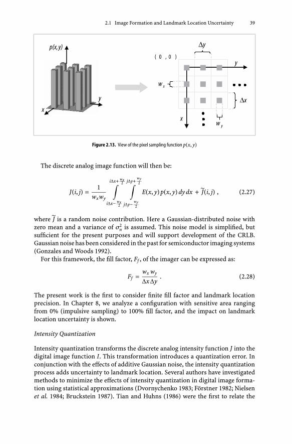
is the 2-D rectangle function centered on the coordinate (cx, cy) and with widthswx and wy in the x and y coordinate respectively. An illustration of the functionp(x, y) is shown in Figure 2.13.
2.1 Image Formation and Landmark Location Uncertainty 39
Figure 2.13. View of the pixel sampling function p(x, y)
The discrete analog image function will then be:
J(i, j) =1
wxwy
iΔx+ wx2∫
iΔx− wx2
jΔy+wy2∫
jΔy−wy2
E(x, y) p(x, y) dy dx + J(i, j) , (2.27)
where J is a random noise contribution. Here a Gaussian-distributed noise withzero mean and a variance of σ2
n is assumed. This noise model is simplified, butsufficient for the present purposes and will support development of the CRLB.Gaussian noise has been considered in the past for semiconductor imaging systems(Gonzales and Woods 1992).
For this framework, the fill factor, Ff , of the imager can be expressed as:
Ff =wx wy
Δx Δy. (2.28)
The present work is the first to consider finite fill factor and landmark locationprecision. In Chapter 8, we analyze a configuration with sensitive area rangingfrom 0% (impulsive sampling) to 100% fill factor, and the impact on landmarklocation uncertainty is shown.
Intensity Quantization
Intensity quantization transforms the discrete analog intensity function J into thedigital image function I. This transformation introduces a quantization error. Inconjunction with the effects of additive Gaussian noise, the intensity quantizationprocess adds uncertainty to landmark location. Several authors have investigatedmethods to minimize the effects of intensity quantization in digital image forma-tion using statistical approximations (Dvornychenko 1983; Förstner 1982; Nielsenet al. 1984; Bruckstein 1987). Tian and Huhns (1986) were the first to relate the
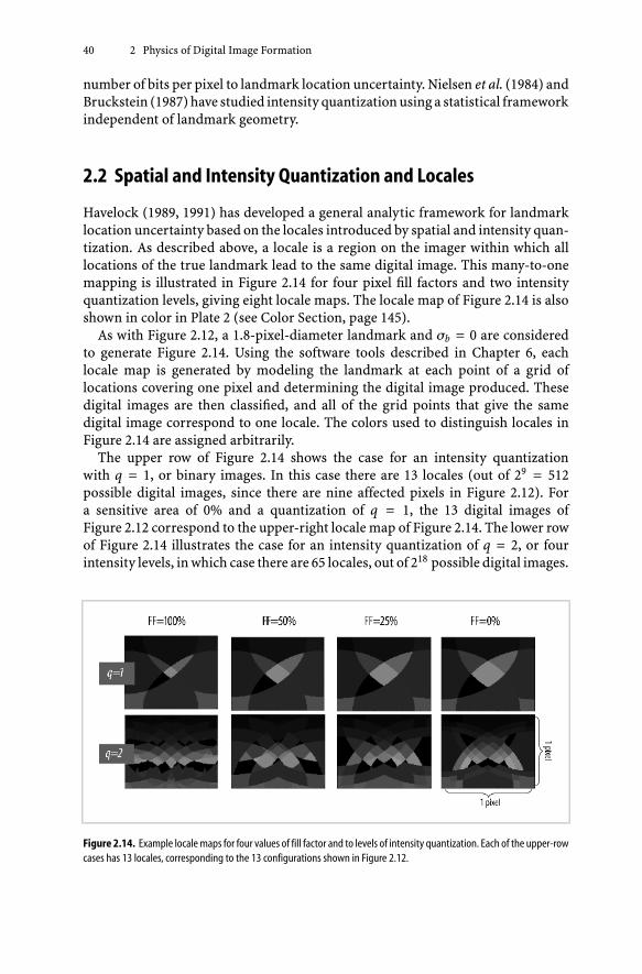
40 2 Physics of Digital Image Formation
number of bits per pixel to landmark location uncertainty. Nielsen et al. (1984) andBruckstein (1987) have studied intensity quantization using a statistical frameworkindependent of landmark geometry.
2.2 Spatial and Intensity Quantization and Locales
Havelock (1989, 1991) has developed a general analytic framework for landmarklocation uncertainty based on the locales introduced by spatial and intensity quan-tization. As described above, a locale is a region on the imager within which alllocations of the true landmark lead to the same digital image. This many-to-onemapping is illustrated in Figure 2.14 for four pixel fill factors and two intensityquantization levels, giving eight locale maps. The locale map of Figure 2.14 is alsoshown in color in Plate 2 (see Color Section, page 145).
As with Figure 2.12, a 1.8-pixel-diameter landmark and σb = 0 are consideredto generate Figure 2.14. Using the software tools described in Chapter 6, eachlocale map is generated by modeling the landmark at each point of a grid oflocations covering one pixel and determining the digital image produced. Thesedigital images are then classified, and all of the grid points that give the samedigital image correspond to one locale. The colors used to distinguish locales inFigure 2.14 are assigned arbitrarily.
The upper row of Figure 2.14 shows the case for an intensity quantizationwith q = 1, or binary images. In this case there are 13 locales (out of 29 = 512possible digital images, since there are nine affected pixels in Figure 2.12). Fora sensitive area of 0% and a quantization of q = 1, the 13 digital images ofFigure 2.12 correspond to the upper-right locale map of Figure 2.14. The lower rowof Figure 2.14 illustrates the case for an intensity quantization of q = 2, or fourintensity levels, in which case there are 65 locales, out of 218 possible digital images.
Figure 2.14. Example locale maps for four values of fill factor and to levels of intensity quantization. Each of the upper-rowcases has 13 locales, corresponding to the 13 configurations shown in Figure 2.12.

2.2 Spatial and Intensity Quantization and Locales 41
Four locale maps are shown in each row, corresponding to four levels of fillfactor. The changing shapes of the locales as one goes from 0% to 100% fill factorillustrates the impact of sensitive area on the detection of landmark location.
The size and shape of each locale corresponds to the distance the landmark mustbe displaced to change the digital image. As such, locale dimensions are indicativeof the local derivative of the analog intensity function with respect to location,(∂J/∂ pP∗
o
). A remarkable characteristic of locales is their irregularity, indicating
the nonstationary statistics of landmark location. In some regions of the image,a small shift of the landmark produces a change in the digital image, while in otherregions a large shift may not change the digital image.
The irregularity of the locales is also seen in the range of their aspect ratios;that is, the ratios of the longest to the shortest dimensions. For example, in thelower-right locale map, some locales are approximately isotropic, which is to saythey have an aspect ratio of approximately one, while others have a high aspectratio. The variability of locale aspect ratio also shows the variability of
(∂J/∂ pP∗
o
)as the true landmark location changes.
Practical situations, of course, involve larger landmarks and higher resolutionintensity quantization. Nonetheless, the essential features of locales carry over.The interaction of imager noise, J, and locales is considered in Section 3.2, wheresuitable analysis tools are developed.
With a larger landmark and more bits of intensity resolution there are morelocals, but irregularity remains a hallmark. For example, a study of a circularlandmark with a diameter of three pixels and a quantization of q = 4 gives 10,557locales. While the average area is 1/10,557 ∼ 10−4 pixels2, corresponding to hypo-thetical linear dimensions of 10−2 pixels, the actual largest locale has an area of0.0014 pixels2 and linear dimensions of 0.052 by 0.003 pixels, while the smallesthas an area of 1.5 × 10−11 pixels2 and linear dimensions of 9.1 × 10−6 by 4.3 × 10−6
pixels, or approximately 5 × 10³ smaller in linear dimensions than the largestlocale. These two locales have relatively low aspect ratios. Another locale of thestudy case has an aspect ratio of 8,000, measuring approximately 3.4 × 10−2 by4.3 × 10−6 pixels.
The properties of locales motivate two aspects of the treatment of landmarklocation uncertainty. The first is consideration of the true landmark location, pP∗
o , asa uniformly distributed random variable, distributed over an interval of ±1/2 pixel.The second is use of the 95% (or 99%) confidence interval to express uncertainty.
Considering locales, it is seen that the statistics of landmark location estimationdepend on precisely where the landmark falls on the imager. Since there is generallyno way to know precisely where the landmark center has fallen, the practicalapproach to uncertainty is to treat the true landmark location, pP∗
o , as a uniformlydistributed random variable. Because the statistics repeat with a shift of an integernumber of pixels, it is sufficient to study the statistics arising with a uniformdistribution on an area of one pixel, or from −1/2 to +1/2 pixel on each axis. The±1/2 pixel region, example locales, and repetition of the locales with a one-pixelshift are illustrated in Figure 2.15.

42 2 Physics of Digital Image Formation
Figure 2.15. Illustration of locales and ±1/2 pixel area of uniform probability distribution for pP∗o
A second aspect of the treatment of landmark location uncertainty is the properconsideration of estimator bias and covariance. Bias is defined as
pPbias0 = pP∗
o − pP∗0 , (2.29)
where pP∗o is the true landmark location, and
pP∗0 = T
(I∗) (2.30)
is the estimated location given by applying estimator T(·) to the noise-free digitalimage, I∗ (pP∗
o
). Actual imagers have noise, so that the measured digital image, I,
is a random variable. Treatment of the statistics of I follow in Section 3.2.2. Here,the important idea is that the ensemble of I with non-negligible probability givesa distribution of actual landmark location estimates that approximates pP∗
0 in themean and has a covariance given by
Σ = Cov pP0 = E{(pP0 − pP∗
0
)T (pP0 − pP∗0
)}. (2.31)
Approximating the distribution of pP0 with a 2-D Gaussian distribution, the com-bination of bias and covariance gives rise to a probability distribution that is offsetfrom pP∗
o and distributed over an elliptical region. This is illustrated in Figure 2.16,where the ellipse is drawn according to:
(pP0 − pP∗0
)T Σ−1 (pP0 − pP∗0
)= c , (2.32)
where c is a constant that is related by the χ2 distribution to the number of samplesexpected to lie inside the ellipse.
The bias and covariance matrix can be computed for a specified configurationand pP∗
o , but this is not directly useful, since these values vary rapidly over the

2.3 Illustrative Example 43
Figure 2.16. Illustration of estimator covariance and bias
±1/2 pixel area. In fact, when the landmark has two axes of symmetry, the averagebias is zero, as seen be the absence of a preferred direction. A method for repre-senting the uncertainty for this system with nonstationary statistics is required.The method chosen for this study is the circular 95% confidence interval. It is theradius of a circle centered on pP∗
o in which 95% of the estimates pP0 will fall, consid-ering, for each true landmark location pP∗
o , the bias and covariance illustrated inFigure 2.16, and also considering the uniform distribution of pP∗
o over the area ofone pixel. Computation of the confidence interval will require a four-dimensionalintegral. For each point pP∗
o , a 2-D integral over the Gaussian distribution of pP0
arising from pP∗o ; and then a 2-D integral over uniform distribution of pP∗
o over thearea of one pixel. Details of these integrals are the subject of Chapter 3.
2.3 Illustrative Example
We conclude this chapter with an illustrative example. On the one hand, theexample shows the use of a confidence interval and performance map; and onthe other, the impacts of sensitive area and diffraction smoothing are illustrated.The analysis was performed using a synthetic image of a landmark by startingwith the landmark geometrical description and applying the image formationtransformations indicated in Equation 2.4. For convenience, Figure 2.17 repeatsthese transformations, highlighting the user configuration parameters used.
Plate 3 (see Color Section, page 146) shows the distribution of
pP0 = pP0 − pP∗o (2.33)
for twelve cases, corresponding to three levels of fill factor, Ff = {0%, 50%, 100%}(shown with color in each subfigure), and to two values of smoothing parameter,σb =
{10−3, 5 × 10⁻³
}(in millimeters) on the imager, as well as to two values

44 2 Physics of Digital Image Formation
Figure 2.17. Configuration parameters for case study
of quantization resolution, q = {1, 8}. To visualize this figure, imagine that pP∗o
is the center for each of 100 samples. The points plotted then correspond topPo, and the confidence interval is the radius of the circle enclosing 95% of thesamples. The samples of pP∗
o are distributed randomly across the interval of ±1/2pixels. Landmark location pP0 has been estimated using the centroid estimator ofEquation 2.23 and Equation 2.24. This case study is made using the tools presentedin Chapter 6.
Plate 3 shows that use of grayscale information in the centroid algorithm canreduce uncertainty by 25% (we will see in Chapters 7 and 8 that model-basedestimators can give a sixfold improvement). Plate 3 also shows that an enlargedsensitive area can reduce uncertainty, particularly for a sharply focused image(σb = 0.001 mm). Finally, Plate 3 shows that increasing the image smoothing, forexample by defocusing the image, can improve landmark location precision.
In the next chapter the model developed in Section 2.1 and the methodologyoutlined in Section 2.2 are applied to determine the Cramér–Rao lower boundand also analysis tools for determining the uncertainty performance of practicalestimators.

3 Analytic Frameworkfor Landmark Location Uncertainty
In this chapter the mathematical tools for analyzing landmark location uncertaintyare developed. Two cases are considered. In Section 3.1 tools for calculating theCramér–Rao lower bound are developed, and in Section 3.2 tools are developed foranalyzing practical estimators. The two cases are quite different. The Cramér–Raolower bound assumes an unbiased estimator, and so the uncertainty is entirelydependent on the covariance component, determined by
(∂J/∂ pP∗
o
). Practical esti-
mators have bias that is dependent on the true landmark location, pP∗o . Interesting
challenges arise when performing the integration required, because the bias andcovariance can change so rapidly with pP∗
o .
3.1 Cramér–Rao Lower Bound
The Cramér–Rao lower bound methodology provides a theoretical statistical min-imum limit on the landmark location uncertainty and institutes a general frame-work for its study (Van Trees 1968). The ability to place a lower bound on landmarklocation uncertainty provides a benchmark for comparisons of the performanceof practical estimators and offers guidelines for the design of new estimators withimproved performance (Kay 1993).
The Cramér–Rao inequality has been widely used in statistical signal processingapplications. Some examples are the work of Reza and Doroodchi (1996), whoestablished the CRLB for the problem of detecting sudden changes in step-likesignals, Armstrong and Holeman (1998) in the determination of motion parameteruncertainty for Doppler radar tracking, and numerous efforts in the field of timedelay estimation in communication systems and sonar (Scharf 1990; Scharf andMcWhorter 1992). Applications of the CRLB in the field of image processing includethe work from Hung (1991), who determined the CRLB for the image restorationproblem, and also the framework developed by Robinson and Milanfar (2004), whoestablished the CRLB on the problem of interframe motion estimation in digitalimages.
A barrier to the development of the CRLB for landmark location uncertaintyis the difficulty involved in determining the spatial partial derivatives required,(∂J/∂ pP∗
o
). There are several obstacles to computing the spatial partial deriva-
tives. First, digital images are discontinuous functions of landmark location due to

46 3 Analytic Framework for Landmark Location Uncertainty
amplitude quantization. Second, when smoothing is considered, the illuminancefunction is not analytically tractable, making closed-form mathematical formu-lation of the spatial partial derivatives impossible and necessitating the use ofnumerical integration. The analog intensity function J and its derivatives must becomputed by numerical integration of the illuminance function, E(ix, iy), whichis performed by evaluating E(ix, iy) on a sample grid with a resolution of manypoints per pixel. Because the illuminance function is given by numerical convo-lution of the optical flux function with the smoothing operator, it is expensive tocompute; and integration of the confidence interval contributions over the ±1/2pixel distribution of pP∗
o requires that the integrations be performed many times,each with a slightly shifted landmark location. Previously known methods of 2-Dnumerical integration require the sample grid to be collocated with the region ofintegration (for details, see Figure 5.1). The use of an available method for 2-Dnumerical integration would require that the convolution be recomputed on a newsample grid for each position of the landmark evaluated, which would lead toprohibitively long computation times.
A second challenge is the nonstationarity of the statistics of pP0, or, equivalently,the strong dependence of
(∂J/∂ pP∗
o
)on the precise value of pP∗
o . Addressing thischallenge, several authors make use of the expected value of the CRLB over theevent space, creating a single-valued bound (e.g., Reza and Doroodchi 1996). Takinga different path, we use the confidence interval to characterize landmark locationuncertainty.
Considering these challenges, the strategy of this research comprises:
• Extensive modeling of image formation, including smoothing, which enablesthe numerical determination of the required spatial partial derivatives.
• Development of statistical confidence intervals based on the Cramér–Rao lowerbound. The bound will be calculated on the discrete analog amplitude function J.
• Development of a method of 2-D numerical integration that can be applied whenthe region of integration is not collocated with the sample grid.
These developments are described in Sections 3.1.1 and 3.1.2, and the integrationmethod is described in detail in Chapter 5.
3.1.1 Analytic Framework for Cramér–Rao Lower Bound
The derivation of the landmark location CRLB on the discrete analog intensityfunction J follows. The signal model for this problem is:
J(m, n, pP∗
o
)= J∗ (m, n, pP∗
o
)+ J(m, n) (3.1)
where J(m, n, pP∗
o
)is the discrete analog intensity function prior to quantization,
J∗ (m, n, pP∗o
)is the discrete analog intensity function, ideally produced by the
landmark at location pP∗o , and J(m, n) is a zero-mean white stationary Gaussian
process with variance, σ2n, and where m and n are indices on the pixel array.

3.1 Cramér–Rao Lower Bound 47
The joint likelihood function for the data J(m, n; pP∗o); n = 0, 1, 2, …, N − 1,
m = 0, 1, 2, …, M − 1; is related to the probability density function of J(m, n), andis given by:
p( J; pP∗o) =
∏m,n
1√2πσ2
n
e− (J(m,n,pP∗
o )−J∗(m,n;pP∗o ))2
2σ2n
=(2πσ2
n
)− mn2 e
− 12σ2
n
∑m,n
(J(m,n, pP∗
o )−J∗(m,n; pP∗o ))2
. (3.2)
The logarithm of the likelihood function is:
log p( J; pP∗o) = −
mn2
log(2πσ2
n
)−
12σ2
n
∑m,n
(J(m, n; pP∗
o) − J∗(m, n; pP∗o))2
. (3.3)
The Fisher information matrix (FIM) is given by:
[J(pP∗
o
)]i,j = −E
{∂2 log p( J; pP∗
o)∂ pP∗
i ∂ pP∗j
}, (3.4)
where E {•} is the expected value operator, i, j ∈ {1, 2} are indices on the two axes inimage coordinates, pP∗
0 = [pP∗1
pP∗2 ]
T is the true landmark location, and[J(
pP∗o
)]i,j is
the (i, j) element of the FIM. To determine the argument of the FIM in Equation 3.4,we proceed to establish the spatial partial derivative of Equation 3.3:
∂ log p( J; pP∗o)
∂ pP∗i
=1
σ2n
∑m,n
[(J(m, n; pP∗
o) − J∗(m, n; pP∗o)) ∂J∗(m, n; pP∗
o)∂ pP∗
i
]. (3.5)
From Equation 3.5, we get:
∂2 log p( J; pP∗o)
∂ pP∗i ∂ pP∗
j=
∂∂ pP∗
j
[∂ log p( J; pP∗
o)∂ pP∗
i
]
=1
σ2n
∂∂ pP∗
j
[∑m,n
[(J(m, n; pP∗
o) − J∗(m, n; pP∗o)) ∂J∗(m, n; pP∗
o)∂ pP∗
i
]]
=1
σ2n
[∑m,n
[(J(m, n; pP∗
o) − J∗(m, n; pP∗o)) ∂2J∗(m, n; pP∗
o)∂ pP∗
i ∂ pP∗j
−∂J∗(m, n; pP∗
o)∂ pP∗
i
∂J∗(m, n; pP∗o)
∂ pP∗j
]]. (3.6)
Substituting Equation 3.6 into Equation 3.4:
[J(pP∗
o
)]1,1 = −E
{∂2 log p(J; pP∗
o)
∂ pP∗1
2
}=
1σ2
n
∑m,n
(∂J∗(m, n; pP∗
o)∂ pP∗
1
)2
(3.7)
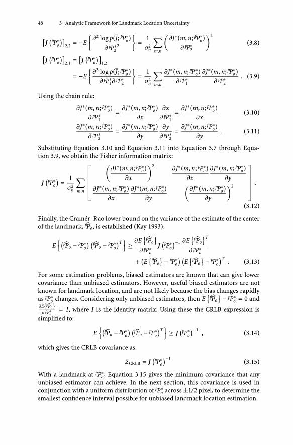
48 3 Analytic Framework for Landmark Location Uncertainty
[J(pP∗
o
)]2,2 = −E
{∂2 log p(J; pP∗
o)
∂ pP∗2
2
}=
1σ2
n
∑m,n
(∂J∗(m, n; pP∗
o)∂ pP∗
2
)2
(3.8)
[J(pP∗
o
)]2,1 =
[J(pP∗
o
)]1,2
= −E{
∂2 log p(J; pP∗o)
∂ pP∗1∂ pP∗
2
}=
1σ2
n
∑m,n
∂J∗(m, n; pP∗o)
∂ pP∗1
∂J∗(m, n; pP∗o)
∂ pP∗2
. (3.9)
Using the chain rule:
∂J∗(m, n; pP∗o)
∂ pP∗1
=∂J∗(m, n; pP∗
o)∂x
∂x∂ pP∗
1=
∂J∗(m, n; pP∗o)
∂x(3.10)
∂J∗(m, n; pP∗o)
∂ pP∗2
=∂J∗(m, n; pP∗
o)∂y
∂y∂ pP∗
2=
∂J∗(m, n; pP∗o)
∂y. (3.11)
Substituting Equation 3.10 and Equation 3.11 into Equation 3.7 through Equa-tion 3.9, we obtain the Fisher information matrix:
J(pP∗
o
)=
1σ2
n
∑m,n
⎡⎢⎢⎢⎣
(∂J∗(m, n; pP∗
o)∂x
)2 ∂J∗(m, n; pP∗o)
∂x∂J∗(m, n; pP∗
o)∂y
∂J∗(m, n; pP∗o)
∂x∂J∗(m, n; pP∗
o)∂y
(∂J∗(m, n; pP∗
o)∂y
)2
⎤⎥⎥⎥⎦ .
(3.12)
Finally, the Cramér–Rao lower bound on the variance of the estimate of the centerof the landmark, pPo, is established (Kay 1993):
E{(pPo − pP∗
o
) (pPo − pP∗o
)T}
≥ ∂E{
pPo}
∂ pP∗o
J(pP∗
o
)−1 ∂E{
pPo}T
∂ pP∗o
+(E{pPo
}− pP∗
o
) (E{pPo
}− pP∗
o
)T. (3.13)
For some estimation problems, biased estimators are known that can give lowercovariance than unbiased estimators. However, useful biased estimators are notknown for landmark location, and are not likely because the bias changes rapidlyas pP∗
o changes. Considering only unbiased estimators, then E{
pPo}
− pP∗o = 0 and
∂E{pPo}∂ pP∗
o= I, where I is the identity matrix. Using these the CRLB expression is
simplified to:
E{(pPo − pP∗
o
) (pPo − pP∗o
)T}
≥ J(pP∗
o
)−1, (3.14)
which gives the CRLB covariance as:
ΣCRLB = J(pP∗
o
)−1(3.15)
With a landmark at pP∗o , Equation 3.15 gives the minimum covariance that any
unbiased estimator can achieve. In the next section, this covariance is used inconjunction with a uniform distribution of pP∗
o across ±1/2 pixel, to determine thesmallest confidence interval possible for unbiased landmark location estimation.

3.1 Cramér–Rao Lower Bound 49
3.1.2 CRLB Confidence Interval
Figure 3.1 illustrates the CRLB covariance uncertainty contours at nine positionsinside the ±0.1 pixel area of a hypothetical configuration. The nine ellipses of Fig-ure 3.1 represent the 95% confidence intervals for the covariance of a given estimatepPo (shown with a dot) of a true center pP∗
o (shown with a cross). A 4-D integrationis required to form the confidence interval. At each point pP∗
o , a 2-D integrationof the Gaussian-distributed probability density function for pPo is required to getthe confidence interval contribution at pP∗
o (Equation 3.16, below), and then a 2-Dintegration across the uniformly distributed probability density function for pP∗
o(Equation 3.20, below).
The CRLB cumulative probability function for an estimate pPo, at a distance Rfrom pP∗
o is defined as:
FCRLBpPo
{R; pP∗
o
}= p
(∥∥pPo − pP∗o
∥∥ < R)
=
R∫
r=0
2π∫
α=0
rG(pP; pP∗o , ΣCRLB) dα dr , (3.16)
where G(
pP; pP∗o , ΣCRLB
)is a Gaussian probability function centered on pP∗
o andcovariance ΣCRLB:
G(pP, pP∗
o
)=
1
2π√|ΣCRLB| e− 1
2(pP−pP∗
o)T Σ−1
CRLB(pP−pP∗
o)
, (3.17)
where |ΣCRLB| is the determinant of the CRLB covariance matrix.
Figure 3.1. CRLB uncertainty contours at different position estimates
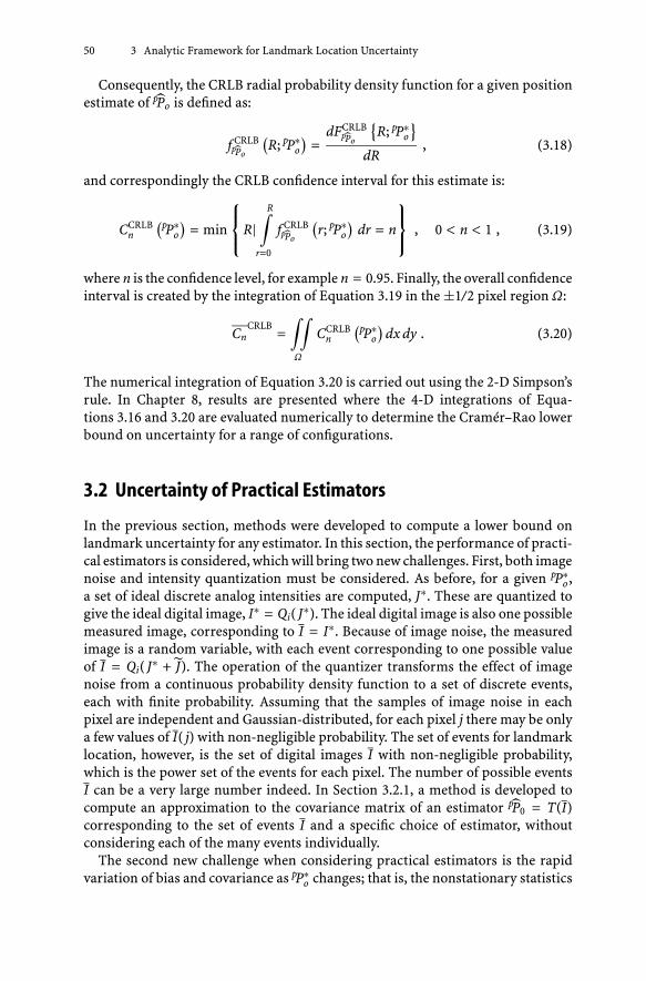
50 3 Analytic Framework for Landmark Location Uncertainty
Consequently, the CRLB radial probability density function for a given positionestimate of pPo is defined as:
f CRLBpPo
(R; pP∗
o
)=
dFCRLBpPo
{R; pP∗
o
}
dR, (3.18)
and correspondingly the CRLB confidence interval for this estimate is:
CCRLBn
(pP∗o
)= min
⎧⎨⎩R|
R∫
r=0
f CRLBpPo
(r; pP∗
o
)dr = n
⎫⎬⎭ , 0 < n < 1 , (3.19)
where n is the confidence level, for example n = 0.95. Finally, the overall confidenceinterval is created by the integration of Equation 3.19 in the ±1/2 pixel region Ω:
CnCRLB
=∫∫
Ω
CCRLBn
(pP∗o
)dx dy . (3.20)
The numerical integration of Equation 3.20 is carried out using the 2-D Simpson’srule. In Chapter 8, results are presented where the 4-D integrations of Equa-tions 3.16 and 3.20 are evaluated numerically to determine the Cramér–Rao lowerbound on uncertainty for a range of configurations.
3.2 Uncertainty of Practical Estimators
In the previous section, methods were developed to compute a lower bound onlandmark uncertainty for any estimator. In this section, the performance of practi-cal estimators is considered, which will bring two new challenges. First, both imagenoise and intensity quantization must be considered. As before, for a given pP∗
o ,a set of ideal discrete analog intensities are computed, J∗. These are quantized togive the ideal digital image, I∗ = Qi( J∗). The ideal digital image is also one possiblemeasured image, corresponding to I = I∗. Because of image noise, the measuredimage is a random variable, with each event corresponding to one possible valueof I = Qi( J∗ + J). The operation of the quantizer transforms the effect of imagenoise from a continuous probability density function to a set of discrete events,each with finite probability. Assuming that the samples of image noise in eachpixel are independent and Gaussian-distributed, for each pixel j there may be onlya few values of I( j) with non-negligible probability. The set of events for landmarklocation, however, is the set of digital images I with non-negligible probability,which is the power set of the events for each pixel. The number of possible eventsI can be a very large number indeed. In Section 3.2.1, a method is developed tocompute an approximation to the covariance matrix of an estimator pP0 = T(I)corresponding to the set of events I and a specific choice of estimator, withoutconsidering each of the many events individually.
The second new challenge when considering practical estimators is the rapidvariation of bias and covariance as pP∗
o changes; that is, the nonstationary statistics

3.2 Uncertainty of Practical Estimators 51
of pP0. Two-dimensional numerical integration operates by fitting a polynomialsurface to values of the integrand and forming the definite integral of the poly-nomial surface. The correctness of this approach depends on the integrand beingsufficiently smooth, which is not the case for the bias and covariance of landmarklocation estimators. To avoid aliasing and other errors that might arise with aninteraction between a regular sampling grid and the underlying and unknownstructure of locales, Monte Carlo integration is used for the 2-D integration ofthe uniform distribution of pP∗
o over ±1/2 pixels (McCluer 2000). Monte Carlointegration has rather slow convergence, and so the numerically computed errordistributions are somewhat rough for practical computing times, but the methodavoids systematic errors. Recall that a 4-D integration is required to compute thedistribution of pPo, a 2-D integration over the biased, Gaussian ellipse correspond-ing to a specific pP∗
o , and then a 2-D integration is necessary over the uniformdistribution of pP∗
o across ±1/2 pixel. The integrand of the first 2-D integration issmooth and can be integrated by standard techniques, in this case the 2-D Simp-son’s rule. The latter is addressed by Monte Carlo integration. These methods arederived in Section 3.2.2.
3.2.1 Analytic Framework for Practical Estimators
In the absence of noise, the digital image is created from the amplitude quantizationof the discrete analog intensity function:
I∗ = Qi( J∗) , (3.21)
where J∗ is a column vector of Np analog intensity values corresponding to the Np
pixels comprising the image of the landmark. In the presence of noise, the digitalimage is expressed as:
I = Qi( J∗ + J) = Qi( J) , (3.22)
where J is Gaussian noise with variance σ2n. There is a finite set of digital images, and
in principle the covariance of θ can be determined by forming θ and the probabilityassociated with each one. However, with even a moderate level of imager noise J,there are an enormous number of possible digital images of the landmark, and soan efficient method of computing the covariance matrix is needed. This is done byTaylor series expansion of the covariance matrix itself.
For each pixel j, there is a finite set of events I( j) induced by the image noise Joperating through the quantizer. The event i of pixel j is indexed by ij, so I( j, ij) isa specific possible quantized value for pixel j. By restricting our attention to eventswith probabilities that are greater than some threshold, such as p(I( j, ij)) > 10−6,a number M(j) of events for pixel j need to be considered. For example, consideringa hypothetical pixel j with eight-bit quantization, an ideal analog intensity value ofJ∗( j) = 121.3 (in ADC counts) and a noise figure of σn = 0.6 (in counts). Then thenoise-free quantized intensity value is I∗ = 121, and the values ij and probabilitiesfor several possible events of pixel j are shown in Table 3.1. Notice that the eventindex ij is arranged such that I( j, ij) = I∗( j) + ij.

52 3 Analytic Framework for Landmark Location Uncertainty
Table 3.1. Example data showing enumeration of events for pixel j with J∗ = 121.3 and σn = 0.6. Events withp(I( j, ij)
)> 10−6 are shown. M( j) = 6 for the example pixel.
Range of analog intensity Event index ij I(j, ij
)p(I(j, ij
))
118.5 < J ≤ 119.5 −2 119 0.001348119.5 < J ≤ 120.5 −1 120 0.089861120.5 < J ≤ 121.5 0 121 0.539347121.5 < J ≤ 122.5 1 122 0.346671122.5 < J ≤ 123.5 2 123 0.022627123.5 < J ≤ 124.5 3 124 0.000123
Let M denote the total number of digital images, Ik, k = 1, …, M, that can beformed by the joint event {i1, i2, i3, …, iN}; that is, the total set of images is thepower set of possible pixel intensity values:
M =Np∏j=1
M( j) (3.23)
Index k is then an index on the power set. Each k is associated with a joint eventwith particular values for each of {i1, i2, i3, …, iN}.
From here it is possible to define the covariance of the landmark location esti-mator as:
Cov θ = E{
θθT} =∑
i1
∑i2
∑i3
· · ·∑
iN
Pi1 Pi2 Pi3 · · · PiN
(θkθT
k
), (3.24)
where each summation is over the M( j) events of pixel j, Pij is a shorthand notationfor the probability p(I( j, ij)), and the misadjustment of the landmark locationestimate θk, corresponding to Ik, is given by:
θk = θ{i1,i2,i3,…,iN } = θI∗ − θk
= T(I∗) − T(Ik) , (3.25)
where T(I) is the output of a landmark location estimator applied to image I.Equation 3.24 is not usable in practice given the large power set M. For example,a 10×10 image where each pixel has six possible outcomes will generate 6100 digitalimages!
Rather than enumerating the large power set of possible digital images, thecovariance of θ is formed using the Taylor series expansion. A particular digitalimage Ik (caused by the joint event {i1, i2, i3, …, iN}) can be expressed as:
Ik = I∗ + ∂Ik , (3.26)
where
δIk = [i1i2i3 · · · iN ]T . (3.27)

3.2 Uncertainty of Practical Estimators 53
The estimator output is given by the Taylor series expansion:
T(Ik)
= θk = θ{i1,i2,i3,…,iN } = θI∗ +∂T∂I
∣∣∣∣I=I∗
δIk + O(
12
∂2T∂Ij1 ∂Ij2
δIj1 δIj2
)(3.28)
= θI∗ +
Np∑j=1
∂T∂Ij
∣∣∣∣I=I∗
δIkj + O
(12
∂2T∂Ij1 ∂Ij2
δIj1 δIj2
)z .
Keeping the first term:
⇒ T(Ik) ∼= θI∗ +
(δθi1 + δθi2 + δθi3 · · · + δθiN
), (3.29)
where
δθj =∂T∂Ij
∣∣∣∣I=I∗
δIkj . (3.30)
That is, δθj is the change in the landmark location estimate due to a change in thequantized value for pixel j. Using Equations 3.25 and 3.26, θk can be written as:
θk = θ{i1,i2,i3,…,iN } = T(I∗) − T(Ik) = θI∗ − θk
=(
θI∗ − θI∗ −∂T∂I
∣∣∣∣I=I∗
δIk)
=(
θI∗ −∂T∂I
∣∣∣∣I=I∗
δIk)
=[θI∗ −
(δθi1 + δθi2 + δθi3 · · · + δθiN
)]. (3.31)
Working in error coordinates, Equation 3.31 can be written as:
θk = θ{i1,i2,i3,…,iN } =(δθi1 + δθi2 + δθi3 · · · + δθiN
). (3.32)
Substituting Equation 3.32 into Equation 3.24, we get:
E{
θθT} (3.33)
=M(1)∑i1=1
M(2)∑i2=1
M(3)∑i3=1
· · ·M(N)∑iN =1
Pi1 Pi2 Pi3 · · ·PiN
(δθi1 δθi2 δθi3 · · · δθiN
)(δθi1 δθi2 δθi3 · · · δθiN
)T.
Equation 3.33 is the linear covariance approximation desired. Note that this for-mulation has linear computational complexity. This equation can be implementedby recursive induction, as follows:
Let’s define the covariance by considering the first pixel as:
C1 =M(1)∑i1=1
Pi1 δθi1 δθTi1 , (3.34)

54 3 Analytic Framework for Landmark Location Uncertainty
which means that the covariance C2 due to the contributions of pixels 1 and 2 is:
C2 =M(1)∑i1=1
M(2)∑i2=1
Pi1 Pi2
(δθi1 + δθi2
) (δθi1 + δθi2
)T
=M(1)∑i1=1
Pi1
M(2)∑i2=1
Pi2
(δθi1 δθT
i1 + δθi1 δθTi2 + δθi2 δθT
i1 + δθi2 δθTi2
)(3.35)
=M(1)∑i1=1
Pi1 δθi1 δθTi1 +
M(1)∑i1=1
Pi1
M(2)∑i2=1
Pi2
(δθi1 δθT
i2 + δθi2 δθTi1
)+
M(1)∑i1=1
Pi1
M(2)∑i2=1
Pi2 δθi2 δθTi2
=M(1)∑i1=1
Pi1 δθi1 δθTi1 +
M(1)∑i1=1
Pi1 δθi1
M(2)∑i2=1
Pi2 δθTi2 +
M(2)∑i2=1
Pi2 δθi2
M(1)∑i1=1
Pi1 δθTi1 +
M(2)∑i2=1
Pi2 δθi2 δθTi2 ,
which in turn can be expressed as
C2 = C1 + E{
θi1
}E{
θTi2
}+ E
{θi2
}E{
θTi1
}+
M(2)∑i2=1
Pi2 δθi2 δθTi2 . (3.36)
Finally, by induction, the covariance CN due to the contributions of pixels 1, …, Ncan be calculated from the covariance CN−1:
CN = E{
Cov θ}
= CN−1 + E{
δθi1 + δθi2 + · · · + δθiN−1
}E{
δθTiN
}
+ E{
δθiN
}E{(
δθi1 + δθi2 + · · · + δθiN−1
)T}
+M(N)∑iN =1
PiN δθiN δθTiN , (3.37)
where CN is the covariance of the landmark location estimate pPo, considering theuncertainty introduced by pixels 1, …, N, and considering intensity quantization.
3.2.2 Landmark Location Estimator Confidence Interval
The procedure used to compute the landmark location estimator confidence inter-val is slightly different to the one used to compute the CRLB confidence interval.Practical estimators exhibit bias; that is, the expected value of the estimate is notequal to the real location of the image of the center of the landmark. Furthermore,in general these biases are not constant. This bias must be considered to determinethe landmark location estimator confidence interval.
Figure 3.2 illustrates the bias and covariance computed at seven points fora particular landmark and estimator. The figure is made in this way, as each ofseven points pP∗
o , shown as crosses in the figure, the landmark mark is simulated,

3.2 Uncertainty of Practical Estimators 55
Figure 3.2. Estimator uncertainty contours at different positions estimates
the illuminance function is generated and J∗ is computed. This is passed to theestimator, which gives:
pP∗o = Tc
(I∗) , (3.38)
where Tc( ) is the binary image centroid estimator. The vectors in Figure 3.2 showthe bias. Notice that the bias is zero when pP∗
o falls at the center of the pixel. Finallyan ellipse is drawn according to
(pPo − pP∗o
)T Σ−1 (pPo − pP∗o
)= 5.99 , (3.39)
where Σ = CN is the covariance matrix computed, and χ2 = 5.99 corresponds tothe 95% confidence interval when two parameters are estimated.
The estimator uncertainty cumulative probability function at a distance R frompP∗
o is defined as:
FTpPo
{R; E
{pP∗o
}− pPo
}= p
(∥∥pPo − pP∗o
∥∥ < R)
=
R∫
r=0
2π∫
α=0
rG(pP; E
{pPo}
− pP∗o , ΣT
)dα dr , (3.40)
where G(
pP; pP∗o , ΣCRLB
)is a Gaussian probability function centered on E
{pPo
}− pP∗
oand covariance ΣT :
G(pP
)=
1
2π√|ΣT| e− 1
2(pP−E{pPo}+ pP∗
o)T Σ−1
T(pP−E{pPo}+ pP∗
o)
, (3.41)
where |ΣT| is the determinant of covariance matrix ΣT . Consequently, the estimatoruncertainty radial probability density function for a given position estimate pP∗
o isdefined as (Peebles 2001):

56 3 Analytic Framework for Landmark Location Uncertainty
fpPo
(R; E
{pP∗o
}− pPo
)=
dFpPo
{R; E
{pP∗
o
}− pPo
}dR
, (3.42)
and correspondingly the estimator confidence interval for this estimate is:
Cn(pP∗
o
)= min
⎧⎨⎩R|
R∫
r=0
fpPo
(r; E
{pP∗o
}− pPo
)dr = n
⎫⎬⎭ , 0 < n ≤ 1 , (3.43)
where n reflects the confidence level (e.g., n = 95% or n = 99%), and Cn is theradius of a circle within which pP will lie in the fraction n of cases.
Finally, the overall confidence interval is created by the integration of Equa-tion 3.43 in the ±1/2 pixel region Ω:
Cn =∫∫
Ω
Cn(pP∗
o
)dx dy . (3.44)
Monte Carlo integration is used to evaluate Equation 3.44, to overcome the chal-lenge of a rapidly varying integrand. In Chapter 8, results are presented where the3-D integrations of Equations 3.43 and 3.44 are evaluated numerically to determinethe Cramér–Rao lower bound on uncertainty for a range of configurations.
3.3 Discussion
The methods developed here employ a mix of analytic results where tractable andnumerical methods where necessary. Using these tools, the Cramér–Rao lowerbound can be computed for a given landmark and imager configuration, inde-pendent of the estimator used , and the uncertainty of practical estimators canbe determined. This chapter, and indeed this entire work, has focused on circu-lar landmarks, but with suitable extension of the methods, the analysis can beapplied to arbitrary landmark shapes. The calculation of
(∂J/∂ pP∗
o
), for example,
is achieved by integrating the illuminance along the edges of the sensitive areas,which can be done whenever the illuminance function can be formed.
In the next chapter, two model-based landmark location estimators are devel-oped. Following that, in Chapters 5 and 6, the mechanics for implementing theresults of this chapter are laid out. This is then followed, in Chapter 8, by theanalysis of a circular landmark and practical estimators.
4 Model-based Landmark Location Estimators
The most important feature and information-rich portion of a landmark is itsedge. The landmark edge is smoothed by both the finite sensitive area of the pixeland the illuminance function. The illuminance function of a circular landmark,rendered in a 3-D plot such as Plate 4 (see Color Section, page 147), has the lookof a tepuy1 or table mountain.
Two model-based landmark location estimators are presented here. These esti-mators reduce bias by explicitly modeling the illuminance function given by thelandmark, and they reduce uncertainty by exploiting the intermediate grayscalevalues given by smoothing at the edge of the landmark. These algorithms are in-spired, in part, by the Nalwa–Binford algorithm for precise edge location (Nalwaand Binford 1986). This algorithm locates a line-edge by modeling the smoothtransition between light on one side and dark on the other.
The ellipsoidal contour algorithm, described in Section 4.1, operates by fittingan ellipse to points produced by the contour routine in MATLAB®. Interior andexterior intensities are first detected, so that the contour level can be selected as themean intensity. This corresponds approximately to the midway point of the tran-sition between the interior and exterior of the landmark. The ellipsoidal contourmodel has five parameters, corresponding to an ellipse center, pP0, radius, eccen-tricity, and orientation. The algorithm was first developed to seed the parametervalues for the more complex Butterworth tepuy algorithm; but to our surprise itgave an analytic and experimental performance indistinguishable from the morecomplex algorithm. An explanation for this is considered after the estimators arepresented.
The Butterworth tepuy algorithm, described in Section 4.2, was developed tocapture a parametric model of the illuminance of a circular landmark that canbe fit to the measured digital image. The fit can be carried out with, for example,the Newton–Raphson method. The model is parametric in the sense that it isexpressed in closed form. While it captures the width of the transition region asa parameter, just like the Nalwa–Binford algorithm, the model does not rely onnumerical values for pixel sensitive area or smoothing radius.
As will be shown through both analysis and experiment, the two model-basedestimators significantly reduce landmark location uncertainty. Indeed, they oper-
1 Tepuy means “table mountain” in the native language of the Pemon tribes located in the GranSabana, Venezuela.
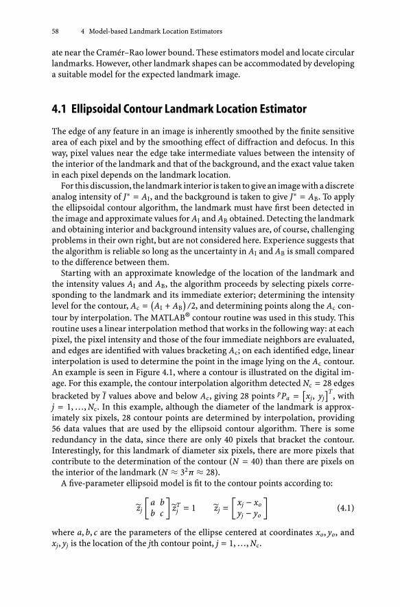
58 4 Model-based Landmark Location Estimators
ate near the Cramér–Rao lower bound. These estimators model and locate circularlandmarks. However, other landmark shapes can be accommodated by developinga suitable model for the expected landmark image.
4.1 Ellipsoidal Contour Landmark Location Estimator
The edge of any feature in an image is inherently smoothed by the finite sensitivearea of each pixel and by the smoothing effect of diffraction and defocus. In thisway, pixel values near the edge take intermediate values between the intensity ofthe interior of the landmark and that of the background, and the exact value takenin each pixel depends on the landmark location.
For this discussion, the landmark interior is taken to give an image with a discreteanalog intensity of J∗ = AI, and the background is taken to give J∗ = AB. To applythe ellipsoidal contour algorithm, the landmark must have first been detected inthe image and approximate values for AI and AB obtained. Detecting the landmarkand obtaining interior and background intensity values are, of course, challengingproblems in their own right, but are not considered here. Experience suggests thatthe algorithm is reliable so long as the uncertainty in AI and AB is small comparedto the difference between them.
Starting with an approximate knowledge of the location of the landmark andthe intensity values AI and AB, the algorithm proceeds by selecting pixels corre-sponding to the landmark and its immediate exterior; determining the intensitylevel for the contour, Ac =
(AI + AB
)/2, and determining points along the Ac con-
tour by interpolation. The MATLAB® contour routine was used in this study. Thisroutine uses a linear interpolation method that works in the following way: at eachpixel, the pixel intensity and those of the four immediate neighbors are evaluated,and edges are identified with values bracketing Ac; on each identified edge, linearinterpolation is used to determine the point in the image lying on the Ac contour.An example is seen in Figure 4.1, where a contour is illustrated on the digital im-age. For this example, the contour interpolation algorithm detected Nc = 28 edgesbracketed by I values above and below Ac, giving 28 points pPa =
[xj, yj
]T, with
j = 1, …, Nc. In this example, although the diameter of the landmark is approx-imately six pixels, 28 contour points are determined by interpolation, providing56 data values that are used by the ellipsoid contour algorithm. There is someredundancy in the data, since there are only 40 pixels that bracket the contour.Interestingly, for this landmark of diameter six pixels, there are more pixels thatcontribute to the determination of the contour (N = 40) than there are pixels onthe interior of the landmark (N ≈ 32π ≈ 28).
A five-parameter ellipsoid model is fit to the contour points according to:
zj
[a bb c
]zT
j = 1 zj =[
xj − xo
yj − yo
](4.1)
where a, b, c are the parameters of the ellipse centered at coordinates xo, yo, andxj, yj is the location of the jth contour point, j = 1, …, Nc.

4.1 Ellipsoidal Contour Landmark Location Estimator 59
Figure 4.1. Example of ellipsoidal contour around a landmark. Subplot b shows the illuminance function of the image ofthe landmark. Subplot a shows the corresponding digital image and contour fit to the data.
A nonlinear least squares estimation for parameters θ = [a, b, c, xo, yo]T is donefor this model, using the Newton–Raphson method. As a nonlinear estimation tech-nique, the Newton–Raphson algorithm requires initial parameter values, whichshould be as close as is practical to the true values. In principle the algorithm canfail if the initial, or “seed,” values are too far from the true solution, but in this casesuitable initial parameters are easily determined:
• Seed values for xo, yo are determined by applying the centroid algorithm to thelandmark;
• A linear fit is used to find seed values for the ellipsoid parameters a, b, c byevaluating the 3 × Nc system of equations:
1 = [a b c]
⎡⎣
(xj − x0
)2(xj − x0
) (yj − y0
)(
yj − y0)2
⎤⎦ . (4.2)
Once the seed values are determined, the Newton–Raphson algorithm is run tominimize the error:
ε =Nc∑j=1
(zj
[a bb c
]zT
j − 1)2
; zj =[
xj − xo
yj − yo
]. (4.3)
The estimate for the center of the image of the landmark is taken directly from thefitted parameters xo, yo. Figure 4.1 shows a contour established on the digital imageof a circular landmark (a) from the illuminance function displayed in (b). The
points zj =[
xj − xo
yj − yo
]correspond to pixels that belong to the contour established.

60 4 Model-based Landmark Location Estimators
4.2 Butterworth Tepuy Landmark Location Estimator
This model-based estimator is inspired by the shape of a tepuy or table mountain,as it models the 3-D shape of the illuminance function that corresponds to a circularlandmark. As described in Chapter 2, the diffraction phenomenon is modeled asthe convolution of the optical flux function H(x, y) and a 2-D Gaussian kernel toproduce the illuminance function E(x, y). The result of convolving the Gaussiankernel with a circular landmark will be called a Gaussian tepuy (see Plate 5, part a,in the Color Section, page 148).
The closed-form equation of the Gaussian tepuy does not exist; for this reasonit is necessary to approximate its mathematical formulation with another func-tion (Proakis and Manolakis 1996). A suitable approximation is the expressionof the frequency magnitude of a 2-D Butterworth filter, scaled appropriately. Theexpression of the Butterworth tepuy is:
E(x, y) ≈ EBT(x, y; a, b, c, xo, yo, Lmax, Lmin, sb
)
=Lmax − Lmin
1 +
((x − xo
)2+(
y − yo)2
R(x, y)2
) R(x,y)sb
+ Lmin , (4.4)
where E(x, y) is the true illuminance function, EBT(·) is the Butterworth tepuymodel, and R(x, y) is the radius of an ellipse along the vector V = [(x−xo), (y−yo)],defined as:
R(x, y) = R(x, y; a, b, c, xo, yo) =
√√√√√√√√√√
(x − xo
)2
(y − yo
)2 + 1
a
(x − xo
)2
(y − yo
)2 + 2b
(x − xo
)(
y − yo) + c
. (4.5)
Plate 5 shows a comparison between a circular landmark smoothed by a Gaussiandiffraction kernel with variance σ2
b and a Butterworth tepuy.
Figure 4.2. Ellipsoidal radius
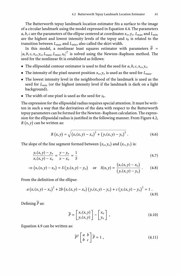
4.2 Butterworth Tepuy Landmark Location Estimator 61
The Butterworth tepuy landmark location estimator fits a surface to the imageof a circular landmark using the model expressed in Equation 4.4. The parametersa, b, c are the parameters of the ellipse centered at coordinates xo, yo. Lmax and Lmin
are the highest and lowest intensity levels of the tepuy and sb is related to thetransition between Lmax and Lmin, also called the skirt width.
In this model, a nonlinear least squares estimator with parameters θ =[a, b, c, xo, yo, Lmax, Lmin, sb]
T is solved using the Newton–Raphson method. Theseed for the nonlinear fit is established as follows:
• The ellipsoidal contour estimator is used to find the seed for a, b, c, xo, yo.
• The intensity of the pixel nearest position xo, yo is used as the seed for Lmax.
• The lowest intensity level in the neighborhood of the landmark is used as theseed for Lmin (or the highest intensity level if the landmark is dark on a lightbackground).
• The width of one pixel is used as the seed for sb.
The expression for the ellipsoidal radius requires special attention. It must be writ-ten in such a way that the derivatives of the data with respect to the Butterworthtepuy parameters can be formed for the Newton–Raphson calculation. The expres-sion for the ellipsoidal radius is justified in the following manner. From Figure 4.2,R(x, y
)can be written as:
R(x, y
)=√(
xr(x, y) − xo)2
+(
yr(x, y) − yo)2
. (4.6)
The slope of the line segment formed between(xo, yo
)and
(xr, yr
)is:
yr(x, y) − yo
xr(x, y) − xo=
y − yo
x − xo=
1S
(4.7)
⇒ (xr(x, y) − xo
)= S
(yr(x, y) − yo
)or S(x, y) =
(xr(x, y) − xo
)(
yr(x, y) − yo) . (4.8)
From the definition of the ellipse:
a(xr(x, y) − xo
)2+ 2b
(xr(x, y) − xo
) (yr(x, y) − yo
)+ c
(yr(x, y) − yo
)2 = 1 .(4.9)
Defining P as:
P =[
xr(x, y)yr(x, y)
]−[
xo
yo
], (4.10)
Equation 4.9 can be written as:
PT[
a bb c
]P = 1 , (4.11)

62 4 Model-based Landmark Location Estimators
or equivalently
PTQP =∥∥P∥∥
Q = 1 , (4.12)
where
Q =[
a bb c
]. (4.13)
Substituting Equation 4.8 into Equation 4.9, we get
aS2 (yr(x, y) − yo)2
+ 2bS(
yr(x, y) − yo)2
+ c(
yr(x, y) − yo)2 = 1
⇒ (yr(x, y) − yo
)2 =1
aS2 + 2bS + c. (4.14)
From Equations 4.8 and 4.14:
⇒ (xr(x, y) − xo
)2 =S2
aS2 + 2bS + c. (4.15)
Substituting Equations 4.14 and 4.15 into Equation 4.6, we get:
R(x, y) =
√S(x, y)2
aS(x, y)2 + 2bS(x, y) + c+
1aS(x, y)2 + 2bS(x, y) + c
. (4.16)
Finally, substituting Equation 4.8 into Equation 4.16, we obtain:
R(x, y) = R(x, y; a, b, c, xo, yo) =
√√√√√√√√√√
(x − xo
)2
(y − yo
)2 + 1
a
(x − xo
)2
(y − yo
)2 + 2b
(x − xo
)(
y − yo) + c
. (4.17)
Equation 4.17 can be expressed in a more compact form:
R(x, y) = R(x, y; a, b, c, xo, yo) =
√√√√(x − xo
)2+(
y − yo)2
a(x − xo
)2+ 2b
(x − xo
) (y − yo
)+ c
(y − yo
)2
=√
‖P‖2/‖P‖2Q (4.18)
or
R(x, y) = R(x, y; a, b, c, xo, yo) = ‖P‖/‖P‖Q . (4.19)

4.3 Discussion 63
Using Equation 4.19, the expression for the Butterworth tepuy, Equation 4.4, canbe further simplified by substitution:
EBT(x, y; a, b, c, xo, yo, Lmax, Lmin, sb) =Lmax − Lmin
1 +(∥∥P
∥∥2Q
)‖P‖/‖P‖Qsb
+ Lmin . (4.20)
Using Equation 4.20, the parameters of the Butterworth tepuy model are fit byusing the Newton–Raphson method to minimize
ε =Np∑j=1
(I( j) − EBT(θ)
)2, (4.21)
where θ = [a, b, c, xo, yo, Lmax, Lmin, sb]T is the parameter vector, j is the pixel index,
and Np is the number of pixels used for the estimation. The estimate for thecenter of the image of the landmark is taken directly from the fitted parameters,
pPoL
=[
xo
yo
].
4.3 Discussion
Two model-based estimators have been presented. They operate very differently.The ellipsoidal contour algorithm fits the parameters of an ellipse to contour pointsobtained by interpolating the pixel data. The Butterworth tepuy algorithm fits theintensity data directly. In spite of these differences and a significant differencein computational cost (with the ellipsoidal contour being the faster to compute),the two model-based estimators show closely comparable performance. In whatfollows, these location estimators will be evaluated with the analysis methodsderived in Chapter 3 using the tools described in Chapter 6. The location estimatorswill also be tested with the experiment described in Chapter 7.
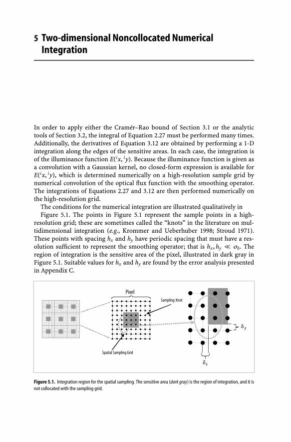
5 Two-dimensional Noncollocated NumericalIntegration
In order to apply either the Cramér–Rao bound of Section 3.1 or the analytictools of Section 3.2, the integral of Equation 2.27 must be performed many times.Additionally, the derivatives of Equation 3.12 are obtained by performing a 1-Dintegration along the edges of the sensitive areas. In each case, the integration isof the illuminance function E(ix, iy). Because the illuminance function is given asa convolution with a Gaussian kernel, no closed-form expression is available forE(ix, iy), which is determined numerically on a high-resolution sample grid bynumerical convolution of the optical flux function with the smoothing operator.The integrations of Equations 2.27 and 3.12 are then performed numerically onthe high-resolution grid.
The conditions for the numerical integration are illustrated qualitatively inFigure 5.1. The points in Figure 5.1 represent the sample points in a high-
resolution grid; these are sometimes called the “knots” in the literature on mul-tidimensional integration (e.g., Krommer and Ueberhuber 1998; Stroud 1971).These points with spacing hx and hy have periodic spacing that must have a res-olution sufficient to represent the smoothing operator; that is hx, hy << σb. Theregion of integration is the sensitive area of the pixel, illustrated in dark gray inFigure 5.1. Suitable values for hx and hy are found by the error analysis presentedin Appendix C.
Figure 5.1. Integration region for the spatial sampling. The sensitive area (dark gray) is the region of integration, and it isnot collocated with the sampling grid.

66 5 Two-dimensional Noncollocated Numerical Integration
Many multivariable numerical integration formulae (called cubature formulae)are available for regions in R2 [Krommer and Ueberhuber 1998], but they allrequire that the region of integration be collocated with the knots. In Figure 5.1,the region of integration (dark gray) is not collocated with the high-resolutionsampling grid. Of course, one may choose a sampling grid that is collocated withthe sensitive area. However, for the purposes of this study, two problems arise.First, the grid extends over many pixels, and a grid aligned with one sensitivearea might not be aligned with another. Second, and more fundamentally, onewould like to analyze the landmark at many locations on the imager. Analysiscould be performed at each value of pP∗
o by reforming the high-resolution grid andrecomputing the convolution to obtain the illuminance function. However, it ismore efficient to form the illuminance function once, and model many landmarklocations by shifting the sensitive areas with respect to the illuminance function.In this way, the 2-D convolution needed to generate the illuminance functionis performed only once. One requirement to achieve this efficiency, however, isthat the integration of the illuminance function can handle the case in which thesensitive area is not collocated with the high-resolution grid.
Two-dimensional numerical integration where the region of integration is notcollocated with the knots is the focus of this chapter. A suitable cubature formula isdeveloped here, including details of its computation. Proof that the approximationerror is well behaved is provided in Appendix C. For the reader who is willing totake it on faith that a proper 2-D integration rule has been found, perusal of thischapter can be deferred until the implementation details become of interest.
5.1 Noncollocated Simpson Rule: 1-D
In order to numerically integrate the illuminance function across each sensitivearea without requiring that the sensitive area be collocated with the high-resolutiongrid, a new noncollocated 2-D numerical integration method has been developed.The integration formula is based on a multivariable version of the Simpson rule,which has been modified to allow the integration limits to lie anywhere inside thehigh-resolution grid. The use of the Simpson formula framework brings severaladvantages:
• A product formula over a rectangular support is straightforward to implementin comparison with other cubature formulae (Krommer and Ueberhuber 1998).
• In the model used, the integrand is known only in a uniform lattice of points orknots of the sampling grid (see Figure 5.1). Due to the convolution process, theilluminance function is only known at the knots of the sampling grid (the lackof complete knowledge of the integrand within the integration region blocks theuse of the Gauss product formulae; Stroud 1971).
• The integration error is of O(h3).
• All of the formula coefficients are positive, which implies good numerical sta-bility (Stroud 1971).

5.1 Noncollocated Simpson Rule: 1-D 67
The Simpson rule selected was the popular second-order 1/3 rule (Stroud 1971).The derivation of the original 1-D Simpson rule is made straightforward through
the use of the Lagrange interpolation polynomials. The Lagrange form of thequadratic interpolation polynomial for a continuous function g(z) is:
P2(z) = Lo(z)g(zo) + L1(z)g(z1) + L2(z)g(z2) , (5.1)
where
{zo, z1, z2 ∈ R; zo < z1 < z2} , (5.2)
and
Lo(z) =(z − z1)(z − z2)
(zo − z1)(zo − z2)
L1(z) =(z − z0)(z − z2)
(z1 − z0)(z1 − z2)
L2(z) =(z − z0)(z − z1)
(z2 − z0)(z2 − z1)(5.3)
are the Lagrange basis functions (Stewart 1994). It is easy to see by direct sub-stitution that z0, z1, and z2 are points such that P2(zi) = g(zi). Using the abovequadratic interpolation, the integral of the function g(z) in the interval [zo, z2] canbe approximated as:
z2∫
zo
g(z) dz ≈z2∫
zo
P2(z) dz
= g(zo)
z2∫
zo
L0(z) dz + g(z1)
z2∫
zo
L1(z)dz + g(z2)
z2∫
zo
L2(z) dz
=g(zo)
(zo − z1)(zo − z2)
[z3
3−
(z1 + z2)2
z2 + z1z2z]z2
zo
+g(z1)
(z1 − zo)(z1 − z2)
[z3
3−
(zo + z2)2
z2 + zoz2z]z2
zo
+g(z2)
(z2 − zo)(z2 − z1)
[z3
3−
(zo + z1)2
z2 + zoz1z]z2
zo
=g(zo)
(zo −z1)(zo −z2)
[−
(z3
o −z32
)3
+
(z1 +z2
) (z2
o −z22
)2
−z1z2(zo −z2
)]
+g(z1)
(z1 −zo)(z1 −z2)
[−
(z3
o −z32
)3
+
(zo +z2
) (z2
o −z22
)2
−zoz2(zo −z2
)]
+g(z2)
(z2 −zo)(z2 −z1)
[−
(z3
o −z32
)3
+
(zo +z1
) (z2
o −z22
)2
−zoz1(zo −z2
)]

68 5 Two-dimensional Noncollocated Numerical Integration
=g(zo)
(zo − z1)
[−
(z2
o + zoz2 + z22
)3
+
(z1 + z2
) (zo + z2
)2
− z1z2
]
+g(z1)(zo − z2)
(z1 − zo)(z1 − z2)
[−
(z2
o + zoz2 + z22
)3
+
(zo + z2
)2
2− zoz2
]
−g(z2)
(z2 − z1)
[−
(z2
o + zoz2 + z22
)3
+
(zo + z1
) (zo + z2
)2
− zoz1
]. (5.4)
For the case where the points z0, z1, z2 are equidistant:
z2 − z1 = z1 − z0 = h , (5.5)
then Equation 5.4, after algebraic manipulation, reduces to∫ z2
zo
g(z)dz ≈ h3[g(zo) + 4g(z1) + g(z2)] , (5.6)
which is the well-known 1/3 Simpson rule.For the case where the lower integration limit is not zo but zo + δL
z with δLz <
z2 − zo, even when the function is known only at the points z0, z1, and z2, it ispossible to derive a modified Simpson rule. Using the Lagrange basis functionsfrom Equation 5.3, we can write:
z2∫
zo+δLz
g(z) dz ≈z2∫
zo+δLz
P2(z) dz
= g(zo)
z2∫
zo+δLz
L0(z)dz + g(z1)
z2∫
zo+δLz
L1(z)dz + g(z2)
z2∫
zo+δLz
L2(z) dz
=g(zo)
(zo − z1)(zo − z2)
[z3
3−
(z1 + z2)2
z2 + z1z2z]z2
zo+δLz
+g(z1)
(z1 − zo)(z1 − z2)
[z3
3−
(zo + z2)2
z2 + zoz2z]z2
zo+δLz
+g(z2)
(z2 − zo)(z2 − z1)
[z3
3−
(zo + z1)2
z2 + zoz1z]z2
zo+δLz
. (5.7)
Using the condition presented in Equation 5.5, and after algebraic manipulation,Equation 5.7 becomes:
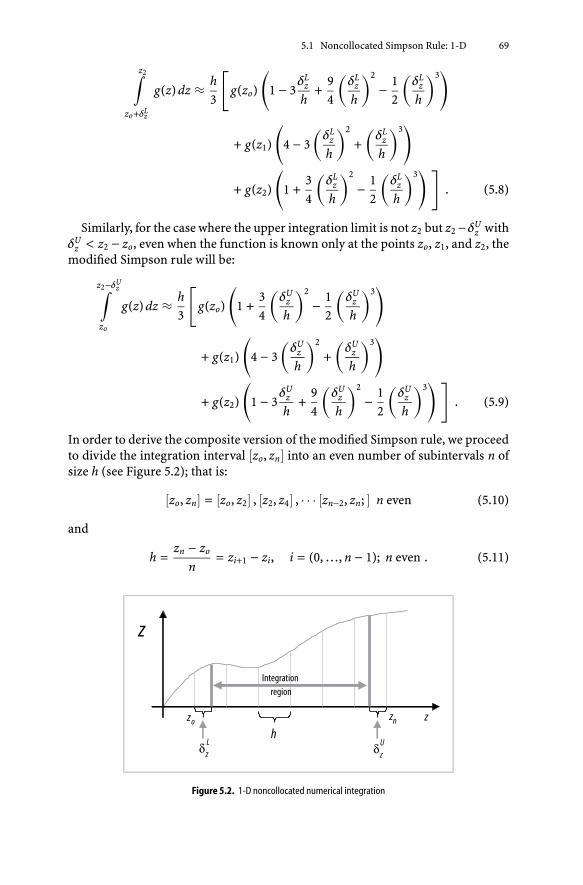
5.1 Noncollocated Simpson Rule: 1-D 69
z2∫
zo+δLz
g(z) dz ≈ h3
[g(zo)
(1 − 3
δLz
h+
94
(δL
z
h
)2
−12
(δL
z
h
)3)
+ g(z1)
(4 − 3
(δL
z
h
)2
+(
δLz
h
)3)
+ g(z2)
(1 +
34
(δL
z
h
)2
−12
(δL
z
h
)3) ]
. (5.8)
Similarly, for the case where the upper integration limit is not z2 but z2 − δUz with
δUz < z2 − zo, even when the function is known only at the points zo, z1, and z2, the
modified Simpson rule will be:
z2−δUz∫
zo
g(z) dz ≈ h3
[g(zo)
(1 +
34
(δU
z
h
)2
−12
(δU
z
h
)3)
+ g(z1)
(4 − 3
(δU
z
h
)2
+(
δUz
h
)3)
+ g(z2)
(1 − 3
δUz
h+
94
(δU
z
h
)2
−12
(δU
z
h
)3) ]
. (5.9)
In order to derive the composite version of the modified Simpson rule, we proceedto divide the integration interval [zo, zn] into an even number of subintervals n ofsize h (see Figure 5.2); that is:
[zo, zn] = [zo, z2] , [z2, z4] , · · · [zn−2, zn; ] n even (5.10)
and
h =zn − zo
n= zi+1 − zi, i = (0, …, n − 1); n even . (5.11)
Figure 5.2. 1-D noncollocated numerical integration

70 5 Two-dimensional Noncollocated Numerical Integration
With this we can write:
zn−δUz∫
zo+δLz
g(z) dz =
z2∫
zo+δLz
g(z) dz +
z4∫
z2
g(z) dz + · · · +
zn−δUz∫
zn−1
g(z) dz . (5.12)
Substituting Equations 5.6, 5.8, and 5.9 into Equation 5.12, we obtain:
zn−δUz∫
zo+δLz
g(z) dz ≈ h3
[g(zo) + 4
n/2−1∑i=0
g(z2i+1) + 2n/2−1∑
i=1
g(z2i) + g(zn)
−⟨V(
δLz
h
), [g(zo) g(z1) g(z2)]T
⟩
−⟨V(
δUz
h
), [g(zn) g(zn−1) g(zn−2)]T
⟩ ], (5.13)
where
V(ν) =[(
3ν −94ν2 +
12ν3) (
3ν2 − ν3)(
−34ν2 +
12ν3)]
(5.14)
and 〈a, b〉 is the vector inner product operator.Equation 5.13 is the 1-D noncollocated form of Simpson’s integration rule. It is
the well-known 1-D Simpson rule, but with the addition of two correction termscorresponding to the low and high integration limits.
5.2 Noncollocated Simpson Rule: 2-D
The derivation of the 2-D modified Simpson rule follows. The integral of the
function f (x, y) in the interval⌊
xo + δLx , xnx − δU
x
⌋ ×⌊
yo + δLy , yny − δU
y
⌋can be
written as:
yny −δUy∫
yo+δLy
xnx −δUx∫
xo+δLx
f (x, y) dx dy =
yny −δUy∫
yo+δLy
g(y) dy , (5.15)

5.2 Noncollocated Simpson Rule: 2-D 71
where
g(y) =
xnx −δUx∫
xo+δLx
f (x, y) dx . (5.16)
Using Equation 5.13, Equation 5.16 can be approximated as:
g(y) ≈ hx
3
⎡⎣ f (xo, y) + 4
nx2 −1∑i=0
f (x2i+1, y) + 2
nx2 −1∑i=1
f (x2i, y) + f (xnx , y)
−⟨V(
δLx
hx
), [f (xo, y) f (x1, y) f (x2, y)]T
⟩
−⟨V(
δUx
hx
), [f (xnx , y) f (xnx−1, y) f (xnx−2, y)]T
⟩ ⎤⎦ , (5.17)
with
hx =xnx − xo
nx= xi+1 − xi, i = (0, …, nx − 1); nx even . (5.18)
Substituting Equation 5.17 into Equation 5.15, we obtain:
yny −δUy∫
yo+δLy
xnx −δUx∫
xo+δLx
f (x, y) dx dy
≈yny −δU
y∫
yo+δLy
hx
3
[f (xo, y) + 4
nx2 −1∑i=0
f (x2i+1, y) + 2
nx2 −1∑i=1
f (x2i, y) + f (xnx , y)
−⟨V(
δLx
hx
), [f (xo, y) f (x1, y) f (x2, y)]T
⟩
−⟨V(
δUx
hx
), [f (xnx , y) f (xnx−1, y) f (xnx−2, y)]T
⟩ ]dy . (5.19)
Repeating the application of the Simpson rule to Equation 5.19:

72 5 Two-dimensional Noncollocated Numerical Integration
yny −δUy∫
yo+δLy
xnx −δUx∫
xo+δLx
f (x, y) dx dy ≈
≈ hy
3×

5.2 Noncollocated Simpson Rule: 2-D 73
−hy
3×
(5.20)
where
hy =yny − yo
ny= yi+1 − yi , i = (0, …, ny − 1); ny even . (5.21)
Simplifying Equation 5.20, we obtain:
yny −δUy∫
yo+δLy
xnx −δUx∫
xo+δLx
f (x, y) dx dy ≈

74 5 Two-dimensional Noncollocated Numerical Integration

5.2 Noncollocated Simpson Rule: 2-D 75
(5.22)
Performing the summation over each sample of f (x, y), Equation 5.22 can beexpressed in a more compact nomenclature:
yf −δUy∫
yo+δLy
xf −δUx∫
xo+δLx
f (x, y) dx dy
=hxhy
9
nx∑i=0
ny∑j=0
(Si,j − Ri,j
(hx, hy, δL
x , δHx , δL
y , δHy
))f (xi, yj) + ε( f ) , (5.23)

76 5 Two-dimensional Noncollocated Numerical Integration
where
where
VxLi is the ith component of the vector V
(δL
xhx
)
VxUi is the ith component of the vector V
(δU
xhx
)
VyLi is the ith component of the vector V
(δL
yhy
)
VyUi is the ith component of the vector V
(δU
yhy
)

5.2 Noncollocated Simpson Rule: 2-D 77
nx + 1︷ ︸︸ ︷
S =
⎡⎢⎢⎢⎢⎢⎢⎢⎢⎢⎢⎢⎢⎢⎢⎢⎣
1 4 2 4 2 · · · 4 2 4 14 16 8 16 8 · · · 16 8 16 42 8 4 8 4 · · · 8 4 8 24 16 8 16 8 · · · 16 8 16 42 8 4 8 4 · · · 8 4 8 2...
......
......
......
......
4 16 8 16 8 · · · 16 8 16 42 8 4 8 4 · · · 8 4 8 24 16 8 16 8 · · · 16 8 16 41 4 2 4 2 · · · 4 2 4 1
⎤⎥⎥⎥⎥⎥⎥⎥⎥⎥⎥⎥⎥⎥⎥⎥⎦
⎫⎪⎪⎪⎪⎪⎪⎪⎪⎪⎪⎪⎪⎪⎪⎬⎪⎪⎪⎪⎪⎪⎪⎪⎪⎪⎪⎪⎪⎪⎭
ny + 1 , (5.25)
and ε( f ) is the integration error due to the numerical approximation process.Equation 5.23 reveals that knowledge of the 2-D function f (x, y) at the knots of
a rectangular evenly spaced grid allows noncollocated numerical integration withan approximation error ε( f ). The error, ε( f ), is evaluated in Appendix C, where itis shown that the integration error depends on the spacing of the high-resolutionsample grid, i.e., hx, hy, and can be made arbitrarily small by choosing these gridparameters appropriately. The way to derive a suitable grid spacing hx, hy froma specified maximum error is also presented in Appendix C.

6 Computational Tools
A computational tool, called EyeBox, was created to model and visualize the ex-tensive image formation process, as well as to evaluate the CRLB and practicalestimators. This tool was developed using MATLAB®. EyeBox provides a frame-work within which the parameters of the physical model of image formation areorganized, enabling the investigation of landmark location uncertainty using theanalytical framework presented in Chapter 3.
A block diagram of the EyeBox tool is shown in Figure 6.1. This diagram alsoshows the high-level structure of the experimental tool EyeExpBox, which will beintroduced in Chapter 7.
The functional architecture of EyeBox is shown in Plate 6 (see Color Section,page 149). The main inputs to the tool are the parameters provided by a con-figuration file and an experiment name. From here, a sequence of componentsimplements the image formation transformations indicated in Equation 2.4, toestimate landmark position, based on the user-selected estimators, and the relatedconfidence intervals. Table 6.1 presents an example of the typical configuration fileused in EyeBox.
In this chapter, complete descriptions of the EyeBox components are presented,including details on the mathematical treatment of the image formation processesand the calculation of the landmark location uncertainty via the confidence inter-vals generated.
6.1 EyeEntity
EyeEntity is the first component in EyeBox. EyeEntity creates a high-resolution nu-merical model of the optical flux function H(x, y) of a circular landmark. H(x, y)is created via the pinhole model associated with geometric optics, using the ge-ometrical parameters listed in the configuration file. These parameters are thelandmark radius and the six parameters describing the landmark pose in cameracoordinates. The sampling density of the high-resolution grid is also provided bythe user in the configuration file; this parameter should be calculated accordingto the 2-D integration error requirements of the spatial sampling presented inChapter 5 and Appendix C.
EyeEntity also creates the illuminance function E(x, y). This is achieved byconvolving the optical flux function H(x, y) with the 2-D impulse response of the

80 6 Computational Tools
Figu
re6.
1.Bl
ock
diag
ram
ofEy
eBox
and
EyeE
xpBo
x

6.1 EyeEntity 81
Table 6.1. Example configuration file for EyeBox. Types are ’s’ string, ’d’ integer, ’f’ floating point, and ’v’ vector of floatingpoint.
Parameter Value Type Description
CameraName PULNiX9701 s Imager mode based on the Pulnix 9701LensName 35mmDG s Double Gauss 35-mm lensFrameGrabberName mv1500 s SimulatedNx 20 d Imager resolution: horizontal [pixels]Ny 20 d Imager resolution: vertical [pixels]Sblur 0.005 f Diffraction blur radius [mm]Std. Deviation Noise 0.004 f Standard deviation of noise in imager: 1/28
wx 80% f Percentage pixel sensitive area on xCamera wy 80% f Percentage pixel sensitive area on y
kx 83 f Pixel density in x. kx = Nx/width[pixel/mm]
ky 73 f Pixel density in y. ky = Ny/height[pixel/mm]
x0 10 f Principal point, x coordinate [pixels]y0 10 f Principal point, y coordinate [pixels]cp 35 f Principal distance [mm]K [0 0] v Radial lens distortion parametersP [0 0] v Decentering lens distortion parametersbZoomLens 0 f No zoomConfigName TestDisk s Small diskArtworkName Disk s Circular landmarkcR_L 3 f Landmark radius [mm]cX_L 0 f x coordinate of landmark center
in camera coordinates [mm]cY_L 0 f y coordinate of landmark center
in camera coordinates [mm]Land- cZ_L 2700 f z coordinate of landmark centermark in camera coordinates [mm]
cPitch_L 0 f Pitch of target in camera coordinatescRoll_L 10 f Roll of target in camera coordinatescYaw_L 0 f Yaw of target in camera coordinatesLmin 0.2 f Luminosity dark [fraction of full scale]Lmax 0.8 f Luminosity light [fraction of full scale]Rect [] v For use in EyeExpBoxKIG 0 f Nonuniform illumination rate
[intensity/mm]AngleIG 0 f Nonuniform illumination plane angle
[degrees]
lens system. The spatial impulse response is approximated by a 2-D Gaussian withvariance σ2
b (see Section 2.1), where σb is the diffraction smoothing parameter fromthe configuration file (see Plate 7 in the Color Section, page 150). The Gaussiankernel used in the smoothing process is sampled with the same spatial grid used inthe creation of H(x, y). A sample screenshot of the EyeEntity component is shownin Figure 6.2.
EyeEntity stores landmark, camera, and other ancillary description information,along with the generated optical flux and illuminance functions, in a MATLAB®
data file for subsequent processing.
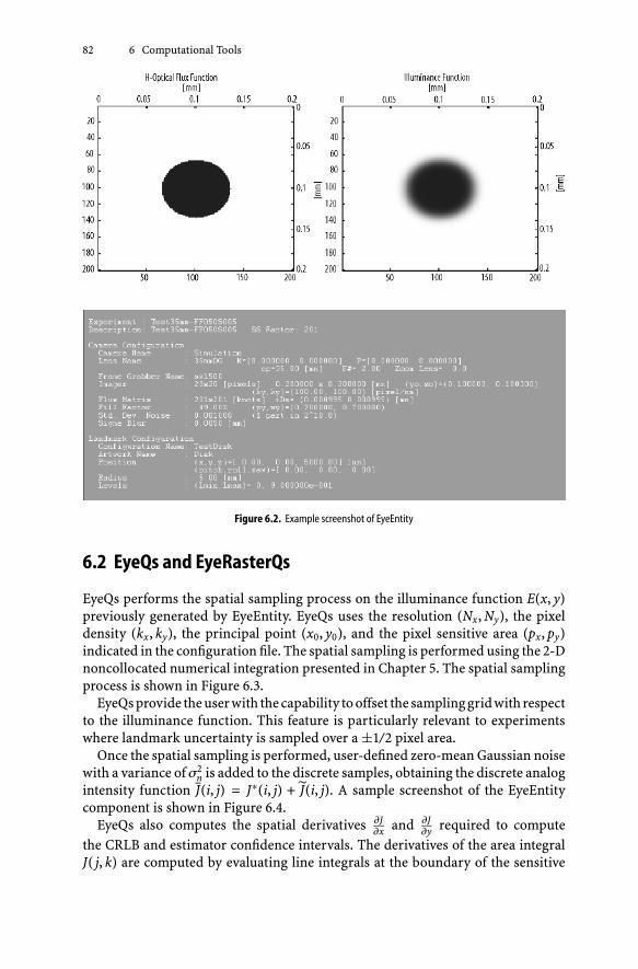
82 6 Computational Tools
Figure 6.2. Example screenshot of EyeEntity
6.2 EyeQs and EyeRasterQs
EyeQs performs the spatial sampling process on the illuminance function E(x, y)previously generated by EyeEntity. EyeQs uses the resolution (Nx, Ny), the pixeldensity (kx, ky), the principal point (x0, y0), and the pixel sensitive area (px, py)indicated in the configuration file. The spatial sampling is performed using the 2-Dnoncollocated numerical integration presented in Chapter 5. The spatial samplingprocess is shown in Figure 6.3.
EyeQs provide the user with the capability to offset the sampling grid with respectto the illuminance function. This feature is particularly relevant to experimentswhere landmark uncertainty is sampled over a ±1/2 pixel area.
Once the spatial sampling is performed, user-defined zero-mean Gaussian noisewith a variance of σ2
n is added to the discrete samples, obtaining the discrete analogintensity function J(i, j) = J∗(i, j) + J(i, j). A sample screenshot of the EyeEntitycomponent is shown in Figure 6.4.
EyeQs also computes the spatial derivatives ∂J∂x and ∂J
∂y required to computethe CRLB and estimator confidence intervals. The derivatives of the area integralJ( j, k) are computed by evaluating line integrals at the boundary of the sensitive

6.2 EyeQs and EyeRasterQs 83
Figure 6.3. Spatial sampling process
Figure 6.4. Example screenshot of EyeQs

84 6 Computational Tools
area corresponding to J( j, k). These line integrations are performed within the 2-Dnoncollocated numerical integration routine. Numerical first difference is not used.
EyeRasterQs is functionally similar to EyeQs, but was created to perform au-tomated raster spatial quantization in the ±1/2 pixel area to model the uniformprobability distribution of the true landmark location in the pixel. The resultsfrom EyeQs and EyeRasterQs are stored for subsequent use of the remaining Eye-Box components.
6.3 EyeQi and EyeRasterQi
The amplitude quantization transformation is performed by EyeQi. Using thiscomponent, the amplitude of the discrete analog intensity function J(i, j) is quan-tized by a uniform quantizer to form the digital image function I(i, j). This processis illustrated in Figure 6.5.
Figure 6.5. Amplitude quantization process
Similarly, EyeRasterQi performs the amplitude quantization task for the discreteanalog intensity functions generated by EyeRasterQs.
EyeQi and EyeRasterQi generate digital image functions for selected quantifica-tion levels in the range of q = [1 … 16], and the results are stored so that they canbe used by the EyeT component described below.
6.4 EyeT
EyeT is the EyeBox component in charge of performing landmark location esti-mation for both discrete analog amplitude functions and digital images. The es-timators used in EyeT are binary centroid, grayscale centroid, ellipsoidal contour,and Butterworth tepuy. In order to accommodate corrections for lens distortionand the geometry of non-square pixels, these estimators are implemented in imagecoordinates; that is [ix, iy]T , in millimeters, rather than in pixel coordinates. Theestimation process is illustrated in Figure 6.6.

6.5 EyeCI 85
Figure 6.6. Estimation process
EyeT automatically detects whether the experiment corresponds to a single orraster image simulation. In the case of raster simulations, EyeT stores the estimationresults in a special folder for further processing by EyeCI.
6.5 EyeCI
The final component in EyeBox is EyeCI. This tool computes the CRLB and esti-mation confidence intervals according to the framework developed in Chapter 3.
Figure 6.7. Example confidence interval display from EyeCI

86 6 Computational Tools
Circular integrals from Equations 3.16 and 3.42 are evaluated using regular 2-D Simpson integration (not the noncollocated version introduced in this work).Furthermore, the overall confidence interval integration over the ±1/2 pixel area,Equations 3.20 and 3.44, was implemented using numerical Euler integration.A sample display of a confidence interval computation performed by EyeCI isshown in Figure 6.7.
The confidence interval shown is the result of processing the configuration calledTest35mm-Baseline3 on digital images quantized at eight bits (q = 8) using theButterworth tepuy estimators (denoted “E” in the figure legend). The noise levelapplied to this experiment was 1/256th of the full scale of the imager considered,modeling σb = 1.0 count for the eight-bit ADC. Figure 6.7 also shows the distribu-tion of the estimator bias; this information is relevant since it provides an indicationof the effect of bias on the uncertainty level. For the configuration investigated toproduce Plate 7, bias contributes a large portion of the total uncertainty.
Confidence intervals for both the CRLB and practical estimators can be com-puted with the EyeBox tool. Chapter 8 presents the results from numerical exper-iments performed using the EyeBox tool in order to study the impact of selectedcharacteristics on precision landmark location.

7 Experimental Validation
This section reports an experiment that was designed to directly measure theuncertainty of landmark location estimates. The experiment is used to test andvalidate the theoretical framework developed in Chapters 2 and 3. The outcomesof these experiments are confidence interval maps for four landmark locationestimators: binary centroid, the grayscale centroid, ellipsoidal contour, and theButterworth tepuy.
Landmark location estimator error is given by:
pPo = pPo − pP∗o , (7.1)
where pP0 is given by the estimator under test. The challenge when directly measur-ing location accuracy is to obtain a suitable value for pP∗
o , the true position of thelandmark. With the three- and seven-pixel-diameter circular landmarks tested,the CRLB shows a minimum uncertainty of about 20 millipixels, so pP∗
o must bedetermined to within one or a few millipixels for the accurate measurement of pPo.This is achieved by surrounding the primary landmark with a secondary landmarkthat is much larger, and thereby presents many more pixels for location estima-tion. Furthermore, the secondary landmark is designed so that some possible biaseffects are cancelled by symmetry, and also so that an internal measure of accuracyis provided by redundancy.
Chapter 7 is organized as follows. Section 7.1 presents the details of the ex-perimental design and setup. Section 7.2 introduces the innovative experimentalmethodology that allows the determination of landmark location pP∗
o with veryhigh accuracy. The camera calibration and focusing procedure is presented inSection 7.3, followed by imager noise characterization in Section 7.4. Finally, theexperimental tool that enables experimental validation is presented in Section 7.5,followed by experimental results in Section 7.6.
7.1 Experiment Design and Setup
Experiments have been performed on an isolated optical bench using a PulnixTM-9701 monochrome digital camera and 18- and 35-mm double Gauss lenses.The camera characteristics are listed in Table 7.1. The data for each experimentcomprised 1800 images, three images at each of 600 positions. The landmark

88 7 Experimental Validation
Figure 7.1. Experimental setup
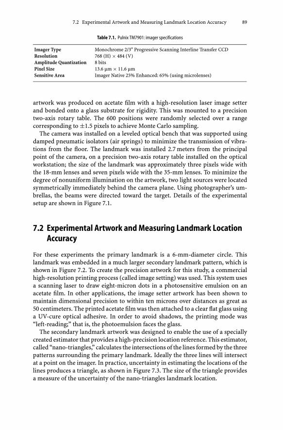
7.2 Experimental Artwork and Measuring Landmark Location Accuracy 89
Table 7.1. Pulnix TM7901: imager specifications
Imager Type Monochrome 2/3" Progressive Scanning Interline Transfer CCDResolution 768 (H) × 484 (V)Amplitude Quantization 8 bitsPixel Size 13.6 μm × 11.6 μmSensitive Area Imager Native 25% Enhanced: 65% (using microlenses)
artwork was produced on acetate film with a high-resolution laser image setterand bonded onto a glass substrate for rigidity. This was mounted to a precisiontwo-axis rotary table. The 600 positions were randomly selected over a rangecorresponding to ±1.5 pixels to achieve Monte Carlo sampling.
The camera was installed on a leveled optical bench that was supported usingdamped pneumatic isolators (air springs) to minimize the transmission of vibra-tions from the floor. The landmark was installed 2.7 meters from the principalpoint of the camera, on a precision two-axis rotary table installed on the opticalworkstation; the size of the landmark was approximately three pixels wide withthe 18-mm lenses and seven pixels wide with the 35-mm lenses. To minimize thedegree of nonuniform illumination on the artwork, two light sources were locatedsymmetrically immediately behind the camera plane. Using photographer’s um-brellas, the beams were directed toward the target. Details of the experimentalsetup are shown in Figure 7.1.
7.2 Experimental Artwork and Measuring Landmark LocationAccuracy
For these experiments the primary landmark is a 6-mm-diameter circle. Thislandmark was embedded in a much larger secondary landmark pattern, which isshown in Figure 7.2. To create the precision artwork for this study, a commercialhigh-resolution printing process (called image setting) was used. This system usesa scanning laser to draw eight-micron dots in a photosensitive emulsion on anacetate film. In other applications, the image setter artwork has been shown tomaintain dimensional precision to within ten microns over distances as great as50 centimeters. The printed acetate film was then attached to a clear flat glass usinga UV-cure optical adhesive. In order to avoid shadows, the printing mode was“left-reading;” that is, the photoemulsion faces the glass.
The secondary landmark artwork was designed to enable the use of a speciallycreated estimator that provides a high-precision location reference. This estimator,called “nano-triangles,” calculates the intersections of the lines formed by the threepatterns surrounding the primary landmark. Ideally the three lines will intersectat a point on the imager. In practice, uncertainty in estimating the locations of thelines produces a triangle, as shown in Figure 7.3. The size of the triangle providesa measure of the uncertainty of the nano-triangles landmark location.

90 7 Experimental Validation
Figure 7.2. Landmark location experiment artwork design
The artwork is composed of three line-location patterns. Each of these patternsis composed of pattern boxes whose central edges are collinear with the patternline used for high-precision location. These definitions are shown in Figure 7.3.
In order to locate the three pattern lines, the central edge in each of the line-location patterns must be found. There are a variety of edge detection algorithms(Heath et al. 1996), but to ensure the lowest estimation uncertainty, a methodologygeneralizing the Nalwa–Binford subpixel edge location algorithm was developed(Nalwa and Binford 1986). The features added to the Nalwa–Binford algorithm are:
• Detection of multiple edges around the same line.
• Use of selected pixels for edge location estimation (the original Nalwa–Binfordalgorithm operates with data from a 5 × 5 pixel image region incorporating theedge).
• New multistage seeding of the nonlinear line location estimator, as describedbelow.
The generalized Nalwa–Binford algorithm models the central edges of the high-precision line location patterns with a hyperbolic tangent of the form:
L(z) = Knb ± Snb tanh(
fnb(z − p))
; z = x sin α + y cos α , (7.2)

7.2 Experimental Artwork and Measuring Landmark Location Accuracy 91
Figure 7.3. Definitions of the artwork features used in the discussion of the “nano-triangles” estimator
where Knb is the mid-level of the edge with units of intensity, Snb is the intensitydifference between the light and dark sides of the line, fnb is a constant determinedby the smoothing of the imaging system (in mm−1), i.e., σb, p is the distance ofthe edge with respect to the origin of the coordinates (in mm) and finally α isthe direction of intensity variation on the edge (in degrees). These definitions areillustrated in Figure 7.4.
Figure 7.4. Hyperbolic tangent model for edges

92 7 Experimental Validation
Figure 7.5. Surface pictorial of a portion of the artwork pattern. Illuminance intensity is indicated by the z coordinate ofthe mesh plot. As with the primary landmark, the illuminance makes a smooth transition from the high to low level.
An alternating box pattern is used in the artwork to compensate for any first-order bias in the edge location estimator. A mesh plot of the artwork image is shownin Figure 7.5, where the height at each point indicates the illuminance function atthe corresponding point in the image. The symmetric alternation of pattern boxesbetween the left and right sides of the line tends to cancel any bias present in theedge location estimate.
The model used for the estimation of each of the three pattern line locations is:
L(z) =5∑
j=1
[Kj
nb + Sjnb tanh
(fnb(z − p)
)]∣∣∣box=2∗j−1
+[
Kjnb − Sj
nb tanh(fnb(z − p)
)]∣∣∣box=2∗j
z = x sin α + y cos α . (7.3)
In this model there are several parameters Kjnb and Sj
nb corresponding to the illu-mination intensity levels in neighboring pattern boxes. These parameters accountfor the effects of nonuniform illumination across the entire length of the patternline. With the model presented in Equation 7.3, a nonlinear least squares estimatorwith 12 parameters, θ = K1
nb, S1nb, K2
nb, S2nb, K3
nb, S3nb, K4
nb, S4nb, K5
nb, S5nb, p, α, is solved
using the Newton–Raphson method.The three pattern lines give three intersection points, as illustrated in Figure 7.6.
The estimated location of the center of the landmark is calculated as the centroid ofthe intersection points. The uncertainty in this estimation is calculated as the normof the vector formed between the estimated center and the farthest intersectionpoint from it. Examples of the output from the nano-triangles estimator for twoexperimental images are shown in Figure 7.6.
The three edges that form the triangles seen in Figure 7.6 are independentlyestimated from the pattern lines of the secondary landmark, and would ideallyintersect at a point. The size of the triangle is an indication of the uncertainty

7.2 Experimental Artwork and Measuring Landmark Location Accuracy 93
Figure 7.6a,b. Example output of the nano-triangles estimator: a 35-mm image; b 18-mm image. The one and threenanometer indications are the typical dimensions of the triangles formed, as measured on the surface of the imager. Onenanometer is approximately 100 micropixels.
in the location of the image of the center of the secondary landmark. As seen inFigure 7.6, the misfit triangles have dimensions of approximately one nanometeron the imager (or approximately 0.1 millipixels) when imaged with the 35-mm lens,and three nanometers when imaged with the 18-mm lens. To highlight the accuracyof the nano-triangles location estimate, Figure 7.6 also shows a picture of the outerelectron orbital of a nitrogen molecule taken recently at the Steacie Institute forMolecular Sciences1. As a separate measure of the secondary landmark locationuncertainty, 30 images were taken with each lens at a single pose, and the secondarylandmark was located in each image. These sets show a one-sigma variability oftwo millipixels for the 35-mm lens configuration and five millipixels for the 18-mmlens configuration. While significantly different from each other, both the triangledimensions and the image-to-image variability support the conclusion that thereference locations given by the nano-triangles estimator are sufficiently accurateto be used to experimentally measure the primary landmark location uncertainty.
1 Nitrogen molecule picture courtesy of Dr. David Villeneuve from the Steacie Institute for MolecularSciences, part of the National Research Council in Canada. Reproduced with permission.
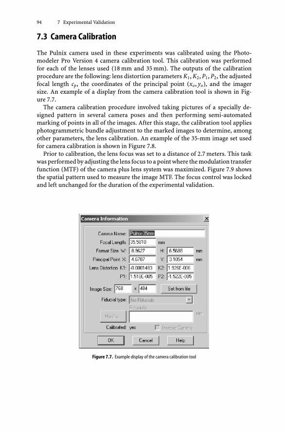
94 7 Experimental Validation
7.3 Camera Calibration
The Pulnix camera used in these experiments was calibrated using the Photo-modeler Pro Version 4 camera calibration tool. This calibration was performedfor each of the lenses used (18 mm and 35 mm). The outputs of the calibrationprocedure are the following: lens distortion parameters K1, K2, P1, P2, the adjustedfocal length cp, the coordinates of the principal point (xo, yo), and the imagersize. An example of a display from the camera calibration tool is shown in Fig-ure 7.7.
The camera calibration procedure involved taking pictures of a specially de-signed pattern in several camera poses and then performing semi-automatedmarking of points in all of the images. After this stage, the calibration tool appliesphotogrammetric bundle adjustment to the marked images to determine, amongother parameters, the lens calibration. An example of the 35-mm image set usedfor camera calibration is shown in Figure 7.8.
Prior to calibration, the lens focus was set to a distance of 2.7 meters. This taskwas performed by adjusting the lens focus to a point where the modulation transferfunction (MTF) of the camera plus lens system was maximized. Figure 7.9 showsthe spatial pattern used to measure the image MTF. The focus control was lockedand left unchanged for the duration of the experimental validation.
Figure 7.7. Example display of the camera calibration tool

7.3 Camera Calibration 95
Figure 7.8. Camera calibration images for 35-mm lens
Figure 7.9. Picture of spatial pattern used for camera focusing

96 7 Experimental Validation
7.4 Imager Noise Characterization
A study of the imager noise behavior of the Pulnix TM9701 is presented in thissection. The characterization is performed by calculating the RMS standard de-viation σJ of the pixel values from a given image captured M times. Assuming animager with a
(Nx, Ny
)pixel resolution, the RMS variance is given by
σ2J =
Nx∑j=1
Ny∑k
M∑i=1
(I( j,k,i) − E
{I( j,k)
})2
NxNy(M − 1
) , (7.4)
where I( j,k,i) is the ith measured intensity of the ( j, k) pixel and E{
I( j,k)}
is theexpected value of the measurements,
E{
I( j,k)}
=
M∑i=1
I( j,k,i)
M. (7.5)
Application of Equation 7.4 to a set of images acquired using the Pulnix TM9701with a 35-mm lens is shown in Figure 7.10. It is important to highlight the fact that
Figure 7.10. Pulnix TM9701 noise characterization: 35-mm lens

7.5 Experimental Tool 97
Figure 7.11. Pulnix TM9701 noise characterization: dark image
the study was performed for the full image, as well as for sections of it, in order toinvestigate the possibility of nonuniform noise behavior in the imager.
This characterization confirms the hypothesis of Gaussian-distributed noise andreveals that σJ is approximately one count of the Pulnix TM9701 eight-bit imager.An equivalent outcome was obtained when the same experiment was performedusing an 18-mm lens.
Figure 7.11 shows the measurement of σJ using dark images (i.e., with a lenscover installed). Notice that the dark current noise level is about 40% lower thanthat of the illuminated images. This indicates a coupling between the noise leveland the illumination intensity captured on the imager, which is expected to havea contribution due to shot noise. For this research, a simplified noise model whichneglects the intensity-dependent component of σJ is used.
7.5 Experimental Tool
A computational tool for automatically computing estimation confidence intervalswas developed in order to realize the experimental validation. This tool, calledEyeExpBox, was built using MATLAB®. EyeExpBox provides a framework for cal-culating landmark location uncertainty in experimental images. To accomplishthis, EyeExpBox processing is divided into a set of computational components im-plemented in MATLAB® program files. The high-level architecture of EyeExpBoxis shown in Plate 8 (see Color Section, page 151).
The first component of EyeExpBox is ProcLA. This photogrammetric tool de-termines the pose of the artwork with respect to the camera, enabling artworkfeatures to be accurately located during further processing. In addition, this toolcreates and stores other data structures related to the experimental configurationand camera information, including camera calibration parameters.
Image files processed by ProcLA are then passed to EyeExpConfig. This toolhas several functions. First, it creates the file structure for each subsequent stepof EyeExpBox. Second, it adds ancillary configuration information such as cameramodel, landmark type, and experimental description, to the data structures createdby ProcLA. Finally, EyeExpConfig computes a high-precision estimate of the center

98 7 Experimental Validation
of the landmark image by performing the nano-triangles estimation, as explainedin Section 7.2. The results of this estimation are then stored for further processingin the subsequent set of EyeExpBox tools.
Figure 7.12 shows the display created by EyeExpConfig while processing one ofthe experimental images. Notice the marking of the corners of the pattern boxes.These points are located using the target-pose estimate provided by ProcLA. Thecircular areas around the boxes’ center edges indicate the pixels that are used bythe nano-triangles estimator.
EyeExpDisk is the tool responsible for separating the image of the landmarkfrom the image of the artwork. This is done by estimating the landmark centerusing the nano-triangles algorithm, and then extracting the set of pixels withina radius from this point. The radius is calculated as the mid-point between theouter edge of the landmark and the closest pattern box. Figure 7.13 shows anexample of the landmark separation process executed by EyeExpDisk.
The next tool within EyeExpBox is EyeExpT. This tool applies landmark locationestimators to the separated images. As in the case of EyeT (see Section 6.4), theestimators used in EyeExpT are binary centroid, grayscale centroid, ellipsoidal con-
Figure 7.12. Display generated by EyeExpBox. Bright circles show pixels selected for processing by the nano-trianglesestimator.
Figure 7.13. Landmark separation performed by EyeExpDisk

7.6 Experimental Results 99
tour, and Butterworth tepuy. In line with photogrammetric practice, the landmarklocation estimators are implemented in image coordinates.
Finally, EyeExpCov processes the estimates from the EyeExpT and generatesexperimental estimation confidence intervals. The confidence interval for a givenestimator is calculated as follows:
• For each estimate from the Monte Carlo sampling, form:
PoL( j, T) = Po
L( j, T) − P∗
oL( j) 1 ≤ j ≤ M , (7.6)
where P∗oL(j) is the jth estimate of the secondary landmark location obtained
from the nano-triangles estimator from the M experimental repetitions, PoL(j, T)
is the estimated center of the landmark image from the jth image, obtained usingestimator T, and Po
L(j, T) is the misadjustment of the estimator.
• The calculated misadjustments are sorted into order of ascending magnitude,∥∥∥PoL
(k − 1, T
)∥∥∥ ≤∥∥∥Po
L
(k, T
)∥∥∥ ≤∥∥∥Po
L
(k + 1, T
)∥∥∥ with 1 < k < M.
• The confidence interval of estimator T is given as:
CnT
=∥∥∥Po
L
(k, T
)∥∥∥ , k = n ∗ M 0 < n ≤ 1 . (7.7)
Example displays from the EyeExpCov tool are presented in the next section.
7.6 Experimental Results
This section describes experimental results for the confidence interval and thecorresponding probability density function of the studied estimators. The studywas conducted using the two configurations indicated in Section 7.1, processing1800 images; 600 poses and three images acquired at each pose.
18-mm Configuration
The confidence interval results from the 18-mm configuration are shown in Plate 9(see Color Section, page 152). These confidence intervals are computed as the ringscentered around the estimated true center of the landmark image that encloses95% of the Monte Carlo samples for each estimator used.
Plate 10 (see Color Section, page 152) displays the same confidence intervalswithout the Monte Carlo sample details, highlighting E
{pPo
}for each of the esti-
mators used.Figure 7.14 shows the experimentally determined distributions of landmark
location error obtained using an 18-mm lens.As expected, the binary centroid estimator presents the greatest uncertainty.
This is followed by the grayscale centroid estimator, which substantially reduces

100 7 Experimental Validation
Figure 7.14. 18-mm configuration: experimentally determined distributions of landmark location error
uncertainty. The 95% confidence level for the binary centroid algorithm is 345 milli-pixels, while it is 169 millipixels for the grayscaled centroid.
The model-based ellipsoidal contour and Butterworth tepuy estimators showmuch lower uncertainties than the centroid estimators. The model-based estima-tors show near-identical performance, with a 95% confidence interval of 63 milli-pixels. The reduction in estimator bias achieved by explicitly modeling the land-mark shape is a chief contributor to the improvement. The Butterworth tepuyalgorithm shows a performance that is few millipixels better than the ellipsoidalcontour estimator, even though the computational cost of the Butterworth tepuyalgorithm is approximately 30 times greater than that of the ellipsoidal contour.
35-mm Configuration
The confidence interval results for the 35-mm configuration are shown in Plate 11(see Color Section, page 153). This plate also displays E
{pPo
}for each of the
estimators used. Figure 7.15 shows the experimentally determined distributionsof landmark location error obtained using the 35-mm lens.
These results reveal a similar behavior to the one obtained for the 18-mmconfiguration experiment. The binary centroid estimator displays a 95% confidencelevel near 300 millipixels, while the grayscale centroid estimator features the sameconfidence level at 260 millipixels.
The ellipsoidal contour and Butterworth tepuy estimators continue to showa much higher performance, with 95% confidence levels of 52 and 50 millipixels,

7.6 Experimental Results 101
Figure 7.15. 35-mm configuration: experimentally determined distributions of landmark location error
respectively. Again, the performance of the Butterworth tepuy estimator is slightlybetter than that of the ellipsoidal contour estimator.
Plates 10 and 11 show the existence of a bias of approximately 0.015 pixels forthe higher-accuracy ellipsoidal contour and Butterworth tepuy estimators (andlarger for the centroid estimators). Several hypotheses were considered to explainthe bias, including an offset in the artwork, nonuniform lighting, and an imager-related artifact. Experiments were designed to test each hypothesis and data werecollected:
• Rotating the artwork by 180° while keeping the rest of the configuration intact
• Rotating the camera by 180° while keeping the rest of the original configurationunchanged
• Modifying the lighting
However, the results obtained were inconclusive. It is believed that the residualbiases are due to a combination of effects.
The nano-triangles artwork and estimation algorithm gives a reference in theimage with an uncertainty of two millipixels in the 35-mm configuration and fivemillipixels in the 18-mm configuration, which is much less than the uncertaintyprimary landmark location estimator in each case. This experiment provides themeans to directly measure the uncertainty of the primary landmark locationestimators. Measurements show that the model-based estimators perform withsignificantly lower uncertainty than the centroid estimators, providing a five- tosixfold improvement.

8 Studies of Landmark Location Uncertainty
The EyeBox tool provides the means to examine the potential and actual land-mark location uncertainty as a function of landmark and imager configuration. Inthis chapter, the tool is employed to investigate the interactions of imager noise,smoothing radius, luminosity dynamic range, landmark size and tilt, imager pixelsensitive area and aspect ratio, nonuniform illumination and imager amplitudequantization on landmark location uncertainty. These results are presented in theform of performance maps showing the size of the 95% uncertainty confidence
Table 8.1. Baseline configuration for the experimental and numerical investigations
Parameter Value Description
Camera Camera Name PULNiX9701 Imager mode based on the Pulnix 9701Lens 18mm/35mmDG Double Gauss lensAmplitude 8 bits Quantization level over dynamic rangeQuantizationNx 768 Imager resolution: horizontal [pixels]Ny 484 Imager resolution: vertical [pixels]Sblur 0.009 Diffraction blur radius [mm]Std. 0.004 Standard deviation of noise in imager: 1/28
Deviation Noisewx 80% Percentage pixel sensitive area on x axiswy 80% Percentage pixel sensitive area on y axiskx 83 Pixel density in x. kx = Nx/width [pixel/mm]ky 73 Pixel density in y. ky = Ny/height [pixel/mm]cp 18/35 Principal distance [mm]
Landmark cR_L 3 Landmark radius [mm]cX_L 0 x coordinate of landmark center
in camera coordinates [mm]cY_L 0 y coordinate of landmark center
in camera coordinates [mm]cZ_L 2700 z coordinate of landmark center
in camera coordinates [mm]cPitch_L variable Pitch of target in camera coordinatescRoll_L variable Roll of target in camera coordinatescYaw_L variable Yaw of target in camera coordinatesLmin 0.6 Luminosity dark [fraction of full scale]Lmax 0.9 Luminosity light [fraction of full scale]

104 8 Studies of Landmark Location Uncertainty
interval, following the framework developed in Chapter 3. In each case, the experi-mental configuration described in Chapter 7 is taken as the baseline configuration,the parameters of which are listed in Table 8.1. In Section 8.1, analytic calculationsof landmark location uncertainty are validated against the experimental measure-ments. In Sections 8.2 through 8.9, the analytic tools are used to investigate theimpact on uncertainty of a range of configuration variables.
8.1 Theoretical and Experimental Determinationof Landmark Location Uncertainty
Figure 8.1 shows the 95% confidence interval performance maps of the four estima-tors: the binary and grayscale centroid estimators and the ellipsoidal contour andButterworth tepuy estimators. The performance maps include the Cramér–Raolower bound, determined as described in Section 3.1; analytic results for each esti-mator, determined as described in Section 3.2; and experimental results obtainedas described in Chapter 7. The data of Figure 8.1 are shown in Table 8.2.
To generate analytic results, the EyeBox configuration file was set with parame-ters that mimicked the experimental setup. Camera parameters were obtained fromthe camera calibration procedure, artwork location was obtained by the use of thenano-triangles algorithm, and landmark specification was taken from the file used
Figure 8.1. Performances of landmark location estimators; experimental and analytical determinations

8.1 Theoretical and Experimental Determination of Landmark Location Uncertainty 105
Table 8.2. Radius of 95% circular confidence interval for the experimental configuration, showing values given by theanalysis method of Section 3.2, the experiments of Chapter 7, and the Cramér–Rao lower bound calculation of Section 3.1;for the experimental configurations with the 35-mm and 18-mm lenses.
Method 35-mm lens 18-mm lens
Binary centroidAnalysis 212.5 276.5Experiment 296.0 345.0
Grayscale centroidAnalysis 185.5 257.0Experiment 261.0 169.0
Ellipsoidal contourAnalysis 21.0 54.0Experiment 51.0 63.0
Butterworth tepuyAnalysis 20.0 40.5Experiment 50.0 62.0
Cramér–Rao lower bound Analysis 17.5 26.0
for the artwork generation. In addition, diffraction smoothing and illuminationlevels were measured using the images generated in the laboratory experimentsusing the Butterworth tepuy algorithm. Finally the nonuniform illumination wasmeasured with a specially designed tool.
Figure 8.2 shows the potential and experimentally achieved circular landmarklocation estimation performance for a 6-mm circle imaged at 2.7 meters using35- and 18-mm lenses in the configuration described above. At the lowest level ofuncertainty is the Cramér–Rao lower bound, with an uncertainty of 20 millipixels.An idealized estimator with Cramér–Rao bound performance would give an es-timate within this distance of the true image of the landmark center in 95% oftrials. Analysis predicts performance levels for the model-based elliptical contourand Butterworth tepuy estimators that are indistinguishable from each other, and
Figure 8.2a,b. Example landmark images from the experimental investigation given the results of Figure 8.1. This studyfocused on landmarks 4–10 pixels across. The expected precision with larger landmarks is investigated in Section 8.5.a Typical landmark image with 35 mm lens; b typical landmark image with 18-mm lens.

106 8 Studies of Landmark Location Uncertainty
slightly higher than the Cramér–Rao lower bound. One of the surprises of thisresearch is that practical estimators can so closely approach the CRLB.
The experimental estimators show a 95% confidence interval of 50 millipixels forthe 35-mm lens (seven-pixel-diameter landmark) and 62 millipixels for the 18-mmlens (four-pixel-diameter landmark). These levels are 2.5× and 3× the analyticpredictions, respectively, indicating that experimental uncertainties exist whichhave not yet been captured in the model. Nonetheless, the agreement betweenthe analytic results and the experiment is striking. With the exception of theexperimental result for the grayscale centroid estimator with the 18-mm lens,the experimental data follow the pattern of the analytic results in detail, witha consistently elevated level of uncertainty in the experimental result relative toanalysis. Figures 8.3 and 8.4 show the joint probability distributions for each of theestimators studied for the 18-mm and 35-mm configurations. These distributionsgive rise to the performance maps corresponding to the analytical results shown inFigure 8.1. These distributions are the result of integration of the landmark locationconfidence intervals, as described in Section 3.2, and show the same structure asthe experimentally generated distributions, seen in Figures 7.14 and 7.15 for the18-mm and 35-mm lenses, respectively.
In Figures 8.3 and 8.4, it is observed that the binary and grayscale centroiddistributions are not smooth. This is due to the bias characteristics of these esti-mators and the nonstationary statistics of landmark location estimation. Runningthe EyeBox tool with a more dense raster resolution would smooth these curves,but at the expense of very long computational time.
The agreement between experiment and analysis seen in Figure 8.1 and theagreement of the distributions in Figures 7.14, 7.15, 8.3, and 8.4 indicates thatthe analysis tools reliably capture the interactions of configuration parametersand landmark location performance. With the analytic tools validated by theagreement of the analytic results with the experimental results, it is now possibleto use the EyeBox tool to investigate interactions between selected configurationparameters and landmark location uncertainty. Sections 8.2 through 8.9 presentanalysis-based studies of these interactions. Results from studies of the 35-mmconfiguration are reported. In each case similar results were obtained for the18-mm configuration.

8.1 Theoretical and Experimental Determination of Landmark Location Uncertainty 107
Figure 8.3a–e. 18-mm configuration: analytically determined radial probability distributions: a binary centroid estimator;b grayscale centroid estimator; c ellipsoidal contour estimator; d Butterworth tepuy estimator; e Cramér–Rao calculation.
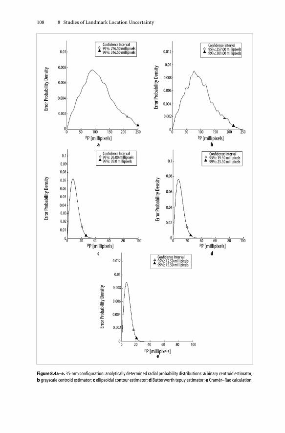
108 8 Studies of Landmark Location Uncertainty
Figure 8.4a–e. 35-mm configuration: analytically determined radial probability distributions: a binary centroid estimator;b grayscale centroid estimator; c ellipsoidal contour estimator; d Butterworth tepuy estimator; e Cramér–Rao calculation.

8.2 Study of Effects of Imager Noise 109
8.2 Study of Effects of Imager Noise
Figure 8.5 presents the results obtained when the imager noise level was increasedfor the 35-mm experimental configuration. Analysis was performed for noise levelsσJ = {1, 2, 4} × (1/256) of full scale. The data for Figure 8.5 are shown in Table 8.3.
As expected, this study shows that the Cramér–Rao lower bound on uncertaintyrises with as imager noise increases. The degree to which the performance of themodel-based estimators tracks the Cramér–Rao lower bound is striking when itis recalled that the CRLB and practical estimator performances are obtained fromvery different calculations. Also striking is the degree to which the binary andgrayscale centroid estimators are insensitive to noise. It is conjectured that thiseffect arises with the averaging that takes place in the calculation of the centroid,and the greater initial uncertainty of these estimators.
Figure 8.5. Landmark location uncertainty performance map: effects of increasing σJ
Table 8.3. Radius of 95% circular confidence interval for three levels of imager noise, determined by analysis for fourestimators and also the Cramér–Rao lower bound. Noise given in units of 1/256 full-scale, or counts of noise for an eight-bitADC. The baseline value for the experimental configuration is 1.0 counts.
MethodNoise level (1/256 full-scale)
1.0 2.0 4.0
Binary centroid 246.0 246.0 247.5Grayscale centroid 219.5 219.0 219.5Ellipsoidal contour 24.0 41.5 79.5Butterworth tepuy 22.0 36.5 68.0Cramér–Rao lower bound 17.5 34.5 68.5

110 8 Studies of Landmark Location Uncertainty
8.3 Study of the Effects of Smoothing Radiuson Landmark Location Uncertainty
Figure 8.6 presents the results obtained when the diffraction-smoothing radius waschanged for the 35-mm experimental configuration. Analysis was performed forsmoothing radii of σb = {1, 4.5, 9, 18} microns. The data for Figure 8.6 are shownin Table 8.4.
Study 8.3 shows that the smoothing introduced by diffraction lowers landmarklocation uncertainty (improves precision) when the smoothing radius is smallerthan a pixel. The pixel dimension of the Pulnix TM9701 camera used for this studyis 13.6 × 11.6 μm. Considering the relation to pixel size, diffraction (or defocus)smoothing up to half the pixel dimension is seen to give a large improvementin precision for the model-based estimators, while smoothing up to the pixeldimension is seen to give a modest improvement for the centroid estimators.
Figure 8.6. Landmark location uncertainty performance map: effects of changing σb
Table 8.4. Radius of 95% circular confidence interval for four values of the smoothing radius σb , determined by analysisfor four estimators and also the Cramér–Rao lower bound. The smoothing operator radius is expressed in microns on theimager surface. The baseline value for the experimental configuration is 9.0 microns.
MethodSmoothing radius (microns)
1.0 4.5 9.0 18.0
Binary centroid 291.5 270.0 246.0 295.0Grayscale centroid 261.5 240.5 219.0 265.0Ellipsoidal contour 50.0 23.5 24.0 41.5Butterworth tepuy 76.0 16.0 22.0 41.5Cramér–Rao lower bound 10.0 13.0 17.5 21.0

8.4 Study of the Effects of Luminosity Dynamic Range 111
8.4 Study of the Effects of Luminosity Dynamic Range
Figure 8.7 presents the results obtained when the luminosity dynamic range wasincreased for the 35-mm experimental configuration. The luminosity dynamicrange is the difference between the background and the landmark luminosity,expressed as a percentage of full scale for the imager. As with the other cases, theanalysis models an eight-bit imager. Analysis was performed for dynamic rangevalues of 30%, 60%, and 80%. The data for Figure 8.7 are shown in Table 8.5.
Study 8.4 shows strongly decreasing uncertainty with increasing dynamic range.While it is expected that increasing the dynamic range will reduce uncertainty, themagnitude of this effect is surprising.
Figure 8.7. Landmark location uncertainty performance map: effects of increasing luminosity dynamic range
Table 8.5. Radius of 95% circular confidence interval, determined by analysis for four estimators and the Cramér–Raolower bound. The luminosity dynamic range is given as the ratio of the landmark interior and exterior luminosity as percentof full scale. The baseline value for the experimental configuration is 30%.
MethodLuminosity dynamic range
30% 60% 80%
Binary centroid 246.0 183.5 144.0Grayscale centroid 219.0 162.5 82.0Ellipsoidal contour 24.0 13.5 11.5Butterworth tepuy 22.0 13.0 11.5Cramér–Rao lower bound 17.5 9.0 6.5

112 8 Studies of Landmark Location Uncertainty
8.5 Study of the Effects of Landmark Size
Figure 8.8 presents the performance maps for different landmark sizes for the35-mm experimental configuration. Analysis was performed for landmark radii of{1.5, 3.0, 6.0, 12.0} millimeters. The baseline configuration (2.7 meters to target,35-mm lens, 11.6 × 13.6 micron pixels) gives 1.1 mm/pixel in the horizontaldirection, so the figures of {1.5, 3.0, 6.0, 12.0} are also approximately the radii ofthe landmarks in pixels. The data for Figure 8.8 are shown in Table 8.6.
It is observed in Study 8.5 that increasing landmark size decreases locationuncertainty for all estimators. Surprisingly, the effect seems to taper off for thecentroid estimators, which reach a minimum level of uncertainty near 150 milli-pixels. For the landmark with a radius of 12 millimeters (a radius of approximately12 pixels in the image), the model-based estimators achieve an expected uncer-tainty of 10 millipixels.
Figure 8.8. Landmark location uncertainty performance map: effects of landmark size
Table 8.6. Radius of 95% circular confidence interval for four values of landmark radius, determined by analysis for fourestimators and also for the Cramér–Rao lower bound. The landmark radius is expressed in units of pixels in the image(root-mean-square radius, to consider perspective distortion or nonsquare pixels). The baseline value for the experimentalconfiguration is 3.0 pixels.
MethodLandmark radius (RMS pixels)
1.5 3.0 6.0 12.0
Binary centroid 344.0 246.0 175.0 161.0Grayscale centroid 324.5 219.0 147.5 125.0Ellipsoidal contour 39.0 24.0 16.0 11.5Butterworth tepuy 35.5 22.0 14.0 9.5Cramér–Rao lower bound 26.0 17.5 12.0 8.5

8.6 Study of the Effects of Landmark Tilt 113
8.6 Study of the Effects of Landmark Tilt
Figure 8.9 presents the results obtained when the pitch was increased for the 35-mmexperimental configuration. The analysis was performed for pitch angles of 0◦, 10◦,20◦, and 30◦.
Out-of-plane rotation, or tilt, is generally avoided in machine vision applications,but it may be unavoidable in photogrammetric or other applications that arecharacterized by a reduced degree of control over the presentation of the landmarkfor imaging. The results from Study 8.6 show that the model-based estimators arerobust to landmark tilt. These estimators each include ellipsoidal eccentricity asa parameter.
Figure 8.9. Landmark location uncertainty performance map: effects of increasing the pitch angle
Table 8.7. Radius of 95% circular confidence interval for four levels of out-of-plane rotation (tilt), determined by analysisfor four estimators and the Cramér–Rao lower bound. Tilt given in degrees. The baseline value for the experimentalconfiguration is 0 degrees.
MethodTilt (degrees)
0 10 20 30
Binary centroid 246.0 209.5 180.0 286.5Grayscale centroid 219.0 223.5 160.0 257.5Ellipsoidal contour 24.0 23.5 24.5 26.5Butterworth tepuy 22.0 23.0 23.0 23.0Cramér–Rao lower bound 17.5 17.5 17.5 18.5

114 8 Studies of Landmark Location Uncertainty
8.7 Study of the Effects of the Pixel Sensitive Areaand Aspect Ratio
Figure 8.10 presents the results obtained when the pixel sensitive area was changedfor the 35-mm experimental configuration, and Figure 8.11 presents the resultsobtained when the pixel sensitive area was changed for the same configuration, withthe smoothing radius changed to 2.0 microns. Figure 8.12 presents the performanceresults for different pixel aspect ratios in the 35-mm experimental configuration.The data for Figures 8.10–8.12 are shown in Tables 8.8–8.10, respectively.
Figure 8.10. Landmark location uncertainty performance map: effects of changing the pixel sensitive area, σb =9.0 microns
Table 8.8. Radius of 95% circular confidence interval for four levels of sensitive area with σb = 9.0 microns, determinedby analysis for four estimators and also the Cramér–Rao lower bound. Sensitive area given as percent of pixel area. Thebaseline value for the experimental configuration is 65%.
MethodSensitive area (percent)
0% 25% 65% 100%
Binary centroid 260.0 254.5 246.0 245.0Grayscale centroid 230.5 225.5 219.0 219.0Ellipsoidal contour 23.0 23.5 24.0 24.0Butterworth tepuy 23.0 23.0 22.0 21.0Cramér–Rao lower bound 15.0 17.0 17.5 18.0

8.7 Study of the Effects of Pixel Sensitive Area and Aspect Ratio 115
Study 8.7 shows the effects of pixel sensitive area and pixel geometry on landmarklocation uncertainty. Figure 8.10 shows that when the smoothing radius (blur) isapproximately the dimension of a pixel, then the pixel sensitive area has a limitedimpact on location uncertainty.
Figure 8.11, in contrast, shows that when the smoothing radius is small relative toa pixel, then sensitive area has a significant impact on the model-based estimators,particularly the ellipsoidal contour algorithm. Over the range investigated, thepixel aspect ratio had minimal effect.
Figure 8.11. Landmark location uncertainty performance map: effects of changing the pixel sensitive area, σb =2.0 microns
Table 8.9. Radius of 95% circular confidence interval for four levels of sensitive area with σb = 2.0 microns, determinedby analysis for four estimators and also the Cramér–Rao lower bound. Sensitive area given as percent of pixel area. Thebaseline value for the experimental configuration is 65%.
MethodSensitive area (percent)
0% 25% 65% 100%
Binary centroid 287.0 287.5 291.5 293.0Grayscale centroid 263.5 260.5 261.0 260.5Ellipsoidal contour 86.5 63.0 42.0 29.5Butterworth tepuy 25.0 20.5 15.5 16.5Cramér–Rao lower bound 7.0 9.5 10.5 11.5

116 8 Studies of Landmark Location Uncertainty
Figure 8.12. Landmark location uncertainty performance map: effects of different pixel aspect ratios
Table 8.10. Radius of 95% circular confidence interval for three values of the pixel aspect ratio, determined by analysisfor four estimators and the Cramér–Rao lower bound. The pixel aspect ratio is the ratio of the smallest to the largest pixeldimensions. The baseline value for the experimental configuration is 1 : 1.17.
MethodPixel aspect ratio
1 : 1 1 : 1.7 1 : 2
Binary centroid 246.5 246.0 251.0Grayscale centroid 219.0 219.0 223.0Ellipsoidal contour 23.5 24.0 23.5Butterworth tepuy 22.5 22.0 23.5Cramér–Rao lower bound 13.0 17.5 17.5
8.8 Study of the Effects of Nonuniform Illuminationon Landmark Location Uncertainty
Figure 8.13 presents the results for the impact of nonuniform illumination onthe 35-mm experimental configuration. In this case, a luminosity gradient wassuperimposed onto the simulated data. The data for Figure 8.13 are presented inTable 8.11.
In this study, the luminosity gradient is expressed as percent variation acrossthe diameter of the landmark. The baseline illuminance is 30% of full scale for theimager, or 77 ADC counts of the eight-bit quantizer. The variations correspond todifferences of zero, three, and six ADC counts of illuminance across the image of thelandmark. Study 8.8 shows that the principal impact of nonuniform illumination isto introduce bias into the model-based estimators, which do not model variation inillumination. The data show that the centroid estimators are robust to nonuniform

8.9 Study of the Effects of Amplitude Quantization 117
Figure 8.13. Landmark location uncertainty performance map: effects of nonuniform illumination
Table 8.11. Radius of 95% circular confidence interval for three values of nonuniform illumination, determined by analysisfor four estimators and the Cramér–Rao lower bound. Nonuniform illumination is expressed in percent variation of luminanceacross the landmark. The baseline value for the experimental configuration is 0 nonuniform illumination.
MethodNonuniform illumination
0.0 4.0% 8.0%
Binary centroid 246.5 252.5 246.5Grayscale centroid 219.0 219.0 222.0Ellipsoidal contour 24.0 27.5 34.0Butterworth tepuy 22.0 28.5 37.0Cramér–Rao lower bound 17.5 17.5 17.5
illumination. The Cramér–Rao lower bound depends on the sensitivity of the datato the displacement of the landmark, and is only affected by bias to the extent thatthe signal grows strong as the illumination is increased toward 100% of full scale.In spite of the marked difference between the models underlying the ellipsoidalcontour and Butterworth tepuy estimators, they are very similarly impacted bynonuniform illumination. This study indicates that the performance of the model-based estimators can be improved by incorporating a representation of nonuniformillumination, for example as a two-element gradient vector.
8.9 Study of the Effects of Amplitude Quantization
Figure 8.14 presents the results for the impact of the amplitude quantizer reso-lution on the 35-mm experimental configuration. Quantizer resolution levels of

118 8 Studies of Landmark Location Uncertainty
Figure 8.14. Landmark location uncertainty performance map: effects of amplitude quantization
Table 8.12. Radius of 95% circular confidence interval for four levels of amplitude quantization, determined by analysisfor four estimators and also the Cramér–Rao lower bound. Quantization is expressed in ADC bits. The baseline value for theexperimental configuration is q = 8 bits.
MethodAmplitude quantization
2 4 8 16
Binary centroid 199.0 198.5 246.5 246.5Grayscale centroid 192.0 174.5 219.0 218.5Ellipsoidal contour 172.0 117.5 24.0 19.0Butterworth tepuy – 102.0 22.0 18.0Cramér–Rao lower bound 17.5 17.5 17.5 17.5
q = {2, 4, 8, 16} bits are considered. A quantizer resolution of one bit is not consid-ered because the grayscale centroid estimator is equivalent to the binary centroidestimator and the model-based estimators are ineffective.
As seen in Figure 2.14, locales grow large when the quantization resolution iscoarse. This is why all estimators approach the same uncertainty for q = 2. TheCramér–Rao bound is calculated for analog intensity data, which do not includeamplitude quantization, and so the CRLB uncertainty is the same in each of thefour cases shown.
For the model-based estimators, the uncertainty drops dramatically with anincrease from four to eight bits of signal. Since the estimators with eight-bitquantization approach the Cramér–Rao lower bound, only a slight improvementin model-based estimator performance is achieved by increasing the quantizerresolution to 16 bits. Recall that the baseline case has an imager noise of 1/256 full

8.9 Study of the Effects of Amplitude Quantization 119
scale, or one count of eight-bit quantization. A lower noise level is expected to leadto an improvement.
At low resolution, most of the uncertainty is due to the locale phenomenon. Forthe baseline configuration considered in this study, the locale phenomenon is lessimportant at a quantization level of eight bits, and the imager noise becomes themain uncertainty factor.

9 Conclusions
The accuracy of image-based measurement depends on the accuracy with whichthe locations of landmarks are determined. This work has advanced the state-of-the-art in precision landmark location in the following ways:
• The confidence interval has been introduced as a measure of landmark locationuncertainty because it is able to accommodate the nonstationary statistics of theproblem
• An extended model of the physics of image formation has been developed, whichcaptures aspects of the physical process that contribute to the determination oflandmark location uncertainty
• The Cramér–Rao lower bound for landmark location uncertainty has been deter-mined, establishing a minimum level of uncertainty for any unbiased estimator,independent of the estimation algorithm used
• A set of tools for analyzing the uncertainties of practical landmark and imagingconfigurations and location estimation algorithms have been created
• Two new, model-based landmark location estimators have been demonstrated,which perform near the Cramér–Rao theoretical limit
• These tools have been validated by developing and performing an experimentthat can directly and accurately measure the error in landmark location esti-mates.
There are many ways to process an image and estimate the location of a landmark.The Cramér–Rao lower bound has been applied to establish the minimum uncer-tainty that any estimator can achieve, given the data and noise present in an image.To carry out the CRLB calculation, it has been necessary to augment the modelof image formation with information about the sensitive area of each pixel anda model that smoothes as an image is formed. When locations are estimated withuncertainties of a small fraction of a pixel, these characteristics play a significantrole. Additionally, smoothing eliminates discontinuities in the illuminance of theimager, rendering the analysis mathematically tractable.
The EyeBox tool kit developed for this study provides a set of tools for ana-lyzing specific landmark, imaging, and estimator configurations. The tool kit hasfunctions for computing the CRLB or analyzing the performances of practicallandmark location estimators. One challenge when studying precision landmark

122 9 Conclusions
location, which is reflected in the EyeBox tool kit, is that precision depends onmany details of configuration. At the limit, where uncertainty is measured in tensof millipixels, the location uncertainty may change by a factor of two when a lensaperture is changed from #f /3 to#f /6. The strength of the tool kit is that it cananalyze a specific imager/landmark configuration, while the weakness is that itmust analyze a specific configuration. Nonetheless, by studying the performanceof specific configurations, systems can be engineered to achieve their maximumperformance.
Inspired by the accuracy of the model-based Nalwa–Binford algorithm for lo-cating edges, two model-based landmark location estimation algorithms havebeen developed. Somewhat to our surprise, these estimators give performancesapproaching the Cramér–Rao lower bound. The ellipsoidal contour algorithm, inparticular, only requires that edge pixels of the landmark image are processed, andhas proven to be a precise and computationally efficient tool.
To validate the EyeBox tool, as well as the Cramér–Rao lower bound, an exper-iment has been performed to directly measure landmark location precision. It isstraightforward to estimate the location of the image of a landmark. It is morechallenging to measure the estimator error, since the latter requires knowledge ofwhere the landmark truly lies. To meet this challenge, a high-precision artworkand an algorithm have been designed that are sufficiently accurate to be used asa reference. The tool, called the nano-triangles estimator, averages over hundredsof pixels, imaging artwork that is laid out in order to cancel first-order error sourcesand to provide a consistency check on its own performance. The nano-trianglesexperiment confirmed the analytic predictions, although at a somewhat higherlevel of uncertainty, indicating that there is an as-yet unmodeled error source inthe landmark location process.
The results of this work answer several questions posed by investigators during30 years of research into landmark location in digital images. As the use of im-ages for measurement grows, the methods and results presented here will providea foundation for the study of diverse imaging, landmark, and estimator configu-rations, new and more complete models of the image formation process, and theengineering of systems to achieve ultimate performance.

Appendix AList of Symbols
Symbol Quantity
* 2-D convolution operatorcp adjusted focal lengthE(ix, iy) illuminance function; parameters in image coordinatesf (Lx, Ly) landmark luminosity function; parameters in landmark coordinates
Gf
(cPo
L
)landmark description transformation
H(ix, iy) optical flux function; parameters in image coordinatesI(i, j) digital image function; parameters in pixel coordinatesJ Fisher information matrixJ1 Bessel function of the first kind and order 1J(i, j) discrete analog intensity function; parameters in pixel coordinatesKo radial lens distortion coefficient: linear termK1 radial lens distortion coefficient: cubic termk propagation numberkx density of pixels in the imager: x direction (in pixels/mm)ky density of pixels in the imager: y direction (in pixels/mm)P1 decentering lens distortion coefficient: x directionP2 decentering lens distortion coefficient: y directionwP point in world coordinates ∈ �3
cP point in camera coordinates ∈ �3
LP point in landmark coordinates ∈ �2
iP point in image coordinates ∈ �2
pP point in pixel coordinates ∈ �2
Qi amplitude quantization transformationQs spatial sampling transformationra Airy disk radiusT(I) estimator of the center of the landmarkΦ geometric optics transfer functionΞ diffraction transfer functionλ wavelengthσb standard deviation of the Gaussian smoothing functionω pitchκ rollϕ yaw

Appendix BGlossary
Aberration: The failure of an optical lens to produce an exact point-to-pointcorrespondence between the object and its resulting image.
ADC: Analog-to-digital converter, used to convert the charge collected in a pixelof an imager to a digital value.
Adjusted focal length: Distance along the principal ray from imager to the principalpoint of the lens, also called the principal distance, cp.
Airy pattern: Diffraction pattern caused by a circular aperture.
Bundle adjustment: an estimation process used in photogrammetry to simultane-ously estimate the locations of target points (landmarks) and the pose of one orseveral camera stations.
Centroid algorithm: A landmark location estimator that operates forming themathematical centroid of the image region identified as the landmark (see Equa-tion (2.22)).
CRLB: Cramér–Rao lower bound; the lower bound on uncertainty of an unbiasedestimate based on the sensitivity of the data to changes in the estimated quantity,and not the noise present in the data.
Cubature formula: Formula used for the numerical computation of a multipleintegral. The 2-D Simpson’s rule is an example of a cubature formula.
DOF: Degrees of freedom, for example an unconstrained body has six degrees ofmotion freedom, or 6 DOF.
Diffraction: Dispersion of light that occurs when light waves pass through a barrier,such as the aperture of a camera. Diffraction has the effect of applying a spatiallow-pass filter to the optical signal.
Digital image function: Function describing the discrete analog intensity functionafter amplitude quantization.
Discrete analog intensity function: Function describing the illuminance functionafter spatial quantization.
Fiducial marks: reference points in a scene that can be used to locate objects orcalibrate measurements.
126 Appendix B
Fill factor: The percentage of photosensitive area within a pixel boundary.
Focal point: A point from which a portion of spherical waves converges or diverges.
Gray level: A quantized measurement of the discrete analog intensity function,typically in the range between pure white and black.
Grayscale: Variations in values from white through shades of gray to black ina digitized image, where black is assigned a value of zero and white a value of one.
Grayscale image: An image consisting of an array of pixels whose intensities cantake more than two values.
Illuminance: The intensity of the light incident on a surface (in lux). Digital imagersensitivity is often specified in counts/lux-second. (See also luminance).
Illuminance function: function representing the distribution of optical flux on theimager, including consideration of diffraction.
Image capture: The process of acquiring an image of a scene, from sensor irradia-tion to acquisition of a digital image.
Image distortion: A situation in which the image is not exactly true to scale to theobject scale.
Image formation: Generation of an image of an object or scene on the imagingsensor. It includes effects from the optics, illumination and the imager itself.
Image plane: The plane surface of the imaging sensor perpendicular to the principalray.
Image processing: Digital manipulation of an image to aid feature visibility, makemeasurements or to alter image contents.
Landmark description transformation: Transformation that creates the landmarkluminosity function from the pose of its center.
Landmark luminosity function: Function that describes the landmark geometryon the landmark plane.
Locale: Equivalence class of the landmark location.
Luminance: The measure of intensity of light radiated from a surface in a particulardirection, [candela/meter2]. (See also illuminance).
Machine vision: The use of devices for optical noncontact sensing to automaticallyreceive and interpret an image of a real scene, in order to obtain information and/orcontrol machines or processes.
MTF: Modulation transfer function, a description of the ability of an optical systemto transfer contrast at a given spatial frequency (e.g., cycles per millimeter ona target at a standard distance). Lens systems generally form low-pass filters, andso higher spatial frequencies are attenuated.
Optical flux function: Function representing the spatial distribution of the land-mark’s luminosity after transformation via geometrical optics, but without con-

Appendix B 127
sidering diffraction smoothing. Examples that contrast the optical flux functionand illuminance function can be seen in Figures 2.1 and 2.3.
Photogrammetry: Science and art of taking measurements from images.
Pixel: An area element of an image. In a monochrome digital image, each pixelcorresponds to a number that is the intensity (illuminance) on the pixel’s sensitivearea.
Principal distance: See adjusted focal length.
Principal point, image: Point where the principal ray intersects the image plane,the origin of image coordinates.
Principal point, lens: Origin of the camera coordinate frame and location of thepinhole in a pinhole camera model for geometric optics.
Principal ray: Optical axis of the camera lens, which passes through the principalpoints of the lens and imager.
Raster scan: A scanning pattern, generally performed from left to right whileprogressing from top to bottom of the imaging sensor.
Scene: A portion of space imaged by a vision system.
Sensitive area: The region of a pixel that is sensitive to incident light.
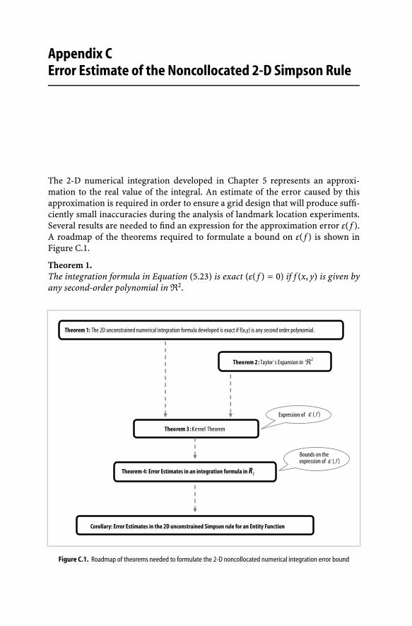
Appendix CError Estimate of the Noncollocated 2-D Simpson Rule
The 2-D numerical integration developed in Chapter 5 represents an approxi-mation to the real value of the integral. An estimate of the error caused by thisapproximation is required in order to ensure a grid design that will produce suffi-ciently small inaccuracies during the analysis of landmark location experiments.Several results are needed to find an expression for the approximation error ε( f ).A roadmap of the theorems required to formulate a bound on ε( f ) is shown inFigure C.1.
Theorem 1.The integration formula in Equation (5.23) is exact (ε( f ) = 0) if f (x, y) is given byany second-order polynomial inR2.
Figure C.1. Roadmap of theorems needed to formulate the 2-D noncollocated numerical integration error bound

130 Appendix C
Proof. Given the second-order polynomial f (x, y) = Ax2 + Bx + Cxy + Dy2 +Ey + F, the analytical integration formula in the interval
[xo + δL
x , xnx − δUx
] ×[yo + δL
y , yny − δUy
]is
xnx −δUx∫
xo+δLx
yny −δUy∫
yo+δLy
f (x, y) dy dx
=
xnx −δUx∫
xo+δLx
[Ax2y + Bxy + Cx
y2
2+ D
y3
3+ E
y2
2+ Fy
]yny −δUy
yo+δLy
dx
=A3
((yny − δU
y
)−(
yo + δLy
))((xnx − δU
x
)3−(xo + δL
x
)3)
+B2
((yny − δU
y
)−(
yo + δLy
))((xnx − δU
x
)2−(xo + δL
x
)2)
+C4
((yny − δU
y
)2−(
yo + δLy
)2)((
xnx − δUx
)2−(xo + δL
x
)2)
+D3
((yny − δU
y
)3−(
yo + δLy
)3) ((
xnx − δUx
)−(xo + δL
x
))
+E2
((yny − δU
y
)2−(
yo + δLy
)2) ((
xnx − δUx
)−(xo + δL
x
))
+ F((
yny − δUy
)−(
yo + δLy
)) ((xnx − δU
x
)−(xo + δL
x
)). (C.1)
We will prove that the integration formula in Equation (5.23) is exact for thesecond-order polynomial f (x, y) for the case of nx = ny = 2. The proof expands toany grid of [nx + 1]× [
ny + 1]
knots (according to Equations (5.18) and (5.21), nx
and ny are even numbers), since any square integration interval can be decomposedinto a tessellation of 3 × 3 knots.
Equation (5.23) can be written as:
∫ yf −δUy
yo+δLy
∫ xf −δUx
xo+δLx
f (x, y) dx dy =
hxhy
9
2∑i=0
2∑j=0
(Si,j − Ri,j(hx, hy, δL
x , δHx , δL
y , δHy ))
f (xi, yj) + ε( f ) , (C.2)
where
S =
⎡⎣
1 4 14 16 41 4 1
⎤⎦

Appendix C 131

132 Appendix C
and
f (xi, yj) = Ax2i + Bxi + Cxiyj + Dy2
j + Eyj + F
= A(
(2 − i)xo + ix2
2
)2
+ B(
(2 − i)xo + ix2
2
)
+ C(
(2 − i)xo + ix2
2
)((2 − j)yo + jy2
2
)(C.3)
+ D(
(2 − j)yo + jy2
2
)2
+ E(
(2 − j)yo + jy2
2
)+ F i, j ∈ {0, 1, 2} .
After algebraic manipulation we obtain:∫ yf −δU
y
yo+δLy
∫ xf −δUx
xo+δLx
f (x, y) dx dy =
A3
(xo + δL
x − x2 + δUx
)(x2o + 2δL
xxo +(δL
x
)2+ xox2 − δU
x xo
+ δLxx2 − δL
xδUx + x2
2 − 2δUx x2 +
(δU
x
)2
)(yo + δL
y − y2 + δUy
)
+B2
(xo + δL
x − x2 + δUx
) (xo + δL
x + x2 − δUx
) (yo + δL
y − y2 + δUy
)
+C4
(xo + δL
x − x2 + δUx
) (xo + δL
x + x2 − δUx
) (yo + δL
y − y2 + δUy
) (yo + δL
y + y2 − δUy
)
+D3
(yo + δL
y − y2 + δUy
)⎛⎝ y2o + 2δL
y yo +(
δLy
)2+ yoy2 − δU
y yo
+δLy y2 − δL
y δUy + y2
2 − 2δUy y2 +
(δU
y
)2
⎞⎠(xo + δL
x − x2 + δUx
)
+E2
(yo + δL
y − y2 + δUy
)(yo + δL
y + y2 − δUy
) (xo + δL
x − x2 + δUx
)
+ F(xo + δL
x − x2 + δUx
) (yo + δL
y − y2 + δUy
)
+ ε( f )
⇒∫ yf −δU
y
yo+δLy
∫ xf −δUx
xo+δLx
f (x, y) dx dy =
A3
((y2 − δU
y
)−(
yo + δLy
))((x2 − δU
x
)3−(xo + δL
x
)3)
+B2
((y2 − δU
y
)−(
yo + δLy
))((x2 − δU
x
)2−(xo + δL
x
)2)
+C4
((y2 − δU
y
)2−(
yo + δLy
)2)((
x2 − δUx
)2−(xo + δL
x
)2)
+D3
((y2 − δU
y
)3−(
yo + δLy
)3) ((
x2 − δUx
)−(xo + δL
x
))
+E2
((y2 − δU
y
)2−(
yo + δLy
)2) ((
x2 − δUx
)−(xo + δL
x
))
+ F((
y2 − δUy
)−(
yo + δLy
)) ((x2 − δU
x
)−(xo + δL
x
))
+ ε( f ) . (C.4)

Appendix C 133
Since Equation (C.1) is equal to Equation (C.4) for nx = ny = 2, this implies thatε( f ) = 0.
Theorem 1 is proven.
As for the 1-D case, Theorem 1 cannot be generalized for third-order polynomialsin R2 for the case where the integration interval is not coincidental with theintegration grid.
Definition 1. Let R2 ∈ R2 be a rectangle a ≤ x ≤ b, c ≤ y ≤ d.
Definition 2. The derivatives of f (x, y) will be written as follows:
f (i,j)(x, y) ≡ ∂i+j
∂xi∂yjf (x, y) i ≥ 0, j ≥ 0
f (0,0)(x, y) ≡ f (x, y)
f (i,j)(a, c) ≡ f (i,j)(x, y)∣∣
(x,y)=(a,c)
Definition 3. The selector function ψ(α, β, γ) is defined as:
ψ(α, β, γ) =
⎧⎨⎩
1 α ≤ β < γ−1 γ ≤ β < α
0 otherwise(C.5)
Theorem 2 (Taylor’s Series Expansion inR2 (from Stroud 1971)).If f (x, y) has the property that all the derivatives
f (i,j)(x, y) 0 ≤ i ≤ p 0 ≤ j ≤ q p ≥ 1 q ≥ 1
are defined and continuous in R2, then f (x, y) has the expansion
f (x, y) =p−1∑i=0
q−1∑j=0
(x − ao)i
i!( y − co) j
j!f (i,j)(ao, co)
+q−1∑j=0
( y − co) j
j!
x∫
ao
(x − u)p−1
(p − 1)!f (p,j)(u, co) du
+p−1∑i=0
(x − ao)i
i!
y∫
co
(x − v)q−1
(q − 1)!f (i,q)(ao, v) dv
+
x∫
ao
y∫
co
(x − u)p−1
(p − 1)!( y − v)q−1
(q − 1)!f (p,q)(u, v) du dv , (C.6)
where (ao, co) is any point of R2.
The proof of Theorem 2 is given in Chapter 5 of Stroud (1971).

134 Appendix C
Definition 4. Bp,q is the set (space) of all functions f (x, y) with the following prop-erties:
i. The derivative f (p,q)(x, y) is Riemann-integrable on R2
ii. The derivatives f (p,j)(x, co), j < q, are Riemann-integrable on a ≤ x ≤ b.iii. The derivatives f (i,q)(ao, y), i < p, are Riemann-integrable on c ≤ y ≤ d.iv. The derivatives f (i,j)(ao, co), i < p, j < q existv. Taylor’s expansion (Equation (C.6)) holds for f (x, y) for all (x, y) in R2
Theorem 3 (Kernel Theorem (from Stroud 1971)).Given an integration formula of the form
yf −δUy∫
yo+δLy
xf −δUx∫
xo+δLx
f (x, y) dx dy =∑
k
Akf (xk, yk) + ε( f ) , (C.7)
which is exact, in other words ε( f ) = 0 when f (x, y) is a polynomial of degree < pin x and degree < q in y, then there exist kernel functions:
Kp,q(x, y, ao, co) (x, y) ∈ R2 (ao, co) ∈ R2
Kp,j(x, ao, co) x ∈ [a, b] j < q
Ki,q( y, ao, co) y ∈ [c, d] i < p , (C.8)
so that
ε( f ) =q−1∑j=0
b∫
a
Kp,j(u, ao, co)f (p,j)(u, co) du
+p−1∑i=0
b∫
a
Ki,q(v, ao, co)f (i,q)(ao, v) dv
+
b∫
a
d∫
c
Kp,q(u, v, ao, co)f (p,q)(u, v) du dv (C.9)
whenever f (x, y) ∈ Bp,q(ao, co). Furthermore, the kernel functions in Equation (C.8)can be defined by
Kp,j(u, ao, co) = ε[
(x − u)p−1
(p − 1)!ψ(ao, u, x)
( y − co) j
j!
], u ∈ [a, b] 0 ≤ j < p
(C.10)
Ki,q(v, ao, co) = ε[
(x − ao)i
i!( y − v)q−1
(q − 1)!ψ(co, v, y)
], v ∈ [c, d] 0 ≤ i < q
(C.11)
Kp,q(u, v, ao, co) = ε[
(x − u)p−1
(p − 1)!ψ(ao, u, x)
( y − v)q−1
(q − 1)!ψ(co, v, y)
](u, v) ∈ R2 .
(C.12)

Appendix C 135
Proof. 1 The 2-D Taylor series expansion shown in Equation (C.6) has the form:
f (x, y) = Up−1,q−1(x, y) + Wp,q(x, y) , (C.13)
where Up−1,q−1(x, y) is a polynomial of degree < p in x and degree < q in y, andWp,q(x, y) represents the rest of the elements of the expansion; that is:
Up−1,q−1(x, y) =p−1∑i=0
q−1∑j=0
(x − ao)i
i!( y − co) j
j!f (i,j)(ao, co) (C.14)
Wp,q(x, y) =q−1∑j=0
( y − co) j
j!
x∫
ao
(x − u)p−1
(p − 1)!f (p,j)(u, co) du
+p−1∑i=0
(x − ao)i
i!
y∫
co
(x − v)q−1
(q − 1)!f (i,q)(ao, v) dv
+
x∫
ao
y∫
co
(x − u)p−1
(p − 1)!( y − v)q−1
(q − 1)!f (p,q)(u, v) du dv . (C.15)
From Equations (C.7) and (C.13), we can write:
yf −δUy∫
yo+δLy
xf −δUx∫
xo+δLx
f (x, y) dx dy
=
yf −δUy∫
yo+δLy
xf −δUx∫
xo+δLx
Up−1,q−1(x, y) dx dy +
yf −δUy∫
yo+δLy
xf −δUx∫
xo+δLx
Wp,q(x, y) dx dy
=∑
k
AkUp−1,q−1(xk, yk) +∑
k
AkWp,q(xk, yk) + ε( f ) ,
but since Up−1.q−1(x, y) is exact for degree < p in x and degree < q in y, this impliesthat:
yf −δUy∫
yo+δLy
xf −δUx∫
xo+δLx
Wp,q(x, y) dx dy =∑
k
AkWp,q(xk, yk) + ε( f )
or
ε( f ) =
yf −δUy∫
yo+δLy
xf −δUx∫
xo+δLx
Wp,q(x, y) dx dy −∑
k
AkWp,q(xk, yk) . (C.16)
1 This development is generalization of the proof presented in Stroud (1971).

136 Appendix C
Substituting the expression for Wp,q(x, y) into Equation (C.16) and rearrangingterms, we obtain:
ε( f ) =
yf −δUy∫
yo+δLy
xf −δUx∫
xo+δLx
⎡⎣
q−1∑j=0
( y − co) j
j!
x∫
ao
(x − u)p−1
(p − 1)!f (p,j)(u, co) du
⎤⎦dx dy
−∑
k
Ak
⎡⎣
q−1∑j=0
( yk − co) j
j!
x∫
ao
(x − u)p−1
(p − 1)!f (p,j)(u, co) du
⎤⎦
k
+
yf −δUy∫
yo+δLy
xf −δUx∫
xo+δLx
⎡⎣
p−1∑i=0
(x − ao)i
i!
y∫
co
(x − v)q−1
(q − 1)!f (i,q)(ao, v) dv
⎤⎦dx dy
−∑
k
Ak
⎡⎣
p−1∑i=0
(xk − ao)i
i!
y∫
co
( y − v)q−1
(q − 1)!f (i,q)(ao, v) dv
⎤⎦
k
+
yf −δUy∫
yo+δLy
xf −δUx∫
xo+δLx
⎡⎣
x∫
ao
y∫
co
(x − u)p−1
(p − 1)!( y − v)q−1
(q − 1)!f (p,q)(u, v) du dv
⎤⎦dx dy
−∑
k
Ak
⎡⎣
x∫
ao
y∫
co
(x − u)p−1
(p − 1)!( y − v)q−1
(q − 1)!f (p,q)(u, v) du dv
⎤⎦
k
.
Bringing out the summation of the i and j terms, we get:
ε( f ) =q−1∑j=0
yf −δUy∫
yo+δLy
xf −δUx∫
xo+δLx
⎡⎣
x∫
ao
( y − co) j
j!(x − u)p−1
(p − 1)!f (p,j)(u, co) du
⎤⎦dx dy
−q−1∑j=0
∑k
Ak
⎡⎣
x∫
ao
( yk − co) j
j!(xk − u)p−1
(p − 1)!f (p,j)(u, co) du
⎤⎦
k
+p−1∑i=0
yf −δUy∫
yo+δLy
xf −δUx∫
xo+δLx
⎡⎣
y∫
co
(x − ao)i
i!(x − v)q−1
(q − 1)!f (i,q)(ao, v) dv
⎤⎦dx dy
−p−1∑i=0
∑k
Ak
⎡⎣
y∫
co
(xk − ao)i
i!( yk − v)q−1
(q − 1)!f (i,q)(ao, v) dv
⎤⎦
k

Appendix C 137
+
yf −δUy∫
yo+δLy
xf −δUx∫
xo+δLx
⎡⎣
x∫
ao
y∫
co
(x − u)p−1
(p − 1)!( y − v)q−1
(q − 1)!f (p,q)(u, v) du dv
⎤⎦dx dy
−∑
k
Ak
⎡⎣
x∫
ao
y∫
co
(xk − u)p−1
(p − 1)!( yk − v)q−1
(q − 1)!f (p,q)(u, v) du dv
⎤⎦
k
. (C.17)
Using selector function ψ(α, β, γ), Equation (C.17) can be written as:
ε( f ) =q−1∑j=0
yf −δUy∫
yo+δLy
xf −δUx∫
xo+δLx
⎡⎣
b∫
a
( y − co) j
j!ψ(ao, u, x)
(x − u)p−1
(p − 1)!f (p,j)(u, co) du
⎤⎦dx dy
−q−1∑j=0
∑k
Ak
⎡⎣
b∫
a
( yk − co) j
j!ψ(ao, u, x)
(xk − u)p−1
(p − 1)!f (p,j)(u, co) du
⎤⎦
k
+p−1∑i=0
yf −δUy∫
yo+δLy
xf −δUx∫
xo+δLx
⎡⎣
d∫
c
(x − ao)i
i!(x − v)q−1
(q − 1)!ψ(co, v, y)f (i,q)(ao, v) dv
⎤⎦dx dy
−p−1∑i=0
∑k
Ak
⎡⎣
d∫
c
(xk − ao)i
i!( yk − v)q−1
(q − 1)!ψ(co, v, y)f (i,q)(ao, v) dv
⎤⎦
k
+
yf −δUy∫
yo+δLy
xf −δUx∫
xo+δLx
⎡⎣
b∫
a
d∫
c
(x − u)p−1
(p − 1)!ψ(ao, u, x)
( y − v)q−1
(q − 1)!ψ(co, v, y)
×f (p,q)(u, v) du dv
⎤⎦ dx dy
−∑
k
Ak
⎡⎣
b∫
a
d∫
c
(xk −u)p−1
(p−1)!ψ(ao, u, x)
( yk −v)q−1
(q−1)!ψ(co, v, y)f (p,q)(u, v) du dv
⎤⎦
k
.
Here the limits of integration (a, b, c, d) correspond to the boundaries of the rect-angle described in Definition 1. The order of the integration and summation canbe rearranged to give:
ε( f ) =q−1∑j=0
b∫
a
⎡⎢⎢⎢⎢⎢⎢⎣
yf −δUy∫
yo+δLy
xf −δUx∫
xo+δLx
( y − co) j
j!ψ(ao, u, x)
(x − u)p−1
(p − 1)!dx dy
−∑
k
Ak( yk − co) j
j!ψ(ao, u, x)
(xk − u)p−1
(p − 1)!
⎤⎥⎥⎥⎥⎥⎥⎦
f (p,j)(u, co) du

138 Appendix C
+p−1∑i=0
d∫
c
⎡⎢⎢⎢⎢⎢⎢⎣
yf −δUy∫
yo+δLy
xf −δUx∫
xo+δLx
(x − ao)i
i!( y − v)q−1
(q − 1)!ψ(co, v, y) dx dy
−∑
k
Ak(xk − ao)i
i!( yk − v)q−1
(q − 1)!ψ(co, v, y)
⎤⎥⎥⎥⎥⎥⎥⎦
f (i,q)(ao, v) dv
+
b∫
a
d∫
c
⎡⎢⎢⎢⎢⎢⎢⎣
yf −δUy∫
yo+δLy
xf −δUx∫
xo+δLx
(x − u)p−1
(p − 1)!ψ(ao, u, x)
( y − v)q−1
(q − 1)!ψ(co, v, y) dx dy
−∑
k
Ak(xk − u)p−1
(p − 1)!ψ(ao, u, x)
( yk − v)q−1
(q − 1)!ψ(co, v, y)
⎤⎥⎥⎥⎥⎥⎥⎦
× f (p,q)(u, v) du dv
or
ε( f ) =q−1∑j=0
b∫
a
Kp,j(u, ao, co)f (p,j)(u, co) du
+p−1∑i=0
d∫
c
Ki,q(v, ao, co)f (i,q)(ao, v) dv
+
b∫
a
d∫
c
Kp,q(u, v, ao, co)f (p,q)(u, v) du dv ,
where
Kp,j(u, ao, co) =
yf −δUy∫
yo+δLy
xf −δUx∫
xo+δLx
( y − co) j
j!ψ(ao, u, x)
(x − u)p−1
(p − 1)!dx dy
−∑
k
Ak( yk − co) j
j!ψ(ao, u, x)
(xk − u)p−1
(p − 1)!
Ki,q(v, ao, co) =
yf −δUy∫
yo+δLy
xf −δUx∫
xo+δLx
(x − ao)i
i!( y − v)q−1
(q − 1)!ψ(co, v, y) dx dy
−∑
k
Ak(xk − ao)i
i!( yk − v)q−1
(q − 1)!ψ(co, v, y)
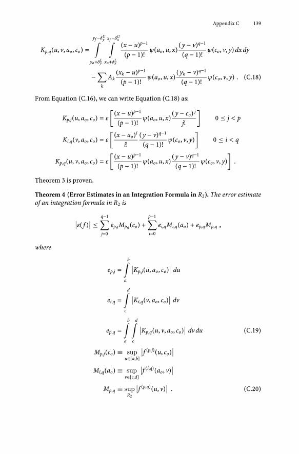
Appendix C 139
Kp,q(u, v, ao, co) =
yf −δUy∫
yo+δLy
xf −δUx∫
xo+δLx
(x − u)p−1
(p − 1)!ψ(ao, u, x)
( y − v)q−1
(q − 1)!ψ(co, v, y) dx dy
−∑
k
Ak(xk − u)p−1
(p − 1)!ψ(ao, u, x)
( yk − v)q−1
(q − 1)!ψ(co, v, y) . (C.18)
From Equation (C.16), we can write Equation (C.18) as:
Kp,j(u, ao, co) = ε[
(x − u)p−1
(p − 1)!ψ(ao, u, x)
( y − co) j
j!
]0 ≤ j < p
Ki,q(v, ao, co) = ε[
(x − ao)i
i!( y − v)q−1
(q − 1)!ψ(co, v, y)
]0 ≤ i < q
Kp,q(u, v, ao, co) = ε[
(x − u)p−1
(p − 1)!ψ(ao, u, x)
( y − v)q−1
(q − 1)!ψ(co, v, y)
].
Theorem 3 is proven.
Theorem 4 (Error Estimates in an Integration Formula in R2). The error estimateof an integration formula in R2 is
∣∣ε( f )∣∣ ≤
q−1∑j=0
ep,jMp,j(co) +p−1∑i=0
ei,qMi,q(ao) + ep,qMp,q ,
where
ep,j =
b∫
a
∣∣Kp,j(u, ao, co)∣∣ du
ei,q =
d∫
c
∣∣Ki,q(v, ao, co)∣∣ dv
ep,q =
b∫
a
d∫
c
∣∣Kp,q(u, v, ao, co)∣∣ dv du (C.19)
Mp,j(co) ≡ supu∈[a,b]
∣∣f (p,j)(u, co)∣∣
Mi,q(ao) ≡ supv∈[c,d]
∣∣f (i,q)(ao, v)∣∣
Mp,q ≡ supR2
∣∣f (p,q)(u, v)∣∣ . (C.20)

140 Appendix C
Proof. From Equation (C.9), we can write:
ε( f ) =q−1∑j=0
b∫
a
Kp,j(u, ao, co)f (p,j)(u, co) du +p−1∑i=0
b∫
a
Ki,q(v, ao, co)f (i,q)(ao, v) dv
+
b∫
a
d∫
c
Kp,q(u, v, ao, co)f (p,q)(u, v) du dv
∣∣ε( f )∣∣ ≤
∣∣∣∣∣∣∣∣∣
q−1∑j=0
b∫a
Kp,j(u, ao, co)f (p,j)(u, co) du +p−1∑i=0
b∫a
Ki,q(v, ao, co)f (i,q)(ao, v) dv
+b∫
a
d∫c
Kp,q(u, v, ao, co)f (p,q)(u, v) du dv
∣∣∣∣∣∣∣∣∣
≤∣∣∣∣∣∣
q−1∑j=0
b∫
a
Kp,j(u, ao, co)f (p,j)(u, co) du
∣∣∣∣∣∣+
∣∣∣∣∣∣
p−1∑i=0
b∫
a
Ki,q(v, ao, co)f (i,q)(ao, v) dv
∣∣∣∣∣∣
+
∣∣∣∣∣∣
b∫
a
d∫
c
Kp,q(u, v, ao, co)f (p,q)(u, v) du dv
∣∣∣∣∣∣
≤q−1∑j=0
b∫
a
∣∣Kp,j(u, ao, co)f (p,j)(u, co)∣∣ du +
p−1∑i=0
b∫
a
∣∣Ki,q(v, ao, co)f (i,q)(ao, v)∣∣ dv
+
b∫
a
d∫
c
∣∣Kp,q(u, v, ao, co)f (p,q)(u, v)∣∣ du dv
≤q−1∑j=0
b∫
a
∣∣Kp,j(u, ao, co)∣∣ ∣∣f (p,j)(u, co)
∣∣ du +p−1∑i=0
b∫
a
∣∣Ki,q(v, ao, co)∣∣ ∣∣f (i,q)(ao, v)
∣∣ dv
+
b∫
a
d∫
c
∣∣Kp,q(u, v, ao, co)∣∣ ∣∣f (p,q)(u, v)
∣∣ du dv
≤q−1∑j=0
b∫
a
∣∣Kp,j(u, ao, co)∣∣ sup
u∈[a,b]
∣∣f (p,j)(u, co)∣∣ du
+p−1∑i=0
b∫
a
∣∣Ki,q(v, ao, co)∣∣ sup
v∈[c,d]
∣∣f (i,q)(ao, v)∣∣ dv
+
b∫
a
d∫
c
∣∣Kp,q(u, v, ao, co)∣∣ sup
R2
∣∣f (p,q)(u, v)∣∣ du dv .

Appendix C 141
Defining
ep,j =b∫
a
∣∣Kp,j(u, ao, co)∣∣ du Mp,j(co) ≡ sup
u∈[a,b]
∣∣f (p,j)(u, co)∣∣
ei,q =d∫c
∣∣Ki,q(v, ao, co)∣∣ dv Mi,q(ao) ≡ sup
v∈[c,d]
∣∣f (i,q)(ao, v)∣∣
ep,q =b∫
a
d∫c
∣∣Kp,q(u, v, ao, co)∣∣ dv du Mp,q ≡ sup
R2
∣∣f (p,q)(u, v)∣∣ ,
we obtain:
∣∣ε( f )∣∣ ≤
q−1∑j=0
ep,jMp,j(co) +p−1∑i=0
ei,qMi,q(ao) + ep,qMp,q .
Theorem 4 is proven.
Corollary 1 (Error Estimates in the 2-D Noncollocated Simpson Rulefor an Illuminance Function).If f (x, y) = E(x, y) = G(x, y) ∗ H(x, y), where E(x, y) is the illuminance function,
G(x, y) = 12πσ2
be
− x2+y2
2σ2b is a 2-D Gaussian function representing the diffraction phe-
nomenon, and H(x, y) ∈ {0, …, 1} is the optical flux function, then the error estimateof the 2-D noncollocated Simpson rule is
∣∣ε( f )∣∣ ≤ hxhy
⎛⎝
2∑j=0
eN3,jM3,j +
2∑i=0
eNi,3Mi,3 + eN
3,3M3,3
⎞⎠ , (C.21)
where
eN3,j = e3,j
1hxhy
eNi,3 = ei,3
1hxhy
eN3,3 = e3,3
1hxhy
are normalized error coefficients (Stroud 1971) with e3,j, ei,3, e3,3 and M3,j, Mi,3, M3,3
defined as in Equations (C.19) and (C.20), respectively. Furthermore, the values ofthese coefficients are:
eN3,0 = eN
0,3 = 55.5 × 10⁻³
eN3,1 = eN
1,3 = 0
eN3,2 = eN
2,3 = 9.25 × 10⁻³
eN3,3 = 5.4167 × 10⁻³

142 Appendix C
and
M3,0 = M0,3 =1.380
s3b
M3,1 = M1,3 =0.837
s4b
M3,2 = M2,3 =1.380
s5b
M3,3 =1.9047
s6b
.
Proof. Given the results of Theorem 1 and Theorem 3, it can be easily concludedthat for the noncollocated Simpson rule p = q = 3.
The normalized error coefficients eN3,j, eN
i,3, eN3,3 are calculated using Theorem 4
and are tabulated in (Stroud 1971).The derivation of the coefficients M3,j, Mi,3, M3,3 follows:From the definition of an illuminance function we have:
E(x, y) = G(x, y) ∗ H(x, y) . (C.22)
Substituting Equation (C.22) into Equation (C.20), we obtain:
M3,j ≡ supu∈[a,b]
∣∣E(3,j)(u, co)∣∣ 0 ≤ j < 3
= supu∈[a,b]
∣∣∣∣∂3+j
∂u3∂vj
(G(x, y) ∗ H(x, y)
∣∣u=x,y=co
)∣∣∣∣
Mi,3 ≡ supu∈[a,b]
∣∣E(i,3)(ao, v)∣∣ 0 ≤ i < 3
M3,3 ≡ supu∈[a,b]
∣∣E(3,3)(u, v)∣∣ . (C.23)
The optical flux function that maximizes the convolution operation in Equa-tion (C.23) is H(x, y) = 1:
M3,j = supu∈[a,b]
∣∣∣∣∂3+j
∂u3∂vjG(u, v)|y=co
∣∣∣∣ 0 ≤ j < 3
Mi,3 = supu∈[a,b]
∣∣∣∣∂3+i
∂ui∂v3G(u, v)|x=ao
∣∣∣∣ 0 ≤ i < 3
M3,3 = supu∈[a,b]
∣∣∣∣∂3+3
∂u3∂v3G(u, v)
∣∣∣∣ . (C.24)
Calculating the supremum of the multiple Gaussian derivatives and substitutingin Equation (C.24), we get:

Appendix C 143
M3,0 = M0,3 =1.380
s3b
M3,1 = M1,3 =0.837
s4b
M3,2 = M2,3 =1.38
s5b
M3,3 =1.9047
s6b
.
The corollary is proven.
The corollary makes it easy to design the subsampling grid size, defined by hx
and hy. For a given desired maximum error∣∣e( f )
∣∣max ∈ 0, …, 1 and a smoothing
level sb determined by the camera system, using Equation (C.21) we can write:
hxhy =
∣∣ε( f )∣∣
max(2∑
j=0eN
3,jM3,j +2∑
i=0eN
i,3Mi,3 + eN3,3M3,3
) . (C.25)
For a squared subsampling grid, Equation (C.25) becomes:
hx = hy =
√√√√√√
∣∣ε( f )∣∣
max(2∑
j=0eN
3,jM3,j +2∑
i=0eN
i,3Mi,3 + eN3,3M3,3
) . (C.26)

Color Section
Plate 1. Landmarks use in the publishing and printed circuit board industries
Plate 2. Example locale maps for four values of fill factor and to levels of intensity quantization

146 Color Section
Plate 3. Effects of sensitive area, diffraction smoothing, and quantization
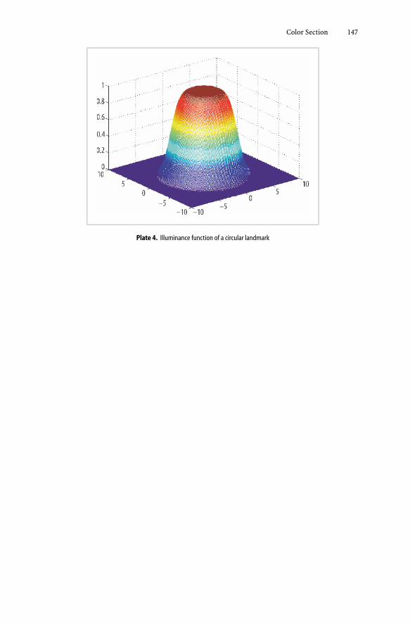
Color Section 147
Plate 4. Illuminance function of a circular landmark
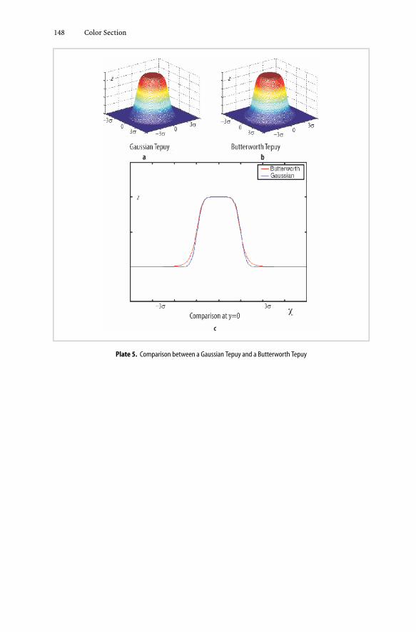
148 Color Section
Plate 5. Comparison between a Gaussian Tepuy and a Butterworth Tepuy
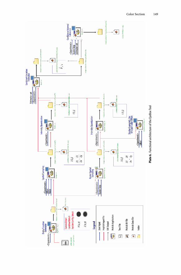
Color Section 149
Plat
e6.
Func
tiona
larc
hite
ctur
eof
the
EyeB
oxTo
ol

150 Color Section
Plate 7. Convolution of the optical flux function with a Gaussian Kernel to produce the illummance function

Color Section 151
Plat
e8.
Func
tiona
larc
hite
ctur
eof
the
EyeE
xpBo
xto
ol

152 Color Section
Plate 9. 18mm Configuration – Confidence Intervals – Constellation Details
Plate 10. 18mm Configuration – Confidence Intervals

Color Section 153
Plate 11. 35mm Configuration – Confidence Intervals

References
I. Amir, “An algorithm for finding the center of circular fiducials,” Computer Vision, Graphics, andImage Processing, Vol. 49, No. 1, pp. 398–406, 1990.
B. Armstrong, B.S. Holeman, “Target tracking with a network of Doppler radars,” IEEE Transactionson Aerospace and Electronic Systems, Vol. 34, No. 1, pp. 33–48, 1998.
B. Armstrong, T. Verron, L. Heppe, J. Reynolds, K. Schmidt, “RGR-3D: Simple, cheap detections of6-DOF pose for tele-operation, and robot programming and calibration.” In Proc. 2002 Int. Conf.on Robotics and Automation. IEEE: Washington, 2002.
K.B. Atkinson, “Close range photogrammetry and machine vision”, Caithness: Whittles Publishing,1996.
S. Baker, S. Nayar, H. Murase, “Parametric feature detection,” Proceedings of IEEE Conference on CVPR’96, San Francisco, CA, 16–20 June 1996, p. 471.
D.H. Ballard, “Generalizing the Hough transform to detect arbitrary shapes,” Pattern Recognition,Vol. 13, No. 2, pp. 111–122, 1981.
C.B. Bose, I. Amir, “Design of fiducials for accurate registration using machine vision,” IEEE Transac-tions on Pattern Analysis and Machine Intelligence, Vol. 12, No. 12, pp. 1196–1200, 1990.
C.A. Berenstein, L.N. Kanal, D. Lavine, E.C. Olson, “A geometric approach to subpixel registrationaccuracy,” Computer Vision, Graphics, and Image Processing, Vol. 40, No. 3, pp. 334–336, 1987.
A.M. Bruckstein, “On optimal image digitalization,” IEEE Transactions on Acoustics, Speech, and SignalProcessing, Vol. 35, No. 4, pp. 553–555, 1987.
A.M. Bruckstein, L. O’Gorman, A. Orlitsky, “Design of shapes for precise image registration,” IEEETransactions on Information Theory, Vol. 44, No. 7, pp. 3156–3162, 1998.
A.M. Bruckstein, R.J. Holt, “Optimum fiducials under weak perspective projections,” Proceedings of the7th IEEE International Conference on Computer Vision, Kerkyra, Vol. 1, No. 1, 20–27 September1999.
G. Chiorboli, G.P. Vecchi, Comments on “Design of fiducials for accurate registration using machinevision,” IEEE Transactions on Pattern Analysis and Machine Intelligence, Vol. 15, No. 12, pp. 1330–1332, 1993.
I.J. Cox, J.B. Kruskal, D.A. Wallach, “Predicting and estimating the accuracy of a subpixel registrationalgorithm,” IEEE Transactions on Pattern Analysis and Machine Intelligence, Vol. 12, No. 8, pp. 721–734, 1990.
J.J. Craig, “Introduction to robotics,” Reading, MA: Addison–Wesley, 1986.M. Doros, “On the properties of the generation of discrete circular arcs on a square grid,” Computer
Vision, Graphics, and Image Processing, Vol. 28, No. 1, pp. 377–383, 1984.L. Dorst, A.W.M. Smeulders, “Best linear unbiased estimators for properties of digitized straight lines,”
IEEE Transactions on Pattern Analysis and Machine Intelligence, Vol. 8, No. 2, pp. 279–282, 1986.R.O. Duda, P.E. Hart, “Use of Hough transformation to detect lines and curves in pictures,” Communi-
cations of the ACM, Vol. 15, No. 1, pp. 11–15, 1972.V.N. Dvornychenko, “Bound on (deterministic) correlation functions with application to registration,”
IEEE Transactions on Pattern Analysis and Machine Intelligence, Vol. 5, No. 2, pp. 206–213, 1983.A. Efrat, C. Gotsman, “Subpixel image registration using circular fiducials,” International Journal on
Computational Geometry and Applications, Vol. 4, No 4, pp. 403–422, 1994.
156 References
W. Förstner, “On the geometric precision of digital correlation,” Proceedings of the InternationalArchives of Photogrammetry and Remote Sensing (ISPRS) Commun. III Symp., Helsinki, Vol. 24,No. 3, pp. 176–189, 1982.
J. Goodman, “Introduction to Fourier optics,” New York: McGraw–Hill Inc., 1968.R.A. Gonsalves, “Cramér–Rao bounds on mensuration errors,” Applied Optics, Vol. 15, No. 5, pp. 1270–
1275, 1976.R.C. Gonzalez, R.E. Woods, “Digital image processing,” Boston: Addison–Wesley Publishing Company,
1992.A. Hachicha, S. Simon, K. Hanna, “The use of gray-level information and fitting techniques for precise
measurement of corneal curvature and thickness,” Computer Vision and Pattern Recognition,Vol. 47, No. 1, pp. 131–164, 1989.
J. Hair, R. Anderson, R. Tatham, W. Black, “Multivariate data analysis with readings,” 3rd edn., NewYork: Macmillan Publishing Company, 1992.
D.I. Havelock, “Geometric precision in noise-free digital images,” IEEE Transactions on Pattern Analysisand Machine Intelligence, Vol. 11, No. 10, pp. 1065–1075, 1989.
D.I. Havelock, “The topology of locales and its effects on position uncertainty,” IEEE Transactions onPattern Analysis and Machine Intelligence, Vol. 13, No. 4, pp. 380–386, 1991.
M. Heath, S. Sarkar, T. Sanocki, K. Bowyer, “Comparison of edge detectors: a methodology and initialstudy,” Proceedings of the 1996 IEEE Conference CVPR ’96, San Francisco, CA, 16–20 June 1996,pp. 143–148.
E. Hecht, A. Zajac, “Optics,” Boston: Addison–Wesley Publishing Company, 1979.J.W. Hill, “Dimensional measurements from quantized images,” in: D. Nitzan et al., “Machine intelli-
gence research applied to industrial automation,” SRI 10th Report for NSF Grant DAR78-27128,Washington, DC: National Science Foundation, pp. 75–105, 1980.
C.-S. Ho, “Precision of digital vision systems,” IEEE Transactions on Pattern Analysis and MachineIntelligence, Vol. 5, No. 6, pp. 593–601, 1983.
P.D. Hyde, L.S. Davis, “Subpixel edge estimation,” Pattern Recognition, Vol. 16, No. 4, pp. 413–420, 1983.H. Hung, “Lower bound on average mean-square error for image restoration,” IEEE Transactions on
Signal Processing, Vol. 39, No. 2, pp. 497–499, 1991.IEEE SA, “IEEE 100, The authoritative dictionary of IEEE standard terms,” 7th edn, Los Alamitos, CA:
IEEE Press, 2000.B. Jahne, “Practical handbook on image processing for scientific applications,” Boca Raton, FL: CRC
Press, 1997.S.M. Kay, “Fundamentals of statistical signal processing: estimation theory,” Upper Saddle River, NJ:
Prentice–Hall, 1993.N. Kiryati, A. Bruckstein, “Gray-levels can improve the performance of binary image digitizers,” Com-
puter Vision and Pattern Recognition, Vol. 53, No. 1, pp. 31–39, 1991.H. Klaasman, “Some aspects of the accuracy of the approximated position of a straight line on a square
grid,” Computer Vision, Graphics, and Image Processing, Vol. 4, No.1, pp. 225–235, 1975.A. Krommer, C.W. Ueberhuber, “Computational integration,” Philadelphia, PA: Society for Industrial
and Applied Mathematics Press, 1998.Z. Kulpa, “On the properties of discrete circles, rings, and disks,” Computer Vision, Graphics, and
Image Processing, Vol. 10, No. 1, 1979, pp. 348–365.C.R. McCluer, “Industrial mathematics: modeling in industry, science, and government,” Upper Saddle
River, NJ: Prentice–Hall, 2000.A. Nakamura, K. Aizawa, “Digital circles,” Computer Vision, Graphics, and Image Processing, Vol. 26,
No. 1, pp. 242–255, 1984.V.S. Nalwa, T.O. Binford, “On detecting edges,” IEEE Transactions on Pattern Analysis and Machine
Intelligence, Vol. 8, No. 6, pp. 699–714, 1986.L. Nielsen, K. Astrom, E. Jury, “Optimal digitization of 2-D images,” Transactions on Acoustics, Speech,
and Signal Processing, Vol. 32, No. 6, pp. 1247–1249, 1984.H.K. Nishihara, P.A. Crossley, “Measuring photolithographic overlay accuracy and critical dimensions
by correlating binarized Laplacian and Gaussian convolution,” IEEE Transactions on PatternAnalysis and Machine Intelligence, Vol. 10, No. 1, pp. 17–30, 1988.
References 157
L. O’Gorman, A.M. Bruckstein, C.B. Bose, I. Amir, “Subpixel registration using concentric ring fiducial,”Proceedings of the 10th International Conference on Pattern Recognition, Atlantic City, NJ, 16–21June 1990, pp. 249–253.
L. O’Gorman, “Subpixel precision of straight-edged shapes for registration and measurement,” IEEETransactions on Pattern Analysis and Machine Intelligence, Vol. 18, No. 7, pp. 746–751, 1996.
P.Z. Peebles, “Probability, random variables, and random signal principles,” 4th edn., New York:McGraw–Hill Inc., 2001.
J.G. Proakis, D.G. Manolakis, “Digital signal processing: principles, algorithms, and applications,”3rd edn., Upper Saddle River, NJ: Prentice–Hall, 1996.
A. Reza, M. Doroodchi, “Cramér–Rao lower bound on locations of sudden changes in a steplike signal,”IEEE Transactions on Signal Processing, Vol. 44, No. 16, pp. 2551–2556, 1996.
D. Robinson, P. Milanfar, “Fundamental performance limits in image registration,” IEEE Transactionson Image Processing, Vol. 13, No. 9, pp. 1185–1199, 2004.
K. Rohr, “Landmark-based image analysis: using geometric and intensity models,” Amsterdam: KluwerAcademic Publishers, 2001.
T.W. Ryan, R.T. Gray, B.R. Hunt, “Prediction of correlation errors in stereopairs images,” OpticalEngineering, Vol. 19, No. 3, pp. 312–322, 1982.
L.L. Scharf, “Statistical signal processing, detection, estimation, and time series analysis,” Boston, MA:Addison–Wesley Publishing Company, 1990.
L.L. Scharf, L.T. McWhorter, “Geometry of the Cramér–Rao bound,” Signal Processing, Vol. 31, No. 3,pp. 1–11, 1993.
F.W. Sears, “Optica,” Boston, MA: Addison–Wesley, 1979.S.D. Shapiro, “Properties of transforms for the detection of curves in noisy pictures,” Computer Graphics
and Image Processing, Vol. 8, No. 1, pp. 219–236, 1978.R. Sriraman, J. Koplowitz, S. Mohan, “Tree searched chain coding for subpixel reconstruction of planar
curves,” IEEE Transactions on Pattern Analysis and Machine Intelligence, Vol. 11, No. 1, pp. 95–104,1989.
S. Stewart, “Calculus: early transcendentals,” Pacific Grove, CA: Brooks/Cole Publishing Co., 1994.A.H. Stroud, “Approximate calculation of multiple integrals,” Upper Saddle River, NJ: Prentice-Hall,
1971.A.J. Tabatabai, O.R. Mitchell, “Edge detection to subpixel values in digital imagery,” IEEE Transactions
on Pattern Analysis and Machine Intelligence, Vol. 6, No. 2, pp. 181–201, 1984.J.D. Thurgood, M.E. Mikhail, “Photogrammetric analysis of digital images,” International Archives of
Photogrammetry, Vol. 24, No. 3, pp. 576–590, 1982.Q. Tian, M.N. Huhns, “Algorithms for subpixel registration,” Computer Vision, Graphics, and Image
Processing, Vol. 35, No. 2, pp. 220–233, 1986.M. Tichem, M.S. Cohen, “Sub-μm registration of fiducial marks using machine vision,” IEEE Transac-
tions on Pattern Analysis and Machine Intelligence, Vol. 16, No. 8, pp. 791–794, 1994.H.L. Van Trees, “Detection, estimation, and modulation theory, Part 1,” New York: John Wiley & Sons,
Inc., 1968.A.M. Vossepoel, A.W.M. Smeulders, “Vector code probability and metrication error in the representa-
tion of straight lines of finite length,” Computer Vision, Graphics, and Image Processing, Vol. 20,No. 1, pp. 347–364, 1982.
B. Widrow, “A study of rough amplitude quantization by means of Nyquist sampling theory,” IRETransactions on Circuit Theory, Vol. 3, No. 1, pp. 266–276, 1965.
S. Yam, L.S. Davis, “Image registration using generalized Hough transforms,” Proceedings of IEEEComputer Society on Pattern Recognition and Image Processing, Dallas, TX, 3–5 August 1981, pp.526–533.
J. Zheng, M. Lei, “Method and apparatus for locating an acquisition target in two-dimensional imagesby detecting symmetry in two different directions,” United States Patent 5,515,447, 1996.
J.Y. Zhou, D. Lopresti, P. Sarkar, G. Nagy, “Spatial sampling effects on scanned 2-D patterns,” IEEETransactions on Pattern Analysis and Machine Intelligence, Vol. 20, No. 3, 1998.
R.E. Ziemmer, W.H. Tranter, D.R. Fannin, “Signals and systems: continuous and discrete,” New York:Macmillan Publishing Co., 1983.

Index
1-D Simpson rule 702-D Gaussian 812-D Simpson rule 512-D integration 33, 462-D sampling 34, 363-D integration 564-D integration 49
aberrations 32adjusted focal length 32Airy disk 31, 32, 123Airy pattern 30, 125amplitude quantization 5analog intensity 38analog intensity function 23, 38
discrete 26, 39, 51, 84, 125apodization 31artificial landmarks 3artwork 90aspect ratio
pixel 115autocorrelation 5, 11
Bessel function 30binary algorithm 12binary centroid estimators 84, 87binary images 10blurring 32box pattern 92Butterworth tepuy estimator 14, 57, 60, 63, 84,
86, 87, 100, 148
calibration vii, 94camera
aperture 30Camera Calibration 94camera calibration 3, 94, 97Camera coordinates 15camera frame 16centroid 5, 28, 35, 92
algorithm 14, 59, 125
circular landmark 10, 21, 56, 60, 79, 87, 105component alignment 1computational cost 100confidence interval 11, 13, 43, 49, 50, 54, 79, 85,
86, 97, 99, 100, 104–106, 109, 121, 152, 153maps 87, 104
configurations 13contour interpolation algorithm 58convolution 14, 33convolution operator 31coordinate frames 15correlation methods 8covariance matrix 42, 55covariance uncertainty 49Cramér–Rao lower bound 4, 11, 14, 24, 45, 48,
58, 65, 79, 82, 85–87, 104, 105, 109, 110, 118,121, 125
cubature formulae 66
dark current noise 97decentering 33defocus 11, 32, 44, 58, 110diffraction 11, 14, 23, 30, 43, 58, 60, 81, 103,
105, 110, 123, 125, 146digital circles 10digital image 4, 24, 26, 39, 45, 51, 59, 84, 123,
125ideal 50
discrete analog intensity function 17, 21, 46distortion model 34Doppler radar tracking 45dynamic range 103
ellipsoid model 58ellipsoidal contour algorithm 14, 57, 63, 84, 87,
100, 122estimation processes 4estimator 19
bias 11, 28, 42, 54biased 48binary centroid 19, 98–100, 109Butterworth tepuy 19, 61, 99, 100, 109
160 Index
centroid 44, 100, 101confidence interval 56, 82covariance 42, 55ellipsoidal contour 19, 61, 99, 100, 109gray-scale 109grayscale centroid 19, 99, 100model-based 60, 101, 115, 118nano-triangles 89, 91, 93, 98, 101, 104practical 11unbiased 48uncertainty 23, 55
experimental validation 4extensive model of image formation 11EyeBox 79EyeCI 85EyeEntity 79EyeExpBox 97EyeExpConfig 97EyeExpDisk 98EyeQi 84EyeQs 82EyeRasterQi 84EyeRasterQs 82EyeT 84
Fiducial marks 1, 125fill factor 24, 38, 41, 126, 145finite support 28Fisher information matrix 47, 48fitting 51focal length 32focal number 32Fourier optics 26
Gaussian diffraction kernel 60Gaussian distribution 32Gaussian kernel 23, 31Gaussian noise 39Gaussian tepuy 60geometric optics 17geometrical algorithm 12geometrical analysis 10gray level 10, 126
information 11grayscale 126
centroid 84, 87contour 14image 12information 11
high-resolution grid 65Hough transforms 5Huygens–Fresnel principle 30
illuminance function 14, 17, 25, 31, 33–35, 46,60, 65, 66, 79, 82, 123, 125, 126, 141, 142,147, 150
image 103acquisition 28binary digital 10coordinates 18digital 17, 18, 37formation 79, 121, 126noise 6, 27, 41, 96, 103, 109principal point 81, 127Quantization 4synthetic 10, 43unquantized 10
image acquisition artifacts 12image acquisition systems
optical flux function 28image coordinates 15image formation 10, 11, 16, 21, 28image metrology 1, 3
applications 1image processing 12image restoration 45image setter 89image system 12image-guided surgery 1imaging processes 11impulsive 28inertial coordinate system 15integrated circuit manufacturing 5integration error 66intensity level 3, 61, 92intensity quantization 10, 21, 24, 38, 39, 54intensity quantization function 18
knots 65
Lagrange basis functions 68Lagrange interpolation polynomials 67landmark 4, 24
artificial 1, 2bull’s eye 29design 12detected 4diamond 29Geometry 6, 29image 21luminosity function 17, 25pose 16, 28size 12, 112square 29starbust 29tilt 28, 113
landmark coordinates 15landmark location 3

Index 161
bias 34covariance 52error 99–101estimation 84estimator error 87precision 21statistical analysis 5subpixel 5, 11subpixel accuracy 3, 4true 41uncertainty 5, 10, 11, 28, 29, 103, 104, 109
landmark location performance 14landmark plane 17landmark shapes 29lens calibration 94lens distortion 4, 33, 84lens law 32linear covariance approximation 53locale 10, 34, 38, 40, 118, 126locale map 40, 41, 145locale phenomenon 119location estimation algorithms 4location uncertainty 5luminosity dynamic range 111
machine vision 5many-to-one mapping 10MATLAB 79medical images 2millipixels 14minimum uncertainty 3mobile robot navigation 1model-based
estimators 110modulation transfer function 94, 126Monte Carlo integration 51, 56Monte Carlo sample 99Monte Carlo sampling 89, 99multimode imaging 1
Nalwa–Binford algorithm 57, 90, 122nano-triangles estimator 122Newton–Raphson method 57, 59, 61, 63nitrogen molecule 93noise model 39noise-free 42noncollocated 65nonlinear estimation 59nonuniform illumination 12, 28, 81, 89, 92,
103, 105, 116numerical analysis 14numerical integration 46, 51, 65, 66, 82, 86, 129
approximation error 77Simpson’s rule 50
numerical stability 66
object tracking 1optical bench 89optical flux function 17, 25, 46, 79, 123, 126,
141, 142, 150optics systems 12Origin of the Coordinate System 16
parametric modeling 5, 8performance map 13, 43, 103, 106perspective distortion 28photogrammetry 1–3, 5, 113, 125, 127Photomodeler 94photosensitive area 28physics of image formation 4pinhole model 79pitch 81pixel 3, 65, 114, 127
aspect ratio 114coordinates 18finite sensitive area 21geometry 11sensitive area 11, 14, 23, 57, 82, 114
pixel coordinates 15precision edge location 5principal distance 31, 81, 125, 127principal point 31printed circuit board 5probability density function 49product formula 66propagation number 30
quadratic interpolation 67quantization 146
amplitude 17, 46, 84, 89, 103, 117, 123error 39intensity 40, 145processes 4resolution 118spatial 17, 40
Qunatization Intensity 6
radial probability density function 55recursive induction 53resolution 5robotic manipulation 3roll 81
scene properties 12sensitive area 14, 22, 24, 34, 36, 38–41, 43, 44,
58, 65, 66, 81, 89, 103, 114, 115, 121, 127,146
Simpson rule 66six degree-of-freedom 11skew error 36

162 Index
smoothing 23, 24, 30, 32, 33, 143, 146effects 7illuminance function 21operator 46parameter 81radius 57, 103, 114
smoothing image 14smoothing radius 110, 115spatial measurement 2spatial partial derivatives 45spatial sampling 12, 34, 123spatial sampling density 5spatially quantized 24statistical analysis 5statistical modeling 8statistics
nonstationary 4, 24, 41, 43, 46, 51, 106Steacie Institute for Molecular Sciences 93step-like signals 45
synthetic images 5
table mountain 57Taylor series expansion 52, 53tepuy 57tilt 103
uncertaintysources of 4
UV-cure 89
values 21
wavelength 32Whittaker–Shannon sampling theorem 34World coordinates 15
yaw 81