Precipitation in Boreal Summer Simulated by a GCM with Two

Precipitation in Boreal Summer Simulated by a GCM with Two ConvectiveParameterization Schemes: Implications of the Intraseasonal

Oscillation for Dynamic Seasonal Prediction

SUHEE PARK

National Institute of Meteorological Research, Korea Meteorological Administration, Seoul, South Korea

SONG-YOU HONG

Department of Atmospheric Sciences, and Global Environment Laboratory, Yonsei University, Seoul, South Korea

YOUNG-HWA BYUN

National Institute of Meteorological Research, Korea Meteorological Administration, Seoul, South Korea

(Manuscript received 3 June 2009, in final form 20 November 2009)

ABSTRACT

In this paper, the intraseasonal oscillation (ISO) and its possible link to dynamical seasonal predictability

within a general circulation model framework is investigated. Two experiments with different convection

scheme algorithms, namely, the simplified Arakawa–Schubert (SAS) and the relaxed Arakawa–Schubert

(RAS) convection algorithms, were designed to compare seasonal simulations from 1979 to 2002 on a seasonal

model intercomparison project (SMIP)-type simulation test bed. Furthermore, the wave characteristics (wave

intensity, period, and propagation) of the simulated ISO signal provided by the model with two different

convection schemes for extended boreal summers from 1997 to 2004 were compared to the observational ISO

signal. Precipitation in the boreal summer was fairly well simulated by the model irrespective of the convection

scheme used, but the RAS run outperformed the SAS run with respect to tabulated skill scores. Decomposition

of the interannual variability of boreal summer precipitation based on observations and model results dem-

onstrates that the seasonal predictability of precipitation is dominated by the intraseasonal component over the

warm pool area and the SST-forced signal over the equatorial Pacific Ocean, implying that the seasonal mean

anomalies are more predictable under active ISO conditions as well as strong ENSO conditions. Comparison of

the ISO simulations with the observations revealed that the main features, such as the intensity of precipitation

variance in the intraseasonal time scale and the evolution of propagating ISOs, were reproduced fairly well by

the model; however, the wave characteristics associated with the ISO signals were better captured by the

experiment with the RAS scheme than the SAS scheme. This study further suggests that accurate simulation of

the ISO can improve the seasonal predictability of dynamical seasonal prediction systems.

1. Introduction

Prediction of seasonal mean climate is one of the chal-

lenges of climate prediction (e.g., Anderson et al. 1999;

Shukla et al. 2000). Many studies have developed models

for seasonal prediction based on a statistical, dynamical,

or a hybrid approach combining statistical and dynamical

methods. The statistical method takes into account certain

indices associated with low-frequency components of the

climate systems. Statistical models have shown reasonable

skill when the seasonal mean lies close to the norm, but

have little skill in predicting extreme events such as the

severe drought of the 2002 Indian monsoon (Goswami

et al. 2006). Furthermore, it is difficult to provide a com-

plete physical description of seasonal climate anomalies

predicted by statistical models. Meanwhile, the dynamic

approach, which is based on general circulation models

(GCMs) (Kumar et al. 1996; Shukla et al. 2000) and

global–regional coupled dynamical downscaling models

(Nobre et al. 2001; Sun et al. 2006), makes it possible to

provide mechanisms for the evolution of climate anomalies

Corresponding author address: Dr. Song-You Hong, Dept. of

Atmospheric Sciences, College of Science, Yonsei University,

Seoul 120-749, South Korea.

E-mail: [email protected]

15 MAY 2010 P A R K E T A L . 2801

DOI: 10.1175/2010JCLI3283.1

� 2010 American Meteorological SocietyUnauthenticated | Downloaded 01/16/22 06:04 AM UTC

in response to slowly varying external forcing. The hy-

brid statistical–dynamical approach applies statistical

methods to the past performance of a dynamic model

(Graham and Barnett 1995; Mo and Straus 2002).

An example of a dynamic model for seasonal prediction

is the fully coupled ocean–land–atmosphere dynamical

seasonal model that the National Centers for Environ-

mental Prediction (NCEP) has used to issue operational

seasonal forecasts since 2004 (Saha et al. 2006). This

dynamical modeling system has shown a better level

of skill in forecasting U.S. surface temperature and pre-

cipitation than statistical methods. In addition, European

researchers have an active seasonal-to-interannual pre-

diction project, known as the Development of a European

Multimodel Ensemble System for Seasonal to Interannual

Prediction (DEMETER; Palmer et al. 2004). Seven global

atmosphere–ocean coupled models are included in this

project and seasonal ensemble forecasts are used for crop

yield prediction. However, despite successful application

of the GCM to seasonal prediction in some regions (e.g.,

North America and Europe), dynamical prediction does

not yet guarantee overall better skill than the statistical

approach (Barnston et al. 2003).

The present skill of dynamical seasonal prediction is

limited by several factors, mainly the inherently nonlinear

characteristics of the atmosphere and the inaccuracy of

current GCMs (Anderson et al. 1999; Barnston et al.

2003), particularly over the Asian monsoon region (Kang

et al. 2004; Goswami et al. 2006). It has become clear that

external forcing, especially slowly varying anomalous

lower boundary forcing, is more important than infor-

mation from the atmospheric initial state for predicting

anomalous atmospheric circulation features on time scales

beyond a month or season. To address this, dynamical sea-

sonal prediction is based on the fact that slowly varying

boundary conditions, such as sea surface temperature

(SST) and snow cover, affect mainly global atmospheric

circulation and surface climate.

Meanwhile, the tropical intraseasonal oscillation (ISO),

also known as the Madden–Julian oscillation (MJO), is

the most important variability at the subseasonal time

scale, and is a dominant mode in the tropical region with

eastward periods of 30–60 days (Madden and Julian

1994). Several studies have reported that the ISO has an

influence on large-scale circulation and precipitation over

the subtropical and extratropical regions (e.g., Kang et al.

1989; Jones et al. 2004; Liess et al. 2005; Lorenz and

Hartmann 2006; Kim et al. 2006). Kang et al. (1989)

showed that the observational ISO anomaly, which starts

in the tropical Indian Ocean and ends south of Japan, is

closely related to variation in the East Asian summer

monsoon. Jones et al. (2004) examined the importance of

the MJO in the Northern Hemisphere weather forecasts,

and demonstrated that the MJO signal is important in

modulating weather variability. Liess et al. (2005) ana-

lyzed the upper limit of potential predictability of the

northern summer ISO, and found that the predictability

follows the eastward- and northward-propagating ISO

during the active and break phases of the Asian monsoon.

The analysis of Lorenz and Hartmann (2006) demon-

strated that the MJO could affect the North American

monsoon by modulating low-level circulation. Kim et al.

(2006) found that the eastward-moving upper-level di-

vergence over an active tropical convective area has a

subtropical counterpart in the upper-level divergence

region of the MJO, and deduced that vorticity advection

by vertical motion and the tilting of vorticity are sources

of midlatitude–MJO teleconnection. As reviewed by

Sperber and Waliser (2008), it is clear that the MJO has

wide-ranging impacts on the atmosphere–ocean–land

system, including Asian–Australian monsoon variabil-

ity, tropical cyclone activity, and weather patterns in the

extratropics. It is therefore very important to under-

stand, simulate, and forecast the MJO in climate models

and numerical weather forecast models.

In the present study, we examine the relation between

the seasonal mean of boreal summer climate and the

embedded ISO signal, both of which are simulated by

a GCM. The cumulus convection scheme is known to

have an important role in ISO simulation because the

coupling between convection and circulation is a key

process in the MJO (e.g., Wang and Schlesinger 1999; Lee

et al. 2003; Zhang and Mu 2005) and seasonal mean cli-

mate (e.g., Gregory et al. 1997; Donner et al. 2001; Byun

and Hong 2007). Therefore, in this study, we compare

seasonal simulations with two different cumulus convec-

tion schemes in a GCM, focusing on the seasonal mean

precipitation and a possible contribution of the ISO to the

seasonal mean. It is important to note that the purpose of

our study is not to judge the superiority of one scheme

over the other in simulating climatology, but rather to

identify a possible link between the ISO and the seasonal

mean climate. The experimental design and model de-

scription are presented in section 2. The skill of seasonal

simulations with two difference convection schemes is

presented in section 3, together with the simulated mean

ISO component embedded in the interannual variability

in precipitation. The characteristics of the simulated ISO

are discussed further in section 4. Summary statements

and concluding remarks are provided in section 5.

2. Model and experimental design

a. Model description

The atmospheric model used in this study is a version of

the NCEP Medium-Range Forecast (MRF) model with

2802 J O U R N A L O F C L I M A T E VOLUME 23

Unauthenticated | Downloaded 01/16/22 06:04 AM UTC

the physics package that was operational as of January

2000 (Kanamitsu et al. 2002a). The model employs a

horizontal resolution with spectral truncations of T62

(triangular truncation of wavenumbers at 62, roughly

corresponding to about 200 km) and a 28-layer terrain-

following sigma coordinate in the vertical dimension.

Model physics include long- and shortwave radiation,

cloud–radiation interaction, planetary boundary layer

processes, deep and shallow convection, large-scale con-

densation, gravity wave drag, simple hydrology, and ver-

tical and horizontal diffusions.

Two different cumulus parameterizations for deep

convection were utilized to conduct sensitivity experi-

ments. One was the simplified Arakawa–Schubert (SAS)

scheme (Pan and Wu 1995), which is in turn based on

Arakawa and Schubert (1974), as simplified by Grell

(1993) with a saturated downdraft. The other convection

scheme selected for this study was the relaxed Arakawa–

Schubert (RAS) scheme (Moorthi and Suarez 1992),

which was implemented in the recent NCEP seasonal

forecast model (Kanamitsu et al. 2002a). The main dif-

ferences between SAS and RAS lie in two components:

the clouds model and the treatment of downdrafts. The

SAS allows only one type of cloud, while RAS allows

a cloud ensemble with different tops; the SAS considers

saturated downdrafts based on empirical formulation,

which is absent in the current version of the RAS scheme.

These differences result in different precipitation pat-

terns and vertical heating and moistening profiles (Byun

and Hong 2004). Kanamitsu et al. (2002a) showed that

the RAS parameterization scheme performs better than

the SAS scheme with respect to the Pacific–North Amer-

ica (PNA) pattern in response to an idealized SST forcing

over the equatorial Pacific. For short- and medium-range

forecasts, the SAS has demonstrated good skill in pre-

dicting tropical precipitation (Kalnay et al. 1996).

b. Experimental design

First, Seasonal Model Intercomparison Project (SMIP)-

type experiments were performed using observed SST

data (Reynolds and Smith 1994). These experiments are

referred to ‘‘EXP-SAS’’ and ‘‘EXP-RAS’’ for runs with

the SAS and RAS schemes, respectively. Both integra-

tions were carried out with an approximate 4-week lead

time for the boreal summer [June–August (JJA)] over

a 24-yr period, from 1979 to 2002. Each experiment had

10-member ensembles. Initial conditions were taken

from the NCEP/Department of Energy (DOE) Global

Reanalysis 2 data (Kanamitsu et al. 2002b), starting from

0000 UTC 26 April and running to 30 April, with a 12-h

interval. Observed monthly precipitation data from the

Climate Prediction Center (CPC) Merged Analysis of

Precipitation (CMAP) data (Xie and Arkin 1997) were

used to evaluate the modeled precipitation. This set of

experiments was performed to evaluate seasonal precipi-

tation and the intraseasonal component of the total inter-

annual variability of precipitation simulated by the model.

Similar to the SMIP-type run, two integrations with

the SAS and RAS cumulus parameterization schemes

were conducted for the eight extended boreal summers

[May–September (MJJAS)] from 1997 to 2004. Both

integrations were performed for each year as a single run

starting from 0000 UTC 1 May. The purpose of these

experiments was to investigate the characteristics of wave

propagation and intensity of the ISO simulated by the

model. Therefore, the experiment was set up for each

year for a period that was sufficiently long to extract the

bandpass-filtered properties from the simulated model

results. To evaluate the characteristics of the ISO, the

Global Precipitation Climatology Project (GPCP) Geo-

stationary Operational Environmental Satellite (GOES)

precipitation index (GPI) daily rainfall estimates (Huffman

et al. 2001) and daily NCEP/DOE Reanalysis 2 data

were used as input data for precipitation and atmospheric

structure, respectively.

3. Seasonal simulations

a. Evaluation of the boreal summer climate

To investigate whether the model simulated the mean

seasonal climate reasonably well, summer mean pre-

cipitation and large-scale features were analyzed, and

the results are presented in Fig. 1. Based on the CMAP

data (Fig. 1a), the observed rainfall is concentrated in

three major areas: the Asian monsoon region, the west-

ern North Pacific monsoon region, and the intertropical

convergence zone (ITCZ). The monsoonal precipitation

associated with the Asian summer monsoon occurs mainly

over the Indian Ocean. Furthermore, this rainfall area is

directly connected with the Somali jet across the Indian

subcontinent. The western North Pacific monsoon is re-

lated to the Indonesian branch of the Walker circulation

over the warm pool region, and produces enhanced trop-

ical precipitation. Finally, the observed equatorial rainfall

along the ITCZ over the Pacific is associated with the

low-level easterly convergence zone.

Both the EXP-SAS and EXP-RAS experiments sim-

ulated the above-observed features fairly well (Figs. 1b,c).

The EXP-SAS experiment reproduced tropical precipi-

tation over the ITCZ over the Pacific and over the At-

lantic Ocean (Fig. 1b), but there were discernible defects,

including excessive rainfall in the trade wind region north

of the equator and underestimated precipitation over

the equatorial western Pacific near the Maritime Con-

tinent. This latter feature is closely connected with the

15 MAY 2010 P A R K E T A L . 2803


northward shift of the convergence area over the west-

ern Pacific Ocean. This major problem over the western

equatorial Pacific was largely corrected for when the

RAS scheme was used (Fig. 1c). The precipitation pattern

over the equatorial central Pacific Ocean was similar to

the observations; however, the amount of precipitation

was still exaggerated relative to the equatorial low-level

easterly convergence.

The simulated global precipitation climatology and

interannual variability were evaluated quantitatively

and are shown in Fig. 2. It is clear that for all summers,

the results from the EXP-SAS run had a larger bias and

FIG. 1. Seasonal mean distributions of precipitation (shading, mm day21) and 850-hPa

wind (vectors, m s21) averaged for the boreal summer (June–August) from 1979 to 2002. (a)

The CMAP and the NCEP/DOE Reanalysis 2 data, (b) the EXP-SAS experiment, and (c) the

EXP-RAS experiment. Shading denotes areas with precipitation .3 mm day21 at 3 mm day21

intervals.



root-mean-square error (RMSE) than those from the

EXP-RAS run. As shown in Fig. 2b, it is evident that the

two experiments showed similar patterns with regard to

interannual variations of anomaly correlation coefficients

(ACCs) of seasonal mean precipitation. For example,

both simulations showed a higher coefficient in the main

El Nino years, for example, 1982, 1986, and 1997. TEXP-

RAS showed better skill in simulating the seasonal

anomaly of precipitation than EXP-SAS. The mean value

of the ACC during the whole SMIP period was 0.27 for

EXP-SAS and 0.34 for EXP-RAS.

b. Forced versus intraseasonal variability in theseasonal mean precipitation

This section addresses the relationship between the

intraseasonal oscillation and seasonal mean components

in determining the interannual variability of seasonal

mean precipitation. Several approaches, for example,

variance methods, have been used to decompose the

interannual variability of the seasonal mean field into

forced components by slowly varying boundary forcing

and other forcing types (e.g., Stern and Miyakoda 1995;

Rowell 1998; Zwiers 1996; Zheng et al. 2000; Zheng and

Frederiksen 2004). In particular, Zheng et al. (2000)

proposed a variance method to estimate the interannual

variability resulting from the weather noise component,

which is distinguishable from the annual variability re-

sulting from slowly varying components, such as the SST-

forced signal. In addition, Zheng and Frederiksen (2004)

reported that this weather noise component can be viewed

as the intraseasonal component of interannual variability

of the seasonal mean, because weather noise contributes

considerably to intraseasonal events. Therefore, we used

the method of Zheng et al. (2000) to decompose the

interannual variability of the seasonal mean into slowly

varying ‘‘forced’’ and ‘‘intraseasonal’’ components.

First, we assumed that the monthly mean of a variable

(x) for a particular season obtained over a number of

years (Y ) can be decomposed in the following linear

regression form,

xy,m

5 my

1 «y,m

(1)

Here, y (51, . . . , Y ) denotes the year, m (51, 2, or 3) is

the month within a given 3-month season, my is a sea-

sonal mean anomaly in year y resulting from slowly

varying external forcing (such as SST forcing) and in-

ternal dynamics (interannual/supraannual), and «y,m is

a residual monthly departure of xy,m from the seasonal

value my resulting from intraseasonal variability. The

residual component, which consists of («y,1, «y,2, «y,3), is

assumed to comprise a three-dimensional stationary

stochastic process and be statistically independent with

respect to year y. As in Zheng et al. (2000), an average

over m, or y, is indicated by replacing the appropriate

subscript with ‘‘o.’’ For example, xy,o represents a sam-

ple seasonal mean and xo,o is an average over all 3

months and Y years. Throughout this paper, we refer

to the components my and «y,o of the seasonal mean xy,o,

as the ‘‘forced’’ and ‘‘intraseasonal’’ components, respec-

tively. Zheng et al. (2000) derived the following estimate

of the interannual variance of the forced component V(my)

and intraseasonal component V(«y,o) at each grid point

V(«y,o

) 5V(«

y,1)[3 1 4C(«

y,1, «

y,2)]

9, (2)

V(my) 5 V(x

y,o)� V(«

y,o). (3)

Here, formulas for the estimation of (2) and (3) are listed

in Table 1. We calculated estimates using time series data

of the ensemble average for 10 members.

FIG. 2. Annual variation of (a) bias and rms error (mm day21)

and (b) anomaly correlation coefficients for summer precipitation.

The EXP-SAS run (closed circles) and EXP-RAS run (open cir-

cles) are denoted.

15 MAY 2010 P A R K E T A L . 2805


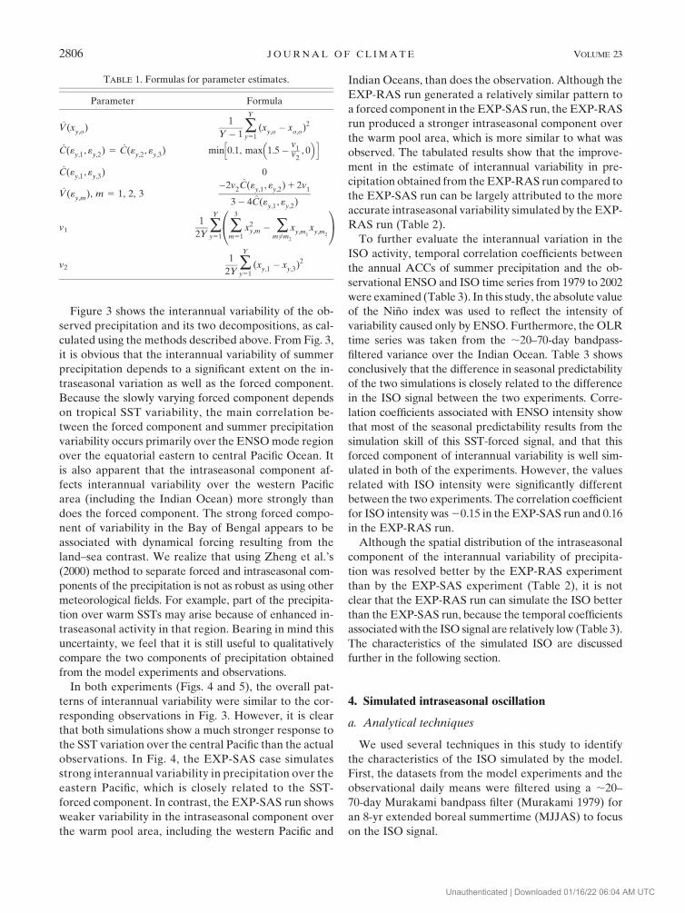
Figure 3 shows the interannual variability of the ob-

served precipitation and its two decompositions, as cal-

culated using the methods described above. From Fig. 3,

it is obvious that the interannual variability of summer

precipitation depends to a significant extent on the in-

traseasonal variation as well as the forced component.

Because the slowly varying forced component depends

on tropical SST variability, the main correlation be-

tween the forced component and summer precipitation

variability occurs primarily over the ENSO mode region

over the equatorial eastern to central Pacific Ocean. It

is also apparent that the intraseasonal component af-

fects interannual variability over the western Pacific

area (including the Indian Ocean) more strongly than

does the forced component. The strong forced compo-

nent of variability in the Bay of Bengal appears to be

associated with dynamical forcing resulting from the

land–sea contrast. We realize that using Zheng et al.’s

(2000) method to separate forced and intraseasonal com-

ponents of the precipitation is not as robust as using other

meteorological fields. For example, part of the precipita-

tion over warm SSTs may arise because of enhanced in-

traseasonal activity in that region. Bearing in mind this

uncertainty, we feel that it is still useful to qualitatively

compare the two components of precipitation obtained

from the model experiments and observations.

In both experiments (Figs. 4 and 5), the overall pat-

terns of interannual variability were similar to the cor-

responding observations in Fig. 3. However, it is clear

that both simulations show a much stronger response to

the SST variation over the central Pacific than the actual

observations. In Fig. 4, the EXP-SAS case simulates

strong interannual variability in precipitation over the

eastern Pacific, which is closely related to the SST-

forced component. In contrast, the EXP-SAS run shows

weaker variability in the intraseasonal component over

the warm pool area, including the western Pacific and

Indian Oceans, than does the observation. Although the

EXP-RAS run generated a relatively similar pattern to

a forced component in the EXP-SAS run, the EXP-RAS

run produced a stronger intraseasonal component over

the warm pool area, which is more similar to what was

observed. The tabulated results show that the improve-

ment in the estimate of interannual variability in pre-

cipitation obtained from the EXP-RAS run compared to

the EXP-SAS run can be largely attributed to the more

accurate intraseasonal variability simulated by the EXP-

RAS run (Table 2).

To further evaluate the interannual variation in the

ISO activity, temporal correlation coefficients between

the annual ACCs of summer precipitation and the ob-

servational ENSO and ISO time series from 1979 to 2002

were examined (Table 3). In this study, the absolute value

of the Nino index was used to reflect the intensity of

variability caused only by ENSO. Furthermore, the OLR

time series was taken from the ;20–70-day bandpass-

filtered variance over the Indian Ocean. Table 3 shows

conclusively that the difference in seasonal predictability

of the two simulations is closely related to the difference

in the ISO signal between the two experiments. Corre-

lation coefficients associated with ENSO intensity show

that most of the seasonal predictability results from the

simulation skill of this SST-forced signal, and that this

forced component of interannual variability is well sim-

ulated in both of the experiments. However, the values

related with ISO intensity were significantly different

between the two experiments. The correlation coefficient

for ISO intensity was 20.15 in the EXP-SAS run and 0.16

in the EXP-RAS run.

Although the spatial distribution of the intraseasonal

component of the interannual variability of precipita-

tion was resolved better by the EXP-RAS experiment

than by the EXP-SAS experiment (Table 2), it is not

clear that the EXP-RAS run can simulate the ISO better

than the EXP-SAS run, because the temporal coefficients

associated with the ISO signal are relatively low (Table 3).

The characteristics of the simulated ISO are discussed

further in the following section.

4. Simulated intraseasonal oscillation

a. Analytical techniques

We used several techniques in this study to identify

the characteristics of the ISO simulated by the model.

First, the datasets from the model experiments and the

observational daily means were filtered using a ;20–

70-day Murakami bandpass filter (Murakami 1979) for

an 8-yr extended boreal summertime (MJJAS) to focus

on the ISO signal.

TABLE 1. Formulas for parameter estimates.

Parameter Formula

V(xy,o)1

Y � 1�Y

y51(xy,o � xo,o)2

C(«y,1, «y,2) 5 C(«y,2, «y,3) min 0.1, max 1.5� v1v2

, 0� �h i

C(«y,1, «y,3) 0

V(«y,m

), m 5 1, 2, 3�2v2C(«y,1, «y,2) 1 2v1

3� 4C(«y,1

, «y,2

)

v1

1

2Y�Y

y51�

3

m51x2

y,m � �m 6¼m2

xy,m1

xy,m2

0@

1A

v2

1

2Y�Y

y51(xy,1 � xy,3)2



FIG. 3. Global distributions of observed summer mean precipitation (mm day21) re-

constructed by the method of Zheng et al. (2000): (a) interannual variability of CMAP,

(b) variability resulting from the forced component, and (c) variability resulting from the

intraseasonal component.

15 MAY 2010 P A R K E T A L . 2807


FIG. 4. As in Fig. 3, but for the EXP-SAS run.



FIG. 5. As in Fig. 3, but for the EXP-RAS run.

15 MAY 2010 P A R K E T A L . 2809


In addition, a space–time spectral analysis was per-

formed to capture the characteristics of propagating

waves. This technique is useful for analyzing zonally

propagating waves, because it decomposes the time and

longitude-dependent data stream into wavenumber and

frequency components for eastward- and westward-

propagating waves as well as zonal-mean fluctuations

(Hayashi 1982). To prevent aliasing, a spectral analysis

was applied to the seasonal cycle–removed daily anom-

alies. The seasonal cycle for each particular year was

defined as the sum of the first two harmonics at each grid

point. After the seasonal cycles were removed, the mean

and linear trends of each segment were removed in time

by a least squares fit, and then the ends of the series were

tapered to zeros. Further, to reduce noise, the space–time

spectra were generated for 8 yr by applying a 30-day

overlap to successive 92-day data segments, as in Wheeler

and Kiladis (1999).

Although ordinary empirical orthogonal function

(EOF) analysis can determine stationary variability, it is

not appropriate for studying the ISO because EOF is

only applicable to stationary waves. We therefore ap-

plied complex empirical orthogonal function (CEOF)

analysis (Horel 1984; Yih and Kwon 2006) to the ;20–

70-day velocity potential fields to determine the domi-

nant propagating mode embedded in the datasets.

b. Comparison of the simulated ISO

The global distributions of the approximately 20–70-day

precipitation variance from the observations and sim-

ulations are compared in Fig. 6. Overall, the EXP-SAS

and EXP-RAS experiments showed similar patterns in

terms of dominant variance over the Indian Ocean and

the western Pacific region, compared to those from the

GPCP observation. However, the magnitude simulated

by both experimental runs was larger than the obser-

vation over these regions. Further, it is clear that the

EXP-SAS experiment exaggerates the variance along the

ITCZ over the central and eastern Pacific and the South

Pacific convergence zone (SPCZ) over the western Pacific.

The variance from the EXP-RAS run is closer to that

observed along the ITCZ and SPCZ; however, it is ob-

vious that the EXP-RAS run shows exaggerated vari-

ance over a broader region, from the Indian Ocean to

the western Pacific. The distribution of the approximately

20–70-day precipitation variance in Fig. 6 resembles the

seasonal precipitation in Fig. 1, indicating that the ISO

signals analyzed in this section comply with the signals in

the SMIP runs discussed in the previous section. Indeed,

the overall distribution of the 8-yr-averaged JJA pre-

cipitation was found to be close to what was shown in

Fig. 1 (data not shown).

The wave characteristics of the simulated ISO were

compared to those from the GPI observations in Fig. 7,

after applying wavenumber–frequency spectral analysis

to equatorial precipitation. In Fig. 7a, it is clear that the

dominant mode in the observations is the eastward-

propagating wave with a 46-day period and a wavenumber

of 1. This observational feature of ISO is consistent with

the results of many previous analyses that used outgoing

longwave radiation (OLR; e.g., Wheeler and Kiladis

1999) and precipitation (e.g., Zhang and Mu 2005; Lin

et al. 2006). In contrast, the EXP-SAS simulation (Fig. 7b)

generated a mainly stationary wave of zonal wave-

number 0, and its spectral peak occurred after a period

of 46 days. The dominant propagating mode for wave-

number 1 was the eastward-propagating wave with a

nearly 30-day period. In addition, the EXP-SAS run

showed a westward-propagating wave with a spectral

peak of a ;20–30-day period at wavenumber 4, which is

too strong, but may reflect an observed Rossby wave

frequency. The EXP-RAS case (Fig. 7c) generated a

stationary wave with a 46-day period, similar to the EXP-

SAS run, but its spectral power was larger at the peak than

that of the EXP-SAS experiment, with a longer period.

The dominant eastward-propagating mode simulated by

the EXP-RAS experiment was 1–2, with a 46-day period.

Westward-propagating waves were also generated in the

EXP-RAS run, with the wavenumber ranging between

2 and 4 and a period of approximately 20–30 days.

However, Jiang et al. (2004) reported that the

ISO in the boreal summertime has a significant

TABLE 2. Correlation coefficients for variance decomposition of

the simulated precipitation.

Experiments

Interannual

variability

Forced

component

Intraseasonal

component

EXP-SAS 0.77 0.69 0.76

EXP-RAS 0.81 0.70 0.82

TABLE 3. Temporal correlation coefficients between the annual

ACCs of summer precipitation and the observational ENSO and

ISO time series from 1979 to 2002. The coefficients from the two

simulations for the ENSO and ISO intensities are temporal corre-

lations calculated from the annual ACCs and a time series of ab-

solute values of the Nino-3.4 index, and the variance of ;20–70-day

bandpass-filtered OLR averaged over the Indian Ocean (approxi-

mately 58S–58N, approximately 708–808E), respectively. When these

values were different, the temporal correlation was calculated from

the time series of differences in the annual ACCs predicted by the

two experiments. Values with one or two asterisks indicate co-

efficients significant at the 99% or 90% levels, respectively.

Experiment ENSO intensity ISO intensity

EXP-SAS 0.70* 20.15

EXP-RAS 0.71** 0.16

Difference (RAS 2 SAS) 0.06 0.34*



northward-propagating component. Therefore, the me-

ridional wavenumber–frequency spectra for precipitation

over the western Pacific region were calculated to analyze

propagating waves in the south–north direction; the re-

sults are presented in Figs. 7d–f. It is clear that the ob-

served GPI rainfall has a dominant wave component that

is propagated northward at the peak of 46-day period with

a meridional wavenumber of 1. Note that wavenumber 1

in Figs. 7d–f corresponds to the domain of approximately

108S–37.58N. Furthermore, the southward-propagating

component occurred at wavenumber 1 within the same

period, but with a weaker power than the northward

component. It is clear from Fig. 7e that the EXP-SAS case

is similar to the GPI spectra. However, the two propa-

gating modes in the northward and southward directions

tend to have shorter periods than those in the GPCP GPI

data. In the EXP-RAS simulation (Fig. 7f), it was ap-

parent that the dominant northward-propagating wave

FIG. 6. The 20–70-day precipitation variance (mm2 day22) averaged for 8 yr from 1997 to 2004.

(a) GPI observation, (b) the EXP-SAS run, and (c) the EXP-RAS run.

15 MAY 2010 P A R K E T A L . 2811


FIG. 7. Wavenumber–frequency power spectra of average precipitation for the boreal summers from 1997 to 2004.

(left) Zonal wavenumber spectra averaged over approximately 158S–158N for (a) GPI data, (b) the EXP-SAS run,

and (c) the EXP-RAS run are denoted. (right) Meridional wavenumber spectra averaged over ;1008–1508E for

(d) GPI data, (e) the EXP-SAS run, and (f) the EXP-RAS run are also indicated.



occurred at the same wavenumber and period, but its

spectral power was exaggerated. The EXP-RAS experi-

ment, however, did not clearly distinguish the southward-

propagating wave with wavenumber 1 from the northward

waves, in contrast to the EXP-SAS run.

To better visualize the ISO-related wave characteris-

tics in large-scale circulation, CEOF analysis was applied

to the 200-hPa velocity potential fields from NCEP/DOE

Reanalysis 2 data and two model simulations (Fig. 8). The

velocity potential field was chosen for the analysis of

MJO signal because it can represent the global distri-

bution of upper-level divergence-associated convective

activities. The first CEOF extracted from the obser-

vation accounted for 50% of the total approximately

20–70-day variance, whereas the first modes from the

EXP-SAS and EXP-RAS experiments accounted for 34%

and 36% of the total approximately 20–70-day variance,

respectively. The first modes were well separated from

the other modes, satisfying the criteria of North et al.

(1982), even though the percentages from the model

simulations were smaller than observation percentages.

Nevertheless, Fig. 8 clearly demonstrates that the first

CEOF mode of the 200-hPa velocity potential from the

EXP-RAS run is closer to the observation at day 46 as

compared to the approximately 20–30 days in the case of

the EXP-SAS run, which is consistent with the precipi-

tation analysis in Fig. 7.

Composite fields taken from the first CEOF mode were

constructed to investigate the spatial features of the ISO.

In Fig. 9, the composite velocity potential anomalies for

each phase from 08 to 2708 are shown; the whole phase

range corresponds to the period of the dominant modes

shown in each case. At a 08 phase angle (top panel), the

positive anomaly of the 200-hPa velocity potential (con-

vergence area) appears over the entire Pacific Ocean,

with its maximum at the western Pacific. Furthermore,

the divergence region (negative anomaly of the 200-hPa

velocity potential) covers a broad area from the Atlantic

to the Indian Oceans. In the next phase (second panel),

the divergence area has moved to the Indian Ocean,

whereas the convergence area has moved to the eastern

Pacific. It is clear that the anomaly fields in phase angle

1808 (third panel) show a pattern opposite to that of phase

angle 08 (top panel); similarly, phase angle 2708 (bottom

panel) is the reverse of phase angle 908 (second panel).

The composite velocity potential anomalies from the

two experiments captures the global propagation of the

ISO as atmospheric responses to convective perturba-

tions well; this global propagation is characterized by a

convectively forced Kelvin–Rossby wave moving east-

ward from the western Indian Ocean to the western Pa-

cific with a slow phase speed of about 5 m s21, and a fast

dry Kelvin wave moving from the central Pacific to the

eastern Pacific with a fast phase speed of about 30 m s21

(e.g., Madden and Julian 1972; Salby and Hendon 1994;

Weickmann et al. 1997; Matthews 2000). However, al-

though both experiments agreed qualitatively with the

observations, the two simulations showed faster move-

ment of the convection core (negative anomalies) from

phase angle 908 to 1808 than what was observed. A close

inspection revealed that results from the EXP-RAS were

more realistic in terms of maximum amplitudes and their

locations at each phase than the EXP-SAS run. For ex-

ample, the amplitude of the negative velocity potential

anomaly from the EXP-RAS run was strongest at phase

angle 908, which is consistent with the observed data, but

this negative velocity potential anomaly appeared only in

the next phase in the EXP-SAS run.

5. Summary and concluding remarks

We examined the simulated boreal summer climate

from 1979 to 2002 using a GCM with two different con-

vective parameterization schemes—the SAS and RAS

algorithms—on a SMIP-type integration test bed. The

characteristics of wave propagation and intensity of the

ISO simulated in extended boreal summers from 1997 to

2004 by the model with two convection schemes were

investigated. The possible link between ISO simulation

and dynamical seasonal prediction was also discussed.

The simulated global precipitation climatology and

interannual variability show that both experiments cap-

ture the global precipitation climatology, and interannual

variability fairly well, but RAS outperforms SAS in terms

of bias, root-mean-square error, and anomaly correlation

coefficients. Decomposition of the interannual variability

of summer precipitation into two components indicated

FIG. 8. Power spectra for time series of the first CEOF mode of

the 200-hPa velocity potential. The NCEP/DOE Reanalysis 2 data

(solid lines), and the EXP-SAS (dotted lines) and the EXP-RAS

(dashed lines) experiments are denoted.

15 MAY 2010 P A R K E T A L . 2813


that the observed interannual variability of the summer

mean precipitation is dominated by the intraseasonal

component over the warm pool area and the SST-forced

signal prevailing over the equatorial Pacific Ocean. The

major difference between the two model simulations is

the interannual variability over the warm pool area,

which is associated with differences in the simulation of

the intraseasonal component. The temporal correlation

coefficients between the annual anomaly correlation co-

efficients of summer precipitation and the observational

ENSO and ISO time series also indicate that most of the

seasonal predictability results from the simulation skill

of the SST-forced signal, and the difference in seasonal

predictability of the two simulations is closely related to

the difference in the ISO signal, although the significance

of this is relatively low.

When we compared the simulated ISO values, we

found that the global distributions of the approximately

20–70-day precipitation variance and the wave character-

istics of the simulated ISO were fairly well reproduced by

the model regardless of the convection scheme. However,

the power spectra for the time series of the first CEOF

FIG. 9. Composite of the 200-hPa velocity potential anomalies (106 m2 s21) taken from (top) the NCEP/DOE Reanalysis 2, (left) the

EXP-SAS run, and (right) EXP-RAS run. Segments are separated by 908, with phase angles increasing from top to bottom.



mode of the 200-hPa velocity potential were closer to

the observed data on day 46 in the RAS run than the

SAS run. The composite fields of the 200-hPa velocity

potential taken from the first CEOF mode revealed that

the global propagation of the ISO as atmospheric re-

sponses to convective perturbations was well reproduced

by both experiments, but the RAS run outperformed the

SAS run in terms of the amplitude of anomalies.

It is not clear from the model results for seasonal

prediction and ISO simulation that accurate ISO simu-

lation guarantees improved seasonal predictability of

boreal summer precipitation, even though some ana-

lyses imply that better ISO simulation can result in better

seasonal prediction. Nevertheless, it is possible to con-

clude that accurate simulation of the ISO is an important

factor toward an improvement of seasonal predictabil-

ity. Traditionally, the predictability of the dynamical

seasonal prediction model has been assessed based on

evaluation of the seasonal mean climate and interannual

variability in the model simulation. However, we have

shown in this study that the seasonal predictability of the

dynamical climate model is also closely related to its

ability to simulate intraseasonal variability accurately. It

is again important to note that the purpose of this re-

search was not to judge the superiority of one algorithm

over another, but to examine the role of intraseasonal

variability in accurate seasonal prediction. For example,

the seasonal mean tropical precipitation simulated by the

SAS run was closer to the actual observations than the

precipitation simulated by the RAS scheme when the re-

vised vertical diffusion scheme was employed (Byun and

Hong 2004), indicating that further improvements in the

physical parameterizations of GCMs are likely to improve

climate prediction.

Acknowledgments. This research was supported by

project NIMR-2009-B-2 of the National Institute of

Meteorological Research in Korea Meteorological Ad-

ministration, and by the Basic Science Research Program

through the National Research Foundation of Korea

(NRF) funded by the Ministry of Education, Science

and Technology (2010-0000840).

REFERENCES

Anderson, J., H. M. Van Den Dool, A. Barnston, W. Chen, W. Stern,

and J. Ploshay, 1999: Present-day capabilities of numerical and

statistical models for atmospheric extratropical seasonal simu-

lation and prediction. Bull. Amer. Meteor. Soc., 80, 1349–1361.

Arakawa, A., and W. H. Schubert, 1974: Interaction of a cumulus

ensemble with the large-scale environment. Part I. J. Atmos.

Sci., 31, 674–704.

Barnston, A. G., S. J. Mason, L. Goddard, D. G. Dewitt, and

S. E. Zebiak, 2003: Multimodel ensembling in seasonal climate

forecasting at IRI. Bull. Amer. Meteor. Soc., 84, 1783–1796.

Byun, Y.-H., and S.-Y. Hong, 2004: Impact of boundary layer

processes on simulated tropical rainfall. J. Climate, 17, 4032–

4044.

——, and ——, 2007: Improvements in the subgrid-scale repre-

sentation of moist convection in a cumulus parameterization

scheme: The single-column test and its impact on seasonal

prediction. Mon. Wea. Rev., 135, 2135–2154.

Donner, L. J., C. J. Seman, R. S. Hemler, and S. Fan, 2001: A

cumulus parameterization including mass fluxes, convective

vertical velocities, and mesoscale effects: Thermodynamic and

hydrological aspects in a general circulation model. J. Climate,

14, 3444–3463.

Goswami, B. N., G. Wu, and T. Yasunari, 2006: The annual cycle,

intraseasonal oscillations, and roadblock to seasonal predict-

ability of the Asian summer monsoon. J. Climate, 19, 5078–5099.

Graham, N. E., and T. P. Barnett, 1995: ENSO and ENSO-related

predictability. Part II: Northern Hemisphere 700-mb height

predictions based on a hybrid coupled ENSO model. J. Cli-

mate, 8, 544–549.

Gregory, D., R. Kershaw, and P. M. Inness, 1997: Parameterization

of momentum transports by convection II: Tests in single

column and general models. Quart. J. Roy. Meteor. Soc., 123,

1153–1183.

Grell, G. A., 1993: Prognostic evaluation of assumptions used by

cumulus parameterization. Mon. Wea. Rev., 121, 764–787.

Hayashi, Y., 1982: Space-time spectral analysis and its applications

to atmospheric waves. J. Meteor. Soc. Japan, 60, 156–171.

Horel, J. D., 1984: Complex principal component analysis: Theory

and examples. J. Climate Appl. Meteor., 23, 1660–1673.

Huffman, G. J., R. F. Adler, M. Morrissey, D. T. Bolvin, S. Curtis,

R. Joyce, B. McGavock, and J. Susskind, 2001: Global pre-

cipitation at one-degree daily resolution from multisatellite

observations. J. Hydrometeor., 2, 36–50.

Jiang, X., T. Li, and B. Wang, 2004: Structures and mechanisms of

the northward propagating boreal summer intraseasonal os-

cillation. J. Climate, 17, 1022–1039.

Jones, C., D. E. Waliser, K. M. Lau, and W. Stern, 2004: The

Madden–Julian oscillation and its impact on Northern Hemi-

sphere weather predictability. Mon. Wea. Rev., 132, 1462–1471.

Kalnay, E., and Coauthors, 1996: The NCEP/NCAR 40-Year Re-

analysis Project. Bull. Amer. Meteor. Soc., 77, 437–471.

Kanamitsu, M., and Coauthors, 2002a: NCEP dynamical seasonal

forecast system 2000. Bull. Amer. Meteor. Soc., 83, 1019–1037.

——, W. Ebisuzaki, J. Woollen, S.-K. Yang, J. J. Hnilo, M. Fiorino,

and G. L. Potter, 2002b: NCEP–DOE AMIP-II Reanalysis

(R-2). Bull. Amer. Meteor. Soc., 83, 1631–1643.

Kang, I.-S., S.-I. An, C.-H. Joung, S.-C. Yoon, and S.-M. Lee, 1989:

30-60 day oscillation appearing in climatological variation of

outgoing longwave radiation around East Asia during sum-

mer. J. Korean Meteor. Soc., 25, 221–232.

——, J.-Y. Lee, and C.-K. Park, 2004: Potential predictability of

summer mean precipitation in a dynamical seasonal prediction

system with systematic error correction. J. Climate, 17, 834–844.

Kim, B.-M., G.-H. Lim, and K.-Y. Kim, 2006: A new look at the

midlatitude–MJO teleconnection in the Northern Hemisphere

winter. Quart. J. Roy. Meteor. Soc., 132, 485–503.

Kumar, A., M. Hoerling, M. Ji, A. Leetmaa, and P. Sardeshmukh,

1996: Assessing a GCM’s suitability for making seasonal pre-

dictions. J. Climate, 9, 115–129.

Lee, M.-I., I.-S. Kang, and B. E. Mapes, 2003: Impacts of cumulus

convection parameterization on aqua-planet AGCM simula-

tions of tropical intraseasonal variability. J. Meteor. Soc. Japan,

81, 963–992.

15 MAY 2010 P A R K E T A L . 2815


Liess, S., D. E. Waliser, and S. D. Schubert, 2005: Predictability

studies of the intraseasonal oscillation with the ECHAM5

GCM. J. Atmos. Sci., 62, 3320–3336.

Lin, J.-L., and Coauthors, 2006: Tropical intraseasonal variability

in 14 IPCC AR4 climate models. Part I: Convective signals.

J. Climate, 19, 2665–2690.

Lorenz, D. J., and D. L. Hartmann, 2006: The effect of the MJO on

the North American monsoon. J. Climate, 19, 333–343.

Madden, R. A., and P. R. Julian, 1972: Description of global-scale

circulation cells in the tropics with a 40–50-day period. J. At-

mos. Sci., 29, 1109–1123.

——, and ——, 1994: Observations of the 40–50-day tropical os-

cillation: A review. Mon. Wea. Rev., 122, 814–837.

Matthews, A. J., 2000: Propagation mechanisms for the Madden-

Julian oscillation. Quart. J. Roy. Meteor. Soc., 126, 2637–2651.

Mo, R., and D. M. Straus, 2002: Statistical–dynamical seasonal

prediction based on principal component regression of GCM

ensemble integrations. Mon. Wea. Rev., 130, 2167–2187.

Moorthi, S., and M. J. Suarez, 1992: Relaxed Arakawa–Schubert: A

parameterization of moist convection for general circulation

models. Mon. Wea. Rev., 120, 978–1002.

Murakami, M., 1979: Large-scale aspects of deep convective activity

over the GATE Area. Mon. Wea. Rev., 107, 994–1013.

Nobre, P., A. D. Moura, and L. Sun, 2001: Dynamical downscaling

of seasonal climate prediction over Nordeste Brazil with

ECHAM3 and NCEP’s regional spectral models at IRI. Bull.

Amer. Meteor. Soc., 82, 2787–2796.

North, G. R., T. L. Bell, R. F. Cahalan, and F. J. Moeng, 1982:

Sampling errors in the estimation of empirical orthogonal

functions. Mon. Wea. Rev., 110, 699–706.

Palmer, T. N., and Coauthors, 2004: Development of a European

Multimodel Ensemble System for Seasonal-to-Interannual

Prediction (DEMETER). Bull. Amer. Meteor. Soc., 85,

853–872.

Pan, H.-L., and W.-S. Wu, 1995: Implementing a mass flux con-

vective parameterization package for the NMC medium-range

forecast model. NMC Office Note 409, 40 pp.

Reynolds, R. W., and T. M. Smith, 1994: Improved global sea surface

temperature analyses using optimum interpolation. J. Climate,

7, 929–948.

Rowell, D. P., 1998: Assessing potential predictability with an

ensemble of multidecadal GCM simulations. J. Climate, 11,

109–120.

Saha, S., and Coauthors, 2006: The NCEP Climate Forecast Sys-

tem. J. Climate, 19, 3483–3517.

Salby, M. L., and H. H. Hendon, 1994: Intraseasonal behavior of

clouds, temperature, and winds in the tropics. J. Atmos. Sci.,

51, 2207–2224.

Shukla, J., and Coauthors, 2000: Dynamical seasonal prediction.

Bull. Amer. Meteor. Soc., 81, 2593–2606.

Sperber, K. R., and D. E. Waliser, 2008: New approaches to un-

derstanding, simulating, and forecasting the Madden–Julian

oscillation. Bull. Amer. Meteor. Soc., 89, 1917–1920.

Stern, W. F., and K. Miyakoda, 1995: Feasibility of seasonal fore-

casts inferred from multiple GCM simulations. J. Climate, 8,

1071–1085.

Sun, L., D. F. Moncunill, H. Li, A. D. Moura, F. Filho, and

S. E. Zebiak, 2006: An operational dynamical downscaling

prediction system for Nordeste Brazil and the 2002–04 real-

time forecast evaluation. J. Climate, 19, 1990–2007.

Wang, W., and M. E. Schlesinger, 1999: The dependence on con-

vection parameterization of the tropical intraseasonal oscil-

lation simulated by the UIUC 11-layer atmospheric GCM.

J. Climate, 12, 1423–1457.

Weickmann, K. M., G. N. Kiladis, and P. D. Sardeshmukh, 1997:

The dynamics of intraseasonal atmospheric angular momen-

tum oscillations. J. Atmos. Sci., 54, 1445–1461.

Wheeler, M., and G. N. Kiladis, 1999: Convectively coupled

equatorial waves: Analysis of clouds and temperature in the

wavenumber–frequency domain. J. Atmos. Sci., 56, 374–399.

Xie, P., and P. A. Arkin, 1997: Global precipitation: A 17-year

monthly analysis based on gauge observations, satellite esti-

mates, and numerical model outputs. Bull. Amer. Meteor. Soc.,

78, 2539–2558.

Yih, H., and W.-T. Kwon, 2006: Global precipitation characteristics

in CMAP-observation and ECHO-G climate model simula-

tion dataset. J. Korean Meteor. Soc., 42, 209–224.

Zhang, G. J., and M. Mu, 2005: Simulation of the Madden–Julian

oscillation in the NCAR CCM3 using a revised Zhang–

McFarlane convection parameterization scheme. J. Climate,

18, 4046–4064.

Zheng, X., and C. S. Frederiksen, 2004: Variability of seasonal-

mean fields arising from intraseasonal variability: Part 1,

Methodology. Climate Dyn., 23, 177–191.

——, H. Nakamura, and J. A. Renwick, 2000: Potential predictability

of seasonal means based on monthly time series of meteoro-

logical variables. J. Climate, 13, 2591–2604.

Zwiers, F. W., 1996: Interannual variability and predictability in an

ensemble of AMIP climate simulations conducted with the

CCC GCM2. Climate Dyn., 12, 825–847.



Documents

Precipitation in Boreal Summer Simulated by a GCM with Two