Network: Comput. Neural Syst.10 (1999) 285–301. Printed in the UK PII: S0954-898X(99)07931-2

Pre-synaptic lateral inhibition provides a better architecturefor self-organizing neural networks

Michael W SpratlingDivision of Informatics, University of Edinburgh, 5 Forrest Hill, Edinburgh EH1 2QL, UK

Received 7 January 1999, in final form 19 August 1999

Abstract. Unsupervised learning is an important ability of the brain and of many artificial neuralnetworks. A large variety of unsupervised learning algorithms have been proposed. This papertakes a different approach in considering the architecture of the neural network rather than thelearning algorithm. It is shown that a self-organizing neural network architecture using pre-synapticlateral inhibition enables a single learning algorithm to find distributed, local, and topologicalrepresentations as appropriate to the structure of the input data received. It is argued that suchan architecture not only has computational advantages but is a better model of cortical self-organization.

1. Introduction

The pattern of activity of the nodes in a neural network constitutes a representation of the inputto that network. In unsupervised learning, unlike supervised learning, what node activationsconstitute a good representation of the current input is not explicitly defined by the training data.Thus many different algorithms have been proposed (Becker and Plumbley 1996, Barlow 1989)which impose various, application-independent, measures of ‘goodness’ on the representationformed—such as information preservation, minimum redundancy, minimum entropy, densityestimation over priors, maximum-likelihood parameter estimation, and topology preservation.Such algorithms may be implemented using local learning rules or via the optimization of anobjective function. By modifying the learning rules and activation function, or by modifyingthe objective function, the same neural network architecture may be used to find representationsthat preserve different measures of ‘goodness’ (e.g. Oja (1995), cf. Foldiak (1990) and Foldiak(1989), cf. Fyfe (1997) and Harpur and Prager (1996), cf. Sirosh and Miikkulainen (1994) andFoldiak (1990)).

In broad terms these algorithms can be classified with respect to the general form ofrepresentation that is learnt. In a distributed code the activity of a population of nodes providesthe representation. Depending on the size of this active population, in relation to the totalnumber of nodes, this may be a dense or sparse code. In the limit a sparse code becomes alocal code in which a single node provides the representation as the only active node (throughhard, or winner-take-all, competition). In addition, the topological structure of the input spacemay be preserved by placing an ordering on the nodes. With a distributed code all the nodes mayrepresent the same feature of the input; however, it is also possible that different nodes representdifferent aspects of the input pattern, or (equivalently) the simultaneous presentation of multipleinputs. Such a code is described as factorial. In contrast, the simultaneous presentation ofmultiple inputs, or the underlying factors of a particular input, can only be represented by a

0954-898X/99/040285+17$30.00 © 1999 IOP Publishing Ltd 285

286 M W Spratling

single node when using a local code, requiring distinct ‘grandmother cells’ to represent eachcombination of inputs.

Within the diversity of unsupervised learning algorithms which have been proposed, allof these forms of representation can be learnt; however, no single algorithm learns them all.Thus, in order to learn a good representation for a particular task the appropriate form ofencoding must be known beforehand in order to select an appropriate algorithm. In addition,an algorithm which finds a specific, predefined, form of representation fails to model thediversity of structure found in the cortex. Cortical representations vary with sparse distributedcoding (Foldiak and Young 1995, Olshausen and Field 1996), possibly, where appropriate,local coding (Thorpe 1995), as well as topological maps (Swindale 1996, Knudsenet al1990)all being used. Since there is evidence to suggest that neurons, from all areas of the neocortex,apply the same learning mechanisms (Sur 1989, O’Leary 1993, Johnson 1997), it would seemto be important to have a single artificial neural network model which can generate all of theseforms of representation. This paper introduces a self-organizing neural network architecturewhich, using a single learning algorithm, can generate distributed, local, and topologicalrepresentations, as appropriate to the structure of the input data received.

2. Models of lateral inhibition

Lateral inhibition is an essential feature of many artificial, self-organizing, neural networks. Itprovides a mechanism through which neurons compete to represent distinct patterns within theinput space. It can be used to decorrelate the activations of nodes, so that the response of thenetwork is a distributed representation of the input (Foldiak 1990). Stronger lateral inhibitioncan be used to generate a local encoding, where a single node inhibits all others (Yuille andGeiger 1995). In addition, by allowing the lateral inhibition strength to vary as a function ofthe distance between nodes it is possible to preserve the topology of the input space (Swindale1996, Sirosh and Miikkulainen 1994).

2.1. The standard model

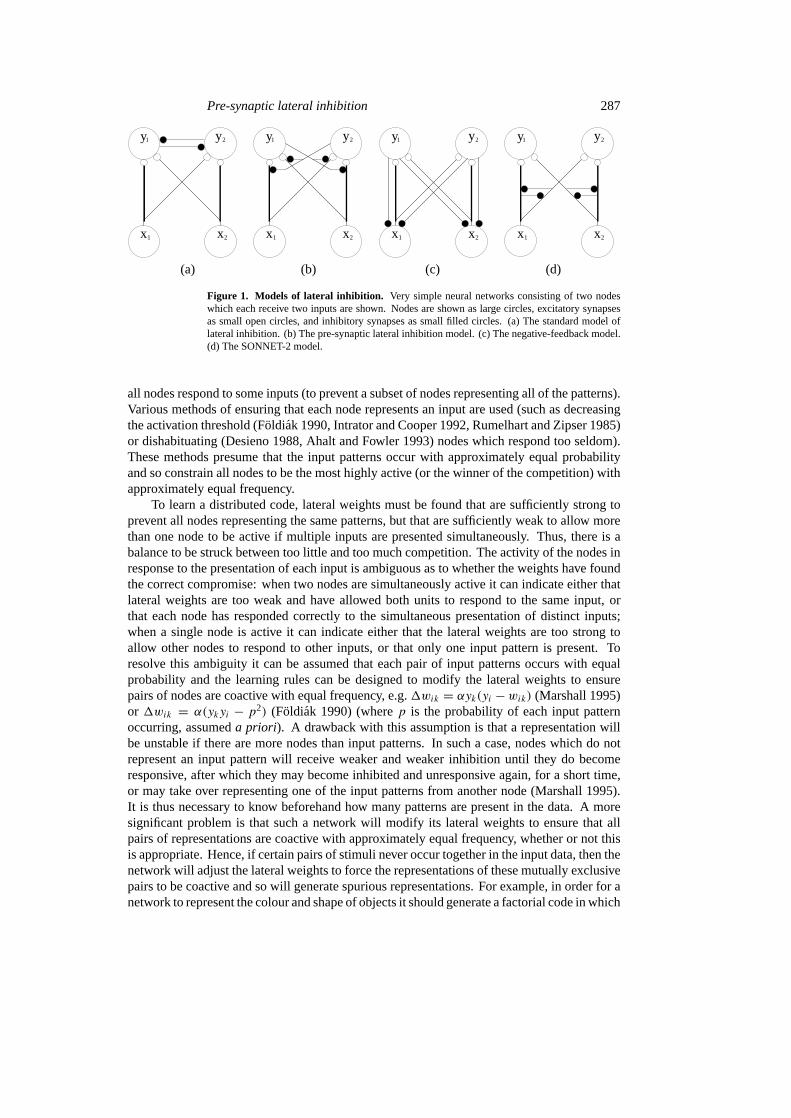
The majority of self-organizing neural networks use lateral inhibition to provide competitionbetween the outputs of nodes (Foldiak 1989, 1990, Marshall 1995, Sirosh and Miikkulainen1994, Swindale 1996), or produce the same effect without explicitly representing connectionsbetween nodes (Kohonen 1997, Ritteret al1992, Rumelhart and Zipser 1985). This ‘standard’architecture (as shown for a simple network of two nodes in figure 1(a)) consists of alayer of neurons each of which receives excitatory inputs (xj ) from a receptive field (RF).The feedforward synaptic weights (qij ) are refined by a learning algorithm to generate arepresentation of the input space. Lateral inhibition, via inhibitory synaptic weights (wik),occurs between the outputs of nodes (yi) to provide competition for the refinement of thefeedforward weights. At equilibrium the output of each node will be

yi =m∑j=1

(qij xj )−n∑

k=1(k 6=i)(wikyk).

This standard architecture has been used (with variations to the learning rules used) tofind distributed, local, and topological representations. However, no single algorithm learnsthem all, due to conflicting requirements for lateral inhibition in forming local and distributedrepresentations.

To learn a local representation the lateral weights simply need to become sufficientlystrong to allow the activity of a single node to be dominant at any one time, while ensuring that

Pre-synaptic lateral inhibition 287

y1 y2 y1 y2

1x x2 1x x2 1x x2

y1 y2 y1 y2

1x x2

(a) (b) (c) (d)

Figure 1. Models of lateral inhibition. Very simple neural networks consisting of two nodeswhich each receive two inputs are shown. Nodes are shown as large circles, excitatory synapsesas small open circles, and inhibitory synapses as small filled circles. (a) The standard model oflateral inhibition. (b) The pre-synaptic lateral inhibition model. (c) The negative-feedback model.(d) The SONNET-2 model.

all nodes respond to some inputs (to prevent a subset of nodes representing all of the patterns).Various methods of ensuring that each node represents an input are used (such as decreasingthe activation threshold (Foldiak 1990, Intrator and Cooper 1992, Rumelhart and Zipser 1985)or dishabituating (Desieno 1988, Ahalt and Fowler 1993) nodes which respond too seldom).These methods presume that the input patterns occur with approximately equal probabilityand so constrain all nodes to be the most highly active (or the winner of the competition) withapproximately equal frequency.

To learn a distributed code, lateral weights must be found that are sufficiently strong toprevent all nodes representing the same patterns, but that are sufficiently weak to allow morethan one node to be active if multiple inputs are presented simultaneously. Thus, there is abalance to be struck between too little and too much competition. The activity of the nodes inresponse to the presentation of each input is ambiguous as to whether the weights have foundthe correct compromise: when two nodes are simultaneously active it can indicate either thatlateral weights are too weak and have allowed both units to respond to the same input, orthat each node has responded correctly to the simultaneous presentation of distinct inputs;when a single node is active it can indicate either that the lateral weights are too strong toallow other nodes to respond to other inputs, or that only one input pattern is present. Toresolve this ambiguity it can be assumed that each pair of input patterns occurs with equalprobability and the learning rules can be designed to modify the lateral weights to ensurepairs of nodes are coactive with equal frequency, e.g.1wik = αyk(yi −wik) (Marshall 1995)or 1wik = α(ykyi − p2) (Foldiak 1990) (wherep is the probability of each input patternoccurring, assumeda priori). A drawback with this assumption is that a representation willbe unstable if there are more nodes than input patterns. In such a case, nodes which do notrepresent an input pattern will receive weaker and weaker inhibition until they do becomeresponsive, after which they may become inhibited and unresponsive again, for a short time,or may take over representing one of the input patterns from another node (Marshall 1995).It is thus necessary to know beforehand how many patterns are present in the data. A moresignificant problem is that such a network will modify its lateral weights to ensure that allpairs of representations are coactive with approximately equal frequency, whether or not thisis appropriate. Hence, if certain pairs of stimuli never occur together in the input data, then thenetwork will adjust the lateral weights to force the representations of these mutually exclusivepairs to be coactive and so will generate spurious representations. For example, in order for anetwork to represent the colour and shape of objects it should generate a factorial code in which

288 M W Spratling

nodes representing different colours and different shapes can be coactive. Using this form oflateral inhibition such a network will correctly respond to white squares and black triangles,but will also generate representations of black–white squares and black square–triangles eventhough such stimuli never exist in the input data. Hence, this form of lateral inhibition fails toprovide factorial coding except for the exceptional case in which all pairs of patterns co-occurtogether. Furthermore, this approach is also incompatible with using lateral inhibition to forma topological representation, since modifying the strength of competition by a function ofthe distance between the nodes would upset the delicate balance in the strength of the lateralweights.

The rules for learning lateral weights to produce local coding and those to producedistributed coding are incompatible. The rules for local coding cannot be used to form afactorial representation since they allow only one node to be active at a time. Alternatively, therules for factorial coding cannot be used to represent mutually exclusive inputs since the lateralweights would weaken until each pair of nodes was occasionally coactive. This incompatibilityis a fundamental limitation of the architecture used, not of any particular learning algorithm.Hence, modification to the architecture rather than the learning rules is required.

2.2. Pre-synaptic lateral inhibition

An architecture that uses lateral inhibition of pre-synaptic inputs (figure 1(b)), to providecompetition for inputs rather than between outputs, overcomes the incompatibility betweenlocal and distributed coding. At equilibrium, the output of each node will be

yi =m∑j=1

(qij xj −

n∑k=1(k 6=i)

(wikj yk)

)+

.

Wherewikj is the strength of the inhibitory synapse from nodek to synapsej of nodei, and(z)+ is the positive half-rectified value ofz.

If the lateral weights have somehow become selective in only inhibiting inputs to which theinhibiting node is most responsive, then each node will attempt to ‘block’ its preferred inputsfrom activating other nodes. If two nodes try to represent the same input pattern, there willbe strong competition between them. If two nodes represent distinct patterns, each node canrespond to its preferred input without inhibiting the other node (assuming that there is not muchoverlap between patterns). Thus the only constraint, for both local and distributed coding, isthat lateral weights are sufficiently strong to allow nodes to claim their preferred input pattern.There is thus no incompatibility between the requirements for local and factorial coding, andan identical algorithm can find either, as appropriate to the input data. In addition, since lateralweights can continue to increase, modifying them by a function of distance between nodes (toencourage the formation of a topologically ordered representation) does not prevent correctcodes being found eventually. Any learning algorithm that refines the lateral weights to allowa node to strongly inhibit its preferred input pattern from reaching other nodes, while reducingits inhibition of other inputs, can generate distributed, local, and topological representations.This ability is primarily a property of the architecture rather than any particular learning rules.Furthermore, since this method only needs to assume that the firing rates of individual nodesare equal, rather than coactivations of pairs of nodes, it is stable if there are more, or less, nodesthan input patterns and if the input data contain pairs of patterns which are mutually exclusive.

One disadvantage of this architecture would seem to be the larger number of lateral weightsrequired; however, these weights do not need to be individually learnt, resulting in this methodbeing computationally efficient. In order for a node,k, to block one of its preferred inputs,j , from activating another node,i, the lateral weightwikj needs to inhibit the inputj from

Pre-synaptic lateral inhibition 289

reaching nodei. This needs to happen if the inhibiting node,k, is responsive to inputj , i.e.wikjneeds to be strong ifqkj is strong. Thus, the lateral weights need simply to be a scaled versionof the inhibiting node’s feedforward weights, i.e.

wikj = α

βqkj

and the activation function becomes

yi =m∑j=1

(qij xj −

n∑k=1(k 6=i)

(α

βqkjyk

))+

.

In a biologically plausible model, the lateral weights could be represented and learnt separately,using a learning rule, such as1wikj = αf lateral(xj , yk)—while the feedforward weights werelearnt, independently, as1qkj = βf forward(yk, xj ). The assumption is simply that the learningrule for the forward weights (f forward) is equivalent to the learning rule for the lateral weights(f lateral), and that both weights have the same initial value.

Further reduction in computational complexity is achieved since the output of the networkcan be found without numerical integration. Instead, the process of competition between thenodes can be approximated by selecting a single winning node (‘win’) to inhibit all of theothers at each iteration:

ywin =m∑j=1

(qwin,j xj )

yi =m∑j=1

(qij xj − α

βqwin,j ywin

)+

∀i 6= win.

The inhibiting node is selected to be that which is most strongly activated by the current input(i.e. the node for which

∑j qij xj is greatest), but modified by a habituation function to keep

all nodes winning with approximately equal probability. This simplification succeeds sincethe inhibiting node competes with all others, forcing preferred inputs to become differentiated.However, since nodes which have learnt distinct input patterns do not inhibit each other, it doesnot, necessarily, generate a local code, and other nodes can continue to respond (and learn)even if they have not been selected as the winner.

The pre-synaptic lateral inhibition architecture was implemented within a competitivelearning algorithm. For each stimulus presented to the network, the node,i, with the highestvalue of (∑

j

qij xj

)(1 +µ(I − nPi)) + ν

was selected to inhibit all others (wherePi is the number of iterations for which nodei wasthe winning node,I is the total number of iterations,µ is the habituation scale factor, andν is a random variable uniformly distributed in the range±0.005 times the maximum nodeactivation). After inhibition by the winning node (using the equation given in the previousparagraph), learning was performed to update the synaptic weights,qij , as a function ofyiandxj for all nodes. The exact form of the learning rule is not important as long as it has theproperties, described above, of increasing the strength of connection between a node and itspreferred stimulus while decreasing the strength of connection to other inputs. It was foundthat variations of normalized Hebbian learning, the outstar rule, and the covariance rule couldall produce similar results to those given in section 3. The actual learning rule used was

1qij = β[m

(xj

x− 1

)/ m∑k=1

∣∣∣∣xkx − 1

∣∣∣∣][n(yiyi − 1

)+/ n∑k=1

(yk

yk− 1

)+]

290 M W Spratling

wherex = τ x+(1−τ)x is the long-term average of the mean past activity for all of the inputs,yi = τyi + (1− τ)yi is the long-term average of the past output activity for nodei, andm andn are the numbers of inputs and nodes in the network. This rule is qualitatively similar to thecovariance rule, except that the post-synaptic term is only allowed to be greater than or equalto zero. Hence, post-synaptic activation exceeding a threshold is required before synapticmodification is enabled. Also, the terms have been rearranged such that weight changes areproportional to the ratio of the current activity to previous activity, rather than the difference.In addition, the pre- and post-synaptic terms are normalized such that the total change insynaptic weight that can occur at each iteration is normalized across the network and forindividual dendrites. This gives equal importance to each training pattern. Synaptic weightswere initialized to have zero strength (tests indicate that random initial weights can also beused). Results were fairly insensitive to the values of the parameters used. All of the resultsshown in this paper were generated using the parametersα = 0.0009,β = 0.000 002 25,τ = 0.001, andµ = 0.001.

2.3. Other non-standard models of lateral inhibition

It is obvious that inhibition could potentially act between several other points in a neuralnetwork, some more of which have been explored in other non-standard architectures.

2.3.1. The negative-feedback model.In this model (figure 1(c)) inhibitory feedback fromeach node inhibits the inputs to the entire network (Fyfe and Baddeley 1995, Fyfe 1997, Charlesand Fyfe 1998, Harpur and Prager 1996). As with pre-synaptic lateral inhibition, these weightscould be learnt, but as a simplification are set to the same values as the corresponding feed-forward weights. However, unlike in the model proposed here, inhibition is to the inputsthemselves and a node cannot entirely inhibit the input to all other nodes (without entirelyinhibiting its own input). Since the inhibitory strength between individual nodes cannot vary,there is no possibility of finding topological representations (without resorting to direct synapticmodifications on neighbouring nodes (Fyfe 1996)).

2.3.2. SONNET-2. In this model (figure 1(d)) inhibition is between the feedforwardconnections (Nigrin 1993, Marshall and Gupta 1998). The change in weight of the inhibitorysynapses, and the strength of inhibition, is a function of both the output activation of theinhibiting node and the input. In theory this architecture could develop local, distributed, andtopological representations, but it is far more complex than the pre-synaptic lateral inhibitionmodel, and no such results have yet appeared.

2.3.3. Yuille’s winner-take-all model.In this models all of the inputs to a node are inhibitedequally and in proportion to the total output from all other nodes in the network (Yuille andGreynacz 1989, Yuille and Geiger 1995). At equilibrium the activation of each node will be

yi =( m∑j=1

qij xj

)exp

(−λ

∑k 6=i

yk

).

This network was explicitly designed to form winner-take-all representations. In order to bemodified to form a distributed code, it would need to find a compromise value for the lateralinhibition strength to allow more than one node to be active simultaneously, and would thussuffer from the same problems as the standard model.

Pre-synaptic lateral inhibition 291

3. Results

A widely used test for factorial coding is the bars data set (Foldiak 1990, Harpur and Prager1996, Fyfe 1997, Charles and Fyfe 1998, Hintonet al1995, Hinton and Ghahramani 1997). Theinput consists of an 8×8 grid on which each for the 16 possible horizontal and vertical bars areactive with probability1

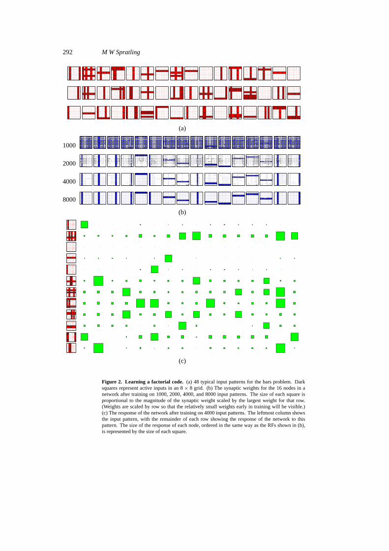
8. Typical examples of input patterns are shown in figure 2(a). When apre-synaptic lateral inhibition network of 16 nodes was trained on these data it found, after 1600presentations, a correct representation, where each node represented exactly one bar and eachbar was represented exactly once. The synaptic weights corresponding to the bar representedbecame much stronger than connections to inputs from other grid points (figure 2(b)) and theresponse of nodes became specific to the presence of that bar in the input data (figure 2(c)).When tested with a further 500 patterns, after training with 4000 pattern presentations, theresponse generated by this network (for input data consisting ofn bars) was such that thenmost active nodes were those which correctly represented all of the active bars in 100% ofunseen (as well as previously seen) test patterns. A more reasonable test is to assume that thenumber of bars in the input pattern is unknown and to analyse only those nodes that have anactivation exceeding a predefined threshold. In this case the active nodes correctly representall of the active bars in the input pattern (and only those bars) for 99% of test patterns. It canbe seen that the greater the number of active bars in a test pattern, the less distinct active nodesbecome with respect to the activity level of other nodes. This is due to the overlap between barsof perpendicular orientation, so an input pattern that contains several bars of one orientationwill partially activate all of the nodes representing bars at the perpendicular orientation.

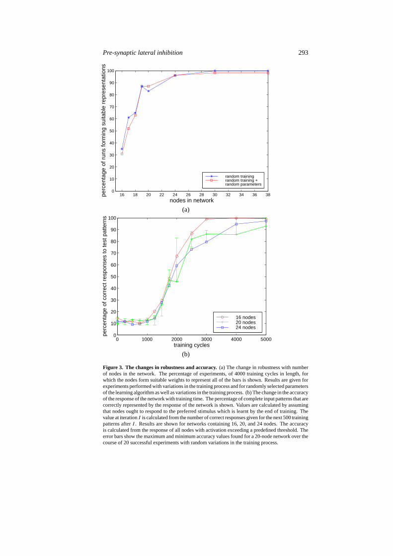
Although the learning algorithm encourages nodes to represent a single unique input,there is no guarantee that this will happen (the results above are for a typical experiment inwhich a suitable encoding was found). The results are sensitive to variations in the trainingprocess (variations caused by different randomly generated training sets), such that with16-node networks one node often came to respond to two separate bars (which were thusindistinguishable to the network) while another node represented none. To test the robustnessof the algorithm, a network consisting of 16 nodes was trained using 54 sets of randomlygenerated training data; of these experiments only 35% learnt to use each node to representa single bar. However, the robustness was improved by using more nodes than there wereindependent input patterns (reaching 100% for a network of 30 nodes; see figure 3(a)). Incases where excess nodes were used, although the allocation of specific bars to specific nodeswas still sensitive to changes in the training process, the algorithm robustly found a subset of 16nodes each of which represented a single unique bar. The robustness of the network to changesin the parameters of the learning algorithm was also tested. Networks consisting of 16 nodestrained using 54 sets of random parameters (with values uniformly chosen in the range±50%from the hand-picked values used above) learnt a suitable representation in only 31% of cases,while networks consisting of more nodes, tested in the same manner, had increasing robustness(see figure 3(a)). These results are extremely similar to the effects of modifying the trainingprocess. Since randomizing the network parameters also resulted in random modificationsto the training process, this suggests that the network is much less sensitive to changes inparameter values than to changes in the learning process.

For a network consisting of 20 nodes (trained using the standard parameter values), thesolution was found within 1200 presentations (see figure 4). When tested with a further 500patterns, after training with 4000 pattern presentations, the response generated by this network(for input data consisting ofn bars) was such that then most active nodes were those whichcorrectly represented all of the active bars in 82% of unseen test patterns. Then most activenodes correctly responded to 94% of all bars presented within those test patterns. Nodes which

292 M W Spratling

(a)

1000

2000

4000

8000

(b)

(c)

Figure 2. Learning a factorial code. (a) 48 typical input patterns for the bars problem. Darksquares represent active inputs in an 8× 8 grid. (b) The synaptic weights for the 16 nodes in anetwork after training on 1000, 2000, 4000, and 8000 input patterns. The size of each square isproportional to the magnitude of the synaptic weight scaled by the largest weight for that row.(Weights are scaled by row so that the relatively small weights early in training will be visible.)(c) The response of the network after training on 4000 input patterns. The leftmost column showsthe input pattern, with the remainder of each row showing the response of the network to thispattern. The size of the response of each node, ordered in the same way as the RFs shown in (b),is represented by the size of each square.

Pre-synaptic lateral inhibition 293

16 18 20 22 24 26 28 30 32 34 36 380

10

20

30

40

50

60

70

80

90

100

nodes in network

perc

enta

ge o

f run

s fo

rmin

g su

itabl

e re

pres

enta

tions

random trainingrandom training +random parameters

(a)

0 1000 2000 3000 4000 50000

10

20

30

40

50

60

70

80

90

100

training cycles

perc

enta

ge o

f cor

rect

res

pons

es to

test

pat

tern

s

16 nodes20 nodes24 nodes

(b)

Figure 3. The changes in robustness and accuracy.(a) The change in robustness with numberof nodes in the network. The percentage of experiments, of 4000 training cycles in length, forwhich the nodes form suitable weights to represent all of the bars is shown. Results are given forexperiments performed with variations in the training process and for randomly selected parametersof the learning algorithm as well as variations in the training process. (b) The change in the accuracyof the response of the network with training time. The percentage of complete input patterns that arecorrectly represented by the response of the network is shown. Values are calculated by assumingthat nodes ought to respond to the preferred stimulus which is learnt by the end of training. Thevalue at iterationI is calculated from the number of correct responses given for the next 500 trainingpatterns afterI . Results are shown for networks containing 16, 20, and 24 nodes. The accuracyis calculated from the response of all nodes with activation exceeding a predefined threshold. Theerror bars show the maximum and minimum accuracy values found for a 20-node network over thecourse of 20 successful experiments with random variations in the training process.

294 M W Spratling

1000

2000

4000

8000

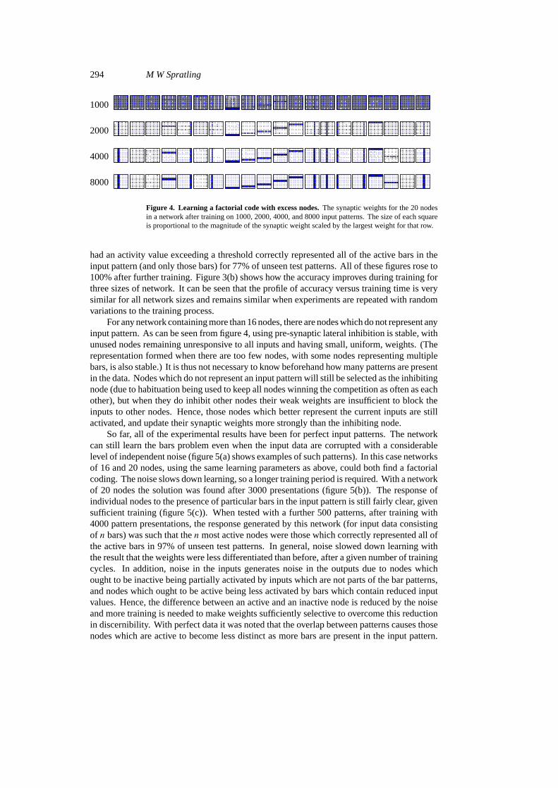
Figure 4. Learning a factorial code with excess nodes.The synaptic weights for the 20 nodesin a network after training on 1000, 2000, 4000, and 8000 input patterns. The size of each squareis proportional to the magnitude of the synaptic weight scaled by the largest weight for that row.

had an activity value exceeding a threshold correctly represented all of the active bars in theinput pattern (and only those bars) for 77% of unseen test patterns. All of these figures rose to100% after further training. Figure 3(b) shows how the accuracy improves during training forthree sizes of network. It can be seen that the profile of accuracy versus training time is verysimilar for all network sizes and remains similar when experiments are repeated with randomvariations to the training process.

For any network containing more than 16 nodes, there are nodes which do not represent anyinput pattern. As can be seen from figure 4, using pre-synaptic lateral inhibition is stable, withunused nodes remaining unresponsive to all inputs and having small, uniform, weights. (Therepresentation formed when there are too few nodes, with some nodes representing multiplebars, is also stable.) It is thus not necessary to know beforehand how many patterns are presentin the data. Nodes which do not represent an input pattern will still be selected as the inhibitingnode (due to habituation being used to keep all nodes winning the competition as often as eachother), but when they do inhibit other nodes their weak weights are insufficient to block theinputs to other nodes. Hence, those nodes which better represent the current inputs are stillactivated, and update their synaptic weights more strongly than the inhibiting node.

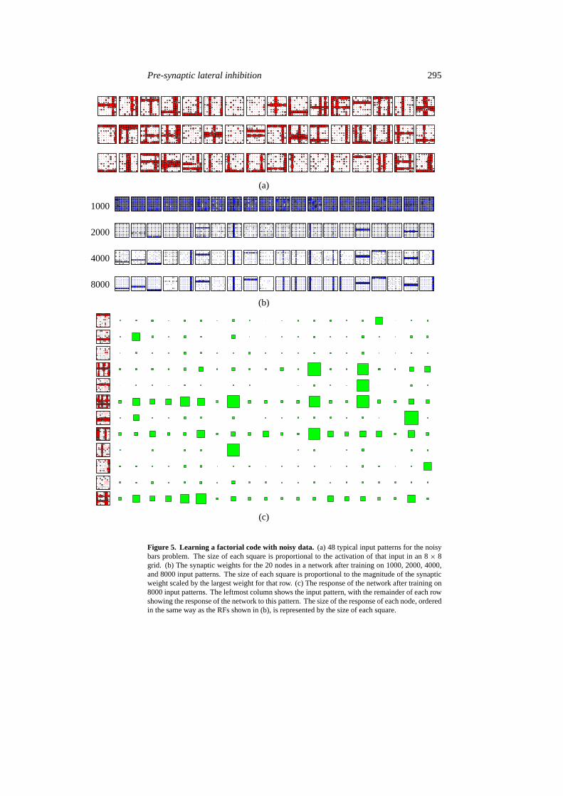
So far, all of the experimental results have been for perfect input patterns. The networkcan still learn the bars problem even when the input data are corrupted with a considerablelevel of independent noise (figure 5(a) shows examples of such patterns). In this case networksof 16 and 20 nodes, using the same learning parameters as above, could both find a factorialcoding. The noise slows down learning, so a longer training period is required. With a networkof 20 nodes the solution was found after 3000 presentations (figure 5(b)). The response ofindividual nodes to the presence of particular bars in the input pattern is still fairly clear, givensufficient training (figure 5(c)). When tested with a further 500 patterns, after training with4000 pattern presentations, the response generated by this network (for input data consistingof n bars) was such that thenmost active nodes were those which correctly represented all ofthe active bars in 97% of unseen test patterns. In general, noise slowed down learning withthe result that the weights were less differentiated than before, after a given number of trainingcycles. In addition, noise in the inputs generates noise in the outputs due to nodes whichought to be inactive being partially activated by inputs which are not parts of the bar patterns,and nodes which ought to be active being less activated by bars which contain reduced inputvalues. Hence, the difference between an active and an inactive node is reduced by the noiseand more training is needed to make weights sufficiently selective to overcome this reductionin discernibility. With perfect data it was noted that the overlap between patterns causes thosenodes which are active to become less distinct as more bars are present in the input pattern.

Pre-synaptic lateral inhibition 295

(a)

1000

2000

4000

8000

(b)

(c)

Figure 5. Learning a factorial code with noisy data. (a) 48 typical input patterns for the noisybars problem. The size of each square is proportional to the activation of that input in an 8× 8grid. (b) The synaptic weights for the 20 nodes in a network after training on 1000, 2000, 4000,and 8000 input patterns. The size of each square is proportional to the magnitude of the synapticweight scaled by the largest weight for that row. (c) The response of the network after training on8000 input patterns. The leftmost column shows the input pattern, with the remainder of each rowshowing the response of the network to this pattern. The size of the response of each node, orderedin the same way as the RFs shown in (b), is represented by the size of each square.

296 M W Spratling

1000

2000

4000

8000

(a)

(b)

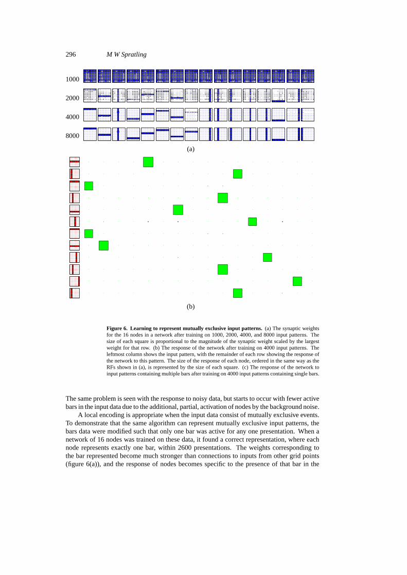
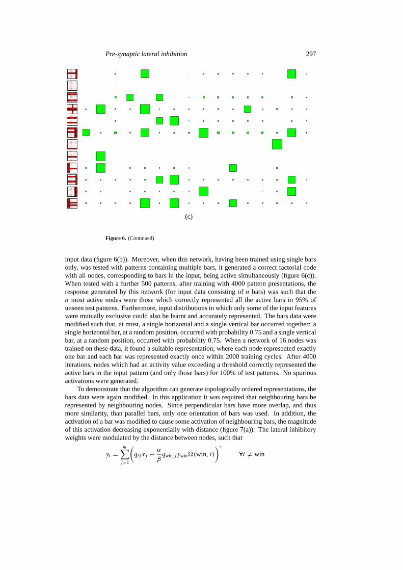
Figure 6. Learning to represent mutually exclusive input patterns. (a) The synaptic weightsfor the 16 nodes in a network after training on 1000, 2000, 4000, and 8000 input patterns. Thesize of each square is proportional to the magnitude of the synaptic weight scaled by the largestweight for that row. (b) The response of the network after training on 4000 input patterns. Theleftmost column shows the input pattern, with the remainder of each row showing the response ofthe network to this pattern. The size of the response of each node, ordered in the same way as theRFs shown in (a), is represented by the size of each square. (c) The response of the network toinput patterns containing multiple bars after training on 4000 input patterns containing single bars.

The same problem is seen with the response to noisy data, but starts to occur with fewer activebars in the input data due to the additional, partial, activation of nodes by the background noise.

A local encoding is appropriate when the input data consist of mutually exclusive events.To demonstrate that the same algorithm can represent mutually exclusive input patterns, thebars data were modified such that only one bar was active for any one presentation. When anetwork of 16 nodes was trained on these data, it found a correct representation, where eachnode represents exactly one bar, within 2600 presentations. The weights corresponding tothe bar represented become much stronger than connections to inputs from other grid points(figure 6(a)), and the response of nodes becomes specific to the presence of that bar in the

Pre-synaptic lateral inhibition 297

(c)

Figure 6. (Continued)

input data (figure 6(b)). Moreover, when this network, having been trained using single barsonly, was tested with patterns containing multiple bars, it generated a correct factorial codewith all nodes, corresponding to bars in the input, being active simultaneously (figure 6(c)).When tested with a further 500 patterns, after training with 4000 pattern presentations, theresponse generated by this network (for input data consisting ofn bars) was such that then most active nodes were those which correctly represented all the active bars in 95% ofunseen test patterns. Furthermore, input distributions in which only some of the input featureswere mutually exclusive could also be learnt and accurately represented. The bars data weremodified such that, at most, a single horizontal and a single vertical bar occurred together: asingle horizontal bar, at a random position, occurred with probability 0.75 and a single verticalbar, at a random position, occurred with probability 0.75. When a network of 16 nodes wastrained on these data, it found a suitable representation, where each node represented exactlyone bar and each bar was represented exactly once within 2000 training cycles. After 4000iterations, nodes which had an activity value exceeding a threshold correctly represented theactive bars in the input pattern (and only those bars) for 100% of test patterns. No spuriousactivations were generated.

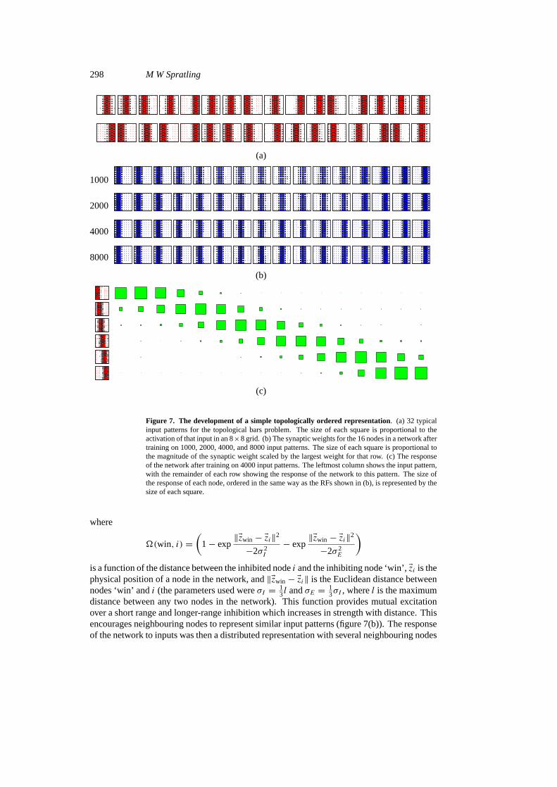
To demonstrate that the algorithm can generate topologically ordered representations, thebars data were again modified. In this application it was required that neighbouring bars berepresented by neighbouring nodes. Since perpendicular bars have more overlap, and thusmore similarity, than parallel bars, only one orientation of bars was used. In addition, theactivation of a bar was modified to cause some activation of neighbouring bars, the magnitudeof this activation decreasing exponentially with distance (figure 7(a)). The lateral inhibitoryweights were modulated by the distance between nodes, such that

yi =m∑j=1

(qij xj − α

βqwin,j ywin�(win, i)

)+

∀i 6= win

298 M W Spratling

(a)

1000

2000

4000

8000

(b)

(c)

Figure 7. The development of a simple topologically ordered representation. (a) 32 typicalinput patterns for the topological bars problem. The size of each square is proportional to theactivation of that input in an 8×8 grid. (b) The synaptic weights for the 16 nodes in a network aftertraining on 1000, 2000, 4000, and 8000 input patterns. The size of each square is proportional tothe magnitude of the synaptic weight scaled by the largest weight for that row. (c) The responseof the network after training on 4000 input patterns. The leftmost column shows the input pattern,with the remainder of each row showing the response of the network to this pattern. The size ofthe response of each node, ordered in the same way as the RFs shown in (b), is represented by thesize of each square.

where

�(win, i) =(

1− exp‖Ezwin − Ezi‖2−2σ 2

I

− exp‖Ezwin − Ezi‖2−2σ 2

E

)is a function of the distance between the inhibited nodei and the inhibiting node ‘win’,Ezi is thephysical position of a node in the network, and‖Ezwin − Ezi‖ is the Euclidean distance betweennodes ‘win’ andi (the parameters used wereσI = 1

3l andσE = 13σI , wherel is the maximum

distance between any two nodes in the network). This function provides mutual excitationover a short range and longer-range inhibition which increases in strength with distance. Thisencourages neighbouring nodes to represent similar input patterns (figure 7(b)). The responseof the network to inputs was then a distributed representation with several neighbouring nodes

Pre-synaptic lateral inhibition 299

0 0.2 0.4 0.6 0.8 10

0.1

0.2

0.3

0.4

0.5

0.6

0.7

0.8

0.9

1

0 0.2 0.4 0.6 0.8 10

0.1

0.2

0.3

0.4

0.5

0.6

0.7

0.8

0.9

1

0 0.2 0.4 0.6 0.8 10

0.1

0.2

0.3

0.4

0.5

0.6

0.7

0.8

0.9

1

0 0.2 0.4 0.6 0.8 10

0.1

0.2

0.3

0.4

0.5

0.6

0.7

0.8

0.9

1

Figure 8. The development of a simple topological map. The map is trained with data uniformlydistributed over the unit square of the two-dimensional plane and is shown (from top to bottom)after training with 1000, 2000, 4000, and 8000 input patterns. Nodes were arranged on a 10-by-10square lattice. Each node is shown projected onto the input plane at the position of its preferredinput, with neighbouring nodes joined by lines.

300 M W Spratling

responding to each input (figure 7(c)). As a more convincing, yet still simple, example oftopological map formation, the same algorithm was applied to the problem of using 100 nodesarranged on a 10-by-10 square lattice to represent points uniformly distributed over the unitsquare of the two-dimensional plane. Figure 8 shows the preferred input of each node, withthose of neighbouring nodes linked by lines.

4. Conclusions

This paper has introduced a neural network architecture that uses pre-synaptic lateral inhibition.The functioning of such a network has been illustrated on some simple test cases. Thispaper suggests that a neural network architecture using pre-synaptic lateral inhibition hassignificant advantages over the standard model of lateral inhibition between node outputs.In this architecture, nodes compete for the right to receive inputs rather than for the rightto generate outputs. Unlike the standard model, this architecture allows a single learningalgorithm to find distributed, local, and (with minor modification) topological representationsof the input. It is thus not necessary to knowa priori the structure of the set of data in orderto generate a good representation for it. In addition, the representations are stable, so it isalso not necessary to knowa priori the number of nodes required to form the representation.Furthermore, these advantages are achieved with no increase in computational complexity overthe standard architecture. These abilities are a function of the network architecture, rather thanany clever learning rules.

The proposed architecture requires inhibition specific to particular synaptic inputs. Suchsynapse-specific inhibition might be implemented biologically either through pre-synapticinhibition via an excitatory synapse on the axon terminal of the excitatory input (Bousher1970, Shepherd 1990, Kandelet al 1995), or through an inhibitory synapse proximal to theexcitatory input on the dendritic tree (Somogyi and Martin 1985). The former mechanismenables an excitatory neuron to directly inhibit the input to another node without the action ofan inhibitory interneuron. However, although, axo-axonal, terminal-to-terminal, synapses arecommon in both vertebrate and invertebrate nervous systems (Brown 1991, Kandelet al1995),there is no evidence for this mechanism of inhibition between cells in the cortex (Mountcastle1998). The latter mechanism relies, as does the standard architecture of lateral inhibition, onthe action of inhibitory interneurons. However, there is also no support for this mechanism ofinhibition in the cortex, since the majority of inhibitory synapses to pyramidal cells terminateon the soma or the axon initial segment rather than the dendrites. Hence, although thisarchitecture is computationally attractive and provides a good model of cortical representation,its implementation is biologically implausible.

References

Ahalt S C and Fowler J E 1993 Vector quantization using artificial neural network modelsProc. Int. Workshop onAdaptive Methods and Emergent Techniques for Signal Processing and Communicationsed D Docampo andA R Figueras, pp 42–61

Barlow H B 1989 Unsupervised learningNeural Comput.1 295–311Becker S and Plumbley M 1996 Unsupervised neural network learning procedures for feature extraction and

classificationInt. J. Appl. Intell.6 185–203Bousher D 1970Introduction to the Anatomy and Physiology of the Nervous System(Oxford: Blackwell)Brown A G 1991Nerve Cells and Nervous Systems: an Introduction to Neuroscience(Berlin: Springer)Charles D and Fyfe C 1998 Modelling multiple cause structure using rectification constraintsNetwork9 167–82Desieno D 1988 Adding a conscience to competitive learningInt. Conf. on Neural Networks(New York: IEEE)

pp 117–24

Pre-synaptic lateral inhibition 301

Foldiak P 1989 Adaptive network for optimal linear feature extractionInt. Joint Conf. on Neural Networks(New York:IEEE) pp 401–5

——1990 Forming sparse representations by local anti-Hebbian learningBiol. Cybernet.64165–70Foldiak P and Young M P 1995 Sparse coding in the primate cortexThe Handbook of Brain Theory and Neural

Networksed M A Arbib (Cambridge, MA: MIT Press) pp 895–8Fyfe C 1996 A scale-invariant feature mapNetwork7 269–75——1997 A neural net for PCA and beyondNeural Process. Lett.6 33–41Fyfe C and Baddeley R 1995 Finding compact and sparse-distributed representations of visual imagesNetwork6

333–44Harpur G and Prager R 1996 Development of low entropy coding in a recurrent networkNetwork7 277–84Hinton G E, Dayan P, Frey B J and Neal R M 1995 The wake–sleep algorithm for unsupervised neural networks

Science2681158–61Hinton G E and Ghahramani Z 1997 Generative models for discovering sparse distributed representationsPhil. Trans.

R. Soc.B 3521177–90Intrator N and Cooper L N 1992 Objective function formulation of the BCM theory of visual cortical plasticity:

statistical connections, stability conditionsNeural Networks5 3–17Johnson M H 1997Developmental Cognitive Neuroscience: an Introduction(Oxford: Blackwell)Kandel E R, Schwartz J H and Jessell T M 1995Essentials of Neural Science and Behavior(Norwalk, CT: Appleton

and Lange)Knudsen E I, du Lac S and Esterly S D 1990 Computational maps in the brainNeurocomputing 2ed J A Anderson

et al (Cambridge, MA: MIT Press) ch 22Kohonen T 1997Self-Organizing Maps(Berlin: Springer)Marshall J A 1995 Adaptive perceptual pattern recognition by self-organizing neural networks: context, uncertainty,

multiplicity, and scaleNeural Networks8 335–62Marshall J A and Gupta V S 1998 Generalization and exclusive allocation of credit in unsupervised category learning

Network9 279–302Mountcastle V B 1998Perceptual Neuroscience: the Cerebral Cortex(Cambridge, MA: Harvard University Press)Nigrin A 1993Neural Networks for Pattern Recognition(Cambridge, MA: MIT Press)Oja E 1995 PCA, ICA, and nonlinear Hebbian learningProc. Int. Conf. on Artificial Neural Networks(London: IEE)

pp 89–94O’Leary D D M 1993 Do cortical areas emerge from a protocortex?Brain Development and Cognition: a Reader

ed M H Johnson (Oxford: Blackwell) pp 323–37Olshausen B A and Field D J 1996 Natural image statistics and efficient codingNetwork7 333–9Ritter H, Martinetz T and Schulten K 1992Neural Computation and Self-Organizing Maps: an Introduction(New

York: Addison-Wesley)Rumelhart D E and Zipser D 1985 Feature discovery by competitive learningCogn. Sci.9 75–112Shepherd G M (ed) 1990The Synaptic Organisation of the Brain(Oxford: Oxford University Press)Sirosh J and Miikkulainen R 1994 Cooperative self-organization of afferent and lateral connections in cortical maps

Biol. Cybernet.7166–78Somogyi P and Martin K A C 1985 Cortical circuitry underlying inhibitory processes in cat area 17Models of the

Visual Cortexed D Rose and V G Dobson (Chichester: Wiley) ch 54Sur M 1989 Visual plasticity in the auditory pathway: visual inputs induced into auditory thalamus and cortex illustrate

principles of adaptive organisation in sensory systemsDynamic Interactions in Neural Networks: Models andDataed M A Arbib and S Amari (Berlin: Springer) pp 35–51

Swindale N V 1996 The development of topography in the visual cortex: a review of modelsNetwork7 161–247Thorpe S J 1995 Localized versus distributed representationsThe Handbook of Brain Theory and Neural Networks

ed M A Arbib (Cambridge, MA: MIT Press) pp 549–52Yuill e A L and Geiger D 1995 Winner-take-all mechanismsThe Handbook of Brain Theory and Neural Networksed

M A Arbib (Cambridge, MA: MIT Press) pp 1056–60Yuill e A L and Greynacz N M 1989 A winner-take-all mechanism based on presynaptic inhibition feedbackNeural

Comput.1 334–47