Preprocessing of tandem mass spectra

using machine learning methods

A Thesis Submitted to the

College of Graduate Studies and Research

in Partial Fulfillment of the Requirements

for the degree of Master of Science

in the Department of Mechanical Engineering

University of Saskatchewan

Saskatoon

By

Jiarui Ding

c©Jiarui Ding, 05/2009. All rights reserved.

Permission to Use

In presenting this thesis in partial fulfilment of the requirements for a Postgrad-

uate degree from the University of Saskatchewan, I agree that the Libraries of this

University may make it freely available for inspection. I further agree that permission

for copying of this thesis in any manner, in whole or in part, for scholarly purposes

may be granted by the professor or professors who supervised my thesis work or, in

their absence, by the Head of the Department or the Dean of the College in which

my thesis work was done. It is understood that any copying or publication or use of

this thesis or parts thereof for financial gain shall not be allowed without my written

permission. It is also understood that due recognition shall be given to me and to the

University of Saskatchewan in any scholarly use which may be made of any material

in my thesis.

Requests for permission to copy or to make other use of material in this thesis in

whole or part should be addressed to:

Head of the Department of Mechanical Engineering

57 Campus Drive

University of Saskatchewan

Saskatoon, Saskatchewan

Canada

S7N 5A9

i

Abstract

Protein identification has been more helpful than before in the diagnosis and treat-

ment of many diseases, such as cancer, heart disease and HIV. Tandem mass spec-

trometry is a powerful tool for protein identification. In a typical experiment, pro-

teins are broken into small amino acid oligomers called peptides. By determining

the amino acid sequence of several peptides of a protein, its whole amino acid se-

quence can be inferred. Therefore, peptide identification is the first step and a

central issue for protein identification. Tandem mass spectrometers can produce a

large number of tandem mass spectra which are used for peptide identification. Two

issues should be addressed to improve the performance of current peptide identifica-

tion algorithms. Firstly, nearly all spectra are noise-contaminated. As a result, the

accuracy of peptide identification algorithms may suffer from the noise in spectra.

Secondly, the majority of spectra are not identifiable because they are of too poor

quality. Therefore, much time is wasted attempting to identify these unidentifiable

spectra.

The goal of this research is to design spectrum pre-processing algorithms to both

speedup and improve the reliability of peptide identification from tandem mass spec-

tra. Firstly, as a tandem mass spectrum is a one dimensional signal consisting of

dozens to hundreds of peaks, and majority of peaks are noisy peaks, a spectrum

denoising algorithm is proposed to remove most noisy peaks of spectra. Experi-

mental results show that our denoising algorithm can remove about 69% of peaks

which are potential noisy peaks among a spectrum. At the same time, the number

of spectra that can be identified by Mascot algorithm increases by 31% and 14% for

two tandem mass spectrum datasets. Next, a two-stage recursive feature elimina-

tion based on support vector machines (SV M -RFE) and a sparse logistic regression

method are proposed to select the most relevant features to describe the quality of

tandem mass spectra. Our methods can effectively select the most relevant features

ii

in terms of performance of classifiers trained with the different number of features.

Thirdly, both supervised and unsupervised machine learning methods are used for

the quality assessment of tandem mass spectra. A supervised classifier, (a support

vector machine) can be trained to remove more than 90% of poor quality spectra

without removing more than 10% of high quality spectra. Clustering methods such

as model-based clustering are also used for quality assessment to cancel the need for

a labeled training dataset and show promising results.

iii

Acknowledgements

I would express my sincere thanks to my advisor, Professor Fang-Xiang Wu, for

supporting me over my study and research over the years. In particular, I would like

to thank Professor Wu for introducing me to the fascinating world of Bioinformatics,

for giving me the freedom to exploring the new areas, and for helping me with living

in a foreign country. I would also like to thank Prof. Wu for his critical yet insightful

comments on my publications as well as this thesis. Finally, I would like to thank

Professor Wu for reading and editing my publications and thesis so many times.

Without his help, it is impossible for me to complete this work.

I would like to thank my committee members: Professor W.J. (Chris) Zhang,

Professor Aryan Saadat Mehr, for their valuable examinations and suggestions to

improve the present work. I would like to extend my thanks to the professors who

have taught me in various graduate courses. They are Mark G. Eramian, Long-

hai Li, Michael Horsch, Ian McQuillan and Eric Salt. Much knowledge from them

has become a part of this thesis. I would like to specially thank Professor Ian Mc-

Quillan, who is also my external examiner, for his great comments to improve the

mathematical notations and English expressions in this thesis.

I would also like to acknowledge my colleagues and friends for their friendship,

discussion and help to make this study a wonderful journey. Special thanks go to

Ruizhi Luo, An-Min Zou, Lei Mu, Jinhong Shi, Jian Sun and many others.

I would like to thank Natural Sciences and Engineering Research Council of

Canada (NSERC) for financial support to do this research, and the University of

Saskatchewan for funding me through a graduate scholarship award.

Finally, I would like to express my deepest gratitude to the people who have

supported me all the way to the point where now I am. I would like to thank my

sister Yaping Ding for her support during the most difficult times. I would like to

thank my parents, Liangzheng Ding and Chengshu Zhang for all they have given me.

And at last Chaoxia Lu, that very special person, for all her love, encouragement

and dedications!

iv

This thesis is dedicated to my fiancee:

Chaoxia Lu

v

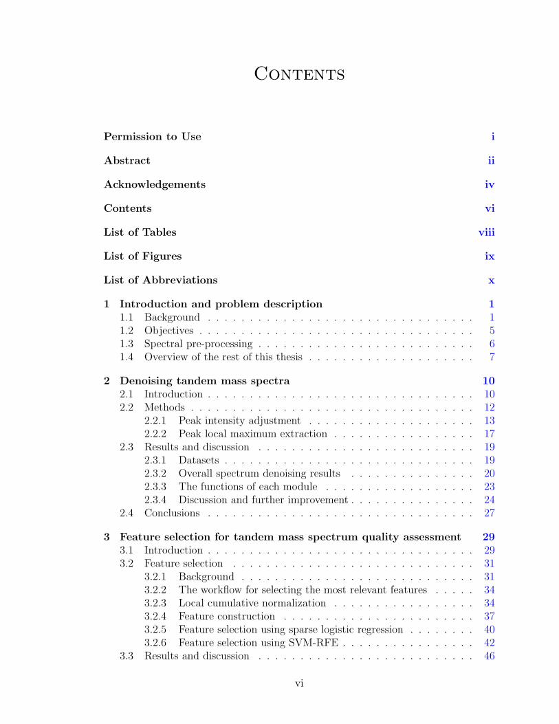
Contents

Permission to Use i

Abstract ii

Acknowledgements iv

Contents vi

List of Tables viii

List of Figures ix

List of Abbreviations x

1 Introduction and problem description 11.1 Background . . . . . . . . . . . . . . . . . . . . . . . . . . . . . . . . 11.2 Objectives . . . . . . . . . . . . . . . . . . . . . . . . . . . . . . . . . 51.3 Spectral pre-processing . . . . . . . . . . . . . . . . . . . . . . . . . . 61.4 Overview of the rest of this thesis . . . . . . . . . . . . . . . . . . . . 7

2 Denoising tandem mass spectra 102.1 Introduction . . . . . . . . . . . . . . . . . . . . . . . . . . . . . . . . 102.2 Methods . . . . . . . . . . . . . . . . . . . . . . . . . . . . . . . . . . 12

2.2.1 Peak intensity adjustment . . . . . . . . . . . . . . . . . . . . 132.2.2 Peak local maximum extraction . . . . . . . . . . . . . . . . . 17

2.3 Results and discussion . . . . . . . . . . . . . . . . . . . . . . . . . . 192.3.1 Datasets . . . . . . . . . . . . . . . . . . . . . . . . . . . . . . 192.3.2 Overall spectrum denoising results . . . . . . . . . . . . . . . 202.3.3 The functions of each module . . . . . . . . . . . . . . . . . . 232.3.4 Discussion and further improvement . . . . . . . . . . . . . . . 24

2.4 Conclusions . . . . . . . . . . . . . . . . . . . . . . . . . . . . . . . . 27

3 Feature selection for tandem mass spectrum quality assessment 293.1 Introduction . . . . . . . . . . . . . . . . . . . . . . . . . . . . . . . . 293.2 Feature selection . . . . . . . . . . . . . . . . . . . . . . . . . . . . . 31

3.2.1 Background . . . . . . . . . . . . . . . . . . . . . . . . . . . . 313.2.2 The workflow for selecting the most relevant features . . . . . 343.2.3 Local cumulative normalization . . . . . . . . . . . . . . . . . 343.2.4 Feature construction . . . . . . . . . . . . . . . . . . . . . . . 373.2.5 Feature selection using sparse logistic regression . . . . . . . . 403.2.6 Feature selection using SVM-RFE . . . . . . . . . . . . . . . . 42

3.3 Results and discussion . . . . . . . . . . . . . . . . . . . . . . . . . . 46

vi

3.3.1 Experimental datasets . . . . . . . . . . . . . . . . . . . . . . 463.3.2 Training and performance evaluation . . . . . . . . . . . . . . 473.3.3 Feature selected by SLR and the classification results . . . . . 483.3.4 Features selected by SVM-RFE and the classification results . 51

3.4 The most relevant feature set . . . . . . . . . . . . . . . . . . . . . . 54

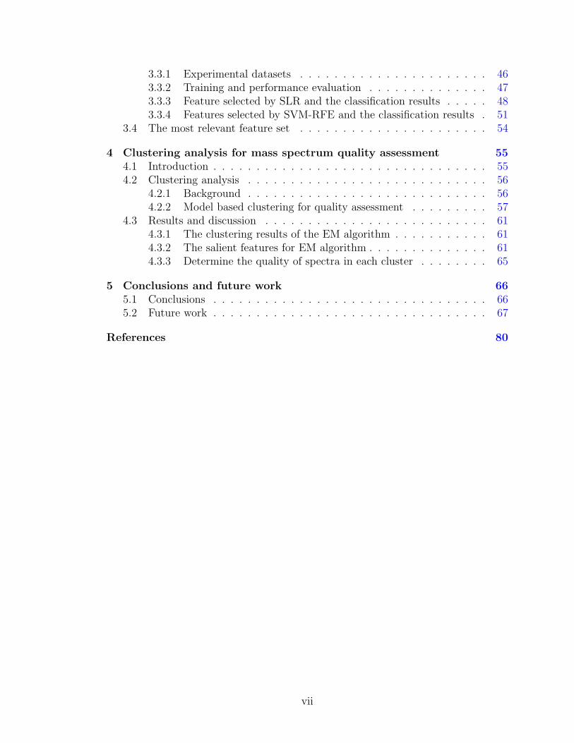
4 Clustering analysis for mass spectrum quality assessment 554.1 Introduction . . . . . . . . . . . . . . . . . . . . . . . . . . . . . . . . 554.2 Clustering analysis . . . . . . . . . . . . . . . . . . . . . . . . . . . . 56

4.2.1 Background . . . . . . . . . . . . . . . . . . . . . . . . . . . . 564.2.2 Model based clustering for quality assessment . . . . . . . . . 57

4.3 Results and discussion . . . . . . . . . . . . . . . . . . . . . . . . . . 614.3.1 The clustering results of the EM algorithm . . . . . . . . . . . 614.3.2 The salient features for EM algorithm . . . . . . . . . . . . . . 614.3.3 Determine the quality of spectra in each cluster . . . . . . . . 65

5 Conclusions and future work 665.1 Conclusions . . . . . . . . . . . . . . . . . . . . . . . . . . . . . . . . 665.2 Future work . . . . . . . . . . . . . . . . . . . . . . . . . . . . . . . . 67

References 80

vii

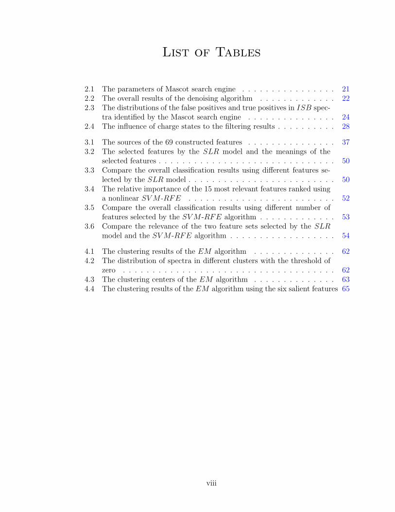
List of Tables

2.1 The parameters of Mascot search engine . . . . . . . . . . . . . . . . 212.2 The overall results of the denoising algorithm . . . . . . . . . . . . . 222.3 The distributions of the false positives and true positives in ISB spec-

tra identified by the Mascot search engine . . . . . . . . . . . . . . . 242.4 The influence of charge states to the filtering results . . . . . . . . . . 28

3.1 The sources of the 69 constructed features . . . . . . . . . . . . . . . 373.2 The selected features by the SLR model and the meanings of the

selected features . . . . . . . . . . . . . . . . . . . . . . . . . . . . . . 503.3 Compare the overall classification results using different features se-

lected by the SLR model . . . . . . . . . . . . . . . . . . . . . . . . . 503.4 The relative importance of the 15 most relevant features ranked using

a nonlinear SV M -RFE . . . . . . . . . . . . . . . . . . . . . . . . . 523.5 Compare the overall classification results using different number of

features selected by the SV M -RFE algorithm . . . . . . . . . . . . . 533.6 Compare the relevance of the two feature sets selected by the SLR

model and the SV M -RFE algorithm . . . . . . . . . . . . . . . . . . 54

4.1 The clustering results of the EM algorithm . . . . . . . . . . . . . . 624.2 The distribution of spectra in different clusters with the threshold of

zero . . . . . . . . . . . . . . . . . . . . . . . . . . . . . . . . . . . . 624.3 The clustering centers of the EM algorithm . . . . . . . . . . . . . . 634.4 The clustering results of the EM algorithm using the six salient features 65

viii

List of Figures

1.1 The fragment pattern of the peptide GPNAF (a) and a artificialspectrum of this peptide (b) . . . . . . . . . . . . . . . . . . . . . . . 3

1.2 The workflow of pre-processing tandem mass spectra . . . . . . . . . 8

2.1 An example of morphological reconstruction filter . . . . . . . . . . . 182.2 Venn diagram showing the overlap between the identified spectra from

the raw spectra and the denoised spectra . . . . . . . . . . . . . . . . 232.3 The number of spectra whose Mascot ion scores are larger than a given

value . . . . . . . . . . . . . . . . . . . . . . . . . . . . . . . . . . . . 25

3.1 The workflow of feature selection and its verification . . . . . . . . . . 353.2 (a) The feature selection frequency and (b) the absolute values of

mean weights in the twenty-five runs . . . . . . . . . . . . . . . . . . 49

4.1 Plot of the absolute values of clustering center difference in descendingorder . . . . . . . . . . . . . . . . . . . . . . . . . . . . . . . . . . . . 64

5.1 The new workflow for pre-processing tandem mass spectra . . . . . . 68

ix

List of Abbreviations

SV M Support vector machineSV M -RFE Recursive feature elimination based on support vector ma-

chineOSH Optimal separating hyperplaneLR Logistic regressionSLR Sparse logistic regressionEM Expectation maximizationLDA Linear discriminative analysisFLDA Fisher linear discriminative analysisMS/MS Tandem mass spectrometryTh Thompson, the unit of mass-to-charge ratioTIC Total ion currentTPR True positive rateTNR True negative rateFNR False negative rateROC Receiver operating characteristicAUC Area under the receiver operating characteristic curve

x

Chapter 1

Introduction and problem description

1.1 Background

Proteins are the primary components of living cells and accomplish most functions

of living cells [Hun93]. For example, some proteins define the shape and form of

cells. Other proteins may identify foreign substances and create an immune response,

turn genes on and off, function as enzymes to control chemical reactions in cells, or

transport oxygen, nutrients and wastes into and around cells etc. In molecular

biology, understanding the functions of proteins is the foundations of explanation.

The functions of proteins can be analyzed through their structures.

Proteins are long chain of amino acids. Each amino acid shares a basic structure:

a central carbon atom, an amino group (NH2), a carboxyl group (COOH), and a side

chain group (R). Different side chain groups define different amino acids. Generally,

all proteins are composed of the twenty standard amino acids. The amino acid

sequence of a protein is called its primary structure. The complex three-dimensional

structure of a protein controls its basic function. Protein sequencing, which aims

to determine the primary structures of proteins, is very important to determine the

three-dimensional structure of proteins.

In addition to analyzing the functions of proteins, protein sequencing is very

important to diagnose and treat diseases because doctors may need to analyze the

proteome - the whole proteins in a tissue at once. Therefore, the large scale sequenc-

ing of the whole proteins in a tissue is essential for us to find the biomarkers that

signal a disease, to find the targets for a drug and to find the medicines which suit

a specific person.

1

In practice, proteins can be thought of being composed of small multi-amino acid

subunits called peptides [KS00]. Therefore, for protein sequencing, we can sequence

several peptides of a protein. Then its whole sequence can be inferred. So peptide

sequencing is a key step in protein sequencing, and a central problem in proteomics

research, which is the large-scale analysis of proteins [AM03].

Nowadays, tandem mass spectrometry (MS/MS) is the method of choice for

peptide sequencing [NVA07]. After a protein is digested into peptides by proteases

like trypsin, a tandem mass spectrometer can measure the mass-to-charge ratio (m/z)

of a peptide ion, fragment the peptide ion, and measure the m/z of the fragment

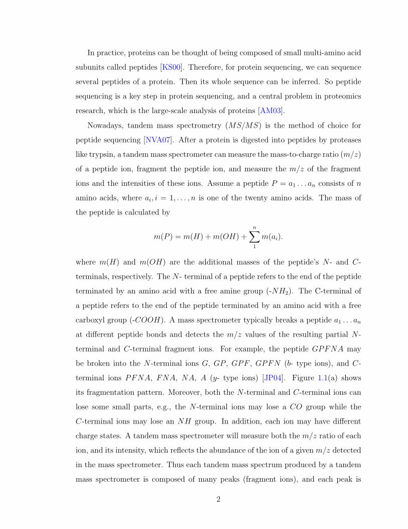
ions and the intensities of these ions. Assume a peptide P = a1 . . . an consists of n

amino acids, where ai, i = 1, . . . , n is one of the twenty amino acids. The mass of

the peptide is calculated by

m(P ) = m(H) + m(OH) +n∑1

m(ai).

where m(H) and m(OH) are the additional masses of the peptide’s N - and C-

terminals, respectively. The N - terminal of a peptide refers to the end of the peptide

terminated by an amino acid with a free amine group (-NH2). The C-terminal of

a peptide refers to the end of the peptide terminated by an amino acid with a free

carboxyl group (-COOH). A mass spectrometer typically breaks a peptide a1 . . . an

at different peptide bonds and detects the m/z values of the resulting partial N -

terminal and C-terminal fragment ions. For example, the peptide GPFNA may

be broken into the N -terminal ions G, GP , GPF , GPFN (b- type ions), and C-

terminal ions PFNA, FNA, NA, A (y- type ions) [JP04]. Figure 1.1(a) shows

its fragmentation pattern. Moreover, both the N -terminal and C-terminal ions can

lose some small parts, e.g., the N -terminal ions may lose a CO group while the

C-terminal ions may lose an NH group. In addition, each ion may have different

charge states. A tandem mass spectrometer will measure both the m/z ratio of each

ion, and its intensity, which reflects the abundance of the ion of a given m/z detected

in the mass spectrometer. Thus each tandem mass spectrum produced by a tandem

mass spectrometer is composed of many peaks (fragment ions), and each peak is

2

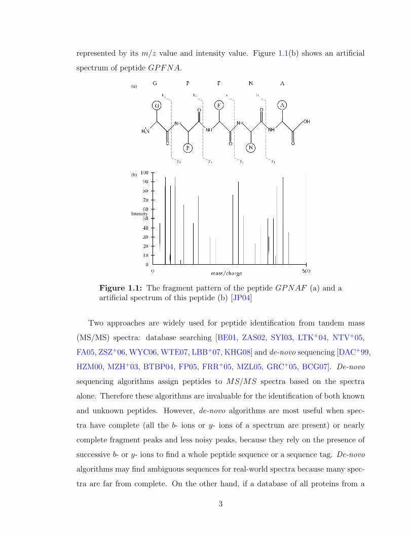
represented by its m/z value and intensity value. Figure 1.1(b) shows an artificial

spectrum of peptide GPFNA.

(a)

(b)

Intensity

Figure 1.1: The fragment pattern of the peptide GPNAF (a) and aartificial spectrum of this peptide (b) [JP04]

Two approaches are widely used for peptide identification from tandem mass

(MS/MS) spectra: database searching [BE01, ZAS02, SYI03, LTK+04, NTV+05,

FA05, ZSZ+06, WYC06, WTE07, LBB+07, KHG08] and de-novo sequencing [DAC+99,

HZM00, MZH+03, BTBP04, FP05, FRR+05, MZL05, GRC+05, BCG07]. De-novo

sequencing algorithms assign peptides to MS/MS spectra based on the spectra

alone. Therefore these algorithms are invaluable for the identification of both known

and unknown peptides. However, de-novo algorithms are most useful when spec-

tra have complete (all the b- ions or y- ions of a spectrum are present) or nearly

complete fragment peaks and less noisy peaks, because they rely on the presence of

successive b- or y- ions to find a whole peptide sequence or a sequence tag. De-novo

algorithms may find ambiguous sequences for real-world spectra because many spec-

tra are far from complete. On the other hand, if a database of all proteins from a

3

genome is accessible, peptides can be assigned to spectra by searching the peptides

in the database [JP04]. Database search based algorithms are currently the leading

peptide identification methods. Most database search approaches employ a score

function. Different search engines such as Sequest [EMY94] and Mascot [PPDC99]

adopt different scoring systems. Experiments show that using multiple search en-

gines may yield better results [KSC+05]. Therefore, some researchers have combined

the results of different search engines to assign peptides to spectra. For example, the

program Scaffold [EHFG05] assigns probabilities to the search results from differ-

ent peptide identification algorithms such as Mascot [PPDC99], Sequest [EMY94],

X!Tandem [CB04], Phenyx [CMG+03], Spectrum Mill (Agilent Technologies), and

OMSSA [GMK+04]. By using the above strategy, it is expected to improve the per-

formance of peptide identification from MS/MS spectra. However, with the steady

increase of the database size, more and more peptides similar to the one investigated

can be present in the searched database. On the other hand, the spectrum may

contain very few signal peaks or weak signal peaks whose intensities are indistin-

guishable from those of noise peaks [GKPW03]. Spectral pre-processing, becomes

very important in today’s proteomics research to improve the reliability of assigning

peptides to spectra.

Tandem mass spectrum pre-processing aims at processing spectra produced by

tandem mass spectrometers to increase both the accuracy and efficiency of subse-

quent peptide identification from spectra [HKPM06, NVA07]. Five types of pre-

processing methods are widely used: spectrum normalization [BGMY04, NP06,

DSZW08], spectrum clustering [FBS+08, FMH+07], precursor charge determina-

tion [SED+02, KWMN05, TSS+06, SHH08, NPL08, ZDSW08], spectrum denois-

ing [BCG+02, RCA+04, KL07, ZHL+08, DSPW09], and spectrum quality assess-

ment [PKK04, BGMY04, NRG+06, FMV+06, SMF+06, CT07, WGDP08, WDP08,

ZWDP09]. It is believed that these pre-processing algorithms can increase the num-

ber of identified peptides and improve the reliability of peptide identification from

tandem mass spectra. Now, spectral pre-processing has become a critical module in

many high throughput data processing pipelines. Both database search and de-novo

4

peptide identification algorithms can benefit from these pre-processing methods. Be-

cause these pre-processing algorithms increase the number of identified peptide, and

save much time for peptide identification from tandem mass spectra, they are par-

ticularly useful for the design of real-time control methodologies for tandem mass

spectrometers.

Nowadays, to improve the throughput and efficiency of mass spectrometry, re-

searchers try to design real-time control methodologies for mass spectrometers. Here

the timing is critical because we want to identify peptides and proteins in the process

of a tandem mass spectrometry experiment in a very short time period. One of the

key modules of the methodologies is spectral quality assessment which tries to objec-

tively determine the quality of spectra, and the poor quality spectra which are not

interpretable by peptide identification algorithms are removed from further analysis.

Because only high quality spectra are further analyzed by peptide identification algo-

rithms, we can save the time wasted in searching the poor quality spectra. However,

other pre-processing schemes are also important for the design of these real-time

control methodologies. For example, denoising methods remove most noisy peaks.

Thus the denoised spectra have far fewer noisy peaks than the undenoised spectra,

and the process of assigning peptides to spectra can be accelerated by using the de-

noised spectra instead of the original spectra. On the other hand, the signal-to-noise

ratios of spectra are increased because most noisy peaks are removed. The reliability

of assigning peptides to spectra is also improved.

1.2 Objectives

Pre-processing tandem mass spectra is a very important module for developing real-

time control methods of tandem mass spectrometers. The objective of this research

is to develop methods for pre-processing tandem mass spectra. Specifically in this

thesis we will present:

(1) A novel denoising method to filter out the noise in the tandem mass spectra

and thus to improve their quality.

5

(2) Feature selection methods to select the most relevant features for describing

the quality of tandem mass spectra.

(3) Quality assessment methods to classify tandem mass spectra into high quality

and poor quality.

1.3 Spectral pre-processing

Generally, spectral pre-processing methods can be divided into low level and high

level methods [HMA06]. The low level methods transform the continuous spectral

data (raw data) from mass spectrometers into list of peaks. These low level methods

may include peak centroiding, noise filtering, calibration, deisotoping, and decon-

volution. However, most raw data are processed directly by instruments’ software.

In this study we concentrate on high level pre-processing methods which are often

performed on the peak lists. Widely used high level pre-processing methods include

spectral clustering, precursor ion charge determination, spectral intensity normaliza-

tion, denoising, and automatic quality assessment of tandem mass spectra.

Spectral clustering algorithms detect spectra that are produced by the same pep-

tide and replace them with only one representative spectrum [FBS+08, TMW+03]. In

tandem mass spectrometry experiments, some spectra are generated from the same

peptide. When spectra are collected from a number of runs, the spectra from one

peptide may be recorded thousands of times. After clustering analysis, we can use

a single representative spectrum to represent all spectra produced by the same pep-

tide. Analyzing only representative spectra results in significant speedup of MS/MS

database searches.

Automatic charge state determination of precursor ions can save a lot of time of

peptide identification algorithms. For most database search based peptide identifi-

cation algorithms, when the accurate charge state of the precursor ion of a spectrum

is not known, the spectrum is searched multiple times assuming different charge

states. This blind strategy double or multiple the search time of peptide identifi-

cation algorithms. Nowadays, many algorithms try to determine the charge state

6

of the precursor ions [CMD+03, KWMN05, NPL08, TSS+06, ZDSW08]. For high

resolution spectra, digital signal processing based methods are widely used to pre-

dict the charge states of precursor ions; for low resolution spectra, machine learning

based algorithms are good choices.

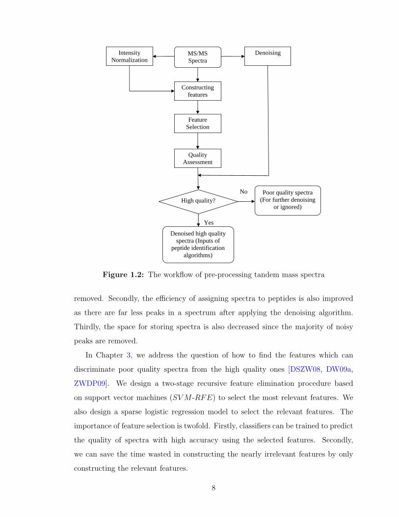
This thesis focus on denoising tandem mass spectra, feature construction and

feature selection, and quality assessment of tandem mass spectra. The whole work-

flow is given in Figure 1.2. For a typical tandem mass spectrum, about 80% of

peaks are noisy peaks [KL07]. Therefore, denoising algorithms are needed to remove

these noisy peaks. In addition, about 85% of spectra produced by spectrometers are

poor quality spectra which can’t be identified by peptide identification algorithms

[WGDP08]. So quality assessment algorithms are needed to remove these poor qual-

ity spectra before peptide identification. For quality assessment, we should construct

the relevant features which can discriminate high quality spectra from poor quality

ones. Therefore, in this thesis we design feature selection algorithms to select those

most relevant features out of the constructed features found in the literature. The

intensities of tandem mass spectra are normalized because some of these features use

the intensity information of peaks. Note that for the spectra from the same type

of tandem mass spectrmeters, these spectra share some properties. Therefore, some

features may represent the quality of this type of spectra, and for this reason, one

may find a small number of highly relevant features for this type of tandem mass

spectra. In other words, the feature selection module can be used only once for each

type of tandem mass spectrometers. After pre-processing, we can both speedup and

improve the reliability of assigning peptides to spectra.

1.4 Overview of the rest of this thesis

In Chapter 2, we discuss denoising tandem mass spectra [DSPW09]. The novel

contribution is that we design a spectral denoising algorithm to remove most noisy

peaks among a spectrum. The function of a denoising algorithm is threefold. Firstly,

the reliability of assigning peptides to spectra is improved as most noisy peaks are

7

Intensity Normalization

Quality Assessment

Feature Selection

Constructing features

Denoising

High quality?

Yes

No

MS/MS Spectra

Poor quality spectra (For further denoising

or ignored)

Denoised high quality spectra (Inputs of

peptide identification algorithms)

Figure 1.2: The workflow of pre-processing tandem mass spectra

removed. Secondly, the efficiency of assigning spectra to peptides is also improved

as there are far less peaks in a spectrum after applying the denoising algorithm.

Thirdly, the space for storing spectra is also decreased since the majority of noisy

peaks are removed.

In Chapter 3, we address the question of how to find the features which can

discriminate poor quality spectra from the high quality ones [DSZW08, DW09a,

ZWDP09]. We design a two-stage recursive feature elimination procedure based

on support vector machines (SV M -RFE) to select the most relevant features. We

also design a sparse logistic regression model to select the relevant features. The

importance of feature selection is twofold. Firstly, classifiers can be trained to predict

the quality of spectra with high accuracy using the selected features. Secondly,

we can save the time wasted in constructing the nearly irrelevant features by only

constructing the relevant features.

8

In Chapter 4, we discuss cluster analysis for quality assessment of tandem mass

spectra [DW09b, DSW09, WDP08]. We use the model based clustering technique

for the quality assessment of tandem mass spectra. After removing the poor qual-

ity spectra, much time can be saved for peptide identification algorithms by not

searching the poor quality spectra. In addition, the number of false positives is also

decreased since most poor quality spectra are removed.

In Chapter 5, we conclude this thesis and give some directions for further im-

provement.

9

Chapter 2

Denoising tandem mass spectra

2.1 Introduction

Tandem mass spectrometers are powerful tools for the analysis of biological com-

plexes. In a typical tandem mass spectrometry experiment, proteins are first ex-

tracted from a biological complex. Then after a protein is digested into peptides by

proteases like trypsin, a tandem mass spectrometer measures the intensities of pep-

tide ions and fragment ions versus their mass to charge ratio (m/z) which are called

mass spectra. Tandem mass spectrometry is a complex method, and well-trained

experts are needed to analyze the produced spectra [Cha]. Tandem mass spectrome-

try is also a high-throughput analytical method, and it can produce a large number

of tandem mass spectra. In a typical tandem mass spectrum, up to 80% peaks are

noise [KL07]. These noisy peaks may be derived from chemical, electrical or other

sources. Therefore, it is beneficial to apply a spectrum denoising method before

assigning peptides to spectra. By removing most noisy peaks, the reliability of as-

signing peptides to spectra can be improved. In addition, since most noise peaks are

removed, the speed of assigning peptides to spectra may also be increased.

Spectrum denoising methods intend to keep signal peaks (reflecting peptide frag-

ment ions) while removing noisy peaks (not reflecting peptide fragment ions). In fact,

most peptide identification algorithms adopt denoising methods as a pre-processing

step. For example, PEAKS [MZL05], PepNovo [FP05] and AUDENS [GRC+05] all

have their own denoising models. However, there are many ad hoc problems for

spectrum denoising issues. Firstly, the property of un-equally spaced m/z values of

spectra makes it improper to directly use any standard denoising algorithms for tra-

10

ditional signal processing [MRH+06]. Secondly, the noise in a spectrum are hardly

modeled by a single statistical model. For example, most noisy peaks are in the

middle of m/z range of a spectrum, and accordingly, far fewer noisy peaks are in the

two ends of a spectrum [KL07]. Besides, the peaks in the middle of m/z range tend

to have higher intensities than those at the two ends.

Generally, there exist three types of spectrum denoising algorithms: thresh-

old, digital signal processing, and machine learning or heuristic search algorithms.

Threshold methods simply discard peaks with intensities below a threshold. How-

ever, the thresholds are hard to determine because a global optimal threshold may

not exist for an algorithm to work well. Moreover, these methods only use the in-

tensity information of each peak to determine whether a peak is a fragment ion or

a noisy peak. These methods implicitly assume the independence of peaks without

considering the interrelationship. In fact, a true fragment ion may be related to other

fragment ions in a true tandem mass spectrum. For example, the mass difference of

two signal ions may be equal to the mass of one of the 20 amino acids, e.g., bi, bi+1

ions.

The second type of methods uses digital signal processing procedures such as

Fourier analysis and wavelet analysis for denoising spectra [RCA+04, MRH+06].

Digital signal processing methods are successfully used in other fields such as speech

recognition, image processing, and computer vision. However, these methods assume

that the m/z difference between peaks is a constant (interpolation is used to produce

equally spaced m/z values at the expense of introducing extra peaks). Indeed, as

the noise is m/z dependent, short time Fourier transform or wavelet transform are

better choices than Fourier transform [Mal99]. These methods reduce the intensities

of the “noisy” peaks without removing them. As with threshold methods, digital

signal processing methods use the intensity information only.

The third type of methods is based on machine learning, or some heuristic

search using not only intensity information of peaks but also some additional in-

formation contained in a spectrum, such as isotopic ions or complementary ions

[BCG+02, ZHL+08]. However, noise are neither equally distributed in the whole

11

m/z range of a spectrum, nor equally distributed among features extracted from a

spectrum used for machine learning. As a result, the noise may degenerate the per-

formance of classifiers, and this type of method may not perform as well as expected.

Therefore, we need novel denoising algorithms which are more robust than threshold

methods, do not need to introduce extra pseudo peaks, and are “adaptive” to the

m/z dependence properties of noise in a spectrum.

In this chapter, we present a spectral denoising algorithm which partially solves

the above mentioned shortcomings of previous denoising algorithms. The proposed

algorithm first adjusts the intensities of the peaks of a spectrum using several fea-

tures extracted. Then the algorithm removes the fragment ions whose intensities

are not the local maxima of the intensity-adjusted spectrum using a morphological

reconstruction filter [Vin93]. Experiments are conducted on two ion trap mass spec-

tral datasets, and the results show that our algorithm can remove about 69% of the

peaks which are likely noisy peaks among a spectrum. At the same time, the number

of spectra that can be identified by Mascot increases by 31.23% and 14.12% for the

spectra from two datasets.

2.2 Methods

In this study, a spectrum S with N peaks is represented by the peak list, i.e.,

S = {(xk, ik) | xk ∈ R+, ik ∈ R+, 1 ≤ k ≤ N}

where (xk, ik) denotes peak k with m/z value of xk and intensity of ik.

The proposed spectral denoising method consists of two unique modules: peak

intensity adjustment and intensity local maximum extraction. The first module

is used to adjust the intensities of signal peaks in a spectrum. After adjustment,

intensities of signal peaks are expected to be the local maxima in a spectrum. The

second module is used to select these local maxima of the signal peak intensity-

adjusted spectra, and thus peaks whose intensities are not the local maxima are

removed.

12

2.2.1 Peak intensity adjustment

The intensity is an important attribute of a peak in a spectrum. The empirical

approaches usually assume that peaks with high intensities are more likely to be

signal peaks than those with low intensities. However, there are many exceptions to

these approaches. Thus to distinguish signal peaks from noisy peaks, more attributes

of peaks should be taken into consideration. For example, signal peaks may have

complementary peaks whose masses are added to the signal peaks to give the mass

of a precursor ion.

Five features are constructed for each peak on the basis of the properties of

theoretical peptide mass spectra [WGDP08]. A score for each peak is calculated by

a linear combination of these features. To define these features, as in [WGDP08],

four variables are introduced

dif1(x, y) = x− y

dif2(x, y) = x− (y + 1)/2

sum1(x, y) = x + y

sum2(x, y) = x + (y + 1)/2

For a peak (x, i) (for simplicity, this peak is called peak x) of a spectrum S,

the first feature F1 collects the number of peaks whose mass differences with x

approximately equal the mass of one of the twenty amino acids.

F1(x) = |{y | abs(dif1(x, y)) ≈ Mi or

abs(dif1(x, y)) ≈ Mi/2 or

abs(dif2(x, y)) ≈ Mi/2 or

abs(dif2(y, x)) ≈ Mi/2}|

where | • | is the cardinality of a set; abs is the absolute value function; and Mi(i =

1, 2, . . . , 20) is the mass of one of the twenty amino acids. In this study we consider all

Methionine amino acids to be sulfoxidized and do not distinguish three pairs of amino

13

acids by their masses: isoleucine vs. leucine, glutamine vs. lysine, and sulfoxidized

methionine vs. phenylalanine as the masses of each pair are very close. If both peaks

x and y are singly charged, their difference equals the mass of one of the 20 amino

acids, and abs(dif1(x, y)) ≈ Mi; if both x and y are doubly charged, their difference

equals half of the mass of one of the 20 amino acid, and abs(dif1(x, y)) ≈ Mi/2; if

x is singly charged while y is doubly charged, abs(dif2(x, y)) equals half of one of

the mass of the 20 amino acids; and if x is doubly charged while y is singly charged,

abs(dif2(y, x)) equals half of the mass of one of the 20 amino acids. The comparison

implied by ≈ uses a tolerance. Bern et al used ±0.37 [BGMY04] for constructing

features for the quality assessment of ion trap tandem mass spectra. Wong et al used

±0.3 for fragment ion mass tolerance, and ±1 for precursor ion mass tolerance for

ion trap tandem mass spectra [WSCC07]. In this study, we use ±0.8 for fragment ion

mass tolerance, and ±2 for precursor ion mass tolerance because these parameters

seem to be reasonable for ion trap spectra for the Mascot search engine to give good

peptide identification results.

The second feature F2 collects the number of peaks whose masses added to x

approximately equal the mass of the precursor ion.

F2(x) = |{y | sum1(x, y) ≈ Mparent + 2 ∗MH or

sum1(x, y) ≈ Mparent/2 + 2 ∗MH or

sum2(x, y) ≈ Mparent/2 + 2 ∗MH or

sum2(y, x) ≈ Mparent/2 + 2 ∗MH}|

where Mparent is the mass of the precursor ion (parent), and MH is the mass of a

hydrogen atom. As for F1, if both peaks x and y are singly charged, sum1(x, y) ≈Mparent+2∗MH ; if both x and y are doubly charged, sum1(x, y) ≈ Mparent/2+2∗MH ;

if x is singly charged while y is doubly charged, sum2(x, y) ≈ Mparnet/2 + 2 ∗MH ;

and if x is doubly charged while y is singly charged, sum2(y, x) ≈ Mparnet/2+2∗MH .

The third feature F3 collects the number of peaks which are produced by losing

14

a water or an ammonia molecule from x.

F3(x) = |{y | dif1(x, y) ≈ Mwater or Mammonia or

dif1(x, y) ≈ Mwater/2 or Mammonia/2 or

dif2(x, y) ≈ Mwater/2 or Mammonia/2 or

−dif2(y, x) ≈ Mwater/2 or Mammonia/2}|

where Mwater is the mass of a water molecule and Mammonia is the mass of an ammonia

molecule. Because x loses a molecule to form y, x should be larger than y if they have

the same charge state. Therefore, as opposed to F1, the abs function should not be

used here. If both peaks x and y are singly charged, dif1(x, y) ≈ Mwater or Mammonia;

if both x and y are doubly charged, dif1(x, y) ≈ Mwater/2 or Mammonia/2; if x is

singly charged while y is doubly charged, dif2(x, y) ≈ Mwater/2 or Mammonia/2; and

if x is doubly charged while y is singly charged, a minus sign should be added to

dif2(y, x) and −dif2(y, x) ≈ Mwater/2 or Mammonia/2.

The fourth feature collects the number of peaks which are produced by losing a

CO group or an NH group from x.

F4(x) = |{y | dif1(x, y) ≈ MCO or MNH or

dif1(x, y) ≈ MCO/2 or MNH/2 or

dif2(x, y) ≈ MCO/2 or MNH/2 or

−dif2(y, x) ≈ MCO/2 or MNH/2}|

where MCO and MNH are the mass of a CO group and an NH group, respectively.

For the same reason as for F3, x should be larger than y if they have the same

charge state. Therefore, if both peaks x and y are singly charged, dif1(x, y) ≈MCO or MNH ; if both x and y are doubly charged, dif1(x, y) ≈ MCO/2 or MNH/2;

if x is singly charged while y is doubly charged, dif2(x, y) ≈ MCO/2 or MNH/2;

and if x is doubly charged while y is singly charged, the two peaks should satisfy

−dif2(y, x) ≈ MCO/2 or MNH/2. The fifth feature is used to collect the number of

isotope peaks associated with x

F5(x) = |{y | x ≈ y − 1 or x ≈ y − 0.5)}|

15

The adjusted intensity of each peak is the original intensity of the peak multiplied

by the score computed based on the five features. The final score for peak x is

calculated as:

Score(x) = ω0 + ω1 ∗ f1(x) + ω2 ∗ f2(x) + ω3 ∗ f3(x) + ω4 ∗ f4(x) + ω5 ∗ f5(x)

where fi(i = 1, . . . , 5) is the normalized value of each feature (normalized to have

the mean of zero and the variance of one), and ωi(i = 0, . . . , 5) is a coefficient. This

study sets the bias ω0 = 5 to ensure only few peaks have negative score; ω1 and

ω2 are set to 1.0; both ω3 and ω4 are set to 0.2; and ω5 is set to 0.5. These values

are selected according to the normalization method of the Sequest algorithm. In

this algorithm, a magnitude of 50 is assigned to the b- and y- ions in a theoretical

spectrum. The neutral loss of water ions, the neutral loss of ammonia ions, and a-

ions are assigned a value of 10. The ions which have mass difference of ±1 with b- and

y- ions are assigned a value of 25. In this study the values are slightly different from

those of the Sequest algorithm to avoid numerical problems incurred by multiplying

large numbers, but the relative importance of the value of each parameter is the

same as the value of the Sequest search engine. Note that the Sequest algorithm

does not consider complementary ions. However, from the study of other peptide

identification algorithms such as Mascot and our own study, the complement ions

are very likely to be signal peaks, e.g., the presence of complementary ions is a

very important feature to predict whether a spectrum is of high or poor quality

[WGDP08, DSZW08]. Therefore, the weight value for feature F2 is assigned the

same as that for feature F1. The score function is similar to linear discriminative

analysis (LDA) which combines a finite number of features into a score [DHS00].

This study does not use these features to train a classifier to classify a peak as

a signal peak or a noisy peak because of the peak distribution properties of tandem

mass spectra. For example, the number of peaks in the middle of m/z value range

of a spectrum is larger than the number of peaks in the two ends of the spectrum,

and most noisy peaks are in the middle of m/z value range. Thus the features

we constructed are m/z dependent. In addition, the masses of peptides are widely

16

scattered, and the number of peaks of spectra are quite different. These are all

challenges for machine learning algorithms. Elaborate normalization methods are

necessary before using these algorithms.

The intensities of signal peaks are increased while the intensities of noisy peaks

are decreased after peak intensity adjustment. However, using a simple threshold is

still not effective to differentiate signal peaks from noisy peaks because the scores of

peaks in a spectrum tend to be larger in the middle of the m/z range than the scores

of the two end peaks because most noisy peaks are in the middle of the m/z range

of a spectrum. It is more reasonable to assume that the noisy peaks in a narrow

m/z range are equally distributed, and that the signal peaks are mostly the local

maxima of a spectrum after peak intensity adjustment. Therefore, noisy peaks can

be removed by keeping only these local maxima.

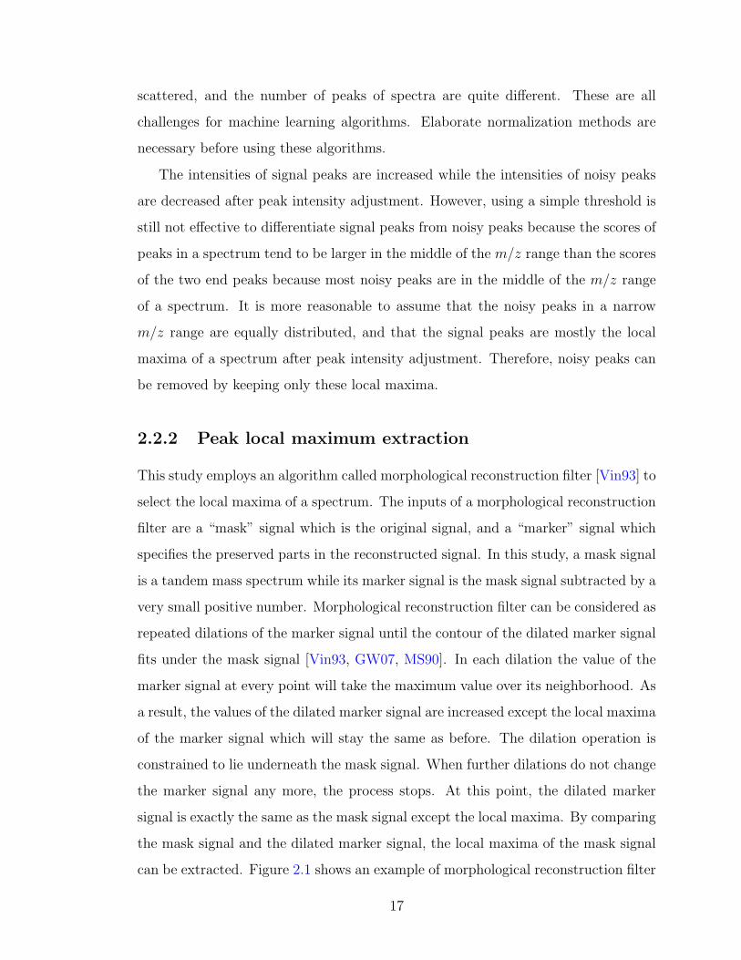
2.2.2 Peak local maximum extraction

This study employs an algorithm called morphological reconstruction filter [Vin93] to

select the local maxima of a spectrum. The inputs of a morphological reconstruction

filter are a “mask” signal which is the original signal, and a “marker” signal which

specifies the preserved parts in the reconstructed signal. In this study, a mask signal

is a tandem mass spectrum while its marker signal is the mask signal subtracted by a

very small positive number. Morphological reconstruction filter can be considered as

repeated dilations of the marker signal until the contour of the dilated marker signal

fits under the mask signal [Vin93, GW07, MS90]. In each dilation the value of the

marker signal at every point will take the maximum value over its neighborhood. As

a result, the values of the dilated marker signal are increased except the local maxima

of the marker signal which will stay the same as before. The dilation operation is

constrained to lie underneath the mask signal. When further dilations do not change

the marker signal any more, the process stops. At this point, the dilated marker

signal is exactly the same as the mask signal except the local maxima. By comparing

the mask signal and the dilated marker signal, the local maxima of the mask signal

can be extracted. Figure 2.1 shows an example of morphological reconstruction filter

17

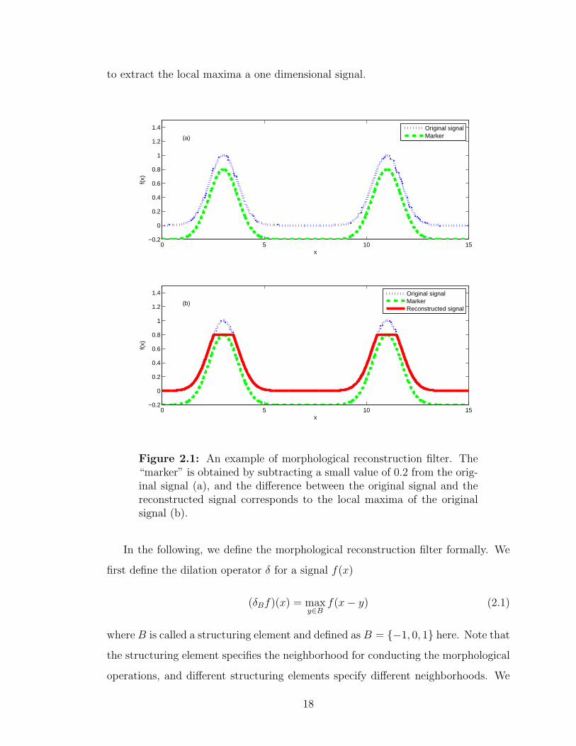
to extract the local maxima a one dimensional signal.

0 5 10 15−0.2

0

0.2

0.4

0.6

0.8

1

1.2

1.4

x

f(x)

(a)

Original signalMarker

0 5 10 15−0.2

0

0.2

0.4

0.6

0.8

1

1.2

1.4

x

f(x)

(b)

Original signalMarkerReconstructed signal

Figure 2.1: An example of morphological reconstruction filter. The“marker” is obtained by subtracting a small value of 0.2 from the orig-inal signal (a), and the difference between the original signal and thereconstructed signal corresponds to the local maxima of the originalsignal (b).

In the following, we define the morphological reconstruction filter formally. We

first define the dilation operator δ for a signal f(x)

(δBf)(x) = maxy∈B

f(x− y) (2.1)

where B is called a structuring element and defined as B = {−1, 0, 1} here. Note that

the structuring element specifies the neighborhood for conducting the morphological

operations, and different structuring elements specify different neighborhoods. We

18

further define elementary geodesic dilation as follows:

δ1gf = (δBf) ∧ (g) (2.2)

where ∧ standards for the pointwise minimum. The elementary geodesic dilation

operator prevents the processed signal from having larger values than the original

signal. Similarly, we define the geodesic dilation of size n as applying the elementary

geodesic dilation n times.

δng f = δn−1

g (δ1gf) (2.3)

The morphological reconstruction of g from f is defined as carrying out geodesic

dilation iteratively until stability is achieved.

ρgf =⋃n≥1

δng f (2.4)

Where f is the marker signal. Please see reference [Vin93] for details about the

morphological reconstruction filter.

2.3 Results and discussion

2.3.1 Datasets

This study employs two ion trap tandem mass spectral datasets: ISB dataset and

TOV dataset to investigate the performance of the introduced denoising algorithm.

The following is a brief description of these datasets.

(1) ISB dataset. The spectra in ISB dataset are acquired from a low reso-

lution ESI ion trap mass spectrometer as described in [KPN+02]. These spectra

consist of 22 LC/MS/MS runs produced by Institute of System Biology (ISB) from

18 control mixture proteins. There are a total of 37, 044 spectra in ISB dataset.

These spectra are searched using Mascot against the ipi.HUMAN.v3.48.fasta (taken

from EMBL-EBI, http://www.ebi.ac.uk/IPI/IPIhuman.html) containing 71, 399 se-

quences and 5 contaminant sequences (P00760, P00761, P02769, Q29443 and Q29463

19

from www.uniprot.org) appended with the sequences of the mixture proteins (from

www.uniprot.org).

(2) TOV dataset. The MS/MS spectra are acquired from a LCQ DECA XP ion

trap spectrometer (ThermoElectron Corp.) as described in [WGDP06]. The num-

ber of spectra in this dataset is 22, 576, and these spectra are searched using Mas-

cot against the ipi.HUMAN.v3.42.fasta (http://www.ebi.ac.uk/IPI/IPIhuman.html)

containing 72, 340 protein sequences and 5 contaminant sequences (P00760, P00761,

P02769, Q29443 and Q29463 from www.uniprot.org).

Similar to [MRH+06, GKPW03, ZHL+08], the Mascot search engine is used to

evaluate our denoising algorithm. The raw spectra (un-denoised spectra) and the

denoised spectra are searched using the Mascot search engine with the same pa-

rameters. The parameters used are given in Table 2.1. A spectrum is identified if

its Mascot ion score is larger than a certain threshold. Mascot can provide two

thresholds for each peptide: the homology threshold and the identity threshold

[BLY+07, LBB+07, FNC07] (Note: one can find both the identity threshold and

homology threshold for a spectrum by putting the cursor above the query number

of the Mascot search report). Each of these two thresholds is different for different

peptides. Most proteomics laboratories [BLY+07] use the identity threshold as the

cut-off value to expect that the false discover rate of the peptide identification is less

than (typically) 5%. In this study, we also adopt the identity threshold as the cut-off

value, i.e., a spectrum is identified if its Mascot ion score is larger than its identity

threshold. By doing so, the false discovery rate is expected to be less than 5% for

peptide identification from both the raw and denoised spectra.

2.3.2 Overall spectrum denoising results

Experiments are conducted on two ion trap tandem mass spectral datasets (ISB and

TOV ) to illustrate the performance of the proposed spectral denoising method by

comparing the Mascot search results from the raw datasets to those from the same

datasets denoised by the proposed method. The results of comparisons follow as:

Table 2.2 lists the overall results of experiments. From Table 2.2, the proposed

20

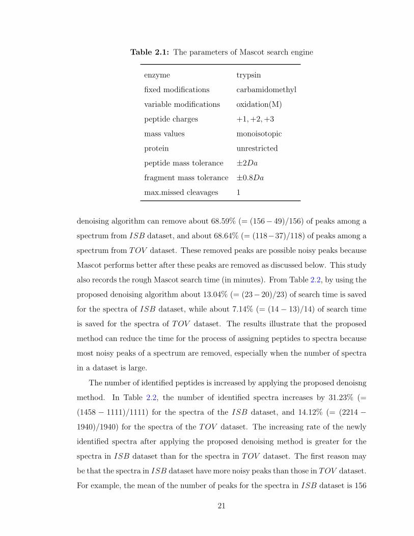
Table 2.1: The parameters of Mascot search engine

enzyme trypsin

fixed modifications carbamidomethyl

variable modifications oxidation(M)

peptide charges +1, +2, +3

mass values monoisotopic

protein unrestricted

peptide mass tolerance ±2Da

fragment mass tolerance ±0.8Da

max.missed cleavages 1

denoising algorithm can remove about 68.59% (= (156− 49)/156) of peaks among a

spectrum from ISB dataset, and about 68.64% (= (118−37)/118) of peaks among a

spectrum from TOV dataset. These removed peaks are possible noisy peaks because

Mascot performs better after these peaks are removed as discussed below. This study

also records the rough Mascot search time (in minutes). From Table 2.2, by using the

proposed denoising algorithm about 13.04% (= (23− 20)/23) of search time is saved

for the spectra of ISB dataset, while about 7.14% (= (14 − 13)/14) of search time

is saved for the spectra of TOV dataset. The results illustrate that the proposed

method can reduce the time for the process of assigning peptides to spectra because

most noisy peaks of a spectrum are removed, especially when the number of spectra

in a dataset is large.

The number of identified peptides is increased by applying the proposed denoisng

method. In Table 2.2, the number of identified spectra increases by 31.23% (=

(1458 − 1111)/1111) for the spectra of the ISB dataset, and 14.12% (= (2214 −1940)/1940) for the spectra of the TOV dataset. The increasing rate of the newly

identified spectra after applying the proposed denoising method is greater for the

spectra in ISB dataset than for the spectra in TOV dataset. The first reason may

be that the spectra in ISB dataset have more noisy peaks than those in TOV dataset.

For example, the mean of the number of peaks for the spectra in ISB dataset is 156

21

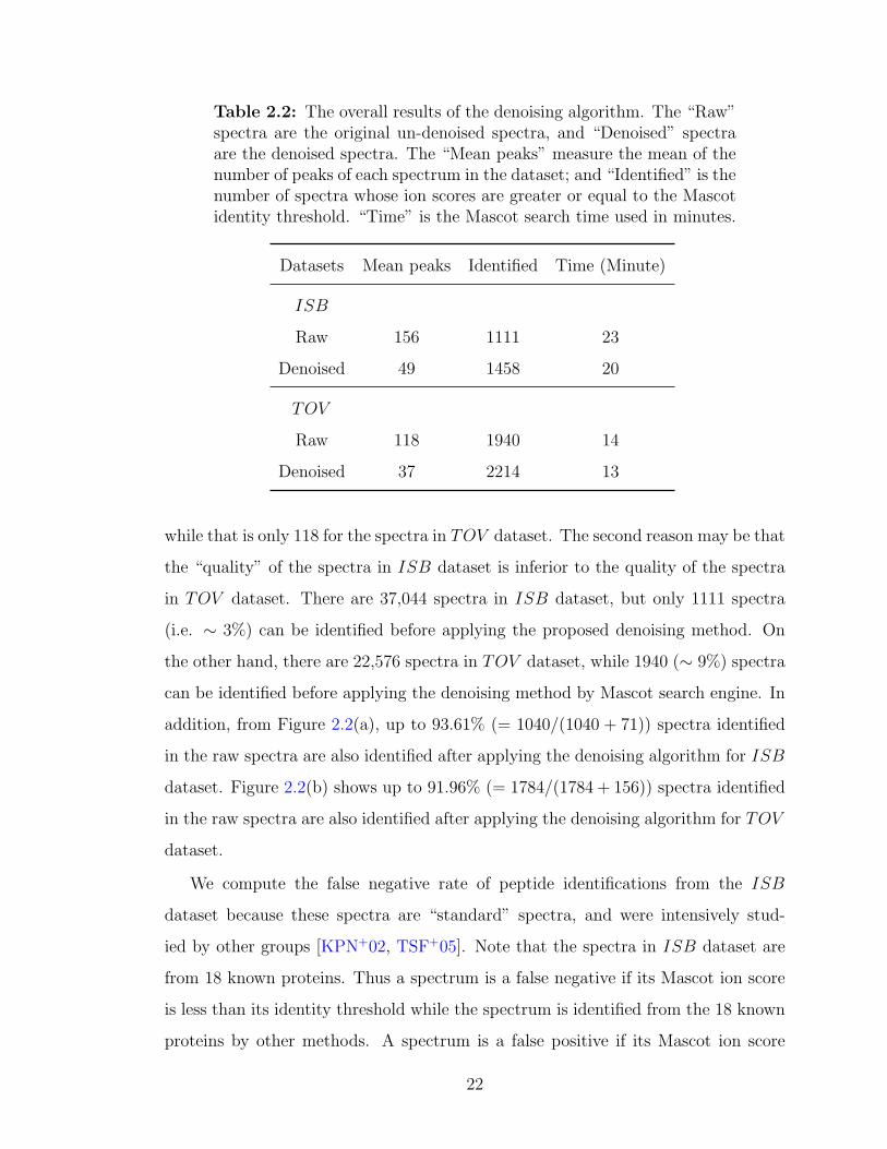
Table 2.2: The overall results of the denoising algorithm. The “Raw”spectra are the original un-denoised spectra, and “Denoised” spectraare the denoised spectra. The “Mean peaks” measure the mean of thenumber of peaks of each spectrum in the dataset; and “Identified” is thenumber of spectra whose ion scores are greater or equal to the Mascotidentity threshold. “Time” is the Mascot search time used in minutes.

Datasets Mean peaks Identified Time (Minute)

ISB

Raw 156 1111 23

Denoised 49 1458 20

TOV

Raw 118 1940 14

Denoised 37 2214 13

while that is only 118 for the spectra in TOV dataset. The second reason may be that

the “quality” of the spectra in ISB dataset is inferior to the quality of the spectra

in TOV dataset. There are 37,044 spectra in ISB dataset, but only 1111 spectra

(i.e. ∼ 3%) can be identified before applying the proposed denoising method. On

the other hand, there are 22,576 spectra in TOV dataset, while 1940 (∼ 9%) spectra

can be identified before applying the denoising method by Mascot search engine. In

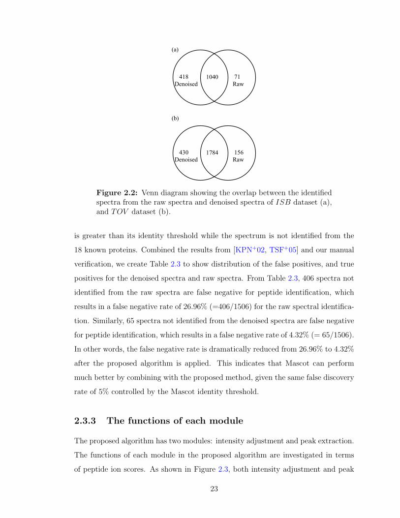
addition, from Figure 2.2(a), up to 93.61% (= 1040/(1040 + 71)) spectra identified

in the raw spectra are also identified after applying the denoising algorithm for ISB

dataset. Figure 2.2(b) shows up to 91.96% (= 1784/(1784 + 156)) spectra identified

in the raw spectra are also identified after applying the denoising algorithm for TOV

dataset.

We compute the false negative rate of peptide identifications from the ISB

dataset because these spectra are “standard” spectra, and were intensively stud-

ied by other groups [KPN+02, TSF+05]. Note that the spectra in ISB dataset are

from 18 known proteins. Thus a spectrum is a false negative if its Mascot ion score

is less than its identity threshold while the spectrum is identified from the 18 known

proteins by other methods. A spectrum is a false positive if its Mascot ion score

22

1040 71

Raw

418

Denoised

1784 156

Raw

430

Denoised

(a)

(b)

Figure 2.2: Venn diagram showing the overlap between the identifiedspectra from the raw spectra and denoised spectra of ISB dataset (a),and TOV dataset (b).

is greater than its identity threshold while the spectrum is not identified from the

18 known proteins. Combined the results from [KPN+02, TSF+05] and our manual

verification, we create Table 2.3 to show distribution of the false positives, and true

positives for the denoised spectra and raw spectra. From Table 2.3, 406 spectra not

identified from the raw spectra are false negative for peptide identification, which

results in a false negative rate of 26.96% (=406/1506) for the raw spectral identifica-

tion. Similarly, 65 spectra not identified from the denoised spectra are false negative

for peptide identification, which results in a false negative rate of 4.32% (= 65/1506).

In other words, the false negative rate is dramatically reduced from 26.96% to 4.32%

after the proposed algorithm is applied. This indicates that Mascot can perform

much better by combining with the proposed method, given the same false discovery

rate of 5% controlled by the Mascot identity threshold.

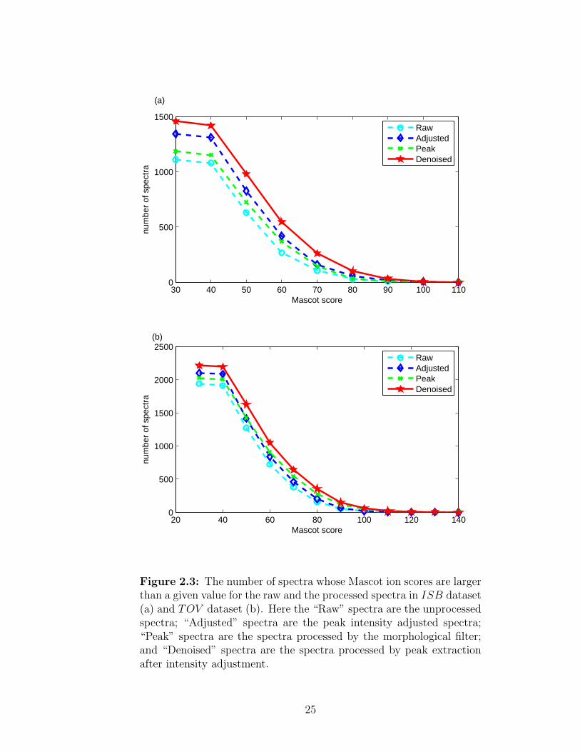
2.3.3 The functions of each module

The proposed algorithm has two modules: intensity adjustment and peak extraction.

The functions of each module in the proposed algorithm are investigated in terms

of peptide ion scores. As shown in Figure 2.3, both intensity adjustment and peak

23

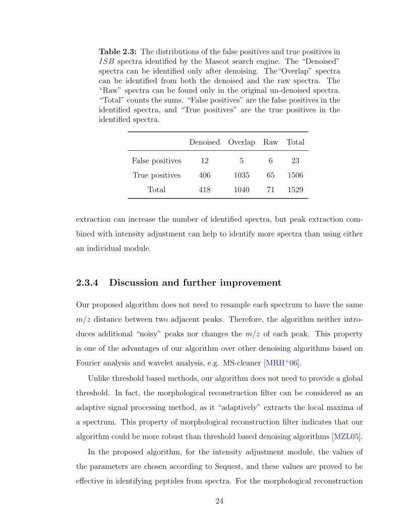
Table 2.3: The distributions of the false positives and true positives inISB spectra identified by the Mascot search engine. The “Denoised”spectra can be identified only after denoising. The“Overlap” spectracan be identified from both the denoised and the raw spectra. The“Raw” spectra can be found only in the original un-denoised spectra.“Total” counts the sums. “False positives” are the false positives in theidentified spectra, and “True positives” are the true positives in theidentified spectra.

Denoised Overlap Raw Total

False positives 12 5 6 23

True positives 406 1035 65 1506

Total 418 1040 71 1529

extraction can increase the number of identified spectra, but peak extraction com-

bined with intensity adjustment can help to identify more spectra than using either

an individual module.

2.3.4 Discussion and further improvement

Our proposed algorithm does not need to resample each spectrum to have the same

m/z distance between two adjacent peaks. Therefore, the algorithm neither intro-

duces additional “noisy” peaks nor changes the m/z of each peak. This property

is one of the advantages of our algorithm over other denoising algorithms based on

Fourier analysis and wavelet analysis, e.g. MS-cleaner [MRH+06].

Unlike threshold based methods, our algorithm does not need to provide a global

threshold. In fact, the morphological reconstruction filter can be considered as an

adaptive signal processing method, as it “adaptively” extracts the local maxima of

a spectrum. This property of morphological reconstruction filter indicates that our

algorithm could be more robust than threshold based denoising algorithms [MZL05].

In the proposed algorithm, for the intensity adjustment module, the values of

the parameters are chosen according to Sequest, and these values are proved to be

effective in identifying peptides from spectra. For the morphological reconstruction

24

20 40 60 80 100 120 1400

500

1000

1500

2000

2500

Mascot score

num

ber

of s

pect

ra

(b)

RawAdjustedPeakDenoised

30 40 50 60 70 80 90 100 1100

500

1000

1500

Mascot score

num

ber

of s

pect

ra

(a)

RawAdjustedPeakDenoised

Figure 2.3: The number of spectra whose Mascot ion scores are largerthan a given value for the raw and the processed spectra in ISB dataset(a) and TOV dataset (b). Here the “Raw” spectra are the unprocessedspectra; “Adjusted” spectra are the peak intensity adjusted spectra;“Peak” spectra are the spectra processed by the morphological filter;and “Denoised” spectra are the spectra processed by peak extractionafter intensity adjustment.

25

filter, there is only one parameter to choose. This parameter can be set as a very

small value, e.g., the smallest intensity difference between two peaks. While for the

methods based on wavelet analysis, one need to choose several parameters such as

the wavelet basis functions and the thresholds of the wavelet coefficients. These

parameters can significantly influence the final denoising results.

The proposed algorithm uses more information about a theoretical peptide frag-

ment ion in denoising spectra. We construct several features to adjust the intensities

of a peak. Although the intensities of peaks at the two ends of each spectrum are

less enhanced than those in the middle of m/z range, the intensities of signal peaks

are still enhanced more than those of the noisy peaks. Thus the signal peaks are

still local maxima of a spectrum, and the morphological reconstruction filter can

correctly discriminate the signal peaks from noisy ones. From this point of view, our

method is more robust than machine learning based denoising algorithms [ZHL+08]

because our algorithm decreases the influence of the unequally distributed noise in

tandem mass spectra.

The influence of the denoising method is different to the spectra with different

charge states. As shown in Table 2.4, Mascot can identify another 177 triply charged

spectra in ISB dataset after applying the proposed denoising algorithm, i.e., about

42.34% (= 177/418) of newly identified spectra are triply charged. The number

of triply charged spectra accounts for about 33.80% (= 24/71) of the lost spec-

tra. Therefore the proposed denoising method can help to find more triply charged

spectra. This phenomenon is more obvious for the spectra in TOV dataset. For

example, about 24.88% (= 107/430) of newly identified spectra are triply charged,

while only 12.82% (= 20/156) of spectra are triply charged of all the lost spectra af-

ter applying the denoising algorithm. While for singly charged spectra, although the

denoising method can increase the number of identified spectra, the singly charged

spectra account for about 15.49% (= 11/71) of the lost spectra. This number is rela-

tively large taking into consideration the small number of originally identified singly

charged spectra. Therefore, one can expect that a denoising algorithm which em-

ploys several properties of a tandem mass spectra (such as charge state and number

26

of peaks [ZHL+08]) performs better than the one which employs a single property

of a tandem mass spectrum.

The proposed denoising algorithm can be tuned to pre-process tandem mass spec-

tra for other peptide identification algorithms such as Sequest or de-novo algorithms.

Note that Sequest algorithm is based on convolution technique. The convolution

results are determined by the peaks which have extra-large intensities even if ex-

perimental spectra are normalized first in Sequest algorithm. For this reason, we

may need to design other spectral normalization algorithms [BGMY04, DSZW08]

or change the intensities of peaks which are not removed after applying the denois-

ing algorithm back to their original intensities. Anyway, because noisy peaks are

removed, peptide identification algorithms can benefit from the proposed denoising

algorithm. But for specific peptide identification algorithms, because their different

use of intensity information of spectra, specific normalization algorithms are needed

for these algorithms to work optimally.

A further improvement of the proposed denoising algorithm is to combine denois-

ing algorithms with quality assessment algorithms for pre-processing tandem mass

spectra. By this way, we can improve the reliability of assigning peptides to spectra,

and increase the information that can be extracted from tandem mass spectra. For

example, if the features used for enhancing intensities of peaks of a spectrum are

very small, this spectrum may be a poor quality spectrum, and this spectrum can

be excluded from further processing.

2.4 Conclusions

This chapter has presented a spectral denoising algorithm. The proposed algorithm

first adjusts the intensities of spectra. After peak intensity adjustment, the intensities

of signal peaks in a spectrum become local maxima of the spectrum. Second, the peak

intensity-adjusted spectra are filtered using a morphological reconstruction filter.

The signal peaks are kept while the noisy peaks are removed after applying the

morphological reconstruction filter. By applying the denoising method, about 69%

27

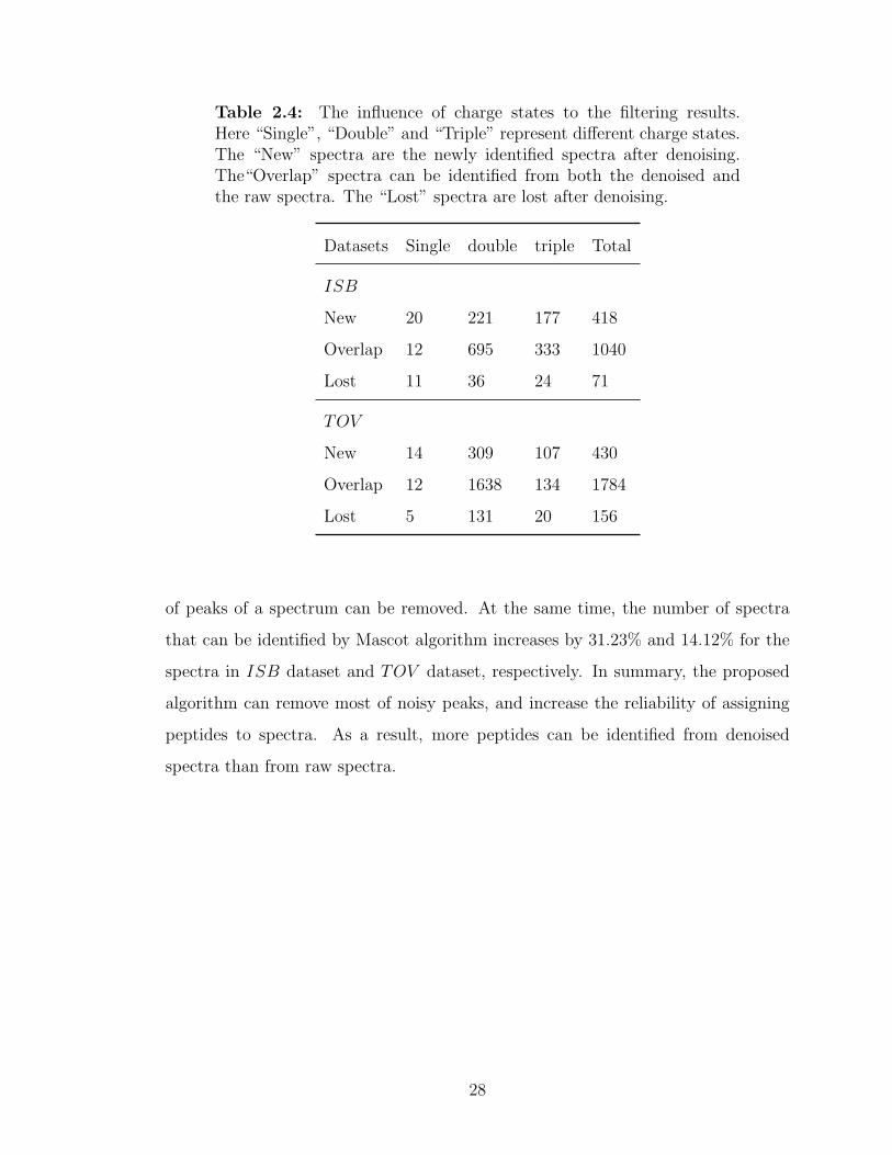
Table 2.4: The influence of charge states to the filtering results.Here “Single”, “Double” and “Triple” represent different charge states.The “New” spectra are the newly identified spectra after denoising.The“Overlap” spectra can be identified from both the denoised andthe raw spectra. The “Lost” spectra are lost after denoising.

Datasets Single double triple Total

ISB

New 20 221 177 418

Overlap 12 695 333 1040

Lost 11 36 24 71

TOV

New 14 309 107 430

Overlap 12 1638 134 1784

Lost 5 131 20 156

of peaks of a spectrum can be removed. At the same time, the number of spectra

that can be identified by Mascot algorithm increases by 31.23% and 14.12% for the

spectra in ISB dataset and TOV dataset, respectively. In summary, the proposed

algorithm can remove most of noisy peaks, and increase the reliability of assigning

peptides to spectra. As a result, more peptides can be identified from denoised

spectra than from raw spectra.

28

Chapter 3

Feature selection for tandem mass spec-

trum quality assessment

3.1 Introduction

For a typical spectrum produced by tandem mass spectrometers, about 80% of peaks

are noise [KL07], most of which can be removed by denoising algorithms. In addition

to the noisy peaks in spectra, many spectra are of poor quality (or called noisy

spectra), e.g., the spectra produced by chemical noise. These poor spectra can’t

be identified by any peptide identification algorithms because they may not contain

enough fragment ions. These poor quality spectra prolong the processing time of

peptide identification algorithms. Moreover, they may cause false identifications

because poor quality spectra may give perfect peptide matches in database search

by pure chance alone [SMF+06]. Therefore, there is a great need to design automatic

spectrum quality assessment algorithms, which can be used to filter out poor quality

spectra before peptide identification.

Automatic spectrum quality assessment has become an important module for

peptide identification from tandem mass spectrum data. Quality assessment is first

used for filtering out poor quality spectra before database search [TEYI01], and is

also used for post-processing of spectra after database search. For example, Nesvizh-

skii et al [NRG+06] used quality assessment to find high quality spectra which had

not been annotated by a first pass database search. These high quality un-annotated

spectra are important because they may be produced by new peptides which are not

in the database, or because they are produced by unexpected modifications on pep-

29

tides. In addition, spectrum quality assessment can also be used for finding false

positives after database search [FMV+06]. Because of the vast number of spectra

produced in a mass spectrometry experiment, automatic quality assessment of tan-

dem mass spectra relies on the application of computational methods.

Machine learning methods, especially supervised learning methods, are widely

used for spectrum quality assessment. Such methods include preliminary rule-

based methods [PKK04, TEYI01], decision tree and random forest [SMF+06], naive

Bayes [FMV+06], logistic regression [WSCC07], Fisher linear discriminative anal-

ysis (FLDA) [WGDP08] and quadratic discriminative analysis (QDA) [BGMY04,

XGB+05]. Recently, as the popularity of support vector machines (SV M) used in

bioinformatics [Nob06], it is also adopted for quality assessment of tandem mass

spectra [BGMY04, NP06]. Regression analysis, such as linear regression [BGMY04],

which gives continues outputs is also considered as an alternative. Recently, Wu et al

[WDP08] prioritized unsupervised learning methods such as mean-shift for quality

assessment [GSM03, CM02]. To use machine learning methods, a fixed-length vector

of real value features is used to represent an original spectrum.

To design an effective automatic spectrum quality assessment algorithm, the

challenging task is to find the relevant features which can best discriminate poor

quality spectra from the ones containing valid peptide information. The overall

accuracy of classifiers can be degraded if important information is not included in

the feature vectors. On the other hand, we should avoid introducing features which

have no or little power to represent the quality of a spectrum. These nearly irrelevant

features may degenerate the performance of classifiers. Besides, it is time and storage

wasting to gather these nearly irrelevant features. In the previous work, the features

used seem to be arbitrary. Some constructed dozens or even more than one hundred

features [BGMY04, FMV+06], while others constructed only two features [NP06].

Little attention has been paid to which features are most relevant to the quality of

a spectrum [FMV+06, SMF+06].

In this chapter, we focus on selecting the relevant features for automatic spec-

trum quality assessment. We first construct most features that can be found in

30

the literature, and then use a sparse logistic regression (SLR) method and a re-

cursive feature elimination based on support vector machines (SV M -RFE) [DR05,

GWBV02, RGE03, TZH07] to select the most relevant features. Experiments are

conducted on two datasets, and the results show the performance of classifiers based

on the selected features is very promising.

3.2 Feature selection

3.2.1 Background

Feature selection in machine learning (or variable selection in statistics) aims at re-

moving irrelevant and redundant features. The irrelevant features do not contribute

to solving classification problems. The redundant features are correlated and thus

can be represented by only one feature. The removing of irrelevant features and

redundant features may improve classifiers’ performance, decrease storage require-

ments and speedup algorithms, save resources in the next round of data collection

and make it easier to interpret the data and visualize the data in lower dimensional

space [GGNZ06, SIL07, RGE03]. Note that in many problems, feature selection does

not always improve classifiers’ performance. In fact, the whole feature set may be

predictive since there is no information loss in them [Mur10, LM07].

Feature selection methods can be classified as unsupervised, semi-supervised and

supervised methods based on whether the label information (dependent variable)

is used for feature selection or not. In the past, most feature selection methods

are supervised, e.g., the widely used penalized feature selection methods which mini-

mize a loss function while imposing a penalty term to shrink some coefficients to zero

[Tib96, HCM+08, MH08]. Feature selection is achieved by removing the features with

zero coefficients. Unsupervised feature selection has gained attention as unlabeled

data have been explored [Gue08, DB04, LM07]. A broad part of unsupervised fea-

ture selection algorithms aim at eliminating redundant features [VGLH06, MMP02].

For unsupervised feature selection methods, there is no label information guiding the

31

feature selection process. For this reason, some assumptions are needed to define the

relevant features. For example, He et al [HCN05] assumes relevant features should

preserve the local structure of the data. While Dash et al [DCSL02] assume that

uniformly distributed features do not provide useful information for clustering. Clus-

tering quality measures are also used to evaluate feature sets [LFJ04, DB04, RD06].

For semi-supervised feature selection, it is only recently used as the popularity of

semi-supervised learning research [ZL07].

Feature selection methods can also be classified as univariate methods if features

are ranked individually and multivariate methods if feature sets are ranked instead

of individual features [HK08]. Typically, univariate methods use hypothesis testing

to rank features. As a result, these methods are very fast but can’t detect redundant

features. Moreover, univariate methods may fail to select the features which are

irrelevant individually but become relevant in the context of others [GGNZ06]. On

the contrary, multivariate methods overcome the shortcoming of univariate methods

by considering the dependance of features. However, as the number of feature subsets

increases exponentially with the number of features. It is not practical to enumerate

all the feature subsets and determine their relevance. Carefully designed methods

are needed to search for the optimal feature subsets.

Feature selection has three aspects: models, search strategies and evaluation

[LM98, LM07]. The three typical models are filter models, wrapper models and

embedded models [LM07]. For a filter model, some criteria are applied for feature

selection, i.e., features are selected by t-test or the correlation coefficients between

features and the label. In contrast to filter models, the wrapper models select fea-

tures by employing specific learning algorithms and optimizing the learning objective

functions. For embedded models, the feature selection process is also the classifier

construction process, i.e., the decision tree algorithm is a typical embedded model

[Bre98]. Most filter models are univariate feature selection which ranks features in-

dividually. Such models are fast and effective, especially for the problems with high

dimensionality and relatively small number of samples. In contrast to filter models,

most wrapper models are multivariate methods which rank sets of features. These

32

models may achieve better results but may take longer time and cause overfitting

problems more easily than filter models. The embedded models may be faster than

wrapper models since they do not need to do cross validations and have higher ca-

pacity than filter models because most embedded models are multivariate methods.

Generally, three types of search strategies are widely used: forward selection,

backward elimination and randomized feature selection [LM07, GGNZ06]. The for-

ward selection methods start with an empty set and progressively add new features.

The widely used Lasso is a type of forward selection method [Tib96]. The backward

elimination methods start with a set of all possible features, and progressively re-

move the most irrelevant features. In contrast to forward selection and background

elimination, the randomized search strategy uses randomization for feature selection.

For different applications, one search strategy may be preferred over the others. The

forward selection and the backward elimination algorithms may select different fea-

ture set, and the latter may be more time consuming than the former algorithm.

Randomization provides an alternative search strategy, and in many situations, the

randomized algorithms are either the simplest or the fastest, and even both [LM07].

There are three criteria widely used to evaluate a feature selection algorithm: the

classification performance, the number of selected features and the stability of the

selected feature set [LM07, GGNZ06, HK08]. One can compare the performances

of classifiers trained with the whole features and the selected features. However, we

should note that feature selection is not confined to improve classifiers’ performance.

For some applications, the number of selected features is more important than the

classifiers’ performance. In addition, domain experts may expect the selected feature

set is stable under different experimental conditions for ease of interpreting the data

[SAdP08]. To compare the performance of different feature selection algorithms, the

evaluation criteria should be computed under the same experimental setting.

In feature selection, the bias produced should be avoided [LZN08, AM02]. The

term “feature selection bias” has two meanings. The first one refers to the per-

formance evaluation bias which is incurred by using the same dataset for feature

selection and for testing the relevance of the selected features. Using this type of

33

biased testing methods, one may get perfect classification as the number of features

increase even on randomly generated datasets [AM02]. The second (less noticed)

feature selection bias refers to the bias incurred by removing features because the

removed features may have useful information. The bias can be avoided by assuming

a statistical model for the joint distribution of features and label [LZN08].

3.2.2 The workflow for selecting the most relevant features

Figure 3.1 shows the workflow of a feature selection method and the verification of

the relevance of the selected features. Firstly, as the intensity of mass spectra is

highly variant, we introduce a local cumulative normalization method to normalize

spectrum intensity. The normalized intensity instead of the original intensity is used

as weight when we construct some features. Secondly, to use machine learning meth-

ods for automatic spectrum quality assessment, each original spectrum is represented

by a feature vector. In the feature construction step, this study collects all possible

features found in the literature to represent a spectrum. Thirdly, we select the most

relevant features out of the constructed features. Fourthly, to test the effectiveness

of the selected features, classifiers are trained using the selected features to predict

the quality of spectra. In the following, we introduce each stage of the workflow.

3.2.3 Local cumulative normalization

Intensity of spectra contains useful information, and can increase the accuracy of

the assignment of peptides to spectra. However, there are no agreed-upon ways

for using intensity information because the intensities of peaks are highly variable

from spectrum to spectrum [BGMY04]. So instead of using the raw intensity of

spectra, intensity is normalized in most cases before any analysis of spectra. For

example, relative intensity normalization divides the raw intensity of each peak by

the intensity of the most abundant peak or the total intensity of all the peaks in a

spectrum. However, relative intensity normalization is sensitive to a few strong peaks

in a spectrum. On the other hand, rank based intensity normalization [BGMY04] is

34

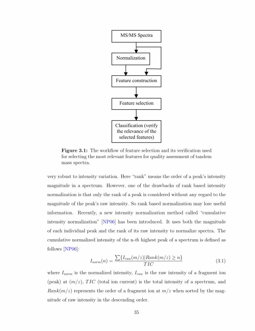
Normalization

Feature construction

Feature selection

Classification (verify the relevance of the

selected features)

MS/MS Spectra

Figure 3.1: The workflow of feature selection and its verification usedfor selecting the most relevant features for quality assessment of tandemmass spectra.

very robust to intensity variation. Here “rank” means the order of a peak’s intensity

magnitude in a spectrum. However, one of the drawbacks of rank based intensity

normalization is that only the rank of a peak is considered without any regard to the

magnitude of the peak’s raw intensity. So rank based normalization may lose useful

information. Recently, a new intensity normalization method called “cumulative

intensity normalization” [NP06] has been introduced. It uses both the magnitude

of each individual peak and the rank of its raw intensity to normalize spectra. The

cumulative normalized intensity of the n-th highest peak of a spectrum is defined as

follows [NP06]:

Inorm(n) =

∑{Iraw(m/z)|Rank(m/z) ≥ n}TIC

(3.1)

where Inorm is the normalized intensity, Iraw is the raw intensity of a fragment ion

(peak) at (m/z), TIC (total ion current) is the total intensity of a spectrum, and

Rank(m/z) represents the order of a fragment ion at m/z when sorted by the mag-

nitude of raw intensity in the descending order.

35

Although the cumulative normalization is a relatively robust method, and it can

increase the number of identified peptide by the SEQUEST search engine [NP06],

it is a “global” method which does not take the effects of mass-to-charge ratio on

peak’s intensity into consideration. For a typical tandem mass spectrum, the peak

intensity is usually higher in the intermediate m/z range, while both the high and

the low m/z ranges are usually composed of peaks with lower intensities [BCG+02].

Thus, only considering the absolute abundance of peaks is not sufficient to normalize

spectra. It would be better to take the difference between regions into consideration.

We introduce a “local cumulative normalization” method here. The local cu-

mulative normalization method calculates the normalized intensity by formula (3.1)

using the ranks of peaks over a window with the width of 56 thompson (Th), instead

of the global rank in [NP06]. Th is the unit of m/z ratio, which is defined as

1Th = 1u

e= 1

Da

e

where u represents the atomic mass unit; Da represents the unit Dalton; and e

represents the elementary charge which is the electric charge unit in the atomic

unit system (http://en.wikipedia.org/wiki/Thomson (unit)). The value of 56 is used

because it is the maximum integer that is less than the minimum mass of the 20

amino acids. This local normalization method is expected to perform better than

the global normalization method in [NP06] because local normalization un-correlates

the mass-to-charge ratio and the intensity, i.e., the normalized intensity of each peak

is determined by its neighbours’ intensity. So peaks at the both ends of a spectrum

have a chance to have the highest intensity of one if their intensities are the local

maxima of the window. This method is similar to the one used by Wong et al

[WSCC07] except that they normalize each peak using a rank based method.

The local accumulative normalization method is used as a pre-processing step

before constructing features in this study. It may also be useful for peptide identi-

fication algorithms to increase performance. Local normalized intensity is used as

weight when we construct features. Using normalized intensity instead of the orig-

inal intensity as weight can significantly decrease the influence of high variance of

36

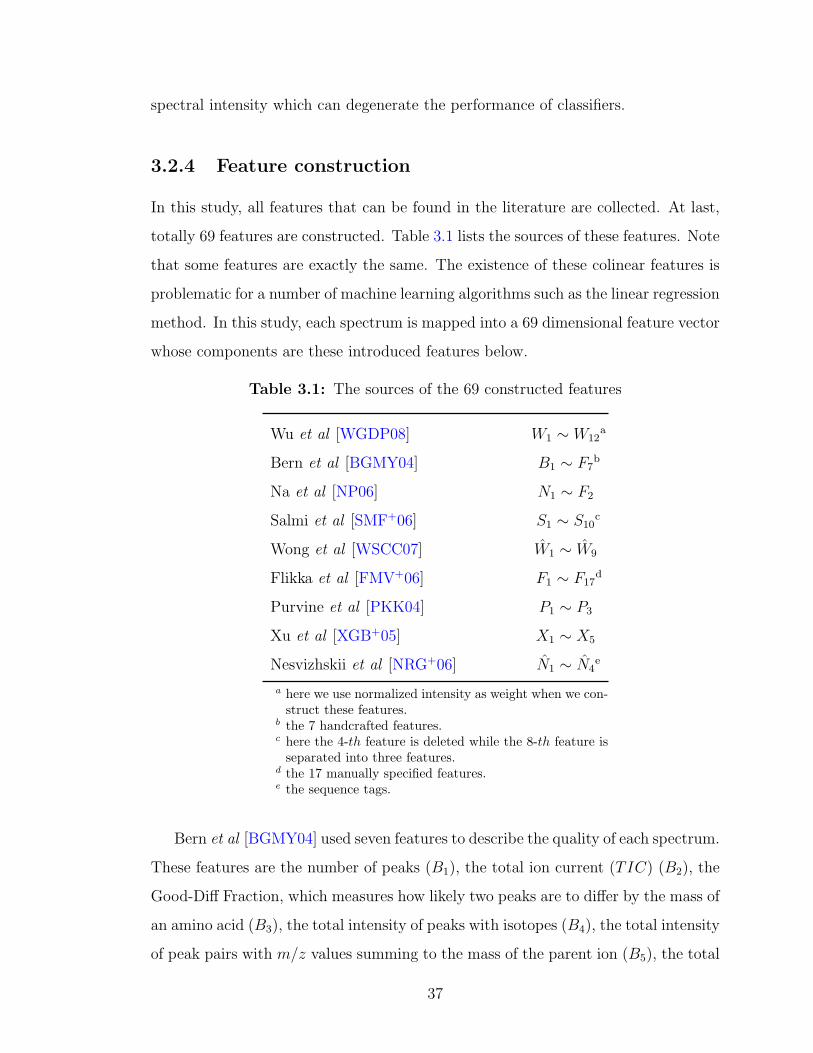
spectral intensity which can degenerate the performance of classifiers.

3.2.4 Feature construction

In this study, all features that can be found in the literature are collected. At last,

totally 69 features are constructed. Table 3.1 lists the sources of these features. Note

that some features are exactly the same. The existence of these colinear features is

problematic for a number of machine learning algorithms such as the linear regression

method. In this study, each spectrum is mapped into a 69 dimensional feature vector

whose components are these introduced features below.

Table 3.1: The sources of the 69 constructed features

Wu et al [WGDP08] W1 ∼ W12a

Bern et al [BGMY04] B1 ∼ F7b

Na et al [NP06] N1 ∼ F2

Salmi et al [SMF+06] S1 ∼ S10c

Wong et al [WSCC07] W1 ∼ W9

Flikka et al [FMV+06] F1 ∼ F17d

Purvine et al [PKK04] P1 ∼ P3

Xu et al [XGB+05] X1 ∼ X5

Nesvizhskii et al [NRG+06] N1 ∼ N4e

a here we use normalized intensity as weight when we con-struct these features.

b the 7 handcrafted features.c here the 4-th feature is deleted while the 8-th feature is

separated into three features.d the 17 manually specified features.e the sequence tags.

Bern et al [BGMY04] used seven features to describe the quality of each spectrum.

These features are the number of peaks (B1), the total ion current (TIC) (B2), the

Good-Diff Fraction, which measures how likely two peaks are to differ by the mass of

an amino acid (B3), the total intensity of peaks with isotopes (B4), the total intensity

of peak pairs with m/z values summing to the mass of the parent ion (B5), the total

37

intensity of pairs of peaks with m/z values differing by 18 Da (B6), and the intensity

balance (B7). Note that in the same paper [BGMY04], Bern et al use another 186

features as inputs of SV M , but the SV M does not perform well enough. Therefore,

this study does not consider these 186 features.

Purvine et al [PKK04] proposed three features to describe the quality of each

spectrum. These features are charge state (P1), TIC (P2), and signal-to-noise esti-

mation (P3).

Xu et al [XGB+05] used four variables derived from five features of spectra to

construct a quadratic discriminative function. The five features are the number of

peaks larger than 5% of base peak intensity (X1), the number of peaks larger than

3% (X2) and 2% (X3) of TIC, the average peak distance along m/z for the peaks

larger than 2% of TIC (X4) and within 1.0 ∼ 1.5% of TIC (X5).

Na et al [NP06] used only two features to describe the quality of a spectrum.

The first feature is xrea (N1), which is computed after normalizing spectra by the

cumulative normalization method [NP06]. The second feature is Good-Diff Fraction

(N2).

Flikka et al [FMV+06] used 17 manually specified features, all the between-peak

mass difference (deltas), and all possible m/z values to describe the quality of a

spectrum. However, as stated in [FMV+06], the between-peak mass difference and

all possible m/z values are not very discriminative compared to the 17 manually

specified features. So we only consider the 17 manually specified features in this

study. These features are the number of peaks (F1), the number of significant peaks

(F2) (peaks with relative intensity greater than 0.1), the number of significant peaks

divided by precursor mass (F3), the average delta mass in a spectrum (F4), the stan-

dard deviation of delta mass values (F5), the charge of precursor ion (F6), the mass of

uncharged precursor (F7), the m/z value of a precursor in a parent spectrum (F8), the

relative intensity of the precursor in the fragment spectrum (F9), the intensity differ-

ence between the top two peaks (F10), the (number of peaks)/(max mz −min mz)

(F11), the number of peaks accounting for 5% of the total intensity (F12), the average

of relative peak intensities (F13), the standard deviation of relative peak intensities

38

(F14), the total raw intensities for significant peaks (F15), the total relative intensities

for significant peaks (F16), the total relative intensity of complementary pairs (F17).

Salmi et al [SMF+06] used nine features to describe the quality of a spectrum.

Some features are specific to their spectra such as the total intensity of peaks result-

ing from the ICAT reagent. Based on these nine features, for general spectra, we

construct ten slightly different features. These features are: the average intensity of

the peaks in the spectrum (S1), the standard deviation of the peak intensities in the

spectrum (S2), the total intensity of exceptionally high peaks in the spectrum (S3),

the presence of immonium ions in the spectrum (S4), the total intensity of fragment

y1 ion peak (S5), the total intensity of the precursor peak (S6), the total intensity of

yn−2 ion (S7), the total intensity of b2 ion (S8), the total intensity of bn−1 ion (S9),

and a score based on mass-ladder (S10).

According to the properties of theoretical spectra and the principle of peptide

fragmentation by tandem mass spectrometers, Wu et al [WGDP08] used twelve

features to describe the quality of a spectrum. These features can be classified into

four categories: the first three features (W1,W2,W3) are the number of peaks with

the difference of the mass of one of the 20 amino acids, (W4,W5,W6) are the number

of peaks with m/z values summing to the mass of their parent ion, (W7,W8,W9)

are the total number of peaks with m/z values differing by the mass of a water

molecule or an ammonia molecule, (W10,W11,W12) are the total number of peaks

with m/z values differing by the mass of a CO group or an NH group. Here we

use normalized intensity as weight when we construct these features although the

intensity was ignored in [WGDP08].

Recently, seven out of nine features were used to construct a logistic regression

model to predict the quality of tandem mass spectra by Wong et al [WSCC07].

These features are the number of peaks in a spectrum (W1), normalized TIC (W2)

(because we do not know which spectra were produced by a specific run, we just use

TIC instead), GoodSegs (W3), the ratio of the number of peaks which have relative

intensities greater than 1% of the total intensity to the total number of peaks in a

spectrum (W4), the ratio of the number of peaks that have relative intensities greater

39

than 20% of total intensity to the total number of peaks in a spectrum (W5), pairs

of peaks whose m/z values add together to give the m/z of the parent (W6), the

presence of isotope peaks associated with an inferred b or y ion (W7), the presence of

water loss peaks associated with an inferred b or y ion (W8), the ninth feature (W9)

which quantifies evidence for inferred b or y pairs separated by amino acid masses.

Nesvizhskii et al constructed 40 features to describe the quality of a spectrum.

However, most features are considered in the previous papers. We only construct

four features which are not considered by the previous papers. These features are

the length of the longest sequence tag that can be extracted from a spectrum (N1),

the average length of all extracted sequence tags (N2), the number of sequence tag

of length one (N3) and a derived version of N3 computed using the peak intensities

as weight factors (N4).

At this point, we have introduced 69 features found in the literature to describe

the quality of a spectrum. In this study, each spectrum is mapped into a 69 dimen-

sional feature vector whose components are these introduced features. As discussed

earlier, some of these features may be very relevant to the quality of tandem mass

spectra, and others may be not. In the next subsections, we introduce a sparse lo-

gistic regression model and a recursive feature elimination based on support vector

machines (SV M -RFE) to select the most relevant features from those 69 introduced

features.

3.2.5 Feature selection using sparse logistic regression

Logistic regression

Consider a training spectral dataset

X = {xi, yi}Ni=1, i = 1, . . . , N

xi ∈ RD, yi ∈ {0, 1}

where xi represents the i-th sample, a D-dimensional feature vector; yi is the class

label; and N is the number of training spectra. The logistic regression (LR) meth-

40

ods attempt to model the posterior probabilities of class memberships via logistic

function of x.

p(y = 1|x,w, w0) = σ(wTx + w0) (3.2)

where σ(η) = 11+e−η is the logistic function or sigmoid function, w0 is the intercept,

and w = (w1, . . . , wD) collects the coefficients.

More formally, the logistic regression model uses a Bernoulli model for the like-

lihood [Mur10, Alp04]. Therefore the likelihood is given by

p(y|x,w, w0) = σ(η)y(1− σ(η))1−y (3.3)

where η = wTx + w0.

Assume that X consists of N independent and identically distributed samples

from a Bernoulli distribution, the negative log-likelihood function is given by

J(w, w0) = −N∑

i=1

log p(yi|xi,w, w0) (3.4)

= −N∑

i=1

[yi log(σ(ηi) + (1− yi) log(1− σ(ηi))]

This negative log-likelihood function can be efficiently minimized by iterative gradient-

based methods.

Sparse logistic regression

The coefficients in Equation 3.4 corresponding to irrelevant features should be zeros

and thus w is a sparse vector. However, the resulting model obtained by minimizing

the log-likelihood function Equation 3.4 may not be sparse. To get the sparse rep-

resentation, an L1-regularization term is added to Equation 3.4 as a penalty. Thus

we get the following L1-regularized objective function:

J(w, w0, λ) = −N∑

i=1

log p(yi|xi,w, w0) + λ||w||1 (3.5)

where λ is a positive scalar regularization parameter which controls the sparsity of the

resulting model, ||w||1 =∑

i |wi| is the 1-norm. The L1 regularization corresponds

41

to a Laplace prior, and this is a binary classification equivalence of Lasso [Tib96,

Mur10]. The regularization parameter λ can be selected by cross validation or from

a Bayesian approach [CT06]. Note that all components of w are penalized equally

by λ, so it is important that all components of w are on the same scale. Therefore

each feature is standardized with the mean of zero and the variance of one in this

study.

To find w and wo which minimizes (3.5) is an active research area. There exist a

large number of algorithms. Since the objective function (3.5) is convex, and the L1

norm is not differentiable, one can use generic methods for solving nondifferentiable

convex problems. Recently, an efficient interior-point method was proposed [KKB07].

This algorithm takes truncated Newton steps and uses preconditioned conjugated

gradient iterations. It can also produce high-precision solutions. Thus this algorithm

is adopted as the sparse logistic regression solver.

3.2.6 Feature selection using SVM-RFE

Support vector machine

Support vector machines (SV M) were widely used years ago in statistical learning

for solving classification and regression problems. Now it is becoming popular in a

variety of biological applications [Nob06]. Here we briefly introduce SV M for the

two-class classification problem which our problems belong to. A general discussion

of SV M can be found in [Bis06, Vap98, Vap00, CST00, SS02].

For an SV M classifier, suppose that a training set composed of N spectral sam-

ples xi ∈ RD with corresponding labels yi ∈ {−1, 1} where i = 1, . . . , N . We assume

that yi ∈ {−1, 1} instead of {0, 1} as in logistic regression for the ease of discussion.

In fact, we can convert {−1, 1} back to {0, 1} easily by a linear transformation.

If the original samples are not linear separable, the samples may become linear

separable by introducing some nonlinear mapping to map a sample xi to Φ(xi),

where Φ(x) is a feature mapping [GS00], e.g.,

Φ(x) = (x21,√

2x1x2,x22).

42

A unique optimal separating hyperplane (OSH) [HS01]

f(x) = wT Φ(x) + b

can be constructed by maximizing the margin–the distance between the hyperplane

and the nearest data points of each class. Maximizing the margin is equivalent to

min1

2‖w‖2

subjecting to the constraint of

yi(wT Φ(x) + b) ≥ 1.

Note that we do not need to compute Φ(x) for each training data point x to find w

and b of the optimal hyperplane. Instead, for some nonlinear mappings, we can find

a kernel which satisfies

k(xi,xj) = Φ(xi)T Φ(xj)

and the problem of finding the optimal hyperplane can be done by only dot product

computation in the feature space where the original samples are mapped to. There-

fore, the dot product evaluation in feature space can be simplified to kernel function

evaluation in the input space. This simplification is called the “kernel” technique

[ABR64, SS02].

It is possible and desirable to find a hyperplane with large margin by allowing

some samples been misclassified. This technique is called “soft margin” and is nec-

essary in practice. For example, there may not exist a hyperplane which perfectly

separates the data in feature space, or the margin may be too narrow. In these

circumstances, the soft margin classifier is necessary to find a maximum margin

classifier without causing overfitting.

To implement the soft margin classifier, a sample is penalized by

ζi = |yi − (wT Φ(x) + b)|

if the sample is misclassified or it is inside the margin boundary. The OSH [HS01]

is then regarded as the solution of the optimization problem

arg minw,b

C

N∑i=1

ζi +1

2‖ w ‖2

43

under constraints

yif(xi) ≥ 1− ζi

where C > 0 is a regularization parameter which controls the trade-off between

the complexity of margin and misclassification error. The problem is a constrained

optimization problem and can be solved by the use of Lagrange multipliers. The

corresponding objective function is given in the next subsection. From the above

discussion, we can see a support vector machine is essentially a kernelized maximum

margin hyperplane classifier with soft margin.

SVM-RFE algorithm

The recursive feature elimination based on support vector machine algorithm (SV M -

FRE) is one of the backward elimination methods widely used for many problems

[GWBV02, HS01, ZLS+06], but it has not been used for quality assessment of tandem

mass spectra yet. This study will apply the SV M -FRE to select a set of the most

relevant features for the purpose of quality assessment of spectra. Consider a set

of N tandem mass spectra with their quality labels “-1” (for poor quality) or “1”

(for high quality). Let D be the dimension of feature vectors. For spectrum i in

the spectral dataset, let xi be a D-dimensional feature vector whose components are

described in the previous subsection, and yi be its quality label. The SV M -RFE

recursively does the following steps.

Step 1. Train an SV M by solving the following quadratic optimization problem

Minimize : L(a) = −N∑

i=1

ai +1

2

N∑i=1

N∑j=1

aiajyiyjk(xi,xj) (3.6)

Subject to :N∑

i=1

aiyi = 0, and 0 ≤ ai ≤ C, (i = 1, 2, . . . , N)

where a = {a1, a2, . . . , aN} is a parameter vector to be found, C is a regulariza-

tion parameter which controls the trade-off between misclassification errors and

model complexity, and k(xi,xj) is a kernel function. The simplest kernel function

is k(xi,xj) = xTi xj, which is the linear kernel. Commonly used nonlinear kernel

functions are radial basis functions, which are defined as k(xi,xj) = r(‖xi − xj‖2)

44

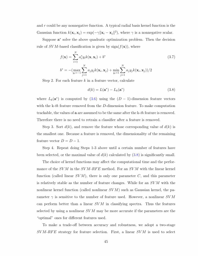
and r could be any nonnegative function. A typical radial basis kernel function is the

Gaussian function k(xi,xj) = exp(−γ‖xi − xj‖2), where γ is a nonnegative scalar.

Suppose a∗ solve the above quadratic optimization problem. Then the decision

rule of SV M -based classification is given by sign(f(x)), where

f(x) =N∑

i=1

a∗i yik(x,xi) + b∗ (3.7)

b∗ = −(maxyi=−1

N∑j=1

ajyjk(xi,xj) + minyi=1

N∑j=1

ajyjk(xi,xj))/2

Step 2. For each feature k in a feature vector, calculate

d(k) = L(a∗)− Lk(a∗) (3.8)

where Lk(a∗) is computed by (3.6) using the (D − 1)-dimension feature vectors

with the k-th feature removed from the D-dimension feature. To make computation

trackable, the values of a are assumed to be the same after the k-th feature is removed.

Therefore there is no need to retrain a classifier after a feature is removed.

Step 3. Sort d(k), and remove the feature whose corresponding value of d(k) is

the smallest one. Because a feature is removed, the dimensionality of the remaining

feature vector D = D − 1.

Step 4. Repeat doing Steps 1-3 above until a certain number of features have

been selected, or the maximal value of d(k) calculated by (3.8) is significantly small.

The choice of kernel functions may affect the computational time and the perfor-

mance of the SV M in the SV M -RFE method. For an SV M with the linear kernel

function (called linear SV M), there is only one parameter C, and this parameter

is relatively stable as the number of feature changes. While for an SV M with the

nonlinear kernel function (called nonlinear SV M) such as Gaussian kernel, the pa-

rameter γ is sensitive to the number of feature used. However, a nonlinear SV M

can perform better than a linear SV M in classifying spectra. Thus the features

selected by using a nonlinear SV M may be more accurate if the parameters are the

“optimal” ones for different features used.

To make a trade-off between accuracy and robustness, we adopt a two-stage

SV M -RFE strategy for feature selection. First, a linear SV M is used to select

45

D (D = 15 in this study) most relevant features. Here the value of 15 for D is

chosen according to the number of support vectors obtained after training an SV M

classifier. Generally, when the number of support vectors becomes very large, this

phenomena may indicate that overfitting is occurred or we have removed relevant

features. Secondly, a nonlinear SV M with Gaussian kernel is used for ranking the

D most relevant features.

Unlike the sparse logistic regression, the SV M -RFE algorithm may select redun-

dant features. For the 69 constructed features, some of them are exactly the same.

For this reason, we only retain one of the features which are exactly the same. After

the process of removing the redundant features, only 61 features are left. We use the

proposed two-stage SV M -RFE algorithm to select the most relevant features out

of the 61 features.

The LIBSVM [CL01] is adopted as the SV M solver in this study. The hyper-

parameters of SV Ms are selected by a five-cross validation on the training data. For

linear SV M , the parameter C is set to 0.08; for Gaussian kernel, the parameter C

is set to 100, and γ is set to 0.08. For SV M classifiers, large C and γ may cause

overfitting.

3.3 Results and discussion

3.3.1 Experimental datasets

This study employs two tandem mass spectral datasets: ISB dataset and TOV

dataset to investigate the performance of the proposed method. The following is a

brief description of these datasets.

(1) ISB dataset. This dataset consisting of 22 LC/MS/MS runs was produced

by Institute of System Biology (ISB) from 18 control mixture proteins [KPN+02].

Tandem mass spectra in this dataset were searched using SEQUEST against a human

protein database appended with sequences of the 18 control mixture proteins. This

analysis produced 18, 496 assignments to doubly charged spectra, 18, 044 to triply

46

charged spectra, and 504 to singly charged spectra. After manual validation, 1656

peptide assignments to doubly charged spectra, 984 to triply charged spectra, and

132 to singly charged spectra were determined to be correct. These data were also

analyzed by InsPecT which annotated another 820 possibly modified (mutated)

peptides [TSF+05]. All these 3592 spectra are labeled as “high” quality, and all the

other spectra in the dataset are labeled as “poor” quality in this study.

(2) TOV dataset. The data in TOV dataset consists of 22, 576 ion trap spectra.

These MS/MS spectra were searched against a subset of the Uniref100 database (re-

lease 1.2, http://www.uniprot.org) containing 44, 278 human protein sequences using

SEQUEST. This analysis produced 10, 714 assignments to doubly charged spectra,

9732 to triply charged spectra, and 2430 to singly charged spectra. After validated

by PeptideProphet [KNKA02], 1898 peptide assignments to doubly charged spectra,

261 to triply charged spectra, and 38 to singly charged spectra were determined to

be correct (PeptideProphet scores equal or greater than 0.9). All these 2197 spectra

are labeled as “high” quality in this study. All the other spectra in the dataset are

labeled as “poor” quality.

3.3.2 Training and performance evaluation

The effectiveness of the proposed feature selection method is evaluated by comparing

the performance of the classifiers trained with different set of features. We first divide

the ISB dataset into two equal size subsets: one for feature selection and classifier

training, the other for classifier testing. Each subset has the same number of high

quality spectra and poor quality spectra. It is expected that the most relevant

features selected based on the ISB dataset can be applicable to other datasets to

train superior classifiers. To do this we also divide the TOV dataset into two equal

size subsets as for the ISB dataset. One subset is used to train classifiers with the

features selected based on the ISB dataset, while the other subset is used to evaluate

the performance of the classifiers.

For the evaluation of the performance of the trained classifiers, we reported true

positive rates (TPR, the fraction of positives corrected classified as positives) and

47

false positive rates (FPR, the fraction of negatives misclassified as positives). We

also reported receiver operating characteristic (ROC) curves [Faw04], which are a

plot of TPR as a function of FPR. The ROC curve is very useful to view a classifier’s

performance and tune a classifier to have a fixed TPR or true negative rate (TNR,

the fraction of negatives correctly classified as negatives and TNR = 1 − FPR).

For the unbalanced data which have different number of positives and negatives, to

tune a classifier is very important. The area under the curve (AUC) was used for

comparing classification results. The AUC is 1 for perfect classification and 0.5 just

the same as random guess.

3.3.3 Feature selected by SLR and the classification results

To select the truly highly relevant features and remove the false positives, we con-

struct several subsets of the training data, and run L1-regularized logistic regression

on the subsets. The final selected features are the intersect of the multiple runs.

To do this, a number of training subsets are constructed from the training data for

feature selection. These training subsets can be constructed by bootstrap resampling

[Efr79, HMM+05]. However, for tandem mass spectrum data, the numbers of high

quality and poor quality spectra are highly biased. For this reason, we first extract

the high quality spectra from the training subset, then we randomly draw the same

number of poor quality spectra from the training subset. This processing is repeated

25 times, and we get 25 subsets for feature selection.

Figure 3.2 shows the selection frequency (top panel) and the absolute values of

the mean weights of the 69 features (bottom panel). The more frequently the features

are selected, the more likely the features are highly relevant because these features

are not likely selected by chance. In addition, the features with large weights are

more likely to be relevant features than those with small weights because the features

with large weights will contribute significantly to compute the posterior probability

in logistic models. From Figure 3.2, we can see that the more frequently selected

features also have larger weights than the less selected features in general. Therefore,

in this study the features occur 80% of times (i.e., 20 times) are selected. By using

48

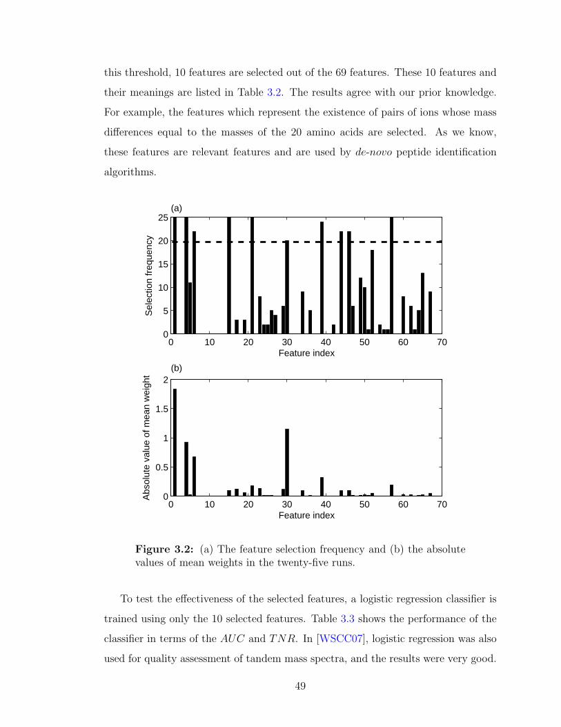
this threshold, 10 features are selected out of the 69 features. These 10 features and

their meanings are listed in Table 3.2. The results agree with our prior knowledge.

For example, the features which represent the existence of pairs of ions whose mass

differences equal to the masses of the 20 amino acids are selected. As we know,

these features are relevant features and are used by de-novo peptide identification

algorithms.

0 10 20 30 40 50 60 700

5

10

15

20

25

Feature index

Sel

ectio

n fr

eque

ncy

(a)

0 10 20 30 40 50 60 700

0.5

1

1.5

2

Feature index

Abs

olut

e va

lue

of m

ean

wei

ght

(b)

Figure 3.2: (a) The feature selection frequency and (b) the absolutevalues of mean weights in the twenty-five runs.

To test the effectiveness of the selected features, a logistic regression classifier is

trained using only the 10 selected features. Table 3.3 shows the performance of the

classifier in terms of the AUC and TNR. In [WSCC07], logistic regression was also

used for quality assessment of tandem mass spectra, and the results were very good.

49

Table 3.2: The selected features by the SLR model and the meaningsof the selected features.

Index Feature meanings

W1 Amino acid distance (singly charged)

W4 Complementary ions (singly charged)

W6 Complementary ions (multiply charged)

B3 Good-Diff Fraction

N1 xrea

S9 Total intensity of bn−1 ion

W8 Water loss

F4 Average delta mass in spectra

F6 Charge of precursor ions

F17 Total intensity of complementary pairs

In their study, logistic regression classifier was used to classify tandem mass spectra

based on nine features. In this study, we also construct their nine features, and

construct a logistic regression model for quality assessment of tandem mass spectra.

The results are also shown in Table 3.3.

Table 3.3: Compare the overall classification results using differentfeatures selected by the SLR model in terms of AUC and TNR at afixed true positive rate of 90%.

Features ISB TOV

AUC TNR AUC TNR

Wong’s 0.88 73.79% 0.90 76.45%

Selected 0.93 80.48% 0.95 85.06%

From the classification results shown in Table 3.3, the performance of classifiers

based on the selected ten features is better than that based on the nine features

constructed in [WSCC07]. The results indicate the proposed sparse logistic regression

method can successfully select the highly relevant features.

50

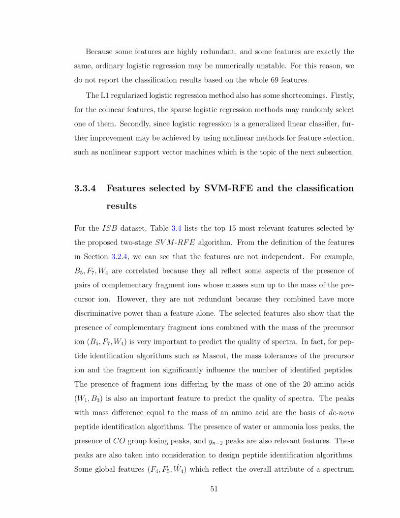
Because some features are highly redundant, and some features are exactly the

same, ordinary logistic regression may be numerically unstable. For this reason, we

do not report the classification results based on the whole 69 features.

The L1 regularized logistic regression method also has some shortcomings. Firstly,

for the colinear features, the sparse logistic regression methods may randomly select

one of them. Secondly, since logistic regression is a generalized linear classifier, fur-

ther improvement may be achieved by using nonlinear methods for feature selection,

such as nonlinear support vector machines which is the topic of the next subsection.

3.3.4 Features selected by SVM-RFE and the classification

results

For the ISB dataset, Table 3.4 lists the top 15 most relevant features selected by

the proposed two-stage SV M -RFE algorithm. From the definition of the features

in Section 3.2.4, we can see that the features are not independent. For example,

B5, F7,W4 are correlated because they all reflect some aspects of the presence of

pairs of complementary fragment ions whose masses sum up to the mass of the pre-

cursor ion. However, they are not redundant because they combined have more

discriminative power than a feature alone. The selected features also show that the

presence of complementary fragment ions combined with the mass of the precursor

ion (B5, F7,W4) is very important to predict the quality of spectra. In fact, for pep-

tide identification algorithms such as Mascot, the mass tolerances of the precursor

ion and the fragment ion significantly influence the number of identified peptides.

The presence of fragment ions differing by the mass of one of the 20 amino acids

(W1, B3) is also an important feature to predict the quality of spectra. The peaks

with mass difference equal to the mass of an amino acid are the basis of de-novo

peptide identification algorithms. The presence of water or ammonia loss peaks, the

presence of CO group losing peaks, and yn−2 peaks are also relevant features. These

peaks are also taken into consideration to design peptide identification algorithms.

Some global features (F4, F5, W4) which reflect the overall attribute of a spectrum

51

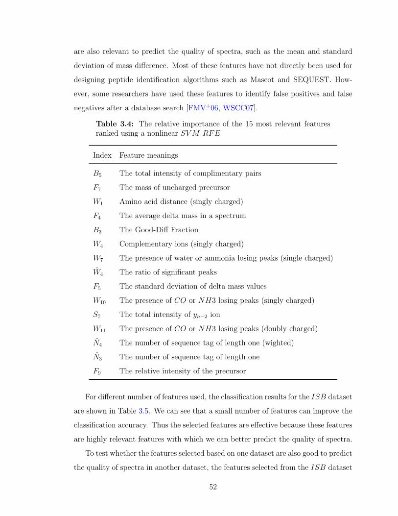
are also relevant to predict the quality of spectra, such as the mean and standard

deviation of mass difference. Most of these features have not directly been used for

designing peptide identification algorithms such as Mascot and SEQUEST. How-

ever, some researchers have used these features to identify false positives and false

negatives after a database search [FMV+06, WSCC07].

Table 3.4: The relative importance of the 15 most relevant featuresranked using a nonlinear SV M -RFE

Index Feature meanings

B5 The total intensity of complimentary pairs

F7 The mass of uncharged precursor

W1 Amino acid distance (singly charged)

F4 The average delta mass in a spectrum

B3 The Good-Diff Fraction

W4 Complementary ions (singly charged)

W7 The presence of water or ammonia losing peaks (single charged)

W4 The ratio of significant peaks

F5 The standard deviation of delta mass values

W10 The presence of CO or NH3 losing peaks (singly charged)

S7 The total intensity of yn−2 ion

W11 The presence of CO or NH3 losing peaks (doubly charged)

N4 The number of sequence tag of length one (wighted)

N3 The number of sequence tag of length one

F9 The relative intensity of the precursor

For different number of features used, the classification results for the ISB dataset

are shown in Table 3.5. We can see that a small number of features can improve the

classification accuracy. Thus the selected features are effective because these features

are highly relevant features with which we can better predict the quality of spectra.

To test whether the features selected based on one dataset are also good to predict

the quality of spectra in another dataset, the features selected from the ISB dataset

52

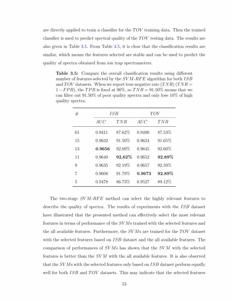
are directly applied to train a classifier for the TOV training data. Then the trained

classifier is used to predict spectral quality of the TOV testing data. The results are

also given in Table 3.5. From Table 3.5, it is clear that the classification results are

similar, which means the features selected are stable and can be used to predict the

quality of spectra obtained from ion trap spectrameters.

Table 3.5: Compare the overall classification results using differentnumber of features selected by the SV M -RFE algorithm for both ISBand TOV datasets. When we report true negative rate (TNR) (TNR =1−FPR), the TPR is fixed at 90%, so TNR = 91.50% means that wecan filter out 91.50% of poor quality spectra and only lose 10% of highquality spectra.

# ISB TOV

AUC TNR AUC TNR

61 0.9411 87.62% 0.9490 87.53%

15 0.9632 91.50% 0.9624 91.65%

13 0.9656 92.09% 0.9645 92.60%

11 0.9640 92.62% 0.9652 92.89%

9 0.9635 92.19% 0.9657 92.59%

7 0.9608 91.79% 0.9673 92.89%

5 0.9478 86.73% 0.9527 89.12%

The two-stage SV M -RFE method can select the highly relevant features to

describe the quality of spectra. The results of experiments with the ISB dataset

have illustrated that the presented method can effectively select the most relevant

features in terms of performance of the SV Ms trained with the selected features and

the all available features. Furthermore, the SV Ms are trained for the TOV dataset

with the selected features based on ISB dataset and the all available features. The

comparison of performances of SV Ms has shown that the SV M with the selected

features is better than the SV M with the all available features. It is also observed

that the SV Ms with the selected features only based on ISB dataset perform equally

well for both ISB and TOV datasets. This may indicate that the selected features

53

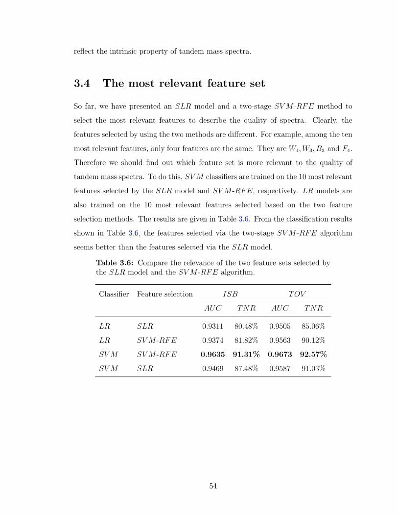
reflect the intrinsic property of tandem mass spectra.

3.4 The most relevant feature set

So far, we have presented an SLR model and a two-stage SV M -RFE method to

select the most relevant features to describe the quality of spectra. Clearly, the

features selected by using the two methods are different. For example, among the ten

most relevant features, only four features are the same. They are W1,W3, B3 and F4.

Therefore we should find out which feature set is more relevant to the quality of

tandem mass spectra. To do this, SV M classifiers are trained on the 10 most relevant

features selected by the SLR model and SV M -RFE, respectively. LR models are

also trained on the 10 most relevant features selected based on the two feature

selection methods. The results are given in Table 3.6. From the classification results

shown in Table 3.6, the features selected via the two-stage SV M -RFE algorithm

seems better than the features selected via the SLR model.

Table 3.6: Compare the relevance of the two feature sets selected bythe SLR model and the SV M -RFE algorithm.

Classifier Feature selection ISB TOV

AUC TNR AUC TNR

LR SLR 0.9311 80.48% 0.9505 85.06%

LR SV M -RFE 0.9374 81.82% 0.9563 90.12%

SV M SV M -RFE 0.9635 91.31% 0.9673 92.57%

SV M SLR 0.9469 87.48% 0.9587 91.03%

54

Chapter 4

Clustering analysis for mass spectrum

quality assessment

4.1 Introduction

In the past, several supervised machine learning algorithms have been proposed to

assess the quality of tandem mass spectra. For supervised machine learning, a labeled

training dataset is needed to train a classifier, and the trained classifier is used to

classify spectra as high quality or poor quality. Ideally, the spectra of the training

set should be identified by several peptide identification algorithms and manually

validated, i.e., the set should be correctly labeled without or with very few falsely

labeled spectra. However, such spectral data sets are hard to obtain in most cases.

Worse still, tandem mass spectrometers may produce different spectra even for the

same peptide under different experimental conditions. Therefore, the training and

testing spectra may not come from the same probability distribution and the trained

classifier may fail to discriminate poor quality spectra from high quality ones. The

performance of classifiers can be improved by training a specific classifier for each

experiment. On the other hand, clustering algorithms, which do not need a training

set, may be alterative choices for the quality assessment of tandem mass spectra.

In this chapter, we use clustering algorithms to cluster the experimental spectra

without using any prior information about the spectral dataset from search engines.

The remainder of this chapter is organized as follows. Section 4.2 introduces the

model based clustering algorithm. In Section 4.3, the ISB and the TOV datasets

are used to investigate the performance of the algorithm. The experimental results

55

show the model based clustering algorithm can remove about 57.64% and 66.36%

of poor quality spectra while losing only 10% of high quality spectra for the two

tandem mass spectral datasets: ISB and TOV dataset, respectively.

4.2 Clustering analysis

4.2.1 Background

Contrast to supervised learning methods, the unsupervised learning methods do

not need a labeled training set. Several types of unsupervised learning methods

are widely used. The first type of methods is density estimation which estimates the

underlying probability density function P (X) of a given dataset X. The second type

of methods is dimension reduction methods such as principle component analysis,

independent component analysis, and multidimensional scaling. The third type of

methods is clustering [Fuk90, HTF01, Mur10].

Clustering is the assignment of data to different groups so that data in the same

group are more similar than those in different groups [HTF01, JMF99]. Clustering

is a difficult problem since no prior information about the data is given. Therefore

we need to make some assumptions to solve the clustering problems. For example,

the k -means algorithm assumes data can be grouped into spherical and nearly the

same size clusters [Mac67]. The model based clustering methods assume that data

are generated from a predefined statistical model. Since different definitions of the

clustering can result in different clusters, there is no single best clustering algorithm.

Accordingly, the definition of clustering is at the heart of clustering algorithm design

[Web02, Fuk90].

According to the different definitions of clustering, the existing clustering meth-

ods can be classified as combinatorial, model based and mode seeking algorithms

[HTF01, JMF99]. Combinatorial algorithms do not assume a probability distribu-

tion on the data, and samples are assigned to clusters by optimizing an objective

function [Mac67, SM00, FD07]. Contrary to combinatorial methods, the statistical

56

model based methods assume samples are independent and identically distributed

from a predefined probability density function such as mixture of Gaussian distribu-

tions. After inferring the unknown parameters, clustering is achieved by assigning

samples to different Gaussian components [Bil98, DLR77]. When the assumed prob-

abilistic distribution is correct, the model based algorithm may achieve good clus-

tering results. The mode seeking methods take a nonparametric approach to find

the modes of the probability density function of data, and a sample is assigned to its

nearest mode [HTF01, CM02]. The mode seeking methods may be good choices if

the structure of data is very complex and can’t be modeled by a simple parametric

probability distribution.

The existing clustering methods can also be classified as hierarchical and parti-

tional clustering. For hierarchical clustering, a hierarchical tree can be constructed

in two ways: bottom-up and top-down. At the beginning, the bottom-up hierarchi-

cal clustering method views a single point as a group. The two most similar groups

are merged successively until all the data are merged into a single cluster [Web02].

Alternatively, the top-down hierarchal clustering method successively splits groups

until each group has only one single point. Hierarchical clustering is pretty useful

when the data can be described by a tree. However, the hierarchical tree is not sta-

ble, a small change in data may change the tree completely. Partitional clustering,

on the other hand, divides the data into disjoint clusters. Thus the final clusters are

flat. In the following, we will use a partitional clustering algorithm – a model based

clustering algorithm for the quality assessment of tandem mass spectra. This algo-

rithm is a parametrical method since it assumes a predefined probability distribution

of spectral feature data.

4.2.2 Model based clustering for quality assessment

After exploratory data analysis and from previous research [BGMY04, WGDP08],

the distribution of high quality spectra and poor quality spectra can be modeled by

57

a mixture of Gaussian distributions:

p(x) =K∑

k=1

πkN (x|µk, Σk) (4.1)

where K is the number of mixture components and here K = 2; one component

corresponds to high quality spectra while the other component corresponds to poor

quality spectra. πk is the mixture coefficient. N (x|µk, Σk) is a Gaussian density

function with its mean of µk and covariance matrix of Σk, and x is a feature vector.

For this study, we use the EM (expectation maximization) algorithm (see below) to

estimate the parameters of the Gaussian mixture model [Bil98].

To use the EM algorithm for parameter estimation, we need to provide the initial

guess of the parameters. Here the k -means algorithm is used to initialize the EM

algorithm [Mac67, AV07].

K -means

K -means (also known as C-means) is a kind of combinational algorithm. For given

unlabeled feature vectors xn ∈ RD (n = 1, . . . , N), we want to partition the N

data points into K clusters. The exhaustive search is not practical because there

are approximately NK

K!possible partitions. Alteratively, an objective function can

be defined to measure the quality of a partition so the partition problem can be

formulated as minimizing the objective function. To define the objective function,

we first introduce a set of D-dimensional vectors µk which is a prototype associated

with the kth cluster, where k = 1, . . . , K [Bis06]. For each data point xn, we introduce

a set of indicator variables rnk ∈ {0, 1}. If xn is assigned to cluster k then rnk = 1,

and rni = 0 for i 6= k. Now we can define the objective function as follows:

J =N∑

n=1

K∑

k=1

rnk‖xn − µk‖2. (4.2)

Our goal is to find the rnk and µk to minimize the objective function. Directly

optimizing the function is NP -hard while the K-means provides a smart way to

optimize it.

58

The K-means is an alternative optimization algorithm. Given initial prototype

µk, we first minimize J with respect to rnk, keeping µk fixed. Because J is a linear

function with respect to rnk, we only need to assign each data point to the closest

prototype. In the second step, we optimize J with respect to µk, keeping rnk fixed.

Setting the partial derivative of J with respect to µk to zero gives 2∑N

n=1 rnk(xn −µk) = 0. Now we can get µk =

∑n rnkxn∑

n rnk. So the second step assigns sample mean to

each prototype. K-means repeats the above two steps until the prototypes do not

change.

The K-means is a competitive learning algorithm. The K clusters compete with

each other for the right to own the data points [Mac03]. It is very efficient and

can be used to initialize other algorithms. It always converges in a finite number of

steps, yet may find a local minimum of the objective function (4.2). K-means does

not provide posterior probabilities for the assignment of spectra to clusters because

it simply assigns points to the nearest cluster. On the contrary, the EM algorithm

provides posterior probabilities.

EM algorithm

For Gaussian mixture models, it is difficult to use the maximum likelihood estimation

of the parameters because there exists a summation over k that occurs inside a

logarithm for the log-likelihood function. However, we can introduce a latent variable

z which is the label of x. Here z is a K-dimensional latent variable. The value of

the k-th component of z satisfy zk ∈ {0, 1} and∑K

k=1 zk = 1. The distribution of z

is specified by the mixture coefficients

p(zk = 1) = πk (4.3)

The joint distribution of x and z is

p(x, z) = p(x|z)p(z) =K∏

k=1

N (x|µk, Σk)zkπzk

k (4.4)

The posterior probability of z given x is

p(z|x) =

∏Kk=1N (x|µk, Σk)

zkπzkk∑

zk

∏Kk=1N (x|µk, Σk)zkπzk

k

(4.5)

59

Note that only one k makes zk = 1. Thus

p(zk = 1|x) =N (x|µk, Σk)πk∑Kk=1N (x|µk, Σk)πk

(4.6)

Suppose that we are given data X which is an N×D matrix. The n-th row xTn is a

feature vector which represents the quality of the n-th spectrum. The corresponding

latent variable matrix is Z, which is an N ×K indicator matrix and the value of znk

satisfies znk ∈ {0, 1} and∑K

k=1 znk = 1.

Given X and Z, the likelihood function of µ, Σ, π becomes

p(X,Z|µ, Σ, π) =N∏

n=1

K∏

k=1

N (xn|µk, Σk)znkπznk

k (4.7)

The log-likelihood function becomes

ln p(X,Z|µ, Σ, π) =N∑

n=1

K∑

k=1

znk(lnN (xn|µk, Σk) + ln πk) (4.8)

Now suppose that we already know µik, Σ

ik, π

ik, then the posterior distribution for znk

is (E-step)

p(znk = 1|xn, µik, Σ

ik, π

ik) =

πikN (xn|µi

k, Σik)∑K

k=1 πikN (xn|µi

k, Σik)

(4.9)

Now compute the score function

Q =∑znk

ln p(X,Z|µ, Σ, π)p(znk = 1|xn, µik, Σ

ik, π

ik)

=N∑

n=1

K∑

k=1

p(znk = 1|xn, µik, Σ

ik, π

ik)(lnN (xn|µk, Σk) + ln πk) (4.10)

Maximizing Q under the constraint of∑K

k=1 πk = 1 by the use of Lagrange multiplier,

we get (M -step)

Nk =N∑

n=1

p(znk = 1|xn, µik, Σ

ik, π

ik)

πi+1k =

Nk

N(4.11)

µi+1k =

1

Nk

N∑n=1

p(znk = 1|xn, µik, Σ

ik, π

ik)xn (4.12)

Σi+1k =

1

Nk

N∑n=1

p(znk = 1|xn, µik, Σ

ik, π

ik)(xn − µi+1

k )(xn − µi+1k )T (4.13)

60

Given initial values for π, µ and Σ, the EM algorithm alternates between the E-

step and the M -step, and finally find a local maximum of the incomplete likelihood

function (integrate out Z in Equation (4.8) ).

4.3 Results and discussion

4.3.1 The clustering results of the EM algorithm

The EM algorithm has been run 10 times on ISB and TOV datasets described

in previous chapters. The clustering results are shown in Table 4.1. The TNRs

are calculated as TPRs are fixed at 90% in Table 4.1. In the experiments, we use

the top 10 features selected by the SV M -RFE algorithm described in Chapter 3.

The proposed clustering algorithm can remove about 66.36% of poor quality spectra

while losing about 10% of interpretable spectra for the spectra of the TOV dataset.

While for the spectra of the ISB dataset, about 57.64% of poor quality spectra can

be safely removed without losing more than 10% of high quality spectra.

Table 4.2 shows the clustering results for the threshold of zero, i.e., a spectrum is

assigned to the cluster with the larger posterior probability. Even using this simple

threshold, about 53.47% (= 17853/(17853 + 15599)) of poor quality spectra can

be removed while losing only 6.26% of high quality spectra for the spectra of ISB

dataset. For the spectra of TOV dataset, about 53.73% (= 10949/(9430 + 10949))

of poor quality spectra can be removed while losing only 3.41% (= 75/(2122 + 75))

of high quality spectra. In other words, more than 53% of poor quality spectra can

be removed by using the zero threshold while very minority of high quality spectra

are lost.

4.3.2 The salient features for EM algorithm

The relevant features for classification may have little power for clustering methods

to discriminate poor quality spectra from high quality ones. For this reason, we

want to find the discriminative features for the EM clustering algorithm. We call

61

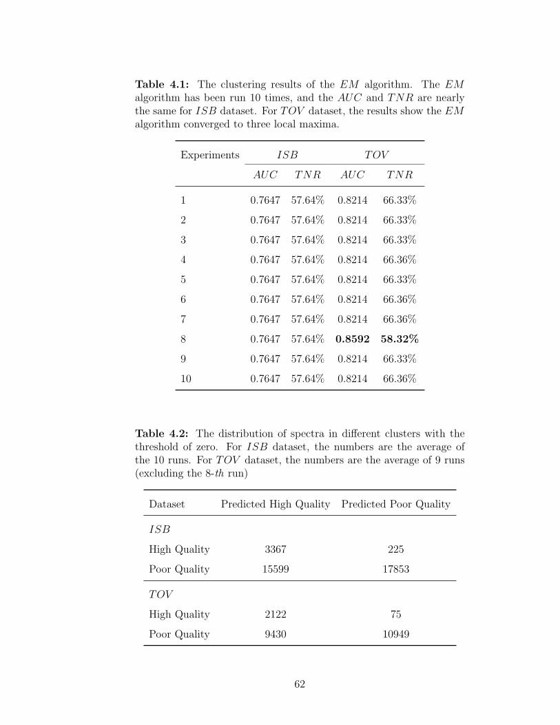
Table 4.1: The clustering results of the EM algorithm. The EMalgorithm has been run 10 times, and the AUC and TNR are nearlythe same for ISB dataset. For TOV dataset, the results show the EMalgorithm converged to three local maxima.

Experiments ISB TOV

AUC TNR AUC TNR

1 0.7647 57.64% 0.8214 66.33%

2 0.7647 57.64% 0.8214 66.33%

3 0.7647 57.64% 0.8214 66.33%

4 0.7647 57.64% 0.8214 66.36%

5 0.7647 57.64% 0.8214 66.33%

6 0.7647 57.64% 0.8214 66.36%

7 0.7647 57.64% 0.8214 66.36%

8 0.7647 57.64% 0.8592 58.32%

9 0.7647 57.64% 0.8214 66.33%

10 0.7647 57.64% 0.8214 66.36%

Table 4.2: The distribution of spectra in different clusters with thethreshold of zero. For ISB dataset, the numbers are the average ofthe 10 runs. For TOV dataset, the numbers are the average of 9 runs(excluding the 8-th run)

Dataset Predicted High Quality Predicted Poor Quality

ISB

High Quality 3367 225

Poor Quality 15599 17853

TOV

High Quality 2122 75

Poor Quality 9430 10949

62

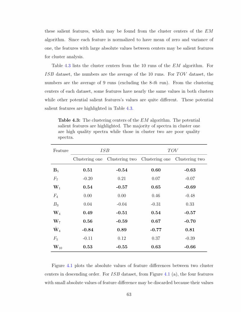
these salient features, which may be found from the cluster centers of the EM

algorithm. Since each feature is normalized to have mean of zero and variance of

one, the features with large absolute values between centers may be salient features

for cluster analysis.

Table 4.3 lists the cluster centers from the 10 runs of the EM algorithm. For

ISB dataset, the numbers are the average of the 10 runs. For TOV dataset, the

numbers are the average of 9 runs (excluding the 8-th run). From the clustering

centers of each dataset, some features have nearly the same values in both clusters

while other potential salient features’s values are quite different. These potential

salient features are highlighted in Table 4.3.

Table 4.3: The clustering centers of the EM algorithm. The potentialsalient features are highlighted. The majority of spectra in cluster oneare high quality spectra while those in cluster two are poor qualityspectra.

Feature ISB TOV

Clustering one Clustering two Clustering one Clustering two

B5 0.51 -0.54 0.60 -0.63

F7 -0.20 0.21 0.07 -0.07

W1 0.54 -0.57 0.65 -0.69

F4 0.00 0.00 0.46 -0.48

B3 0.04 -0.04 -0.31 0.33

W4 0.49 -0.51 0.54 -0.57

W7 0.56 -0.59 0.67 -0.70

W4 -0.84 0.89 -0.77 0.81

F5 -0.11 0.12 0.37 -0.39

W10 0.53 -0.55 0.63 -0.66

Figure 4.1 plots the absolute values of feature differences between two cluster

centers in descending order. For ISB dataset, from Figure 4.1 (a), the four features

with small absolute values of feature difference may be discarded because their values

63

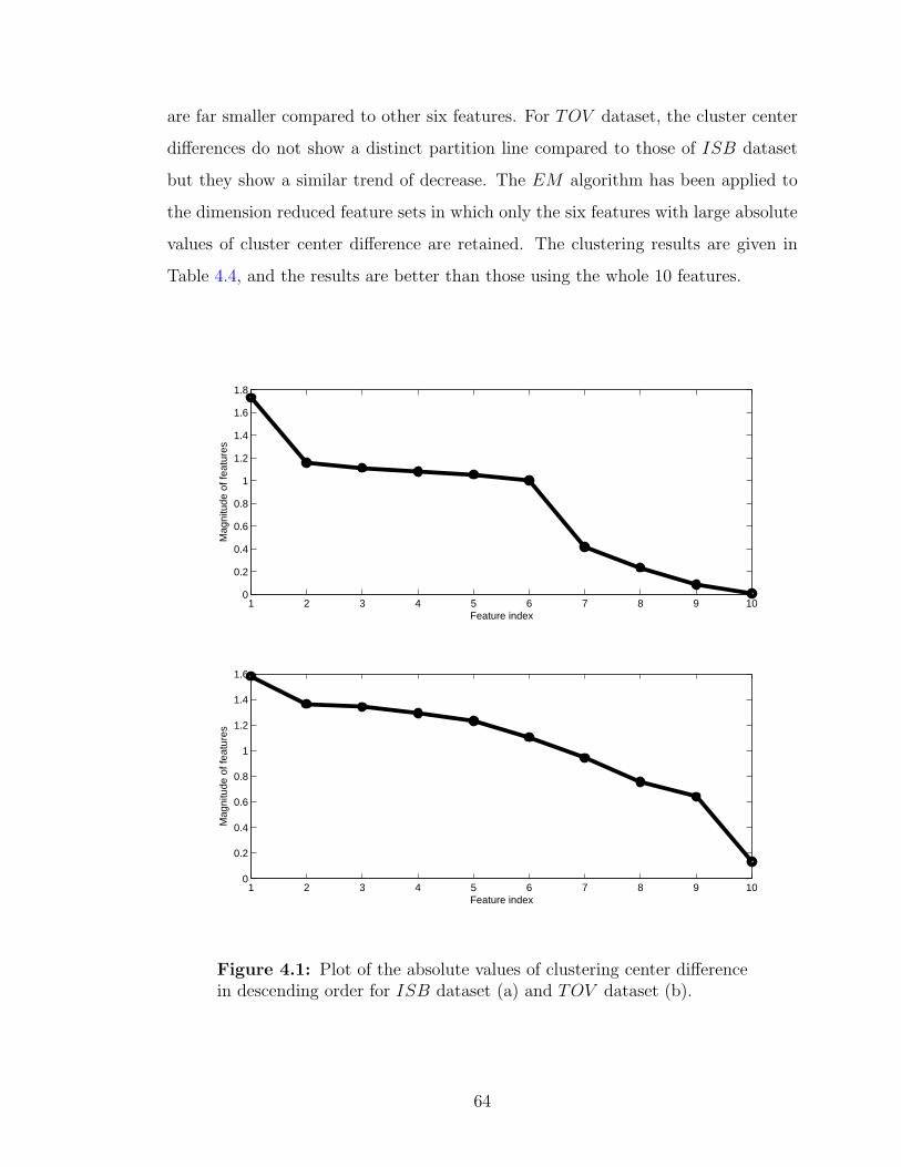
are far smaller compared to other six features. For TOV dataset, the cluster center

differences do not show a distinct partition line compared to those of ISB dataset

but they show a similar trend of decrease. The EM algorithm has been applied to

the dimension reduced feature sets in which only the six features with large absolute

values of cluster center difference are retained. The clustering results are given in

Table 4.4, and the results are better than those using the whole 10 features.

1 2 3 4 5 6 7 8 9 100

0.2

0.4

0.6

0.8

1

1.2

1.4

1.6

1.8

Feature index

Mag

nitu

de o

f fea

ture

s

1 2 3 4 5 6 7 8 9 100

0.2

0.4

0.6

0.8

1

1.2

1.4

1.6

Feature index

Mag

nitu

de o

f fea

ture

s

Figure 4.1: Plot of the absolute values of clustering center differencein descending order for ISB dataset (a) and TOV dataset (b).

64

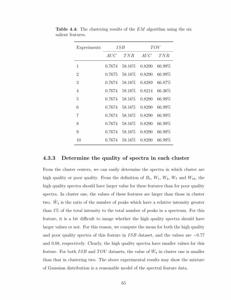
Table 4.4: The clustering results of the EM algorithm using the sixsalient features.

Experiments ISB TOV

AUC TNR AUC TNR

1 0.7674 58.16% 0.8290 66.99%

2 0.7675 58.16% 0.8290 66.99%

3 0.7674 58.16% 0.8289 66.87%

4 0.7674 58.16% 0.8214 66.36%

5 0.7674 58.16% 0.8290 66.99%

6 0.7674 58.16% 0.8290 66.99%

7 0.7674 58.16% 0.8290 66.99%

8 0.7674 58.16% 0.8290 66.99%

9 0.7674 58.16% 0.8290 66.99%

10 0.7674 58.16% 0.8290 66.99%

4.3.3 Determine the quality of spectra in each cluster

From the cluster centers, we can easily determine the spectra in which cluster are

high quality or poor quality. From the definition of B5, W1, W4, W7 and W10, the

high quality spectra should have larger value for these features than for poor quality

spectra. In cluster one, the values of these features are larger than those in cluster

two. W4 is the ratio of the number of peaks which have a relative intensity greater

than 1% of the total intensity to the total number of peaks in a spectrum. For this

feature, it is a bit difficult to image whether the high quality spectra should have

larger values or not. For this reason, we compute the mean for both the high quality

and poor quality spectra of this feature in ISB dataset, and the values are −0.77

and 0.08, respectively. Clearly, the high quality spectra have smaller values for this

feature. For both ISB and TOV datasets, the value of W4 in cluster one is smaller

than that in clustering two. The above experimental results may show the mixture

of Gaussian distribution is a reasonable model of the spectral feature data.

65

Chapter 5

Conclusions and future work

5.1 Conclusions

In this thesis, we have applied several methods for the pre-processing of tandem

mass spectra. Firstly, since about 80% of peaks in a spectrum are noisy peaks, a

novel denoising algorithm is used to filter most noisy peaks. After denoised by the

proposed algorithm, about 69% of peaks in a spectrum can be removed. At the

same time, the number of spectra that can be identified by Mascot search engine

increases by 31.23% and 14.12% for the spectra from two datasets ISB and TOV ,

respectively.

Secondly, in addition to the noise in spectra, most spectra produced by tandem

mass spectrometers are poor quality spectra and they can’t be identified by pep-

tide identification algorithms. Removing these poor quality spectra before peptide

identification can save the time for identifying these uninterpretable spectra, and

decrease false positive rates in peptide identifications. We use machine learning al-

gorithms for the quality assessment of tandem mass spectra. To enable learning,

each spectrum is represented by a fixed length feature vector. The challenging task

for machine learning is to find the discriminative features which can best differentiate

the high quality spectra from the poor quality ones. Therefore, we have designed

several feature selection algorithms to select these discriminative relevant features.

These algorithms include a two-stage recursive feature elimination based on support

vector machine and a sparse logistic regression model. Experimental results show

that supervised machine learning algorithms such as support vector machine can be

trained to remove more than 90% of poor quality spectra without losing more than

66

10% of high quality spectra.

Thirdly, a labeled training set is needed for supervised machine learning algo-

rithms. However, the spectra produced from the same peptide under different ex-

perimental conditions may be quite different, so the supervised machine learning

algorithms’ performance may be degenerated if the training and testing spectra are

from different experiments or different tandem mass spectrometers. We use model-

based clustering algorithms for quality assessment of tandem mass spectra without

the need of a training dataset. Experiments have shown that more than 53% of poor

quality spectra can be safely removed at the expense of removing very minority of

high quality spectra (about 6.26% and 3.41% of high quality spectra of two datasets

ISB and TOV , respectively).

These pre-processing methods improve the reliability of peptide identification

from tandem mass spectra, thus more information can be extracted from tandem

mass spectra. At the same time, as most noisy peaks of spectra and poor quality

spectra are removed, the resources for storing the spectra and the time for identify-

ing the processed spectra are also decreased, even dramatically, e.g., about 70% of

storage space can be saved after the spectra are denoised by the proposed method

in Chapter 2 of this thesis.

5.2 Future work

Based on the workflow proposed in Chapter 1, we have designed several algorithms

to pre-process tandem mass spectra. By the implementation of the algorithms in the

proposed workflow, for an input experimental spectrum, we can output the quality

label of the spectrum as well as the denoised version of this spectrum. However, in

the present workflow, we have not explored the relationship between some modules.

For example, we have not shown the influence of denoising to feature extraction, then

to feature selection and finally to quality assessment. There is a great need to do so

since the denoised spectra have far less peaks than the original undenoised spectra,

and thus denoising spectra can speed up or even help constructing discriminate

67

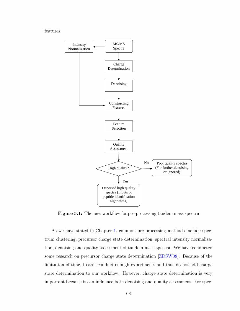
features.

Intensity Normalization

Quality Assessment

Feature Selection

Constructing Features

Denoising

High quality?

Yes

No

Charge Determination

Poor quality spectra (For further denoising

or ignored)

Denoised high quality spectra (Inputs of

peptide identification algorithms)

MS/MS Spectra

Figure 5.1: The new workflow for pre-processing tandem mass spectra

As we have stated in Chapter 1, common pre-processing methods include spec-

trum clustering, precursor charge state determination, spectral intensity normaliza-

tion, denoising and quality assessment of tandem mass spectra. We have conducted

some research on precursor charge state determination [ZDSW08]. Because of the

limitation of time, I can’t conduct enough experiments and thus do not add charge

state determination to our workflow. However, charge state determination is very

important because it can influence both denoising and quality assessment. For spec-

68

trum clustering, it is difficult to be implemented online. Consequently, it is also not

integrated into our workflow.

To improve our present workflow, we proposed the new workflow shown in Figure

5.1. In this workflow, the charge state determination and the filtering model is critical

since the subsequent modules are based on the outputs of these modules.

Note that some modules in the workflow can also be used as post-processing

methods for peptide identifications. For example, the uninterpretable spectra from

peptide identification algorithms can be denoised and then be used for further identi-

fication. For quality assessment algorithms, they can be used to find false negatives,

false positives or post-translational peptides.

69

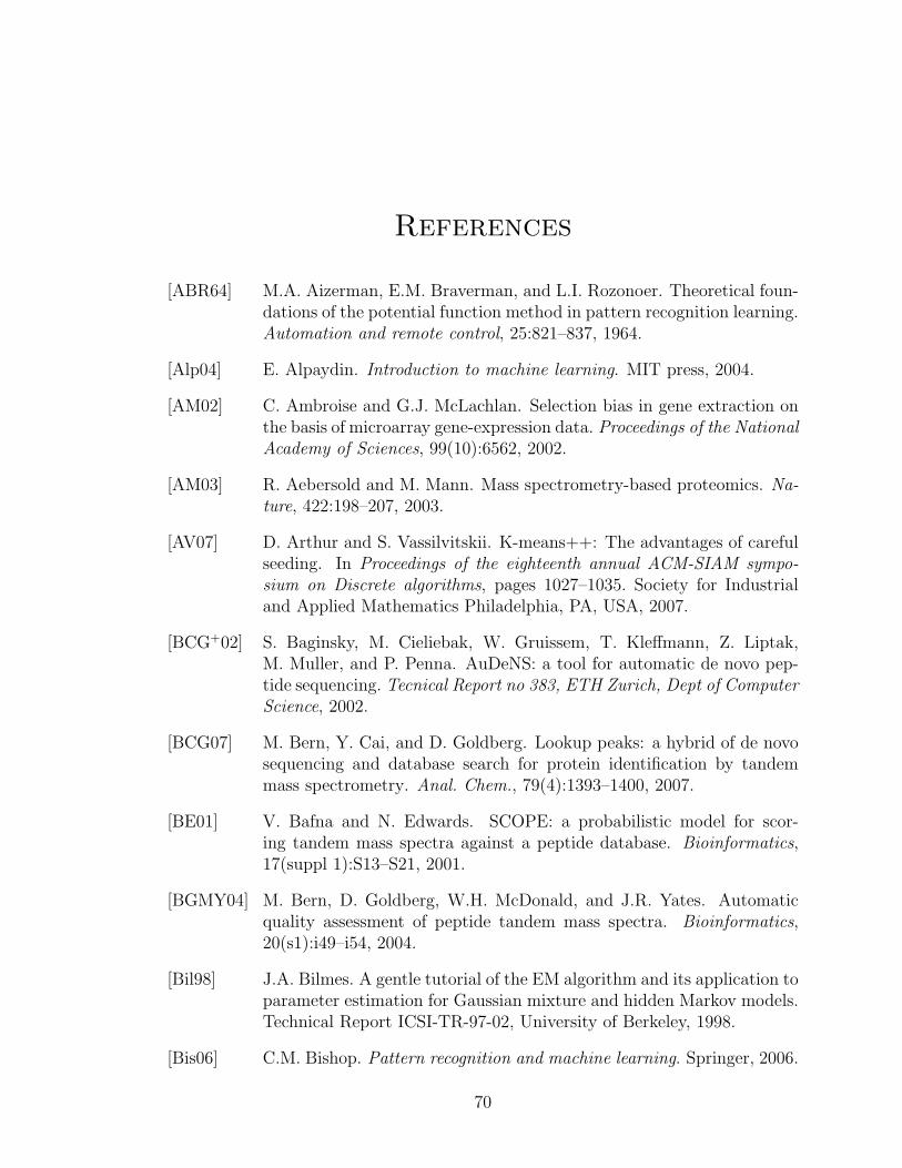
References

[ABR64] M.A. Aizerman, E.M. Braverman, and L.I. Rozonoer. Theoretical foun-dations of the potential function method in pattern recognition learning.Automation and remote control, 25:821–837, 1964.

[Alp04] E. Alpaydin. Introduction to machine learning. MIT press, 2004.

[AM02] C. Ambroise and G.J. McLachlan. Selection bias in gene extraction onthe basis of microarray gene-expression data. Proceedings of the NationalAcademy of Sciences, 99(10):6562, 2002.

[AM03] R. Aebersold and M. Mann. Mass spectrometry-based proteomics. Na-ture, 422:198–207, 2003.

[AV07] D. Arthur and S. Vassilvitskii. K-means++: The advantages of carefulseeding. In Proceedings of the eighteenth annual ACM-SIAM sympo-sium on Discrete algorithms, pages 1027–1035. Society for Industrialand Applied Mathematics Philadelphia, PA, USA, 2007.

[BCG+02] S. Baginsky, M. Cieliebak, W. Gruissem, T. Kleffmann, Z. Liptak,M. Muller, and P. Penna. AuDeNS: a tool for automatic de novo pep-tide sequencing. Tecnical Report no 383, ETH Zurich, Dept of ComputerScience, 2002.

[BCG07] M. Bern, Y. Cai, and D. Goldberg. Lookup peaks: a hybrid of de novosequencing and database search for protein identification by tandemmass spectrometry. Anal. Chem., 79(4):1393–1400, 2007.

[BE01] V. Bafna and N. Edwards. SCOPE: a probabilistic model for scor-ing tandem mass spectra against a peptide database. Bioinformatics,17(suppl 1):S13–S21, 2001.

[BGMY04] M. Bern, D. Goldberg, W.H. McDonald, and J.R. Yates. Automaticquality assessment of peptide tandem mass spectra. Bioinformatics,20(s1):i49–i54, 2004.

[Bil98] J.A. Bilmes. A gentle tutorial of the EM algorithm and its application toparameter estimation for Gaussian mixture and hidden Markov models.Technical Report ICSI-TR-97-02, University of Berkeley, 1998.

[Bis06] C.M. Bishop. Pattern recognition and machine learning. Springer, 2006.

70

[BLY+07] B.M. Balgley, T. Laudeman, L. Yang, T. Song, and C.S. Lee. Com-parative Evaluation of Tandem MS Search Algorithms Using a Target-Decoy Search Strategy. Molecular & Cellular Proteomics, 6(9):1599–1608, 2007.

[Bre98] L. Breiman. Classification and regression trees. Chapman & Hall/CRC,1998.

[BTBP04] N. Bandeira, H. Tang, V. Bafna, and P. Pevzner. Shotgun protein se-quencing by tandem mass spectra assembly. Anal. Chem., 76(24):7221–7233, 2004.

[CB04] R. Craig and R.C. Beavis. TANDEM: matching proteins with tandemmass spectra. Bioinformatics, 20(9):921–922, 2004.

[Cha] D.H. Chace. A layperson’s guide to tandem mass spectrometry andnewborn screening. http://www.savebabies.org/NBS/msms-chace.php.

[CL01] C.C. Chang and C.J. Lin. LIBSVM: a library forsupport vector machines, 2001. Software available athttp://www.csie.ntu.edu.tw/ cjlin/libsvm.

[CM02] D. Comaniciu and P. Meer. Mean shift: a robust approach towardfeature space analysis. IEEE Transactions on Pattern Analysis andMachine Intelligence, 24(5):603–619, 2002.

[CMD+03] J. Colinge, J. Magnin, T. Dessingy, M. Giron, and A. Masselot. Im-proved peptide charge state assignment. Proteomics, 3(8):1434–1440,2003.

[CMG+03] J. Colinge, A. Masselot, M. Giron, T. Dessingy, and J. Magnin. OLAV:Towards high-throughput tandem mass spectrometry data identifica-tion. Proteomics, 3(8):1454–1463, 2003.

[CST00] N. Cristianini and J. Shawe-Taylor. An introduction to support VectorMachines: and other kernel-based learning methods. Cambridge Univ.Pr., 2000.

[CT06] G.C. Cawley and N.L.C. Talbot. Gene selection in cancer classificationusing sparse logistic regression with Bayesian regularization. Bioinfor-matics, 22(19):2348–2355, 2006.

[CT07] K.W. Choo and W.M. Tham. Tandem mass spectrometry data qualityassessment by self-convolution. BMC bioinformatics, 8(1):352, 2007.

[DAC+99] V. Dancik, T.A. Addona, K.R. Clauser, J.E. Vath, and P.A. Pevzner.De novo peptide sequencing via tandem mass spectrometry. Journal ofComputational Biology, 6(3-4):327–342, 1999.

71

[DB04] J.G. Dy and C.E. Brodley. Feature selection for unsupervised learning.The Journal of Machine Learning Research, 5:845–889, 2004.

[DCSL02] M. Dash, K. Choi, P. Scheuermann, and H. Liu. Feature selection forclustering-a filter solution. In Proceedings of the 2002 IEEE Interna-tional Conference on Data Mining (ICDM’02), pages 115–122. IEEEComputer Society Washington, DC, USA, 2002.

[DHS00] R.O. Duda, P.E. Hart, and D.G. Stork. Pattern classification. Wiley-Interscience, 2000.

[DLR77] A.P. Dempster, N.M. Laird, and D.B. Rubin. Maximum likelihood fromincomplete data via the EM algorithm. Journal of the Royal StatisticalSociety. Series B (Methodological), 39(1):1–38, 1977.

[DR05] K. Duan and J.C. Rajapakse. SVM-RFE peak selection for cancer clas-sification with mass spectrometry data. Proc. 3rd Asia-Pacific Bioinf.Conf., 1:191–200, 2005.

[DSPW09] J. Ding, J. Shi, G.G. Poirier, and F.X. Wu. A novel approach to de-noising tandem mass spectra. Proteome Science, 7(9), 2009.

[DSW09] J. Ding, J. Shi, and F.X. Wu. Quality assessment of tandem mass spec-tra by using a weighted k-means. Clinical Proteomics, 2009. Accepted.

[DSZW08] J. Ding, J. Shi, A.M. Zou, and F.X. Wu. Feature selection for tandemmass spectrum quality assessment. In IEEE International Conferenceon Bioinformatics and Biomedicine (IEEE BIBM 2008), pages 310–313,2008.

[DW09a] J. Ding and F.X. Wu. Feature selection for tandem mass spectrumquality assessment via sparse logistic regression. In The 3rd Inter-national Conference on Bioinformatics and Biomedical Engineering(iCBBE 2009), 2009. Accepted.

[DW09b] J. Ding and F.X. Wu. Model based clustering for quality assessment oftandem mass spectra. 2009. In preparation.

[Efr79] B. Efron. Bootstrap methods: another look at the jackknife. The Annalsof Statistics, 7(1):1–26, 1979.

[EHFG05] J.E. Elias, W. Haas, B.K. Faherty, and S.P. Gygi. Comparative eval-uation of mass spectrometry platforms used in large-scale proteomicsinvestigations. Nat. Methods, 2(9):667–675, 2005.

[EMY94] J.K. Eng, A.L. McCormack, and J.R. Yates. An approach to correlatetandem mass spectral data of peptides with amino acid sequences in aprotein database. J. Am. Soc. Mass Spectrom., 5(11):976–989, 1994.

72

[FA05] J. Falkner and P. Andrews. Fast tandem mass spectra-based proteinidentification regardless of the number of spectra or potential modifica-tions examined. Bioinformatics, 21(10):2177–2184, 2005.

[Faw04] T. Fawcett. ROC graphs: notes and practical considerations for re-searchers. Machine Learning, 31, 2004.

[FBS+08] A.M. Frank, N. Bandeira, Z. Shen, S. Tanner, S.P. Briggs, R.D. Smith,and P.A. Pevzner. Clustering millions of tandem mass spectra. J. Pro-teome Res., 7(1):113–122, 2008.

[FD07] B.J. Frey and D. Dueck. Clustering by passing messages between datapoints. Science, 315(5814):972–976, 2007.

[FMH+07] K. Flikka, J. Meukens, K. Helsens, J. Vandekerckhove, I. Eidhammer,K. Gevaert, and L. Martens. Implementation and application of a ver-satile clustering tool for tandem mass spectrometry data. Proteomics,7(18):3245–3258, 2007.

[FMV+06] K. Flikka, L. Martens, J. Vandekerckhove, K. Gevaert, and I. Eidham-mer. Improving the reliability and throughput of mass spectrometry-based proteomics by spectrum quality filtering. Proteomics, 6(7):2086–2094, 2006.

[FNC07] J. Feng, D.Q. Naiman, and B. Cooper. Probability model for assessingproteins assembled from peptide sequences inferred from tandem massspectrometry data. Anal. Chem, 79(10):3901–3911, 2007.

[FP05] A. Frank and P. Pevzner. PepNovo: de novo peptide sequencing viaprobabilistic network modeling. Anal. Chem., 77(4):964–973, 2005.

[FRR+05] B. Fischer, V. Roth, F. Roos, J. Grossmann, S. Baginsky, P. Widmayer,W. Gruissem, and J.M. Buhmann. NovoHMM: a hidden Markov modelfor de novo peptide sequencing. Anal. Chem., 77(22):7265–7273, 2005.

[Fuk90] K. Fukunaga. Introduction to Statistical Pattern Recognition. AcademicPress, 1990.

[GGNZ06] I. Guyon, S. Gunn, M. Nikravesh, and L.A. Zadeh. Feature extraction:foundations and applications (studies in fuzziness and soft computing).Springer, 2006.

[GKPW03] M. Gentzel, T. Kocher, S. Ponnusamy, and M. Wilm. Preprocessing oftandem mass spectrometric data to support automatic protein identifi-cation. Proteomics, 3(8):1597–1610, 2003.

[GMK+04] L.Y. Geer, S.P. Markey, J.A. Kowalak, L. Wagner, M. Xu, D.M. May-nard, X. Yang, W. Shi, and S.H. Bryant. Open mass spectrometrysearch algorithm. Journal of Proteome Research, 3(5):958–964, 2004.

73

[GRC+05] J. Grossmann, F.F. Roos, M. Cieliebak, Z. Liptak, L.K. Mathis,M. Muller, W. Gruissem, and S. Baginsky. AUDENS: a tool for au-tomated peptide de novo sequencing. J. Proteome Res., 4(1):768–771,2005.

[GS00] I. Guyon and D.G. Stork. Advances in large margin classifiers, chapterLinear discriminant and support vector classifiers, pages 147–169. MITPress, 2000.

[GSM03] B. Georgescu, I. Shimshoni, and P. Meer. Mean shift based clusteringin high dimensions: a texture classification example. Proceedings of theNinth IEEE International Conference on Computer Vision (ICCV’03),pages 456–463, 2003.

[Gue08] S. Guerif. Unsupervised Variable Selection: when random rankingssound as irrelevancy. JMLR: Workshop and Conference Proceedings,4:163–177, 2008.

[GW07] R.C. Gonzalez and R.E. Woods. Digital image processing. Prentice Hall,2007.

[GWBV02] I. Guyon, J. Weston, S. Barnhill, and V. Vapnik. Gene selection forcancer classification using support vector machines. Machine Learning,46(1):389–422, 2002.

[HCM+08] T. Hesterberg, N. Choi, L. Meier, ETH Zuerich, C. Fraley, et al. Leastangle and L 1 penalized regression: A review. volume 2, pages 61–93.American Statistical Association, 2008.

[HCN05] X. He, D. Cai, and P. Niyogi. Laplacian score for feature selection.Advances in Neural Information Processing Systems, 18, 2005.

[HK08] M. Hilario and A. Kalousis. Approaches to dimensionality reduction inproteomic biomarker studies. Briefings in Bioinformatics, 9(2):108–118,2008.

[HKPM06] M. Hilario, A. Kalousis, C. Pellegrini, and M. Muller. Processing andclassification of protein mass spectra. Mass Spectrometry Reviews, 25(3),2006.

[HMA06] P. Hernandez, M. Muller, and R.D. Appel. Automated protein iden-tification by tandem mass spectrometry: Issues and strategies. MassSpectrometry Reviews, 25(2):235–254, 2006.

[HMM+05] T. Hesterberg, S. Monaghan, D.S. Moore, A. Clipson, and R. Epstein.The practice of business statistics, (fifth edition), chapter Bootstrapmethods and permutation tests. 2005.

74

[HS01] S. Hua and Z. Sun. Support vector machine approach for protein sub-cellular localization prediction. Bioinformatics, 17(8):721–728, 2001.

[HTF01] T. Hastie, R. Tibshirani, and J. Friedman. The elements of statisticallearning: data mining, inference, and prediction. Springer, 2001.

[Hun93] L. Hunter. Artificial Intelligence and Molecular Biology, chapter Molec-ular biology for computer scientists, pages 1–46. MIT Press, 1993.

[HZM00] D.M. Horn, R.A. Zubarev, and F.W. McLafferty. Automated de novosequencing of proteins by tandem high-resolution mass spectrometry,2000.

[JMF99] AK Jain, MN Murty, and PJ Flynn. Data clustering: a review. ACMcomputing surveys, 31(3):264–323, 1999.

[JP04] N.C. Jones and P. Pevzner. An introduction to bioinformatics algo-rithms. MIT Press Cambridge, Mass, 2004.

[KHG08] J. Khatun, E. Hamlett, and M.C. Giddings. Incorporating sequenceinformation into the scoring function: a hidden Markov model for im-proved peptide identification. Bioinformatics, 24(5):674–681, 2008.

[KKB07] K. Koh, S.J. Kim, and S. Boyd. An interior-point method for large-scale L1-regularized logistic regression. Journal of Machine LearningResearch, 8:1519–1555, 2007.

[KL07] N. Kang and H.W. Leong. Algorithm for peptide sequencing by tandemmass spectrometry based on better preprocess and anti-symmetric com-putational model. Proceedings of the 2007 IEEE Computational SystemsBioinformatics Conference (CSB’07), 2007.

[KNKA02] A. Keller, A.I. Nesvizhskii, E. Kolker, and R. Aebersold. Empirical sta-tistical model to estimate the accuracy of peptide identifications madeby MS/MS and database search. Anal. Chem., 74(20):5383–5392, 2002.

[KPN+02] A. Keller, S. Purvine, AI Nesvizhskii, S. Stolyar, DR Goodlett, andE. Kolker. Experimental protein mixture for validating tandem massspectral analysis. OMICS, 6(2):207–212, 2002.

[KS00] M. Kinter and N.E. Sherman. Protein sequencing and identificationusing tandem mass spectrometry. Wiley, 2000.

[KSC+05] E.A. Kapp, F. Schutz, L.M. Connolly, J.A. Chakel, J.E. Meza, C.A.Miller, D. Fenyo, J.K. Eng, J.N. Adkins, G.S. Omenn, et al. An evalua-tion, comparison, and accurate benchmarking of several publicly avail-able MS/MS search algorithms: sensitivity and specificity analysis. Pro-teomics, 5(13):3475–3490, 2005.

75

[KWMN05] AA Klammer, CC Wu, MJ MacCoss, and WS Noble. Peptide chargestate determination for low-resolution tandem mass spectra. In Pro-ceedings of the IEEE Computational Systems Bioinformatics Conference(CSB 2005), pages 175–185, 2005.

[LBB+07] J. Liu, A.W. Bell, J.J.M. Bergeron, C.M. Yanofsky, B. Carrillo, C.E.H.Beaudrie, and R.E. Kearney. Methods for peptide identification byspectral comparison. Proteome Science, 5(3), 2007.

[LFJ04] MHC Law, MAT Figueiredo, and AK Jain. Simultaneous feature se-lection and clustering using mixture models. IEEE Transactions onPattern Analysis and Machine Intelligence, 26(9):1154–1166, 2004.

[LM98] H. Liu and H. Motoda. Feature selection for knowledge discovery anddata mining. Springer, 1998.

[LM07] H. Liu and H. Motoda. Computational methods of feature selection.Chapman & Hall/CRC, 2007.

[LTK+04] R.D. LeDuc, G.K. Taylor, Y.B. Kim, T.E. Januszyk, L.H. Bynum, J.V.Sola, J.S. Garavelli, and N.L. Kelleher. ProSight PTM: an integratedenvironment for protein identification and characterization by top-downmass spectrometry. Nucleic Acids Research, 32(suppl 2):W340–W345,2004.

[LZN08] L. Li, J. Zhang, and R.M. Neal. A method for avoiding bias fromfeature selection with application to Naive Bayes classification models.Bayesian Analysis, 3(1):171–196, 2008.

[Mac67] J.B. MacQueen. Some methods for classification and analysis of mul-tivariate observations. In Proceedings of the fifth Berkeley symposiumon mathematical statistics and probability, pages 281–297. University ofCalifornia Press, 1967.

[Mac03] D.J.C. MacKay. Information theory, inference, and learning algorithms.Cambridge University Press New York, 2003.

[Mal99] S. Mallat. A wavelet tour of signal processing. Academic press, 1999.

[MH08] S. Ma and J. Huang. Penalized feature selection and classification inbioinformatics. Briefings in Bioinformatics, 9(5):392–403, 2008.

[MMP02] P. Mitra, CA Murthy, and SK Pal. Unsupervised feature selection usingfeature similarity. IEEE Transactions on Pattern Analysis and MachineIntelligence, 24(3):301–312, 2002.

[MRH+06] N. Mujezinovic, G. Raidl, JR Hutchins, J.M. Peters, K. Mechtler, andF. Eisenhaber. Cleaning of raw peptide MS/MS spectra: improved pro-tein identification following deconvolution of multiply charged peaks,

76

isotope clusters, and removal of background noise. Proteomics,6(19):5117–5131, 2006.

[MS90] P. Maragos and RW Schafer. Morphological systems for multidimen-sional signal processing. Proceedings of the IEEE, 78(4):690–710, 1990.

[Mur10] K. Murphy. Machine learning: a probabilistic approach. MIT Press,2010. In preparation.

[MZH+03] B. Ma, K. Zhang, C. Hendrie, C. Liang, M. Li, A. Doherty-Kirby, andG. Lajoie. PEAKS: powerful software for peptide de novo sequencing bytandem mass spectrometry. Rapid communications in mass spectrome-try, 17(20):2337–2342, 2003.

[MZL05] B. Ma, K. Zhang, and C. Liang. An effective algorithm for peptidede novo sequencing from MS/MS spectra. Journal of Computer andSystem Sciences, 70(3):418–430, 2005.

[Nob06] W.S. Noble. What is a support vector machine? Nature Biotechnology,24(12):1565–1567, 2006.

[NP06] S. Na and E. Paek. Quality assessment of tandem mass spectra based oncumulative intensity normalization. J. Proteome Res., 5(12):3241–3248,2006.

[NPL08] S. Na, E. Paek, and C. Lee. CIFTER: automated charge-state determi-nation for peptide tandem mass spectra. Anal. Chem., 80(5):1520–1528,2008.

[NRG+06] A.I. Nesvizhskii, F.F. Roos, J. Grossmann, M. Vogelzang, J.S. Eddes,W. Gruissem, S. Baginsky, and R. Aebersold. Dynamic spectrum qualityassessment and iterative computational analysis of shotgun proteomicdata toward more efficient identification of post-translational modifica-tions, sequence polymorphisms, and novel peptides. Molecular & Cel-lular Proteomics, 5(4):652–670, 2006.

[NTV+05] C. Narasimhan, D.L. Tabb, N.C. VerBerkmoes, M.R. Thompson, R.L.Hettich, and E.C. Uberbacher. MASPIC: intensity-based tandem massspectrometry scoring scheme that improves peptide identification athigh confidence. Anal. Chem, 77(23):7581–7593, 2005.

[NVA07] A.I. Nesvizhskii, O. Vitek, and R. Aebersold. Analysis and validationof proteomic data generated by tandem mass spectrometry. Naturemethods, 4(10):787–797, 2007.

[PKK04] S. Purvine, N. Kolker, and E. Kolker. Spectral quality assessment forhigh-throughput tandem mass spectrometry proteomics. Omics A Jour-nal of Integrative Biology, 8(3):255–265, 2004.

77

[PPDC99] D.N. Perkins, D.J.C Pappin, Creasy D.M., and J.S. Cottrell.Probability-based protein identification by searching sequence databasesusing mass spectrometry data. Electrophoresis, 20(18):3551–3567, 1999.

[RCA+04] T. Rejtar, H.S. Chen, V. Andreev, E. Moskovets, and B.L. Karger.Increased identification of peptides by enhanced data processing of high-resolution MALDI TOF/TOF mass spectra prior to database searching.Anal. Chem., 76(20):6017–6028, 2004.

[RD06] A.E. Raftery and N. Dean. Variable selection for model-based cluster-ing. Journal of the American Statistical Association, 101(473):168–178,2006.

[RGE03] A. Rakotomamonjy, I. Guyon, and A. Elisseeff. Variable selection usingSVM-based criteria. Journal of Machine Learning Research, 3:1357–1370, 2003.

[SAdP08] Y. Saeys, T. Abeel, and YV de Peer. Towards robust feature selectiontechniques. In Proceedings of Benelearn, pages 45–46, 2008.

[SED+02] R.G. Sadygov, J. Eng, E. Durr, A. Saraf, H. McDonald, M.J. MacCoss,and J.R. Yates III. Code developments to improve the efficiency of au-tomated MS/MS spectra interpretation. Journal of Proteome Research,1(3):211–215, 2002.

[SHH08] R.G. Sadygov, Z. Hao, and A.F.R. Huhmer. Charger: combinationof signal processing and statistical learning algorithms for precursorcharge-state determination from electron-transfer dissociation spectra.Anal. Chem, 80(2):376–386, 2008.

[SIL07] Y. Saeys, I. Inza, and P. Larranaga. A review of feature selection tech-niques in bioinformatics. Bioinformatics, 23(19):2507–2517, 2007.

[SM00] J. Shi and J. Malik. Normalized cuts and image segmentation. IEEETransactions on Pattern Analysis and Machine Intelligence, 22(8):888–905, 2000.

[SMF+06] J. Salmi, R. Moulder, J.J. Filen, O.S. Nevalainen, T.A. Nyman, R. La-hesmaa, and T. Aittokallio. Quality classification of tandem mass spec-trometry data. Bioinformatics, 22(4):400–406, 2006.

[SS02] B. Scholkopf and A.J. Smola. Learning with kernels. MIT press Cam-bridge, Mass, 2002.

[SYI03] R.G. Sadygov and J.R. Yates III. A hypergeometric probability modelfor protein identification and validation using tandem mass spectral dataand protein sequence databases. Anal. Chem, 75(15):3792–3798, 2003.

78

[TEYI01] D.L. Tabb, J.K. Eng, and J.R. Yates III. Protein Identification bySEQUEST. Proteome Research: Mass Spectrometry (James, P. ed.),pages 125–142, 2001.

[Tib96] R. Tibshirani. Regression shrinkage and selection via the lasso. Journalof the Royal Statistical Society, 58(issue 1):267–288, 1996.

[TMW+03] D.L. Tabb, M.J. MacCoss, C.C. Wu, S.D. Anderson, and J.R. Yates.Similarity among tandem mass spectra from proteomic experiments: de-tection, significance, and utility. Anal. Chem., 75(10):2470–2477, 2003.

[TSF+05] S. Tanner, H. Shu, A. Frank, L. Wang, E. Zandi, M. Mumby, P.A.Pevzner, and V. Bafna. Inspect: fast and accurate identification ofpost-translationally modified peptides from tandem mass spectra. Anal.Chem., 77(14):4626–4639, 2005.

[TSS+06] D.L. Tabb, M.B. Shah, M.B. Strader, H.M. Connelly, R.L. Hettich, andG.B. Hurst. Determination of peptide and protein ion charge states byFourier transformation of isotope-resolved mass spectra. Journal of theAmerican Society for Mass Spectrometry, 17(7):903–915, 2006.

[TZH07] Y. Tang, Y.Q. Zhang, and Z. Huang. Development of two-stage SVM-RFE gene selection strategy for microarray expression data analysis.IEEE/ACM Transactions on Computational Biology and Bioinformat-ics, 4(3):365–381, 2007.

[Vap98] V.N. Vapnik. Statistical learning theory. Wiley New York, 1998.

[Vap00] V.N. Vapnik. The nature of statistical learning theory. Springer, 2000.

[VGLH06] R. Varshavsky, A. Gottlieb, M. Linial, and D. Horn. Novel unsupervisedfeature filtering of biological data. Bioinformatics, 22(14), 2006.

[Vin93] L. Vincent. Morphological grayscale reconstruction in image analysis:applications and efficient algorithms. IEEE Transactions on Image Pro-cessing, 2(2):176–201, 1993.

[WDP08] F.X. Wu, J. Ding, and G.G. Poirier. An approach to assess peptide massspectral quality without prior information. International Journal ofFunctional Informatics and Personalised Medicine, 5(2):140–155, 2008.

[Web02] A. Webb. Statistical pattern recognition. Wiley-Interscience, 2002.

[WGDP06] F-X. Wu, P. Gagne, A. Droit, and G-G. Poirier. RT-PSM, a real-timeprogram for peptide-spectrum matching with statistical significance.Rapid communications in mass spectrometry, 20(8):1199–1208, 2006.

[WGDP08] F.X. Wu, P. Gagne, A. Droit, and G.G. Poirier. Quality assessmentof peptide tandem mass spectra. BMC Bioinformatics, 9(suppl:6):S13,2008.

79

[WSCC07] J.W.H. Wong, M.J. Sullivan, H.M. Cartwright, and G. Cagney. msm-sEval: tandem mass spectral quality assignment for high-throughputproteomics. BMC Bioinformatics, 8(1), 2007.

[WTE07] X Wu, C.W. Tsebg, and N. Edwards. HMMatch: peptide identifica-tion by spectral matching of tandem mass spectra using hidden Markovmodels. Journal of Computational biology, 14(8), 2007.

[WYC06] Y. Wan, A. Yang, and T. Chen. PepHMM: a hidden Markov modelbased scoring function for mass spectrometry database search. Anal.Chem., 78(2):432–437, 2006.

[XGB+05] M. Xu, L.Y. Geer, S.H. Bryant, J.S. Roth, J.A. Kowalak, D.M. May-nard, and S.P. Markey. Assessing data quality of peptide mass spectraobtained by quadrupole ion trap mass spectrometry. J. Proteome Res.,4(2):300–305, 2005.

[ZAS02] N. Zhang, R. Aebersold, and B. Schwikowski. ProbID: a probabilis-tic algorithm to identify peptides through sequence database searchingusing tandem mass spectral data. Proteomics, 2(10):1406–1412, 2002.

[ZDSW08] A.M. Zou, J. Ding, J Shi, and F.X. Wu. Charge state determination ofpeptide tandem mass spectra using support vector machine (SVM). InProceedings of the 8th IEEE International Conference on Bioinformaticsand Bioengineering (BIBE 2008), 2008.

[ZHL+08] J. Zhang, S. He, CX Ling, X. Cao, R. Zeng, and W. Gao. PeakS-elect: preprocessing tandem mass spectra for better peptide identifi-cation. Rapid communications in mass spectrometry, 22(8):1203–1212,2008.

[ZL07] Z. Zhao and H. Liu. Semi-supervised feature selection via spectral anal-ysis. In Proceedings of the 2007 SIAM International Conference on DataMining, pages 641–646, 2007.

[ZLS+06] X. Zhang, X. Lu, Q. Shi, XQ Xu, HC Leung, L.N. Harris, J.D. Iglehart,A. Miron, J.S. Liu, and W.H. Wong. Recursive SVM feature selectionand sample classification for mass-spectrometry and microarray data.BMC Bioinformatics, 7(1):S13, 2006.

[ZSZ+06] Z. Zhang, S. Sun, X. Zhu, S. Chang, X. Liu, C. Yu, D. Bu, and R. Chen.A novel scoring schema for peptide identification by searching proteinsequence databases using tandem mass spectrometry data. BMC Bioin-formatics, 7(222), 2006.

[ZWDP09] A.M. Zou, F.X. Wu, J. Ding, and G.G. Poirier. Quality assessmentof tandem mass spectra using support vector machine (SVM). BMCBioinformatics, 10(Suppl 1):S49, 2009.

80