Embed Size (px)
Citation preview
Pre-Aerosol, Clouds, and ocean Ecosystem (PACE) Mission
Science Definition Team Report
October 16, 2012

PACE Mission Science Definition Team Report
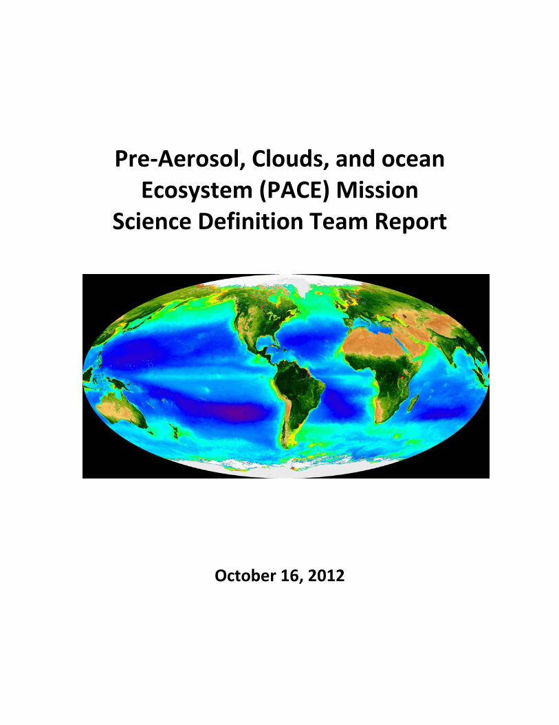
Cover: global image obtained by the Sea-Viewing Wide Field of View Sensor (SeaWiFS). Image available on the NASA Ocean Color Web: (http://oceancolor.gsfc.nasa.gov/).
PACE Mission Science Definition Team Report
PACE Science Definition Team Chair: Del Castillo, Carlos (Johns Hopkins University Applied Physics Laboratory) Deputy Chair: Platnick, Steve (NASA Goddard Space Flight Center)
SDT members: Antoine, David (Laboratoire d’Océanographie de Villefranche, France) Balch, Barney (Bigelow Laboratory for Ocean Sciences) Behrenfeld, Mike (Oregon State University) Boss, Emmanuel (University of Maine) Cairns, Brian (NASA Goddard Institute for Space Studies) Chowdhary, Jacek (NASA Goddard Institute for Space Studies) DaSilva, Arlindo (NASA Goddard Space Flight Center) Diner, David (NASA Jet Propulsion Laboratory) Dubovik, Oleg (University of Lille, France) Franz, Bryan (NASA Goddard Space Flight Center) Frouin, Robert (University California, San Diego - Scripps Institution of Oceanography) Gregg, Watson (NASA Goddard Space Flight Center) Huemmrich, K. Fred (NASA Goddard Space Flight Center [University of Maryland,
Baltimore County]) Kahn, Ralph (NASA Goddard Space Flight Center) Marshak, Alexander (NASA Goddard Space Flight Center) Massie, Steve (National Center for Atmospheric Research) McClain, Charles (NASA Goddard Space Flight Center) McNaughton, Cameron (Golder Associates Ltd. [Canada], University of Hawai`i
at Mānoa) Meister, Gerhard (NASA Goddard Space Flight Center) Mitchell, Greg (University California, San Diego - Scripps Institution of Oceanography) Muller-Karger, Frank (University of South Florida) Puschell, Jeffery (Raytheon) Riedi, Jerome (University of Lille, France) Siegel, David (University California, Santa Barbara) Wang, Menghua (National Oceanic and Atmospheric Administration/National
Environmental Satellite, Data, and Information Service/Center for Satellite Applications and Research)
Werdell, Jeremy (NASA Goddard Space Flight Center)
i
PACE Mission Science Definition Team Report
Acknowledgements The PACE Science Definition Team acknowledges the following scientists who contributed with analysis, figures, and text to this report.
• Zia Ahmad (Science & Data Systems, Inc., NASA Goddard Space Flight Center)
• Odele Coddington (University of Colorado/Laboratory for Atmospheric and Space Physics)
• Kirk D. Knobelspiesse (Oak Ridge Associated Universities)
• Robert Levy (Science Systems and Applications, Inc.,NASA Goddard Space Flight Center)
• John Martonchik (NASA Jet Propulsion Laboratory)
• Kerry Meyer (Goddard Earth Sciences Technology and Research/Universities Space Research Association /NASA Goddard Space Flight Center)
• Ali H.Omar (NASA/Langley Research Center)
• Fred Patt (Science Applications International Corporation, NASA Goddard Space Flight Center)
• Lorraine Remer (University of Maryland, Baltimore County/Joint Center for Earth Systems Technology)
• Andy Sayer (NASA Goddard Space Flight Center)
• Sebastian Schmidt (University of Colorado/Laboratory for Atmospheric and Space Physics)
• Maria A. Tzortziou (University of Maryland/Earth System Science Interdisciplinary Center)
The Science Definition Team also wishes to acknowledge the Engineering Team from NASA Goddard Space Flight Center, whose experience and expertise were invaluable to this effort: Angela Mason, James (Jay) Smith, Richard (Rick) Wesenberg, and Chi Wu.
The Science Definition Team is especially thankful for the work of our technical editor Lena Braatz (Booz Allen Hamilton). Ms. Braatz’s heroic efforts made this a readable and well organized report.
The team also wants to recognize Ed Carter, Dennis McGillicuddy, Larry Di Girolamo, Ed Knight, David Humm, Galen McKinley, Tom Stone, Brian Lottman, and Vyacheslav Suslin for reviewing the report and providing useful commentary and corrections.
We thank Paula Bontempi, Betsy Edwards, Hal Maring, and Woody Turner from NASA-HQ for making the PACE mission possible and for providing the organizational backbone and programmatic guidance to the Science Definition Team.
ii

PACE Mission Science Definition Team Report
This report is a comprehensive and detailed treatise on the science, measurements, and mission requirements necessary for a successful PACE mission. It represents many hours of arduous work by a group of very dedicated and talented scientists. To them goes all the credit. Any errors, omissions, and deficiencies found in this report are my responsibility.
Carlos E. Del Castillo, The Johns Hopkins University/APL Chair, PACE Science Definition Team
iii
PACE Mission Science Definition Team Report
Table of Contents PACE Science Definition Team ............................................................................................. i
Acknowledgements ..............................................................................................................ii
Executive Summary ............................................................................................................. ix
1 Introduction ................................................................................................................ 1
1.1 The Science of PACE ............................................................................................. 1
1.2 The PACE Science Definition Team Philosophy and Methods ............................. 1
1.3 Structure of the Report ........................................................................................ 2
2 Scientific Objectives .................................................................................................... 4
2.1 Introduction .......................................................................................................... 4
2.2 Ocean Ecosystems and Biogeochemistry ............................................................. 4
2.2.1 Threshold Ocean Science Questions ............................................................. 6
2.2.2 Advancing Ocean Science with PACE .......................................................... 10
2.3 Atmosphere: Aerosols and Clouds ..................................................................... 41
2.3.1 Aerosols ....................................................................................................... 47
2.3.2 Clouds .......................................................................................................... 59
2.4 Terrestrial Ecology .............................................................................................. 74
2.4.1 Top-order Goal Terrestrial Ecology Science Questions .............................. 75
2.4.2 Advancing Terrestrial Science with PACE ................................................... 78
2.4.3 Issues and Solutions .................................................................................... 78
2.5 Watersheds and Lakes ....................................................................................... 79
2.5.1 Importance of Lakes and Watersheds to the Carbon Cycle and the Exchange of Biogeochemical Elements between Land and Sea ............................... 79
2.5.2 Spatial and Temporal Scales Required to Characterize Lakes and Watersheds ............................................................................................................... 80
2.5.3 Characterizing Water Types in Inland Waters ............................................ 81
iv
PACE Mission Science Definition Team Report
2.5.4 Atmospheric Correction Requirements ...................................................... 82
2.5.5 Relevance to NASA Goals in Climate Science ............................................. 83
3 PACE Science-Driven Measurement Requirements ................................................. 84
3.1 Introduction ........................................................................................................ 84
3.2 Ocean Ecology and Biogeochemistry ................................................................. 84
3.2.1 Orbit ............................................................................................................ 85
3.2.2 Spatial and Temporal Coverage .................................................................. 85
3.2.3 Navigation and Registration ....................................................................... 87
3.2.4 Instrument Performance Tracking .............................................................. 87
3.2.5 Instrument Artifacts .................................................................................... 89
3.2.6 Spatial Resolution ....................................................................................... 94
3.2.7 Atmospheric Corrections ............................................................................ 95
3.2.8 Science Spectral Bands ............................................................................... 98
3.2.9 Signal-to-noise .......................................................................................... 100
3.2.10 Data Processing, Reprocessing, and Distribution ..................................... 103
3.2.11 Summary of PACE Ocean Science Measurement Requirements ............. 106
3.2.12 Ocean Science Measurement Goals ......................................................... 108
3.2.13 Atmospheric Correction Topics Relevant to PACE Ocean Retrievals ....... 110
3.3 PACE Atmosphere Measurement Requirements ............................................. 118
3.3.1 Orbit .......................................................................................................... 120
3.3.2 Spatial and Temporal Coverage ................................................................ 120
3.3.3 Navigation and Registration ..................................................................... 120
3.3.4 Instrument Performance Tracking ............................................................ 120
3.3.5 Instrument Artifacts .................................................................................. 121
3.3.6 Spatial Resolution ..................................................................................... 121
3.3.7 Atmospheric Corrections .......................................................................... 121
v
PACE Mission Science Definition Team Report
3.3.8 Aerosol and Cloud Science Spectral Bands ............................................... 121
3.3.9 Signal-to-noise .......................................................................................... 122
3.3.10 Data Processing, Reprocessing, and Distribution ..................................... 122
3.3.11 Summary of Cloud and Aerosol Augmentations to the Baseline OCI Imager 122
3.4 Terrestrial Ecology ............................................................................................ 124
4 PACE Spacecraft and Mission Support Requirements ............................................ 125
4.1 Introduction ...................................................................................................... 125
4.2 Launch Vehicle ................................................................................................. 125
4.3 Spacecraft Requirements ................................................................................. 125
4.4 Onboard Calibration Requirements ................................................................. 129
4.4.1 Long-term Degradation Monitoring ......................................................... 130
4.4.2 Short-term Degradation Trending ............................................................ 133
4.4.3 Spectral Monitoring .................................................................................. 134
4.4.4 Spatial Monitoring .................................................................................... 134
4.5 Mission Operations .......................................................................................... 135
4.5.1 Orbit Maintenance .................................................................................... 135
4.5.2 Sensor Command Sequences .................................................................... 135
4.5.3 Solar Diffuser Calibration and Spectral Alignment Data Acquisition ........ 135
4.5.4 Lunar Data Acquisition (Monthly) ............................................................. 136
4.5.5 Sensor Tilt Sequences (Each Orbit) ........................................................... 137
4.5.6 Data Downlink Scheduling (Each Orbit) .................................................... 137
4.5.7 Flight Software .......................................................................................... 137
4.5.8 Sensor and Spacecraft Health and Safety Telemetry, Data Analysis, and Data Archival ........................................................................................................... 137
4.5.9 Anomaly Detection, Investigation, Response and Resolution .................. 138
4.5.10 Science Operations Management ............................................................. 138
vi
PACE Mission Science Definition Team Report
4.6 Field Program Requirements ........................................................................... 138
4.6.1 Oceans ....................................................................................................... 139
4.6.2 Aerosols ..................................................................................................... 150
4.6.3 Clouds ........................................................................................................ 163
4.7 Data System Requirements .............................................................................. 169
4.7.1 Data Levels and Formats ........................................................................... 169
4.7.2 Processing Software .................................................................................. 170
4.7.3 Data Ingest ................................................................................................ 170
4.7.4 Data Processing ......................................................................................... 170
4.7.5 Data Archival ............................................................................................. 171
4.7.6 Data Distribution ....................................................................................... 171
4.7.7 Analysis Software and Tools ..................................................................... 172
4.7.8 User Support ............................................................................................. 172
4.8 Integrated Data System and Data Quality Support Team ................................ 172
5 Relationship Between PACE and Other Programs .................................................. 174
5.1 Synergies with Future Ocean Missions ............................................................ 174
5.2 PACE Mission Applications – Ocean ................................................................. 175
5.2.1 Applications to Improve the Use of Aquatic Ecosystem Services ............. 176
5.2.2 Ocean and Human Health Hazards: Assessing Hazards to Human Life and Property .................................................................................................................. 177
5.2.3 Developing a Carbon Economy ................................................................. 178
5.2.4 Summary ................................................................................................... 179
5.3 PACE Mission Applications – Atmosphere/Aerosols ........................................ 180
5.3.1 Improving Ambient Air Quality Forecasts, Monitoring and Trends ......... 181
5.3.2 Improving Hazard Assessment and Aviation Safety ................................. 185
6 Conclusions ............................................................................................................. 188
vii
PACE Mission Science Definition Team Report
Appendix A Ocean Science Requirements Supplement: Parameter Ranges, Retrieval Sensitivities to Noise, and Signal-to-noise Requirements for Hyperspectral (5 nm) Bands 193
Appendix B Rationale for Atmosphere Team Measurement Requirements ........... 209
References ...................................................................................................................... 224
Acronyms ........................................................................................................................ 264
viii
PACE Mission Science Definition Team Report
Executive Summary a. Introduction
We live in an era in which increasing climate variability is having measurable impact on marine ecosystems within our own lifespans. At the same time, an ever-growing human population requires increased access to and use of marine resources. To understand and be better prepared to respond to these challenges, we must expand our capabilities to investigate and monitor ecological and biogeochemical processes in the oceans. In response to this imperative, the National Aeronautics and Space Administration (NASA) conceived the Pre-Aerosol, Clouds, and ocean Ecosystem (PACE) mission to provide new information for understanding the living ocean and for improving forecasts of Earth System variability1. The PACE mission will achieve these objectives by making global ocean color measurements that are essential for understanding the carbon cycle and its interrelationship with climate change, and by expanding our understanding about ocean ecology and biogeochemistry. PACE measurements will also extend ocean climate data records collected since the 1990s to document changes in the function of aquatic ecosystems as they respond to human activities and natural processes over short and long periods of time. These measurements are pivotal for differentiating natural variability from anthropogenic climate change effects and for understanding the interactions between these processes and various human uses of the ocean. PACE ocean science goals and measurement capabilities greatly exceed those of our heritage ocean color sensors, and are needed to address the many outstanding science questions developed by the oceanographic community over the past 40 years.
The success of the PACE mission relies on a combination of satellite remote sensing, field measurements (e.g., ship, mooring, and drifter), Earth system modeling, and synthesis efforts designed to address specific science questions. Accordingly, this science definition team report embraces an end-to-end ‘whole mission concept’ fundamental to attaining PACE science goals. At the core of the PACE mission is an advanced optical instrument, the Ocean Color Imager (OCI), designed to provide hyper-spectral ultra violet (UV) to visible (VIS) and near-infrared (NIR) and multi-spectral short-wave infrared observations of the world's pelagic and coastal ecosystems. Based on the mission requirements presented in this report, this new-generation instrument will provide scientific and societal benefits that cannot be achieved by existing technologies.
1 “Responding to the Challenge of Climate and Environmental Change: NASA’s Plan for a Climate-Centric Architecture for Earth Observations and Applications from Space, June 2010.”
ix
PACE Mission Science Definition Team Report
a.1. The PACE Science Definition Team – Philosophy and Methods
In autumn of 2011, NASA convened a science definition team (SDT) to provide the science justification and measurement and mission requirements for the PACE mission. The SDT included experts in ocean and atmospheric remote sensing and in instrument design. The SDT relied on experience, technical reports, SDT-specific studies, and the assistance of a NASA engineering team (ET) to produce this report. The PACE SDT was thoughtful about budget limitations and used two Instrument Design Lab (IDL) studies and one Mission Design Lab (MDL) study provided by the ET to understand budgetary impacts of various mission options. The SDT met face-to-face three times during 2011–2012, held teleconferences nearly every week, and sustained extensive communication between its members and the community at large.
The SDT report defines key science questions in ocean ecology and biogeochemistry. The report therefore presents a series of measurement and mission requirements that are necessary to address those questions. As explained below, the PACE mission also has a role in enabling atmospheric and terrestrial science. Science questions, measurement requirements, and mission requirements are separated into two categories, namely ‘threshold’ and ‘goal’:
• Threshold science questions (as defined in Section 2.2.1 and Section 2.3) encompass the required, highest-priority research that defines the PACE mission. Threshold measurement and mission requirements are those that are imperatives to answering the threshold science questions.
• Goal science questions (as defined in Section 2.2.2.12, Section 2.3, and Section 2.4.1) describe additional science research that the PACE mission could potentially accomplish. Goal measurement and mission requirements add value to the mission by increasing the quality and quantity of the retrieval information. Goal measurement and mission requirements can enable research regarding the goal science questions or permit enhanced research concerning threshold and goal science questions. Goals increase the number of data products (including atmospheric and terrestrial parameters) from the mission and enhance the value of PACE data for science and applications. However, the SDT emphasizes throughout this document that achieving goal requirements cannot compromise any of the threshold requirements.
Over three decades of experience working with satellite ocean color observations has demonstrated that achieving research-quality ocean color data requires more than just high quality sensors. Instead, it is essential to develop a ‘whole mission concept’ architecture that encompasses continual post-launch sensor calibration, processing and reprocessing of satellite data, algorithm development and maintenance, and field
x
PACE Mission Science Definition Team Report
validation of data products2. To accomplish the objectives of the mission, it is critical that PACE data be integrated into a long-term archive and be made available to the public promptly, openly, and freely, along with heritage mission data. All of these activities must be viewed as integral to the PACE mission and included in flight project planning and costing. Furthermore, pre-launch and post-launch process studies supporting the central remote sensing measurements are required to fully address the science questions presented in this SDT report.
The emphasis of PACE is ocean ecology and biogeochemistry. In this report we present ocean-related threshold science questions and measurements and mission requirements that are essential for the success of the PACE mission. The 2010 NASA plan for Earth observations that introduced the PACE mission also specified a capability to “extend data records on aerosols and clouds” from heritage sensors and cited specific instruments3 to provide context for the PACE mission. As a consequence, this report also presents an atmosphere-related threshold science question, in addition to goal measurement requirements necessary to extend data records on aerosols and clouds. To avoid confusion, thresholds pertaining to ocean biology and biogeochemistry are called “ocean science thresholds,” and the threshold pertaining to continuity of aerosols and clouds records is here called the “atmosphere science threshold.” Atmosphere threshold instrument requirements add additional spectral bands beyond what is required to achieve the ocean thresholds, and may have implications to cost and schedule. The SDT recognizes that the ocean science thresholds take precedence for the PACE mission. The ocean science threshold requirements include all the activities noted above that encompass the ‘whole mission concept’. Therefore, ocean sensor calibration, data processing and reprocessing, and ocean field campaigns for product validation and algorithm development take precedence within the PACE scope and budget over additional measurement bands or sensors for atmospheric science objectives. Furthermore, atmospheric science thresholds should not jeopardize the ocean science thresholds in the design and implementation of the mission.
The original scope of the PACE SDT effort included the Centre National d'Études Spatiales (CNES) “3M Imager” (3MI) instrument concept. In March 2012, the European Space Agency (ESA) decided to support 3MI on EPS-SG and not to contribute a polarimeter for PACE. Nevertheless, the SDT addressed the science capabilities of a 3MI-like instrument: (1) because such an instrument would be useful for aerosol, cloud, and ocean science, and (2) to provide NASA guidance for science and measurement requirements in case the PACE mission can accommodate this type of sensor. This report, therefore, presents additional requirements for continuing aerosol data records and a subset of cloud data records, and discusses advantages and requirements of a co-manifested 3MI-like instrument. The atmosphere science goal requirements for a 3MI-
2 Assessing Requirements for sustained Ocean Color Research and Operations. 2011. National Research Council, National Academies Press 3 Spectral scanning and multi-angle imagers (MODIS and MISR, respectively), and Multi-directional, Multi-polarization and Multispectral (3M) imaging sensors (e.g. POLDER).
xi
PACE Mission Science Definition Team Report
like instrument are independent of the ocean science threshold requirements, although observations from a 3MI-like instrument would advance ocean science through synergies in correcting for atmospheric effects and in addressing particular scientific questions related to air-sea interaction.
The SDT also examined the broader benefits of the mission in terms of terrestrial ecology science goals, and of synergies with other national and international remote sensing programs and observing systems. The SDT recognizes that there will be new applied science capabilities for the PACE mission that will promise great advances in operational applications relevant to the social and economic benefit of the U.S. public. However, as mentioned above, the emphasis of PACE is ocean ecology and biogeochemistry. Failure to attain requirements for threshold atmospheric products or other discipline products should not jeopardize the ocean threshold science objectives of the PACE mission.
a.2. Summary of Options
The SDT concluded that threshold and goal ocean science questions and threshold and goal atmosphere science questions are best addressed with very different instrument and mission options. Thus, mission configuration is dependent on the selected suite of threshold and goal science questions identified as PACE objectives. For clarity, we present below an abridged menu of science questions matched with associated instrument requirements. A detailed description of the relationships among the science questions and the instrument requirements is found in Section b of this Executive Summary and in the SDT report.
1. To address threshold PACE ocean science questions the PACE mission must include:
• An accurately calibrated and well characterized ocean color instrument covering a spectral range of 350 to 800 nm at ~5 nm resolution, and including a short wavelength near-UV band (approximately centered around 350 nm), two NIR bands (one of which should be centered at 865 nm), and three SWIR bands (1240 nm, 1640 nm, and 2130 nm) for atmospheric corrections. All measurement bands must have a spatial resolution of 1 km2 (square pixel at nadir) with two-day global coverage. This instrument option is called OCI.
• A mission architecture that includes continual post-launch calibration (including lunar and vicarious calibration), frequent reprocessing of the entire data set, development and maintenance of algorithms, field validation, and process studies. The mission architecture should also include a robust satellite and integrated research program data and
xii
PACE Mission Science Definition Team Report
product distribution system that builds on the legacy systems built by the NASA Ocean Biology Processing Group (OBPG).
This OCI instrument and mission architecture option would address all the threshold ocean science questions that define the PACE mission, as well as the goal terrestrial ecology science questions.
All the mission options described below represent augmentations to the OCI concept that would add value to the mission. However, they will also add technical complexity and cost. Adding these capabilities must not impact the capacity of the PACE mission to meet all of its threshold ocean science mission requirements.
2. To address the additional ocean science goals (i.e., to enhance research concerning threshold ocean science questions and enable research of coastal science goal questions), PACE mission measurement capabilities should exceed the threshold ocean science requirements to include:
• OCI with the following additions: (1) spatial resolution equal to or better than 500 m x 500 m to improve coverage of global coastal and estuarine areas; (2) a measurement band allowing assessment of aerosol heights, an SNR at 2130 nm of 100 or better, and an approach for assessing global NO2 and O3; (3) one-day global coverage, retrievals to solar zenith angles >75o, and equal pixel size across the measurement swath; and (4) hyperspectral (5 nm) coverage over 800-900 nm and 1 to 2 nm spectral subsampling capabilities. Sensor concepts that address all of these goals are preferred, but any of the various characteristics mentioned are desired as enhancements to the threshold mission concept. The instrument option addressing ocean science goals is referred to as OCI/OG.
3. To address the threshold atmosphere science question and achieve threshold (heritage) imager-based aerosol data records and a subset of cloud data records initiated during the Earth Observing System (EOS) era with the Moderate Resolution Imaging Spectroradiometer (MODIS) (and now continued with the Visible Infrared Imager Radiometer Suite [VIIRS]), the OCI would need to be augmented to include:
• The OCI with three additional SWIR bands (940 nm, 1378 nm, and 2250 nm) at 1 km2 spatial resolution. This instrument option is referred to as OCI+.
xiii
PACE Mission Science Definition Team Report
4. To provide advanced atmosphere products that address goal atmosphere science questions regarding the effect of aerosols on ocean productivity, aerosol direct radiative forcing, and improved atmospheric correction of ultraviolet (UV) products for ocean biology and biogeochemistry, the PACE mission would need to be augmented to include:
• The OCI plus a 3M imager. This option is called OCI-3M.
5. To provide advanced atmosphere products that address goal atmosphere science questions regarding how aerosols affect cloud properties, the PACE mission would need to include:
• The OCI+ instrument with 250 m spatial resolution in selected bands. While a 3M instrument is highly desirable, it is not essential. This option is called OCI/A.
6. To provide advanced atmosphere products that address goal atmosphere science questions regarding how clouds affect aerosol properties, as well as provide data continuity with the POLarization and Directionality of the Earth's Reflectances (POLDER) instrument and the NASA Terra Multi-angle Imaging SpectroRadiometer (MISR) instrument (though likely at reduced spatial resolution), the PACE mission would need to include:
• The OCI/A instrument with a 3M imager. This option is called OCI/A-3M.
b. PACE Mission Science Questions, Instrument and Mission Requirements
This section presents the threshold and goal science questions and a list of benefits. The science questions are traced to instrument and mission requirements.
b.1. Threshold Ocean Science Questions
The threshold ocean science questions (SQ) addressed by the OCI option are listed below. The SQ are addressed by the ocean science instrument (OCI) and the mission requirements, as specified in Appendices I and II of this summary.
SQ-1: What are the standing stocks, compositions, and productivity of ocean ecosystems? How and why are they changing?
xiv
PACE Mission Science Definition Team Report
SQ-2: How and why are ocean biogeochemical cycles changing? How do they influence the Earth system?
SQ-3: What are the material exchanges between land and ocean? How do they influence coastal ecosystems and biogeochemistry? How are they changing?
SQ-4: How do aerosols influence ocean ecosystems and biogeochemical cycles? How do ocean biological and photochemical processes affect the atmosphere?
SQ-5: How do physical ocean processes affect ocean ecosystems and biogeochemistry? How do ocean biological processes influence ocean physics?
SQ-6: What is the distribution of both harmful and beneficial algal blooms and how is their appearance and demise related to environmental forcings? How are these events changing?
SQ-7: How do changes in critical ocean ecosystem services affect human health and welfare? How do human activities affect ocean ecosystems and the services they provide? What science-based management strategies need to be implemented to sustain our health and well-being?
b.1.1 Threshold Ocean Science Mission Instrument and Requirements
The ocean science threshold requirements are derived from the science objectives and approaches listed in Section 2.2. They reflect the primary focus of achieving quality global ocean climate data to extend the heritage ocean color record and to address outstanding ocean science issues. These issues have been difficult to address in the past because of the limited capabilities of earlier sensors. To aid NASA in its development of a PACE announcement of opportunity, we provide in Appendix I and II a summary of the threshold requirements deemed essential for PACE to meet its primary ocean science objectives. Note that these threshold requirements are not ranked, as they must all be met by the selected PACE instrument. We also provide a Science Traceability Matrix (STM) for the threshold PACE ocean science mission in Appendix III.
b.1.2. Benefits of the Threshold Ocean Science Mission
1. Major advances in our understanding of ocean ecology and biogeochemistry that directly address climate issues, resolve major remaining uncertainties, and far exceed those provided by the capabilities of heritage ocean color sensors.
2. Continuation of legacy ocean biology and biogeochemistry climate data records.
3. Continual community access to ocean color data in near real time.
xv
PACE Mission Science Definition Team Report
4. Development and maintenance of geophysical algorithms.
5. Development and implementation of applications to advance assessments of critical ocean ecosystem services relevant to human health and welfare.
6. PACE provides an important extension of past observations and synergy with the high-quality science observations provided by its precursor Sea-Viewing Wide Field of View Sensor (SeaWiFS) mission between 1997 and 2010, MODIS starting with the new millennium, and the series of operational-quality National Polar-orbiting Partnership and Joint Polar Satellite System (JPSS) observations of the color of the surface ocean (see Section 2.2.2.17 and Section 5.1)
b.2. Goal Ocean Science Questions
PACE ocean science goals include (1) conducting enhanced research regarding the threshold ocean science questions (SQ-1 through SQ-7), and (2) addressing additional coastal science questions (CSQ) pertaining to the application of ocean color imagery in coastal and inland waters. Enhanced research of threshold ocean science questions and research to answer goal coastal science questions require the OCI/OG instrument option. These goals will increase the quality of the PACE science and applications and quantity of the data, and will also add complexity to the mission. The goal ocean science questions are:
SQ-1 through SQ-7 (see section b.1)
CSQ-1: What is the distribution of habitat and ecosystems and the variability of biogeochemical parameters at moderate scales (250-500 m) and what is the impact on coastal (estuarine, tidal wetlands, lakes) biodiversity and other coastal ecosystem services?
CSQ-2: What is the connectivity between coastal, shelf, and offshore environments?
CSQ-3: How does the export of terrestrial material affect the composition of phytoplankton functional types in coastal waters, and how do these in turn affect the cycling of organic matter?
CSQ-4: How do moderate scale processes (sedimentation, photodegradation, respiration) affect the cycling of terrigenous organic material in the coastal environment?
b.2.1. Goal Ocean Science Instrument and Mission Requirements
The PACE ocean science measurement goals are listed in Appendix IV in alphabetical order according to topic (italics), and thus are not listed according to priority. These
xvi
PACE Mission Science Definition Team Report
goals do not represent a 'trade space' with threshold requirements, but are beneficial to the mission if achieved in addition to the threshold mission requirements. The goal ocean science measurement requirements enable significant capabilities beyond those of the OCI, including additional atmospheric correction bands, spectral subsampling, improved global coverage, spatial resolution better than 500 m x 500 m, and enhanced performance over the OCI instrument.
b.2.2 Benefits of the Goal Ocean Science Mission
Achievement of the goal requirements in Appendix IV will further enhance research capabilities to answer the threshold ocean science questions (SQ-1 through SQ-7). The goal ocean measurement requirements include a measurement band allowing assessment of aerosol heights, an SNR at 2130 nm of 100 or better, and an approach for assessing global NO2 and O3 to improve atmospheric corrections beyond the threshold OCI configuration. Other goal requirements include one-day global coverage, retrievals to solar zenith angles >75o, and equal pixel size across the measurement swath, will enhance the science value of global products. Hyperspectral (5 nm) coverage over 800-900 nm and 1 to 2 nm spectral subsampling capabilities will improve atmospheric corrections (e.g., by measuring in the oxygen A-band for aerosol altitude), permit characterization of targeted fine spectral features (e.g., chlorophyll fluorescence), and allow enhanced terrestrial applications.
In addition to addressing important aspects of the threshold ocean science questions, the goal measurement requirements specify a spatial resolution better than 500 m x 500 m, which will improve coverage of global coastal and estuarine areas, and provide the following benefits:
1. Increase the area of inland waters that can be studied using remote sensing, including increased coverage of the Great Lakes and a large number of smaller water bodies.
2. Increase temporal resolution by reducing interference from clouds.
3. Improve satellite product validation in coastal areas where large spatial gradients in observable variables are expected.
4. Increase the use of satellite ocean color observations in coastal research and management applications globally.
5. Develop and implement applications to advance assessments of critical ocean ecosystem services affect human health and welfare.
xvii
PACE Mission Science Definition Team Report
b.3. Threshold Atmosphere Science Question
This threshold atmosphere science question (ASQ) is addressed with the OCI+:
ASQ-1 - In combination with data records that were begun with heritage/existing imagers, what are the long-term changes in aerosol and cloud properties that can be continued with PACE and how are these properties correlated with inter-annual climate oscillations?
b.3.1 Threshold Atmosphere Science Mission and Instrument Requirements
Threshold atmosphere science mission and instrument requirements include the capabilities needed for continuing a subset of cloud data records and/or aerosol data records as described in Sections 2.3.1 and 2.3.2 of the SDT report. Requirements are given as either threshold (i.e., minimum requirement needs for sustaining legacy measurements) or goal (provides advanced or beneficial capabilities). With respect to aerosol and cloud data records, these two categories are defined and described in Appendix V as well as in Section 2.3.
b.3.2. Benefits of the Threshold Atmosphere Science Mission
Trend detection and quantification require long-term data records based on well characterized and radiometrically stable imagers. While trend detection depends on the size of the temporal/spatial domain, as well as natural variability, multi-decadal records are typically required. It is therefore critical to take optimal advantage of all imagers that are capable of providing continuity. In addition to helping determine statistically significant trends (global and regional), PACE can be used to improve the quantification and understanding of correlations between key interannual climate oscillations (e.g., El Niño/Southern Oscillation [ENSO]) and aerosol and cloud properties, which, in turn, provides a higher-level metric for assessing climate model performance.
b.4. Goal Atmosphere Science Questions
b.4.1 Goal Atmosphere (Ocean-Aerosol) Science Questions
These science questions are addressed by the OCI-3M:
ASQ-4 - What are the magnitudes and trends of Direct Aerosol Radiative Forcing (DARF), and the anthropogenic component of DARF?
ASQ-5 - How do aerosols influence ocean ecosystems and biogeochemical cycles?
xviii
PACE Mission Science Definition Team Report
b.4.1.1 Goal Atmosphere (Ocean-Aerosol) Instrument and Mission Requirements
Theoretical Direct Aerosol Radiative Forcing (DARF) sensitivity analysis identifies aerosol type, especially particle single-scattering albedo (SSA), as a leading error source in most situations. 3M measurements that include SWIR spectral channels provide a unique capability for detecting aerosol type (e.g., coarse mode dust aerosols and important optical properties that are not possible with OCI or heritage sensors).
Aerosol coarse mode/dust typing also provides important information regarding fertilization of iron-limited waters such as the southern oceans, equatorial Pacific, and subarctic Pacific. While observations by themselves could be used to make some assessment of sources and deposition by quantifying changes in aerosol optical depth during transport, the observations are better utilized in conjunction with an aerosol data assimilation system, providing quantification of dust sources, transport, and deposition.
b.4.1.2 Benefits of the Goal Atmosphere (Ocean-Aerosol) Science Mission
Reducing the uncertainties in global and regional aerosol forcing components so the resulting uncertainties are comparable to the other climate forcing factors in the Inter-governmental Panel on Climate Change (IPCC) assessment is critical for quantifying the net climate forcing. OCI-3M provides a unique capability for detecting coarse mode dust aerosols and important optical properties (optical depth, complex index of refraction, height information) that are not well characterized with the OCI PACE configuration or with heritage sensors, provides for atmospheric corrections that are more accurate than an intensity-only sensor, and allows for improved determination of DARF.
Dust-borne aerosol can contain iron, some of which is biologically available and may be responsible for significant primary production in high nutrient, low chlorophyll marine environments. It is important to understand how the transport and deposition of dust aerosol affect the productivity of iron-limited waters.
b.4.2 Goal Atmosphere (Cloud-Aerosol) Science Question
This science question is addressed by the OCI/A:
ASQ-2 - How do aerosols and their perturbations from nominal background amounts/types affect liquid water boundary layer cloud macrophysical, microphysical, and optical properties?
xix
PACE Mission Science Definition Team Report
b.4.2.1 Goal Atmosphere (Cloud-Aerosol) Instrument and Mission Requirements
This option requires the OCI+ sensor with 250 m imagery in selected spectral channels (see Section 2.3.2.2). A 3M imager would provide significant additional benefits (see Section 2.3.2.3).
b.4.2.2 Benefits of the Goal Atmosphere (Cloud-Aerosol) Science Mission
Pathways with which aerosols can influence boundary layer clouds include the first and second aerosol indirect effects from cloud condensation nuclei (CCN) perturbations (radiative and cloud water perturbations, respectively) and the semi-direct effect (absorbing aerosol modifying thermodynamics/dynamics). Combined high resolution imagery and 3M observations will allow for a more complete description of cloud microphysics than is currently available, including information regarding the uppermost cloud effective radius and effective variance from polarimetric measurements versus the deeper weighting from total radiance SWIR measurements.
b.4.3 Goal Atmosphere (Ocean-Aerosol-Cloud) Science Questions
This science question is addressed by the OCI/A-3M
ASQ-3 - How do clouds affect aerosol properties in regions near cloud boundaries?
b.4.3.1 Goal Atmosphere (Ocean-Aerosol-Cloud) Instrument and Mission Requirements
This option requires the OCI+ sensor with selected atmospheric bands at 250 m x 250 m spatial resolution, in addition to a 3M imager.
b.4.3.2 Benefits of the Goal Atmosphere (Ocean-Aerosol-Cloud) Science Mission
With this instrument option, the mission can better assess direct and indirect aerosol forcings and processes and their uncertainties. Combined high-resolution imagery and 3M observations will allow for a more complete description of low liquid water cloud microphysics (including information regarding the uppermost cloud effective radius and effective variance from polarimetric measurements versus the deeper weighting from total radiance SWIR measurements), and of the transition zone between cloudy and clear air.
xx
PACE Mission Science Definition Team Report
b.5. Goal Terrestrial Ecology Science Questions
The goal terrestrial ecology science questions (TSQ) can be addressed with the OCI instrument. PACE, by providing frequent global moderate-resolution observations with numerous spectral bands, will provide new global products of terrestrial ecosystems that will be directed at a number of important science questions. These capabilities meet the recommendations of the National Research Council (NRC) Decadal Survey, which identifies the following terrestrial ecosystem properties as key measurements: distribution and changes in key species and functional groups of organisms, disturbance patterns, vegetation stress, vegetation nutrient status, primary productivity, and vegetation cover.
TSQ-1: What are the structural and biochemical characteristics of plant canopies? How do these characteristics affect carbon, water, and energy fluxes?
TSQ-2: What are the seasonal patterns and shorter-term variations in terrestrial ecosystems, functional groups, and diagnostic species? Are short-term changes in plant biochemistry the early signs of vegetation stress and do they provide an indication of an increased probability of serious disturbances?
TSQ-3: What are the global spatial patterns of ecosystem and biodiversity distributions, and how do ecosystems differ in their composition? Can differences in the response of optical signals to environmental changes improve the ability to map species, characterize species diversity, and detect occurrence of invasive species?
b.5.1. Goal Terrestrial Ecology Science Mission and Instrument Requirements
The mission and instrument requirements for the goal terrestrial ecology science mission are the same as for threshold ocean science mission (OCI).
b.5.2 Benefits of the Goal Terrestrial Ecology Science Mission
1. New global research products addressing the distribution and changes in functional groups, disturbance patterns, vegetation stress, nutrient status, primary production, and vegetation cover.
2. Data that relates high spectral and temporal resolution measurements to ecosystem carbon, energy and water fluxes, gross ecosystem production, and evapotranspiration.
3. Incorporation of high spectral and temporal resolution data into terrestrial ecosystem models.
xxi
PACE Mission Science Definition Team Report
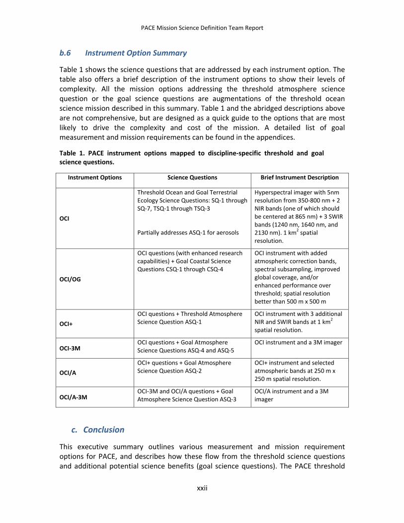
b.6 Instrument Option Summary
Table 1 shows the science questions that are addressed by each instrument option. The table also offers a brief description of the instrument options to show their levels of complexity. All the mission options addressing the threshold atmosphere science question or the goal science questions are augmentations of the threshold ocean science mission described in this summary. Table 1 and the abridged descriptions above are not comprehensive, but are designed as a quick guide to the options that are most likely to drive the complexity and cost of the mission. A detailed list of goal measurement and mission requirements can be found in the appendices.
Table 1. PACE instrument options mapped to discipline-specific threshold and goal science questions.
Instrument Options Science Questions Brief Instrument Description
OCI
Threshold Ocean and Goal Terrestrial Ecology Science Questions: SQ-1 through SQ-7, TSQ-1 through TSQ-3
Partially addresses ASQ-1 for aerosols
Hyperspectral imager with 5nm resolution from 350-800 nm + 2 NIR bands (one of which should be centered at 865 nm) + 3 SWIR bands (1240 nm, 1640 nm, and 2130 nm). 1 km2 spatial resolution.
OCI/OG
OCI questions (with enhanced research capabilities) + Goal Coastal Science Questions CSQ-1 through CSQ-4
OCI instrument with added atmospheric correction bands, spectral subsampling, improved global coverage, and/or enhanced performance over threshold; spatial resolution better than 500 m x 500 m
OCI+ OCI questions + Threshold Atmosphere Science Question ASQ-1
OCI instrument with 3 additional NIR and SWIR bands at 1 km2 spatial resolution.
OCI-3M OCI questions + Goal Atmosphere Science Questions ASQ-4 and ASQ-5
OCI instrument and a 3M imager
OCI/A OCI+ questions + Goal Atmosphere Science Question ASQ-2
OCI+ instrument and selected atmospheric bands at 250 m x 250 m spatial resolution.
OCI/A-3M OCI-3M and OCI/A questions + Goal Atmosphere Science Question ASQ-3
OCI/A instrument and a 3M imager
c. Conclusion
This executive summary outlines various measurement and mission requirement options for PACE, and describes how these flow from the threshold science questions and additional potential science benefits (goal science questions). The PACE threshold
xxii
PACE Mission Science Definition Team Report
ocean science mission will provide significant advancements in ocean ecology and biogeochemistry research. In essence, the hyperspectral capabilities of the OCI permit unprecedented global spectroscopy from space that will open many opportunities for Earth systems science research, yielding new discoveries and unique applications. The recommended stringent requirements for PACE ocean measurements will also ensure that the mission will provide the climate-quality data necessary to extend the historical ocean color record for understanding global ocean change and variability. Augmentations to OCI that address the goal ocean science questions would lead to refined understanding of global ocean biogeochemical processes, and to improved assessments of global coastal, estuarine, and inland aquatic habitats needed for resource management. These goals, and the requirements to address the atmosphere threshold and goal science questions, increase the complexity and cost of the mission. However, they would increase the value of the mission for global ocean science, coastal and inland water research, atmospheric science (through continuation of some legacy atmospheric measurements), and for an improved understanding of atmosphere-ocean interactions.
xxiii
PACE Mission Science Definition Team Report
Appendix I
Refer to section 3.2.11 for additional details.
Threshold Ocean Mission Requirements
Orbit • sun-synchronous polar orbit • equatorial crossing time between 11:00 and 1:00 • orbit maintenance to ±10 minutes over mission lifetime
Global Coverage • 2-day global coverage to solar zenith angle of 75o • mitigation of sun glint • multiple daily observations at high latitudes • view zenith angles not exceeding ±60o • mission lifetime of 5 years
Navigation and Registration
• pointing accuracy of 2 IFOV and knowledge equivalent to 0.1 IFOV over the full range of viewing geometries (e.g., scan and tilt angles)
• pointing jitter of less than 0.01 IFOV between any adjacent spatial samples • spatial band-to-band registration of 80% of one IFOV between any two bands, without resampling • simultaneity of 0.02 second (to ensure co-registration of spectral bands to within 80% of one IFOV
considering satellite along-track motion) Instrument Performance Tracking
• characterization of all detectors and optical components through monthly lunar observations through Earth-viewing port
• characterization of instrument performance changes to ±0.2% within the first 3 years and maintenance of this accuracy thereafter for the duration of the mission
• monthly characterization of instrument spectral drift to an accuracy of 0.3 nm • daily measurement of dark current and observations of a calibration target/source, with knowledge
of daily calibration source degradation to ~0.2% Instrument Artifacts
• Prelaunch characterization of linearity, response versus view angle (RVVA), polarization sensitivity, radiometric and spectral temperature sensitivity, high contrast resolution, saturation, saturation recovery, crosstalk, radiometric and band-to-band stability, onboard calibrator performance (e.g., bidirectional reflectance distribution of a diffuser, etc.), and relative spectral response
• prelaunch absolute calibration of 2% and on-orbit absolute calibration accuracy (before vicarious calibration) of better than 5%
• overall instrument artifact contribution to TOA radiance of <0.5% after correction • image striping to < 0.1% in calibrated TOA radiances • crosstalk contribution to radiance uncertainties 0.1% at Ltyp • polarization sensitivity of ≤1% and knowledge of polarization sensitivity to ≤ 0.2% • no detector saturation for any science measurement bands at Lmax • RVVA of <5% for the entire view angle range and by <0.5% for view angles that differ by less than 1o • Stray light contamination for the instrument < 0.2% of Ltyp 3 pixels away from a cloud • out-of-band contamination of <0.01 for all multispectral channels • radiance-to-counts relationship characterized to 0.1% over full dynamic range (from Ltyp to Lmax)
Spatial Resolution • Global spatial coverage of 1 km x 1 km (±0.1 km) along-track (nadir)
Atmospheric Corrections
• retrieval of [ρw(λ)]N for open-ocean, clear-water conditions and standard marine atmospheres with an accuracy of the maximum of either 5% or 0.001 over the wavelength range 400 – 710 nm
• Two NIR atmospheric correction bands (865 nm and either 820 or 940 nm) • NUV band centered near 350 nm • SWIR bands centered at 1240, 1640, and 2130 nm
Science Spectral Bands
• 5 nm spectral resolution from 350 to 800 nm • complete ground station downlink and archival of 5 nm data
Signal-to-noise • SNR at ocean Ltyp of 1000 from 360 to 800 nm; 300 @ 350 nm; 600 @ NIR bands; 250, 180, and 15 @ 1240, 1640, & 2130 nm
Mission • full reprocessing capability of all PACE data at a minimum frequency of 1 – 2 times annually • Integrated process studies, assessments, and cal/val studies • Three-hour data latency and direct broadcast of aggregate spectral bands • Robust data and results distribution system
xxiv
PACE Mission Science Definition Team Report
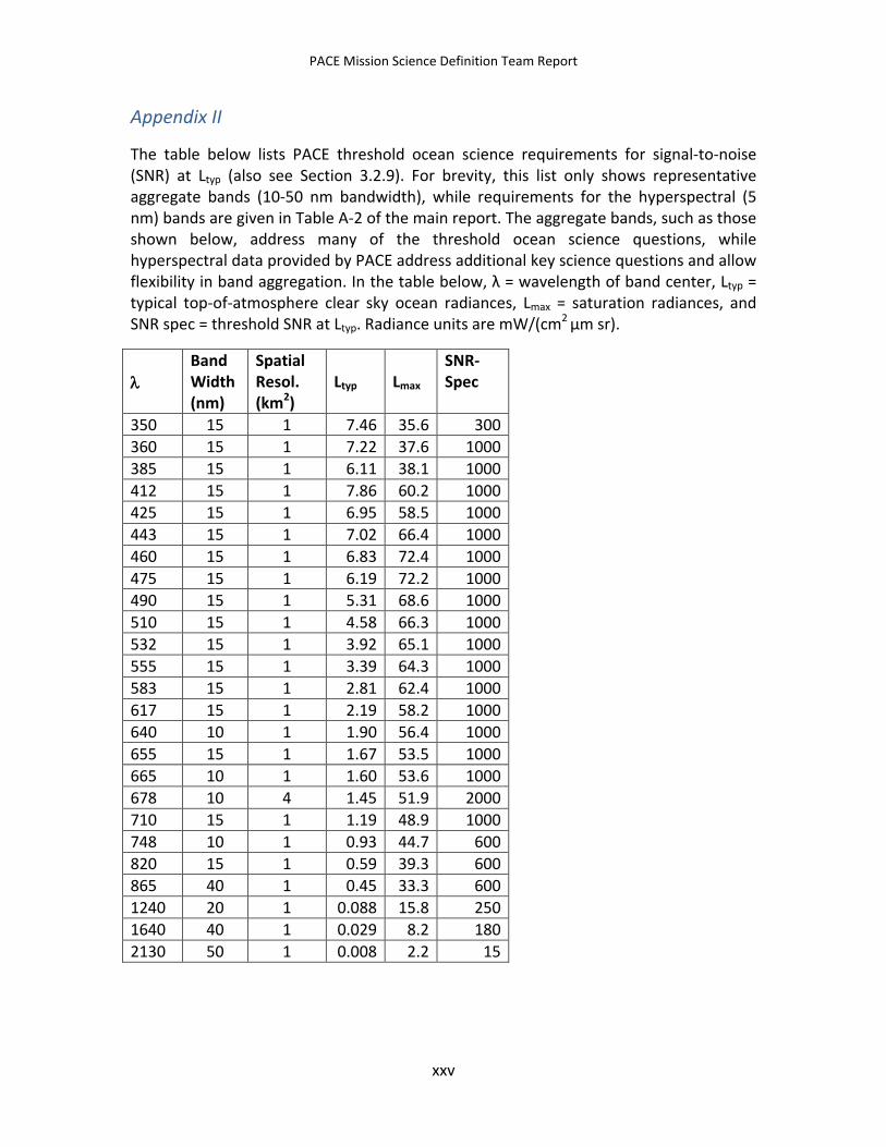
Appendix II
The table below lists PACE threshold ocean science requirements for signal-to-noise (SNR) at Ltyp (also see Section 3.2.9). For brevity, this list only shows representative aggregate bands (10-50 nm bandwidth), while requirements for the hyperspectral (5 nm) bands are given in Table A-2 of the main report. The aggregate bands, such as those shown below, address many of the threshold ocean science questions, while hyperspectral data provided by PACE address additional key science questions and allow flexibility in band aggregation. In the table below, λ = wavelength of band center, Ltyp = typical top-of-atmosphere clear sky ocean radiances, Lmax = saturation radiances, and SNR spec = threshold SNR at Ltyp. Radiance units are mW/(cm2 µm sr).
λ
Band Width (nm)
Spatial Resol. (km2)
Ltyp
Lmax
SNR- Spec
350 15 1 7.46 35.6 300 360 15 1 7.22 37.6 1000 385 15 1 6.11 38.1 1000 412 15 1 7.86 60.2 1000 425 15 1 6.95 58.5 1000 443 15 1 7.02 66.4 1000 460 15 1 6.83 72.4 1000 475 15 1 6.19 72.2 1000 490 15 1 5.31 68.6 1000 510 15 1 4.58 66.3 1000 532 15 1 3.92 65.1 1000 555 15 1 3.39 64.3 1000 583 15 1 2.81 62.4 1000 617 15 1 2.19 58.2 1000 640 10 1 1.90 56.4 1000 655 15 1 1.67 53.5 1000 665 10 1 1.60 53.6 1000 678 10 4 1.45 51.9 2000 710 15 1 1.19 48.9 1000 748 10 1 0.93 44.7 600 820 15 1 0.59 39.3 600 865 40 1 0.45 33.3 600 1240 20 1 0.088 15.8 250 1640 40 1 0.029 8.2 180 2130 50 1 0.008 2.2 15
xxv
PACE Mission Science Definition Team Report
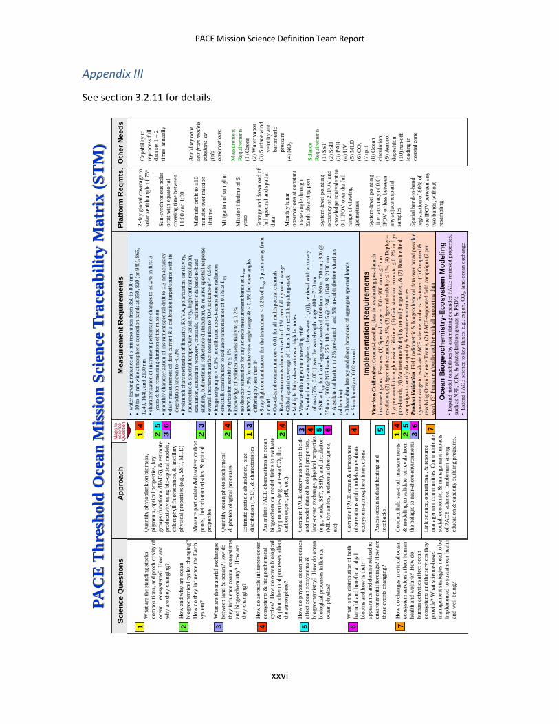
Appendix III
See section 3.2.11 for details. PA
CE
Thr
esho
ld O
cean
Mis
sion
Sci
ence
Tra
ceab
ility
Mat
rix
(ST
M)
Impl
emen
tatio
n R
equi
rem
ents
Vica
riou
s Cal
ibra
tion:
Gro
und-
base
d R
rsda
ta fo
r eva
luat
ing
post
-laun
ch
inst
rum
ent g
ains
. Fe
atur
es: (
1) S
pect
ral r
ange
= 3
50 -
900
nm a
t ≤ 3
nm
re
solu
tion,
(2) S
pect
ral a
ccur
acie
s ≤ 5
%, (
3) S
pect
ral s
tabi
lity
≤ 1%
, (4)
Dep
loy
= 1
yrpr
elau
nch
thro
ugh
mis
sion
life
time,
(5) G
ain
stan
dard
erro
rs to
≤ 0
.2%
in 1
yr
post
-laun
ch, (
6) M
aint
enan
ce &
dep
loy
cent
rally
org
aniz
ed, &
(7) R
outin
e fie
ld
cam
paig
ns to
ver
ify d
ata
qual
ity &
eva
luat
e un
certa
intie
sPr
oduc
t Val
idat
ion:
Fie
ld ra
diom
etric
& b
ioge
oche
mic
al d
ata
over
bro
ad p
ossi
ble
dyna
mic
rang
e to
eva
luat
e PA
CE
scie
nce
prod
ucts
. Fea
ture
s: (1
) Com
pete
d &
re
volv
ing
Oce
an S
cien
ce T
eam
s, (2
) PA
CE-
supp
orte
d fie
ld c
ampa
igns
(2 p
er
year
), (3
) Per
man
ent/p
ublic
arch
ive
with
all
supp
ortin
g da
ta
Oce
an B
ioge
oche
mis
try-
Ecos
yste
m M
odel
ing
•Exp
and
mod
el c
apab
ilitie
s by
assi
mila
ting
expa
nded
PA
CE
retri
eved
pro
perti
es,
such
as N
PP, I
OPs
, & p
hyto
plan
kton
gro
ups &
PSD
’s•
Exte
nd P
AC
E sc
ienc
e to
key
flux
es: e
.g.,
expo
rt, C
O2,
land
-oce
an e
xcha
nge
1 2 3 4 5 6
Wha
t are
the
stan
ding
stoc
ks,
com
posi
tions
, and
pro
duct
ivity
of
ocea
n
ecos
yste
ms?
How
and
w
hy a
re th
ey c
hang
ing?
How
and
why
are
oce
an
biog
eoch
emic
al c
ycle
s ch
angi
ng?
How
do
they
influ
ence
the
Earth
sy
stem
?
Wha
t are
the
mat
eria
l exc
hang
es
betw
een
land
& o
cean
? H
ow d
o th
ey in
fluen
ce c
oast
al e
cosy
stem
s an
d bi
ogeo
chem
istry
? H
ow a
re
they
cha
ngin
g?
How
do
aero
sols
influ
ence
oce
an
ecos
yste
ms
& b
ioge
oche
mic
al
cycl
es?
How
do
ocea
n bi
olog
ical
&
pho
toch
emic
al p
roce
sses
aff
ect
the
atm
osph
ere?
How
do
phys
ical
oce
an p
roce
sses
af
fect
oce
an ec
osys
tem
s &
bi
ogeo
chem
istry
? H
ow d
o oc
ean
biol
ogic
al p
roce
sses
influ
ence
oc
ean
phys
ics?
Wha
t is t
he d
istri
butio
n of
bot
h ha
rmfu
l and
ben
efic
ial a
lgal
bl
oom
s an
d ho
w is
thei
r ap
pear
ance
and
dem
ise
rela
ted
to
envi
ronm
enta
l for
cing
s? H
ow a
re
thes
e ev
ents
cha
ngin
g?
How
do
chan
ges i
n cr
itica
l oce
an
ecos
yste
m s
ervi
ces a
ffec
t hum
an
heal
th a
nd w
elfa
re?
How
do
hum
an a
ctiv
ities
aff
ect o
cean
ec
osys
tem
s an
d th
e se
rvic
es th
ey
prov
ide?
Wha
t sci
ence
-bas
ed
man
agem
ent s
trate
gies
nee
d to
be
impl
emen
ted
to su
stai
n ou
r hea
lth
and
wel
l-bei
ng?
7
Qua
ntify
phy
topl
ankt
on b
iom
ass,
pigm
ents
, opt
ical
pro
perti
es, k
ey
grou
ps (f
unct
iona
l/HA
BS)
, & e
stim
ate
prod
uctiv
ity u
sing
bio
-opt
ical
mod
els,
chlo
roph
yll f
luor
esce
nce,
& a
ncill
ary
phys
ical
pro
perti
es (e
.g.,
SST,
MLD
)
Mea
sure
par
ticul
ate &
diss
olve
d ca
rbon
po
ols,
thei
r cha
ract
eris
tics
& o
ptic
al
prop
ertie
s
Qua
ntify
oce
an p
hoto
bioc
hem
ical
&
pho
tobi
olog
ical
pro
cess
es
Estim
ate
parti
cle
abun
danc
e, s
ize
dist
ribut
ion
(PSD
), &
cha
ract
eris
tics
Ass
imila
te P
AC
E ob
serv
atio
ns in
oce
an
biog
eoch
emic
al m
odel
fiel
ds to
eva
luat
e ke
y pr
oper
ties (
e.g.
, air-
sea
CO
2flu
x,
carb
on ex
port,
pH
, etc
.)
Com
pare
PA
CE
obse
rvat
ions
with
fiel
d-an
d m
odel
dat
a of
bio
logi
cal p
rope
rties
, la
nd-o
cean
exch
ange
, phy
sica
l pro
perti
es
(e.g
., w
inds
, SST
, SSH
), an
d ci
rcul
atio
n (M
L dy
nam
ics,
horiz
onta
l div
erge
nce,
et
c)
Com
bine
PA
CE
ocea
n &
atm
osph
ere
obse
rvat
ions
with
mod
els t
o ev
alua
te
ecos
yste
m-a
tmos
pher
e in
tera
ctio
ns
Ass
ess
ocea
n ra
dian
t hea
ting
and
feed
back
s
Con
duct
fiel
d se
a-tru
th m
easu
rem
ents
&
mod
elin
g to
val
idat
e re
triev
als f
rom
th
e pe
lagi
c to
nea
r-sho
re e
nviro
nmen
ts
Link
scie
nce,
ope
ratio
nal,
& re
sour
ce
man
agem
ent c
omm
uniti
es. C
omm
unic
ate
soci
al, e
cono
mic
, & m
anag
emen
t im
pact
s of
PA
CE
scie
nce.
Im
plem
ent s
trong
ed
ucat
ion
& c
apac
ity b
uild
ing
prog
ram
s.
1 2 2 22
3 33 44 4 4 5553
46
1 2 3
4 5 66 7
1
2-da
y gl
obal
cov
erag
e to
so
lar z
enith
ang
le o
f 75o
Sun-
sync
hron
ous p
olar
or
bit w
ith e
quat
oria
l cr
ossi
ng ti
me
betw
een
11:0
0 an
d 1:
00
Mai
ntai
n or
bit t
o ±1
0 m
inut
es o
ver m
issi
on
lifet
ime
Miti
gatio
n of
sun
glin
t
Mis
sion
life
time
of 5
ye
ars
Stor
age
and
dow
nloa
d of
fu
ll sp
ectra
l and
spat
ial
data
Mon
thly
luna
r ob
serv
atio
ns a
t con
stan
t ph
ase
angl
e th
roug
h Ea
rth o
bser
ving
por
t
Syst
em-le
vel p
oint
ing
accu
racy
of 2
IFO
V a
nd
know
ledg
e eq
uiva
lent
to
0.1
IFO
V o
ver t
he fu
ll ra
nge
of v
iew
ing
geom
etrie
s
Syst
em-le
vel p
oint
ing
jitte
r acc
urac
y of
0.0
1 IF
OV
or l
ess b
etw
een
any
adja
cent
spat
ial
sam
ples
Spat
ial b
and-
to-b
and
regi
stra
tion
of 8
0% o
f on
e IF
OV
bet
wee
n an
y tw
o ba
nds,
with
out
resa
mpl
ing
Cap
abili
ty to
re
proc
ess f
ull
data
set 1
–2
times
ann
ually
Anci
llary
dat
a se
ts fr
om m
odel
s m
issi
ons,
or
field
ob
serv
atio
ns:
Mea
sure
men
tR
equi
rem
ents
(1) O
zone
(2) W
ater
vap
or(3
) Sur
face
win
dve
loci
ty a
ndba
rom
etric
pres
sure
(4) N
O2
Scie
nce
Req
uire
men
ts(1
) SST
(2) S
SH(3
) PA
R(4
) UV
(5) M
LD(6
) CO
2(7
) pH
(8) O
cean
ci
rcul
atio
n(9
) Aer
osol
de
posi
tion
(10)
run-
off
load
ing
in
coas
tal z
one
•w
ater
leav
ing
radi
ance
at 5
nm
reso
lutio
n fro
m35
0to
800
nm
•10
to 4
0 nm
wid
e at
mos
pher
ic co
rrec
tion
band
s at 3
50, 8
20 (o
r 940
), 86
5,
1240
, 164
0, an
d 21
30 n
m•c
hara
cter
izat
ion
of in
stru
men
t per
form
ance
cha
nges
to ±
0.2%
in fi
rst 3
year
s & fo
r rem
aini
ng d
urat
ion
of th
e m
issi
on•m
onth
ly c
hara
cter
izat
ion
of in
stru
men
t spe
ctra
l drif
t to
0.3
nm a
ccur
acy
•dai
ly m
easu
rem
ent o
f dar
k cu
rren
t & a
cal
ibra
tion
targ
et/s
ourc
e with
its
degr
adat
ion
know
n to
~0.
2%•P
rela
unch
char
acte
rizat
ion
of li
near
ity, R
VV
A, p
olar
izat
ion
sens
itivi
ty,
radi
omet
ric &
spec
tral t
empe
ratu
re se
nsiti
vity
, hig
h co
ntra
st re
solu
tion,
satu
ratio
n, sa
tura
tion
reco
very
, cro
ssta
lk, r
adio
met
ric &
ban
d-to
-ban
dst
abili
ty, b
idire
ctio
nal r
efle
ctan
ce d
istri
butio
n, &
rela
tive
spec
tral r
espo
nse
•ove
rall
inst
rum
ent a
rtifa
ct c
ontri
butio
n to
TO
A ra
dian
ce o
f < 0
.5%
•im
age
strip
ing
to <
0.1
% in
cal
ibra
ted
top-
of-a
tmos
pher
e ra
dian
ces
•cro
ssta
lk c
ontri
butio
n to
radi
ance
unc
erta
intie
s of 0
.1%
at L
typ
•pol
ariz
atio
n se
nsiti
vity
≤ 1
%•k
now
ledg
e of
pol
ariz
atio
n se
nsiti
vity
to ≤
0.2
%•n
o de
tect
or sa
tura
tion
for a
ny sc
ienc
e m
easu
rem
ent b
ands
at L
max
•RV
VA
of <
5%
for e
ntire
vie
w a
ngle
rang
e &
< 0
.5%
for v
iew
ang
les
diffe
ring
by le
ss th
an 1
o
•Stra
y lig
ht c
onta
min
atio
n fo
r the
inst
rum
ent <
0.2
% o
f Lty
p3
pixe
ls aw
ay fr
om
a cl
oud
•Out
-of-b
and
cont
amin
atio
n <
0.01
for a
ll m
ultis
pect
ral c
hann
els
•Rad
ianc
e-to
-cou
nts c
hara
cter
ized
to 0
.1%
ove
r ful
l dyn
amic
rang
e •G
loba
l spa
tial c
over
age
of 1
km
x 1
km
(±0.
1 km
) alo
ng-tr
ack
•Mul
tiple
dai
ly o
bser
vatio
ns at
hig
h la
titud
es•V
iew
zen
ith an
gles
not
exc
eedi
ng ±
60o
•St
anda
rd m
arin
e at
mos
pher
e, cl
ear-w
ater
[rw(
l)]N
retri
eval
with
acc
urac
yof
max
[5%
, 0.
001]
ove
r the
wav
elen
gth
rang
e 40
0 –
710
nm•
SNR
at L
typ
for 1
km
2ag
greg
ate
band
s of 1
000
from
360
to 7
10 n
m; 3
00 @
35
0 nm
; 600
@ N
IR b
ands
; 250
, 180
, and
15
@ 1
240,
164
0, &
213
0 nm
•A
bsol
ute
calib
ratio
n to
2%
pre
-laun
ch a
nd 5
% o
n-or
bit (
befo
re v
icar
ious
ca
libra
tion)
•3 h
our d
ata
late
ncy
and
dire
ct b
road
cast
of a
ggre
gate
spec
tral b
ands
•Si
mul
tane
ity o
f 0.0
2 se
cond
Map
s to
Sci
ence
Que
stio
nSc
ienc
e Q
uest
ions
A
ppro
ach
M
easu
rem
ent R
equi
rem
ents
Pl
atfo
rm R
eqm
ts.
Oth
er N
eeds
xxvi
PACE Mission Science Definition Team Report
Appendix IV
The following is a list of additional PACE ocean science measurement goals beyond the threshold requirements (see Section 3.2.12). These goals are listed in alphabetical order according to topic (italics) and thus are not listed according to priority. These goals do not represent a trade space with threshold requirements, but are beneficial to the mission if achieved in addition to the threshold mission requirements described in Appendices I and II.
• Accuracy: Retrieval of normalized [ρw(λ)]N for open-ocean, clear-water conditions and standard marine atmospheres with an accuracy of the maximum of either 10% or 0.002 over the wavelength range of 350 – 395 nm
• Aerosol heights: Identified approach or measurement capacity for evaluating/measuring aerosol vertical distributions and type for improved atmospheric corrections.
• Atmospheric correction: SWIR atmospheric correction band at 2130 nm with a SNR of 100.
• Coverage: 1-day global coverage
• Coverage: Coverage to a solar zenith angle >75o
• Crossing time: Noon equatorial crossing time (±10 min)
• Data Latency: 0.5 hour data latency and direct broadcast of 5 nm resolution data
• Instrument artifact: Overall instrument artifact contribution to top of the atmosphere (TOA) radiance retrievals of <0.2%.
• Navigation and Registration: pointing knowledge of 0.05 Instantaneous Field of View (IFOV); band-to-band registration of 90% of one IFOV; simultaneity of 0.01 second
• Nitrogen dioxide: Identified approach for characterizing NO2 and ozone concentrations at sufficient accuracy for improving atmospheric corrections
• Mission lifetime: 10 years
• Performance changes: Characterization of instrument performance changes to ±0.1% within 3 years and maintenance of this accuracy thereafter
• Saturation: No detector saturation for any science measurement bands up to 1.2 × Lmax
• Signal-to-noise: SNR for bio-optical science bands and/or atmospheric correction bands greater than those shown in Appendix II
xxvii
PACE Mission Science Definition Team Report
• Spatial resolution: Spatial resolution of 1 km2 (±10%) at all angles across track
• Spatial resolution: Along-track spatial resolution of 250 m x 250 m to <1 km2 for inland, estuarine, coastal, and shelf area retrievals for all bands or a subset of bands
• Spectral coverage: 5 nm spectral coverage from 800 to 900 nm
• Spectral sub-sampling: Spectral sub-sampling at ~1-2 nm resolution from 655 to 710 nm for refined characterization of the chlorophyll fluorescence spectrum
xxviii
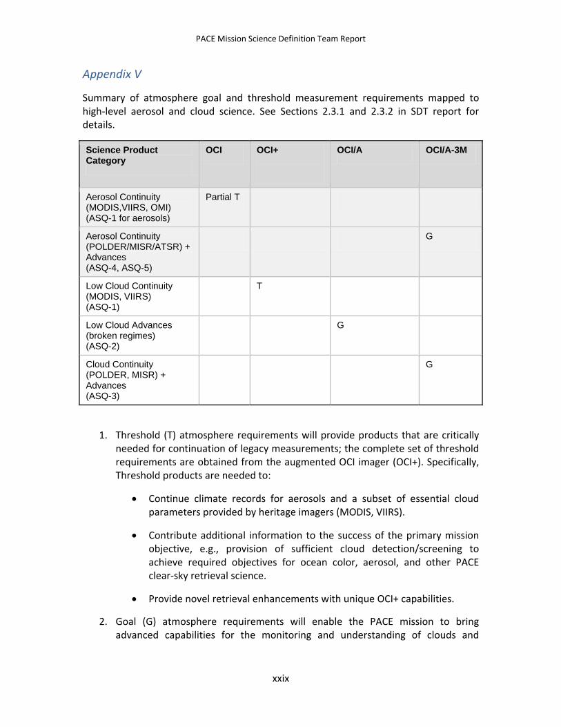
PACE Mission Science Definition Team Report
Appendix V
Summary of atmosphere goal and threshold measurement requirements mapped to high-level aerosol and cloud science. See Sections 2.3.1 and 2.3.2 in SDT report for details.
Science Product Category
OCI OCI+
OCI/A OCI/A-3M
Aerosol Continuity (MODIS,VIIRS, OMI) (ASQ-1 for aerosols)
Partial T
Aerosol Continuity (POLDER/MISR/ATSR) + Advances (ASQ-4, ASQ-5)
G
Low Cloud Continuity (MODIS, VIIRS) (ASQ-1)
T
Low Cloud Advances (broken regimes) (ASQ-2)
G
Cloud Continuity (POLDER, MISR) + Advances (ASQ-3)
G
1. Threshold (T) atmosphere requirements will provide products that are critically needed for continuation of legacy measurements; the complete set of threshold requirements are obtained from the augmented OCI imager (OCI+). Specifically, Threshold products are needed to:
• Continue climate records for aerosols and a subset of essential cloud parameters provided by heritage imagers (MODIS, VIIRS).
• Contribute additional information to the success of the primary mission objective, e.g., provision of sufficient cloud detection/screening to achieve required objectives for ocean color, aerosol, and other PACE clear-sky retrieval science.
• Provide novel retrieval enhancements with unique OCI+ capabilities.
2. Goal (G) atmosphere requirements will enable the PACE mission to bring advanced capabilities for the monitoring and understanding of clouds and
xxix
PACE Mission Science Definition Team Report
aerosols, and will be linked to OCI/A or OCI/A-3M instrument observations (i.e., higher spatial resolution OCI+ and 3MI-like). Goal products will:
• Complement time series of advanced cloud and aerosol variables observed by heritage sensors (POLDER, Multiangle Imaging SpectroRadiometer [MISR]).
• Contribute to the advance of cloud research through provision of higher spatial resolution and/or new or enhanced cloud parameters from spectral capabilities not currently available from any existing or past mission.
The table below contains a summary of cloud and aerosol augmentations to the baseline (ocean science threshold) OCI imager specifications, categorized according to threshold and goal atmosphere measurement requirements. Refer to Section 3.3.11 and Appendix B for further details.
xxx
PACE Mission Science Definition Team Report
Augmentation to baseline OCI (i.e., Threshold ocean requirements from Section 3.2)
Central Wave-length (µm)
Band-width
(FWHM, nm)
Rmax a (µ0=1)
Lmax a (W/m2-sr-µm)
Rtyp a,b (µ0=1)
Ltyp b (W/m2-sr-µm)
NEdR@Rtyp
SNR@Ltyp a
Spatial Resolution (m)
[Threshold, Goal c]
0.940 25 0.80 210 0.03 7.8 0.0002 150 1000
1.378 10 d 0.80 95 0.03 3.5 0.0003 100 1000
2.250 e 50 0.90 21 0.03 0.7 0.0002 150 1000
250
Additional info. and/or modification to OCI
0.665 as for OCI
aggreg.
1000
250
0.865 as for OCI
1000
250
1.640 as for OCI
1000
250
2.135 as for OCI
1000
250
0.763f 5nm; CW tolerance: ±2.5nm; BW/CW knowledge: < 0.1 nm
1000
250
Table notes:
a. Generally consistent with MODIS 0.94 and 1.38 µm 1 km native resolution bands and VIIRS 2.25 µm channel at nadir native resolution. When referenced to above OCI Ltyps, MODIS SNRs in the 1 km 0.94 and 1.38 µm bands are 130 and 90, respectively. At above Ltyp, VIIRS 2.25 µm band SNR is ~60. For MODIS, Rsat ~15% larger than Rmax in these bands.
b. Rtyp corresponds to cirrus optical thickness of approximately 0.2–0.3.
c. Goal spatial resolution for reduction of low cloud heterogeneity biases.
xxxi
PACE Mission Science Definition Team Report
d. Goal BW (MODIS 30 nm BW found to be too large for adequate cirrus detection; VIIRS 15 nm found to be significantly better).
e. For cloud phase and VIIRS/ABI cloud microphysics continuity.
f. POLDER and Medium-spectral Resolution Imaging Spectrometer (MERIS) cloud pressure height heritage.
xxxii
PACE Mission Science Definition Team Report
1 Introduction
1.1 The Science of PACE The oceans are an integral part of the Earth system and provide important goods and services to our society. The ocean ecosystem is being affected simultaneously by climate variability and increasing human demands. To understand and respond to these challenges, scientists and policy makers need to continue current ocean measurement efforts and develop new, advanced measuring and monitoring capabilities. The Pre-Aerosol, Clouds, and ocean Ecosystem (PACE) mission will make global ocean color measurements that are essential for understanding the global carbon cycle and its interrelationship with climate change. New and continuing observations of ocean ecology and biogeochemistry are required to quantify aquatic carbon storage and ecosystem function in response to human activities and natural events. A key PACE objective is the improvement of climate-carbon and climate-ecology model prediction. The PACE mission will also ensure the continuation of ocean color data records that are needed to differentiate natural variability from anthropogenic climate change. Consequently, the primary sensor on PACE is an ocean color imager (OCI) designed to collect global ocean color observations that address key interrelated ocean biology and biogeochemistry science questions.
The emphasis of PACE is ocean ecology and biogeochemistry, but the 2010 NASA plan for Earth observations that introduced the PACE mission4 specified a capability to “extend data records on aerosols and clouds” from heritage sensors and cited specific instruments5 to provide context for the PACE mission. The original scope of the PACE SDT also included the Centre National d'Études Spatiales (CNES) “3M Imager” (3MI) instrument concept being proposed for the Eumetsat Polar System–Second Generation (EPS-SG) system. However, in March 2012, the European Space Agency (ESA) decided to support 3MI on EPS-SG, and not to contribute a polarimeter for PACE. Nevertheless, the SDT addressed the science capabilities of a 3MI-like instrument: (1) because such an instrument would be useful for aerosol, cloud, and ocean science, and (2) to provide NASA with science and measurement requirements in case the PACE mission budget could grow to accommodate this type of sensor.
1.2 The PACE Science Definition Team Philosophy and Methods In autumn of 2011, NASA convened a science definition team (SDT) to provide the science justification and measurement and mission requirements for the PACE mission. The SDT included experts in ocean and atmospheric remote sensing, and instrument design who relied on experience, technical reports, SDT studies, and the assistance of a
4 “Responding to the Challenge of Climate and Environmental Change: NASA’s Plan for a Climate-Centric Architecture for Earth Observations and Applications from Space, June 2010.” 5 Spectral scanning and multi-angle imagers (MODIS and MISR, respectively), and Multi-directional, Multi-polarization and Multispectral (3M) imaging sensors (e.g. POLDER).
1
PACE Mission Science Definition Team Report
NASA engineering team (ET) to produce this report. The PACE SDT was thoughtful about budget limitations and used two Instrument Design Lab (IDL) studies and one Mission Design Lab (MDL) study provided by the ET to understand budgetary impacts of various mission options. The SDT met three times during 2011–2012, held teleconferences nearly every week, and sustained extensive communication between its members and the community at large.
1.3 Structure of the Report This report presents the scientific justification for the PACE mission. Although the emphasis of PACE is ocean ecology and biogeochemistry, this SDT concluded that various fields of research may benefit from this mission. Accordingly, the science justification of PACE is divided by its contribution to the fields of Ocean Ecology and Biogeochemistry (section 2.2), Atmosphere (section 2.3), Terrestrial Ecology (section 2.4), and Watersheds and Lakes (section 2.5). Decades of experience working with global satellite missions have demonstrated that achieving research-quality ocean color data requires more than just high quality sensors. Based on this experience, the SDT embraced a ‘whole mission concept’ that encompasses continual post-launch sensor calibration, processing and reprocessing of satellite data, algorithm development and maintenance, and field validation of data products. The mission concept should also include a robust data and product distribution system and process studies and synthesis efforts to advance knowledge about the science questions6. All of these activities must be viewed as integral to the PACE mission and included in flight project planning. Pre-launch and post-launch process studies supporting the central remote sensing measurements are required to fully address the science questions presented in this SDT report. Accordingly, this report follows the science justification with a comprehensive discussion on science-driven measurement requirements (section 3) also parsed by science discipline. The report also covers mission requirements needed to sustain the production of research quality data (section 4). Finally, section 5 of this report addresses the possible synergies between PACE and other programs with emphasis in the use of PACE for applications. The SDT concluded that ocean threshold and goal requirements and atmosphere threshold and goal requirements are best addressed with very distinct instrument and mission options. In section 6 we present a menu of instrument options that would address specific combinations of threshold and goal science requirements.
Throughout this report, science questions, measurement requirements, and mission requirements were separated into two categories, namely ‘threshold’ and ‘goal’:
• Threshold science questions (as defined in section 2.2.1 and section 2.3) encompass the required, highest-priority research that defines the PACE mission. Threshold measurement and mission requirements are those that are imperatives to answering the threshold science questions.
6 Assessing Requirements for sustained Ocean Color Research and Operations. 2011. National Research Council, National Academies Press, http://www.nap.edu/catalog.php?record_id=13127.
2
PACE Mission Science Definition Team Report
• Goal science questions (as defined in Section 2.2.2.12, Section 2.3, and Section 2.4.1) describe additional science research that the PACE mission could potentially accomplish. Goal measurement and mission requirements add value to the mission by increasing the quality and quantity of the retrieval information. Goal measurement and mission requirements can enable research regarding the goal science questions or permit enhanced research concerning threshold and goal science questions. Goals increase the number of data products (including atmospheric and terrestrial parameters) from the mission and enhance the value of PACE data for science and applications. However, the SDT emphasizes throughout this document that achieving goal requirements cannot compromise any of the threshold requirements.
This report also presents additional, independent requirements for continuing aerosol data records and a subset of cloud data records, and discusses advantages and requirements of a co-manifested 3M-like instrument. However, the emphasis of PACE is ocean ecology and biogeochemistry and not attaining requirements for threshold (heritage) atmospheric products should not jeopardize the threshold ocean science objectives of the PACE mission.
Finally, in sections 3 and 4 of this report the SDT tried to strike a balance between prescribing very specific measurement and mission requirements and leaving solutions open for novel technology approaches to be proposed by the community. However, when the SDT has prescribed specific approaches, it has done so based on three decades of experience in making high quality ocean measurements from multiple orbital, sub-orbital, and field platforms. The SDT believes that ignoring these requirements will imperil the quality of the PACE science data.
3
PACE Mission Science Definition Team Report
2 Scientific Objectives
2.1 Introduction The PACE mission was conceived to provide new information for understanding the living ocean. PACE will make global ocean color measurements that are essential for understanding the carbon cycle and its interrelationship with climate change, and will expand our understanding about ocean ecology and biogeochemistry. The PACE mission can also make significant contributions to atmospheric, terrestrial, inland waters (e.g., Great Lakes), and watershed research. Section 2 of this report provides the scientific justification for the PACE mission in these areas, with emphasis on the threshold ocean ecology and biogeochemistry science questions that drive the PACE mission.
2.2 Ocean Ecosystems and Biogeochemistry For over thirty years, NASA’s satellite ocean color sensor data have enabled profound discoveries regarding global ocean biology and biogeochemistry. From the proof-of-concept Coastal Zone Color Scanner (CZCS: 1978-1986) to the Sea-Viewing Wide Field of View Sensor (SeaWiFS: 1997-2010) and the Moderate Resolution Imaging Spectroradiometer (MODIS: 2002-present), these sensors have enabled the exploration of Earth’s living ocean, a heritage to which the Visible Infrared Imager Radiometer Suite (VIIRS) now contributes. These global ocean sensors have documented a constantly changing Earth system in which natural and human factors interplay. Satellite ocean observations provide the ‘wide-angle lens’ with which to view the vast expanses of ocean surface ecosystems—a perspective beyond the reach of even the most ambitious field campaigns. Yet these missions are recent, so only a very brief record currently exists regarding global changes in ocean biogeochemistry. Nevertheless, observations from the heritage missions have greatly improved our understanding of the oceans and their relevance to human health and economic well-being.
The success of past ocean color missions is due not only to exceptional satellite instruments, but also to rigorous mission calibration/validation programs, repeated data reprocessing, and supporting ground-based research by the science community. Of critical importance are scientific synthesis efforts that include focused and broad-scope process and modeling studies integrated with the mission concept. All of these activities are integral to and essential for a successful ocean color mission. As detailed in this report, PACE ocean science objectives far exceed those of our heritage ocean color missions, resolving outstanding issues currently impeding scientific advancements and reflecting a community vision that has been in maturation for over a decade. Accordingly, the PACE mission relies even more critically on an end-to-end partnership of satellite remote sensing, in-water campaigns (e.g., ship, mooring, and drifter), global system modeling, and science synthesis efforts. We live in an era of rapidly changing climate and a rapidly growing human population is increasingly taxing our natural
4
PACE Mission Science Definition Team Report
marine resources. The PACE mission will provide invaluable new information for understanding ocean ecosystem and carbon cycle change and for improving forecasts of Earth system variability.
While the SeaWiFS and MODIS missions addressed major deficiencies in the proof-of-concept CZCS design (e.g., additional near infrared [NIR] atmospheric correction bands, mission-long on-orbit and field calibration programs), the ocean measurement requirements for both sensors reflect the state-of-the-science in the 1980s, focusing on a limited set of ocean properties (e.g., chlorophyll concentration and [MODIS only] fluorescence). While continuing these observations is essential to long-term climate data records, such observations are far from sufficient for today’s needs. From advances in ocean optics and marine ecology, we have now come to understand that even the interpretation of global trends in chlorophyll and their implications on ocean productivity and carbon cycling are far from straightforward. Their understanding requires accurate separation of independently varying, optically active, in-water constituents; characterization of phytoplankton physiological changes; and separation of specific nutritional constraints. Changes in Earth’s climate system and ocean physics (e.g., mixed layer seasonal cycles) and chemistry (e.g., acidification, nutrient balance) are altering ecological niches, impacting plankton community composition, seasonal succession, and threatening specific phytoplankton functional groups (e.g., coccolithophorids). The importance of atmosphere-ocean biology interactions is also becoming increasingly clear, including nutrient and toxin deposition on ecosystem health and ocean emissions on cloud formation and physics. Major advances have also been realized in prognostic Earth system modeling, but a range of global ocean carbon cycle properties (not only chlorophyll) are needed for model evaluation. Conversely, the coordination of satellite ocean products with central model parameters allows extension of observations to key carbon cycle processes that are multiple steps removed from ocean optics, such as the flux of carbon exported from the ocean surface layer to the deep sea, a key process in atmospheric CO2 dynamics.
Reflecting the growing needs for advanced ocean color remote sensing capabilities, seven overarching science questions are identified for the PACE mission. These questions lead to a specific set of targeted geophysical property retrievals, each linked directly to spectral reflectance features or derived from a combination of observables or satellite-field-model properties. The comprehensive PACE mission defined here builds upon lessons learned from heritage missions, addresses major new science needs through demonstrated approaches, entails essential field and modeling components, and enables unforeseen science advances. The PACE mission will provide the enriched observations necessary for the accurate interpretation of the long-term ocean climate data record and, in this manner alone, will make important contributions toward our understanding of the Earth system. PACE may further serve as a pathfinder for the future Aerosol/Cloud/Ecosystems (ACE) mission or function as the blueprint for generations of ocean color missions to come. In all cases, PACE will advance NASA’s ocean color remote sensing capabilities to reflect the maturity of contemporary ocean
5
PACE Mission Science Definition Team Report
science, addressing societal needs and creating a foundation for discovery for the next generation of scientists exploring Earth’s living oceans.
2.2.1 Threshold Ocean Science Questions
2.2.1.1 Ecosystem Properties and Change Marine ecosystems are complex entities encompassing vast numbers of species functioning over a wide range of space and time scales. Our understanding of links between biodiversity, ecosystem structure, and ecological function is incomplete, as is our grasp of how these linkages and processes vary over space and time. With our current observational and modeling tools, we have only begun to constrain estimates of the flow and cycling of carbon and other life-elements within and between ecosystems or the impact of climate and other physical and chemical environmental changes on ecological systems. However, from this work, clear paths have emerged for accelerating our characterization and understanding of ocean ecosystems. These paths require a significant advancement in satellite ocean color spectral resolution and spectral range. Improved spatial resolution is also advantageous for inland, estuarine, coastal, and shelf areas, which in the aggregate have significant implications on global biogeochemistry and are particularly relevant to living marine resources and sustained ecosystem services. The PACE sensor and mission requirements defined in this document address these requisite advances, allowing quantification of phytoplankton biomass, pigments and optical properties; assessment of key phytoplankton groups; characterization of ocean particle abundances, properties, and size distributions; and evaluation of local-to-global scale productivity and physiological status. With these capabilities, PACE will contribute greatly toward answering the science questions (SQ):
SQ-1: What are the standing stocks, compositions, and productivity of ocean ecosystems? How and why are they changing?
2.2.1.2 Ecosystems within the Earth System The very nature of our Earth system is indelibly marked by the signatures of life. This link between the physical-chemical properties of our planet and its occupants began nearly 4 billion years ago and is perhaps even more prevalent today than at any other time in history. Biochemical processes acting at the subcellular level are integrated across innumerable organisms to achieve truly global expressions that affect Earth system energy flow, chemistry, and climate. The ceaseless activities of ocean life profoundly impact the biogeochemical cycling of carbon, nitrogen, phosphorous, and other nutrients, as well as interact with and modify the overlying atmosphere (e.g., carbon dioxide and aerosol loads). Yet, despite its long and important history and the myriad links between ocean biology and the greater Earth system, our understanding of the underlying processes and their limitations remains rudimentary and we are easily caught off-guard by unanticipated feedbacks. An improved ability to characterize the role of ocean biology on global elemental cycles and forecast change can be achieved by
6
PACE Mission Science Definition Team Report
integrating global data on phytoplankton biomass, productivity, and functional groups; particulate and dissolved carbon pools; and particle size distributions into ocean biogeochemical models. Using conceptual models and numerical simulations, export of Particulate Organic Carbon (POC) into the deep ocean and air-sea fluxes of CO2, O2 and other important trace gases can be evaluated. The expanded suite of geophysical properties retrieved by PACE fulfills this need to address the questions:
SQ-2: How and why are ocean biogeochemical cycles changing? How do they influence the Earth system?
2.2.1.3 The Critical Coastal Zone One of the most vulnerable ocean habitats and valuable resources is the coastal zone, which constitutes an area of intense human growth (over one quarter of the human population and nearly half of the U.S. population) and commercial activity. The coastal zone extends across estuaries and the continental shelf and is the recipient of immense material loads from land. When integrated over its entirety, this region is responsible for 10% to 15% of global ocean primary productivity. Of all ocean environments, the coastal zone is most closely linked to changing human activities and is a region of extremes in productivity, carbon deposition, eutrophication, and elemental cycling. These processes sometimes lead to the formation of anoxic conditions and associated fish kills, directly impacting local economies. Coastal zones are notoriously challenging to characterize optically, due to the influence of land and underlying sediments. Therefore, they require spectral and spatial resolutions beyond those of heritage ocean color sensors. Coastal zone research and studies of inland water bodies can also benefit from improvements in spatial resolution over heritage ocean color sensors. The expanded observational capabilities of PACE will enable advanced retrievals of coastal zone particle abundances and properties, phytoplankton pigment loads and dominant functional groups, and dissolved material concentrations, characteristics, and optical properties. With these developments, major advances can be made in answering the questions:
SQ-3: What are the material exchanges between land and ocean? How do they influence coastal ecosystems and biogeochemistry? How are they changing?
2.2.1.4 Ocean – Atmosphere Interactions The atmosphere and ocean are intimately linked through the exchange of gases and aerosols across the interface. Ocean ecology and atmospheric aerosols encompass a unified and interdependent system, involving deposition of aerosols into the ocean and release of biological byproducts into the atmosphere. These feedbacks are tightly coupled to the Earth’s climate, and indeed biogeochemical and anthropogenic impacts on aerosol indirect effects remain major uncertainties in climate change forecasts. Ocean biology also has significant effects on atmospheric composition, including air-sea
7
PACE Mission Science Definition Team Report
carbon dioxide fluxes through phytoplankton photosynthesis and vertical carbon export, and release of aerosols, such as sulfate particle enrichment through dimethyl sulfide production. Combining dynamic aerosol modeling with PACE observations will contribute toward a further understanding of these interactions, providing insights on the questions:
SQ-4: How do aerosols influence ocean ecosystems and biogeochemical cycles? How do ocean biological and photochemical processes affect the atmosphere?
Within the ocean-atmosphere interactions umbrella of SQ-4 is the climate-relevant issue of atmospheric iron deposition on surface ocean biology. Iron availability in the ocean surface layer is an indisputable factor governing ecosystem composition and functionality. Despite its importance over contemporary and geologic time scales, this interaction is complex and difficult to characterize globally, since it is dependent on dust source, atmospheric chemistry, transport time, and physiological status of the receiving ocean ecosystem. One of the ‘goal’ instrumentation options for PACE that is described in this document is the inclusion of Multi-directional, Multi-polarization and Multispectral (3M) measurements, including SWIR spectral channels similar to the European 3MI. If this option is supported, it would enable unique capabilities for detecting coarse mode dust aerosols and important optical properties (optical depth, complex index of refraction, height information) that provide significant information on iron fertilization of key ocean regions, such as the Southern Ocean, equatorial Pacific, and subarctic Pacific. These detailed evaluations would not be possible with the PACE ocean radiometer alone. The additional 3M measurements will provide the greatest insights on atmospheric iron deposition impacts when coupled to an aerosol data assimilation system (see section 2.3).
2.2.1.5 Links between Ocean Biology and Physics NASA’s ocean color remote sensing programs have provided an unprecedented view of surface phytoplankton pigment concentration at the global scale and striking illustrations of first-order dependencies of ocean biology on physical forcings. Moreover, analyses of the full satellite record demonstrate that temporal changes in ocean biology from interannual to decadal scales can be traced directly to dominant modes of variability in physical properties. Feedbacks also exist between ocean biology and physics through, for example, changes in solar heating of the ocean surface by light absorption of phytoplankton pigment and colored dissolved organic materials. Understanding these interactions requires coupling ocean physics models with remote sensing measurements that allow more accurate separation and characterization of upper ocean particle assemblages and chemistry than achieved with heritage ocean color sensors. With these improved products, it will be possible to correctly assign mechanistic underpinnings to observed temporal shifts in biological properties, such as
8
PACE Mission Science Definition Team Report
distinguishing biomass, growth rate, and light acclimation contributions to the observed inverse relationship between global surface layer chlorophyll levels and sea surface temperature. With the advanced observational capabilities of the PACE mission, greater insights will be gained on answers to the questions:
SQ-5: How do physical ocean processes affect ocean ecosystems and biogeochemistry? How do ocean biological processes influence ocean physics?
2.2.1.6 Biological Events in the Ocean Phytoplankton blooms are important features to natural systems and to humans. For example in many open and coastal ocean settings, seasonal blooms—i.e., elevated biomass—sustain massive fisheries; are responsible for major migrations in birds, marine mammals, and pelagic fishes; and are associated with an enormous drawdown of atmospheric carbon dioxide. In near-shore, estuarine, and shelf habitats, phytoplankton blooms can also lead to strong anoxia and fish die-offs or be associated with toxic or otherwise harmful species. The mechanisms responsible for blooms and their associated species are far from understood, but in all cases it is clear that nutrients, light, and predator-prey interactions play a role. It is also clear that bloom frequency and distributions are changing and that the seasonal timing and extent of high-latitude blooms may be impacted by climate change. However, our ability to accurately forecast changes in the timing and magnitude of blooms is poor. To advance the state of scientific understanding, new measurements are needed that allow accurate assessment of phytoplankton biomass and pigments, and of key taxonomic group abundances, including beneficial and harmful species. PACE will provide such information from pelagic to near-shore environments to address questions of:
SQ-6: What is the distribution of both harmful and beneficial algal blooms and how is their appearance and demise related to environmental forcings? How are these events changing?
2.2.1.7 The Human-Ocean Relationship and Societal Benefits The ocean is a complex ecosystem that provides substantial health, economic, and cultural benefits to human societies. The PACE mission offers important opportunities to better monitor changes in ocean ecosystems and to sustain ocean aesthetic, health, and economic ecosystem services. These services include fisheries, pharmaceuticals, waste processing, recreation, transportation, and defense. Many of these benefits are a direct consequence of the diversity in habitats extant in the ocean, which permit the continuous evolution of living marine organisms and of human societies. Ultimately, the ocean plays a key role in sustaining our life on Earth through biogeochemical cycling of elements and gases, through the exchange of these materials and energy with the atmosphere and land, and by defining the climate of our planet.
9
PACE Mission Science Definition Team Report
The PACE mission has significant human relevance. PACE science will promote research and applications in ocean and human health, water quality and pollution management, living and mineral resource extraction, navigation, and design of global change adaptation strategies. Scientific results of the PACE mission will lead to better understanding of feedback between human actions and our changing marine ecosystems. Reaching this understanding demands new multidisciplinary approaches that explore connections between humans and the sea, at scales ranging from small coastal reefs and beaches, to the vast pelagic sea, and to inland environments directly impacted by local and remote land use via rivers and atmosphere. PACE will provide an important set of observations to research these highly complex interactions. The PACE mission science definition strategy therefore includes tight feedbacks between the scientific enterprise and the development of practical applications to ensure that the mission’s scientific results are useful to advance human health and economic development.
An important component in the human dimensions of the PACE mission is education and capacity building. The Space Act that established NASA charged the Agency with a responsibility to convey discoveries to all public audiences. The PACE science definition strategy recognizes the importance of this process to ensure that there is an informed public prepared to understand the mission’s scientific observations and discoveries and equipped to fully utilize these developments to implement sustainable social and economic policies. The human dimensions of the PACE mission will be explored by addressing questions such as these:
SQ-7: How do changes in critical ocean ecosystem services affect human health and welfare? How do human activities affect ocean ecosystems and the services they provide? What science-based management strategies need to be implemented to sustain our health and well-being?
2.2.2 Advancing Ocean Science with PACE The seven overarching Ocean Science Questions defined above call for an approach unlike traditional missions that targeted a limited set of ocean properties closely aligned with optical features. Instead, the PACE mission is built upon an ecological and biogeochemical framework, where many key deliverables are multiple steps removed from ocean optical properties (e.g., primary production, carbon export or trophic exchange, physiological status). Thus, each of the seven overarching science questions has a subset of remote sensing retrieved geophysical properties associated with it and an additional set of properties that are derived from these observables using inputs from field, laboratory, or modeling studies and that quantify/characterize a key biogeochemical or ecological process. This framework again emphasizes the integral scope of ocean science activities and objectives for the PACE mission. The Ocean Science Questions also address issues of forcing-response relationships and changes in properties over time. These objectives thus impose additional requirements for PACE
10
PACE Mission Science Definition Team Report
regarding mission lifetime, sensor stability, and both on-orbit and field-based capabilities needed for tracking instrument change.
While the PACE Ocean Science Questions cover a broad range of issues, they also share many of the same remotely-observable geophysical parameters. The suite of property retrievals greatly exceeds the scope of our heritage missions and requires an expansion in measurement spectral range and spectral resolution. Decades of research with ocean color data have created the foundation for defining which measurement advances are needed to solve current shortcomings. The following list identifies specific requirements for addressing each of the Ocean Science Questions. In the next section, we provide a detailed description of ocean science remote sensing issues and PACE solutions.
SQ-1: Ocean Ecosystems Approach: Quantify phytoplankton biomass, pigments, and optical properties; assess key phytoplankton groups (e.g., calcifiers, nitrogen fixers, carbon export); and estimate particle size distribution and net primary productivity using bio-optical modeling, chlorophyll fluorescence, and ancillary data on ocean physical properties (e.g., sea surface temperature (SST), mixed layer depth (MLD), etc.). Validate these retrievals from pelagic to near-shore environments.
SQ-2: Ocean Biogeochemical Cycles Approach: Measure phytoplankton biomass and functional groups, particulate organic carbon (POC), particulate inorganic carbon (PIC), dissolved organic carbon (DOC), particle size distribution (PSD) and net community production. Validate these retrievals from pelagic to near-shore environments. Assimilate PACE observations in ocean biogeochemical models to constrain observations that are largely unavailable from conventional satellite remote sensing approaches (cf., CO2 stocks, air-sea CO2 fluxes, carbon export, pH, etc.).
SQ-3: Land-Ocean Interactions Approach: Quantify particle abundance and composition (organic, inorganic), dissolved material concentrations, and associated optical properties. Validate these retrievals from coastal to estuarine environments. Compare PACE observables with ground-based and model-based land-ocean exchange in the coastal zone, physical properties (e.g., winds, SST, sea surface height [SSH], etc.), and circulation (coastal connectivity, etc.).
SQ-4: Atmosphere-Ocean Interactions Approach: Quantify ocean photobiochemical and photobiological processes and atmospheric aerosol loads and distributions. Combine PACE ocean and atmosphere observations with models to evaluate (1) air-sea exchange of particulates, dissolved materials, and gases, and (2) impacts on aerosol and cloud properties. Conduct field sea-truth measurements and modeling to validate retrievals from the pelagic to near-shore environments.
SQ-5: Bio-physical Interactions Approach: Compare PACE ocean observations with measurements of physical ocean properties (winds, SST, SSH, etc.) and model-derived physical fields (mixed layer dynamics, horizontal divergence, etc.). Estimate ocean radiant heating and assess feedbacks. Validate from pelagic to near-shore environments.
11
PACE Mission Science Definition Team Report
SQ-6: Algal Blooms and Consequences Approach: Measure phytoplankton biomass, pigments, and key group abundance, including harmful algae. Quantify bloom magnitudes, durations, phenology, and distributions. Assess inter-seasonal and interannual variations in blooms and compare variability to changing environmental/physical properties. Validate these retrievals from pelagic to near-shore environments.
SQ-7: Human Dimensions of Ecosystem Services Assessment and Utilization: Establish close linkages between science, operational, and resource management communities early in the planning phases of the PACE mission and maintain the feedback mechanisms throughout the life of the mission. Ensure that the science community understands the requirements of the management and operational communities and engages the latter fully in science planning efforts. Estimate the social and economic impacts of ocean ecology, including biodiversity, biogeochemical processes, and biological and chemical stocks and fluxes. Understand the applications of PACE products for water quality assessments and pollution identification. Implement strong Science, Technology, Engineering and Math (STEM) education and capacity building programs scoped to address national and international needs.
2.2.2.1 Atmospheric Corrections Climate-quality satellite ocean color retrievals are among the more difficult Earth system measurements to make because greater than 90% of the signal measured by ocean color sensors at the top of the atmosphere (TOA) is typically not from the ocean, but from the atmosphere. This dominant atmospheric contribution must be accurately removed to effectively retrieve ocean ecosystem properties. Thus, attention to atmospheric correction issues that go beyond heritage capabilities is an essential element of PACE.
Open ocean reflectance in the NIR is nearly zero because of low particulate backscatter in the ocean and high absorption by water. TOA radiance in the NIR thus consists essentially of only Rayleigh scattering (which is accurately calculated) and aerosol components. The aerosol component can be estimated using NIR band combinations [Gordon and Wang, 1994; Gordon, 1997; Ahmad et al., 2010]. Thus, PACE will include measurement bands in the NIR, preferentially similar to SeaWiFS (765-865 nm) and MODIS (748-869 nm) for consistency and continuity. However, when applying the NIR aerosol reflectance values for atmospheric corrections at shorter wavelengths, a spectral slope for the aerosol correction must be applied, which for heritage sensors has been based on a standard set of aerosol models [Gordon and Wang, 1994; Ahmad et al., 2010]. These standard models, however, can be problematic, particularly when absorbing aerosols (dust, smoke, smog, etc.) are present. In such cases, incorrect spectral slopes for the atmospheric correction model can result in erroneously retrieved water-leaving radiances at shorter visible and long ultraviolet A (UV-A) wavelengths, yielding incorrect chromophoric dissolved organic matter (CDOM) and phytoplankton
12
PACE Mission Science Definition Team Report
pigment absorption coefficients. In fact, the absorbing aerosols can result in negative water-leaving radiances at violet, blue, and green wavelengths when their attenuation effects are not properly corrected. To address these issues, PACE will include measurements in the shorter (340-350 nm) ultraviolet-A wavelengths. Similar to the NIR region, ocean reflectances at these short wavelengths can be very low, particularly in productive coastal waters, allowing assessment of aerosol contributions and, consequently, an ‘anchoring’ of the spectral slope for the atmospheric correction model. Measurements in the ultraviolet (UV) (where the influence of aerosol absorption is large) will also help constrain the solution in other atmospheric corrections schemes, for example spectral optimization schemes.
In near-shore and some coastal environments, accurate atmospheric corrections can be even more challenging because particulate loads in these waters can be sufficiently high that ocean reflectance in the NIR is significant. Recently, methods have been developed that employ measurement bands in the SWIR range (e.g., MODIS 1240, 1640, and 2130 nm bands) to address this problem [e.g., Wang and Shi, 2005; Figure 2-1]. At these wavelengths, water absorption is 1-3 orders of magnitude greater than in the NIR, thus ensuring zero ocean reflectance. However, the MODIS SWIR bands have low SNRs that are problematic. VIIRS has higher SNR for similar SWIR bands, but even these are inadequate. PACE will incorporate SWIR bands with much higher SNRs than MODIS or VIIRS, thus optimizing turbid water atmospheric corrections. Measurements in the SWIR are also more sensitive to coarse mode aerosols.
13
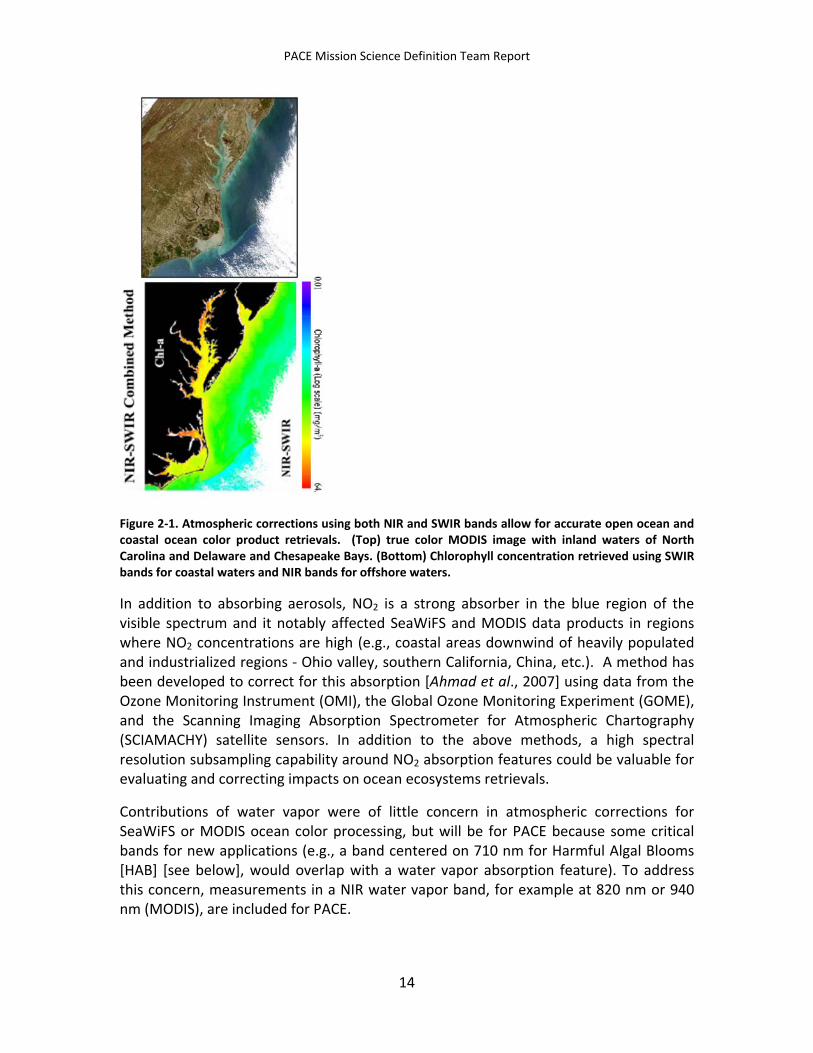
PACE Mission Science Definition Team Report
Figure 2-1. Atmospheric corrections using both NIR and SWIR bands allow for accurate open ocean and coastal ocean color product retrievals. (Top) true color MODIS image with inland waters of North Carolina and Delaware and Chesapeake Bays. (Bottom) Chlorophyll concentration retrieved using SWIR bands for coastal waters and NIR bands for offshore waters.
In addition to absorbing aerosols, NO2 is a strong absorber in the blue region of the visible spectrum and it notably affected SeaWiFS and MODIS data products in regions where NO2 concentrations are high (e.g., coastal areas downwind of heavily populated and industrialized regions - Ohio valley, southern California, China, etc.). A method has been developed to correct for this absorption [Ahmad et al., 2007] using data from the Ozone Monitoring Instrument (OMI), the Global Ozone Monitoring Experiment (GOME), and the Scanning Imaging Absorption Spectrometer for Atmospheric Chartography (SCIAMACHY) satellite sensors. In addition to the above methods, a high spectral resolution subsampling capability around NO2 absorption features could be valuable for evaluating and correcting impacts on ocean ecosystems retrievals.
Contributions of water vapor were of little concern in atmospheric corrections for SeaWiFS or MODIS ocean color processing, but will be for PACE because some critical bands for new applications (e.g., a band centered on 710 nm for Harmful Algal Blooms [HAB] [see below], would overlap with a water vapor absorption feature). To address this concern, measurements in a NIR water vapor band, for example at 820 nm or 940 nm (MODIS), are included for PACE.
14
PACE Mission Science Definition Team Report
PACE’s attention to the atmospheric correction problem will help ensure superior ocean ecosystem properties. Further improvements in atmospheric corrections could be realized with spectral measurements in the oxygen A-band for aerosol heights and bi-directional and polarized measurements for aerosol species.
Summary: PACE includes measurement bands in the UV, NIR, and SWIR for improved atmospheric corrections over open ocean and coastal waters. High resolution measurements in the blue band will also help with assessments of NO2.
2.2.2.2 Separating Dominant Absorbing Components In-water absorbing and scattering constituents vary independently and must be accurately resolved for any one product to be properly assessed. Of particular concern is chromophoric dissolved organic matter (CDOM), which is ubiquitous in the surface ocean [Siegel et al., 2002, 2005]. CDOM dominates light absorption at blue and shorter wavelengths and it interferes with chlorophyll retrievals because its distribution can be quite distinct from that of pigment absorption. Figure 2-2 illustrates the seriousness of this issue. Here, the difference in chlorophyll estimates for a standard wavelength-ratio algorithm and an inversion-based algorithm are shown in the top panel. This difference is compared in the middle panel to the inversion-based estimate of CDOM absorption. This comparison clearly demonstrates that uncertainty in chlorophyll retrievals is directly linked to CDOM. The difference in global annual production for these two chlorophyll estimates is ~16 GtC/yr; in other words, an uncertainty ~30% in annual ocean production! However, it is important to note that at this time, significant uncertainties in both the wavelength ratio product and inversion products remain because of limitations in the heritage measurement bands. We do not yet know which of the two chlorophyll products compared in the top half of Figure 2-2 is more accurate.
15
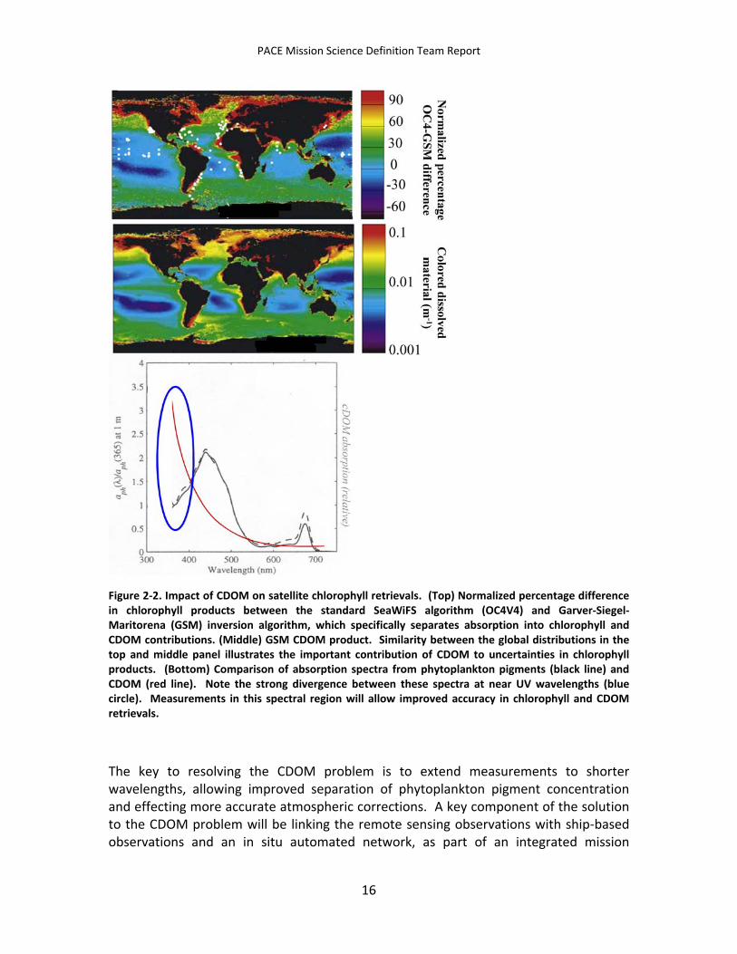
PACE Mission Science Definition Team Report
Figure 2-2. Impact of CDOM on satellite chlorophyll retrievals. (Top) Normalized percentage difference in chlorophyll products between the standard SeaWiFS algorithm (OC4V4) and Garver-Siegel-Maritorena (GSM) inversion algorithm, which specifically separates absorption into chlorophyll and CDOM contributions. (Middle) GSM CDOM product. Similarity between the global distributions in the top and middle panel illustrates the important contribution of CDOM to uncertainties in chlorophyll products. (Bottom) Comparison of absorption spectra from phytoplankton pigments (black line) and CDOM (red line). Note the strong divergence between these spectra at near UV wavelengths (blue circle). Measurements in this spectral region will allow improved accuracy in chlorophyll and CDOM retrievals.
The key to resolving the CDOM problem is to extend measurements to shorter wavelengths, allowing improved separation of phytoplankton pigment concentration and effecting more accurate atmospheric corrections. A key component of the solution to the CDOM problem will be linking the remote sensing observations with ship-based observations and an in situ automated network, as part of an integrated mission
16
PACE Mission Science Definition Team Report
concept. Specifically, phytoplankton pigment absorption generally decreases between 440 nm and 360 nm. In contrast, CDOM absorption continues to increase exponentially well into the UV-A region (Figure 2-2, bottom panel). The CZCS did not have any bands at these shorter wavelengths to effectively separate pigment and CDOM absorption. SeaWiFS, MODIS, and other “second generation” sensors incorporated a band at 412 nm, but even at this wavelength retrieval of CDOM is problematic. PACE will include UV-A bands (e.g., centered at 360 and 380 nm) for quantification of CDOM absorption, and thus improved assessment of phytoplankton pigment concentrations. These improvements will be realized by incorporating the UV bands in advanced inversion algorithms. However, challenges of the inversion approach should be noted. Specifically, while inversions allow the simultaneous retrieval of multiple ocean properties, they are much more sensitive to errors in satellite water-leaving radiances. This issue arises because inversion products are derived by matching composite algorithm spectra with absolute radiances, whereas wavelength ratio algorithms derive products from the relative relationship between particular measurement bands. As a consequence, spectrally independent errors in water-leaving radiances will tend to cancel each other in the wavelength ratio approach, but will directly degrade inversion products in proportion to the error in the satellite radiances. This sensitivity to error in absolute radiance retrievals re-emphasizes the importance of accurate atmospheric corrections.
Summary: PACE includes long-wavelength UV-A bands to effectively separate absorption by CDOM and phytoplankton pigments, yielding far more accurate assessments of productivity.
2.2.2.3 Assessing Phytoplankton Pigment Absorption Chlorophyll-a is a photosynthetic pigment common across all prokaryotic and eukaryotic phytoplankton. It is not, however, the only pigment in these organisms. A wide range of accessory pigments are found among different phytoplankton species. These pigments largely function within the light-harvesting antennae and broaden the spectral range of absorbed light used to drive photosynthetic carbon assimilation (Figure 2-3). The relative ratio of chlorophyll-a absorption to accessory pigment absorption is highly variable in natural plankton populations, and is a function of both taxonomic composition and environmental growth conditions. Pigment diversity amongst phytoplankton gives rise to significant variations in pigment absorption spectra, and accounting for this variability is essential for quantifying ocean productivity because photosynthesis is regulated in proportion to total light absorption, not simply by chlorophyll absorption.
17
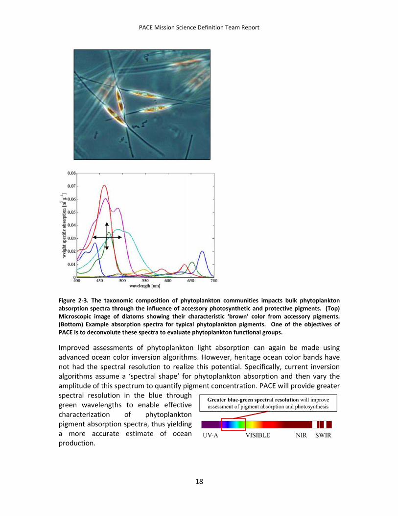
PACE Mission Science Definition Team Report
Figure 2-3. The taxonomic composition of phytoplankton communities impacts bulk phytoplankton absorption spectra through the influence of accessory photosynthetic and protective pigments. (Top) Microscopic image of diatoms showing their characteristic ‘brown’ color from accessory pigments. (Bottom) Example absorption spectra for typical phytoplankton pigments. One of the objectives of PACE is to deconvolute these spectra to evaluate phytoplankton functional groups.
Improved assessments of phytoplankton light absorption can again be made using advanced ocean color inversion algorithms. However, heritage ocean color bands have not had the spectral resolution to realize this potential. Specifically, current inversion algorithms assume a ‘spectral shape’ for phytoplankton absorption and then vary the amplitude of this spectrum to quantify pigment concentration. PACE will provide greater spectral resolution in the blue through green wavelengths to enable effective characterization of phytoplankton pigment absorption spectra, thus yielding a more accurate estimate of ocean production.
18
PACE Mission Science Definition Team Report
Summary: PACE provides high spectral resolution measurements in the visible wavelengths for more accurate assessment of phytoplankton pigment absorption, photosynthesis, and ocean ecology.
2.2.2.4 Ocean Particle Abundances and Living Carbon Stocks Global variations in water-leaving radiance do not reflect changes in the concentration of light absorbing components alone, but also variations in scattering properties. Thus, determination of scattering coefficients is another integral aspect of inversion algorithm solutions. Quite simply, one must accurately characterize variability in scattering to accurately retrieve pigment absorption, and vice versa. In the case of remote sensing analyses, the scattering coefficient resolved is the backscattering coefficient (bb), which is composed of a contribution by water (bbw) and a particulate contribution (bbp). The important property of bbp is that it registers changes in the density of particles and can be related to phytoplankton or total particulate carbon biomass. Analysis of bbp data from SeaWiFS shows that it exhibits significant independent variations from chlorophyll, and thus provides additional critical information about plankton communities. In particular, the bbp–based biomass to chlorophyll ratio provides information on phytoplankton physiology that can be related to growth rates. However, there are complications in deriving phytoplankton carbon from bbp. Most importantly, the particle population contributing to bbp differs in its size dependence from the populations composing total phytoplankton carbon. Thus, to derive the latter from the former, one needs information on the particle size spectrum. In current inversion algorithms, the restricted range and spectral resolution of heritage remote sensing bands strongly constrains the information available on particle scattering, such that in most approaches a single spectral shape for bbp is assumed (Figure 2-4). With additional bands, particularly in the green-to-orange region of the visible spectrum, inversion algorithms can provide information on both the quantity of particles and the particle size distribution, thus yielding more accurate assessments of phytoplankton carbon. PACE will include bands for these improved retrievals.
19
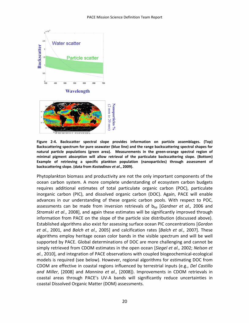
PACE Mission Science Definition Team Report
Figure 2-4. Backscatter spectral slope provides information on particle assemblages. (Top) Backscattering spectrum for pure seawater (blue line) and the range backscattering spectral shapes for natural particle populations (green area). Measurements in the green-orange spectral region of minimal pigment absorption will allow retrieval of the particulate backscattering slope. (Bottom) Example of retrieving a specific plankton population (nanoparticles) through assessment of backscattering slope. (data from Kostadinov et al., 2009).
Phytoplankton biomass and productivity are not the only important components of the ocean carbon system. A more complete understanding of ecosystem carbon budgets requires additional estimates of total particulate organic carbon (POC), particulate inorganic carbon (PIC), and dissolved organic carbon (DOC). Again, PACE will enable advances in our understanding of these organic carbon pools. With respect to POC, assessments can be made from inversion retrievals of bbp [Gardner et al., 2006 and Stramski et al., 2008], and again these estimates will be significantly improved through information from PACE on the slope of the particle size distribution (discussed above). Established algorithms also exist for assessing surface ocean PIC concentrations [Gordon et al., 2001, and Balch et al., 2005] and calcification rates [Balch et al., 2007]. These algorithms employ heritage ocean color bands in the visible spectrum and will be well supported by PACE. Global determinations of DOC are more challenging and cannot be simply retrieved from CDOM estimates in the open ocean [Siegel et al., 2002; Nelson et al., 2010], and integration of PACE observations with coupled biogeochemical-ecological models is required (see below). However, regional algorithms for estimating DOC from CDOM are effective in coastal regions influenced by terrestrial inputs (e.g., Del Castillo and Miller, [2008] and Mannino et al., [2008]). Improvements in CDOM retrievals in coastal areas through PACE’s UV-A bands will significantly reduce uncertainties in coastal Dissolved Organic Matter (DOM) assessments.
20
PACE Mission Science Definition Team Report
Summary: PACE provides high spectral resolution measurements in the visible wavelengths, allowing characterization of particle size distributions and, consequently more accurate assessment of ecosystem carbon stocks
2.2.2.5 Nutrient Stress The relationship between surface phytoplankton pigment concentration and photosynthesis is strongly influenced by variations in the light environment to which phytoplankton are photoacclimated, the degree of nutrient stress (mild to severe), and the type of nutrient stress (e.g., N, P, Fe). These ‘physiological’ factors strongly impact our interpretation/understanding of relationships between climate-forcings and ocean carbon cycling. One nutrient stress of particular significance is iron limitation. Iron availability is tightly coupled to climate through its dependence on aeolian dust deposition, and it is a constraint on productivity over an integrated ocean area that is greater in size than the entire area of Earth covered by land. The role of iron as a major factor limiting global phytoplankton concentrations and primary production [Martin and Fitzwater, 1988] has been studied through a number of iron enrichment experiments and through modeling studies of aeolian dust transport and deposition. Diagnostic indicators of iron stress (i.e., properties that allow iron stress assessment without manipulation of plankton populations) have also been developed, including expression of a photosynthetic electron carrier, flavodoxin, that replaces ferridoxin under low iron conditions [LaRoche et al., 1996], and unique fluorescence properties of the oxygen-evolving photosystem II complex [Behrenfeld et al., 2006]. This latter diagnostic was thoroughly characterized in a basin-wide field fluorescence study [Behrenfeld et al., 2006] and from this work it was predicted that satellite measurements of solar-induced fluorescence could provide a means for assessing global distributions of iron stress. This prediction was verified in a subsequent study [Behrenfeld et al., 2009] where MODIS fluorescence line height (FLH) data were used to calculate global fluorescence quantum yields (φ), after correction for pigment packaging and non-photochemical quenching effects (Figure 2-5). Specifically, the MODIS fluorescence study demonstrated a strong correspondence between elevated φ values, low aeolian dust deposition, and model predictions of iron limited growth [Moore et al., 2006; Moore and Braucher, 2008, Wiggert et al., 2006].
21
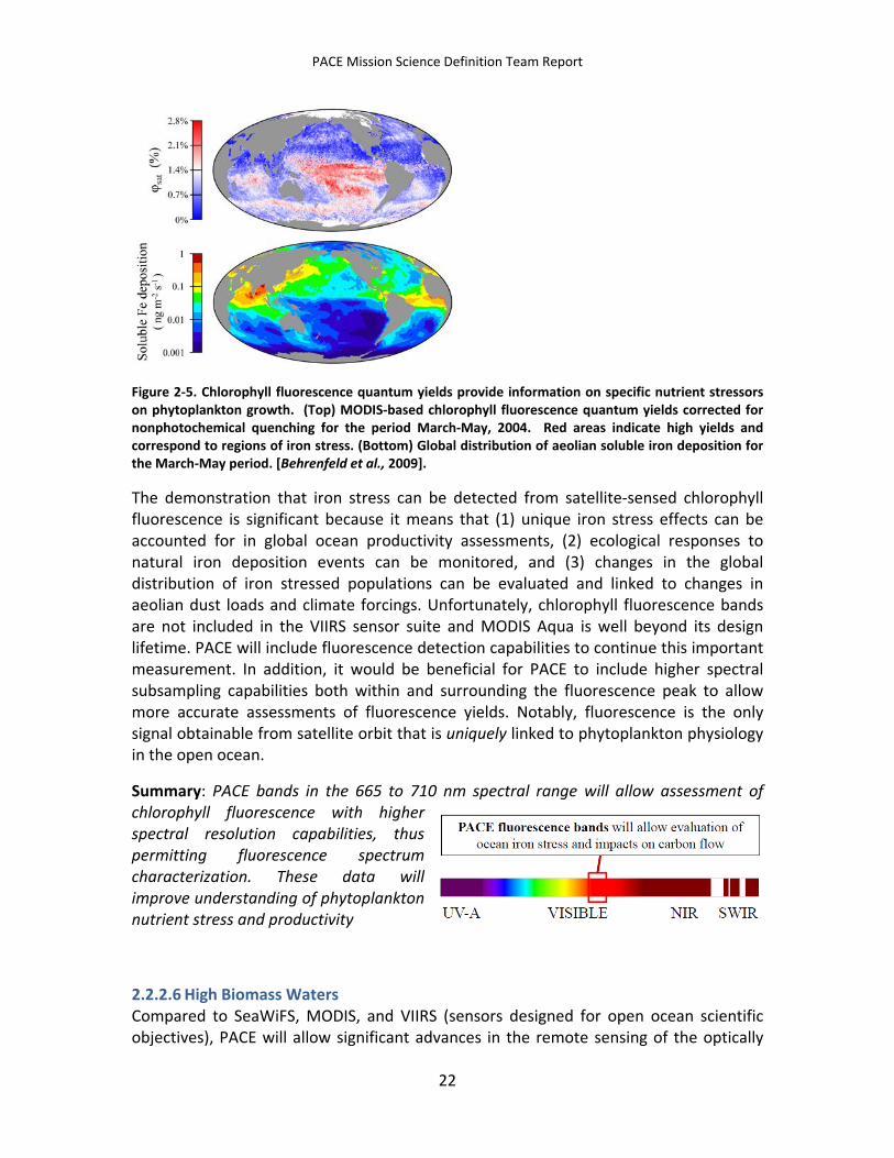
PACE Mission Science Definition Team Report
Figure 2-5. Chlorophyll fluorescence quantum yields provide information on specific nutrient stressors on phytoplankton growth. (Top) MODIS-based chlorophyll fluorescence quantum yields corrected for nonphotochemical quenching for the period March-May, 2004. Red areas indicate high yields and correspond to regions of iron stress. (Bottom) Global distribution of aeolian soluble iron deposition for the March-May period. [Behrenfeld et al., 2009].
The demonstration that iron stress can be detected from satellite-sensed chlorophyll fluorescence is significant because it means that (1) unique iron stress effects can be accounted for in global ocean productivity assessments, (2) ecological responses to natural iron deposition events can be monitored, and (3) changes in the global distribution of iron stressed populations can be evaluated and linked to changes in aeolian dust loads and climate forcings. Unfortunately, chlorophyll fluorescence bands are not included in the VIIRS sensor suite and MODIS Aqua is well beyond its design lifetime. PACE will include fluorescence detection capabilities to continue this important measurement. In addition, it would be beneficial for PACE to include higher spectral subsampling capabilities both within and surrounding the fluorescence peak to allow more accurate assessments of fluorescence yields. Notably, fluorescence is the only signal obtainable from satellite orbit that is uniquely linked to phytoplankton physiology in the open ocean.
Summary: PACE bands in the 665 to 710 nm spectral range will allow assessment of chlorophyll fluorescence with higher spectral resolution capabilities, thus permitting fluorescence spectrum characterization. These data will improve understanding of phytoplankton nutrient stress and productivity
2.2.2.6 High Biomass Waters Compared to SeaWiFS, MODIS, and VIIRS (sensors designed for open ocean scientific objectives), PACE will allow significant advances in the remote sensing of the optically
22
PACE Mission Science Definition Team Report
complex ocean margins and larger estuarine and freshwater systems. These areas form the interface between the terrestrial and open ocean provinces and are sites of very high primary production rates and biogeochemical transformations of carbon, nitrogen, and phosphorous. These processes are particularly important where freshwater discharge from major terrestrial drainage basins and or/population centers are focused (e.g., Mississippi River delta, Chesapeake Bay, San Francisco Bay, Gulf of Maine, Pamlico Sound, and Puget Sound). Accordingly, PACE data will be valuable for supporting coastal management and environmental monitoring, as well as basic science applications.
In addition to the smaller spatial scales of variability in inland and near-shore waters, a major remote sensing challenge in regions with high suspended particle loads, dissolved organic matter concentrations, and terrestrial inputs is the separation of these optically active components from each other and from the resident plankton populations. This separation will be enabled through PACE in a manner unparalleled by heritage sensors, through its high spectral resolution in the UV-A to green wavebands. In addition, some of these areas experience significant eutrophication. In waters with high concentrations of absorbing constituents, water-leaving radiances in the UV and blue are very small, rendering them of marginal use for deriving geophysical products (due to loss of sensitivity). However, algorithms have emerged for such aquatic applications that utilize the fluorescence properties of phytoplankton in the red to separate them from CDOM-rich river plumes, and long wavelengths in the red and short NIR bands to extract phytoplankton levels in a manner similar to terrestrial leaf area cover algorithms (Figure 2-6). PACE’s full resolution in the ‘red-edge’ spectral region will allow application of these algorithms.
23
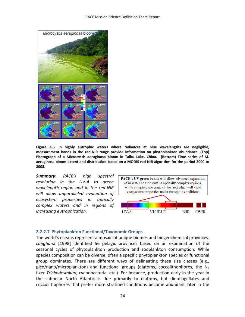
PACE Mission Science Definition Team Report
Figure 2-6. In highly eutrophic waters where radiances at blue wavelengths are negligible, measurement bands in the red-NIR range provide information on phytoplankton abundance. (Top) Photograph of a Microcystis aeruginosa bloom in Taihu Lake, China. (Bottom) Time series of M. aeruginosa bloom extent and distribution based on a MODIS red-NIR algorithm for the period 2000 to 2008.
Summary: PACE’s high spectral resolution in the UV-A to green wavelength region and in the red-NIR will allow unparalleled evaluation of ecosystem properties in optically complex waters and in regions of increasing eutrophication.
2.2.2.7 Phytoplankton Functional/Taxonomic Groups The world’s oceans represent a mosaic of unique biomes and biogeochemical provinces. Longhurst [1998] identified 56 pelagic provinces based on an examination of the seasonal cycles of phytoplankton production and zooplankton consumption. While species composition can be diverse, often a specific phytoplankton species or functional group dominates. There are different ways of delineating these size classes (e.g., pico/nano/microplankton) and functional groups (diatoms, coccolithophores, the N2 fixer Trichodesmium, cyanobacteria, etc.). For instance, production early in the year in the subpolar North Atlantic is due primarily to diatoms, but dinoflagellates and coccolithophores that prefer more stratified conditions become abundant later in the
24
PACE Mission Science Definition Team Report
summer. Thus, phytoplankton populations vary in their biomass, species composition, photosynthetic efficiency, etc., depending on the physical environment, availability of macro- and micro-nutrients, illumination, and concentration of grazers. These variations regulate primary production and, therefore, higher trophic levels within the ecosystem, and play an important role in the cycling of macro- and micro-nutrient concentrations. Identifying these distributions and properties and determining how they change on seasonal and interannual time scales is key to understanding how ecosystems function and how they respond to changes in the physical environment, whether natural or human-induced.
Until recently, research on optical identification of specific species has focused on coccolithophores and Trichodesmium because of their rather unique spectral reflectance signatures. Coccolithophores have calcite platelets that can be identified in satellite data because, at high concentrations, their reflectance is uniformly elevated across the spectrum. Global coccolithophore distributions were first assessed using CZCS data [Brown and Yoder, 1994] and will be easily detectable with the PACE measurement spectrum.
Another phytoplankton genus with a distinctive spectral signature is the nitrogen-fixing cyanobacterium, Trichodesmium. This biogeochemically important species has gas-filled vacuoles or trichomes, elevated specific absorption coefficients below 443 nm, and enhanced particle backscatter coefficients at visible wavelengths. Westberry et al. [2005] found that if the concentration of trichomes is sufficiently high (3200/l), detection by SeaWiFS is possible. Westberry and Siegel [2006] mapped Trichodesmium globally using SeaWiFS data and found their derived distribution to be consistent with geochemical inferences made by Deutsch et al. [2007]. More recently, Hu et al. [2010] combined MODIS land and ocean bands in the visible and NIR to establish a higher spectral resolution algorithm closely reproducing Trichodesmium absorption measured in the field. All of these approaches for assessing Trichodesmium populations will be supported by the improved spectral resolution of PACE, as well as the development of new algorithms.
Coccolithophores and Trichodesmium have relatively unique signatures in water-leaving radiance spectra. However, characterization of other dominant phytoplankton groups has also been demonstrated through detection of subtle differences in reflectance spectra associated with specific diagnostic pigments. For example, Alvain et al. [2005] used in situ databases of reflectance, pigments, functional groups and SeaWiFS reflectances to estimate global open ocean distributions of haptophytes, Prochlorococcus, Synechococcus-like cyanobacteria (SLC), and diatoms. However, given the limited number of spectral bands that heritage sensors have, this separation is challenging and resultant group distributions have large uncertainties and are difficult to verify.
Enhancing the spectral resolution and spectral range of ocean color measurements can greatly enhance retrieved information on plankton composition. The approach for using
25
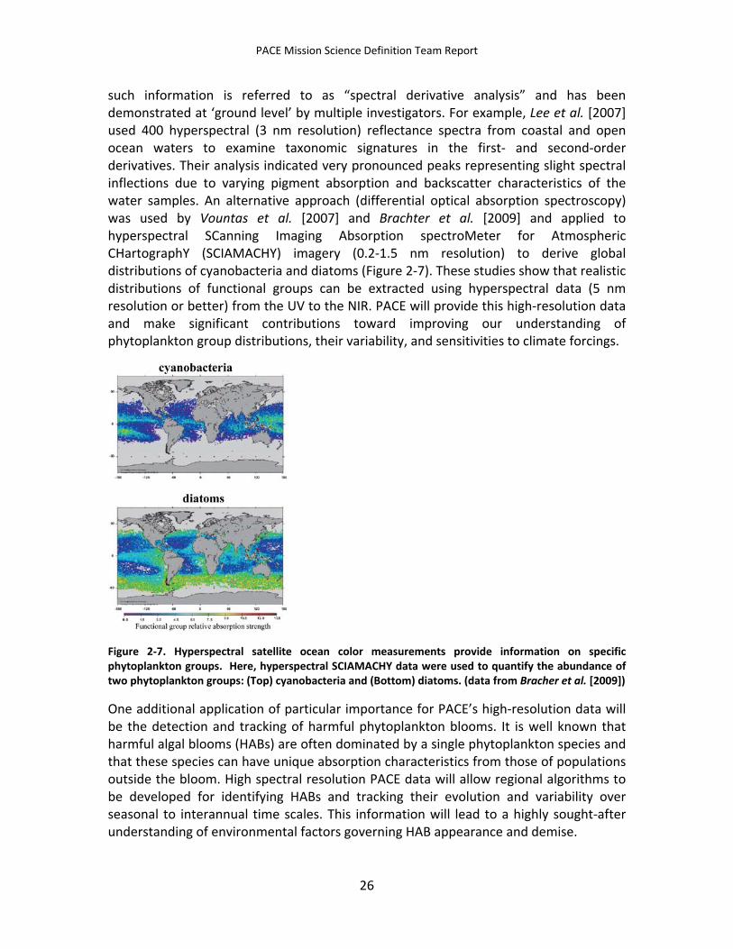
PACE Mission Science Definition Team Report
such information is referred to as “spectral derivative analysis” and has been demonstrated at ‘ground level’ by multiple investigators. For example, Lee et al. [2007] used 400 hyperspectral (3 nm resolution) reflectance spectra from coastal and open ocean waters to examine taxonomic signatures in the first- and second-order derivatives. Their analysis indicated very pronounced peaks representing slight spectral inflections due to varying pigment absorption and backscatter characteristics of the water samples. An alternative approach (differential optical absorption spectroscopy) was used by Vountas et al. [2007] and Brachter et al. [2009] and applied to hyperspectral SCanning Imaging Absorption spectroMeter for Atmospheric CHartographY (SCIAMACHY) imagery (0.2-1.5 nm resolution) to derive global distributions of cyanobacteria and diatoms (Figure 2-7). These studies show that realistic distributions of functional groups can be extracted using hyperspectral data (5 nm resolution or better) from the UV to the NIR. PACE will provide this high-resolution data and make significant contributions toward improving our understanding of phytoplankton group distributions, their variability, and sensitivities to climate forcings.
Figure 2-7. Hyperspectral satellite ocean color measurements provide information on specific phytoplankton groups. Here, hyperspectral SCIAMACHY data were used to quantify the abundance of two phytoplankton groups: (Top) cyanobacteria and (Bottom) diatoms. (data from Bracher et al. [2009])
One additional application of particular importance for PACE’s high-resolution data will be the detection and tracking of harmful phytoplankton blooms. It is well known that harmful algal blooms (HABs) are often dominated by a single phytoplankton species and that these species can have unique absorption characteristics from those of populations outside the bloom. High spectral resolution PACE data will allow regional algorithms to be developed for identifying HABs and tracking their evolution and variability over seasonal to interannual time scales. This information will lead to a highly sought-after understanding of environmental factors governing HAB appearance and demise.
26
PACE Mission Science Definition Team Report
Summary: PACE UV-A and visible hyperspectral data allow discrimination of functional/taxonomic/harmful algal groups to improve understanding of their dynamics, sensitivity to climate forcings, and impacts on ocean carbon cycles
2.2.2.8 Photosynthesis and Phytoplankton Productivity Only at the turn of the 19th century did scientists recognize that most major fisheries and other marine ecosystem components were sustained by the microscopic free-floating plants called phytoplankton, rather than by subsidies from terrestrial ecosystems. Net primary production (NPP) by phytoplankton (NPP; roughly 60 Pg C y-1) represents at least half of the net plant production of the biosphere and is the major conduit for biologically sequestering atmospheric carbon dioxide into moderate- and long-lifetime organic ocean carbon pools. In addition to being a key climate-controlling process, its quantification allows investigations into energy transfer throughout marine food webs and is a critical attribute in near-shore waters with respect to the potential for harmful algal blooms and changes in water quality. Phytoplankton productivity is a key metric of ocean ecosystem health, stability, and structure.
Two terms are needed to quantify net primary production: the standing stock of phytoplankton biomass and the biomass-specific productivity rate. For 50 years, chlorophyll concentration has functioned as the central metric of phytoplankton biomass. Indeed, NASA’s previous ocean color missions (CZCS, SeaWiFS, MODIS) have focused on surface chlorophyll biomass as the primary biologically relevant remote sensing product. Using chlorophyll concentration as a single proxy of photosynthesis, however, has a critical flaw that will forever prevent ocean photosynthesis from being accurately quantified: namely, chlorophyll is not simply a function of biomass, but instead a complex function of biomass and growth conditions. The rate term needed to convert chlorophyll biomass into primary production (i.e., chlorophyll-specific photosynthetic efficiency) behaves in a very complicated manner, and its description requires information on growth constraints that are difficult to measure in the field and impossible to derive from space. In addition, assessing changes in phytoplankton biomass and physiology relies on an accurate separation of absorption by the diverse suspended components in the upper ocean. So, how important is it to distinguish physiological variability from biomass and pigment changes from other absorbing compounds? A good example is provided by our current ocean color data record.
Figure 2-8 shows the observed chlorophyll changes from SeaWiFS and MODIS for the period 1997 to 2008. The data are separated into broad regions of the high northern latitudes (top panel), the central permanently stratified oceans (middle panel), and the high latitude southern oceans (bottom panel). For this figure, the seasonal cycle in
27
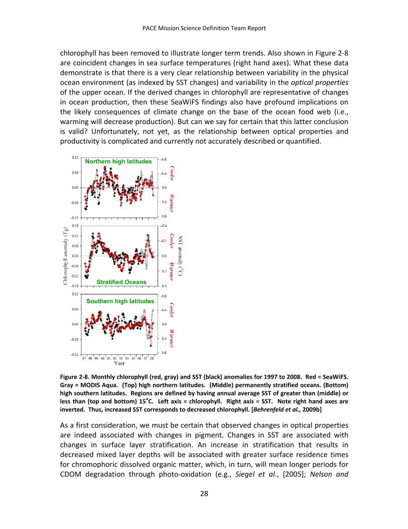
PACE Mission Science Definition Team Report
chlorophyll has been removed to illustrate longer term trends. Also shown in Figure 2-8 are coincident changes in sea surface temperatures (right hand axes). What these data demonstrate is that there is a very clear relationship between variability in the physical ocean environment (as indexed by SST changes) and variability in the optical properties of the upper ocean. If the derived changes in chlorophyll are representative of changes in ocean production, then these SeaWiFS findings also have profound implications on the likely consequences of climate change on the base of the ocean food web (i.e., warming will decrease production). But can we say for certain that this latter conclusion is valid? Unfortunately, not yet, as the relationship between optical properties and productivity is complicated and currently not accurately described or quantified.
Figure 2-8. Monthly chlorophyll (red, gray) and SST (black) anomalies for 1997 to 2008. Red = SeaWiFS. Gray = MODIS Aqua. (Top) high northern latitudes. (Middle) permanently stratified oceans. (Bottom) high southern latitudes. Regions are defined by having annual average SST of greater than (middle) or less than (top and bottom) 15oC. Left axis = chlorophyll. Right axis = SST. Note right hand axes are inverted. Thus, increased SST corresponds to decreased chlorophyll. [Behrenfeld et al., 2009b]
As a first consideration, we must be certain that observed changes in optical properties are indeed associated with changes in pigment. Changes in SST are associated with changes in surface layer stratification. An increase in stratification that results in decreased mixed layer depths will be associated with greater surface residence times for chromophoric dissolved organic matter, which, in turn, will mean longer periods for CDOM degradation through photo-oxidation (e.g., Siegel et al., [2005]; Nelson and
28
PACE Mission Science Definition Team Report
Siegel, in review). Thus, accurately distinguishing CDOM changes from pigment changes is essential. This is an important reason for extension of PACE measurements into UV-A bands.
A second issue is that if the changes shown in Figure 2-8 truly represent changes in chlorophyll, then the co-variation in chlorophyll and stratification (i.e., SST) could be due primarily to phytoplankton physiological responses to changes in average mixed layer light levels. In other words, increased surface stratification increases mixed layer light levels and causes phytoplankton to decrease intracellular chlorophyll without a requisite decrease in NPP.
A third issue is that lack of nutrient supply will lead to lack of growth and production, increased recycling and various losses. Phytoplankton also simply accumulates at a deeper depth, which may be inaccessible to satellite observations—this is another reason why the PACE mission requires an integrated space-based and ground-based approach to answering basic science questions. Thus, it is absolutely essential to distinguish physiological changes from phytoplankton biomass changes to accurately understand observed relationships between climate variability and ocean ecosystems. Accordingly, PACE has an expanded band set to quantify phytoplankton carbon stocks from backscattering properties, as well as to improve assessments of phytoplankton pigment absorption. Finally, the relationship between environmental variability and phytoplankton biomass and physiological characteristics is strongly dependent on the type of nutrient limiting growth (e.g., iron) and the taxonomic composition of the phytoplankton community. Thus, PACE has advanced chlorophyll fluorescence detection capabilities and hyperspectral resolution to evaluate nutrient stress and taxonomic groups.
Summary: The expanded set of phytoplankton-related properties retrieved by PACE will allow more accurate characterization and separation of phytoplankton biomass and physiological variability from other optical properties, leading to improved descriptions of carbon assimilation efficiencies and thus quantification of NPP.
2.2.2.9 Net Community Production and Carbon Export Upper ocean carbon stocks are comprised of both organic (POC and DOC) and inorganic (Dissolved inorganic carbon [DIC] and PIC) forms of carbon. A key issue in understanding ocean biogeochemical carbon fluxes is resolving interactions between these forms. Phytoplankton productivity (discussed above) is the major mechanism converting dissolved inorganic carbon into particulate form in the upper ocean. However, a myriad of food web processes cycle organic carbon fixed by phytoplankton into other forms—both organic and inorganic (Figure 2-9). These food web processes include (but are not limited to) the heterotrophic respiration of organic carbon to DIC, export of POC from the upper ocean by sinking particles, export of DOC by convective mixing, and export by vertically migrating zooplankton. The net balance between phytoplankton production
29
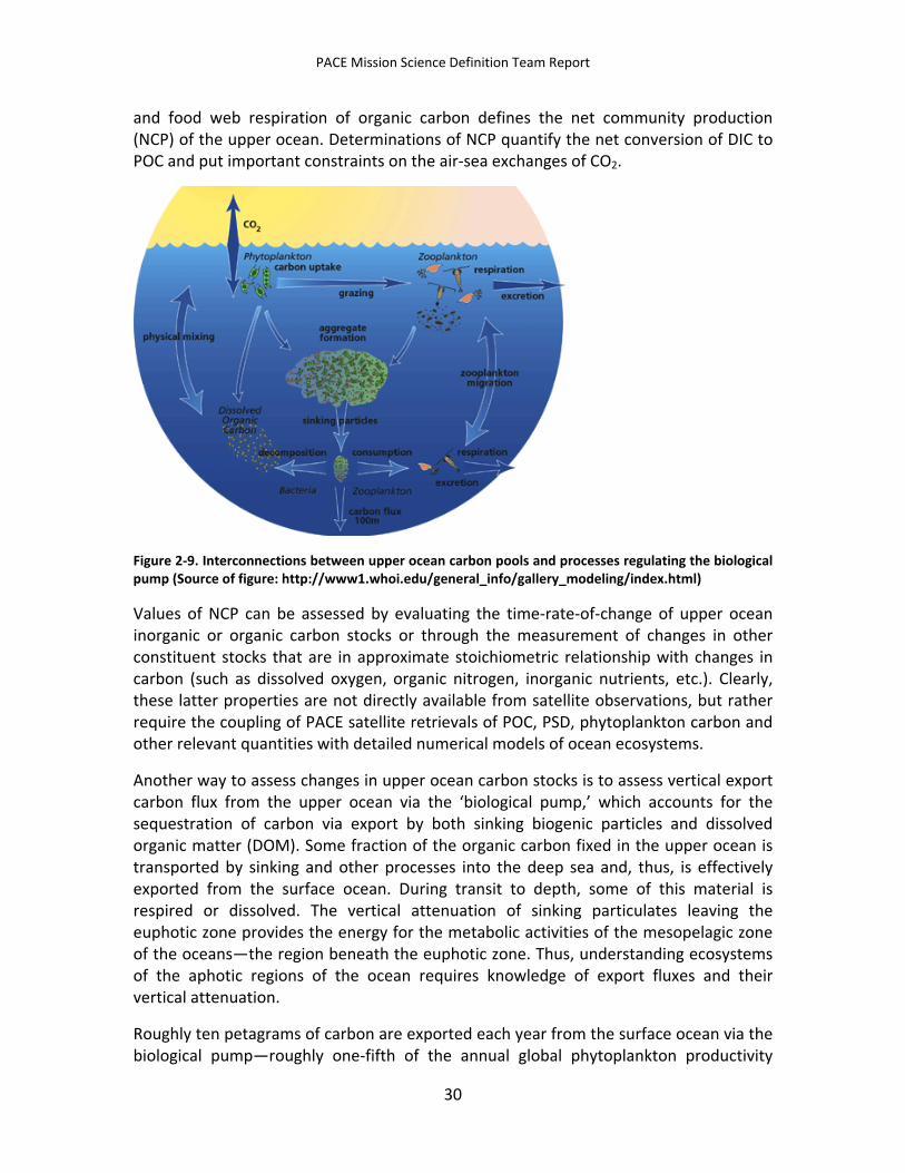
PACE Mission Science Definition Team Report
and food web respiration of organic carbon defines the net community production (NCP) of the upper ocean. Determinations of NCP quantify the net conversion of DIC to POC and put important constraints on the air-sea exchanges of CO2.
Figure 2-9. Interconnections between upper ocean carbon pools and processes regulating the biological pump (Source of figure: http://www1.whoi.edu/general_info/gallery_modeling/index.html)
Values of NCP can be assessed by evaluating the time-rate-of-change of upper ocean inorganic or organic carbon stocks or through the measurement of changes in other constituent stocks that are in approximate stoichiometric relationship with changes in carbon (such as dissolved oxygen, organic nitrogen, inorganic nutrients, etc.). Clearly, these latter properties are not directly available from satellite observations, but rather require the coupling of PACE satellite retrievals of POC, PSD, phytoplankton carbon and other relevant quantities with detailed numerical models of ocean ecosystems.
Another way to assess changes in upper ocean carbon stocks is to assess vertical export carbon flux from the upper ocean via the ‘biological pump,’ which accounts for the sequestration of carbon via export by both sinking biogenic particles and dissolved organic matter (DOM). Some fraction of the organic carbon fixed in the upper ocean is transported by sinking and other processes into the deep sea and, thus, is effectively exported from the surface ocean. During transit to depth, some of this material is respired or dissolved. The vertical attenuation of sinking particulates leaving the euphotic zone provides the energy for the metabolic activities of the mesopelagic zone of the oceans—the region beneath the euphotic zone. Thus, understanding ecosystems of the aphotic regions of the ocean requires knowledge of export fluxes and their vertical attenuation.
Roughly ten petagrams of carbon are exported each year from the surface ocean via the biological pump—roughly one-fifth of the annual global phytoplankton productivity
30
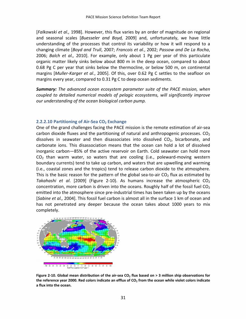
PACE Mission Science Definition Team Report
[Falkowski et al., 1998]. However, this flux varies by an order of magnitude on regional and seasonal scales [Buesseler and Boyd, 2009] and, unfortunately, we have little understanding of the processes that control its variability or how it will respond to a changing climate [Boyd and Trull, 2007; Francois et al., 2002; Passow and De La Rocha, 2006; Balch et al., 2010]. For example, only about 1 Pg per year of this particulate organic matter likely sinks below about 800 m in the deep ocean, compared to about 0.68 Pg C per year that sinks below the thermocline, or below 500 m, on continental margins [Muller-Karger et al., 2005]. Of this, over 0.62 Pg C settles to the seafloor on margins every year, compared to 0.31 Pg C to deep ocean sediments.
Summary: The advanced ocean ecosystem parameter suite of the PACE mission, when coupled to detailed numerical models of pelagic ecosystems, will significantly improve our understanding of the ocean biological carbon pump.
2.2.2.10 Partitioning of Air-Sea CO2 Exchange One of the grand challenges facing the PACE mission is the remote estimation of air-sea carbon dioxide fluxes and the partitioning of natural and anthropogenic processes. CO2 dissolves in seawater and then disassociates into dissolved CO2, bicarbonate, and carbonate ions. This disassociation means that the ocean can hold a lot of dissolved inorganic carbon—85% of the active reservoir on Earth. Cold seawater can hold more CO2 than warm water, so waters that are cooling (i.e., poleward-moving western boundary currents) tend to take up carbon, and waters that are upwelling and warming (i.e., coastal zones and the tropics) tend to release carbon dioxide to the atmosphere. This is the basic reason for the pattern of the global sea-to-air CO2 flux as estimated by Takahashi et al. [2009] (Figure 2-10). As humans increase the atmospheric CO2 concentration, more carbon is driven into the oceans. Roughly half of the fossil fuel CO2 emitted into the atmosphere since pre-industrial times has been taken up by the oceans [Sabine et al., 2004]. This fossil fuel carbon is almost all in the surface 1 km of ocean and has not penetrated any deeper because the ocean takes about 1000 years to mix completely.
Figure 2-10. Global mean distribution of the air-sea CO2 flux based on > 3 million ship observations for the reference year 2000. Red colors indicate an efflux of CO2 from the ocean while violet colors indicate a flux into the ocean.
31
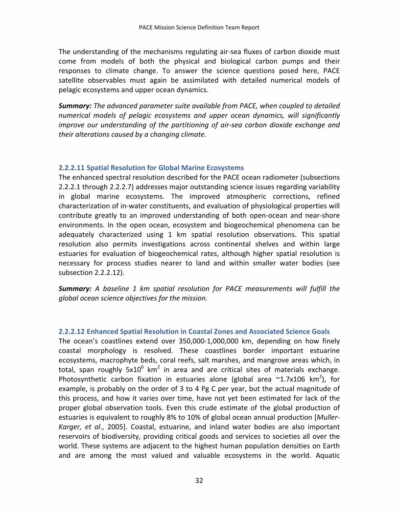
PACE Mission Science Definition Team Report
The understanding of the mechanisms regulating air-sea fluxes of carbon dioxide must come from models of both the physical and biological carbon pumps and their responses to climate change. To answer the science questions posed here, PACE satellite observables must again be assimilated with detailed numerical models of pelagic ecosystems and upper ocean dynamics.
Summary: The advanced parameter suite available from PACE, when coupled to detailed numerical models of pelagic ecosystems and upper ocean dynamics, will significantly improve our understanding of the partitioning of air-sea carbon dioxide exchange and their alterations caused by a changing climate.
2.2.2.11 Spatial Resolution for Global Marine Ecosystems The enhanced spectral resolution described for the PACE ocean radiometer (subsections 2.2.2.1 through 2.2.2.7) addresses major outstanding science issues regarding variability in global marine ecosystems. The improved atmospheric corrections, refined characterization of in-water constituents, and evaluation of physiological properties will contribute greatly to an improved understanding of both open-ocean and near-shore environments. In the open ocean, ecosystem and biogeochemical phenomena can be adequately characterized using 1 km spatial resolution observations. This spatial resolution also permits investigations across continental shelves and within large estuaries for evaluation of biogeochemical rates, although higher spatial resolution is necessary for process studies nearer to land and within smaller water bodies (see subsection 2.2.2.12).
Summary: A baseline 1 km spatial resolution for PACE measurements will fulfill the global ocean science objectives for the mission.
2.2.2.12 Enhanced Spatial Resolution in Coastal Zones and Associated Science Goals The ocean’s coastlines extend over 350,000-1,000,000 km, depending on how finely coastal morphology is resolved. These coastlines border important estuarine ecosystems, macrophyte beds, coral reefs, salt marshes, and mangrove areas which, in total, span roughly 5x10⁶ km2 in area and are critical sites of materials exchange. Photosynthetic carbon fixation in estuaries alone (global area ~1.7x10⁶ km2), for example, is probably on the order of 3 to 4 Pg C per year, but the actual magnitude of this process, and how it varies over time, have not yet been estimated for lack of the proper global observation tools. Even this crude estimate of the global production of estuaries is equivalent to roughly 8% to 10% of global ocean annual production [Muller-Karger, et al., 2005]. Coastal, estuarine, and inland water bodies are also important reservoirs of biodiversity, providing critical goods and services to societies all over the world. These systems are adjacent to the highest human population densities on Earth and are among the most valued and valuable ecosystems in the world. Aquatic
32
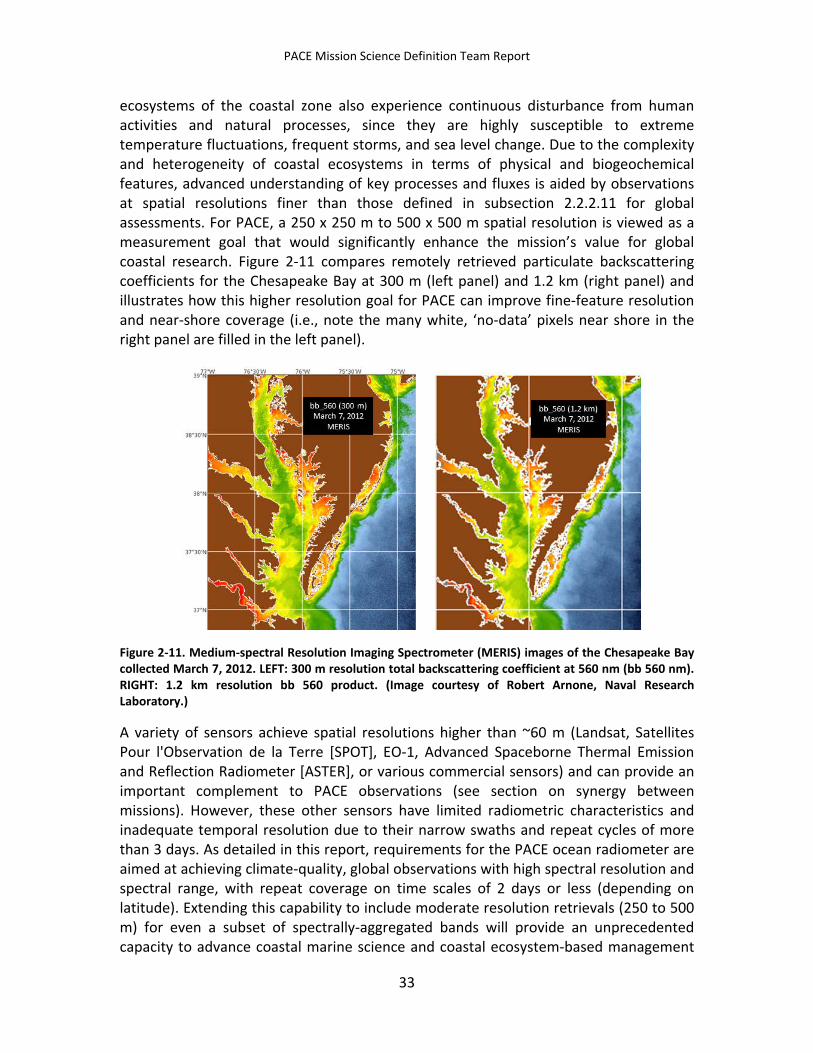
PACE Mission Science Definition Team Report
ecosystems of the coastal zone also experience continuous disturbance from human activities and natural processes, since they are highly susceptible to extreme temperature fluctuations, frequent storms, and sea level change. Due to the complexity and heterogeneity of coastal ecosystems in terms of physical and biogeochemical features, advanced understanding of key processes and fluxes is aided by observations at spatial resolutions finer than those defined in subsection 2.2.2.11 for global assessments. For PACE, a 250 x 250 m to 500 x 500 m spatial resolution is viewed as a measurement goal that would significantly enhance the mission’s value for global coastal research. Figure 2-11 compares remotely retrieved particulate backscattering coefficients for the Chesapeake Bay at 300 m (left panel) and 1.2 km (right panel) and illustrates how this higher resolution goal for PACE can improve fine-feature resolution and near-shore coverage (i.e., note the many white, ‘no-data’ pixels near shore in the right panel are filled in the left panel).
Figure 2-11. Medium-spectral Resolution Imaging Spectrometer (MERIS) images of the Chesapeake Bay collected March 7, 2012. LEFT: 300 m resolution total backscattering coefficient at 560 nm (bb 560 nm). RIGHT: 1.2 km resolution bb 560 product. (Image courtesy of Robert Arnone, Naval Research Laboratory.)
A variety of sensors achieve spatial resolutions higher than ~60 m (Landsat, Satellites Pour l'Observation de la Terre [SPOT], EO-1, Advanced Spaceborne Thermal Emission and Reflection Radiometer [ASTER], or various commercial sensors) and can provide an important complement to PACE observations (see section on synergy between missions). However, these other sensors have limited radiometric characteristics and inadequate temporal resolution due to their narrow swaths and repeat cycles of more than 3 days. As detailed in this report, requirements for the PACE ocean radiometer are aimed at achieving climate-quality, global observations with high spectral resolution and spectral range, with repeat coverage on time scales of 2 days or less (depending on latitude). Extending this capability to include moderate resolution retrievals (250 to 500 m) for even a subset of spectrally-aggregated bands will provide an unprecedented capacity to advance coastal marine science and coastal ecosystem-based management
33
PACE Mission Science Definition Team Report
applications. The global coverage requirement for PACE also ensures that the higher spatial resolution retrievals will yield an unprecedented temporal resolution for investigating variability in coastal zone processes and features. Higher spatial resolution retrievals will address four goal Coastal Science Questions (CSQ) that are consistent with the overarching PACE threshold ocean science questions:
CSQ-1: What is the distribution of habitat and ecosystems and the variability of biogeochemical parameters at moderate scales (250-500 m) and what is the impact on coastal (estuarine, tidal wetlands, lakes) biodiversity and other coastal ecosystem services?
CSQ-2: What is the connectivity between coastal, shelf, and offshore environments?
CSQ-3: How does the export of terrestrial material affect the composition of phytoplankton functional types in coastal waters, and how do these in turn affect the cycling of organic matter?
CSQ-4: How do moderate scale processes (sedimentation, photodegradation, respiration) affect the cycling of terrigenous organic material in the coastal environment?
Moderate-resolution retrievals will increase the area of coastal and inland waters observed by PACE, including the Great Lakes and a large number of smaller water bodies. The capability to image closer to land than allowed with 1 km2 spatial resolution imagery can (1) improve estimates of terrestrial carbon, nutrient, and sediment export, (2) enhance understanding of transformation pathways for carbon and other elements (physical, photochemical, biogeochemical) at the land-ocean interface, (3) inform and improve estuarine and coastal biogeochemical models, and (4) help reduce current uncertainties in the coastal carbon budgets. For example, higher spatial resolution data can reduce uncertainties in carbon export from large rivers by capturing near-shore fluxes and processes nearer than 1 km for shore, and can improve our understanding of linkages between harmful algal blooms and riverine discharges. Regarding this latter issue, legacy ocean color data at 1 km resolution has led to the belief that many HAB blooms are of oceanic or shelf origin, yet recent Medium-spectral Resolution Imaging Spectrometer (MERIS) data at 300 m resolution clearly show that some of these blooms in Florida are linked to smaller rivers. For carbon flux studies, high resolution data will help determine more directly how particulate and dissolved materials change along the course of rivers, how much material enters the coastal zone, and what key transformations take place during transport.
Additional benefits of moderate spatial resolution PACE retrievals may include (1) improved temporal resolution under broken cloud conditions, (2) improved satellite-field product matchup statistics in spatially heterogeneous waters due to improved correspondence of measurement scales, and (3) increased use of ocean color in coastal research and management applications around the globe. This latter benefit is relevant to water quality monitoring; water resource management; eutrophication and oil spill
34
PACE Mission Science Definition Team Report
monitoring; detection, forecasting and early warnings of HABs; and protecting and improving human health (e.g., improved models of abundances of fecal coliforms, Vibrio sp. and nuisance species like sea nettles and harmful algal blooms). Higher resolution data will permit improved products to assess environmental parameters that affect seagrasses and coral reefs, and development of new frequent and synoptic products with national security importance, such as underwater visibility and bathymetry.
In this subsection, we have described the relevance of higher spatial resolution ocean observations for coastal zones, identified four goal coastal science questions addressed with such data, and highlighted just a subset of the science and applications benefits. However, as with all other PACE mission goals described in this report, achieving higher spatial resolution data must not compromise any of the threshold ocean requirements defined for the mission at the baseline resolution of 1 km2 that are delineated in subsections 3.2.1 to 3.2.9. Furthermore, many of the high spatial resolution objectives outlined in this subsection for coastal waters require quantitative (not simply qualitative) property retrievals. Consequently, measurement requirements to achieve these goals are no less stringent than those identified for the 1 km2 global products, and in some cases are more stringent. For example, many of the coastal waters referred to in this subsection are characterized by turbid conditions where typical water-leaving reflectances are substantially lower than typical open ocean values, particularly at the shorter visible and near-ultraviolet (NUV) wavelengths. This characteristic implies that required SNRs at these wavelengths must be greater than for open ocean conditions to achieve acceptable product uncertainties. This issue is discussed in more detail in section 3.2.9, but it places significant constraints on instrument requirements and achievable spectral resolutions at moderate spatial resolution. Clearly, this measurement goal for PACE is an area where engineering innovation is required to achieve better than 1 km2 resolution while maintaining all the sensor attributes specified for the 1 km2 resolution data set.
Summary: A moderate spatial resolution of 250 x 250 m to 500 x 500 m is a measurement goal for PACE that would contribute to an improved understanding of ecosystem and biogeochemical processes in near-shore waters and increase the value of the mission to coastal science and management/monitoring applications.
2.2.2.13 PACE Ocean Science Implementation In the opening statements of this Ocean Ecosystems and Biogeochemistry section, we emphasize the importance of viewing PACE from a ‘whole mission’ perspective. What this means is that achieving the objectives of any NASA ocean mission requires careful attention to the many additional requirements for success beyond assuring superior satellite measurements. In the case of PACE, this statement is particularly true, as our focused science questions entail new product retrievals and assessments of properties that have evaded earlier missions.
35
PACE Mission Science Definition Team Report
As has been abundantly clear from heritage mission experiences, an essential component of the PACE mission will be the establishment and maintenance of a rigorous field-based calibration program. This calibration effort must be closely aligned, and preferably co-located, with the mission flight program office. Planning for the calibration component of PACE and evaluation of measurement systems should begin immediately, with a target for field deployment of one year before launch at the latest. Because of the importance of this mission element to achieving climate quality data, a detailed description of the necessary calibration program has been included in this report in section 4.6.1.
In addition to vicarious sensor calibration, success in the PACE mission science objectives requires a field-based product validation program. Again, organization of this effort should begin immediately and continue through the lifetime of the mission. The overall objective of the validation program is to ensure the highest quality PACE ocean products. Achieving this objective requires focused science teams, development of measurement protocols and algorithms, round-robin testing exercises, intensive and extensive field measurement campaigns, process studies, and evaluations of product uncertainties. It is recommended that these activities be organized under a central coordinating office, also closely aligned with the flight program office. A key attribute of the validation program will be the assemblage of field data sets that capture the broad dynamic ranges and temporal evolution of ecosystem and biogeochemical properties. As described in detail in section 4.6.1, these data sets are indispensable for success of the PACE mission. Accordingly, a validation program needs to be included in the funding profile for the PACE mission, including dedicated ship deployments at the minimum frequency of two cruises per year. Complete reliance on open berths on cruises of opportunity is an inadequate and high-risk approach to product validation, although such opportunities will provide an important data augmentation to the core PACE field program (see additional details in section 4.6.1).
Finally, the vicarious validation and calibration programs should be viewed in the same interdisciplinary manner as the PACE mission as a whole. As described at length in this document, PACE science integrates aquatic, atmospheric, and terrestrial disciplines. The specific science objectives within and between these disciplines all rely on detailed sensor characterization and calibration and on field measurements for product validation.
2.2.2.14 Heritage and Concurrent Sensors The eleven preceding subsections describe specific ocean science issues that will be addressed through the advanced capabilities of PACE. However, another critical objective of PACE is its contribution to the historical ocean biology climate data record. This continuous record began with the SeaWiFS and has been maintained through MODIS, MERIS, and now VIIRS. The expanded objectives of PACE require even greater attention to atmospheric corrections, instrument calibration/validation, and tracking of
36
PACE Mission Science Definition Team Report
sensor degradation than these earlier sensors, to ensure that the PACE data set will satisfy requirements for continuing the current climate data record. Furthermore, the high spectral resolution (5 nm) required for PACE science will allow flexible reconstruction of all the differing bands of the heritage sensors, leading to a better understanding of how best to merge observations of this evolving time series of instruments. Finally, it is anticipated that the PACE mission will overlap with measurements from the operational VIIRS sensors. The VIIRS suite enables continuity of ocean color measurements over time, but for a highly restricted band set that is even less complete than SeaWiFS. The coincidence of VIIRS and PACE thus offers benefits to both missions. First, differing orbits for the two sensors will allow VIIRS data to increase the spatial coverage of PACE data for their shared set of wavebands, as multiple measurements per day improve the probability of seeing a given pixel through the cloud deck. In turn, the advanced capabilities of PACE will allow a more thorough evaluation and interpretation of the limited VIIRS data set.
Summary: PACE provides climate-quality observations for continuing the heritage ocean color record, contributes new information for better interpretation of earlier data sets, has the spectral resolution to reconstruct all heritage band sets, and benefits from and contributes to the operational measurements to be made by VIIRS.
2.2.2.15 Human Dimensions and Applications The technical and scientific advances featured by the PACE mission will permit assessments of change against a baseline of a number of parameters. This baseline begins, to a great extent, with data derived from the heritage sensors mentioned above. The plankton communities observed by PACE form the base of the marine food chain and are fundamental to the overall health of our oceans. Understanding their variability and responses to change is essential for coastal to off-shore waters, as these ecosystems will have important impacts on human food source availability and services in the century to come. The human dimension of PACE includes research on the benefits of the ocean to humans and provides a scientific foundation for promoting the sustainable use of marine resources. Both historical and rapid-assessment methods will be required to monitor and respond to the gradual or rapid changes in stocks and fluxes that reflect growing human populations and migrations and changes in resource use patterns. Evaluating the impact of chronic pressures and hazardous events on marine ecosystems requires extensive and precise scientific knowledge to support monitoring. Modeling and forecasting applications that use the PACE observations will be required to foster ocean and human health and economic vitality.
Summary: The advances that PACE will make in ecology and biogeochemistry, and the tight coupling between the science, operations, and resource management communities as part of the PACE mission provides a unique opportunity to promote ocean and human health and economic prosperity.
37
PACE Mission Science Definition Team Report
2.2.2.16 Education and Capacity Building The PACE mission calls for a comprehensive plan of hardware, observations, and models to provide the knowledge and tools necessary for prediction of change and responsible management of ecosystems and resources. A qualified U.S. workforce is required for mission success. The PACE research objectives are multidisciplinary, and require early investments in education strategies that link STEM (Science, Technology, Engineering and Math) fields and in the social sciences, computational sciences, information technology, and policy, among many fields. This transcends the traditional approach of teaching disciplinary science. The PACE mission must engage students and all levels of society and demographics to understand the opportunities afforded by the mission. The PACE mission addresses many science concepts relevant to the National and state science education standards, such as constancy, change, and measurement; and systems, order and organization.
Summary: The PACE mission requires significant investments in education and capacity building, starting with the planning phases of the mission. This will ensure that the proper technologies, observations, collaborations, scientific programs, and outreach and extension services can be designed and implemented by the time of launch.
2.2.2.17 Ocean Mission Synergies The PACE mission offers much higher benefits to the U.S. science community and to the public because of the synergies that it offers with past, present, and planned missions. Of particular relevance is the complementarity of the spatial, spectral, and temporal resolution of the PACE spectrometer with three National Research Council (NRC) Earth Sciences Decadal Survey (2007) missions to advance ocean ecosystem observations: the Aerosol/Cloud/Ecosystems (ACE), Hyperspectral Infrared Imager (HyspIRI), and Geostationary Coastal and Air Pollution Events (GEO-CAPE) missions. The Decadal Survey also emphasized the importance of the Landsat Data Continuity Mission (LDCM). Together, PACE, ACE, HyspIRI, GEO-CAPE and LDCM will provide an unprecedented continuum of observations in the spectrum of spatial, spectral, and temporal resolution required to assess global coastal and ocean ecosystems, and to develop practical applications of PACE observations to assess ecosystem services and to protect life and property.
PACE will provide global hyperspectral measurements at a spatial resolution of 1 km to cover the global ocean, with potential enhancements to better than 500 m resolution to observe global coastal zones, estuaries, and inland water bodies. These measurements will be available several times per day over high latitudes, providing a critical dataset to assess changes in polar areas at temporal scales ranging from hours to interannual and longer, when combined with observations from precursor missions such as SeaWiFS and MODIS. The measurements from PACE will be an important complement to the GEO-
38
PACE Mission Science Definition Team Report
CAPE mission, which will provide hyperspectral measurements several times per day at approximately 300 m resolution from its geostationary vantage point over tropical and subtropical systems of our hemisphere. The PACE observations will be of similar spatial resolution as GEO-CAPE, and PACE will provide an important complement of high-temporal resolution observations of polar and other high-latitude systems. GEO-CAPE will provide the critical high temporal resolution measurements in the tropics and subtropics to fill-in between PACE orbits. Together, these missions permit unprecedented assessments of global diel variability.
The HyspIRI mission is designed to provide visible-to-short-wave-infrared (VSWIR) observations at a nominal spatial resolution of 60 m with a 150 km swath that features a 19-day revisit time, and multispectral thermal infrared (TIR) images at a similar spatial resolution of 60 m, but over a swath of 600 km that gives a revisit period of 5 days. The HyspIRI VSWIR observations will provide an important complement to PACE to examine coastal environments at a higher spatial resolution. In particular, they provide a bridge to the spatial resolution of 30 m offered by LDCM, which also will have a new narrow (20 nm) blue band centered at 443 nm particularly designed to examine coastal zones and aquatic environments, in addition to the standard blue and blue green historical Landsat bands. The HyspIRI TIR bands will provide a very important tool to examine temperature variations over the small space scales that are of critical importance to humans and to assessment of coastal ecosystems.
PACE will also provide an important complement to the Orbiting Carbon Observatory-2 (OCO-2) mission planned for launch in 2013, the OCO-3 instrument being prepared for flight in 2015, and the Active Sensing of CO2 Emissions over Nights, Days, and Seasons (ASCENDS) laser mission planned for 2019. Together, these missions will provide a sustained observatory for atmospheric CO2 measurements, with PACE providing an important component to monitor natural carbon sources and sinks. Finally, significant potential for synergy exists between PACE and NASA’s upcoming altimetric Surface Water Ocean Topography (SWOT) mission. SWOT will provide altimetric measurements at unprecedented resolution, which will be extremely valuable for interpreting patterns in the ocean color signal measured by PACE at the mesoscale and submesoscale and resulting from physical-biological interactions.
2.2.2.18 Summary Throughout this introductory ocean science section, we have focused on key science questions and issues and paths for forward progress in understanding global ocean ecology and biogeochemistry. These considerations lead to the conception of a PACE instrument with observational capabilities greatly exceeding those of heritage sensors or the VIIRS sensor (Figure 2-12). Some attributes of the PACE sensor are targeted toward atmospheric corrections (subsection 2.2.2.1) or allow for effective reconstruction of heritage measurements to continue the historical climate data record (subsection 2.2.2.14), but most of these advances are aimed at a more comprehensive
39
PACE Mission Science Definition Team Report
understanding of marine ecosystems. In subsections 2.2.2.2 to 2.2.2.8 and 2.2.2.11 to 2.2.2.12, we focus on the critical issues of separating major optically active components of the upper ocean, characterizing phytoplankton absorption spectra and physiological properties, quantifying key ocean carbon stocks and size distributions, identifying plankton blooms, assessing key phytoplankton taxonomic groups, and observing spatial variability in near-shore, estuarine, and inland waters. Some of the specific retrieved properties are envisioned as products from standard wavelength-ratio algorithms, while many others are derived from more advanced spectral inversion algorithms. Observing their spatial and temporal variability over the PACE mission lifetime will provide key insights into physical-biological and biogeochemical interactions that help address the seven overarching PACE threshold Ocean Science Questions. However, other aspects of the science questions require assimilation of PACE data into ocean biogeochemical models to evaluate ocean elemental cycling processes not directly observable from space (subsections 2.2.2.9 and 2.2.2.10). In addition, all of the derived ocean properties require, at minimum, field validation and in many cases ground-based measurements that provide parameters for relating ocean stocks to fundamental rates (e.g., primary productivity). Finally, the PACE mission must include a core effort enabling instrument vicarious calibration and tracking of sensor degradation. Thus, the success of PACE relies on each of these essential elements being encapsulated with the overall mission design.
40
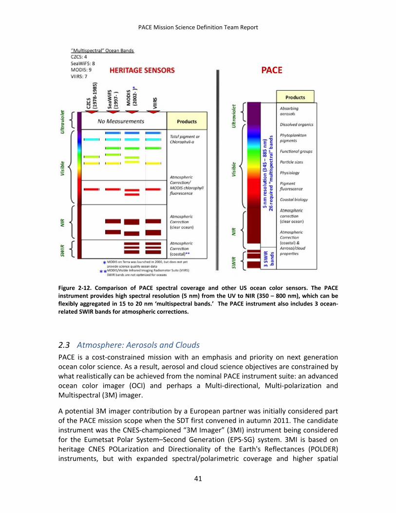
PACE Mission Science Definition Team Report
Figure 2-12. Comparison of PACE spectral coverage and other US ocean color sensors. The PACE instrument provides high spectral resolution (5 nm) from the UV to NIR (350 – 800 nm), which can be flexibly aggregated in 15 to 20 nm ‘multispectral bands.’ The PACE instrument also includes 3 ocean-related SWIR bands for atmospheric corrections.
2.3 Atmosphere: Aerosols and Clouds PACE is a cost-constrained mission with an emphasis and priority on next generation ocean color science. As a result, aerosol and cloud science objectives are constrained by what realistically can be achieved from the nominal PACE instrument suite: an advanced ocean color imager (OCI) and perhaps a Multi-directional, Multi-polarization and Multispectral (3M) imager.
A potential 3M imager contribution by a European partner was initially considered part of the PACE mission scope when the SDT first convened in autumn 2011. The candidate instrument was the CNES-championed “3M Imager” (3MI) instrument being considered for the Eumetsat Polar System–Second Generation (EPS-SG) system. 3MI is based on heritage CNES POLarization and Directionality of the Earth's Reflectances (POLDER) instruments, but with expanded spectral/polarimetric coverage and higher spatial
41
PACE Mission Science Definition Team Report
resolution. In March 2012, ESA decided to further consider 3MI as part of the EPS-SG. We do not know if a polarimeter will be included in the PACE mission at this time. However, because of the unique information that a 3M instrument provides for aerosol/cloud science as well as incomplete knowledge regarding PACE mission costs for flying OCI alone, the PACE SDT decided to continue to include in this report a discussion of a 3MI-like instrument and related science capabilities (“Goal” science as discussed below). Unless otherwise stated, further mention of a 3M imager will refer to the 3MI instrument as a baseline.
We note that NASA received draft white papers from the ACE SDT in 2010 making the recommendation for advanced polarimetric measurements in the context of ACE mission science. The PACE SDT did not have the charter or time to re-evaluate ACE recommendations. Therefore, the present report’s emphasis on 3MI-like capabilities should be considered together with the ACE document when/if NASA considers flight opportunities for a polarimeter.
ACE Context
To provide scientific context for PACE, we briefly summarize the Aerosol/Cloud/Ecosystems (ACE) science objectives and instrument complement as determined by the ACE aerosol and cloud working groups (see the ACE draft white paper and ACE SDT presentations at: http://dsm.gsfc.nasa.gov/ace/library.html). Sections 2.3.1 and 2.3.2 elaborate on that science, and discuss what can be achieved within the constraints of the more limited PACE instrument suite.
At the highest level, the Decadal Survey ACE mission aerosol and cloud discipline science objectives are to (1) decrease the uncertainty in aerosol forcing as a component of climate change, (2) quantify the role of aerosols in cloud formation and link aerosol changes to the modification of cloud properties and precipitation, and (3) improve the understanding of cloud feedback processes, all with the aim of improving climate prediction. The mission conceived in draft white papers by the ACE aerosol and cloud science working groups is a multi-sensor/multi-platform mission that includes (1) multichannel microwave*, submillimeter*, infrared*, visible and near-infrared (VNIR)-SWIR, and near-UV imaging, (2) an advanced multi-angle/multispectral polarimetric imager, (3) a high-spectral-resolution lidar, and (4) a dual-wavelength Doppler cloud radar [* indicates instrument may be called for in the Decadal Survey text but is not explicitly part of the ACE top-level summary]. The fusion of these data would make it possible to retrieve many cloud and aerosol properties that cannot be determined from current satellites, or are currently retrieved with large uncertainties. Examples of these properties include the vertical distributions of cloud and precipitation water and ice content, multiple moments of cloud and aerosol particle size distributions, aerosol morphology and refractive index, and vertical distribution of aerosol single scattering albedo and number concentration. More accurate knowledge of microphysical property profiles of such parameters is critical to furthering our understanding of aerosol forcing, aerosol transport, cloud processes, and cloud-aerosol interactions that limit our
42
PACE Mission Science Definition Team Report
understanding of the current climate and its response to an imposed forcing and consequently our ability to predict climate change. Details of the science and instrument requirements, as well as summary Science Traceability Matrices, are provided for aerosols and clouds primarily in Chapters 1 and 2, respectively, of the ACE draft white paper and also in the November 2010 progress report presentations (http://dsm.gsfc.nasa.gov/ace/library.html).
The PACE mission provides a subset of the ACE multispectral imaging capability with OCI (near-UV through the SWIR). Likewise, a PACE polarimeter based on 3MI would have a subset of ACE polarimetric imaging capabilities (see draft ACE aerosol white paper). Regardless, a mission relying only on solar reflectance measurements, even with polarization capabilities, will have limited information about the vertical structure of aerosol and cloud microphysical properties or hydrological cycle/precipitation processes, and therefore will not significantly advance our understanding of the indirect effects that tie these two science disciplines together. However, the OCI imager is expected to provide aerosol retrievals nominally comparable to MODIS/VIIRS and OMI (section 2.3.1) and, with some augmentation, a subset of cloud products from MODIS and VIIRS (section 2.3.2). If flown for PACE, a 3M polarimeter will provide advanced aerosol and cloud capabilities compared with POLDER, as described in sections 2.3.1 and 2.3.2.
Not all of the important cloud and aerosol properties and related processes/interactions can be determined adequately from space. Therefore, the aerosol-cloud portion of the ACE white paper documents also recognized the important role for suborbital measurements (i.e., ground-based and aircraft), which extends beyond satellite validation alone, and thus becomes a fundamental part of the mission design (Chapter 6 and 10 of the ACE draft white paper). Aspects of these requirements for the PACE instrument complement are discussed in sections 4.6.2 and 4.6.3.
Atmosphere Mission Requirement Categories
Two categories of atmosphere requirements are used throughout this report:
1. Threshold (T) requirements will fulfill the threshold atmospheric science question, and provide products that are critically needed. These products are obtained from the augmented OCI imager (OCI+) as described below and in section 3.3. Specifically, threshold products will:
• To the extent possible, continue climate records for aerosol and cloud products generated from the EOS heritage MODIS imager, as called out in the document titled, “Responding to the Challenge of Climate and Environmental Change: NASA’s Plan for a Climate-Centric Architecture for Earth Observations and Applications from Space,” June 2010. These
43
PACE Mission Science Definition Team Report
continuity requirements are also relevant for some aerosol/cloud data records from VIIRS and OMI products.
• Contribute additional information to the success of the primary mission objective, e.g., provision of sufficient cloud detection/screening to achieve required objectives for ocean color, aerosol, and other PACE clear-sky retrieval science.
• Provide novel cloud retrieval enhancements with unique OCI+ capabilities.
2. Goal (G) requirements will fulfill the goal atmospheric science questions, will enable the PACE mission to have advanced capabilities for the monitoring and understanding of aerosol and clouds, and will be linked to 3M and OCI+ instrument observations. Goal products will:
• Complement data records of aerosol and cloud variables observed by heritage sensors (POLDER, MISR).
• Contribute to the advance of aerosol and cloud research through provision of higher spatial resolution and/or new or enhanced cloud parameters from spectral capabilities not currently available from any existing or past mission.
These definitions specifically apply to the nominal retrieved product accuracies in the tables of sections. 2.3.1 and 2.3.2, and to the atmosphere instrument requirements given in section 3.3.
Atmosphere Science Questions (ASQs)
Relative to ACE, PACE atmospheric science questions are quite limited. The following questions are categorized as requiring atmosphere threshold or goal instrument capabilities:
ASQ-1: In combination with data records that were begun with heritage/existing imagers, what are the long-term changes in aerosol and cloud properties that can be continued with PACE and how are these properties correlated with interannual climate oscillations?
Threshold Science Question: requires OCI+.
A number of imager-based aerosol and cloud data records were initiated during the EOS era with MODIS. It is expected that the MODIS aerosol data records can likely be continued with VIIRS on the National Polar-orbiting Partnership and Joint Polar Satellite System-1 (JPSS-1). The PACE OCI imager with spectral augmentation (OCI+, described in
44
PACE Mission Science Definition Team Report
Table 3-4) will also have the inherent measurement capability to continue MODIS aerosol data records (see Table 2-1) and a subset of cloud properties. For low cloud properties specifically, both VIIRS and OCI+ can likely continue important MODIS cloud data records (OCI+ retrieval capabilities given in Table 2-3). Trend detection and quantification require long-term data records based on well characterized and radiometrically stable imagers. While trend detection depends on the size of the temporal/spatial domain, as well as natural variability, multi-decadal records are typically required. It is therefore critical to take optimal advantage of all imagers that are capable of providing continuity. In addition to helping determine statistically significant trends (global and regional), PACE can be used to improve the quantification and understanding of correlations between key interannual climate oscillations (e.g., El Nino/Southern Oscillation [ENSO]) and aerosol and cloud properties, which, in turn, provides a higher-level metric for assessing climate model performance.
ASQ-2: How do aerosols and their perturbations from nominal background amounts/types affect liquid water boundary layer cloud macrophysical, microphysical, and optical properties?
Goal Science Question: requires OCI+ with 250 m imagery in selected spectral channels (see section 2.3.2.2). A 3M imager would provide significant additional benefits (see section 2.3.2.3).
Sub-polar boundary layer and other low-level clouds have a large net radiative cooling effect due to their significant reflection of solar radiation, but relatively small thermal contrast with the surface. Climate simulations suggest a strong cloud radiative feedback, as boundary layer clouds respond to changes in the large-scale subsidence rate, but this response varies widely amongst climate models and hence is a large source of uncertainty in global cloud feedback and climate sensitivity [Bony et al., 2006]. Estimates of aerosol effects on clouds are also highly sensitive to the boundary-layer cloud representation in climate models [Forster et al., 2007].
Pathways with which aerosols can influence boundary-layer clouds include the first and second aerosol indirect effects from cloud condensation nuclei (CCN) perturbations (radiative and cloud water perturbations, respectively, e.g., Wilcox et al. [2010]) and the semi-direct effect (absorbing aerosol modifying thermodynamics/dynamics, e.g., Johnson et al. [2004]; Persad et al. [2012]).
Combined high-resolution imagery and 3M observations will allow for a more complete description of cloud microphysics than is currently available, including information regarding the uppermost cloud effective radius and effective variance from polarimetric measurements versus the deeper weighting from total radiance SWIR measurements. It is inherently difficult to separate aerosol from dynamic/thermodynamic induced cloud perturbations. The PACE mission and the aerosol data assimilation system (section 5.3.1) can help separate the two influences. The SDT notes that PACE will not be able to
45
PACE Mission Science Definition Team Report
identify and analyze aerosol-induced precipitation perturbations necessary to fully understand and quantify indirect mechanisms without an ACE-like radar; nor will PACE have access to aerosol extinction information adjacent to cloud boundaries without a lidar (see draft ACE white paper for complete discussion). However, the synergy of high spatial resolution imagery, along with improved spectral/spatial resolution 3M observations, will be unique for studying how cloud macrophysical structures and microphysical properties relate to local and regional thermodynamic conditions. Analysis of liquid cloud droplet size distribution moments will contribute to our understanding of how dynamics and radiation can force these extended cloud systems.
ASQ-3: How do clouds affect aerosol properties in regions near cloud boundaries?
Goal Science Question: requires OCI+ with 250 m imagery in selected spectral channels (see section 3.3) and a 3M imager.
In order to correctly assess the direct and indirect aerosol radiative forcings and their uncertainties, it is essential to understand and quantify the variability of aerosol properties in the vicinity of clouds. This is especially important because about half of all cloud-free pixels are closer than 5 km to low boundary layer clouds [Varnai and Marshak, 2011]. Also, aerosol properties are substantially different in large cloud-free and partly cloudy regions [Koren et al., 2007], and there is a strong correlation between aerosol optical depth and cloud cover (e.g., Loeb and Manalo-Smith, [2005]). However, the interpretation of satellite aerosol observations is particularly challenging in partly cloudy environments.
Combined high resolution imagery and 3M observations will allow for a more complete description of the transition zone between cloudy and clear air. The transition zone is a region of strong aerosol-cloud interactions where aerosol particles humidify and swell, while cloud drops evaporate and shrink, and vice versa [Koren et al., 2009]. This area complicates estimates of aerosol radiative forcing—excluding aerosols near clouds will dramatically reduce the database and underestimates the forcing, while including them may overestimate it because of unaccounted cloud contamination. Multi-angular polarized measurements will help to separate cloud contamination from aerosol hydroscopic growth. We note, however, that PACE will not enable full understanding of near-cloud behavior of aerosols without a lidar. Nevertheless, the synergy of high spatial resolution imagery, along with improved spectral/spatial resolution 3M observations, will be unique for studying the effects of clouds on aerosol properties and the uncertainties in the direct and indirect aerosol radiative forcings.
ASQ-4: What are the magnitudes and trends of Direct Aerosol Radiative Forcing (DARF), and the anthropogenic component of DARF?
46
PACE Mission Science Definition Team Report
Goal Science Question: requires the capabilities of an ACE-class 3M imager, with the aim of reducing the uncertainties in global and regional aerosol forcing components, so the resulting uncertainties are comparable to the other climate forcing factors in the Inter-governmental Panel on Climate Change (IPCC) assessment. Further details of the scientific motivations are given in section 2.3.1.1 below, and in the draft ACE white paper.
ASQ-5 (also discussed in Ocean SQ-4, see 2.2.1.4 for further details): How do aerosols influence ocean ecosystems and biogeochemical cycles?
Goal Science Question: requires 3M imager.
Dust-borne aerosol can contain iron, some of which is biologically available and may be responsible for significant primary production in high nutrient, low chlorophyll marine environments. ASQ-3 includes the following specifics: How does the transport and deposition of dust aerosol affect the productivity of iron-limited waters? What is the ultimate fertilization impact of individual dust sources?
A "goal" instrument with 3M measurements including SWIR spectral channels similar to 3MI will provide a unique capability for detecting coarse mode dust aerosols and important optical properties (optical depth, complex index of refraction, height information) that are not possible with OCI or heritage sensors. 3M observations can therefore provide important information regarding fertilization of iron-limited waters, such as the southern oceans, equatorial Pacific, and subarctic Pacific. While observations by themselves could be used to make some assessment of sources and deposition by quantifying changes in aerosol optical depth during transport, the observations are better utilized in conjunction with an aerosol data assimilation system (see section 5.3.1), providing improved quantification of dust sources, transport, and deposition.
2.3.1 Aerosols This section describes possible science objectives for the PACE mission.
2.3.1.1 Aerosol Optical Depth and Aerosol Type Direct aerosol radiative forcing (DARF) remains a leading contributor to climate prediction uncertainty [IPCC, 2007]. Calculations suggest that instantaneous, mid-visible aerosol optical depth (AOD) measurement accuracy of about 0.02 is typically required under cloud-free conditions to constrain DARF to approximately 1 Wm-2 [Mishchenko et al., 2004; McComiskey et al., 2008; CCSP, 2009], whereas the corresponding uncertainties in the current global AOD products from MISR and MODIS are 0.03 or
47
PACE Mission Science Definition Team Report
larger over dark water, and 0.05 or larger over land [Kahn et al., 2010; Levy et al., 2010; Remer et al., 2005]. However, to properly account for DARF, the capability of quantifying aerosols above clouds is also necessary, and is beginning to be explored by current sensors [Waquet et al., 2009; Torres et al., 2011].
Theoretical DARF sensitivity analysis also identifies aerosol type, especially particle single-scattering albedo (SSA), as the other leading factor in most situations, as particularly important for determining radiative forcing over land surfaces and clouds, and requiring an instantaneous constraint of about 0.02, though varying with other factors, such as AOD and surface albedo [McComiskey et al., 2008; Loeb and Su, 2010]. Reducing retrieved AOD uncertainties themselves is linked to obtaining better constraints on aerosol microphysical models, and microphysical information is also key to improving estimates of aerosol material fluxes, deposition, and other environmental impacts.
Aerosol-type-retrieval capabilities for the single-viewing MODIS amount to obtaining the fine/coarse ratio over water, with limited constraints on the sizes of the fine and coarse components [Remer et al., 2008]. Over land, there is essentially no particle property information, and AOD is retrieved from MODIS based on an aerosol type that is assumed from climatology [Levy et al., 2010]. For the multi-angle, radiance-intensity-only MISR instrument, three-to-five bins in aerosol size, two-to-four bins in SSA, and spherical vs. non-spherical AOD fraction can be distinguished under good retrieval conditions (i.e., provided the total column, mid-visible AOD exceeds about 0.15 or 0.2, and the scene is reasonably cloud and ice-free) [Kahn et al., 2010]. MODIS provides global coverage every two days, and MISR about once per week, both with 250 m to 1 km pixel resolution, depending on spectral channel (with 10-20 km aggregated level-2 pixels for the current operational versions of the products).
The hyperspectral single-viewing OMI instrument suffers from a large pixel size (13x24 km) that introduces uncertainty to the aerosol retrieval from sub-pixel clouds. However, OMI’s extension of spectral range into the ultraviolet (UV) introduces sensitivity to aerosol absorption that MODIS and MISR do not have [Zubko et al., 2007]. Properly exploited, this sensitivity can provide added information on particle absorption properties and aerosol type [Torres et al., 2007] and enables aerosol retrieval capability above clouds [Torres et al., 2011].
Polarization can increase the sensitivity of top-of-atmosphere (TOA) remote sensing observations to AOD, as well as particle size, shape, index of refraction, and SSA, and allows for retrievals under a broader range of observing conditions [Mishchenko and Travis, 1997a; Hasekamp and Landgraf, 2005; Waquet et al., 2009a; Knobelspiesse et al., 2012], including aerosols above clouds [Waquet et al., 2009b; Knobelspiesse et al., 2011].
Such added advantages of polarization have been demonstrated in analyses of real TOA data obtained by the POLDER instruments onboard the ADEOS mission, the ADEOS-2
48
PACE Mission Science Definition Team Report
mission, and the PARASOL mission [e.g., Bréon and Goloub, 1998; Herman et al., 2005; Gérard et al., 2005]. The PARASOL/POLDER instrument has multi-spectral, multi-angle polarimetric capabilities, with 6 spectral bands (3 polarized) and up to 16 viewing directions. PARASOL/POLDER provides global coverage every two days, with 6 km sub-spacecraft spatial resolution. The operational PARASOL/POLDER aerosol product includes fine/coarse differentiated AOD over water and fine component AOD over land [Tanré et al., 2011]. Also, coarse-mode spherical vs. non-spherical components are distinguished over water [Herman et al., 2005]. However, the current PARASOL algorithm uses a MODIS-like retrieval concept, oriented toward rapid operational processing. Several recent studies demonstrate the possibility of deriving a significantly extended set of aerosol parameters by implementing iterative radiative transfer calculations in the retrieval. For example, Hasekamp et al. [2011] estimate the Degrees Of Freedom for Signal (DOFS) of PARASOL/POLDER observations to range between 5 and 12, depending on the geometry of the observations; they demonstrate the possibility of retrieving refractive index and single scattering albedo from PARASOL/POLDER observations over ocean, in addition to AOD and Angström coefficient, with accuracy comparable to AERONET. They also demonstrate a factor-of-two improvement for the AOD retrieval, and a reduction in the mean difference between the PARASOL/POLDER and AERONET Angström Exponents from 0.15 to 0.02, when the multi-angle polarization capability is introduced into the retrieval algorithm. And Dubovik et al. [2011] describe an algorithm for deriving aerosol spectral AOD, complex index of refraction and SSA along with surface properties from PARASOL/POLDER observations over reflective land surfaces. The recent sensitivity study by Kokhanovsky et al. [2010] supports these results, demonstrating the value of multi-angle polarimetric observations for retrieving AOD and aerosol type information.
Nevertheless, some PARASOL/POLDER aerosol products, such as the complex refractive index, do not meet the requisite aerosol accuracy requirement for assessing aerosol effects on climate [Knobelspiesse et al., 2012]. So a substantial next step in constraining direct aerosol radiative forcing of climate, as well as other applications, would be to fly an advanced polarimeter to monitor AOD and aerosol microphysical properties globally, to combine these with detailed, suborbital measurements of the aerosol microphysical properties, and use the result to constrain climate models [e.g., Kahn, 2011].
The requisite set of aerosol macro- and micro-physical parameters is listed in Table 2-1 (based on the draft version of the ACE white paper). The corresponding retrieval accuracies formulated for reliable quantification of the direct and indirect aerosol effect on climate [see also Mishchenko et al., 2004] are shown as well, together with some retrieval estimates for the OCI and OCI+ instrument configurations. The retrieval estimates for the 3MI instrument discussed in section 2.3.1.3 are also provided in Table 2-1. The atmosphere threshold OCI+ instrument is intended for MODIS aerosol data record continuity and is not able to provide enough information to significantly advance our understanding of aerosols’ effect on climate (examples of climate-related applications for the ACE aerosol requirements are given in Table 2-2. However,
49
PACE Mission Science Definition Team Report
depending on the instrument design, all or a limited subset of these parameters can be retrieved from data obtained by a polarimeter. Real-world retrieval accuracies will depend on instrument factors, such as the accuracy of polarimetric and radiometric measurements, the number of polarization-sensitive spectral channels and their total spectral range, and the number and range of view angles [Mishchenko and Travis 1997a,b; Mishchenko et al., 1997; Hasekamp and Landgraf, 2007; Knobelspiesse et al., 2012], as well as pixel resolution, spatial coverage, and model errors (heterogeneity, forward model assumptions, ancillary data sources, etc.), which vary with retrieval conditions.
50
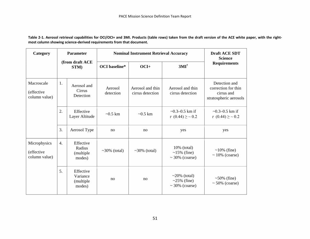
PACE Mission Science Definition Team Report
Table 2-1. Aerosol retrieval capabilities for OCI/OCI+ and 3MI. Products (table rows) taken from the draft version of the ACE white paper, with the right-most column showing science-derived requirements from that document.
Category Parameter
(from draft ACE STM)
Nominal Instrument Retrieval Accuracy Draft ACE SDT Science
Requirements OCI baseline* OCI+ 3MI†
Macroscale
(effective column value)
1. Aerosol and Cirrus
Detection
Aerosol detection
Aerosol and thin cirrus detection
Aerosol and thin cirrus detection
Detection and correction for thin
cirrus and stratospheric aerosols
2. Effective Layer Altitude ~0.5 km ~0.5 km ~0.3–0.5 km if
τ (0.44) ≥ ~ 0.2 ~0.3–0.5 km if
τ (0.44) ≥ ~ 0.2
3. Aerosol Type no no yes yes
Microphysics
(effective column value)
4. Effective Radius
(multiple modes)
~30% (total) ~30% (total) 10% (total) ~15% (fine)
~ 30% (coarse)
~10% (fine) ~ 10% (coarse)
5. Effective Variance (multiple modes)
no no ~20% (total) ~25% (fine)
~ 30% (coarse)
~50% (fine) ~ 50% (coarse)
51
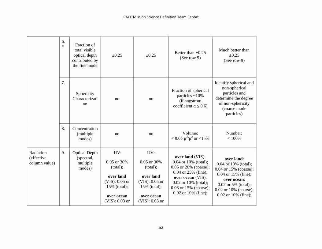
PACE Mission Science Definition Team Report
6. * Fraction of
total visible optical depth
contributed by the fine mode
±0.25 ±0.25 Better than ±0.25 (See row 9)
Much better than ±0.25
(See row 9)
7.
Sphericity Characterizati
on no no
Fraction of spherical particles ~10%
(if angstrom coefficient α ≤ 0.6)
Identify spherical and non-spherical particles and
determine the degree of non-sphericity
(coarse mode particles)
8. Concentration (multiple modes)
no no Volume: < 0.05 μ3/μ2 or <15%
Number: < 100%
Radiation (effective column value)
9. Optical Depth (spectral, multiple modes)
UV:
0.05 or 30% (total);
over land (VIS): 0.05 or 15% (total);
over ocean (VIS): 0.03 or
UV:
0.05 or 30% (total);
over land (VIS): 0.05 or 15% (total);
over ocean (VIS): 0.03 or
over land (VIS): 0.04 or 10% (total);
0.05 or 20% (coarse); 0.04 or 25% (fine); over ocean (VIS):
0.02 or 10% (total); 0.03 or 15% (coarse); 0.02 or 10% (fine);
over land: 0.04 or 10% (total);
0.04 or 15% (coarse); 0.04 or 15% (fine);
over ocean: 0.02 or 5% (total);
0.02 or 10% (coarse); 0.02 or 10% (fine);
52
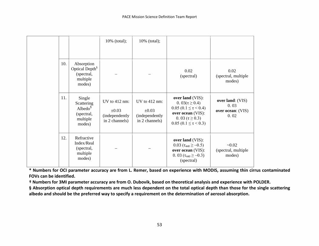
PACE Mission Science Definition Team Report
10% (total);
10% (total);
10. Absorption Optical Depth§
(spectral, multiple modes)
– – 0.02
(spectral)
0.02 (spectral, multiple
modes)
11. Single Scattering Albedo§ (spectral, multiple modes)
UV to 412 nm:
±0.03 (independently in 2 channels)
UV to 412 nm:
±0.03 (independently in 2 channels)
over land (VIS): 0. 03(τ ≥ 0.4)
0.05 (0.1 ≤ τ < 0.4) over ocean (VIS):
0. 03 (τ ≥ 0.3) 0.05 (0.1 ≤ τ < 0.3)
over land: (VIS) 0. 03
over ocean: (VIS) 0. 02
12. Refractive Index/Real (spectral, multiple modes)
– –
over land (VIS): 0.03 (τ440 ≥ ~0.5)
over ocean (VIS): 0. 03 (τ440 ≥ ~0.3)
(spectral)
~0.02 (spectral, multiple
modes)
* Numbers for OCI parameter accuracy are from L. Remer, based on experience with MODIS, assuming thin cirrus contaminated FOVs can be identified. † Numbers for 3MI parameter accuracy are from O. Dubovik, based on theoretical analysis and experience with POLDER. § Absorption optical depth requirements are much less dependent on the total optical depth than those for the single scattering albedo and should be the preferred way to specify a requirement on the determination of aerosol absorption.
53
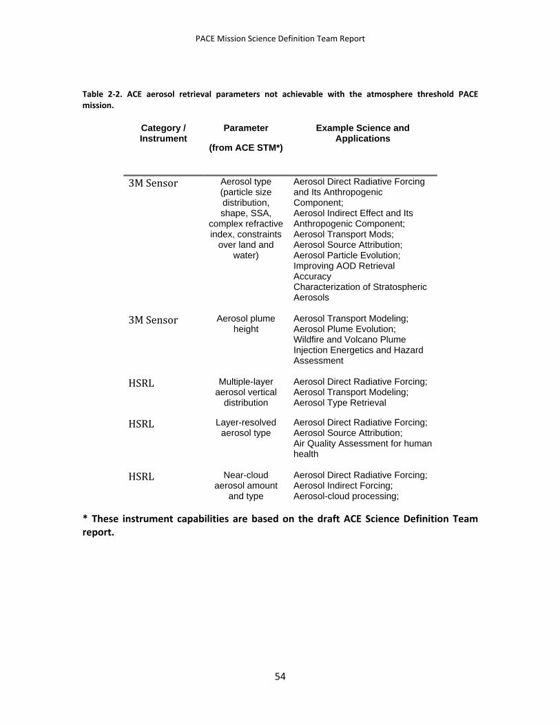
PACE Mission Science Definition Team Report
Table 2-2. ACE aerosol retrieval parameters not achievable with the atmosphere threshold PACE mission.
Category / Instrument
Parameter
(from ACE STM*)
Example Science and Applications
3M Sensor Aerosol type (particle size distribution, shape, SSA,
complex refractive index, constraints
over land and water)
Aerosol Direct Radiative Forcing and Its Anthropogenic Component; Aerosol Indirect Effect and Its Anthropogenic Component; Aerosol Transport Mods; Aerosol Source Attribution; Aerosol Particle Evolution; Improving AOD Retrieval Accuracy Characterization of Stratospheric Aerosols
3M Sensor Aerosol plume height
Aerosol Transport Modeling; Aerosol Plume Evolution; Wildfire and Volcano Plume Injection Energetics and Hazard Assessment
HSRL Multiple-layer aerosol vertical
distribution
Aerosol Direct Radiative Forcing; Aerosol Transport Modeling; Aerosol Type Retrieval
HSRL Layer-resolved aerosol type
Aerosol Direct Radiative Forcing; Aerosol Source Attribution; Air Quality Assessment for human health
HSRL Near-cloud aerosol amount
and type
Aerosol Direct Radiative Forcing; Aerosol Indirect Forcing; Aerosol-cloud processing;
* These instrument capabilities are based on the draft ACE Science Definition Team report.
54
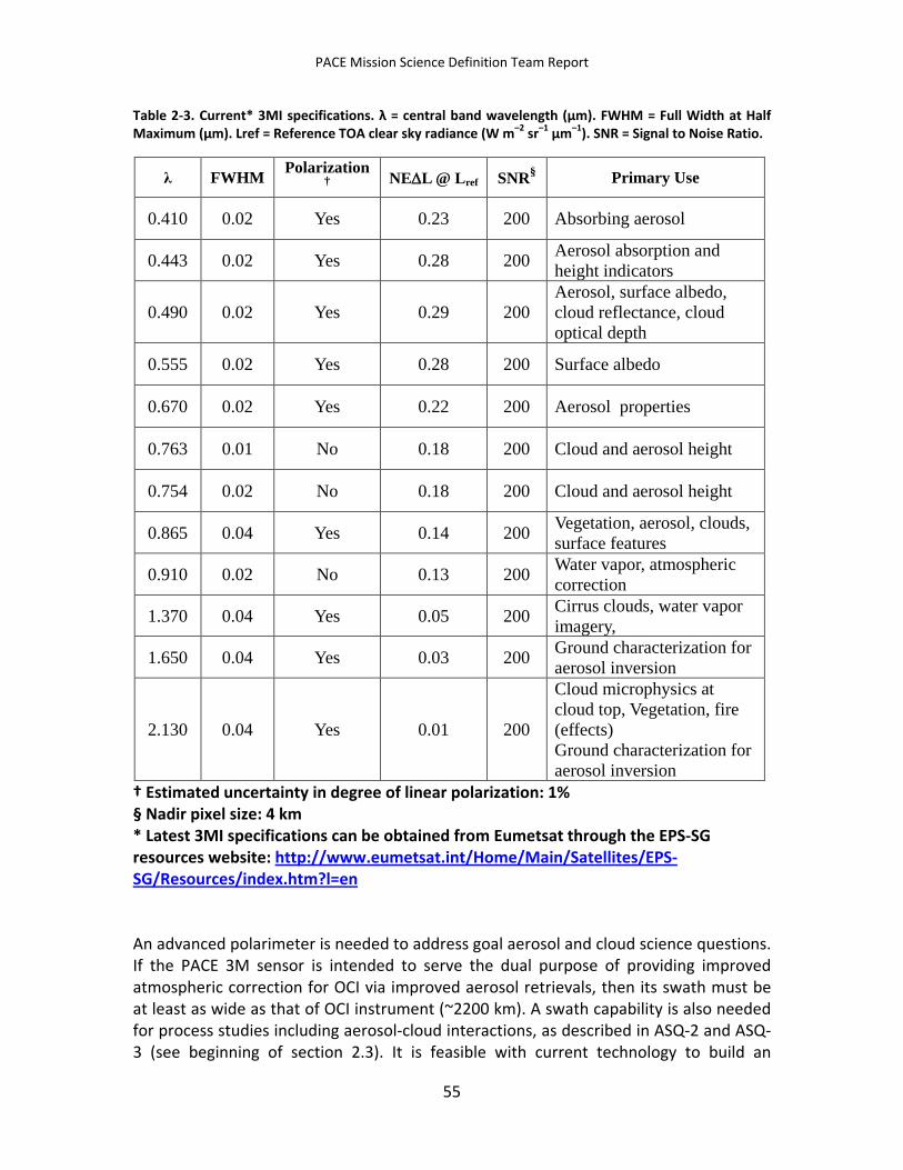
PACE Mission Science Definition Team Report
Table 2-3. Current* 3MI specifications. λ = central band wavelength (μm). FWHM = Full Width at Half Maximum (μm). Lref = Reference TOA clear sky radiance (W m–2 sr–1 μm–1). SNR = Signal to Noise Ratio.
λ FWHM Polarization† NE∆L @ Lref SNR§ Primary Use
0.410 0.02 Yes 0.23 200 Absorbing aerosol
0.443 0.02 Yes 0.28 200 Aerosol absorption and height indicators
0.490 0.02 Yes 0.29 200 Aerosol, surface albedo, cloud reflectance, cloud optical depth
0.555 0.02 Yes 0.28 200 Surface albedo
0.670 0.02 Yes 0.22 200 Aerosol properties
0.763 0.01 No 0.18 200 Cloud and aerosol height
0.754 0.02 No 0.18 200 Cloud and aerosol height
0.865 0.04 Yes 0.14 200 Vegetation, aerosol, clouds, surface features
0.910 0.02 No 0.13 200 Water vapor, atmospheric correction
1.370 0.04 Yes 0.05 200 Cirrus clouds, water vapor imagery,
1.650 0.04 Yes 0.03 200 Ground characterization for aerosol inversion
2.130 0.04 Yes 0.01 200
Cloud microphysics at cloud top, Vegetation, fire (effects) Ground characterization for aerosol inversion
† Estimated uncertainty in degree of linear polarization: 1% § Nadir pixel size: 4 km * Latest 3MI specifications can be obtained from Eumetsat through the EPS-SG resources website: http://www.eumetsat.int/Home/Main/Satellites/EPS-SG/Resources/index.htm?l=en An advanced polarimeter is needed to address goal aerosol and cloud science questions. If the PACE 3M sensor is intended to serve the dual purpose of providing improved atmospheric correction for OCI via improved aerosol retrievals, then its swath must be at least as wide as that of OCI instrument (~2200 km). A swath capability is also needed for process studies including aerosol-cloud interactions, as described in ASQ-2 and ASQ-3 (see beginning of section 2.3). It is feasible with current technology to build an
55
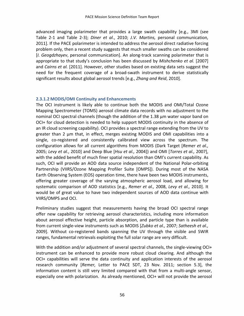
PACE Mission Science Definition Team Report
advanced imaging polarimeter that provides a large swath capability [e.g., 3MI (see Table 2-1 and Table 2-3); Diner et al., 2010; J.V. Martins, personal communication, 2011]. If the PACE polarimeter is intended to address the aerosol direct radiative forcing problem only, then a recent study suggests that much smaller swaths can be considered [I. Geogdzhayev, personal communication]. An along-track scanning polarimeter that is appropriate to that study’s conclusion has been discussed by Mishchenko et al. [2007] and Cairns et al. [2011]. However, other studies based on existing data sets suggest the need for the frequent coverage of a broad-swath instrument to derive statistically significant results about global aerosol trends [e.g., Zhang and Reid, 2010].
2.3.1.2 MODIS/OMI Continuity and Enhancements The OCI instrument is likely able to continue both the MODIS and OMI/Total Ozone Mapping Spectrometer (TOMS) aerosol climate data records with no adjustment to the nominal OCI spectral channels (though the addition of the 1.38 µm water vapor band on OCI+ for cloud detection is needed to help support MODIS continuity in the absence of an IR cloud screening capability). OCI provides a spectral range extending from the UV to greater than 2 µm that, in effect, merges existing MODIS and OMI capabilities into a single, co-registered and consistently calibrated view across the spectrum. The configuration allows for all current algorithms from MODIS (Dark Target [Remer et al., 2005; Levy et al., 2010] and Deep Blue [Hsu et al., 2004]) and OMI [Torres et al., 2007], with the added benefit of much finer spatial resolution than OMI’s current capability. As such, OCI will provide an AOD data source independent of the National Polar-orbiting Partnership (VIIRS/Ozone Mapping Profiler Suite [OMPS]). During most of the NASA Earth Observing System (EOS) operation time, there have been two MODIS instruments, offering greater coverage of the varying atmospheric aerosol load, and allowing for systematic comparison of AOD statistics [e.g., Remer et al., 2008, Levy et al., 2010]. It would be of great value to have two independent sources of AOD data continue with VIIRS/OMPS and OCI.
Preliminary studies suggest that measurements having the broad OCI spectral range offer new capability for retrieving aerosol characteristics, including more information about aerosol effective height, particle absorption, and particle type than is available from current single-view instruments such as MODIS [Zubko et al., 2007; Satheesh et al., 2009]. Without co-registered bands spanning the UV through the visible and SWIR ranges, fundamental retrievals exploiting the full solar range are very difficult.
With the addition and/or adjustment of several spectral channels, the single-viewing OCI+ instrument can be enhanced to provide more robust cloud clearing. And although the OCI+ capabilities will serve the data continuity and application interests of the aerosol research community [Remer, Letter to PACE SDT, 23 Nov. 2011; section 5.3], the information content is still very limited compared with that from a multi-angle sensor, especially one with polarization. As already mentioned, OCI+ will not provide the aerosol
56
PACE Mission Science Definition Team Report
type information needed to advance current constraints on aerosol climate forcing (see Table 2-1 and related discussion above).
2.3.1.3 3MI Enhancements to PACE Aerosol Objectives The aerosol-related measurement capabilities, and therefore the aerosol-related objectives, of the PACE Mission would be substantially enhanced if the 3MI instrument—an advanced design based on POLDER—is incorporated into the payload.
Table 2-3 provides an overview of the 3MI measurement capabilities. The 3MI will improve upon the POLDER design in three areas: (1) more wavelength bands (12 wavelengths total, 9 with polarization) covering a wider spectral range (starting at 410 nm in the VIS, and including SWIR wavelengths up to 2130 nm), (2) higher spatial resolution (ground resolution of 4 km VIS and SWIR), and (3) wider swath (114° field-of-view, with 10 to 14 view angles per ground pixel). The wider spectral range and availability of polarimetric observations at most channels are expected to improve size distribution, particle shape, and especially complex index of refraction retrieval accuracy. The SWIR channels will improve the sensitivity to large and non-polarizing (non-spherical) particles. The additional 410 nm total and polarized reflectance channels will help reduce the altitude vs. single scattering albedo ambiguity, while also providing better aerosol absorption constraints at this wavelength. This should help distinguishing dust aerosol from clouds, providing improved short-wave flux and radiative forcing estimates. The extended spectral coverage will also improve surface albedo retrievals, allowing more complete shortwave aerosol forcing estimates. Finally, both the improved resolution and additional spectral channels will contribute to better cloud detection, reducing contamination by unresolved sub-pixel clouds, and also allowing for retrievals to be performed closer to aerosol/cloud boundaries, contributing to better observations of aerosol-cloud interactions. Estimated 3MI retrieval accuracies are shown for the set of aerosol parameters given in Table 2-1. Differences seen in this Table between the draft ACE and 3MI values can be attributed to the ACE column giving white paper science requirements, whereas the 3MI values are retrieval accuracies for the specific 3MI instrument design.
As already mentioned, real-world retrieval capabilities are determined by a combination of measurement and model error sources. To help resolve issues related to practical retrieval capabilities, the draft ACE document recommended appropriate polarimetric data to be collected and analyzed as part of a robust field program. This is discussed again in section 4.6.2 and in the following section.
2.3.1.4 Recommendations for Phase-A Studies While the POLDER instruments provided an extremely important and unique dataset, this and other reports have argued that advanced spaceborne 3M measurements are a
57
PACE Mission Science Definition Team Report
critical component to an observation strategy for making substantial progress in aerosol climate science and related applications. Such global polarimetric observations are still years away (EPS-SG or PACE ~2020, and post-2022 for ACE, according to current NASA Earth Science Division [ESD] plans). It will be extremely valuable to support Phase-A tasks that seek to better understand retrieval information content and uncertainties from synergistic algorithms using total radiance (OCI+) and polarimetric observations that would be feasible with a goal atmosphere science PACE mission.
Retrieval uncertainties can nominally be separated into two general categories. Measurement uncertainty includes radiometric and polarimetric error sources, in addition to other instrument error sources. The impact of measurement error can begin to be assessed once a forward radiative model is available (e.g., sensitivity and information content studies) or more quantitatively if an inverse algorithm is also available to correctly infer the impact of retrieval nonlinearities. Model uncertainties encompass forward radiative model error sources associated with physical assumptions and radiative calculations (e.g., spatial structure/heterogeneity, assumptions regarding physical quantities not directly sensed, ancillary data source errors, etc.) and as such are much more difficult to directly calculate. Depending on the scene, and the pixel resolution of the sensor, it is likely that either measurement or modeling errors could dominate instantaneous retrievals.
The following goal aerosol retrieval issues are recommended for further study during Phase-A:
• Assessment of model errors:
o Field observations: This can include existing data sets (e.g., Polarimeter Definition Experiment [PODEX], Jan-Feb. 2013) or additional field work that capitalizes on existing and new airborne polarimeters (Airborne Multiangle SpectroPolarimetric Imager [AirMSPI], Research Scanning Polarimeter [RSP], Portland Aerosol Characterization Study [PACS]), imagers, and lidars, as well as in situ and ground-based measurements. See section 4.6.2 for additional details. In particular, additional low-altitude characterization of land and ocean surface polarized bidirectional reflectance distribution functions (BRDFs) would be valuable in assessing modeling errors associated with surfaces.
o 3D studies: Generate realistic 3D aerosol fields and cloud fields (e.g., large eddy simulation [LES]) and apply a vector Monte Carlo radiative transfer code that can provide input to an appropriate aerosol retrieval code. The use of LES fields generated with and without the inclusion of aerosol indirect effects over a range of large scale dynamical backgrounds would be of particular value.
• In conjunction with the above studies, assess 3M measurement requirements (spectral, spatial, angular, polarimetric) needed to advance the full range of
58
PACE Mission Science Definition Team Report
PACE aerosol science questions (also see cloud recommendations in section 2.3.2, as well as ocean color atmospheric correction text). The nominal 3MI instrument, as well as aspects of draft ACE polarimeter measurement requirements, should be evaluated more fully.
• Observing System Simulation Experiment (OSSE): While the OSSE framework has traditionally been used to assess the impact of observations on numerical weather prediction, it can also be used to simulate observations for mission sampling studies and quantify errors in retrieval algorithms. We recommend Phase-A OSSEs based on atmospheric properties derived from a global Earth system model radiatively coupled with aerosols, running at a resolution of at least 10 km globally (global models are now capable of simulating realistic cloud and aerosol systems). Using climatological surface characteristics derived from EOS sensors, these simulations can use a comprehensive atmospheric and oceanic vector radiative transfer model to produce simulated top-of-the atmosphere reflectances as they would have been observed by PACE instruments. A close partnership between instrument and retrieval teams will enable parameterized observation errors to be added to these reflectances. The OSSEs would be useful in quantifying the impact of PACE measurements on aerosol (and cloud) forecast skills, increasing the effectiveness of atmospheric correction schemes for ocean color algorithms, helping guide the development of retrieval algorithms, and providing a tool for mission/instrument trade studies.
2.3.2 Clouds For context, we begin with an overview of the ACE cloud objectives. The overall objective of the ACE mission cloud working group is to advance the ability to observe and predict changes to the Earth’s hydrological cycle and energy balance in response to climate forcings, especially those changes associated with the effects of aerosol on clouds and precipitation [see ACE draft white paper at http://dsm.gsfc.nasa.gov/ace/library.html]. While it is important to continue observations begun with A-Train sensors that are, in part, expected to be extended by the EarthCARE mission (estimated launch in 2016), the ACE instrument suite would provide new information on cloud and precipitation microphysics (multiple moments of the size distribution) that are essential for better constraining cloud processes. In turn, this will ultimately help constrain cloud feedbacks which have been the tall pole in modeling intercomparison studies (e.g., Coupled Model Intercomparison Project Phase 3 [CMIP3]) and therefore for climate prediction [IPCC, 2007; Randall et al., 2007]. The physical processes that relate aerosols, clouds, and precipitation with atmospheric motion begin with the essential ability to infer vertical profiles of aerosol, cloud, and precipitation microphysical properties from measurements. It is this provision for new
59
PACE Mission Science Definition Team Report
microphysical information, vital for addressing climate science objectives in the coming decades, that differentiates ACE from predecessor missions.
Improving the ability to predict changes in the hydrological cycle and energy balance ultimately requires improving our understanding of the processes that generate clouds and precipitation, including interactions with aerosols. Much of the interaction between cloud, aerosol and precipitation occurs at the microphysical level, where cloud particle nucleation, growth, coalescence, and evaporation take place. Thus, in addition to traditional measurements of macrophysical (such as cloud-top-height) and radiative properties (e.g., cloud optical thickness, effective particle size) it was deemed critical that ACE obtain information on the microphysics of clouds, aerosols, and precipitation throughout the depth of the atmosphere.
In the broadest sense, the science goals of the ACE mission are to provide observations that answer the following science questions: (1) How do the macrophysical, microphysical, and radiative properties of clouds and precipitation change as a function of the thermodynamic and dynamic environment? (2) How do the distributions of these properties differ with changes in aerosol properties? More specifically, the ACE cloud science questions are categorized in terms of cloud morphology, microphysics/microphysical processes, and energetics. They are further subdivided according to cloud type (cirrus, deep convection, boundary layer and cumulus, mid-latitude frontal, and polar clouds), each with its own specific retrieval requirements.
Details of these science questions (see ACE white paper tables for each cloud type) and the set of geophysical parameters required to address the questions is beyond the scope of the present document. However a summary of the ACE cloud parameters is provided via the row entries in Tables 2-3 and 2-4. The reader is referred to the ACE white paper for further information including the retrieval requirements for each parameter.
For ACE, retrieval requirements were mapped to a set of technologically feasible measurements that supply the necessary information to retrieve the parameters to within the required accuracy. This approach resulted in a matrix that allows science requirements to be traced to measurement requirements via the geophysical parameters, i.e., a Science Traceability Matrix (STM). Because the nominal PACE mission measurement suite has already been defined, for pragmatic reasons we necessarily start with PACE measurements instead of the other way around. In principle, mapping PACE measurements to cloud retrieval capabilities could then be aligned with a subset of the ACE science objectives. However, mapping the PACE measurements into science objectives in the context of ACE is problematic because the passive measurements were closely tied with objectives that require the full ACE active and passive instrument suite.
Therefore, we focus the remaining text in section 2.3.2 on the geophysical parameters that are retrievable using the PACE instrument suite and partition the capabilities into those that allow for some level of data product continuity with existing NASA
60
PACE Mission Science Definition Team Report
instruments and/or provide for enhanced retrieval capabilities. It is understood that the rationale for data continuity and enhanced retrievals needs to be gauged in terms of broader NASA ESD programmatic efforts including the Suomi National Polar-orbiting Partnership/JPSS-1 and ACE.
Table 2-4 and Table 2-5 give a list of the geophysical parameters that were part of the ACE objectives, with the latter table listing those that are not possible (or at least not possible with sufficient accuracy) within the scope of the PACE mission. The cloud parameters are categorized according to macrophysics, microphysics, and radiation.
Establishing geophysical data continuity across multiple missions continues to be a challenge. Augmentation of the baseline OCI imager (referred to as OCI+, see section 3 for details) will allow for a subset of the cloud property retrievals available from MODIS and VIIRS. The subset is discussed in section 2.3.2.1; a list of the retrievals that are possible with OCI+ and their estimated accuracies are given in a column of Table 2-4. Notably absent from PACE is the capability for unambiguous continuity with cloud-top pressure/temperature height products from infrared imager observations. The possibilities for new capabilities are also discussed.
A 3MI-like polarimeter will allow for continuity of POLDER products, in addition to providing significant advancements in cloud property retrieval capabilities. Those capabilities are given as a separate column in Table 2-4; they include the synergy provided by collocated OCI+ observations when noted.
2.3.2.1 Cloud Product Continuity In the following, we discuss the impact of heritage instrument differences (MODIS vs. VIIRS) on cloud products and the extent to which an OCI imager can provide some level of heritage continuity. We note that without infrared channels, OCI cloud continuity is obviously applicable to daytime observations only.
2.3.2.1.1 Heritage Instruments The MODIS Terra and Aqua cloud products include cloudy Field of View (FOV) detection/masking and cloud products that include both cloud-top (temperature, pressure, effective emissivity) and optical/microphysical properties (thermodynamic phase, optical thickness, effective particle radius, water path, multilayer detection and other QA).
The VIIRS instrument has the capability to provide continuity for many of the MODIS cloud products, with the most notable exception being cloud-top properties. This is because VIIRS lacks several key spectral channels compared to MODIS (namely, 13.3-14.2 µm CO2 bands used for high cloud properties, but also a 7.3 µm water vapor band used in the MODIS Collection 6 IR-based cloud thermodynamic phase algorithm). As a
61
PACE Mission Science Definition Team Report
result, the cloud-top information content of MODIS observations is superior to VIIRS [Heidinger et al., 2010]. As discussed below, OCI observations in the A-band will be informative in their own right but are difficult to directly compare with infrared methods (with or without CO2 slicing capabilities). Therefore, PACE cannot provide continuity with either MODIS or VIIRS cloud-top data records. As mentioned below, VIIRS has chosen a longer wavelength position for the 2.1 µm window band, with implications for cloud effective particle radius continuity with MODIS.
As reference, an assessment of the MODIS cloud products has been undertaken by a number of investigators, including the MODIS algorithm team. The team has also participated in the continuing Global Energy and Water Cycle Experiment (GEWEX) cloud assessment study [e.g., Stubenrauch and Kinne, 2009; Stubenrauch et al., 2011, 2012]. While such assessments will continue, the uncertainties and/or issues for most of the cloud products are understood and have been documented. An assessment of cloud retrieval accuracies from a MODIS-like imager is given in the GEWEX cloud assessment [Stubenrauch et al., 2011, 2012]. Accuracies from this assessment and ACE working group documents have been used for appropriate parameters in Table 2-4.
2.3.2.1.2 Cloud Detection/Masking A previous study that looked into the removal of infrared (IR) measurements for daytime cloud detection [S. A. Ackerman, personal communication] generally found that:
1) A reduction in capability during winter over cold surfaces (IR was able to pick up the temperature contrast using thermal inversion tests with some combination of 11, 6.7 or 7.6 µm channels).
2) Infrared bands have proved particularly useful for high cloud detection. Split window infrared (IR) window measurements (or tri-spectral including 8.5 µm channel) can help with thin cirrus detection, including those that a 1.38 µm channel misses when water vapor loading is small.
3) Split window can also help with separating desert dust from cloud.
4) The cloud optical thickness detection limit over land is ~0.3 with IR observations; the detection limit is expected to increase without an IR capability. The detection limit may be similar to 0.3 over the ocean, though further analysis is needed.
Systematic daytime studies using MODIS and VIIRS cloud mask algorithms, with and without application of IR detection tests, are needed to quantify the reduction in skill as a function of cloud height and surface
62
PACE Mission Science Definition Team Report
2.3.2.1.3 Cloud Pressure Height There is inherent ambiguity in the meaning of cloud-top among various passive methods. Infrared retrievals, e.g., CO2 slicing or even IR window methods, give a radiative equivalent cloud-top, nominally at a penetration depth equivalent to a unit optical depth into the cloud (for a nadir view) for a cloud that is sufficiently optically thick [Holz et al., 2006, 2008].
Making use of the oxygen A-band absorption feature from an OCI imager (5 nm resolution, see section 3) provides another alternative to pressure height retrievals. Satellite heritage for such retrievals comes from the broader A-band channels on POLDER (10 and 40 nm) and the narrower MERIS channel (3.75 nm). To retrieve a so-called cloud apparent pressure, POLDER uses two spectral bands: a narrow (10 nm) and wide (40 nm) channel centered about the oxygen A-band (764 nm). In the case of very dark surface (over ocean), cloud apparent pressure is inferred from the ratio between the narrowband and broadband radiances, assuming that cloud optical thickness and cloud thermodynamic phase are determined from other POLDER channels [Buriez et al., 1997, Vanbauce et al., 2003]. Since the surface can be very bright over land at 764 nm (especially for vegetation), the inferred cloud pressure is corrected for the effect of the bright surface [Buriez et al., 1997]. The MERIS retrieval is based on the algorithm of Fischer et al. [1991a, 1991b, 1997].
Because of multiple scattering, the O2 in-cloud path absorption can be significant, relative to the above-cloud path. That is, the cloud cannot be modeled as an infinitesimally thin reflector located at the top of the cloud. As a result, the retrieved cloud pressure is always higher (lower in the atmosphere) than the Cloud-Top Pressure (CTP) obtained from IR retrievals. The difference between CTP and O2 pressure depends on the photon in-cloud path length distribution, which is a function of cloud optical and geometrical thicknesses, solar/view geometry, cloud type, and microphysics [Sneep et al., 2008; Ferlay et al., 2010]. The differences can be of the order of 70–90 hPa [Sneep et al., 2008]. The inferred O2 cloud pressure has been found to be much closer to the mid-cloud pressure (MCP) rather than CTP [Ferlay et al., 2010]. Similarly, the expected accuracy of the MERIS retrieval is >70 hPa for thin, high clouds but 30 hPa for low clouds [Fischer et al., 1997].
For low liquid clouds the O2-derived MCP tends to provide more reliable information on cloud location than CTP for two reasons. First, the IR based CTP retrievals suffer from a bias introduced by temperature inversion in the lower atmosphere that can only be accounted for by assuming a constant lapse rate [Minnis et al., 1992; Wu et al., 2008; Holz et al., 2008]. Second, the relatively limited vertical extent and large particle number concentrations (large extinction) contribute to a smaller difference between CTP and the O2 A-band derived MCP. As an example, a low cloud cumulus and stratocumulus validation study of MERIS retrievals over land showed root mean square (RMS) accuracies of about 24 hPa with a bias of ~22 hPa [Lindstrot et al., 2006]. However, much larger uncertainties are expected for high clouds, though the O2 pressure can carry potential information on cloud geometrical thickness [Ferlay et al., 2010]. Both
63
PACE Mission Science Definition Team Report
types of retrievals work well for a single layer clouds, or in the case of IR methods, a multilayer scene with an opaque upper-level cloud layer.
According to Preusker and Lindstrot [2009], calculations for MERIS of the sensitivity of CTP to geometrical thickness for single layers clouds that are optically thick and/or over a dark surface showed that a change in pressure height of 10 hPa is equivalent to a thickness change of 13 hPa. This translates to a 130 m uncertainty in cloud thickness giving rise to about 100 m and 200 m uncertainties in cloud height for low and high clouds, respectively. The same study also gives sensitivities of CTP to cloud optical thickness (~10%) and bright surfaces (especially problematic for optically thin clouds). An information content analysis for the A-band is also presented by Heidinger and Stephens [2000].
In order to avoid ambiguity on the meaning of cloud height, or cloud-top pressure height, the retrieved height from the O2 A-band channel will be discussed in terms of the MCP. For multilayer clouds, the effective MCP can be irrelevant or physically meaningless [e.g., Preusker and Lindstrot, 2009]. One way to detect and flag a multilayer cloud structure is by using the width of the photon path length distribution, or the standard deviation of O2 pressures derived from multi-angle observations (discussed further with respect to 3MI). A large standard deviation is a good indication of the multilayer cloud structure [Li and Min, 2010; Ferlay et al., 2010]. It is also possible that the synergistic use of a 940 nm OCI+ water vapor absorption channel can help diagnose multilayer scenes by providing a significantly different vertical weighting [Wind et al., 2010; Lindstrot et al., 2010]. While very challenging with the OCI 5 nm spectral resolution, use of the relatively weak O2- O2 absorption at 477 nm [Acarreta et al., 2004; Sneep et al., 2008] and the O2 B-band should also be explored for this purpose (see Joiner et al. [2010] for a similar approach using rotational Raman scattering).
While further study is needed, it should be noted that the higher spectral resolution of OCI compared to POLDER (10 nm) could provide the ability to sample different mean photon path lengths if the spectral dispersive element of OCI is aligned to sample both the high and low absorption regime of the O2 A-band structure. The resulting different weighting functions of two neighboring channels could potentially provide information on vertical cloud structure [Preusker et al., 2010]. The combination of a NIR water vapor absorption band or other oxygen bands (O2- O2, B-band) might also allow for additional retrieval information. Multiple A-band channels could also assist in multilayer detection for similar reasons, as discussed above. We emphasize that understanding the retrieval benefit from multiple A-band, water vapor, or other oxygen absorption channels requires Phase-A resources as noted in section 2.3.2.4.
In summary, the O2 A-band pressure height: (a) may be of limited use for high thin clouds, but can carry potential information on cloud geometrical thickness; and (b) is expected to be very useful for low cloud pressure retrievals, especially in regions where there are temperature inversions and where the geometrical thickness is small or well constrained.
64
PACE Mission Science Definition Team Report
2.3.2.1.4 Cloud Optical Thickness and Microphysics Knowledge of cloud microphysical properties is critical to understanding cloud radiation and cloud-aerosol processes. More generally, microphysical properties (phase, particle size) are tightly linked to cloud radiative properties, impact cloud lifecycle through glaciation and precipitation processes and may be subject to modification by aerosols. Continuity of cloud thermodynamic phase, effective particle size, and water path data records begun with the Advanced Very High Resolution Radiometer (AVHRR) and enhanced with MODIS will be only partially possible with the OCI imager.
Regarding effective radius, there is a significant change in the spectral location for a key VIIRS shortwave infrared band (from 2.13 µm to 2.25 µm) used for retrieving cloud effective particle radius that results in much less absorption for ice phase particles (factor of 3 decrease in co-albedo). The shift towards longer wavelengths is not necessarily without merit for phase detection, but with a significant increase in single scattering albedo, meaningful comparisons with the MODIS 2.13 µm window band are unlikely for ice clouds, due to both a reduction in sensitivity and changes in the vertical weighting through the cloud [Zhang et al., 2010]. The small increase in single scattering albedo in the VIIRS channel for liquid water clouds (14% decrease in co-albedo at re=12 µm, or an absorption decrease equivalent to ∆re ≈-1.6 µm) is unlikely to result in noticeable MODIS-VIIRS biases in heterogeneous clouds. However, PACE provides an opportunity to compare the microphysical records of both MODIS and VIIRS for identical pixel FOVs in this important SWIR band by augmenting the baseline OCI to include a 2.25 µm VIIRS channel (in addition to the 2.13 µm MODIS channel already part of the OCI baseline).
To the extent that optical thickness and effective radius retrievals are coupled (especially for optically thin clouds), biases in effective radius retrievals can result in optical thickness biases (albeit much smaller). This is likely to be more important for ice clouds due to the presence of optically thin cirrus.
A very important channel for cloud microphysics is at 3.7 µm with heritage originally from AVHRR but also MODIS and VIIRS, and continuing into the future with the Geostationary Operational Environmental Satellite–R (GOES-R) Advanced Baseline Imager (ABI). This will not be possible with OCI.
Without an emissive band measurement capability (e.g., bi- and tri-spectral window IR methods), OCI will also have significantly less cloud thermodynamic phase information than heritage capabilities. This can fundamentally change the population of ice and liquid water cloud pixels relative to heritage, and thereby bias retrieval comparisons. However, dual 2.1 µm window channels on OCI+ will provide additional phase information [Pilewskie and Twomey, 1987; Zinner et al., 2008; Martins et al., 2011]. A preliminary Shannon information content study [Coddington et al., 2012] of phase from OCI-like VNIR and SWIR channels found extra skill in having the dual 2.1 µm window
65
PACE Mission Science Definition Team Report
channels relative to either the MODIS or VIIRS single channel position, with most the phase information coming from the 2.25 µm VIIRS channel [O. Coddington and S. Schmidt, personal communication, 2012].
In summary, OCI will allow for microphysical continuity using the MODIS 2.13 µm window channel. The addition of the VIIRS 2.25 µm channel with OCI+ would provide improved cloud phase information that can compensate for the loss of the IR channels, as well as continuity with the associated VIIRS microphysical retrieval.
2.3.2.2 Product Enhancements Relative to MODIS and Other EOS Instruments Several enhancements to heritage cloud retrieval capabilities may be possible with OCI and/or OCI+.
The use of near-UV OCI channels similar to those of OMI can be investigated for correcting above-cloud aerosol absorption for scenes in which the cloud and aerosol layers are well separated (e.g., off the coasts of Angola, Namibia during the biomass burning season) in a manner similar to Torres et al. [2012]. While the Torres et al. study was used to derive above-cloud aerosol properties, it also can be used to correct for biases in marine stratocumulus optical thickness retrievals in the presence of above-cloud absorbing aerosol [e.g., Haywood et al., 2004; Coddington et al., 2010; Meyers and Platnick, 2012]. Coupled together, the approach can be used to estimate the enhanced above-cloud aerosol direct effect in this region, though a full error analysis study is required to quantify the capability. The novel capability of using OCI for these combined aerosol and cloud retrievals is the availability of high spatial resolution (~1 km) measurements in all relevant bands, as opposed to the much larger OMI resolution (13x24 km).
It is becoming better understood that cloud microphysical heterogeneity is partly responsible for systematic effective radius biases between MODIS 1.6 and 2.1 µm channels vs. a 3.7 µm channel in broken maritime low clouds [Zhang and Platnick, 2011]. The PACE SDT atmosphere science goal of higher spatial resolution (~250 m) in selected VNIR and SWIR bands is expected to reduce the 1.6 and 2.1 µm bias. If higher resolution is only available in VNIR bands, then the cloud heterogeneity seen in these bands is expected to be a good proxy for the biases seen in MODIS spectral effective radius retrievals, as well as optical thickness [Di Giloramo et al., 2010]. Further study via models, airborne imagers and higher resolution MODIS VNIR/SWIR imagery is suggested (see section 2.3.2.5).
66
PACE Mission Science Definition Team Report
2.3.2.3 3M Enhancements to PACE Clouds Objectives
2.3.2.3.1 Heritage POLDER/PARASOL has multi-spectral, multi-angle polarimetric capabilities, with 6 spectral channels (3 polarized) and up to 16 viewing directions. Cloud screening for POLDER is limited by the coarse pixel resolution (6 km sub-spacecraft) and lack of thermal infrared channels that usually have higher skills in identifying high thin clouds.
As an example of next generation 3M imaging, the 3MI polarimeter design improves upon the POLDER in three ways: (1) wider spectral range (from 388 or 410 nm through the 2.1 µm) and more channels (13, 8 with polarization), (2) higher spatial resolution (nadir resolution of 4 km in VIS and SWIR), and (3) wider swath (114° field-of-view, with 10 to 14 view angles per ground pixel). The wider spectral range and availability of polarimetric observations at most channels are expected to improve retrievals of cloud macrophysical (layer altitude and geometrical thickness) and microphysical properties (thermodynamic phase and particle size and habit). These, in turn, will enable more accurate estimation of cloud radiative properties, as well as cloud and aerosol (under cloudy sky conditions) solar radiative forcing estimates.
With improved resolution and additional spectral channels, a 3MI-like polarimeter will provide better cloud detection and can reduce contamination by unresolved sub-pixel clouds, and also allow for retrievals to be performed closer to aerosol/cloud boundaries, contributing to understanding aerosol-cloud interactions. It should be noted, however, that a 4 km spatial resolution is still rather coarse and that only synergy with a higher spatial resolution imager will enable progress on the difficult question of aerosol-cloud radiative interaction in the vicinity of clouds and within broken cloud fields. Therefore, the synergy between a 3M imager with ~4 km resolution and the higher spatial resolution OCI would be extremely important for understanding how aerosols and clouds properties change near their boundaries. Without polarization, total radiance imagery will not allow unbiased retrievals of aerosol properties near clouds or in broken cloud conditions [Marshak et al., 2008; Varnai and Marshak, 2009].
2.3.2.3.2 Cloud Pressure Height The additional near-UV total and polarized reflectance channels will improve the ability to infer cloud layer altitude from the above-cloud molecular scattering signal [Goloub et al., 1994]. The polarized signal generated by molecular scattering is proportional to the Rayleigh optical thickness above the cloud, and therefore acts as an optical barometer to determine Cloud-Top Pressure (CTP). This method is most robust when applied to short wavelengths (~400 nm) where the molecular scattering signal is large. In the current POLDER operational product, the contribution of cloud polarized reflectance to the total signal is estimated by looking at the TOA polarized reflectance in a NIR channel where Rayleigh scattering can be neglected, and assuming the cloud polarization signature is spectrally neutral between the two channels. By providing polarized
67
PACE Mission Science Definition Team Report
measurements at shorter wavelengths, 3MI will augment the signal (Rayleigh optical depth) to noise (mainly the spectral variation of cloud polarized reflectance) ratio. In addition, the better microphysical characterization of cloud properties obtained from OCI and 3M SWIR channels can be used to determine the spectral variation in the cloud polarization signature.
The Rayleigh CTP is more closely related to cloud-top than the O2 A-band MCP [Vasilkov et al., 2008; Waquet et al., 2009; Ferlay et al., 2010] since the polarization signal tends to saturate rapidly for optical depths greater than 2 into the cloud (e.g., ~50 m for a boundary layer cloud). It implicitly accounts for a part of the additional scattering occurring inside the cloud, and therefore yields a pressure retrieval (1) that can be compared to that provided by an IR CO2 slicing method for opaque high clouds, and (2) that is better than IR window band estimates for low clouds because there is no temperature inversion bias. The current POLDER implementation of the Rayleigh CTP retrieval is rather simple and can easily be replaced by a more precise estimation relying on pre-computed look-up tables (LUTs) to account explicitly for above-, in-, and below- cloud scattering using cloud optical thickness and microphysical properties that are derived simultaneously.
Coupled with O2 A-band spectral measurement from OCI and multi-angle 3M measurements, the Rayleigh derived cloud-top pressure will provide additional information for the determination of cloud vertical distribution (Cloud-top height and multilayer detection, see section 2.3.2.1.1).
2.3.2.3.3 Cloud Optical Thickness and Microphysics Polarization and multi-angle measurements can be used to derive some key cloud properties with higher confidence than would be available from OCI/OCI+ alone. Namely, cloud thermodynamic phase and liquid cloud particle size are critical elements for understanding cloud feedback and aerosols/clouds interactions and can be derived from 3M measurements to complement and strengthen microphysical properties that would be derived from OCI/OCI+.
Cloud thermodynamic phase is a critical parameter for cloud processes, precipitation onset and cloud radiative impact [Doutriaux and Quaas, 2004]. Also, determination of cloud phase subsequently impacts the retrieval of cloud microphysical properties and any uncertainty in cloud phase determination impacts the accuracy of cloud particle size quite dramatically. Because of the unique polarization signature of the cloudbow, POLDER has proved extremely useful in deriving unbiased information on cloud-top phase [Goloub et al., 1999; Riedi et al., 2001; S. Zeng, 2011]. The addition of a MODIS-like spectral coverage will also allow a synergistic method to be applied to improve the confidence of cloud phase retrievals [Riedi et al., 2009] with a consequent reduction in the uncertainties in the overall derived cloud properties (cloud optical thickness, albedo, Ice Water Content [IWC]/ Liquid Water Content [LWC]).
68
PACE Mission Science Definition Team Report
Cloud droplet effective radius (re) and liquid water path (LWP) are two key parameters required for the quantitative assessment of cloud and aerosol interactions, as well as cloud effects on the exchange of energy and water. As demonstrated by Bréon et al. [2002], for extensive (several hundred km) cloud decks that were assumed to be homogeneous, multi-angle and multi-spectral polarization observations provide a unique way of assessing with high accuracy the droplet size at the top of liquid clouds—unique information that can in turn be used to better constrain our understanding of cloud-aerosol interactions. Platnick [2000] studied the impact of cloud droplet vertical profile on remote sensing of liquid cloud effective radius and Chang and Li [2002] presented an algorithm using multichannel measurements made at 3.7, 2.1, and 1.6 µm to retrieve a cloud re vertical profile for improved cloud LWP estimation. Further, Bréon and Doutriaux [2005] examined differences between cloud effective radius derived respectively from POLDER multi-angle polarization and MODIS multi-spectral measurements, and showed systematic differences that remain unexplained. From these studies, there is clear evidence, however, that 3MI will bring an unprecedented observational capability for analyzing and understanding cloud droplet vertical profile variability at the global scale. This capability will advance the understanding of liquid cloud processes, particularly phase transition, precipitation onset and the various interactions between clouds and aerosols.
Due to the complexity of ice particles, remote sensing of ice cloud properties still remains a very challenging problem. A number of microphysical models have been developed and used for ice cloud retrieval in the last decade [e.g., Macke et al., 1996; C.-Labonnote et al., 2001; Baran et al., 2001; Baum et al., 2005; Baran and C.-Labonnote, 2007]. Unfortunately these models are significantly different from each other, making the uncertainties on ice clouds retrieval very large, and highly dependent on the model chosen in the retrieval scheme. A recent study from Zhang et al. [2009] demonstrated that the optical thickness retrievals based on the MODIS observations, but derived with different ice particle models, can be substantially different. They also showed that the ice particle models (through the asymmetry parameter) affect not only optical thickness retrieval but also the cloud radiative forcing calculations. Zeng et al. [2012] further confirmed this globally through a comparison of POLDER and MODIS cloud optical thickness products, emphasizing the importance of having a good representation of ice particle scattering properties in the inversion scheme.
Thanks to its 3M capabilities (Multi-directional, Multi-polarization and Multispectral) the POLDER instrument was able to significantly reduce the number of ice particle models that could match the angular signature of reflected light from ice clouds. Indeed, the most interesting result that came out from these measurements is that perfect ice particle models (e.g., pure hexagonal model) are not able to explain the angular signature of both total and polarized radiance, but only heterogeneous models can explain the observed signatures (e.g., with surface roughness, or impurities [Doutriaux-Boucher et al., 2000; Cole et al., 2012]). However, because of its limited spectral range, the sensitivity of POLDER measurements to the ice particle size is almost negligible and
69
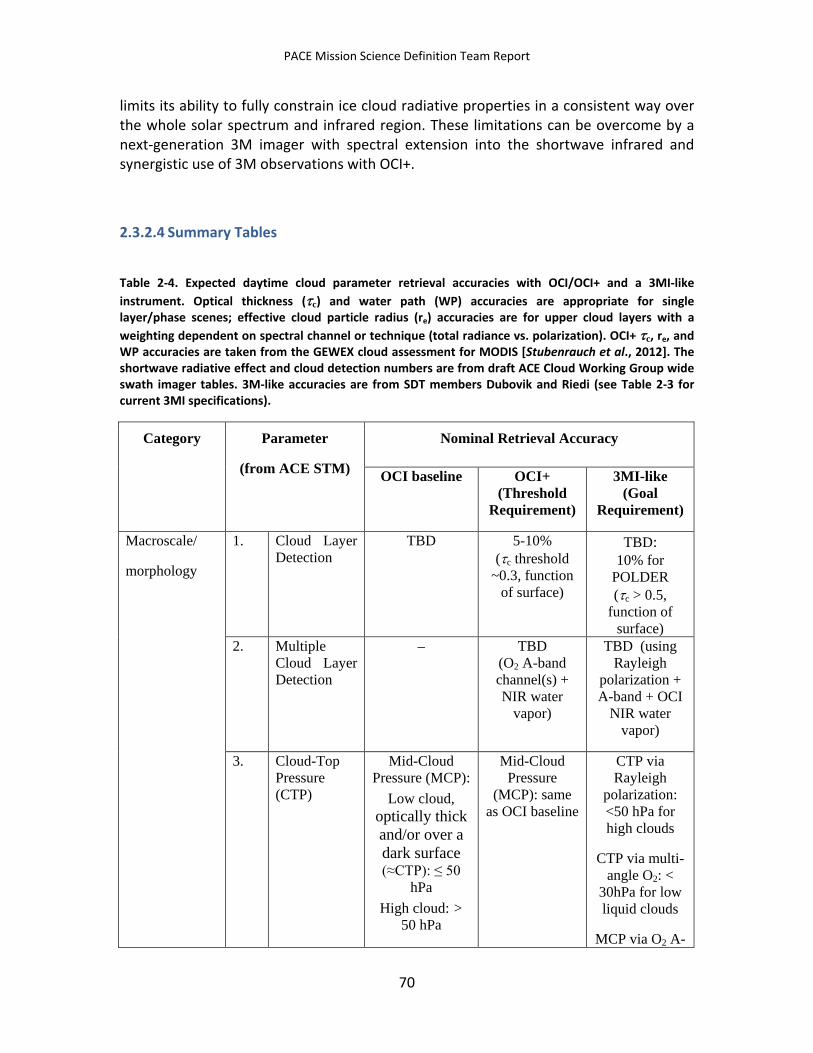
PACE Mission Science Definition Team Report
limits its ability to fully constrain ice cloud radiative properties in a consistent way over the whole solar spectrum and infrared region. These limitations can be overcome by a next-generation 3M imager with spectral extension into the shortwave infrared and synergistic use of 3M observations with OCI+.
2.3.2.4 Summary Tables
Table 2-4. Expected daytime cloud parameter retrieval accuracies with OCI/OCI+ and a 3MI-like instrument. Optical thickness (τc) and water path (WP) accuracies are appropriate for single layer/phase scenes; effective cloud particle radius (re) accuracies are for upper cloud layers with a weighting dependent on spectral channel or technique (total radiance vs. polarization). OCI+ τc, re, and WP accuracies are taken from the GEWEX cloud assessment for MODIS [Stubenrauch et al., 2012]. The shortwave radiative effect and cloud detection numbers are from draft ACE Cloud Working Group wide swath imager tables. 3M-like accuracies are from SDT members Dubovik and Riedi (see Table 2-3 for current 3MI specifications).
Category Parameter
(from ACE STM)
Nominal Retrieval Accuracy
OCI baseline OCI+ (Threshold
Requirement)
3MI-like (Goal
Requirement)
Macroscale/
morphology
1. Cloud Layer Detection
TBD 5-10% (τc threshold
~0.3, function of surface)
TBD: 10% for
POLDER (τc > 0.5,
function of surface)
2. Multiple Cloud Layer Detection
– TBD (O2 A-band channel(s) + NIR water
vapor)
TBD (using Rayleigh
polarization + A-band + OCI
NIR water vapor)
3. Cloud-Top Pressure (CTP)
Mid-Cloud Pressure (MCP):
Low cloud, optically thick and/or over a dark surface (≈CTP): ≤ 50
hPa High cloud: >
50 hPa
Mid-Cloud Pressure
(MCP): same as OCI baseline
CTP via Rayleigh
polarization: <50 hPa for high clouds
CTP via multi-angle O2: <
30hPa for low liquid clouds
MCP via O2 A-
70
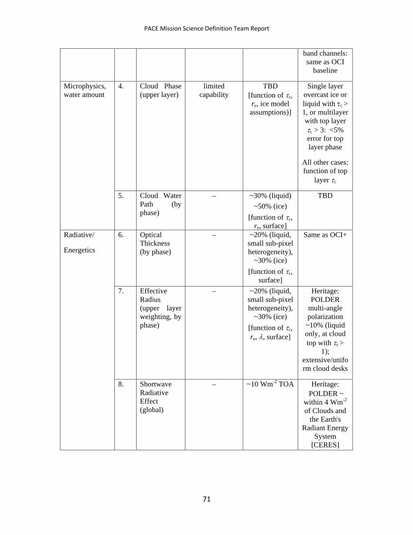
PACE Mission Science Definition Team Report
band channels: same as OCI
baseline
Microphysics, water amount
4. Cloud Phase (upper layer)
limited capability
TBD [function of τc, re, ice model
assumptions)]
Single layer overcast ice or liquid with τc > 1, or multilayer with top layer τc > 3: <5% error for top layer phase
All other cases: function of top
layer τc
5. Cloud Water Path (by phase)
– ~30% (liquid) ~50% (ice)
[function of τc, re, surface]
TBD
Radiative/
Energetics
6. Optical Thickness (by phase)
– ~20% (liquid, small sub-pixel heterogeneity),
~30% (ice) [function of τc,
surface]
Same as OCI+
7. Effective Radius (upper layer weighting, by phase)
– ~20% (liquid, small sub-pixel heterogeneity),
~30% (ice) [function of τc, re, λ, surface]
Heritage: POLDER
multi-angle polarization
~10% (liquid only, at cloud top with τc >
1); extensive/uniform cloud desks
8. Shortwave Radiative Effect (global)
– ~10 Wm-2 TOA Heritage: POLDER ~
within 4 Wm-2 of Clouds and
the Earth's Radiant Energy
System [CERES]
71
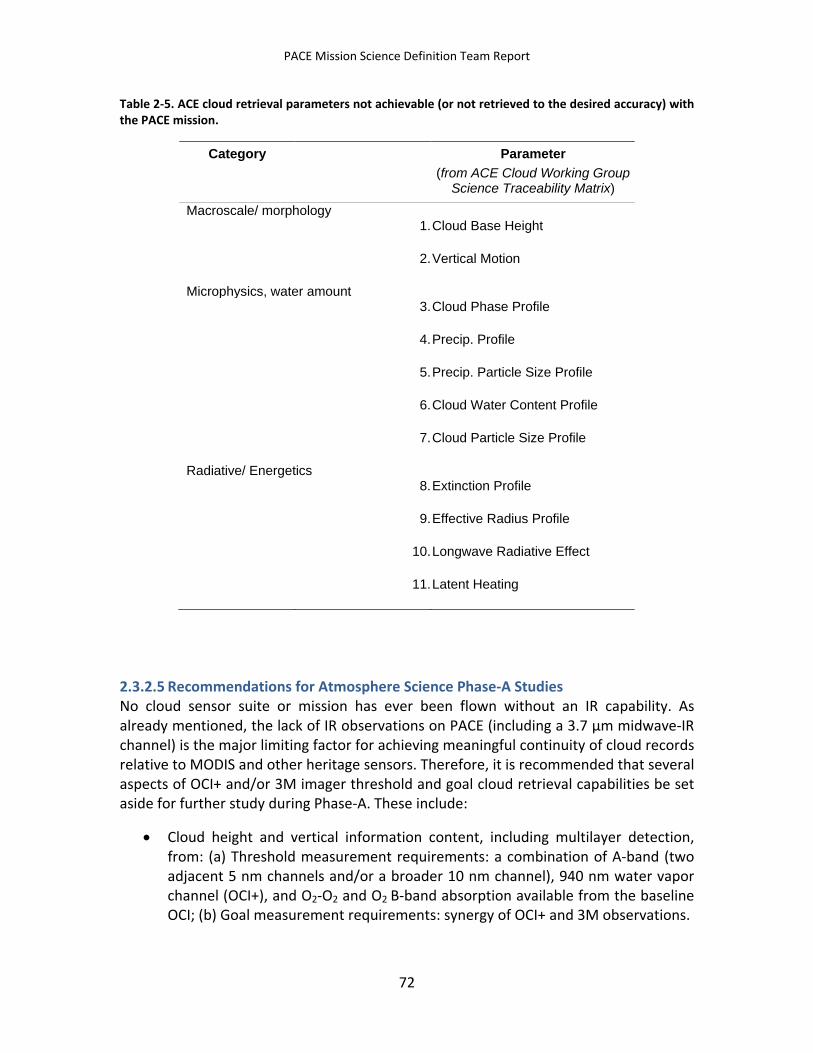
PACE Mission Science Definition Team Report
Table 2-5. ACE cloud retrieval parameters not achievable (or not retrieved to the desired accuracy) with the PACE mission.
Category Parameter (from ACE Cloud Working Group
Science Traceability Matrix)
Macroscale/ morphology 1. Cloud Base Height
2. Vertical Motion
Microphysics, water amount 3. Cloud Phase Profile
4. Precip. Profile
5. Precip. Particle Size Profile
6. Cloud Water Content Profile
7. Cloud Particle Size Profile
Radiative/ Energetics 8. Extinction Profile
9. Effective Radius Profile
10. Longwave Radiative Effect
11. Latent Heating
2.3.2.5 Recommendations for Atmosphere Science Phase-A Studies No cloud sensor suite or mission has ever been flown without an IR capability. As already mentioned, the lack of IR observations on PACE (including a 3.7 µm midwave-IR channel) is the major limiting factor for achieving meaningful continuity of cloud records relative to MODIS and other heritage sensors. Therefore, it is recommended that several aspects of OCI+ and/or 3M imager threshold and goal cloud retrieval capabilities be set aside for further study during Phase-A. These include:
• Cloud height and vertical information content, including multilayer detection, from: (a) Threshold measurement requirements: a combination of A-band (two adjacent 5 nm channels and/or a broader 10 nm channel), 940 nm water vapor channel (OCI+), and O2-O2 and O2 B-band absorption available from the baseline OCI; (b) Goal measurement requirements: synergy of OCI+ and 3M observations.
72
PACE Mission Science Definition Team Report
• Phase information content available from: (a) Threshold measurement requirements: combination of OCI+ SWIR channels (1.62, 2.13, and 2.25 µm); (b) Goal measurement requirements: synergy of OCI+ and 3M observations.
• Daytime studies using MODIS and/or VIIRS cloud mask algorithms, with and without application of IR detection tests, to quantify the reduction in cloud detection skill as a function of cloud height and surface for the OCI/OCI+ channel selection.
• Low cloud spatial resolution studies of retrieval biases in optical thickness and effective radius (specifically, 1.6 and 2.1 µm retrievals relative to a 3.7 µm band) as a function of spatial resolution (<1 km) using theoretical models with explicit microphysics (e.g., Large eddy simulation [LES]), high spatial resolution aircraft imager data, and/or 500 m MODIS data.
Recommended goal aerosol and cloud retrieval capabilities for further study during Phase-A:
• Evaluate the synergistic performance of OCI+ and an advanced 3M imager compared to OCI+ and POLDER. In particular, determine the advanced 3M measurements requirements relative to POLDER (spectral, angular, polarimetric) needed to advance the full range of PACE science questions (see section 2.3.2, as well as ocean color atmospheric correction text).
73

PACE Mission Science Definition Team Report
2.4 Terrestrial Ecology Global land use and climate variability alter ecosystem characteristics, including vegetation structure, function, and biological diversity. Observing these changes requires repeated satellite observations of spectral reflectance. Vegetation spectral reflectance is determined by several factors, including: the amount and type of canopy materials such as leaves and branches (usually expressed by leaf area index [LAI]), the distribution of those canopy materials in space (e.g., crown shape and canopy coverage), and the optical properties of the materials (the spectral reflectance and transmittance of the leaves and branches) [Huemmrich and Goward, 1997; Huemmrich, 2001]. These characteristics are, in turn, shaped by growth forms defined by species and/or functional types, along with the characteristic responses of the species/functional types to environmental conditions due to site differences (e.g., nutrient and soil moisture status), seasonal changes, responses to transient events such as droughts, effects of disturbances such as insect outbreaks, storm damage, fires, logging, and recovery from those disturbances (site history). PACE, by providing frequent global moderate-resolution observations with numerous spectral bands, will provide new global terrestrial ecosystem products that will be directed at a number of important science questions (see below). These capabilities meet requirements of the NRC Decadal Survey [NRC, 2007], which identifies the following terrestrial ecosystem properties as key measurements:
• Distribution and changes in key species and functional groups of organisms
• Disturbance patterns
• Vegetation stress
• Vegetation nutrient status
• Primary productivity
• Vegetation cover
PACE will advance the detection and measurement of all of these properties. Also, in the Science Plan for NASA’s Science Mission Directorate (2007-2016) the Carbon Cycle and Ecosystems focus area calls to “Quantify global land cover change and terrestrial and marine productivity, and improve carbon cycle and ecosystem models.” PACE will provide data that relate high spectral and temporal resolution measurements to ecosystem carbon, energy and water fluxes, including gross ecosystem production (GEP) and evapotranspiration, leading to the development of improved models of terrestrial ecosystem processes.
Current satellite measurements of terrestrial vegetation are generally limited to general land cover, some types of disturbances, vegetation leaf area index, and canopy energy absorption. Existing and expected satellite systems do not provide the combination of
74
PACE Mission Science Definition Team Report
high-resolution narrow-band observations and the high-repeat imaging frequency required to study the fundamental causes of vegetation physiological dynamics. MODIS and VIIRS provide frequent observations, but in broad spectral bands. Hyperion and future missions such as EnMap and HyspIRI provide narrow-band hyperspectral data, but these data are collected infrequently. Aircraft mounted instruments such as Airborne Visible/Infrared Imaging Spectrometer (AVIRIS) and Compact Airborne Spectrographic Imager (CASI) can provide data with high spectral and spatial resolution, however they are only available for small areas and are rarely flown with the frequency and duration to observe daily to seasonal vegetation dynamics.
2.4.1 Top-order Goal Terrestrial Ecology Science Questions
2.4.1.1 Terrestrial Ecosystem Biophysical and Biochemical Characteristics Vegetation biophysical and biochemical characteristics define ecosystem productivity and reflect responses to environmental conditions. Subtle patterns of vegetation activity reflect underlying physiological dynamics and require hyperspectral capabilities with frequent repeated observations to be discerned. Improved assessment of vegetation pigment levels can infer plant physiological status, improving inputs to models of carbon exchange, and identify periods of stress and reduced photosynthetic activity.
Current approaches to describing terrestrial gross ecosystem production (GEP) use modeled parameters to include expected reductions in carbon uptake due to environmental stresses. Jung et al. [2007] found that changing the meteorological drivers in terrestrial ecosystem models results in substantial differences in estimates of GEP, and, in particular, uncertainties in estimating the light use efficiency (LUE) were a key difference between models. In an effort to quantify errors in modeled carbon fluxes and their sources Lin et al. [2011] determined that the largest cumulative errors come from parameters controlling the LUE. Martel et al. [2005] found that the MODIS-Land GEP product estimates in late season were about twice as high as in situ eddy covariance measurements. Although the estimates of air temperature used in the GEP model closely tracked the ground data, the maximum LUE parameter, determined partly from air temperature, in the MODIS algorithm was much higher than that indicated by the tower measurements [Martel et al., 2005].
Vegetation structure controls light interception, so changes in LAI, along with the fraction of photosynthetically active radiation absorbed by plants (fPAR) through the growing season, are key parameters in ecosystem models. While multispectral approaches exist to derive these variables, improvements in their estimation can be achieved with hyperspectral data, such as the minimization of soil background and atmospheric effects [Broge and Leblanc, 2000; Hall et al., 1990] and avoiding saturation of vegetation indices at high LAI values [Haboudane et al., 2004].
Beyond the structural characteristics of vegetation canopies, determining plant
75
PACE Mission Science Definition Team Report
pigments is key to understanding vegetation physiological status. Pigment concentrations play an important role in plant photosynthesis and protection. There are three major classes of plant pigments: chlorophylls, carotenoids, and anthocyanins [Blackburn, 2007; Gitelson, 2011]. Chlorophyll concentrations control potential photosynthesis and provide an indirect estimate of plant nutrient status [Filella et al., 1995; Moran et al., 2000]. The ratio of chlorophyll-a to chlorophyll-b changes with environmental factors, such as light levels [Fang et al., 1998], providing a descriptor of plant-environment interactions [Richardson et al., 2002]. In plants, carotenoids have both photosynthetic and photoprotective functions. Carotenoids are structural components of the photosynthetic antenna and reaction center complexes [Bartley and Scolnik, 1995]. Further, xanthophyll pigments are types of carotenoids that are important in photoprotection (see below). Anthocyanins play a variety of roles in plants and are a common pigment in all leaves. For certain species or growth stages anthocyanins may even become the dominant type of pigment. They can alter the light environment within a leaf and thus regulate photosynthesis and limit photoinhibition and photobleaching [Barker et al., 1997; Steyn et al., 2002; Close and Beadle, 2003]. Beyond photoprotection, anthocyanins may provide some protection from freezing and drought stress [Chalker-Scott, 1999], as well as aid recovery after injury [Gould et al., 2002].
In circumstances when the leaf absorption of photosynthetically active radiation (PAR) exceeds the capacity of the photosynthetic processes to use that energy, reactions in the xanthophyll cycle cause the pigment violaxanthin to reverse epoxidation to form zeaxanthin via antheraxanthin. This process releases energy as heat and is reversible when PAR levels are reduced [Grace et al., 2007; Coops et al., 2010]. The spectral properties of these pigments cause an observable change in leaf reflectance at 531 nm [Gamon et al., 1992; Peñuelas et al., 1995; Middleton et al., 2011]. Photochemical Reflectance Indices (PRI) are spectral indices designed to detect this reaction, although the PRI signal also comes from carotenoid/chlorophyll ratios and conformational changes in chloroplasts [Filella et al., 2009]. PRI is a normalized difference ratio of two narrow visible wavelengths (typically 531 nm—the detection band, and a reference band, often at 570 nm). A number of field and remote sensing studies have demonstrated that PRI is strongly related to foliage or ecosystem LUE [Gamon and Qiu, 1999; Nichol et al., 2000; Rahman et al., 2001, 2004; Raddi et al., 2001; Grace et al., 2007; Hilker et al., 2008; Garbulsky et al., 2008, 2011; Peñuelas et al., 2011]. PRI has been successfully calculated from MODIS data by using the ocean bands over land. MODIS band 11 centered at 531 nm is the detection band, however, a 570 nm band is not available on MODIS so for a reference band one of the MODIS bands such as those centered at either 488, 551, 645 or 678 nm (bands 10, 12, 1, and 13, respectively) have been used [Rahman et al., 2004; Drolet et al., 2005, 2008; Goerner et al., 2010; Huemmrich et al., 2009; Middleton et al., 2011]. MODIS PRI studies cannot be continued using VIIRS as it lacks a 531 nm band.
76
PACE Mission Science Definition Team Report
TSQ-1: What are the structural and biochemical characteristics of plant canopies? How do these characteristics affect carbon, water, and energy fluxes?
2.4.1.2 Terrestrial Ecosystem Dynamics Terrestrial vegetation responds to changing environmental conditions in different ways at different timescales: successional vegetation changes may take decades; structural changes, such as seasonal leaf area index (LAI) variability, occur over days to months; vegetation water content may change over several days; and biochemistry/physiology changes, including chlorophyll content, changes over days, with xanthophyll cycle pigments and fluorescence changing over periods of seconds to hours. The magnitude, rate, and duration of these responses are related to ecosystem processes such as carbon balance and evapotranspiration. The response rates and magnitudes vary among vegetation types and phenologic stages, and with the nature and intensity of environmental stresses. For example, leaf biochemical changes in the chlorophyll to carotenoid ratio are indicators of stress effects and phenological stage [Young and Britton, 1990] and variability of anthocyanin concentrations provide information on the physiological responses of plants to environmental stresses due to episodic events or seasonal changes. Rapid changes in pigment concentrations can be indicators of stress responses to environmental changes such as drought. Further, early detection of these stress responses may foreshadow serious disturbance events like fires or insect outbreaks. Detection and diagnosis of the causes of ecosystem responses to climate change and other types of disturbances require the ability to observe and monitor high temporal frequency changes in vegetation physiology and structure, as PACE will provide.
TSQ-2: What are the seasonal patterns and shorter-term variations in terrestrial ecosystems, functional groups, and diagnostic species? Are short-term changes in plant biochemistry the early signs of vegetation stress and do they provide an indication of an increased probability of serious disturbances?
2.4.1.3 Terrestrial Ecosystem Pattern and Spatial Distribution The distribution of terrestrial ecosystems across the Earth is largely controlled by climate, modified by substrate and other factors. Human modifications further alter ecosystems. Variations in the response of different types of vegetation to environmental changes (both human and naturally induced) provide a more advanced method of vegetation mapping by creating “functional maps” of spatial patterns of carbon and water exchange. Suites of plant species can be organized into assemblages possessing similar forms and functions, referred to as plant functional types (PFTs). PFTs may be discriminated by structure and foliage pigment concentrations with unique seasonal changes and stress responses in biochemistry and structure offering additional leverage for discriminating PFTs. Due to the importance of plant pigments, descriptions of
77
PACE Mission Science Definition Team Report
temporal and spatial variations in pigments provide key information for a wide range of terrestrial ecosystem studies and applications. Improved descriptions of PFTs and their distributions will significantly improve models of ecosystem processes. PACE provides data that supports these studies.
TSQ-3: What are the global spatial patterns of ecosystem and biodiversity distributions, and how do ecosystems differ in their composition? Can differences in the response of optical signals to environmental changes improve the ability to map species, characterize species diversity, and detect occurrence of invasive species?
2.4.2 Advancing Terrestrial Science with PACE PACE provides a strong synergy with HyspIRI. HyspIRI will make hyperspectral observations with approximately 10 nm bands over a spectral range of 400 to 2500 nm, every 19 days at 60 m. It will provide high spatial resolution views of terrestrial landscapes, occasionally to match up with PACE’s frequent low spatial resolution views. HyspIRI will also provide 1 km hyperspectral data over oceans.
PACE can simulate the MODIS land bands, so provides continuity with MODIS products. Some MODIS products, such as vegetation continuous fields and visible albedo, can be improved by taking advantage of the multiple visible bands of PACE. Further, PACE is required to continue MODIS PRI as VIIRS does not have the required 531 nm band.
2.4.3 Issues and Solutions There are a number of different approaches for determining foliage pigment contents from optical signals. These approaches can be generally grouped as: vegetation indices [e.g., Hilker et al., 2011; Gitelson, 2011], spectral derivatives and continuum removal [e.g., Zarco-Tejada et al., 2003, 2004], and model inversions [e.g., Hilker et al., 2011; Zhang et al., 2009, 2011]. All of these approaches require multiple narrow spectral bands [Blackburn, 2007]. Presently, foliage pigment concentrations are not produced as data products from MODIS or VIIRS.
78
PACE Mission Science Definition Team Report
2.5 Watersheds and Lakes
2.5.1 Importance of Lakes and Watersheds to the Carbon Cycle and the Exchange of Biogeochemical Elements between Land and Sea
Inland fresh water bodies are key to the economic and social vitality of growing urban and rural human communities around the planet for food production, transportation, tourism, and water supply. The total area of freshwater lakes, ponds, and impoundments on Earth sums to ~4.2 million km2 and this area is dominated by water bodies smaller than 1 km2 [Downing et al., 2006]. Until the end of the 20th century, the integrated area of lakes was estimated to be only 1.3-1.8% of the land surface [Meybeck, 1995; Schuiling, 1977; Wetzel, 1990]. However, better statistical methods combined with improved models suggest that >3% of the total land area on Earth is occupied by inland water ecosystems. An additional two percent of the land area is covered by marshlands and swamps [Downing et al., 2006; Groombridge and Jenkins, 1998].
Lakes fundamentally act as catchments for precipitation, much of which has percolated through complex soil types. Rivers are complicated bodies of water, which drain land by gravity towards the sea. Lakes and rivers represent critical habitat for both freshwater fish and fish that live part of their lives in salt water and part in freshwater (diadromous fish). From these environs, fresh waters flow downstream through sequential watersheds, collecting new dissolved and particulate materials. Rivers and lakes also accumulate anthropogenic materials (nutrients from fertilizers, urban runoff, pollutants) during their transit to the sea. Ultimately, these fresh waters mix with ocean water in estuaries, where critical nursery grounds for fish, invertebrates, and microfauna are located. The co-location of dense human populations along coasts with coastal estuaries makes them some of the most susceptible environments to human impact. Estuaries are among the most productive and diverse habitats in the biosphere [Groombridge and Jenkins, 1998], yet little is known about the aggregate impact of rivers and lakes on global biodiversity and global biogeochemical cycles. It has been difficult to assess their synoptic properties and variability using remote sensing methods due to their complex water types, plus their dynamic variability through time and space. To date, aquatic scientists have lacked the high-quality, frequent and global hyperspectral (or even multi-spectral) remote sensing observations to observe how these freshwater ecosystems are changing.
Within the context of global lakes, ponds, and impoundments, the Great Lakes are of special interest to the United States, particularly given their size and economic importance. According to the U.S. EPA (http://www.epa.gov/glnpo/atlas/index.html), the Great Lakes cover ~244,000 km2—5.8% of the area of all freshwater lakes, ponds and impoundments on Earth. With their total volume of 22,700 km2, they contain 21% of the global supply of freshwater and 84% of the freshwater of the United States. They have some 17,000 km of shoreline, populated by roughly 1/10th of the U.S. population
79
PACE Mission Science Definition Team Report
(and almost 1/3 of the Canadian population). The Great Lakes collect the runoff from 0.5 million km2 of North American lands.
One of the most difficult problems in ocean color remote sensing is the deciphering of optically-complex coastal waters in turbid environments with complex mixtures of particulate and dissolved matter and shallow optical depths. The nature of the problem was first recognized with the differentiation between Case-I waters (where phytoplankton and water represent the major influences on the overall optical properties) versus Case-II waters (in which factors over and above water and phytoplankton significantly impact the optical properties) [Gordon and Morel, 1983]. In the case of the latter, terrestrially-derived sediments and chromophoric dissolved organic matter (CDOM) are major sources of “Case-II particulate” and “Case-II dissolved” materials, respectively. In practice, this discrimination has been done in the coastal ocean (a few kilometers from shore out to the shelf break) where concentrations of these constituents are high enough that the performance of standard ocean color algorithms for chlorophyll degrades.
Assessing Case-II waters using optical methods has become more tractable in recent years [Gitelson et al., 2007; Pozdnyakov et al., 2005; Stumpf, 1987; Stumpf et al., 2003; Stumpf and Pennock, 1989; Witter et al., 2009)]. Regional algorithms show improvements [Darecki and Stramski, 2004]. It is worthy of note that most of the algorithm products for these waters are for retrieving chlorophyll and suspended particulate matter concentrations. However, there are still significant challenges in lakes and watersheds to accurately measure geophysical properties where the turbidity and suspended particulate- and dissolved matter concentrations can be orders of magnitude higher than in typical ocean waters [Dall'Olmo and Gitelson, 2006].
2.5.2 Spatial and Temporal Scales Required to Characterize Lakes and Watersheds
From a remote sensing perspective, satellite studies of lakes and watersheds have been limited by relatively slow sensor-dynamic responses to changing radiance signals. This means that as sensing elements transition from relatively high reflectance targets (like the land) to low-reflectance targets (like water) the radiometric accuracy degrades. The image analysis property known as “land-ringing” is defined as the regions of an image where pixels must be flagged due to the fact that the sensors were transitioning from one radiance extreme to the other, hence the data have questionable accuracy. Typically regions of an image that are flagged for land-ringing are several pixels around the water-land boundary (which means a band of several kilometers is lost). Note that from a management perspective, this is precisely the region of greatest interaction between humans and the aquatic environment, containing dwellings, recreation, fishing, industry, tourism, etc. There are additional problems, including multiple scattering of photons from sunlight reflected off the land, which contribute to the radiance of the
80
PACE Mission Science Definition Team Report
atmosphere adjacent to a coastline. Further, land-derived aerosols tend to dominate the atmosphere over lakes, and aerosol radiance correction algorithms used over the ocean may not be applicable. These issues present problems for the study of lakes and watersheds since most are smaller than this size scale. Since the early days of the Coastal Zone Color Scanner (1970s) and through the SeaWiFS era into the MODIS and VIIRS era, U.S. ocean color remote sensing instruments have focused on the high-quality radiometric observations that are afforded by coarser-resolution sensors with pixels of about one kilometer square. Yet, of the 0.3 billion standing water bodies (lakes, ponds and impoundments) spread over the Earth, >90% are one hectare (100 m x 100 m) in area or smaller [Downing et al., 2006]. To address this problem, and facilitate routine and repeated scientific observation to address climate signals, pixel size must be reduced, while sensor dynamic response within the imaging elements must be quickened. The requirements include maintaining high radiometric quality while reducing instrument artifacts.
Improvements in the remote sensing of inland waters have already been demonstrated using sensors such as the Hyperspectral Imager for the Coastal Ocean (HICO) operating on the International Space Station. This instrument is the first space-based hyperspectral instrument developed primarily for imaging of lakes, rivers, estuaries and coastal waters.
Rivers also play an important role in the Earth’s hydrology, as they represent a significant area of freshwater within the terrestrial system. They also suffer from the same problems discussed above. In terms of their size, the average river widths vary between wet and dry seasons, but widths of some of the more significant rivers are: Mississippi (dry season) = 1.6 km, St Lawrence = 3.3 km, Nile = 8 km , MacKenzie (largest river emptying into the Arctic and in top 20 rivers globally) = 0.3-6 km, Congo River = 0.8-16 km, and Amazon (largest river catchment on Earth, 6.1 million km2 catchment area) = 1-10 km (dry to wet season). Given these widths and lake sizes, an ability to derive sub-kilometer resolution aboard PACE would allow improved resolution of the river-born, land-to-sea carbon fluxes, for more than just the biggest rivers.
The time scales that are of interest for following biogeochemical variability within lakes, rivers, and watersheds (hence relevance to a polar orbiting satellite platform such as PACE) are typically one day or longer. Seasonal variability, through dry and wet seasons, is a first-order factor affecting watershed biology, chemistry and geology. Annual, decadal and century time scales are also all relevant to understanding climate change and its impacts on land-to-sea carbon acquisition and export, and on the productivity and biodiversity that we depend on for food, water, and other ecosystem services.
2.5.3 Characterizing Water Types in Inland Waters Table 2-6 shows geophysical parameters that need to be observed from space to characterize inland to oceanic waters. Specifically, the table provides the upper limits of
81
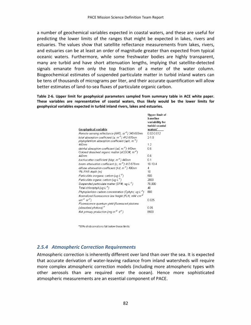
PACE Mission Science Definition Team Report
a number of geochemical variables expected in coastal waters, and these are useful for predicting the lower limits of the ranges that might be expected in lakes, rivers and estuaries. The values show that satellite reflectance measurements from lakes, rivers, and estuaries can be at least an order of magnitude greater than expected from typical oceanic waters. Furthermore, while some freshwater bodies are highly transparent, many are turbid and have short attenuation lengths, implying that satellite-detected signals emanate from only the top fraction of a meter of the water column. Biogeochemical estimates of suspended particulate matter in turbid inland waters can be tens of thousands of micrograms per liter, and their accurate quantification will allow better estimates of land-to-sea fluxes of particulate organic carbon.
Table 2-6. Upper limit for geophysical parameters sampled from summary table in ACE white paper. These variables are representative of coastal waters, thus likely would be the lower limits for geophysical variables expected in turbid inland rivers, lakes and estuaries.
2.5.4 Atmospheric Correction Requirements Atmospheric correction is inherently different over land than over the sea. It is expected that accurate derivation of water-leaving radiance from inland watersheds will require more complex atmospheric correction models (including more atmospheric types with other aerosols than are required over the ocean). Hence more sophisticated atmospheric measurements are an essential component of PACE.
82
PACE Mission Science Definition Team Report
2.5.5 Relevance to NASA Goals in Climate Science By providing capabilities on PACE to remotely sense lakes, rivers, and estuaries, the mission will better support the national needs outlined in the recent NASA report, “Responding to the Challenge of Climate and Environmental Change: NASA’s Plan for a Climate-Centric Architecture for Earth Observations and Applications from Space” [NASA, 2010]. Principally, the critical needs are (1) climate monitoring and research, and (2) carbon cycle research. The latter goal implicitly assumes accurate understanding of carbon storage in and exchange among the atmosphere, ocean and biosphere as critical to projecting with confidence the future evolution of climate. Global measurements of the color of the hydrosphere from space complement data from in situ and surface measurement networks, and will be critical for understanding the fundamental issues associated with Earth’s climate change. Along with the above global climate relevance, the remote sensing of aquatic water bodies can offer significant advances for assessing lake and river health, plus critical environmental information for proper management of aquatic water bodies. Clearly, the largest United States lakes are highly relevant to economic, environmental, and human health (e.g., Great Lakes, Great Salt Lake, Lake Okeechobee, Lake Pontchartrain, Lake Champlain, etc.). Nonetheless, global stewardship of lakes and water bodies (both national and international) will become increasingly critical as populations grow and water resources diminish. PACE will be well situated to provide such important information.
83
PACE Mission Science Definition Team Report
3 PACE Science-Driven Measurement Requirements
3.1 Introduction This section presents the measurement requirements that are necessary to address science questions related to ocean ecology and biogeochemistry, atmosphere, and terrestrial ecology. Inland waters and watershed measurement requirements overlap those of coastal ocean research, and are addressed together this section. Following our "whole mission concept" approach, this section presents very detailed measurement and mission requirements that include instrument characteristics and measurement and data management strategies, amongst others. These requirements are based on the community’s experience with Earth science missions, and on studies and analyses done by the SDT during the preparation of this report. As explained in the introduction, the SDT was very prescriptive when it considered that a particular technical specification, measurement approach, or mission management practice was the most appropriate or safe to obtain high quality research data. The SDT strongly recommends following these recommendations.
3.2 Ocean Ecology and Biogeochemistry The introductory section on PACE ocean ecology and biogeochemistry identifies seven threshold ocean Science Questions (SQ) and associates each of these questions to a specific set of geophysical properties or processes. These sets of science-driven property retrievals define measurement requirements that exceed those of heritage sensors, particularly in terms of measurement spectral range and resolution. PACE science objectives also extend from near-shore waters to the broad open ocean, which has implications on desired spatial resolution. Multiple aspects of the PACE threshold ocean Science Questions are also several steps removed from the primary observations of the PACE ocean radiometer, and thus require additional inputs from contemporaneous operational satellites, in situ oceanographic and atmospheric observations, and significant integration of PACE data into Earth system models. The ocean ecology and biogeochemistry introduction also describes PACE approaches for achieving ocean science objectives through retrievals of essential ocean ecosystem and biogeochemical properties (subsections 2.2.2.1 through 2.2.2.17), including a mapping of measurement spectral bands to specific retrieved properties.
In this section, a detailed description is provided of science-driven measurement requirements for retrieving key PACE ocean geophysical parameters. In each subsection, we explain the justification for each requirement and identify additional desirables beyond the threshold ocean science requirements that could enhance the scientific benefits of the PACE mission. At the end of each subsection, ocean science threshold requirements and goal capabilities are summarized. We emphasize that attributes designated as goals do not represent a trade-space for achieving threshold
84
PACE Mission Science Definition Team Report
requirements, but instead the additional ‘goal’ requirements represent an advantage only if accomplished in addition to meeting all PACE ocean science threshold requirements. Finally, we reiterate that success of PACE science relies not only on the exceptional satellite measurement capabilities defined herein, but also on a comprehensive mission design that integrates a rigorous calibration/validation program, repeated data reprocessing, and field-based research in support of algorithm development and product validation. These broader mission requirements are discussed in detail in other sections of this SDT report. Measurement requirements are described in the subsections below.
3.2.1 Orbit It is recommended that a near-noon sun-synchronous polar orbit for PACE be chosen because it (1) provides high illumination intensities for accurate retrievals from the relatively dark ocean, (2) minimizes atmospheric path lengths for improved atmospheric corrections, (3) minimizes the range of scattering angles for simplification of atmospheric corrections and surface bidirectional reflectance effects, (4) maximizes repeat observations of high latitudes to improve probabilities of viewing cloud-free scenes each day, and (5) maximizes coverage of the entire Earth in the shortest amount of time. Based on experience with heritage ocean color sensors, a noon equatorial crossing time is optimal for addressing these considerations, although a window of 11:00 to 1:00 could be considered if a non-noon orbit within this wider window provides significant advantage for other science communities served by the PACE ocean radiometer (note, for a morning crossing time, a descending orbit is recommended; for an afternoon crossing time, an ascending orbit is recommended). In addition, it is recommended that the PACE orbit be maintained over the mission lifetime to ±10 minutes to ensure that the heating and cooling cycles of the spacecraft remain constant throughout the mission lifetime, which reduces potential sensor characterization issues.
Threshold Requirement: Sun-synchronous, polar orbit with an equatorial crossing time between 11:00 and 1:00 and orbit maintenance to ±10 minutes over the lifetime of the mission.
Goal: Noon equatorial crossing time.
3.2.2 Spatial and Temporal Coverage The PACE ocean radiometer will provide observational data for applications across a wide range of space and time scales. Within the temporal domain, issues include maximizing successful matchups between field and satellite observations, tracking of bloom dynamics, and achieving clear-scene observations within a given period in a cloud-dominated atmosphere. Based on experience with heritage ocean color sensors, global observations every two days yield an adequate global fraction of clear-sky scenes
85
PACE Mission Science Definition Team Report
to allow global-scale ecological and biogeochemical computations at 8-day resolution. For more regional analyses, two-day global coverage can allow evaluations at 1-4 day resolution (note that two-day global coverage typically means that many regions of the ocean are viewed at least once per day). A polar orbit with two-day global coverage also ensures that multiple views per day are achieved at higher latitudes, thus improving the probability of clear-sky scenes in these particularly cloudy regions. It is therefore recommended that two-day global coverage within a solar zenith angle of 75o is the threshold requirement for PACE. However, 1-day global coverage is viewed as advantageous for improving the temporal resolution of science investigations if contemporary technologies allow this advance without compromising other measurement requirements for PACE. To achieve PACE global coverage requirements, view zenith angles relative to surface normal (i.e., cross-track) should not exceed 60o, as broader angles result in long atmospheric path lengths (increased uncertainty in atmospheric correction) and can be associated with large pixel expansion (depending on instrument design). In addition, an important ‘lesson learned’ from heritage instruments is that avoidance of sun glint is critical for maximizing successful retrieval coverage for a given instrument design and for maximizing matchup observations with field calibration/ validation data. Thus, sun glint avoidance (i.e., mitigation of glint effects) is an integral component of the threshold global coverage requirement for the PACE ocean radiometer. Glint avoidance was achieved with the SeaWiFS sensor using a ±20o tilt mechanism and a similar approach for PACE can be considered a low-risk option, although alternative approaches may be considered if they can achieve equivalent glint avoidance [Gregg and Patt, 1994].
A key ocean science objective for PACE is to create a global observational data set that allows evaluation of relationships between ocean ecological/biogeochemical properties and environmental forcings. To ensure the success of this objective, it will be highly beneficial for the PACE mission to extend across an adequate time frame to capture significant interannual variability. The ENSO cycle is a major natural form of interannual climate variability. A PACE minimum mission duration of 5 years will ensure reasonable likelihood of capturing ENSO minima and maxima. A mission duration of 10 years, on the other hand, would ensure observations over at least one or more full ENSO cycles and would also capture portions of other longer term oscillations. It is the recommendation of the SDT that the PACE mission have a minimum duration of 5 years and a goal of 10 years. However, it is also recognized that the science benefit of this extended lifetime could also be achieved if a PACE mission with a 3-year minimum lifetime and 5-year goal was followed by a second mission with equivalent measurement capabilities, such that the combined data record from the two missions extended over a 5 to 10 year period.
Threshold Requirement: Two-day global coverage to solar zenith angle of 75o, mitigation of sun glint, multiple daily observations at high latitudes, and sensor view zenith angles not exceeding 60o. Mission lifetime of 5 years.
Goal: One-day global coverage throughout as much of the Earth’s oceans as is possible. Coverage to a solar zenith angle >75o. Mission lifetime of 10 years.
86
PACE Mission Science Definition Team Report
3.2.3 Navigation and Registration The primary drivers for the image navigation and band registration requirements are as follows. Accurate data geolocation is required to enable processing in coastal, as well as open ocean, regions. Specifically, the viewed locations must be known to a fraction of a pixel to enable the effects of coastlines on the nearby measurements to be accurately estimated. Thus, threshold requirements defined here are specific to the threshold spatial resolution of 1 km2, and more stringent requirements would be required for higher spatial resolution ocean data. Accurate geolocation is also required to support match-ups with in situ and ground calibration measurements. Since these measurements are point source observations taken at the surface, sub-pixel accuracy of the satellite-based measurements is again needed to ensure accurate match-ups. The overall pointing knowledge requirement encompasses contributions from all sources, including spacecraft attitude determination, sensor alignment, and sensor viewing geometry, and includes static, dynamic, and random terms. The spatial and temporal consistency of measurements is required across all bands to support retrieval algorithms. Since both the atmospheric correction and water property retrieval algorithms utilize measurements from multiple bands, it is important that all measurements are co-registered (i.e., proximate in both space and time) to reduce the effects of parameter and viewing variations on the algorithms. The stability requirement for sensor pointing is necessary to maintain image coherency (e.g., scan-to-scan for scanning sensors) for users of swath-based images, and also to support instrumental corrections requiring extended measurement fields, such as for stray light. Finally, although the primary requirements are based on ocean measurements, the potential uses of PACE data by non-ocean (e.g., land) communities support stringent goals in this area.
Threshold Requirement: For ocean retrievals at the threshold spatial resolution of 1 km2, the PACE requirement is (1) a pointing accuracy equivalent to 2 Instantaneous Field of View (IFOV) for the specified altitude, and knowledge equivalent to 0.1 IFOV, over the full range of viewing geometries (e.g., scan and tilt angles), (2) a pointing jitter equivalent to 0.01 IFOV between adjacent scans or image rows, (3) a spatial band-to-band registration of 80% of one IFOV between any two bands, without resampling, and (4) simultaneity of 0.02 second.
Goal: Pointing knowledge of 0.05 IFOV. Band-to-band registration of 90% of one IFOV. Simultaneity of 0.01 second.
3.2.4 Instrument Performance Tracking A key component of multiple PACE ocean science questions is the detection of temporal changes in ocean ecological and biogeochemical properties and processes. Many of
87
PACE Mission Science Definition Team Report
these phenomena exhibit strong variability on diel to seasonal time scales. However, a fundamental motivation for the PACE mission is its contribution to the ocean climate data record and advancement of understanding regarding climate-ecosystem relationships. Importantly, the magnitude of interannual changes, or ‘anomalies,’ in ocean ecosystem properties is often much smaller than their shorter time-scale variability. Consequently, characterizing interannual anomalies demands an accurate knowledge of temporal changes in instrument performance. Thus, a requirement for PACE is that degradation/drift in instrument performance be tracked at minimum on a monthly basis through observations of the moon, which represents a stable external source that has been used successfully during the SeaWiFS mission. These observations will be made through the instrument Earth-viewing port and using the same optical path as employed for ocean observations, as this approach minimizes uncertainties in performance characterization associated with changes in components that are not involved in the geophysical retrievals. Relative changes in instrument radiometric performance should be characterized on-orbit for primary science measurement bands to a threshold requirement of ±0.2% and goal of ±0.1% within the first 3 years of the mission and maintained thereafter at this accuracy or better for the duration of the mission. Based on experience with heritage ocean color sensors, this threshold requirement has been achieved by SeaWiFS through monthly lunar observations at a constant phase angle, where all detectors are illuminated during each lunar maneuver. An equivalent approach is recommended for the PACE ocean radiometer for performance tracking (see section 4.4 for additional details). Experience with heritage sensors indicates that tracking of performance changes in instruments with large detector arrays has been challenging because (1) only a fraction of the detectors are illuminated during a given lunar maneuver (e.g., Ocean Color Monitor-2 [OCM-2]), and (2) characterization using solar measurements has the added uncertainty of solar diffuser degradation trending (e.g., MERIS). It should also be noted that instruments like MODIS suffer from a scan-angle-dependent degradation, which adds complexity to the calibration process because the calibration sources (moon and solar diffuser) are only available at selected scan angles (i.e., the degradation measurements must be extrapolated to the remaining scan angles, which—particularly for blue wavelengths—has led to a significant decrease in calibration accuracy. It is essential that these experiences with heritage sensors be carefully considered when evaluating whether a given approach for PACE measurements will enable success in the mission’s key objective of achieving sustained, climate-quality global ocean products.
With respect to instrument calibration, the SDT recommends as a threshold requirement an absolute radiometric calibration to 2% or better prelaunch, and to 5% or better on-orbit (before vicarious calibration). This on-orbit requirement can be achieved through a variety of approaches (e.g., MODIS and VIIRS solar diffuser calibration provides an accuracy to about 2%). The on-orbit threshold of 5% is based on an analysis by Wang and Gordon [2002], where it was shown that the vicarious calibration approach is reliant on knowledge of radiance at a NIR band to an accuracy of 5% (in
88
PACE Mission Science Definition Team Report
other words, this band, which in Wang and Gordon [2002] was centered at 865 nm, is not vicariously calibrated).
An additional requirement for instrument performance tracking is daily measurements of a calibration target to allow detection of sub-monthly changes in instrument performance. For SeaWiFS, instrument performance changes were a remarkably smooth function of time, and were adequately characterized by monthly lunar observations. However, the radiometric degradation of an ocean color sensor does not have to be as graceful (cf., the performance of the MODIS sensor on the Terra platform showed many rapid changes on time scales of less than a month). Hence, daily measurements of a calibration target and dark currents are recommended for PACE to ensure that any unforeseen step-changes in performance can be identified and accounted for (see section 4.4 for additional details). It is recommended that the additional calibration measurements be conducted by viewing an external source (e.g., solar views using diffusers, as with heritage sensors). Temporal degradation of this daily calibration source should be known to ~0.2% between lunar observations. Finally, the PACE requirement for high spectral resolution measurements results in a threshold requirement for a capability to characterize instrument spectral drift over the mission lifetime. A variety of specific approaches may be considered for achieving this requirement, but spectral drift should be detectable and correctable to a minimum accuracy of 0.3 nm.
Threshold Requirement: Monthly characterization of change in all instrument detectors and Earth-viewing optical components using lunar observations through the Earth viewing port. Characterization of instrument radiometric performance changes to ±0.2% within the first 3 years of the mission and maintenance of this accuracy thereafter for the duration of the mission. Prelaunch absolute calibration of 2% and on-orbit absolute calibration accuracy (before vicarious calibration) of better than 5%. Monthly characterization of instrument spectral drift to an accuracy of 0.3 nm. Daily observations of a calibration target/source (e.g., sun) and dark current for high temporal resolution tracking. Characterization of daily calibration target degradation to ~0.2% between lunar observations. Dark current should be measured at every scan.
Goal: Characterization of instrument performance changes to ±0.1% within 3 years and maintenance of this accuracy thereafter on at least a monthly basis.
3.2.5 Instrument Artifacts The PACE mission aims to address current issues in global ocean ecology and biogeochemistry through the climate-quality retrieval of a broad suite of key ocean properties and processes. Success in this endeavor relies on accurate retrievals of spectral normalized water-leaving radiances (nLw). It is desired for PACE that uncertainties in nLw be largely defined by state-of-the-science atmospheric correction errors, with contributions from uncharacterized instrument artifacts kept to an absolute
89
PACE Mission Science Definition Team Report
minimum. These instrument artifacts contribute directly to radiance retrieval uncertainties and thus to errors in derived geophysical parameters. Instrument issues of concern include (but are not limited to) uncharacterized temporal changes in detector performance that give rise to image striping, optical or electronic crosstalk, polarization sensitivity, detector saturation, and scan-angle-dependent responses. Threshold requirements regarding these specific issues are defined below. More broadly, a threshold requirement is that the PACE instrument be thoroughly characterized pre-launch and that a post-launch approach be defined for tracking changes (see section 3.2.4 above). Prelaunch characterization should address all of the instrument properties described in section 3 of Meister et al., 2011, such as dynamic range, linearity, polarization and temperature sensitivity, saturation and recovery, out-of-band responses, stability, and response-versus-scan angle, to name a few. Effective pre- and post-launch characterization is essential for retrieving accurate TOA radiances during Level 0 to Level 1 processing, and is the foundation for achieving climate-quality Level 2 geophysical properties. Uncertainties in nLw associated with uncharacterized instrument artifacts place a greater demand on atmospheric correction accuracies to meet threshold requirements for nLw retrievals (see below). Experience with heritage sensors indicates that instrument artifacts can be reduced to <0.5% of TOA radiances, given an effective approach for characterizing the performance and degradation of all detectors (e.g., SeaWiFS), although this success has not been realized for most heritage instruments. The requirement for PACE is that the total uncertainty uT for a given observation of TOA total radiance be less than 0.5% after vicarious calibration (assuming a perfect vicarious calibration). Let ui be the uncertainty associated with instrument artifact i (where index i indicates, polarization, linearity, stray light, etc.), then uT shall be calculated with
uT = ( ∑I ui2 )1/2
assuming that ui are not correlated.
Image Striping
Uncharacterized differences in the responsivity of multiple detector elements larger than the sensor noise (NedL) within a common spectral band result in an instrument artifact referred to as ‘image striping,’ and susceptibility to this problem is linked to instrument design and ability to uniformly illuminate all detectors during on-orbit calibration maneuvers (see section 3.2.4 above). Raw data from all ocean color sensors have some degree of image striping, but SeaWiFS had very low initial striping (level 0) and was the only sensor that achieved Level 2 products where striping artifacts were characterized and corrected to noise levels. All other heritage ocean color sensors (national and international) have yielded geophysical properties with visible cross-track and/or along-track striping in Level 2 products. For PACE, the recommended threshold requirement is for image striping at <0.1% in calibrated top-of-atmosphere radiances
90
PACE Mission Science Definition Team Report
(i.e., Level 1b products) and derived products that exhibit no image striping (i.e., image striping at noise levels or below).
Optical and Electronic Crosstalk
Crosstalk is defined as an erroneously measured signal for a given measurement wavelength and pixel spatial coordinate that originates from (spatial or spectral) stray light and/or the interaction of electromagnetic fields between neighboring circuits. Crosstalk effects are very difficult and time consuming to quantify and require complicated algorithms to correct. Optical and electronic crosstalk issues have been a particular concern for VIIRS because of problems with optical filter strips and the compactness of the focal plane electronics, but issues were also experienced with SeaWiFS and MODIS. The recommended threshold requirement for crosstalk contributions to radiance uncertainties for PACE is 0.1% at the global typical TOA radiance (Ltyp).
Stray light and bright target recovery
Due to the high contrast between dark ocean and bright clouds (or land areas), stray light and recovery time from measuring a bright target are important aspects of the sensor design. Clouds cover a significant part of the ocean. The area they are covering is obviously not available for ocean color retrievals. But even the area around clouds is a significant part of the global data set. About half of the ocean pixels fall within the MODIS Aqua stray light mask (5x7 pixels), which reduces the data available for Level 3 (L3) processing significantly [Meister and McClain, 2010]. The recommended threshold requirement for stray light contamination for the instrument is less than 0.2% of Ltyp, three pixels away from a cloud (note this threshold of 0.2% is chosen so total uncertainty in TOA radiance does not exceed 0.5% in all areas further than two pixels from a cloud – see section 3.2.5 of Meister et al., 2011). Most heritage ocean color sensors do not meet this requirement, so it is sufficient if this accuracy is reached after application of a stray light correction algorithm. A stray light correction approach [Yeh et al., 1997] has been successfully used for SeaWiFS. However, because the stray light contamination in SeaWiFS is relatively large, even the corrected results do not meet the above requirement for PACE [Barnes et al., 1995]. Clearly, the PACE requirement necessitates a highly accurate pre-launch stray light characterization of the instrument. For details regarding the verification of this issue see Meister et al., 2011, section 3.1.8. Note that cloud radiances used to establish the above threshold requirement never exceed 50 x Ltyp due to the extreme brightness of clouds relative to Ltyp in the NIR and SWIR wavelengths. The recovery effects when measuring a bright light source are included in the specification defined here.
91
PACE Mission Science Definition Team Report
Out of band response
The relative spectral response (RSR) of a band describes the response of the band to monochromatic light. The RSR is normalized to 1.0 at its maximum value. The RSRs of all bands (multispectral and hyperspectral) must be measured pre-launch for all wavelengths. The in-band response is defined as that wavelength region where the RSR is greater than 0.01, the out-of-band response is where the RSR is smaller than 0.01. The integral of the RSR over the out-of-band region divided by the integral of the RSR over the in-band region shall be less than 0.01 for all multispectral channels in Table 3-1. See Meister et al., 2011, sections 3.2.1 and 3.2.2 for further details regarding the RSR characterization.
Polarization Sensitivity
The response of an ocean color instrument to completely linearly polarized light is expected to vary as a function of the polarization phase angle (which describes the axis of vibration of the electric field vector, [Meister et al., 2005]). Gordon et al. [1997] indicate that a 2% polarization sensitivity can lead to errors in the atmospheric correction that increase the uncertainty of the resulting nLw at 443 nm by up to 10%. Given this sensitivity, the recommended upper limit for polarization sensitivity of the PACE ocean sensor is 1%. The SeaWiFS design minimized inherent polarization sensitivity by limiting the angle of incidence range for light on its half-angle mirror (HAM), whereas the MODIS rotating mirror had a much larger range, and the area of reflection off the mirror into the aft optics varied across the mirror during the scan (which is why the mirror had to be so large) [Meister et al., 2011]. SeaWiFS also employed a depolarizer. While the upper limit for polarization sensitivity of the PACE ocean sensor is stated above as 1%, it is further recommended as a threshold requirement that this polarization sensitivity is known (i.e., characterized) to an accuracy of within 0.2% (most of the TOA radiances have a degree of linear polarization of less than 50%). This characterization to 0.2% allows correction for sensor polarization sensitivity properties and permits uncertainty in TOA radiances due to polarization to be less than 0.1% for a large majority of global ocean cases [Meister et al., 2011]. This polarization requirement for PACE is consistent with recommendations from the ACE science team [see appendix of ACE Ocean Biology White paper, 2010)].
Detector Saturation
Detector saturation is a potential issue for ocean color remote sensing because the signal from clouds and the atmosphere is very high compared to that from the ocean. When saturation occurs, it becomes extremely difficult to correct sensor data for stray light and, for instruments employing Charge-Coupled Device (CCD) arrays, saturation results in blooming of electrons in the detector spatial and spectral dimension.
92
PACE Mission Science Definition Team Report
Furthermore, a finite detector recovery time is required following saturation (hysteresis), during which ocean color retrievals are invalid. Finally, the PACE ocean radiometer is intended to serve the scientific objectives of both the oceanographic and atmospheric communities. Thus, accurate radiance retrievals are required during bright scenes (i.e., clouds, aerosols) for many PACE measurement bands, which cannot be achieved with saturated detectors. Taken together, these considerations lead to the recommended threshold requirement for PACE that no saturation should occur for any science measurement bands at Lmax. Given this threshold requirement, it should also be noted that for a small number of instances, TOA radiances can exceed Lmax by up to 1.2 × Lmax [Meister et al., 2011]. It may therefore be viewed as beneficial if saturation is still avoided by the selected PACE instrument on these rare occasions.
Linearity
In most sensors, the relation between radiance and measured counts (dn) is not a perfectly linear function of dn. It is required that this relation be characterized pre-launch with an uncertainty of 0.1% (or 0.0005*Ltyp, whichever is larger) over the whole dynamic range. Note that it is important to characterize linearity even below the expected on-orbit radiances because many pre-launch characterization measurements (e.g., spectral response, stray light) will be at very low light levels. Since there are no available techniques to monitor linearity on-orbit with an accuracy of 0.1%, the design of the instrument shall lead to the expectation that the linearity will not change on-orbit.
Response versus View Angle
In scanning ocean color sensors, significant variations in photon collection efficiency can occur as a function of scan angle. This ‘response versus view angle’ (RVVA) issue was not a significant problem for the SeaWiFS because of its rotating telescope design, but it has been a major issue for the large rotating mirror of MODIS. While a significant RVVA dependence was recognized early on for MODIS and characterized pre-launch, the daunting challenge for MODIS data processing has been that the RVVA has been changing over time, with few on-orbit options for characterizing these variations. The MODIS problem was worsened by mirror-side differences in performance properties. Given the primary objective of the PACE ocean radiometer of achieving a climate quality ocean color data set, it is essential that RVVA artifacts be minimized to the greatest extent possible. It is therefore recommended as a threshold requirement that the response of the PACE radiometer to a constant radiance source varies with view angle by <5% for the entire view angle range (note that the pre-launch RVVA was 2% or less for SeaWiFS, depending on focal plane) and by <0.5% for view angles that differ by less than 1o. The RVVA properties of the PACE radiometer should be characterized pre-launch to an accuracy of 0.1% over the TOA radiance range corresponding to valid ocean
93
PACE Mission Science Definition Team Report
color retrievals (this range is wavelength dependent and, based on SeaWiFS data, is 50 to 125 W [m2 µm sr]-1 at 412 nm and 2.2 to 16 W [m2 µm sr]-1 at 865 nm [Table 3.2 in Meister et al., 2011]).
Threshold Requirement: Thorough prelaunch instrument characterization of linearity, RVVA, polarization sensitivity, radiometric and spectral temperature sensitivity, high contrast resolution, saturation, saturation recovery, crosstalk, radiometric and band-to-band stability, bidirectional reflectance distribution, and relative spectral response [see Meister et al., 2011 for details]. Post-launch approach for tracking performance changes (see section 3.2.4 above). Overall instrument artifact contribution to TOA radiance retrievals of <0.5%. Characterization and correction for image striping that reduces this artifact to noise levels or below. Maximum crosstalk contribution to radiance uncertainties of 0.1% at Ltyp. Knowledge of polarization sensitivity to an accuracy ≤ 0.2% and uncertainty in TOA radiances due to polarization of ≤0.1%. No detector saturation for any science measurement bands at Lmax. RVVA of <5% for the entire scan angle range and by <0.5% for scan angles that differ by less than 1o. Stray light contamination is less than 0.2% of Ltyp 3 pixels away from a cloud. The integral of the RSR over the out-of-band region divided by the integral of the RSR over the in-band region of less than 0.01 for all multispectral channels in Table 3-1. Prelaunch characterization of relationship between radiance and measured counts with an uncertainty of 0.1% (or 0.0005*Ltyp, whichever is greater) over the full dynamic range.
Goal: Overall instrument artifact contribution to TOA radiance retrievals of <0.2%. No detector saturation for any science measurement bands up to 1.2 × Lmax
3.2.6 Spatial Resolution PACE ocean ecosystem and biogeochemical science questions require evaluations that span from globally-integrated climate-ecosystem relationships occurring over interannual time scales, to daily/weekly variability in spatially-heterogeneous near-shore waters, to single-point matchups with field samples for satellite product validation. Across all ocean domains observed and investigated by PACE, major advances in scientific understanding (compared to heritage sensors) will be realized through the improved separation of optically-active, in-water constituents offered through PACE’s expanded spectral range and spectral resolution (see section 2.2). Thus, the threshold requirement for spatial resolution for PACE is 1 km2 (pixel dimensions of 1 km x 1 km ±0.1 km) along-track. For a scanning instrument at an altitude of 700 km, for example, 2-day global coverage requires scan angles up to ±51.1o and, with a 1 km requirement along-track, yields a median pixel size of 1.2 km and average pixel size of 1.3 km across the scan. A PACE ocean radiometer that achieves 1 km2 resolution across the entire scan may be viewed as advantageous, but only if this improved spatial resolution can be achieved without compromising other critical PACE measurement requirements (as defined herein). It is also advantageous for PACE to achieve higher spatial resolution in water masses near land (i.e., at depths < 50 m or within 10 km from
94
PACE Mission Science Definition Team Report
shore, whichever distance is greater), for either the entire PACE band set or for selected bands targeting key derived products. In these regions, spatial heterogeneity is generally greater than in the open ocean. For coastal, estuarine, and inland water systems, an along-track spatial resolution between 250 m x 250 m and 500 m x 500 m is beneficial. To reduce data downlink requirements, an instrument achieving this higher spatial resolution can bin data to the global 1 km2 requirement for all ocean areas outside of coastal, estuarine and inland water systems.
Threshold Requirement: Global coverage with a minimum spatial resolution of 1 km2 (pixel dimensions of 1 km x 1 km ±0.1 km) along-track.
Goal: Spatial resolution of 1 km2 at all angles across track and/or along-track spatial resolution of 250 m x 250 m to 500 m x 500 m for inland, estuarine, coastal, and shelf area retrievals for all bands or a subset of bands.
3.2.7 Atmospheric Corrections A major challenge of passive ocean color remote sensing is that 85% of the signal measured by the satellite sensor does not originate from below the water surface, but rather is due to scattering and absorption by atmospheric constituents and reflection at the air-sea interface. These contaminating signals must therefore be adequately removed to retrieve useful ocean ecosystem and biogeochemical parameters. Experience with heritage ocean color sensors indicates that scientifically useful global ocean products can be achieved over the open ocean under typical marine atmospheres using correction bands in the near infrared (NIR). It is therefore recommended, as a threshold requirement for PACE, that two measurement bands in the NIR be included that are comparable to heritage NIR bands in their value for atmospheric corrections, and that preferably avoid major atmosphere absorption features (e.g., water vapor, O2). One of these two NIR bands should be centered at 865 nm. It is further recommended as a goal for PACE that 5 nm resolution data be extended from the threshold requirement of 800 nm (see below) to up to 900 nm to support next generation atmospheric correction approaches.
As described in the Ocean Ecosystem and Biogeochemistry introduction, the standard atmospheric correction approach applied to open ocean conditions can be problematic for turbid near-shore areas, because NIR water-leaving reflectances in these waters are significant. This issue can be addressed using measurements in the short-wave infrared (SWIR). Based on experience with heritage sensors, it is therefore recommended, as a minimum requirement for PACE, that SWIR measurement bands centered at 1240, 1640, and 2130 nm (which avoid major atmosphere absorption features) be included for atmospheric corrections over turbid waters.
Assuming two NIR atmospheric correction bands and including the additional sources of uncertainty described above, it is recommended that the threshold requirement for
95
PACE Mission Science Definition Team Report
PACE normalized water-leaving reflectance ([ρw(λ)]N) accuracies at visible wavelengths be the maximum of either 5% or 0.001 for open-ocean, clear-water conditions and under standard marine atmospheres (note that this threshold requirement is stated in terms of [ρw(λ)]N, rather than nLw, to remove most of the wavelength dependence of the requirement, and is acceptable as long as the atmospheric correction errors are spectrally correlated [i.e., same sign]). In fact, errors in the derived [ρw(λ)]N from atmospheric correction are spectrally coherent (IOCCG, 2010). The normalized water-leaving reflectance [ρw(λ)]N is related to the normalized water-leaving radiance nLw(λ) as [Gordon and Wang, 1994]: [ρw(λ)]N = π nLw(λ) / F0(λ), where F0(λ) is the extraterrestrial solar irradiance. Following, equivalent accuracy metrics for nLw(λ) are the maximum of either 5% or 0.001 F0(λ)/π (the latter being equal to 0.060, 0.058, and 0.048 µW cm-2 nm-1 sr-1 for 443, 555, and 670 nm, respectively). This accuracy requirement imparts an equal or smaller uncertainty on derived geophysical parameters (depending on the parameter retrieval algorithm—e.g., inversion or wavelength ratio) [Gordon, 1990; Gordon and Wang, 1994] and will typically represent <15% of the total uncertainty associated with the derived ecosystem properties (i.e., the dominant uncertainty is associated with derivation of geophysical properties from nLw and reducing this source of uncertainty requires algorithm development and field measurements). The science measurement spectral range for PACE also includes wavelengths in the near-ultraviolet (NUV: 350-400 nm). As described in the Ocean Ecosystems and Biogeochemistry introduction, these NUV wavelengths represent an important advance for PACE beyond heritage measurements, and target major outstanding issues in ocean remote sensing science. However, radiance retrievals at these bands will be challenging for a variety of reasons, including impacts of uncharacterized absorbing aerosols. It is therefore understood that uncertainties in retrieved ocean radiances in the NUV will be larger than those in the visible wavelengths and may be most useful in specific ocean regions (e.g., coastal/shelf waters, open ocean regions with low absorbing aerosol loads). Recognizing the important yet exploratory nature of the NUV retrievals and associated atmospheric correction challenges, the recommended goal for PACE NUV bands is [ρw(λ)]N accuracies that are the maximum of either 10% or 0.002 for open-ocean, clear-water conditions and under standard marine atmospheres.
Threshold [ρw(λ)]N accuracy requirements defined above are for atmosphere and ocean conditions representative of broad regions of the global open ocean that are central to the science aims of PACE. However, additional conditions exist over important ocean regions where atmospheric corrections are more challenging. As noted above, one such challenging condition is retrieval of accurate [ρw(λ)]N under atmospheres with significant absorbing aerosols [Gordon, 1997; Shi and Wang, 2007; IOCCG, 2010]. These conditions are common near urban areas and under the dominant transport trajectories of desert dust sources (which can extend over broad open-ocean areas). Based on experience with heritage ocean color sensors, it should be expected that errors can be larger for ocean retrievals when Aerosol Optical Thicknesses (AOT) exceed 0.3. At AOT < 0.3, successful retrievals are more likely, but absorbing aerosols can still be problematic, especially in the NUV and at short visible wavelengths. It is recommended that the PACE
96
PACE Mission Science Definition Team Report
ocean radiometer include a measurement band centered on a wavelength as short as possible in the NUV—for example, 350 nm—to maximize sensitivity to aerosol absorption. This spectral band will either aid in the retrieval of ocean properties in the presence of absorbing aerosols through constraint of the atmospheric correction NIR-to-NUV spectral slope, or to flag these potentially problematic aerosol-impacted pixels.
Since the effect of aerosol absorption depends strongly on the vertical distribution of aerosols, it is also recommended that the PACE ocean radiometer should include a spectral band, 5 nm wide, centered on the maximum of oxygen absorption at 763 nm. This band could provide an estimate of aerosol altitude or scale height [Duforet et al., 2007; Dubuisson et al., 2009]. Furthermore, additional aerosol data from a coincident sensor (e.g., multi-angle, multi-wavelength polarimeter on PACE or other platform), ground-based measurements (e.g., AERONET, Micro-Pulse Lidar Network [MPLNET]), and/or aerosol transport models would help the atmospheric correction of the PACE ocean radiometer data by constraining the domain of possible solutions. This additional information will be particularly beneficial if it also includes information on aerosol heights. Multi-angular polarized measurements that are sensitive to size distribution and index of refraction would be especially useful to differentiate aerosol models, which is difficult to accomplish with total reflectance measurements alone. The multi-angular information would also provide a direct estimate of the aerosol absorption effect on the atmospheric reflectance.
In the absence of the ancillary aerosol data identified above, it can be anticipated that uncertainties in [ρw(λ)]N will be somewhat larger when absorbing aerosols are present than the threshold required accuracies stated above for the case of standard marine atmospheres. While beyond the scope of discussion within the current subsection, we have provided below in section 3.2.13, further discussion of atmospheric correction challenges in scenes contaminated with significant aerosol loads.
Another complication for atmospheric corrections near urban pollution sources is the presence of nitrogen dioxide (NO2). This issue has been evaluated for heritage sensors using ancillary NO2 data sources. Spatially and temporally varying ozone concentrations also impact the accuracy of ocean color atmospheric corrections. While it is not recommended that the PACE ocean sensor include bands for quantifying ozone, a source of coincident global ozone data should be identified for employment in PACE atmospheric corrections. It is therefore recognized as advantageous for PACE ocean retrievals that measurement bands be included or ancillary data sets identified for NO2 and ozone concentrations. Furthermore, some of the ocean color bands will be influenced by water vapor absorption. It is therefore recommended as a threshold that the PACE ocean radiometer include a spectral band centered at 820 nm or 940 nm to determine water vapor content. Since the ocean is generally black at these wavelengths, the method may require information about aerosol altitude.
Threshold Requirement: Retrieval of normalized [ρw(λ)]N for open-ocean, clear-water conditions and standard marine atmospheres with an accuracy of the maximum of
97
PACE Mission Science Definition Team Report
either 5% or 0.001 over the wavelength range 400 – 710 nm. Inclusion of at least two NIR atmospheric correction bands (one of which should be centered at 865 nm) that avoid major atmosphere absorption features. Inclusion of a NUV measurement band centered near 350 nm for flagging absorbing aerosols or improving atmospheric corrections through spectral anchoring. SWIR bands centered at 1240, 1640, and 2130 nm for atmospheric corrections over turbid waters. Spectral measurement band centered at 820 nm or 940 nm to determine water vapor content.
Goal: Measurement spectral coverage from 800 nm to up to 900 nm at 5 nm resolution. Identified capacity for evaluating/measuring aerosol vertical distributions and type for improved atmospheric corrections. Retrieval of normalized [ρw(λ)]N for open-ocean, clear-water conditions and standard marine atmospheres with an accuracy of the maximum of either 10% or 0.002 over the wavelength range of 350 – 395 nm. Identified approach for characterizing NO2 and ozone concentrations at sufficient accuracy for improving atmospheric corrections.
3.2.8 Science Spectral Bands In section 3.2, each overarching Science Question is associated with a specific set of geophysical properties or processes, although multiple overlaps in retrieval requirements exist among questions. The suite of required property/process retrievals can be grouped into ‘primary level parameters’ that are most closely related to the retrieved spectral nLw, ‘secondary level parameters’ that are derived from the primary parameters using ancillary field/satellite data and/or model input, and ‘tertiary properties/processes’ that are largely model-derived, but informed by the primary and/or secondary products. The 16 primary level parameters identified in section 3.2 are subdivided below into four basic categories, with baseline and threshold retrieval ranges for each defined in Appendix A.
• Inherent optical properties (IOPs): total absorption coefficient (a), phytoplankton pigment absorption coefficient (aph), chromophoric dissolved organic matter absorption coefficient (aCDOM), spectral slope of aCDOM, particulate backscatter coefficient (bbp), spectral slope of particulate backscatter coefficient at bands of minimal particulate absorption
• Apparent optical properties (AOPs): Spectral diffuse attenuation coefficient (Kd(λ)), diffuse attenuation of PAR (KPAR), Euphotic depth (Zeu)
• Phytoplankton characteristics: chlorophyll (Chl), biomass (Cphyto), taxonomic/functional groups (including calcifiers, nitrogen fixers, carbon exporters [e.g., diatoms], harmful algal blooms), chlorophyll fluorescence
98
PACE Mission Science Definition Team Report
• Particle population characteristics: total suspended particulate matter, particulate organic carbon concentration, particulate inorganic carbon concentration, dominant particle size classes or mean particle size
Together with atmospheric correction requirements discussed above, retrieval of these 16 parameters drives the ocean requirements for PACE spectral range and spectral resolution.
Links between specific spectral regions and retrieval objectives are detailed in section 3.2 and yield a recommended threshold ocean requirement for spectral range (excluding atmospheric corrections bands—see above) of 350 to 800 nm. Within this range, the threshold requirement for spectral resolution is 5 nm, as defined by the coarsest resolution necessary for phytoplankton taxonomic discrimination using spectral derivative analysis techniques. Finer spectral resolution is advantageous for derivative analyses, but is only desirable if it does not compromise other critical threshold requirements. A primary purpose of taxonomic retrievals using derivative analyses is to improve understanding of phytoplankton community composition and succession in the open ocean, and major advances can be made to this end with 5 nm resolution PACE data, even if a somewhat reduced spatial resolution is necessary to achieve adequate signal-to-noise ratios (see subsection 3.2.9 below). In addition to taxonomic analyses, the 5 nm NUV-through-visible requirement is desired to allow reconstruction of heritage ocean color bands and for flexibility in assembling aggregate bands for new science applications. Accordingly, downlink of the complete 5 nm resolution (or finer) data from the spacecraft to the ground station(s) and archival of these data is a threshold requirement for PACE.
For other primary level parameters, retrievals may employ spectral bands of order ~15 nm breadth created by aggregating 5 nm resolution data. This aggregation provides improved signal-to-noise ratios (relative to 5 nm resolution data) for a given spatial resolution. It should be noted that allowable spectral aggregation for the chlorophyll fluorescence is narrower than that for most other primary products. Based on experience with heritage sensors, characterization of the chlorophyll fluorescence feature requires a maximum bandwidth of ~10 nm centered around 680 nm. This narrower band is constrained on the short wavelength side by the distribution of the chlorophyll emission spectrum and on the long wavelength side by a strong atmospheric oxygen absorption feature. Furthermore, it would be advantageous for PACE to have a capacity for finer spectral resolution between 665 and 710 nm to more accurately characterize the fluorescence emission band and assess fluorescence quantum yields. Finally, the primary science objective for the PACE fluorescence product is the characterization of open-ocean nutrient stressors, particularly iron (note that fluorescence products in optically complex coastal zones are contaminated by particle scattering contributions). For this application, a spatial resolution in fluorescence line height products of 2 km2 is acceptable for improving signal-to-noise ratios for this challenging ocean property retrieval.
99
PACE Mission Science Definition Team Report
Secondary level parameters identified in section 3.2 include dissolved organic carbon concentration (DOC), photobiochemical transformations, phytoplankton physiological properties, and net primary production (NPP). DOC is included in this parameter category because no clear relationship has yet been identified to globally relate DOC to any primary level parameter. However, DOC has been estimated from aCDOM for some near-shore regions using ancillary field data. One of the important carbon-relevant photobiochemical transformations is the degradation of CDOM. For PACE, aggregate spectral bands in the NUV and short visible wavelengths will contribute toward improved retrieval of aCDOM and the spectral slope of aCDOM. Combining these primary level parameters with ancillary data on incident UV flux and photodegradation efficiencies will allow global assessments of CDOM degradation. Section 3.2 also identifies phytoplankton physiological properties as essential PACE products because information on physiological status allows evaluation of changing nutrient and light stress conditions and is essential for assessment of NPP. Key physiological properties retrievable from PACE primary level parameters are fluorescence quantum yield (φ), chl:Cphyto, and aph:Cphyto. Finally, a diversity of algorithms has been developed for assessing NPP, with each approach requiring multiple primary level parameters (e.g., Chl, Cphyto, aph, Kd(λ), Zeu, etc.) and other ancillary properties (e.g., photosynthetically active radiation, SST, MLD, etc.).
Key tertiary properties/processes include the ocean surface export carbon flux, advection, net community production, air-sea CO2 exchange, land-ocean material exchange flux, and ocean radiant heating and its biological feedbacks. As described in section 3.2, assessment of these global properties/processes is an important science objective for PACE that is reliant on an integrated modeling component to the mission, where the primary and secondary level parameters described above contribute to model development/refinement by providing observational constraints on key ocean properties.
Threshold Requirement: 5 nm spectral resolution from 350 to 800 nm, in addition to spectral bands identified in section 3.2.7 for atmospheric corrections. Downlink of the complete 5 nm resolution (or finer) data from the spacecraft to ground and archival of all data.
Goal: Spectral subsampling at ~1-2 nm resolution from 655 to 710 nm for refined characterization of the chlorophyll fluorescence spectrum.
3.2.9 Signal-to-noise Achieving climate-quality ocean data products is a foremost objective of the PACE mission. In the subsections above, we have recommended (in addition to other attributes) spatial and spectral threshold requirements necessary to realize central science objectives of the PACE mission, as well as desirable improvements beyond these threshold requirements for further science benefits. In addition to these specifications,
100
PACE Mission Science Definition Team Report
it is essential that threshold requirements be defined regarding signal-to-noise ratios (SNR), as instrument noise contributes to uncertainties in derived parameters. To evaluate SNR requirements, model studies were conducted that quantified retrieved parameter uncertainties associated with instrument noise in the atmospheric correction bands and NUV-visible (science) bands (see Appendix A; Maritorena et al. in prep.). For this analysis, two NIR (765 and 865 nm) and three SWIR (1240, 1640, and 2130 nm) atmospheric correction bands were included, along with NUV through visible science bands spaced 10 to 15 nm apart. For the 2130 nm band, the threshold SNR was taken as that defined by requirements of the PACE cloud science community, while the SNR goal for this band was defined as an ambitious target for ocean retrievals.
For both atmospheric corrections and ocean science parameters, retrieval errors decrease exponentially toward an asymptote, as SNR increases (Appendix A). Threshold SNR requirements for PACE were taken as those values where the mean error becomes stable (i.e., approaches the asymptote). The resultant recommended SNR requirements are comprehensively defined in Table 3-1 and Appendix A, where Table 3-1 provides specification for aggregate bands (see subsection 3.2.8, above) from the NUV to SWIR and Appendix A gives SNR requirements for required 5 nm bandwidths from the NUV to NIR. The uniform SNR requirements shown in Table 3-1 for most NUV and visible bands imply that precise band centers are not critical to the SNR analysis results. It should also be noted that a goal for the PACE ocean radiometer is to achieve SNRs greater than these threshold requirements, as a modest decrease in errors for ocean retrievals will result from higher SNRs.
An important aspect of the SNR requirements defined herein is that they represent threshold values necessary to achieve climate-quality ocean products independent of spectral band width or spatial resolution. As stated in subsection 3.2.8 above, 14 of the 16 primary level parameters for PACE ocean science can be retrieved with spectral bandwidths in the NUV and visible of ~15 nm. Thus, for these global ocean products, SNR requirements (Table 3-1) can be met by aggregating the 5 nm resolution data into 15 nm bins. For the NIR and SWIR atmospheric correction bands, SNR requirements can be met using bandwidths substantially broader than 15 nm (as with heritage sensors), so long as these broader bands avoid major atmospheric absorption features (Table 3-1). With respect to taxonomic discriminations using derivative analyses, SNR requirements in the visible wavelengths are still ≥1000 (Appendix A), but at 5 nm resolution. These requirements, however, can be met by spatially aggregating data to 4 km2 resolution (as discussed above). Similarly, chlorophyll fluorescence products can be aggregated to 4 km2 along-track resolution to achieve adequate SNR (Table 3-1). With respect to the PACE goal described in subsections 2.2.2.12 and 3.2.6 of achieving higher spatial resolution data in near-shore waters, neither the spectral band set, nor the SNR requirements for these moderate-resolution retrievals, were established during deliberations of the SDT.
For quantitative analyses in the coastal zone, there is no obvious justification for reducing SNR requirements for moderate-resolution, aggregate-band retrievals below
101
PACE Mission Science Definition Team Report
those given for 1 km2 resolution data in Table 3-1. Likewise, there is no obvious reason why hyperspectral (5 nm) retrievals at moderate resolution in the coastal zone would have lower SNR requirements than the global SNRs given in Appendix A. However, it is clear that typical water-leaving radiances for most coastal and inland waters will be lower than those for the open ocean in the shorter visible and NUV wavelengths, implying that quantitative product retrievals in these areas will require higher SNRs at these wavelengths than given in Table 3-1 and Appendix A. Clearly, additional work will be needed after completion of this SDT report to better constrain the desired retrieval band set for moderate resolution data and associated SNR requirements. It is recommended that all instruments considered for the PACE mission that include measurements at spatial resolutions <1 km2 explicitly define the SNR values that will be achieved at all measurement bands with the enhanced spatial resolution.
Threshold Requirement: Spectral distribution of instrument SNR at Ltyp as defined in Table 3-1 and Appendix A for all science measurement bands
Goal: SNR greater than those shown in Table 3-1 and Appendix A.
102
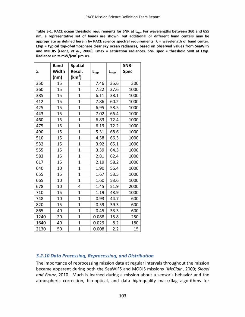
PACE Mission Science Definition Team Report
Table 3-1. PACE ocean threshold requirements for SNR at Ltyp. For wavelengths between 360 and 655 nm, a representative set of bands are shown, but additional or different band centers may be appropriate as defined herein by PACE science spectral requirements. λ = wavelength of band center. Ltyp = typical top-of-atmosphere clear sky ocean radiances, based on observed values from SeaWiFS and MODIS [Franz, et al., 2006]. Lmax = saturation radiances. SNR spec = threshold SNR at Ltyp. Radiance units mW/(cm2 µm sr).
λ
Band Width (nm)
Spatial Resol. (km2)
Ltyp
Lmax
SNR- Spec
350 15 1 7.46 35.6 300 360 15 1 7.22 37.6 1000 385 15 1 6.11 38.1 1000 412 15 1 7.86 60.2 1000 425 15 1 6.95 58.5 1000 443 15 1 7.02 66.4 1000 460 15 1 6.83 72.4 1000 475 15 1 6.19 72.2 1000 490 15 1 5.31 68.6 1000 510 15 1 4.58 66.3 1000 532 15 1 3.92 65.1 1000 555 15 1 3.39 64.3 1000 583 15 1 2.81 62.4 1000 617 15 1 2.19 58.2 1000 640 10 1 1.90 56.4 1000 655 15 1 1.67 53.5 1000 665 10 1 1.60 53.6 1000 678 10 4 1.45 51.9 2000 710 15 1 1.19 48.9 1000 748 10 1 0.93 44.7 600 820 15 1 0.59 39.3 600 865 40 1 0.45 33.3 600 1240 20 1 0.088 15.8 250 1640 40 1 0.029 8.2 180 2130 50 1 0.008 2.2 15
3.2.10 Data Processing, Reprocessing, and Distribution The importance of reprocessing mission data at regular intervals throughout the mission became apparent during both the SeaWiFS and MODIS missions [McClain, 2009; Siegel and Franz, 2010]. Much is learned during a mission about a sensor’s behavior and the atmospheric correction, bio-optical, and data high-quality mask/flag algorithms for
103
PACE Mission Science Definition Team Report
converting Lw into ocean color products. Data reprocessing is needed to adjust for the following changes: (1) calibration coefficients due to sensor degradation, (2) in-water and atmospheric correction algorithms resulting from validation results, and (3) availability of new algorithms for improved data products. In addition, it takes many match-ups before a vicarious calibration can achieve the desired accuracy and stability for the sensor’s gain factor. Therefore, data processing and product generation cannot be expected to produce high-quality products at the beginning of a mission. For all these reasons, data product quality will improve as more is learned about a sensor’s behavior and as a result of reprocessing. For example, the initial processing of SeaWiFS imagery yielded negative values for water-leaving radiance for continental shelf waters in the band centered at 412 nm and depressed values at 443 nm. This difficult problem was not fully resolved until the data were reprocessed many times [e.g., Patt et al., 2003; McClain, 2009]. In 2009, the reprocessing of the MODIS-Aqua dataset corrected another, much more subtle drift in the 412 nm water-leaving radiance band, which had resulted in an apparent dramatic increase in CDOM concentration in the open ocean [Maritorena et al., 2010].
Reprocessing of ocean color datasets is also critical for developing decadal-scale records across multiple missions. Antoine et al. [2005] developed a decadal-scale ocean color data record by linking the CZCS data record to the SeaWiFS era. Key to their approach was the reprocessing of both datasets using similar algorithms and sources. The resulting decadal ocean color time series shows many interesting climate patterns supporting their approach [Martinez et al., 2009]. Thus, it is likely that the best approach to creating multi-decadal ocean color data products is the simultaneous reprocessing of multiple ocean color missions with similar algorithms and the same vicarious calibration sources, if possible [Siegel and Franz, 2010]. Based on experience with heritage data sets, it is strongly recommended that the PACE mission be designed and resources (people, equipment, funding, etc.) be dedicated to a capacity for full data reprocessing at a minimum frequency of 1–2 times annually. Furthermore, it is strongly recommended that the PACE mission establish a dedicated and consistent team for data processing, reprocessing, and distribution, as was employed during the SeaWiFS mission. It should also be noted that additional reprocessing capabilities are needed in support of calibration and algorithm investigations and testing (see section 4.6).
The PACE ocean instrument has the potential to create a data set with unprecedented spectral resolution, spectral coverage, and spatial resolution and coverage. To create these observations, there are many potential tradeoffs that must be considered regarding desired spatial/spectral resolutions and required signal levels. This suggests that the user, in theory, could have much greater control over the data products produced and, in particular, the aggregation of spectral bands and spatial observations. This means that the PACE data processing system will benefit from being as flexible as possible to enable more user control than for past NASA ocean mission data sets. Providing both traditional data products/formats (cf., nRw, Chl and IOPs in a traditional Level 2 [L2] and L3 formats) and an ability for users to create their own products for
104
PACE Mission Science Definition Team Report
their particular applications from the suite of full spectral and spatial Level 1B (L1B) observations should be viewed as an objective for PACE. The former data system may be thought of as a next-generation version of SeaDAS. In this way, we envision the scientific and application communities getting the most value from the investment that is PACE.
Measurements made by the PACE ocean radiometer will, as discussed throughout this document, have broad and interdisciplinary value for science and applications. The impact of the mission will be greatest if data latency is minimized. For many applications, a data latency of 3 hours supports near-real-time analyses, and experience with MODIS ocean color data has demonstrated that this latency period is achievable. Rapid access to PACE data is important for field studies supporting the mission and investigating transient events, such as the development of harmful algal blooms. Near-real-time data access is also valuable for fisheries applications and emergency response (e.g., oil spill monitoring). In addition, experience with MODIS-TERRA and MODIS-AQUA has shown that direct broadcast of ocean color data further improves the impact of an ocean color mission. Direct broadcast provides minimal latency, enhances access to data globally, fosters international scientific collaborations, helps the U.S. to support international agreements, and improves sensor calibration and validation efforts. Furthermore, investigators receiving direct broadcast data experience hands-on training in data processing, thereby developing a deeper understanding of remote sensing physics and fostering education of the next generation of algorithm developers. Data latency recommendations for PACE are thus:
• Latency Threshold Requirement: 3-hour data latency (95% confidence) for the distribution of preliminary L1B data, 3-hour latency for Level 2 products, and direct broadcast of a subset of aggregate spectral bands.
• Latency Goal: 0.5-hour latency for radiances and level 2 products (including masks and flags) and direct broadcast of PACE data at full spectral resolution (5 nm).
Threshold Requirement: Capacity for full reprocessing of PACE data at a minimum frequency of 1–2 times annually. An ability for users to create their own products for their particular applications from the suite of full spectral and spatial Level 1B data; i.e., mission support for a software package (the analog, or the basis, would be SeaDAS for SeaWiFS, MODIS and other). Three-hour data latency for L1B data and Level 2 products. Direct broadcast of aggregate bands.
Goal: 0.5-hour latency for radiances and level 2 products (including masks and flags) and direct broadcast of PACE data at full spectral resolution (5 nm).
105
PACE Mission Science Definition Team Report
3.2.11 Summary of PACE Ocean Science Measurement Requirements In this section of the SDT report, we have defined specific threshold ocean science requirements for the PACE ocean radiometer and have identified additional capabilities (goals) that could extend the scientific contributions of the mission. The threshold requirements derive directly from the science objectives and approaches detailed in section 3.2, and reflect the mission’s primary focus on achieving global ocean climate-quality data for extending the heritage ocean color record and addressing outstanding science issues inaccessible to the restricted capabilities of these earlier sensors. Throughout this section, we have identified specific approaches for meeting the measurement requirements based on experience with heritage sensors, but have also noted that alternative approaches should be considered if their effectiveness is clearly demonstrated. To aid NASA in its evaluation of PACE, we provide below in Table 3-2 a summary of the threshold ocean requirements deemed essential to achieve PACE minimum science objectives. Note that these threshold requirements are not ranked, as they must all be met by the selected PACE instrument. In addition, we also provide a Science Traceability Matrix (STM) in Table 3-1 for the threshold PACE ocean science mission. Finally, we provide a summary list of additional PACE goals in section 3.2.12. We emphasize that achieving any of these goals should not be viewed as exchangeable with the essential threshold requirements in Table 3-2, or be considered if they compromise any of the essential threshold requirements for the mission.
106
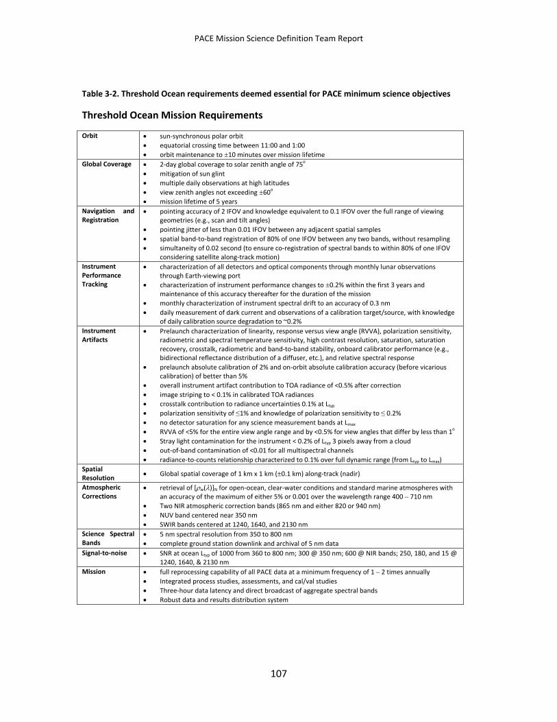
PACE Mission Science Definition Team Report
Table 3-2. Threshold Ocean requirements deemed essential for PACE minimum science objectives
Threshold Ocean Mission Requirements
Orbit • sun-synchronous polar orbit • equatorial crossing time between 11:00 and 1:00 • orbit maintenance to ±10 minutes over mission lifetime
Global Coverage • 2-day global coverage to solar zenith angle of 75o • mitigation of sun glint • multiple daily observations at high latitudes • view zenith angles not exceeding ±60o • mission lifetime of 5 years
Navigation and Registration
• pointing accuracy of 2 IFOV and knowledge equivalent to 0.1 IFOV over the full range of viewing geometries (e.g., scan and tilt angles)
• pointing jitter of less than 0.01 IFOV between any adjacent spatial samples • spatial band-to-band registration of 80% of one IFOV between any two bands, without resampling • simultaneity of 0.02 second (to ensure co-registration of spectral bands to within 80% of one IFOV
considering satellite along-track motion) Instrument Performance Tracking
• characterization of all detectors and optical components through monthly lunar observations through Earth-viewing port
• characterization of instrument performance changes to ±0.2% within the first 3 years and maintenance of this accuracy thereafter for the duration of the mission
• monthly characterization of instrument spectral drift to an accuracy of 0.3 nm • daily measurement of dark current and observations of a calibration target/source, with knowledge
of daily calibration source degradation to ~0.2% Instrument Artifacts
• Prelaunch characterization of linearity, response versus view angle (RVVA), polarization sensitivity, radiometric and spectral temperature sensitivity, high contrast resolution, saturation, saturation recovery, crosstalk, radiometric and band-to-band stability, onboard calibrator performance (e.g., bidirectional reflectance distribution of a diffuser, etc.), and relative spectral response
• prelaunch absolute calibration of 2% and on-orbit absolute calibration accuracy (before vicarious calibration) of better than 5%
• overall instrument artifact contribution to TOA radiance of <0.5% after correction • image striping to < 0.1% in calibrated TOA radiances • crosstalk contribution to radiance uncertainties 0.1% at Ltyp • polarization sensitivity of ≤1% and knowledge of polarization sensitivity to ≤ 0.2% • no detector saturation for any science measurement bands at Lmax • RVVA of <5% for the entire view angle range and by <0.5% for view angles that differ by less than 1o • Stray light contamination for the instrument < 0.2% of Ltyp 3 pixels away from a cloud • out-of-band contamination of <0.01 for all multispectral channels • radiance-to-counts relationship characterized to 0.1% over full dynamic range (from Ltyp to Lmax)
Spatial Resolution • Global spatial coverage of 1 km x 1 km (±0.1 km) along-track (nadir)
Atmospheric Corrections
• retrieval of [ρw(λ)]N for open-ocean, clear-water conditions and standard marine atmospheres with an accuracy of the maximum of either 5% or 0.001 over the wavelength range 400 – 710 nm
• Two NIR atmospheric correction bands (865 nm and either 820 or 940 nm) • NUV band centered near 350 nm • SWIR bands centered at 1240, 1640, and 2130 nm
Science Spectral Bands
• 5 nm spectral resolution from 350 to 800 nm • complete ground station downlink and archival of 5 nm data
Signal-to-noise • SNR at ocean Ltyp of 1000 from 360 to 800 nm; 300 @ 350 nm; 600 @ NIR bands; 250, 180, and 15 @ 1240, 1640, & 2130 nm
Mission • full reprocessing capability of all PACE data at a minimum frequency of 1 – 2 times annually • Integrated process studies, assessments, and cal/val studies • Three-hour data latency and direct broadcast of aggregate spectral bands • Robust data and results distribution system
107
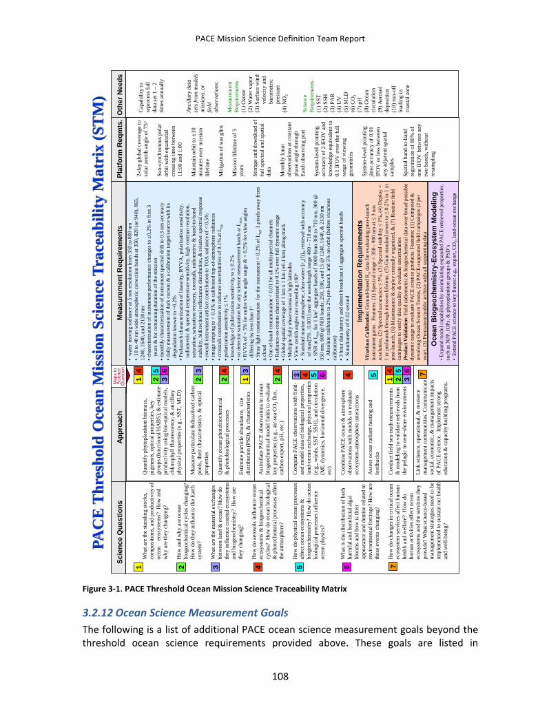
PACE Mission Science Definition Team Report
Figure 3-1. PACE Threshold Ocean Mission Science Traceability Matrix
3.2.12 Ocean Science Measurement Goals The following is a list of additional PACE ocean science measurement goals beyond the threshold ocean science requirements provided above. These goals are listed in
PAC
E T
hres
hold
Oce
an M
issi
on S
cien
ce T
race
abili
ty M
atri
x (S
TM
)
Impl
emen
tatio
n R
equi
rem
ents
Vica
riou
s Cal
ibra
tion:
Gro
und-
base
d R
rsda
ta fo
r eva
luat
ing
post
-laun
ch
inst
rum
ent g
ains
. Fe
atur
es: (
1) S
pect
ral r
ange
= 3
50 -
900
nm a
t ≤ 3
nm
re
solu
tion,
(2) S
pect
ral a
ccur
acie
s ≤ 5
%, (
3) S
pect
ral s
tabi
lity
≤ 1%
, (4)
Dep
loy
= 1
yrpr
elau
nch
thro
ugh
mis
sion
life
time,
(5) G
ain
stan
dard
erro
rs to
≤ 0
.2%
in 1
yr
post
-laun
ch, (
6) M
aint
enan
ce &
dep
loy
cent
rally
org
aniz
ed, &
(7) R
outin
e fie
ld
cam
paig
ns to
ver
ify d
ata
qual
ity &
eva
luat
e un
certa
intie
sPr
oduc
t Val
idat
ion:
Fie
ld ra
diom
etric
& b
ioge
oche
mic
al d
ata
over
bro
ad p
ossi
ble
dyna
mic
rang
e to
eva
luat
e PA
CE
scie
nce
prod
ucts
. Fea
ture
s: (1
) Com
pete
d &
re
volv
ing
Oce
an S
cien
ce T
eam
s, (2
) PA
CE-
supp
orte
d fie
ld c
ampa
igns
(2 p
er
year
), (3
) Per
man
ent/p
ublic
arch
ive
with
all
supp
ortin
g da
ta
Oce
an B
ioge
oche
mis
try-
Ecos
yste
m M
odel
ing
•Exp
and
mod
el c
apab
ilitie
s by
assi
mila
ting
expa
nded
PA
CE
retri
eved
pro
perti
es,
such
as N
PP, I
OPs
, & p
hyto
plan
kton
gro
ups &
PSD
’s•
Exte
nd P
AC
E sc
ienc
e to
key
flux
es: e
.g.,
expo
rt, C
O2,
land
-oce
an e
xcha
nge
1 2 3 4 5 6
Wha
t are
the
stan
ding
stoc
ks,
com
posi
tions
, and
pro
duct
ivity
of
ocea
n
ecos
yste
ms?
How
and
w
hy a
re th
ey c
hang
ing?
How
and
why
are
oce
an
biog
eoch
emic
al c
ycle
s ch
angi
ng?
How
do
they
influ
ence
the
Earth
sy
stem
?
Wha
t are
the
mat
eria
l exc
hang
es
betw
een
land
& o
cean
? H
ow d
o th
ey in
fluen
ce c
oast
al e
cosy
stem
s an
d bi
ogeo
chem
istry
? H
ow a
re
they
cha
ngin
g?
How
do
aero
sols
influ
ence
oce
an
ecos
yste
ms
& b
ioge
oche
mic
al
cycl
es?
How
do
ocea
n bi
olog
ical
&
pho
toch
emic
al p
roce
sses
aff
ect
the
atm
osph
ere?
How
do
phys
ical
oce
an p
roce
sses
af
fect
oce
an ec
osys
tem
s &
bi
ogeo
chem
istry
? H
ow d
o oc
ean
biol
ogic
al p
roce
sses
influ
ence
oc
ean
phys
ics?
Wha
t is t
he d
istri
butio
n of
bot
h ha
rmfu
l and
ben
efic
ial a
lgal
bl
oom
s an
d ho
w is
thei
r ap
pear
ance
and
dem
ise
rela
ted
to
envi
ronm
enta
l for
cing
s? H
ow a
re
thes
e ev
ents
cha
ngin
g?
How
do
chan
ges i
n cr
itica
l oce
an
ecos
yste
m s
ervi
ces a
ffec
t hum
an
heal
th a
nd w
elfa
re?
How
do
hum
an a
ctiv
ities
aff
ect o
cean
ec
osys
tem
s an
d th
e se
rvic
es th
ey
prov
ide?
Wha
t sci
ence
-bas
ed
man
agem
ent s
trate
gies
nee
d to
be
impl
emen
ted
to su
stai
n ou
r hea
lth
and
wel
l-bei
ng?
7
Qua
ntify
phy
topl
ankt
on b
iom
ass,
pigm
ents
, opt
ical
pro
perti
es, k
ey
grou
ps (f
unct
iona
l/HA
BS)
, & e
stim
ate
prod
uctiv
ity u
sing
bio
-opt
ical
mod
els,
chlo
roph
yll f
luor
esce
nce,
& a
ncill
ary
phys
ical
pro
perti
es (e
.g.,
SST,
MLD
)
Mea
sure
par
ticul
ate &
diss
olve
d ca
rbon
po
ols,
thei
r cha
ract
eris
tics
& o
ptic
al
prop
ertie
s
Qua
ntify
oce
an p
hoto
bioc
hem
ical
&
pho
tobi
olog
ical
pro
cess
es
Estim
ate
parti
cle
abun
danc
e, s
ize
dist
ribut
ion
(PSD
), &
cha
ract
eris
tics
Ass
imila
te P
AC
E ob
serv
atio
ns in
oce
an
biog
eoch
emic
al m
odel
fiel
ds to
eva
luat
e ke
y pr
oper
ties (
e.g.
, air-
sea
CO
2flu
x,
carb
on ex
port,
pH
, etc
.)
Com
pare
PA
CE
obse
rvat
ions
with
fiel
d-an
d m
odel
dat
a of
bio
logi
cal p
rope
rties
, la
nd-o
cean
exch
ange
, phy
sica
l pro
perti
es
(e.g
., w
inds
, SST
, SSH
), an
d ci
rcul
atio
n (M
L dy
nam
ics,
horiz
onta
l div
erge
nce,
et
c)
Com
bine
PA
CE
ocea
n &
atm
osph
ere
obse
rvat
ions
with
mod
els t
o ev
alua
te
ecos
yste
m-a
tmos
pher
e in
tera
ctio
ns
Ass
ess
ocea
n ra
dian
t hea
ting
and
feed
back
s
Con
duct
fiel
d se
a-tru
th m
easu
rem
ents
&
mod
elin
g to
val
idat
e re
triev
als f
rom
th
e pe
lagi
c to
nea
r-sho
re e
nviro
nmen
ts
Link
scie
nce,
ope
ratio
nal,
& re
sour
ce
man
agem
ent c
omm
uniti
es. C
omm
unic
ate
soci
al, e
cono
mic
, & m
anag
emen
t im
pact
s of
PA
CE
scie
nce.
Im
plem
ent s
trong
ed
ucat
ion
& c
apac
ity b
uild
ing
prog
ram
s.
1 2 2 22
3 33 44 4 4 5553
46
1 2 3
4 5 66 7
1
2-da
y gl
obal
cov
erag
e to
so
lar z
enith
ang
le o
f 75o
Sun-
sync
hron
ous p
olar
or
bit w
ith e
quat
oria
l cr
ossi
ng ti
me
betw
een
11:0
0 an
d 1:
00
Mai
ntai
n or
bit t
o ±1
0 m
inut
es o
ver m
issi
on
lifet
ime
Miti
gatio
n of
sun
glin
t
Mis
sion
life
time
of 5
ye
ars
Stor
age
and
dow
nloa
d of
fu
ll sp
ectra
l and
spat
ial
data
Mon
thly
luna
r ob
serv
atio
ns a
t con
stan
t ph
ase
angl
e th
roug
h Ea
rth o
bser
ving
por
t
Syst
em-le
vel p
oint
ing
accu
racy
of 2
IFO
V a
nd
know
ledg
e eq
uiva
lent
to
0.1
IFO
V o
ver t
he fu
ll ra
nge
of v
iew
ing
geom
etrie
s
Syst
em-le
vel p
oint
ing
jitte
r acc
urac
y of
0.0
1 IF
OV
or l
ess b
etw
een
any
adja
cent
spat
ial
sam
ples
Spat
ial b
and-
to-b
and
regi
stra
tion
of 8
0% o
f on
e IF
OV
bet
wee
n an
y tw
o ba
nds,
with
out
resa
mpl
ing
Cap
abili
ty to
re
proc
ess f
ull
data
set 1
–2
times
ann
ually
Anci
llary
dat
a se
ts fr
om m
odel
s m
issi
ons,
or
field
ob
serv
atio
ns:
Mea
sure
men
tR
equi
rem
ents
(1) O
zone
(2) W
ater
vap
or(3
) Sur
face
win
dve
loci
ty a
ndba
rom
etric
pres
sure
(4) N
O2
Scie
nce
Req
uire
men
ts(1
) SST
(2) S
SH(3
) PA
R(4
) UV
(5) M
LD(6
) CO
2(7
) pH
(8) O
cean
ci
rcul
atio
n(9
) Aer
osol
de
posi
tion
(10)
run-
off
load
ing
in
coas
tal z
one
•w
ater
leav
ing
radi
ance
at 5
nm
reso
lutio
n fro
m35
0to
800
nm
•10
to 4
0 nm
wid
e at
mos
pher
ic co
rrec
tion
band
s at 3
50, 8
20 (o
r 940
), 86
5,
1240
, 164
0, an
d 21
30 n
m•c
hara
cter
izat
ion
of in
stru
men
t per
form
ance
cha
nges
to ±
0.2%
in fi
rst 3
year
s & fo
r rem
aini
ng d
urat
ion
of th
e m
issi
on•m
onth
ly c
hara
cter
izat
ion
of in
stru
men
t spe
ctra
l drif
t to
0.3
nm a
ccur
acy
•dai
ly m
easu
rem
ent o
f dar
k cu
rren
t & a
cal
ibra
tion
targ
et/s
ourc
e with
its
degr
adat
ion
know
n to
~0.
2%•P
rela
unch
char
acte
rizat
ion
of li
near
ity, R
VV
A, p
olar
izat
ion
sens
itivi
ty,
radi
omet
ric &
spec
tral t
empe
ratu
re se
nsiti
vity
, hig
h co
ntra
st re
solu
tion,
satu
ratio
n, sa
tura
tion
reco
very
, cro
ssta
lk, r
adio
met
ric &
ban
d-to
-ban
dst
abili
ty, b
idire
ctio
nal r
efle
ctan
ce d
istri
butio
n, &
rela
tive
spec
tral r
espo
nse
•ove
rall
inst
rum
ent a
rtifa
ct c
ontri
butio
n to
TO
A ra
dian
ce o
f < 0
.5%
•im
age
strip
ing
to <
0.1
% in
cal
ibra
ted
top-
of-a
tmos
pher
e ra
dian
ces
•cro
ssta
lk c
ontri
butio
n to
radi
ance
unc
erta
intie
s of 0
.1%
at L
typ
•pol
ariz
atio
n se
nsiti
vity
≤ 1
%•k
now
ledg
e of
pol
ariz
atio
n se
nsiti
vity
to ≤
0.2
%•n
o de
tect
or sa
tura
tion
for a
ny sc
ienc
e m
easu
rem
ent b
ands
at L
max
•RV
VA
of <
5%
for e
ntire
vie
w a
ngle
rang
e &
< 0
.5%
for v
iew
ang
les
diffe
ring
by le
ss th
an 1
o
•Stra
y lig
ht c
onta
min
atio
n fo
r the
inst
rum
ent <
0.2
% o
f Lty
p3
pixe
ls aw
ay fr
om
a cl
oud
•Out
-of-b
and
cont
amin
atio
n <
0.01
for a
ll m
ultis
pect
ral c
hann
els
•Rad
ianc
e-to
-cou
nts c
hara
cter
ized
to 0
.1%
ove
r ful
l dyn
amic
rang
e •G
loba
l spa
tial c
over
age
of 1
km
x 1
km
(±0.
1 km
) alo
ng-tr
ack
•Mul
tiple
dai
ly o
bser
vatio
ns at
hig
h la
titud
es•V
iew
zen
ith an
gles
not
exc
eedi
ng ±
60o
•St
anda
rd m
arin
e at
mos
pher
e, cl
ear-w
ater
[rw(
l)]N
retri
eval
with
acc
urac
yof
max
[5%
, 0.
001]
ove
r the
wav
elen
gth
rang
e 40
0 –
710
nm•
SNR
at L
typ
for 1
km
2ag
greg
ate
band
s of 1
000
from
360
to 7
10 n
m; 3
00 @
35
0 nm
; 600
@ N
IR b
ands
; 250
, 180
, and
15
@ 1
240,
164
0, &
213
0 nm
•A
bsol
ute
calib
ratio
n to
2%
pre
-laun
ch a
nd 5
% o
n-or
bit (
befo
re v
icar
ious
ca
libra
tion)
•3 h
our d
ata
late
ncy
and
dire
ct b
road
cast
of a
ggre
gate
spec
tral b
ands
•Si
mul
tane
ity o
f 0.0
2 se
cond
Map
s to
Sci
ence
Que
stio
nSc
ienc
e Q
uest
ions
A
ppro
ach
M
easu
rem
ent R
equi
rem
ents
Pl
atfo
rm R
eqm
ts.
Oth
er N
eeds
108
PACE Mission Science Definition Team Report
alphabetical order according to topic (italics) and thus are not listed according to priority. These goals do not represent a 'trade space' with threshold requirements, but are beneficial to the mission if achieved in addition to the minimum mission requirements described above in Table 3-2.
• Accuracy: Retrieval of normalized [ρw(λ)]N for open-ocean, clear-water conditions and standard marine atmospheres with an accuracy of the maximum of either 10% or 0.002 over the wavelength range of 350 – 395 nm
• Aerosol heights: Identified approach or measurement capacity for evaluating/measuring aerosol vertical distributions and type for improved atmospheric corrections
• Atmospheric correction: SWIR atmospheric correction band at 2130 nm with a SNR of 100
• Coverage: 1-day global coverage
• Coverage: Coverage to a solar zenith angle >75o
• Crossing time: Noon equatorial crossing time (±10 min)
• Data Latency: 0.5 hour data latency and direct broadcast of 5 nm resolution data
• Instrument artifact: Overall instrument artifact contribution to top of the atmosphere (TOA) radiance retrievals of <0.2%
• Navigation and Registration: pointing knowledge of 0.05 Instantaneous Field of View (IFOV); band-to-band registration of 90% of one IFOV; simultaneity of 0.01 second
• Nitrogen dioxide: Identified approach for characterizing NO2 and ozone concentrations at sufficient accuracy for improving atmospheric corrections
• Mission lifetime: 10 years
• Performance changes: Characterization of instrument performance changes to ±0.1% within 3 years and maintenance of this accuracy thereafter
• Saturation: No detector saturation for any science measurement bands up to 1.2 × Lmax
• Signal-to-noise: SNR for bio-optical science bands and/or atmospheric correction bands greater than those shown in Table 3-1 and Appendix A
• Spatial resolution: Spatial resolution of 1 km2 (±10%) at all angles across track
109
PACE Mission Science Definition Team Report
• Spatial resolution: Along-track spatial resolution of 250 m x 250 m to <1 km2 for inland, estuarine, coastal, and shelf area retrievals for all bands or a subset of bands
• Spectral coverage: 5 nm spectral coverage from 800 to 900 nm
• Spectral sub-sampling: Spectral sub-sampling at ~1-2 nm resolution from 655 to 710 nm for refined characterization of the chlorophyll fluorescence spectrum
3.2.13 Atmospheric Correction Topics Relevant to PACE Ocean Retrievals One of the unique aspects of the PACE mission is its cross-disciplinary philosophy. With respect to ocean and aerosol communities, the interdisciplinary nature of the mission reflects both joint science questions (e.g., iron fertilization through dust deposition) and interdependencies in property retrievals. Regarding the latter issue, key questions include (1) how much aerosol-type information is needed to significantly improve atmospheric corrections for ocean parameter retrievals, and (2) where and when are these advanced aerosol characterizations most critical. The atmospheric correction is essential for deriving accurate water-leaving radiances [IOCCG, 2010], and has been traditionally performed by constraining AOD and aerosol type using a pair of NIR wavelengths (although SWIR bands may be employed for turbid water conditions) (see section 3.2.7). At these wavelengths, the ocean surface tends to be dark. Atmospheric AOD and absorbing AOD (AAOD) properties derived at these wavelengths are then extrapolated to the blue (and for PACE, also the near-UV) wavelengths that are used to derive ocean ecosystem and biogeochemical properties [Gordon and Wang, 1994; Wang, 2007]. Importantly, errors in the atmospheric correction generally increase from longer to shorter wavelengths, due to the optical properties of both aerosols and atmospheric gases [IOCCG, 2010].
Figure 3-2 provides an initial illustration of the ocean color–aerosol challenge. In this figure, spectral influences of chlorophyll-a, CDOM, and aerosols are presented over the 350–900 nm spectral range, where TOA radiances are calculated from an application of Knut Stamnes’ coupled atmosphere-ocean computer code [Jin and Stamnes, 1994]. TOA radiances for pure water conditions (including atmospheric gases, but without aerosols, CDOM, or chlorophyll-a) are subtracted for each case presented, followed by normalization to produce reflectances [i.e. ρ = π L / E(solar)]. The left panel in Figure 3-2 shows spectral changes associated with chlorophyll concentrations ranging from 0.5 to 1.0 mg m-3, and indicates that ρ values on the order of 0.001 need to be determined from the observed radiances in order to resolve the different chlorophyll-a amounts. This value is consistent with the 0.001 accuracy specification discussed by Gordon and Wang [1994]. The middle panel of Figure 3-2 shows that CDOM primarily influences the NUV and shortest visible wavelengths. The right panel shows (for the pure water case only) results for a purely scattering aerosol and an absorbing aerosol, with the former aerosol type increasing TOA radiances more than the latter (as expected). This
110
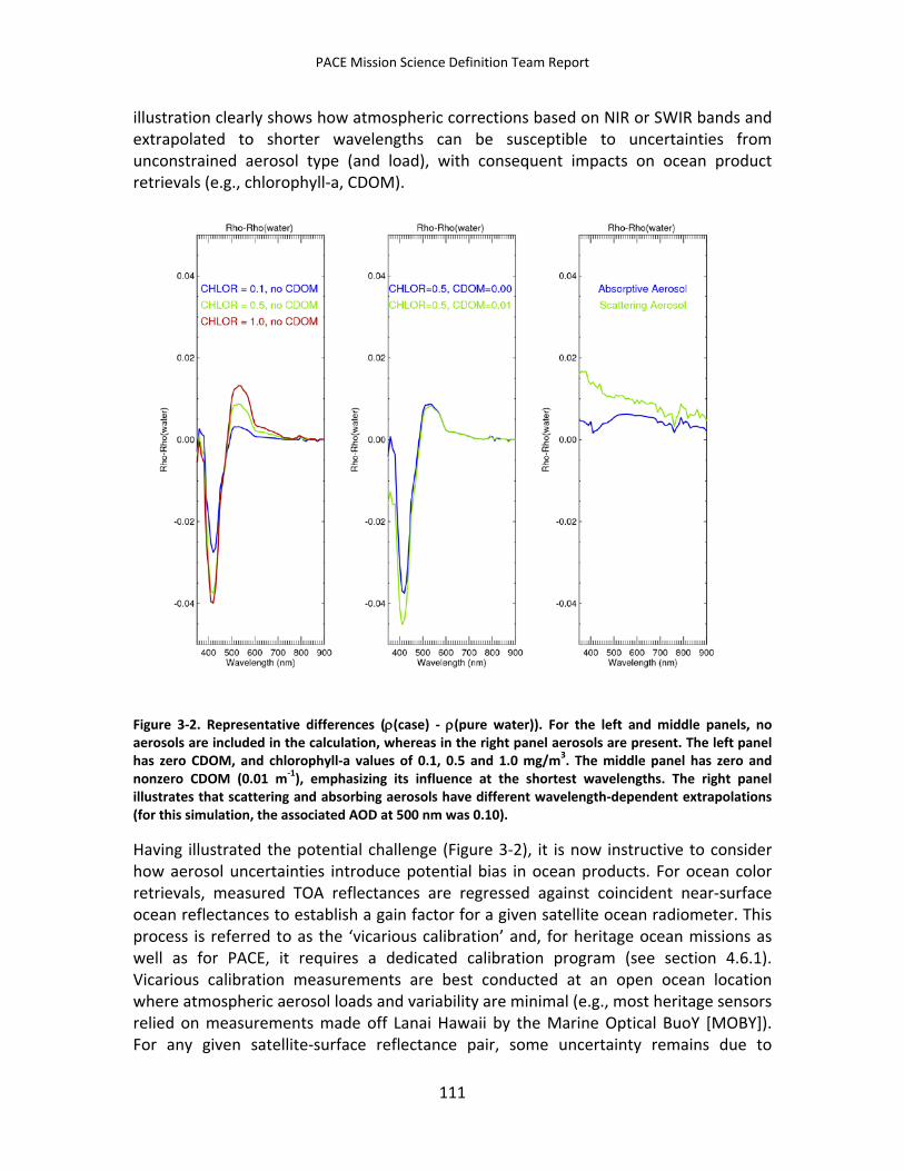
PACE Mission Science Definition Team Report
illustration clearly shows how atmospheric corrections based on NIR or SWIR bands and extrapolated to shorter wavelengths can be susceptible to uncertainties from unconstrained aerosol type (and load), with consequent impacts on ocean product retrievals (e.g., chlorophyll-a, CDOM).
Figure 3-2. Representative differences (ρ(case) - ρ(pure water)). For the left and middle panels, no aerosols are included in the calculation, whereas in the right panel aerosols are present. The left panel has zero CDOM, and chlorophyll-a values of 0.1, 0.5 and 1.0 mg/m3. The middle panel has zero and nonzero CDOM (0.01 m-1), emphasizing its influence at the shortest wavelengths. The right panel illustrates that scattering and absorbing aerosols have different wavelength-dependent extrapolations (for this simulation, the associated AOD at 500 nm was 0.10).
Having illustrated the potential challenge (Figure 3-2), it is now instructive to consider how aerosol uncertainties introduce potential bias in ocean products. For ocean color retrievals, measured TOA reflectances are regressed against coincident near-surface ocean reflectances to establish a gain factor for a given satellite ocean radiometer. This process is referred to as the ‘vicarious calibration’ and, for heritage ocean missions as well as for PACE, it requires a dedicated calibration program (see section 4.6.1). Vicarious calibration measurements are best conducted at an open ocean location where atmospheric aerosol loads and variability are minimal (e.g., most heritage sensors relied on measurements made off Lanai Hawaii by the Marine Optical BuoY [MOBY]). For any given satellite-surface reflectance pair, some uncertainty remains due to
111
PACE Mission Science Definition Team Report
unconstrained aerosol impacts. However, this uncertainty is minimized by collecting many paired observations over all seasons, such that the time series of observations converges on a single gain factor. For the SeaWiFS mission, this convergence required more than two years. Once a reliable gain factor is established (for PACE the goal is to achieve this gain within the first year of operations), it is used to scale TOA reflectances measured elsewhere. This vicarious calibration procedure is not impacted by global variability in atmospheric aerosols, although some error can still exist if an aerosol bias persists in all the field-satellite data pairs. Historically, atmospheric measurements have not accompanied the ocean vicarious calibration measurements. For PACE, including these additional observations (e.g., sun-photometer measurements) is advised.
Once a sensor gain factor is determined, the resultant calibrated global data set of TOA reflectances must then be corrected for local atmospheric conditions to retrieve water-leaving radiances, and it is in this procedure (currently based on the NIR and SWIR approach described above) that errors can arise from uncertainties in aerosol characteristics. In addition to the magnitude of the AOD itself, spectral AOD and AAOD ‘slopes’ of different aerosol types need to be taken into account for maximum aerosol correction accuracy [Ahmad et al., 2010]. Key aerosol types that dominate at different locations and in different seasons over the ocean include Saharan dust, Gobi dust, different types of organic ("brown") carbon (e.g., most wildfire smoke and urban pollution particles), black carbon (e.g. from diesel and some fire combustion products), sea salt, and sulfate particles.
The shortest measurement band in heritage ocean color missions (e.g., SeaWiFS, MODIS and MERIS) has been near 410 nm. As noted above, uncertainties in atmospheric corrections increase with decreasing wavelength, and at 410 nm, errors due to uncertainties in aerosol amount, type, and vertical distribution can be significant. For PACE, ocean retrievals will be extended into the NUV down to 350 nm. This extension may necessitate a re-evaluation of the atmospheric correction approach due to difference in atmospheric optical properties between the UV and visible wavelengths (specifically, increased contribution from absorbing aerosols, as well as impacts of scattering aerosols). An evaluation is also needed of uncertainties associated with atmospheric pressure effects on the gas-scattering contribution to the TOA signal. Retrieval of ocean CDOM may be a particularly challenging issue for some regions and times. Specifically, the spectral shape of absorption by some aerosol types is similar to that of oceanic CDOM, both of which are most strongly absorbing in the UV. Inaccurate separation of these different components can result in significant biases in CDOM retrievals (particularly, for example, in coastal regions with high CDOM and low suspended sediment concentration), although the extent of this issue has not yet been quantified.
The global average AOD is ~0.14 at mid-visible wavelengths, with a tendency to increase with decreasing wavelength. Near many coastal areas and under spatially extensive aerosol plumes, mid-visible AODs can reach 0.4 or greater. In some cases, these large plumes can be carried far downwind from their sources to overlie significant ocean
112
PACE Mission Science Definition Team Report
areas. The standard practice in ocean color data processing is to flag pixels with AODs > 0.3, but this flagging process can sometimes underestimate aerosol loads, resulting in assumed valid pixels with water-leaving radiance retrievals that have large errors. Thus, one fundamental, quantitative question regarding atmospheric corrections is: How well can we recognize and flag cases where good atmospheric corrections cannot be made? In addition, some important science questions (e.g., dust deposition impacts on plankton) would benefit from ocean retrievals under higher aerosol loads, so actually achieving a valid atmospheric correction under these conditions (rather than just flagging the data) should be a pursuit during the PACE mission. Example regions where aerosol contributions to TOA reflectances can be significant include the north Atlantic downwind of the Sahara (as far west as the Caribbean) during boreal spring and summer; the Equatorial and South Atlantic during the burning seasons in sub-Saharan, central, and southern Africa; the western Pacific during the spring dust season, winter pollution season, and during biomass burning episodes; and the Bay of Bengal during winter and pre-monsoon.
Another fundamental, quantitative question is how good an atmospheric correction is good enough, when significant aerosols are present? The answer to this question likely varies with the parameter being retrieved. Nevertheless, several points must be addressed to obtain a meaningful answer:
a) What are the value ranges for the key PACE ocean parameters and with what sensitivity must they be measured? While the key ocean parameters have been discussed extensively in this document and their baseline and threshold ranges are given in Appendix A, the required sensitivities for their retrievals are not yet quantitatively defined.
b) What channels will be used to retrieve each ocean color parameter and, given the sensitivities mentioned in (a), with what sensitivity do the ocean surface spectral radiances need to be retrieved? The channels for each parameter are described in sections 2.2.2 and 3.2.8, but required ocean surface spectral radiance sensitivities are not yet quantitatively defined.
c) Appropriate radiative transfer tools are available, as well as state-of-the-art aerosol and ocean surface optical models [e.g., Ahmad et al., 2010; Chowdhary et al., 2012; Wang, 2007; Jin and Stamnes, 1994]. Based upon ocean surface spectral radiance sensitivity requirements from (b), these tools can be used to simulate TOA radiances under different assumed aerosol and surface conditions, establishing the aerosol type constraints needed to provide atmospheric corrections to the required degree of accuracy to obtain the ocean color parameters.
The forward calculations described in (a) and (b) above can help establish measurement requirements for atmospheric correction by assessing sensitivity, but a complete analysis also requires assessing uncertainties associated with assumptions regarding
113
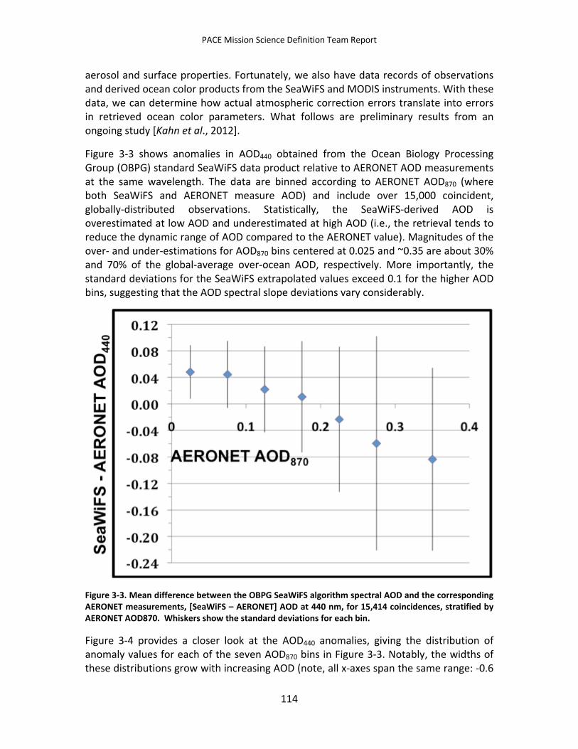
PACE Mission Science Definition Team Report
aerosol and surface properties. Fortunately, we also have data records of observations and derived ocean color products from the SeaWiFS and MODIS instruments. With these data, we can determine how actual atmospheric correction errors translate into errors in retrieved ocean color parameters. What follows are preliminary results from an ongoing study [Kahn et al., 2012].
Figure 3-3 shows anomalies in AOD440 obtained from the Ocean Biology Processing Group (OBPG) standard SeaWiFS data product relative to AERONET AOD measurements at the same wavelength. The data are binned according to AERONET AOD870 (where both SeaWiFS and AERONET measure AOD) and include over 15,000 coincident, globally-distributed observations. Statistically, the SeaWiFS-derived AOD is overestimated at low AOD and underestimated at high AOD (i.e., the retrieval tends to reduce the dynamic range of AOD compared to the AERONET value). Magnitudes of the over- and under-estimations for AOD870 bins centered at 0.025 and ~0.35 are about 30% and 70% of the global-average over-ocean AOD, respectively. More importantly, the standard deviations for the SeaWiFS extrapolated values exceed 0.1 for the higher AOD bins, suggesting that the AOD spectral slope deviations vary considerably.
Figure 3-3. Mean difference between the OBPG SeaWiFS algorithm spectral AOD and the corresponding AERONET measurements, [SeaWiFS – AERONET] AOD at 440 nm, for 15,414 coincidences, stratified by AERONET AOD870. Whiskers show the standard deviations for each bin.
Figure 3-4 provides a closer look at the AOD440 anomalies, giving the distribution of anomaly values for each of the seven AOD870 bins in Figure 3-3. Notably, the widths of these distributions grow with increasing AOD (note, all x-axes span the same range: -0.6
114
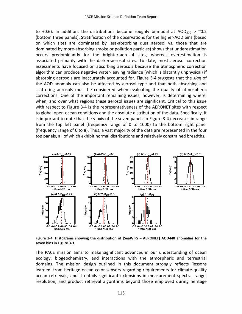
PACE Mission Science Definition Team Report
to +0.6). In addition, the distributions become roughly bi-modal at AOD870 > ~0.2 (bottom three panels). Stratification of the observations for the higher-AOD bins (based on which sites are dominated by less-absorbing dust aerosol vs. those that are dominated by more-absorbing smoke or pollution particles) shows that underestimation occurs predominantly for the brighter-aerosol sites, whereas overestimation is associated primarily with the darker-aerosol sites. To date, most aerosol correction assessments have focused on absorbing aerosols because the atmospheric correction algorithm can produce negative water-leaving radiance (which is blatantly unphysical) if absorbing aerosols are inaccurately accounted for. Figure 3-4 suggests that the sign of the AOD anomaly can also be affected by aerosol type and that both absorbing and scattering aerosols must be considered when evaluating the quality of atmospheric corrections. One of the important remaining issues, however, is determining where, when, and over what regions these aerosol issues are significant. Critical to this issue with respect to Figure 3-4 is the representativeness of the AERONET sites with respect to global open-ocean conditions and the absolute distribution of the data. Specifically, it is important to note that the y-axis of the seven panels in Figure 3-4 decreases in range from the top left panel (frequency range of 0 to 1000) to the bottom right panel (frequency range of 0 to 8). Thus, a vast majority of the data are represented in the four top panels, all of which exhibit normal distributions and relatively constrained breadths.
Figure 3-4. Histograms showing the distribution of [SeaWiFS – AERONET] AOD440 anomalies for the seven bins in Figure 3-3.
The PACE mission aims to make significant advances in our understanding of ocean ecology, biogeochemistry, and interactions with the atmospheric and terrestrial domains. The mission design outlined in this document strongly reflects ‘lessons learned’ from heritage ocean color sensors regarding requirements for climate-quality ocean retrievals, and it entails significant extensions in measurement spectral range, resolution, and product retrieval algorithms beyond those employed during heritage
115
PACE Mission Science Definition Team Report
missions. These advances will require many developments from the data analysis team and the broader science community. As part of this effort, significant work is needed to evaluate challenges associated with atmospheric corrections and determine how these challenges can be met by a close, interdisciplinary collaboration between the ocean and atmospheric science communities. Clearly, the impact of aerosol amount and type on retrieved ocean color parameters is not a straightforward problem. Addressing this issue will require model and data analyses that are far beyond the scope of the PACE SDT timeframe, but analyses should continue in earnest from this point forward and take full advantage of heritage data sets. Results of these analyses will be key in determining how much information about aerosol amount and type is needed to meet the science requirements of the PACE mission. Finally, it is important to recognize that multiple PACE ocean science retrievals are envisioned as being products of inversion algorithms that not only attempt to assess in-water absorbing components, but also particulate scattering properties. Accordingly, errors in accounting for atmospheric scattering can contribute to errors in assessed ocean properties, so attention is needed in evaluating assessments of both aerosol absorption properties and scattering properties (i.e., not just absorbing aerosols).
The ability of the PACE mission to accommodate a high-accuracy multi-directional, multi-polarization and multispectral (3M) imager would contribute significantly towards reducing any outstanding atmospheric correction errors, provided that the imager covers the same cross-track swath as the PACE ocean radiometer. Alternatively, one may consider accommodating (for this particular purpose) a single-view, multi-wavelength, high-accuracy multi-polarimetric (2M) imaging instrument with the requisite cross-track swath. A 2M instrument of this type would not achieve the enhanced aerosol objectives of the PACE mission envisioned with a 3M instrument (see Table 2-1). However, the results of a sensitivity study (see Figure 3-5) suggest that a 2M imager with high polarimetric accuracy could reduce aerosol optical depth uncertainties relative to OCI alone and potentially provide some information on aerosol absorption.
The vertical coordinates in Figure 3-5 represent the retrieval sensitivity of various aerosol parameters to measurement error (covariance matrix) for a range of atmospheric states. The retrieval state vector includes the aerosol parameters listed in Figure 3-5. The calculations are performed as in Knobelspiesse et al. [2012], i.e., they assume no forward model error sources (e.g., uncertainties caused by variations in the vertical distribution of aerosols, ocean bio-optical model, etc.). Calculations for a high-accuracy 2M and the POLDER instrument are made on the same set of state vectors from AERONET retrievals [Dubovik et al., 2002] for two maritime regions. The results can be compared as estimates of absolute retrieval uncertainty if both instruments are assumed to retrieve the same state vector across the space (not expected to be the case in general for realistic modeling uncertainties). Note that the aerosol case studies shown in Figure 3-5 are chosen to express the sensitivity at different locations in the nonlinear measurement/parameter space. That is, the results for these two cases bracket values
116
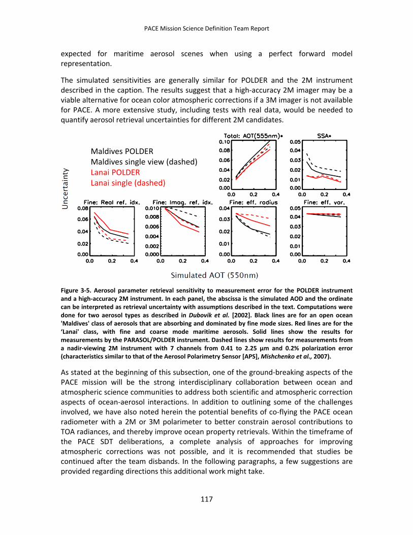
PACE Mission Science Definition Team Report
expected for maritime aerosol scenes when using a perfect forward model representation.
The simulated sensitivities are generally similar for POLDER and the 2M instrument described in the caption. The results suggest that a high-accuracy 2M imager may be a viable alternative for ocean color atmospheric corrections if a 3M imager is not available for PACE. A more extensive study, including tests with real data, would be needed to quantify aerosol retrieval uncertainties for different 2M candidates.
Maldives POLDERMaldives single view (dashed)Lanai POLDERLanai single (dashed)
Figure 3-5. Aerosol parameter retrieval sensitivity to measurement error for the POLDER instrument and a high-accuracy 2M instrument. In each panel, the abscissa is the simulated AOD and the ordinate can be interpreted as retrieval uncertainty with assumptions described in the text. Computations were done for two aerosol types as described in Dubovik et al. [2002]. Black lines are for an open ocean 'Maldives' class of aerosols that are absorbing and dominated by fine mode sizes. Red lines are for the ‘Lanai' class, with fine and coarse mode maritime aerosols. Solid lines show the results for measurements by the PARASOL/POLDER instrument. Dashed lines show results for measurements from a nadir-viewing 2M instrument with 7 channels from 0.41 to 2.25 µm and 0.2% polarization error (characteristics similar to that of the Aerosol Polarimetry Sensor [APS], Mishchenko et al., 2007).
As stated at the beginning of this subsection, one of the ground-breaking aspects of the PACE mission will be the strong interdisciplinary collaboration between ocean and atmospheric science communities to address both scientific and atmospheric correction aspects of ocean-aerosol interactions. In addition to outlining some of the challenges involved, we have also noted herein the potential benefits of co-flying the PACE ocean radiometer with a 2M or 3M polarimeter to better constrain aerosol contributions to TOA radiances, and thereby improve ocean property retrievals. Within the timeframe of the PACE SDT deliberations, a complete analysis of approaches for improving atmospheric corrections was not possible, and it is recommended that studies be continued after the team disbands. In the following paragraphs, a few suggestions are provided regarding directions this additional work might take.
117
PACE Mission Science Definition Team Report
Currently, the amount of aerosol-type information required to significantly advance atmospheric corrections is unknown. Two complementary approaches are recommended: (1) a forward calculation based on knowledge of retrieved ocean color parameter sensitivity to a range of expected atmospheric aerosol microphysics and aerosol loading conditions, and (2) an assessment of the impact that errors in derived AOD and aerosol microphysics have had on SeaWiFS and/or MODIS ocean color retrievals. Studies based on both these approaches can be realized with currently available data. It is recommended that as part of such analyses, results be evaluated in the context of their spatial and temporal extent (i.e., over what fraction of the global ocean is there a problem?) and which specific areas and times are most problematic.
An additional direction of pursuit would be execution of a model-based Observing System Simulation Experiment (OSSE). Such a simulation would provide a useful framework for numerical experimentation. Observables could be simulated from fields generated by an Earth system model, including a parameterized description of observational error characteristics. The simulated observations could be used for hypothetical sampling studies, to estimate errors in analysis or retrieval algorithms, and ultimately to help plan the design of a new observing mission. Although this type of framework has traditionally been used to assess the impact of observations on numerical weather prediction, it has much broader applicability and would be particularly relevant to observation of aerosols and chemical constituents. We recommend such OSSEs be performed early in the PACE planning cycle. The model could include radiatively coupled aerosols and be run at a resolution of at least 10 km globally. At such high spatial resolution, global models are now capable of simulating realistic cloud and aerosol systems on a global scale. Using climatological surface characteristics derived from EOS sensors, these simulations could use a comprehensive atmospheric and oceanic vector radiative transfer model to produce simulated top-of-the atmosphere reflectances, as would be observed by the PACE ocean radiometer. In a close partnership between instrument and retrieval teams, parameterized observation errors could be added to these reflectances. These simulations will help guide the development of retrieval and data assimilation algorithms, in addition to sampling and trade-off studies during Phase A of the mission lifecycle. In particular, these OSSEs would be useful to assess the impact of PACE measurements on cloud and aerosol forecast skills, as well as to assess the effectiveness of atmospheric correction schemes.
3.3 PACE Atmosphere Measurement Requirements The PACE Ocean Ecology and Biogeochemistry team provides OCI imager measurement requirements for retrieving ocean geophysical parameters in section 3.2. Here the PACE Atmosphere Team discusses additional OCI capabilities needed for continuing a subset of cloud data records and/or aerosol data records as described in sections 2.3.1 and 2.3.2.
118
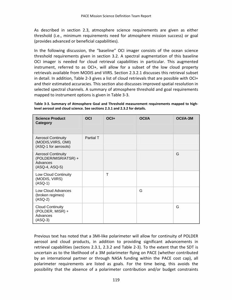
PACE Mission Science Definition Team Report
As described in section 2.3, atmosphere science requirements are given as either threshold (i.e., minimum requirements need for atmosphere mission success) or goal (provides advanced or beneficial capabilities).
In the following discussion, the “baseline” OCI imager consists of the ocean science threshold requirements given in section 3.2. A spectral augmentation of this baseline OCI imager is needed for cloud retrieval capabilities in particular. This augmented instrument, referred to as OCI+, will allow for a subset of the low cloud property retrievals available from MODIS and VIIRS. Section 2.3.2.1 discusses this retrieval subset in detail. In addition, Table 2-3 gives a list of cloud retrievals that are possible with OCI+ and their estimated accuracies. This section also discusses improved spatial resolution in selected spectral channels. A summary of atmosphere threshold and goal requirements mapped to instrument options is given in Table 3-3.
Table 3-3. Summary of Atmosphere Goal and Threshold measurement requirements mapped to high-level aerosol and cloud science. See sections 2.3.1 and 2.3.2 for details.
Science Product Category
OCI OCI+
OCI/A OCI/A-3M
Aerosol Continuity (MODIS,VIIRS, OMI) (ASQ-1 for aerosols)
Partial T
Aerosol Continuity (POLDER/MISR/ATSR) + Advances (ASQ-4, ASQ-5)
G
Low Cloud Continuity (MODIS, VIIRS) (ASQ-1)
T
Low Cloud Advances (broken regimes) (ASQ-2)
G
Cloud Continuity (POLDER, MISR) + Advances (ASQ-3)
G
Previous text has noted that a 3MI-like polarimeter will allow for continuity of POLDER aerosol and cloud products, in addition to providing significant advancements in retrieval capabilities (sections 2.3.1, 2.3.2 and Table 2-3). To the extent that the SDT is uncertain as to the likelihood of a 3M polarimeter flying on PACE (whether contributed by an international partner or through NASA funding within the PACE cost cap), all polarimeter requirements are listed as goals. For the time being, this avoids the possibility that the absence of a polarimeter contribution and/or budget constraints
119
PACE Mission Science Definition Team Report
result in a mission that cannot meet minimum success criteria. That said, it is imperative that evolving international partnerships and budget realities be folded into ongoing PACE polarimeter discussions with the SDT or a similar mission science team body as appropriate.
Following the same organization as section 3.2, atmosphere requirements are sub-divided into ten categories (e.g., global coverage, etc.). Ocean color requirements either exceed or are equivalent to aerosol and cloud requirements for many of the categories.
3.3.1 Orbit Threshold requirement: As for section 3.2 ocean color requirements, specifically a polar orbit with an equatorial crossing time between 1100 and 1300 local time (LT), maintained to ±10 minutes over the lifetime of the mission.
Goal: A polar orbit with an equatorial crossing time of 1330 LT allowing some coincident overlap with the JPSS-1 orbit (nominally at 1330 LT, ~825 km altitude) and providing time-of-day continuity with MODIS Aqua and A-Train observations.
3.3.2 Spatial and Temporal Coverage Same as section 3.2, except specification of solar zenith angle range of data collection as follows:
Solar zenith angle range of data collection:
• Threshold requirement: ≤ 81.5° (cosine of solar zenith angle ≥ 0.15) for continuity with L2 products from MODIS/VIIRS and imagery that provides cloud and meteorological context for nearby ocean retrievals having smaller solar zenith angle constraints.
• Goal: > 81.5°.
3.3.3 Navigation and Registration Same as section 3.2.
3.3.4 Instrument Performance Tracking Same as section 3.2.
120
PACE Mission Science Definition Team Report
3.3.5 Instrument Artifacts Same as section 3.2.
3.3.6 Spatial Resolution Same as section 3.2, except goal requirements as follows:
• Sample size goal: 250 m spatial resolution at suborbital track 20° tilt angle for selected OCI channels (see Table 3-4).
• Along-track sample spacing goal: 250 m in selected channels at suborbital track (see Table 3-4).
Appendix B provides further details regarding the rationale for higher spatial resolution than the baseline 1 km specification (reduction of low cloud heterogeneity biases).
3.3.7 Atmospheric Corrections Not applicable (no distinction is made between science spectral bands and those bands used for supplementary purposes). Though extinction/correction for various atmospheric constituents is needed for aerosol and cloud retrievals, these capabilities are inclusive of requirements given elsewhere in this section.
3.3.8 Aerosol and Cloud Science Spectral Bands Same as section 3.2, except:
1. Addition of three spectral channels as goal requirements. These are given in Table 3-4 (nominal center wavelength at 0.94, 1.38, and 2.25 µm).
Section 2.3.2 provided the basic rationale for the inclusion of these channels. To summarize, they include: (a) 1.38 µm thin cirrus detection/masking for aerosol retrievals, continuity with MODIS cloud detection [Ackerman et al., 2008], and cirrus optical thickness retrievals [Meyer and Platnick, 2012]; (b) 0.94 µm water vapor channel combined with synergistic O2 A-band observations for diagnosing multilayer scenes [Wind et al., 2010; Lindstrot et al., 2010]; and (c) 2.25 µm channel for continuity with VIIRS and future GOES-R ABI cloud microphysical observations, and improved cloud thermodynamic phase information [Pilewskie and Twomey, 1987; Zinner et al., 2008, Martins et al., 2011]. Appendix B provides further details regarding items (b) and (c).
2. Explicit specifications on an O2 A-band capability expected to be part of the baseline OCI imager (see Table 3-4).
121
PACE Mission Science Definition Team Report
3.3.9 Signal-to-noise Same as section 3.2, except for augmented atmospheric channels as given in Table 3-4.
3.3.10 Data Processing, Reprocessing, and Distribution Same as section 3.2 (capability for semi-annual data reprocessing), except for the addition of a latency requirement for aerosol/cloud data assimilation and application purposes.
The NASA Land and Atmosphere Near real-time Capability for EOS (LANCE) system (http://earthdata.nasa.gov/data/near-real-time-data) currently provides 3-hour data latency that is adequate for current community needs. This fits well with a 6-hour data assimilation frequency (at 0, 6, 12 and 18 Coordinated Universal Time [UTC]). By 2020 it is conceivable that this frequency will be reduced to 3 hours (implying a 1.5-hour data latency requirement). However, while shorter latencies for cloud-masked radiances will be needed in the future, less stringent latencies for Level 2 products may be acceptable as data assimilation systems eventually move towards radiance assimilation for aerosols and clouds.
• Data latency threshold requirement: 3-hour data latency for the distribution of preliminary L1B data with cloud masking, as well as a 3-hour latency for Level 2 aerosol and cloud products.
• Data latency goal: 1.5-hour latency for cloud-masked radiances, with 3-hour latency for Level 2 aerosol and cloud products.
3.3.11 Summary of Cloud and Aerosol Augmentations to the Baseline OCI Imager
Table 3-4 below summarizes the cloud and aerosol augmentations to the baseline OCI imager specifications.
122
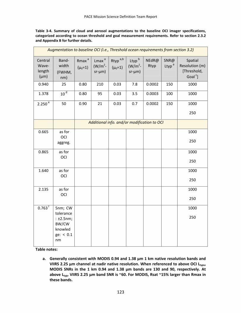
PACE Mission Science Definition Team Report
Table 3-4. Summary of cloud and aerosol augmentations to the baseline OCI imager specifications, categorized according to ocean threshold and goal measurement requirements. Refer to section 2.3.2 and Appendix B for further details.
Augmentation to baseline OCI (i.e., Threshold ocean requirements from section 3.2)
Central Wave-length (µm)
Band-width
(FWHM, nm)
Rmax a (µ0=1)
Lmax a (W/m2-sr-µm)
Rtyp a,b (µ0=1)
Ltyp b (W/m2-sr-µm)
NEdR@Rtyp
SNR@Ltyp a
Spatial Resolution (m)
[Threshold, Goal c]
0.940 25 0.80 210 0.03 7.8 0.0002 150 1000
1.378 10 d 0.80 95 0.03 3.5 0.0003 100 1000
2.250 e 50 0.90 21 0.03 0.7 0.0002 150 1000
250
Additional info. and/or modification to OCI
0.665 as for OCI
aggreg.
1000
250
0.865 as for OCI
1000
250
1.640 as for OCI
1000
250
2.135 as for OCI
1000
250
0.763 f 5nm; CW tolerance: ±2.5nm; BW/CW knowledge: < 0.1 nm
1000
250
Table notes:
a. Generally consistent with MODIS 0.94 and 1.38 µm 1 km native resolution bands and VIIRS 2.25 µm channel at nadir native resolution. When referenced to above OCI Ltyps, MODIS SNRs in the 1 km 0.94 and 1.38 µm bands are 130 and 90, respectively. At above Ltyp, VIIRS 2.25 µm band SNR is ~60. For MODIS, Rsat ~15% larger than Rmax in these bands.
123
PACE Mission Science Definition Team Report
b. Rtyp corresponds to cirrus optical thickness of approximately 0.2–0.3.
c. Goal spatial resolution for reduction of low cloud heterogeneity biases.
d. Goal BW (MODIS 30 nm BW found to be too large for adequate cirrus detection; VIIRS 15 nm found to be significantly better).
e. For cloud phase and VIIRS/ABI cloud microphysics continuity.
f. POLDER and Medium-spectral Resolution Imaging Spectrometer (MERIS) cloud pressure height heritage.
3.4 Terrestrial Ecology The following goal requirements that would provide advanced or beneficial capabilities for observations of terrestrial ecosystems are suggested:
1) The spectrometer wavelength range should be extended to at least 800 nm. This extension will fully describe the terrestrial vegetation “red edge,” which is critical for observing foliage chlorophyll concentrations.
2) A SWIR band at 1375 nm (1360–1390 nm) should be added to detect cirrus clouds.
3) Due to the spatial heterogeneity of landscapes, pixel sizes between 250 and 500 m are preferable [Townshend and Justice, 1988]. If all bands cannot be provided at this finer resolution, selected wavelengths would be useful. Suggested fine resolution bands are at 0.665, 0.865, and 1.640 µm. The first two bands can be used to calculate the Normalized Difference Vegetation Index (NDVI), a measure of amounts of green vegetation, and the last two bands can calculate the Normalized Difference Infrared Index (NDII), a measure of vegetation water content.
124
PACE Mission Science Definition Team Report
4 PACE Spacecraft and Mission Support Requirements
4.1 Introduction The PACE instrument suite will be operated from a sun-synchronous polar orbit on a dedicated spacecraft bus. To achieve the stated science objectives, a thorough instrument calibration strategy will be needed to monitor and maintain radiometric performance over the mission lifespan. This strategy must be coupled with a comprehensive program for vicarious calibration, geophysical product validation, and algorithm development that relies heavily on ground-based measurements of ocean biogeochemical properties and oceanic and atmospheric optical properties. A dedicated field program is thus a mission requirement, as is a capable data system scaled to process, archive, and distribute the large data volumes anticipated from PACE, and to reprocess data as instrument calibration knowledge evolves and advanced algorithms are developed. To produce a time series of sufficient quality for climate research, the instrument and vicarious calibration, algorithm implementation, product validation, and data reprocessing must be closely coordinated, and thus we strongly recommend the establishment of an integrated data support team (IDST) to perform these core functions for the PACE mission. Requirements for spacecraft, instrument operations and scheduling, post-launch instrument calibration, field program support, and data systems are detailed in the sections that follow.
4.2 Launch Vehicle A NASA-certified medium-class launch vehicle (LV) suitable for the PACE mission will be selected roughly 30 months before the scheduled launch date. Currently, NASA’s published acquisition strategy assumes that affordable LVs developed for International Space Station (ISS) resupply missions will be available through the Commercial Orbital Transportation Services (COTS) Program within a few years—well before the PACE LV acquisition date. However, at the time of this writing, NASA has not certified any of the ISS resupply LVs for science missions, opening up the possibility of appreciable cost and schedule risk in the PACE mission, if a suitable medium-class launch vehicle is not certified by NASA before 2016. Candidate medium-class LVs suitable for PACE include: Athena IIIA, Delta II, Evolved Expendable Launch Vehicle (EELV), Antares, Falcon 9 and Minotaur IV.
4.3 Spacecraft Requirements The PACE mission will require a spacecraft with sufficient resources and operating conditions to support the science instrument suite in the collection, storage, and transmission to the surface of Earth spectral radiance measurements and science and engineering telemetry. In addition, the spacecraft provides the mechanical interface
125
PACE Mission Science Definition Team Report
with the launch vehicle, including the structural and material characteristics needed to package and launch the science payload and other payload elements efficiently and safely into low Earth orbit. Requirements for this bus are driven by size, mass, power, and downlink data rate of the science instrument(s). In addition, special requirements of the PACE mission related to clear fields of view and system-level pointing stability and knowledge, and radiometric calibration-related requirements for scanning all detectors in the spectroradiometer—both across the Earth and across the moon once or twice a month—impact detailed specifications for the PACE spacecraft. The PACE mission requirement for tilting the instrument to avoid sun glint is also an important specified spacecraft capability. The discussion presented here is intended only to capture PACE-specific requirements and notional instrument characteristics that are expected to constrain the spacecraft design. The discussion purposefully does not describe specific or possible spacecraft design approaches. Details of the spacecraft specification will depend on the science payload design that is ultimately selected for PACE. The eventual design may differ from approaches studied in the NASA Goddard PACE Instrument Design Laboratory (IDL) engineering studies completed in conjunction with this SDT report (available at http://decadal.gsfc.nasa.gov/pace.html). The Ocean Color Experiment-2 (OCE2) IDL study was driven by the ocean mission threshold requirements, and the OCE3 IDL study was driven by ocean mission goals and uses a different design approach than OCE2. The PACE SDT encourages potential instrument suppliers to offer instrument designs with reduced size, mass, power, and data rate relative to the OCE2 and OCE3 notional designs, while meeting all threshold mission requirements and possibly addressing goal requirements. Similarly, some spacecraft requirements may differ from the notional characteristics presented here as determined by agreements among NASA, the spacecraft provider and the instrument provider. The notional characteristics presented here are generally consistent with characteristics of spacecraft available through the NASA Goddard Space Flight Center (GSFC) Rapid Spacecraft Development Office (RSDO) Catalog.
A nominal orbit for PACE is a 705-km sun-synchronous orbit with an inclination of 98 degrees and a noon Local Time equatorial crossing of the Ascending Node (LTAN), which would satisfy the ocean ecology and biogeochemistry requirements described in section 3.2 and meet the threshold requirements for atmospheric science described in section 3.3. The PACE mission requirement to cover the entire Earth every two days leads to a maximum cross-track viewing angle of 51 degrees off nadir from 705 km altitude, which helps define the size of the minimum clear field of view that must be provided by the spacecraft. Similarly, in the fore and aft directions, clear field of view provided by the spacecraft is driven in part by the mission requirement for the instrument to be able to avoid sun glint by tilting its line of sight in the fore and aft directions by up to 20 degrees off nadir. It is conceivable that this tilting function could be allocated to the spacecraft rather than the instrument, although the need to complete the full 40 degree tilt motion in 15 seconds or less is expected to be a challenging requirement for a spacecraft.
126
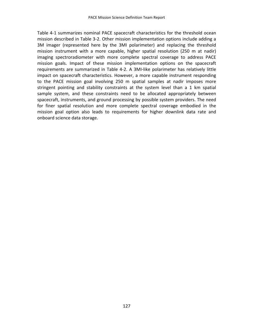
PACE Mission Science Definition Team Report
Table 4-1 summarizes nominal PACE spacecraft characteristics for the threshold ocean mission described in Table 3-2. Other mission implementation options include adding a 3M imager (represented here by the 3MI polarimeter) and replacing the threshold mission instrument with a more capable, higher spatial resolution (250 m at nadir) imaging spectroradiometer with more complete spectral coverage to address PACE mission goals. Impact of these mission implementation options on the spacecraft requirements are summarized in Table 4-2. A 3MI-like polarimeter has relatively little impact on spacecraft characteristics. However, a more capable instrument responding to the PACE mission goal involving 250 m spatial samples at nadir imposes more stringent pointing and stability constraints at the system level than a 1 km spatial sample system, and these constraints need to be allocated appropriately between spacecraft, instruments, and ground processing by possible system providers. The need for finer spatial resolution and more complete spectral coverage embodied in the mission goal option also leads to requirements for higher downlink data rate and onboard science data storage.
127
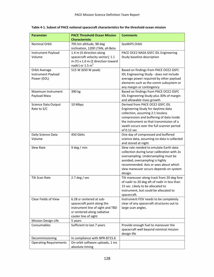
PACE Mission Science Definition Team Report
Table 4-1. Subset of PACE notional spacecraft characteristics for the threshold ocean mission
Parameter PACE Threshold Ocean Mission Characteristic
Comments
Nominal Orbit 705 km altitude, 98 deg inclination, 1200 LTAN, all-Beta
SeaWiFS Orbit
Instrument Payload Volume
1.4 m (X direction along spacecraft velocity vector); 1.1 m (Y) x 1.0 m (Z direction toward nadir) or 1.5 m3
PACE OCE2 NASA GSFC IDL Engineering Study baseline description
Orbit Average Instrument Payload Power (EOL)
515 W (650 W peak) Based on findings from PACE OCE2 GSFC IDL Engineering Study - does not include average power required by other payload elements such as the comm subsystem or any margin or contingency
Maximum Instrument Payload Mass
390 kg Based on findings from PACE OCE2 GSFC IDL Engineering Study plus 30% of margin and allowable mass growth
Science Data Output Rate to S/C
10 Mbps Derived from PACE OCE2 GSFC IDL Engineering Study for daytime data collection, assuming 2:1 lossless compression and buffering of data inside the instrument so that transmission of a swath occurs over the full scanner period of 0.12 sec
Daily Science Data Volume
450 Gbits One day of compressed and buffered science data, assuming no data is collected and stored at night
Slew Rate 9 deg / min Slew rate needed to emulate Earth data collection during lunar calibration with 2x oversampling. Undersampling must be avoided; oversampling is highly recommended. Axis or axes about which slew maneuver occurs depends on system design.
Tilt Scan Rate 2.7 deg / sec Tilt maneuver along track from 20 deg fore of nadir to 20 deg aft of nadir in less than 15 sec. Likely to be allocated to instrument, but could be allocated to spacecraft.
Clear Fields of View 6.28 sr centered at sub-spacecraft point along the instrument line of sight and TBD sr centered along radiative cooler line of sight
Instrument FOV needs to be completely clear of any spacecraft structures out to large scan angles.
Mission Design Life 5 years Consumables Sufficient to last 7 years Provide enough fuel to maneuver the
spacecraft well beyond nominal mission design life
Decommissioning In compliance with NPR-8715.6 Operating Requirements On-orbit software uploads, 1 ms
absolute timing
128
PACE Mission Science Definition Team Report
Parameter PACE Threshold Ocean Mission Characteristic
Comments
Thermal Radiator on anti-sun side of spacecraft; no heat exchanged between instrument and spacecraft
Heat exchanged between instrument and spacecraft may be negotiated between instrument and spacecraft suppliers
Contamination Spacecraft materials and bakeout plan compatible with UV Instrument Class Contamination Control Plan
Ultraviolet optics used in PACE are especially sensitive to degradation resulting from particulate and outgassing contamination
Compatible Launch Vehicles (LVs)
Antares, Atlas V, Athena IIIA, Delta II, Delta IV, Falcon 9, Minotaur IV
Medium class LV candidates for PACE available in 2012 - LV selection depends on cost and schedule constraints along with NASA LV certifications currently in process
Table 4-2. Changes in PACE notional spacecraft =characteristics resulting from other mission options
Changes in Spacecraft Characteristics with Respect to PACE Ocean Mission Threshold Resulting from Mission Options
Parameter 3MI-like Polarimeter (representative of possible ADDITION to PACE Threshold Ocean Mission System [values in Table 4-1] or to Ocean Mission Goal System [values in column to the right])
PACE Ocean Mission Goal System (250 m and 1000 m spatial samples at nadir depending on spectral band with more complete spectral coverage than OCE2) as described in PACE OCE3 GSFC IDL Study - REPLACES PACE Ocean Mission Threshold System as described in PACE OCE2 NASA GSFC IDL Engineering Study and Table 4-1
Instrument Payload Volume 0.8 m (X); 0.7 m (Y) x 0.5 m (Z) or 0.3 m3
1.3 m (X); 1.7 m (Y) x 1.0 m (Z) or 2.2 m3
Orbit Average Instrument Payload Power (EOL)
85 W (100 W peak) 390 W (500 W peak)
Maximum Instrument Payload Mass
60 kg (no margin or allowable mass growth)
360 kg (includes 30% margin and allowable mass growth)
Science Data Output Rate to S/C 2.2 Mbps (assuming 3:1 compression ratio)
125 Mbps
Daily Science Data Volume 114 Gbits 5.4 Tbits
4.4 Onboard Calibration Requirements This section discusses the onboard calibration requirements that were formulated in section 3.2 for the PACE ocean radiometer:
129
PACE Mission Science Definition Team Report
1) Long term degradation monitoring (monthly measurements of the sensor gain factor(s) with an accuracy of +/-0.2% (goal: +/-0.1%)
2) Daily observations of a calibration target with an accuracy of ~0.2%
3) Monthly characterization of instrument spectral drift with an accuracy of 0.3 nm
The main purpose of this section is to discuss the implementation of these requirements based on the experience with heritage sensors.
The most challenging of the calibration requirements is the long term degradation monitoring. The ambitious requirement of +/-0.2% accuracy requires at least two independent methods to track the radiometric degradation. At least one of the two methods should use lunar measurements with an optical path in the instrument identical to the one used for regular Earth-viewing measurements to ensure full applicability to the ocean products. Neither method should rely on assumptions about the Earth’s atmosphere or ground surface reflectance to avoid influencing the degradation trending by geophysical changes.
4.4.1 Long-term Degradation Monitoring Degradation trending of radiometric sensitivity is the most important aspect of on-orbit sensor calibration and characterization activities. The ocean color community recognizes that lunar measurements have a superior track record [e.g. IOCCG, 2012]. The long-term stability that has been achieved with this methodology for the SeaWiFS mission lifetime is on the order of 0.1% [Eplee et al., 2011].
The two main advantages of lunar measurements are that (1) there is no atmosphere in the optical path, removing a large potential source of uncertainty, and (2) lunar reflectance is constant over geological time scales [Kieffer, 1997], surpassing any reasonable radiometric accuracy requirements.
Although the lunar reflectance is constant, the lunar irradiance as seen from Earth varies considerably, even for a constant lunar phase angle (a lunar phase angle of 0° corresponds to full moon, 90° to new moon; note that the irradiance from a new moon is essentially 0). These variations are predictable and depend mainly on the moon-sun and Earth-moon distances, and on libration (slight variations of the orientation of the moon relative to the Earth). The U.S. Geological Survey Robotic Lunar Observatory (ROLO) model predicts these variations. The ROLO model was derived from a multiyear measurement campaign of lunar irradiances using an Earth-based radiometer [Kieffer and Stone, 2005]. To use the moon as a calibration source, each detector in the PACE ocean color radiometer must acquire an image of the entire moon, to enable tying the measurements to the ROLO spectral irradiance model.
130
PACE Mission Science Definition Team Report
Note that lunar irradiances provided by the ROLO model are known to contain a relatively large bias. Nevertheless, the precision of the lunar irradiances provided by the ROLO model is excellent. Therefore, lunar measurements are ideal (depending on instrument type, see below) for relative temporal gain trending, but not the first choice for absolute calibration accuracy. At the time of this writing, efforts are in the early planning stages at the National Institute of Standards and Technology (NIST) to develop a lunar measurement campaign that may allow significant improvements to the absolute accuracy of the ROLO model.
Challenges associated with using the moon as a calibration source include:
1) Lunar irradiance variations: Lunar irradiance measured from an Earth-orbiting sensor depends strongly on several factors, such as the Earth-sun distance, moon-sun distance, libration, and lunar phase angle. These variations are captured by the ROLO model. By acquiring lunar measurements at a constant phase angle, a long-term trending accuracy of 0.1% can be achieved [Stone and Kieffer, 2004]. Therefore, lunar irradiance variations are a manageable issue.
2) Spatial radiance variations: Lunar reflectance has strong spatial variation, as evidenced by the dark maria and bright highlands that are readily visible to human observers. For a typical Earth-observing sensor with 1 km resolution, these brightness variations are resolved in the acquired image, as shown in Figure 4-1. The ROLO model provides only the lunar irradiance (i.e., the sum of radiances over all lunar pixels); it cannot provide the radiances for individual pixels. Although a lunar radiance model for individual pixels is under development, the expected precision is at best about 5.0% for individual measurements, and 0.5% for long-term precision [T. Stone, private communication]. This is an issue for sensors like MODIS, because these sensors measure the lunar image with multiple detectors. MODIS uses up to 10 detectors for its 1 km resolution bands. Only one calibration factor per band and mirror side is derived for the operational MODIS calibration. Note that a) MODIS uses lunar measurements only as a detector-independent adjustment to the scan-angle dependence of the radiometric sensitivity [Sun et al., 2007], and b) it is possible to derive one calibration factor per detector for the MODIS 1 km bands, but the uncertainties are much larger [Sun et al., 2007]. To summarize, the spatial radiance variations of the lunar surface severely complicate the calibration effort, unless each sensor element (e.g., each detector) that needs to be calibrated acquires a complete image of the lunar disk to allow a comparison to the irradiance provided by the ROLO model.
3) Calibration frequency: Lunar irradiance varies strongly with phase angle. To optimize the long-term trending accuracy, phase angle should be kept constant, which means that lunar calibration measurements can be performed only once every lunar month (29.5 days). If measurements are scheduled at the same absolute value of phase angle before and after full moon, two lunar calibrations
131
PACE Mission Science Definition Team Report
per month are possible, leading to a potential increase in precision. This would be especially helpful at the beginning of the mission (trending precision is usually worst at the beginning and end of a time series). Although the intervals of once or twice per month are sufficient for long-term trending, a separate calibration mechanism (e.g., a solar diffuser) is needed to resolve short-term variations of radiometric sensitivity of the sensor.
4) Optimal phase angle: The choice of phase angle involves at least two considerations. The first is the larger the phase angle, the fewer the number of useful lunar pixels available for the irradiance calculation. Therefore, a larger phase angle is expected to decrease the precision of the irradiances measured by the sensor, although this has not been quantified. The second consideration is that at very small phase angles, lunar backscatter decreases the accuracy of the ROLO model [Stone et al., 2004]. For the SeaWiFS sensor, a phase angle of 7° was chosen, leading to excellent results. The ROLO model uncertainty of 1% for each measurement is valid for phase angles larger than 7°, but the ROLO model uncertainty for long-term measurements of 0.1% has only been demonstrated for the SeaWiFS phase angle. Therefore, a 7° phase angle should be targeted for the PACE lunar calibrations. Preferably, the phase angle should be always at either a waxing or waning moon (no preference for either one) to avoid switching phase angle between calibrations. For different target phase angles, long-term precision implications must be analyzed. Note that lunar phase increases by about 0.85° per orbit. Limiting the range of phase angles to 6.5° to 7.5°, for example, will allow one measurement in this range per lunar month (or two for both waxing and waning moon). If there are additional operational constraints that do not allow this range of phase angles, the phase angle range should be extended to 6.0° to 8.0°.
5) Additional phase angles: Increasing the frequency of lunar measurements is expected to increase precision of the trending of radiometric degradation of the sensor. The amount of this increase is speculative at the moment. The SeaWiFS precision was achieved with only one measurement per month. Possible advantages of additional phase angles have to be weighed against the increased resources needed to obtain the additional measurements (e.g., the power needed to maneuver the instrument into a position where it can see the moon). An obvious choice for increasing the number of lunar measurements beyond a single measurement would be to calibrate at both 7° before and after full moon, as discussed above.
132
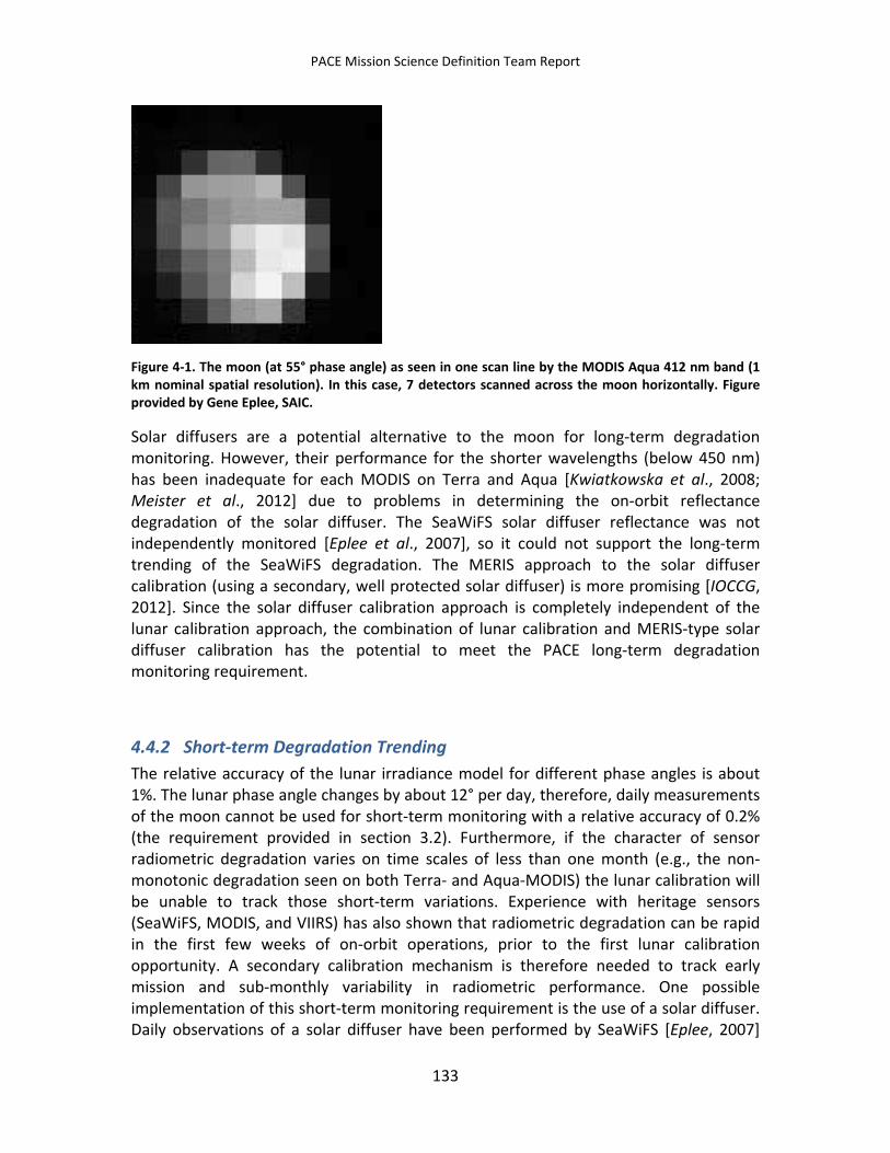
PACE Mission Science Definition Team Report
Figure 4-1. The moon (at 55° phase angle) as seen in one scan line by the MODIS Aqua 412 nm band (1 km nominal spatial resolution). In this case, 7 detectors scanned across the moon horizontally. Figure provided by Gene Eplee, SAIC.
Solar diffusers are a potential alternative to the moon for long-term degradation monitoring. However, their performance for the shorter wavelengths (below 450 nm) has been inadequate for each MODIS on Terra and Aqua [Kwiatkowska et al., 2008; Meister et al., 2012] due to problems in determining the on-orbit reflectance degradation of the solar diffuser. The SeaWiFS solar diffuser reflectance was not independently monitored [Eplee et al., 2007], so it could not support the long-term trending of the SeaWiFS degradation. The MERIS approach to the solar diffuser calibration (using a secondary, well protected solar diffuser) is more promising [IOCCG, 2012]. Since the solar diffuser calibration approach is completely independent of the lunar calibration approach, the combination of lunar calibration and MERIS-type solar diffuser calibration has the potential to meet the PACE long-term degradation monitoring requirement.
4.4.2 Short-term Degradation Trending The relative accuracy of the lunar irradiance model for different phase angles is about 1%. The lunar phase angle changes by about 12° per day, therefore, daily measurements of the moon cannot be used for short-term monitoring with a relative accuracy of 0.2% (the requirement provided in section 3.2). Furthermore, if the character of sensor radiometric degradation varies on time scales of less than one month (e.g., the non-monotonic degradation seen on both Terra- and Aqua-MODIS) the lunar calibration will be unable to track those short-term variations. Experience with heritage sensors (SeaWiFS, MODIS, and VIIRS) has also shown that radiometric degradation can be rapid in the first few weeks of on-orbit operations, prior to the first lunar calibration opportunity. A secondary calibration mechanism is therefore needed to track early mission and sub-monthly variability in radiometric performance. One possible implementation of this short-term monitoring requirement is the use of a solar diffuser. Daily observations of a solar diffuser have been performed by SeaWiFS [Eplee, 2007]
133
PACE Mission Science Definition Team Report
and VIIRS. For the VIIRS, MODIS and MERIS sensors, the solar diffuser calibration approach was augmented by special devices to monitor the degradation of the reflectance of the solar diffuser (a separate radiometer for MODIS [Sun et al., 2005] and VIIRS, a separate, less frequently illuminated [only every 3 months] diffuser for MERIS [Delwart et al., 2009]).
4.4.3 Spectral Monitoring Most of the heritage ocean color sensors are filter radiometers, i.e., spectral bandpass filters determine which wavelengths reach the detectors. For most sensors, no on-orbit monitoring was performed; it was assumed that the filter characteristics did not change on-orbit. An independent calibration device was installed with the MODIS sensors on the Aqua and Terra missions—the Spectroradiometric Calibration Assembly (SRCA). The SRCA can monitor the spectral characteristics of MODIS; e.g., it determined that except for band 8 (412 nm), the center wavelengths of the MODIS Terra bands shifted less than 0.5 nm relative to the prelaunch characterization, and on-orbit shifts were less than 0.2 nm on average in 5 years [Xiong et al., 2006].
For hyperspectral radiometers, monitoring the wavelength characteristics of the sensor is even more important. The MERIS sensor uses a spectrally doped diffuser, solar Fraunhofer lines, and the oxygen O2A band to monitor on-orbit spectral drifts [Delwart et al., 2007]. The accuracy of the doped diffuser spectral characterization was on the order of 1 nm; the latter two methods agreed to within better than 0.1 nm. (Note that the latter two methods only cover a limited part of the spectral range).
Any instrument proposed for the PACE mission should provide a well defined strategy to track the spectral characteristics of the sensor on-orbit. The MERIS approach provided excellent results at relatively little cost.
4.4.4 Spatial Monitoring The areas sampled by two different bands for a single pixel may not overlap by 100%. This issue is referred to as band coregistration (or band-to-band registration). There are several ways of monitoring band coregistration on-orbit. Lunar measurements can be used because of the sharp edge of the lunar disk [Sun et al., 2005]. The SRCA mentioned in the previous section is routinely used in both MODIS instruments to analyze band coregistration [Xiong et al., 2005].
Geolocating a pixel refers to the determination of the geographic coordinates of the center of the area of the pixel. Accurate spacecraft attitude information is needed. In the case of MODIS, a network of ground-control points is used to increase the geolocation accuracy to approximately 50 m at nadir [Wolfe et al., 2002], and trends are monitored continuously.
134
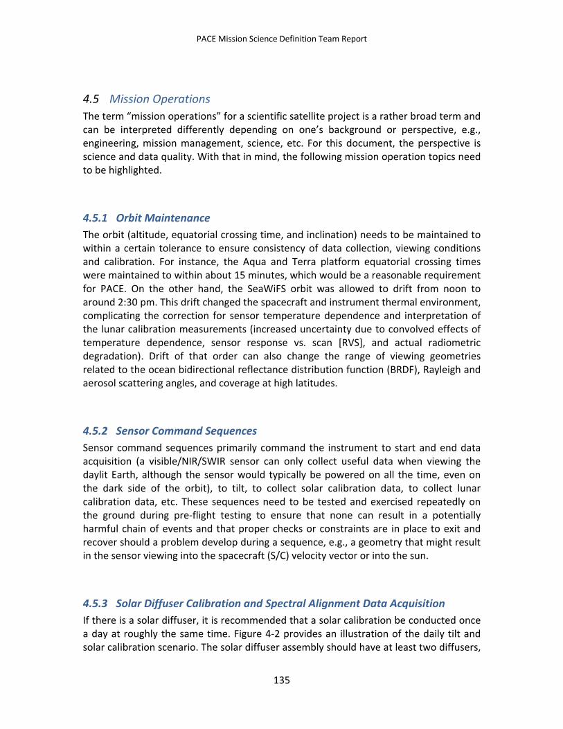
PACE Mission Science Definition Team Report
4.5 Mission Operations The term “mission operations” for a scientific satellite project is a rather broad term and can be interpreted differently depending on one’s background or perspective, e.g., engineering, mission management, science, etc. For this document, the perspective is science and data quality. With that in mind, the following mission operation topics need to be highlighted.
4.5.1 Orbit Maintenance The orbit (altitude, equatorial crossing time, and inclination) needs to be maintained to within a certain tolerance to ensure consistency of data collection, viewing conditions and calibration. For instance, the Aqua and Terra platform equatorial crossing times were maintained to within about 15 minutes, which would be a reasonable requirement for PACE. On the other hand, the SeaWiFS orbit was allowed to drift from noon to around 2:30 pm. This drift changed the spacecraft and instrument thermal environment, complicating the correction for sensor temperature dependence and interpretation of the lunar calibration measurements (increased uncertainty due to convolved effects of temperature dependence, sensor response vs. scan [RVS], and actual radiometric degradation). Drift of that order can also change the range of viewing geometries related to the ocean bidirectional reflectance distribution function (BRDF), Rayleigh and aerosol scattering angles, and coverage at high latitudes.
4.5.2 Sensor Command Sequences Sensor command sequences primarily command the instrument to start and end data acquisition (a visible/NIR/SWIR sensor can only collect useful data when viewing the daylit Earth, although the sensor would typically be powered on all the time, even on the dark side of the orbit), to tilt, to collect solar calibration data, to collect lunar calibration data, etc. These sequences need to be tested and exercised repeatedly on the ground during pre-flight testing to ensure that none can result in a potentially harmful chain of events and that proper checks or constraints are in place to exit and recover should a problem develop during a sequence, e.g., a geometry that might result in the sensor viewing into the spacecraft (S/C) velocity vector or into the sun.
4.5.3 Solar Diffuser Calibration and Spectral Alignment Data Acquisition If there is a solar diffuser, it is recommended that a solar calibration be conducted once a day at roughly the same time. Figure 4-2 provides an illustration of the daily tilt and solar calibration scenario. The solar diffuser assembly should have at least two diffusers,
135
PACE Mission Science Definition Team Report
one used each day and another used much more conservatively to preserve its stability, e.g., quarterly. This strategy has been successfully demonstrated by MERIS and presumably eliminates the need for a solar diffuser stability monitor. The assembly could also have a separate doped reflector that would be viewed at some regularity, e.g., monthly, to track spectral stability, which would be needed for a dispersive optical design like a grating or prism.
Figure 4-2. A depiction of the sensor tilt and solar calibration scenarios for a descending (north to south) orbit.
4.5.4 Lunar Data Acquisition (Monthly) As a result of the successful use of the moon for monitoring the SeaWiFS relative calibration stability, a lunar calibration is recommended for PACE. In the case of SeaWiFS, the S/C was allowed to pitch 360° such that the sensor imaged the moon through the Earth-view aperture. The maneuver is handled in the flight software, which controls when and at what rate the pitch is executed. This activity also requires a scheduled data acquisition during the lunar view.
136
PACE Mission Science Definition Team Report
4.5.5 Sensor Tilt Sequences (Each Orbit) The tilt change is designed to reduce sun glint contamination, greatly improving coverage and data quality. In Figure 4-2, the S/C is moving from north to south on the sunlit side of the orbit. Initially, the sensor is tilted away from the sun, looking aft. As the orbit approaches the subsolar point, the sensor is tilted forward so as to continue viewing away from the sun. This tilt change needs to be staggered somewhat orbit-to-orbit to avoid a band of no data collection at the subsolar point. The gaps are filled by off-nadir data from adjacent orbits. This strategy was successfully demonstrated by SeaWiFS. Note that for the solar diffuser data collection (once/day), the sensor may need to be commanded to a specific tilt depending on the diffuser geometry.
4.5.6 Data Downlink Scheduling (Each Orbit) Given the large data volumes anticipated from the PACE sensor(s) and the fact that the ground contact time averages about 10 minutes per orbit for high latitude stations, accurate scheduling of time and duration for multiple data downlinks per day (possibly every orbit) will be required. Also, accommodations for additional downlinks may be necessary in case some downlinks are missed due to ground station problems, etc. The ground station should have on-site storage to accommodate the increased telemetry required for retransmission of data.
4.5.7 Flight Software The flight software includes a wide variety of functions, e.g., attitude control system (ACS), and needs to be under a version control process that includes rigorous procedures for updating, verification, and approval. The software should be available to the mission operations and science segments. For example, having access to the OrbView-2 ACS software allowed the SeaWiFS Project to recommend significant improvements to the ACS, as a number of subsystems needed to be optimized or tuned. More recently, lack of access to the flight software for Aquarius/SAC-D has been an obstacle to understanding the performance of the ACS.
4.5.8 Sensor and Spacecraft Health and Safety Telemetry, Data Analysis, and Data Archival
It is essential that the science segment, as well as mission control, have full access to all sensor and spacecraft health and safety telemetry, data analyses, and data archives. For example, the SeaWiFS Project received the sensor telemetry from all the thermistors, scan motor amperages, etc., along with the S/C telemetry, and the time series were automatically updated and displayed within a data analysis and archive system. Engineering data were used in the evaluation of sensor image data quality related to the
137
PACE Mission Science Definition Team Report
orbit drift and to verify that the scan rate was not changing over time. For both SeaWiFS and Aquarius, access to the full set of ACS telemetry has been critical to understanding the control system performance and supporting the spacecraft operations team in diagnosing anomalies. In addition, the telemetry may provide key measurements (e.g., platform temperatures, magnetic torque currents) that affect science data quality.
4.5.9 Anomaly Detection, Investigation, Response and Resolution Anomalies in the routine operations are inevitable for any number of reasons, e.g., problems on the S/C, ground system, etc. The causes of such anomalies need to be understood and addressed as quickly as possible to avoid risk to the mission, minimize loss of science data, and prevent recurrences of the problem. The interfaces, procedures and staffing required to do so need to be established well in advance of launch.
4.5.10 Science Operations Management The PACE project should include a science operations management element similar to the Aquarius Science Operations Control Board. This element provides guidance on data collection scheduling, anomaly recovery trades, etc. and approval of any sensor operations changes.
4.6 Field Program Requirements The ability of the PACE satellite to meet its key science objectives depends primarily upon the quality of the ocean ecosystem, aerosol and cloud data products that can be derived from engineering data collected by the PACE sensor suite. The following sections outline calibration and validation (cal/val) data requirements for quantifying sensor performance; the accuracy, precision, and associated uncertainties of the retrievals; and their drift over the spacecraft operational lifetime. Note that the use of the term “calibration” differs between the oceans (section 4.6.1) and aerosol/cloud sections (sections 4.6.2 and 4.6.3) that follow. For the oceans section, “vicarious” calibration refers to a final bias adjustment to the calibrated, spectral top-of-atmosphere radiances observed by the OCI. For the atmospheres and cloud sections, “calibration” refers to mathematical relationships established to convert engineering data collected by the spacecraft hardware into geophysical data products (e.g. aerosol optical depth and cloud drop effective radius). For all sections, “validation” refers to the accuracy and the precision to which these geophysical data products can be established, as compared to independent suborbital measurements of these quantities, i.e. “ground truthing.” In this section, we also briefly highlight previous suborbital calibration and validation programs and make recommendations on future requirements for calibration and validation of the PACE data products.
138
PACE Mission Science Definition Team Report
4.6.1 Oceans
4.6.1.1 Introduction Addressing emerging science questions requires the PACE mission to quantify regional trends and global anomalies with magnitudes equivalent to (or smaller than) the stated accuracy requirements for previous missions (e.g., 5% at Rrs(443) for SeaWiFS in oligotrophic water [Hooker et al. 1992]). Developing robust algorithms for and minimizing uncertainties in SeaWiFS- and MODIS-derived products required significant mission-long efforts that encompassed flight project staff, dedicated science teams, and an engaged research community. Significant post-launch calibration-related innovations, for example, included transfer-to-orbit experiments [Barnes et al., 1999], temporal calibrations using the moon [Eplee et al., 2011], RVS/mirror-side/detector characterizations [Kwiatkowska et al., 2008], and an on-orbit absolute “vicarious” calibration [Gordon, 1998]. Furthermore, developing and evaluating the subsequent satellite-derived data products required an international effort to achieve sufficient data volumes and distributions to minimize temporal and spatial biases [Fargion et al., 2003]. This chapter presents recommendations for vicarious calibration system(s) and a calibration and validation program to support the PACE ocean color mission during its full lifespan. We introduce both activities below and provide detailed system recommendations.
The desired uncertainties on Rrs(λ) for PACE (see section 3.2.7) cannot be achieved through pre-launch instrument calibrations and characterizations alone (Rrs(λ) = [ρw(λ)]N / π = nLw(λ) / F0(λ), using the terminology presented in section 3.2.7; Rrs(λ) is the radiometric data product most commonly measured at sea). Two decades of experience with ocean color satellites unambiguously demonstrates that Rrs(λ) of sufficient quality to conduct climate and ecosystem research cannot be produced without an additional on-orbit absolute calibration. The pre-launch calibration uncertainties for SeaWiFS, for example, approach 4% of the observed top-of-atmosphere (TOA) signal [Eplee et al., 2011]. This roughly translates to 40% of Rrs(λ) in oligotrophic waters, far beyond the stated goal of 5% for 443 nm [Hooker et al., 1992]. To reduce uncertainties in TOA radiances observed by existing satellite instruments, multiplicative gain factors are employed to force the sensor, along with the atmospheric correction algorithm, to retrieve expected values of Rrs(λ) [Gordon, 1998]. A variety of methods exist for deriving and applying these “vicarious” gains, as do multiple sources of ground truth data [see Fougnie et al., 2007; Bailey et al., 2008; and references therein]. In the current NASA paradigm, spectral vicarious gains are applied to TOA radiances in operational data processing, effectively updating the pre-launch calibration to account for undetermined post-launch changes in the instrument response and biases associated with the atmospheric correction algorithm [Franz et al., 2007]. These vicarious gains are temporally invariant multipliers; that is, temporal trends are removed a priori, using lunar and solar diffuser observations (see section 4.4). Using field measurements
139
PACE Mission Science Definition Team Report
collected in deep water (>1000 m), Franz et al. [2007] reported that SeaWiFS-to-in situ biases dropped from 75 and 24% to ~1 and 5% for Rrs(412) and Rrs(490), respectively, once vicarious gains were applied.
Evaluating satellite-derived radiometric quantities and biogeochemical data products requires an abundance of high-quality field measurements with a broad dynamic range of spatial and temporal distributions [Bailey and Werdell, 2006]. Satellite ocean color time series have benefitted greatly from the formation and mission-long perpetuation of community-wide programs that support the acquisition and analysis of such data sets [Barnes et al., 2003]. The pre-launch benefits of such a calibration and validation program (CVP) include (1) assignment of uncertainties to field measurements [e.g., Hooker et al. 2009], (2) refinement of data processing and analysis protocols [e.g., Hooker et al. 2002], and (3) development and evaluation of the bio-optical algorithms required to address PACE science questions [e.g., Werdell and Bailey, 2005]. The post-launch benefits of a CVP include (1) assignment of uncertainties to satellite-derived data products [e.g., Bailey and Werdell, 2006], (2) verification of the on-orbit satellite calibration [Franz et al., 2007], (3) evaluation of the long-term stability of satellite measurements [e.g., Stumpf and Werdell, 2010], and (4) identification of oceanic and atmospheric conditions for which satellite-derived products are invalid [e.g., Kostadinov et al., 2007].
4.6.1.2 Requirements for a Vicarious Calibration System (UV-NIR) PACE science applications require highly accurate Rrs(λ) (section 3.2.7). Maintaining sufficient accuracy over the lifetime of the mission will require a robust vicarious calibration program that complements the onboard calibration devices and enables routine verification of the OCI calibration while operating in orbit. While multiple vicarious calibration approaches will undoubtedly be explored during the lifespan of PACE [Fougnie et al., 2007], in situ measurements of Rrs(λ) will provide the principle source of ground truth for the operational calibration activity. This subsection describes the instrument and infrastructure requirements for a vicarious calibration system qualified to support the PACE mission. Note that section 3.2 presents recommendations for post-launch instrument characterization and temporal calibration. In particular, this subsection presents requirements and recommendations for instrument spectral range and resolution, absolute accuracy and temporal stability, temporal and spatial distributions, and data processing and archival. Semi-permanent moorings with fixed arms provided such Rrs(λ) in the eras of SeaWiFS, MODIS-Aqua and -Terra, and MERIS [Clark et al., 1997; Antoine et al., 2008]. Despite the successes achieved using such platforms, expectations on the physical design of the vicarious calibration system for PACE do not appear in this chapter. Rather, varied and novel instrument designs and deployment platforms (including, but not limited to, fixed-arm moorings) are expected to satisfy the requirements described below. Furthermore, while we explicitly describe requirements for a “vicarious calibration system” (singular), we recommend that
140
PACE Mission Science Definition Team Report
multiple versions of this system be built and deployed to support both this and the post-launch validation activities.
Regarding differences between “calibration” and “validation” activities: in principle, the ground truth calibration data set can have limited dynamic range in measurements, provided the measurements are highly accurate (e.g., Rrs(λ) can be zero so long as this is well known and demonstrated). For a validation activity, however, a high dynamic range of measurements is desirable to support the evaluation of the widest possible range of measurement conditions.
4.6.1.2.1 Spectral Requirements The spectral range and resolution of Rrs(λ) must follow that of the satellite instrument (sections 3.2.8 and 3.2.9). In the current NASA paradigm, the relative spectral response functions (RSRs) of the satellite instrument are applied to hyperspectral Rrs(λ) to derive the spectral ground-truth values used in the calibration exercise [Franz et al., 2007]. To continue this practice, instrument(s) with sufficient spectral ranges and resolutions to allow application of the satellite instrument RSRs will be required. Consider, for example, a satellite instrument with a spectral range from 350 to 865 nm and bandwidths of 20 nm. Vicarious calibration of this instrument will require ground truth Rrs(λ) from 340 (= 350 – 20/2) to 875 (= 865 + 20/2) nm to permit the application of the full RSRs to the boundary channels. Currently, measured Rrs(λ) are only used to derive vicarious gain coefficients for wavelengths < 700 nm, as Rrs(NIR) are largely negligible in the clear, open ocean [see Franz et al., 2007 for details on the vicarious calibration of wavelengths > 700 nm]. However, a vicarious calibration system that measures Rrs(λ) to ~900 nm will enable alternate NIR calibration approaches to be explored if, for example, the system is deployed in areas with significant Rrs(NIR) signals (e.g., the coastal ocean). The satellite instrument RSRs measured pre-launch typically have ~1 nm spectral resolution in the in-band region near their center wavelength (where RSR > 0.01 [Barnes et al. 1998]). While such RSRs typically maintain smooth spectral features, the spectral resolution of the ground truth Rrs(λ) will ideally be comparable (e.g., ~1-3 nm) to permit the application of the full RSRs without the need for significant interpolation.
4.6.1.2.2 Uncertainty Requirements Uncertainties in the at-sea measurement of Rrs(λ) must fall below those defined for the satellite instrument (section 3.2.7). Values from 2 to 6% have been reported for existing instruments, platforms, and spectral ranges [Antoine et al., 2008; Brown et al., 2007; Zibordi et al., 2002]. An uncertainty budget for the system should be developed pre-launch and include contributions from both instrument calibration (e.g., responsivity, drift, measurement, etc. [Brown et al. 2007]) and data post-processing (e.g., Lu(λ,z) to Lw(λ) for in-water instruments or Li(λ) to Lw(λ) for above-water instruments). For the former, we strongly recommend traceability to NIST or an equivalent international
141
PACE Mission Science Definition Team Report
measurement standards laboratory. For the latter, we recommend that uncertainties associated with instrument and bio-optical models employed in data processing (e.g., those used to correct for instrument self-shading and bidirectional effects) also be considered. Furthermore, the stability of the instrument needs to be such that radiometric and system response drift can be accurately resolved via pre- and post-deployment calibrations (e.g., <1% per deployment). The system will benefit from deployment at least one year prior to launch to encapsulate seasonal dynamic ranges of measurements within the uncertainty budget. Associated field campaigns will be required to assist with the documentation of uncertainties during the pre-launch system deployment and to verify the stability of the system during the life of the PACE mission. Ultimately, spectral uncertainties need to be reported simultaneously with Rrs(λ).
4.6.1.2.3 Temporal and Spatial Requirements Franz et al. [2007] reported that ~30 calibration match-ups were required to achieve stability in the derived SeaWiFS vicarious gains using the Marine Optical BuoY (MOBY) alone [Clark et al., 1997], which required 2+ years of post-launch data collection. While its tropical deployment location (20.8oN) satisfies the site requirements described below, MOBY resides in an area of high seasonal Sun glint. Operational (near-real-time) requirements have yet to be imposed on the PACE mission. While we strongly recommend the deployment of a vicarious calibration system(s) throughout the life of the mission, achieving gain stability early in the mission will enable the research community to more rapidly address PACE science questions. We therefore recommend that the vicarious calibration system enable reduction of gain standard errors to 0.2% within one year post-launch. Considering the SeaWiFS experience, this recommendation loosely implies a need to acquire three “match-ups” with vicarious calibration targets each month (assuming the OCI will be temporally stable on-orbit) and may have the secondary effect of recommending that multiple instruments be deployed to support vicarious calibration. At least one autonomous system will be required to collect continuous Rrs(λ) for vicarious calibration, however, multiple systems will either increase the acquisition rate of calibration match-ups or provide a data source for Rrs(λ) validation. The geographic distribution of these systems does not require placement in a wide dynamic range of water types (i.e., a wide dynamic range of water types does not produce a wide dynamic range of TOA radiances), however, match-up time series with wide varieties of sensor and solar viewing geometries provide useful resources for on-orbit instrument characterization. At a minimum, we recommend selection of a vicarious calibration site with (1) a maritime atmosphere that is free from terrestrial influences, (2) minimal cloud cover, (3) a horizontally homogenous water mass (at least at the scale of a 3x3 satellite pixel box), and (4) a well-characterized water mass. The latter reinforces the need to support routine field campaigns at the vicarious calibration site(s).
142
PACE Mission Science Definition Team Report
4.6.1.2.4 Infrastructure Requirements Over the life of the PACE mission, a centralized organization (either assigned or competed at the discretion of NASA or housed within NASA itself) will be required to operationally maintain and deploy the vicarious calibration instrument(s) and to analyze and distribute the time series. As NASA will be responsible for the PACE mission, it needs to maintain responsibility for or oversight of this organization. NASA will need to develop such an organization under its own auspices (either within NASA or externally) or build collaborative relationships with external organizations that possess existing and appropriate capabilities (e.g., National Oceanic and Atmospheric Administration [NOAA] or NSF observatories with requirements for routine interaction with NASA). At a minimum, the work associated with this task includes (1) instrument calibration, inter-calibration, and maintenance; (2) instrument deployment and recovery; (3) data acquisition and archival; (4) data processing and quality assurance; and (5) data distribution. Regarding (1), we highly recommend routine execution of inter-calibration exercises with external entities, including international partners. Additional tasks may include (6) coordinating networks of common instruments (e.g., AERONET) or mixed instruments (e.g., combinations of buoys, gliders, etc.), and (7) maintenance of additional instrument systems that collect coincident measurements of aerosols and atmospheric data products, such as τa(λ) and related aerosol inversions (see sections 4.6.2 and 4.6.3). Regarding (7), we recommend such a system be autonomously deployed whenever possible as part of the vicarious calibration system to enhance the atmospheric correction component of the calibration process. Operationally, this vicarious calibration organization will collect radiometric quantities, and NASA or the assigned CVP project office will derive vicarious gains for the OCI. To do so, NASA will require both full-spectrum raw and full-spectrum calibrated, depth-resolved radiometric quantities with associated uncertainties. NASA will collaborate with data contributors to estimate Lw(λ) from Lu(λ,z), Ed(λ,z), and Es(λ) (in-water systems) or Li(λ,z), Lsky(λ,z), and Es(λ) (above-water systems). We recommend that radiometric data be delivered to NASA or the assigned CVP project office in near-real-time and made publicly available online at routine (e.g., weekly) intervals after quality assurance.
4.6.1.2.5 Summary and Conclusions Without a robust vicarious calibration system, the quality of radiometric data from the PACE OCI will be insufficient to address the seven overarching science questions. Such a system does not currently exist and NASA will need to invest in the concept development of such a system. We recommend that a vicarious calibration instrument system to support PACE ocean science applications include the following features:
1) Spectral range from 340-900 nm at ≤ 3 nm resolution
2) Total spectral accuracies ≤ 5% including contributions from all instrument calibrations and data processing steps (with NIST traceability)
3) Temporal spectral stability ≤ 1% per deployment (with NIST traceability)
143
PACE Mission Science Definition Team Report
4) Continuous deployment beginning one year pre-launch and extending throughout the life of the PACE mission
5) Sufficient data acquisition rates to reduce vicarious gain standard errors to ≤ 0.2% within one year of launch (implying the need for multiple systems that are simultaneously deployed)
6) A centralized organization to maintain and deploy the vicarious calibration instrument(s) (preferably, NASA supported with NASA oversight)
7) Routine field campaigns to the instrument site(s) to verify instrument radiometric quality and revise uncertainty budgets (preferably, NASA-supported with NASA oversight)
To meet these minimum requirements, we strongly recommend that NASA release a highly specific announcement of opportunity or research announcement for vicarious calibration concept development in support of PACE.
4.6.1.3 Requirements for a Calibration and Validation Field Program PACE science applications require highly accurate biogeochemical data products (section 3.2.8). Maintaining sufficient accuracy over the lifetime of the mission will require a robust CVP to support satellite data product validation and bio-optical algorithm development. Previous experience (e.g., Sensor Intercomparison and Merger For Biological and Interdisciplinary Oceanic Studies [SIMBIOS]; Barnes et al. 2003; Fargion and McClain, 2003) suggests that a well-conceived CVP with synergy between the flight project and the international research community provides a highly effective mechanism for routinely collecting high quality field data, developing advanced bio-optical algorithms, and evaluating and applying satellite-derived data products. This subsection describes the Ocean Science Team and data requirements for a CVP that is qualified to support the PACE mission. In particular, this subsection presents requirements and recommendations for pre- and post-launch Ocean Science Teams, field campaigns and in situ sensors, metadata and data archival, and data quality assurance. In truth, a full CVP extends well beyond simply collecting field data. Additional activities include data assimilation, biological-hydrographic and atmospheric modeling, radiative transfer analyses, and the statistical comparison of satellite-derived and in situ data products. We allude to these activities in the following section (Science Team Requirements) and strongly endorse their importance to NASA. Furthermore, we strongly recommend that NASA assemble a CVP that integrates its PACE ocean color flight program (which should include a field component), other interested agencies (e.g., NOAA and NSF), and the external research community. However, with these latter recommendations in mind, be advised that this subsection focuses predominantly on requirements for the collection, analysis, and archival of high-quality oceanographic field data to support the PACE mission over its full lifespan.
144
PACE Mission Science Definition Team Report
Regarding the differences between “calibration” and “validation” activities: a calibration data set can have limited dynamic range in measurements. In contrast, we highly recommend the validation set have a large dynamic range of measurements to support the evaluation of the widest possible range of measurement conditions.
4.6.1.3.1 Science Team Requirements We strongly recommend that NASA establish PACE Ocean Science Teams (OSTs) to (1) acquire radiometric and geophysical data products for OCI instrument and algorithm validation, and (2) address specific OCI instrument and algorithm-related issues. Pre-launch OSTs will maintain responsibility for: (a) in situ data collection to support refinement of measurement and data processing protocols in the field and laboratory, (b) development of robust uncertainty budgets for the in situ data, and (c) development and evaluation of advanced bio-optical algorithms to be applied to PACE Rrs(λ). Data collected by the pre-launch OST may also support development of the vicarious calibration activity and CVP infrastructure (e.g., the field data archive and redistribution systems). Post-launch OSTs will maintain responsibility for in situ data collection to support evaluation of the satellite-derived data products and development of robust uncertainty budgets for the satellite time series.
To address specific OCI instrument and algorithm-related issues, multiple, task-oriented OSTs will be required throughout the life of the PACE mission to review, for example, instrument pre-launch characterizations; the state-of-the-art of advanced bio-optical, biogeochemical, and atmospheric correction algorithms; data product validation methods; and data assimilation and biological-hydrographic modeling approaches (similar to the working groups organized by the International Ocean-Colour Coordinating Group [IOCCG]). For example, an OST tasked with recommending best practices for estimating near-surface concentrations of particulate organic carbon (POC) from space would immediately benefit the oceanographic community. Building on this example, such a “POC measurement team” would be responsible for the end-to-end evaluation of the current state-of-the art, including (1) identifying improved standards for laboratory measurement of POC; (2) organizing community workshops that refine and publicly document protocols for in situ, laboratory, and data analysis methods; (3) evaluating the adequacies of in situ and laboratory instrument technologies and identifying desirable new technologies; (4) validating and consolidating existing bio-optical algorithms that relate POC to Rrs(λ); (5) identifying additional ancillary data to support the refinement of such bio-optical algorithms; and (6) recommending a consensus approach for estimating POC from satellite-derived Rrs(λ).
We strongly recommend that NASA begin assembling OSTs as soon as possible and maintain OSTs throughout the life the mission. Members of the OSTs will form the core group of individuals from the research community that interface with the PACE IDST. Membership on OSTs should be dynamic and competitive and NASA will need to periodically re-compete membership based on its internal funding cycles. Furthermore,
145
PACE Mission Science Definition Team Report
we recommend a lead be assigned to or competed for each task-oriented OST to provide a public point of contact and responsible party for each activity. Progress and results from all OSTs should be reported at a public NASA annual meeting. While synergy with the vicarious calibration organization described above will be desirable, we expect the PACE OSTs to be competed and assembled independently of this organization.
4.6.1.3.2 Data Product and Field Campaign Requirements Over the life of the PACE mission, Rrs(λ) and biogeochemical products will ideally be collected on as many varied spatial and temporal scales as possible to support the evaluation and validation of PACE data products. In practice, we expect this to be accomplished via a combination of NASA-sponsored, jointly sponsored (e.g., with NSF, NOAA, or National Oceanographic Partnership Program [NOPP]), and opportunistic (externally supported, typically with OST member participation) oceanographic field campaigns. We expect NASA to fund sufficient time in the field to adequately compile data sets for PACE data product validation. But, as in the past, opportunistic field campaigns will also be invaluable for maximizing the temporal and spatial accumulation of bio-optical and biogeochemical data. We strongly recommend that NASA fund dedicated ship time in support of PACE (both pre- and post-launch), as the timing and availability of other opportunistic events cannot be predicted. NASA should expect to support a combination of large, intensive campaigns (e.g., Impacts of Climate on the Eco-Systems and Chemistry of the Arctic Pacific Environment [ICESCAPE]; http://www.espo.nasa.gov/icescape/) to collect a comprehensive suite of data products and small, extensive, repeatable cruises to collect a core subset of data products. With regards to the former, we specifically recommend that NASA fund one intensive open ocean cruise and one intensive coastal cruise each year and that this practice commence at least two years prior to launch to facilitate algorithm refinement. Furthermore, we recommend that NASA vary the timing of these cruises annually to enable sampling during different seasons. However, NASA should revisit this policy routinely to reevaluate the need to address emerging science questions and extend the spatial, temporal, and biogeochemical dynamic ranges of the PACE validation data set. We recommend that NASA begin its support of field events immediately and continue such support for the life of the mission. To further maximize data acquisition, we also recommend that NASA invest in the development and evaluation of recoverable instrument packages that can be deployed autonomously over long periods of time and expansive regions. In support of this effort, NASA will need to invest in the development of community-endorsed data processing protocols and quality assurance metrics for such time series.
The fundamental oceanographic data record from the PACE OCI will be Rrs(λ). Several other core biogeochemical data products will also be valuable to extend the SeaWiFS, MODIS, and VIIRS time series (e.g., chlorophyll a). While the acquisition of a full suite of biogeochemical data products will always be desirable, in practice it may not be feasible
146
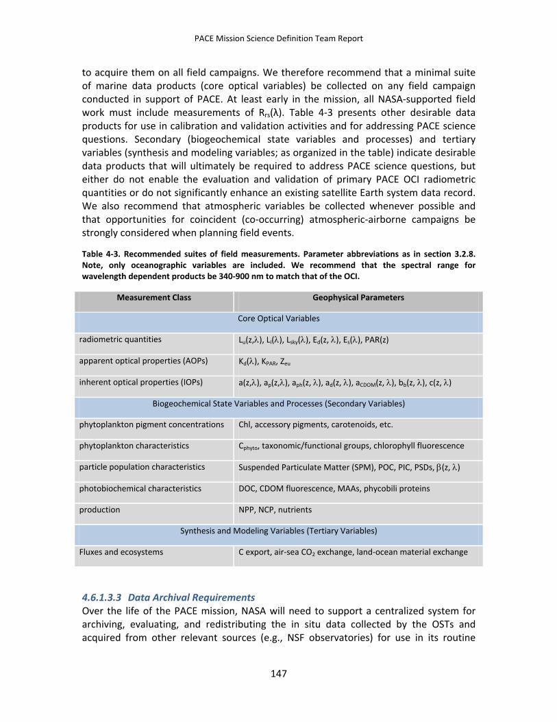
PACE Mission Science Definition Team Report
to acquire them on all field campaigns. We therefore recommend that a minimal suite of marine data products (core optical variables) be collected on any field campaign conducted in support of PACE. At least early in the mission, all NASA-supported field work must include measurements of Rrs(λ). Table 4-3 presents other desirable data products for use in calibration and validation activities and for addressing PACE science questions. Secondary (biogeochemical state variables and processes) and tertiary variables (synthesis and modeling variables; as organized in the table) indicate desirable data products that will ultimately be required to address PACE science questions, but either do not enable the evaluation and validation of primary PACE OCI radiometric quantities or do not significantly enhance an existing satellite Earth system data record. We also recommend that atmospheric variables be collected whenever possible and that opportunities for coincident (co-occurring) atmospheric-airborne campaigns be strongly considered when planning field events.
Table 4-3. Recommended suites of field measurements. Parameter abbreviations as in section 3.2.8. Note, only oceanographic variables are included. We recommend that the spectral range for wavelength dependent products be 340-900 nm to match that of the OCI.
Measurement Class Geophysical Parameters
Core Optical Variables
radiometric quantities Lu(z,λ), Li(λ), Lsky(λ), Ed(z, λ), Es(λ), PAR(z)
apparent optical properties (AOPs) Kd(λ), KPAR, Zeu
inherent optical properties (IOPs) a(z,λ), ap(z,λ), aph(z, λ), ad(z, λ), aCDOM(z, λ), bb(z, λ), c(z, λ)
Biogeochemical State Variables and Processes (Secondary Variables)
phytoplankton pigment concentrations Chl, accessory pigments, carotenoids, etc.
phytoplankton characteristics Cphyto, taxonomic/functional groups, chlorophyll fluorescence
particle population characteristics Suspended Particulate Matter (SPM), POC, PIC, PSDs, β(z, λ)
photobiochemical characteristics DOC, CDOM fluorescence, MAAs, phycobili proteins
production NPP, NCP, nutrients
Synthesis and Modeling Variables (Tertiary Variables)
Fluxes and ecosystems C export, air-sea CO2 exchange, land-ocean material exchange
4.6.1.3.3 Data Archival Requirements Over the life of the PACE mission, NASA will need to support a centralized system for archiving, evaluating, and redistributing the in situ data collected by the OSTs and acquired from other relevant sources (e.g., NSF observatories) for use in its routine
147
PACE Mission Science Definition Team Report
validation and algorithm development activities. SeaBASS, the permanent archive for field data collected under the auspices of the NASA Ocean Biology and Biogeochemistry (OBB) Program, provides these services for the SeaWiFS and MODIS time series. NASA will be responsible for the PACE mission and, therefore, needs to maintain primary responsibility for this archive. An important consideration is that the PACE mission requires that NASA house and maintain all the previous relevant data from NASA and other satellites, in situ cal/val, and other data. This data includes CZCS, SeaWiFS, and MODIS data as a minimum. As such, NASA should support the archive under its own auspices (e.g., SeaBASS) or build strong collaborative relationships with external organizations with existing capabilities (e.g., the Biological and Chemical Oceanography Data Management Office [BCO-DMO]). The co-location of the in situ data archive within the flight project, however, will yield a more fully integrated environment for satellite data product validation [Barnes et al., 2003] and we, therefore, recommend the continuation of SeaBASS for this purpose. Any system will need to provide (1) a permanent home for field data collected in support of the PACE mission, (2) clear mechanisms for version tracking and updating/replacing in situ time series, (3) reliable documentation for all data in the archive (e.g., instrument reports and descriptions of calibration practices), (4) community-endorsed mechanisms for verifying data quality and applying quality assurance metrics, and (5) efficient online utilities for rapidly and publicly re-distributing data to the research community. While the archive will be publicly accessible, we recommend that NASA adopt a policy that provides original data contributors with co-authorship rights when their data appear in community publications and presentations and/or assigns a unique and permanent identifier to each data contribution (e.g., a Digital Object Identifier) such that data incorporated into an analysis may be appropriately cited.
4.6.1.3.4 Metadata and Ancillary Data Requirements A minimal suite of metadata and raw data needs to accompany each submission to this archive. Regarding metadata: each in situ measurement must be accompanied by information on (1) sampling dates, times, locations (latitude and longitude), and depths; (2) ancillary data for each sampling event, including water depth, cloud cover, sea state, and relevant meteorological data; (3) administrative details for the experiment(s), such as the names of the principle investigator and collaborators, their contact information, and the names of the field campaign and sampling stations; and (4) references to accompanying cruise and instrument reports. We strongly recommend that all archived data be accompanied by detailed descriptions of the instruments and instrument packages used in the field and laboratory (including their calibration methods and history) and the protocols followed for data collection, processing, and analysis (including any measurement corrections applied). Furthermore, both fundamental and derived data should be archived to facilitate development of novel processing methods. For example, both absorption and absorbance (optical density) should be reported for spectrophotometric analysis of the absorption properties of particles retained on filters.
148
PACE Mission Science Definition Team Report
In this scenario, absorption (the derived product) provides the remote-sensing relevant product for use upon archival, while retaining absorbance (the fundamental measurement of the spectrophotometer) and related details, such as the volume of water filtered, permits reprocessing of absorption should novel methods for estimating filter pad amplification factors be developed. Measurement uncertainties must accompany all data products submitted to the PACE field data archive.
4.6.1.3.5 Quality Assurance Requirements Evaluating PACE-derived data products will require an abundance of consistent and high quality in situ biogeochemical data. This has previously been achieved via strict adherence to community-vetted measurement, data processing, and quality assurance protocols [e.g., Hooker et al., 2009]. We strongly recommend that the NASA ocean color flight project and OSTs (and interested members of the research community) collaborate on the development and refinement of standard protocols for collecting and evaluating marine bio-optical and biogeochemical data (see also the discussion in section 4.6.1.3.1). Activities should begin as soon as possible (no later than the formation of the first PACE OST) and continue through the life of the PACE mission. Relevant activities will include the development of data collection and processing protocols for field and laboratory instruments, standard (e.g., NIST-traceable) and community-endorsed reference materials, and standardized quality assurance metrics and uncertainty calculations. We expect the latter to facilitate the reevaluation and verification of existing in situ data sets as well—an activity that should also begin pre-launch. Current protocol documents, relevant analyses, and standardized data analysis software must be posted publicly online and routinely updated for community perusal. Furthermore, we strongly recommend that NASA routinely support community training events over the life of the PACE mission to enable hands-on dissemination of best practices in data collection, processing, and analysis.
4.6.1.3.6 Summary Without a robust calibration and validation field program and supporting OST measurement teams, the quality of radiometric data and derived biogeochemical data products from the PACE OCI will be insufficient to address the seven overarching science questions. Such activities do not currently exist at a sufficient level to support PACE. We recommend that OSTs, field programs, and other elements of a CVP established to support PACE ocean science applications include the following features:
1) Routinely formed (from present to the end of the PACE mission), revolving NASA-sponsored Ocean Science “field work” Teams to collect in situ oceanographic and atmospheric measurements
149
PACE Mission Science Definition Team Report
2) Routinely formed (from present to the end of the PACE mission), revolving NASA-sponsored Ocean Science “measurement” Teams to address satellite instrument, in situ instrument, algorithm, measurement, and data processing related issues
3) Multi-annual NASA-sponsored field campaigns (large, intensive open ocean and coastal campaigns, plus small, extensive, repeatable time-series campaigns) to collected Rrs(λ), marine biogeochemical quantities, and atmospheric measurements
4) A permanent, public data archive with NASA oversight (e.g., SeaBASS)
5) Extensive data reporting practices that require inclusion of comprehensive metadata, intermediate and ancillary data, and measurement uncertainties
To meet these minimum requirements, we strongly recommend that NASA immediately start forming PACE Ocean Science Teams; releasing research announcements for small-scale, extensive, repeatable in situ field work; and organizing large-scale, intensive field campaigns to support PACE.
4.6.2 Aerosols
4.6.2.1 Introduction The primary strategies developed to validate satellite retrievals of aerosol properties are surface-based monitoring networks, which amount to statistical comparisons with retrievals obtained from numerous near-coincident spacecraft overpasses, and more detailed, case-by-case analysis of episodic airborne measurements made as part of field campaign activities. The primary tactics employed to obtain these independent measurements include in situ measurements of aerosol microphysics, optics and chemistry, and suborbital remote sensing techniques. Each approach has limitations, such that no one suite of measurements can fully address aerosol or cloud product validation needs.
For example, surface-based sun photometer measurements have good temporal coverage (~daily), but are spatially limited, and lack the vertical resolution required to distinguish aerosol layers aloft having different compositions, as needed to constrain direct aerosol radiative forcing (DARF). Surface-based lidar measurements can distinguish layers, but only at a single point, and lack detailed information about aerosol microphysical properties and chemistry. Airborne measurements provide detailed, high-resolution (1-Hz) information on the vertical structure of aerosols, but can provide only occasional snapshots of atmospheric conditions in both space and time.
The following section outlines “Calibration/Validation Data Requirements” including a discussion of the accuracy of spectrally resolved optical data needed to validate sensor
150
PACE Mission Science Definition Team Report
retrievals for PACE and a discussion of spatial and temporal considerations. “Calibration/Validation Program Requirements” describes tools currently available for performing aerosol-focused and cloud-focused calibration/validation, as well as recommendations for further development. Discussion and recommendations presented here draw extensively from the preliminary version of the ACE satellite white paper, which serves as an invaluable compendium to this document.
4.6.2.2 Calibration/Validation Data Requirements
4.6.2.2.1 Spectral Optical Requirements Threshold: MODIS Continuity
Goal: Multi-directional, Multi-polarization and Multispectral “3M” measurements
Breakthrough: UV-VIS-SWIR measurements of absorbing aerosol
Nadir viewing spectroradiometers, such as MODIS, retrieve information about the spectral wavelength dependence of the column-averaged scattering. Independently, MODIS cannot provide information on aerosol absorption, particle morphology, refractive index, or phase function. Calibration of MODIS has been extensive, detailed, and is well documented in peer-reviewed literature. Validation of the MODIS aerosol optical depth (AOD) product has been performed by comparison with surface-based AERONET measurements over land [Levy et al., 2010] and water [Remer et al., 2008; Smirnov et al., 2010]. However, retrieval of particle microphysical properties with MODIS is hampered by relatively low information content; over water, the ratio of fine to coarse aerosol is retrieved, whereas over land, the particle optical model is effectively assumed, based on climatology [Levy et al., 2010].
Multi-angle viewing instruments provide additional information content, including some sensitivity to the vertical distribution of AOD and the aerosol phase function. Validation of the Multiangle Imaging SpectroRadiometer (MISR) has also been extensive, and led to a better constrained family of aerosol types in the retrieval algorithms used to produce geophysical data [Kahn et al., 2010]. However, the current MISR spectral bands do not contain the UV or SWIR bands needed to satisfy PACE mission requirements.
The two POLDER sensors and PARASOL were developed by CNES, and represent the first and only Multi-directional, Multi-polarization and Multispectral (i.e. “3M”) instruments to have collected data from orbit [Herman et al., 2005]. The 3M observations provide higher information content than nadir-viewing instruments, including the ability to retrieve aerosol absorption and particle morphology (e.g., spherical versus non-spherical). To date, calibration of these instruments has relied on extensive ground-based characterization of the instrument, and vicarious calibrations while on-orbit [Hagolle et al., 1999; Fougnie et al., 2007]. Although robust and reliable, and an excellent tool for deriving accurate, well validated geophysical data, the higher
151
PACE Mission Science Definition Team Report
information content could benefit from more extensive radiometric and geometric calibrations.
With these constraints in mind, adequate validation of PACE aerosol retrievals requires optical measurements that span wavelengths from the near-UV (~0.38 µm) to SWIR (~2.3 µm). To provide continuity with existing efforts requires:
1. Measurements of UV-VIS-SWIR aerosol optical depth with absolute uncertainties of +/-0.02 or relative uncertainties of 0.05*AOD
2. Measurements of UV-VIS-SWIR absorption optical depth with absolute uncertainties of less than +/- 0.02 for total AOD of > 0.1
3. Measurements capable of constraining the real part of the refractive index at UV-VIS-SWIR wavelength to better than +/- 0.02
Furthermore, breakthrough capabilities specifically required for PACE mission objectives that include a 3M-type instrument are:
4. Measurements capable of constraining single scattering albedo at UV through SWIR wavelengths to better than +/- 0.02 (i.e., uncertainty in co-albedo of < 20% at SSA of 0.90; and <50% at SSA of 0.96)
5. Measurements of refractive index, in addition to improved measurements of aerosol size distributions and particle morphology
6. Accurate polarization measurements to validate microphysical particle models
These measurements are not only germane to the validation of extensive and intensive aerosol properties, but are intrinsically linked to the validation of ocean ecosystem retrievals. The near-UV part of the spectrum is especially important, and especially challenging for PACE. Currently, the atmospheric correction for retrieving ocean color parameters, is performed by constraining aerosol optical depth (AOD) and aerosol type from several wavelengths in the red-to-near-IR part of the spectrum, and then extrapolating to the near-UV [e.g., Wang, 2007]. Uncertainties in the assumed aerosol optical models can produce large biases in these extrapolations [e.g., Ransibrahmanakul and Stumpf, 2006]. Regional differences in aerosol type, air mass spatial and temporal heterogeneity can bias ocean surface products.
4.6.2.2.2 Spatial Requirements Threshold: AERONET Continuity
Goal: Global network of UV-VIS-SWIR multipolarization observations
Breakthrough: Data coverage for global ocean
152
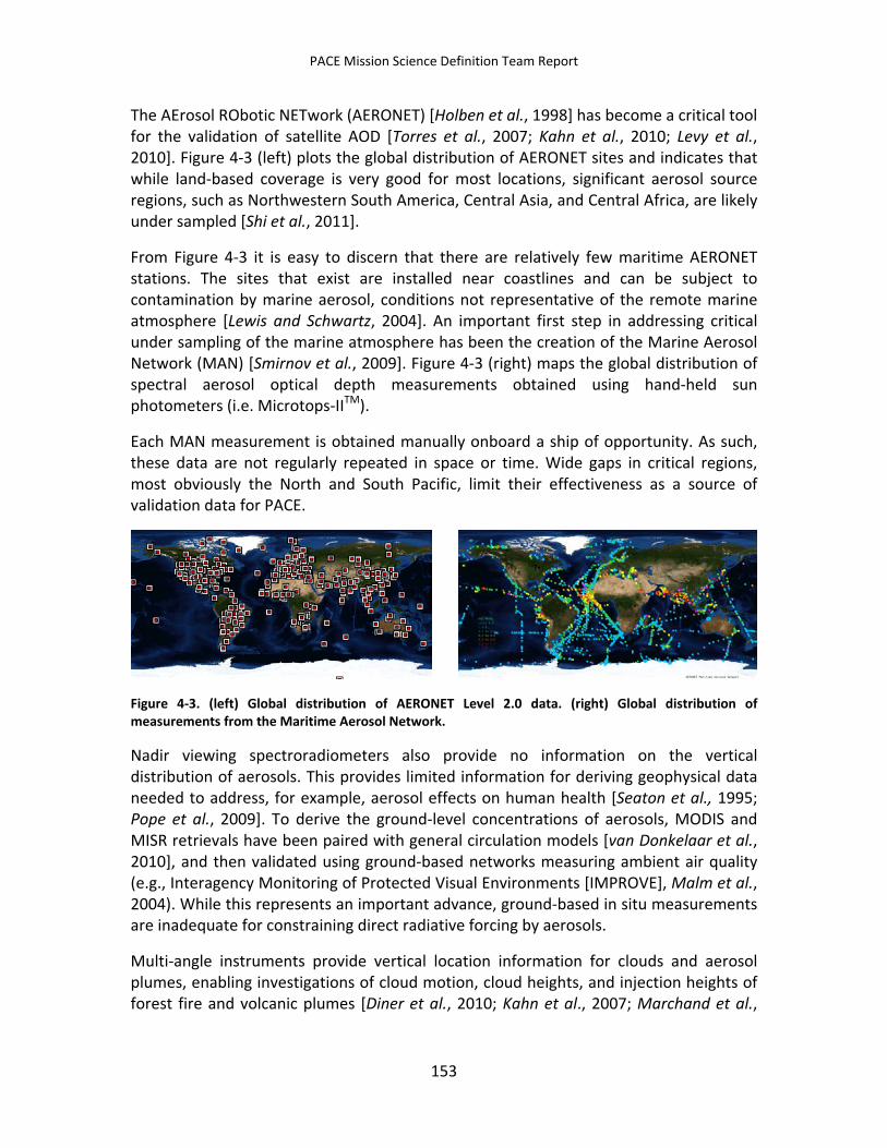
PACE Mission Science Definition Team Report
The AErosol RObotic NETwork (AERONET) [Holben et al., 1998] has become a critical tool for the validation of satellite AOD [Torres et al., 2007; Kahn et al., 2010; Levy et al., 2010]. Figure 4-3 (left) plots the global distribution of AERONET sites and indicates that while land-based coverage is very good for most locations, significant aerosol source regions, such as Northwestern South America, Central Asia, and Central Africa, are likely under sampled [Shi et al., 2011].
From Figure 4-3 it is easy to discern that there are relatively few maritime AERONET stations. The sites that exist are installed near coastlines and can be subject to contamination by marine aerosol, conditions not representative of the remote marine atmosphere [Lewis and Schwartz, 2004]. An important first step in addressing critical under sampling of the marine atmosphere has been the creation of the Marine Aerosol Network (MAN) [Smirnov et al., 2009]. Figure 4-3 (right) maps the global distribution of spectral aerosol optical depth measurements obtained using hand-held sun photometers (i.e. Microtops-IITM).
Each MAN measurement is obtained manually onboard a ship of opportunity. As such, these data are not regularly repeated in space or time. Wide gaps in critical regions, most obviously the North and South Pacific, limit their effectiveness as a source of validation data for PACE.
Figure 4-3. (left) Global distribution of AERONET Level 2.0 data. (right) Global distribution of measurements from the Maritime Aerosol Network.
Nadir viewing spectroradiometers also provide no information on the vertical distribution of aerosols. This provides limited information for deriving geophysical data needed to address, for example, aerosol effects on human health [Seaton et al., 1995; Pope et al., 2009]. To derive the ground-level concentrations of aerosols, MODIS and MISR retrievals have been paired with general circulation models [van Donkelaar et al., 2010], and then validated using ground-based networks measuring ambient air quality (e.g., Interagency Monitoring of Protected Visual Environments [IMPROVE], Malm et al., 2004). While this represents an important advance, ground-based in situ measurements are inadequate for constraining direct radiative forcing by aerosols.
Multi-angle instruments provide vertical location information for clouds and aerosol plumes, enabling investigations of cloud motion, cloud heights, and injection heights of forest fire and volcanic plumes [Diner et al., 2010; Kahn et al., 2007; Marchand et al.,
153
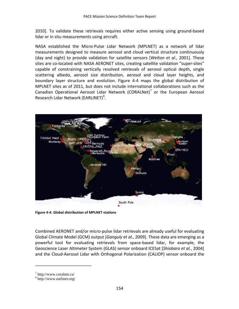
PACE Mission Science Definition Team Report
2010]. To validate these retrievals requires either active sensing using ground-based lidar or in situ measurements using aircraft.
NASA established the Micro-Pulse Lidar Network (MPLNET) as a network of lidar measurements designed to measure aerosol and cloud vertical structure continuously (day and night) to provide validation for satellite sensors [Welton et al., 2001]. These sites are co-located with NASA AERONET sites, creating satellite validation “super-sites” capable of constraining vertically resolved retrievals of aerosol optical depth, single scattering albedo, aerosol size distribution, aerosol and cloud layer heights, and boundary layer structure and evolution. Figure 4-4 maps the global distribution of MPLNET sites as of 2011, but does not include international collaborations such as the Canadian Operational Aerosol Lidar Network (CORALNet)7 or the European Aerosol Research Lidar Network (EARLINET)8.
Figure 4-4. Global distribution of MPLNET stations
Combined AERONET and/or micro-pulse lidar retrievals are already useful for evaluating Global Climate Model (GCM) output [Ganguly et al., 2009]. These data are emerging as a powerful tool for evaluating retrievals from space-based lidar, for example, the Geoscience Laser Altimeter System (GLAS) sensor onboard ICESat [Shiobara et al., 2004] and the Cloud-Aerosol Lidar with Orthogonal Polarization (CALIOP) sensor onboard the
7 http://www.coralnet.ca/ 8 http://www.earlinet.org/
154
PACE Mission Science Definition Team Report
Cloud-Aerosol Lidar and Infrared Pathfinder Satellite Observation (CALIPSO) [Berkhoff et al., 2007; Campbell et al., 2011]. Since active satellite sensors are the only means of obtaining vertically resolved aerosol and cloud information globally, assimilation of validated space-based lidar data into aerosol models and GCMs is seen as a key tool for improving these simulations [Sekiyama et al., 2010].
Equipping PACE with a 3MI-type sensor will require vertically resolved detailed measurements of aerosols and their optical properties, including polarization, in order to validate remote-sensing retrievals. MPLNET and other ground-based lidars can provide a significant part of this validation information but only at fixed locations. A limited number of new installations combined with international collaboration should ensure globally distributed coverage.
Aircraft field campaigns are regionally based, often complemented with networks of surface observations (both land- and ship-based), and often conducted in collaboration with other U.S. Federal agencies to maximize scientific return (e.g., NSF, Department of Energy [DOE], Environmental Protection Agency [EPA] and NOAA). Although these airborne field campaigns provide only a snapshot in both space and time, they have become invaluable for validating the current fleet of sensors designed to measure atmospheric trace gases, aerosols and clouds. The precision of airborne instruments and an aircraft’s ability to sample both the horizontal and vertical variability of air masses will be important tools for validating aerosol and cloud retrievals from the PACE sensor suite.
4.6.2.2.3 Temporal Requirements Threshold: AERONET continuity
Goal: Long-term global monitoring
Breakthrough: not applicable (N/A)
Over the course of their orbital lifetimes, the radiometric accuracy of sensors onboard satellites can drift. To correct for this tendency requires ongoing calibration efforts. The MODIS and MISR sensors on board NASA’s Terra mission have been obtaining high-quality environmental data for more than 12 years. These long operational lifetimes enable important observations of not only seasonal and annual variability, but are also on the cusp of being able to provide information on long-term trends [Diner et al., 2010; Zhang and Reid, 2010].
NASA needs to undertake a sustained, adequately funded suborbital calibration program over the lifetime of the PACE mission to maximize science return. As discussed, the program needs to adequately address spatial sampling requirements, including vertical profiles (e.g. MPLNET, aircraft). However, extended temporal sampling is also critically important. For example, Figure 4-3 (left) plotted all of the AERONET stations
155
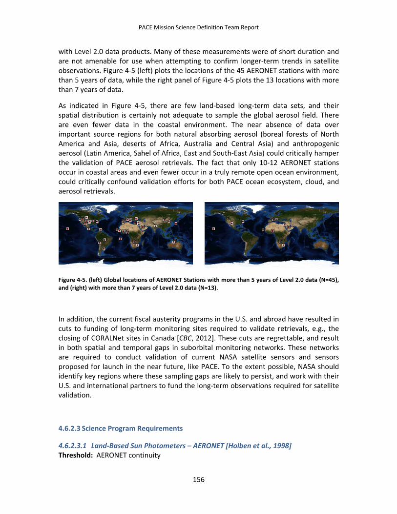
PACE Mission Science Definition Team Report
with Level 2.0 data products. Many of these measurements were of short duration and are not amenable for use when attempting to confirm longer-term trends in satellite observations. Figure 4-5 (left) plots the locations of the 45 AERONET stations with more than 5 years of data, while the right panel of Figure 4-5 plots the 13 locations with more than 7 years of data.
As indicated in Figure 4-5, there are few land-based long-term data sets, and their spatial distribution is certainly not adequate to sample the global aerosol field. There are even fewer data in the coastal environment. The near absence of data over important source regions for both natural absorbing aerosol (boreal forests of North America and Asia, deserts of Africa, Australia and Central Asia) and anthropogenic aerosol (Latin America, Sahel of Africa, East and South-East Asia) could critically hamper the validation of PACE aerosol retrievals. The fact that only 10-12 AERONET stations occur in coastal areas and even fewer occur in a truly remote open ocean environment, could critically confound validation efforts for both PACE ocean ecosystem, cloud, and aerosol retrievals.
Figure 4-5. (left) Global locations of AERONET Stations with more than 5 years of Level 2.0 data (N=45), and (right) with more than 7 years of Level 2.0 data (N=13).
In addition, the current fiscal austerity programs in the U.S. and abroad have resulted in cuts to funding of long-term monitoring sites required to validate retrievals, e.g., the closing of CORALNet sites in Canada [CBC, 2012]. These cuts are regrettable, and result in both spatial and temporal gaps in suborbital monitoring networks. These networks are required to conduct validation of current NASA satellite sensors and sensors proposed for launch in the near future, like PACE. To the extent possible, NASA should identify key regions where these sampling gaps are likely to persist, and work with their U.S. and international partners to fund the long-term observations required for satellite validation.
4.6.2.3 Science Program Requirements
4.6.2.3.1 Land-Based Sun Photometers – AERONET [Holben et al., 1998] Threshold: AERONET continuity
156
PACE Mission Science Definition Team Report
Goal: Effective and efficient spatial and temporal sampling
Breakthrough: Measurements at UV-VIS-SWIR including polarization
Figure 4-3 is a global map of stations included in the AErosol RObotic NETwork (AERONET) [Holben et al., 1998]. Each AERONET site employs a CIMELTM sun/sky-scanning radiometer, which measures direct solar radiation and the angular distribution of diffuse transmitted radiation at discrete wavelengths. From direct solar measurements, AERONET provides direct measurements of aerosol optical depth with accuracy of 0.015*cos(solar zenith angle [SZA]) at wavelengths of 380, 440, 500, 670, 870, 936, and 1020 nm, and with lower accuracy of 0.02*cos(SZA) at wavelengths of 340 and 1640 nm. Not every AERONET station has UV (340 nm) or SWIR (1640 nm) channels, though all AERONET radiometers conduct sky scanning observations of radiance in solar almucantar and principal plane at four standard wavelengths (λ = 440 670, 870 and 1020 nm). These observations are used to derive detailed aerosol microphysical and optical properties including size distribution, spectral single scattering albedo, and complex index of refraction [Dubovik and King, 2000; Dubovik et al., 2002], as well as, particle shape information [Dubovik et al., 2006].
Newer versions of the CIMELTM radiometer conduct sky-scanning observations over the UV-VIS-SWIR spectral channels. However, the accuracy of UV and SWIR sky observations is presently limited, and these data are not yet publicly available. In addition, ~5 AERONET stations are equipped with the newest models of CIMELTM radiometers conducting sky-scanning polarimetric observations over the PACE spectral channels (with exception of SWIR). These observations enable improved retrievals of aerosol properties, in particular the size distribution of aerosol fine mode, the real part of the refractive index, and particle shape [Li et al., 2009]. However, the calibration procedures for polarimetric measurements is not yet fully established or standardized within the AERONET network, and new aerosol products from the polarimetric observations are not currently publicly available.
It should be noted that the transmitted radiation observed from ground stations generally has high information content, and the existing AERONET infrastructure can serve as a basis for validation of space-based observations from a PACE polarimeter. However, current limitations in the spectral range of AERONET, and the practical absence of polarimetric observations, remain significant deficiencies and will limit their use for validation of PACE polarimeter retrievals.
As a result of these considerations, there are a number of recommendations that need to be considered as part of an effective validation program for PACE.
1) Funds for technological development and refinement of the CIMELTM instrument and/or comparable ground-sun photometers need to be made available to improve upon the existing capabilities
157
PACE Mission Science Definition Team Report
2) The distribution of AERONET sites that include UV and polarization measurements needs to be mapped to prioritize funding for the continuity of existing measurements sites, and to establish new sites for PACE validation activities
3) AERONET sites near aerosol source regions, particularly sources of absorbing aerosol, need to be upgraded to include UV, polarization, and sky scanning capabilities
4.6.2.3.2 Ocean-Based Sun Photometers – Marine Aerosol Network Threshold: Maritime Aerosol Network (MAN) continuity
Goal: Effective and efficient spatial and temporal sampling
Breakthrough: Semi-autonomous measurements at UV-VIS-SWIR including polarization
The Maritime Aerosol Network (MAN) [Smirnov et al., 2009] is a dataset of spectral aerosol optical depths measured by the hand-held Microtops-IITM sun photometer on ships at sea. Figure 4-3 shows the location of all the MAN measurements as of February, 2012.
The Microtops-II instruments have five spectral bands in one of two configurations (λ = 340, 440, 500 or 675, 870 and 936 nm). Instruments are calibrated with respect to AERONET, and therefore have slightly larger uncertainties (~+/- 0.02 compared to +/- 0.01 for AERONET) [Porter et al., 2001; Ichoku et al., 2002; Knobelspiesse et al., 2003]. Because the Microtops-II instruments only observe the direct solar beam (and not diffuse sky radiance) their data cannot be used to derive AERONET-type aerosol products such as refractive index, size and shape [Dubovik and King, 2000; Dubovik et al., 2002; Dubovik et al., 2006]. AERONET sites are limited to land or stable platforms at sea, so MAN is providing valuable validation at maritime locations far from shore. However, the Microtops-II requires a human operator, so the quantity of measurements depends on the availability of such personnel and the number of deployments during cruises at sea. For this reason, the MAN contains far fewer measurements than AERONET.
The MAN grew out of the sun photometer component of the Sensor Intercomparison and Merger for Biological and Interdisciplinary Oceanic Studies (SIMBIOS) Project. This program existed between 1997 and 2002, and was designed to aid the validation and calibration of ocean color and atmospheric products from the Sea-viewing Wide Field-of-view Sensor (SeaWiFS) and other sensors [Fargion et al., 2001; Knobelspiesse et al., 2004].
To validate PACE retrievals over the global ocean, NASA needs to improve the quality and quantity of ship-based aerosol, cloud, and ocean-color measurements. Future data
158
PACE Mission Science Definition Team Report
collection strategies should incorporate lessons learned during the SIMBIOS Project, where autonomous sun photometers such as the Fast-Rotating Shadow-band Radiometer (FRSR) [Reynolds et al., 2001; Miller et al., 2003] were developed and deployed at sea [Miller et al., 2004]. Future instruments proposed for ship-based deployment should be designed with PACE validation requirements in mind, as water-leaving radiances are inherently affected by water column constituents such as Chlorophyll-a and chromophoric dissolved organic matter, i.e. CDOM [Chowdhary et al., 2012]. Recently developed instruments that could potentially meet this observational requirement include the SeaWiFS Photometer Revision for Incident Surface Measurements (SeaPRISM), the Optical Sensors for Planetary Radiant Energy (OSPREy) and the Spectrometer for Sky-Scanning, Sun-Tracking Atmospheric Research (4STAR).
SeaPRISM [Zibordi et al., 2004] is a modified version of the AERONET CIMELTM sun photometers. The instrument includes radiometers that observe both atmospheric and water optical properties, and their observations are stored in the AERONET database (Zibordi et al., 2010). However, like AERONET sun photometers, SeaPRISM instruments must be mounted on fixed locations such as platforms at sea.
A next-generation instrument is the OSPREy [Morrow et al., 2010], which contains several instrument types in one package. The OSPREy instrument suite includes shadowband radiometers such as the FRSR, above-water radiometers, and a spectral range encompassing both the UV and SWIR. In addition, OSPREy instruments have the capability of automated sun tracking, and can therefore be deployed on moving platforms such as ships. Another option may be ship-based adaptation of second-generation sun-tracking photometers developed for use onboard aircraft, e.g., 4STAR [Dunagan et al., 2011], an upgraded version of the Ames Airborne Tracking Sunphotometer-14 (AATS-14) instrument [Russell et al., 2007; Redemann et al., 2009].
Once operational, these instruments require broad and sustained deployment aboard the global fleet of research vessels to address the critical issue of under sampling of the marine environment. Data collected as part of this at-sea network then needs to be checked for Quality Assurance/Quality Control (QA/QC), archived, and made available to the broader scientific community. Emerging examples of at-sea networks include the Shipboard Automated Meteorological and Oceanographic System (SAMOS) and the Joint Archive for Shipboard Acoustic Doppler Current Profiler (ADCP) measurements (JASADCP). The SAMOS9 project is operated by Florida State University, and is funded through a collaboration with NOAA’s Climate Observation Division. The JASADCP10 program is operated by the University of Hawaii in collaboration with NOAA’s National Coastal Data Development Center (NCDDC). Ship based ADCPs are filling key data gaps for ocean currents in the remote ocean [Chen and Firing, 2006; Len et al., 2007], with instruments deployed onboard both university research vessels (Figure 4-6, upper-row)
9 http://samos.coaps.fsu.edu/html/ 10 http://ilikai.soest.hawaii.edu/sadcp/
159
PACE Mission Science Definition Team Report
and aboard NOAA research ships (Figure 4-6, bottom-row), including NOAA’s flagship the Research Vessel (R/V) Ron Brown. A coordinated and sustained effort funded by NASA and/or NOAA to collect and archive ship-based measurements of atmospheric and water optical properties would be invaluable for validating PACE retrievals of aerosol, cloud, and ocean data products.
Figure 4-6. Data tracks for shipboard acoustic Doppler current profiler (ADCP) measurements from (top-left) R/V Kilo Moana (University of Hawai`i), the R/V Knorr (Woods Hole Oceanographic Institution), R/V Ron Brown (NOAA-Charleston, SC), R/V Ka`imimoana (NOAA-Honolulu, HI).
4.6.2.3.3 Airborne Field Campaigns Required: Sustained funding to maintain critical infrastructure
Goal: Inter-calibrated instruments on separate platforms operating globally
Breakthrough: Global measurements using unmanned aerial systems
In the late 1980s NASA created the Global Tropospheric Experiment (GTE) series of global airborne measurement campaigns to study the impact that humans are having on the global troposphere. These experiments initially focused on trace gases (CO2, SOx, NOx) but began measuring aerosols in the mid-1990s. The uses of airborne field campaigns for satellite aerosol product validation has continued to evolve and will likely
160
PACE Mission Science Definition Team Report
remain an important component of future validation activities. Investigations can be regional in scale and use only a single light aircraft [Ferrare et al., 2006]. Larger efforts can be intercontinental in scale, involve prognostic meteorology and air quality simulations at regional and global scales, and include high-resolution operation of NASA satellite sensors [Huebert et al., 2003; Singh et al., 2009; Jacob et al., 2010].
Airborne platforms that can profile from tens of meters above the ocean’s surface, to the upper-troposphere/lower-stratosphere boundary (~12 km at mid-latitudes) are required to adequately constrain aerosol retrievals. In the U.S., this capability is limited to the NASA Dryden Flight Research Center’s DC-811 aircraft and the National Center for Atmospheric Research’s High-performance Instrumented Airborne Platform for Environmental Research (HIAPER)12 aircraft, though their operation below 300 meters is typically restricted. NASA’s Wallops Flight Facility P-3B13 aircraft and the National Center for Atmospheric Research’s (NCAR) C-13014 aircraft are better suited for low-altitude flight (to 50 meters), but have flight ceilings of ~8 km with a full payload. Other small aircraft in the NASA, NSF, DOE and university-operated fleets are also very useful, but are typically limited by flight ceilings, payload capacity and endurance.
New investigations propose the use of unmanned aerial systems (UAS) [McNaughton and Mace, 2011]. The flight envelope of NASA’s Ikhana15 UAS includes the full troposphere (0.3 – 12 km), payload capabilities of up to 1200 kg, and flight endurance of up to 24 hours. While NASA’s Global Hawk16 is not suited for low-altitude in situ sampling, it is capable of carrying payloads of 1000 kg to 18 km’s. Global Hawk has a range of more than 11,000 nautical-miles and an endurance of up to 30 hours, providing sustained observing capabilities well beyond any manned aircraft.
Recently there have been significant improvements in the instruments being deployed aboard these airborne platforms, for example, instruments measuring volatile submicrometer aerosol chemistry [Canagaratna et al., 2007; DeCarlo et al., 2006] and submicrometer black carbon mass [Stephens et al., 2003]. Quantitative supermicrometer measurements of aerosol chemistry are not typically obtained in real time, but such measurements could become possible with improvements to existing qualitative techniques [Froyd et al., 2009]. Integration times for filter-based measurement can be as short as 5-10 minutes at true airspeeds > 150 m s-1 [Dibb et al., 2003]. This amounts to 45-90 km of spatial integration—coarse compared to MODIS 9-km resolution Chlorophyll-a products and proposed spatial resolution of PACE.
Separate physical techniques are required to measure the entire aerosol size distribution under ambient relative humidity, as this represents a range of ~1012 in
11 http://www.nasa.gov/centers/dryden/aircraft/DC-8/index.html 12 http://www.hiaper.ucar.edu/ 13 http://airbornescience.nasa.gov/aircraft/P-3_Orion 14 http://www.eol.ucar.edu/instrumentation/aircraft/C-130/c-130 15 http://www.nasa.gov/centers/dryden/aircraft/Ikhana/index.html 16 http://www.nasa.gov/centers/dryden/aircraft/GlobalHawk/index.html
161
PACE Mission Science Definition Team Report
aerosol mass (geometric diameters, dg = 0.01 – 100 µm). Optically active aerosols effectively range over ~109 in aerosol mass (dg = 0.1 – 100 µm). Sampling these aerosols via passive inlets is presently limited to geometric diameters <2.5 µm by aerodynamic considerations [McNaughton et al., 2007], but is effectively equivalent to the U.S. Environmental Protection Agency’s PM2.5 sampling standard. Sampling using actively controlled inlets effectively meets EPA PM10 sampling standards [Huebert et al., 2004], but deployment is limited by cost, system weight and power requirements. Unbiased sampling of mineral dust and sea salt under high humidity remains an observational challenge.
In situ airborne measurements of aerosol optical properties including aerosol light scattering (σsp), absorption (σap), and extinction (σep), and their values as a function of relative humidity (f[RH]), are currently accomplished using integrating nephelometers [Anderson and Ogren, 1998], filter-based absorption measurements [Bond et al., 1999], photo-acoustic techniques [Lack et al., 2006], and cavity-ring-down techniques [Strawa et al., 2003; Baynard et al., 2007]. Nephelometer accuracy and precision is well characterized [Anderson et al., 2003], but exists only at discrete wavelengths (σsp, λ = 450, 550, 700 nm). Absorption measurements at discrete visible wavelengths (λ = 370, 470, 520, 532, 590, 660, 880, and 950 nm) is routine [Moosmuller et al., 2009], but accuracy for instruments commonly deployed aboard aircraft [e.g. McNaughton et al., 2011] is poorly constrained [Subramanian et al., 2007; Cappa et al., 2008; Lack et al., 2008].
Recent developments in photoacoustic and cavity-ring-down techniques could meet PACE validation requirements in the UV-VIS-SWIR wavelengths [Gyawali et al., 2011]. However, instruments based on these techniques require further development and broader deployment aboard aircraft to better establish their capabilities and their reliability for satellite validation activities.
Airborne remote sensing observations are also a key tool employed to validate satellite retrievals of aerosol optical depth [Russell et al., 2007; Redemann et al., 2009]. As with the new techniques for measuring in situ aerosol optical properties, there have been promising new developments [Dunagan et al., 2011] that should extend the range of wavelengths into the UV and SWIR—a key requirement for adequate validation of PACE aerosol retrievals.
Figure 4-7 illustrates the impressive degree of closure currently being obtained between in situ measurements (University of Hawaii), suborbital remote sensing measurements (NASA Ames), and AERONET [Shinozuka et al., 2011]. Continuing to develop these airborne capabilities over UV, VIS and SWIR wavelengths, and ensuring their episodic deployment in a broad number of localities, will be critical to meeting PACE validation requirements.
162
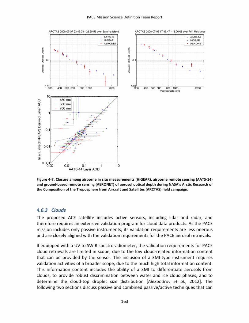
PACE Mission Science Definition Team Report
Figure 4-7. Closure among airborne in situ measurements (HiGEAR), airborne remote sensing (AATS-14) and ground-based remote sensing (AERONET) of aerosol optical depth during NASA’s Arctic Research of the Composition of the Troposphere from Aircraft and Satellites (ARCTAS) field campaign.
4.6.3 Clouds The proposed ACE satellite includes active sensors, including lidar and radar, and therefore requires an extensive validation program for cloud data products. As the PACE mission includes only passive instruments, its validation requirements are less onerous and are closely aligned with the validation requirements for the PACE aerosol retrievals.
If equipped with a UV to SWIR spectroradiometer, the validation requirements for PACE cloud retrievals are limited in scope, due to the low cloud-related information content that can be provided by the sensor. The inclusion of a 3MI-type instrument requires validation activities of a broader scope, due to the much high total information content. This information content includes the ability of a 3MI to differentiate aerosols from clouds, to provide robust discrimination between water and ice cloud phases, and to determine the cloud-top droplet size distribution [Alexandrov et al., 2012]. The following two sections discuss passive and combined passive/active techniques that can
163
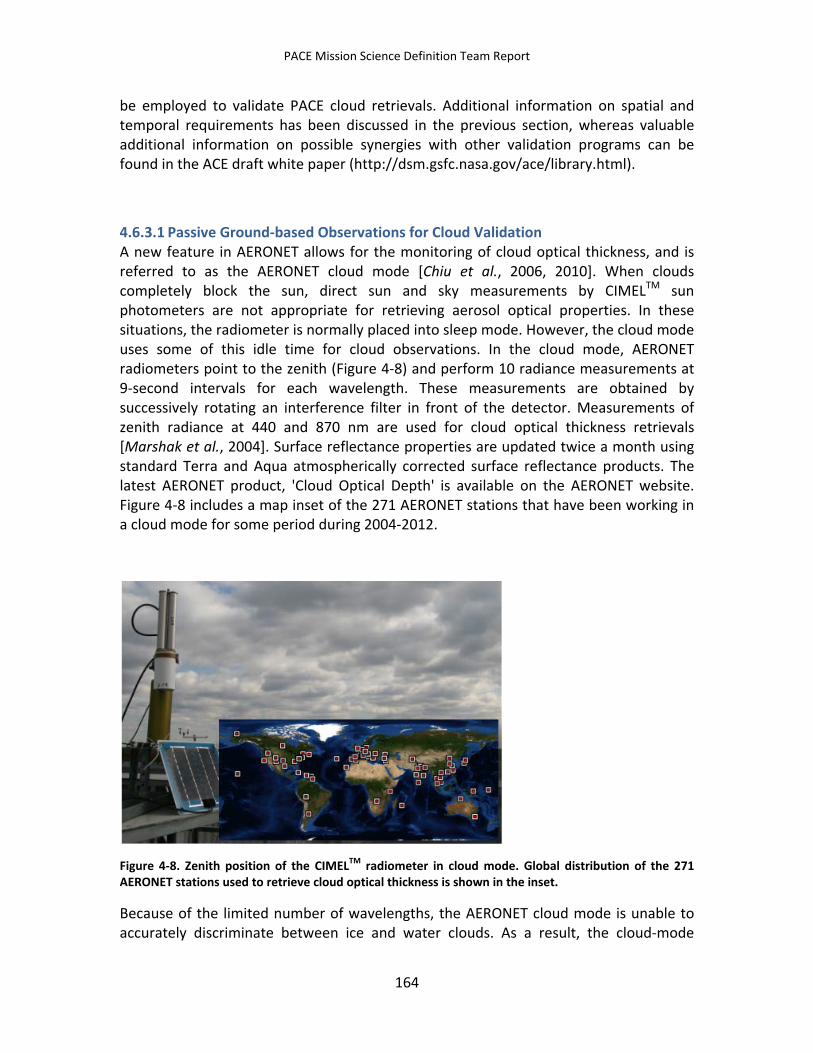
PACE Mission Science Definition Team Report
be employed to validate PACE cloud retrievals. Additional information on spatial and temporal requirements has been discussed in the previous section, whereas valuable additional information on possible synergies with other validation programs can be found in the ACE draft white paper (http://dsm.gsfc.nasa.gov/ace/library.html).
4.6.3.1 Passive Ground-based Observations for Cloud Validation A new feature in AERONET allows for the monitoring of cloud optical thickness, and is referred to as the AERONET cloud mode [Chiu et al., 2006, 2010]. When clouds completely block the sun, direct sun and sky measurements by CIMELTM sun photometers are not appropriate for retrieving aerosol optical properties. In these situations, the radiometer is normally placed into sleep mode. However, the cloud mode uses some of this idle time for cloud observations. In the cloud mode, AERONET radiometers point to the zenith (Figure 4-8) and perform 10 radiance measurements at 9-second intervals for each wavelength. These measurements are obtained by successively rotating an interference filter in front of the detector. Measurements of zenith radiance at 440 and 870 nm are used for cloud optical thickness retrievals [Marshak et al., 2004]. Surface reflectance properties are updated twice a month using standard Terra and Aqua atmospherically corrected surface reflectance products. The latest AERONET product, 'Cloud Optical Depth' is available on the AERONET website. Figure 4-8 includes a map inset of the 271 AERONET stations that have been working in a cloud mode for some period during 2004-2012.
Figure 4-8. Zenith position of the CIMELTM radiometer in cloud mode. Global distribution of the 271 AERONET stations used to retrieve cloud optical thickness is shown in the inset.
Because of the limited number of wavelengths, the AERONET cloud mode is unable to accurately discriminate between ice and water clouds. As a result, the cloud-mode
164
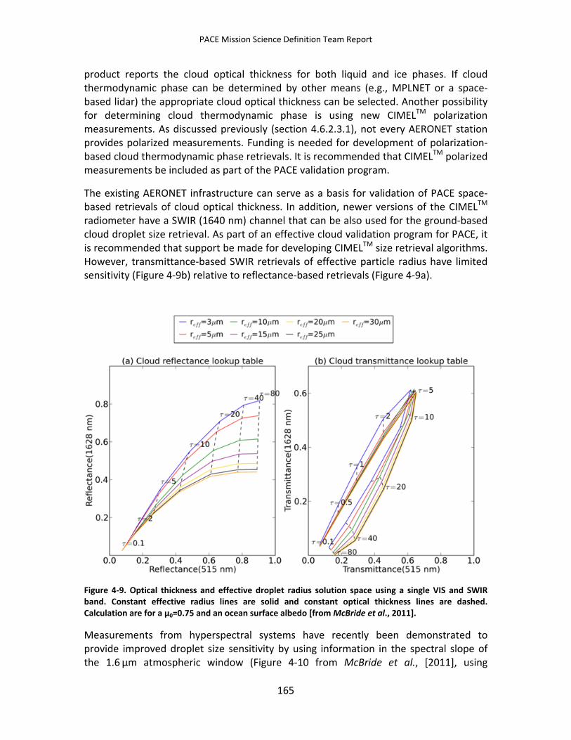
PACE Mission Science Definition Team Report
product reports the cloud optical thickness for both liquid and ice phases. If cloud thermodynamic phase can be determined by other means (e.g., MPLNET or a space-based lidar) the appropriate cloud optical thickness can be selected. Another possibility for determining cloud thermodynamic phase is using new CIMELTM polarization measurements. As discussed previously (section 4.6.2.3.1), not every AERONET station provides polarized measurements. Funding is needed for development of polarization-based cloud thermodynamic phase retrievals. It is recommended that CIMELTM polarized measurements be included as part of the PACE validation program.
The existing AERONET infrastructure can serve as a basis for validation of PACE space-based retrievals of cloud optical thickness. In addition, newer versions of the CIMELTM radiometer have a SWIR (1640 nm) channel that can be also used for the ground-based cloud droplet size retrieval. As part of an effective cloud validation program for PACE, it is recommended that support be made for developing CIMELTM size retrieval algorithms. However, transmittance-based SWIR retrievals of effective particle radius have limited sensitivity (Figure 4-9b) relative to reflectance-based retrievals (Figure 4-9a).
Figure 4-9. Optical thickness and effective droplet radius solution space using a single VIS and SWIR band. Constant effective radius lines are solid and constant optical thickness lines are dashed. Calculation are for a µ0=0.75 and an ocean surface albedo [from McBride et al., 2011].
Measurements from hyperspectral systems have recently been demonstrated to provide improved droplet size sensitivity by using information in the spectral slope of the 1.6 µm atmospheric window (Figure 4-10 from McBride et al., [2011], using
165
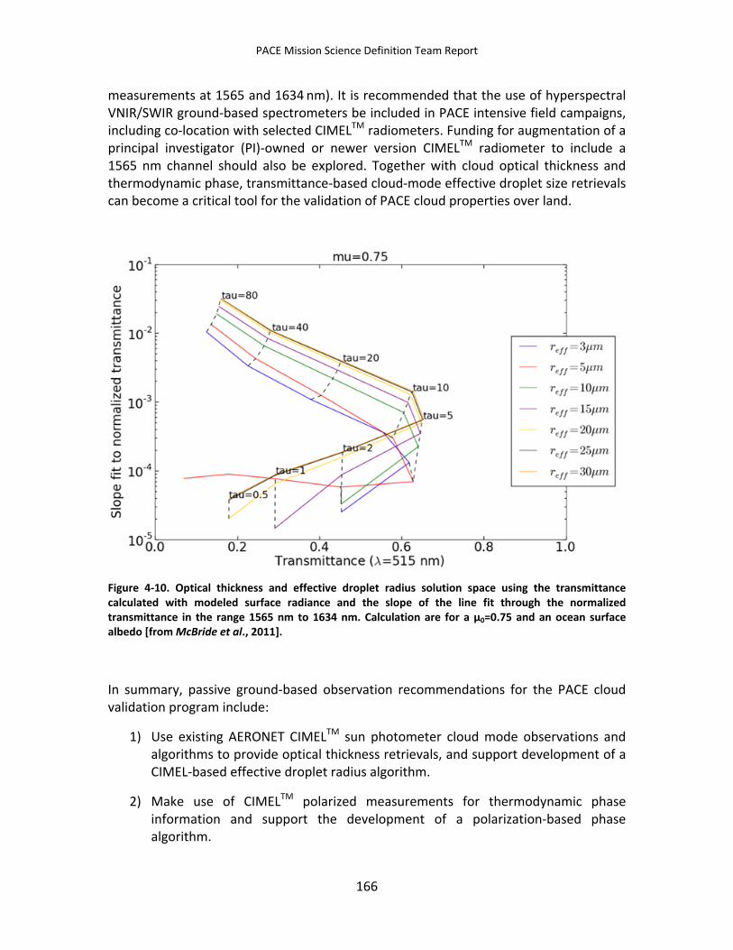
PACE Mission Science Definition Team Report
measurements at 1565 and 1634 nm). It is recommended that the use of hyperspectral VNIR/SWIR ground-based spectrometers be included in PACE intensive field campaigns, including co-location with selected CIMELTM radiometers. Funding for augmentation of a principal investigator (PI)-owned or newer version CIMELTM radiometer to include a 1565 nm channel should also be explored. Together with cloud optical thickness and thermodynamic phase, transmittance-based cloud-mode effective droplet size retrievals can become a critical tool for the validation of PACE cloud properties over land.
Figure 4-10. Optical thickness and effective droplet radius solution space using the transmittance calculated with modeled surface radiance and the slope of the line fit through the normalized transmittance in the range 1565 nm to 1634 nm. Calculation are for a µ0=0.75 and an ocean surface albedo [from McBride et al., 2011].
In summary, passive ground-based observation recommendations for the PACE cloud validation program include:
1) Use existing AERONET CIMELTM sun photometer cloud mode observations and algorithms to provide optical thickness retrievals, and support development of a CIMEL-based effective droplet radius algorithm.
2) Make use of CIMELTM polarized measurements for thermodynamic phase information and support the development of a polarization-based phase algorithm.
166
PACE Mission Science Definition Team Report
3) Include hyperspectral VNIR/SWIR spectrometers for enhanced effective droplet radius retrievals and support the development of a hyperspectral phase algorithm. As an alternative to full hyperspectral coverage, investigate the development of a second 1.6 µm window channel in existing (CIMELTM) or new filter radiometer systems.
4.6.3.2 Active/Passive Ground-based Observations for Cloud Validation The Atmospheric Radiation Measurement (ARM) Program now provides continuous baseline microphysical retrieval (MICROBASE) of cloud microphysical properties [Dunn et al., 2011]. So far, data has been released only for the three major sites (Southern Great Plains, North Slope of Alaska, and Tropical Western Pacific); there are expected to be many more sites by launch of the PACE mission. MICROBASE uses observations from the 35-GHz millimeter wavelength cloud radar (MMCR), ceilometer, micropulse lidar, microwave radiometer, and balloon-borne radiosonde soundings. Thus, MICROBASE is a combination of passive and active sensors. The product includes cloud liquid water content (LWC ) and ice water content (IWC), and liquid and ice cloud effective particle radius. Cloud optical thickness for overcast scenes is retrieved using the Multifilter Rotating Shadowband Radiometer (MFRSR) [e.g., see Min et al., 2003, 2004]. Atmospheric Radiation Measurement (ARM) passive ground-based observations have been successfully used for validation of MODIS cloud optical thickness for many years [e.g., Mace et al., 2005].
Existing lidar networks on land, such as Micro Pulse Lidar Network (MPLNET), can be used to validate PACE cloud height retrievals. MPLNET [Welton et al., 2001] measures aerosol and cloud vertical structure. However, validation by MPLNET is limited to optically thin clouds (with optical thickness smaller than 3), since the lidar signal cannot penetrate through thicker clouds; in this case it provides only cloud-base height. To validate PACE cloud height retrievals for thicker clouds, ground-based MMCR measurements are frequently used. For example, a 35-GHz MMCR is operated continuously at the ARM Southern Great Plain site and has been used to compare with cloud top heights retrieved from MODIS and MISR [Naud et al., 2005], as well as from the hyperspectral SCIAMACHY onboard EnviSat [Kokhanovsky et al., 2009]. The ground-based ARM cloud products would therefore be an important source of validation for PACE cloud retrievals.
4.6.3.3 Airborne In Situ Observations for Cloud Validation Warm Clouds: Although ground-based observations can provide estimates of cloud droplet size, the validation of these approaches has thus far been very limited and indicates significant differences between different techniques [Min et al., 2003; Feingold et al., 2006]. Some of these differences may be related to the different vertical sensitivities of the various methods (e.g., cloud optical depth from MFRSR and liquid
167
PACE Mission Science Definition Team Report
water path versus transmission using a split window in the 1.6 µm spectral region) [Platnick, 2000]. Different methods would therefore be expected to give different results if there is a strong variation in droplet size with height in the cloud. This concern is particularly relevant to the use of ground-based observations for validation of satellite microphysical retrievals, because downward looking observations have a very different vertical profile sensitivity to that of ground-based observations [Platnick, 2000] with considerably more weight towards cloud top, where droplets are usually larger. This is the reason that airborne in situ observations of cloud microphysics would be of considerable value in assessing PACE cloud droplet size retrievals [Painemal and Zuidema, 2011]; the vertical profile of droplet size can be measured and any necessary assumptions regarding vertical profile properties [Bennartz, 2007] or droplet size distribution widths can be assessed.
The in situ measurement of cloud microphysics in warm clouds is quite mature [Baumgardner et al., 2011] and the Cloud Aerosol and Precipitation Spectrometer (CAPS) suite and the Forward Scattering Spectrometer Probe (FSSP) and variants on that design have been used extensively in intensive field campaigns and sustained measurement campaigns to determine size distributions. Measurements of liquid water content using hot wire probes of various kinds are also considered to be reliable. In situ measurements of this kind can be used to validate PACE retrievals of cloud top height, cloud optical depth, droplet size distribution estimates from polarimetric observations, droplet effective radii using different spectral bands, and estimates of liquid water path.
Cold Clouds: There are three issues with regard to in situ observations of cold clouds that make the validation of PACE retrievals for such clouds more difficult than for warm clouds. The first is the issue of shattering artifacts that affect any instrument that has an inlet, or structure that could generate shattered ice in the measurement volume. One approach to dealing with this issue is to make measurements that facilitate the identification and rejection of shattering artifacts. The 2DS instrument that provides this capability has been successfully deployed in a number of field campaigns [Lawson et al., 2006] and it appears to provide reliable estimates of ice crystal size distributions. The second issue is that the scattering properties of ice crystals, and in particular their phase functions, are primarily determined by the aspect ratios of their component parts and their surface roughness, not crystal habit. Validation of the appropriateness of ice particle scattering models is essential to allow for validation of size estimates. However, the capability to estimate aspect ratio with existing instrumentation is limited and generally suffers from shattering artifacts [Korolev and Isaac, 2005; Korolev et al., 2011]. There are currently no direct in situ methods to determine ice crystal surface roughness. The only direct measurements of phase function or its first moment, which provides constraints on surface roughness, are provided by polar nephelometers [Gayet et al., 1997] or integrating nephelometers [Gerber et al., 2000]. These instruments may also suffer from shattering artifacts, and although they have provided provocative results, cannot yet be regarded as definitive validation tools. There are also recently developed instruments that use novel approaches to measuring scattering on ice crystals, and
168
PACE Mission Science Definition Team Report
show considerable promise in constraining their scattering properties [Kaye et al., 2008; Cotton et al., 2010; Abdelmonem et al., 2011]. The last issue with in situ observations of cold clouds is that such clouds are generally high enough that the availability of airborne platforms that allow such observations to be made is very limited.
4.7 Data System Requirements The PACE mission will require a data system for the acquisition, processing, archival, and distribution of all Earth observation data and onboard calibration and spacecraft and instrument engineering telemetry produced by the PACE sensor(s). The processing system and associated software must take raw, uncalibrated observations of spectral radiance exiting the top-of-the-atmosphere (TOA) and produce derived geophysical products, temporally and spatially composited to global grids. The data distribution system must be capable and efficient to support large data volumes and to provide the research community with the data it needs in a timely fashion (e.g., <1 day).
4.7.1 Data Levels and Formats The raw data, as it is acquired from the sensor, is referred to here as Level-0. Higher-level data products include:
• Level-1A: uncalibrated but potentially reformatted TOA Earth observation data
• Level-1B: calibrated TOA radiances
• Level-2: derived geophysical products
• Level-3: spatially and/or temporally composited geophysical products (e.g., daily, weekly, monthly global products on an Earth-fixed projection)
Level-1A/B and Level-2 data will be defined in the original observation grid, with geolocation information available for each pixel. The Level-1, Level-2, and Level-3 data products generated from PACE should be produced in a portable and self-describing format that follows one of the Earth Observing System Data and Information System (EOSDIS) format standards, e.g., Network Common Data Format version 4 (netCDF4) with Climate and Forecast (CF) compliant meta-data. The adoption of such a format standard provides interoperability with many analysis and visualization tools in common use by the research public, and ensures ease of integration with existing NASA data access and distribution systems.
169
PACE Mission Science Definition Team Report
4.7.2 Processing Software Processing software will be required to convert the PACE sensor data from Level-0 to higher level derived products. While similar software currently exists to support the processing of SeaWiFS, MODIS, and other sensors, and this software could be adapted to support PACE, substantial new development will be required to exploit the advanced capabilities of the PACE sensor. Algorithms developed within the PACE Science Team for the PACE ocean color sensor, including methods for atmospheric correction and bio-optical algorithms, will have to be integrated into the Level-1B to Level-2 processing code. Sensor-specific algorithms for instrument telemetry conversion and application of calibration and characterization knowledge will need to be developed and implemented for the Level-0 to Level-1A and Level-1B processing. All software developed for the processing of PACE sensor data from Level-1A through Level-3 should be open source and publicly distributed. The open source model has been vital to heritage ocean color missions, as it provides fundamental and indisputable documentation on the algorithms employed, presents a mechanism for external review and verification, and enables international collaboration and community contribution to algorithm and application development.
4.7.3 Data Ingest The PACE mission is expected to produce very large data volumes from the hyperspectral OCI: volumes on the order of 100GB/day for the Level-0 data at the nominal 1-km spatial resolution (before compression). Level-0 data will likely be downlinked multiple times per day, so the data ingest system must be fully automated and sufficiently robust to support 24x7 hands-off data acquisition.
4.7.4 Data Processing The data processing system must also be fully automated and scaled to support processing of newly acquired PACE sensor data from Level-0 through Level-3, while also supporting periodic mission reprocessings that incorporate new algorithms or improvements in instrument calibration knowledge. To support near-real-time applications, such as a need for ocean color imagery to support in situ validation efforts, the Level-2 data products should be available within hours of observation. System throughput requirements are also driven by the expected frequency of reprocessing events. Based on experience with previous sensors, it is likely that reprocessing will be required at roughly 6-month intervals for the first two years, and on one- to two-year intervals in subsequent years. Given that knowledge of sensor temporal calibration will generally evolve over time, the reprocessing will typically start from Level-1A uncalibrated radiances. To minimize disruption to ongoing research efforts, the data system should be scaled for sufficient throughput to support complete mission reprocessing from Level-1A to Level-3 in less than one month. This means processing
170
PACE Mission Science Definition Team Report
throughput capacity must grow as the mission data record grows. The processing system should also be capable of more frequent, partial-mission reprocessings to support calibration and algorithm development and quality assessment activities that are critical to achieving geophysical time-series products of sufficient quality for climate research. As advanced processing algorithms are developed or revised instrument calibrations are proposed, global life-of-mission processing tests must be performed to assess the impact to geophysical trends. For SeaWiFS and MODIS, these mission test processings entailed generating a 4-day global product for every 32-day period of the mission lifespan, or a reprocessing of 1/8th of the mission, so that global time-series trends could be analyzed. The processing system should be capable of performing such large-scale test reprocessings in 1-2 days, as changes to the data record must be evaluated incrementally and the modify-reprocess-evaluate cycle is often iterative. Reduced processing performance will slow progress toward climate-quality product development, and delay reprocessing and redistribution of improved datasets to the research community.
4.7.5 Data Archival The data system must be capable of tracking, storing, and efficiently retrieving all data acquired and produced from the PACE mission, including Level-0 through Level-3 products and multiple test processings variants. The Level-0 data must be well protected (e.g., mirrored Redundant Array of Independent Disks-6 [RAID-6] technology, offsite redundancy) to ensure the integrity of the source data throughout the active mission phase.
4.7.6 Data Distribution The data system must provide efficient and effective methods for the distribution of source data and derived products to the research community. To support timely delivery, all data should be online and directly accessible via public internet protocols. Given the large data volumes involved, the distribution systems must provide mechanisms to target the data to the research needs of the end user. This should include visual browsers for Level-1, Level-2, and Level-3 products, as well as capabilities for bulk ordering of global or regional data over any mission time-period, options for parameter and subscene extraction, and support for user-scripted automated downloads. The data distribution should specifically include uncalibrated Level-1A data, as this allows large users to maintain local archives of PACE data that would not need to be reacquired after a reprocessing.
171
PACE Mission Science Definition Team Report
4.7.7 Analysis Software and Tools The data derived from the PACE mission will not be fully exploited without efficient and user-friendly tools to visualize and analyze the products. The development and maintenance of software packages for data processing and visualization should be viewed as an integral part of the mission. An example of such a software package is the SeaWiFS Data Analysis Systems (SeaDAS), which includes both the tools to visualize and analyze all NASA ocean color data products, as well as the source code, build environment, and run-time environment that enable research users to locally reprocess from Level-1A through Level-3. SeaDAS, or a similar software package, should be developed or adapted for PACE, as it enables community algorithm development and allows end users to generate alternative or region-specific products to fully exploit the research and application capabilities of the PACE sensors. Distribution of the Level-1A to Level-1B processing capability also allows external institutions to maintain archives of Level-1A data that can be locally reprocessed when the instrument calibration is updated, thus eliminating the need to reacquire the archive after each mission reprocessing and significantly reducing the network and data distribution load.
4.7.8 User Support The PACE mission will require a responsive and knowledgeable user support team to facilitate data access, help with software issues, and generally educate the end users on the use of the data and support tools.
4.8 Integrated Data System and Data Quality Support Team The development of geophysical products of sufficient quality for climate research from spaceborne radiometric observations requires significant efforts in sensor calibration, product validation, software development, and data systems. These elements must be closely coordinated, as the process to improve and verify product quality is inherently iterative and computationally intensive (Figure 4-11). This process requires an integrated team of scientists, calibration and data systems engineers, software developers, and scientific analysts that fully understand the measurement science and have access to the complete mission archive and significant processing resources. Trends in product time series must be systematically evaluated throughout the mission to detect and separate residual sensor calibration or algorithm errors from real geophysical variability. Improvements in sensor calibration knowledge and proposed enhancements to processing algorithms must be implemented and evaluated on global, life-of-mission scales to assess impact to the time series and agreement with field measurements. Results of these analyses then provide feedback for further improvement. We strongly recommend the development of an integrated data support team (IDST), co-located with the processing system, to consolidate these core elements and to provide the data archive, distribution, and user support for the research
172
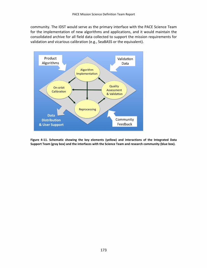
PACE Mission Science Definition Team Report
community. The IDST would serve as the primary interface with the PACE Science Team for the implementation of new algorithms and applications, and it would maintain the consolidated archive for all field data collected to support the mission requirements for validation and vicarious calibration (e.g., SeaBASS or the equivalent).
Figure 4-11. Schematic showing the key elements (yellow) and interactions of the Integrated Data Support Team (gray box) and the interfaces with the Science Team and research community (blue box).
173
PACE Mission Science Definition Team Report
5 Relationship Between PACE and Other Programs
5.1 Synergies with Future Ocean Missions In the late 1990s, NASA initiated the Sensor Intercomparison and Merger for Biological and Interdisciplinary Oceanic Studies (SIMBIOS) project and the international space agencies agreed to support the International Ocean-Colour Coordinating Group (IOCCG, www.ioccg.org). The SIMBIOS project (1997-2003) was managed out of NASA GSFC, focused on both satellite and in situ data quality, and included a competed international science team. The IOCCG activities include annual meetings of agency representatives, regular distribution of newsletters, and a series of topical reports (currently eleven published with several others in progress) authored by members of the research community. More specific IOCCG areas of interest include strategies on in situ data collection, sensor requirements, data access, geophysical algorithms, applications of ocean color data, coordination/cooperation between agencies, etc. Two of the more recent concepts that have been a focus of the IOCCG are the International Network for Sensor InTercomparison and Uncertainty assessment for Ocean Colour Radiometer (INSITU-OCR) and a virtual constellation of ocean color missions. The INSITU-OCR would be very similar to SIMBIOS, but would incorporate lessons learned from SIMBIOS and other more recent experience and would be more international in its implementation and execution. As for the constellation, there are a number of future ocean color missions that are approved or being considered. Two international low-Earth orbit (LEO) missions with global coverage that are approved and will overlap with PACE are Japan’s Second generation GLobal Imager (SGLI) on Global Change Observation Mission-3 (GCOM-3) and ESA’s Ocean Land Colour Instrument (OLCI) on the Sentinel-3 series.
While the PACE OCI will provide spectral coverage well beyond any ocean color sensor to date, SGLI and OLCI will complement PACE in several ways. SGLI is expected to launch in 2013. The sensor has ocean color bands at 380, 412, 443, 490, 530, 565, 674, 763 and 869 nm with a 250 m spatial resolution. The launch schedule for the Sentinel-3 series (three missions) is unclear at this time, but the first platform was originally scheduled for 2013. The OLCI has ocean color bands at 400, 412, 443, 490, 510, 560, 620, 665, 674, 681, 709, 753, 865, and 1020 nm with a 300 m spatial resolution. Thus, both SGLI and OLCI provide significant improvements in spectral coverage and spatial resolution over the heritage U.S. sensors (SeaWiFS, MODIS, VIIRS). Given that both will also be launched well in advance of PACE, data from these missions will allow for the evaluation of advanced geophysical product algorithms, collaboration on field programs and related infrastructure, and initiation of research on many (but not all) of the PACE scientific themes. NASA should continue to pursue bilateral agreements with the Japan Aerospace Exploration Agency (JAXA) and ESA consistent with the INSITU-OCR, especially with respect to data access. Such agreements would also facilitate the development and distribution of community software (e.g., SeaDAS) that support the processing and
174
PACE Mission Science Definition Team Report
analysis of ocean color data, as well as the merging of multiple data sets into global ocean color time series with the most complete coverage possible.
5.2 PACE Mission Applications – Ocean NASA has demonstrated the value of science-quality Earth observations in a wide range of practical applications using missions that were the precursors of PACE, including SeaWiFS and MODIS. With advanced global remote sensing capabilities that include global hyperspectral imaging, extended spectral coverage to the UV and SWIR, and improved spatial coverage, the PACE mission is expected to provide high quality observations that, over the long-term, will contribute to an extended time series of records on inland, coastal, and ocean ecosystems—all which have substantial value beyond basic science and research. PACE also offers an opportunity to fly a multi-spectral, multi-angle polarimetric imager that would add significant capabilities to extend high-quality space-based observations on the type and distribution of clouds and aerosols. These long-term ocean and atmosphere records are essential to build a baseline against which to gauge the health of the resources on our planet, to quantify patterns of variation required in models of the Earth, and to detect change similar to that detected via image analysis in the medical field.
The National Research Council (NRC) stated in its first decadal survey for Earth science that the consideration and planning for practical benefits from future satellite missions should play an equal role to that of acquiring new knowledge about Earth. In the short- and long-term, the scientific and applications-oriented objectives of NASA's PACE mission should complement one another. Science will enable improved decision making, and the practical benefits of the mission will build interest in further scientific discovery (http://appliedsciences.nasa.gov/missions.php). PACE observations will benefit a broad spectrum of public groups, including operational users in various tribal, local, state, federal, and international agencies; policy implementers; the commercial sector; scientists; educators; and the general public. The combination of high-quality, global atmospheric and oceanic observations provided by the PACE mission will provide direct benefits to society in the following major NASA application areas: Climate, Water Resources, Ecological Forecasting, Disasters, Oceans, Human Health and Air Quality.
The PACE mission will make near-daily observations across the globe, with more frequent measurements at high latitudes. These observations will provide dynamic maps of a number of critical parameters that are needed to understand the location, status, variation, and trends in important ecosystem services. The measurements will be based on rapid, frequent, repeated and long-term visible radiometry, including very subtle changes in the color of water.
Many applications in coastal, estuarine, and inland waters require high spectral and high spatial resolution (better than 1 km2) space-based observations to resolve the complex optical signals and biogeochemical processes typically characterizing these
175
PACE Mission Science Definition Team Report
environments [NRC, 2011; Table 2.2]. The medium (1 km) to high (250 to 500 m) spatial resolution observations from PACE will be particularly advantageous for research and societal applications in lakes, estuarine, and coastal environments, where environmental properties and the distribution of resources change rapidly over shorter distances than in the open ocean. The higher 250-500 m spatial resolution of PACE indeed provides a unique opportunity to extend routine assessments to a narrow zone of less than a few kilometers of the coasts of the global ocean. This capability will help to assess the value, determine cumulative impacts, and detect change and status of coastal and estuarine resources across the entire planet, consistent with the global and climate-assessment scope of the PACE mission. More specifically, PACE applications of the high spectral and spatial resolution observations include the monitoring of fisheries, water quality, and small features in the water in lakes, estuarine and coastal regions. Some examples include mapping suspended sediment plumes; understanding the direction and frequency of sediment resuspension and transport; determining the impact of river plumes on adjacent environments and patterns of connectivity; assessing conditions that affect seagrasses and coral reefs; improved detection, forecasting, and early warnings of harmful algal blooms (HABs); and improved models of abundances of fecal coliforms such as Vibrio sp. and nuisance species like sea nettles that affect human health and the value of property.
Applications of PACE satellite imagery, notably in coastal and inland environments, will require accurate atmospheric correction. Particularly in coastal areas close to polluted urban centers, PACE observations will need to be corrected for absorbing and scattering aerosols and also for other absorbing atmospheric constituents associated with anthropogenic emissions, such as NO2. An advanced multi-angle, multi-spectral polarimetric imager flown on PACE would provide the capability to advance and improve atmospheric correction for both scientific and practical applications. The possibility of a multi-angle polarimeter also offers observations of the polarized characteristics of light reflected by these aquatic environments.
5.2.1 Applications to Improve the Use of Aquatic Ecosystem Services PACE will provide high-quality observations needed to implement ecosystem-based management approaches to fisheries and the use of water resources. PACE will help advance the valuation of coastal and marine ecosystems. Placing a value on the various resources and environments humans use is required to help plan for any possible economic and social impacts that result from changes in our use of these ecosystem services. PACE will help refine measurements of primary productivity in coastal environments, of the make-up of biological communities, and of ecosystem structure needed to help improve the way we use these resources.
An important application is the mapping of ecological fronts using new and detailed measurements in the visible spectrum of light. This includes mapping and characterizing the biological features that are associated with physical circulation structures like the
176
PACE Mission Science Definition Team Report
Loop Current and eddies in the Gulf of Mexico, and with the Gulf Stream and large convergence and divergence zones that cross major sections of our oceans. These areas all serve as areas of aggregations for fish, turtle, and other organisms. The PACE data will inform decisions on where we should focus or limit fishing more actively to properly manage our fisheries. As our planet changes, we will be able to observe how the spawning habitats of different species of organisms change, and where ecological conditions make life possible for these species as they adjust their range and life cycles. PACE observations will help us to better understand essential fish habitats, the changing environment that sustains coral reefs and sea grasses, and the productivity dynamics of the phytoplankton that forms the base of the global ocean food web.
The assimilation of PACE satellite imagery into computer simulations of the ocean, atmosphere, and land components of the Earth system will lead to major advances in ecological forecasting, contributing to a better understanding of the processes that control the diversity of marine organisms and ecosystems, their distribution, and how they change over time. Understanding these features is a fundamental requirement to developing applications in pharmaceutical research, and to understanding how to best manage the productivity of natural and man-managed systems. Assimilation of PACE satellite-derived optics and biogeochemical variables into ocean models will be critical for improving model skills and forecasting capabilities.
5.2.2 Ocean and Human Health Hazards: Assessing Hazards to Human Life and Property
Sustaining the health and resilience of our marine ecosystems is a high national priority [NRC, 2011]. With the development of the National Policy for the Stewardship of the Oceans, Our Coasts, and the Great Lakes17 our country has committed itself to “protect, maintain, and restore the health and biological diversity of ocean, coastal, and Great Lakes ecosystems and resources”. PACE will generate global maps of aquatic and coastal water quality and transparency several times per week, and more often at high latitudes where significant changes are being observed in coastal and marine ecosystems. The PACE measurements are required to monitor water quality in estuarine and coastal areas, in the Great Lakes and in other inland waters close to cities and communities where people swim, fish and conduct various recreational and cultural activities. PACE synoptic observations of water transparency will help understand the conditions that lead to changes in eutrophication of waters. Knowledge of these conditions will help us to understand the causes and extent of hypoxia in coastal environments and in the deep ocean where hypoxia seems to be covering larger areas with time.
PACE-enabled space-based monitoring of ocean conditions and dynamics will be particularly beneficial to emergency managers and community decision-makers who can
17 Exec. Order No. 13547, 3 C.F.R. (2010).
177
PACE Mission Science Definition Team Report
use Earth observations to meet the challenges associated with disasters. PACE will facilitate monitoring of the effects of hurricanes on ecosystems, as well as tracking of atmospheric phenomena and disturbances (e.g., volcanic ash and fires). Including a multi-spectral, multi-angle polarimetric imager on PACE would provide additional critical information to assess impacts of atmospheric events on ecosystems and human health, and enable a path to further study the practical applications of a capability not available at present on operational sensors. Applications to emergency management and response would be greatly enhanced if there is the ability to obtain PACE data in near-real time.
The PACE measurements will add to our capabilities to detect and monitor oil spills and oil seeps, with significant improvements to the technology available during the 2010 Deepwater Horizon tragedy in the Gulf of Mexico. An application of similar importance is the detection, tracking, and forecasting of Harmful Algal Blooms (HAB), such as red tides, and the accumulation of various other algae in coastal zones. These accumulations can have significant health and economic impacts, and PACE observations can help inform the public of the causes and possible solutions to these problems. Ecological forecasting using various numerical simulations and scenarios of large-scale conditions is also important to evaluate where HABs may occur, and where there may be other possible threats to species that sustain the diversity on which we depend.
In addition, PACE will provide significant advances to shipping and navigation. It will not only allow better mapping of currents to assist the shipping industry in scheduling and in fuel economy strategies, but it will also help monitoring of sea ice extent and passages.
PACE will provide useful information that complements a long history of observations on global clouds and aerosols. The societal benefits and practical applications related to air quality and the atmospheric measurements from PACE are discussed further in section 5.3.
5.2.3 Developing a Carbon Economy PACE will contribute to the short-term assessment of carbon sources and sinks, and to the long-term measurements needed to understand changes in the carbon balance between the ocean, the land, and the atmosphere. This knowledge is needed to properly manage a carbon economy, and enables research of the carbon cycle, mapping of carbon reservoirs and fluxes in the atmosphere, and greater understanding of the biological and non-biological processes that affect the Earth System. PACE will provide an improved understanding of the biogeochemistry of elements involved in impacts and feedbacks of the climate system.
178
PACE Mission Science Definition Team Report
5.2.4 Summary In summary (see Table 5-1), the PACE mission will provide the frequent global synoptic observations from space that are required to improve our quality of life by helping assess the status of our natural and man-made resources. The PACE mission will provide unprecedented spectral (hyperspectral) and spatial (250 m to 1 km) extended records on conditions that affect the ecology and biogeochemistry of our planet. The opportunity to provide polarimetric measurements with the PACE mission offers the possibility to further extend data records on clouds and aerosol composition and dynamics. These measurements will provide a unique capability to help understand changes that affect our ecosystem services; implement science-based management strategies of coastal, marine and inland aquatic resources; and support assessments, policy analyses, and design approaches to planning adaptation and responses to impacts of climate change.
179
PACE Mission Science Definition Team Report
Table 5-1. PACE Mission: Major contributions to NASA application areas
Climate System
Carbon cycle research, mapping/assessment of carbon sources and fluxes, improved understanding of the biogeochemistry of elements involved in impacts and feedbacks of the climate system, improvement of climate model skills/forecasting capabilities, support of assessments, policy analyses, and design approaches to planning adaptation and responses to impacts of climate change.
Oceans, Coasts, Great Lakes - Ecosystems and Human Health
Fisheries and ecosystem health management; mapping of suspended sediment plumes; monitoring of water quality, including transparency, eutrophication, hypoxic conditions, sediment resuspension and transport; impacts of river plumes on adjacent environments; patterns of connectivity; monitoring of oil spills and seeps; detection of harmful algal blooms (HABs); improved models of abundances of toxic pollutants, pathogens, bacteria that affect human and ecosystem health; monitoring of sea ice extent and passages; mapping of currents (applications to shipping industry, scheduling/fuel economy strategies).
Ecological Forecasting
Forecasting and early warnings of HABs, endangered species, vertebrates diversity and distribution, biodiversity, fisheries; PACE data assimilation into ocean models for improving model skills and forecasting capabilities.
Water Resources
Water quality and management of water resources in lakes, coastal areas and open oceans.
Disasters
Effects of hurricanes on ecosystems, oil-spills and oil seeps; tracking of volcanic ash, fires and impacts on ecosystems and human health.
Air Quality and Human Health*
Air quality monitoring, forecasting, management; climate change effects on public health and air quality; aerosols, clouds, volcanic ash/aviation hazard applications (see also section 5.3).
* Many of the air quality applications would be significantly enhanced with an advanced multi-angle multi-spectral polarimetric imager.
5.3 PACE Mission Applications – Atmosphere/Aerosols The PACE Mission is focused on understanding ocean ecology and the global carbon cycle and how it affects and is affected by climate change. These data will extend observations of ocean ecology, biogeochemical cycling, and ocean productivity begun by NASA in the late 1990s. To achieve these objectives, enhanced methods of atmospheric correction are required to account for the effects of absorbing and scattering aerosol in the Earth’s atmosphere—signals that mask or alias ocean-color retrievals. These auxiliary atmospheric measurements will augment NASA’s satellite observations of
180
PACE Mission Science Definition Team Report
aerosol and clouds. Many of the applications outlined below presuppose an advanced multi-directional, multi-polarization, and multispectral imager (i.e. 3M).
The radiative effects of aerosols and clouds have been identified by the Inter-governmental Panel on Climate Change [IPCC, 2001 and 2007] as the largest source of uncertainty in our efforts to predict climate change [IPCC, 2007]. Space-based cloud and aerosol observations are also needed by regulatory agencies, resource managers, weather forecasters, and first responders. Recognizing this need, the 2007 NRC report Earth Science and Applications from Space: National Imperatives for the Next Decade (commonly referred to as the Decadal Survey) specifically states, ‘societal needs help to guide scientific priorities more effectively and that emerging scientific knowledge is actively applied to obtain societal benefits.’
Aerosol measurements with a 3MI-like instrument can augment retrievals by other NASA satellites and provide direct benefits to society. Potential applications of the PACE data include better assessments of local and regional air quality (a public health application) and better characterization of hazards for issuing disaster warnings (a public safety application).
5.3.1 Improving Ambient Air Quality Forecasts, Monitoring and Trends If an advanced multi-directional, multi-polarization, and multispectral imager is included in the PACE mission, it could provide significant contributions toward improving the monitoring of air quality and air quality forecasting. Aerosols with aerodynamic diameters less than 2.5 µm are commonly referred to as PM2.5 by air quality practitioners, and are a federally regulated pollutant due to their deleterious effects on human health [Pope et al., 2009; Seaton et al., 1995]. MODIS and MISR aerosol retrievals have already been combined with ground-based monitoring networks and space-based lidar data from CALIPSO, as well as general circulation models to evaluate public exposure to PM2.5 over the continental U.S. and globally [Liu et al., 2007; van Donkelaar et al., 2010]. Continuity of these measurements using PACE and other NASA satellites will allow NASA and U.S. policymakers to determine the effectiveness of air pollution control initiatives. For example, PACE data could be used to study decadal trends in population exposure to PM2.5, or to evaluate haze levels in areas designated as visually protected environments, i.e., National Parks in the U.S. and internationally.
The last five-year period has seen rapid operational implementation of aerosol and air-quality forecasting systems throughout the world. Largely based on infrastructure inherited from Numerical Weather Prediction (NWP), the assimilation of near-real-time (NRT) aerosol observations is recognized as an essential ingredient for accurate air-quality forecasts. Through participation in the International Cooperative for Aerosol Prediction (ICAP) (http://bobcat.aero.und.edu/jzhang/ICAP/index.html), a cooperative of aerosol system developers looking towards the next generation of aerosol models, the PACE Mission is expected to work with national and international partners to ensure
181
PACE Mission Science Definition Team Report
broad utilization of the PACE data products, for both research and operational use. Global aerosol forecast systems exist at the Naval Research Laboratory (NRL)/Monterey, European Centre for Medium-Range Weather Forecasts (ECMWF), NASA Global Modeling and Assimilation Office (GMAO), and Japan Meteorological Agency (JMA), and are currently in development at NOAA/National Centers for Environmental Prediction (NCEP) and the United Kingdom Met Office (UKMO). An overview of current aerosol forecast capabilities can be found on the ICAP webpage (http://bobcat.aero.und.edu/jzhang/ICAP/AERP-Overviews.html). Furthermore, The U.S. EPA, NOAA, National Park Service (NPS), and tribal, state, and local agencies have recently developed nationwide daily air quality forecasts and near real-time reporting of air quality through the use of Air Quality Indices (AQI17) at the AirNow website (http://airnow.gov/). Integration of future satellite data (e.g., VIIRS, PACE, Geostationary Coastal and Air Pollution Events [GEO-CAPE]) with these databases should continue to support these forecasts, enabling more and better public awareness of potentially deleterious air quality events that can adversely affect susceptible individuals. Table 5-2 represents a traceability matrix of the PACE-related aerosol measurements with applications related to air quality that would be enabled by the addition of a 3MI-like sensor.
The PACE Mission will provide broad support for the next generation of climate and numerical weather prediction models. There is general agreement across the aerosol community that aerosol data assimilation, and radiance assimilation in particular, will feature prominently in the next generation of Earth system models used for assessment of the current and past climate record. State-of-the-art data assimilation methodologies share the same optimal estimation framework that is being adopted by the PACE mission retrieval activities. Such commonality in approach offers great opportunity for synergisms between these two communities. Although the assimilation of PACE radiances is the ultimate objective in several operational centers, the NRT availability of aerosol retrievals is still necessary for the broader utilization of the PACE measurements.
182
PACE Mission Science Definition Team Report
Table 5-2. Air Quality Applications Traceability Matrix for a PACE mission that includes an advanced multi-directional, multi-polarization, and multispectral imager
Science Objectives Measurement Objectives Desirable Measurements
Instrument Requirements
Air Quality: What are the air quality forecasts of particulate matter (PM) concentrations especially in regions where there are satellite aerosol optical depth (AOD) measurements and no ground level PM measurements? How well can these be related to satellite observations of AOD? How well can the boundary layer (or mixed layer) be characterized to enable meaningful correlations between AOD and PM? How can these measurements be used to protect EPA’s Class 1 areas and implement the Regional Haze Rules?
Partners - Local government/cities in coastal regions, EPA, States
Estimate ground level PM concentrations from spaceborne AOD measurements. Monitor visibility in class 1 areas
Aerosol optical depth (AOD) Mixed layer height where available
Relate visibility trends to AOD
Multiwavelength (multi-λ) aerosol optical depth (τ(λ))
Mixed layer heights
Lofted aerosol layer heights (base and top)
To achieve the applications objectives, errors in τ, and α, should not exceed 30% in thick plumes (AOD> 0.5) and 50% in thinner plumes (AOD < 0.1)
Provide estimates of the amount of aerosol in the mixed layer
Partition aerosol column between mixed layer and free troposphere to obtain an accurate estimate of mixed layer AOD
Multi-λ extinction and AOD measurements at 500 nm.
Relationships between mass concentration and AOD
AOD should be accurate to within 0.02
Provide estimates of PM10 and PM2.5 at ground level for all skies
AOD measurements along with a suitable AOD to PM transfer function to estimate PM10 and PM2.5 at ground level.
AOD to PM transfer function
Mixed layer height
Errors in the AOD should not exceed 0.02.
5.3.1.1 Case Study: Cameco Environmental Compliance and Boreal Forest Fires Cameco Corporation is one of the world's largest uranium producers accounting for about 16% of the world's production from its mines in Canada and the United States18. As with any mining operation, the extraction and initial processing of ore (i.e., milling) is a source of fugitive dust emissions. In the case of uranium mining, dust emissions are
18 http://www.cameco.com/
183
PACE Mission Science Definition Team Report
carefully controlled and closely monitored because of an enhanced potential for adverse environmental effects due to the presence of radioactive elements in the ore.
As part of their environmental monitoring plan, Cameco operates a network of particulate monitoring instruments at their mines and mills in Northern Saskatchewan. In July of 2010 three out of five 24-hour integrated measurements of total suspended particulate (conducted every 6-days) at the Key Lake Mill exceeded 120 µg m-3, the 24-hour ambient air quality standard (AAQS) for the Province of Saskatchewan.
Large and extensive forest fires are common in the boreal forest of Canada, and operators at Cameco’s Key Lake Mill reported the presence of regional haze from fires during July of 2010. However, Cameco’s Total Suspended Particles (TSP) measurements are not speciated and provide no direct evidence that the AAQS exceedances were the result of the forest fires.
In order to demonstrate proximal causality, a “but for” analysis was conducted. In this case the analysis sought to determine whether, “But for the regional forest fire plumes being transported to the Key Lake Mill, Cameco’s facilities would have been in compliance with the Saskatchewan AAQS.”
Figure 5-1 illustrates combined MODIS images obtained by the sensors onboard both Terra and Aqua satellites. These data were imported for plotting in GoogleEarthTM using the NOAA National Environmental Satellite, Data, and Information Service (NESDIS), Infusing satellite Data into Environmental air quality Applications (IDEA) webpage 19 [Al-Saadi et al., 2005]. After subsequent analysis using a range of plausible assumptions, it was determined that ground-level concentrations of smoke particulate could have reached concentrations between 30 and 100 µg m-3 during the 24-hour monitoring periods. Subtracting these values from the Total Suspended Particles (TSP) observations at Cameco’s Key Lake Mill confirmed that “But for” regional transport of these large and extensive forest fire plumes over Cameco’s facilities, it is likely there would have been no air quality exceedances at the Key Lake Mill.
19 http://www.star.nesdis.noaa.gov/smcd/spb/aq/index.php
184
PACE Mission Science Definition Team Report
Figure 5-1. Satellite images of aerosol optical depth (AOD) recorded by the MODIS sensor on board NASA’s Terra and Aqua spacecraft. Panels correspond to the dates: (top-left) July 12th, 2010, (top-right) July 18th, 2010, (bottom-left) July 24th, 2010, (bottom-right) July 30th, 2010. The concentrations of 24-hour averaged total suspended particulate matter (TSP) measured at Cameco’s Key Lake Mill were 142, 29, 170 and 150 µg m-3 on these dates. For an AOD of 0.6 (yellow) the surface TSP concentrations can be reduced by ~30 to 100 µg m-3. The Saskatchewan Ministry of Environment 24-hr ambient air quality standard for TSP is 120 µg m-3. This analysis indicates that smoke particulate from boreal forest fires caused the air quality exceedances recorded at Key Lake in July of 2010
5.3.2 Improving Hazard Assessment and Aviation Safety Aviation operations can be significantly impacted by volcanic eruptions, as evident from the recent eruption of the Eyjafjallajökull volcano in Iceland (April 2010). The Eyjafjallajökull plume was observed by many satellites sensors, including OMI, MISR, MODIS, Spinning Enhanced Visible Infra-Red Imager (SEVIRI), and CALIPSO. Sulfur dioxide (SO2) and volcanic ash were measured by the OMI instrument on the Aura satellite. The MODIS instruments (in low Earth orbit on the Terra and Aqua satellites) and the SEVIRI instrument (on Meteosat in geostationary orbit) tracked the geographic transport of the ash plume and estimated its height and ash particle size. The MISR instrument on the Terra satellite, with its multi-spectral multi-angle imaging capability provided critical information that allowed mapping the height of distinct plumes over the North Atlantic.
185
PACE Mission Science Definition Team Report
Figure 5-2 is an image of the Eyjafjallajökull volcano ash plume plotted using MISR data retrieved on April 19, 2010. Figure 5-2 shows increasing information content as you move from a camera image in the first panel to the identification of non-spherical particles (indicative of volcanic ash) in the fourth panel. In addition to these passive satellite measurements, unique vertically resolved (30-60 m) measurements were acquired by the CALIPSO satellite, providing observations of the long-range transport and vertical extent of the plume in thin curtains for days after the eruption [Winker et al., 2012].
Figure 5-2. An example of MISR air mass mapping applied to the Eyjafjallajökull Volcano Ash Plume on April 19th, 2010. The image shows successive information content obtained from retrievals using multi-spectral, multi-angle MISR data (courtesy of Ralph Kahn and the MISR Team).
Inclusion of multi-spectral multi-angle aerosol measurements onboard PACE would enable plume heights to be determined in a manner similar to MISR stereo retrievals, with vertical resolution dependent on the horizontal resolution of the imager. Multi-angle and polarization measurements would enable better separation of volcanic ash from sulfate aerosols. As it has for the Eyjafjallajökull and other eruptions, the ability to obtain these data in near real time results in direct societal benefit to international aviation authorities, local airports, airlines, and the general aviation community. Volcanic plume geometry and optical depth can be used to determine light extinction within the plume. The plume extinction, combined with empirical estimates of the ash extinction efficiency (m2/g), unambiguously yield mass concentrations (c.f. Winker et al. [2012]) in µg/m3, a property of the plume useful for aviation advisory applications. Table 5-3 presents a traceability matrix of the PACE-related aerosol measurements with science applications related to volcanic hazard assessment and aviation safety.
186
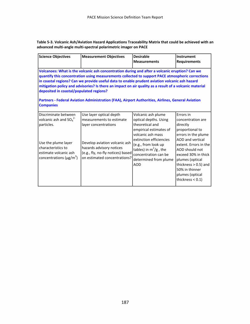
PACE Mission Science Definition Team Report
Table 5-3. Volcanic Ash/Aviation Hazard Applications Traceability Matrix that could be achieved with an advanced multi-angle multi-spectral polarimetric imager on PACE
Science Objectives Measurement Objectives Desirable Measurements
Instrument Requirements
Volcanoes: What is the volcanic ash concentration during and after a volcanic eruption? Can we quantify this concentration using measurements collected to support PACE atmospheric corrections in coastal regions? Can we provide useful data to enable prudent aviation volcanic ash hazard mitigation policy and advisories? Is there an impact on air quality as a result of a volcanic material deposited in coastal/populated regions?
Partners - Federal Aviation Administration (FAA), Airport Authorities, Airlines, General Aviation Companies
Discriminate between volcanic ash and SO4
2- particles.
Use the plume layer characteristics to estimate volcanic ash concentrations (µg/m3)
Use layer optical depth measurements to estimate layer concentrations
Develop aviation volcanic ash hazards advisory notices (e.g., fly, no-fly notices) based on estimated concentrations?
Volcanic ash plume optical depths. Using theoretical and empirical estimates of volcanic ash mass extinction efficiencies (e.g., from look up tables) in m2/g , the concentration can be determined from plume AOD
Errors in concentration are directly proportional to errors in the plume AOD and vertical extent. Errors in the AOD should not exceed 30% in thick plumes (optical thickness > 0.5) and 50% in thinner plumes (optical thickness < 0.1)
187
PACE Mission Science Definition Team Report
6 Conclusions Climate variability and human activity are having measurable and often negative impacts on marine ecosystems. In response to these challenges, NASA conceived the PACE mission to provide new information for understanding the living ocean and for improving forecasts of Earth system variability. The PACE mission will achieve these goals by making global ocean color measurements that are essential for understanding the carbon cycle and its interrelationship with climate change, and by expanding our understanding about ocean ecology and biogeochemistry. In this report we present ocean-related threshold science questions and measurements and mission requirements that are essential for the success of the PACE mission. The PACE mission also has a role in advancing atmospheric science. Therefore, this report also presents an independent atmosphere-related threshold science question and measurement requirements necessary to extend data records on aerosols and clouds. The SDT also concluded that the emphasis of the PACE mission is ocean ecology and biogeochemistry and that ocean science threshold measurement requirements cannot be traded for atmospheric threshold requirements. Below are abridged descriptions of the science questions and the instrument options required to address them.
1. To address threshold PACE ocean science questions the PACE mission must include:
• An accurately calibrated and well characterized ocean color instrument covering a spectral range of 350 to 800 nm at ~5 nm resolution, and including a short wavelength near-UV band (approximately centered around 350 nm), two NIR bands (one of which should be centered at 865 nm), and three SWIR bands (1240 nm, 1640 nm, and 2130 nm) for atmospheric corrections. All measurement bands must have a spatial resolution of 1 km2 (square pixel at nadir) with two-day global coverage. This instrument option is called OCI.
• A mission architecture that includes continual post-launch calibration (including lunar and vicarious calibration), frequent reprocessing of the entire data set, development and maintenance of algorithms, field validation, and process studies. The mission architecture should also include a robust satellite and integrated research program data and product distribution system that builds on the legacy systems built by the NASA Ocean Biology Processing Group (OBPG).
This OCI instrument and mission architecture option would address all the threshold ocean science questions that define the PACE mission, as well as the goal terrestrial ecology science questions.
All the mission options described below represent augmentations to the OCI concept that would add value to the mission. However, they will also add technical complexity
188
PACE Mission Science Definition Team Report
and cost. Adding these capabilities must not impact the capacity of the PACE mission to meet all of its threshold ocean science mission requirements.
2. To address the additional ocean science goals (i.e., to enhance research concerning threshold ocean science questions and enable research of coastal science goal questions), PACE mission measurement capabilities should exceed the threshold ocean science requirements to include:
• OCI with the following additions: (1) spatial resolution equal to or better than 500 m x 500 m to improve coverage of global coastal and estuarine areas; (2) a measurement band allowing assessment of aerosol heights, an SNR at 2130 nm of 100 or better, and an approach for assessing global NO2 and O3; (3) one-day global coverage, retrievals to solar zenith angles >75o, and equal pixel size across the measurement swath; and (4) hyperspectral (5 nm) coverage over 800-900 nm and 1 to 2 nm spectral subsampling capabilities. Sensor concepts that address all of these goals are preferred, but any of the various characteristics mentioned are desired as enhancements to the threshold mission concept. The instrument option addressing ocean science goals is referred to as OCI/OG.
3. To address the threshold atmosphere science question and achieve threshold (heritage) imager-based aerosol data records and a subset of cloud data records initiated during the Earth Observing System (EOS) era with the Moderate Resolution Imaging Spectroradiometer (MODIS) (and now continued with the Visible Infrared Imager Radiometer Suite [VIIRS]), the OCI would need to be augmented to include:
• The OCI with three additional SWIR bands (940 nm, 1378 nm, and 2250 nm) at 1 km2 spatial resolution. This instrument option is referred to as OCI+.
4. To provide advanced atmosphere products that address goal atmosphere science questions regarding the effect of aerosols on ocean productivity, aerosol direct radiative forcing, and improved atmospheric correction of ultraviolet (UV) products for ocean biology and biogeochemistry, the PACE mission would need to be augmented to include:
• The OCI plus a 3M imager. This option is called OCI-3M.
189
PACE Mission Science Definition Team Report
5. To provide advanced atmosphere products that address goal atmosphere science questions regarding how aerosols affect cloud properties, the PACE mission would need to include:
• The OCI+ instrument with 250 m spatial resolution in selected bands. While a 3M instrument is highly desirable, it is not essential. This option is called OCI/A.
6. To provide advanced atmosphere products that address goal atmosphere science questions regarding how clouds affect aerosol properties, as well as provide data continuity with the POLarization and Directionality of the Earth's Reflectances (POLDER) instrument and the NASA Terra Multi-angle Imaging SpectroRadiometer (MISR) instrument (though likely at reduced spatial resolution), the PACE mission would need to include:
• The OCI/A instrument with a 3M imager. This option is called OCI/A-3M.
Table 6-1 shows the science questions that are addressed by each instrument option. The table also offers a brief description of the instrument options to show their levels of complexity. All the mission options addressing the threshold atmosphere science question or the goal science questions are augmentations of the threshold ocean science mission described in this summary. Table 6-1 and the abridged descriptions above are not comprehensive, but are designed as a quick guide to the options that are most likely to drive the complexity and cost of the mission. A detailed list of goal measurement and mission requirements can be found in the body of this report.
190
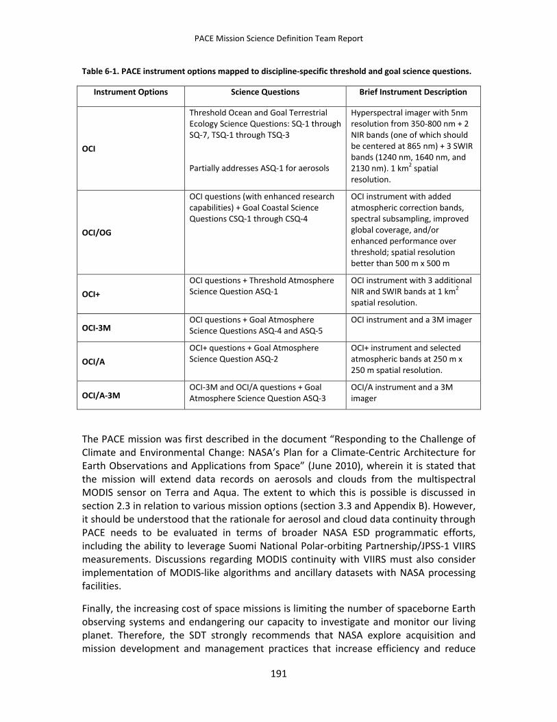
PACE Mission Science Definition Team Report
Table 6-1. PACE instrument options mapped to discipline-specific threshold and goal science questions.
Instrument Options Science Questions Brief Instrument Description
OCI
Threshold Ocean and Goal Terrestrial Ecology Science Questions: SQ-1 through SQ-7, TSQ-1 through TSQ-3
Partially addresses ASQ-1 for aerosols
Hyperspectral imager with 5nm resolution from 350-800 nm + 2 NIR bands (one of which should be centered at 865 nm) + 3 SWIR bands (1240 nm, 1640 nm, and 2130 nm). 1 km2 spatial resolution.
OCI/OG
OCI questions (with enhanced research capabilities) + Goal Coastal Science Questions CSQ-1 through CSQ-4
OCI instrument with added atmospheric correction bands, spectral subsampling, improved global coverage, and/or enhanced performance over threshold; spatial resolution better than 500 m x 500 m
OCI+ OCI questions + Threshold Atmosphere Science Question ASQ-1
OCI instrument with 3 additional NIR and SWIR bands at 1 km2 spatial resolution.
OCI-3M OCI questions + Goal Atmosphere Science Questions ASQ-4 and ASQ-5
OCI instrument and a 3M imager
OCI/A OCI+ questions + Goal Atmosphere Science Question ASQ-2
OCI+ instrument and selected atmospheric bands at 250 m x 250 m spatial resolution.
OCI/A-3M OCI-3M and OCI/A questions + Goal Atmosphere Science Question ASQ-3
OCI/A instrument and a 3M imager
The PACE mission was first described in the document “Responding to the Challenge of Climate and Environmental Change: NASA’s Plan for a Climate-Centric Architecture for Earth Observations and Applications from Space” (June 2010), wherein it is stated that the mission will extend data records on aerosols and clouds from the multispectral MODIS sensor on Terra and Aqua. The extent to which this is possible is discussed in section 2.3 in relation to various mission options (section 3.3 and Appendix B). However, it should be understood that the rationale for aerosol and cloud data continuity through PACE needs to be evaluated in terms of broader NASA ESD programmatic efforts, including the ability to leverage Suomi National Polar-orbiting Partnership/JPSS-1 VIIRS measurements. Discussions regarding MODIS continuity with VIIRS must also consider implementation of MODIS-like algorithms and ancillary datasets with NASA processing facilities.
Finally, the increasing cost of space missions is limiting the number of spaceborne Earth observing systems and endangering our capacity to investigate and monitor our living planet. Therefore, the SDT strongly recommends that NASA explore acquisition and mission development and management practices that increase efficiency and reduce
191

PACE Mission Science Definition Team Report
expenses. Early integration of instruments and spacecraft, as well as early selection of a launch vehicle, may reduce developmental costs. NASA should also consider the high costs of mission reviews and should strive to reduce management requirements that may increase cost without a concomitant increase in quality.
192
PACE Mission Science Definition Team Report
Appendix A Ocean Science Requirements Supplement: Parameter Ranges, Retrieval Sensitivities to Noise, and Signal-to-noise Requirements for Hyperspectral (5 nm) Bands
This appendix has four sections: (1) baseline and threshold retrieval ranges for optical, biological, and biogeochemical parameters related to ocean science questions; (2) atmospheric correction sensitivity to noise; (3) bio-optical algorithm retrieval sensitivity to noise; and (4) complete list of downlinked and archived PACE ocean science threshold bio-optical measurement bands, example NIR and SWIR atmospheric correction bands, and SNR requirements for all bands (see section 3.2 for requirements details). Parameter baseline and threshold ranges were assembled by the ACE ocean science team. The atmospheric correction analysis was conducted by Menghua Wang (NOAA/NESDIS) and Howard Gordon (U. of Miami). The bio-optical algorithm study was conducted by Stephane Maritorena (University of California/Santa Barbara) using inputs from the Wang and Gordon study.
A.1 Ocean Optical, Biological, and Biogeochemical Parameters Associated with each PACE science question is a set of geophysical parameters that must be measured in order to address the question. Remote sensing retrievals for each of these parameters require an algorithm that transforms the basic water-leaving radiances or remote sensing reflectances into an estimated value of that parameter over a range of values. In Table A-1 the various desired geophysical parameters are shown in the left-most column. For each parameter, the second and third columns indicate baseline and threshold ranges for the parameter, respectively. Here, the ‘baseline’ range represents the full desired retrieval range for a given parameter and is the range of values between the 1% and 99% region for the parameter frequency distribution. The ‘threshold’ range is the required retrieval range for a given parameter and represents the 5% to 95% region of the frequency distribution. Baseline and threshold values for the geophysical parameters were based on analyses of both field and historical satellite measurements. Specific information regarding these analyses for each parameter is provided in the right-most column of comments. It should be noted that values for each parameter have been measured that exceed even the baseline range, but these values are found under extreme and rare conditions and were not viewed as critical retrieval requirements for a satellite mission focused on global ocean properties.
193
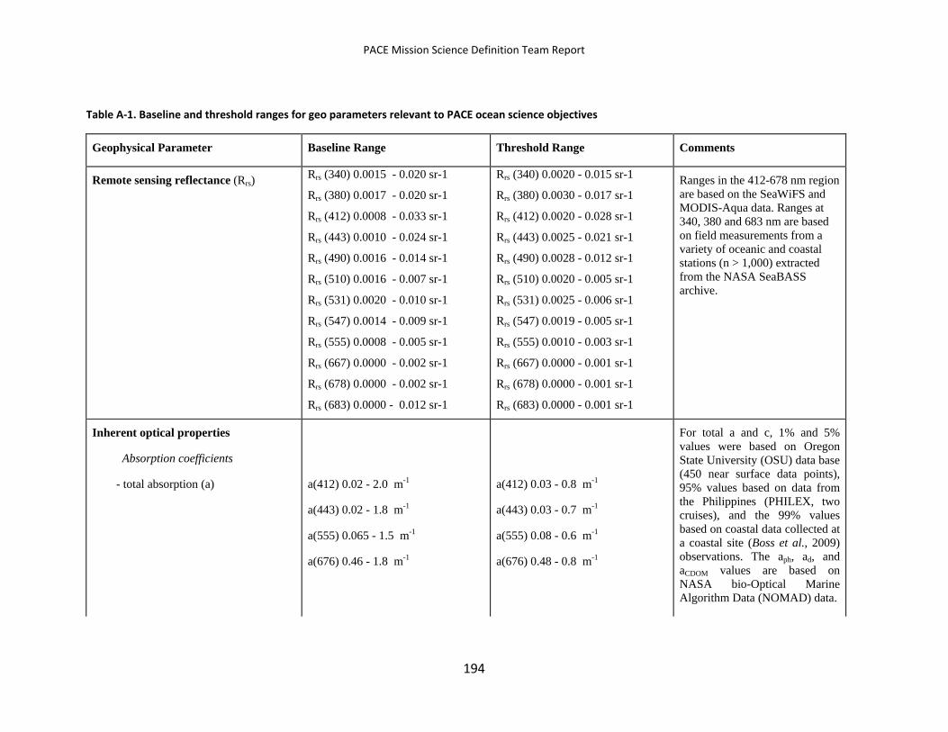
PACE Mission Science Definition Team Report
Table A-1. Baseline and threshold ranges for geo parameters relevant to PACE ocean science objectives
Geophysical Parameter Baseline Range Threshold Range Comments
Remote sensing reflectance (Rrs) Rrs (340) 0.0015 - 0.020 sr-1
Rrs (380) 0.0017 - 0.020 sr-1
Rrs (412) 0.0008 - 0.033 sr-1
Rrs (443) 0.0010 - 0.024 sr-1
Rrs (490) 0.0016 - 0.014 sr-1
Rrs (510) 0.0016 - 0.007 sr-1
Rrs (531) 0.0020 - 0.010 sr-1
Rrs (547) 0.0014 - 0.009 sr-1
Rrs (555) 0.0008 - 0.005 sr-1
Rrs (667) 0.0000 - 0.002 sr-1
Rrs (678) 0.0000 - 0.002 sr-1
Rrs (683) 0.0000 - 0.012 sr-1
Rrs (340) 0.0020 - 0.015 sr-1
Rrs (380) 0.0030 - 0.017 sr-1
Rrs (412) 0.0020 - 0.028 sr-1
Rrs (443) 0.0025 - 0.021 sr-1
Rrs (490) 0.0028 - 0.012 sr-1
Rrs (510) 0.0020 - 0.005 sr-1
Rrs (531) 0.0025 - 0.006 sr-1
Rrs (547) 0.0019 - 0.005 sr-1
Rrs (555) 0.0010 - 0.003 sr-1
Rrs (667) 0.0000 - 0.001 sr-1
Rrs (678) 0.0000 - 0.001 sr-1
Rrs (683) 0.0000 - 0.001 sr-1
Ranges in the 412-678 nm region are based on the SeaWiFS and MODIS-Aqua data. Ranges at 340, 380 and 683 nm are based on field measurements from a variety of oceanic and coastal stations (n > 1,000) extracted from the NASA SeaBASS archive.
Inherent optical properties
Absorption coefficients
- total absorption (a)
a(412) 0.02 - 2.0 m-1
a(443) 0.02 - 1.8 m-1
a(555) 0.065 - 1.5 m-1
a(676) 0.46 - 1.8 m-1
a(412) 0.03 - 0.8 m-1
a(443) 0.03 - 0.7 m-1
a(555) 0.08 - 0.6 m-1
a(676) 0.48 - 0.8 m-1
For total a and c, 1% and 5% values were based on Oregon State University (OSU) data base (450 near surface data points), 95% values based on data from the Philippines (PHILEX, two cruises), and the 99% values based on coastal data collected at a coastal site (Boss et al., 2009) observations. The aph, ad, and aCDOM values are based on NASA bio-Optical Marine Algorithm Data (NOMAD) data.
194
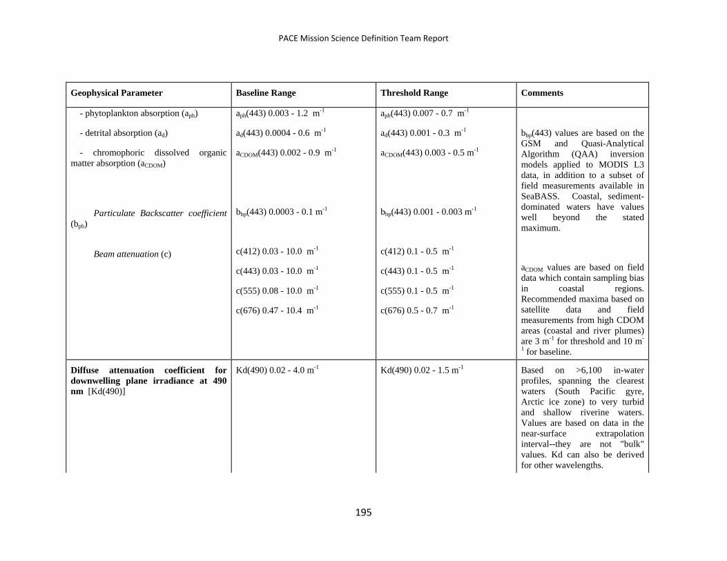
PACE Mission Science Definition Team Report
Geophysical Parameter Baseline Range Threshold Range Comments
- phytoplankton absorption (aph)
- detrital absorption (ad)
- chromophoric dissolved organic matter absorption (aCDOM)
Particulate Backscatter coefficient (bpb)
Beam attenuation (c)
aph(443) 0.003 - 1.2 m-1
ad(443) 0.0004 - 0.6 m-1
aCDOM(443) 0.002 - 0.9 m-1
bbp(443) 0.0003 - 0.1 m-1
c(412) 0.03 - 10.0 m-1
c(443) 0.03 - 10.0 m-1
c(555) 0.08 - 10.0 m-1
c(676) 0.47 - 10.4 m-1
aph(443) 0.007 - 0.7 m-1
ad(443) 0.001 - 0.3 m-1
aCDOM(443) 0.003 - 0.5 m-1
bbp(443) 0.001 - 0.003 m-1
c(412) 0.1 - 0.5 m-1
c(443) 0.1 - 0.5 m-1
c(555) 0.1 - 0.5 m-1
c(676) 0.5 - 0.7 m-1
bbp(443) values are based on the GSM and Quasi-Analytical Algorithm (QAA) inversion models applied to MODIS L3 data, in addition to a subset of field measurements available in SeaBASS. Coastal, sediment-dominated waters have values well beyond the stated maximum.
aCDOM values are based on field data which contain sampling bias in coastal regions. Recommended maxima based on satellite data and field measurements from high CDOM areas (coastal and river plumes) are 3 m-1 for threshold and 10 m-
1 for baseline.
Diffuse attenuation coefficient for downwelling plane irradiance at 490 nm [Kd(490)]
Kd(490) 0.02 - 4.0 m-1
Kd(490) 0.02 - 1.5 m-1 Based on >6,100 in-water profiles, spanning the clearest waters (South Pacific gyre, Arctic ice zone) to very turbid and shallow riverine waters. Values are based on data in the near-surface extrapolation interval--they are not "bulk" values. Kd can also be derived for other wavelengths.
195
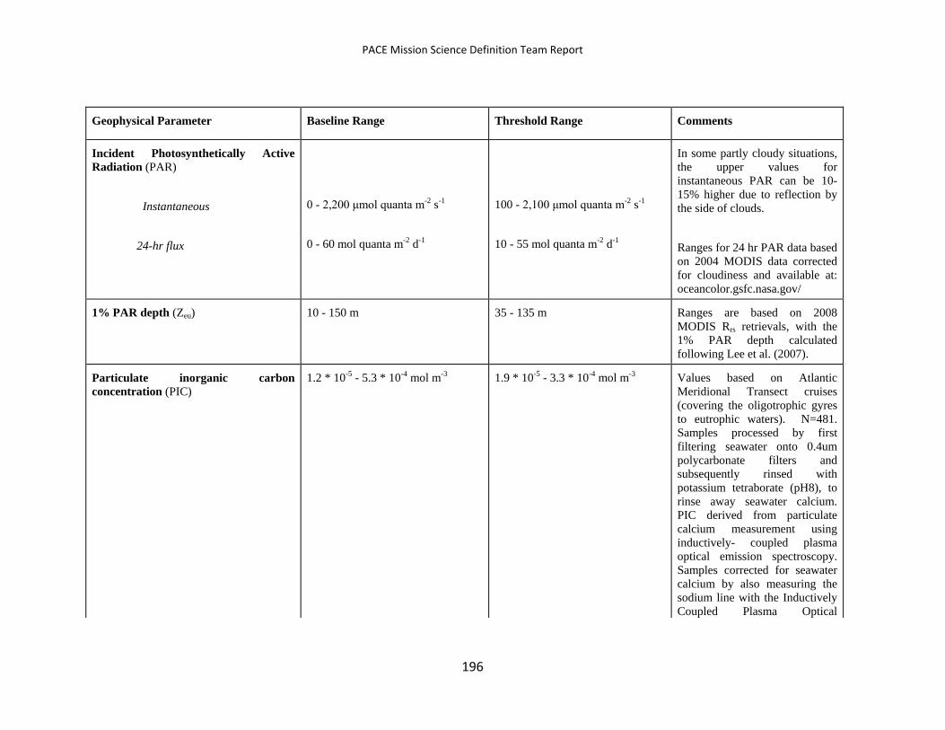
PACE Mission Science Definition Team Report
Geophysical Parameter Baseline Range Threshold Range Comments
Incident Photosynthetically Active Radiation (PAR)
Instantaneous
24-hr flux
0 - 2,200 μmol quanta m-2 s-1
0 - 60 mol quanta m-2 d-1
100 - 2,100 μmol quanta m-2 s-1
10 - 55 mol quanta m-2 d-1
In some partly cloudy situations, the upper values for instantaneous PAR can be 10-15% higher due to reflection by the side of clouds.
Ranges for 24 hr PAR data based on 2004 MODIS data corrected for cloudiness and available at: oceancolor.gsfc.nasa.gov/
1% PAR depth (Zeu) 10 - 150 m 35 - 135 m Ranges are based on 2008 MODIS Rrs retrievals, with the 1% PAR depth calculated following Lee et al. (2007).
Particulate inorganic carbon concentration (PIC)
1.2 * 10-5 - 5.3 * 10-4 mol m-3 1.9 * 10-5 - 3.3 * 10-4 mol m-3 Values based on Atlantic Meridional Transect cruises (covering the oligotrophic gyres to eutrophic waters). N=481. Samples processed by first filtering seawater onto 0.4um polycarbonate filters and subsequently rinsed with potassium tetraborate (pH8), to rinse away seawater calcium. PIC derived from particulate calcium measurement using inductively- coupled plasma optical emission spectroscopy. Samples corrected for seawater calcium by also measuring the sodium line with the Inductively Coupled Plasma Optical
196
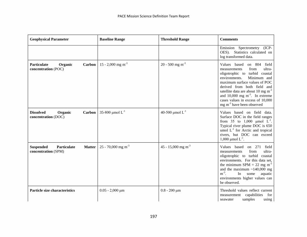
PACE Mission Science Definition Team Report
Geophysical Parameter Baseline Range Threshold Range Comments
Emission Spectrometry (ICP-OES). Statistics calculated on log transformed data.
Particulate Organic Carbon concentration (POC)
15 - 2,000 mg m-3 20 - 500 mg m-3 Values based on 804 field measurements from ultra- oligotrophic to turbid coastal environments. Minimum and maximum surface values of POC derived from both field and satellite data are about 10 mg m-3 and 10,000 mg m-3. In extreme cases values in excess of 10,000 mg m-3 have been observed
Dissolved Organic Carbon concentration (DOC)
35-800 μmol L-1
40-500 μmol L-1 Values based on field data. Surface DOC in the field ranges from 35 to 1,000 μmol L-1. Typical river plume DOC is 650 umol L-1 for Arctic and tropical rivers, but DOC can exceed 1,000 μmol L-1.
Suspended Particulate Matter concentration (SPM)
25 - 70,000 mg m-3 45 - 15,000 mg m-3 Values based on 271 field measurements from ultra- oligotrophic to turbid coastal environments. For this data set, the minimum SPM = 22 mg m-3 and the maximum ~140,000 mg m-3. In some aquatic environments higher values can be observed.
Particle size characteristics 0.05 - 2,000 μm 0.8 - 200 μm Threshold values reflect current measurement capabilities for seawater samples using
197
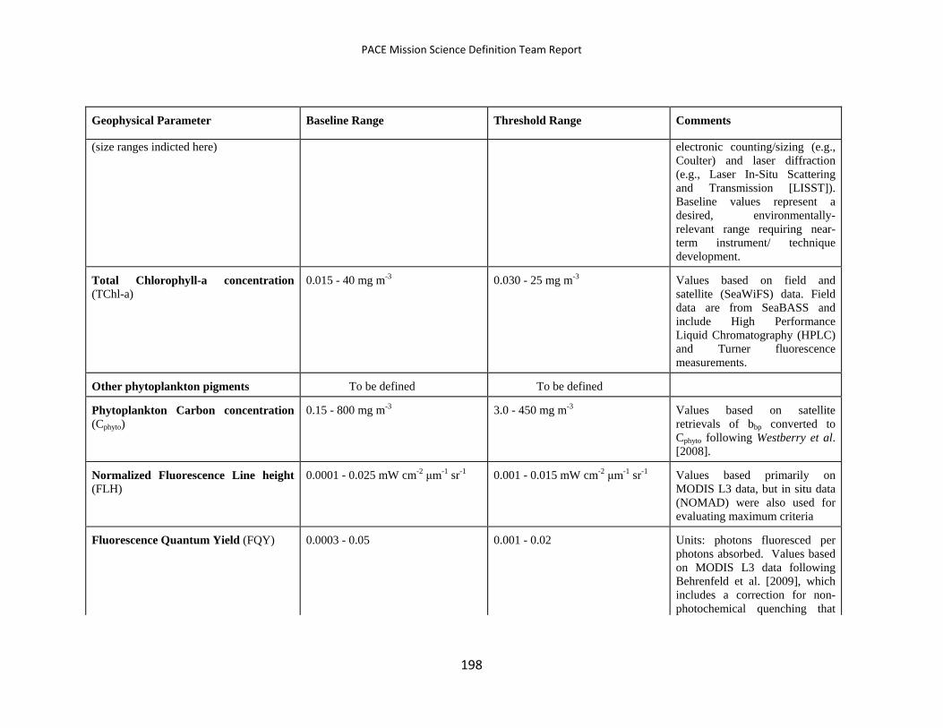
PACE Mission Science Definition Team Report
Geophysical Parameter Baseline Range Threshold Range Comments
(size ranges indicted here)
electronic counting/sizing (e.g., Coulter) and laser diffraction (e.g., Laser In-Situ Scattering and Transmission [LISST]). Baseline values represent a desired, environmentally-relevant range requiring near-term instrument/ technique development.
Total Chlorophyll-a concentration (TChl-a)
0.015 - 40 mg m-3 0.030 - 25 mg m-3 Values based on field and satellite (SeaWiFS) data. Field data are from SeaBASS and include High Performance Liquid Chromatography (HPLC) and Turner fluorescence measurements.
Other phytoplankton pigments To be defined To be defined
Phytoplankton Carbon concentration (Cphyto)
0.15 - 800 mg m-3
3.0 - 450 mg m-3
Values based on satellite retrievals of bbp converted to Cphyto following Westberry et al. [2008].
Normalized Fluorescence Line height (FLH)
0.0001 - 0.025 mW cm-2 μm-1 sr-1 0.001 - 0.015 mW cm-2 μm-1 sr-1 Values based primarily on MODIS L3 data, but in situ data (NOMAD) were also used for evaluating maximum criteria
Fluorescence Quantum Yield (FQY) 0.0003 - 0.05 0.001 - 0.02 Units: photons fluoresced per photons absorbed. Values based on MODIS L3 data following Behrenfeld et al. [2009], which includes a correction for non-photochemical quenching that
198
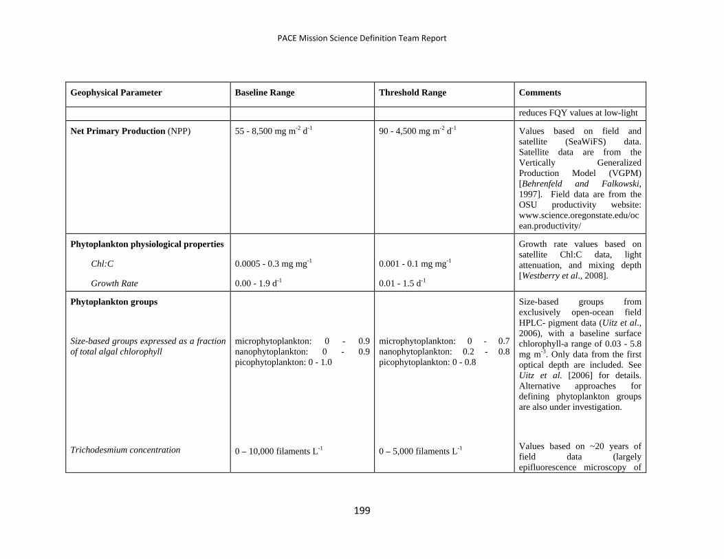
PACE Mission Science Definition Team Report
Geophysical Parameter Baseline Range Threshold Range Comments
reduces FQY values at low-light
Net Primary Production (NPP)
55 - 8,500 mg m-2 d-1 90 - 4,500 mg m-2 d-1
Values based on field and satellite (SeaWiFS) data. Satellite data are from the Vertically Generalized Production Model (VGPM) [Behrenfeld and Falkowski, 1997]. Field data are from the OSU productivity website: www.science.oregonstate.edu/ocean.productivity/
Phytoplankton physiological properties
Chl:C
Growth Rate
0.0005 - 0.3 mg mg-1
0.00 - 1.9 d-1
0.001 - 0.1 mg mg-1
0.01 - 1.5 d-1
Growth rate values based on satellite Chl:C data, light attenuation, and mixing depth [Westberry et al., 2008].
Phytoplankton groups
Size-based groups expressed as a fraction of total algal chlorophyll
Trichodesmium concentration
microphytoplankton: 0 - 0.9 nanophytoplankton: 0 - 0.9 picophytoplankton: 0 - 1.0
0 – 10,000 filaments L-1
microphytoplankton: 0 - 0.7 nanophytoplankton: 0.2 - 0.8 picophytoplankton: 0 - 0.8
0 – 5,000 filaments L-1
Size-based groups from exclusively open-ocean field HPLC- pigment data (Uitz et al., 2006), with a baseline surface chlorophyll-a range of 0.03 - 5.8 mg m-3. Only data from the first optical depth are included. See Uitz et al. [2006] for details. Alternative approaches for defining phytoplankton groups are also under investigation.
Values based on ~20 years of field data (largely epifluorescence microscopy of
199
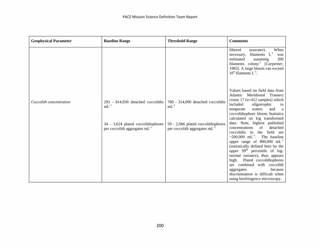
PACE Mission Science Definition Team Report
Geophysical Parameter Baseline Range Threshold Range Comments
Coccolith concentration
293 - 814,930 detached coccoliths mL-1
34 - 3,624 plated coccolithophores per coccolith aggregates mL-1
760 - 314,000 detached coccoliths mL-1
59 - 2,066 plated coccolithophores per coccolith aggregates mL-1
filtered seawater). When necessary, filaments L-1 was estimated assuming 200 filaments colony-1 [Carpenter, 1983]. A large bloom can exceed 106 filaments L-1.
Values based on field data from Atlantic Meridional Transect cruise 17 (n=412 samples) which included oligotrophic to temperate waters and a coccolithophore bloom Statistics calculated on log transformed data. Note, highest published concentrations of detached coccoliths in the field are ~500,000 mL-1. The baseline upper range of 800,000 mL-1 (statistically defined here by the upper 99th percentile of log-normal variance), thus, appears high. Plated coccolithophores are combined with coccolith aggregates because discrimination is difficult when using birefringence microscopy.
200
PACE Mission Science Definition Team Report
A.2 Simulations for the NIR and SWIR SNR Requirements for Atmospheric Corrections
Atmospheric correction for ocean color product is extremely sensitive to sensor spectral band calibration errors, as well as to radiometric noise. This is due to the considerably low radiance from the ocean compared to the sensor-measured top-of-atmosphere (TOA) radiance. The sensor spectral band radiometric performance can be characterized by the signal to noise ratio (SNR). To understand the radiometric noise effects on the derived normalized water-leaving reflectance spectra, simulations of atmospheric correction, using the two near-infrared (NIR) bands (765 and 865 nm) and various combinations of the short-wave infrared (SWIR) bands (1240, 1640, and 2130 nm), have been carried out for several levels of sensor noise.
A.2.1 Noise Model A Gaussian distribution (with mean value = 0) is used for the noise simulations. The standard deviation (STD) of the Gaussian distribution is the radiance noise level (i.e., related to the SNR values). The simulated reflectance noise is then added into the TOA reflectance at various NIR and SWIR bands that are used for making atmospheric correction. Eight noise levels are generated, corresponding to eight SNR values of 25, 50, 100, 200, 400, 600, 800, and 1000. It is noted that the reflectance noise is only added into the bands that are used for atmospheric correction (e.g., two NIR bands), and UV and visible bands are noise-free in all simulations discussed in this subsection. The reflectance noises are spectrally incoherent.
A.2.2 Atmospheric Correction Atmospheric correction simulations using two NIR bands [Gordon and Wang, 1994] and various SWIR bands [Wang, 2007] have been carried out, including reflectance noise levels for the corresponding NIR and SWIR bands. Specifically, simulations were carried out for a typical Maritime aerosol model (M80) and a Tropospheric model (T80), where the T80 model is actually the M80 model without the large size fraction, for aerosol optical thicknesses (at 865 nm) of 0.05, 0.1, 0.2, and 0.3. The M80 and T80 aerosol models were not used in the aerosol lookup tables for atmospheric correction [Gordon and Wang, 1994; Wang, 2007]. Simulations were performed for a case with solar-zenith angle of 60°, sensor-zenith angle of 45°, and relative azimuth angle of 90°.
201
PACE Mission Science Definition Team Report
A.2.3 SNR Simulations For each case, atmospheric correction for 5000 noise realizations with a given SNR value was carried out. For example, for a case with aerosol optical thickness (AOT) at 865 nm of 0.1, 5000 reflectance noise samples (with a given SNR value) were generated and added into the TOA NIR (765 and 865 nm) reflectance values. The NIR atmospheric correction [Gordon and Wang, 1994] was then performed 5000 times to generate the corresponding normalized water-leaving reflectance spectra error. The same procedure was carried out for all four AOTs, and also for the SWIR algorithm [Wang, 2007]. In the SWIR atmospheric correction, however, the Gaussian noise was of course added into the SWIR bands (error free for UV to NIR bands). This produces the uncertainty in the derived normalized water-leaving reflectance from the UV to the red (or NIR in the case of the SWIR bands). In effect, the simulated uncertainty includes errors from both the atmospheric correction algorithm and the added Gaussian noise in the NIR or SWIR bands. The reflectance uncertainty spectra (from UV to red) are then used for the bio-optical model sensitivity analysis by Stephane Maritorena.
A.2.4 Example Results Figure A-1 provides sample results in the reflectance uncertainty spectra (UV to red or UV to NIR) with simulations from atmospheric correction algorithm using the NIR or SWIR bands. The error in the normalized water-leaving reflectance, [ρw(λ)]N, is actually the standard deviation of the derived uncertainty in [ρw(λ)]N over the 5000 Gaussian noise realizations; i.e., each point in the plot was derived from 5000 simulations, ([ρw(λ)]N errors were first obtained with these 5000 simulations, and then the STD error was derived). The STD error was computed assuming that the mean value = 0 (i.e., error free). Figure A-1(a) and (b) are results for the NIR atmospheric correction algorithm (using 765 and 865 nm) with the M80 and T80 aerosol models, respectively, while Figure A-1(c) and (d) are results for the M80 and T80 aerosols using the SWIR atmospheric correction algorithm (with bands of 1240 and 1640 nm) for various SNR values. Note that for the SWIR results (Figure A-1(c) and (d)), errors in [ρw(λ)]N for two NIR bands are also included. Results in Figure A-1 show that, as SNR value increases (or noise decreases), error in [ρw(λ)]N decreases (as expected), and it reaches the inherent algorithm error [Gordon and Wang, 1994; Wang, 2007].
202
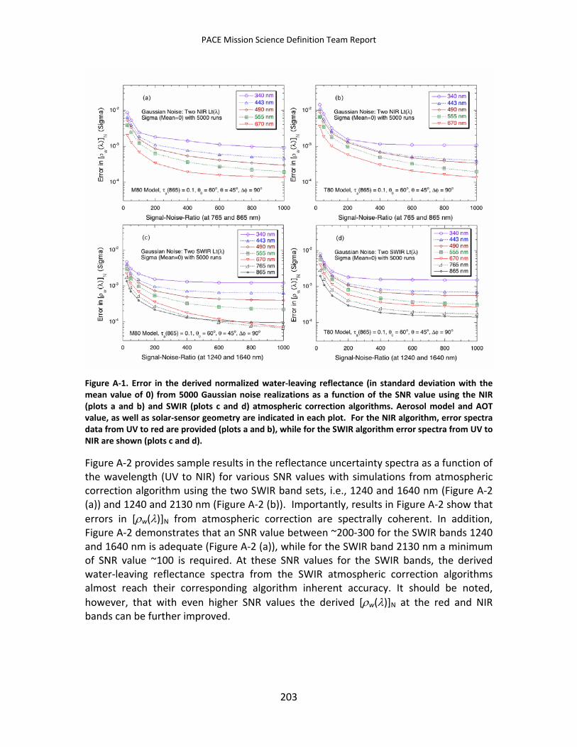
PACE Mission Science Definition Team Report
Figure A-1. Error in the derived normalized water-leaving reflectance (in standard deviation with the mean value of 0) from 5000 Gaussian noise realizations as a function of the SNR value using the NIR (plots a and b) and SWIR (plots c and d) atmospheric correction algorithms. Aerosol model and AOT value, as well as solar-sensor geometry are indicated in each plot. For the NIR algorithm, error spectra data from UV to red are provided (plots a and b), while for the SWIR algorithm error spectra from UV to NIR are shown (plots c and d).
Figure A-2 provides sample results in the reflectance uncertainty spectra as a function of the wavelength (UV to NIR) for various SNR values with simulations from atmospheric correction algorithm using the two SWIR band sets, i.e., 1240 and 1640 nm (Figure A-2 (a)) and 1240 and 2130 nm (Figure A-2 (b)). Importantly, results in Figure A-2 show that errors in [ρw(λ)]N from atmospheric correction are spectrally coherent. In addition, Figure A-2 demonstrates that an SNR value between ~200-300 for the SWIR bands 1240 and 1640 nm is adequate (Figure A-2 (a)), while for the SWIR band 2130 nm a minimum of SNR value ~100 is required. At these SNR values for the SWIR bands, the derived water-leaving reflectance spectra from the SWIR atmospheric correction algorithms almost reach their corresponding algorithm inherent accuracy. It should be noted, however, that with even higher SNR values the derived [ρw(λ)]N at the red and NIR bands can be further improved.
203
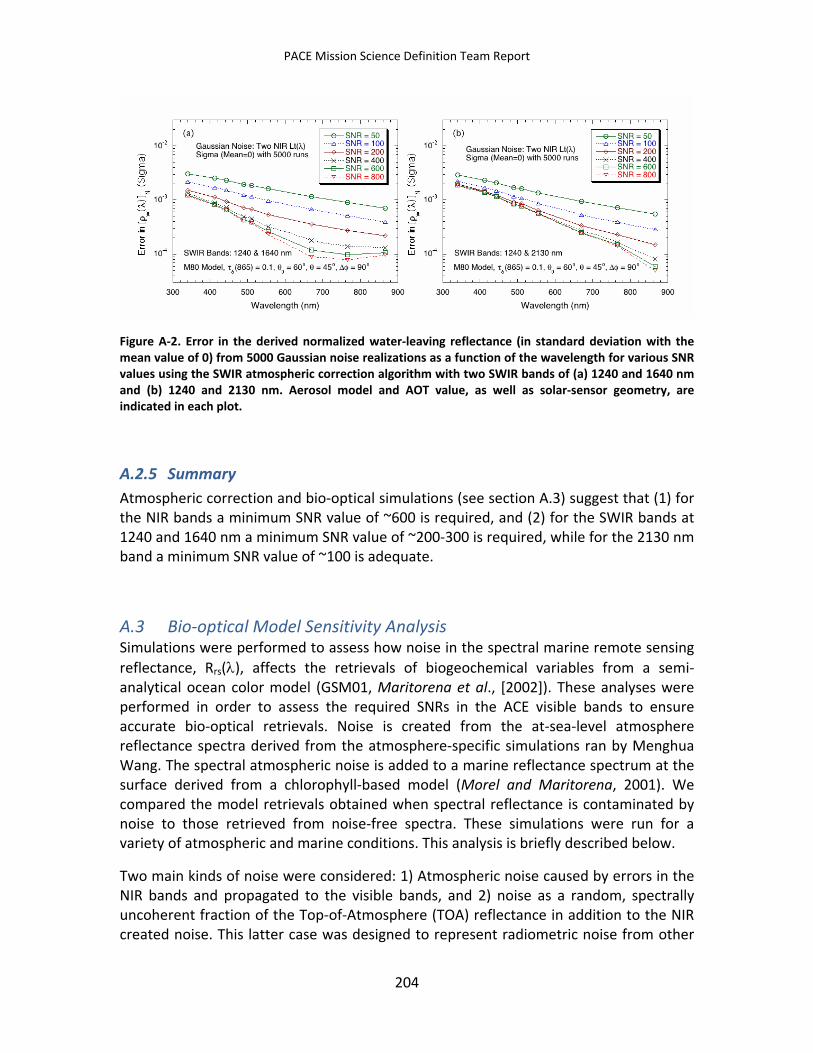
PACE Mission Science Definition Team Report
Figure A-2. Error in the derived normalized water-leaving reflectance (in standard deviation with the mean value of 0) from 5000 Gaussian noise realizations as a function of the wavelength for various SNR values using the SWIR atmospheric correction algorithm with two SWIR bands of (a) 1240 and 1640 nm and (b) 1240 and 2130 nm. Aerosol model and AOT value, as well as solar-sensor geometry, are indicated in each plot.
A.2.5 Summary Atmospheric correction and bio-optical simulations (see section A.3) suggest that (1) for the NIR bands a minimum SNR value of ~600 is required, and (2) for the SWIR bands at 1240 and 1640 nm a minimum SNR value of ~200-300 is required, while for the 2130 nm band a minimum SNR value of ~100 is adequate.
A.3 Bio-optical Model Sensitivity Analysis Simulations were performed to assess how noise in the spectral marine remote sensing reflectance, Rrs(λ), affects the retrievals of biogeochemical variables from a semi-analytical ocean color model (GSM01, Maritorena et al., [2002]). These analyses were performed in order to assess the required SNRs in the ACE visible bands to ensure accurate bio-optical retrievals. Noise is created from the at-sea-level atmosphere reflectance spectra derived from the atmosphere-specific simulations ran by Menghua Wang. The spectral atmospheric noise is added to a marine reflectance spectrum at the surface derived from a chlorophyll-based model (Morel and Maritorena, 2001). We compared the model retrievals obtained when spectral reflectance is contaminated by noise to those retrieved from noise-free spectra. These simulations were run for a variety of atmospheric and marine conditions. This analysis is briefly described below.
Two main kinds of noise were considered: 1) Atmospheric noise caused by errors in the NIR bands and propagated to the visible bands, and 2) noise as a random, spectrally uncoherent fraction of the Top-of-Atmosphere (TOA) reflectance in addition to the NIR created noise. This latter case was designed to represent radiometric noise from other
204
PACE Mission Science Definition Team Report
sources than the NIR bands (e.g., calibration). These two cases will be referred to as "NIR" and "radiometric" errors, respectively.
In all runs, the "pure" marine Rrs signal ( = no noise) is generated from the MM01 model [Morel and Maritorena, 2001] for ten chlorophyll concentration (Chl) values in the 0.02-5 mg/m3 range (400-700 nm every 5 nm). The GSM01 retrievals from the inversion of these "no noise" spectra are the reference to which the "noisy" NIR and radiometric cases are compared.
For the "NIR" errors case, the at-sea-level reflectance spectra caused by errors in the NIR bands (from Menghua Wang) are converted to Rrs, Rrs _NIR(λ), and added to a MM01 marine spectrum, Rrs_MM01(λ, Chl), so
Rrs(λ, ocean) = Rrs_MM01(λ, Chl)+ Rrs_NIR(λ)
The resulting spectrum, Rrs(λ, ocean), is then inverted in GSM. The three GSM retrievals (Chl, Chromophoric Detrital Material [CDM], bbp) are then compared to the "no noise" case for 5000 spectra for each combination of SNR (eight values), AOT(865) and atmospheric model (two models) and marine Rrs(λ) (ten spectra). The comparisons are expressed in terms of the % rms for each of the GSM01 product and at each Chl level used to generate the marine Rrs. The % rms is defined as rms*100/reference (reference = retrieval in the no noise case).
For the "radiometric" errors case, a random, Gaussian, spectrally uncoherent fraction of a TOA signal is added to the marine spectra created, similarly to what is described in the "NIR" case above. First, TOA signals are constructed for a black ocean with the M80 and T80 models, AOT(865) = 0.1 and for solar, sensor, and relative azimuth angles of 60, 45, and 90 degrees, respectively. The ocean contribution to the TOA signal is calculated as a MM01 reflectance spectrum transmitted through the atmosphere (with transmittance values matching the atmospheric model and geometry and AOT(865) of 0.05, 0.1, 0.2, and 0.3) and is added to the atmospheric TOA component (converted to Rrs units; Rrs_TOA(λ)). The fraction of the TOA signal that is added to the marine spectrum created, as in the NIR cases, is determined through the generation of random Gaussian numbers with a mean of 0 and a standard-deviation of 1/SNR(visible) with SNR(visible) set to 10, 20, 40, 100, 200, 400, 800, 1000 and 2000. Then, each wavelength of the TOA spectrum is multiplied by a unique random number (rn) and that fraction of the TOA spectrum is added to the other components of the marine signal. This is done independently for each of the 5000 spectra corresponding to each SNR(NIR)/AOT(865)/atmospheric model combination used in the atmosphere simulations. In summary, in the "radiometric" errors case, the at-sea-level Rrs is generated as:
Rrs(λ, ocean) = Rrs_MM01(λ, Chl)+ Rrs_NIR(λ) + (Rrs_TOA(λ) * rn(λ, SNR(visible))
By looking at how much the retrievals from the noisy reflectance spectra depart from those derived without addition of noise, it is possible to assess the SNR(visible) value
205
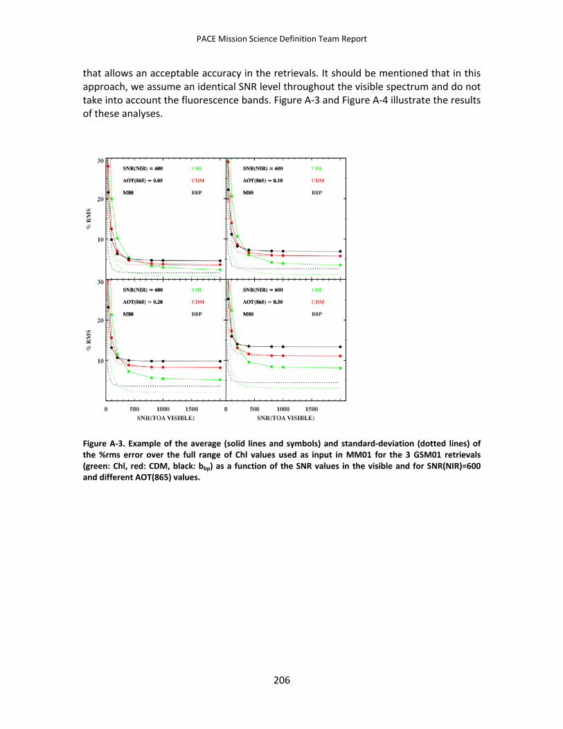
PACE Mission Science Definition Team Report
that allows an acceptable accuracy in the retrievals. It should be mentioned that in this approach, we assume an identical SNR level throughout the visible spectrum and do not take into account the fluorescence bands. Figure A-3 and Figure A-4 illustrate the results of these analyses.
Figure A-3. Example of the average (solid lines and symbols) and standard-deviation (dotted lines) of the %rms error over the full range of Chl values used as input in MM01 for the 3 GSM01 retrievals (green: Chl, red: CDM, black: bbp) as a function of the SNR values in the visible and for SNR(NIR)=600 and different AOT(865) values.
206
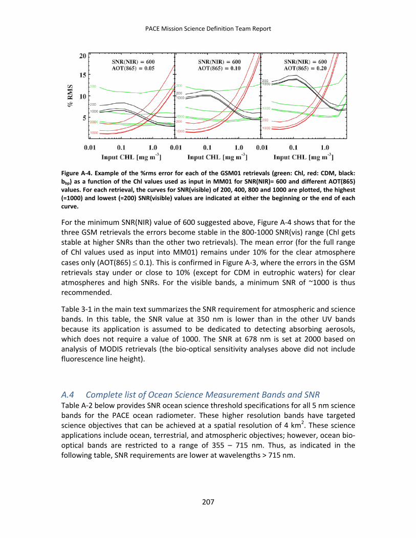
PACE Mission Science Definition Team Report
Figure A-4. Example of the %rms error for each of the GSM01 retrievals (green: Chl, red: CDM, black: bbp) as a function of the Chl values used as input in MM01 for SNR(NIR)= 600 and different AOT(865) values. For each retrieval, the curves for SNR(visible) of 200, 400, 800 and 1000 are plotted, the highest (=1000) and lowest (=200) SNR(visible) values are indicated at either the beginning or the end of each curve.
For the minimum SNR(NIR) value of 600 suggested above, Figure A-4 shows that for the three GSM retrievals the errors become stable in the 800-1000 SNR(vis) range (Chl gets stable at higher SNRs than the other two retrievals). The mean error (for the full range of Chl values used as input into MM01) remains under 10% for the clear atmosphere cases only (AOT(865) ≤ 0.1). This is confirmed in Figure A-3, where the errors in the GSM retrievals stay under or close to 10% (except for CDM in eutrophic waters) for clear atmospheres and high SNRs. For the visible bands, a minimum SNR of ~1000 is thus recommended.
Table 3-1 in the main text summarizes the SNR requirement for atmospheric and science bands. In this table, the SNR value at 350 nm is lower than in the other UV bands because its application is assumed to be dedicated to detecting absorbing aerosols, which does not require a value of 1000. The SNR at 678 nm is set at 2000 based on analysis of MODIS retrievals (the bio-optical sensitivity analyses above did not include fluorescence line height).
A.4 Complete list of Ocean Science Measurement Bands and SNR Table A-2 below provides SNR ocean science threshold specifications for all 5 nm science bands for the PACE ocean radiometer. These higher resolution bands have targeted science objectives that can be achieved at a spatial resolution of 4 km2. These science applications include ocean, terrestrial, and atmospheric objectives; however, ocean bio-optical bands are restricted to a range of 355 – 715 nm. Thus, as indicated in the following table, SNR requirements are lower at wavelengths > 715 nm.
207
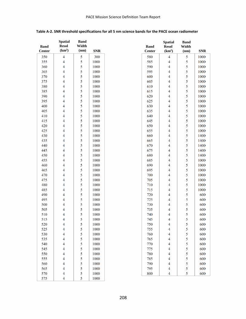
PACE Mission Science Definition Team Report
Table A-2. SNR threshold specifications for all 5 nm science bands for the PACE ocean radiometer
SpatialResol (km2)
BandWidth (nm) SNR
BandCenter SNR
BandCenter
SpatialResol (km2)
BandWidth (nm)
208
PACE Mission Science Definition Team Report
Appendix B Rationale for Atmosphere Team Measurement Requirements
This appendix contains supplementary figures and other information providing further rationale for the key augmented OCI imager (OCI+) cloud measurement requirements and related retrieval capabilities discussed in sections 3.3 and 2.3, respectively. The science associated with the below augmentations have been noted for further Phase A studies (section 2.3.2.5).
B.1 Spectral Augmentation
B.1.1 Oxygen A-band and 940 nm Water Vapor Channels Section 2.3.2.1.3 discussed the use of various absorption bands in the VIS/NIR part of the spectrum that can be used to infer cloud height from an OCI imager (or more specifically, mid-height for vertically extensive clouds). The most important band is expected to the O2 A-band (with 5 nm resolution, Table 3-4) with supplemental information from the 940 nm water vapor band. In addition, both bands provide information on multilayer scene detection. Finally, if cloud height is known sufficiently from the A-band, the 940 nm band can be used to retrieve above-cloud water vapor that can be used to correct for water vapor absorption in other cloud and/or aerosol channels. The height information obtained from both A-band and NIR water vapor absorption measurements is expected to correspond to the mid-cloud pressure (MCP) as discussed in section 2.3.2.1.3.
Figure B-1 (a) shows the round-trip path absorption for all O2 and H2O absorption bands discussed in section 2.3.2 as a function of altitude for an overhead sun and nadir view geometry. The bandpasses used for calculating oxygen and water vapor band absorption are consistent with the A-band and 940 nm instrument measurement requirements of Table 3-4. The O2 A-band has significant path absorption (~60% for a 4 km level) and its derivative (see panel (b)) shows nearly uniform height sensitivity throughout the troposphere. In contrast, the 940 nm band has peak sensitivity in the lower troposphere, as expected, with significantly more absorption for levels below 4 km (mid-latitude summer ocean profile). This is expected to be particularly useful given the PACE mission’s emphasis on low clouds. However, cloud height information content from the 940 nm band will require model analyses and this error source will need to be considered in a combined O2 and water vapor algorithm.
209
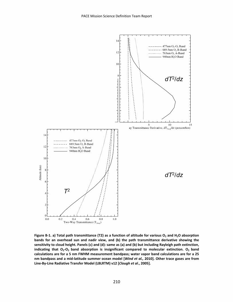
PACE Mission Science Definition Team Report
Figure B-1. a) Total path transmittance (T2) as a function of altitude for various O2 and H2O absorption bands for an overhead sun and nadir view, and (b) the path transmittance derivative showing the sensitivity to cloud height. Panels (c) and (d): same as (a) and (b) but including Rayleigh path extinction, indicating that O2-O2 band absorption is insignificant compared to molecular extinction. O2 band calculations are for a 5 nm FWHM measurement bandpass; water vapor band calculations are for a 25 nm bandpass and a mid-latitude summer ocean model [Wind et al., 2010]. Other trace gases are from Line-By-Line Radiative Transfer Model (LBLRTM) v12 [Clough et al., 2005].
210
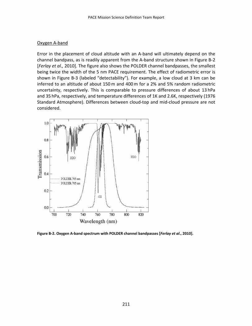
PACE Mission Science Definition Team Report
Oxygen A-band
Error in the placement of cloud altitude with an A-band will ultimately depend on the channel bandpass, as is readily apparent from the A-band structure shown in Figure B-2 [Ferlay et al., 2010]. The figure also shows the POLDER channel bandpasses, the smallest being twice the width of the 5 nm PACE requirement. The effect of radiometric error is shown in Figure B-3 (labeled “detectability”). For example, a low cloud at 3 km can be inferred to an altitude of about 150 m and 400 m for a 2% and 5% random radiometric uncertainty, respectively. This is comparable to pressure differences of about 13 hPa and 35 hPa, respectively, and temperature differences of 1K and 2.6K, respectively (1976 Standard Atmosphere). Differences between cloud-top and mid-cloud pressure are not considered.
Figure B-2. Oxygen A-band spectrum with POLDER channel bandpasses [Ferlay et al., 2010].
211
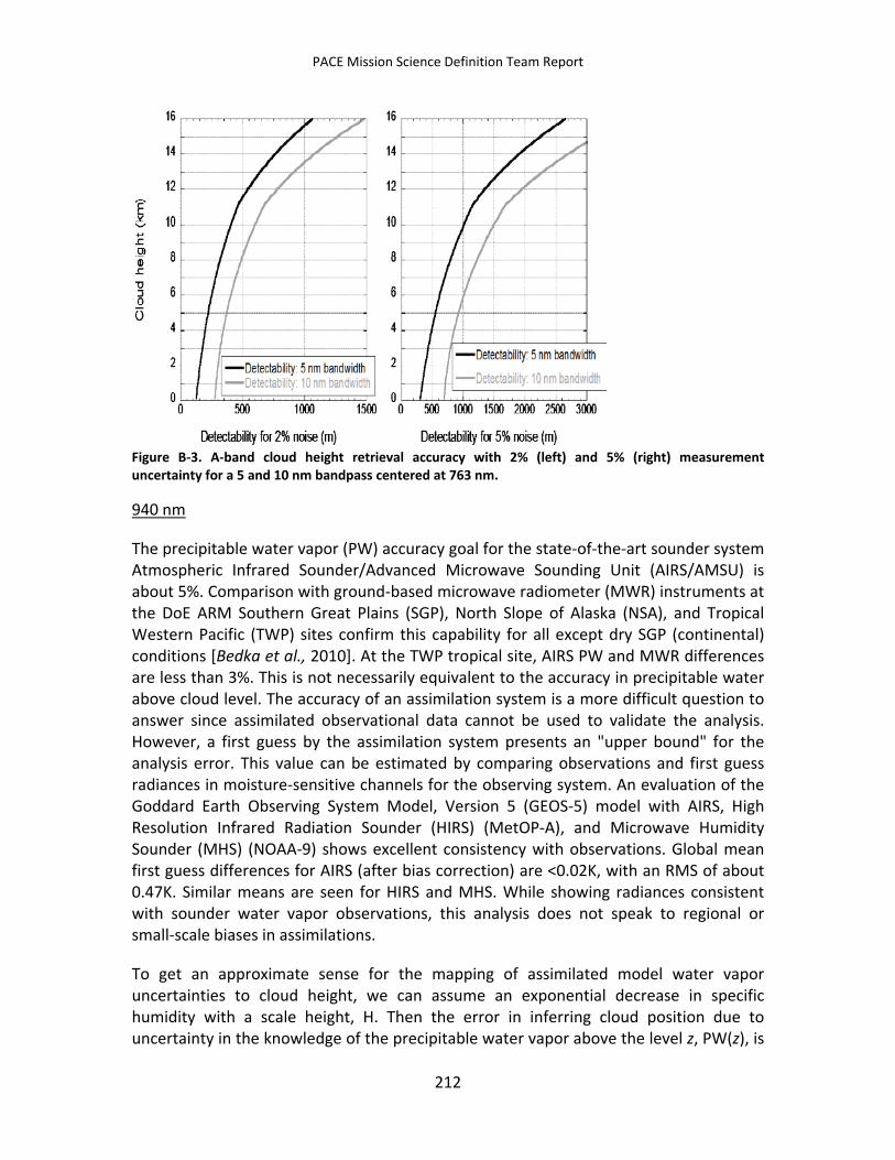
PACE Mission Science Definition Team Report
Figure B-3. A-band cloud height retrieval accuracy with 2% (left) and 5% (right) measurement uncertainty for a 5 and 10 nm bandpass centered at 763 nm.
940 nm
The precipitable water vapor (PW) accuracy goal for the state-of-the-art sounder system Atmospheric Infrared Sounder/Advanced Microwave Sounding Unit (AIRS/AMSU) is about 5%. Comparison with ground-based microwave radiometer (MWR) instruments at the DoE ARM Southern Great Plains (SGP), North Slope of Alaska (NSA), and Tropical Western Pacific (TWP) sites confirm this capability for all except dry SGP (continental) conditions [Bedka et al., 2010]. At the TWP tropical site, AIRS PW and MWR differences are less than 3%. This is not necessarily equivalent to the accuracy in precipitable water above cloud level. The accuracy of an assimilation system is a more difficult question to answer since assimilated observational data cannot be used to validate the analysis. However, a first guess by the assimilation system presents an "upper bound" for the analysis error. This value can be estimated by comparing observations and first guess radiances in moisture-sensitive channels for the observing system. An evaluation of the Goddard Earth Observing System Model, Version 5 (GEOS-5) model with AIRS, High Resolution Infrared Radiation Sounder (HIRS) (MetOP-A), and Microwave Humidity Sounder (MHS) (NOAA-9) shows excellent consistency with observations. Global mean first guess differences for AIRS (after bias correction) are <0.02K, with an RMS of about 0.47K. Similar means are seen for HIRS and MHS. While showing radiances consistent with sounder water vapor observations, this analysis does not speak to regional or small-scale biases in assimilations.
To get an approximate sense for the mapping of assimilated model water vapor uncertainties to cloud height, we can assume an exponential decrease in specific humidity with a scale height, H. Then the error in inferring cloud position due to uncertainty in the knowledge of the precipitable water vapor above the level z, PW(z), is
212
PACE Mission Science Definition Team Report
approximated as ∆z ≈ H ∆PW(z)/PW(z). For example, a scale height of 2 km and a 5% error in PW(z) results in an error of 100 m in the location of the cloud (assuming no measurement uncertainty), and 200 m for a more conservative 10% PW(z) error. For comparison with Figure B-3, a 150 m and 400 m uncertainty in O2 A-band derived cloud height (cloud at 2 km with 2% and 5% radiometric uncertainty, respectively) is equivalent to a PW(z) relative of error of 7.5% and 20%, respectively.
Including the effect of measurement uncertainty gives ∆z ≈ H ∆PW(z)/PW(z) + σm/(dT2/dz), where an example of the latter derivative function is given in Figure B-1. The NIR vapor path absorption would nominally be derived from the 940 nm to 865 nm reflectance ratio over the ocean, and therefore biases in the reflectance ratio for two closely spaced channels may be expected to cancel out with onboard calibration. The measurement ratio uncertainty is then due to random uncertainty only. The 940 nm SNR will dominate and have a minimum that depends on the minimum cloud optical thickness and maximum above-cloud water vapor considered. A water cloud with optical thickness unity and T2 ranging from about 10% to 35% for a cloud at 2 km, gives an SNR from 35 to 100. With dT2/dz ≈ 10%/km (Figure B-1 (b)), σm/(dT2/dz) ≈ 100–300 m, which is about the same range as the above model water vapor uncertainty estimate. The range of height errors for the combination of the two independent terms in the above examples gives root-sum-square errors of 140–360 m, roughly in the same range as A-band errors.
B.1.2 VIIRS-like 2.25 µm Channel The rationale for including the 2.25 µm VIIRS channel was two-fold: (a) establishing cloud microphysical retrieval continuity with VIIRS, as well as MODIS (2.13 µm channel), and (b) enhancing cloud thermodynamic phase detection. We address the second rationale in this appendix.
Unlike all cloud missions flown, PACE will lack critical infrared spectral imagery. The MODIS and VIIRS IR channels (8.5, 11, and 12 µm in particular) provide important skill for phase detection due to bulk absorption differences between the phases in the longer wavelength IR channels. Figure B-4 shows an example of individual MODIS phase tests against CALIOP “truth” for the case of liquid water clouds over the ocean (low clouds are the focus of the PACE cloud science). It is seen that the tri-spectral test using the channels given above has more skill than individual SWIR tests derived from simultaneous liquid and ice phase retrievals. While combined SWIR tests increase the phase discrimination skill beyond either alone, it is certain that the absence of IR channels will negatively impact phase retrievals compared with heritage sensors.
213
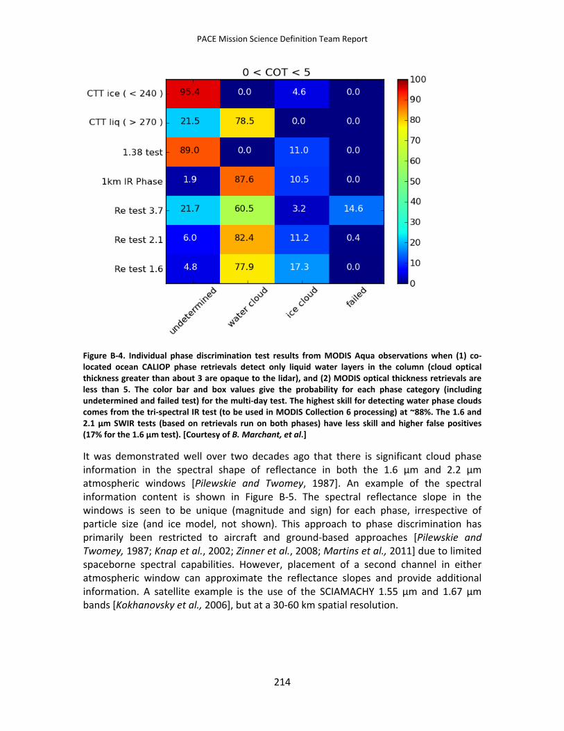
PACE Mission Science Definition Team Report
Figure B-4. Individual phase discrimination test results from MODIS Aqua observations when (1) co-located ocean CALIOP phase retrievals detect only liquid water layers in the column (cloud optical thickness greater than about 3 are opaque to the lidar), and (2) MODIS optical thickness retrievals are less than 5. The color bar and box values give the probability for each phase category (including undetermined and failed test) for the multi-day test. The highest skill for detecting water phase clouds comes from the tri-spectral IR test (to be used in MODIS Collection 6 processing) at ~88%. The 1.6 and 2.1 µm SWIR tests (based on retrievals run on both phases) have less skill and higher false positives (17% for the 1.6 µm test). [Courtesy of B. Marchant, et al.]
It was demonstrated well over two decades ago that there is significant cloud phase information in the spectral shape of reflectance in both the 1.6 µm and 2.2 µm atmospheric windows [Pilewskie and Twomey, 1987]. An example of the spectral information content is shown in Figure B-5. The spectral reflectance slope in the windows is seen to be unique (magnitude and sign) for each phase, irrespective of particle size (and ice model, not shown). This approach to phase discrimination has primarily been restricted to aircraft and ground-based approaches [Pilewskie and Twomey, 1987; Knap et al., 2002; Zinner et al., 2008; Martins et al., 2011] due to limited spaceborne spectral capabilities. However, placement of a second channel in either atmospheric window can approximate the reflectance slopes and provide additional information. A satellite example is the use of the SCIAMACHY 1.55 µm and 1.67 µm bands [Kokhanovsky et al., 2006], but at a 30-60 km spatial resolution.
214
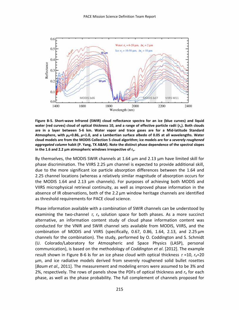
PACE Mission Science Definition Team Report
Figure B-5. Short-wave Infrared (SWIR) cloud reflectance spectra for an ice (blue curves) and liquid water (red curves) cloud of optical thickness 10, and a range of effective particle radii (re). Both clouds are in a layer between 5-6 km. Water vapor and trace gases are for a Mid-latitude Standard Atmosphere, with µ0=0.86, µ=1.0, and a Lambertian surface albedo of 0.05 at all wavelengths. Water cloud models are from the MODIS Collection 5 cloud algorithm; ice models are for a severely roughened aggregated column habit (P. Yang, TX A&M). Note the distinct phase dependence of the spectral slopes in the 1.6 and 2.2 µm atmospheric windows irrespective of re.
By themselves, the MODIS SWIR channels at 1.64 µm and 2.13 µm have limited skill for phase discrimination. The VIIRS 2.25 µm channel is expected to provide additional skill, due to the more significant ice particle absorption differences between the 1.64 and 2.25 channel locations (whereas a relatively similar magnitude of absorption occurs for the MODIS 1.64 and 2.13 µm channels). For purposes of achieving both MODIS and VIIRS microphysical retrieval continuity, as well as improved phase information in the absence of IR observations, both of the 2.2 µm window heritage channels are identified as threshold requirements for PACE cloud science.
Phase information available with a combination of SWIR channels can be understood by examining the two-channel τ, re solution space for both phases. As a more succinct alternative, an information content study of cloud phase information content was conducted for the VNIR and SWIR channel sets available from MODIS, VIIRS, and the combination of MODIS and VIIRS (specifically, 0.67, 0.86, 1.64, 2.13, and 2.25 µm channels for the combination). The study, performed by O. Coddington and S. Schmidt (U. Colorado/Laboratory for Atmospheric and Space Physics (LASP), personal communication), is based on the methodology of Coddington et al. [2012]. The example result shown in Figure B-6 is for an ice phase cloud with optical thickness τ =10, re=20 µm, and ice radiative models derived from severely roughened solid bullet rosettes [Baum et al., 2011]. The measurement and modeling errors were assumed to be 3% and 2%, respectively. The rows of panels show the PDFs of optical thickness and re for each phase, as well as the phase probability. The full complement of channels proposed for
215
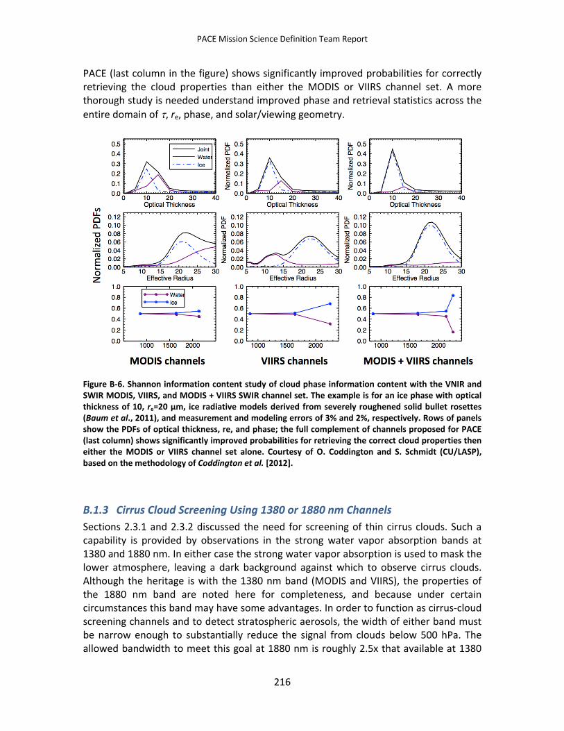
PACE Mission Science Definition Team Report
PACE (last column in the figure) shows significantly improved probabilities for correctly retrieving the cloud properties than either the MODIS or VIIRS channel set. A more thorough study is needed understand improved phase and retrieval statistics across the entire domain of τ, re, phase, and solar/viewing geometry.
Figure B-6. Shannon information content study of cloud phase information content with the VNIR and SWIR MODIS, VIIRS, and MODIS + VIIRS SWIR channel set. The example is for an ice phase with optical thickness of 10, re=20 µm, ice radiative models derived from severely roughened solid bullet rosettes (Baum et al., 2011), and measurement and modeling errors of 3% and 2%, respectively. Rows of panels show the PDFs of optical thickness, re, and phase; the full complement of channels proposed for PACE (last column) shows significantly improved probabilities for retrieving the correct cloud properties then either the MODIS or VIIRS channel set alone. Courtesy of O. Coddington and S. Schmidt (CU/LASP), based on the methodology of Coddington et al. [2012].
B.1.3 Cirrus Cloud Screening Using 1380 or 1880 nm Channels Sections 2.3.1 and 2.3.2 discussed the need for screening of thin cirrus clouds. Such a capability is provided by observations in the strong water vapor absorption bands at 1380 and 1880 nm. In either case the strong water vapor absorption is used to mask the lower atmosphere, leaving a dark background against which to observe cirrus clouds. Although the heritage is with the 1380 nm band (MODIS and VIIRS), the properties of the 1880 nm band are noted here for completeness, and because under certain circumstances this band may have some advantages. In order to function as cirrus-cloud screening channels and to detect stratospheric aerosols, the width of either band must be narrow enough to substantially reduce the signal from clouds below 500 hPa. The allowed bandwidth to meet this goal at 1880 nm is roughly 2.5x that available at 1380
216
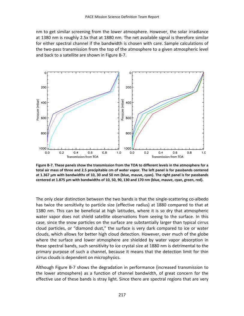
PACE Mission Science Definition Team Report
nm to get similar screening from the lower atmosphere. However, the solar irradiance at 1380 nm is roughly 2.5x that at 1880 nm. The net available signal is therefore similar for either spectral channel if the bandwidth is chosen with care. Sample calculations of the two-pass transmission from the top of the atmosphere to a given atmospheric level and back to a satellite are shown in Figure B-7.
Figure B-7. These panels show the transmission from the TOA to different levels in the atmosphere for a total air mass of three and 2.5 precipitable cm of water vapor. The left panel is for passbands centered at 1.367 µm with bandwidths of 10, 30 and 50 nm (blue, mauve, cyan). The right panel is for passbands centered at 1.875 µm with bandwidths of 10, 50, 90, 130 and 170 nm (blue, mauve, cyan, green, red).
The only clear distinction between the two bands is that the single-scattering co-albedo has twice the sensitivity to particle size (effective radius) at 1880 compared to that at 1380 nm. This can be beneficial at high latitudes, where it is so dry that atmospheric water vapor does not shield satellite observations from seeing to the surface. In this case, since the snow particles on the surface are substantially larger than typical cirrus cloud particles, or “diamond dust,” the surface is very dark compared to ice or water clouds, which allows for better high cloud detection. However, over much of the globe where the surface and lower atmosphere are shielded by water vapor absorption in these spectral bands, such sensitivity to ice crystal size at 1880 nm is detrimental to the primary purpose of such a channel, because it means that the detection limit for thin cirrus clouds is dependent on microphysics.
Although Figure B-7 shows the degradation in performance (increased transmission to the lower atmosphere) as a function of channel bandwidth, of great concern for the effective use of these bands is stray light. Since there are spectral regions that are very
217
PACE Mission Science Definition Team Report
bright over low-level clouds and land surfaces that are close (in wavelength) to the water vapor bands at 1380 and 1880 nm, any out-of-band leaks or scattering of light can render bands of this type useless. Great care must therefore be taken in specifying the out-of-band performance of such channels and testing must be capable of detecting such effects.
B.2 Spatial Resolution There are two purposes to the goal requirement of higher spatial resolution in selected bands as summarized in Table 3-4. The first rationale is the use of high spatial resolution channels to help diagnose the extent to which a non-clear 1 km pixel is appropriate for a cloud retrieval, based on a horizontally homogeneous forward radiative transfer model. In EOS parlance, this is akin to providing Quality Assessment information regarding the cloud retrieval. By default, higher spatial resolution also includes the ability to better distinguish clear from cloudy scenes near cloud boundaries and for broken cloudy scenes. The second rationale is to provide more useful/accurate cloud optical and microphysical retrievals in heterogeneous scenes. Both items are discussed in more detail below.
B.2.1 Cloud Retrieval Quality Assessment (QA): Higher Spatial Resolution VIS/NIR Channels
The MODIS imagers provided separate cloud effective particle radius retrievals derived from three important SWIR and mid-wavelength infrared (MWIR) atmospheric window channels for the first time on the same satellite sensor. For homogeneous clouds, the three effective radius retrievals should be the same (to within basic retrieval uncertainties) and are expected to be reasonably close for adiabatic liquid water clouds [Platnick, 2000]. Therefore, significant differences between the spectral retrievals are indicative of a failure of the forward radiative transfer model. For liquid water clouds in particular, this would include the fact that the cloud radiative model does not account for horizontal photon transport in heterogeneous scenes and/or a vertical microphysical structure, such as the presence of significant dry air entrainment or a drizzle population.
The impact of cloud horizontal heterogeneity on spectral retrievals for boundary-layer water clouds has been discussed by a number of investigators [e.g., Marshak et al., 2006; Hayes et al., 2010; Wolters et al., 2010]. The potential impacts of drizzle on imager spectral size retrievals were investigated in studies by Nakajima et al. [2010a,b], Suzuki et al. [2010], and Sato et al. [2012] using collocated MODIS and CloudSat radar observations. The vertical weighting impact of cloud-top entrainment evaporation has also been discussed in the literature [Seethala and Horváth, 2010]. For ice clouds, a 1D time-dependent model has been used to show that the vertical segregation of particle sizes can contribute to significant spectral size retrieval differences [Zhang et al., 2010].
218
PACE Mission Science Definition Team Report
Distinguishing the effect of horizontal photon transport versus vertical microphysical structure in water clouds is ambiguous, in general, since both can nominally lead to significant positive biases between 1.64 and 2.13 µm size retrievals and a 3.7 µm channel retrieval [e.g., Zhang et al., 2011, 2012].
While there is some deviation in 1.64 and 2.13 µm size retrievals in horizontally heterogeneous scenes, the absence of a 3.7 µm channel on PACE will preclude a straightforward cloud optical retrieval QA assignment, which can be done for MODIS. However, it has been demonstrated that large sub-pixel reflectance heterogeneity in the MODIS 250 m VIS and NIR bands for marine boundary layer water clouds is well-correlated with biases between the spectral MODIS 1 km effective radius retrievals, and can therefore be used to predict the probability of horizontal photon transport biases ([Zhang and Platnick, 2011]; most relevant to upper right quadrant of Figure B-8). Optical thickness view angle biases seen in MISR observations of scenes with small cloud elements, especially subtropical trade cumulus regimes, are also correlated with VIS/NIR 250 m spatial heterogeneity [Liang et al., 2009].
Thus, the goal capability of having 250 m reflectance heterogeneity in the two equivalent MODIS VIS/NIR channels will provide unique information for QA of liquid water cloud optical retrievals over ocean and vegetated land surfaces (see Table 3-4 for channel details).
Higher spatial resolution in the two atmosphere VIS/NIR bands should also provide better QA for aerosol retrievals where it is important to better distinguish cloud-contaminated FOVs in heterogeneous cloud regimes (i.e., trade cumulus and other broken and/or low cloud fraction regimes).
219
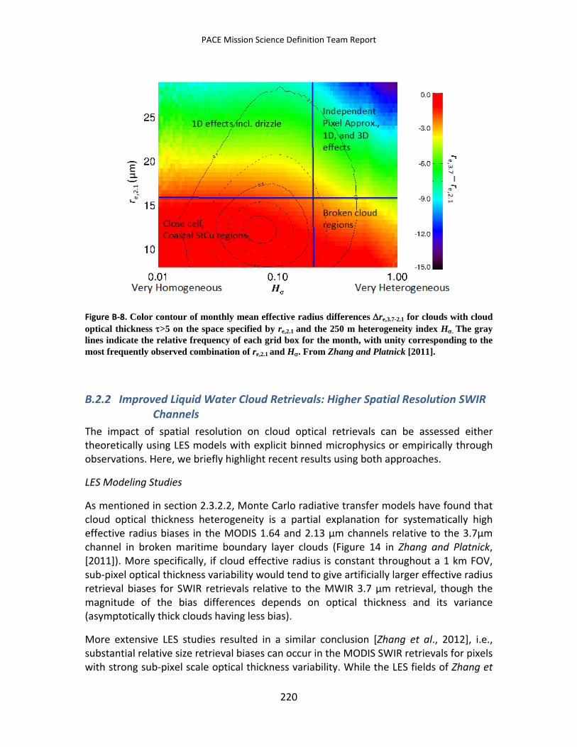
PACE Mission Science Definition Team Report
Figure B-8. Color contour of monthly mean effective radius differences ∆re,3.7-2.1 for clouds with cloud optical thickness τ>5 on the space specified by re,2.1 and the 250 m heterogeneity index Hσ. The gray lines indicate the relative frequency of each grid box for the month, with unity corresponding to the most frequently observed combination of re,2.1 and Hσ. From Zhang and Platnick [2011].
B.2.2 Improved Liquid Water Cloud Retrievals: Higher Spatial Resolution SWIR Channels
The impact of spatial resolution on cloud optical retrievals can be assessed either theoretically using LES models with explicit binned microphysics or empirically through observations. Here, we briefly highlight recent results using both approaches.
LES Modeling Studies
As mentioned in section 2.3.2.2, Monte Carlo radiative transfer models have found that cloud optical thickness heterogeneity is a partial explanation for systematically high effective radius biases in the MODIS 1.64 and 2.13 µm channels relative to the 3.7µm channel in broken maritime boundary layer clouds (Figure 14 in Zhang and Platnick, [2011]). More specifically, if cloud effective radius is constant throughout a 1 km FOV, sub-pixel optical thickness variability would tend to give artificially larger effective radius retrieval biases for SWIR retrievals relative to the MWIR 3.7 µm retrieval, though the magnitude of the bias differences depends on optical thickness and its variance (asymptotically thick clouds having less bias).
More extensive LES studies resulted in a similar conclusion [Zhang et al., 2012], i.e., substantial relative size retrieval biases can occur in the MODIS SWIR retrievals for pixels with strong sub-pixel scale optical thickness variability. While the LES fields of Zhang et
220
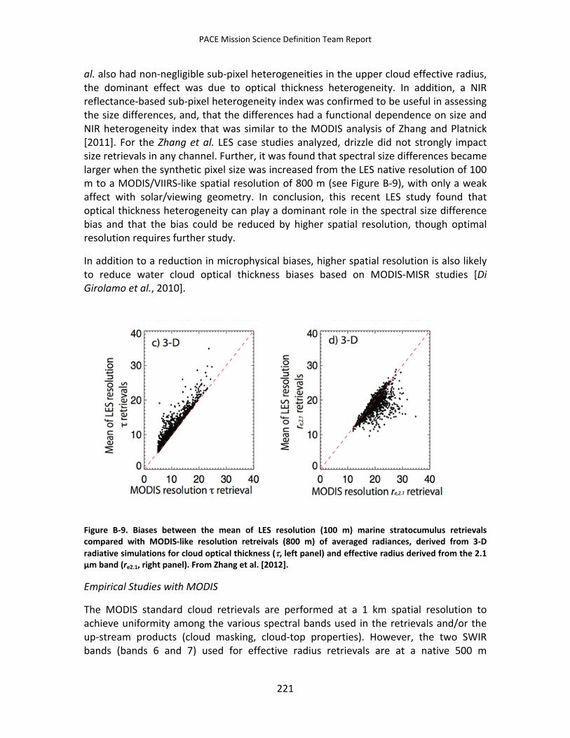
PACE Mission Science Definition Team Report
al. also had non-negligible sub-pixel heterogeneities in the upper cloud effective radius, the dominant effect was due to optical thickness heterogeneity. In addition, a NIR reflectance-based sub-pixel heterogeneity index was confirmed to be useful in assessing the size differences, and, that the differences had a functional dependence on size and NIR heterogeneity index that was similar to the MODIS analysis of Zhang and Platnick [2011]. For the Zhang et al. LES case studies analyzed, drizzle did not strongly impact size retrievals in any channel. Further, it was found that spectral size differences became larger when the synthetic pixel size was increased from the LES native resolution of 100 m to a MODIS/VIIRS-like spatial resolution of 800 m (see Figure B-9), with only a weak affect with solar/viewing geometry. In conclusion, this recent LES study found that optical thickness heterogeneity can play a dominant role in the spectral size difference bias and that the bias could be reduced by higher spatial resolution, though optimal resolution requires further study.
In addition to a reduction in microphysical biases, higher spatial resolution is also likely to reduce water cloud optical thickness biases based on MODIS-MISR studies [Di Girolamo et al., 2010].
Figure B-9. Biases between the mean of LES resolution (100 m) marine stratocumulus retrievals compared with MODIS-like resolution retreivals (800 m) of averaged radiances, derived from 3-D radiative simulations for cloud optical thickness (τ, left panel) and effective radius derived from the 2.1 µm band (re2.1, right panel). From Zhang et al. [2012].
Empirical Studies with MODIS
The MODIS standard cloud retrievals are performed at a 1 km spatial resolution to achieve uniformity among the various spectral bands used in the retrievals and/or the up-stream products (cloud masking, cloud-top properties). However, the two SWIR bands (bands 6 and 7) used for effective radius retrievals are at a native 500 m
221
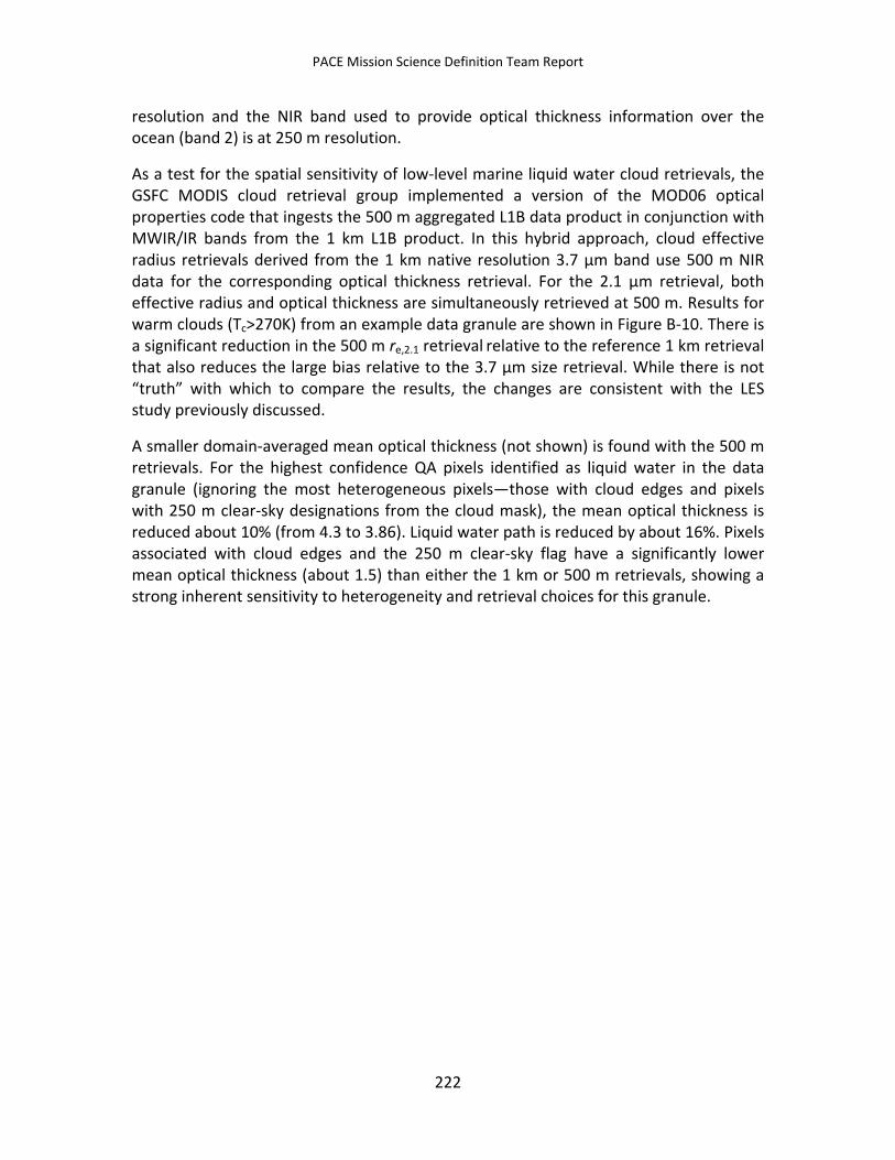
PACE Mission Science Definition Team Report
resolution and the NIR band used to provide optical thickness information over the ocean (band 2) is at 250 m resolution.
As a test for the spatial sensitivity of low-level marine liquid water cloud retrievals, the GSFC MODIS cloud retrieval group implemented a version of the MOD06 optical properties code that ingests the 500 m aggregated L1B data product in conjunction with MWIR/IR bands from the 1 km L1B product. In this hybrid approach, cloud effective radius retrievals derived from the 1 km native resolution 3.7 µm band use 500 m NIR data for the corresponding optical thickness retrieval. For the 2.1 µm retrieval, both effective radius and optical thickness are simultaneously retrieved at 500 m. Results for warm clouds (Tc>270K) from an example data granule are shown in Figure B-10. There is a significant reduction in the 500 m re,2.1 retrieval relative to the reference 1 km retrieval that also reduces the large bias relative to the 3.7 µm size retrieval. While there is not “truth” with which to compare the results, the changes are consistent with the LES study previously discussed.
A smaller domain-averaged mean optical thickness (not shown) is found with the 500 m retrievals. For the highest confidence QA pixels identified as liquid water in the data granule (ignoring the most heterogeneous pixels—those with cloud edges and pixels with 250 m clear-sky designations from the cloud mask), the mean optical thickness is reduced about 10% (from 4.3 to 3.86). Liquid water path is reduced by about 16%. Pixels associated with cloud edges and the 250 m clear-sky flag have a significantly lower mean optical thickness (about 1.5) than either the 1 km or 500 m retrievals, showing a strong inherent sensitivity to heterogeneity and retrieval choices for this granule.
222
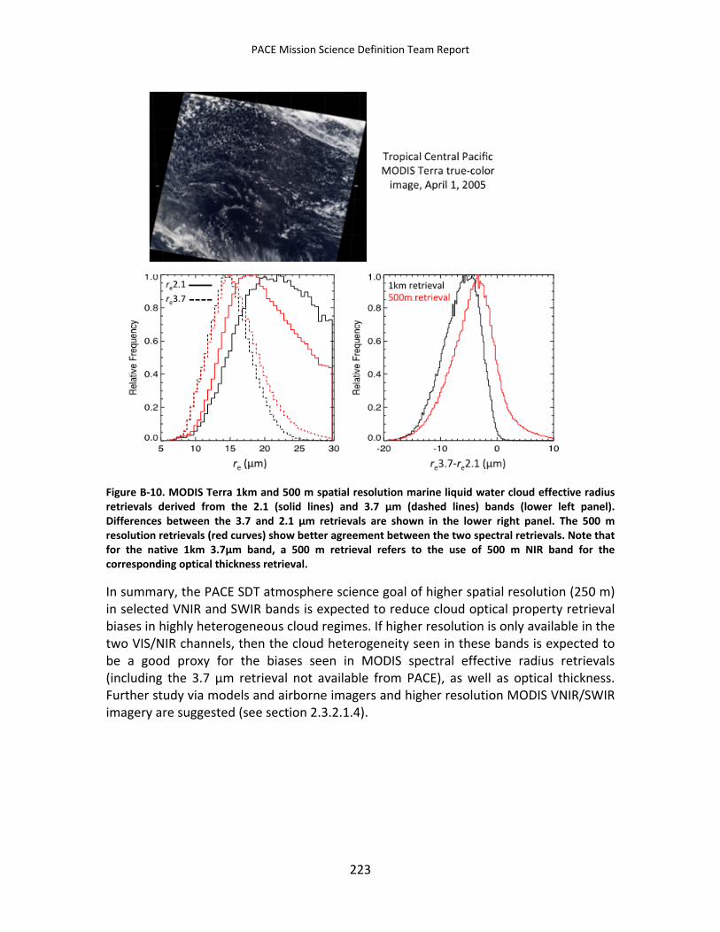
PACE Mission Science Definition Team Report
Figure B-10. MODIS Terra 1km and 500 m spatial resolution marine liquid water cloud effective radius retrievals derived from the 2.1 (solid lines) and 3.7 µm (dashed lines) bands (lower left panel). Differences between the 3.7 and 2.1 µm retrievals are shown in the lower right panel. The 500 m resolution retrievals (red curves) show better agreement between the two spectral retrievals. Note that for the native 1km 3.7µm band, a 500 m retrieval refers to the use of 500 m NIR band for the corresponding optical thickness retrieval.
In summary, the PACE SDT atmosphere science goal of higher spatial resolution (250 m) in selected VNIR and SWIR bands is expected to reduce cloud optical property retrieval biases in highly heterogeneous cloud regimes. If higher resolution is only available in the two VIS/NIR channels, then the cloud heterogeneity seen in these bands is expected to be a good proxy for the biases seen in MODIS spectral effective radius retrievals (including the 3.7 µm retrieval not available from PACE), as well as optical thickness. Further study via models and airborne imagers and higher resolution MODIS VNIR/SWIR imagery are suggested (see section 2.3.2.1.4).
223
PACE Mission Science Definition Team Report
References
References for Section 2.2 Ocean Ecosystems and Biogeochemistry
Ahmad, Z., C. R. McClain, J. R. Herman, B. A. Franz, E. J. Kwaitkowska, W. D. Robinson, E. J. Bucsela, and M. Tzortziou (2007), Atmospheric correction of NO2 in retrieving water-leaving reflectances from the SeaWiFS and MODIS measurements, Appl. Opt., 46(26), 6504-6512.
Ahmad, Z., B. A. Franz, C. R. McClain, E. J. Kwaitkowska, J. Werdell, E. P. Shettle, and B. N. Holben (2010), New aerosol models for the retrieval of aerosol optical thickness and normalized water-leaving radiances from the SeaWiFS and MODIS sensors over coastal regions and open oceans, Appl. Opt., 49(29), 5545-5560.
Alvain, S., C. Moulin, Y. Dandonneau, and F. M. Bréon (2005), Remote sensing of phytoplankton groups in case 1 waters from global SeaWiFS imagery, Deep-Sea Res. I, 52, 1989-2004.
Balch W., D. Drapeau, B. Bowler, and E. Booth (2007), Prediction of pelagic calcification rates using satellite measurements, Deep-Sea Res II, 54, 478-95.
Balch, W. M., B. C. Bowler, D. T. Drapeau, A. Poulton, and P. Holligan (2010), 6960 Biominerals and the vertical flux of particulate organic carbon from the surface 6961 ocean, Geochemical Research Letters, 37(L22605): 1-6, 6962.
Balch, W. M., B. C. Bowler, D. T. Drapeau, A. Poulton, and P. Holligan (2010), Biominerals and the vertical flux of particulate organic carbon from the surface ocean, Geochemical Research Letters, 37, doi:10.1029/2010GL044640.
Balch, W. M., H. R. Gordon, B. C. Bowler, D. T. Drapeau, and E. S. Booth (2005), Calcium carbonate measurements in the surface global ocean based on Moderate-Resolution Imaging Spectrometer data, J. Geophys. Res., 110, C07001, doi:1029/2004JC002560.
Behrenfeld, M. J., K. Worthington, R. M. Sherrell, F. Chavez, P. Strutton, M. McPhaden, and D. Shea (2006), Controls on tropical Pacific ocean productivity revealed through nutrient stress diagnostics, Nature 442, 1025-1028.
Behrenfeld, M. J., T. Westberry, R. O’Malley, J. Wiggert, E. Boss, D. Siegel, B. Franz, C. McClain, G. Feldman, G. Dall’Olmo, A. Milligan, S. Doney, I. Lima, and N. Mahowald (2009), Satellite-detected fluorescence reveals global physiology of ocean phytoplankton, Biogeosciences, 6, 779-794.
224
PACE Mission Science Definition Team Report
Boyd, P. W., and T. W. Trull (2007), Understanding the export of biogenic particles in oceanic waters: Is there consensus?, PROGRESS IN OCEANOGRAPHY, Volume: 72, Issue: 4, 276-312.
Brachter, A., M. Vountas, T. Dinter, J. P. Burrows, R. Rottgers, and I. Peeken (2009), Quantitative observation of cyanobacteria and diatoms from space using PhytoDOAS on SCIAMACHY data, Biogeosciences, 6, 751-764.
Brown, C. W., and J. A. Yoder (1994), Coccolithophorid blooms in the global ocean, J. Geophys, Res. 99: C4, 7467-7482.
Buesseler, K. O. , and P. W. Boyd (2009), Shedding light on processes that control particle export and flux attenuation in the twilight zone, Limnology and Oceanography, 54 (4), 1210–1232.
Chuanmin, H., J. Cannizzaroa, L. Kendall, L. Cardera, F. E. Muller-Kargera, and R. Hardy (2010), Remote detection of Trichodesmium blooms in optically complex coastal waters: Examples with MODIS full-spectral data, Remote Sensing of Environment 114 (9), 2048–2058.
Del Castillo, C. E., and R. L. Miller (2008), On the use of ocean color remote sensing to measure the teransport of dissolved organic carbon by the Mississippi River plume, Remote Sens. Environ., 112, 836-844.
Deutsch, C., J. L. Sarmiento, D. M. Sigman, N. Gruber, and J. P. Dunne (2007), Spatial coupling of nitrogen inputs and losses in the ocean, Nature Vol 445, doi:10.1038/nature05392.
Falkowski, P. G., R. T. Barber, and V. Smetacek (1998), Biogeochemical controls and feedbacks on ocean primary production, Science, 281, 200-206.
Francois, R., S. Honjo, R. Krishfield, and S. Manganini (2002), Factors controlling the flux 6963 of organic carbon to the bathypelagic zone of the ocean, Global Biogeochemical 6964 Cycles, 16(4): doi:10.1029/2001GB001722, 6965.
Francois, R., S. Honjo, R. Krishfield, and S. Manganini (2002), Factors controlling the flux of organic carbon to the bathypelagic zone of the ocean, Global Biogechemical Cycles, 16, 1087.
Gardner, W. D., A. V. Mishonov, and M. J. Richardson (2006), Global POC concentrations from in-situ and satellite data, Deep-Sea Res. II, 53, 718-740.
Gordon, H. R. (1997), Atmospheric correction of ocean color imagery in the Earth 7501 Observing System era, J. Geophys. Res., 102(D14), 17081-17106, 7502.
Gordon, H. R., and M. Wang (1994), Retrieval of water-leaving radiance and aerosol 7503 optical thickness over the oceans with SeaWiFS: A preliminary algorithm, App. 7504 Opt., 33, 443-452.
225
PACE Mission Science Definition Team Report
Gordon, H. R., G. C. Boyton, W. M. Balch, S. B. Groom, D. S. Harbour, and T. J Smyth (2001), Retrieval of coccolithophore calcite concentration from SeaWiFS imagery, Geophys. Res. Lett. 28:8, 1587-1590.
Kostadinov, T. S., D. A. Siegel, and S. Maritorena (2009), Retrieval of the particle size distribution from satellite ocean color observations, J. Geophys. Res., 114, C09015, doi:10.1029/2009JC005303.
La Roche, J., P. W. Boyd, R. M. L. McKay, and R. J. Geider (1996), Flavodoxin as an in situ indicator for iron stress in phytoplankton, Nature, 382, 802-805.
Lee, Z.-P., K. Carder, R. Arnone, and M.-X. He (2007), Determination of primary spectral bands for remote sensing of aquatic environments, Sensors, 7, 3428-3441.
Longhurst, A. (1998), Ecological Geography of the Sea, Academic Press, San Diego, 398.
Mannino, A., M. E. Russ, and S. B. Hooker (2008), Algorithm development and validation for satellite-derived distributions of DOC and CDOM in the U.S. Middle Atlantic Bight, J. Geophys. Res., 113, C07051, doi:10.1029/2007/JC004493.
Martin, J. H., and S. E. Fitzwater (1988), Iron deficiency limits phytoplankton growth in the North-East Pacific subarctic. Nature, 331, 341-343.
Moore, J. K., S. C. Doney, K. Lindsay, N. Mahowald, and A. F. Michaels, (2006), Nitrogen fixation amplifies the ocean biogeochemical response to decadal timescale variations in mineral dust deposition, Tellus, 58B, 560–572.
Moore, J. K., and O. Braucher (2008), Sedimentary and mineral dust sources of dissolved iron to the world ocean, Biogeosciences, 5, 631–656.
Muller-Karger, F. E., R. Varela, R. Thunell, R. Luerssen, C. Hu, and J. J. Walsh (2005), The 6966 importance of continental margins in the global carbon cycle, Geophys. Res. Lett. 6967 32, 1 L01602, 6968.
Muller-Karger, F E., R. Varela, R. Thunell, R. Luerssen, C. Hu, and J. J. Walsh (2005), The importance of continental margins in the global carbon cycle. Geophysical Research Letters, Vol. 32, L01602, doi:10.1029/2004GL021346.
Nelson, N. B., D. A. Siegel, C. A. Carlson, and C. M. Swan (2010), Tracing global biogeochemical cycles and meridional overturning circulation using chromophoric dissolved organic matter, Geophys. Res. Lett., 37, L03610, doi:10.1029/2009GL042325.
Passow, U., and C. L. De La Rocha (2006), Accumulation of mineral ballast on organic 6969 aggregates, Global Biogeochemical Cycles, 20(1).
226
PACE Mission Science Definition Team Report
Passow, U., and C. L. De La Rocha (2006), Accumulation of mineral ballast on organic aggregates, Global Biogeochem, Cycles, 20, GB1013, doi:10.1029/2005GB002579.
Sabine, C. L., R. A. Feely, and N. Gruber( 2004), The oceanic sink for anthropogenic CO(2), Science, Volume: 305, Issue: 5682, 367-371.
Siegel, D. A., S. Maritorena, N. B. Nelson, D. A. Hansell, and M. Lorenzi-Kayser (2002), Global distribution and dynamics of color dissolved and detrital organic materials, J. Geophys. Res., 107:C12, 3228, doi:10.1029/2001JC000965.
Siegel, D. A., S. Maritorena, N. B. Nelson, M. J. Behrenfeld, and C. R. McClain (2005), Colored dissolved organic matter and its influence on the satellite-based characterization of the ocean biosphere, Geophys. Res. Lett., 32, L20605, doi:10.1029/2005GL024310.
Stramski, D., R. A. Reynolds, M. Babin, S. Kaczmarek, M. R. Lewis, R. Röttgers, A. Sciandra, M. Stramska, M. S. Twardowski, B. A. Franz, and H. Claustre (2008), Relationships between the surface concentration of particulate organic carbon and optical properties in the eastern South Pacific and eastern Atlantic Oceans, Biogeosciences, 5, 171-201.
Takahashi, T., S. C. Sutherland, and R. Wanninkhof (2009), Climatological mean and decadal change in surface ocean pCO(2), and net sea-air CO2 flux over the global oceans, DEEP-SEA RESEARCH PART II-TOPICAL STUDIES IN OCEANOGRAPHY Volume 56, Issue: 8-10, 554-577.
Vountas, M., T. Dinter, A. Bracher, J. P. Burrows, and B. Sierk (2007), Spectral Studies of Ocean Water with Space-borne Sensor SCIAMACHY using Differential Optical Absorption Spectroscopy (DOAS), Ocean Sci., 3, 429–440.
Wang, M., and W. Shi (2005), Estimation of ocean contribution at MODIS near-infrared wavelengths along the east coast of the U.S.: Two case studies, Geophys. Res. Lett., 32, L13606, doi:10.1029/2005GL022917.
Westberry, T. K., D. A. Siegel, and A. Subramaniam (2005), An improved bio-optical model for the remote sensing of Trichodesmium spp. Blooms, J. Geophys. Res., 110, C06012, doi 10.1029/2004JC002517.
Westberry, T. K., and D. A. Siegel (2006), Spatial and temporal distribution of Trichodesmium blooms in the world’s oceans, Global Biogeochem, Cycles 20, GB4016, doi:10.1029/2005GB002673.
Wiggert, J. D., R. G. Murtugudde, and J. R. Christian (2006), Annual ecosystem variability in the tropical Indian Ocean: Results of a coupled bio-physical ocean general circulation model, Deep-Sea Res. II, 53, 644-676.
227
PACE Mission Science Definition Team Report
References for Section 2.3 Atmosphere: Aerosols and Clouds
Aerosol/Cloud/Ecosystems (ACE) Mission Science Definition Team documents are available online at http://dsm.gsfc.nasa.gov/ace/library.html.
Bony, S., R. Colman, V.M. Kattsov, R.P. Allan, C.S. Bretherton, J.-L. Dufresne, A. Hall, S. Hallegatte, M.M. Holland, W. Ingram, D.A. Randall, D.J. Soden, G. Tselioudis, and M.J. Webb (2006), How well do we understand and evaluate climate change feedback processes? J. Climate, 19, 3445-3482, doi:10.1175/JCLI3819.1.
Koren, I., L. A. Remer, Y. J. Kaufman, Y. Rudich, and J. V. Martins (2007), On the twilight zone between clouds and aerosols, Geophys. Res. Lett., 34, L08805, doi:10.1029/2007GL029253.
Koren I., G. Feingold, H. L. Jiang, and O. Altaratz (2009), Aerosol effects on the inter-cloud region of a small cumulus cloud field, Geophys. Res. Lett., doi: 10.1029/2009GL037424.
Loeb, N. G., and N. Manalo-Smith (2005), Top-of-atmosphere direct radiative effect of aerosols over global oceans from merged CERES and MODIS observations, J. Climate, 18, 3506-3526.
Persad, G. G., Y. Ming, and V. Ramaswamy (2012), Tropical tropospheric-only responses to absorbing aerosols, J. Climate, 25, 2471–2480, doi: http://dx.doi.org/10.1175/JCLI-D-11-00122.1.
Varnai T., and A. Marshak (2011), Global CALIPSO observations of aerosol changes near clouds Geosci, Remote Sens. Lett. 19-23, 8, Issue 1, 19-23doi:10.1109/LGRS.2010.2049982.
References for Section 2.3.1 Aerosols
Ahmad, Z., B. A. Franz, C. R. McClain, E. J. Kwiatkowska, J. Werdell, E. P. Shettle, and B. N. Holben (2010), New aerosol models for the retrieval of aerosol optical thickness and normalized water-leaving radiances from the SeaWiFS and MODIS sensors over coastal regions and open oceans, Appl Opt 49, 5545-5560.
Bréon, F.-M., and P. Goloub (1998), Cloud droplet effective radius from spaceborne polarization measurements, Geophysical Research Letters, 25, 1879–1882.
228
PACE Mission Science Definition Team Report
Cairns, B., M. Mishchenko, and A. Ackerman et al. (2011), The need for aerosol and cloud measurements from space: Essential contributions from a rapid reflight of the Aerosol Polarimetry Sensor, NASA Goddard Space Flight Center/Goddard Institute for Space Studies, (http://glory.giss.nasa.gov).
CCSP, Chin M., R. Kahn, and S. Schwartz (eds) (2009), (U.S. Climate Change Science Program) synthesis and assessment product 2.3, Atmospheric aerosol properties and climate impacts), 116.
Chowdhary, J., B. Cairns, F. Waquet, K. Knobelspiesse, M. Ottaviani, J. Redemann, L. Travis, and M. Mishchenko (2012), Sensitivity of multiangle, multispectral polarimetric remote sensing over open oceans to water-leaving radiance: Analyses of RSP data acquired during the MILAGRO campaign, Remote Sens. Environ., 118, 284-308, doi:10.1016/j.rse.2011.11.003.
Diner D. J., A. Davis, B. Hancock, S. Geier, B. Rheingans, V. Jovanovic, M. Bull, D. M. Rider, R. A. Chipman, A.-B. Mahler, and S. C. McClain (2010), First results from a dual photoelastic-modulator-based polarimetric camera, Appl Opt 49, 2929-2946.
Dubovik, O., M. Herman, A. Holdak, T. Lapyonok, D. Tanré, J. L. Deuzé, F. Ducos, A. Sinyuk, and A. Lopatin (2011), Statistically optimized inversion algorithm for enhanced retrieval of aerosol properties from spectral multi-angle polarimetric satellite observations, Atmos. Meas. Tech., 4, 975-1018.
Gérard, B., J.-L. Deuzé,, M. Herman, Y. J. Kaufman,, P. Lallart, C. Oudard, et al. (2005), Comparisons between POLDER2 and MODIS/Terra aerosol retrievals over ocean, Journal of Geophysical Research, 110, D24211. doi:10.1029/2005JD006218.
Gordon, H. R., and M. Wang (1994), Retrieval of water-leaving radiance and aerosol optical thickness over oceans with SeaWiFS: a preliminary algorithm, Appl. Opt. 33, 443–452.
Hasekamp, O. P., and J. Landgraf (2005), Retrieval of aerosol properties over the ocean from multispectral single-viewing angle measurements of intensity and polarization: Retrieval approach, information content, and sensitivity study, J. Geophys. Res., 110, D20207, doi:10.1029/2005JD006212.
Hasekamp, O. P., P. Litvinov, and A. Butz (2011), Aerosol properties over the ocean from PARASOL multi-angle photopolarimetric measurements, J. Geophys. Res., 116, D14204, doi:10.1029/2010JD015469.
Herman, M., J.-L. Deuzé, A. Marchant, B. Roger, and P. Lallart (2005), Aerosol remote sensing from POLDER/ADEOS over the ocean: Improved retrieval using a nonspherical particle model, J. Geophys Res., 110, D10S02, doi: 10.1029/2004JD004798.
229
PACE Mission Science Definition Team Report
Hsu, N., S. Tsay, M. King, and J. Herman (2004), Aerosol properties over bright-reflecting source regions, IEEE Trans. Geosci. Remote Sens. 42, 557–569.
IOCCG (International ocean-color coordinating group), Atmospheric Correction for Remotely-Sensed Ocean-Colour Products, Wang, M. (ed.) (2010), Reports of the International Ocean-Colour Coordinating Group, No. 10, IOCCG, Dartmouth, Canada.
IPCC (Inter-governmental Panel on Climate Change), Solomon S., D. Qin, H. Manning, Z. Chen, M. Marquis, K. Averyt, M. Tignor, and H. Miller (eds) (2007), The physical science basis, in Contribution of working group I to the fourth assessment report of the intergovernmental panel on climate change, Cambridge University press.
Jin, Z., and K. Stamnes (1994), Radiative transfer in non-uniformly refracting media such as the atmosphere/ocean system, Applied Optics 33, 431–442.
Kahn, R. A., B. J. Gaitley, M. J. Garay, D. J. Diner, T. Eck, A. Smirnov, and B. N. Holben (2010), Multiangle Imaging SpectroRadiometer global aerosol product assessment by comparison with the Aerosol Robotic Network, J Geophys Res 115:D23209. doi:10.1029/2010JD014601.
Kahn, R. A. (2011), Reducing the uncertainties in direct aerosol radiative forcing. Surveys in Geophysics, doi:10.1007/s10712-011-9153-z.
Kahn, R. A., A. M. Sayer, Z. Ahmad, and B. A. Franz (2012), How aerosol type affects SeaWiFS ocean color retrievals, In preparation.
Knobelspiesse, K., B. Cairns, J. Redemann, R. W. Bergstrom, and A. Stohl (2011), Simultaneous retrieval of aerosol and cloud properties during the MILAGRO field campaign. Atmos. Chem. Phys., doi:10.5194/acp-11-6245-2011.
Knobelspiesse, K., B. Cairns, M. Mishchenko, J. Chowdhary, K. Tsigaridis, B. van Diedenhoven, W. Martin, M. Ottaviani, and M. Alexandrov, (2012), Analysis of fine-mode aerosol retrieval capabilities by different passive remote sensing instrument designs, Optics Express, 20, 21457-21484.
Kokhanovsky, A. A., J. L. Deuzé, D. J. Diner, O. Dubovik, F. Ducos, C. Emde, M. J. Garay, R. G. Grainger, A. Heckel, M. Herman, I. L. Katsev, J. Keller, R. Levy, P. R. J. North, A. S. Prikhach, V. Rozanov, A. M. Sayer, Y. Ota, D. Tanré, G. E. Thomas, and E. P. Zege (2010), The inter-comparison of major satellite aerosol retrieval algorithms using simulated intensity and polarization characteristics of reflected light, Atmos. Meas. Tech., 3, 909–932.
Loeb, N. G. and W. Su (2010), Direct aerosol radiative forcing uncertainty based on a radiative perturbation analysis, J Climate 23:5288–5293.
230
PACE Mission Science Definition Team Report
Levy, R. C., L. A. Remer, R. G. Kleidman, S. Mattoo, C. Ichoku, R. Kahn, and T. F. Eck (2010), Global evaluation of the Collection 5 MODIS dark-target aerosol products over land, Atmos Chem Phys 10:10399–10420. doi:10.5194/acp-10-10399-2010.
McComiskey, A., S. E. Schwartz, B. Schmid, H. Guan, E. R. Lewis, P. Ricchiazzi, and J. A. Ogren (2008), Direct aerosol forcing: calculation from observables and sensitivities to inputs, J Geophys Res 113:D09202. doi:10.1029/2007JD009170.
Mishchenko, M. I., and L. D. Travis (1997a), Satellite retrieval of aerosol properties over the ocean using polarization as well as intensity of reflected sunlight, J Geophys Res 102:16989–17012.
Mishchenko, M. I. and L. D. Travis (1997b), Satellite retrieval of aerosol properties over the ocean using measurements of reflected sunlight: effect of instrumental errors and aerosol absorption, J. Geophys. Res. 102, 13, 543–13, 553.
Mishchenko, M. I., B. Cairns, J. E. Hansen, L. D. Travis, R. Burg, Y. J. Kaufman, J. V. Martins, and E. P. Shettle (2004), Monitoring of aerosol forcing of climate from space: analysis of measurement requirements, J. Quant. Spectrosc. Radiat. Transfer, 88, 149–161.
Mishchenko, M. I., B. Cairns, G. Kopp, C. F. Schueler, B. A. Fafaul, J. E. Hansen, R. J. Hooker, T. Itchkawich, H. B. Maring, and L. D. Travis (2007a), Accurate monitoring of terrestrial aerosols and total solar irradiance: Introducing the Glory mission. Bull. Amer. Meteorol. Soc., 88, 677-691, doi:10.1175/BAMS-88-5-677.
Remer L. A., Y. J. Kaufman, D. Tanre, S. Mattoo, D. A. Chu, J. V. Martins, R.-R Li, C. Ichoku, R. C. Levy, R. G. Kleidman, T. F. Eck, E. Vermote , and B. N. Holben (2005), The MODIS aerosol algorithm, products, and validation, J Atmos Sci 62:947–973.
Remer, L. A., R. G. Kleidman, R. C. Levy, Y. J. Kaufman, D. Tanre, S. Mattoo, J. V. Martins, C. Ichoku, I. Koren, H. Yu, and B. N. Holben (2008), Global aerosol climatology from the MODIS satellite sensors, J Geophys Res 113, doi:10.1029/2007JD009661.
Satheesh, S. K., O. Torres, L. A. Remer, S. S. Babu, V. Vinoj, T. F. Eck, R. G. Kleidman, and B. N. Holben (2009), Improved assessment of aerosol absorption using OMI-MODIS joint retrieval, J. Geophys. Res., 114, D05209, doi:10.1029/2008JD011024.
Tanré, D., F. M. Bréon, J. L. Deuzé, O. Dubovik, F. Ducos, P. François, P. Goloub, M. Herman, A. Lifermann, and F. Waquet (2011), Remote sensing of aerosols by using polarized, directional and spectral measurements within the A-Train: the PARASOL mission, Atmos. Meas. Tech., 4, 1383-1395.
231
PACE Mission Science Definition Team Report
Torres, O., P. K. Bhartia, J. R. Herman, A. Sinyuk, and B. Holben (2002), A long term record of aerosol optical thickness from TOMS observations and comparison to AERONET measurements, J. Atm. Sci. 59:398–413.
Torres, O., A. Tanskanen, B. Veihelman, C. Ahn, R. Braak, P. K. Bhartia, P. Veefkind, and P. Levelt (2007), Aerosols and Surface UV Products from OMI Observations: An Overview, J. Geophys. Res., 112, D24S47, doi:10.1029/2007JD008809.
Torres, O., H. Jethva, and P. K. Bhartia (2011), Retrieval of aerosol optical depth above clouds from OMI obsevations: Sensitivity analysis and cases studies, J. Atmos. Sci., doi:10.1175/JAS-D-11-0130.1, in press.
Wang, M. (2007), Remote sensing of the ocean contributions from ultraviolet to near-infrared using the shortwave infrared bands: simulations, Appl Opt 46,1535-1547.
Waquet, F., B. Cairns, K. Knobelspiesse, J. Chowdhary, L.D. Travis, B. Schmid, and M.I. Mishchenko (2009a), Polarimetric remote sensing of aerosols over land, J. Geophys. Res., 114, D01206, doi:10.1029/2008JD010619.
Waquet, F., J. Riédi, L.-C. Labonnote, P. Goloub, B. Cairns, J.-L. Deuzé, and D. Tanré (2009b), Aerosol remote sensing over clouds using the A-Train observations, J. Atmos. Sci., 66, 2468-2480, doi:10.1175/2009JAS3026.1.
Zhang, J., and J.S. Reid (2010), A decadal regional and global trend analysis of the aerosol optical depth using a data-assimilation grade over-water MODIS and Level 2 MISR aerosol products, Atmos. Chem. Phys, 10, doi:10.5194/acp-10-1-2010.
Zubko V., Y. J. Kaufman, R. I. Burg, and J. V. Martins (2007), Principal Component Analysis of Remote Sensing of Aerosols Over Oceans, IEEE TGRS, No. 3, 45, 730-745.
References for Section 2.3.2 Clouds
Acarreta, J. R., J. F. De Haan, and P. Stamnes (2004), Cloud pressure retrieval using the O2-O2 absorption band at 477 nm, J. Geophys. Res., 109, D05204, doi:10.1029/2003JD003915.
Bréon, F. M., and M. Doutriaux-Boucher (2005), A comparison of cloud droplet radii measured from space, IEEE Trans Geosc. Rem. Sens., Vol. 43, 1796-1805 .doi:10.1109/TGRS.2005.852838.
232
PACE Mission Science Definition Team Report
Coddington, O., P. Pilewskie, S. Schmidt, J. Redemann, S. Platnick, W. Gore, J. Livingston, G. Wind, P. Russell, and T. Vukicevic (2010), Examining the impact of aerosols on the retrieval of cloud optical properties from passive remote sensing, J. Geophys. Res., 115, 13, doi:10.1029/2009JD012829.
Coddington, O., P. Pilewskie, and T. Vukicevic (2012), The Shannon information content of hyperspectral shortwave cloud albedo measurements: Quantification and practical applications, J. Geophys. Res., 117, D04205, doi:10.1029/2011JD016771.
Cole, B. H., P. Yang, B. A. Baum, J. Riedi, L. C. Labonnote, F. Thieuleux and S. Platnick, (2012), Comparison of PARASOL observations with polarized reflectances simulated using different ice habit mixtures, J. Appl. Met. and Climatology, to appear.
Di Girolamo, L., L. Liang, and S. Platnick (2010), A global perspective on the plane-parallel nature of oceanic clouds, Geophy. Res. Letts., 37, 5, doi:10.1029/2010GL044094.
Ferlay, N., F. Thieuleux, C. Cornet, A. B. Davis, P. Dubuisson, F. Ducos, F. Parol, J. Riedi, and C. Vanbauce (2010), Toward new inferences about cloud structures from multidirectional measurements in the oxygen A band: Middle-of-cloud pressure and cloud geometrical thickness from POLDER-3/PARASOL, J. Appl. Meteo. and Climatology, 49, doi:10.1175/2010JAMC2550.1.
Fischer J., and H. Grassl (1991), a: Detection of cloud-top height from backscattered radiances within the oxygen A band. Part 1: Theoretical study. J. Appl. Meteor., 30, 1245–1259.
Fischer J., W. Cordes, A. Schmitz-Pfeifer, W. Renger, and P. Morl (1991), b: Detection of cloud-top height from backscattered radiances within the oxygen A band. Part 2: Measurements, J. Appl. Meteor., 30, 1260–1267.
Fischer, J., R. Preusker, and L. Schüller (1997), ATBD cloud top pressure. European Space Agency Algorithm Theoretical Basis Document, PO-TN-MEL-GS-0006, 28.
Goloub, P., J. L. Deuze, M. Herman, and Y. Fouquart, (1994), Analysis of the POLDER polarization measurements performed over cloud covers, IEEE Transactions on Geoscience and Remote Sensing, 32 (1), 78-88. doi: 10.1109/36.285191.
Haywood, J. M., S. R. Osborne, and S. J. Abel (2004), The effect of overlying absorbing aerosol layers on remote sensing retrievals of cloud effective radius and cloud optical depth, Quarterly J. Royal Meteor. Soc., 130 (598).
Heidinger, A. K., and G. Stephens (2000), Molecular line absorption in a scattering atmosphere. Part II: Application to remote sensing in the O2 A-band. J. Atmos. Sci., 57, 1615-1634.
233
PACE Mission Science Definition Team Report
Holz, R. E., S. A. Ackerman, P. Antonelli, and F. Nagle (2006), An Improvement to the High-Spectral-Resolution CO2-Slicing Cloud-Top Altitude Retrieval. J Atmos. Oceanic Tech., 23, 653-670.
Holz, R. E., S. A. Ackerman, F. W. Nagle, R. Frey, S. Dutcher, R. E. Kuehn, M. A. Vaughan, and B. Baum (2008), Global Moderate Resolution Imaging Spectroradiometer (MODIS) cloud detection and height evaluation using CALIOP. J. Geophys. Res., 113, 1-17.
IPCC: Climate Change 2007: The Physical Science Basis, Contribution of Working Group I to the Fourth Assessment Report of the Intergovernmental Panel on Climate Change, Solomon, S., D. Qin, M. Manning, Z. Chen, M. Marquis, K. B. Averyt, M. Tignor and H. L. Miller (eds.)] (2007), Cambridge University Press, Cambridge, United Kingdom and New York, N.Y., USA.
Johnson, B. T., K. P. Shine, and P. M. Forster, (2004), The semi-direct aerosol effect: Impact of absorbing aerosols on marine stratocumulus, Q. J. R. Meteorol. Soc. (2004), 130, pp 1407–1422 doi: 10.1256/qj.03.61.
Li, S.-W and Q-L Min, (2010), Diagnosis of multilayer clouds using photon path 644 length distributions, J. Geophys. Res. 115, D20202, doi:10.1029/2009JD013774.
Lindstrot, R., R. Preusker, T. Ruhtz, B. Heese, M. Wiegner, C. Lindemann, and J. Fischer (2006), Validation of MERIS cloud-top pressure using airborne lidar measurements, J. Appl. Meteor. Clim., 45, 1612-1621.
Lindstrot R., R. Preusker, and J. Fischer (2010), Remote Sensing of Multilayer Cloud-Top Pressure Using Combined Measurements of MERIS and AATSR on board Envisat. J. Appl. Meteo. and Climatology, 49:6, 1191-1204.
Marshak, A., G. Wen, J. A. Coakley, L. A. Remer, N. G. Loeb, and R. F. Cahalan (2008), A simple model of the cloud adjacency effect and the apparent bluing of aerosols near clouds. J. Geophys. Res., 113, D14S17, doi: 10.1029/2007JD009196.
Martins, J. V., A. Marshak, L. Remer, D. Rosenfeld, Y. J. Kaufman, R. Fernandez-Borda, I. Koren, A. L. Correia, V. Zubko, and P. Artaxo (2011), Remote sensing the vertical profile of cloud droplet effective radius, thermodynamic phase, and temperature, Atmos. Chem. Phys, 11, 9485-9501.
Meyers, K., and S. Platnick (2012), Absorbing smoke over marine boundary layer clouds: CALIOP observations over the southern Atlantic Ocean and effects on MODIS cloud optical property retrievals and radiative forcing, International Radiation Symposium, Berlin.
Minnis, P., P. W. Heck, D. F. Young, C. W. Fairall, and J. B. Snider (1992), Stratocumulus Cloud Properties Derived from Simultaneous Satellite and Island-Based Instrumentation During FIRE, Journal of Applied Meteorology, Vol. 31, 317-339.
234
PACE Mission Science Definition Team Report
Pilewskie, P., and S. Twomey (1987), Discrimination of ice from water in clouds by optical remote sensing, Atmos. Res., 21, 113-122.
Preusker R., and R. Lindstrot (2009), Remote Sensing of Cloud-Top Pressure Using Moderately Resolved Measurements within the Oxygen A Band—A Sensitivity Study, Journal of Applied Meteorology and Climatology, 48:8, 1562-1574.
Randall, D. A., R. A. Wood, S. Bony, R. Colman, T. Fichefet, J. Fyfe, V. Kattsov, A. Pitman, J. Shukla, J. Srinivasan, R. J. Stouffer, A. Sumi, and K. E. Taylor (2007), Climate Models and Their Evaluation., inClimate Change 2007: The Physical Science Basis, Contribution of Working Group I to the Fourth Assessment Report of the Intergovernmental Panel on Climate Change,Solomon, S., D. Qin, M. Manning, Z. Chen, M. Marquis, K. B. Averyt, M. Tignor, and H. L. Miller (eds.), Cambridge University Press, Cambridge, United Kingdom and New York, N.Y., USA.
Riedi, J., B. Marchant, S. Platnick, B. A. Baum, F. Thieuleux, C. Oudard, F. Parol, J. M. Nicolas, and P. Dubuisson (2010), Cloud thermodynamic phase inferred from merged POLDER and MODIS data, Atmos. Chem. Phys., 10, 11851-11865, doi:10.5194/acp-10-11851-2010.
Riedi, J., P. Goloub, R. T. Marchand (2001), Comparison of POLDER cloud phase retrievals to active remote sensors measurements at the ARM SGP site, Geophys. Res. Lett., 28-11, 2185-2188.
Sneep, M., J. de Haan, P. Stammes, P. Wang, C. Vanbauce, J. Joiner, A. P. Vasilkov, and P. F. Levelt (2008), Three way comparison between OMI/Aura and POLDER/PARASOL cloud pressure products, J. Geophys. Res., 113, D15S23, doi:10.1029/2007JD008694, 6188, 6190, 6198, 6203.
Stubenrauch, C. J.,S. Kinne, W. Rossow, et al. (2012), Assessment of Global Cloud Datasets from Satellites, A Project of the World Climate Research Programme Global Energy and Water Cycle Experiment (GEWEX) Radiation Panel.
Stubenrauch, C., S. Kine, W. B. Rossow et al. (2011), GEWEX Cloud Assessment: Scope and status of cloud property products, Workshop on Evaluation of Satellite-Related Global Climate Datasets, WCRP Observations and Assimilation Panel (WOAP), Frascati Italy, (http://climserv.ipsl.polytechnique.fr/gewexca).
Stubenrauch, C. J., and S. Kinne (2009), Assessment of global cloud climatologies, GEWEX News, No. 1, International Project Office, Silver Spring, MD.
Torres, O., H. Jethva, and P. K. Bharatia (2012), Retrieval of aerosol optical depth over clouds from OMI observations: Sensitivity analysis and case studies, J. Atmos. Sci., in press.
235
PACE Mission Science Definition Team Report
Varnai, T., and A. Marshak (2009), MODIS observations of enhanced clear sky reflectance near clouds, Geoph. Res. Lett., 36, L06807, doi:10.1029/2008GL037089.
Wilcox, E. M. (2012) Direct and semi-direct radiative forcing of smoke aerosols over clouds, Atmos. Chem. Phys., 12, 139–149, www.atmos-chem-phys.net/12/139/2012/doi:10.5194/acp-12-139-2012.
Wind, G., S. Platnick, M. D. King, P. A. Hubanks, M. J. Pavolonis, A. K. Heidinger, P. Yang, and B. A. Baum (2010), Multilayer Cloud Detection with the MODIS Near-Infrared Water Vapor Absorption Band, J Appl Met Clim, 49 (11), 2315-2333.
Wu, D., Y. Hu, M. P. McCormick, K. M. Xu, Z. Liu, B. Smith, A. H. Omar, and F. L. Chang, (2008), Deriving Marine-Boundary-Layer Lapse Rate from Collocated CALIPSO, MODIS, and AMSR-E Data to Study Global Low-Cloud Height Statistics, Geoscience and Remote Sensing Letters, IEEE , vol.5, no.4, 649-652.
Zeng, S., C. Cornet, F. Parol, J. Riedi, and F. Thieuleux (2012), A better understanding of cloud optical thickness derived from the passive sensors MODIS/AQUA and POLDER/PARASOL in the A-train constellation, Atmos. Chem. Phys. Discuss., 12, 11733-11764, doi:10.5194/acpd-12-11733-2012.
Zhang, Z., S. Platnick, P. Yang, A. Heidinger, and J. M. Comstock (2010), Effect of ice particle size vertical inhomogeneity on the passive remote sensing of ice clouds, J. Geophys. Res., 115, 16, doi:10.1029/2010JD013835.
Zhang, Z., and S. Platnick (2011), An assessment of differences between cloud effective particle radius for marine water clouds from three MODIS spectral bands. J. Geophys. Res., 116, D20215, doi:10.1029/2011JD016216.
Zinner, T., A. Marshak, S. Lang, J. V. Martins, and B. Mayer (2008), Remote sensing of cloud sides of deep convection: towards a three-dimensional retrieval of cloud particle size profiles, Atmos. Chem. Phys., 8, 4741–4757.
References for Section 2.4 Terrestrial Ecology
Barker, D. H., G. G. R. Seaton, and S. A. Robinson (1997), Internal and external photoprotection in developing leaves of the CAM plant Cotyledon orbiculata, Plant, Cell and Environment 20, 617–624.
Bartley, G. E., and P. A. Scolnik (1995), Plant carotenoids: pigments for photoprotection, visual attraction, and human health, The Plant Cell 7: 1027–1038.
236
PACE Mission Science Definition Team Report
Blackburn, G. A. (2007), Hyperspectral remote sensing of plant pigments, Journal of Experimental Botany 58(4), 855-867.
Broge, N., and E. Leblanc (2002), Deriving green crop area index and canopy chlorophyll density of winter wheat from spectral reflectance data, Remote Sensing of Environment, 81, 45– 57.
Chalker-Scott, L. (1999), Environmental significance of anthocyanins in plant stress responses, Photochemistry and Photobiology 70, 1–9.
Close, D. C., and C. L. Beadle (2003),The ecophysiology of foliar anthocyanin, The Botanical Review 69, 149–161.
Coops, N. C., T. Hilker, F. G. Hall, C. J. Nichol, and G. G. Drolet (2010), Estimation of light-use efficiency of terrestrial ecosystems from space: a status report, Bioscience 60(10), 788-797.
Drolet, G. G., K. F. Huemmrich, F. G. Hall, E. M. Middleton, T. A. Black, A. G. Barr, and H. A. Margolis (2005), A MODIS-derived photochemical reflectance index to detect inter-annual variations in the photosynthetic light-use efficiency of a boreal deciduous forest, Remote Sensing of Environment 98(2-3), 212-224.
Drolet, G. G., E. M. Middleton, K. F. Huemmrich, F. G. Hall, B. D. Amiro, A. G. Barr, T. A. Black, J. H. McCaughey, and H. A. Margolis (2008), Regional mapping of gross light-use efficiency using MODIS spectral indices, Remote Sensing of Environment, 12, 3064-3078.
Fang, Z., J. Bouwkamp, and T. Solomos (1998), Chlorophyllase activities and chlorophyll degradation during leaf senescence in non- yellowing mutant and wild type of Phaseolus vulgaris L, Journal of Experimental Botany 49, 503–510.
Filella I., A. Porcar-Castell, S. Munné-Bosch, J. Bäck, M. F. Garbulsky, and J. Peñuelas (2009), PRI assesment of long-term changes in carotenoids/chlorophyll ratio and short-term changes in de-epoxidation state of the xanthophyll cycle, International Journal of Remote Sensing 30, 4443-4455.
Filella, I., L. Serrano, J. Serra, and J. Peñuelas (1995), Evaluating wheat nitrogen status with canopy reflectance indices and discriminant analysis, Crop Science 35, 1400–1405.
Gamon J. A., and H-L Qiu (1999), Ecological applications of remote sensing at multiple scales, in Pugnaire, F. I., Valladares, F. (Eds.) Handbook of Functional Plant Ecology, 805-846, Marcel Dekker, Inc., New York.
Gamon, J. A., J. Penuelas, and C. B. Field (1992), A narrow-wavelength spectral index that tracks diurnal changes in photosynthetic efficiency, Remote Sens. Environ., 41: 35-44.
237
PACE Mission Science Definition Team Report
Garbulsky M. F., J. Peñuelas, J. Gamon, Y. Inoue, and I. Filella (2011), The photochemical reflectance index (PRI) and the remote sensing of leaf, canopy and ecosystem radiation use efficiencies, A review and meta-analysis, Remote Sensing of Environment 115: 281-297.
Garbulsky M. F., J. Peñuelas, D. Papale, and I. Filella (2008), Remote estimation of carbon dioxide uptake by a Mediterranean forest, Global Change Biology, 14: 2860-2867.
Gitelson, A. (2011), Nondestructive estimation of foliar pigment (Chlorophylls, carotenoids, and anthocyanins) contents: evaluating a semianalytical three band model in Hyperspectral Remote Sensing of Vegetation, edited by P. S. Thenkabail, J. G. Lyon, and A. Huete, CRC Press, ISBN-10: 1439845379.
Goerner, A., M. Reichstein, E. Tomelleri, N. Hanan, S. Rambal, D. Papale, D. Dragoni, and C. Schmullius (2010), Remote sensing of ecosystem light use efficiency with MODIS-based PRI. Biogeosciences, 8, 189-202.
Gould, K. S., J. McKelvie, and K. R. Markham, (2002), Do anthocyanins function as antioxidants in leaves? Imaging of H2O2 in red and green leaves after mechanical injury, Plant, Cell and Environment 25, 1261–1269.
Grace, J., C. Nichol, M. Disney, P. Lewis, T. Quaife, and P. Bowyer (2007), Can we measure terrestrial photosynthesis from space directly, using spectral reflectance and fluorescence? Global Change Biology 13: 1484–1497, doi: 10.1111/j.1365-2486.2007.01352.x.
Haboudane, D., J. Miller, E. Pattey, P. Zarco-Tejada, and I. Strachan (2004), Hyperspectral vegetation indices and novel algorithms for predicting green LAI of crop canopies: Modeling and validation in the context of precision agriculture, Remote Sensing of Environment, 90, 337–352.
Hall, F. G., K. F Huemmrich, and S. N. Goward (1990), Use of narrow band spectra to estimate fraction of absorbed photosynthetically active radiation, Remote Sens. Environ, 32, 47-54.
Hilker, T., N. C. Coops, F. G. Hall, T. A. Black, B. Chen, P. Krishnan, M. A. Wulder, P. J. Sellers, E. M. Middleton, and K. F. Huemmrich (2008), A Modeling Approach for Up-scaling Gross ecosystem production to the landscape scale using remote sensing data, Journal of Geophysical Research – Biogeosciences, 113 (G3): Art. No. G03006.
Hilker, T., A. Gitelson, N. C. Coops, F. G. Hall, and T. A. Black, (2011), Tracking plant physiological properties from multi-angular tower-based remote sensing, Oecologia 165: 865-876.
238
PACE Mission Science Definition Team Report
Huemmrich, K.F. (2001), The GeoSail model: a simple addition to the SAIL model to describe discontinuous canopy reflectance, Remote Sens. Environ. 75, 423-431.
Huemmrich, K. F. and Goward, S. N. (1997), Vegetation canopy PAR absorptance and NDVI: an assessment for ten tree species with the SAIL model, Remote Sens. Environ. 61 (2), 254-269.
Huemmrich, K. F., E. M. Middleton, D. Landis, T. A. Black, A. Barr, J. H. McCaughey, and F. G. Hall (2009), Remote sensing of light use efficiency, Proceedings of the 30th Canadian Symposium on Remote Sensing, June 22-25, 2009, Lethbridge Alberta Canada.
Jung, M. et al. (2007), Uncertainties of modeling gross primary productivity over Europe: A systematic study on the effects of using different drivers and terrestrial biosphere models, Global Biogeochem. Cycles, 21, GB4021, doi:10.1029/2006GB002915.
Lin, J. C., M. R. Pejam, E. Chan, S. C. Wofsy, E. W. Gottlieb, H. A. Margolis, and J. H. McCaughey (2011), Attributing uncertainties in simulated biospheric carbon fluxes to different error sources, Global Biogeochemical Cycles 25, GB2018, doi:10.1029/2010GB003884.
Martel, M. C., H. A. Margolis, C. Coursolle, F. J. Bigras, F. A. Heinsch., and S. W. Running (2005), Decreasing photosynthesis at different spatial scales during the late growing season on a boreal cutover, Tree Physiology 25 (6): 689-699.
Middleton, E. M., K. F. Huemmrich, Y-B. Cheng, and H. A. Margolis (2011), Spectral bio-Indicators of photosynthetic efficiency and vegetation stress in Hyperspectral Remote Sensing of Vegetation, P. S. Thenkabail, J. G. Lyon, and A. Huete, Eds. CRC Press, ISBN-10: 1439845379.
Moran, J. A., A. K. Mitchell, G. Goodmanson, and K. A. Stockburger (2000), Differentiation among effects of nitrogen fertilization treatments on conifer seedlings by foliar reflectance: a comparison of methods, Tree Physiology 20: 1113–1120.
National Aeronautics and Space, Administration, Science Plan for NASA’s Science Mission Directorate 2007–2016, (http://science.nasa.gov/media/medialibrary/2010/03/31/Science_Plan_07.pdf).
National Research Council of the National Academies (2007), Earth Science and Applications from Space: National Imperatives for the Next Decade and Beyond Chapter, The National Academies Press, Washington, D.C.
Nichol, C. J., K. F. Huemmrich, T. A. Black, P. J. Jarvis, C. L. Walthall, J. Grace, and F. G. Hall (2000), Remote sensing of photosynthetic light-use efficiency of boreal forest, Agric. Forest, Meteorol., 101: 131-142.
239
PACE Mission Science Definition Team Report
Peñuelas, J., I. Filella, and J. A. Gamon (1995), Assessment of photosynthetic radiation-use efficiency with spectral reflectance, New Phytol. 131:291-296.
Peñuelas, J., M. F. Garbulsky, and I. Filella (2011), Photochemical reflectance index (PRI) and remote sensing of plant CO2 uptake, New Phytol. 191:596-599.
Raddi, S., F. Magnani, and I. Pippi (2001), Estimation of light use efficiency for the prediction of forest productivity from remote sensing, Proc. 1st SPECTRA Workshop, ESA SP-474,ESTEC, Noordwijk, The Netherlands.
Rahman, A. F., V. D. Cordova, J. A. Gamon, H. P. Schmid, and D. A. Sims (2004), Potential of MODIS ocean bands for estimating CO2 flux from terrestrial vegetation: A novel approach, Geophysical Research Letters 31 (10): Art. No. L10503.
Rahman, A. F., J. A. Gamon, D. A. Fuentes, D. Roberts, and D. Prentiss (2001), Modeling spatially distributed ecosystem flux of boreal forest using hyperspectral indices from AVIRIS imagery, J. Geophy. Res., 106(D24): 33, 579-33, 591.
Richardson, A. D., S. P. Duigan, and G. P. Berlyn (2002), An evaluation of non-invasive methods to estimate foliar chlorophyll content, New Phytologist 153: 185–194.
Steyn, W. J., S. J. E. Wand, D. M. Holcroft, and G. Jacobs (2002), Anthocyanins in vegetative tissues: a proposed unified function in photoprotection, New Phytologist 155, 349–361.
Young, A., and G. Britton (1990), Carotenoids and stress, in Stress Responses in Plants: Adaptation and Acclimation Mechanisms, edited by R. G. Alscher and J. R. Cumming, New York, Wiley-Liss, 87–112.
Zarco-Tejada, P. J., J. R. Miller, A. Morales, A. Berjon, and J. Aguera (2004), Hyperspectral indices and model simulation for chlorophyll estimation in open-canopy tree crops, Remote Sensing of Environment 90, 463–476.
Zarco-Tejada, P. J., J. C. Pushnik, S. Dobrowski, and S. L. Ustin (2003), Steady-state chlorophyll a fluorescence detection from canopy derivative reflectance and double-peak red-edge effects, Remote Sensing of Environment 84, 283–294.
Zhang, Q., E. M. Middleton, H. A. Margolis, G. G. Drolet, A. A. Barr, and T. A. Black (2009), Can a satellite-derived estimate of the fraction of PAR absorbed by chlorophyll (FAPARchl) improve predictions of light-use efficiency and ecosystem photosynthesis for a boreal aspen forest? Remote Sensing of Environment, 113 (4), 880-888.
Zhang, Q., E. M. Middleton, B.-C. Gao, and Y.-B Cheng (2012), Using EO-1 Hyperion to Simulate HyspIRI Products for a Coniferous Forest: the Fraction of PAR Absorbed by Chlorophyll (fAPARchl) and Leaf Water Content (LWC), IEEE Transactions on Geoscience and Remote Sensing, in press.
240
PACE Mission Science Definition Team Report
References for Section 2.5 Watersheds and Lakes
Dall'Olmo, G., and A. A. Gitelson (2006), Effect of bio-optical parameter variability and uncertainties in reflectance measurements on the remote estimation of chlorophyll-a concentration in turbid productive waters: modeling results. Applied Optics 45, 3577-3592.
Darecki, M., and D. Stramski (2004), An evaluation of MODIS and SeaWiFS bio-optical algorithms in the Baltic Sea, Remote Sens. Environ. Lett. 89, 326-350.
Downing, J. A., Y. T. Prairie, J. J. Cole, C. M. Duarte, L. J. Tranvick, R. G. Striegel, W. H. McDowell, P. Kortelainen, J. M. Melack, and J. J. Middleburg (2006), The global abundance and size distribution of lakes, ponds and impoundments, Limnology and Oceanography 51, 2388-2397.
Gitelson, A. A., J. F. Schalles, and C. M. Hladik (2007), Remote chlorophyll-a retrieval in turbid, productive estuaries: Chesapeake Bay case study, Remote Sens. Environ. 109, 464-472.
Gordon, H. R. and A. Y. Morel (1983), Remote assessment of ocean color for interpretation of satellite visible imagery- a review, Springer-Verlag, New York.
Groombridge, B. and M. Jenkins (1998), Freshwater Biodiversity: A Preliminary Global Assessment, World Conservation Monitoring Centre (UNEP-WCMC), World Conservation Press, Cambridge, UK, p. 104p with various maps.
Lucke, R. L., M. Corson, N. R. McGlothlin, S. D. Butcher, D. L. Wood, D. R. Korwan, R. R. Li, W. A. Snyder, C. O. Davis, and D. T. Chen (2011), The Hyperspectral Imager for the Coastal Ocean: instrument description and first images, Applied Optics 50, 1501-1516.
Meybeck, M. (1995), Global distribution of lakes, Springer-Verlag, New York.
NASA (2010), Responding to the Challenge of Climate and Environmental Change: NASA’s Plan for a Climate-Centric Architecture for Earth Observations and Applications from Space, National Aeronautics and Space Administration, Washington, D.C., 48.
Pozdnyakov, D., R. Shuchman, A. Korosov, and C. Hatt (2005), Operational algorithm for the retrieval of water quality in the Great Lakes, Remote Sensing of Environment 97, 352-370.
241
PACE Mission Science Definition Team Report
Schuiling, R. D. (1977), Source and composition of lake sediments in Proceedings of an international symposium on the interaction between sediments and fresh water, edited by H. L. Golterman, Amsterdam, the Netherlands, 12–18.
Stumpf, R. P. (1987), Application of AVHRR satellite data to the study of sediment and chlorophyll in turbid coastal water, NOAA Technical Memorandum NESDIS AISC 7, 1-50.
Stumpf, R. P., R. A. Arnone, R. W. Gould, Jr., P. M. Martinolich, and V. Ransibrahmanakul (2003), A partially coupled ocean-atmosphere model for retrieval of water-leaving radiance from SeaWiFS in coastal waters, Algorithm Updates for the Fourth SeaWiFS Data Reprocessing, SeaWiFS Postlaunch Technical Report Series, NASA, Greenbelt, MD.
Stumpf, R. P., and J. R. Pennock (1989), Calibration of a General Optical Equation for Remote Sensing of Suspended Sediments in a Moderately Turbid Estuary, Journal of Geophysical Research 94 (C10), 14, 363-314, 371.
Wetzel, R. W. (1990), Land-water interfaces: Metabolic and limnological regulators [In German], Int. Verein. Theor. Limnol. Verh. 24, 6-24.
Witter, D. L., J. D. Ortiz, S. Palm, R. T. Heath, and J. W. Budd (2009), Assessing the application of SeaWiFS ocean color algorithms to Lake Erie, Journal of Great Lakes Research 35, 361-370.
References for Section 3.2 Ocean Ecology and Biogeochemistry
Ahmad, Z., B. A. Franz, C. R. McClain, E. J. Kwiatkowska, J. Werdell, E. P. Shettle, and B. N. Holben (2010), New aerosol models for the retrieval of aerosol optical thickness and normalized water-leaving radiances from the SeaWiFS and MODIS sensors over coastal regions and open oceans, Appl Opt 49, 5545-5560.
Antoine, D., A. Morel, H. R. Gordon, V. F. Banzon, and R. H. Evans (2005), Bridging ocean color observations of the 1980s and 2000s in search of long-term trends, J. Geophys. Res., 110, C06009, doi:10.1029/2004JC002620.
Barnes, R. A., A. W. Holmes, and W.E. Esaias (1995), Stray Light in the SeaWiFS Radiometer,NASA Tech. Memo. 104566, Vol. 31, S.B. Hooker, E.R. Firestone, and J.G. Acker, Eds., NASA Goddard Space Flight Center, Greenbelt, Maryland.
Chowdhary, J., B. Cairns, F. Waquet, K. Knobelspiesse, M. Ottaviani, J. Redemann, L. Travis, and M. Mishchenko (2012), Sensitivity of multiangle, multispectral polarimetric remote sensing over open oceans to water-leaving radiance:
242
PACE Mission Science Definition Team Report
Analyses of RSP data acquired during the MILAGRO campaign, Remote Sens. Environ., 118, 284-308, doi:10.1016/j.rse.2011.11.003.
Dubovik, O., B. Holben, T. Eck, A. Smirnov, Y. Kaufman, M. King, D. Tanré, and I. Slutsker (2002), Variability of absorption and optical properties of key aerosol types observed in worldwide locations, J. Atmos. Sci., 59(3), 590–608.
Dubuisson, P., R. Frouin, D. Dessailly, L. Duforêt, J.-F., Léon, K. Voss, and D. Antoine (2009), Estimating the altitude of aerosol plumes over the ocean from reflectance ratio measurements in the O2 A-band, Remote Sensing of Environment 113, 1899–1911.
Duforêt, L., R. Frouin, and P. Dubuisson (2007), Importance and estimation of aerosol vertical structure in satellite ocean-colour remote sensing, Applied Optics, 46, 1107−1119.
Franz, B. A., P. J. Werdell, G. Meister, E. J. Kwiatkowska, S. W. Bailey, Z. Ahmad, and C. R. McClain (2006), MODIS land bands for ocean remote sensing applications, Proc. Ocean Optics, Montreal, 12.
Gordon, H. R. (1990), Radiometric considerations for ocean color remote sensors, App. Opt., 29, 3228-3236.
Gordon, H. R. (1997), Atmospheric correction of ocean color imagery in the Earth Observing System era, J. Geophys. Res., 102(D14), 17081-17106.
Gordon, H. R., and M. Wang (1994), Retrieval of water-leaving radiance and aerosol optical thickness over the oceans with SeaWiFS: A preliminary algorithm, App. Opt., 33, 443-452, DRAFT237.
Gordon, H. R., T. Du, and T. Zhang (1997), Atmospheric correction of ocean color sensors: analysis of the effects of residual instrument polarization sensitivity, Appl. Opt., 36(27), 6938-6948.
Gregg, W.W., and F.S. Patt (1994), Assessment of tilt capability for spaceborne global ocean color sensors, IEEE Trans. Geosci. & Remote Sens., 33(4), 866-877.
IOCCG (2010), Atmospheric Correction for Remotely-Sensed Ocean-Color Products in Reports of International Ocean-Color Coordinating Group No. 10, M. Wang, Ed., IOCCG, Dartmouth, Canada.
Jin, Z., and K. Stamnes (1994), Radiative transfer in nonuniformly refracting layered media: atmosphere-ocean system, Appl. Opt., Vol. 33, Issue 3, 431-442.
Jin, Z., and K. Stamnes (1994), Radiative transfer in non-uniformly refracting media such as the atmosphere/ocean system, Applied Optics 33, 431–442.
243
PACE Mission Science Definition Team Report
Kahn, R. A., A. M. Sayer, Z. Ahmad, and B. A. Franz (2012), How aerosol type affects SeaWiFS ocean color retrievals, in preparation.
McClain, C., A Decade of Satellite Ocean Color Observations. ANNU REV MAR SCI. 2009; 1 19-42.
Maritorena S., O. Hembise F. d’Andon, A. Mangin, and D. A. Siegel (2010), Merged Satellite Ocean Color Data Products Using a Bio-Optical Model: Characteristics, Benefits and Issues, Remote Sensing of Environment, 114, 8, 1791-1804.
Martinez, E., D. Antoine, F. D'Ortenzio, and B. Gentili (2009), Climate-driven basin-scale decadal oscillations of oceanic phytoplankton, Science, 326, 1253-1256.
Meister, G. and C. R. McClain (2010), Point-spread function of the ocean color bands of the Moderate Resolution Imaging Spectroradiometer on Aqua, Applied Optics, 49(32), 6276–6285.
Meister, G., C. McClain, Z. Ahmad, S. Bailey, R. Barnes, S. Brown, G. Eplee, B. Franz, A. Holmes, B. Monosmith, F. Patt, R. Stumpf, K. Turpie, and J. Werdell (2011), Requirements for an Advanced Ocean Radiometer, NASA T/M-2011-215883, NASA Goddard Space Flight Center, Greenbelt, Maryland, 40.
Mishchenko, M., B. Cairns, G. Kopp, C. Schueler, B. Fafaul, J. Hansen, R. Hooker, T. Itchkawich, H. Maring, and L. Travis (2007), Accurate monitoring of terrestrial aerosols and total solar irradiance: introducing the Glory mission, Bull. Amer. Meteorol. Soc, 88, 687–691.
Patt, F. S., R. A. Barnes, R. E. Eplee, Jr., B. A. Franz, W. D. Robinson, G. C. Feldman, S. W. Bailey, J. Gales, P. J. Werdell, M. Wang, R. Frouin, R. P. Stumpf, R. A. Arnone, R. W. Gould, Jr., P. M. Martinolich, V. Ransibrahmanakul, J. E. O'Reilly, and J. A. Yoder (2003), Algorithm Updates for the Fourth SeaWiFS Data Reprocessing, NASA Tech. Memo. 2003--206892, Vol. 22, S. B. Hooker and E. R. Firestone, Eds., NASA Goddard Space Flight Center, Greenbelt, Maryland.
Shi, W., and M. Wang (2007), Detection of turbid waters and absorbing aerosols for the MODIS ocean color data processing, Remote Sens. Environ., 110, 149-161.
Siegel, D. A., and B.A. Franz (2010), Century of phytoplankton change, Nature, 466, 569-571, doi:10.1038/466569.a.
Wang, M. (2007), Remote sensing of the ocean contributions from ultraviolet to near- infrared using the shortwave infrared bands: simulations, Appl Opt 46, 1535-7133.
Wang, M. and H. Gordon (2002), Calibration of ocean color scanners: how much error is acceptable in the near infrared?, Remote Sensing of Environment, Vol. 82, 497-504.
244
PACE Mission Science Definition Team Report
Yeh, E-n., R.A. Barnes, M. Darzi, L. Kumar, E.A. Early, B.C. Johnson, J.L.Mueller, and C.C. Trees (1997), Case Studies for SeaWiFS Calibration and Validation, Part 4, NASA Tech. Memo 104566, Vol. 41, S.B. Hooker and E.R. Firestone, Eds., NASA Goddard Space Flight Center, Greenbelt, Maryland.
References for Section 3.3 PACE Atmosphere Measurement Requirements
Ackerman, S. A. et al. (2008), Cloud Detection with MODIS: Part II Validation. J. Atmos. Oceanic Technol., 25, 1073-1086.
Lindstrot R., R. Preusker, and J. Fischer (2010), Remote Sensing of Multilayer Cloud-Top Pressure Using Combined Measurements of MERIS and AATSR on board Envisat. J. Appl. Meteo. and Climatology, 49:6, 1191-1204.
Martins, J. V., A. Marshak, L. Remer, D. Rosenfeld, Y. J. Kaufman, R. Fernandez-Borda, I. Koren, A. L. Correia, V. Zubko, and P. Artaxo (2011), Remote sensing the vertical profile of cloud droplet effective radius, thermodynamic phase, and temperature Atmos. Chem. Phys, 11, 9485-9501.
Meyers, K., and S. Platnick (2012), Absorbing smoke over marine boundary layer clouds: CALIOP observations over the southern Atlantic Ocean and effects on MODIS cloud optical property retrievals and radiative forcing, International Radiation Symposium, Berlin.
Pilewskie, P., and S. Twomey (1987), Discrimination of ice from water in clouds by optical remote sensing, Atmos. Res., 21, 113-122.
Wind, G., S. Platnick, M. D. King, P. A. Hubanks, M. J. Pavolonis, A. K. Heidinger, P. Yang, and B. A. Baum (2010), Multilayer Cloud Detection with the MODIS Near-Infrared Water Vapor Absorption Band, J Appl Met Clim, 49 (11), 2315-2333.
Zinner, T., A. Marshak, S. Lang, J. V. Martins, and B. Mayer (2008), Remote sensing of cloud sides of deep convection: towards a three-dimensional retrieval of cloud particle size profiles, Atmos. Chem. Phys., 8, 4741–4757.
Reference for Section 3.4 Terrestrial Ecology
Townshend, J. R. G., and C. O. Justice (1988), Selecting the spatial resolution of satellite sensors required for global monitoring of land transformations, International Journal of Remote Sensing, 9(2), 187-236.
245
PACE Mission Science Definition Team Report
References for Section 4.4 Onboard Calibration Requirements
Delwart, S., and L. Bourg (2009), Radiometric calibration of MERIS, Proc. SPIE, Vol. 7474, 74740U-1-74740U-12.
Eplee, R. E., F. S. Patt, R. A. Barnes, and C. R. McClain (2007), SeaWiFS long-term solar diffuser reflectance and sensor noise analyses, Applied Optics, Vol. 46, No. 5, 762-773.
Eplee, R. E., J. Sun, G. Meister, F. S. Patt, T. C. Stone, X. Xiong, and C. R. McClain (2011), Cross Calibration of SeaWiFS and MODIS Using On-Orbit Observations of the Moon, Applied Optics, Vol. 50, No. 2, 120-133.
International Ocean-Colour Coordinating Group (IOCCG), Mission Requirements for Future Ocean Colour Sensors, IOCCG Report (submitted), 2012.,
Kieffer, H. H. (1997), Photometric Stability of the Lunar Surface, Icarus, 130, 323-327.
Kieffer, H. H., and T. S. Stone (2005), The spectral irradiance of the Moon, Astronomical Journal, 129, 2887-2901.
Kwiatkowska, E. J., B. A. Franz, G. Meister, C. R. McClain, and X. Xiong (2008), Cross-Calibration of ocean color bands from Moderate Resolution Imaging Spectroradiometer on Terra platform, Applied Optics, vol. 47, no. 36, 6796-6810.
Meister, G., B. A. Franz, E. J. Kwiatkowska, and C. R. McClain (2012), Corrections to the Calibration of MODIS Aqua Ocean Color Bands derived from SeaWiFS Data, IEEE Transactions on Geoscience and Remote Sensing, Vol. 50, No. 1, 310-319.
Stone, T. S., and H. H. Kieffer (2004), Assessment of Uncertainty in ROLO Lunar Irradiance for On-Orbit Calibration, Proc. of SPIE, Vol. 5542, 300-310.
Sun, J., X. Xiong, and W. L. Barnes (2005), MODIS Reflective Solar Diffuser Stability Monitor Sun View Modelling, IEEE Tr. on Geoscience and Remote Sensing, Vol. 43, No. 8, 1845-1854.
Sun, J., X. Xiong, W. L. Barnes, and B. Guenther (2007), MODIS Reflective Solar Bands On-Orbit Lunar Calibration, IEEE Tr. on Geoscience and Remote Sensing, Vol. 45, No. 7, 2383-2393.
Wolfe, R. E., M. Nishihama, A. J. Fleig, J. A. Kuyper, D. P. Roy, J. C. Storey, and F. S. Patt (2002), Achieving sub-pixel geolocation accuracy in support of MODIS land science, Vol. 83, 31-49.
246
PACE Mission Science Definition Team Report
Xiong, X., J. Sun, S. Xiong, and W. L. Barnes (2004), Using the Moon for MODIS On-Orbit Spatial Characterization, Proc. of SPIE, Vol. 5234, 480-487.
Xiong, X., N. Che, and W. L. Barnes (2005), Terra MODIS On-Orbit Spatial Characterization and Performance, IEEE Tr. on Geoscience and Remote Sensing, Vol. 43, No. 2, 355-365.
Xiong, X., N. Che, and W. L. Barnes (2006), Terra MODIS On-Orbit Spectral Characterization and Performance, IEEE Tr. on Geoscience and Remote Sensing, Vol. 44, No. 8, 2198-2206.
References for Section 4.6.1 Field Program Requirements: Oceans
Antoine, D., F. d’Ortenzio, S. B. Hooker, G. Bécu, B. Gentili, D. Tailliez, and A. J. Scott (2008), Assessment of uncertainty in the ocean reflectance determined by three satellite ocean color sensors (MERIS, SeaWiFS, and MODIS-A) at an offshore site in the Mediterranean Sea (BOUSSOLE project), J. Geophys. Res. 113, C07013, doi:10.1029/2007JC004472.
Bailey, S. W., and P. J. Werdell (2006), A multi-sensor approach for the on-orbit validation of ocean color satellite data products, Rem. Sens. Environ. 102, 12-23.
Barnes, R. A., R. E. Eplee, Jr., S. F. Biggar, K. J. Thome, E. F. Zalewski, P. N. Slater, and A. W. Holmes (1999), The SeaWiFS solar radiation-based calibration and the Transfer-to-Orbit Experiment, NASA/TM-1999-206892, Vol. 5, NASA GSFC, Greenbelt, Maryland, 28.
Barnes, R. A., D. K. Clark, W. E. Esaias, G. S. Fargion, G. C. Feldman, and C. R. McClain (2003), Development of a consistent multi-sensor global ocean colour time series, Int. J. Rem. Sens. 24, 4047-4064.
Barnes, W. L., T. S. Pagano, and V. V. Salomonson (1998), Prelaunch characteristics of the Moderate Resolution Imaging Spectroradiometer (MODIS) on EOS-AM1, IEEE Trans. Geo. Rem. Sens. 36, 1088-1100.
Brown, S. W. et al. (2007), The Marine Optical BuoY (MOBY) radiometric calibration and uncertainty budget for ocean color satellite sensor vicarious calibration, Proc. SPIE 6744, doi:10.1117/12.737400.
Clark, D. K., H. R. Gordon, K. J. Voss, Y. Ge, W. Broenkow, and C. Trees (1997), Validation of atmospheric correction over the oceans, J. Geophys. Res. 102, 17209-17217.
247
PACE Mission Science Definition Team Report
Eplee, Jr., R. E., G. Meister, F. S. Patt, B. A. Franz, and C. R. McClain (2011), Uncertainty assessment of the SeaWiFS on-orbit calibration, Proc. SPIE 8153, 81530B, doi:10.1117/12.892340.
Eplee, Jr., R. E., J-Q. Sun, G. Meister, F. S. Patt, X. Xiong, and C. R. McClain (2011), Cross calibration of SeaWiFS and MODIS using on-orbit observations of the Moon, Appl. Opt. 50, 120-133.
Fargion, G. S., and C. R. McClain (2003), SIMBIOS Project 2002 annual report, NASA/TM-2003-211622, NASA GSFC, Greenbelt, Maryland, 157.
Fougnie, B., G. Bracco, B. Lafrance, C. Ruffel, O. Hagolle, and C. Tinel (2007), PARASOL in-flight calibration and performance, Appl. Opt. 46, 5435-5451.
Franz, B. A., S. W. Bailey, P. J. Werdell, and C. R. McClain (2007), Sensor independent approach to the vicarious calibration of satellite ocean color radiometry, Appl. Opt. 45, 5068-5082.
Gordon, H. R. (1998), In-orbit calibration strategy for ocean color sensors, Rem. Sens. Environ. 63, 265-278.
Hooker, S. B., W. E. Esaias, G. C. Feldman, W. W. Gregg, and C. R. McClain (1992), An overview of SeaWiFS and ocean color, NASA/TM-104566, Vol. 1, NASA GSFC, Greenbelt, Maryland, 24.
Hooker, S. B., G. Lazin, G. Zibordi, and S. McLean (2002), An evaluation of above- and in-water methods for determining water-leaving radiances, J. Atmos. Oceanic Tech. 19, 486-515.
Hooker, S. B et al. (2009), The third SeaWiFS HPLC Analysis Round-Robin Experiment (SeaHARRE-3), NASA/TM-2009-215849, NASA GSFC, Greenbelt, Maryland, 97.
Kostadinov, T. S., D. A. Siegel, S. Maritorena, and N. Guillocheau (2007), Ocean color observations and modeling for an optically complex site: Santa Barbara Channel, California, USA, J. Geophys. Res. 112, C07011, doi:10.1029/2006JC003526.
Kwiatkowska, E. J, B. A. Franz, G. Meister, C. R. McClain, and X. Xiong (2008), Cross calibration of ocean-color bands from Moderate Resolution Imaging Spectroradiometer on Terra platform, Appl. Opt. 47, 6796-6810.
Stumpf, R. P. and P. J. Werdell (2010), Adjustment of ocean color sensor calibration through multi-band statistics, Optics Express 18, 401-412.
Werdell, P. J., and S. W. Bailey (2005), An improved in-situ bio-optical data set for ocean color algorithm development and satellite data product validation, Rem. Sens. Environ. 98, 122-140.
248
PACE Mission Science Definition Team Report
Zibordi, G, S. B. Hooker, J. F. Berthon, and D. D’Alimonte (2002), Autonomous above-water radiance measurements from an offshore platform: A field assessment experiment, J. Atmos. Oceanic Tech. 19, 808-819.
References for Section 4.6.2 Field Program Requirements: Aerosols and Section 4.6.3 Field Program Requirements: Clouds
Abdelmonem, A., M. Schnaiter, P. Amsler, E. Hesse, J. Meyer, and T. Leisner (2011), First correlated measurements of the shape and light scattering properties of cloud particles using the new Particle Habit Imaging and Polar Scattering (PHIPS) probe, Atmos. Meas. Tech., 4, 2125-2142, doi:10.5194/amt-4-2125-2011.
Anderson, T. L., and J. A. Ogren (1998), Determining aerosol radiative properties using a TSI 3563 integrating nephelometer, Aerosol Sci. Technol., 29, 57–69, doi:10.1080/02786829808965551.
Anderson, T. L., S. J. Masonis, D. S. Covert, N. C. Ahlquist,, S. G. Howell, A. D. Clarke, and C. S. McNaughton (2003), Variability of aerosol optical properties derived from in situ aircraft measurements during ACE-Asia, J. Geophys. Res., 108(D23), 8647, doi:10.1029/2002jd003247.
Baumgardner, D. et al. (2011), Airborne instruments to measure atmospheric aerosol particles, clouds and radiation: A cook’s tour of mature and emerging technology, Atmos. Res., 102, 10–29, doi:10.1016/j.atmosres.2011.06.021.
Baynard, T., E. R. Lovejoy, A. Pettersson, S. S. Brown, D. Lack, H. Osthoff, P. Massoli, S. Ciciora, W. P. Dube, and A. R. Ravishankara (2007), Design and Application of a Pulsed Cavity Ring-Down Aerosol Extinction Spectrometer for Field Measurements, Aerosol Science and Technology, 41, 4, doi:10.1080/02786820701222801.
Bennartz, R. (2007), Global assessment of marine boundary layer cloud droplet number concentration from satellite, J. Geophys. Res., 112, D02201, doi:10.1029/2006JD007547.
Bond, T. C., T. L. Anderson, and D. Campbell (1999), Calibration and intercomparison of filter-based measurements of visible light absorption by aerosols, Aerosol Sci. Technol., 30(6), 582–600.
Campbell, J. R., J. L. Tackett, J. S. Reid, J. Zhang, D. L. Westphal, M. Vaughan, D. M. Winker, E. J. Welton, J. M. Prospero, A. Shimizu, and N. Sugimoto (2011), Evaluating CALIOP Nighttime Level 2 Aerosol Profile Retrievals Using a Global Transport Model Equipped with Two-Dimensional Variational Data Assimilation
249
PACE Mission Science Definition Team Report
and Ground-Based LiDAR measurements, American Geophysical Union, Fall Meeting 2011, Abstract #A52D-04.
Canadian Broadcasting Corporation (CBC) (2012), Canada’s air pollution experts moved to ‘other priorities,’ <http://www.cbc.ca/news/technology/story/2012/02/15/pol-environmental-monitoring-stations.html>.
Canagaratna, M. R., J. T. Jayne, J. L. Jimenez, J. D. Allan, M. R. Alfarra, Q. Zhang, T. B. Onasch, F. Drewnick, H. Coe, A. Middlebrook, A E. Delia, L. R. Williams, A. Trimborn, M. J. Northway, P. F. DeCarlo, C. E. Kolb, P. Davidovits, and D. R. Worsnop (2007), Chemical and Microphysical Characterization of Ambient Aerosols with the Aerodyne Aerosol Mass Spectrometer, Mass Spectrom. Rev., 26, 185–222, doi:10.1002/mas.20115.
Cappa, C. D., D. A. Lack, J. B. Burkholder, and A. R. Ravishankara (2008), Bias in Filter-Based Aerosol Light Absorption Measurements Due to Organic Aerosol Loading: Evidence from Laboratory Measurements, Aerosol Sci. Technol., 42, 1022–1032, doi:10.1080/02786820802389277.
Chen, S., and E. Firing (2006), Currents in the Aleutian Basin and subarctic North Pacific near the dateline in summer 1993, Journal of Geophysical Research, 111(C03001), doi:10.1029/2005JC003064.
Chiu, J. C., C.-H. Huang, A. Marshak, I. Slutsker, D. M. Giles, B. N. Holben, Y. Knyazikhin, and W. J. Wiscombe (2010), Cloud optical depth retrievals from the Aerosol Robotic Network (AERONET). J. Geophys. Res., 115, D14202, doi:10.1029/2009JD013121.
Chiu, J. C., A. Marshak, Y. Knyazikhin, W. J. Wiscombe, H. W. Barker, J. C. Barnard, and Y. Luo (2006), Remote sensing of cloud properties using ground-based measurements of zenith radiance. J. Geophys. Res., 111, D16201, doi:10.1029/2005JD006843.
Chowdhary, J., B. Cairns, F. Waquet, K. Knobelspiesse, M. Ottaviani, J. Redemann, L. Travis, and M. Mishchenko (2012), Sensitivity of multiangle, multispectral polarimetric remote sensing over open oceans to water-leaving radiance: Analyses of RSP data acquired during the MILAGRO campaign, Remote Sensing of environment, 118, 284-308, doi: 10.1016/j.rse.2011.11.003.
Cotton, R., S. Osborne, Z. Ulanowski, E. Hirst, P. H. Kaye, and R. S. Greenaway (2010), The ability of the small ice detector (SID-2) to characterize cloud particle and aerosol morphologies obtained during flights of the FAAM BAE-146 research aircraft, J. Atmos. Oceanic Technol., 27, 290–303.
DeCarlo, P. F., R. E. Kimmel, A. Trimborn, M. J. Northway, J. T. Jayne, A. C. Aiken, M. Gonin, K. Fuhrer, T. Horvath, K. S. Docherty, D. R. Worsnop, and J. L. Jimenez
250
PACE Mission Science Definition Team Report
(2006), Field-Deployable, High-Resolution, Time-of-Flight Aerosol Mass Spectrometer, Anal. Chem., 78, 8281–8289, doi:10.1021/ac061249n.
Dibb, J. E., R. W. Talbot, E. M. Scheuer, G. Seid, M. A. Avery, and H. B. Singh (2003), Aerosol chemical composition in Asian continental outflow during the TRACE-P campaign: Comparison with PEM-West B, J. Geophys. Res., 108(D21), GTE 36-1–GTE 36-13b.
Diner, D. J., T. P. Ackerman, A. J. Braverman, C. J. Bruegge, M. J. Chopping, E. E. Clothiaux, R. Davies, L. Di Girolamo, R. A. Kahn, Y. Knyazikhin, Y. Liu, R. Marchand, J. V. Martonchik, J-P. Muller, A. W. Nolin, B. Pinty, M. M. Verstraete, D. L. Wu, M. J. Garay, O. V. Kalashnikova, A. B. Davis, E. S. Davis, and R. A. Chipman (2010), Ten years of MISR observations from TERRA: Looking back, ahead and in between, Proceedings of the 2010 IEEE International Geoscience and Remote Sensing Symposium, Honolulu, HI.
Dubovik, O., and M. D. King (2000), A flexible inversion algorithm for retrieval of aerosol optical properties from sun and sky radiance measurements, J. Geophys. Res., 105, 20673–20696.
Dubovik, O., B. Holben, T. F. Eck, A. Smirnov, Y. J. Kaufman, M. D. King, D. Tanré, and I. Slutsker (2002), Variability of absorption and optical properties of key aerosol types ob-served in worldwide locations, J. Atmos. Sci., 59, 590–608.
Dubovik, O., T. Lapyonok, Y. J. Kaufman, M. Chin, P. Ginoux, R. A. Kahn, and A. Sinyuk (2008), Retrieving global aerosol sources from satellites using inverse modeling, Atmos. Chem. Phys., 8, 209–250.
Dunagan, S., R. Johnson, J. Zavaleta, R. Walker, C. Chang, P. Russell, B. Schmid, C. Flynn, J. Redemann and J. Livingston (2011), 4STAR Spectrometer for Sky-Scanning Sun-Tracking Atmospheric Research: Instrument Technology Development, Proceedings of the 34th International Symposium on Remote Sensing of Environment, Sydney.
Dunn, M., K. Johnson, and M. Jensen (2011), The Microbase Value-Added Product: A Baseline Retrieval of Cloud Microphyscial Properties, Atmospheric Radiation Measurement, U.S. Department of Energy, Office of Science, DOE/SC-ARM/TR-095.
Fargion, G., R. Barnes, and C. McClain (2001), In situ aerosol optical thickness collected by the SIMBIOS program (1997-2000): Protocols, and data QC and analysis, Technical Report NASA/TM-2001-209982, National Aeronautical and Space Administration Goddard Space Flight Space Center.
Feingold, G., R. Furrer, P. Pilewskie, L. A. Remer, Q. Min, and H. Jonsson (2006), Aerosol indirect effect studies at Southern Great Plains during the May 2003 Intensive Operations Period, J. Geophys. Res., 111, D05S14, doi:10.1029/2004JD005648.
251
PACE Mission Science Definition Team Report
Ferrare R., G. Feingold, S. Ghan, J. Ogren, B. Schmid, S. E. Schwartz, and P. Sheridan (2006), Preface to special section: Atmospheric Radiation Measurement Program May 2003 Intensive Operations Period examination of aerosol properties and radiative influences, Journal of Geophysical Research, 111(D05S01), doi:10.1029/2005JD006908.
Fougnie et al. (2007), PARASOL in flight calibration and performance, App. Optics, vol 46, N°22.
Froyd, K. D., D. M. Murphy, T. J. Sanford, D. S. Thomson, J. C. Wilson, L. Pfister, and L. Lait (2009), Aerosol composition of the tropical upper troposphere, Atmos. Chem. Phys., 9, 4363–4385, doi:10.5194/acp-9-4363-2009.
Ganguly, D., P. Ginoux, V. Ramaswamy, O. Dubovik, J. Welton, E. A. Reid, and B. N. Holben (2009), Inferring the composition and concentration of aerosols by combining AERONET and MPLNET data: Comparison with other measurements and utilization to evaluate GCM output, J. Geophys. Res., 114, D16203, doi:10.1029/2009JD011895.
Gayet, J. F., O. Crépel, J. F. Fournol, and S. Oshchepkov (1997), A new airborne polar Nephelometer for the measurements of optical and microphysical cloud properties, Part I: Theoretical design, Ann. Geophys., 15, 451–459, doi:10.1007/s00585-997-0451.
Gerber, H., Y. Takano, T. J. Garrett, and P. V. Hobbs (2000), Nephelometer measurements of the asym- metry parameter, volume extinction coefficient, and backscatter ratio in arctic clouds. J. Atmos. Sci., 57, 3021–3034.
Gyawali, M., W. P. Arnott, R. A. Zaveri, C. Song, H. Moosmuller, L. Liu, M. I. Mishchenko, L.-W. A. Chen, M. C. Green, J. G. Watson, and J. C. Chow (2011), Photoacoustic optical properties at UV, VIS, and near IR wavelengths for laboratory generated and winter time ambient urban aerosols, Atmospheric Chemistry and Physics Discussions, 11, 25063-25098, doi:10.5194/acpd-11-25063-2011.
Hagolle et al. (1999), Results of POLDER in flight calibration, Trans.Geosci.Rem. Sens., 37, 1550-1566.
Herman, M., J-L Deuze´, A. Marchand, B. Roger, and P. Lallart (2005), Aerosol remote sensing from POLDER/ADEOS over the ocean: Improved retrieval using nonspherical particle model, J Geophys Res 110. doi:10.1029/2004JD004798.
Holben, B. N., T. F. Eck, I. Slutsker, D. Tanré, J. P. Buis, A. Setzer, E. Vermote, J. A. Reagan, Y. J. Kaufman, T. Nakajima, F. Lavenu, I. Jankowiak and A. Smirnov (1998), AERONET—A federated instrument network and data archive for aerosol characteriza-tion, Remote Sens. Environ., 66, 1–16.
252
PACE Mission Science Definition Team Report
Huebert, B. J., T. Bates, P. B. Russell, G. Shi, Y. J. Kim, K. Kawamura, G. Carmichael, and T. Nakajima (2003), An overview of ACE-Asia: Strategies for quantifying the relationships between Asian aerosols and their climatic impacts, J. Geophys. Res., 108(D23), 8633, doi:10.1029/2003JD003550.
Huebert, B. J., S. G. Howell, D. S. Covert, T. Bertram, A. D. Clarke, J. R. Anderson, B. G. Lafleur, W. R. Seebaugh, J. C. Wilson, D. Gesler, B. W. Blomquist, and J. Fox (2004), PELTI: Measuring the Passing Efficiency of an Airborne Low Turbulence Aerosol Inlet, Aerosol Sci. Technol. 38, 803–826, doi: 10.1080/027868290500823.
Ichoku, C., R. Levy, Y. J. Kaufman, L. A. Remer, R. R. Li, V. J. Martins, B. H. Holben, N. Abuhassan, I. Slutsker, T. F. Eck, and C. Pietras (2002), Analysis of the performance characteristics of the five-channel Microtops II sunphotometer for measuring aerosol optical thickness and precipitable water vapor, Journal of Geophysical Research, 107, 4179, doi:10.1029/2001JD001302.
Jacob, D. J., J. H. Crawford, H. Maring, A. D. Clarke, J. E. Dibb, L. K. Emmons, R. A. Ferrare, C. A. Hostetler, P. B. Russell, H. B. Singh, A. M. Thompson, G. E. Shaw, E. McCauley, J. R. Pederson, and J. A. Fisher (2010), The Arctic Research of the Composition of the Troposphere from Aircraft and Satellites (ARCTAS) mission: design, execution, and first results, Atmos. Chem. Phys., 10, 5191–5212, doi:10.5194/acp-10-5191-2010.
Kahn, R. A., B. J. Gaitley, M. J. Garay, D. J. Diner, T. F. Eck, A. Smirnov, and B. N. Holben (2010), Multiangle Imaging SpectroRadiometer global aerosol product assessment by comparison with Aerosol Robotic Network, Journal of Geophysical Research, (115(D23209), doi:10.1029/2010JD014601.
Kahn, R. A., W.-H. Li, C. Moroney, D. J. Diner, J. V. Martonchik, and E. Fishbein, (2007), Aerosol source plume physical characteristics from space-based multiangle imaging, J. Geophys. Res. 112, D11205, doi:10.1029/2006JD007647.
Kaye, P. H., E. Hirst, R. S. Greenaway, Z. Ulanowski, E. Hesse, P. J. DeMott, C. Saunders, and P. Connolly (2008), Classifying atmospheric ice crystals by spatial light scattering, Optics Letters 33, 13, 1545.
Knobelspiesse, K. D., C. Pietras, and G. S. Fargion (2003), Sun-pointing error correction for sea deployment of the MICROTOPS II handheld sun photometer, J. Atm. Ocean Tech. 20, 767-772.
Knobelspiesse, K., C. Pietras, G. Fargion, M. Wang, R. Frouin, M. Miller, A. Subramaniam, and W. Balch (2004), Maritime aerosol optical thickness measured by handheld sun photometers. Remote Sens. Environ., 93(1-2):87–106.
Kokhanovsky, A. A., C. M. Naud, and A. Devasthale (2009), Intercomparison of ground-based radar and satellite cloud-top height retrievals for overcast single-layered cloud fields, IEEE Trans. Geosci. Remote Sens., 47, 1901-1908.
253
PACE Mission Science Definition Team Report
Korolev, A., and G. A. Isaac (2005), Shattering during sampling by OAPs and HVPS. Part I: Snow particles, J. Atmos. Oceanic Technol., 22, 528–542.
Korolev, A. et al. (2011), Small ice particle observa- tions in tropospheric clouds: Fact or artifact? Air- borne Icing Instrumentation Evaluation Experiment. Bull. Amer. Meteor. Soc., 92, 967–973.
Lack, D. A., E. R. Lovejoy, T. Baynard, A. Pettersson, and A. R. Ravishankara (2006), Aerosol Absorption Measurement using Photoacoustic Spectroscopy: Sensitivity, Calibration, and Uncertainty Developments, Aerosol Science and Technology 40, 9, doi:10.1080/02786820600803917.
Lack, D. A., C. D. Cappa, D. C. Covert, T. Baynard, P. Massoli, B. Sierau, T. S. Bates, P. K. Quinn, E. R. Lovejoy, and A. R. Ravishankara (2008), Bias in Filter-Based Aerosol Light Absorption Measurements Due to Organic Aerosol Loading: Evidence from Ambient Measurements, Aerosol Sci. Technol., 42, 1033–1041, doi:10.1080/02786820802389277.
Lawson, R. P., D. O’Connor, P. Zmarzly, K. Weaver, B. Baker, Q. Mo, and H. Jonsson (2006), The 2D-S (stereo) probe: Design and preliminary tests of a new airborne, high-speed, high-resolution particle imaging probe, J. Atmos. Oceanic Technol., 23, 1462–1477.
Lenn, Y. D., T. K. Chereskin, J. Sprintall, and E. Firing (2007), Mean jets, mesoscale cariability and eddy momentum fluxes in the surface layer of the Antarctic Circumpolar Current in Drake Passage, Journal of Marine Research, 65(1), 27-58, doi: 10.1357/002224007780388694.
Levy R. C., L. A. Remer, R. G. Kleidman, S. Mattoo, C. Ichoku, R. Kahn, and T. F. Eck (2010), Global evaluation of the Collection 5 MODIS dark-target aerosol products over land, Atmospheric Chemistry and Physics, 10, 10,399-10,420, doi:10.5194/acp-10-10399-2010.
Lewis E. R., and S. E. Schwartz (2004), Sea Salt Aerosol Production: Mechanisms, Methods, Measurements, Models, American Geophysical Union, Washington, D.C.
Li, Z., P. Goloub, O. Dubovik , L. Blarel,W. Zhang, T. Podvin, A. Sinyuk, M. Sorokin, H. Chen, B. N. Holben, D. Tanré, M. Canini, and J.-P. Buis (2009), Improvements for ground-based remote sensing of atmos-pheric aerosol properties by additional polarimetric measurements, J. Quant. Spectrosc.. Radiait. Transfer, 110, 1954-1961.
Mace G. G., Y. Zhang, S. Platnick, M. D. King, P. Minnis, and P. Yang (2005), Evaluation of cirrus cloud properties derived from MODIS radiances using cloud properties derived from ground-based data collected at the ARM SGP site, J. Appl. Meteor, 44, 221-240.
254
PACE Mission Science Definition Team Report
Malm, W. C., B. A. Schichtel, M. L. Pitchford, L. L. Ashbaugh, and R. A. Eldred (2004), Spatial and monthly trends in speciated fine particle concentrations in the United States, Journal of Grophysical Research-Atmospheres, 109, D03306, doi:10.1029/2003JD003739.
Marchand R., T. Ackerman, and M. Smyth et al. (2010), A review of cloud top height and optical depth histograms from MISR, ISCCP, and MODIS, Journal of Geophysical Research-Atmospheres, 115.
Marshak, A., Y. Knyazikhin, K. Evans, and W. Wiscombe (2004), The RED versus NIR plane to retrieve broken-cloud optical depth from ground-based measurements, J. Atmos. Sci., 61, 1911-1925.
McBride, P. J., K. S. Schmidt, P. Pilewskie, A. S. Kittelman, and D. E. Wolfe (2011), A spectral method for retrieving cloud optical thickness and effective radius from surface-based transmittance measurements, Atmospheric Chemistry and Physics, 11(14): 7235–7252 doi: 10.5194/acp-11-7235-2011, http://www.atmos-chem-phys.net/11/7235/2011/.
McNaughton, C. S., A. D. Clarke, S. G. Howell, M. Pinkerton, B. E. Anderson, L. Thornhill, C. Hudgins, E. Winstead, J. E. Dibb, E. Scheuer, and H. Maring (2007), Results from the DC-8 Inlet Characterization Experiment (DICE): Airborne versus surface sampling of mineral dust and sea salt aerosols, Aerosol Sci. Technol., 41(2), 136–159, doi:10.1080/02786820601118406.
McNaughton et al. (2011), Absorbing aerosol in the troposphere of the Western Arctic during the 2008 ARCTAS/ARCPAC airborne field campaigns, Atmospheric Chemistry and Physics, 11, 7561-7582.
McNaughton C. S., and T. H. Mace (2011), On Using NASA’s Ikhana and Global Hawk to Understand Atmosphere-Ocean Interactions, Proceedings of the 34th International Symposium on Remote Sensing of Environment, Sydney.
Miller, M. A., M. J. Bartholomew, and R. M. Reynolds (2004), The accuracy of Marine Shadow-band Sun Photometer Measurements of Aerosol Optical Thickness and Angstrom Exponent. J. Atmos. Oceanic Tech. 21, 397-410.
Miller, M. A., K. Knobelspiesse, R. Frouin, M. J. Bartholomew, R. M. Reynolds, C. Pietras, G. Fargion, P. Quinn, and F. Thieuleux (2005), Analysis of shipboard aerosol optical thickness measurements from multiple sunphotometers aboard the R/V Ronald H. Brown during the Aerosol Characterization Experiment-Asia. Appl. Opt. 44, 3805-3820.
Min, Q.-L., M. Duan, and R. Marchand (2003), Validation of surface retrieved cloud properties with in situ measurements at the Atmospheric Radiation Measurement Program (ARM) South Great Plains site, J. Geophys. Res., 108, D17, 4547, doi: 10.1029/2003JD003385.
255
PACE Mission Science Definition Team Report
Min, Q., E. Joseph, and M. Duan (2004), Retrievals of thin cloud optical depth from a multifilter rotating shadowband radiometer, J. Geophys. Res., 109, D02201, doi:10.1029/2003JD003964.
Moosmuller, H., R. K. Chakrabarty, and W. P. Arnott (2009), Aerosol light absorption and its measurement: A review, Journal of Quantitative Spectroscopy and Radiative Transfer, 110, 11.
Morrow, J. H., S. B. Hooker, C. R. Booth, G. Bernhard, R. N. Lind, and J. W. Brown (2010), Advances in Measuring the Apparent Optical Properties (AOPs) of Optically Complex Waters, Technical Report NASA/TM-2010-215856, National Aeronautical and Space Administration, Goddard Space Flight Space Center, Greenbelt, MD.
Naud, C., J.-P. Muller, E. E. Clothiaux, B. A. Baum, and W. P. Menzel (2005), Intercomparison of multiple years of MODIS, MISR and radar cloudtop heights, Ann. Geophys., 23, 2415–2424.
Painemal, D., and P. Zuidema (2011), Assessment of MODIS cloud effective radius and optical thickness retrievals over the Southeast Pacific with VOCALS-REx in situ measurements, J. Geophys. Res., 116, D24206, doi:10.1029/2011JD016155.
Platnick, S. (2000), Vertical photon transport in cloud remote sensing problems, J. Geophys. Res., 105(D18), 22,919–22,935, doi:10.1029/2000JD900333.
Pope, C. A., M. Ezzati, and D. W. Dockery (2009), Fine-Particulate Air Pollution and Life Expectancy in the United States, The New England Journal of Medicine, 360:376-386.
Porter, J. N., M. Miller, C. Pietras, and G. Motell (2001), Ship-based sun photometer measurements using Microtops sun photometers. J. Atmos. Oceanic Technol., 18, 765-774.
Ransibrahmanakul, V., and R. P. Stumpf (2006), Correcting ocean colour reflectance for absorbing aerosols, Int. J. Remt. Sens 27, 17159-1774.
Redemann, J., Q. Zhang, J. Livingston, P. Russell, Y. Shinozuka, A. Clarke, R. Johnson, and R. Levy (2009), Testing aerosol properties in MODIS Collection 4 and 5 using airborne sunphotometer observations in INTEX-B/MILAGRO, Atmos. Chem. Phys., 9, 8159-8172.
Remer, L. A., R. G. Kleidman, R. C. Levy, Y. J. Kaufman, D. Tanre, S. Matoo, J. V. Martins, C. Ichoku, I. Koren, H. B. Yu, and B. N. Holben (2001), Global aerosol climatology from the MODIS satellite sensors, J. Geophys. Res., 113, D14S07, doi:10.1029/2007JD009661.
256
PACE Mission Science Definition Team Report
R. Reynolds, M. Miller, and M. Bartholomew (2001), Design, operation, and calibration of a shipboard fast-rotating shadowband spectral radiometer, J. Atmos. Oceanic Technol, 18:200–214.
Russell, P. B., J. M. Livingston, J. Redemann, B. Schmid, S. A. Ramirez, J. Eilers, R. Khan, A. Chu, L. Remer, P. K. Quinn, M. J. Rood, and W. Wang (2007), Multi-Grid-Cell Validation of Satellite Aerosol Property Retrievals in INTEX/ITCT/ICARTT 2004, J. Geophys. Res., 112, D12S09, doi:10.1029/2006JD007606.
Seaton, A., D. Godden, W. MacNee, and K. Donaldson (1995), Particulate air pollution and acute health effects, The Lancet 345 (8943).
Sekiyama, T. T., T. Y. Tanaka, A. Shimizu, and T. Miyoshi (2010), Data assimilation of CALIPSO aerosol observations, Atmospheric Chemistry and Physics, 10, 39-49.
Shi Y., J. Zhang, J. S. Reid, E. J. Hyer, T. F. Eck, B. N. Holben, and R. A. Kahn (2011), A critical examination of spatial biases between MODIS and MISR aerosol products – applications for potential AERONET deployment, Atmospheric Measurement Techniques, 4, 2823-2836, doi:10.5194/amt-4-2823-2011.
Shiobara, M., M. Yabuki, J. D. Spinhirne, E. J. Welton, J. R. Campbell, T. A. Berkoff, R. Neuber, K. Osada, and G. Hashida (2004), Cloud and Aerosol Observations by Micro-Pulse LiDARs at Arctic and Antarctic Sites during ICESat/GLAS Overpass Measurements, American Geophysical Union, Fall Meeting 2004, Abstract #C33B-0353.
Singh, H. B., W. H. Brune, J. H. Crawford, F. Flocke, and D. J. Jacob (2009), Chemistry and transport of pollution over the Gulf of Mexico and the Pacific: spring 2006 INTEX-B campaign overview and first results, Atmos. Chem. Phys., 9, 2301–2318, 2009, http://www.atmos-chem-phys.net/9/2301.
Smirnov, A., B. N. Holben, I. Slutsker, D. M. Giles, C. R. McClain, T. F. Eck, S. M. Sakerin, A. Macke, P. Croot, G. Zibordi, P. K. Quinn, J. Sciare, S. Kinne, M. Harvey, T. J. Smyth, S. Piketh, T. Zielinski, A. Proshutinsky, J. I. Goes, N. B. Nelson, P. Larouche, V. F. Radionov, P. Goloub, K. Krishna Moorthy, R. Matarrese, E. J. Robertson, and F. Jourdin (2009), Maritime Aerosol Network as a component of Aerosol Robotic Network, J. Geophys. Res., 114, D06204, doi:10.1029/2008JD011257.
Smirnov, A. et al. (2011), Maritime aerosol network as a component of AERONET – first results and comparison with global aerosol models and satellite retrievals. Atmos. Meas. Tech., 4, 583–597, doi:10.5194/amt-4-583-2011.
Stephens, M., N. Turner, and J. Sandberg (2003), Particle identification by Laser Induced Incandescence in a solid state laser cavity, Appl. Opt., 42, 3726–3736, doi:10.1364/AO.42.003726.
257
PACE Mission Science Definition Team Report
Strawa, A. W., R. Castaneda, T. Owano, D. S. Baer, and B. A. Paldus (2003), The Measurement of Aerosol Optical Properties Using Continuous Wave Cavity Ring-Down Techniques, J. Atmos. Oceanic Technol., 20, 454–465.
Subramanian, R., C. A. Roden, P. Boparai, and T. C. Bond (2007), Yellow Beads and Missing Particles: Trouble Ahead for Filter-Based Absorption Measurements, Aerosol Sci. Technol. 41(6), 630–637.
Torres, O., A. Tanskanen, B. Vehelmann, C. Ahn, R. Braak, P. K. Bhartia, P. Veefkind, and P. Levelt (2007), Aerosols and surface UV products from Ozone Monitoring Instrument observations: An overview, Journal of Geohysical Research, 112(D24S47), doi:10.1029/2007/JD008809.
van Donkelaar, A., R. V. Martin, M. Brauer, R. Kahn, R. Levy, C. Verduzco, and P. J. Villeneuve (2010), Global Estimates of Ambient Fine Particulate Matter Concentrations from Satellite-Based Aerosol Optical Depth: Development and Application, Environmental Health Perspectives, 118(6), doi:10.1289/ehp.0901623.
Wang, M. (2007), Remote sensing of the ocean contributions from ultraviolet to near-infrared using the shortwave infrared bands: simulations, Appl. Opt. 46, 1535-1547.
Welton, E. J., J. R. Campbell, J. D. Spinhirne, and V. S. Scott (2001), Global monitoring of clouds and aerosols using a network of micro-pulse lidar systems, in Lidar Remote Sensing for Industry and Environmental Monitoring, edited by U. N. Singh, T. Itabe, and N. Sugimoto, Proc. SPIE, 4153, 151–158.
Zhang, J., and J. S. Reid, (2010), A decadal regional and global trend analysis of the aerosol optical depth using a data-assimilation grade over-water MODIS and Level 2 MISR aerosol products, Atmos. Chem. Phys, 10, doi:10.5194/acp-10-1-2010.
Zibordi, G., F. Mélin, S. Hooker, D. D’Alimonte, and B. Holben (2004), An autonomous above-water system for the validation of ocean color radiance data, Geoscience and Remote Sensing, IEEE Transactions on, 42(2):401–415.
Zibordi, G., B. Holben, F. Melin, D. D'Alimonte, J.-F Berthon, I. Slutsker, and D. Giles (2010), AERONET-OC: an overview, Can. J. Rem. Sens., 36, 5, doi: 10.5589/m10-073.
258
PACE Mission Science Definition Team Report
References for Section 5.2 PACE Mission Applications – Ocean
National Research Council (NRC) of the National Academies (2007), Earth Science and Applications from Space: National Imperatives for the Next Decade and Beyond Chapter, The National Academies Press, Washington, D.C.
National Research Council (NRC) of the National Academies (2011), Assessing Requirements for Sustained Ocean Color Research and Operations, The National Academies Press, Washington, DC. (Available for download at http://www.nap.edu/catalog.php?record_id=13127)
References for Section 5.3 PACE Mission Applications –Atmosphere/Aerosols
Al-Saadi, J., J. Szykman, R. B. Pierce, C. Kittaka, D. Neil, D. A. Chu, L. Remer, L. Gumley, E. Prins, L. Weinstock, C. MacDonald, R. Wayland, F. Dimmick, and J. Fishman (2005), Improving national air quality forecasts with satellite aerosol observations, Bull. Amer. Meteorol. Soc., 86, 1249-+.
Liu, Y., P. Koutrakis, R. Kahn, S. Turquety, and R. M. Yantosca (2007), Estimating fine particulate matter component concentrations and size distributions using satellite-retrieved fractional aerosol optical depth: Part 2 - A case study, J. Air & Waste Management Assoc., 57, 1360-1369.
National Research Council (NRC) of the National Academies (2007), Earth Science and Applications from Space: National Imperatives for the Next Decade and Beyond Chapter, The National Academies Press, Washington, D.C.
Pope, C. A., M. Ezzati, and D. W. Dockery (2009), Fine-Particulate Air Pollution and Life Expectancy in the United States, New England J. Medicine. 360, 376-386.
Seaton, A., W. Macnee, K. Donaldson, and D. Godden (1995), Particulate air-pollution and acute health effects, Lancet. 345, 176-178.
van Donkelaar, A., R. V. Martin, M. Brauer, R. Kahn, R. Levy, C. Verduzco, and P. J. Villeneuve (2010), Global Estimates of Ambient Fine Particulate Matter Concentrations from Satellite-Based Aerosol Optical Depth: Development and Application. Environmental Health Perspectives, 118, 847-855.
Winker, D. M., Z. Liu, A. Omar, J. Tackett, and D. Fairlie (2012), CALIOP observations of the transport of ash from the Eyjafjallajökull volcano in April 2010, J. Geophys. Res., 117, D00U15.
259
PACE Mission Science Definition Team Report
References for Appendix A, Section A.1 Ocean Optical, Biological, and Biogeochemical Parameters
Behrenfeld, M. J., and P. G. Falkowski (1997), Photosynthetic rates derived from satellite-based chlorophyll concentration, Limnol. Oceanogr, 42:1-20.
Behrenfeld, M. J. et al. (2009), Satellite-detected fluorescence reveals global physiology of ocean phytoplankton, Biogeosciences v6, 779-794.
Boss, E., W.H. Slade, M. Behrenfeld, and G. Dall'Olmo (2009), Acceptance angle effects on the beam attenuation in the ocean, Optics Express, Vol. 17, No. 3, 1535-1550.
Bricaud, A., M. Babin, H. Claustre, J. Ras, and F. Tièche (2010), Light absorption properties and absorption budget of Southeast Pacific waters, J. Geophys. Res., 115, C08009, doi:10.1029/2009JC005517.
Carpenter, E. J. (1983), Nitrogen fixation by marine Oscillatoria (Trichodesmium)in the world’s oceans, in Nitrogen in the Marine Environment, edited by E. J. C arpenter and D. G. Capone, 65– 103, Elsevier, New York.
Huot, Y., A. Morel, M. S. Twardowski, D. Stramski, and R. A. Reynolds (2008), Particle optical scattering along a chlorophyll gradient in the uper layer of the eastern South Pacific Ocean. Biogeosciences, 5, 495-507.
Lee, Z. P., K. L. Carder, and R. Arnone (2002), Deriving inherent optical properties from water color: A multi-band quasi-analytical algorithm for optically deep waters, Applied Optics, 41, 5755-5772.
Lee, Z. P., A. Weidemann, J. Kindle, R. Arnone, K. L. Carder, and C. Davis (2007), Euphotic zone depth: Its derivation and implication to ocean-color remote sensing, J. Geophys. Res., 112, C03009, doi:03010.01029/02006JC003802.
Mannino, A., M. E. Russ, and S. B. Hooker (2008), Algorithm development and validation for satellite-derived distributions of DOC and CDOM in the US Middle Atlantic Bight. J. Geophys. Res., 113: C07051.
Maritorena S., D. A. Siegel, and A. Peterson (2002), Optimization of a Semi-Analytical Ocean Color Model for Global Scale Applications. Applied Optics. 41(15): 2705-2714.
Morel, A., Y. Huot, B. Gentili, P. J. Werdell, S. B. Hooker, and B. Franz (2007), Examining the consistency of products derived from various ocean color sensors in open ocean (Case 1) waters in the perspective of a multi-sensor approach, Remote Sens. Environ., 111, 69-88.
Nelson, N. B., D. A. Siegel, C. A. Carlson, and C. M. Swan (2010), Tracing global biogeochemical cycles and meridional overturning circulation using
260
PACE Mission Science Definition Team Report
chromophoric dissolved organic matter, Geophys. Res. Lett., 37, L03610, doi:10.1029/2009GL04232.
Uitz, J., H. Claustre, A. Morel, and S. B. Hooker (2006), Vertical distribution of phytoplankton communities in open ocean: An assessment based on surface chlorophyll, J. Geophys. Res., 111, C08005, doi: 10.1029/2005JC003207.
Westberry T., M. J. Behrenfeld, D. A. Siegel, and E. Boss (2008), Carbon-based primary productivity modeling with vertically resolved photoacclimation, Global Biogeochem. Cycles, 22, GB2024, doi:10.1029/2007GB003078.
References for Appendix A, Section A.2 Simulations for the NIR and SWIR SNR Requirements for Atmospheric Corrections and Appendix A, Section A.3 Bio-optical Model Sensitivity Analysis
Gordon, H. R., and M. Wang (1994), Retrieval of water-leaving radiance and aerosol op¬tical thickness over the oceans with SeaWiFS: A preliminary algorithm, Appl. Opt., 33, 443-452.
Maritorena, S., D. A. Siegel, and A. Peterson (2002), Optimization of a Semi-Analytical Ocean Color Model for Global Scale Applications. Applied Optics. 41:15, 2705-2714.
Morel, A., and S. Maritorena (2001), Bio-optical properties of oceanic waters: a reappraisal, J. Geophys. Res., 106:C4, 7163-7180.
Wang, M. (2007), Remote sensing of the ocean contributions from ultraviolet to near-infrared using the shortwave infrared bands: simulations, Appl. Opt., 46, 1535-1547.
References for Appendix B Rationale for Atmosphere Team Measurement Requirements (those references not included as references for Sections 2.3.1 or 2.3.2)
Baum, B. A., P. Yang, A. J. Heymsfield, C. G. Schmitt, Y. Xie, A. Bansemer, Y.-X. Hu, and Z. Zhang (2011), Improvements in Shortwave Bulk Scattering and Absorption Models for the Remote Sensing of Ice Clouds. J. Appl. Meteo. Clim., 50, 1037-1056.
Bedka, S., R. Knuteson, H. Reercomb, D. Tobin, and D. Turner, An assessment of the absolute accuracy of the Atmospheric Infrared Sounder v5 precipitable water
261
PACE Mission Science Definition Team Report
vapor product at tropical, midlatitude, and arctic ground-truth sites: September 2002 through August 2008. J. Geophys. Res. (2010) vol. 115 (D17) D17310.
Clough, S. A., M. W. Shepard, E. J. Mlawer, J. S. Delamere, M. J. Iacono, K. Cady-Pereira, S. Bourkabara, and P. D. Brown (2005), Atmospheric radiative transfer modeling: a summary of the AER codes, Short Communication, J. Quant. Spectrosc. Radiat. Transfer, 91, 233-244.
Hayes, C. R., J. A. Coakley, Jr., and W. R. Tahnk (2010), Relationships among properties of marine stratocumulus derived from collocated CALIPSO and MODIS observations, J. Geophys. Res., 115, D00H17.
Knap, W. H., P. Stammes, and R. B. A. Koelemeijer (2002), Cloud thermodynamic phase determination from near-infrared spectra of reflected sunlight, J. Atmos. Sci., 59, 83-94.
Kokhanovsky, A. A., O. Jourdan, and J. P. Burrows (2006), The cloud phase discrimination from a satellite, IEEE Geosci. Rem. Sens. Letts., 3, doi:10.1109/LGRS.2005.858487.
Liang, L., L. Di Girolamo, and S. Platnick (2009), View-angle consistency in reflectance, optical depth, and spherical albedo of marine water clouds off the coast of California through MISR-MODIS fusion, Geophys. Res. Lett., 36, L09811, doi:10.1029/2008GL037124.
Marshak, A., S. Platnick, T. Várnai, G. Wen, and R. F. Cahalan (2006), Impact of three- dimensional radiative effects on satellite retrievals of cloud droplet sizes, J. Geophys. Res., 111.
Nakajima, T. Y., K. Suzuki, and G. L. Stephens (2010a), Droplet Growth in Warm Water 870 Clouds Observed by the A-Train, Part II: A Multisensor View, J. Atmos. Sci., 67(6), 1897-1907.
Nakajima, T. Y., K. Suzuki, and G. L. Stephens (2010b), Droplet Growth in Warm Water Clouds Observed by the A-Train, Part I: Sensitivity Analysis of the MODIS-Derived Cloud Droplet Sizes, J. Atmos. Sci., 67(6), 1884-1896.
Platnick, S. (2000), Vertical photon transport in cloud remote sensing problems, J. Geophys. Res., 105(D18).
Sato, Y., T. Y. Nakajima, and T. Nakajima (2012), Investigation of the Vertical Structure of Warm-Cloud Microphysical Properties Using the Cloud Evolution Diagram, CFODD, Simulated by a Three-Dimensional Spectral Bin Microphysical Model, J. Atmos. Sci., 69, 2012-2030, DOI: 10.1175/JAS-D-11-0244.
262
PACE Mission Science Definition Team Report
Seethala, C., and Á. Horváth (2010), Global assessment of AMSR-E and MODIS cloud liquid water path retrievals in warm oceanic clouds, J. Geophys. Res., 115(D13), D13202.
Wolters, E. L. A., H. M. Deneke, B. J. J. M. van den Hurk, J. F. Meirink, and R. A. Roebeling (2010), Broken and inhomogeneous cloud impact on satellite cloud particle effective radius and cloud-phase retrievals, J. Geophys. Res., 115(D10), D10214.
Zhang et al., Effects of ice particle size vertical inhomogeneity on the passive remote sensing of ice clouds, J. Geophys. Res. (2010), vol. 115 (D17), D17203.
Zhang, Z., A. S. Ackerman, G. Feingold, S. Platnick, R. Pincus, and H. Xue, Effects of drizzle and cloud horizontal inhomogeneity on remote sensing of cloud droplet effective radius, J. Geophys. Res. (revised June 2012).
263
PACE Mission Science Definition Team Report
Acronyms
Acronym Definition
3M Multi-directional, Multi-polarization and Multispectral
4STAR Spectrometer for Sky-Scanning, Sun-Tracking Atmospheric Research
AAOD Absorbing Aerosol Optical Depth
AAQS Ambient Air Quality Standard
AATS Ames Airborne Tracking Sunphotometer
ABI Advanced Baseline Imager
ACE Aerosol/Cloud/Ecosystems
ACS Attitude Control System
ADCP Acoustic Doppler Current Profiler
ADEOS ADvanced Earth Observation Satellite
AERONET AErosol RObotic NETwork
AirMSPI Airborne Multiangle SpectroPolarimetric Imager
AIRS Atmospheric Infrared Sounder
AMSU Advanced Microwave Sounding Unit
AO Announcement of Opportunity
AOD Aerosol Optical Depth
AOT Aerosol Optical Thickness
APS Aerosol Polarimetry Sensor
AQI Air Quality Indicies
ARCTAS Arctic Research of the Composition of the Troposphere from Aircraft and Satellites
ARM Atmospheric Radiation Measurement
ASCENDS Active Sensing of CO2 Emissions over Nights, Days, and Seasons
264
PACE Mission Science Definition Team Report
Acronym Definition
ASQ Atmospheric Science Question
ASTER Advanced Spaceborne Thermal Emission and Reflection Radiometer
ATSR Along Track Scanning Radiometer
AVHRR Advanced Very High Resolution Radiometer
AVIRIS Airborn Visible/Infrared Imaging Spectrometer
BCO-DMO Biological and Chemical Oceanography Data Management Office
BRDF Bidirectional Reflectance Distribution Function
BW Bandwidth
CALIOP Cloud-Aerosol Lidar with Orthogonal Polarization
CALIPSO Cloud-Aerosol Lidar and Infrared Pathfinder Satellite Observation
CAP Clouds, Aerosol and Precipitation
CAPS Cloud Aerosol and Precipitation Spectrometer
CASI Compact Airborne Spectrographic Imager
CBC Canadian Broadcasting Corporation
CCD Charge-Coupled Device
CCN cloud condensation nuclei
CDM Chromophoric Detrital Material
CDOM Chromophoric Dissolved Organic Matter
CERES Clouds and the Earth's Radiant Energy System
CF Climate and Forecast
Chl Chlorophyll Concentration
CMIP3 Coupled Model Intercomparison Project Phase 3
CNES Centre National D’Études Spatiales
CO2 Carbon dioxide
265
PACE Mission Science Definition Team Report
Acronym Definition
COTS Commercial Orbital Transportation Services
CSQ Coast Science Questions
CTP Cloud-Top Pressure
CVP Calibration and Validation Program
CW Central Wavelength
CZCS Coastal Zone Color Scanner
DARF Direct Aerosol Radiative Forcing
DIC Dissolved inorganic carbon
DICE DC-8 Inlet Characterization Experiment
DOC Dissolved Organic Carbon
DOE Department of Energy
DOFS Degrees of Freedom For Signal
DOM Dissolved Organic Matter
EARLINET European Aerosol Research Lidar Network
ECMWF European Centre for Medium-Range Weather Forecasts
EELV Evolved Expendable Launch Vehicle
ENSO El Nino/Southern Oscillation
EOS Earth Observing System
EOSDIS Earth Observing System Data and Information System
EPA Environmental Protection Agency
EPS-SG Eumetsat Polar System–Second Generation
ESA European Space Agency
ESD Earth Science Division
ET Engineering Team
FAA Federal Aviation Administration
FACA Federal Advisory Committee Act
266
PACE Mission Science Definition Team Report
Acronym Definition
FLH Fluorescence Line Height
FOV Field of View
FQY Fluorescence Quantum Yield
FRSR Fast-Rotating Shadow-band Radiometer
FSSP Forward Scattering Spectrometer Probe
FWHM full-width-half-maximum
GCM Global Climate Model
GCOM Global Change Observation Mission
GEO-CAPE Geostationary Coastal and Air Pollution Events
GEOS-5 Goddard Earth Observing System Model, Version 5
GEP Gross Ecosystem Production
GEWEX Global Energy and Water Cycle Experiment
GLAS Geoscience Laser Altimeter System
GMAO Global Modeling and Assimilation Office
GOES-R Geostationary Operational Environmental Satellite – R
GOME Global Ozone Monitoring Experiment
GSFC Goddard Space Flight Center
GSM Garver-Siegel-Maritorena
GTE Global Tropospheric Experiment
H2O dihydrogen oxide (water)
H2O2 hydrogen peroxide
HAB Harmful Algal Blooms
HAM Half-Angle Mirror
HIAPER High-performance Instrumented Airborne Platform for Environmental Research
HICO Hyperspectral Imager for the Coastal Ocean
HIRS High Resolution Infrared Radiation Sounder
267
PACE Mission Science Definition Team Report
Acronym Definition
HPLC High Performance Liquid Chromatography
HQ Headquarters
HSRL High Spectral Resolution Lidar
HyspIRI Hyperspectral Infrared Imager
ICAP International Cooperative for Aerosol Prediction
ICESCAPE Impacts of Climate on the Eco-Systems and Chemistry of the Arctic Pacific Environment
ICP-OES inductively coupled plasma optical emission spectrometry
IDEA Infusing satellite Data into Environmental air quality Applications
IDL Instrument Design Laboratory
IDST Integrated Data Support Team
IFOV Instantaneous Field of View
IMPROVE Interagency Monitoring of Protected Visual Environments
INSITU-OCR International Network for Sensor InTercomparison and Uncertainty assessment for Ocean Colour Radiometer
IOCCG International Ocean-Colour Coordinating Group
IPCC Inter-governmental Panel on Climate Change
IR infrared
ISS International Space Station
IWC ice water content
JASADCP Joint Archive For Shipboard Acoustic Doppler Current Profiler
JAXA Japan Aerospace Exploration Agency
JMA Japan Meteorological Agency
JPSS-1 Joint Polar Satellite System-1
L1B Level 1B
L2 Level 2
268
PACE Mission Science Definition Team Report
Acronym Definition
L3 Level 3
LAI Leaf Area Index
LANCE Land and Atmosphere Near real-time Capability for EOS
LASP Laboratory for Atmospheric and Space Physics
LBLRTM Line-By-Line Radiative Transfer Model
LDCM Landsat Data Continuity Mission
LEO Low-Earth Orbit
LES Large eddy simulation
LISST Laser In-Situ Scattering and Transmission
LT Local Time
LTAN Local Time equatorial crossing of the Ascending Node
LTDN Local Time equatorial crossing of the Descending Node
LUE Light Use Efficiency
LUT Look-up table
LV Launch Vehicle
LWC Liquid Water Content
LWP Liquid Water Path
MAN Marine Aerosol Network
MCP Mid-Cloud Pressure
MDL Mission Design Lab
MERIS Medium-spectral Resolution Imaging Spectrometer
MFRSR Multifilter Rotating Shadowband Radiometer
MHS Microwave Humidity Sounder
MISR Multiangle Imaging SpectroRadiometer
MLD Mixed Layer Depth
MMCR Millimeter Wavelength Cloud Radar
269
PACE Mission Science Definition Team Report
Acronym Definition
MOBY Marine Optical BuoY
MODIS Moderate Resolution Imaging Spectroradiometer
MPLNET Micro-Pulse Lidar Network
MWIR Mid-wavelength infrared
MWR Microwave Radiometer
N/A Not applicable
NASA National Aeronautics and Space Administration
NCAR National Center for Atmospheric Research
NCDDC National Coastal Data Development Center
NCEP National Centers for Environmental Prediction
NCP Net Community Production
NDII Normalized Difference Infrared Index
NDVI Normalized Difference Vegetation Index
NESDIS National Environmental Satellite, Data, and Information Service
NIR Near Infrared
NIST National Institute of Standards and Technology
NO2 Nitrogen Dioxide
NOAA National Oceanic and Atmospheric Administration
NOMAD NASA bio-Optical Marine Algorithm Data
NOPP National Oceanographic Partnership Program
NPP Net Primary Production
NPS National Park Service
NRC National Research Council
NRL Naval Research Laboratory
NRT Near-real-time
NSA North Slope of Alaska
270
PACE Mission Science Definition Team Report
Acronym Definition
NSF National Science Foundation
NUV Near-ultraviolet
NWP Numerical Weather Prediction
OASIS Optics, Acoustics and Stress In-Situ
OBB Ocean Biology and Biogeochemistry
OBPG Ocean Biology Processing Group
OCE Ocean Color Experiment
OCI Ocean Color Imager
OCM-2 Ocean Color Monitor-2
OCO Orbiting Carbon Observatory
OCS Ocean Color Sensor
OLCI Ocean Land Colour Instrument
OMI Ozone Monitoring Instrument
OMPS Ozone Mapping Profiler Suite
OOI Ocean Observing Initiative
OSPREy Optical Sensors for Planetary Radiant Energy
OSSE Observing System Simulation Experiment
OST Ocean Science Team
OSU Oregon State University
PACE Pre-Aerosol, Clouds, and Ocean Ecosystem
PACS Portland Aerosol Characterization Study
PAR Photosynthetically Active Radiation
PHIPS Particle Habit Imaging and Polar Scattering
PI principal investigator
PIC Particulate Inorganic Carbon
PM Particulate Matter
271
PACE Mission Science Definition Team Report
Acronym Definition
POC Particulate Organic Carbon
PODEX Polarimeter Definition Experiment
POLDER POLarization and Directionality of the Earth's Reflectances
PRI Photochemical Reflectance Index
PSD Particle Size Distribution
PW Precipitable Water Vapor
QA Quality Assessment
QAA Quasi-Analytical Algorithm
QC Quality Control
R/V Research Vessel
RAID Redundant Array of Independent Disks
RH Relative Humidity
RMS root mean square
ROLO Robotic Lunar Observatory
RSDO Rapid Spacecraft Development Office
RSP Research Scanning Polarimeter
RSR Relative Spectral Response
RVS Response Vs. Scan
RVVA Response Versus View Angle
S/C spacecraft
SAC-D Satelite de Aplicaciones Cientificas-D
SAMOS Shipboard Automated Meteorological and Oceangraphic System
SCIAMACHY Scanning Imaging Absorption Spectrometer for Atmospheric Chartography
SDT Science Definition Team
SeaPRISM SeaWiFS Photometer Revision for Incident Surface
272
PACE Mission Science Definition Team Report
Acronym Definition
Measurements
SeaWiFS Sea-Viewing Wide Field of View Sensor
SEVIRI Spinning Enhanced Visible Infra-Red Imager
SGLI Second generation GLobal Imager
SGP Southern Great Plains
SIMBIOS Sensor Intercomparison and Merger For Biological and Interdisciplinary Oceanic Studies
SLC Synechococcus-Like Cyanobacteria
SNR Signal-To-Noise Ratio
SO2 Sulfur Dioxide
SPM Suspended Particulate Matter
SPOT Satellites Pour l'Observation de la Terre
SQ Science Questions
SRCA Spectroradiometric Calibration Assembly
SSA Single-Scattering Albedo
SSH Sea Surface Height
SST Sea Surface Temperature
STD Standard Deviation
STEM Science, Technology, Engineering and Math
STM Science Traceability Matrix
SWIR Short-Wave Infrared
SWOT Surface Water Ocean Topography
SZA solar zenith angle
TIR thermal infrared
TOA Top-Of-Atmosphere
TOMS Total Ozone Mapping Spectrometer
TSP Total Suspended Particles
273
PACE Mission Science Definition Team Report
Acronym Definition
TWP Tropical Western Pacific
UAS unmanned aerial systems
UKMO United Kingdon Met Office
UNEP-WCMC United Nations Environment Programme-World Conservation Monitoring Centre
UTC Coordinated Universal Time
UV Ultraviolet
UV-A ultraviolet A
VGPM Vertically Generalized Production Model
VIIRS Visible Infrared Imager Radiometer Suite
VIS Visible
VNIR visible and near-infrared
VSWIR visible-to-short-wave-infrared
WCRP World Climate Research Programme
WOAP World Climate Research Programme Observations and Assimilation Panel
WP Water Path
274