Embed Size (px)
Citation preview
Drilling Engineering
Dipl.-Ing. Wolfgang F. Prassl
Curtin University of Technology
Curtin University of TechnologyDepartment of Petroleum Engineering
Master of Petroleum EngineeringDrilling Engineering
Contents
1 Introduction 1
1.1 Objectives . . . . . . . . . . . . . . . . . . . . . . . . . . . . . . . . . . . . . . . . 1
1.2 General . . . . . . . . . . . . . . . . . . . . . . . . . . . . . . . . . . . . . . . . . 1
1.3 Personal at rig site . . . . . . . . . . . . . . . . . . . . . . . . . . . . . . . . . . . 3
1.4 Miscellaneous . . . . . . . . . . . . . . . . . . . . . . . . . . . . . . . . . . . . . . 4
2 Rotary Drilling Rig 5
2.1 Rig Power System . . . . . . . . . . . . . . . . . . . . . . . . . . . . . . . . . . . . 6
2.2 Hoisting System . . . . . . . . . . . . . . . . . . . . . . . . . . . . . . . . . . . . . 8
2.2.1 Derrick . . . . . . . . . . . . . . . . . . . . . . . . . . . . . . . . . . . . . . 17
2.2.2 Block and Tackle . . . . . . . . . . . . . . . . . . . . . . . . . . . . . . . . 19
2.2.3 Drawworks . . . . . . . . . . . . . . . . . . . . . . . . . . . . . . . . . . . 26
2.3 Rig Selection . . . . . . . . . . . . . . . . . . . . . . . . . . . . . . . . . . . . . . 28
2.4 Circulation System . . . . . . . . . . . . . . . . . . . . . . . . . . . . . . . . . . . 30
2.4.1 Mud Pumps . . . . . . . . . . . . . . . . . . . . . . . . . . . . . . . . . . . 35
2.5 The rotary System . . . . . . . . . . . . . . . . . . . . . . . . . . . . . . . . . . . 37
2.5.1 Swivel . . . . . . . . . . . . . . . . . . . . . . . . . . . . . . . . . . . . . . 38
2.5.2 Kelly . . . . . . . . . . . . . . . . . . . . . . . . . . . . . . . . . . . . . . . 38
2.5.3 Rotary Drive . . . . . . . . . . . . . . . . . . . . . . . . . . . . . . . . . . 40
2.6 Drilling Cost Analysis . . . . . . . . . . . . . . . . . . . . . . . . . . . . . . . . . 43
2.6.1 Drilling Costs . . . . . . . . . . . . . . . . . . . . . . . . . . . . . . . . . . 43
2.6.2 Drilling Time . . . . . . . . . . . . . . . . . . . . . . . . . . . . . . . . . . 44
CHAPTER 0 Page i
Curtin University of TechnologyDepartment of Petroleum Engineering
Master of Petroleum EngineeringDrilling Engineering
2.6.3 Tripping Time . . . . . . . . . . . . . . . . . . . . . . . . . . . . . . . . . . 45
2.7 Examples . . . . . . . . . . . . . . . . . . . . . . . . . . . . . . . . . . . . . . . . 46
3 Geomechanics 59
3.1 Geology Prediction . . . . . . . . . . . . . . . . . . . . . . . . . . . . . . . . . . . 61
3.2 Pore pressure Prediction . . . . . . . . . . . . . . . . . . . . . . . . . . . . . . . . 61
3.2.1 Hydrostatic Pressure . . . . . . . . . . . . . . . . . . . . . . . . . . . . . . 61
3.3 Fracture Gradient Prediction . . . . . . . . . . . . . . . . . . . . . . . . . . . . . . 72
3.3.1 Interpretation of Field Data . . . . . . . . . . . . . . . . . . . . . . . . . . 72
3.4 Mud Weight Planning . . . . . . . . . . . . . . . . . . . . . . . . . . . . . . . . . 74
3.5 Examples . . . . . . . . . . . . . . . . . . . . . . . . . . . . . . . . . . . . . . . . 77
4 Drilling Hydraulics 81
4.1 Hydrostatic Pressure Inside the Wellbore . . . . . . . . . . . . . . . . . . . . . . . 82
4.2 Types of Fluid Flow . . . . . . . . . . . . . . . . . . . . . . . . . . . . . . . . . . 84
4.3 Rheological Classification of Fluids . . . . . . . . . . . . . . . . . . . . . . . . . . 87
4.4 Laminar Flow in Pipes and Annuli . . . . . . . . . . . . . . . . . . . . . . . . . . 90
4.5 Turbulent Flow in Pipes and Annuli . . . . . . . . . . . . . . . . . . . . . . . . . . 92
4.6 Pressure Drop Across Surface Connections . . . . . . . . . . . . . . . . . . . . . . 101
4.7 Pressure Drop Across Bit . . . . . . . . . . . . . . . . . . . . . . . . . . . . . . . . 102
4.8 Initiating Circulation . . . . . . . . . . . . . . . . . . . . . . . . . . . . . . . . . . 103
4.9 Optimization of Bit Hydraulics . . . . . . . . . . . . . . . . . . . . . . . . . . . . 103
4.10 Particle Slip Velocity . . . . . . . . . . . . . . . . . . . . . . . . . . . . . . . . . . 107
4.11 Surge and Swab Pressure . . . . . . . . . . . . . . . . . . . . . . . . . . . . . . . . 109
4.12 Examples . . . . . . . . . . . . . . . . . . . . . . . . . . . . . . . . . . . . . . . . 111
5 Drilling Bits 113
5.1 Drill Bit Types . . . . . . . . . . . . . . . . . . . . . . . . . . . . . . . . . . . . . 113
5.1.1 Roller Cone Bit . . . . . . . . . . . . . . . . . . . . . . . . . . . . . . . . . 113
5.1.2 Fixed Cutter Bit . . . . . . . . . . . . . . . . . . . . . . . . . . . . . . . . 120
CHAPTER 0 Page ii
Curtin University of TechnologyDepartment of Petroleum Engineering
Master of Petroleum EngineeringDrilling Engineering
5.1.3 Coring . . . . . . . . . . . . . . . . . . . . . . . . . . . . . . . . . . . . . . 125
5.2 Drill Bit Classification . . . . . . . . . . . . . . . . . . . . . . . . . . . . . . . . . 127
5.2.1 Roller Bit Classification . . . . . . . . . . . . . . . . . . . . . . . . . . . . 127
5.2.2 Drag Bit Classification . . . . . . . . . . . . . . . . . . . . . . . . . . . . . 129
5.3 Drill Bit Selection and Evaluation . . . . . . . . . . . . . . . . . . . . . . . . . . . 130
5.3.1 Tooth Wear . . . . . . . . . . . . . . . . . . . . . . . . . . . . . . . . . . . 131
5.3.2 Bearing Wear . . . . . . . . . . . . . . . . . . . . . . . . . . . . . . . . . . 131
5.3.3 Gauge Wear . . . . . . . . . . . . . . . . . . . . . . . . . . . . . . . . . . . 132
5.4 Factors that Affect the Rate Of Penetration . . . . . . . . . . . . . . . . . . . . . 132
5.4.1 Bit Type . . . . . . . . . . . . . . . . . . . . . . . . . . . . . . . . . . . . . 132
5.4.2 Formation Characteristics . . . . . . . . . . . . . . . . . . . . . . . . . . . 132
5.4.3 Drilling Fluid Properties . . . . . . . . . . . . . . . . . . . . . . . . . . . . 133
5.4.4 Operating Conditions . . . . . . . . . . . . . . . . . . . . . . . . . . . . . . 135
5.4.5 Bit Wear . . . . . . . . . . . . . . . . . . . . . . . . . . . . . . . . . . . . . 138
5.4.6 Bit Hydraulics . . . . . . . . . . . . . . . . . . . . . . . . . . . . . . . . . . 138
5.5 Examples . . . . . . . . . . . . . . . . . . . . . . . . . . . . . . . . . . . . . . . . 139
6 Drillstring Design 145
6.1 Drill Pipe Classification . . . . . . . . . . . . . . . . . . . . . . . . . . . . . . . . 146
6.2 Calculation of Neutral Point . . . . . . . . . . . . . . . . . . . . . . . . . . . . . . 148
6.3 Drillstring Design Calculations . . . . . . . . . . . . . . . . . . . . . . . . . . . . . 149
6.3.1 Tension . . . . . . . . . . . . . . . . . . . . . . . . . . . . . . . . . . . . . 149
6.3.2 Collapse . . . . . . . . . . . . . . . . . . . . . . . . . . . . . . . . . . . . . 160
6.3.3 Biaxial Loading . . . . . . . . . . . . . . . . . . . . . . . . . . . . . . . . . 162
6.3.4 Shock Loading . . . . . . . . . . . . . . . . . . . . . . . . . . . . . . . . . 163
6.3.5 Torsion . . . . . . . . . . . . . . . . . . . . . . . . . . . . . . . . . . . . . 163
6.4 Drillpipe Bending resulting from Tonging Operations . . . . . . . . . . . . . . . . 164
6.5 Selecting Drill Collar Weights . . . . . . . . . . . . . . . . . . . . . . . . . . . . . 167
6.6 Stretch of Drillpipe . . . . . . . . . . . . . . . . . . . . . . . . . . . . . . . . . . . 167
6.7 Critical Rotary Speeds . . . . . . . . . . . . . . . . . . . . . . . . . . . . . . . . . 168
CHAPTER 0 Page iii
Curtin University of TechnologyDepartment of Petroleum Engineering
Master of Petroleum EngineeringDrilling Engineering
6.8 Bottom Hole Assembly Design . . . . . . . . . . . . . . . . . . . . . . . . . . . . . 169
6.9 Placement of Stabilizers and Reamers . . . . . . . . . . . . . . . . . . . . . . . . . 170
6.9.1 Building Assemblies . . . . . . . . . . . . . . . . . . . . . . . . . . . . . . 182
6.9.2 Holding Assemblies . . . . . . . . . . . . . . . . . . . . . . . . . . . . . . . 182
6.9.3 Dropping Assemblies . . . . . . . . . . . . . . . . . . . . . . . . . . . . . . 182
6.9.4 WOB Increase . . . . . . . . . . . . . . . . . . . . . . . . . . . . . . . . . . 182
6.10 Dogleg Severity Analysis . . . . . . . . . . . . . . . . . . . . . . . . . . . . . . . . 183
6.11 Examples . . . . . . . . . . . . . . . . . . . . . . . . . . . . . . . . . . . . . . . . 185
7 Drilling Fluid 191
7.1 Functions of Drilling Mud . . . . . . . . . . . . . . . . . . . . . . . . . . . . . . . 191
7.2 Types of Drilling Mud . . . . . . . . . . . . . . . . . . . . . . . . . . . . . . . . . 192
7.2.1 Water-base Muds . . . . . . . . . . . . . . . . . . . . . . . . . . . . . . . . 193
7.2.2 Oil-base Muds . . . . . . . . . . . . . . . . . . . . . . . . . . . . . . . . . . 195
7.3 Mud Calculations . . . . . . . . . . . . . . . . . . . . . . . . . . . . . . . . . . . . 196
7.4 Recommended Mud Flow Properties . . . . . . . . . . . . . . . . . . . . . . . . . 203
7.5 Examples . . . . . . . . . . . . . . . . . . . . . . . . . . . . . . . . . . . . . . . . 204
8 Casing Design 207
8.1 Casing Types . . . . . . . . . . . . . . . . . . . . . . . . . . . . . . . . . . . . . . 207
8.1.1 Conductor Casing . . . . . . . . . . . . . . . . . . . . . . . . . . . . . . . . 207
8.1.2 Surface Casing . . . . . . . . . . . . . . . . . . . . . . . . . . . . . . . . . 208
8.1.3 Intermediate Casing . . . . . . . . . . . . . . . . . . . . . . . . . . . . . . 208
8.1.4 Production Casing . . . . . . . . . . . . . . . . . . . . . . . . . . . . . . . 208
8.1.5 Liners . . . . . . . . . . . . . . . . . . . . . . . . . . . . . . . . . . . . . . 209
8.2 Casing Setting Depths . . . . . . . . . . . . . . . . . . . . . . . . . . . . . . . . . 210
8.3 Casing Connections . . . . . . . . . . . . . . . . . . . . . . . . . . . . . . . . . . . 211
8.4 API Casing Performance Properties . . . . . . . . . . . . . . . . . . . . . . . . . . 215
8.5 General Casing Design Criteria . . . . . . . . . . . . . . . . . . . . . . . . . . . . 238
8.6 Graphical Method for Casing Design . . . . . . . . . . . . . . . . . . . . . . . . . 240
CHAPTER 0 Page iv
Curtin University of TechnologyDepartment of Petroleum Engineering
Master of Petroleum EngineeringDrilling Engineering
8.7 Maximum Load Casing Design for Intermediate Casing . . . . . . . . . . . . . . . 244
8.8 Casing Centralizer Spacings . . . . . . . . . . . . . . . . . . . . . . . . . . . . . . 244
8.9 Stretch in Casing . . . . . . . . . . . . . . . . . . . . . . . . . . . . . . . . . . . . 246
8.10 Examples . . . . . . . . . . . . . . . . . . . . . . . . . . . . . . . . . . . . . . . . 249
9 Directional Drilling and Deviation Control 251
9.1 Mayor Types of Wellbore Trajectories . . . . . . . . . . . . . . . . . . . . . . . . . 262
9.2 Trajectory Calculation . . . . . . . . . . . . . . . . . . . . . . . . . . . . . . . . . 267
9.3 Calculating the Survey of a Well . . . . . . . . . . . . . . . . . . . . . . . . . . . . 268
9.3.1 Average angle method . . . . . . . . . . . . . . . . . . . . . . . . . . . . . 271
9.3.2 Radius of curvature method . . . . . . . . . . . . . . . . . . . . . . . . . . 273
9.3.3 Minimum Curvature Method . . . . . . . . . . . . . . . . . . . . . . . . . . 273
9.4 Dogleg Severity Calculations . . . . . . . . . . . . . . . . . . . . . . . . . . . . . . 274
9.5 Deflection Tools and Techniques . . . . . . . . . . . . . . . . . . . . . . . . . . . . 275
9.5.1 Natural Formation Effects . . . . . . . . . . . . . . . . . . . . . . . . . . . 278
9.5.2 Hydraulic Method (Jetting) . . . . . . . . . . . . . . . . . . . . . . . . . . 278
9.5.3 Mechanical Methods . . . . . . . . . . . . . . . . . . . . . . . . . . . . . . 279
9.6 While Drilling Techniques . . . . . . . . . . . . . . . . . . . . . . . . . . . . . . . 284
9.6.1 Measurement While Drilling . . . . . . . . . . . . . . . . . . . . . . . . . . 284
9.6.2 Logging While Drilling . . . . . . . . . . . . . . . . . . . . . . . . . . . . . 285
9.6.3 Data Transfer . . . . . . . . . . . . . . . . . . . . . . . . . . . . . . . . . . 285
9.7 Examples . . . . . . . . . . . . . . . . . . . . . . . . . . . . . . . . . . . . . . . . 286
10 Borehole Problems 289
10.1 Differential Pipe Sticking . . . . . . . . . . . . . . . . . . . . . . . . . . . . . . . . 289
10.2 Free Point Calculation . . . . . . . . . . . . . . . . . . . . . . . . . . . . . . . . . 291
10.3 Freeing Differentially Stuck Pipe . . . . . . . . . . . . . . . . . . . . . . . . . . . . 292
10.3.1 Spotting Organic Fluids . . . . . . . . . . . . . . . . . . . . . . . . . . . . 292
10.3.2 Hydrostatic Pressure Reduction . . . . . . . . . . . . . . . . . . . . . . . . 292
10.3.3 Backoff Operations . . . . . . . . . . . . . . . . . . . . . . . . . . . . . . . 294
CHAPTER 0 Page v
Curtin University of TechnologyDepartment of Petroleum Engineering
Master of Petroleum EngineeringDrilling Engineering
10.4 Lost Circulation Control . . . . . . . . . . . . . . . . . . . . . . . . . . . . . . . . 294
10.5 Keyseats . . . . . . . . . . . . . . . . . . . . . . . . . . . . . . . . . . . . . . . . . 296
10.6 Examples . . . . . . . . . . . . . . . . . . . . . . . . . . . . . . . . . . . . . . . . 297
11 Kick Control and Blowout Prevention 301
11.1 Blowout Preventer . . . . . . . . . . . . . . . . . . . . . . . . . . . . . . . . . . . 302
11.1.1 Ram preventers . . . . . . . . . . . . . . . . . . . . . . . . . . . . . . . . . 304
11.1.2 Annular preventers . . . . . . . . . . . . . . . . . . . . . . . . . . . . . . . 306
11.2 Well Control Operations . . . . . . . . . . . . . . . . . . . . . . . . . . . . . . . . 311
11.3 Length and Density of Kick . . . . . . . . . . . . . . . . . . . . . . . . . . . . . . 313
11.4 Kick Tolerance and Kill Mud Weight . . . . . . . . . . . . . . . . . . . . . . . . . 314
11.5 Pump Pressure Schedules for Well Control Operations . . . . . . . . . . . . . . . . 315
11.6 Kick Removal – Two Methods . . . . . . . . . . . . . . . . . . . . . . . . . . . . . 316
11.6.1 Wait-and-weight method . . . . . . . . . . . . . . . . . . . . . . . . . . . . 317
11.6.2 Driller’s method . . . . . . . . . . . . . . . . . . . . . . . . . . . . . . . . . 318
11.7 Equations Required to Perform Dynamic or Polymer Kill . . . . . . . . . . . . . . 320
11.8 Examples . . . . . . . . . . . . . . . . . . . . . . . . . . . . . . . . . . . . . . . . 324
12 Cementing 325
12.1 Functions of Cement . . . . . . . . . . . . . . . . . . . . . . . . . . . . . . . . . . 325
12.2 Properties of Cement Slurry . . . . . . . . . . . . . . . . . . . . . . . . . . . . . . 327
12.2.1 Physical Properties . . . . . . . . . . . . . . . . . . . . . . . . . . . . . . . 328
12.3 Cement Additives . . . . . . . . . . . . . . . . . . . . . . . . . . . . . . . . . . . . 329
12.3.1 Extenders . . . . . . . . . . . . . . . . . . . . . . . . . . . . . . . . . . . . 333
12.3.2 Accelerators . . . . . . . . . . . . . . . . . . . . . . . . . . . . . . . . . . . 333
12.3.3 Retarders . . . . . . . . . . . . . . . . . . . . . . . . . . . . . . . . . . . . 333
12.3.4 Weighting Material . . . . . . . . . . . . . . . . . . . . . . . . . . . . . . . 335
12.3.5 Fluid Loss Material . . . . . . . . . . . . . . . . . . . . . . . . . . . . . . . 335
12.3.6 Dispersants . . . . . . . . . . . . . . . . . . . . . . . . . . . . . . . . . . . 336
12.4 Primary Cementing . . . . . . . . . . . . . . . . . . . . . . . . . . . . . . . . . . . 340
CHAPTER 0 Page vi

Curtin University of TechnologyDepartment of Petroleum Engineering
Master of Petroleum EngineeringDrilling Engineering
12.5 Liner Cementing . . . . . . . . . . . . . . . . . . . . . . . . . . . . . . . . . . . . 346
12.6 Squeeze Cementing . . . . . . . . . . . . . . . . . . . . . . . . . . . . . . . . . . . 346
12.7 Plugback Cementing . . . . . . . . . . . . . . . . . . . . . . . . . . . . . . . . . . 349
12.8 Examples . . . . . . . . . . . . . . . . . . . . . . . . . . . . . . . . . . . . . . . . 351
CHAPTER 0 Page vii
Curtin University of TechnologyDepartment of Petroleum Engineering
Master of Petroleum EngineeringDrilling Engineering
Chapter 1
Introduction
1.1 Objectives
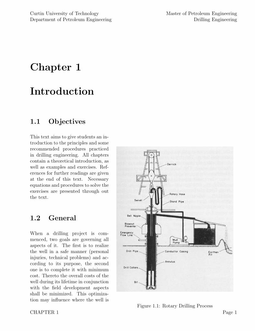
Figure 1.1: Rotary Drilling Process
This text aims to give students an in-troduction to the principles and somerecommended procedures practicedin drilling engineering. All chapterscontain a theoretical introduction, aswell as examples and exercises. Ref-erences for further readings are givenat the end of this text. Necessaryequations and procedures to solve theexercises are presented through outthe text.
1.2 General
When a drilling project is com-menced, two goals are governing allaspects of it. The first is to realizethe well in a safe manner (personalinjuries, technical problems) and ac-cording to its purpose, the secondone is to complete it with minimumcost. Thereto the overall costs of thewell during its lifetime in conjunctionwith the field development aspectsshall be minimized. This optimiza-tion may influence where the well is
CHAPTER 1 Page 1
Curtin University of TechnologyDepartment of Petroleum Engineering
Master of Petroleum EngineeringDrilling Engineering
drilled (onshore - extended reach or offshore above reservoir), the drilling technology applied (con-ventional or slim-hole drilling) as well as which evaluation procedures are run to gather subsurfaceinformation to optimize future wells.
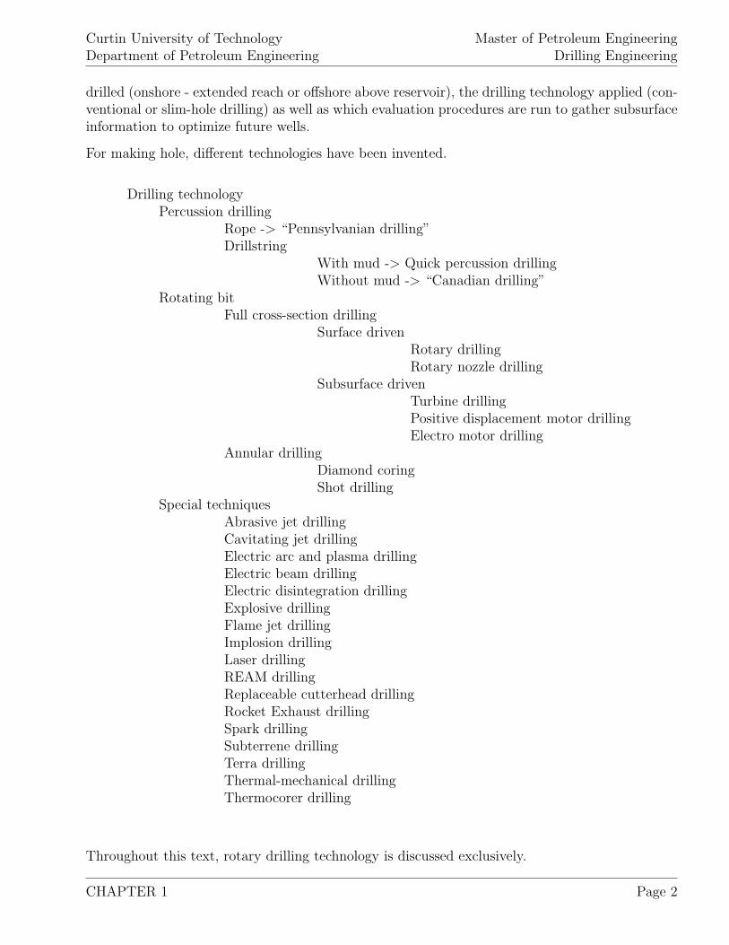
For making hole, different technologies have been invented.
Drilling technologyPercussion drilling
Rope -> “Pennsylvanian drilling”Drillstring
With mud -> Quick percussion drillingWithout mud -> “Canadian drilling”
Rotating bitFull cross-section drilling
Surface drivenRotary drillingRotary nozzle drilling
Subsurface drivenTurbine drillingPositive displacement motor drillingElectro motor drilling
Annular drillingDiamond coringShot drilling
Special techniquesAbrasive jet drillingCavitating jet drillingElectric arc and plasma drillingElectric beam drillingElectric disintegration drillingExplosive drillingFlame jet drillingImplosion drillingLaser drillingREAM drillingReplaceable cutterhead drillingRocket Exhaust drillingSpark drillingSubterrene drillingTerra drillingThermal-mechanical drillingThermocorer drilling
Throughout this text, rotary drilling technology is discussed exclusively.
CHAPTER 1 Page 2
Curtin University of TechnologyDepartment of Petroleum Engineering
Master of Petroleum EngineeringDrilling Engineering
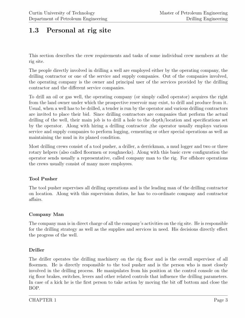
1.3 Personal at rig site
This section describes the crew requirements and tasks of some individual crew members at therig site.
The people directly involved in drilling a well are employed either by the operating company, thedrilling contractor or one of the service and supply companies. Out of the companies involved,the operating company is the owner and principal user of the services provided by the drillingcontractor and the different service companies.
To drill an oil or gas well, the operating company (or simply called operator) acquires the rightfrom the land owner under which the prospective reservoir may exist, to drill and produce from it.Usual, when a well has to be drilled, a tender is run by the operator and various drilling contractorsare invited to place their bid. Since drilling contractors are companies that perform the actualdrilling of the well, their main job is to drill a hole to the depth/location and specifications setby the operator. Along with hiring a drilling contractor ,the operator usually employs variousservice and supply companies to perform logging, cementing or other special operations as well asmaintaining the mud in its planed condition.
Most drilling crews consist of a tool pusher, a driller, a derrickman, a mud logger and two or threerotary helpers (also called floormen or roughnecks). Along with this basic crew configuration theoperator sends usually a representative, called company man to the rig. For offshore operationsthe crews usually consist of many more employees.
Tool Pusher
The tool pusher supervises all drilling operations and is the leading man of the drilling contractoron location. Along with this supervision duties, he has to co-ordinate company and contractoraffairs.
Company Man
The company man is in direct charge of all the company’s activities on the rig site. He is responsiblefor the drilling strategy as well as the supplies and services in need. His decisions directly effectthe progress of the well.
Driller
The driller operates the drilling machinery on the rig floor and is the overall supervisor of allfloormen. He is directly responsible to the tool pusher and is the person who is most closelyinvolved in the drilling process. He manipulates from his position at the control console on therig floor brakes, switches, levers and other related controls that influence the drilling parameters.In case of a kick he is the first person to take action by moving the bit off bottom and close theBOP.
CHAPTER 1 Page 3
Curtin University of TechnologyDepartment of Petroleum Engineering
Master of Petroleum EngineeringDrilling Engineering
Derrick Man
The derrickman works on the so-called monkeyboard, a small platform up in the derrick, usuallyabout 90 [ft] above the rotary table. When a connection is made or during tripping operations heis handling and guiding the upper end of the pipe. During drilling operations the derrickman isresponsible for maintaining and repairing the pumps and other equipment as well as keeping tabson the drilling fluid.
Floor Men
During tripping, the rotary helpers are responsible for handling the lower end of the drill pipe aswell as operating tongs and wrenches to make or break a connection. During other times, theyalso maintain equipment, keep it clean, do painting and in general help where ever help is needed.
Mud Engineer, Mud Logger
The service company who provides the mud almost always sends a mud engineer and a mud loggerto the rig site. They are constantly responsible for logging what is happening in the hole as wellas maintaining the propper mud conditions.
1.4 Miscellaneous
According to a wells final depth, it can be classified into:
Shallow well: < 2,000 [m]
Conventional well: 2,000 [m] - 3,500 [m]
Deep well: 3,500 [m] - 5,000 [m]
Ultra deep well: > 5,000 [m]
With the help of advanced technologies in MWD/LWD and extended reach drilling techniqueshorizontal departures of 10,000+ [m] are possible today (Wytch Farm).
CHAPTER 1 Page 4
Curtin University of TechnologyDepartment of Petroleum Engineering
Master of Petroleum EngineeringDrilling Engineering
Chapter 2
Rotary Drilling Rig
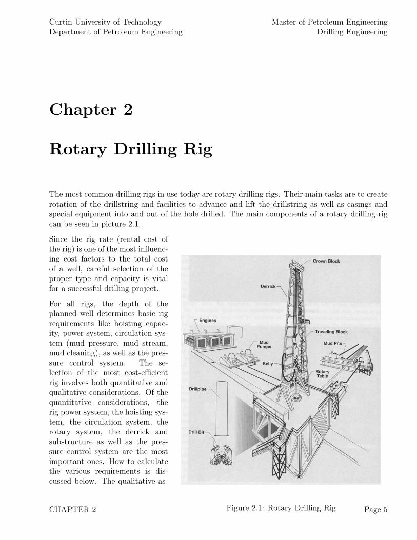
The most common drilling rigs in use today are rotary drilling rigs. Their main tasks are to createrotation of the drillstring and facilities to advance and lift the drillstring as well as casings andspecial equipment into and out of the hole drilled. The main components of a rotary drilling rigcan be seen in picture 2.1.
Figure 2.1: Rotary Drilling Rig
Since the rig rate (rental cost ofthe rig) is one of the most influenc-ing cost factors to the total costof a well, careful selection of theproper type and capacity is vitalfor a successful drilling project.
For all rigs, the depth of theplanned well determines basic rigrequirements like hoisting capac-ity, power system, circulation sys-tem (mud pressure, mud stream,mud cleaning), as well as the pres-sure control system. The se-lection of the most cost-efficientrig involves both quantitative andqualitative considerations. Of thequantitative considerations, therig power system, the hoisting sys-tem, the circulation system, therotary system, the derrick andsubstructure as well as the pres-sure control system are the mostimportant ones. How to calculatethe various requirements is dis-cussed below. The qualitative as-
CHAPTER 2 Page 5
Curtin University of TechnologyDepartment of Petroleum Engineering
Master of Petroleum EngineeringDrilling Engineering
pects involve technical design, appropriate expertise and training of the drilling crew, contractor’strack record and logistics handling.
In general, rotary rigs can be distinguished into:
Land rigs:conventional rigs:
small land rigs,medium land rigs,large land rigs,
mobile rigs:portable mast,jacknife,
Offshore rigs:bottom anchored rigs:
artificial island,TLP,submersible,jackup,concrete-structured, etc.,
floating rigs:drillship,semi-submersible,barge.
For offshore rigs, factors like water depth, expected sea states, winds and currents as well aslocation (supply time) have to be considered as well.
It should be understood that rig rates are not only influenced by the rig type but they are alsostrongly dependent on by the current market situation (oil price, drilling activity, rig availabilities,location, etc.). Therefore for the rig selection basic rig requirements are determined first. Thendrilling contractors are contacted for offers for a proposed spud date (date at which drillingoperation commences) as well as for alternative spud dates. This flexibility to schedule the spuddate may reduce rig rates considerably.
2.1 Rig Power System
The power system of a rotary drilling rig has to supply the following main components: (1) rotarysystem, (2) hoisting system and (3) drilling fluid circulation system. In addition, auxiliaries likethe blowout preventer, boiler-feed water pumps, rig lighting system, etc. have to be powered.Since the largest power consumers on a rotary drilling rig are the hoisting and the circulationsystem, these components determine mainly the total power requirements. At ordinary drilling
CHAPTER 2 Page 6
Curtin University of TechnologyDepartment of Petroleum Engineering
Master of Petroleum EngineeringDrilling Engineering
operations, the hoisting (lifting and lowering of the drillstring, casings, etc.) and the circulationsystem are not operated at the same time. Therefore the same engines can be engaged to performboth functions.
The power itself is either generated at the rig site using internal-combustion diesel engines, ortaken as electric power supply from existing power lines. The raw power is then transmitted tothe operating equipment via: (1) mechanical drives, (2) direct current (DC) or (3) alternatingcurrent (AC) applying a silicon-controlled rectifier (SCR). Most of the newer rigs using the AC-SCR systems. As guideline, power requirements for most rigs are between 1,000 to 3,000 [hp].
The rig power system’s performance is characterised by the output horsepower, torque and fuelconsumption for various engine speeds. These parameters are calculated with equations 2.1 to 2.4:
P =ω.T
33, 000(2.1)
Qi = 0.000393.Wf .ρd.H (2.2)
Et =P
Qi
(2.3)
ω = 2.π.N (2.4)
where:
P [hp] ... shaft power developed by engineω [rad/min] ... angular velocity of the shaftN [rev./min] ... shaft speedT [ft-lbf] ... out-put torqueQi [hp] ... heat energy consumption by engineWf [gal/hr] ... fuel consumptionH [BTU/lbm] ... heating value (diesel: 19,000 [BTU/lbm])Et [1] ... overall power system efficiencyρd [lbm/gal] ... density of fuel (diesel: 7.2 [lbm/gal])33,000 ... conversion factor (ft-lbf/min/hp)
When the rig is operated at environments with non-standard temperatures (85 [F]) or at highaltitudes, the mechanical horsepower requirements have to be modified. This modification isaccording to API standard 7B-11C:
(a) Deduction of 3 % of the standard brake horsepower for each 1,000 [ft] rise
CHAPTER 2 Page 7
Curtin University of TechnologyDepartment of Petroleum Engineering
Master of Petroleum EngineeringDrilling Engineering
in altitude above mean sea level,(b) Deduction of 1 % of the standard brake horsepower for each 10 ◦ rise
or fall in temperature above or below 85 [F], respectively.
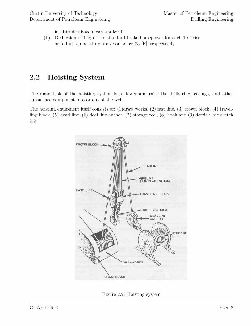
2.2 Hoisting System
The main task of the hoisting system is to lower and raise the drillstring, casings, and othersubsurface equipment into or out of the well.
The hoisting equipment itself consists of: (1)draw works, (2) fast line, (3) crown block, (4) travel-ling block, (5) dead line, (6) deal line anchor, (7) storage reel, (8) hook and (9) derrick, see sketch2.2.
Figure 2.2: Hoisting system
CHAPTER 2 Page 8
Curtin University of TechnologyDepartment of Petroleum Engineering
Master of Petroleum EngineeringDrilling Engineering
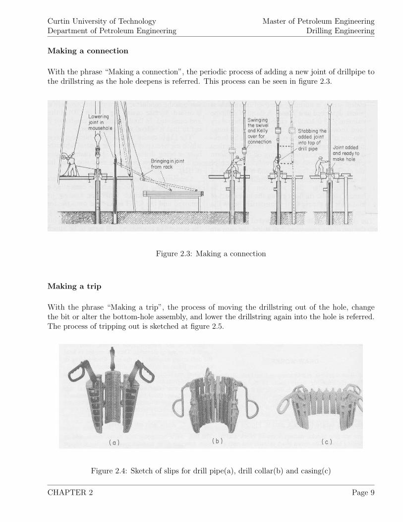
Making a connection
With the phrase “Making a connection”, the periodic process of adding a new joint of drillpipe tothe drillstring as the hole deepens is referred. This process can be seen in figure 2.3.
Figure 2.3: Making a connection
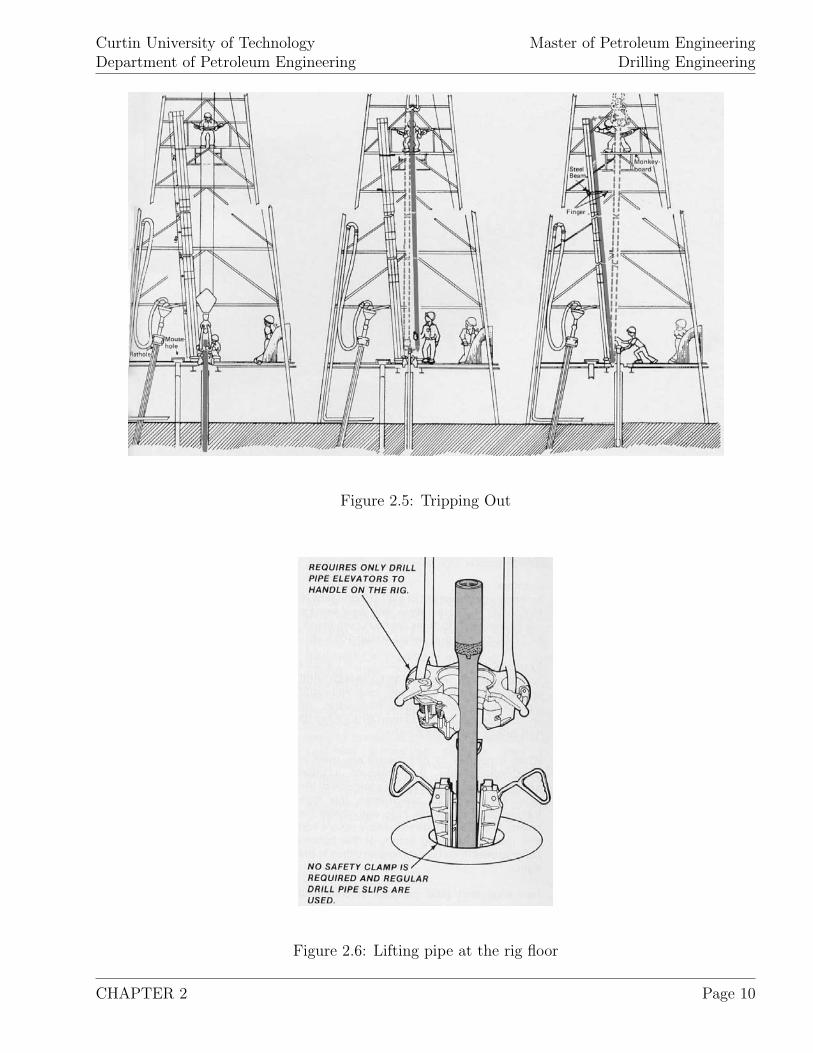
Making a trip
With the phrase “Making a trip”, the process of moving the drillstring out of the hole, changethe bit or alter the bottom-hole assembly, and lower the drillstring again into the hole is referred.The process of tripping out is sketched at figure 2.5.
Figure 2.4: Sketch of slips for drill pipe(a), drill collar(b) and casing(c)
CHAPTER 2 Page 9
Curtin University of TechnologyDepartment of Petroleum Engineering
Master of Petroleum EngineeringDrilling Engineering
Figure 2.5: Tripping Out
Figure 2.6: Lifting pipe at the rig floor
CHAPTER 2 Page 10
Curtin University of TechnologyDepartment of Petroleum Engineering
Master of Petroleum EngineeringDrilling Engineering
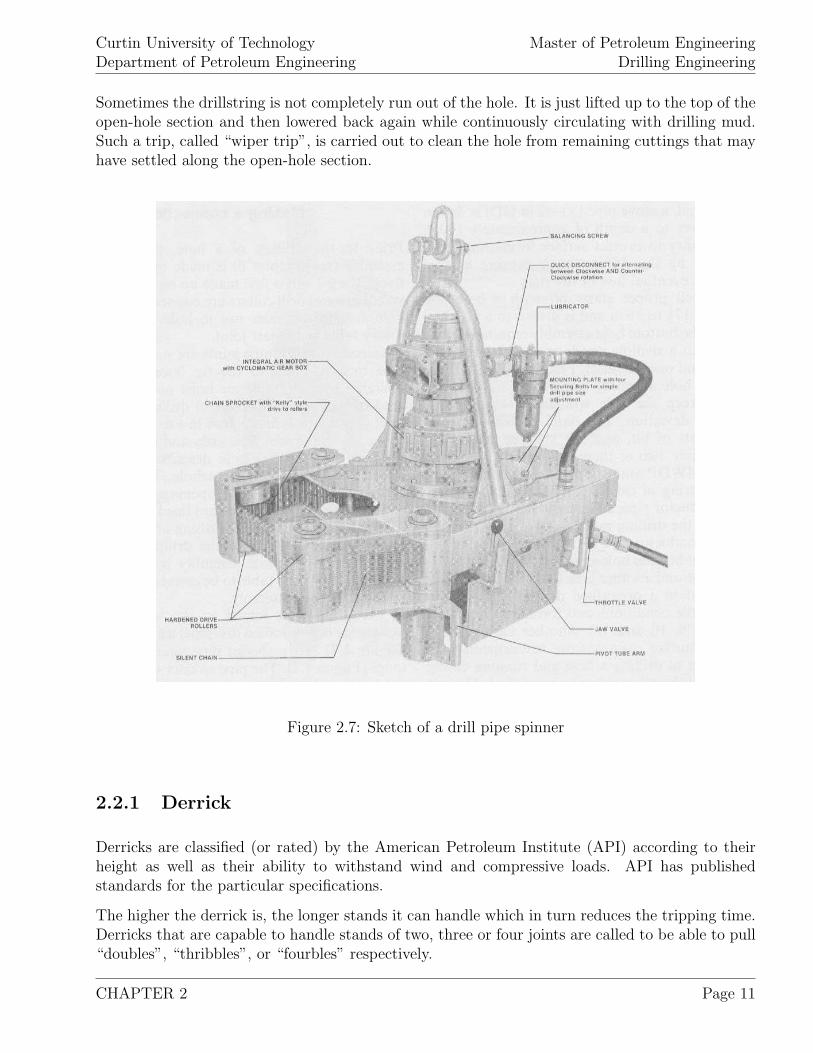
Sometimes the drillstring is not completely run out of the hole. It is just lifted up to the top of theopen-hole section and then lowered back again while continuously circulating with drilling mud.Such a trip, called “wiper trip”, is carried out to clean the hole from remaining cuttings that mayhave settled along the open-hole section.
Figure 2.7: Sketch of a drill pipe spinner
2.2.1 Derrick
Derricks are classified (or rated) by the American Petroleum Institute (API) according to theirheight as well as their ability to withstand wind and compressive loads. API has publishedstandards for the particular specifications.
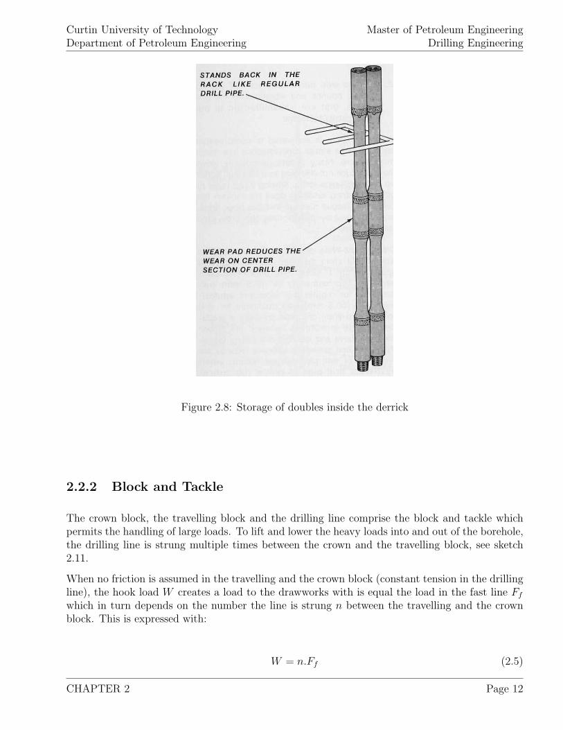
The higher the derrick is, the longer stands it can handle which in turn reduces the tripping time.Derricks that are capable to handle stands of two, three or four joints are called to be able to pull“doubles”, “thribbles”, or “fourbles” respectively.
CHAPTER 2 Page 11
Curtin University of TechnologyDepartment of Petroleum Engineering
Master of Petroleum EngineeringDrilling Engineering
Figure 2.8: Storage of doubles inside the derrick
2.2.2 Block and Tackle
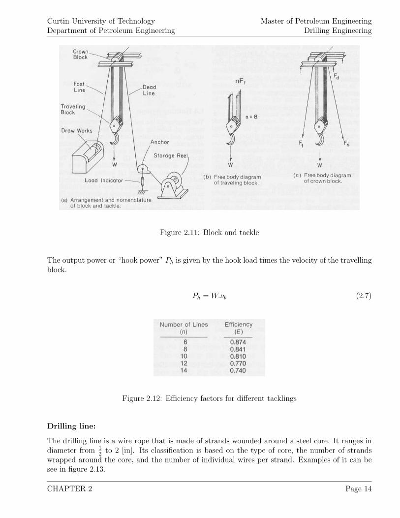
The crown block, the travelling block and the drilling line comprise the block and tackle whichpermits the handling of large loads. To lift and lower the heavy loads into and out of the borehole,the drilling line is strung multiple times between the crown and the travelling block, see sketch2.11.
When no friction is assumed in the travelling and the crown block (constant tension in the drillingline), the hook load W creates a load to the drawworks with is equal the load in the fast line Ff
which in turn depends on the number the line is strung n between the travelling and the crownblock. This is expressed with:
W = n.Ff (2.5)
CHAPTER 2 Page 12
Curtin University of TechnologyDepartment of Petroleum Engineering
Master of Petroleum EngineeringDrilling Engineering
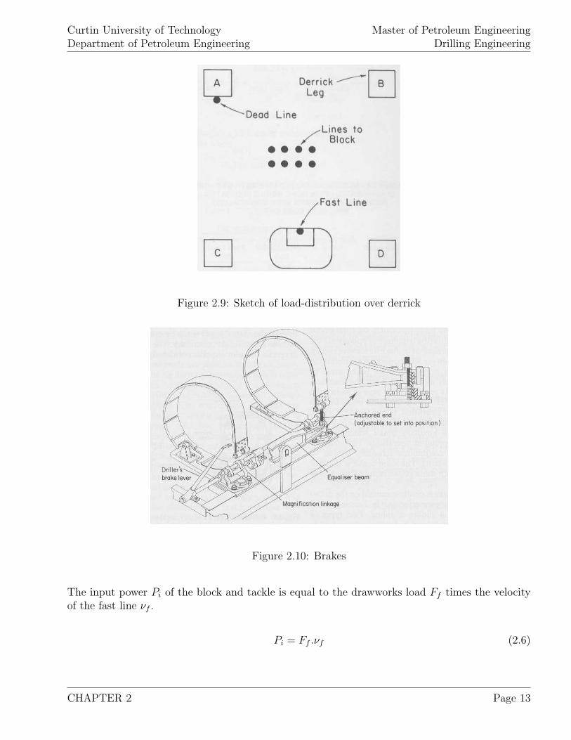
Figure 2.9: Sketch of load-distribution over derrick
Figure 2.10: Brakes
The input power Pi of the block and tackle is equal to the drawworks load Ff times the velocityof the fast line νf .
Pi = Ff .νf (2.6)
CHAPTER 2 Page 13
Curtin University of TechnologyDepartment of Petroleum Engineering
Master of Petroleum EngineeringDrilling Engineering
Figure 2.11: Block and tackle
The output power or “hook power” Ph is given by the hook load times the velocity of the travellingblock.
Ph = W.νb (2.7)
Figure 2.12: Efficiency factors for different tacklings
Drilling line:
The drilling line is a wire rope that is made of strands wounded around a steel core. It ranges indiameter from 1
2to 2 [in]. Its classification is based on the type of core, the number of strands
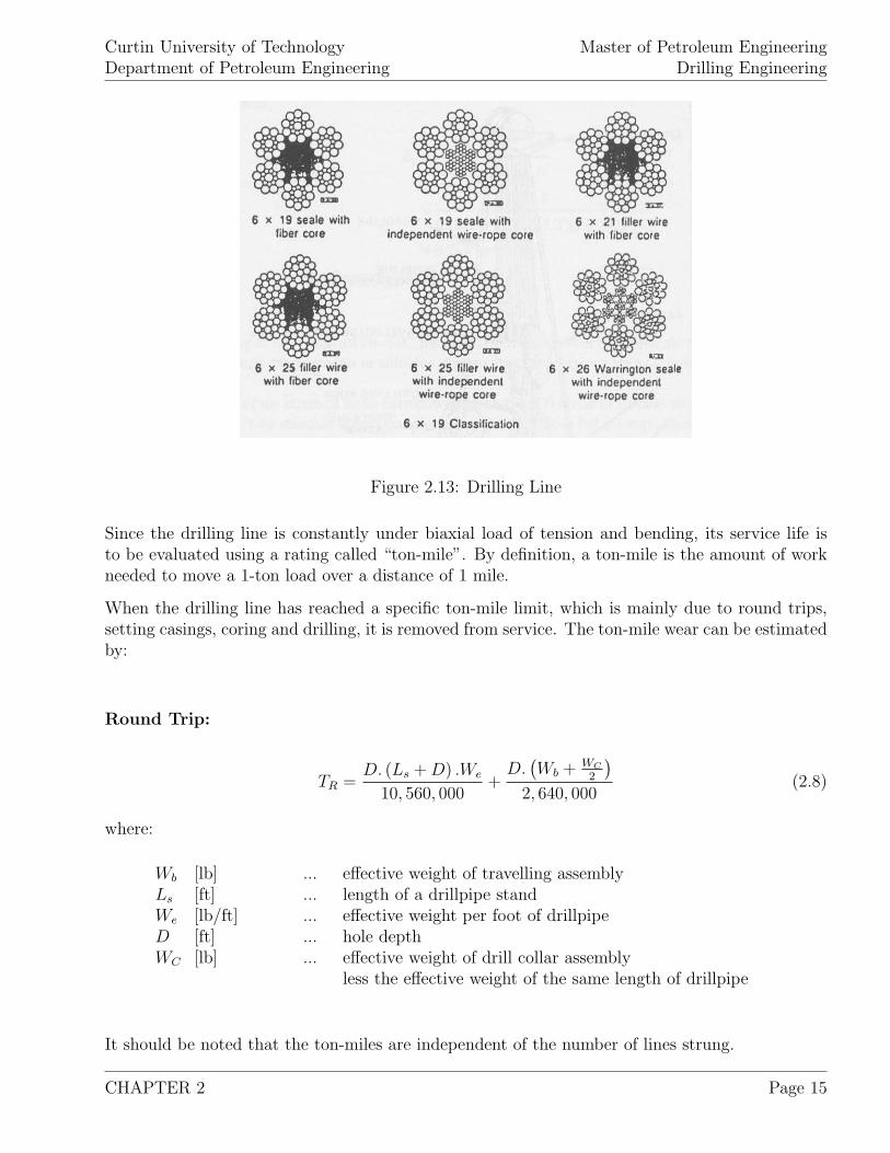
wrapped around the core, and the number of individual wires per strand. Examples of it can besee in figure 2.13.
CHAPTER 2 Page 14
Curtin University of TechnologyDepartment of Petroleum Engineering
Master of Petroleum EngineeringDrilling Engineering
Figure 2.13: Drilling Line
Since the drilling line is constantly under biaxial load of tension and bending, its service life isto be evaluated using a rating called “ton-mile”. By definition, a ton-mile is the amount of workneeded to move a 1-ton load over a distance of 1 mile.
When the drilling line has reached a specific ton-mile limit, which is mainly due to round trips,setting casings, coring and drilling, it is removed from service. The ton-mile wear can be estimatedby:
Round Trip:
TR =D. (Ls + D) .We
10, 560, 000+
D.(Wb + WC
2
)2, 640, 000
(2.8)
where:
Wb [lb] ... effective weight of travelling assemblyLs [ft] ... length of a drillpipe standWe [lb/ft] ... effective weight per foot of drillpipeD [ft] ... hole depthWC [lb] ... effective weight of drill collar assembly
less the effective weight of the same length of drillpipe
It should be noted that the ton-miles are independent of the number of lines strung.
CHAPTER 2 Page 15
Curtin University of TechnologyDepartment of Petroleum Engineering
Master of Petroleum EngineeringDrilling Engineering
The ton-mile service of the drilling line is given for various activities according to:
Drilling operation: (drilling a section from depth d1 to d2) which accounts for:
1. drill ahead a length of kelly
2. pull up length of kelly
3. ream ahead a length of kelly
4. pull up a length of kelly
5. pull kelly in rathole
6. pick up a single (or double)
7. lower drill string in hole
8. pick up kelly and drill ahead
Td = 3. (TR at d2 − TR at d1) (2.9)
Coring operation: which accounts for:
1. core ahead a length of core barrel
2. pull up length of kelly
3. put kelly in rathole
4. pick up a single joint of drillpipe
5. lower drill string in hole
6. pick up kelly
Tc = 2. (TR2 − TR1) (2.10)
where:
TR2 [ton-mile] ... work done for one round trip at depth d2 where coring stoppedTR1 [tin-mile] ... work done for one round trip at depth d1 where coring started.
CHAPTER 2 Page 16
Curtin University of TechnologyDepartment of Petroleum Engineering
Master of Petroleum EngineeringDrilling Engineering
Running Casing:
Tsc = 0.5.
[D. (Lcs + D) .Wcs
10, 560, 000+
D.Wb
2, 640, 000
](2.11)
where:
Lcs [ft] ... length of casing jointWcs [lbm/ft] ... effective weight of casing in mud
The drilling line is subjected to most severe wear at the following two points:
1. The so called “pickup points”, which are at the top of the crown block sheaves and at thebottom of the travelling block sheaves during tripping operations.
2. The so called “lap point”, which is located where a new layer or lap of wire begins on thedrum of the drawworks.
It is common practice that before the entire drilling line is replaced, the location of the pickuppoints and the lap point are varied over different positions of the drilling line by slipping and/orcutting the line.
A properly designed slipping-cut program ensures that the drilling line is maintained in goodcondition and its wear is spread evenly over its length.
To slip the drilling line, the dead-line anchor has to be loosened and a few feet of new line is slippedfrom the storage reel. Cutting off the drilling line requires that the line on the drawworks reelis loosened. Since cutting takes longer and the drawworks reel comprise some additional storage,the drilling line is usually slipped multiple times before it is cut. The length the drilling line isslipped has to be properly calculated so that after slipping, the same part of the line, which wasused before at a pickup point or lap point, is not used again as a pickup point or lap point.
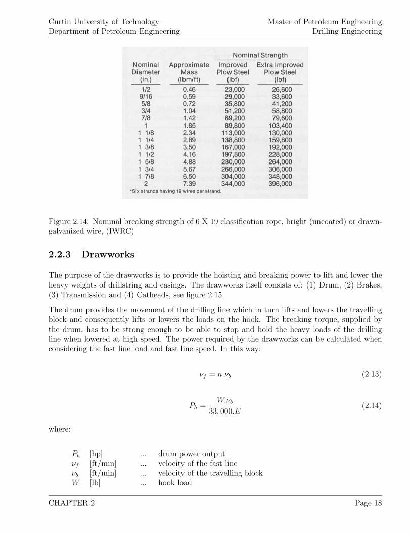
When selecting a drilling line, a “design factor” for the line is applied to compensate for wearand shock loading. API’s recommendation for a minimum design factor (DF ) is 3 for hoistingoperations and 2 for setting casing or pulling on stuck pipe operations. The design factor of thedrilling line is calculated by:
DF =Nominal Strength of Wire Rope [lb]
Fast Line Load [lb](2.12)
CHAPTER 2 Page 17
Curtin University of TechnologyDepartment of Petroleum Engineering
Master of Petroleum EngineeringDrilling Engineering
Figure 2.14: Nominal breaking strength of 6 X 19 classification rope, bright (uncoated) or drawn-galvanized wire, (IWRC)
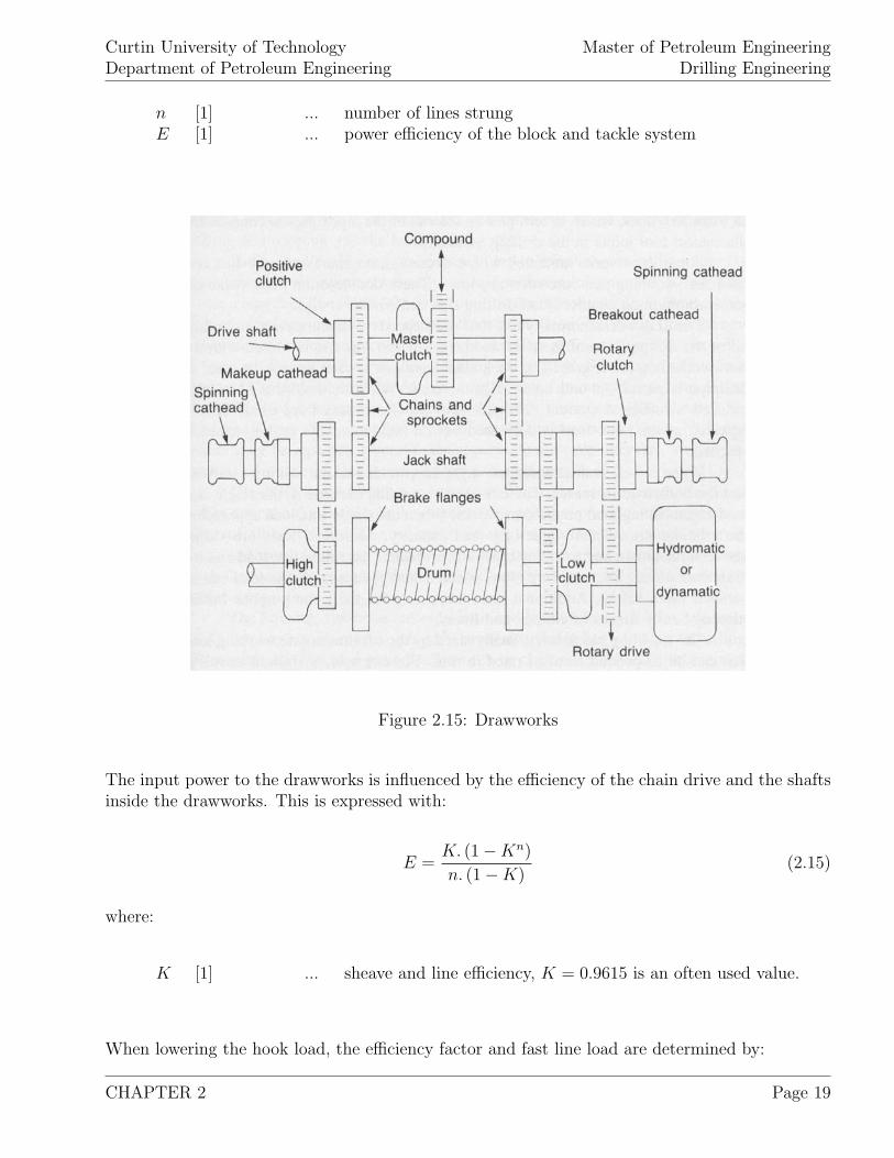
2.2.3 Drawworks
The purpose of the drawworks is to provide the hoisting and breaking power to lift and lower theheavy weights of drillstring and casings. The drawworks itself consists of: (1) Drum, (2) Brakes,(3) Transmission and (4) Catheads, see figure 2.15.
The drum provides the movement of the drilling line which in turn lifts and lowers the travellingblock and consequently lifts or lowers the loads on the hook. The breaking torque, supplied bythe drum, has to be strong enough to be able to stop and hold the heavy loads of the drillingline when lowered at high speed. The power required by the drawworks can be calculated whenconsidering the fast line load and fast line speed. In this way:
νf = n.νb (2.13)
Ph =W.νb
33, 000.E(2.14)
where:
Ph [hp] ... drum power outputνf [ft/min] ... velocity of the fast lineνb [ft/min] ... velocity of the travelling blockW [lb] ... hook load
CHAPTER 2 Page 18
Curtin University of TechnologyDepartment of Petroleum Engineering
Master of Petroleum EngineeringDrilling Engineering
n [1] ... number of lines strungE [1] ... power efficiency of the block and tackle system
Figure 2.15: Drawworks
The input power to the drawworks is influenced by the efficiency of the chain drive and the shaftsinside the drawworks. This is expressed with:
E =K. (1 − Kn)
n. (1 − K)(2.15)
where:
K [1] ... sheave and line efficiency, K = 0.9615 is an often used value.
When lowering the hook load, the efficiency factor and fast line load are determined by:
CHAPTER 2 Page 19
Curtin University of TechnologyDepartment of Petroleum Engineering
Master of Petroleum EngineeringDrilling Engineering
ELowering =n.Kn. (1 − K)
1 − Kn(2.16)
Ff−Lowering =W.K−n. (1 − K)
1 − Kn(2.17)
where:
Ff [lbf] ... tension in the fast line
2.3 Rig Selection
Following parameters are used to determine the minimum criteria to select a suitable drilling rig:
(1) Static tension in the fast line when upward motion is impending(2) Maximum hook horsepower(3) Maximum hoisting speed(4) Actual derrick load(5) Maximum equivalent derrick load(6) Derrick efficiency factor
They can be calculated by following equations:
Pi = Ff .νf (2.18)
νb =Ph
W(2.19)
Fd =1 + E + E.n
E.n.W (2.20)
Fde =
(n + 4
n
).W (2.21)
Ed =Fd
Fde
=E.(n + 1) + 1
E.(n + 4)(2.22)
where:
CHAPTER 2 Page 20

Curtin University of TechnologyDepartment of Petroleum Engineering
Master of Petroleum EngineeringDrilling Engineering
Fd [lbf] ... load applied to derrick, sum of the hook load,tension in the dead line and tension in the fast line
Fde [lbf] ... maximum equivalent derrick load, equal tofour times the maximum leg load
Ed [1] ... derrick efficiency factor
CHAPTER 2 Page 21
Curtin University of TechnologyDepartment of Petroleum Engineering
Master of Petroleum EngineeringDrilling Engineering
2.4 Circulation System
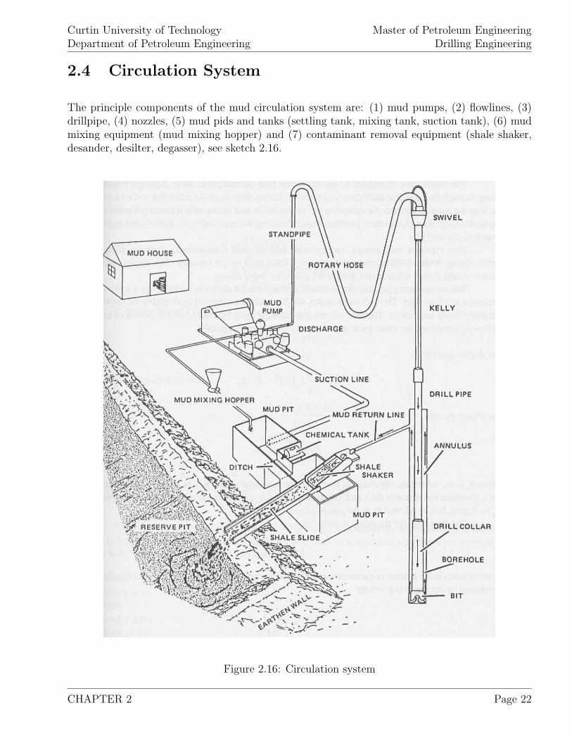
The principle components of the mud circulation system are: (1) mud pumps, (2) flowlines, (3)drillpipe, (4) nozzles, (5) mud pids and tanks (settling tank, mixing tank, suction tank), (6) mudmixing equipment (mud mixing hopper) and (7) contaminant removal equipment (shale shaker,desander, desilter, degasser), see sketch 2.16.
Figure 2.16: Circulation system
CHAPTER 2 Page 22
Curtin University of TechnologyDepartment of Petroleum Engineering
Master of Petroleum EngineeringDrilling Engineering
The flow of circulated drilling mud can be described as from the mud pit (storage of mud) via themud mixing hopper, where various additives like weighting material etc. can be mixed into themud, or the suction line to the mud pumps. At the mud pumps the mud is pressured up to therequired mud pressure value. From the mud pumps the mud is pushed through the stand pipe (apipe fixed mounted at the derrick), the rotary hose (flexible connection that allows the fed of themud into the vertically moving drillstring), via the swivel into the drillstring. Inside the drillstring(kelly, drillpipe, drill collar) the mud flows down to the bit where it is forced through the nozzlesto act against the bottom of the hole. From the bottom of the well the mud rises up the annuli(drill collar, drillpipe) and the mud line (mud return line) which is located above the BOP. Fromthe mud line the mud is fed to the mud cleaning system consisting of shale shakers, settlementtank, de-sander and de-silter. After cleaning the mud, the circulation circle is closed when themud returns to the mud pit.
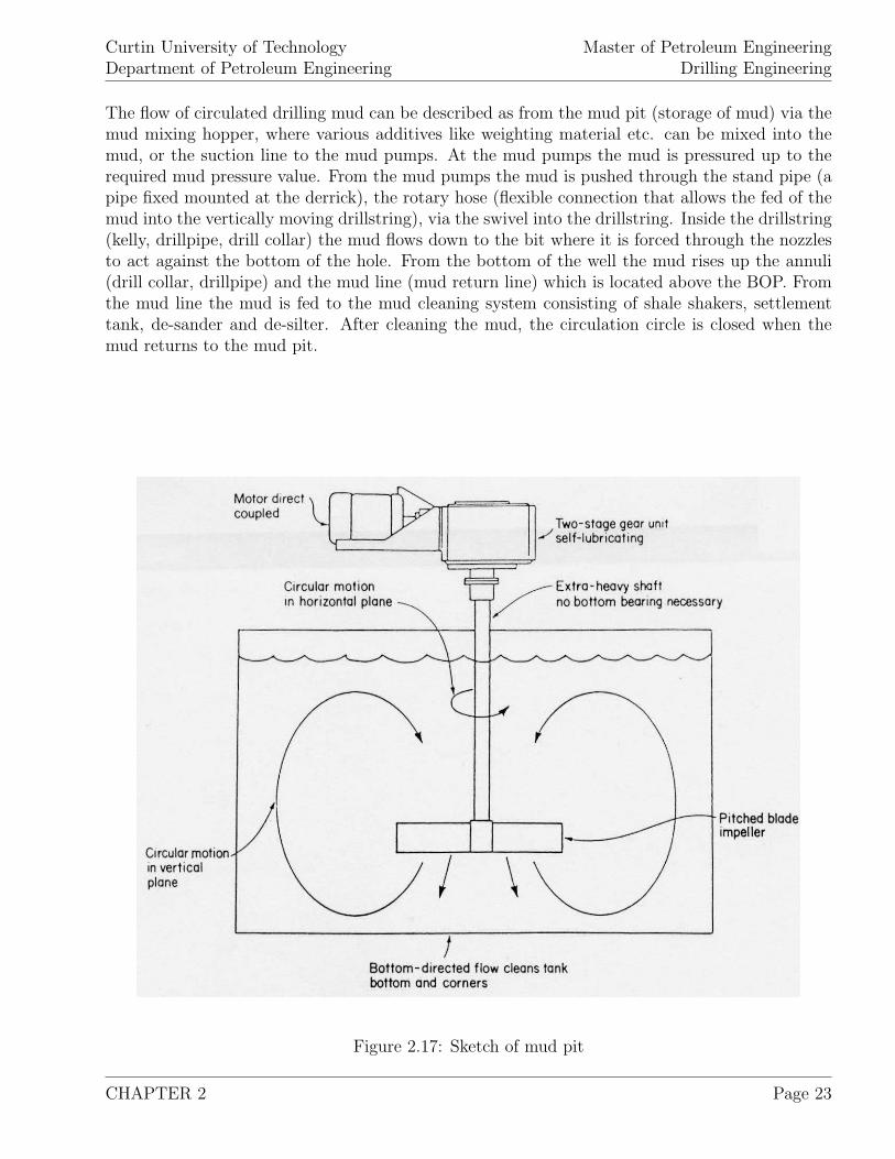
Figure 2.17: Sketch of mud pit
CHAPTER 2 Page 23
Curtin University of TechnologyDepartment of Petroleum Engineering
Master of Petroleum EngineeringDrilling Engineering
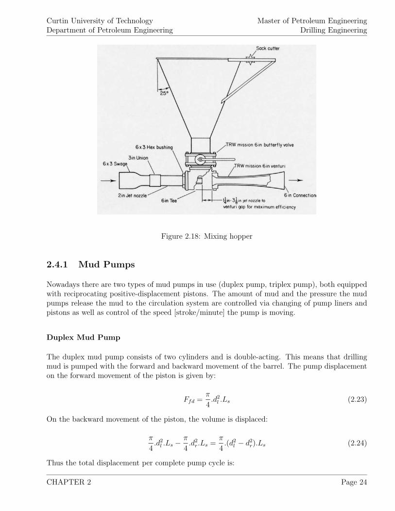
Figure 2.18: Mixing hopper
2.4.1 Mud Pumps
Nowadays there are two types of mud pumps in use (duplex pump, triplex pump), both equippedwith reciprocating positive-displacement pistons. The amount of mud and the pressure the mudpumps release the mud to the circulation system are controlled via changing of pump liners andpistons as well as control of the speed [stroke/minute] the pump is moving.
Duplex Mud Pump
The duplex mud pump consists of two cylinders and is double-acting. This means that drillingmud is pumped with the forward and backward movement of the barrel. The pump displacementon the forward movement of the piston is given by:
Ffd =π
4.d2
l .Ls (2.23)
On the backward movement of the piston, the volume is displaced:
π
4.d2
l .Ls − π
4.d2
r.Ls =π
4.(d2
l − d2r).Ls (2.24)
Thus the total displacement per complete pump cycle is:
CHAPTER 2 Page 24
Curtin University of TechnologyDepartment of Petroleum Engineering
Master of Petroleum EngineeringDrilling Engineering
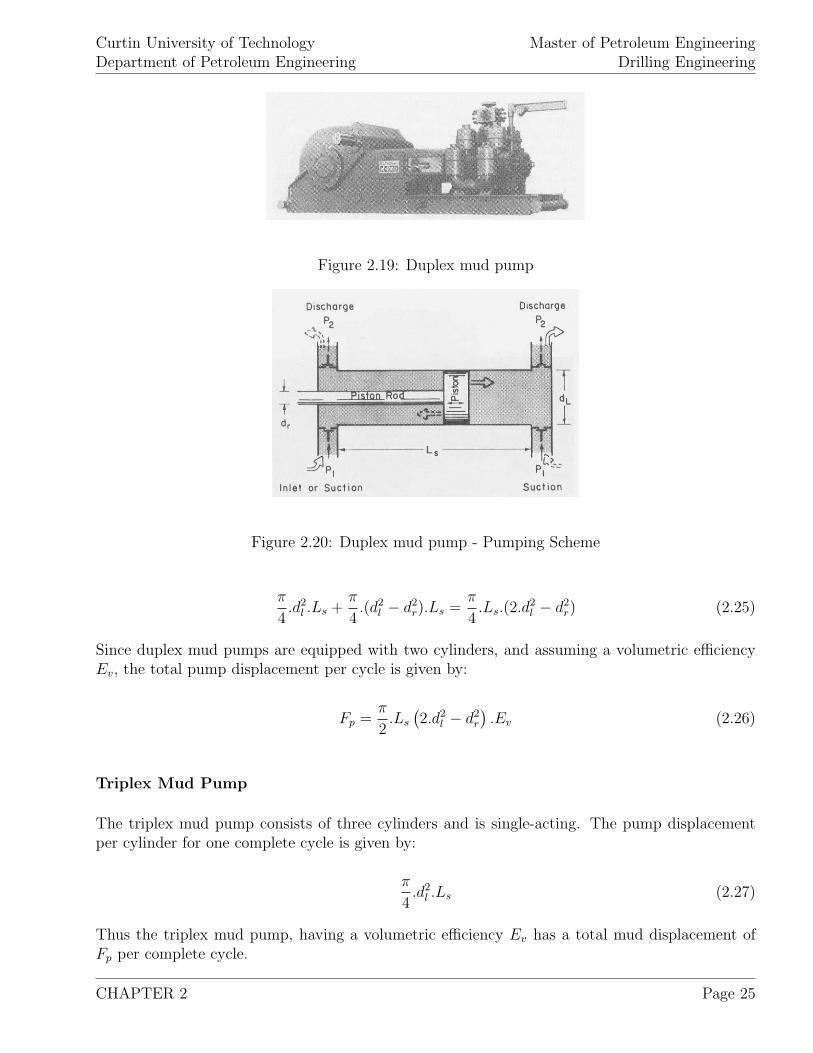
Figure 2.19: Duplex mud pump
Figure 2.20: Duplex mud pump - Pumping Scheme
π
4.d2
l .Ls +π
4.(d2
l − d2r).Ls =
π
4.Ls.(2.d
2l − d2
r) (2.25)
Since duplex mud pumps are equipped with two cylinders, and assuming a volumetric efficiencyEv, the total pump displacement per cycle is given by:
Fp =π
2.Ls
(2.d2
l − d2r
).Ev (2.26)
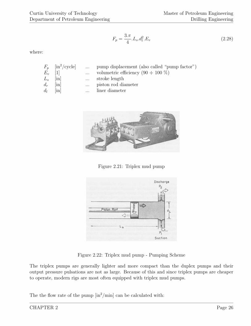
Triplex Mud Pump
The triplex mud pump consists of three cylinders and is single-acting. The pump displacementper cylinder for one complete cycle is given by:
π
4.d2
l .Ls (2.27)
Thus the triplex mud pump, having a volumetric efficiency Ev has a total mud displacement ofFp per complete cycle.
CHAPTER 2 Page 25
Curtin University of TechnologyDepartment of Petroleum Engineering
Master of Petroleum EngineeringDrilling Engineering
Fp =3.π
4.Ls.d
2l .Ev (2.28)
where:
Fp [in2/cycle] ... pump displacement (also called “pump factor”)Ev [1] ... volumetric efficiency (90 ÷ 100 %)Ls [in] ... stroke lengthdr [in] ... piston rod diameterdl [in] ... liner diameter
Figure 2.21: Triplex mud pump
Figure 2.22: Triplex mud pump - Pumping Scheme
The triplex pumps are generally lighter and more compact than the duplex pumps and theiroutput pressure pulsations are not as large. Because of this and since triplex pumps are cheaperto operate, modern rigs are most often equipped with triplex mud pumps.
The the flow rate of the pump [in2/min] can be calculated with:
CHAPTER 2 Page 26
Curtin University of TechnologyDepartment of Petroleum Engineering
Master of Petroleum EngineeringDrilling Engineering
q = N.Fp (2.29)
where:
N [cycles/min] ... number of cycles per minute
The overall efficiency of a mud pump is the product of the mechanical and the volumetric efficiency.The mechanical efficiency is often assumed to be 90% and is related to the efficiency of the primemover itself and the linkage to the pump drive shaft. The volumetric efficiency of a mud pumpwith adequately charged suction system can be as high as 100%. Therefore most manufacturesrate their pumps with a total efficiency of 90% (mechanical efficiency: 90%, volumetric efficiency:100%).
Note that per revolution, the duplex pump makes two cycles (double-acting) where the triplexpump completes one cycle (single-acting).
The terms “cycle” and “stroke” are applied interchangeably in the industry and refer to onecomplete pump revolution.
Pumps are generally rated according to their:
1. Hydraulic power,
2. Maximum pressure,
3. Maximum flow rate.
Since the inlet pressure is essentially atmospheric pressure, the increase of mud pressure due tothe mud pump is approximately equal the discharge pressure.
The hydraulic power [hp] provided by the mud pump can be calculated as:
PH =∆p.q
1, 714(2.30)
where:
∆p [psi] ... pump discharge pressureq [gal/min] ... pump discharge flow rate
CHAPTER 2 Page 27
Curtin University of TechnologyDepartment of Petroleum Engineering
Master of Petroleum EngineeringDrilling Engineering
At a given hydraulic power level, the maximum discharge pressure and the flow rate can be variedby changing the stroke rate as well as the liner seize. A smaller liner will allow the operator toobtain a higher pump pressure but at a lower flow rate. Pressures above 3,500 [psi] are appliedseldomly since they cause a significant increase in maintenance problems.
In practice, especially at shallow, large diameter section, more pumps are often used simultaneouslyto feed the mud circulation system with the required total mud flow and intake pressure. For thisreason the various mud pumps are connected in parallel and operated with the same outputpressure. The individual mud streams are added to compute the total one.
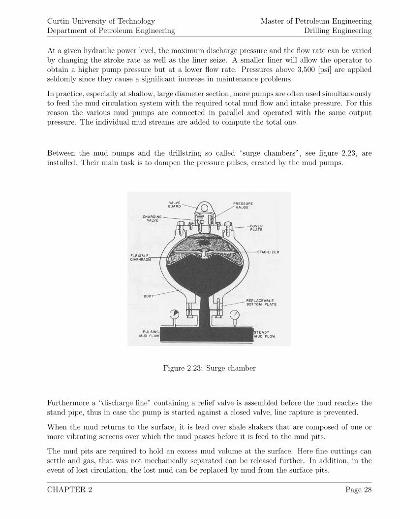
Between the mud pumps and the drillstring so called “surge chambers”, see figure 2.23, areinstalled. Their main task is to dampen the pressure pulses, created by the mud pumps.
Figure 2.23: Surge chamber
Furthermore a “discharge line” containing a relief valve is assembled before the mud reaches thestand pipe, thus in case the pump is started against a closed valve, line rapture is prevented.
When the mud returns to the surface, it is lead over shale shakers that are composed of one ormore vibrating screens over which the mud passes before it is feed to the mud pits.
The mud pits are required to hold an excess mud volume at the surface. Here fine cuttings cansettle and gas, that was not mechanically separated can be released further. In addition, in theevent of lost circulation, the lost mud can be replaced by mud from the surface pits.
CHAPTER 2 Page 28
Curtin University of TechnologyDepartment of Petroleum Engineering
Master of Petroleum EngineeringDrilling Engineering
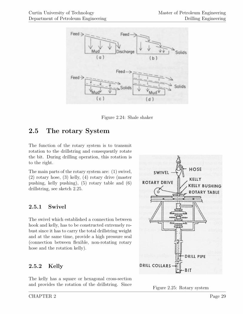
Figure 2.24: Shale shaker
2.5 The rotary System
Figure 2.25: Rotary system
The function of the rotary system is to transmitrotation to the drillstring and consequently rotatethe bit. During drilling operation, this rotation isto the right.
The main parts of the rotary system are: (1) swivel,(2) rotary hose, (3) kelly, (4) rotary drive (masterpushing, kelly pushing), (5) rotary table and (6)drillstring, see sketch 2.25.
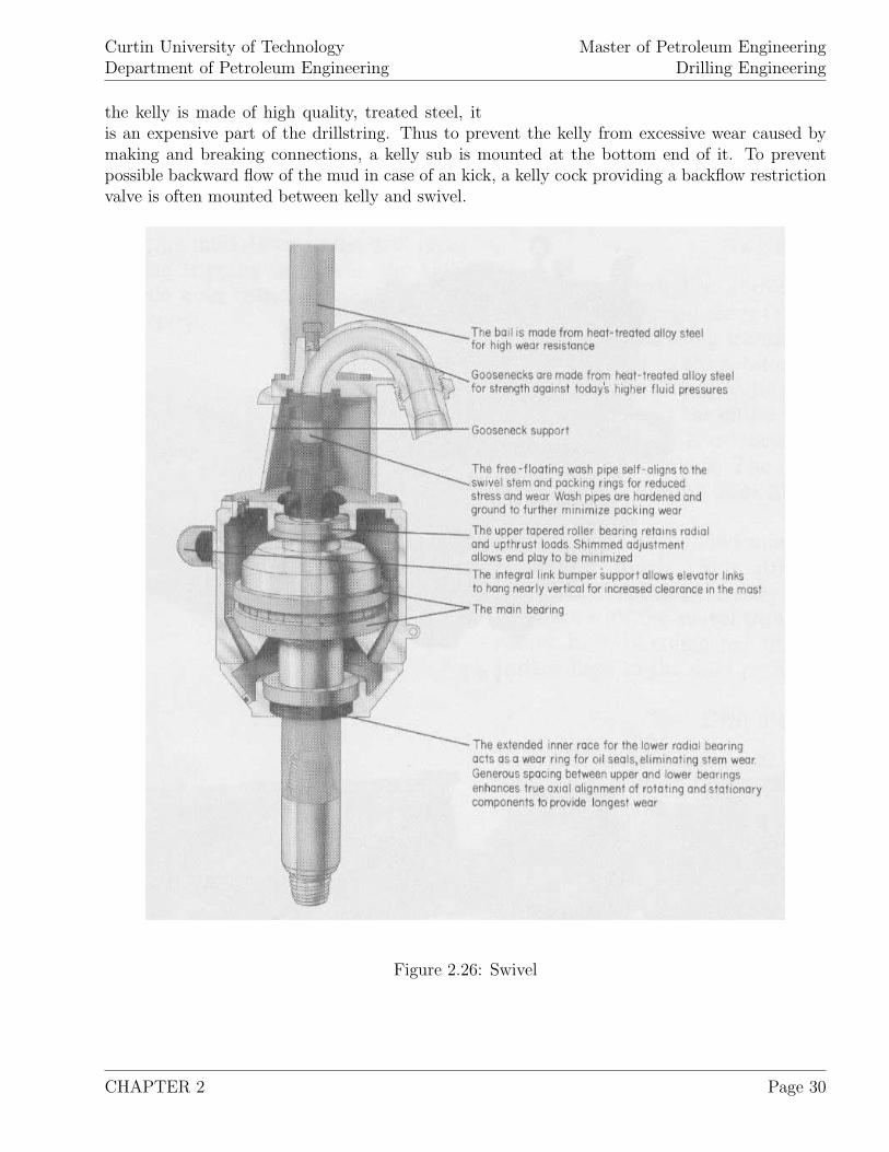
2.5.1 Swivel
The swivel which established a connection betweenhook and kelly, has to be constructed extremely ro-bust since it has to carry the total drillstring weightand at the same time, provide a high pressure seal(connection between flexible, non-rotating rotaryhose and the rotation kelly).
2.5.2 Kelly
The kelly has a square or hexagonal cross-sectionand provides the rotation of the drillstring. Since
CHAPTER 2 Page 29
Curtin University of TechnologyDepartment of Petroleum Engineering
Master of Petroleum EngineeringDrilling Engineering
the kelly is made of high quality, treated steel, itis an expensive part of the drillstring. Thus to prevent the kelly from excessive wear caused bymaking and breaking connections, a kelly sub is mounted at the bottom end of it. To preventpossible backward flow of the mud in case of an kick, a kelly cock providing a backflow restrictionvalve is often mounted between kelly and swivel.
Figure 2.26: Swivel
CHAPTER 2 Page 30
Curtin University of TechnologyDepartment of Petroleum Engineering
Master of Petroleum EngineeringDrilling Engineering
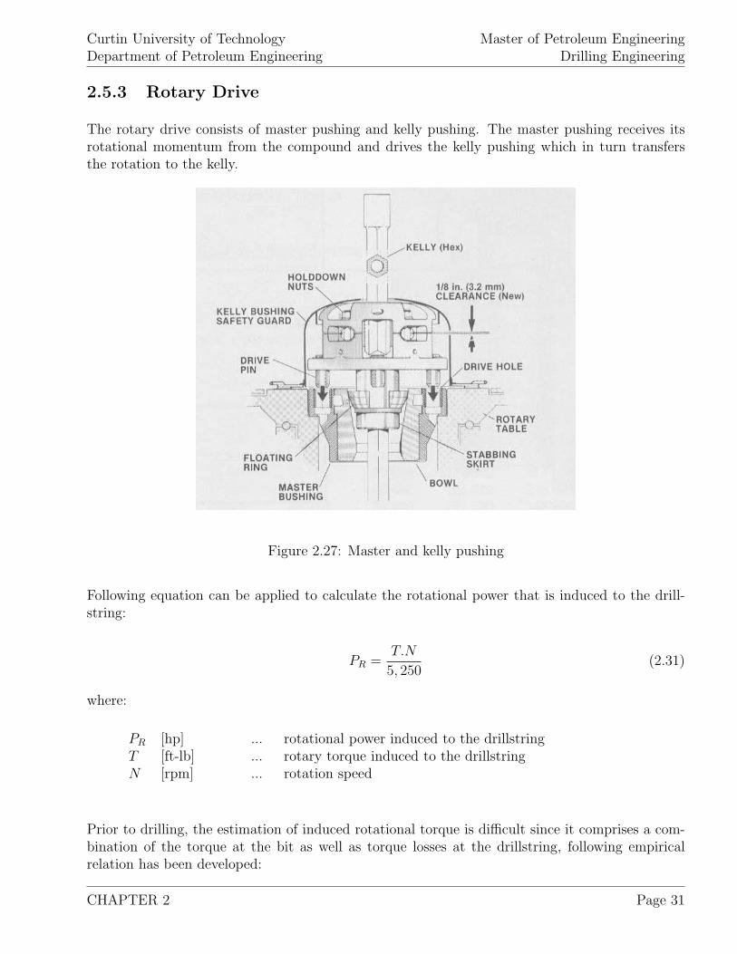
2.5.3 Rotary Drive
The rotary drive consists of master pushing and kelly pushing. The master pushing receives itsrotational momentum from the compound and drives the kelly pushing which in turn transfersthe rotation to the kelly.
Figure 2.27: Master and kelly pushing
Following equation can be applied to calculate the rotational power that is induced to the drill-string:
PR =T.N
5, 250(2.31)
where:
PR [hp] ... rotational power induced to the drillstringT [ft-lb] ... rotary torque induced to the drillstringN [rpm] ... rotation speed
Prior to drilling, the estimation of induced rotational torque is difficult since it comprises a com-bination of the torque at the bit as well as torque losses at the drillstring, following empiricalrelation has been developed:
CHAPTER 2 Page 31
Curtin University of TechnologyDepartment of Petroleum Engineering
Master of Petroleum EngineeringDrilling Engineering
PR = F.N (2.32)
The torque factor is approximated with 1.5 for wells with MD smaller than 10,000 [ft], 1.75 forwells with MD of 10,000 to 15,000 [ft] and 2.0 for wells with MD larger than 15,000 [ft].
The volume contained and displaced by the drillstring can be calculated as:
Capacity of drillpipe or drill collar:
Vp =d2
1, 029.4(2.33)
Capacity of the annulus behind drillpipe or drill collar:
Va =(d2
2 − d21)
1, 029.4(2.34)
Displacement of drillpipe or drill collar:
Vs =(d2
1 − d2)
1, 029.4(2.35)
where:
d [in] ... inside diameter of drillpipe or drill collard1 [in] ... outside diameter of drillpipe or drill collard2 [in] ... hole diameterV [bbl/ft] ... capacity of drillpipe, collar or annulus
2.6 Drilling Cost Analysis
To estimate the cost of realizing a well as well as to perform economical evaluation of the drillingproject, before commencing the project, a so called AFE (Authority For Expenditure) has to beprepared and signed of by the operator. Within the AFE all cost items are listed as they areknown or can be estimated at the planning stage. During drilling, a close follow up of the actualcost and a comparison with the estimated (and authorized) ones are done on a daily bases.
When preparing an AFE, different completions and objectives (dry hole, with casing and comple-tion, etc) can be included to cost-estimate different scenarios.
Generally, an AFE consists of the following major groups:
CHAPTER 2 Page 32
Curtin University of TechnologyDepartment of Petroleum Engineering
Master of Petroleum EngineeringDrilling Engineering
(1) Wellsite preparation,(2) Rig mobilization and rigging up,(3) Rig Rental,(4) Drilling Mud,(5) Bits and Tools,(6) Casings,(7) Formation evaluation
The listed cost items and their spread are different at each company and can be different withinone company (onshore-offshore, various locations, etc.).
Along with the well plan (well proposal) a operational schedule as well as a schedule of expecteddaily costs has to be prepared.
In the following simple methods to estimate the drilling costs as well as, the drilling and trippingtimes are given.
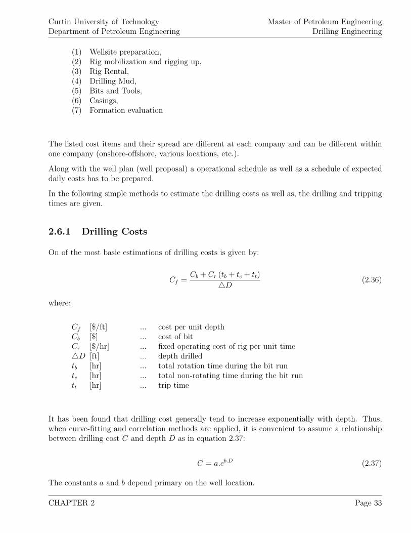
2.6.1 Drilling Costs
On of the most basic estimations of drilling costs is given by:
Cf =Cb + Cr (tb + tc + tt)
�D(2.36)
where:
Cf [$/ft] ... cost per unit depthCb [$] ... cost of bitCr [$/hr] ... fixed operating cost of rig per unit time�D [ft] ... depth drilledtb [hr] ... total rotation time during the bit runtc [hr] ... total non-rotating time during the bit runtt [hr] ... trip time
It has been found that drilling cost generally tend to increase exponentially with depth. Thus,when curve-fitting and correlation methods are applied, it is convenient to assume a relationshipbetween drilling cost C and depth D as in equation 2.37:
C = a.eb.D (2.37)
The constants a and b depend primary on the well location.
CHAPTER 2 Page 33
Curtin University of TechnologyDepartment of Petroleum Engineering
Master of Petroleum EngineeringDrilling Engineering
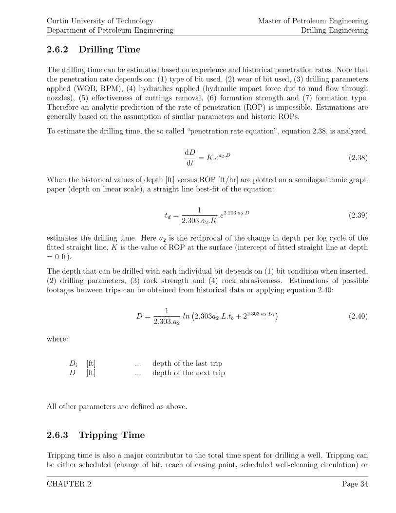
2.6.2 Drilling Time
The drilling time can be estimated based on experience and historical penetration rates. Note thatthe penetration rate depends on: (1) type of bit used, (2) wear of bit used, (3) drilling parametersapplied (WOB, RPM), (4) hydraulics applied (hydraulic impact force due to mud flow throughnozzles), (5) effectiveness of cuttings removal, (6) formation strength and (7) formation type.Therefore an analytic prediction of the rate of penetration (ROP) is impossible. Estimations aregenerally based on the assumption of similar parameters and historic ROPs.
To estimate the drilling time, the so called “penetration rate equation”, equation 2.38, is analyzed.
dD
dt= K.ea2.D (2.38)
When the historical values of depth [ft] versus ROP [ft/hr] are plotted on a semilogarithmic graphpaper (depth on linear scale), a straight line best-fit of the equation:
td =1
2.303.a2.K.e2.203.a2.D (2.39)
estimates the drilling time. Here a2 is the reciprocal of the change in depth per log cycle of thefitted straight line, K is the value of ROP at the surface (intercept of fitted straight line at depth= 0 ft).
The depth that can be drilled with each individual bit depends on (1) bit condition when inserted,(2) drilling parameters, (3) rock strength and (4) rock abrasiveness. Estimations of possiblefootages between trips can be obtained from historical data or applying equation 2.40:
D =1
2.303.a2
.ln(2.303a2.L.tb + 22.303.a2.Di
)(2.40)
where:
Di [ft] ... depth of the last tripD [ft] ... depth of the next trip
All other parameters are defined as above.
2.6.3 Tripping Time
Tripping time is also a major contributor to the total time spent for drilling a well. Tripping canbe either scheduled (change of bit, reach of casing point, scheduled well-cleaning circulation) or
CHAPTER 2 Page 34
Curtin University of TechnologyDepartment of Petroleum Engineering
Master of Petroleum EngineeringDrilling Engineering
on-scheduled, due to troubles. Types of troubles, their origin and possible actions are discussedin a later chapter.
Following relationship can be applied to estimate the tripping time to change the bit. Thus theoperations of trip out, change bit, trip in are included:
tt = 2.
(tsls
.D
)(2.41)
where:
tt [hr] ... required time for round tripts [hr] ... average time required to handle one standD [ft or m] ... length of drillstring to tripls [ft or m] ... average length of one stand
The term “stand” refers to the joints of drillpipe left connected and placed inside the derrickduring tripping. Depending on the derrick seize, one stand consists mostly of three, sometimesfour drillpipes. In this way during tripping only each third (fourth) connection has to be brokenand made up for tripping.
CHAPTER 2 Page 35
Curtin University of TechnologyDepartment of Petroleum Engineering
Master of Petroleum EngineeringDrilling Engineering
2.7 Examples
1. The output torque and speed of a diesel engine is 1,650 [ft-lbf] and 800 [rpm] respectively.Calculate the brake horsepower and overall engine efficiency when the diesel consumption rate is15.7 [gal/hr]. What is the fuel consumption for a 24 hr working day?
2. When drilling at 7,000 [ft] with an assembly consisting of 500 [ft] drill collars (8 [in] OD, 2.5[in] ID, 154 [lbm/ft]) on a 5 [in], 19.5 [lbm/ft] , a 10.0 [ppg] drilling mud is used. What are theton-miles applying following assumptions (one joint of casing is 40 [ft], travelling block assemblyweights 28,000 [lbm], each stand is 93 [ft] long) when:
(a) Running 7 [in], 29 [lbm/ft] casing,(b) Coring from 7,000 [ft] to 7,080 [ft],(c) Drilling from 7,000 [ft] to 7,200 [ft],(d) Making a round-trip at 7,000 [ft]?
3. The rig’s drawworks can provide a maximum power of 800 [hp]. To lift the calculated load of200,000 [lb], 10 lines are strung between the crown block and the traveling block. The lead line isanchored to a derrick leg on one side of the v-door. What is the:
(a) Static tension in the fast line,(b) Maximum hook horsepower available,(c) Maximum hoisting speed,(d) Derrick load when upward motion is impending,(e) Maximum equivalent derrick load,(f) Derrick efficiency factor?
4. After circulation the drillstring is recognized to be stuck. For pulling the drillstring, followingequipment data have to be considered: derrick can support a maximum equivalent derrick load of500,000 [lbf], the drilling line strength is 51,200 [lbf], the maximum tension load of the drillpipeis 396,000 [lbf]. 8 lines are strung between the crown block and the traveling block, for pulling tofree the stuck pipe, a safety factor of 2.0 is to be applied for the derrick, the drillpipe as well asthe drilling line. What is the maximum force the driller can pull to try to free the pipe?
5. To run 425,000 [lb] of casing on a 10-line system, a 1.125 [in], 6x19 extra improved plow steeldrilling line is used. When K is assumed to be 0.9615, does this configuration meet a safety factorrequirement for the ropes of 2.0? What is the maximum load that can be run meeting the safetyfactor?
CHAPTER 2 Page 36
Curtin University of TechnologyDepartment of Petroleum Engineering
Master of Petroleum EngineeringDrilling Engineering
6. A drillstring of 300,000 [lb] is used in a well where the rig has sufficient horsepower to runthe string at a minimum rate of 93 [ft/min]. The hoisting system has 8 lines between the crownblock and the travelling block, the mechanical drive of the rig has following configuration: Engineno. 1: (4 shafts, 3 chains), engine no. 2: (5 shafts, 4 chains), engine no. 3: (6 shafts, 5 chains).Thus the total elements of engine 1 is 7, of engine 2 9 and of engine 3 11. When the efficiencies ofeach shaft, chain and sheave pair is 0.98 and 0.75 for the torque converter, what is the minimumacceptable input horsepower and fast line velocity?
7. A triplex pump is operating at 120 [cycles/min] and discharging the mud at 3,000 [psig]. Whenthe pump has installed a 6 [in] liner operating with 11 [in] strokes, what are the:
(a) Pump factor in [gal/cycles] when 100 %volumetric efficiency is assumed,
(b) Flow rate in [gal/min],(c) Pump power development?
8. A drillstring consists of 9,000 [ft] 5 [in], 19,5 [lbm/ft] drillpipe, and 1,000 [ft] of 8 [in] OD, 3[in] ID drill collars. What is the:
(a) Capacity of the drillpipe in [bbl],(b) Capacity of the drill collars in [bbl],(c) Number of pump cycles required to pump surface mud to the bit
(duplex pump, 6 [in] liners, 2.5 [in] rods, 16 [in] strokes,pumping at 85 % volumetric efficiency),
(d) Displacement of drillpipes in [bbl/ft],(e) Displacement of drill collars in [bbl/ft],(f) Loss in fluid level in the hole if 10 stands (thribbles) drillpipe
are pulled without filling the hole (casing 10.05 [in] ID),(g) Change in fluid level in the pit when the hole is filled after
pulling 10 stands of drillpipe. The pit is 8 [ft] wide and20 [ft] long.
9. A diesel engine gives an output torque of 1,740 [ft-lbf] at an engine speed of 1,200 [rpm]. Therig is operated in Mexico at an altitude of 1,430 [ft] above MSL at a average temperature of 28◦C. When the fuel consumption rate is 31.8 [gal/hr], what is the output power and the overallefficiency of the engine?
10. A rig must hoist a load of 320,000 [lb]. The drawworks can provide an input power to theblock and tackle system as high as 500 [hp]. Eight lines are strung between the crown block andthe travelling block. Calculate:
CHAPTER 2 Page 37
Curtin University of TechnologyDepartment of Petroleum Engineering
Master of Petroleum EngineeringDrilling Engineering
(a) Static tension in the fast line,(b) Maximum hook horse power,(c) Maximum hoisting speed,(d) Effective derrick load,(e) Maximum equivalent derrick load,(f) Derrick efficiency factor.
11. The weight of the travelling block and hook is 23,500 [lb], the total well depth equals 10,000[ft]. A drillpipe of OD 5 [in], ID 4.276 [in], 19.5 [lb/ft] and 500 [ft] of drill collar OD 8 [in], ID 2-13
16
[in], 150 [lb/ft] comprise the drillstring. The hole was drilled with a mud weight of 75 [lb/ft3]. steelweight: 489.5 [lb/ft3], line and sheave efficiency factor = 0.9615, block and tackle efficiency=0.81.Calculate:
(a) Weight of the drill string in air and in mud,(b) Hook load,(c) Dead line and fast line load,(d) Dynamic crown load,(e) Design factor for wire line for running drill string,
CHAPTER 2 Page 38
Curtin University of TechnologyDepartment of Petroleum Engineering
Master of Petroleum EngineeringDrilling Engineering
Chapter 3
Geomechanics
The knowledge of the formations to penetrate, their strength properties as well as their behaviourwhen in contact with various drilling fluids is essential to properly plan and complete a successfuldrilling project. Parameters like pore pressure and formation strength determine aspects like:
1. Choice of mud weight profile,
2. Determination of casing setting depths,
3. Design of optimal casing strings,
4. Selection of the drill bit,
5. Cementing additives and procedures.
The way how the formations react to drilling mud influences the selection of mud additives,borehole stability and therefore well control aspects.
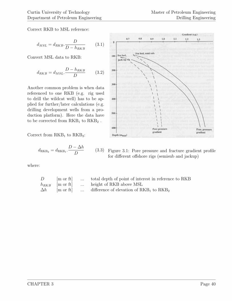
Within drilling, it is common to express pressures as gradients. With this concept, the hydrostaticpressure can be given as equivalent density which is independent of the depth and thus makes itscomprehension and correlations of various concepts easier. On the other hand, when gradientsare applied, it has to be always kept in mind that they are referred to a specific depth. Knowingthis reference depth is essential to compute back the corresponding downhole pressures. Withindrilling engineering, the drilling floor or rotary table (RKB) is the most often used reference depth.Geologists and geophysicists generally prefer to use their data in reference to ground floor or meansea level (MSL).
To correct data expressed in RKB to MSL or do the reverse, following equations can be applied:
CHAPTER 3 Page 39
Curtin University of TechnologyDepartment of Petroleum Engineering
Master of Petroleum EngineeringDrilling Engineering
Figure 3.1: Pore pressure and fracture gradient profilefor different offshore rigs (semisub and jackup)
Correct RKB to MSL reference:
dMSL = dRKB.D
D − hRKB
(3.1)
Convert MSL data to RKB:
dRKB = dMSL.D − hRKB
D(3.2)
Another common problem is when datareferenced to one RKB (e.g. rig usedto drill the wildcat well) has to be ap-plied for further/later calculations (e.g.drilling development wells from a pro-duction platform). Here the data haveto be corrected from RKB1 to RKB2 .
Correct from RKB1 to RKB2:
dRKB2 = dRKB1 .D − ∆h
D(3.3)
where:
D [m or ft] ... total depth of point of interest in reference to RKBhRKB [m or ft] ... height of RKB above MSL∆h [m or ft] ... difference of elevation of RKB1 to RKB2
CHAPTER 3 Page 40
Curtin University of TechnologyDepartment of Petroleum Engineering
Master of Petroleum EngineeringDrilling Engineering
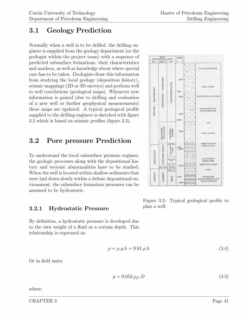
3.1 Geology Prediction
Figure 3.2: Typical geological profile toplan a well
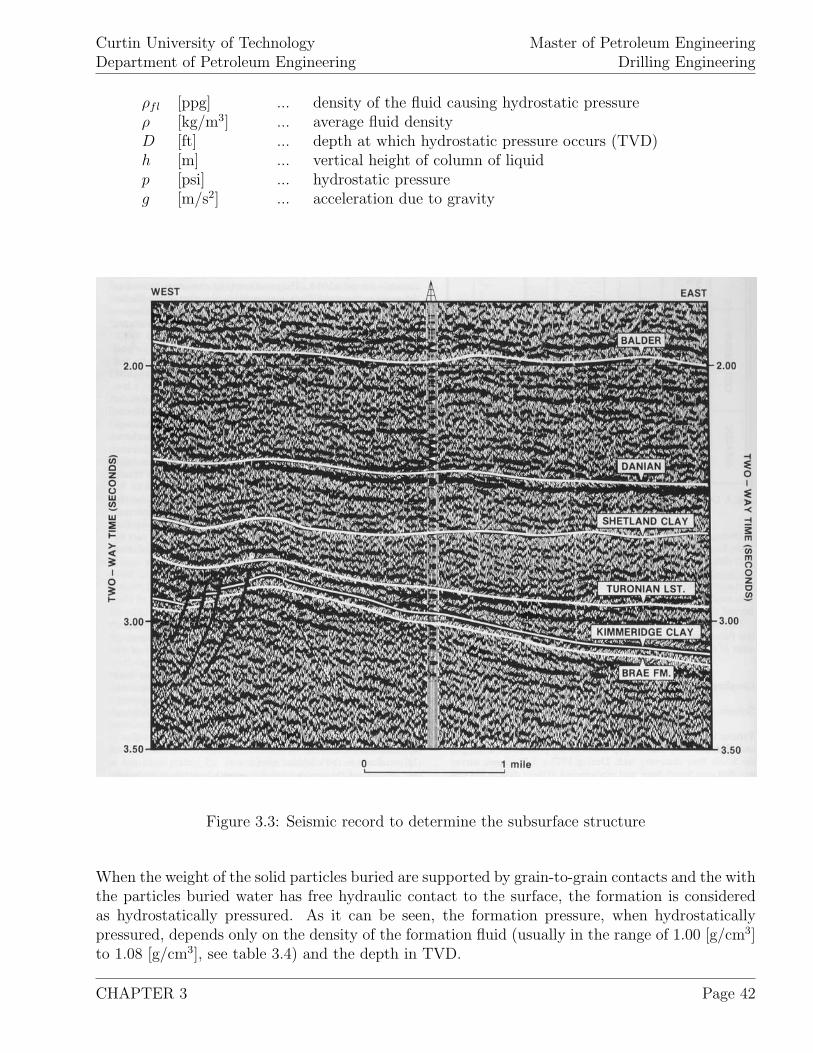
Normally when a well is to be drilled, the drilling en-gineer is supplied from the geology department (or thegeologist within the project team) with a sequence ofpredicted subsurface formations, their characteristicsand markers, as well as knowledge about where specialcare has to be taken. Geologists draw this informationfrom studying the local geology (deposition history),seismic mappings (2D or 3D surveys) and perform wellto well correlations (geological maps). Whenever newinformation is gained (due to drilling and evaluationof a new well or further geophysical measurements)these maps are updated. A typical geological profilesupplied to the drilling engineer is sketched with figure3.2 which is based on seismic profiles (figure 3.3).
3.2 Pore pressure Prediction
To understand the local subsurface pressure regimes,the geologic processes along with the depositional his-tory and tectonic abnormalities have to be studied.When the well is located within shallow sediments thatwere laid down slowly within a deltaic depositional en-vironment, the subsurface formation pressures can beassumed to be hydrostatic.
3.2.1 Hydrostatic Pressure
By definition, a hydrostatic pressure is developed dueto the own weight of a fluid at a certain depth. Thisrelationship is expressed as:
p = ρ.g.h = 9.81.ρ.h (3.4)
Or in field units:
p = 0.052.ρfl.D (3.5)
where:
CHAPTER 3 Page 41
Curtin University of TechnologyDepartment of Petroleum Engineering
Master of Petroleum EngineeringDrilling Engineering
ρfl [ppg] ... density of the fluid causing hydrostatic pressureρ [kg/m3] ... average fluid densityD [ft] ... depth at which hydrostatic pressure occurs (TVD)h [m] ... vertical height of column of liquidp [psi] ... hydrostatic pressureg [m/s2] ... acceleration due to gravity
Figure 3.3: Seismic record to determine the subsurface structure
When the weight of the solid particles buried are supported by grain-to-grain contacts and the withthe particles buried water has free hydraulic contact to the surface, the formation is consideredas hydrostatically pressured. As it can be seen, the formation pressure, when hydrostaticallypressured, depends only on the density of the formation fluid (usually in the range of 1.00 [g/cm3]to 1.08 [g/cm3], see table 3.4) and the depth in TVD.
CHAPTER 3 Page 42
Curtin University of TechnologyDepartment of Petroleum Engineering
Master of Petroleum EngineeringDrilling Engineering
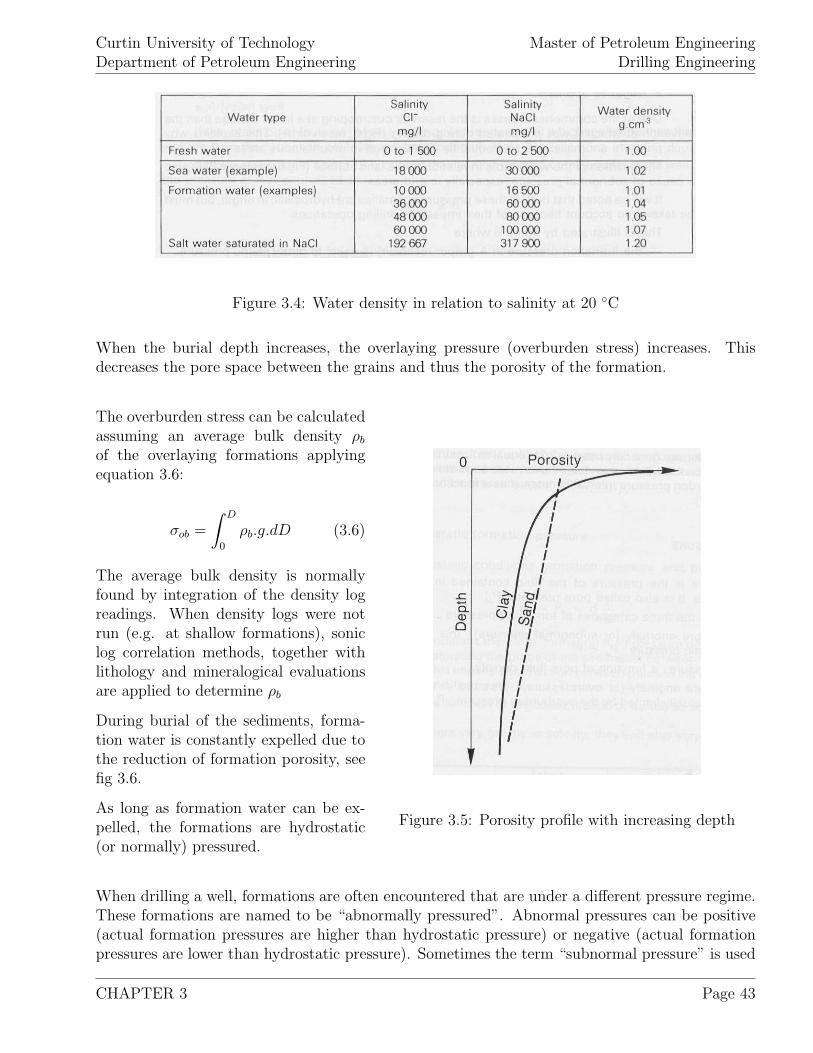
Figure 3.4: Water density in relation to salinity at 20 ◦C
When the burial depth increases, the overlaying pressure (overburden stress) increases. Thisdecreases the pore space between the grains and thus the porosity of the formation.
Figure 3.5: Porosity profile with increasing depth
The overburden stress can be calculatedassuming an average bulk density ρb
of the overlaying formations applyingequation 3.6:
σob =
∫ D
0
ρb.g.dD (3.6)
The average bulk density is normallyfound by integration of the density logreadings. When density logs were notrun (e.g. at shallow formations), soniclog correlation methods, together withlithology and mineralogical evaluationsare applied to determine ρb
During burial of the sediments, forma-tion water is constantly expelled due tothe reduction of formation porosity, seefig 3.6.
As long as formation water can be ex-pelled, the formations are hydrostatic(or normally) pressured.
When drilling a well, formations are often encountered that are under a different pressure regime.These formations are named to be “abnormally pressured”. Abnormal pressures can be positive(actual formation pressures are higher than hydrostatic pressure) or negative (actual formationpressures are lower than hydrostatic pressure). Sometimes the term “subnormal pressure” is used
CHAPTER 3 Page 43
Curtin University of TechnologyDepartment of Petroleum Engineering
Master of Petroleum EngineeringDrilling Engineering
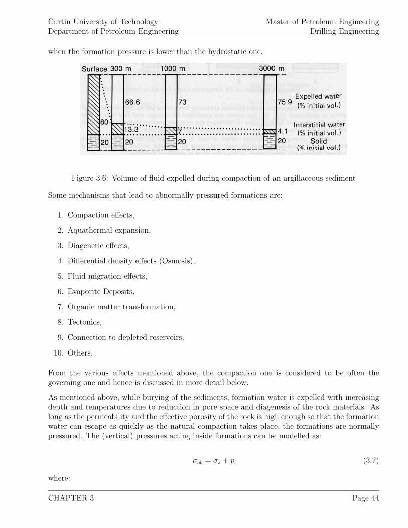
when the formation pressure is lower than the hydrostatic one.
Figure 3.6: Volume of fluid expelled during compaction of an argillaceous sediment
Some mechanisms that lead to abnormally pressured formations are:
1. Compaction effects,
2. Aquathermal expansion,
3. Diagenetic effects,
4. Differential density effects (Osmosis),
5. Fluid migration effects,
6. Evaporite Deposits,
7. Organic matter transformation,
8. Tectonics,
9. Connection to depleted reservoirs,
10. Others.
From the various effects mentioned above, the compaction one is considered to be often thegoverning one and hence is discussed in more detail below.
As mentioned above, while burying of the sediments, formation water is expelled with increasingdepth and temperatures due to reduction in pore space and diagenesis of the rock materials. Aslong as the permeability and the effective porosity of the rock is high enough so that the formationwater can escape as quickly as the natural compaction takes place, the formations are normallypressured. The (vertical) pressures acting inside formations can be modelled as:
σob = σz + p (3.7)
where:
CHAPTER 3 Page 44
Curtin University of TechnologyDepartment of Petroleum Engineering
Master of Petroleum EngineeringDrilling Engineering
σob [psi] ... overburden stressσz [psi] ... vertical stress supported by the grain-to-grain connectionsp [psi] ... formation pore pressure
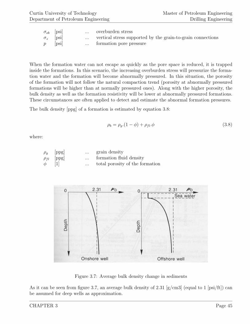
When the formation water can not escape as quickly as the pore space is reduced, it is trappedinside the formations. In this scenario, the increasing overburden stress will pressurize the forma-tion water and the formation will become abnormally pressured. In this situation, the porosityof the formation will not follow the natural compaction trend (porosity at abnormally pressuredformations will be higher than at normally pressured ones). Along with the higher porosity, thebulk density as well as the formation resistivity will be lower at abnormally pressured formations.These circumstances are often applied to detect and estimate the abnormal formation pressures.
The bulk density [ppg] of a formation is estimated by equation 3.8:
ρb = ρg.(1 − φ) + ρfl.φ (3.8)
where:
ρg [ppg] ... grain densityρfl [ppg] ... formation fluid densityφ [1] ... total porosity of the formation
Figure 3.7: Average bulk density change in sediments
As it can be seen from figure 3.7, an average bulk density of 2.31 [g/cm3] (equal to 1 [psi/ft]) canbe assumed for deep wells as approximation.
CHAPTER 3 Page 45
Curtin University of TechnologyDepartment of Petroleum Engineering
Master of Petroleum EngineeringDrilling Engineering
In areas of frequent drilling activities or where formation evaluation is carried out extensively, thenatural trend of bulk density change with depth is known.
For shale formations that follow the natural compaction trend, it has been observed that theporosity change with depth can be described using below relationship:
φ = φo.e−K.Ds (3.9)
where:
φ [1] ... porosity at depth of interestφo [1] ... porosity at the surfaceK [ft−1] ... porosity decline constant, specific for each locationDs [ft] ... depth of interest (TVD)
When equation 3.9 is substituted in equation 3.8 and equation 3.6 and after integration theoverburden stress profile is found for an offshore well as:
σob = 0.052.ρsw.Dw + 0.052.ρg.Dg − 0.052
K.(ρg − ρfl).φo.(1 − e−K.Dg) (3.10)
where:
Dg [ft] ... depth of sediment from sea bottomρsw [ppg] ... sea water density
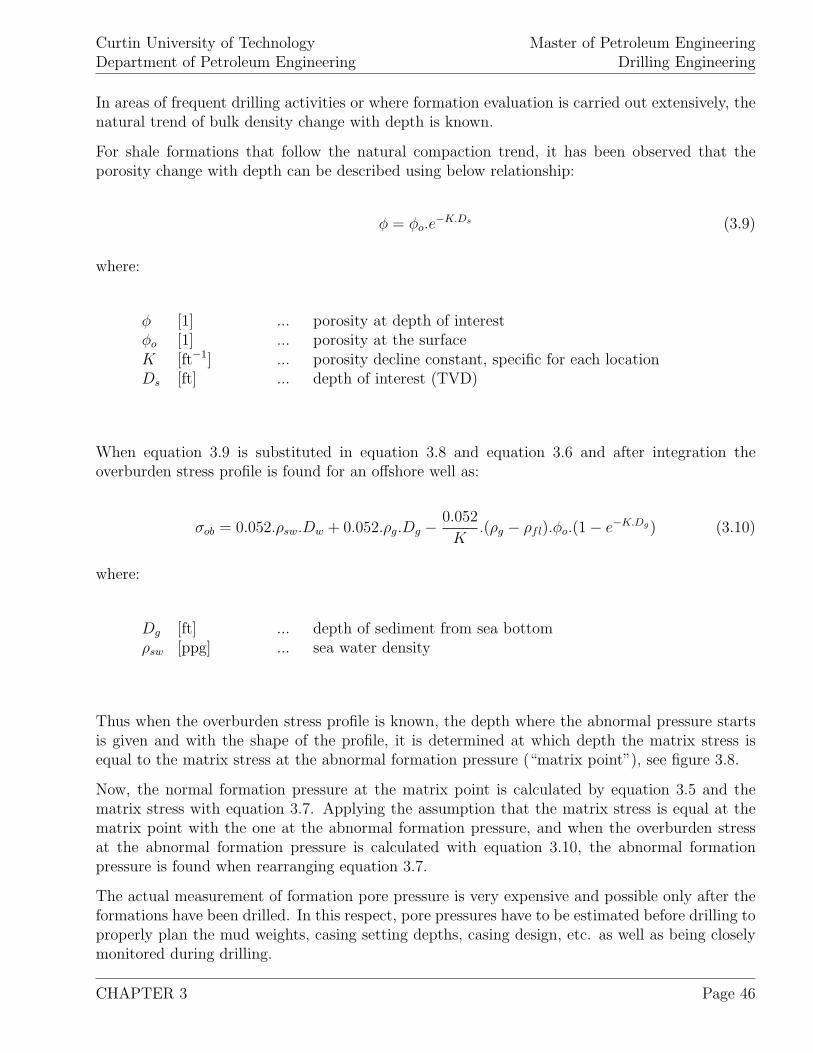
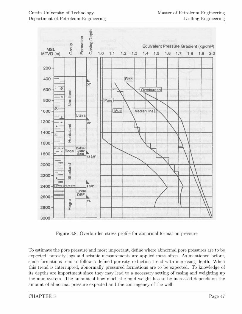
Thus when the overburden stress profile is known, the depth where the abnormal pressure startsis given and with the shape of the profile, it is determined at which depth the matrix stress isequal to the matrix stress at the abnormal formation pressure (“matrix point”), see figure 3.8.
Now, the normal formation pressure at the matrix point is calculated by equation 3.5 and thematrix stress with equation 3.7. Applying the assumption that the matrix stress is equal at thematrix point with the one at the abnormal formation pressure, and when the overburden stressat the abnormal formation pressure is calculated with equation 3.10, the abnormal formationpressure is found when rearranging equation 3.7.
The actual measurement of formation pore pressure is very expensive and possible only after theformations have been drilled. In this respect, pore pressures have to be estimated before drilling toproperly plan the mud weights, casing setting depths, casing design, etc. as well as being closelymonitored during drilling.
CHAPTER 3 Page 46
Curtin University of TechnologyDepartment of Petroleum Engineering
Master of Petroleum EngineeringDrilling Engineering
Figure 3.8: Overburden stress profile for abnormal formation pressure
To estimate the pore pressure and most important, define where abnormal pore pressures are to beexpected, porosity logs and seismic measurements are applied most often. As mentioned before,shale formations tend to follow a defined porosity reduction trend with increasing depth. Whenthis trend is interrupted, abnormally pressured formations are to be expected. To knowledge ofits depths are importment since they may lead to a necessary setting of casing and weighting upthe mud system. The amount of how much the mud weight has to be increased depends on theamount of abnormal pressure expected and the contingency of the well.
CHAPTER 3 Page 47
Curtin University of TechnologyDepartment of Petroleum Engineering
Master of Petroleum EngineeringDrilling Engineering
Abnormal pressure detection while drilling
When the well is in progress and abnormal formation pressures are expected, various parametersare observed and cross-plotted. Some of these while drilling detection methods are:
(a) Penetration rate,(b) “d” exponent,(c) Sigmalog,(d) Various drilling rate normalisations,(e) Torque measurements,(f) Overpull and drag,(g) Hole fill,(h) Pit level – differential flow – pump pressure,(i) Measurements while drilling,(j) Mud gas,(k) Mud density,(l) Mud temperature,(m) Mud resistivity,(n) Lithology,(o) Shale density,(p) Shale factor (CEC),(q) Shape, size and abundance of cuttings,(r) Cuttings gas,(s) X-ray diffraction,(t) Oil show analyzer,(u) Nuclear magnetic resonance.
d-exponent
It has been observed that when the same formation is drilled applying the same drilling parameters(WOB, RPM, hydraulics, etc.), a change in rate of penetration is caused by the change of differ-ential pressure (borehole pressure - formation pressure). Here an increase of differential pressure(a decrease of formation pressure) causes a decrease of ROP, a decrease of differential pressure (in-crease of formation pressure) an increase of ROP. Applying this observation to abnormal formationpressure detection, the so called “d-exponent” was developed.
d =log10
R60.N
log1012.W106.D
(3.11)
where:
R [ft/hr] ... penetration rateN [rev./min] ... rotation speed
CHAPTER 3 Page 48
Curtin University of TechnologyDepartment of Petroleum Engineering
Master of Petroleum EngineeringDrilling Engineering
W [lb] ... weight on bitD [in] ... hole seize
The term R60.N
is always less than 1 and represents penetration in feet per drilling table rotation.
Wile drilling is in progress, a d-exponent log is been drawn. Any decrease of the d-exponent valuein an argillaceous sequence is commonly interpreted with the respective degree of undercompactionand associated with abnormal pressure. Practice has shown that the d-exponent is not sufficient toconclude for abnormal pressured formations. The equation determining the d-exponent assumesa constant mud weight. In practice, mud weight is changed during the well proceeds. Since achange in mud weight results in a change of d-exponent, a new trend line for each mud weight hasto be established, which needs the drilling of a few tenth of feet. To account for this effect, the socalled “corrected d-exponent” dc was developed:
dc = d.ρfl
ρeqv
(3.12)
where:
d ... d-exponent calculated with equation 3.11ρfl [ppg] ... formation fluid density for the hydrostatic gradient in the regionρeqv [ppg] ... mud weight
Abnormal pressure evaluation
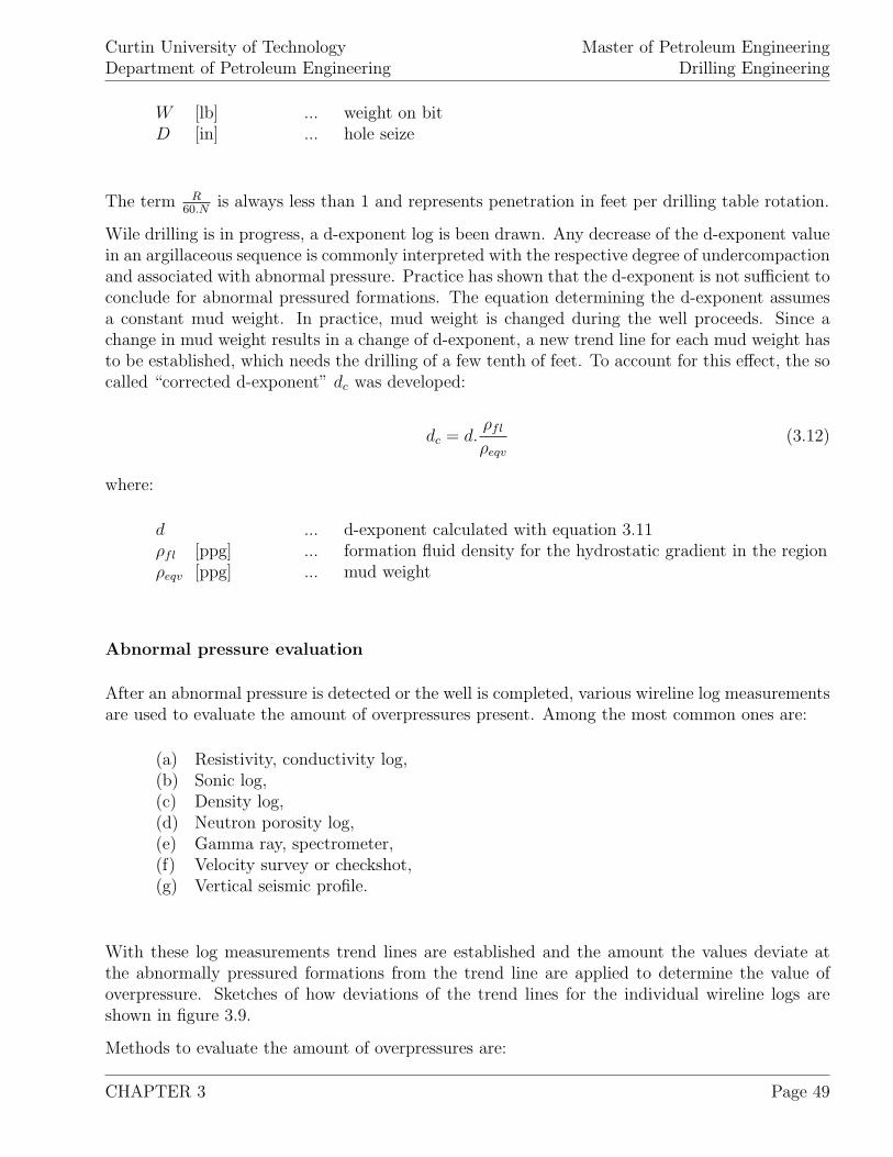
After an abnormal pressure is detected or the well is completed, various wireline log measurementsare used to evaluate the amount of overpressures present. Among the most common ones are:
(a) Resistivity, conductivity log,(b) Sonic log,(c) Density log,(d) Neutron porosity log,(e) Gamma ray, spectrometer,(f) Velocity survey or checkshot,(g) Vertical seismic profile.
With these log measurements trend lines are established and the amount the values deviate atthe abnormally pressured formations from the trend line are applied to determine the value ofoverpressure. Sketches of how deviations of the trend lines for the individual wireline logs areshown in figure 3.9.
Methods to evaluate the amount of overpressures are:
CHAPTER 3 Page 49
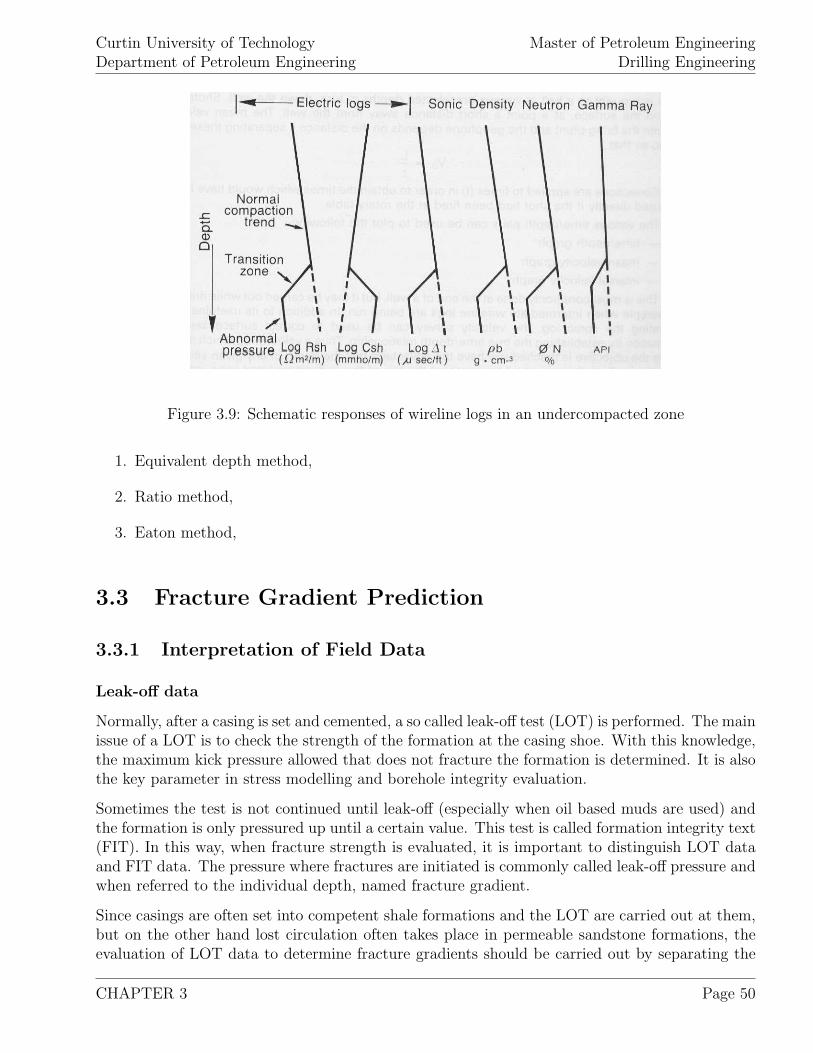
Curtin University of TechnologyDepartment of Petroleum Engineering
Master of Petroleum EngineeringDrilling Engineering
Figure 3.9: Schematic responses of wireline logs in an undercompacted zone
1. Equivalent depth method,
2. Ratio method,
3. Eaton method,
3.3 Fracture Gradient Prediction
3.3.1 Interpretation of Field Data
Leak-off data
Normally, after a casing is set and cemented, a so called leak-off test (LOT) is performed. The mainissue of a LOT is to check the strength of the formation at the casing shoe. With this knowledge,the maximum kick pressure allowed that does not fracture the formation is determined. It is alsothe key parameter in stress modelling and borehole integrity evaluation.
Sometimes the test is not continued until leak-off (especially when oil based muds are used) andthe formation is only pressured up until a certain value. This test is called formation integrity text(FIT). In this way, when fracture strength is evaluated, it is important to distinguish LOT dataand FIT data. The pressure where fractures are initiated is commonly called leak-off pressure andwhen referred to the individual depth, named fracture gradient.
Since casings are often set into competent shale formations and the LOT are carried out at them,but on the other hand lost circulation often takes place in permeable sandstone formations, theevaluation of LOT data to determine fracture gradients should be carried out by separating the
CHAPTER 3 Page 50
Curtin University of TechnologyDepartment of Petroleum Engineering
Master of Petroleum EngineeringDrilling Engineering
data into two groups, one concerning the competent shale formations with higher fracture gradientsand a second one for permeable sandstone (coal, chalk, etc.) formations exhibiting weaker fracturegradients.
When LOT data are evaluated, a considerable spread is often found. It is common practice tofirst plot the LOT values vs. depth and check how well they correlate. When the spread of LOTvalues is to large to define a correlation line, the “effective stress concept” can be applied.
Effective stresses
The effective stress concept states that the stress in the rock matrix is equal the total stress minusthe pore pressure. This is expressed in equation 3.13:
σeff = σt − Po (3.13)
Horizontal stresses
When the borehole is vertical, as well as a hydrostatic stress state is assumed, the LOT valuescan be expressed as:
LOT = 2.σa − Po (3.14)
where:
LOT [psi] ... leak-off test valueσa [psi] ... average horizontal stressPo [psi] ... pore pressure
Since when the LOT is carried out, the pore pressure is known or measured as well, the horizontalstress can be evaluated by equation 3.15:
σa =LOT − Po
2(3.15)
The horizontal stress as derived above can also be used for a correlation when plotted vs. depth.
Influence of hole inclination
Since formations are generally not isotropic or even under a hydrostatic stress state which wasassumed above, fracture gradients do normally depend on the inclination of the borehole. Toaccount for this, the coupling of the fracture gradient of an inclined hole with a vertical one canbe modeled by equation 3.16:
CHAPTER 3 Page 51
Curtin University of TechnologyDepartment of Petroleum Engineering
Master of Petroleum EngineeringDrilling Engineering
Pwf (θ) = Pwf (0) +1
3.(Po − P ∗
o ). sin2 θ (3.16)
where:
Pwf (θ) [psi] ... fracture gradient at α inclined boreholePwf (0) [psi] ... fracture gradient at vertical boreholePo [psi] ... pore pressure at specific depthP ∗
o [psi] ... pore pressure constantθ [rad] ... borehole inclination
Fracture gradients at shallow depth
The determination of fracture gradients for shallow depth is often difficult since very little dataexists. This is due to the circumstance that at shallow depth, blowout preventers are oftennot installed and thus no pressure testing can be carried out. Especially at offshore wells, theknowledge of shallow fracture gradients are important since the margin between pore pressure andfracture gradient is narrow and the danger of shallow gas pockets exists. As practice shows, thespread of fracture gradients are larger at shallow depths and decrease with depth.
3.4 Mud Weight Planning
Selecting the correct mud weight for drilling the individual sections comprises a key factor torealize a in-gauge hole and avoid various borehole problems.
Too low mud weight may result in collapse and fill problems (well cleaning), while too high mudweight may result in mud losses or pipe sticking. Practice has also shown that excessive variationsin mud weight may lead to borehole failure (fatigue type effect), thus a more constant mud weightprogram should be aimed for. Along with a more constant mud weight program, the equivalentcirculation density (ECD) as well as the surge and swab pressures shall be kept within limits.
Washouts of the borehole are sometimes caused by jet actions of the bit nozzles but also sometimesby to low mud weight causing a breakdown of the borehole wall. A higher mud weight will thereforebalance the rock stresses better and tend to keep the borehole more in-gauge.
A decease in hole diameter is often due to swelling (clay swelling) requiring wiper trips or back-reaming. This necessity is sometimes reduced by higher mud weights.
An increased mud weight increases the danger of becoming differential stuck at permeable for-mations. Therefore mud weight shall not be chosen to be to high. However, what is sometimesbelieved to be a differentially stuck drillstring is sometimes due to a borehole collapse which packsthe hole around the bottom-hole assembly. A lower mud weight also causes breakouts of shalelayers leaving sand formations in-gauge, see figure 3.10. This can increase the danger of gettingdifferential stuck at the exposed sand stringers.
CHAPTER 3 Page 52
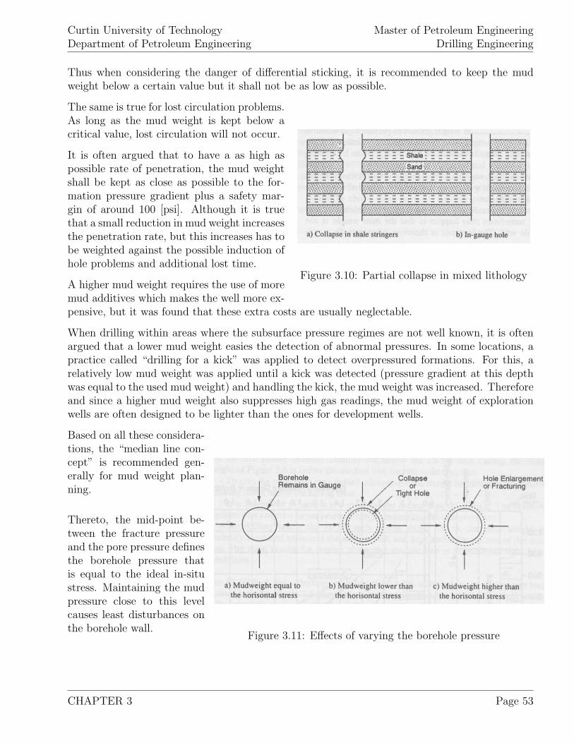
Curtin University of TechnologyDepartment of Petroleum Engineering
Master of Petroleum EngineeringDrilling Engineering
Thus when considering the danger of differential sticking, it is recommended to keep the mudweight below a certain value but it shall not be as low as possible.
Figure 3.10: Partial collapse in mixed lithology
The same is true for lost circulation problems.As long as the mud weight is kept below acritical value, lost circulation will not occur.
It is often argued that to have a as high aspossible rate of penetration, the mud weightshall be kept as close as possible to the for-mation pressure gradient plus a safety mar-gin of around 100 [psi]. Although it is truethat a small reduction in mud weight increasesthe penetration rate, but this increases has tobe weighted against the possible induction ofhole problems and additional lost time.
A higher mud weight requires the use of moremud additives which makes the well more ex-pensive, but it was found that these extra costs are usually neglectable.
When drilling within areas where the subsurface pressure regimes are not well known, it is oftenargued that a lower mud weight easies the detection of abnormal pressures. In some locations, apractice called “drilling for a kick” was applied to detect overpressured formations. For this, arelatively low mud weight was applied until a kick was detected (pressure gradient at this depthwas equal to the used mud weight) and handling the kick, the mud weight was increased. Thereforeand since a higher mud weight also suppresses high gas readings, the mud weight of explorationwells are often designed to be lighter than the ones for development wells.
Figure 3.11: Effects of varying the borehole pressure
Based on all these considera-tions, the “median line con-cept” is recommended gen-erally for mud weight plan-ning.
Thereto, the mid-point be-tween the fracture pressureand the pore pressure definesthe borehole pressure thatis equal to the ideal in-situstress. Maintaining the mudpressure close to this levelcauses least disturbances onthe borehole wall.
CHAPTER 3 Page 53
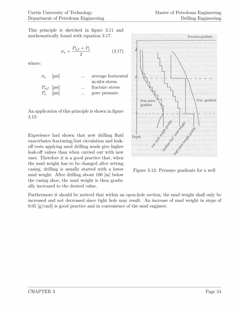
Curtin University of TechnologyDepartment of Petroleum Engineering
Master of Petroleum EngineeringDrilling Engineering
Figure 3.12: Pressure gradients for a well
This principle is sketched in figure 3.11 andmathematically found with equation 3.17:
σa =Pwf + Po
2(3.17)
where:
σa [psi] ... average horizontalin-situ stress
Pwf [psi] ... fracture stressPo [psi] ... pore pressure
An application of this principle is shown in figure3.12:
Experience had shown that new drilling fluidexacerbates fracturing/lost circulation and leak-off tests applying used drilling muds give higherleak-off values than when carried out with newones. Therefore it is a good practice that, whenthe mud weight has to be changed after settingcasing, drilling is usually started with a lowermud weight. After drilling about 100 [m] belowthe casing shoe, the mud weight is then gradu-ally increased to the desired value.
Furthermore it should be noticed that within an open-hole section, the mud weight shall only beincreased and not decreased since tight hole may result. An increase of mud weight in steps of0.05 [g/cm3] is good practice and in convenience of the mud engineer.
CHAPTER 3 Page 54

Curtin University of TechnologyDepartment of Petroleum Engineering
Master of Petroleum EngineeringDrilling Engineering
3.5 Examples
CHAPTER 3 Page 55

Curtin University of TechnologyDepartment of Petroleum Engineering
Master of Petroleum EngineeringDrilling Engineering
CHAPTER 3 Page 56
Curtin University of TechnologyDepartment of Petroleum Engineering
Master of Petroleum EngineeringDrilling Engineering
Chapter 4
Drilling Hydraulics
To realize a safe, efficient and cost-effective drilling project, drilling hydraulics, also known as righydraulics, play an important role. The different aspects that make up optimum rig hydraulicsare:
1. Hydraulic energy impact on the bit,
2. Friction pressure losses through the surface equipment, drillstring, annuli and drill bit,
3. Efficient hole cleaning,
4. Nozzle selection and,
5. Produced pump pressure.
Some of the drilling problems that are due to improperly designed drilling hydraulics are failure ofsufficient hole cleaning leaving cuttings in the hole and lead to stuck pipe, lost circulation causingkicks and slow penetration rates.
To understand the various dependencies of efficient drilling hydraulics, the hydrostatic pressureinside the wellbore, types of fluid flow, criteria of fluid flow and commonly used fluid types fordifferent drilling operations are discussed. By understanding these concepts various aspects of thedesign of the hydraulics system like
1. Pressure losses (surface equipment, drillstring, bit, annulus),
2. Bit nozzle seize selection,
3. Surge and swab pressure due to drillstring movement,
4. Optimization of bit hydraulics,
5. Carrying capacity of the drilling fluid.
are discussed further on.
CHAPTER 4 Page 57
Curtin University of TechnologyDepartment of Petroleum Engineering
Master of Petroleum EngineeringDrilling Engineering
4.1 Hydrostatic Pressure Inside the Wellbore
For oil well applications, the fluid may be mud, foam, mist, air or natural gas. For a complex fluidcolumn consisting of multiple fluids, the hydrostatic pressure is given in field units by:
p = 0.052.n∑
i=1
ρm. (Di − Di−1) (4.1)
where:
ρmi [ppg] ... mud weight of the ith fluid column
When gas is present in the well, the hydrostatic pressure developed by the gas column is calculatedwith:
p = po.e
M.(D−Do)
1,544.z.(Tf +460) (4.2)
where:
z [1] ... real gas deviation factorpo [psi] ... surface pressureD [ft] ... total depth (TVD)Tf [F] ... bottom hole temperature of the formation
The molecular weight M of the gas is found as:
M =80.3.z. (T + 460) .ρg
p(4.3)
where:
ρg [ppg] ... density of the gasT [F] ... average gas density
For practical purposes, the hydrostatics due to a complex fluid column are converted to an equiva-lent single-fluid hydrostatic pressure. To do this, all individual hydrostatic pressures are summed
CHAPTER 4 Page 58
Curtin University of TechnologyDepartment of Petroleum Engineering
Master of Petroleum EngineeringDrilling Engineering
up for a specific depth pd and then converted to an equivalent mud weight ρe [ppg] that wouldcause the same hydrostatic pressure.
ρe =pd
0.052.D(4.4)
Therefore the equivalent mud weight has to be always referenced to a specific depth.
As the mud is used to transport the cuttings from the bottom of the hole to the surface andpenetrated formations often contain a certain amount of formation gas, the mud column at theannulus is usually mixed with solids and gas. This alters the weight of the mud at the annulus.The new average mud weight ρm of a mixture containing mud and solids can be calculated as:
ρm =
∑ni=1 mi∑ni=1 Vi
=
∑ni+1 ρi.Vi∑n
i=1 Vi
=n∑
i=1
ρi.fi (4.5)
where:
mi [lbm] ... mass of component iVi [gal] ... volume of component iρi [ppg] ... density of component ifi [1] ... volume fraction of component i
I should be noted that only solids that are suspended within the mud do alter the mud weight.Settled particles do not affect the hydrostatic pressure.
If gas is present in the mud column as well, the density of the gas component is a function of thedepth and will decrease with decreasing pressure. In this way, the density of mud containing gasis decreasing with decreasing depth.
When the gas-liquid mixture is highly pressured (e.g. deep section of the well), the variation ofthe gas density can be ignored and the average mud density containing gas calculated with:
ρ = ρf .(1 − fg) + ρg.fg =(ρf + M.Nν) .p
p + z.Nν .R.T(4.6)
where:
fg =z.Nν .
R.Tp
1 + z.Nν .R.T
p
(4.7)
CHAPTER 4 Page 59
Curtin University of TechnologyDepartment of Petroleum Engineering
Master of Petroleum EngineeringDrilling Engineering
fg [1] ... volume fraction of gasρg [ppg] ... density of gasNν [# moles] ... moles of gas dispersed in one gallon of mud
When the variation of gas density can not be ignored (e.g. shallow depth), the equation 4.8 hasto be solved by iteration to compute the change in pressure:
D2 − D1 =p2 − p1
0.052. (ρf + M.Nν)+
z.Nν .R.T
0.052. (ρf + M.Nν). ln
p2
p1
(4.8)
where:
z is calculated at p = p2+p1
2
It is essential to understand that well control and the safety of drilling operations are stronglydepended on the maintenance of proper hydrostatic pressure. This pressure is needed to counter-balance the formation pressure. In case the hydrostatic pressure in the borehole is higher than theformation pressure, the situation is called “over-balanced”. This prevents kicks (fluid flow from theformation into the borehole) and causes at permeable formations an intrusion of some mud (watercomponent) into the formation. The intrusion is stopped by the built up of mud cake that sealsoff permeable formations. On the other hand, the hydrostatic pressure inside the borehole mustnot be higher than the fracture pressure of the formations penetrated since this would fracturethe formation artificially, cause loss of circulation and lead to well control problems. To obtainmaximum penetration rates the hydrostatic pressure should be kept as close as practical to theformation pressure since a higher differential pressure (hydrostatic pressure - formation pressure)leads to worst cutting removal from the bottom of the well. Due to this circumstance, underbal-anced drilling techniques have been developed that use air, foam or mist as drilling fluids. Herethe formation pressure is higher than the hydrostatic pressure caused by the mud and thus thewell is constantly kicking. With underbalanced drilling techniques much higher penetration ratesare possible but well control can be a problem. Therefore underbalanced drilling is prohibited bysome governments and/or in some areas.
4.2 Types of Fluid Flow
Since multiple aspects of drilling and completion operations require the understanding of how fluidmoves through pipes, fittings and annulus, the knowledge of basic fluid flow patterns is essential.Generally, fluid movement can be described as laminar, turbulent or in transition between laminarand turbulent.
It should be understood that rotation and vibrations influence the rheological properties of drillingfluids. Also the pulsing of the mud pumps cause variations in the flow rates as well as the meanflow rates. Furthermore changing solid content influences the actual mud density and its plasticviscosity.
CHAPTER 4 Page 60
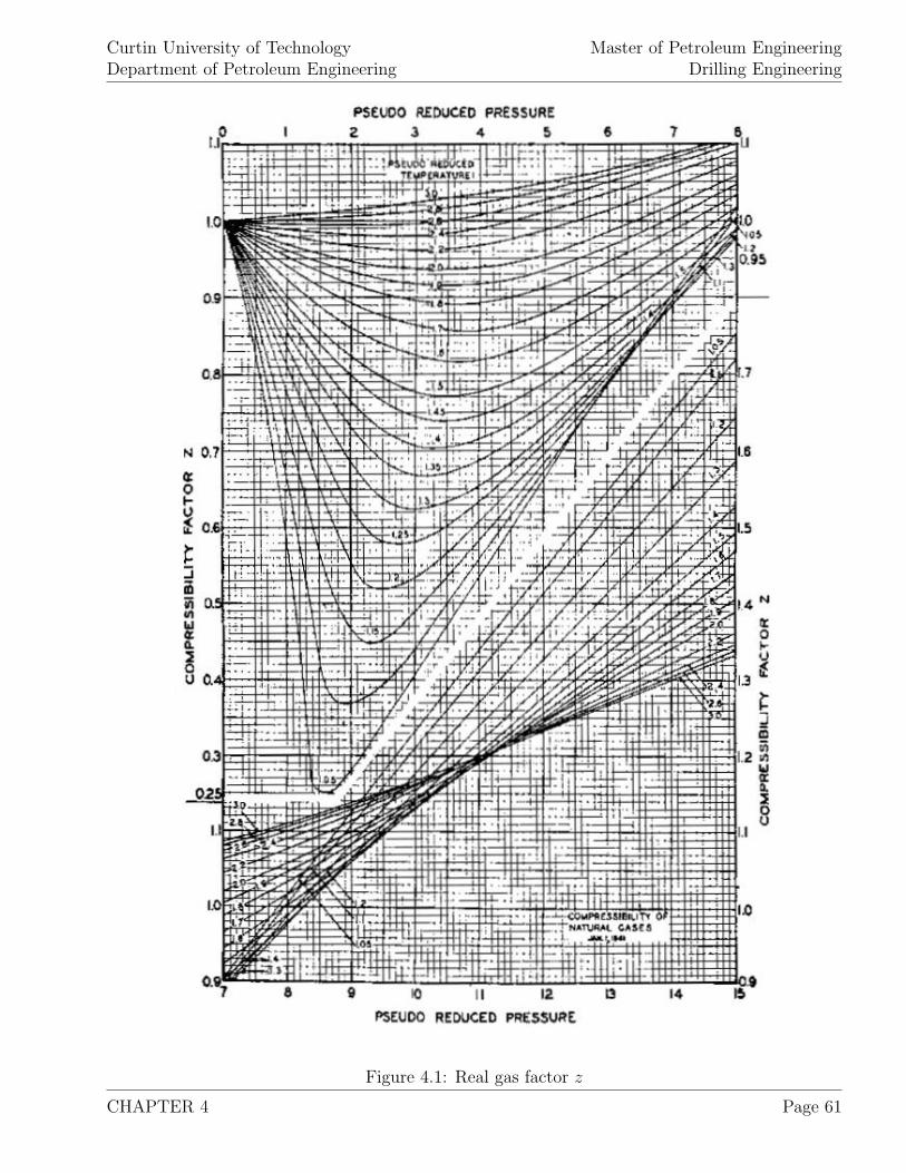
Curtin University of TechnologyDepartment of Petroleum Engineering
Master of Petroleum EngineeringDrilling Engineering
Figure 4.1: Real gas factor z
CHAPTER 4 Page 61
Curtin University of TechnologyDepartment of Petroleum Engineering
Master of Petroleum EngineeringDrilling Engineering
Fluid movement, when laminar flow is present, can be described as in layers or “laminae”. Here atall times the direction of fluid particle movement is parallel to each other and along the directionof flow. In this way no mixture or interchange of fluid particles from one layer to another takesplace. At turbulent flow behavior, which develops at higher average flow velocities, secondaryirregularities such as vortices and eddys are imposed to the flow. This causes a chaotic particlemovement and thus no orderly shear between fluid layers is present.
The so called “Reynolds number” is often used to distinguish the different flow patterns. Af-ter defining the current flow pattern, different equations are applied to calculate the respectivepressure drops.
For the flow through pipes, the Reynolds number is determined with:
NRe =928.ρm.ν.di
µ(4.9)
ν =q, [gal/min]
2.448.d2i
=17.16. (q, [bbl/min])
d2i
(4.10)
and for the flow through annuli:
NRe =928.ρm.ν.de
µ(4.11)
ν =q, [gal/min]
2.448. (d22 − d2
1)=
17.16. (q, [bbl/min])
d22 − d2
1
(4.12)
de = 0.816. (d2 − d1) (4.13)
where:
ρ [ppg] ... fluid densitydi [in] ... inside pipe diameterν [ft/sec] ... mean fluid velocityµ [cp] ... fluid viscosityde [in] ... equivalent diameter of annulusd2 [in] ... internal diameter of outer pipe or boreholed1 [in] ... external diameter of inner pipe
The different flow patterns are then characterised considering the Reynolds number. Normallythe Reynolds number 2,320 distinguishes the laminar and turbulent flow behavior, for drillingpurposes a value of 2,000 is applied instead. Furthermore it is assumed that turbulent flow is fully
CHAPTER 4 Page 62
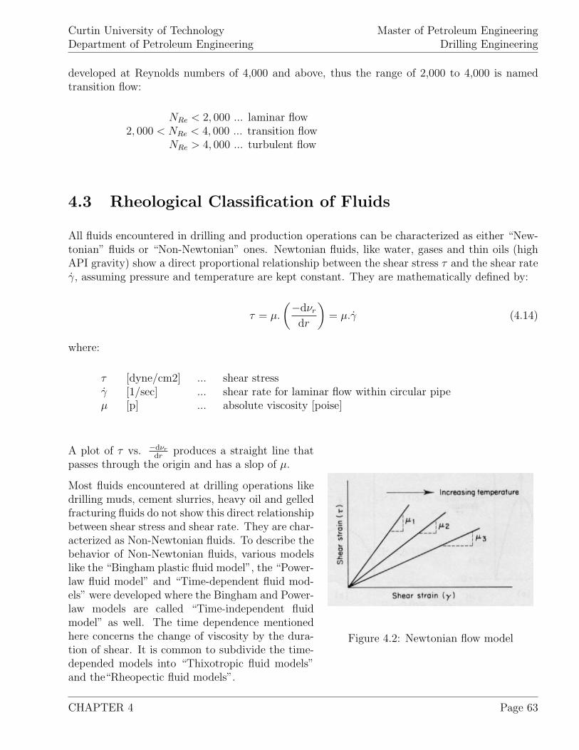
Curtin University of TechnologyDepartment of Petroleum Engineering
Master of Petroleum EngineeringDrilling Engineering
developed at Reynolds numbers of 4,000 and above, thus the range of 2,000 to 4,000 is namedtransition flow:
NRe < 2, 000 ... laminar flow2, 000 < NRe < 4, 000 ... transition flow
NRe > 4, 000 ... turbulent flow
4.3 Rheological Classification of Fluids
All fluids encountered in drilling and production operations can be characterized as either “New-tonian” fluids or “Non-Newtonian” ones. Newtonian fluids, like water, gases and thin oils (highAPI gravity) show a direct proportional relationship between the shear stress τ and the shear rateγ̇, assuming pressure and temperature are kept constant. They are mathematically defined by:
τ = µ.
(−dνr
dr
)= µ.γ̇ (4.14)
where:
τ [dyne/cm2] ... shear stressγ̇ [1/sec] ... shear rate for laminar flow within circular pipeµ [p] ... absolute viscosity [poise]
Figure 4.2: Newtonian flow model
A plot of τ vs. −dνr
drproduces a straight line that
passes through the origin and has a slop of µ.
Most fluids encountered at drilling operations likedrilling muds, cement slurries, heavy oil and gelledfracturing fluids do not show this direct relationshipbetween shear stress and shear rate. They are char-acterized as Non-Newtonian fluids. To describe thebehavior of Non-Newtonian fluids, various modelslike the “Bingham plastic fluid model”, the “Power-law fluid model” and “Time-dependent fluid mod-els” were developed where the Bingham and Power-law models are called “Time-independent fluidmodel” as well. The time dependence mentionedhere concerns the change of viscosity by the dura-tion of shear. It is common to subdivide the time-depended models into “Thixotropic fluid models”and the“Rheopectic fluid models”.
CHAPTER 4 Page 63

Curtin University of TechnologyDepartment of Petroleum Engineering
Master of Petroleum EngineeringDrilling Engineering
Figure 4.3: Sketch of Bingham fluid model
It shall be understood that all the models men-tioned above are based on different assumptionsthat are hardly valid for all drilling operations, thusthey are valid to a certain extend only.
The Bingham and Power-law fluid models are de-scribed mathematically by:
Bingham plastic fluid model:
τ = τy + µp
(−dνr
dr
)= τy + µp.γ̇ (4.15)
Power-law fluid model:
τ = K.
(−dνr
dr
)n
= K.γ̇n (4.16)
Figure 4.4: Sketch of Power-law fluid model
where:
τy [lbf/100 ft2] ... yield pointµp [cp] ... plastic viscosityn [1] ... flow behavior indexK [1] ... consistency index.
A plot of shear stress vs. shear rate for the Binghammodel will result in a straight line, see sketch 4.3.In contrary to Newtonian fluids, Bingham fluids dohave a yield point τy and it takes a defined shearstress (τt) to initiate flow. Above τy, τ and γ areproportional defined by the viscosity, re-named toplastic viscosity µp
The characteristics of the Power-law fluid model issketched in 4.4. This plot is done on a log-log scaleand results in a straight line. Here the slope deter-mines the flow behavior index n and the interceptwith the vertical, the value of the consistency index(logK).
The flow behavior index, that ranges from 0 to1.0 declares the degree of Non-Newtonian behav-
CHAPTER 4 Page 64

Curtin University of TechnologyDepartment of Petroleum Engineering
Master of Petroleum EngineeringDrilling Engineering
ior, where n = 1.0 indicates a Newtonian fluid. The consistency index K on the other hand givesthe thickness (viscosity) of the fluid where, the larger K, the thicker (more viscous) the fluid is.
Figure 4.5: Viscometer
To determine the rheological properties of a par-ticular fluid, a rotational viscometer with six stan-dard speeds and variable speed settings is used com-monly. In field applications, out of these speeds justtwo are normally used (300 and 600 [rpm]) sincethey are sufficient to determine the required prop-erties.
Following equations are applied to define the pa-rameters of the individual fluid:
Newtonian fluid model:
µa =300
N.θN (4.17)
γ̇ =5.066
r2.N (4.18)
Bingham plastic fluid model:
µp = θ600 − θ300 =300
N2 − N1
. (θN2 − θN1) (4.19)
γ̇ =5.066
r2.N +
479.τy
µp
.
(3.174
r2− 1
)(4.20)
τy = θ300 − µp = θN1 − µp.N1
300(4.21)
τgel = θmax at N = 3 rpm (4.22)
Power-law fluid model:
n = 3.322. log
(θ600
θ300
)=
log(
θN2
θN1
)log(
N2
N1
) (4.23)
CHAPTER 4 Page 65
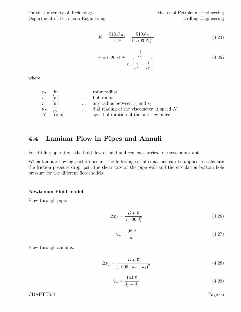
Curtin University of TechnologyDepartment of Petroleum Engineering
Master of Petroleum EngineeringDrilling Engineering
K =510.θ300
511n=
510.θN
(1.703.N)n(4.24)
γ̇ = 0.2094.N.
1
r2n
n.
[1
r2n1
− 1
r2n2
] (4.25)
where:
r2 [in] ... rotor radiusr1 [in] ... bob radiusr [in] ... any radius between r1 and r2
θN [1] ... dial reading of the viscometer at speed NN [rpm] ... speed of rotation of the outer cylinder
4.4 Laminar Flow in Pipes and Annuli
For drilling operations the fluid flow of mud and cement slurries are most important.
When laminar flowing pattern occurs, the following set of equations can be applied to calculatethe friction pressure drop [psi], the shear rate at the pipe wall and the circulation bottom holepressure for the different flow models:
Newtonian Fluid model:
Flow through pipe:
∆pf =D.µ.ν
1, 500.d2i
(4.26)
γ̇w =96.ν
di
(4.27)
Flow through annulus:
∆pf =D.µ.ν
1, 000. (d2 − d1)2 (4.28)
γ̇w =144.ν
d2 − d1
(4.29)
CHAPTER 4 Page 66
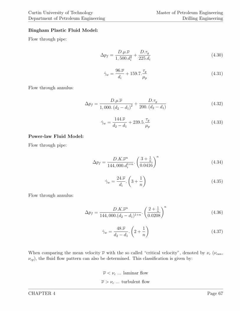
Curtin University of TechnologyDepartment of Petroleum Engineering
Master of Petroleum EngineeringDrilling Engineering
Bingham Plastic Fluid Model:
Flow through pipe:
∆pf =D.µ.ν
1, 500.d2i
+D.τy
225.di
(4.30)
γ̇w =96.ν
di
+ 159.7.τy
µp
(4.31)
Flow through annulus:
∆pf =D.µ.ν
1, 000. (d2 − d1)2 +
D.τy
200. (d2 − d1)(4.32)
γ̇w =144.ν
d2 − d1
+ 239.5.τy
µp
(4.33)
Power-law Fluid Model:
Flow through pipe:
∆pf =D.K.νn
144, 000.d1+ni
.
(3 + 1
n
0.0416
)n
(4.34)
γ̇w =24.ν
di
.
(3 +
1
n
)(4.35)
Flow through annulus:
∆pf =D.K.νn
144, 000.(d2 − d1)1+n.
(2 + 1
n
0.0208
)n
(4.36)
γ̇w =48.ν
d2 − d1
.
(2 +
1
n
)(4.37)
When comparing the mean velocity ν with the so called “critical velocity”, denoted by νc (νcan,νcp), the fluid flow pattern can also be determined. This classification is given by:
ν < νc ... laminar flow
ν > νc ... turbulent flow
CHAPTER 4 Page 67
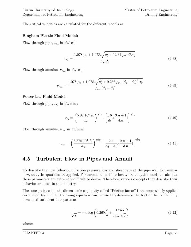
Curtin University of TechnologyDepartment of Petroleum Engineering
Master of Petroleum EngineeringDrilling Engineering
The critical velocities are calculated for the different models as:
Bingham Plastic Fluid Model:
Flow through pipe, νcp in [ft/sec]:
νcp =1.078.µp + 1.078.
õ2
p + 12.34.ρm.d2i .τy
ρm.di
(4.38)
Flow through annulus, νcan in [ft/sec]:
νcan =1.078.µp + 1.078.
õ2
p + 9.256.ρm. (d2 − d1)2 .τy
ρm. (d2 − d1)(4.39)
Power-law Fluid Model:
Flow through pipe, νcp in [ft/min]:
νcp =
(5.82.104.K
ρm
) 12−n
.
[1.6
di
.(3.n + 1
4.n)
] n2−n
(4.40)
Flow through annulus, νcan in [ft/min]:
νcan =
(3.878.104.K
ρm
) 12−n
.
[2.4
d2 − d1
.(2.n + 1
3.n)
] n2−n
(4.41)
4.5 Turbulent Flow in Pipes and Annuli
To describe the flow behaviour, friction pressure loss and shear rate at the pipe wall for laminarflow, analytic equations are applied. For turbulent fluid flow behavior, analytic models to calculatethese parameters are extremely difficult to derive. Therefore, various concepts that describe theirbehavior are used in the industry.
The concept based on the dimensionless quantity called “Friction factor” is the most widely appliedcorrelation technique. Following equation can be used to determine the friction factor for fullydeveloped turbulent flow pattern:
1√f
= −4. log
(0.269.
ε
d+
1.255
NRe.√
f
)(4.42)
where:
CHAPTER 4 Page 68
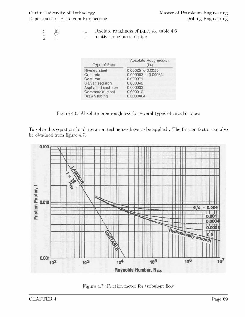
Curtin University of TechnologyDepartment of Petroleum Engineering
Master of Petroleum EngineeringDrilling Engineering
ε [in] ... absolute roughness of pipe, see table 4.6εd
[1] ... relative roughness of pipe
Figure 4.6: Absolute pipe roughness for several types of circular pipes
To solve this equation for f , iteration techniques have to be applied . The friction factor can alsobe obtained from figure 4.7.
Figure 4.7: Friction factor for turbulent flow
CHAPTER 4 Page 69
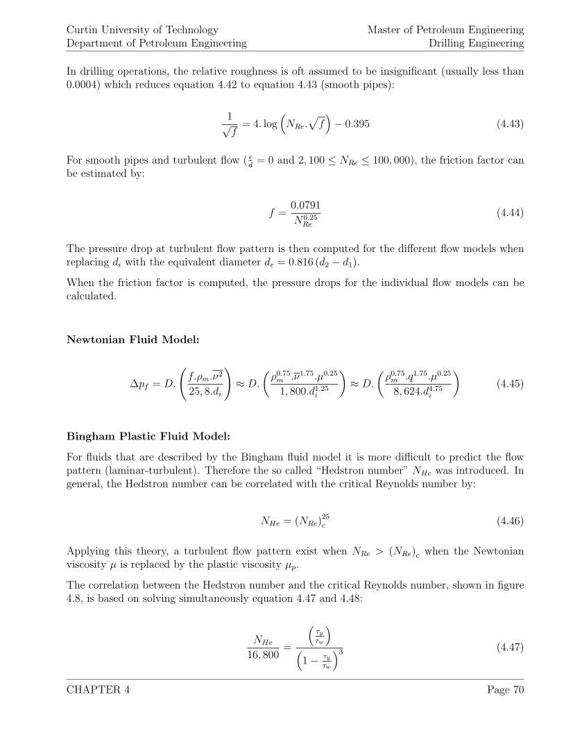
Curtin University of TechnologyDepartment of Petroleum Engineering
Master of Petroleum EngineeringDrilling Engineering
In drilling operations, the relative roughness is oft assumed to be insignificant (usually less than0.0004) which reduces equation 4.42 to equation 4.43 (smooth pipes):
1√f
= 4. log(NRe.
√f)− 0.395 (4.43)
For smooth pipes and turbulent flow ( εd
= 0 and 2, 100 ≤ NRe ≤ 100, 000), the friction factor canbe estimated by:
f =0.0791
N0.25Re
(4.44)
The pressure drop at turbulent flow pattern is then computed for the different flow models whenreplacing di with the equivalent diameter de = 0.816 (d2 − d1).
When the friction factor is computed, the pressure drops for the individual flow models can becalculated.
Newtonian Fluid Model:
∆pf = D.
(f.ρm.ν2
25, 8.di
)≈ D.
(ρ0.75
m .ν1.75.µ0.25
1, 800.d1.25i
)≈ D.
(ρ0.75
m .q1.75.µ0.25
8, 624.d4.75i
)(4.45)
Bingham Plastic Fluid Model:
For fluids that are described by the Bingham fluid model it is more difficult to predict the flowpattern (laminar-turbulent). Therefore the so called “Hedstron number” NHe was introduced. Ingeneral, the Hedstron number can be correlated with the critical Reynolds number by:
NHe = (NRe)25c (4.46)
Applying this theory, a turbulent flow pattern exist when NRe > (NRe)c when the Newtonianviscosity µ is replaced by the plastic viscosity µp.
The correlation between the Hedstron number and the critical Reynolds number, shown in figure4.8, is based on solving simultaneously equation 4.47 and 4.48:
NHe
16, 800=
(τy
τw
)(1 − τy
τw
)3 (4.47)
CHAPTER 4 Page 70
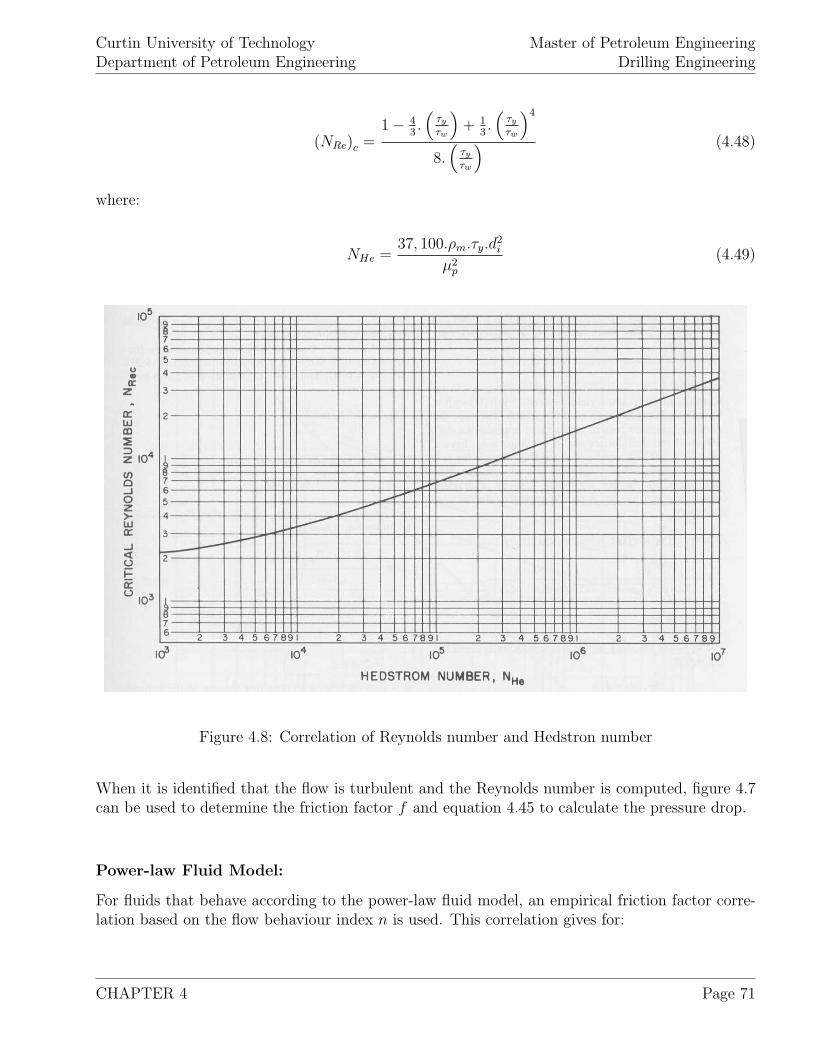
Curtin University of TechnologyDepartment of Petroleum Engineering
Master of Petroleum EngineeringDrilling Engineering
(NRe)c =1 − 4
3.(
τy
τw
)+ 1
3.(
τy
τw
)4
8.(
τy
τw
) (4.48)
where:
NHe =37, 100.ρm.τy.d
2i
µ2p
(4.49)
Figure 4.8: Correlation of Reynolds number and Hedstron number
When it is identified that the flow is turbulent and the Reynolds number is computed, figure 4.7can be used to determine the friction factor f and equation 4.45 to calculate the pressure drop.
Power-law Fluid Model:
For fluids that behave according to the power-law fluid model, an empirical friction factor corre-lation based on the flow behaviour index n is used. This correlation gives for:
CHAPTER 4 Page 71
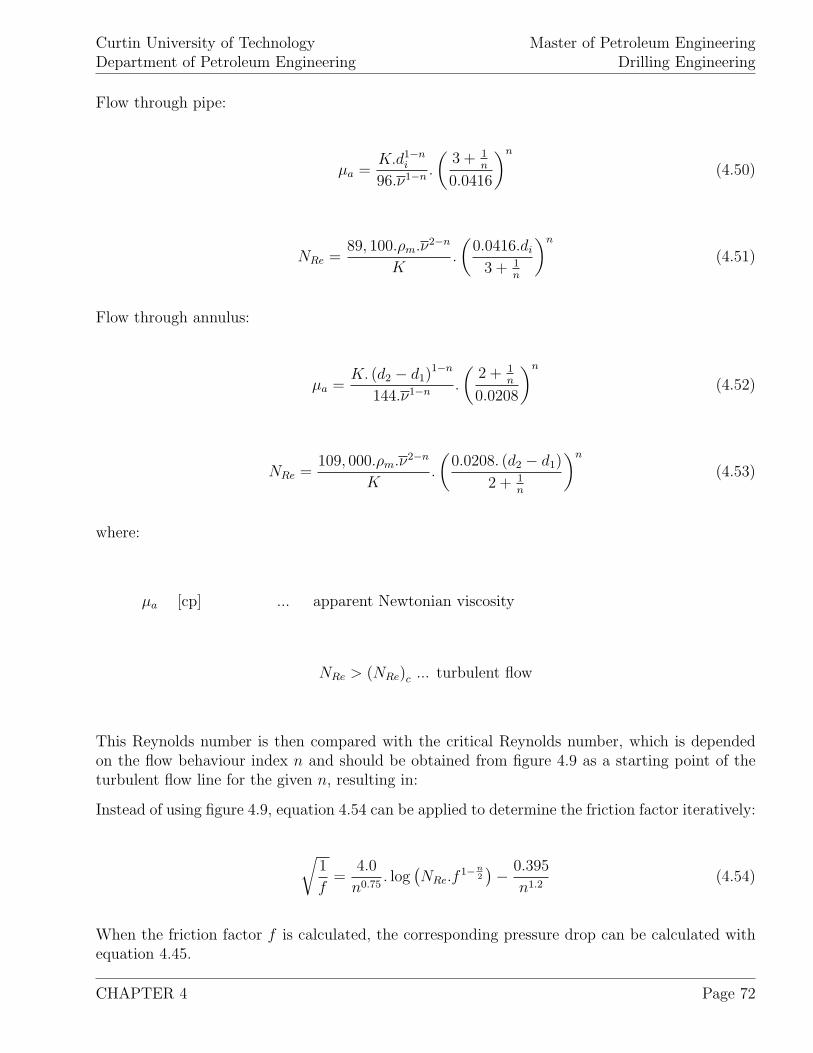
Curtin University of TechnologyDepartment of Petroleum Engineering
Master of Petroleum EngineeringDrilling Engineering
Flow through pipe:
µa =K.d1−n
i
96.ν1−n .
(3 + 1
n
0.0416
)n
(4.50)
NRe =89, 100.ρm.ν2−n
K.
(0.0416.di
3 + 1n
)n
(4.51)
Flow through annulus:
µa =K. (d2 − d1)
1−n
144.ν1−n .
(2 + 1
n
0.0208
)n
(4.52)
NRe =109, 000.ρm.ν2−n
K.
(0.0208. (d2 − d1)
2 + 1n
)n
(4.53)
where:
µa [cp] ... apparent Newtonian viscosity
NRe > (NRe)c ... turbulent flow
This Reynolds number is then compared with the critical Reynolds number, which is dependedon the flow behaviour index n and should be obtained from figure 4.9 as a starting point of theturbulent flow line for the given n, resulting in:
Instead of using figure 4.9, equation 4.54 can be applied to determine the friction factor iteratively:
√1
f=
4.0
n0.75. log
(NRe.f
1−n2
)− 0.395
n1.2(4.54)
When the friction factor f is calculated, the corresponding pressure drop can be calculated withequation 4.45.
CHAPTER 4 Page 72
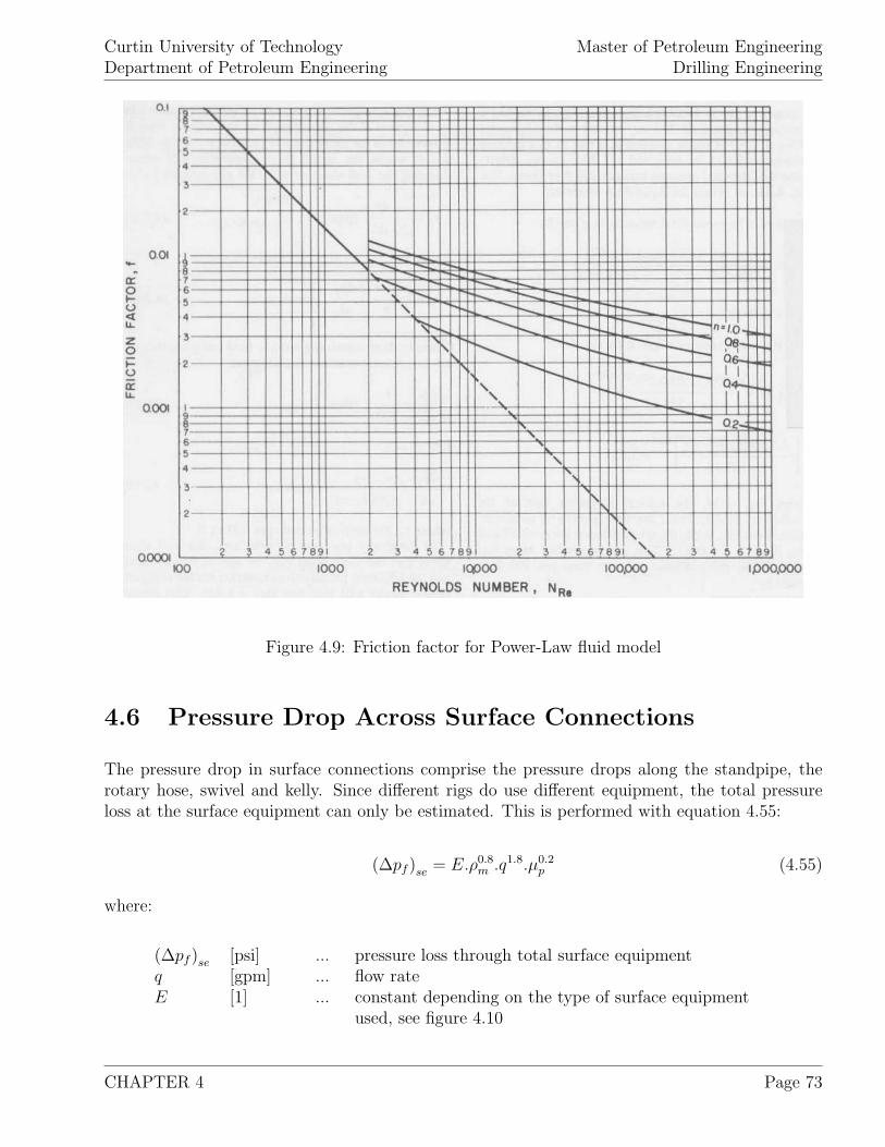
Curtin University of TechnologyDepartment of Petroleum Engineering
Master of Petroleum EngineeringDrilling Engineering
Figure 4.9: Friction factor for Power-Law fluid model
4.6 Pressure Drop Across Surface Connections
The pressure drop in surface connections comprise the pressure drops along the standpipe, therotary hose, swivel and kelly. Since different rigs do use different equipment, the total pressureloss at the surface equipment can only be estimated. This is performed with equation 4.55:
(∆pf )se = E.ρ0.8m .q1.8.µ0.2
p (4.55)
where:
(∆pf )se [psi] ... pressure loss through total surface equipmentq [gpm] ... flow rateE [1] ... constant depending on the type of surface equipment
used, see figure 4.10
CHAPTER 4 Page 73
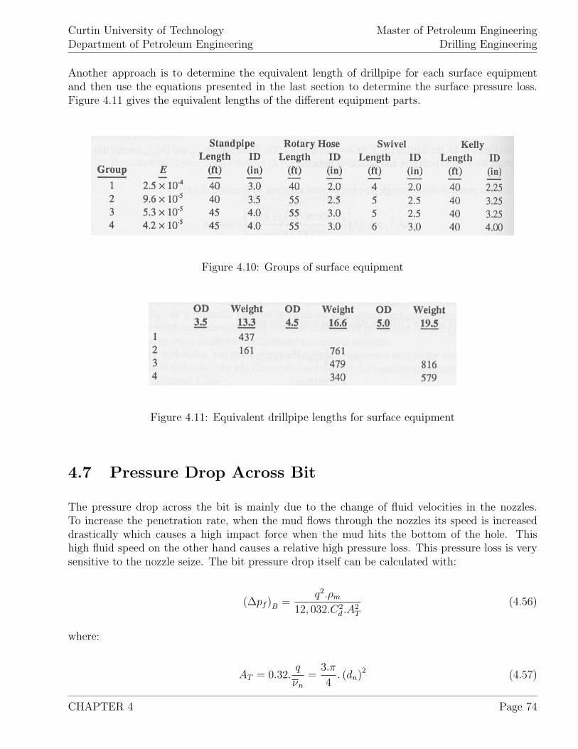
Curtin University of TechnologyDepartment of Petroleum Engineering
Master of Petroleum EngineeringDrilling Engineering
Another approach is to determine the equivalent length of drillpipe for each surface equipmentand then use the equations presented in the last section to determine the surface pressure loss.Figure 4.11 gives the equivalent lengths of the different equipment parts.
Figure 4.10: Groups of surface equipment
Figure 4.11: Equivalent drillpipe lengths for surface equipment
4.7 Pressure Drop Across Bit
The pressure drop across the bit is mainly due to the change of fluid velocities in the nozzles.To increase the penetration rate, when the mud flows through the nozzles its speed is increaseddrastically which causes a high impact force when the mud hits the bottom of the hole. Thishigh fluid speed on the other hand causes a relative high pressure loss. This pressure loss is verysensitive to the nozzle seize. The bit pressure drop itself can be calculated with:
(∆pf )B =q2.ρm
12, 032.C2d .A
2T
(4.56)
where:
AT = 0.32.q
νn
=3.π
4. (dn)2 (4.57)
CHAPTER 4 Page 74
Curtin University of TechnologyDepartment of Petroleum Engineering
Master of Petroleum EngineeringDrilling Engineering
νn = Cd
√1, 238. (∆pf )B
ρm
(4.58)
dn = 32.
√4.AT
3.π(4.59)
AT [in2] ... total nozzle areadn [1/32] ... jet nozzle seizeνn [ft/sec] ... mean nozzle velocityq [gpm] ... flow rateρm [ppg] ... mud densityCd [1] ... discharge coefficient, depending on the nozzle type and
size (commonly Cd = 0.95)
4.8 Initiating Circulation
All the equations to calculate the individual pressure drops presented above assume a non-thixotropic behavior of the mud. In reality, an additional pressure drop is observed when cir-culation is started due to the thixotropic structures which have to be broken down. This initialphase of addition pressure drop may last for one full circulation cycle. The additional pressuredrop can be estimated applying the gel strength τg of the drilling mud as:
For flow through pipes:
(∆pf )p = D.
(τg
300.di
)(4.60)
For flow through annuli:
(∆pf )an = D
[τg
300. (d2 − d1)
](4.61)
where:
τg [lbf/100 ft2] ... gel strength of the drilling mud
CHAPTER 4 Page 75
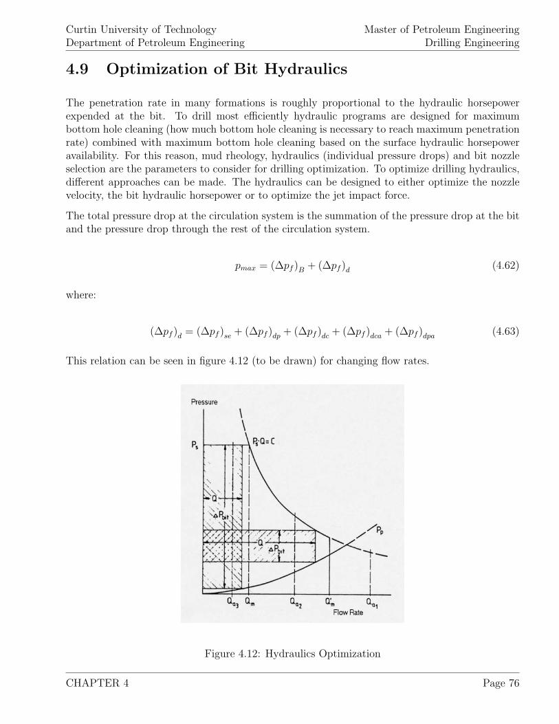
Curtin University of TechnologyDepartment of Petroleum Engineering
Master of Petroleum EngineeringDrilling Engineering
4.9 Optimization of Bit Hydraulics
The penetration rate in many formations is roughly proportional to the hydraulic horsepowerexpended at the bit. To drill most efficiently hydraulic programs are designed for maximumbottom hole cleaning (how much bottom hole cleaning is necessary to reach maximum penetrationrate) combined with maximum bottom hole cleaning based on the surface hydraulic horsepoweravailability. For this reason, mud rheology, hydraulics (individual pressure drops) and bit nozzleselection are the parameters to consider for drilling optimization. To optimize drilling hydraulics,different approaches can be made. The hydraulics can be designed to either optimize the nozzlevelocity, the bit hydraulic horsepower or to optimize the jet impact force.
The total pressure drop at the circulation system is the summation of the pressure drop at the bitand the pressure drop through the rest of the circulation system.
pmax = (∆pf )B + (∆pf )d (4.62)
where:
(∆pf )d = (∆pf )se + (∆pf )dp + (∆pf )dc + (∆pf )dca + (∆pf )dpa (4.63)
This relation can be seen in figure 4.12 (to be drawn) for changing flow rates.
Figure 4.12: Hydraulics Optimization
CHAPTER 4 Page 76
Curtin University of TechnologyDepartment of Petroleum Engineering
Master of Petroleum EngineeringDrilling Engineering
The pressure drop across the bit can be written as:
Hydraulic horsepower:
(∆pf )B−opt = pmax − (∆pf )d−opt = pmax − 1
1 + m.pmax (4.64)
Jet impact force:
(∆pf )B−opt = pmax − (∆pf )d−opt = pmax − 2
2 + m.pmax (4.65)
where:
m [1] ... slope of the parasitic pressure loss (∆pf )d vs. flow rate
Theoretically m = 1.75 but in general it is better to determine m from field data than assumingthis value.
When plotting flow rate vs. pressure on a log-log plot, the optimum design is found at theintersection between the path of optimum hydraulics and the (∆pf )d line for either of the criteriamentioned above.
Having determined the optimum design, the optimum pump flow rate, optimum nozzle area andcorresponding pressure losses can be calculated:
(AT )opt =
√(qopt)
2 .ρm
12, 032.C2d . (∆pf )B−opt
(4.66)
(dn)opt = 32.
√4. (AT )opt
3.π(4.67)
Optimum hydraulic horsepower and jet impact force are given with:
(hp)opt =(∆pf )B−opt .qopt
1, 714(4.68)
(Fj)opt = 0.01823.Cd.qopt.√
ρm. (∆pf )B−opt (4.69)
The optimum nozzle area leads to the respective nozzle selection. Nozzles for drilling bits are given132
[in] seizes thus the calculated nozzle area has to be converted into n32
[in]. Knowing n (has to
CHAPTER 4 Page 77
Curtin University of TechnologyDepartment of Petroleum Engineering
Master of Petroleum EngineeringDrilling Engineering
be an integer and is commonly rounded down to ensure the nozzle velocity) and the amount ofnozzles to use, the individual seizes are found.
The so called “specific hydraulic horsepower” is defined as hydraulic horsepower per unit boreholecross-section.
(hp)spec =4.hp
π.d2BH
(4.70)
The optimization as discussed above is performed for regular intervals (e.g. 1,000 [ft]) and isincluded in the drilling program. In practice, computer programs are available in the industrythat perform these hydraulic optimization calculations.
4.10 Particle Slip Velocity
The annular flow of the drilling fluid carrying drilling cuttings and a certain amount of gas to thesurface, is disturbed by frictional and centrifugal forces caused by the rotation of the drillstring.In practice, when it is noticed that inefficient hole cleaning is present, either the mud flow rate isincreased or the effective viscosity of the mud is increased or both adjustments are performed.
To estimate the slip velocity of the cuttings, following correlation methods were developed empir-ically and are widely accepted and used in the industry:
Moore’s Correlation:
µa =K
144.
(d2 − d1
νan
)1−n
.
(2 + 1
n
0.0208
)n
(4.71)
for NRp > 300:
νsl = 1.54.
√ds.
ρs − ρm
ρm
(4.72)
for NRp < 3:
νsl = 82.87.d2
s
µa
. (ρs − ρm) (4.73)
for 3 ≤ NRp < 300:
νsl =2.90.ds. (ρs − ρm)0.667
ρ0.333m .µ0.333
a
(4.74)
CHAPTER 4 Page 78
Curtin University of TechnologyDepartment of Petroleum Engineering
Master of Petroleum EngineeringDrilling Engineering
where:
NRp =928.ρm.νsl.ds
µa
(4.75)
ds =τg
10.4. (ρs − ρm)(4.76)
µa [cp] ... apparent Newtonian viscosityds [in] ... drilling cuttings diameterNRp [1] ... particle Reynolds numberνsl [ft/sec] ... particle slip velocityρs [ppg] ... cuttings densityτg [lbf/100 ft2] ... gel strength required to suspend a particle of diameter ds
Chien’s Correlation:
The correlation equations determined by Chien are similar to the ones defined by Moore. Forclay-water muds, he recommends the usage of the apparent viscosity.
µa = µp + 5.τy.ds
νa
(4.77)
The correlation is performed as:
for NRp < 100:
νsl = 0.0075.
(µa
ρm.ds
).
√√√√36, 800.ds(
µa
ρm.ds
)2 .
(ρs − ρm
ρm
)+ 1 − 1
(4.78)
for NRp > 100:
νsl = 1.44.d2
s
µa
(ρs − ρm) (4.79)
The so called “transportation velocity” νT is defined as the difference between the mean annularvelocity νan and the slip velocity νsl. The “transportation ratio” FT given by:
FT =νT
νan
(4.80)
CHAPTER 4 Page 79
Curtin University of TechnologyDepartment of Petroleum Engineering
Master of Petroleum EngineeringDrilling Engineering
determines whether the cuttings are transported to the surface (FT is positive) or not and providesa relative measure of the carrying capability of the drilling mud.
To have proper hole cleaning and with the knowledge of the transport velocity, a minimum meanannular velocity can be determined. This minimum mean annular velocity has to be calculated atthe annulus with the maximum cross-section area and in this way determines the minimum pumprate. As a rule of thumb, a minimum mean annular velocity of 3 [ft/sec] is often applied.
4.11 Surge and Swab Pressure
When running tubulars in a hole filled with drilling mud so called “surge pressures” and “swabpressures” are created. The surge pressure is an increase of the pressure in front of the tubularswhen run into the well, the swab pressure is a pressure reduction behind the tubular when pulledout of the well. Excessive surge or swab pressures have to be avoided since they can lead toproblems like:
1. Pressure reduction due to swab can cause a kick,
2. Pressure increase due to surge pressure can fracture weaker formation and cause lost circu-lation which in turn can cause a kick,
3. Swab pressure increases the intake of formation gas (trip gas) which in turn can decreasethe hydrostatic pressure.
The parameters that determine surge and swab pressures are: mud rheological properties, tubularvelocity, tubular and hole geometry. The mean annular fluid velocity caused by tubular movementis by definition positive when moved upward and negative when moved downward. It is calculatedfor:
closed tubulars:
νan−closed = νp.
(0.45 +
d2p
d2h − d2
p
)(4.81)
open tubulars:
νan−open = νp.
(0.45 +
d2p − d2
i
d2h − d2
p + d2i
)(4.82)
νmax = 1.5.νan (4.83)
The corresponding pressure drop is calculated assuming the power-law model and the correspond-ing factors n and K:
CHAPTER 4 Page 80
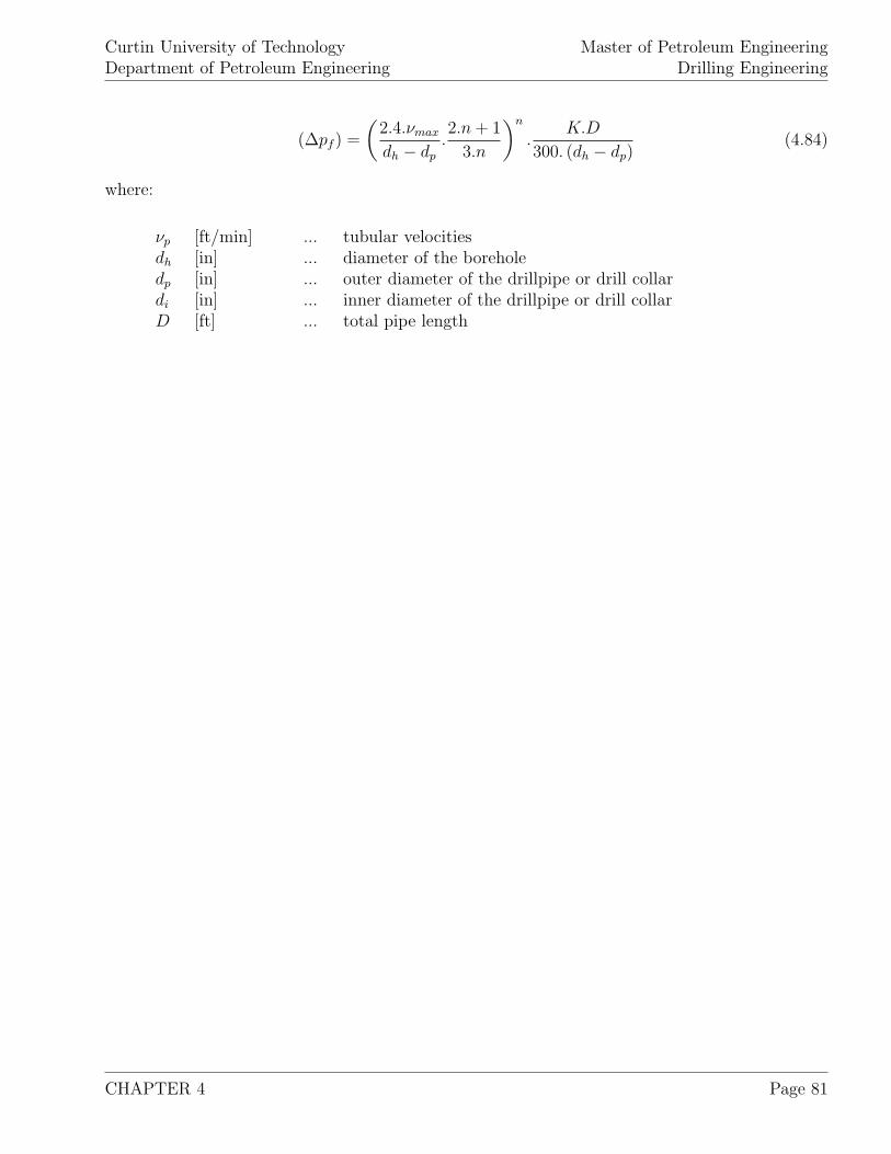
Curtin University of TechnologyDepartment of Petroleum Engineering
Master of Petroleum EngineeringDrilling Engineering
(∆pf ) =
(2.4.νmax
dh − dp
.2.n + 1
3.n
)n
.K.D
300. (dh − dp)(4.84)
where:
νp [ft/min] ... tubular velocitiesdh [in] ... diameter of the boreholedp [in] ... outer diameter of the drillpipe or drill collardi [in] ... inner diameter of the drillpipe or drill collarD [ft] ... total pipe length
CHAPTER 4 Page 81
Curtin University of TechnologyDepartment of Petroleum Engineering
Master of Petroleum EngineeringDrilling Engineering
4.12 Examples
1. To cement a casing string at a depth of 8,500 [ft] the used 10 [ppg] drilling mud is to bedisplaced from the annulus by a 600 [ft] preflush of 9 [ppg] mud, 1,800 [ft] of 12.5 [ppg] fillercement and 1,600 [ft] of 16.0 [ppg] high-strength cement. After the high-strength cement, brinewith 8.5 [ppg] is pumped as spacer. Compute the:
(a) Minimum pump pressure required to completelydisplace the casing,
(b) Equivalent mud weight at 8,500 [ft] after the cementhas been displaced completely from the casing.
2. A non-Newtonian fluid is measured by a rotation viscosimeter giving readings of 22 at 300[rpm] and 39 at 600 [rpm] respectively. When the fluid is characterised by the Bingham plasticfluid model, µp and τy is to be determined, when the power-law model is applied, the consistencyand flow behavior index have to be computed.
3. A fluid characterized by the Bingham plastic fluid model has a yield point of 12 [lbf/ 100 ft]and a plastic viscosity of 50 [cp]. When the flow pattern is laminar, the pressure drop due tofriction at 8,000 [ft] is to be computed for a:
(a) flow rate of 50 [gpm] through a drillstringwith 3.826 [in] ID,
(b) flow rate of 90 [gpm] through a 10 X 7 [in]annulus.
4. When drilling a well to 1,000 [ft], a Bingham plastic fluid with a yield point of 5 [lbf/ 100 ft]and plastic viscosity of 25 [cp] is applied. Using following additional information (Ldp = 1, 000[ft], di = 3.826 [in], d1 = 4.5 [in], d2 = 6.5 [in], q = 500 [gpm], ε
d= 0) calculate the:
(a) Flow pattern in the drillpipe,(b) Flow pattern in the annulus opposite the drillpipe,(c) Frictional pressure loss in the drillpipe,(d) Frictional pressure loss in the annulus.
5. Assuming the same mean flow velocities and a power-law fluid model with a consistency indexof 200 [eq cp] and flow behavior index of 0.75, calculate the same values at in example 4.
CHAPTER 4 Page 82
Curtin University of TechnologyDepartment of Petroleum Engineering
Master of Petroleum EngineeringDrilling Engineering
6. A jet bit shall produce a 800 [psi] pressure drop through the nozzles when circulating 900 [gpm]of 10 [ppg] drilling mud. Select 3 nozzles that produce this pressure drop and calculate the jetvelocity of the mud.
7. A 11.75 [in] casing with a closed end is lowered into a 12.25 [in] hole at a rate of 1.5 [ft/sec].What is the equivalent density below the bottom joint at 7,000 [ft] when the hole is filled with a10.5 [ppg] mud having a viscosity of 2.5 [cp]?
8. When drilling with a 10 [ppg] mud and a bit, using three 1232
[in] nozzles, the pump pressureat a flow rate of 500 [gpm] is 3,000 [psi]. When the frow rate is dropped to 250 [gpm], a pumppressure of 800 [psi] is recorded. The minimum flow rate to lift the cuttings is determined as 240[gpm], the maximum allowable surface pressure is 3,000 [psi]. The pump itself is rated at 1,000[hp] and exhibits an overall efficiency of 90 %. Compute the:
(a) Proper operating conditions and bit nozzle sizes formaximum bit horsepower for the next bit run¿,
(b) Bit horsepower required to obtain the conditions selected,(c) Jet impact force obtained at the conditions selected,(d) Jet nozzle velocity obtained at the conditions selected.
CHAPTER 4 Page 83

Curtin University of TechnologyDepartment of Petroleum Engineering
Master of Petroleum EngineeringDrilling Engineering
CHAPTER 4 Page 84
Curtin University of TechnologyDepartment of Petroleum Engineering
Master of Petroleum EngineeringDrilling Engineering
Chapter 5
Drilling Bits
Drill bit selection is in general a complicated process but, when performed properly, has a majorimpact on the total well cost. First in this chapter, the different types of drill bits are discussed.Then, applying their classification and wear considerations, a drill bit selection is presented.Finally, various parameters that influence the rate of penetration are discussed.
5.1 Drill Bit Types
5.1.1 Roller Cone Bit
Roller cone bits comprise one, two or three cones having teeth sticking out of them. A roller conebit with three cones is the most often applied type of drilling bit. Typical roller cone bits areshown in figure 5.1.
The cutting action of this bit can be described as follows: when the bit is rotated at the bottomof the hole, the teeth are pressed onto the formation below the bit and applies a force exceedingthe compressive strength of the rock. This is sketched in figure 5.2.
Some of the advantages of roller cone bits over fixed cutter bits are:
(a) Can handle rough drilling conditions,(b) Less expensive than fixed cutter bits,(c) Are more sensitive to the amount of pressure overbalance and thus
better indicator of overpressure formations,
The gauge of the hole drilled by roller cone bits is maintained by the outside cutters whichare also known as “gauge cutters”. These teeth are very vulnerable to wear that increases inabrasive sandstone formations. When the gauge cutters are worn out, the consequent hole drilled
CHAPTER 5 Page 85
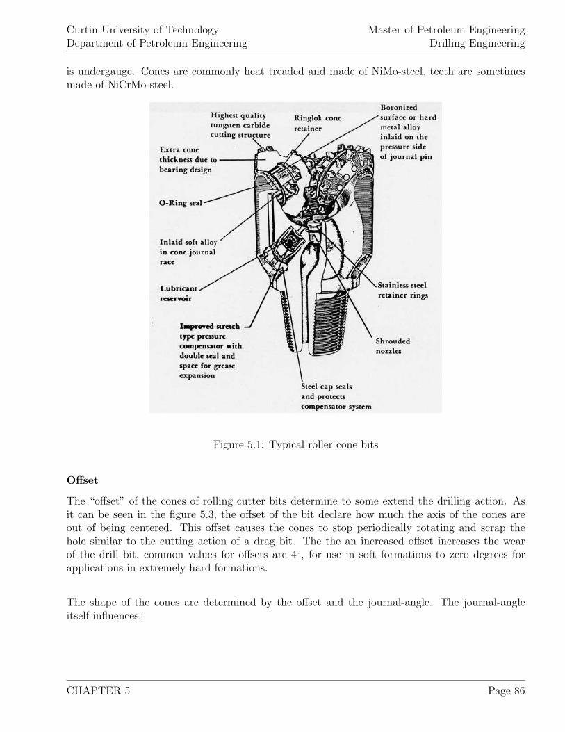
Curtin University of TechnologyDepartment of Petroleum Engineering
Master of Petroleum EngineeringDrilling Engineering
is undergauge. Cones are commonly heat treaded and made of NiMo-steel, teeth are sometimesmade of NiCrMo-steel.
Figure 5.1: Typical roller cone bits
Offset
The “offset” of the cones of rolling cutter bits determine to some extend the drilling action. Asit can be seen in the figure 5.3, the offset of the bit declare how much the axis of the cones areout of being centered. This offset causes the cones to stop periodically rotating and scrap thehole similar to the cutting action of a drag bit. The the an increased offset increases the wearof the drill bit, common values for offsets are 4◦, for use in soft formations to zero degrees forapplications in extremely hard formations.
The shape of the cones are determined by the offset and the journal-angle. The journal-angleitself influences:
CHAPTER 5 Page 86
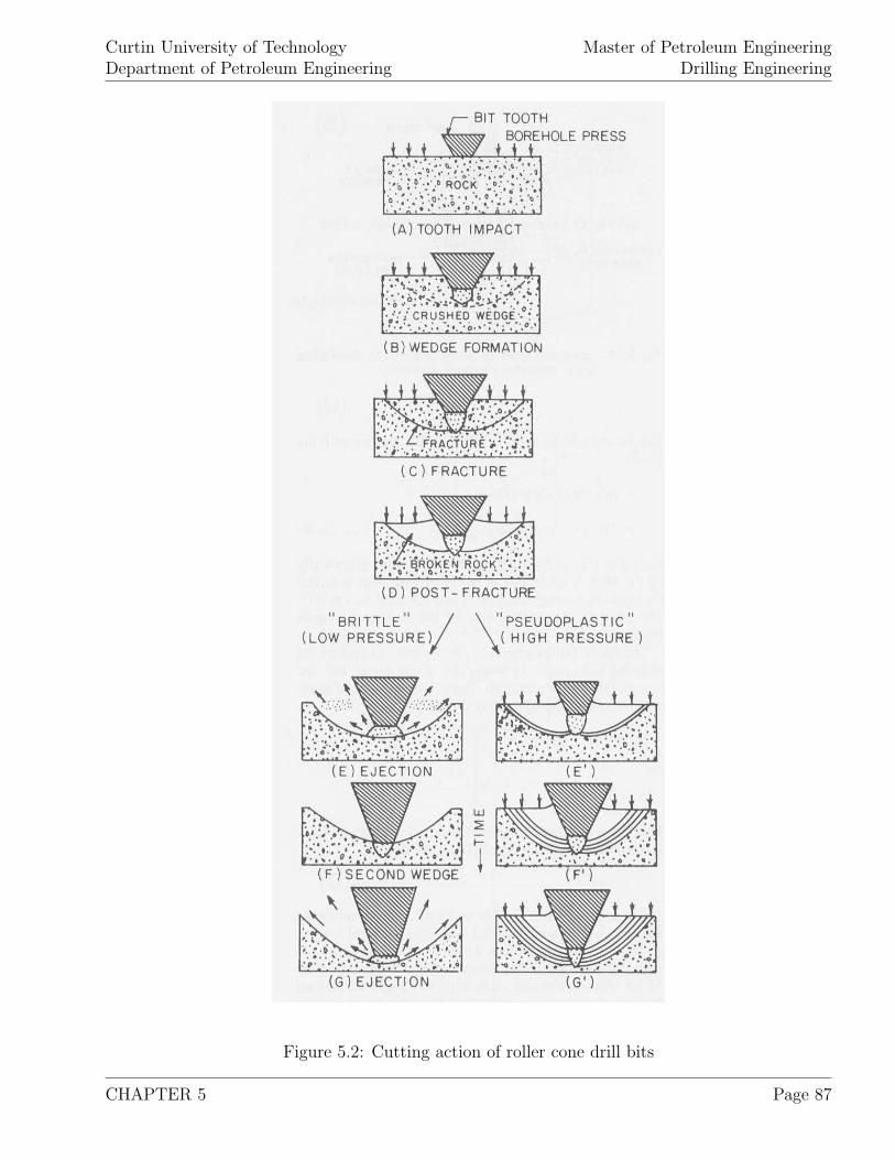
Curtin University of TechnologyDepartment of Petroleum Engineering
Master of Petroleum EngineeringDrilling Engineering
Figure 5.2: Cutting action of roller cone drill bits
CHAPTER 5 Page 87
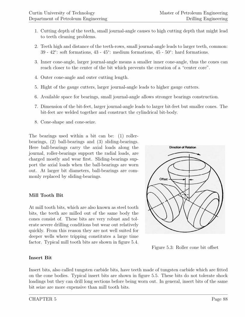
Curtin University of TechnologyDepartment of Petroleum Engineering
Master of Petroleum EngineeringDrilling Engineering
1. Cutting depth of the teeth, small journal-angle causes to high cutting depth that might leadto teeth cleaning problems.
2. Teeth high and distance of the teeth-rows, small journal-angle leads to larger teeth, common:39 - 42◦: soft formations, 43 - 45◦: medium formations, 45 - 50◦: hard formations.
3. Inner cone-angle, larger journal-angle means a smaller inner cone-angle, thus the cones canreach closer to the center of the bit which prevents the creation of a “center core”.
4. Outer cone-angle and outer cutting length.
5. Hight of the gauge cutters, larger journal-angle leads to higher gauge cutters.
6. Available space for bearings, small journal-angle allows stronger bearings construction.
7. Dimension of the bit-feet, larger journal-angle leads to larger bit-feet but smaller cones. Thebit-feet are welded together and construct the cylindrical bit-body.
8. Cone-shape and cone-seize.
Figure 5.3: Roller cone bit offset
The bearings used within a bit can be: (1) roller-bearings, (2) ball-bearings and (3) sliding-bearings.Here ball-bearings carry the axial loads along thejournal, roller-bearings support the radial loads, arecharged mostly and wear first. Sliding-bearings sup-port the axial loads when the ball-bearings are wornout. At larger bit diameters, ball-bearings are com-monly replaced by sliding-bearings.
Mill Tooth Bit
At mill tooth bits, which are also known as steel toothbits, the teeth are milled out of the same body thecones consist of. These bits are very robust and tol-erate severe drilling conditions but wear out relativelyquickly. From this reason they are not well suited fordeeper wells where tripping constitutes a large timefactor. Typical mill tooth bits are shown in figure 5.4.
Insert Bit
Insert bits, also called tungsten carbide bits, have teeth made of tungsten carbide which are fittedon the cone bodies. Typical insert bits are shown in figure 5.5. These bits do not tolerate shockloadings but they can drill long sections before being worn out. In general, insert bits of the samebit seize are more expensive than mill tooth bits.
CHAPTER 5 Page 88
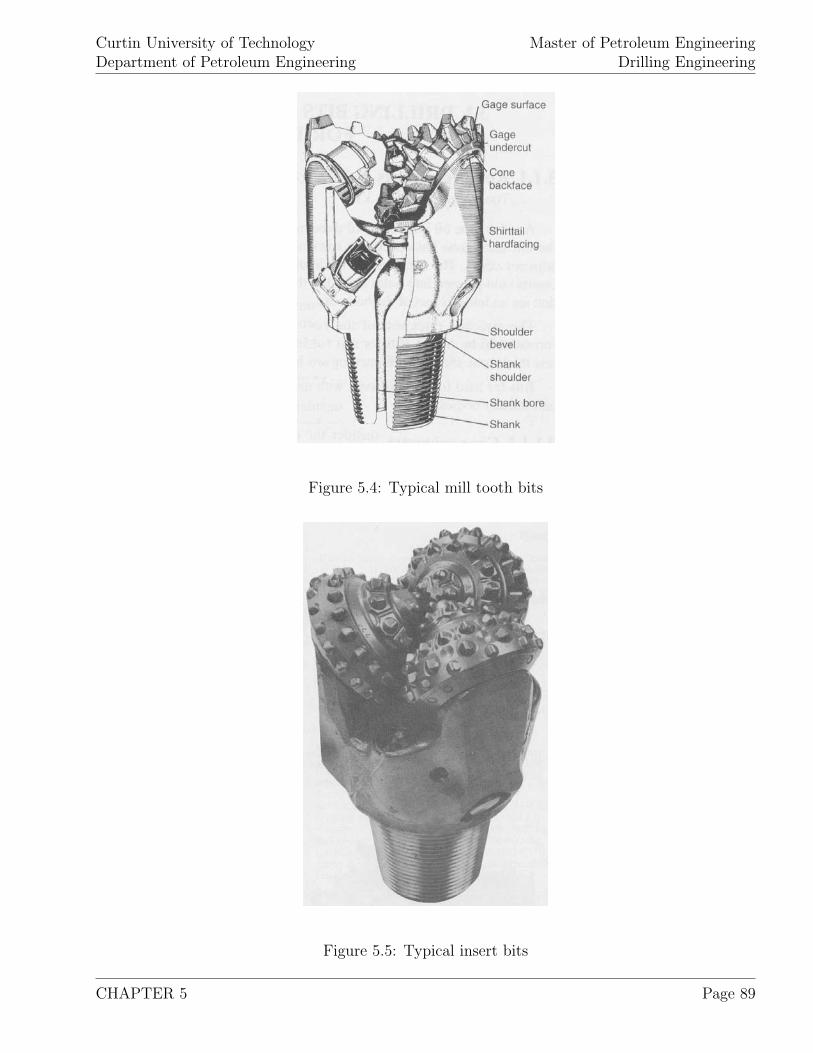
Curtin University of TechnologyDepartment of Petroleum Engineering
Master of Petroleum EngineeringDrilling Engineering
Figure 5.4: Typical mill tooth bits
Figure 5.5: Typical insert bits
CHAPTER 5 Page 89
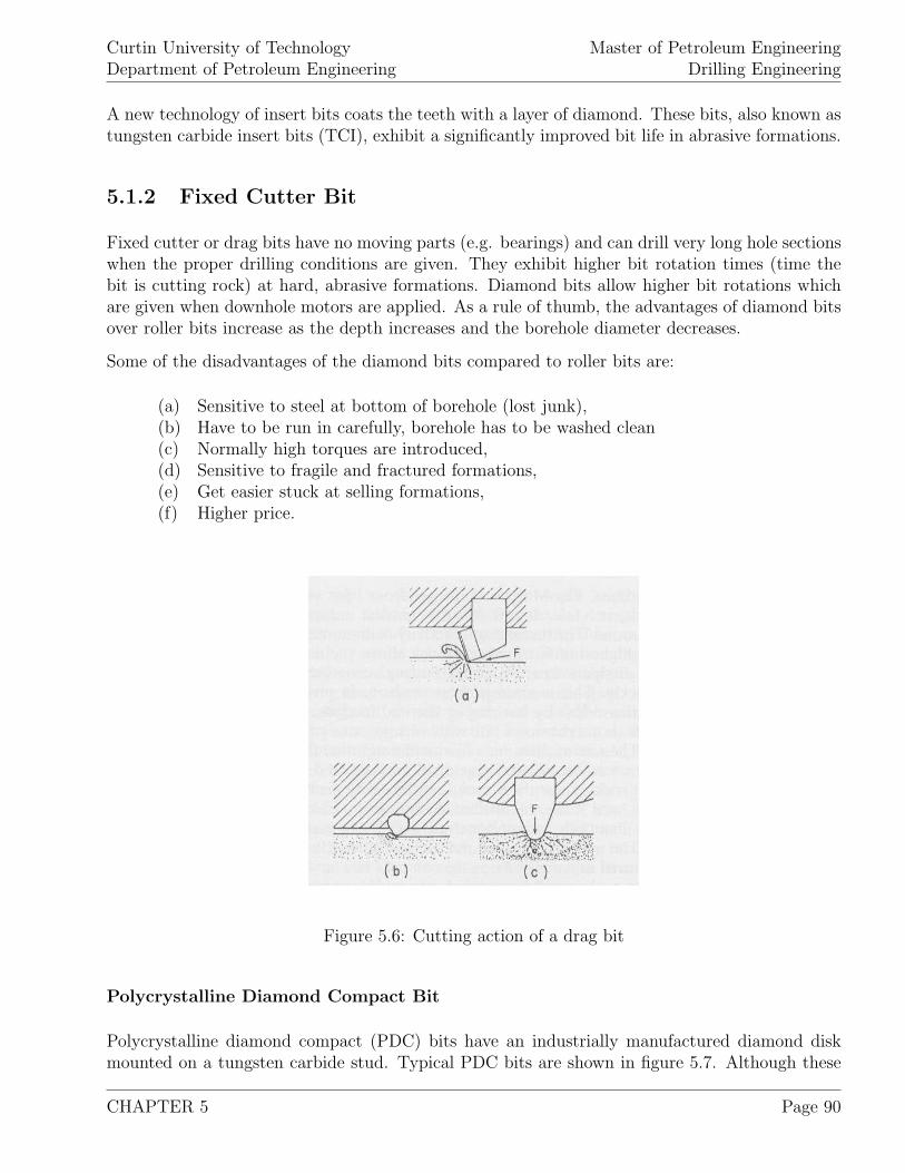
Curtin University of TechnologyDepartment of Petroleum Engineering
Master of Petroleum EngineeringDrilling Engineering
A new technology of insert bits coats the teeth with a layer of diamond. These bits, also known astungsten carbide insert bits (TCI), exhibit a significantly improved bit life in abrasive formations.
5.1.2 Fixed Cutter Bit
Fixed cutter or drag bits have no moving parts (e.g. bearings) and can drill very long hole sectionswhen the proper drilling conditions are given. They exhibit higher bit rotation times (time thebit is cutting rock) at hard, abrasive formations. Diamond bits allow higher bit rotations whichare given when downhole motors are applied. As a rule of thumb, the advantages of diamond bitsover roller bits increase as the depth increases and the borehole diameter decreases.
Some of the disadvantages of the diamond bits compared to roller bits are:
(a) Sensitive to steel at bottom of borehole (lost junk),(b) Have to be run in carefully, borehole has to be washed clean(c) Normally high torques are introduced,(d) Sensitive to fragile and fractured formations,(e) Get easier stuck at selling formations,(f) Higher price.
Figure 5.6: Cutting action of a drag bit
Polycrystalline Diamond Compact Bit
Polycrystalline diamond compact (PDC) bits have an industrially manufactured diamond diskmounted on a tungsten carbide stud. Typical PDC bits are shown in figure 5.7. Although these
CHAPTER 5 Page 90
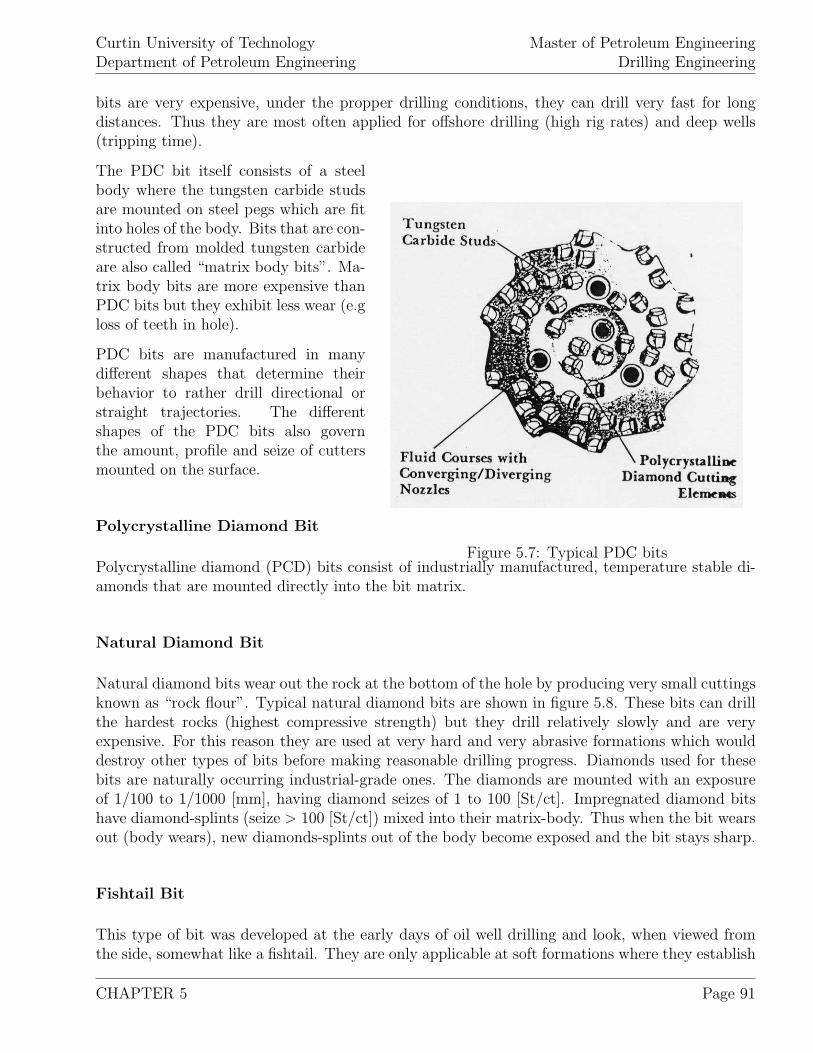
Curtin University of TechnologyDepartment of Petroleum Engineering
Master of Petroleum EngineeringDrilling Engineering
bits are very expensive, under the propper drilling conditions, they can drill very fast for longdistances. Thus they are most often applied for offshore drilling (high rig rates) and deep wells(tripping time).
Figure 5.7: Typical PDC bits
The PDC bit itself consists of a steelbody where the tungsten carbide studsare mounted on steel pegs which are fitinto holes of the body. Bits that are con-structed from molded tungsten carbideare also called “matrix body bits”. Ma-trix body bits are more expensive thanPDC bits but they exhibit less wear (e.gloss of teeth in hole).
PDC bits are manufactured in manydifferent shapes that determine theirbehavior to rather drill directional orstraight trajectories. The differentshapes of the PDC bits also governthe amount, profile and seize of cuttersmounted on the surface.
Polycrystalline Diamond Bit
Polycrystalline diamond (PCD) bits consist of industrially manufactured, temperature stable di-amonds that are mounted directly into the bit matrix.
Natural Diamond Bit
Natural diamond bits wear out the rock at the bottom of the hole by producing very small cuttingsknown as “rock flour”. Typical natural diamond bits are shown in figure 5.8. These bits can drillthe hardest rocks (highest compressive strength) but they drill relatively slowly and are veryexpensive. For this reason they are used at very hard and very abrasive formations which woulddestroy other types of bits before making reasonable drilling progress. Diamonds used for thesebits are naturally occurring industrial-grade ones. The diamonds are mounted with an exposureof 1/100 to 1/1000 [mm], having diamond seizes of 1 to 100 [St/ct]. Impregnated diamond bitshave diamond-splints (seize > 100 [St/ct]) mixed into their matrix-body. Thus when the bit wearsout (body wears), new diamonds-splints out of the body become exposed and the bit stays sharp.
Fishtail Bit
This type of bit was developed at the early days of oil well drilling and look, when viewed fromthe side, somewhat like a fishtail. They are only applicable at soft formations where they establish
CHAPTER 5 Page 91
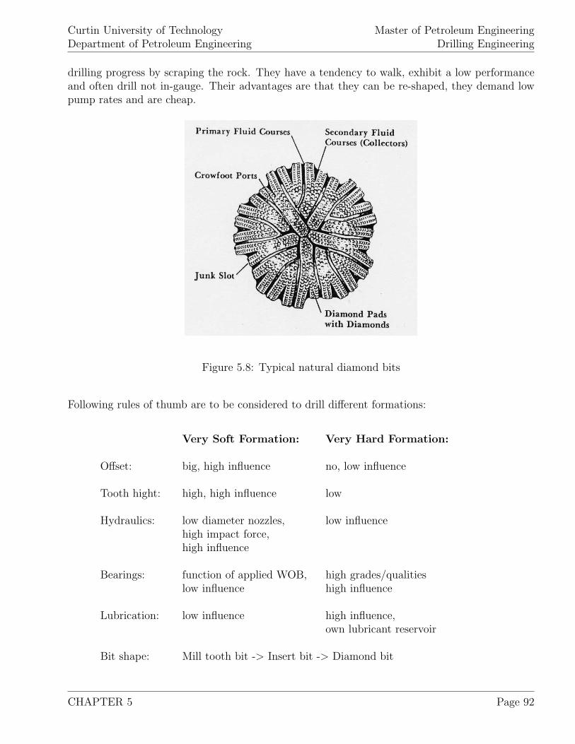
Curtin University of TechnologyDepartment of Petroleum Engineering
Master of Petroleum EngineeringDrilling Engineering
drilling progress by scraping the rock. They have a tendency to walk, exhibit a low performanceand often drill not in-gauge. Their advantages are that they can be re-shaped, they demand lowpump rates and are cheap.
Figure 5.8: Typical natural diamond bits
Following rules of thumb are to be considered to drill different formations:
Very Soft Formation: Very Hard Formation:
Offset: big, high influence no, low influence
Tooth hight: high, high influence low
Hydraulics: low diameter nozzles, low influencehigh impact force,high influence
Bearings: function of applied WOB, high grades/qualitieslow influence high influence
Lubrication: low influence high influence,own lubricant reservoir
Bit shape: Mill tooth bit -> Insert bit -> Diamond bit
CHAPTER 5 Page 92
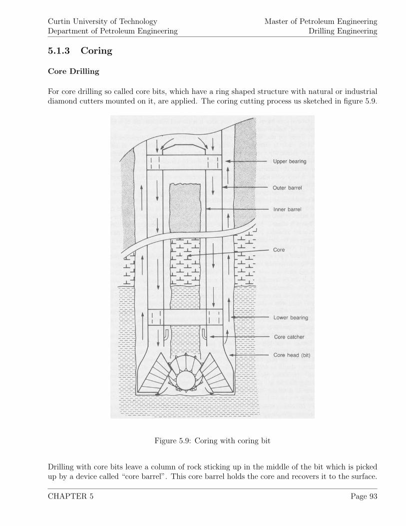
Curtin University of TechnologyDepartment of Petroleum Engineering
Master of Petroleum EngineeringDrilling Engineering
5.1.3 Coring
Core Drilling
For core drilling so called core bits, which have a ring shaped structure with natural or industrialdiamond cutters mounted on it, are applied. The coring cutting process us sketched in figure 5.9.
Figure 5.9: Coring with coring bit
Drilling with core bits leave a column of rock sticking up in the middle of the bit which is pickedup by a device called “core barrel”. This core barrel holds the core and recovers it to the surface.
CHAPTER 5 Page 93
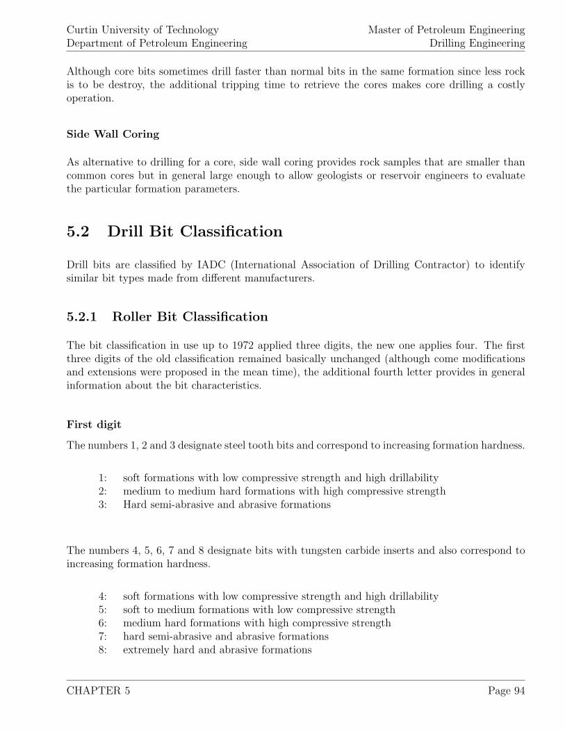
Curtin University of TechnologyDepartment of Petroleum Engineering
Master of Petroleum EngineeringDrilling Engineering
Although core bits sometimes drill faster than normal bits in the same formation since less rockis to be destroy, the additional tripping time to retrieve the cores makes core drilling a costlyoperation.
Side Wall Coring
As alternative to drilling for a core, side wall coring provides rock samples that are smaller thancommon cores but in general large enough to allow geologists or reservoir engineers to evaluatethe particular formation parameters.
5.2 Drill Bit Classification
Drill bits are classified by IADC (International Association of Drilling Contractor) to identifysimilar bit types made from different manufacturers.
5.2.1 Roller Bit Classification
The bit classification in use up to 1972 applied three digits, the new one applies four. The firstthree digits of the old classification remained basically unchanged (although come modificationsand extensions were proposed in the mean time), the additional fourth letter provides in generalinformation about the bit characteristics.
First digit
The numbers 1, 2 and 3 designate steel tooth bits and correspond to increasing formation hardness.
1: soft formations with low compressive strength and high drillability2: medium to medium hard formations with high compressive strength3: Hard semi-abrasive and abrasive formations
The numbers 4, 5, 6, 7 and 8 designate bits with tungsten carbide inserts and also correspond toincreasing formation hardness.
4: soft formations with low compressive strength and high drillability5: soft to medium formations with low compressive strength6: medium hard formations with high compressive strength7: hard semi-abrasive and abrasive formations8: extremely hard and abrasive formations
CHAPTER 5 Page 94
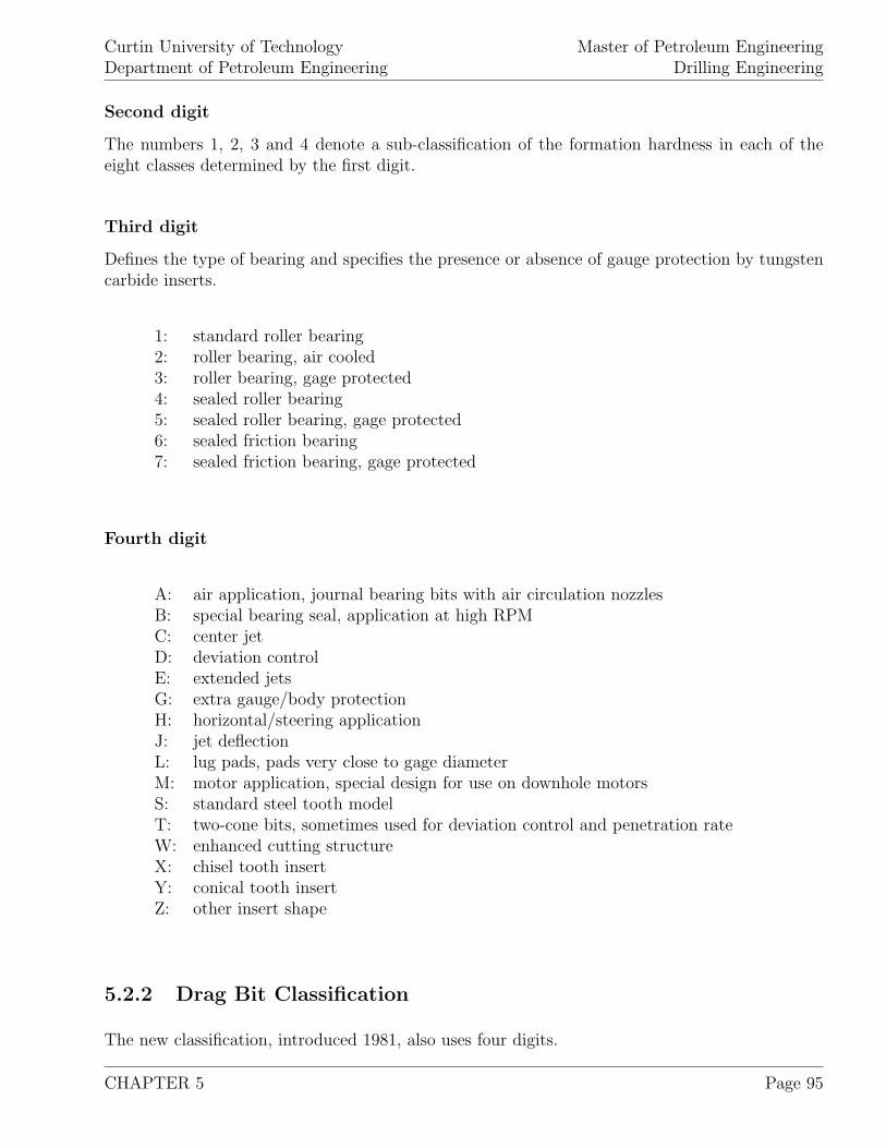
Curtin University of TechnologyDepartment of Petroleum Engineering
Master of Petroleum EngineeringDrilling Engineering
Second digit
The numbers 1, 2, 3 and 4 denote a sub-classification of the formation hardness in each of theeight classes determined by the first digit.
Third digit
Defines the type of bearing and specifies the presence or absence of gauge protection by tungstencarbide inserts.
1: standard roller bearing2: roller bearing, air cooled3: roller bearing, gage protected4: sealed roller bearing5: sealed roller bearing, gage protected6: sealed friction bearing7: sealed friction bearing, gage protected
Fourth digit
A: air application, journal bearing bits with air circulation nozzlesB: special bearing seal, application at high RPMC: center jetD: deviation controlE: extended jetsG: extra gauge/body protectionH: horizontal/steering applicationJ: jet deflectionL: lug pads, pads very close to gage diameterM: motor application, special design for use on downhole motorsS: standard steel tooth modelT: two-cone bits, sometimes used for deviation control and penetration rateW: enhanced cutting structureX: chisel tooth insertY: conical tooth insertZ: other insert shape
5.2.2 Drag Bit Classification
The new classification, introduced 1981, also uses four digits.
CHAPTER 5 Page 95
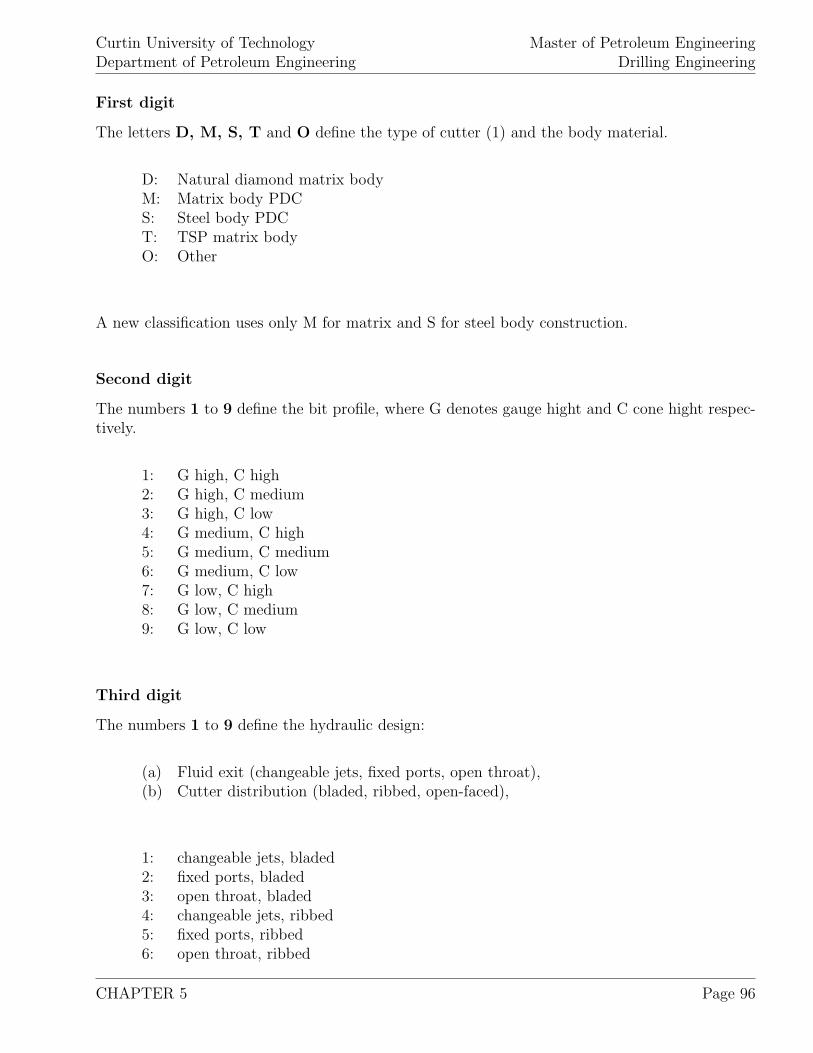
Curtin University of TechnologyDepartment of Petroleum Engineering
Master of Petroleum EngineeringDrilling Engineering
First digit
The letters D, M, S, T and O define the type of cutter (1) and the body material.
D: Natural diamond matrix bodyM: Matrix body PDCS: Steel body PDCT: TSP matrix bodyO: Other
A new classification uses only M for matrix and S for steel body construction.
Second digit
The numbers 1 to 9 define the bit profile, where G denotes gauge hight and C cone hight respec-tively.
1: G high, C high2: G high, C medium3: G high, C low4: G medium, C high5: G medium, C medium6: G medium, C low7: G low, C high8: G low, C medium9: G low, C low
Third digit
The numbers 1 to 9 define the hydraulic design:
(a) Fluid exit (changeable jets, fixed ports, open throat),(b) Cutter distribution (bladed, ribbed, open-faced),
1: changeable jets, bladed2: fixed ports, bladed3: open throat, bladed4: changeable jets, ribbed5: fixed ports, ribbed6: open throat, ribbed
CHAPTER 5 Page 96
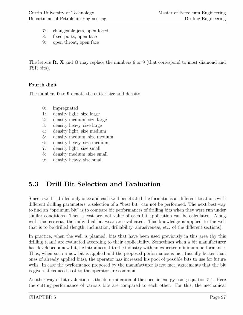
Curtin University of TechnologyDepartment of Petroleum Engineering
Master of Petroleum EngineeringDrilling Engineering
7: changeable jets, open faced8: fixed ports, open face9: open throat, open face
The letters R, X and O may replace the numbers 6 or 9 (that correspond to most diamond andTSR bits).
Fourth digit
The numbers 0 to 9 denote the cutter size and density.
0: impregnated1: density light, size large2: density medium, size large3: density heavy, size large4: density light, size medium5: density medium, size medium6: density heavy, size medium7: density light, size small8: density medium, size small9: density heavy, size small
5.3 Drill Bit Selection and Evaluation
Since a well is drilled only once and each well penetrated the formations at different locations withdifferent drilling parameters, a selection of a “best bit” can not be performed. The next best wayto find an “optimum bit” is to compare bit performances of drilling bits when they were run undersimilar conditions. Then a cost-per-foot value of each bit application can be calculated. Alongwith this criteria, the individual bit wear are evaluated. This knowledge is applied to the wellthat is to be drilled (length, inclination, drillability, abrasiveness, etc. of the different sections).
In practice, when the well is planned, bits that have been used previously in this area (by thisdrilling team) are evaluated according to their applicability. Sometimes when a bit manufacturerhas developed a new bit, he introduces it to the industry with an expected minimum performance.Thus, when such a new bit is applied and the proposed performance is met (usually better thanones of already applied bits), the operator has increased his pool of possible bits to use for futurewells. In case the performance proposed by the manufacturer is not met, agreements that the bitis given at reduced cost to the operator are common.
Another way of bit evaluation is the determination of the specific energy using equation 5.1. Herethe cutting-performance of various bits are compared to each other. For this, the mechanical
CHAPTER 5 Page 97
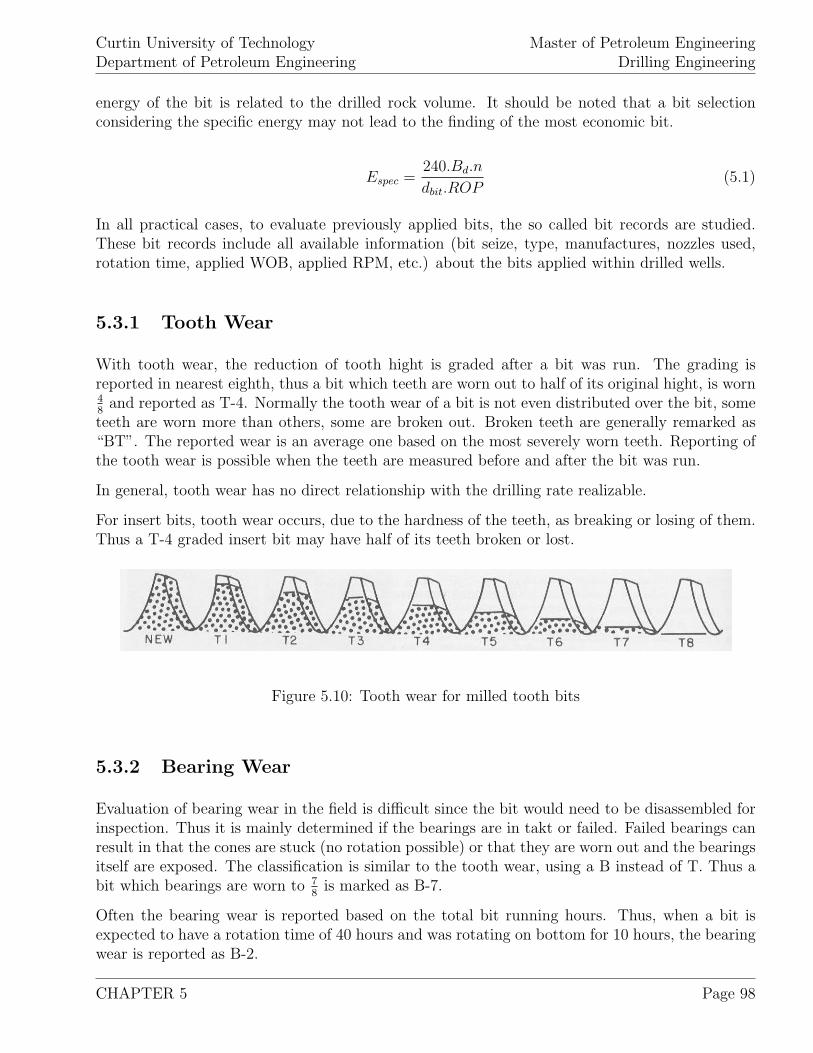
Curtin University of TechnologyDepartment of Petroleum Engineering
Master of Petroleum EngineeringDrilling Engineering
energy of the bit is related to the drilled rock volume. It should be noted that a bit selectionconsidering the specific energy may not lead to the finding of the most economic bit.
Espec =240.Bd.n
dbit.ROP(5.1)
In all practical cases, to evaluate previously applied bits, the so called bit records are studied.These bit records include all available information (bit seize, type, manufactures, nozzles used,rotation time, applied WOB, applied RPM, etc.) about the bits applied within drilled wells.
5.3.1 Tooth Wear
With tooth wear, the reduction of tooth hight is graded after a bit was run. The grading isreported in nearest eighth, thus a bit which teeth are worn out to half of its original hight, is worn48
and reported as T-4. Normally the tooth wear of a bit is not even distributed over the bit, someteeth are worn more than others, some are broken out. Broken teeth are generally remarked as“BT”. The reported wear is an average one based on the most severely worn teeth. Reporting ofthe tooth wear is possible when the teeth are measured before and after the bit was run.
In general, tooth wear has no direct relationship with the drilling rate realizable.
For insert bits, tooth wear occurs, due to the hardness of the teeth, as breaking or losing of them.Thus a T-4 graded insert bit may have half of its teeth broken or lost.
Figure 5.10: Tooth wear for milled tooth bits
5.3.2 Bearing Wear
Evaluation of bearing wear in the field is difficult since the bit would need to be disassembled forinspection. Thus it is mainly determined if the bearings are in takt or failed. Failed bearings canresult in that the cones are stuck (no rotation possible) or that they are worn out and the bearingsitself are exposed. The classification is similar to the tooth wear, using a B instead of T. Thus abit which bearings are worn to 7
8is marked as B-7.
Often the bearing wear is reported based on the total bit running hours. Thus, when a bit isexpected to have a rotation time of 40 hours and was rotating on bottom for 10 hours, the bearingwear is reported as B-2.
CHAPTER 5 Page 98
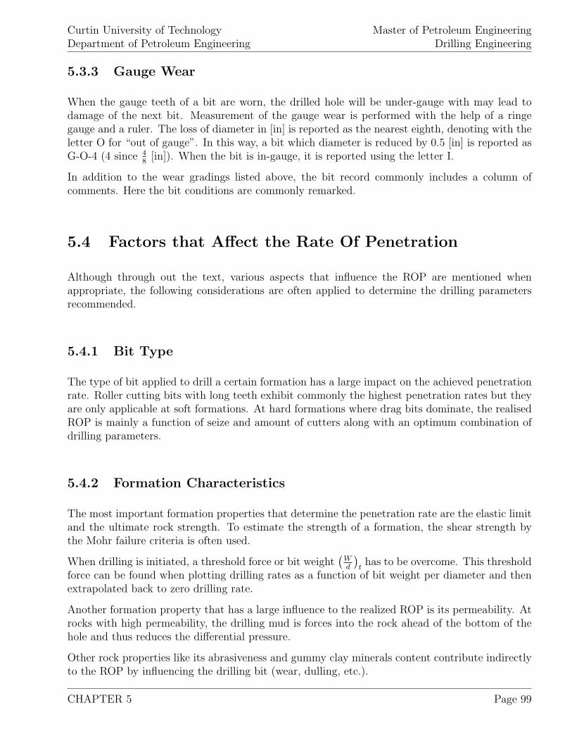
Curtin University of TechnologyDepartment of Petroleum Engineering
Master of Petroleum EngineeringDrilling Engineering
5.3.3 Gauge Wear
When the gauge teeth of a bit are worn, the drilled hole will be under-gauge with may lead todamage of the next bit. Measurement of the gauge wear is performed with the help of a ringegauge and a ruler. The loss of diameter in [in] is reported as the nearest eighth, denoting with theletter O for “out of gauge”. In this way, a bit which diameter is reduced by 0.5 [in] is reported asG-O-4 (4 since 4
8[in]). When the bit is in-gauge, it is reported using the letter I.
In addition to the wear gradings listed above, the bit record commonly includes a column ofcomments. Here the bit conditions are commonly remarked.
5.4 Factors that Affect the Rate Of Penetration
Although through out the text, various aspects that influence the ROP are mentioned whenappropriate, the following considerations are often applied to determine the drilling parametersrecommended.
5.4.1 Bit Type
The type of bit applied to drill a certain formation has a large impact on the achieved penetrationrate. Roller cutting bits with long teeth exhibit commonly the highest penetration rates but theyare only applicable at soft formations. At hard formations where drag bits dominate, the realisedROP is mainly a function of seize and amount of cutters along with an optimum combination ofdrilling parameters.
5.4.2 Formation Characteristics
The most important formation properties that determine the penetration rate are the elastic limitand the ultimate rock strength. To estimate the strength of a formation, the shear strength bythe Mohr failure criteria is often used.
When drilling is initiated, a threshold force or bit weight(
Wd
)thas to be overcome. This threshold
force can be found when plotting drilling rates as a function of bit weight per diameter and thenextrapolated back to zero drilling rate.
Another formation property that has a large influence to the realized ROP is its permeability. Atrocks with high permeability, the drilling mud is forces into the rock ahead of the bottom of thehole and thus reduces the differential pressure.
Other rock properties like its abrasiveness and gummy clay minerals content contribute indirectlyto the ROP by influencing the drilling bit (wear, dulling, etc.).
CHAPTER 5 Page 99
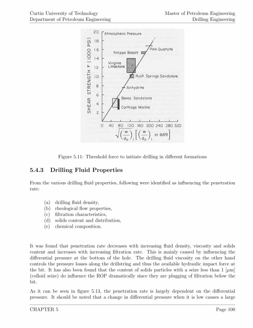
Curtin University of TechnologyDepartment of Petroleum Engineering
Master of Petroleum EngineeringDrilling Engineering
Figure 5.11: Threshold force to initiate drilling in different formations
5.4.3 Drilling Fluid Properties
From the various drilling fluid properties, following were identified as influencing the penetrationrate:
(a) drilling fluid density,(b) rheological flow properties,(c) filtration characteristics,(d) solids content and distribution,(e) chemical composition.
It was found that penetration rate decreases with increasing fluid density, viscosity and solidscontent and increases with increasing filtration rate. This is mainly caused by influencing thedifferential pressure at the bottom of the hole. The drilling fluid viscosity on the other handcontrols the pressure losses along the drillstring and thus the available hydraulic impact force atthe bit. It has also been found that the content of solids particles with a seize less than 1 [µm](colloid seize) do influence the ROP dramatically since they are plugging of filtration below thebit.
As it can be seen in figure 5.13, the penetration rate is largely dependent on the differentialpressure. It should be noted that a change in differential pressure when it is low causes a large
CHAPTER 5 Page 100
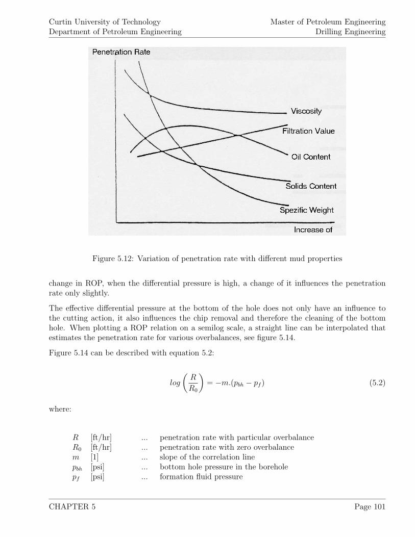
Curtin University of TechnologyDepartment of Petroleum Engineering
Master of Petroleum EngineeringDrilling Engineering
Figure 5.12: Variation of penetration rate with different mud properties
change in ROP, when the differential pressure is high, a change of it influences the penetrationrate only slightly.
The effective differential pressure at the bottom of the hole does not only have an influence tothe cutting action, it also influences the chip removal and therefore the cleaning of the bottomhole. When plotting a ROP relation on a semilog scale, a straight line can be interpolated thatestimates the penetration rate for various overbalances, see figure 5.14.
Figure 5.14 can be described with equation 5.2:
log
(R
R0
)= −m.(pbh − pf ) (5.2)
where:
R [ft/hr] ... penetration rate with particular overbalanceR0 [ft/hr] ... penetration rate with zero overbalancem [1] ... slope of the correlation linepbh [psi] ... bottom hole pressure in the boreholepf [psi] ... formation fluid pressure
CHAPTER 5 Page 101
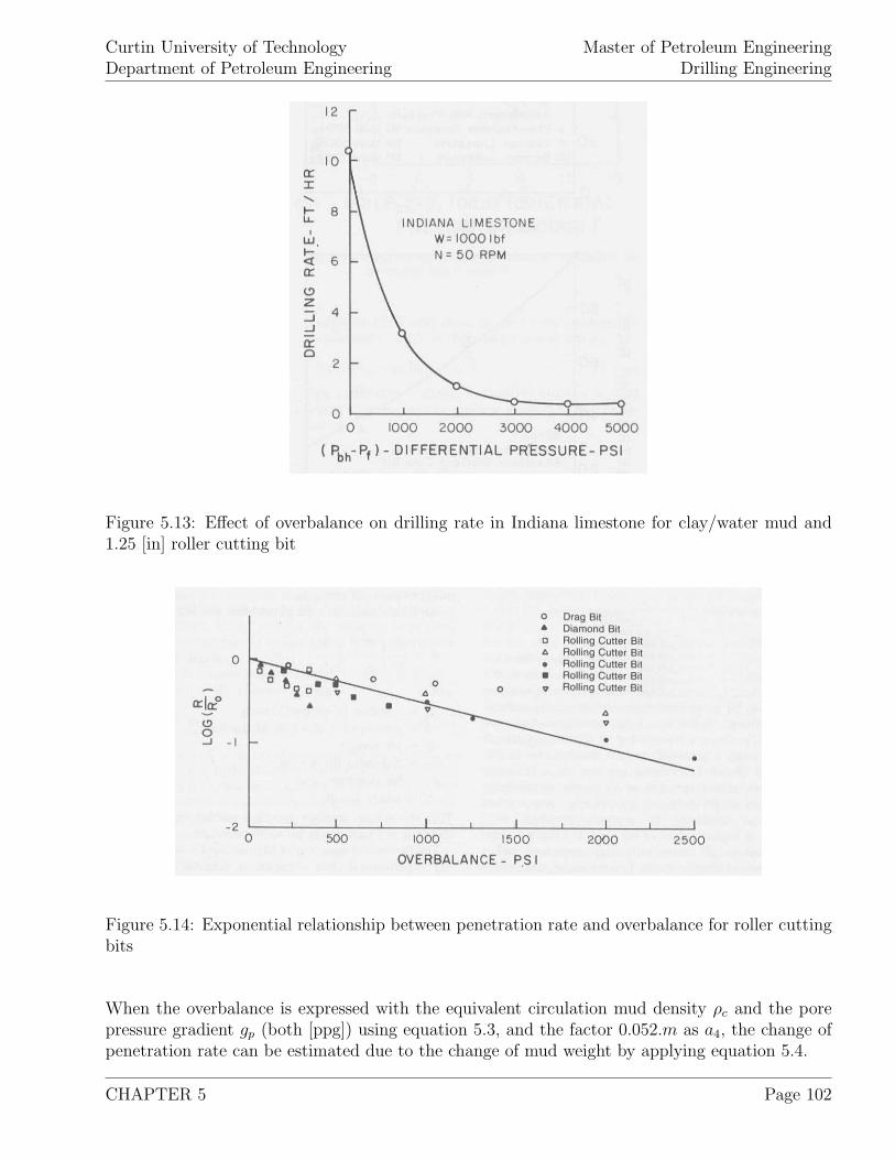
Curtin University of TechnologyDepartment of Petroleum Engineering
Master of Petroleum EngineeringDrilling Engineering
Figure 5.13: Effect of overbalance on drilling rate in Indiana limestone for clay/water mud and1.25 [in] roller cutting bit
Figure 5.14: Exponential relationship between penetration rate and overbalance for roller cuttingbits
When the overbalance is expressed with the equivalent circulation mud density ρc and the porepressure gradient gp (both [ppg]) using equation 5.3, and the factor 0.052.m as a4, the change ofpenetration rate can be estimated due to the change of mud weight by applying equation 5.4.
CHAPTER 5 Page 102
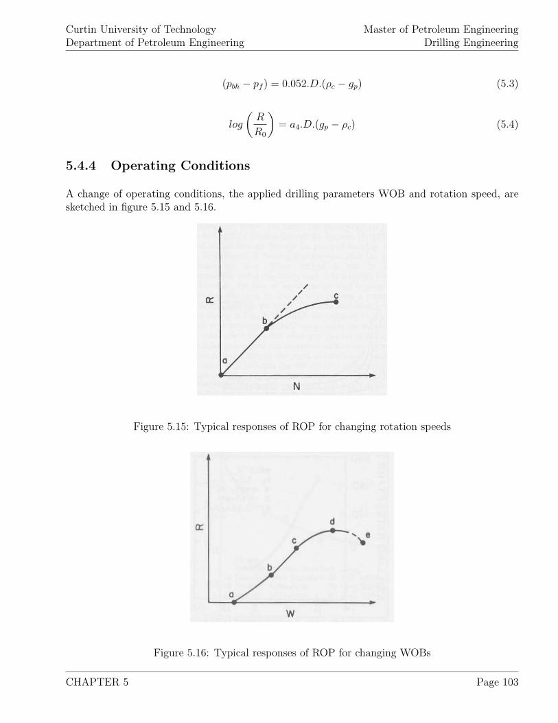
Curtin University of TechnologyDepartment of Petroleum Engineering
Master of Petroleum EngineeringDrilling Engineering
(pbh − pf ) = 0.052.D.(ρc − gp) (5.3)
log
(R
R0
)= a4.D.(gp − ρc) (5.4)
5.4.4 Operating Conditions
A change of operating conditions, the applied drilling parameters WOB and rotation speed, aresketched in figure 5.15 and 5.16.
Figure 5.15: Typical responses of ROP for changing rotation speeds
Figure 5.16: Typical responses of ROP for changing WOBs
CHAPTER 5 Page 103
Curtin University of TechnologyDepartment of Petroleum Engineering
Master of Petroleum EngineeringDrilling Engineering
The decreased ROP, when WOB is increased (section d-e at figure ??) is called “bit floundering”and is attributed to less efficient bottom hole cleaning.
A so called “Drill-off-test” can be applied to determine the drillability of a homogenous formationand to optimize the applied drilling parameters. To carry out a drill-off-test, the maximum WOBis applied along with a constant RPM. Then the time until the bit drills free is counted. When thisprocedure is repeated with various speeds, a WOB-time diagram can be developed, repeating theprocedure with various WOBs, the optimum WOB-RPM combinations can be found. It shouldbe noted that the drill-off-test has to be carried out within a homogenous formation and since ittakes a relatively long time, it is performed very seldom.
5.4.5 Bit Wear
As the bit is worn during drilling, the penetration rate decreases. This reduction of ROP isgenerally less severe for insert bits as for milled tooth bits.
5.4.6 Bit Hydraulics
Practice has shown that effective bit hydraulics can improve the penetration rate dramatically.The enhanced jetting action promotes a better cleaning of the teeth as well as the bottom of thehole. To improve the cleaning capacity of the bit extended nozzles are often applied where thedischarging nozzle ends are closer to the hole bottom. When extended nozzles are mounted onthe drilling bit, a center jet must also be used to prevent bit balling in soft formations.
As discussed with well hydraulics, hydraulic horsepower, jet impact force and nozzle velocities arethe criteria to optimize hydraulics. When a low WOB is applied and drilling rates are low, therequired hydraulics for efficient hole cleaning is small. When the WOB is increased and the wellis drilled faster, efficient hydraulic programs have to be followed to realize the higher penetrationrates.
CHAPTER 5 Page 104

Curtin University of TechnologyDepartment of Petroleum Engineering
Master of Petroleum EngineeringDrilling Engineering
5.5 Examples
CHAPTER 5 Page 105

Curtin University of TechnologyDepartment of Petroleum Engineering
Master of Petroleum EngineeringDrilling Engineering
CHAPTER 5 Page 106
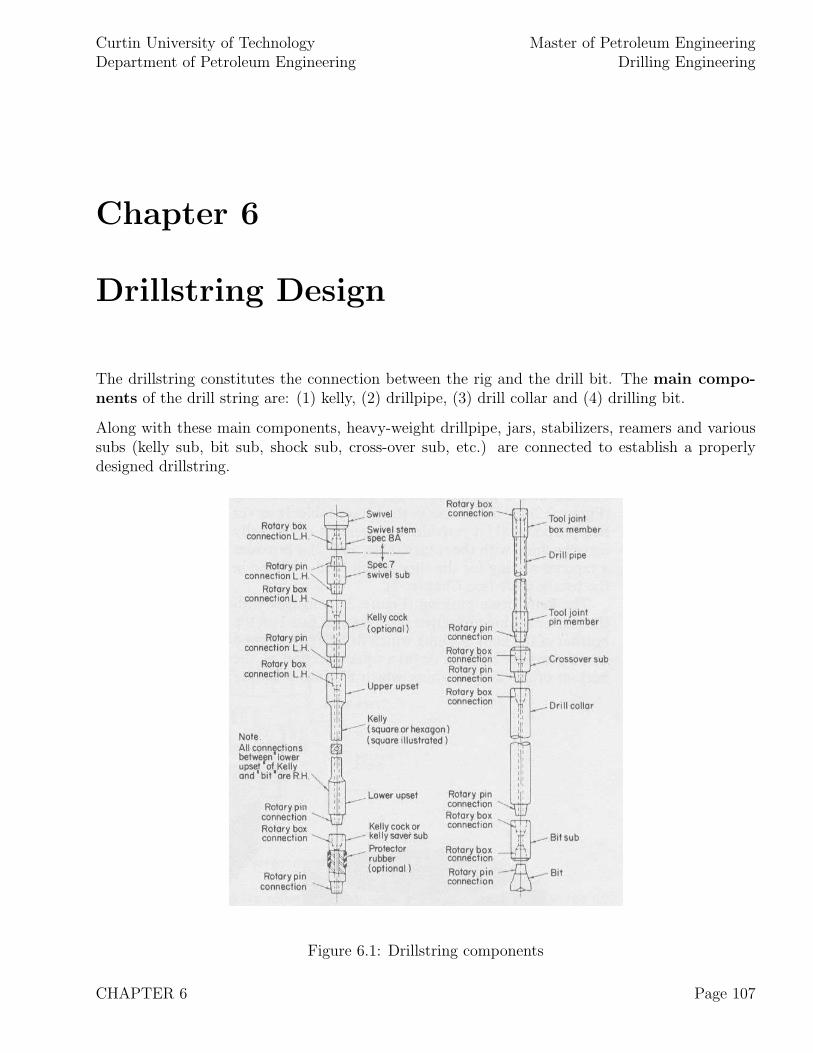
Curtin University of TechnologyDepartment of Petroleum Engineering
Master of Petroleum EngineeringDrilling Engineering
Chapter 6
Drillstring Design
The drillstring constitutes the connection between the rig and the drill bit. The main compo-nents of the drill string are: (1) kelly, (2) drillpipe, (3) drill collar and (4) drilling bit.
Along with these main components, heavy-weight drillpipe, jars, stabilizers, reamers and varioussubs (kelly sub, bit sub, shock sub, cross-over sub, etc.) are connected to establish a properlydesigned drillstring.
Figure 6.1: Drillstring components
CHAPTER 6 Page 107
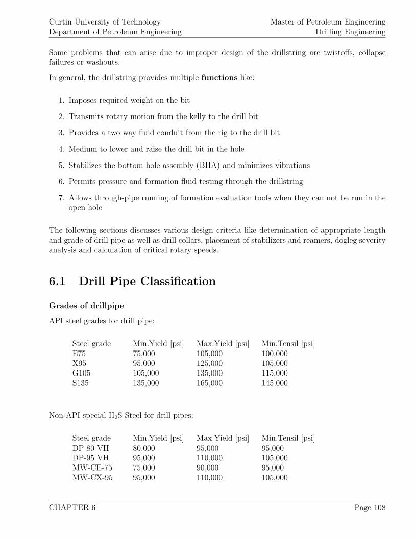
Curtin University of TechnologyDepartment of Petroleum Engineering
Master of Petroleum EngineeringDrilling Engineering
Some problems that can arise due to improper design of the drillstring are twistoffs, collapsefailures or washouts.
In general, the drillstring provides multiple functions like:
1. Imposes required weight on the bit
2. Transmits rotary motion from the kelly to the drill bit
3. Provides a two way fluid conduit from the rig to the drill bit
4. Medium to lower and raise the drill bit in the hole
5. Stabilizes the bottom hole assembly (BHA) and minimizes vibrations
6. Permits pressure and formation fluid testing through the drillstring
7. Allows through-pipe running of formation evaluation tools when they can not be run in theopen hole
The following sections discusses various design criteria like determination of appropriate lengthand grade of drill pipe as well as drill collars, placement of stabilizers and reamers, dogleg severityanalysis and calculation of critical rotary speeds.
6.1 Drill Pipe Classification
Grades of drillpipe
API steel grades for drill pipe:
Steel grade Min.Yield [psi] Max.Yield [psi] Min.Tensil [psi]E75 75,000 105,000 100,000X95 95,000 125,000 105,000G105 105,000 135,000 115,000S135 135,000 165,000 145,000
Non-API special H2S Steel for drill pipes:
Steel grade Min.Yield [psi] Max.Yield [psi] Min.Tensil [psi]DP-80 VH 80,000 95,000 95,000DP-95 VH 95,000 110,000 105,000MW-CE-75 75,000 90,000 95,000MW-CX-95 95,000 110,000 105,000
CHAPTER 6 Page 108
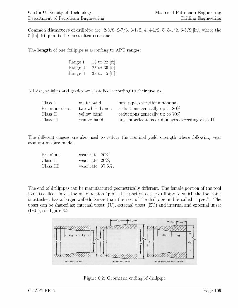
Curtin University of TechnologyDepartment of Petroleum Engineering
Master of Petroleum EngineeringDrilling Engineering
Common diameters of drillpipe are: 2-3/8, 2-7/8, 3-1/2, 4, 4-1/2, 5, 5-1/2, 6-5/8 [in], where the5 [in] drillpipe is the most often used one.
The length of one drillpipe is according to APT ranges:
Range 1 18 to 22 [ft]Range 2 27 to 30 [ft]Range 3 38 to 45 [ft]
All size, weights and grades are classified according to their use as:
Class I white band new pipe, everything nominalPremium class two white bands reductions generally up to 80%Class II yellow band reductions generally up to 70%Class III orange band any imperfections or damages exceeding class II
The different classes are also used to reduce the nominal yield strength where following wearassumptions are made:
Premium wear rate: 20%,Class II wear rate: 20%,Class III wear rate: 37.5%,
The end of drillpipes can be manufactured geometrically different. The female portion of the tooljoint is called “box”, the male portion “pin”. The portion of the drillpipe to which the tool jointis attached has a larger wall-thickness than the rest of the drillpipe and is called “upset”. Theupset can be shaped as: internal upset (IU), external upset (EU) and internal and external upset(IEU), see figure 6.2.
Figure 6.2: Geometric ending of drillpipe
CHAPTER 6 Page 109
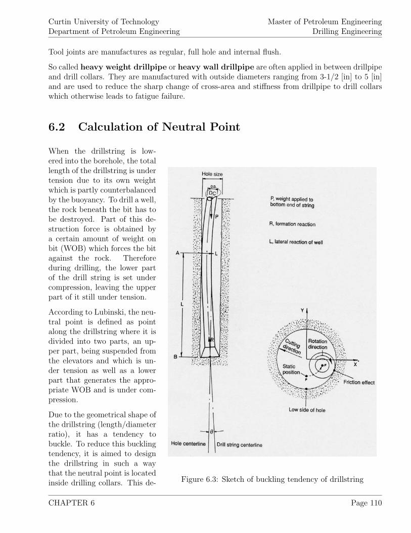
Curtin University of TechnologyDepartment of Petroleum Engineering
Master of Petroleum EngineeringDrilling Engineering
Tool joints are manufactures as regular, full hole and internal flush.
So called heavy weight drillpipe or heavy wall drillpipe are often applied in between drillpipeand drill collars. They are manufactured with outside diameters ranging from 3-1/2 [in] to 5 [in]and are used to reduce the sharp change of cross-area and stiffness from drillpipe to drill collarswhich otherwise leads to fatigue failure.
6.2 Calculation of Neutral Point
Figure 6.3: Sketch of buckling tendency of drillstring
When the drillstring is low-ered into the borehole, the totallength of the drillstring is undertension due to its own weightwhich is partly counterbalancedby the buoyancy. To drill a well,the rock beneath the bit has tobe destroyed. Part of this de-struction force is obtained bya certain amount of weight onbit (WOB) which forces the bitagainst the rock. Thereforeduring drilling, the lower partof the drill string is set undercompression, leaving the upperpart of it still under tension.
According to Lubinski, the neu-tral point is defined as pointalong the drillstring where it isdivided into two parts, an up-per part, being suspended fromthe elevators and which is un-der tension as well as a lowerpart that generates the appro-priate WOB and is under com-pression.
Due to the geometrical shape ofthe drillstring (length/diameterratio), it has a tendency tobuckle. To reduce this bucklingtendency, it is aimed to designthe drillstring in such a waythat the neutral point is locatedinside drilling collars. This de-
CHAPTER 6 Page 110
Curtin University of TechnologyDepartment of Petroleum Engineering
Master of Petroleum EngineeringDrilling Engineering
sign criteria is often used to evaluate the length of required collars. Taking these considerationsinto account, the neutral point can be calculated for different scenarios as:
In the absence of mud (drilling with air as drilling fluid):
ln =WOB
12.Ws
(6.1)
In the presence of drilling mud:
ln =WOB
12. (Ws − ρs.As)(6.2)
When differential pressure is considered as well, the neutral point is found at:
ln =WOB
12. (Ws − ρe.Ae + ρi.Ai)(6.3)
where:
ln [ft] ... distance of neutral point from the bottom of the holeWOB [lbm] ... weight on bit appliedWs [lbm/in] ... average weight in air of the tube per unit lengthρs [lbm/in3] ... density of tubingAs [in2] ... cross-sectional area of the tubing wallρe [lbm/in3] ... density of mud in the annulusAe [in2] ... area corresponding to tubing ODρi [lbm/in3] ... density of mud in the tubingAi [in2] ... area corresponding to tubing ID
6.3 Drillstring Design Calculations
As mentioned above, to prevent the drillstring from buckling, the neutral point must be placedinside the drilling collars.
Other influencing factors for the drillstring design are: depth and seize of the well, applied mudweights, desired safety factors, minimum margin of overpull, desired drillpipe seize and class aswell as applied WOB. The design itself is based on meeting tension, collapse, shock loading andtorsion requirements.
CHAPTER 6 Page 111
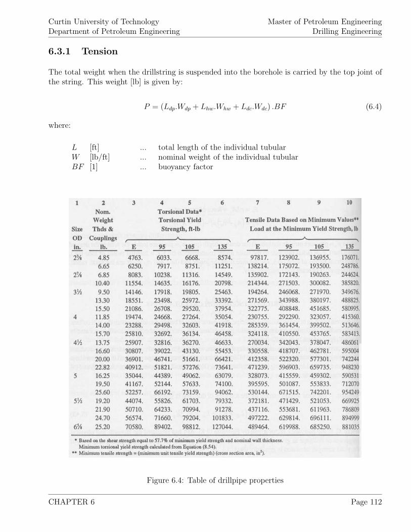
Curtin University of TechnologyDepartment of Petroleum Engineering
Master of Petroleum EngineeringDrilling Engineering
6.3.1 Tension
The total weight when the drillstring is suspended into the borehole is carried by the top joint ofthe string. This weight [lb] is given by:
P = (Ldp.Wdp + Lhw.Whw + Ldc.Wdc) .BF (6.4)
where:
L [ft] ... total length of the individual tubularW [lb/ft] ... nominal weight of the individual tubularBF [1] ... buoyancy factor
Figure 6.4: Table of drillpipe properties
CHAPTER 6 Page 112
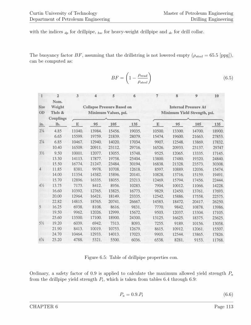
Curtin University of TechnologyDepartment of Petroleum Engineering
Master of Petroleum EngineeringDrilling Engineering
with the indices dp for drillpipe, hw for heavy-weight drillpipe and dc for drill collar.
The buoyancy factor BF , assuming that the drillstring is not lowered empty (ρsteel = 65.5 [ppg]),can be computed as:
BF =
(1 − ρmud
ρsteel
)(6.5)
Figure 6.5: Table of drillpipe properties con.
Ordinary, a safety factor of 0.9 is applied to calculate the maximum allowed yield strength Pa
from the drillpipe yield strength Pt, which is taken from tables 6.4 through 6.9:
Pa = 0.9.Pt (6.6)
CHAPTER 6 Page 113
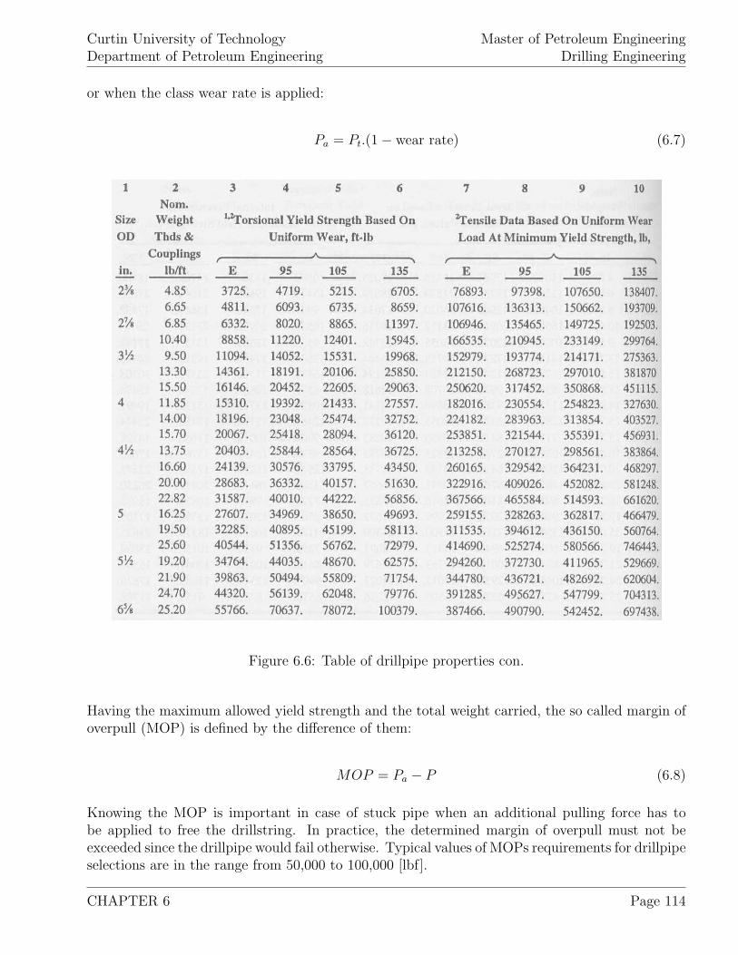
Curtin University of TechnologyDepartment of Petroleum Engineering
Master of Petroleum EngineeringDrilling Engineering
or when the class wear rate is applied:
Pa = Pt.(1 − wear rate) (6.7)
Figure 6.6: Table of drillpipe properties con.
Having the maximum allowed yield strength and the total weight carried, the so called margin ofoverpull (MOP) is defined by the difference of them:
MOP = Pa − P (6.8)
Knowing the MOP is important in case of stuck pipe when an additional pulling force has tobe applied to free the drillstring. In practice, the determined margin of overpull must not beexceeded since the drillpipe would fail otherwise. Typical values of MOPs requirements for drillpipeselections are in the range from 50,000 to 100,000 [lbf].
CHAPTER 6 Page 114
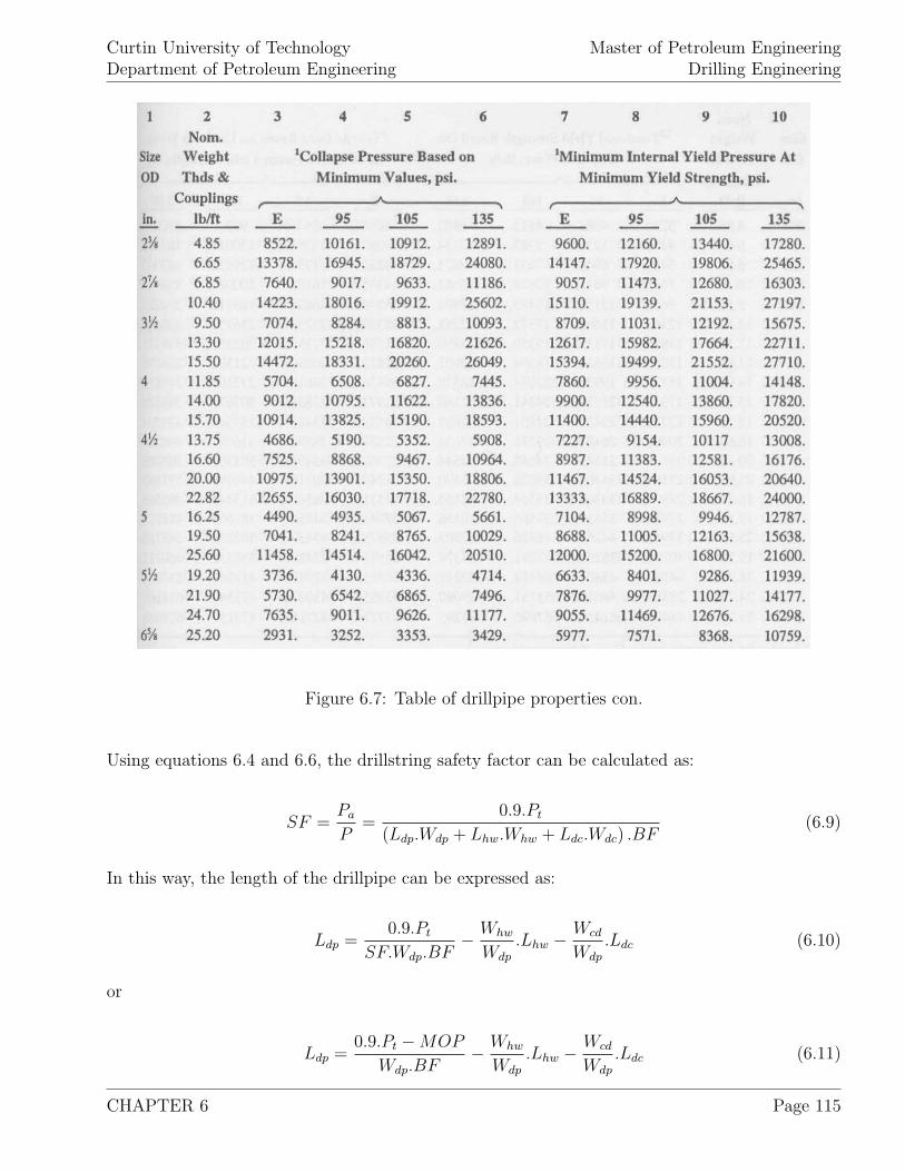
Curtin University of TechnologyDepartment of Petroleum Engineering
Master of Petroleum EngineeringDrilling Engineering
Figure 6.7: Table of drillpipe properties con.
Using equations 6.4 and 6.6, the drillstring safety factor can be calculated as:
SF =Pa
P=
0.9.Pt
(Ldp.Wdp + Lhw.Whw + Ldc.Wdc) .BF(6.9)
In this way, the length of the drillpipe can be expressed as:
Ldp =0.9.Pt
SF.Wdp.BF− Whw
Wdp
.Lhw − Wcd
Wdp
.Ldc (6.10)
or
Ldp =0.9.Pt − MOP
Wdp.BF− Whw
Wdp
.Lhw − Wcd
Wdp
.Ldc (6.11)
CHAPTER 6 Page 115
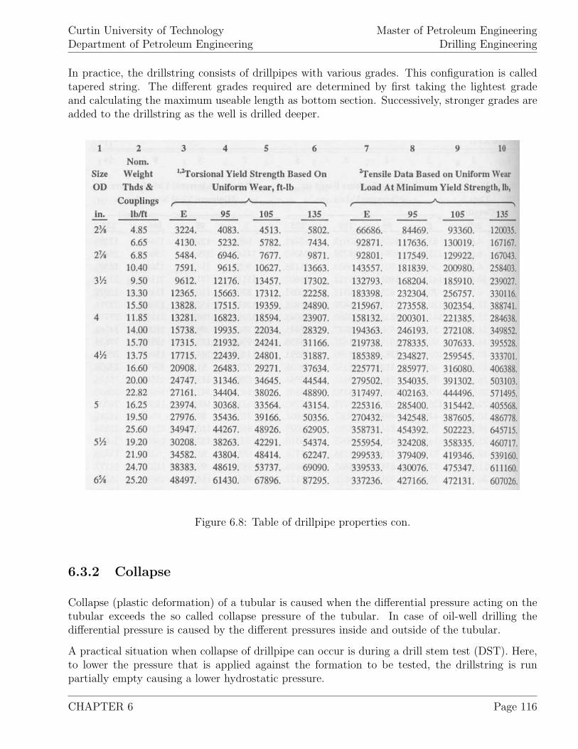
Curtin University of TechnologyDepartment of Petroleum Engineering
Master of Petroleum EngineeringDrilling Engineering
In practice, the drillstring consists of drillpipes with various grades. This configuration is calledtapered string. The different grades required are determined by first taking the lightest gradeand calculating the maximum useable length as bottom section. Successively, stronger grades areadded to the drillstring as the well is drilled deeper.
Figure 6.8: Table of drillpipe properties con.
6.3.2 Collapse
Collapse (plastic deformation) of a tubular is caused when the differential pressure acting on thetubular exceeds the so called collapse pressure of the tubular. In case of oil-well drilling thedifferential pressure is caused by the different pressures inside and outside of the tubular.
A practical situation when collapse of drillpipe can occur is during a drill stem test (DST). Here,to lower the pressure that is applied against the formation to be tested, the drillstring is runpartially empty causing a lower hydrostatic pressure.
CHAPTER 6 Page 116
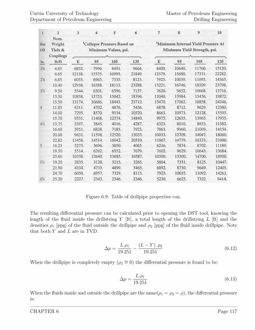
Curtin University of TechnologyDepartment of Petroleum Engineering
Master of Petroleum EngineeringDrilling Engineering
Figure 6.9: Table of drillpipe properties con.
The resulting differential pressure can be calculated prior to opening the DST tool, knowing thelength of the fluid inside the drillstring Y [ft], a total length of the drillstring L [ft] and thedensities ρ1 [ppg] of the fluid outside the drillpipe and ρ2 [ppg] of the fluid inside drillpipe. Notethat both Y and L are in TVD.
∆p =L.ρ1
19.251− (L − Y ) .ρ2
19.251(6.12)
When the drillpipe is completely empty (ρ2∼= 0) the differential pressure is found to be:
∆p =L.ρ1
19.251(6.13)
When the fluids inside and outside the drillpipe are the same(ρ1 = ρ2 = ρ), the differential pressureis:
CHAPTER 6 Page 117
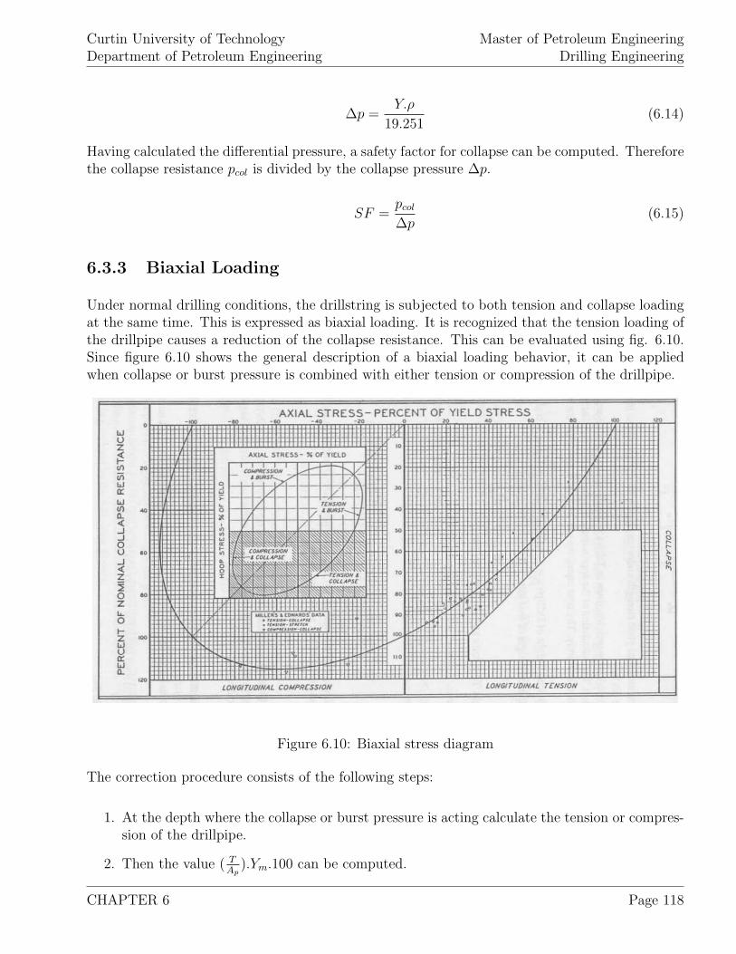
Curtin University of TechnologyDepartment of Petroleum Engineering
Master of Petroleum EngineeringDrilling Engineering
∆p =Y.ρ
19.251(6.14)
Having calculated the differential pressure, a safety factor for collapse can be computed. Thereforethe collapse resistance pcol is divided by the collapse pressure ∆p.
SF =pcol
∆p(6.15)
6.3.3 Biaxial Loading
Under normal drilling conditions, the drillstring is subjected to both tension and collapse loadingat the same time. This is expressed as biaxial loading. It is recognized that the tension loading ofthe drillpipe causes a reduction of the collapse resistance. This can be evaluated using fig. 6.10.Since figure 6.10 shows the general description of a biaxial loading behavior, it can be appliedwhen collapse or burst pressure is combined with either tension or compression of the drillpipe.
Figure 6.10: Biaxial stress diagram
The correction procedure consists of the following steps:
1. At the depth where the collapse or burst pressure is acting calculate the tension or compres-sion of the drillpipe.
2. Then the value ( TAp
).Ym.100 can be computed.
CHAPTER 6 Page 118
Curtin University of TechnologyDepartment of Petroleum Engineering
Master of Petroleum EngineeringDrilling Engineering
3. The fig. 6.10 is entered at the horizontal axis using above value.
4. Going vertically from this value, the ellipse curve is to be intersected
5. From this intersection, going horizontally to the vertical axis gives the value for Pca
Pco.100.
6. The adjusted pressure strength of the pipe is found with equation 6.16:.
Pca = Pco.Pca
Pco
(6.16)
where:
Pca [psi] ... adjusted collapse pressurePco [psi] ... simple collapse pressure
Instead of using fig. 6.10, the corrected collapse or burst resistance can be computed with:
Pca = Pco
√√√√1 − 0.75.
(TAp
Ym
)2
− 0.5.
TAp
Ym
(6.17)
6.3.4 Shock Loading
When the movement of the drillpipe is suddenly stopped (e.g. by setting slips), shock loadsdevelop that compromise an additional tensile force. This force is expressed as:
Fs = 3, 200.Wdp (6.18)
where:
Wdp [lbf/ft] ... weight of the drillpipe per unit lengthFs [lbf] ... shock loading force
6.3.5 Torsion
When making or breaking connections as well as when torques are applied during drilling opera-tions, the minimum torsional yield strength of the drillpipe must not be exceeded. The minimumtorsional yield strength of a tubular is calculated as:
CHAPTER 6 Page 119
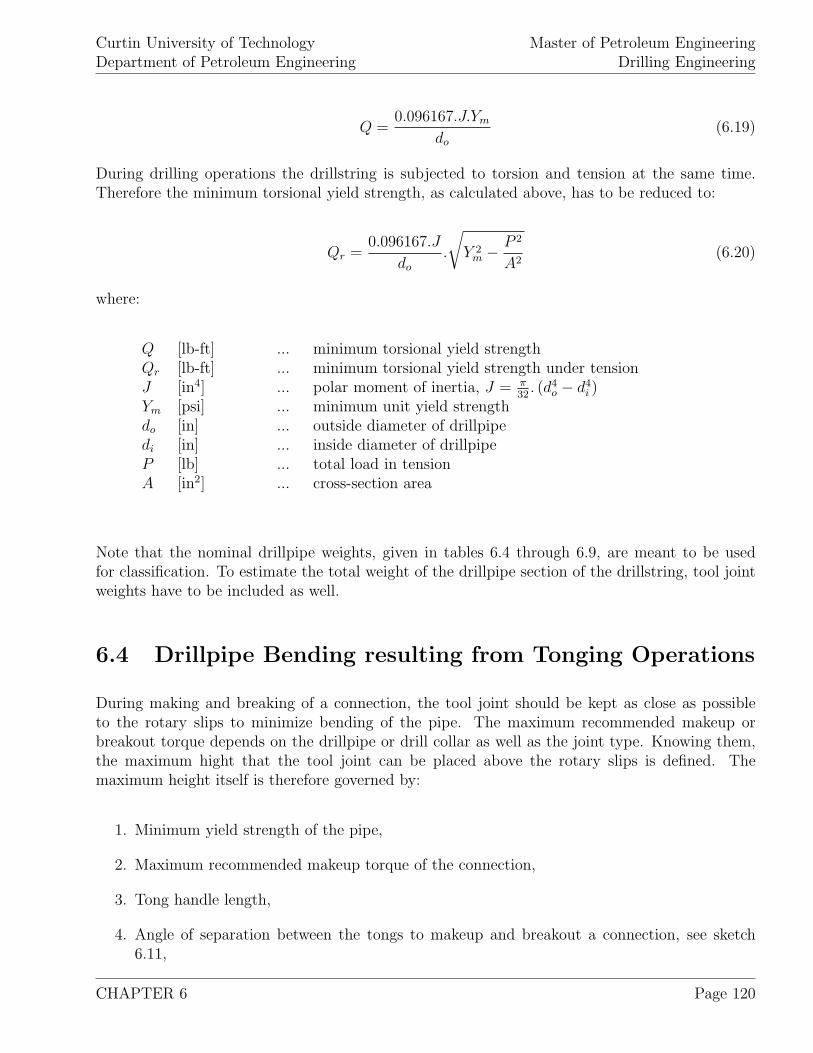
Curtin University of TechnologyDepartment of Petroleum Engineering
Master of Petroleum EngineeringDrilling Engineering
Q =0.096167.J.Ym
do
(6.19)
During drilling operations the drillstring is subjected to torsion and tension at the same time.Therefore the minimum torsional yield strength, as calculated above, has to be reduced to:
Qr =0.096167.J
do
.
√Y 2
m − P 2
A2(6.20)
where:
Q [lb-ft] ... minimum torsional yield strengthQr [lb-ft] ... minimum torsional yield strength under tensionJ [in4] ... polar moment of inertia, J = π
32. (d4
o − d4i )
Ym [psi] ... minimum unit yield strengthdo [in] ... outside diameter of drillpipedi [in] ... inside diameter of drillpipeP [lb] ... total load in tensionA [in2] ... cross-section area
Note that the nominal drillpipe weights, given in tables 6.4 through 6.9, are meant to be usedfor classification. To estimate the total weight of the drillpipe section of the drillstring, tool jointweights have to be included as well.
6.4 Drillpipe Bending resulting from Tonging Operations
During making and breaking of a connection, the tool joint should be kept as close as possibleto the rotary slips to minimize bending of the pipe. The maximum recommended makeup orbreakout torque depends on the drillpipe or drill collar as well as the joint type. Knowing them,the maximum hight that the tool joint can be placed above the rotary slips is defined. Themaximum height itself is therefore governed by:
1. Minimum yield strength of the pipe,
2. Maximum recommended makeup torque of the connection,
3. Tong handle length,
4. Angle of separation between the tongs to makeup and breakout a connection, see sketch6.11,
CHAPTER 6 Page 120
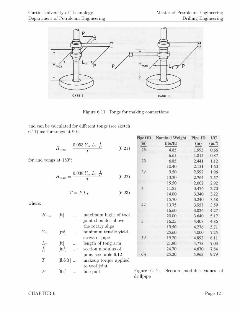
Curtin University of TechnologyDepartment of Petroleum Engineering
Master of Petroleum EngineeringDrilling Engineering
Figure 6.11: Tongs for making connections
Figure 6.12: Section modulus values ofdrillpipe
and can be calculated for different tongs (see sketch6.11) as: for tongs at 90◦:
Hmax =0.053.Ym.LT . I
C
T(6.21)
for and tongs at 180◦:
Hmax =0.038.Ym.LT . I
C
T(6.22)
T = P.LT (6.23)
where:
Hmax [ft] ... maximum hight of tooljoint shoulder abovethe rotary slips
Ym [psi] ... minimum tensile yieldstress of pipe
LT [ft] ... length of tong armIC
[in3] ... section modulus ofpipe, see table 6.12
T [lbf-ft] ... makeup torque appliedto tool joint
P [lbf] ... line pull
CHAPTER 6 Page 121
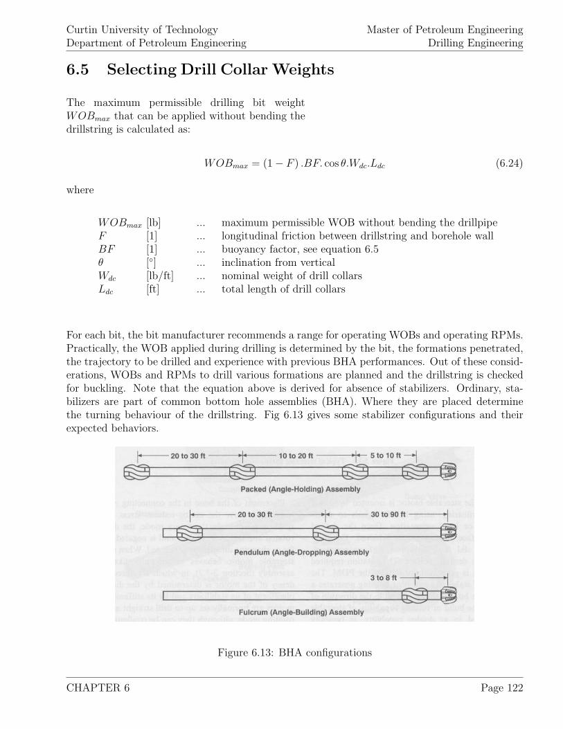
Curtin University of TechnologyDepartment of Petroleum Engineering
Master of Petroleum EngineeringDrilling Engineering
6.5 Selecting Drill Collar Weights
The maximum permissible drilling bit weightWOBmax that can be applied without bending thedrillstring is calculated as:
WOBmax = (1 − F ) .BF. cos θ.Wdc.Ldc (6.24)
where
WOBmax [lb] ... maximum permissible WOB without bending the drillpipeF [1] ... longitudinal friction between drillstring and borehole wallBF [1] ... buoyancy factor, see equation 6.5θ [◦] ... inclination from verticalWdc [lb/ft] ... nominal weight of drill collarsLdc [ft] ... total length of drill collars
For each bit, the bit manufacturer recommends a range for operating WOBs and operating RPMs.Practically, the WOB applied during drilling is determined by the bit, the formations penetrated,the trajectory to be drilled and experience with previous BHA performances. Out of these consid-erations, WOBs and RPMs to drill various formations are planned and the drillstring is checkedfor buckling. Note that the equation above is derived for absence of stabilizers. Ordinary, sta-bilizers are part of common bottom hole assemblies (BHA). Where they are placed determinethe turning behaviour of the drillstring. Fig 6.13 gives some stabilizer configurations and theirexpected behaviors.
Figure 6.13: BHA configurations
CHAPTER 6 Page 122
Curtin University of TechnologyDepartment of Petroleum Engineering
Master of Petroleum EngineeringDrilling Engineering
6.6 Stretch of Drillpipe
The elongation or stretch of the drillstring is caused by pulling the string as well as due to its ownweight. The amount of stretch itself depends on: the amount of pull, the length of the drillstring,the elasticity of the materials and the various cross-section areas. The elongations are found as:
due to weight carried:
e1 =P.L
735, 444.Wdp
(6.25)
due to its own weight:
e2 =L2
9.625.107. (65.44 − 1.44.ρm) (6.26)
where:
e1, e2 [in] ... drillstring stretchesP [lb] ... weight carriedWdp [lb/ft] ... weight of drillpipeρm [ppg] ... mud weightL [ft] ... length of drillpipe
To calculate the total stretch of the drillpipe, both stretches (e1 and e2) have to be added.
6.7 Critical Rotary Speeds
Rotating the drillstring at critical rotary speeds causes vibrations which lead to excessive wear,rapid deterioration, crooked drillpipe and fatigue failure.
In general, critical rotary speeds depend on length, seize and makeup of of the drillstring. Thecaused vibrations can be distinguished into:
1. Vibration in nodes. Here the pipe between each joint vibrates.
2. Vibration of the total drillstring. Here the vibration is classified as a spring pendulum one.
Equation 6.27 calculates the critical rotation speed for vibration type 1:
RPM =4, 760, 000
l2.√
d2o − d2
i (6.27)
CHAPTER 6 Page 123
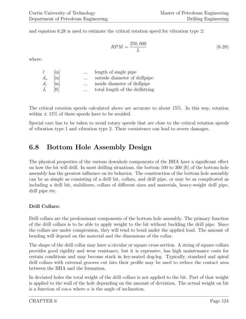
Curtin University of TechnologyDepartment of Petroleum Engineering
Master of Petroleum EngineeringDrilling Engineering
and equation 6.28 is used to estimate the critical rotation speed for vibration type 2:
RPM =258, 000
L(6.28)
where:
l [in] ... length of single pipedo [in] ... outside diameter of drillpipedi [in] ... inside diameter of drillpipeL [ft] ... total length of the drillstring
The critical rotation speeds calculated above are accurate to about 15%. In this way, rotationwithin ± 15% of these speeds have to be avoided.
Special care has to be taken to avoid rotary speeds that are close to the critical rotation speedsof vibration type 1 and vibration type 2. Their coexistence can lead to severe damages.
6.8 Bottom Hole Assembly Design
The physical properties of the various downhole components of the BHA have a significant effecton how the bit will drill. In most drilling situations, the bottom 100 to 300 [ft] of the bottom holeassembly has the greatest influence on its behavior. The construction of the bottom hole assemblycan be as simple as consisting of a drill bit, collars, and drill pipe, or may be as complicated asincluding a drill bit, stabilizers, collars of different sizes and materials, heavy-weight drill pipe,drill pipe etc.
Drill Collars:
Drill collars are the predominant components of the bottom hole assembly. The primary functionof the drill collars is to be able to apply weight to the bit without buckling the drill pipe. Sincethe collars are under compression, they will tend to bend under the applied load. The amount ofbending will depend on the material and the dimensions of the collar.
The shape of the drill collar may have a circular or square cross section. A string of square collarsprovides good rigidity and wear resistance, but it is expensive, has high maintenance costs forcertain conditions and may become stuck in key-seated dog-leg. Typically, standard and spiraldrill collars with external grooves cut into their profile may be used to reduce the contact areabetween the BHA and the formation.
In deviated holes the total weight of the drill collars is not applied to the bit. Part of that weightis applied to the wall of the hole depending on the amount of deviation. The actual weight on bitis a function of cos α where α is the angle of inclination.
CHAPTER 6 Page 124
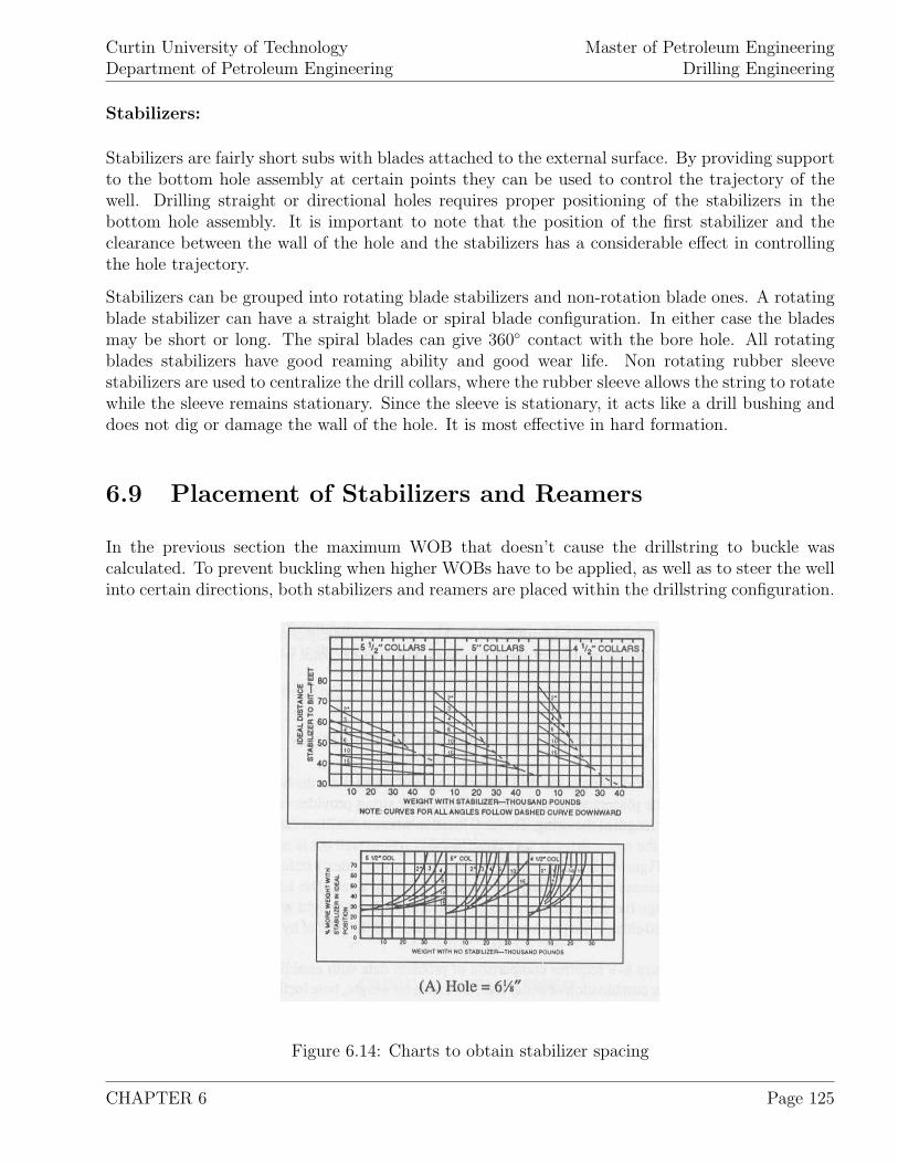
Curtin University of TechnologyDepartment of Petroleum Engineering
Master of Petroleum EngineeringDrilling Engineering
Stabilizers:
Stabilizers are fairly short subs with blades attached to the external surface. By providing supportto the bottom hole assembly at certain points they can be used to control the trajectory of thewell. Drilling straight or directional holes requires proper positioning of the stabilizers in thebottom hole assembly. It is important to note that the position of the first stabilizer and theclearance between the wall of the hole and the stabilizers has a considerable effect in controllingthe hole trajectory.
Stabilizers can be grouped into rotating blade stabilizers and non-rotation blade ones. A rotatingblade stabilizer can have a straight blade or spiral blade configuration. In either case the bladesmay be short or long. The spiral blades can give 360◦ contact with the bore hole. All rotatingblades stabilizers have good reaming ability and good wear life. Non rotating rubber sleevestabilizers are used to centralize the drill collars, where the rubber sleeve allows the string to rotatewhile the sleeve remains stationary. Since the sleeve is stationary, it acts like a drill bushing anddoes not dig or damage the wall of the hole. It is most effective in hard formation.
6.9 Placement of Stabilizers and Reamers
In the previous section the maximum WOB that doesn’t cause the drillstring to buckle wascalculated. To prevent buckling when higher WOBs have to be applied, as well as to steer the wellinto certain directions, both stabilizers and reamers are placed within the drillstring configuration.
Figure 6.14: Charts to obtain stabilizer spacing
CHAPTER 6 Page 125
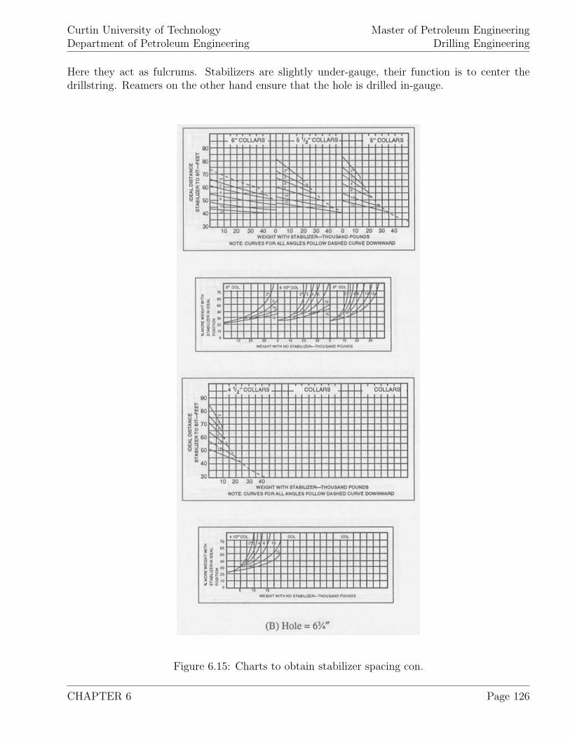
Curtin University of TechnologyDepartment of Petroleum Engineering
Master of Petroleum EngineeringDrilling Engineering
Here they act as fulcrums. Stabilizers are slightly under-gauge, their function is to center thedrillstring. Reamers on the other hand ensure that the hole is drilled in-gauge.
Figure 6.15: Charts to obtain stabilizer spacing con.
CHAPTER 6 Page 126
Curtin University of TechnologyDepartment of Petroleum Engineering
Master of Petroleum EngineeringDrilling Engineering
Figure 6.16: Charts to obtain stabilizer spacing con.
CHAPTER 6 Page 127
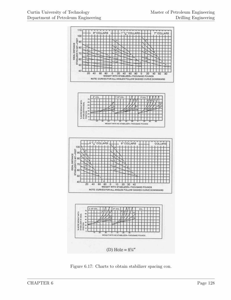
Curtin University of TechnologyDepartment of Petroleum Engineering
Master of Petroleum EngineeringDrilling Engineering
Figure 6.17: Charts to obtain stabilizer spacing con.
CHAPTER 6 Page 128
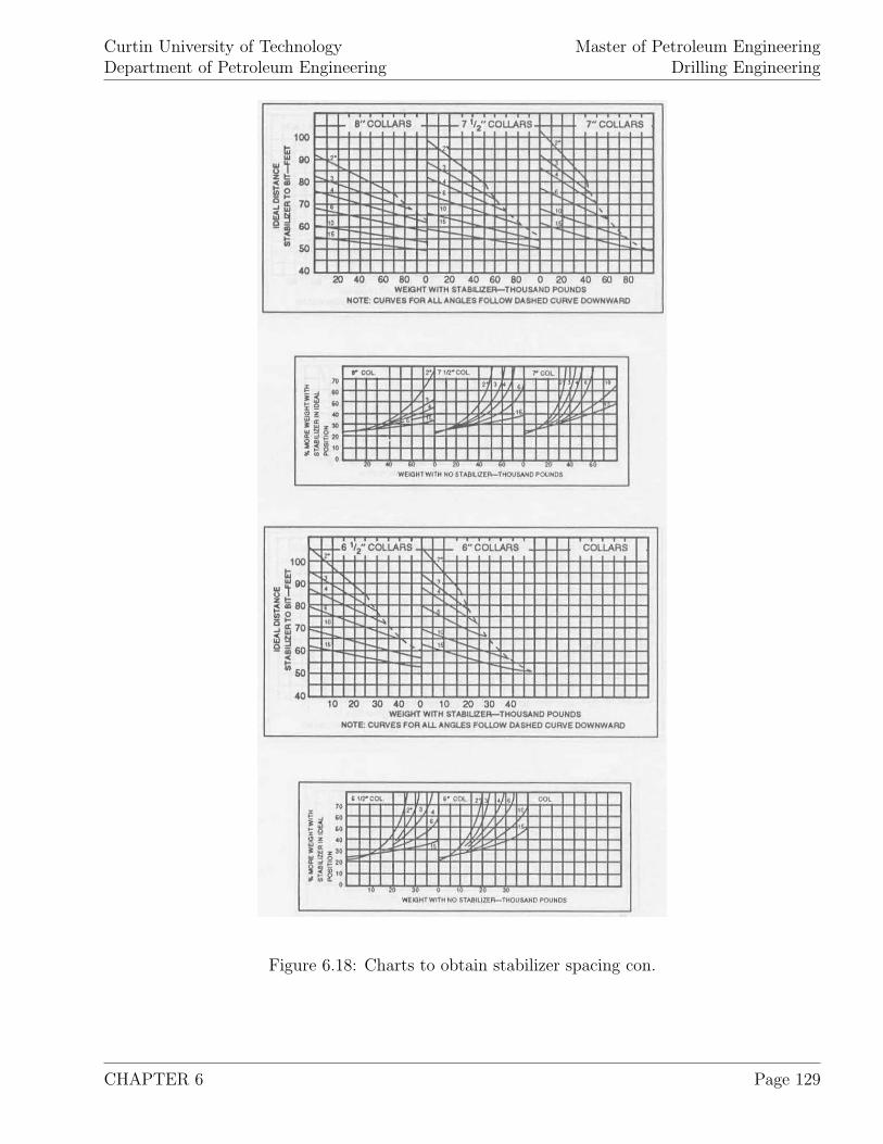
Curtin University of TechnologyDepartment of Petroleum Engineering
Master of Petroleum EngineeringDrilling Engineering
Figure 6.18: Charts to obtain stabilizer spacing con.
CHAPTER 6 Page 129
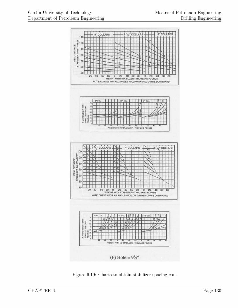
Curtin University of TechnologyDepartment of Petroleum Engineering
Master of Petroleum EngineeringDrilling Engineering
Figure 6.19: Charts to obtain stabilizer spacing con.
CHAPTER 6 Page 130
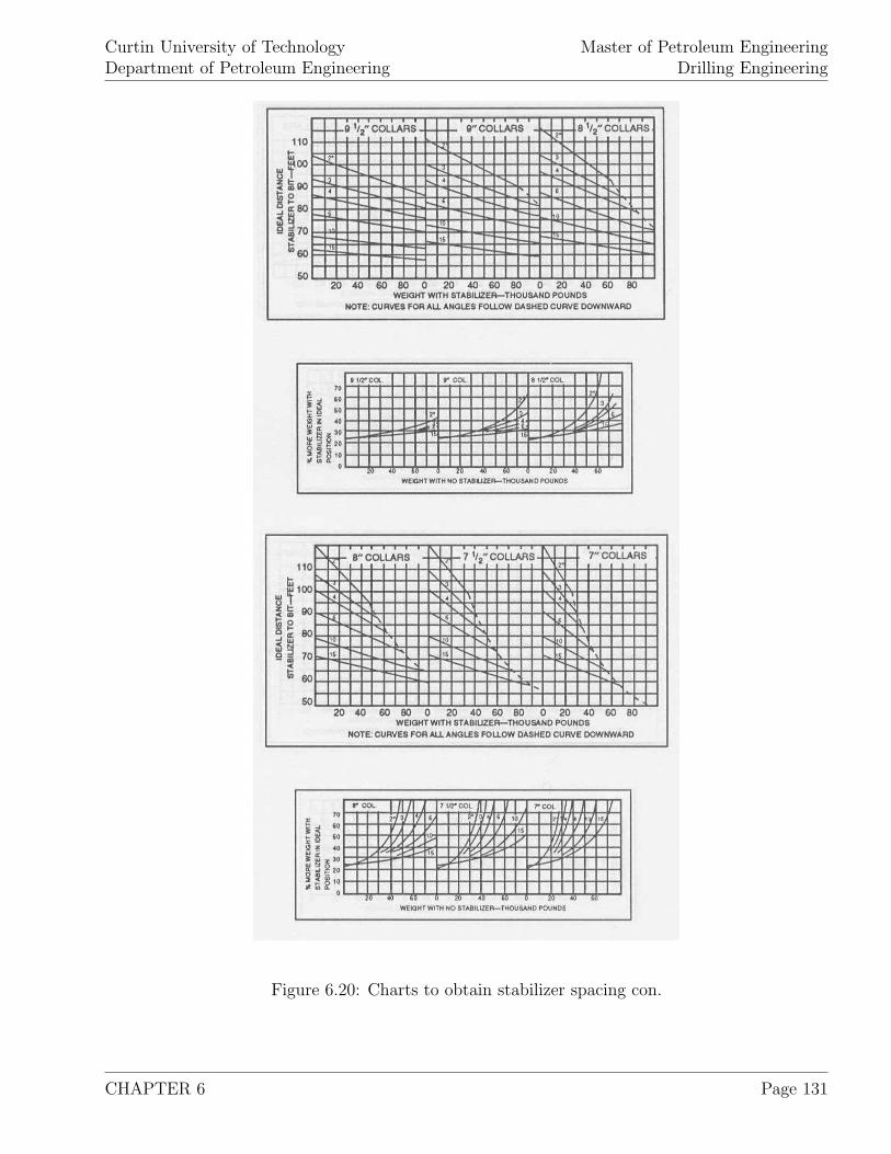
Curtin University of TechnologyDepartment of Petroleum Engineering
Master of Petroleum EngineeringDrilling Engineering
Figure 6.20: Charts to obtain stabilizer spacing con.
CHAPTER 6 Page 131
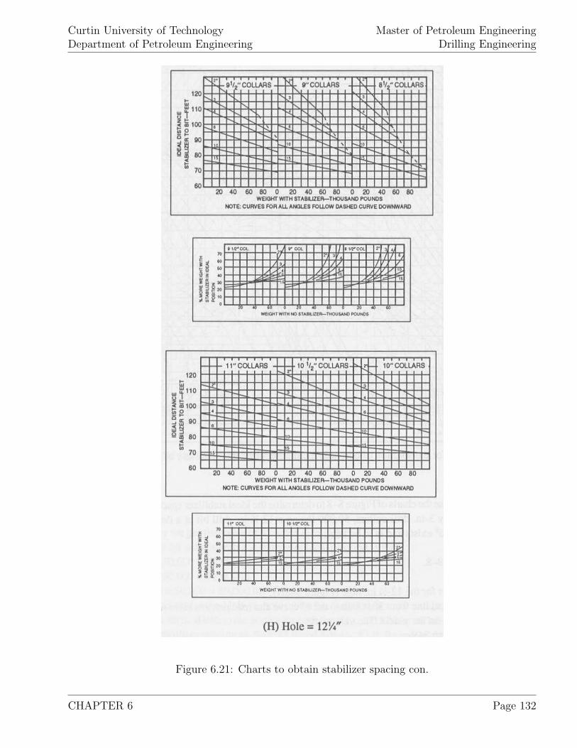
Curtin University of TechnologyDepartment of Petroleum Engineering
Master of Petroleum EngineeringDrilling Engineering
Figure 6.21: Charts to obtain stabilizer spacing con.
CHAPTER 6 Page 132
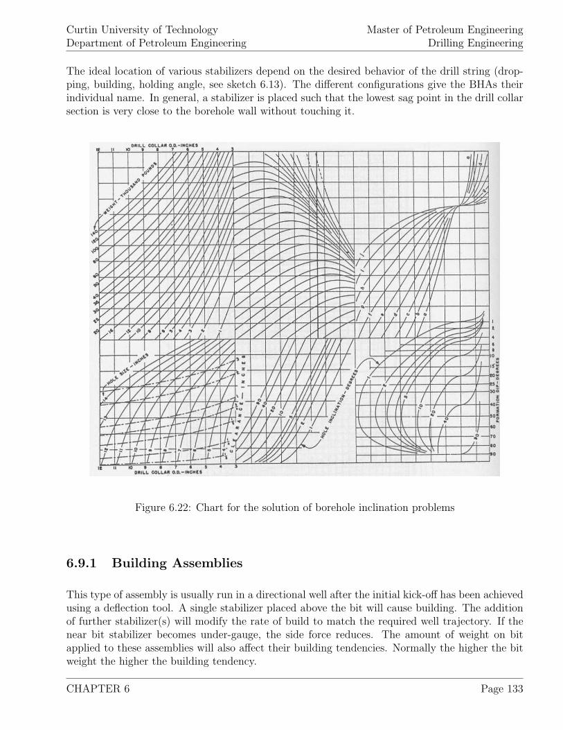
Curtin University of TechnologyDepartment of Petroleum Engineering
Master of Petroleum EngineeringDrilling Engineering
The ideal location of various stabilizers depend on the desired behavior of the drill string (drop-ping, building, holding angle, see sketch 6.13). The different configurations give the BHAs theirindividual name. In general, a stabilizer is placed such that the lowest sag point in the drill collarsection is very close to the borehole wall without touching it.
Figure 6.22: Chart for the solution of borehole inclination problems
6.9.1 Building Assemblies
This type of assembly is usually run in a directional well after the initial kick-off has been achievedusing a deflection tool. A single stabilizer placed above the bit will cause building. The additionof further stabilizer(s) will modify the rate of build to match the required well trajectory. If thenear bit stabilizer becomes under-gauge, the side force reduces. The amount of weight on bitapplied to these assemblies will also affect their building tendencies. Normally the higher the bitweight the higher the building tendency.
CHAPTER 6 Page 133
Curtin University of TechnologyDepartment of Petroleum Engineering
Master of Petroleum EngineeringDrilling Engineering
6.9.2 Holding Assemblies
Once the inclination has been built to the required angle, the tangential section of the well isdrilled using a holding assembly. Holding assemblies do not maintain inclination angle; rather,they minimize angle build or drop.
Minimal tilt angle at the bit, as well as stiffness of the bottom hole assembly near the bit helpsmaintain inclination angle. Change in weight on bit does not affect the directional behavior of thistype of assembly and so optimum weight on bit can be applied to achieve maximum penetrationrates.
6.9.3 Dropping Assemblies
The application of a dropping assembly is that when the inclination has been increased beyondthe intending trajectory and must be reduced to bring the well back on course. Normally theseBHA configurations are more effective in high angled holes. If the hole angle does not decrease,the weight on bit can be reduced with use of these assemblies, although this will also reduce thepenetration rate.
6.9.4 WOB Increase
Since stabilizers reduce the drillstring tendency to buckle, larger WOBs can be applied. It iscommon to express the possible increase in WOB as a percentage of the maximum allowed WOBwithout stabilizers. For commonly encountered borehole seizes figure 6.13 can be applied toderive the proper position of a stabilizer and the resulting bit weight increase when the maximumallowable WOB without stabilizer is known. This figure is also applied to compare the data toplan for with practically established data using other combinations of drill collar seize, bit weight,borehole seize, borehole inclination and formation dip.
In practice, since the ideal position of the stabilizer is based on a particular scenario and the BHAsare not always changed when the trajectory of the well changes, a compromise when designing theBHA has to be formed. Therefore the stabilizer is placed between the ideal position, as derivedabove and about 10% closer to the bit. When very light weight on bit is run (nonpacked holes),the stabilizer position should not be closer than 5% to the bit than the ideal position, as it iscalculated above.
6.10 Dogleg Severity Analysis
Dogleg severity is defined as total curvature of the wellbore per 100 [ft] and is expressed with theunit [◦/100 ft].
Most of drillpipe failure is caused by fatigue wear, which occurs due to of cycle bending stressesand axial stresses when the drillpipe under load rotates along a sharp bend (dogleg).
CHAPTER 6 Page 134
Curtin University of TechnologyDepartment of Petroleum Engineering
Master of Petroleum EngineeringDrilling Engineering
Since the drilling fatigue is based on the combination of bending and axial stresses as well astension in the drillpipe, fatigue danger is highest in the upmost part of the drillstring. Thereforeshallow, sharp bends of the trajectory of deep wells are to be avoided. In these situations rotationoff bottom (no WOB) increases the danger of fatigue wear since the weight of the drill collarsincrease the tension load.
To calculate the maximum permissible dogleg severity, equations 6.31 is used:
I =π
64.(d4
o − d4i
)(6.29)
K =
√T
E.I(6.30)
C =432, 000
π.
σb
E.D.tanh (K.L)
K.L(6.31)
where:
C [◦/100 ft] ... maximum permissible dogleg severityT [lb] ... buoyant weight suspended below the dogleg
(including tool joints)E [psi] ... Young’s modulus (steel: E = 30.106 [psi])I [in4] ... drillpipe moment of inertiado [in] ... drillpipe outside diameterdi [in] ... drillpipe inside diameterσb [psi] ... maximum permissible bending stressD [in] ... drillpipe outer diameterL [in] ... half the distance between tool joints
(for range 2 drillpipe: 180 [in])
Using the buoyant tensile stress σt [psi], the maximum permissible bending stress σb [psi] can befound for different grades of drillpipe.
σt =T
A(6.32)
Grade E75 drillpipe:
σb = 19, 500 − 10
67.σt − 0.6
6702. (σt − 33, 500)2 (6.33)
Grade S135 drillpipe:
CHAPTER 6 Page 135
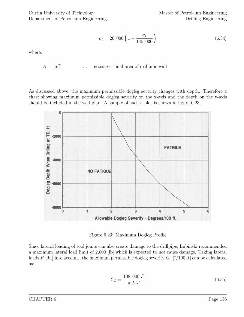
Curtin University of TechnologyDepartment of Petroleum Engineering
Master of Petroleum EngineeringDrilling Engineering
σb = 20, 000
(1 − σt
145, 000
)(6.34)
where:
A [in2] ... cross-sectional area of drillpipe wall
As discussed above, the maximum permissible dogleg severity changes with depth. Therefore achart showing maximum permissible dogleg severity on the x-axis and the depth on the y-axisshould be included in the well plan. A sample of such a plot is shown in figure 6.23.
Figure 6.23: Maximum Dogleg Profile
Since lateral loading of tool joints can also create damage to the drillpipe, Lubinski recommendeda maximum lateral load limit of 2,000 [lb] which is expected to not cause damage. Taking lateralloads F [lbf] into account, the maximum permissible dogleg severity CL [◦/100 ft] can be calculatedas:
CL =108, 000.F
π.L.T(6.35)
CHAPTER 6 Page 136

Curtin University of TechnologyDepartment of Petroleum Engineering
Master of Petroleum EngineeringDrilling Engineering
6.11 Examples
1. To drill a well to a depth of 13,500 [ft] using a 5 [in], 19.5 [lb/ft], 4.276 [in] ID grade E and gradeX95 new drillpipe. The total length and weight of the drill collars and heavy-weight drillpipe are984 [ft] and 157,374 [lb] respectively. The maximum expected mud weight at 12,000 [ft] is 12.5[ppg]. Calculate the:
(a) Maximum length of each grade of drillpipe that can be usedif a MOP of 50,000 [lb] is to be maintained for the lower grade,
(b) MOP of the heavier grade.
2. A WOB of 50,000 [lb] is to be put on a 12-14
[in] bit at a depth of 10,000 [ft]. As assemble, 8[in] OD, 3 [in] ID, 147 [lb/ft] drill collars are connected to 5 [in], 19.5 [lb/ft] drillpipe. The appliedmud weight is 12.5 [ppg]. What is the required length of drill collars to drill a:
(a) Vertical hole,(b) Deviated hole with θ = 45◦
3. To run a 4.5 [in] OD liner weighting 50,000 [lb] to 10,000 [ft], a 5 [in] drillpipe, 19.5 [lb/ft],grade E premium class is used. What is the total stretch of the 8,500 [ft] long drillpipe when themud weight is 12.5 [ppg]?
4. Determine the bit weight of the problem data when:
Established data: 7 [in] drill collar OD, 40,000 [lb] WOB, 9 [in] hole seize, 10◦ inclination;
Problem data: 11 [in] drill collar OD, 12 [in] hole seize, 10◦ inclination.
5. What is the ideal stabilizer spacing and percent more bit weight for 8 [in] OD, 3 [in] IDdrill collars when 50,000 [lb] WOB shall be applied on a 12-1
4bit at a depth of 10,000 [ft]? The
equilibrium angle exists and is kept at 6◦.
6. A 10,000 [ft] drillstring consists of 9,700 [ft] 5 [in] OD, 4.276 [in] ID, 19.5 [lb/ft], premiumgrade E drillpipe and 300 [ft] of 8 [in] OD, 3 [in] ID, 147 [lb/ft] drill collars. The used drillingmud weight is 12.5 [ppg] and the applied WOB is 45,000 [lb]. What is the maximum permissibledogleg severity of the drillpipe at 3,000 [ft]?
CHAPTER 6 Page 137

Curtin University of TechnologyDepartment of Petroleum Engineering
Master of Petroleum EngineeringDrilling Engineering
7. A drillstring has to be designed using grade E, G and S, premium pipes with OD 5 [in], ID4.276 [in]. The drill collar used is OD 7 [in], ID 2.5 [in], mud weight applied is 15 [ppg]. Whena minimum of 100,000 [lb] MOP is required, how deep can be drilled? What is the MOP whendrilling at 25,000 [ft]?
CHAPTER 6 Page 138
Curtin University of TechnologyDepartment of Petroleum Engineering
Master of Petroleum EngineeringDrilling Engineering
Chapter 7
Drilling Fluid
Drilling fluid or also called drilling mud is a mixture of water, oil, clay and various chemicals.Within drilling it performs various functions and contributes with a large portion to the total wellcosts. In this way the mud system (or mud program) has to be carefully designed to ensure asuccessful drilling project.
7.1 Functions of Drilling Mud
As mentioned above, the drilling mud serves many purposes which may not all be achieved simul-taneously for all parts of the well. In this way an individual prioritizing has to followed. Below isa summery of some main mud functions:
1. The mud has to transport the drilling cuttings from the bottom of the hole to the surface.For this, a high mud circulation velocity, a high mud density and a high mud viscosity arefavorable.
2. Once the cuttings are at the surface, efficient mud cleaning (separation of cuttings, formationgas, etc. from the mud) has to be possible applying a reasonable amount of cleaning equip-ment. For further circulation, mud pumps allow ordinary a maximum of 2% sand contentwithout showing excessive wear.
3. The mud has to cool and lubricate the drilling bit as well as the drilling string to minimizeits wear. Adding of bentonite, oil and various emulsifying agents as well as graphite favorsthe cooling capability.
4. At overbalanced drilling, the mud has to seal off permeable formations by forming an im-permeable, relatively thin mud cake at the borehole wall of the permeable formations. Thiscapability can be obtained by adding of bentonite and chemical treatment of the mud whichenhances deflocculation and solids distribution.
CHAPTER 7 Page 139
Curtin University of TechnologyDepartment of Petroleum Engineering
Master of Petroleum EngineeringDrilling Engineering
5. Commonly, the mud has to create an overbalanced drilling condition to control the formationpressure. Mud weight is increased with additives like barite to create a hydrostatic pressureinside the well which is slightly higher than the formation pressure. Normally, an overbalanceof 100 to 200 [psi] has proven to be adequate to establish safe drilling.
6. Capability to hold drilling cuttings in suspension when circulation is interrupted. Failure ofthis capability would allow the cuttings to move down the hole, settle at favorable placesand block the drillstring. This thixotropic capability depends on the individual gel strengthof the drilling mud.
7. To create a buoyance force to partly support the weight of the drillstring and casing string.The buoyance force is strongly depended on the mud weight used. An increase in mud weightthat increases the buoyance results in smaller surface equipment requirements.
8. Reduce formation damage of various horizons penetrated. The borehole should be drilledin-gauge (borehole seize = drill bit seize) and either cave-ins (logging and stuck pipe) or wash-outs (possible cementing problems) avoided. Also the invasion of mud and small cuttingsinto the formation or chemical reaction of the mud with the formation have to be avoidedsince these would induce a positive skin effect and reduce later production rates.
9. The drilling mud should be neural to the proposed logs run and thus allow to obtain accurateinformation about the formations penetrated.
10. The drilling fluid has to transmit the hydraulic horsepower to the bit and allow maximumpenetration rates.
11. The mud system should minimize the torque and drag of the drillstring to decrease wearand possible failure as well as stuck pipe.
12. For the usage of while drilling tools, the mud should be able to carry the measurement signal(e.g. as mud pulses).
7.2 Types of Drilling Mud
Out of these different functions, the composition of a particular mud system does depend onthe actual requirements of the individual well or well section. Wells are drilled through differentformations that require different mud properties to achieve optimum penetrations and stableborehole conditions. Therefore economics, component and additives availability, temperature andcontamination are just a few of the major factors that determine the design of a particular mudprogram.
All the possible mixtures that form drilling mud can be generally characterised by the followingsystem. Further sub-classifications do exist.
CHAPTER 7 Page 140
Curtin University of TechnologyDepartment of Petroleum Engineering
Master of Petroleum EngineeringDrilling Engineering
1. Water based muds
(a) Clear water and native mud
(b) Inhibitive water-based mud – calcium muds
(c) Dispersed muds – lignosulphonate muds
(d) Nondispersed muds – KCL/polymer muds
(e) Flocculated muds
(f) Salt-saturated muds
2. Oil-base muds
3. Emulsion muds
(a) Oil-in-water emulsions
(b) Water-in-oil emulsions
4. Aerated muds
(a) Air
(b) Natural gas
(c) Mist, foam, or aerated muds
7.2.1 Water-base Muds
The term water-base mud refers to any drilling fluid where the continuous phase, in which somematerials are in suspension and others are dissolved, is water. Thus any water-base mud systemconsists of a water phase, inert solids, a reactive solids phase and chemical additives. Each ofthese parts contribute to the overall mud properties. The individual contributions are:
water: create initial viscosity.
inert solids (low-gravity solids like sand and chert and high-gravity solids likebarite and lead sulfides): produce required mud weight.
reactive solids (low-gravity solids like bentonite and attapulgite clays):cause further viscosity and yield point.
chemical additives (mud thinners like phosphate, chrome, lignosulphonate, lignites,and surfactants, and mud thickeners like lime, cement andpolymers): aid to control viscosity, yield point, gel strength,fluid loss, pH-value, filtration behavior.
CHAPTER 7 Page 141
Curtin University of TechnologyDepartment of Petroleum Engineering
Master of Petroleum EngineeringDrilling Engineering
To control corrosion, hydrogen embrittlement and the solubility of Ca2+ and Mg2+, a high pHvalue is required and can be controlled with caustic (NaOH).
Clear Water and Native Muds
To drill compact formations which are normally pressured (formation pressure equals hydrostaticpressure caused by formation fluids), fresh water and salt-saturated water can be used as drillingmud. As the name indicates, native muds are a mixture of water and clays or shales from thecuttings drilled. Here the clays or shales are dissolved by the water and returned to the surface.Clear water and native muds are the cheapest mud systems since no additional material to formthe mud is needed. They are also environmentally best accepted.
Inhibitive water-base Mud – Calcium Muds
When swelling and hydration of clays and shales are expected, inhibitive water-base muds can beapplied. Calcium muds are best suited to penetrate horizons that contain gypsum and hydrite. Asubclassification of inhibitive water-base muds distinguishes seawater muds, saturated saltwatermuds, lime muds and gypsum muds.
Dispersed Muds – Lignosulphonate Muds
Dispersed muds are used when the mud has to have following characteristics: relative high mudweight (larger than 14 [ppg]), used at moderately high formation temperatures, low filtration lossrequired and high tolerance for contamination by drilling solids.
Some of the disadvantages when using dispersed muds are: heaving of shales and causing formationdamage due to dispersant of formation clays in the presence of lignosulphonate.
Dispersed mud systems consist of: fresh or salty water, bentonite, lignosulphonate, caustic sodaand colloidal polymers (carboxy methyl cellulose or stabilized starch). In general, these mudsystems exhibit better control of viscosity, a higher solids tolerance and a better control of filtrationthan nondispersed muds.
Nondispersed Muds – KCL/Polymer Muds
To drill water sensitive and sloughing shales such as productive sands which are prone to formationdamage, fresh water nondispersed muds are applied. Commonly, nondispersed muds are associatedwith low mud weights and low solid concentrations.
Nondispersed mud systems consist of: fresh water or brine, potassium chloride (KCl), inhibitingpolymer, viscosifier, stabilized starch or carboxy methyl cellulose, caustic soda and lubricants.
CHAPTER 7 Page 142
Curtin University of TechnologyDepartment of Petroleum Engineering
Master of Petroleum EngineeringDrilling Engineering
Low-solids polymer mud systems are widespread in the industry since they offer advantages likeincreased penetration rate, hole stability, shear thinning ability, hole cleaning with maximumhydraulics and lower equivalent circulation density over conventional deflocculated muds. Withall these advantages, they also have disadvantages like instability at temperatures above 250 [F],irreversible absorption of the polymer on clay, a higher dilution and an adequate solids removalequipment is required as well as they are more corrosive.
Flocculated Muds
Flocculated muds posses generally a dynamic increase in filtration, viscosity and gel strength.Flocculation refers to a thickening of the mud due to edge-to-edge and edge-to-face associationof clay particles. The flocculation is commonly caused by high active solids concentration, highelectrolyte concentration and high temperature. To reduce the flocculating tendency of the mud,chemical additives, also called deflocculants or thinners are used. Thinners like phosphates, tan-nins, lignins and lignosulphonate are applied to lower the yield point and gel strength. Whendeflocculants are added, the pH-value is controlled by NaOH.
Salt-saturated Muds
Salt-saturated muds are used to drill through salt domes and salt sections. These mud systems aresaturated with sodium chloride (NaCL) that prevents severe hole enlargements due to washoutsof the salt formations. Swelling of bentonitic shales is controlled by adding of polymer.
7.2.2 Oil-base Muds
Opposite to water-base muds where water is the continuous phase, at oil-base mud systems crudeor diesel oil forms the continuous phase in the water-in-oil emulsion. In this way oil-base mud canhave as little as 3% to 5% or as much as 20% to 40% (invert emulsions) water content. Oil-basemud systems are applied when:
1. Drilling sensitive production zones or problem shales,
2. Drilling salt sections and formations that contain hydrogen sulfide,
3. Danger of stuck pipe problems,
4. Drilling at bottom hole temperatures that are permissable by water-base muds.
Low-gravity solids content has to be monitored closely when drilling with oil-base muds sinceat this environment solids do not hydrate which causes low-gravity solids contents to exceedacceptable levels often. This results in reduction of penetration rate, formation damage andincrease in risk of differential sticking.
CHAPTER 7 Page 143
Curtin University of TechnologyDepartment of Petroleum Engineering
Master of Petroleum EngineeringDrilling Engineering
Since oil-base muds contain substantially less colloidal particles, they exhibit a spurt fluid loss.Due to the higher filtration rates, the monitoring of high-pressure high-temperature filtration aswell as the drilling conditions are important to ensure that excessive filtration or filter cake buildupdoes not lead to problems.
7.3 Mud Calculations
The fundamental properties to describe a drilling mud are:
1. Mud weight,
2. Plastic viscosity,
3. Yield point,
4. Gel strength,
5. Filtrate and filter cake,
6. pH-value.
The procedures and equations to calculate the rheological properties like the plastic viscosity, theyield point and the gel strength were discussed at drilling hydraulics. In the following, the reamingmud characteristics and their measurement in the field are elaborated.
pH Determination
The pH-vale is defined as negative logarithm of the hydrogen ion content of a solution (pH =− log[H+]). In this way, an increase of the concentration of H+ ions decreases the pH-value and adecrease of H+ ions increases the pH-value. When the pH-value is known, it is determined whetherthe mud is acidic (OH− < H+ thus pH-value < 7) or alkaline (OH− > H+, thus pH-value > 7). ApH-value of 7 indicates a neutral mud.
Measuring the pH-value of a fluid is either performed with the help of a pH-meter or a specialpH-paper which changes color according to the pH-value determined.
The OH− concentration within a solution, at a given pH-value, is defined by:
[H+] [
OH−] = 1.0.10−4 (7.1)
or:
[OH−] = 10(pH−14) (7.2)
CHAPTER 7 Page 144
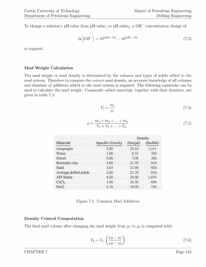
Curtin University of TechnologyDepartment of Petroleum Engineering
Master of Petroleum EngineeringDrilling Engineering
To change a solution’s pH-value from pH-value1 to pH-value2, a OH− concentration change of
∆[OH−] = 10(pH2−14) − 10(pH1−14) (7.3)
is required.
Mud Weight Calculation
The mud weight or mud density is determined by the volumes and types of solids added to themud system. Therefore to compute the correct mud density, an accurate knowledge of all volumesand densities of additives added to the mud system is required. The following equations can beused to calculate the mud weight. Commonly added materials, together with their densities, aregiven in table 7.1.
Vi =mi
ρi
(7.4)
ρ =m1 + m2 + ... + mn
V1 + V2 + ... + Vn
(7.5)
Figure 7.1: Common Mud Additives
Density Control Computation
The final mud volume after changing the mud weight from ρ1 to ρ2 is computed with:
V2 = V1.
(ρB − ρ1
ρB − ρ2
)(7.6)
CHAPTER 7 Page 145
Curtin University of TechnologyDepartment of Petroleum Engineering
Master of Petroleum EngineeringDrilling Engineering
In practice, since excess storage capacity is not available and to limit the amount of added, costlyweighting material, before the density is increase (e.g. by adding barite), some mud volume isdiscarded from the circulation system. In this situation, equation 7.7 calculates the volume theexisting mud has to be reduced to before weighting material is added:
V1 = V2.
(ρB − ρ2
ρB − ρ1
)(7.7)
With the knowledge of the volumes, the densities of the original mud and the weighting material,the weight of barite required is given by:
mB = 42. (V2 − V1) .ρB (7.8)
where:
mB [lbm] ... weight of API bariteρB [ppg] ... density of API bariteρ1 [ppg] ... density of original mud before weightingρ2 [ppg] ... density of final mud after weightingV1 [bbl] ... volume of original mud before weightingV2 [bbl] ... volume of final mud after weighting
Due to the barite’s extremely large surface area, barite has the tendency to adsorb a large amountof water from the mud system and thus increases the viscosity of the drilling mud.
This thickening is avoided when not only barite but also a minimum amount of water, to wet thebarite, is added simultaneously. A common practice is to add 1 [gal] of water for each added 100[lbm] of barite. To take this extra water into account and when assuming that original mud isdiscarded before weighting, following equations give the volume of original mud and the amountof barite required:
V1 =
ρB
(1+ρw.VwB
1+ρB .VwB
)− ρ2
ρB
(1+ρw.VwB
1+ρB .VwB
)− ρ1
(7.9)
mB =42.ρB
1 + ρB.VwB
. (V2 − V1) (7.10)
where:
VwB [gal/lb] ... volume of water added with bariteρw [ppg] ... density of water added with barite
CHAPTER 7 Page 146
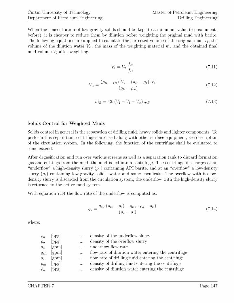
Curtin University of TechnologyDepartment of Petroleum Engineering
Master of Petroleum EngineeringDrilling Engineering
When the concentration of low-gravity solids should be kept to a minimum value (see commentsbefore), it is cheaper to reduce them by dilution before weighting the original mud with barite.The following equations are applied to calculate the corrected volume of the original mud V1, thevolume of the dilution water Vw, the mass of the weighting material m2 and the obtained finalmud volume V2 after weighting:
V1 = V2.fc2
fc1
(7.11)
Vw =(ρB − ρ2) .V2 − (ρB − ρ1) .V1
(ρB − ρw)(7.12)
mB = 42. (V2 − V1 − Vw) .ρB (7.13)
Solids Control for Weighted Muds
Solids control in general is the separation of drilling fluid, heavy solids and lighter components. Toperform this separation, centrifuges are used along with other surface equipment, see descriptionof the circulation system. In the following, the function of the centrifuge shall be evaluated tosome extend.
After degasification and run over various screens as well as a separation tank to discard formationgas and cuttings from the mud, the mud is fed into a centrifuge. The centrifuge discharges at an“underflow” a high-density slurry (ρu) containing API barite, and at an “overflow” a low-densityslurry (ρo) containing low-gravity solids, water and some chemicals. The overflow with its low-density slurry is discarded from the circulation system, the underflow with the high-density slurryis returned to the active mud system.
With equation 7.14 the flow rate of the underflow is computed as:
qu =qm. (ρm − ρo) − qw1. (ρo − ρw)
(ρu − ρo)(7.14)
where:
ρu [ppg] ... density of the underflow slurryρo [ppg] ... density of the overflow slurryqu [gpm] ... underflow flow rateqw1 [gpm] ... flow rate of dilution water entering the centrifugeqm [gpm] ... flow rate of drilling fluid entering the centrifugeρm [ppg] ... density of drilling fluid entering the centrifugeρw [ppg] ... density of dilution water entering the centrifuge
CHAPTER 7 Page 147
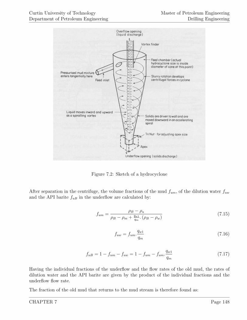
Curtin University of TechnologyDepartment of Petroleum Engineering
Master of Petroleum EngineeringDrilling Engineering
Figure 7.2: Sketch of a hydrocyclone
After separation in the centrifuge, the volume fractions of the mud fum, of the dilution water fuw
and the API barite fuB in the underflow are calculated by:
fum =ρB − ρu
ρB − ρm + qw1
qm. (ρB − ρw)
(7.15)
fuw = fum.qw1
qm
(7.16)
fuB = 1 − fum − fuw = 1 − fum − fum.qw1
qm
(7.17)
Having the individual fractions of the underflow and the flow rates of the old mud, the rates ofdilution water and the API barite are given by the product of the individual fractions and theunderflow flow rate.
The fraction of the old mud that returns to the mud stream is therefore found as:
CHAPTER 7 Page 148
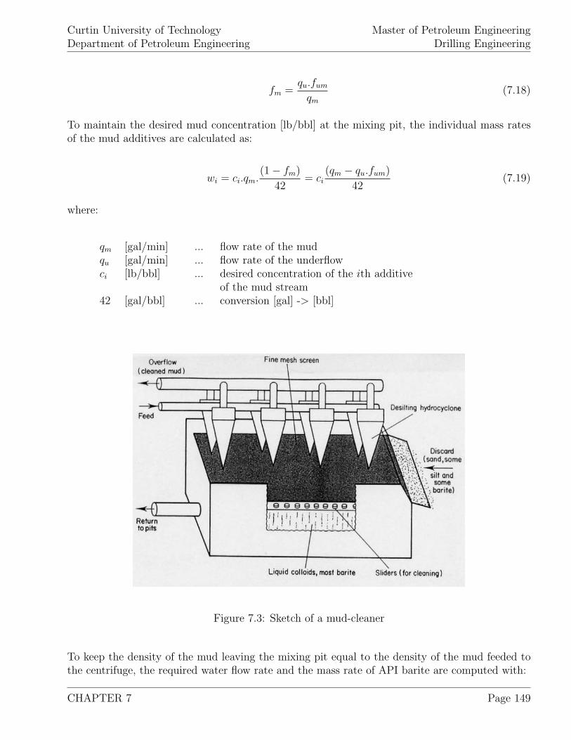
Curtin University of TechnologyDepartment of Petroleum Engineering
Master of Petroleum EngineeringDrilling Engineering
fm =qu.fum
qm
(7.18)
To maintain the desired mud concentration [lb/bbl] at the mixing pit, the individual mass ratesof the mud additives are calculated as:
wi = ci.qm.(1 − fm)
42= ci
(qm − qu.fum)
42(7.19)
where:
qm [gal/min] ... flow rate of the mudqu [gal/min] ... flow rate of the underflowci [lb/bbl] ... desired concentration of the ith additive
of the mud stream42 [gal/bbl] ... conversion [gal] -> [bbl]
Figure 7.3: Sketch of a mud-cleaner
To keep the density of the mud leaving the mixing pit equal to the density of the mud feeded tothe centrifuge, the required water flow rate and the mass rate of API barite are computed with:
CHAPTER 7 Page 149
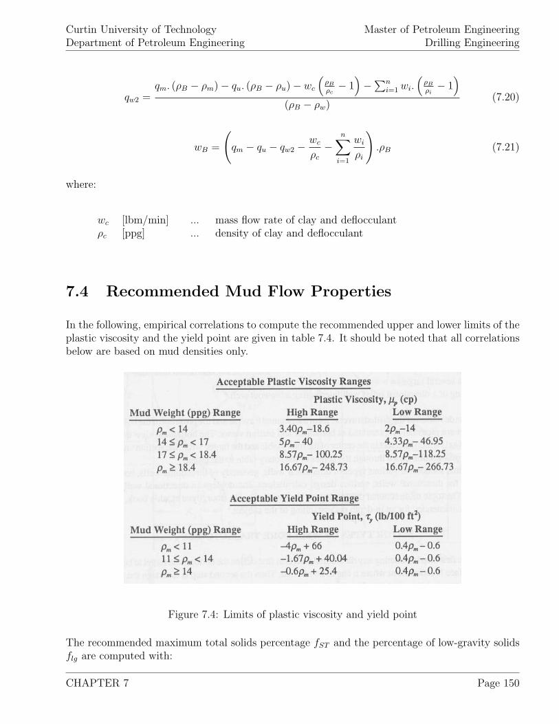
Curtin University of TechnologyDepartment of Petroleum Engineering
Master of Petroleum EngineeringDrilling Engineering
qw2 =qm. (ρB − ρm) − qu. (ρB − ρu) − wc
(ρB
ρc− 1)−∑n
i=1 wi.(
ρB
ρi− 1)
(ρB − ρw)(7.20)
wB =
(qm − qu − qw2 − wc
ρc
−n∑
i=1
wi
ρi
).ρB (7.21)
where:
wc [lbm/min] ... mass flow rate of clay and deflocculantρc [ppg] ... density of clay and deflocculant
7.4 Recommended Mud Flow Properties
In the following, empirical correlations to compute the recommended upper and lower limits of theplastic viscosity and the yield point are given in table 7.4. It should be noted that all correlationsbelow are based on mud densities only.
Figure 7.4: Limits of plastic viscosity and yield point
The recommended maximum total solids percentage fST and the percentage of low-gravity solidsflg are computed with:
CHAPTER 7 Page 150

Curtin University of TechnologyDepartment of Petroleum Engineering
Master of Petroleum EngineeringDrilling Engineering
fST = 2.917.ρm − 14.17 (7.22)
flg =100. (8.33 − ρm + 26.67.fST )
13.3(7.23)
where:
ρm [ppg] ... mud density
CHAPTER 7 Page 151
Curtin University of TechnologyDepartment of Petroleum Engineering
Master of Petroleum EngineeringDrilling Engineering
7.5 Examples
1. The pH-value of a drilling fluid is to be raised from 8 to 11.5. What is the amount of caustic,having a molecular weight of 40 required?
2. When 150 [lbm] of API barite, 40 [lbm] of bentonite and 1 [bbl] of water are mixed, what isthe resulting density?
3. When 70 [lbm] of calcium chloride is mixed with 1 [bbl] of water, what is the resulting density?
4. 700 [bbl] of mud have to be increased in density from 13 [ppg] to 15 [ppg] by adding of APIbarite. Since the mud thickness has to be maintained, 1 [gal] of water is added with every 100 [lb]of barite. Calculate the total amount of water and barite required when there is no limitation inthe final volume.
5. When 1,000 [bbl] of mud have to be increased from 10 [ppg] to 13 [ppg] mud weight by addingAPI barite, the total volume is limited to 1,000 [bbl]. How much old mud has to be discarded andwhat is the weight of the added API barite?
6. Using the data from example 5., the volume fraction of low-gravity solids must be reducedfrom 0.06 to 0.035 by adding water. Compute the API barite and water to be added as well asthe amount of old mud to be discarded.
7. A centrifuge is fed by a 15 [ppg] mud and 8.33 [ppg] dilution water at rates of 30 [gpm] and 15[gpm] respectively. The overflow has a density of 11 [ppg], the underflow 25 [ppg]. Assuming thatthe mud contains 30 [lb/bbl] bentonite and 15 [lb/bbl] deflocculant, determine the rates to addbentonite, deflocculant, water and API barite to maintain the mud properties at the mixing pit.
CHAPTER 7 Page 152
Curtin University of TechnologyDepartment of Petroleum Engineering
Master of Petroleum EngineeringDrilling Engineering
Chapter 8
Casing Design
Casing costs compromise one of the largest cost items of the drilling project. Therefore propperplanning of casing setting depths and casing selection is vital to realise a cost effective and safewell. The casings themselves fulfill multiple functions that can be summarized as:
1. Isolate porous formations with different fluid-pressure regimes from contaminating the payzone,
2. Prevent near surface fresh water zones from contamination with drilling mud,
3. Protect the hole from caving in,
4. Provide a connection and support of the wellhead equipment,
5. Provide exact dimensions for running testing, completion and production subsurface equip-ment.
8.1 Casing Types
According to the different functions, the total casing program consists of different casings strings.
8.1.1 Conductor Casing
The function of the conductor is to enable circulation of the drilling fluid to the shale shakerswithout eroding the surface sediments directly below the rig foundation. The conductor preventsthe subsequent casings from corrosion and may partly support the wellhead weight.
Commonly a diverter is installed on top of the conductor casing to divert an unexpected inflow offormation fluids into the wellbore away from the rig-site and the personal.
Conductor setting depths are in the range of 150 to 600 [ft], their seizes range from 36 to 20 [in].
CHAPTER 8 Page 153
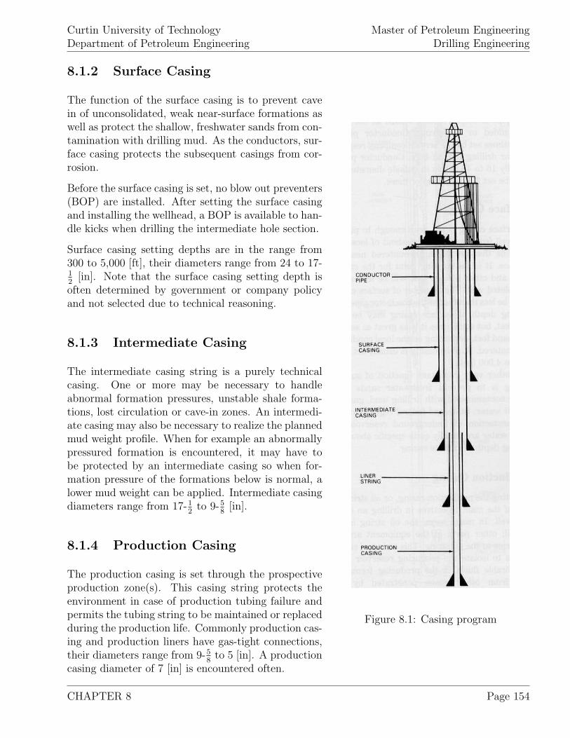
Curtin University of TechnologyDepartment of Petroleum Engineering
Master of Petroleum EngineeringDrilling Engineering
8.1.2 Surface Casing
Figure 8.1: Casing program
The function of the surface casing is to prevent cavein of unconsolidated, weak near-surface formations aswell as protect the shallow, freshwater sands from con-tamination with drilling mud. As the conductors, sur-face casing protects the subsequent casings from cor-rosion.
Before the surface casing is set, no blow out preventers(BOP) are installed. After setting the surface casingand installing the wellhead, a BOP is available to han-dle kicks when drilling the intermediate hole section.
Surface casing setting depths are in the range from300 to 5,000 [ft], their diameters range from 24 to 17-12
[in]. Note that the surface casing setting depth isoften determined by government or company policyand not selected due to technical reasoning.
8.1.3 Intermediate Casing
The intermediate casing string is a purely technicalcasing. One or more may be necessary to handleabnormal formation pressures, unstable shale forma-tions, lost circulation or cave-in zones. An intermedi-ate casing may also be necessary to realize the plannedmud weight profile. When for example an abnormallypressured formation is encountered, it may have tobe protected by an intermediate casing so when for-mation pressure of the formations below is normal, alower mud weight can be applied. Intermediate casingdiameters range from 17-1
2to 9-5
8[in].
8.1.4 Production Casing
The production casing is set through the prospectiveproduction zone(s). This casing string protects theenvironment in case of production tubing failure andpermits the tubing string to be maintained or replacedduring the production life. Commonly production cas-ing and production liners have gas-tight connections,their diameters range from 9-5
8to 5 [in]. A production
casing diameter of 7 [in] is encountered often.
CHAPTER 8 Page 154
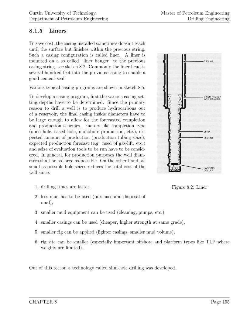
Curtin University of TechnologyDepartment of Petroleum Engineering
Master of Petroleum EngineeringDrilling Engineering
8.1.5 Liners
Figure 8.2: Liner
To save cost, the casing installed sometimes doesn’t reachuntil the surface but finishes within the previous string.Such a casing configuration is called liner. A liner ismounted on a so called “liner hanger” to the previouscasing string, see sketch 8.2. Commonly the liner head isseveral hundred feet into the previous casing to enable agood cement seal.
Various typical casing programs are shown in sketch 8.5.
To develop a casing program, first the various casing set-ting depths have to be determined. Since the primaryreason to drill a well is to produce hydrocarbons outof a reservoir, the final casing inside diameters have tobe large enough to allow for the forecasted completionand production schemes. Factors like completion type(open hole, cased hole, monobore production, etc.), ex-pected amount of production (production tubing seize),expected production forecast (e.g. need of gas-lift, etc.)and seize of evaluation tools to be run have to be consid-ered. In general, for production purposes the well diam-eters shall be as large as possible. On the other hand, assmall as possible hole seizes reduces the total cost of thewell since:
1. drilling times are faster,
2. less mud has to be used (purchase and disposal ofmud),
3. smaller mud equipment can be used (cleaning, pumps, etc.),
4. smaller casings can be used (cheaper, higher strength at same grade),
5. smaller rig can be applied (lighter casings, smaller mud volume),
6. rig site can be smaller (especially important offshore and platform types like TLP whereweights are limited).
Out of this reason a technology called slim-hole drilling was developed.
CHAPTER 8 Page 155
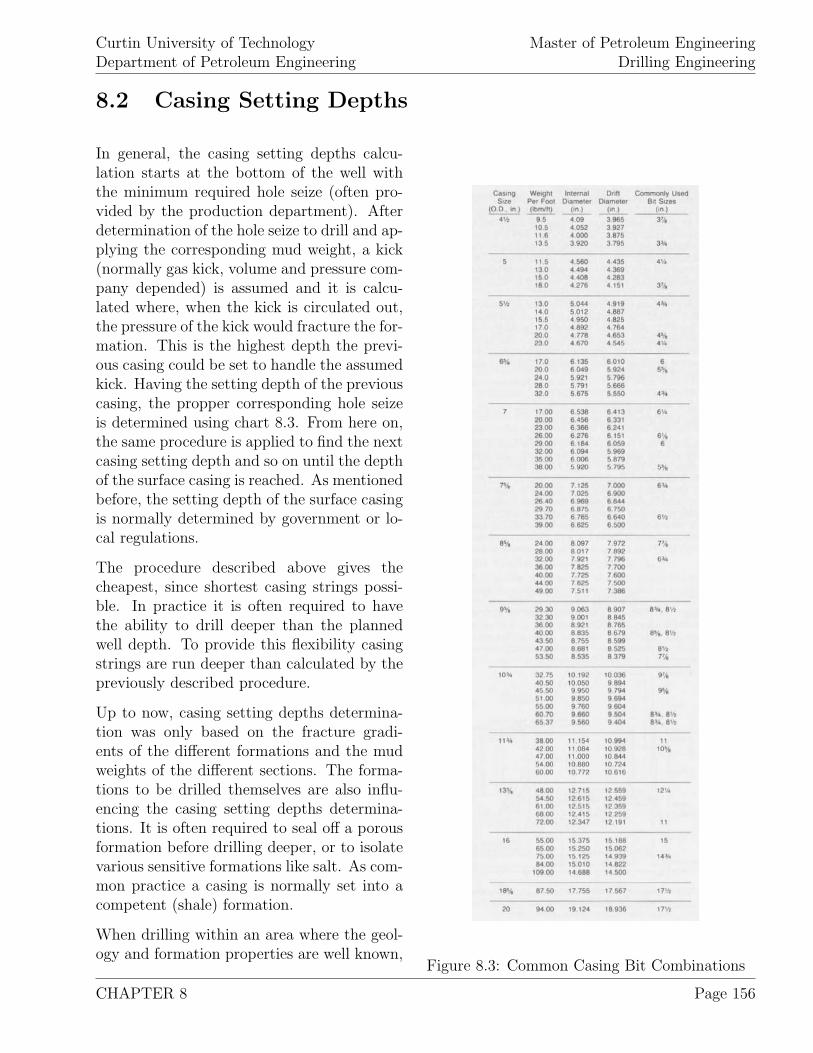
Curtin University of TechnologyDepartment of Petroleum Engineering
Master of Petroleum EngineeringDrilling Engineering
8.2 Casing Setting Depths
Figure 8.3: Common Casing Bit Combinations
In general, the casing setting depths calcu-lation starts at the bottom of the well withthe minimum required hole seize (often pro-vided by the production department). Afterdetermination of the hole seize to drill and ap-plying the corresponding mud weight, a kick(normally gas kick, volume and pressure com-pany depended) is assumed and it is calcu-lated where, when the kick is circulated out,the pressure of the kick would fracture the for-mation. This is the highest depth the previ-ous casing could be set to handle the assumedkick. Having the setting depth of the previouscasing, the propper corresponding hole seizeis determined using chart 8.3. From here on,the same procedure is applied to find the nextcasing setting depth and so on until the depthof the surface casing is reached. As mentionedbefore, the setting depth of the surface casingis normally determined by government or lo-cal regulations.
The procedure described above gives thecheapest, since shortest casing strings possi-ble. In practice it is often required to havethe ability to drill deeper than the plannedwell depth. To provide this flexibility casingstrings are run deeper than calculated by thepreviously described procedure.
Up to now, casing setting depths determina-tion was only based on the fracture gradi-ents of the different formations and the mudweights of the different sections. The forma-tions to be drilled themselves are also influ-encing the casing setting depths determina-tions. It is often required to seal off a porousformation before drilling deeper, or to isolatevarious sensitive formations like salt. As com-mon practice a casing is normally set into acompetent (shale) formation.
When drilling within an area where the geol-ogy and formation properties are well known,
CHAPTER 8 Page 156
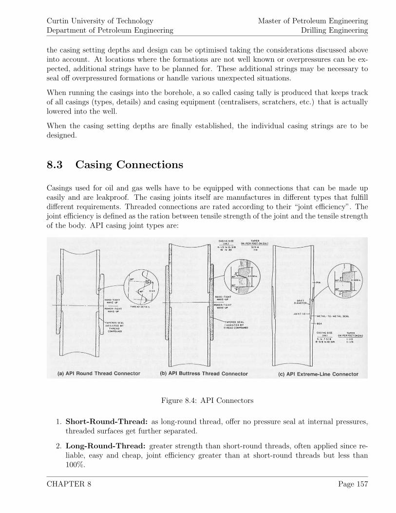
Curtin University of TechnologyDepartment of Petroleum Engineering
Master of Petroleum EngineeringDrilling Engineering
the casing setting depths and design can be optimised taking the considerations discussed aboveinto account. At locations where the formations are not well known or overpressures can be ex-pected, additional strings have to be planned for. These additional strings may be necessary toseal off overpressured formations or handle various unexpected situations.
When running the casings into the borehole, a so called casing tally is produced that keeps trackof all casings (types, details) and casing equipment (centralisers, scratchers, etc.) that is actuallylowered into the well.
When the casing setting depths are finally established, the individual casing strings are to bedesigned.
8.3 Casing Connections
Casings used for oil and gas wells have to be equipped with connections that can be made upeasily and are leakproof. The casing joints itself are manufactures in different types that fulfilldifferent requirements. Threaded connections are rated according to their “joint efficiency”. Thejoint efficiency is defined as the ration between tensile strength of the joint and the tensile strengthof the body. API casing joint types are:
Figure 8.4: API Connectors
1. Short-Round-Thread: as long-round thread, offer no pressure seal at internal pressures,threaded surfaces get further separated.
2. Long-Round-Thread: greater strength than short-round threads, often applied since re-liable, easy and cheap, joint efficiency greater than at short-round threads but less than100%.
CHAPTER 8 Page 157
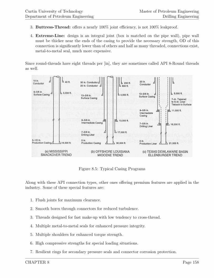
Curtin University of TechnologyDepartment of Petroleum Engineering
Master of Petroleum EngineeringDrilling Engineering
3. Buttress-Thread: offers a nearly 100% joint efficiency, is not 100% leakproof.
4. Extreme-Line: design is an integral joint (box is matched on the pipe wall), pipe wallmust be thicker near the ends of the casing to provide the necessary strength, OD of thisconnection is significantly lower than of others and half as many threaded, connections exist,metal-to-metal seal, much more expensive.
Since round-threads have eight threads per [in], they are sometimes called API 8-Round threadsas well.
Figure 8.5: Typical Casing Programs
Along with these API connection types, other ones offering premium features are applied in theindustry. Some of these special features are:
1. Flush joints for maximum clearance.
2. Smooth bores through connectors for reduced turbulence.
3. Threads designed for fast make-up with low tendency to cross-thread.
4. Multiple metal-to-metal seals for enhanced pressure integrity.
5. Multiple shoulders for enhanced torque strength.
6. High compressive strengths for special loading situations.
7. Resilient rings for secondary pressure seals and connector corrosion protection.
CHAPTER 8 Page 158
Curtin University of TechnologyDepartment of Petroleum Engineering
Master of Petroleum EngineeringDrilling Engineering
As drillpipes, casings are manufactured in different length ranges:
Range 1 16 to 25 [ft],Range 2 25 to 34 [ft],Range 3 34 to 48 [ft],
8.4 API Casing Performance Properties
The American Petroleum Institute (API) has developed internationally accepted standards foroilfield tubulars and summarised them in bulletins that contain the minimum performance prop-erties and equations to compute these properties. It should be understood that these propertiesare guidelines (minimum requirements), for casing design calculations, the exact strength valuesprovided by the individual manufacture shall be applied.
A casing is defined by:
1. Casing outside diameter (OD),
2. Weight per unit length (this determines the wall thickness),
3. Grade of steel,
4. Type of coupling,
5. Length of joint.
To determine the strength of various casing materials, API has designated defined grades. Thegrading code consists of a letter followed by a number where the number gives the minimum yieldstrength of the material in thousands of [psi], the number is an arbitrary one (e.g. N-80). For wellsthat require very high tensile strength, collapse resistance or better corrosion resistance, non-APIcasings are used by the industry as well.
Tables 8.6 through 8.21 list API and some non-API ones as well as gives the minimum performanceproperties of them. To calculate the individual properties following equations can be applied:
Yield strength collapse pressure:
py = 2.σy
[do
t− 1
(do
t)2
](8.1)
Above equation is valid up to where do
tintersects (do
t)yp and thus the plastic deformation starts.
(do
t)yp is calculated as:
CHAPTER 8 Page 159
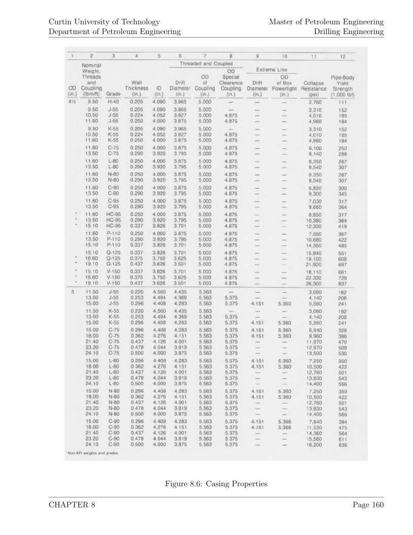
Curtin University of TechnologyDepartment of Petroleum Engineering
Master of Petroleum EngineeringDrilling Engineering
Figure 8.6: Casing Properties
CHAPTER 8 Page 160
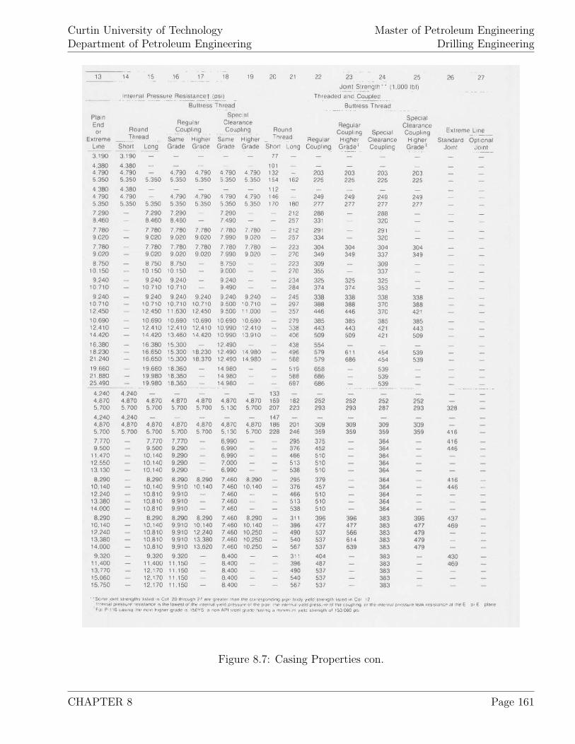
Curtin University of TechnologyDepartment of Petroleum Engineering
Master of Petroleum EngineeringDrilling Engineering
Figure 8.7: Casing Properties con.
CHAPTER 8 Page 161
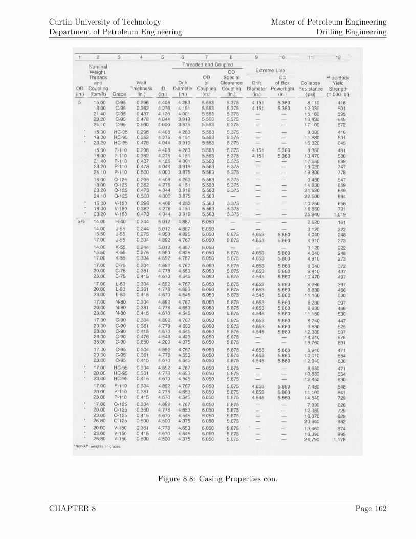
Curtin University of TechnologyDepartment of Petroleum Engineering
Master of Petroleum EngineeringDrilling Engineering
Figure 8.8: Casing Properties con.
CHAPTER 8 Page 162
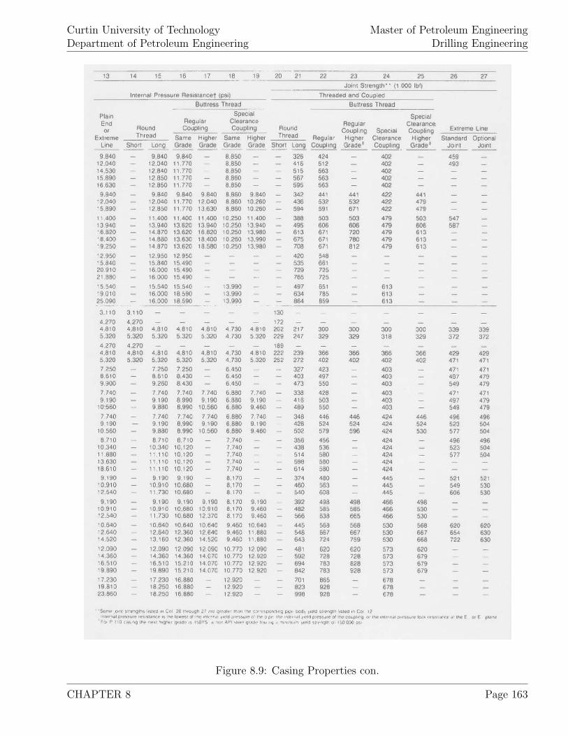
Curtin University of TechnologyDepartment of Petroleum Engineering
Master of Petroleum EngineeringDrilling Engineering
Figure 8.9: Casing Properties con.
CHAPTER 8 Page 163
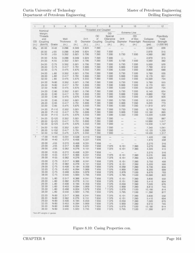
Curtin University of TechnologyDepartment of Petroleum Engineering
Master of Petroleum EngineeringDrilling Engineering
Figure 8.10: Casing Properties con.
CHAPTER 8 Page 164
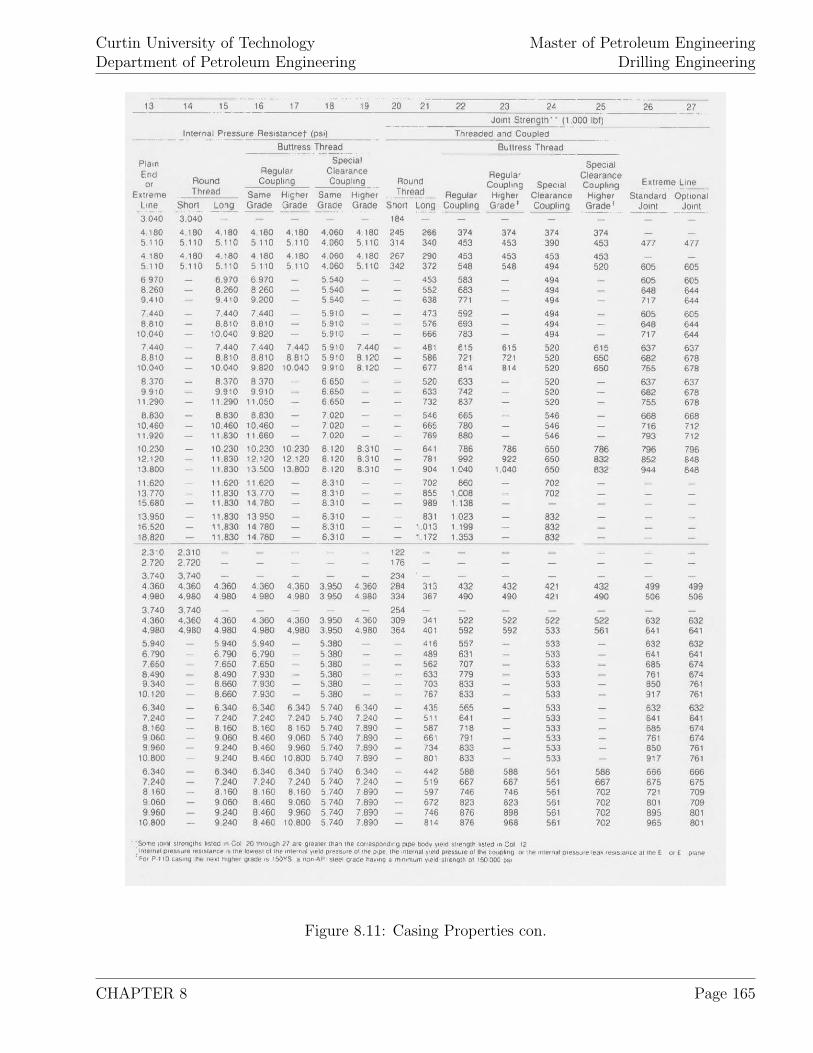
Curtin University of TechnologyDepartment of Petroleum Engineering
Master of Petroleum EngineeringDrilling Engineering
Figure 8.11: Casing Properties con.
CHAPTER 8 Page 165
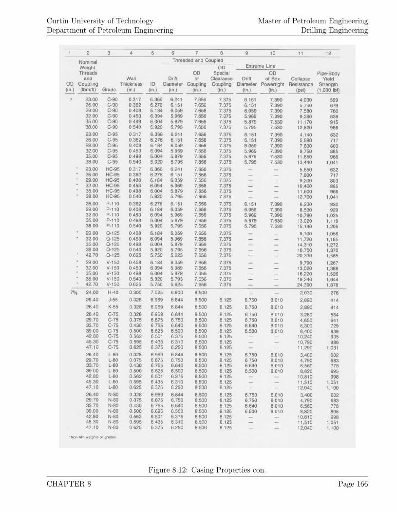
Curtin University of TechnologyDepartment of Petroleum Engineering
Master of Petroleum EngineeringDrilling Engineering
Figure 8.12: Casing Properties con.
CHAPTER 8 Page 166
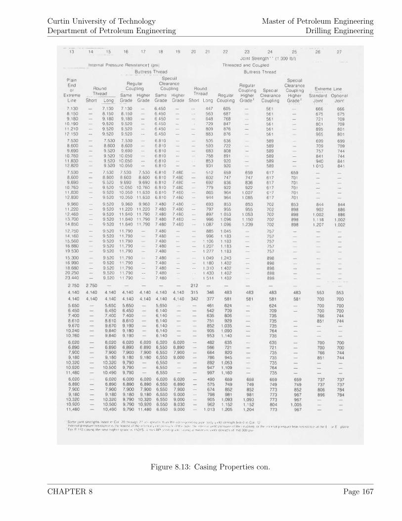
Curtin University of TechnologyDepartment of Petroleum Engineering
Master of Petroleum EngineeringDrilling Engineering
Figure 8.13: Casing Properties con.
CHAPTER 8 Page 167
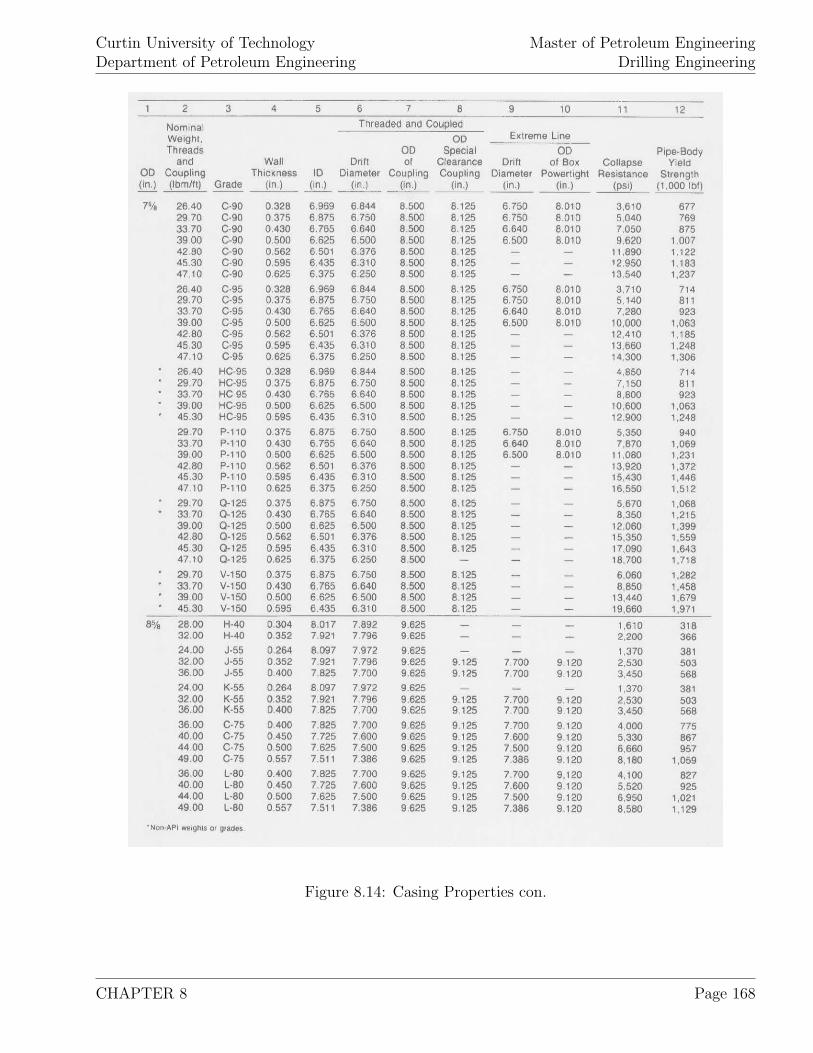
Curtin University of TechnologyDepartment of Petroleum Engineering
Master of Petroleum EngineeringDrilling Engineering
Figure 8.14: Casing Properties con.
CHAPTER 8 Page 168
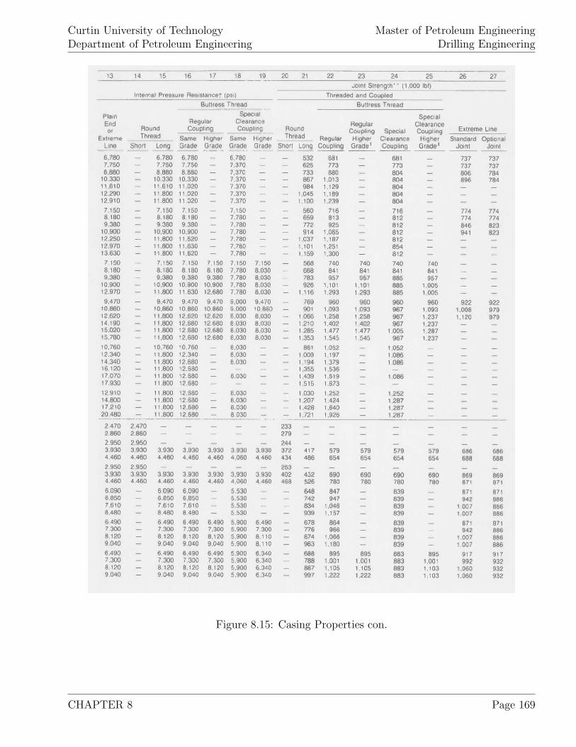
Curtin University of TechnologyDepartment of Petroleum Engineering
Master of Petroleum EngineeringDrilling Engineering
Figure 8.15: Casing Properties con.
CHAPTER 8 Page 169
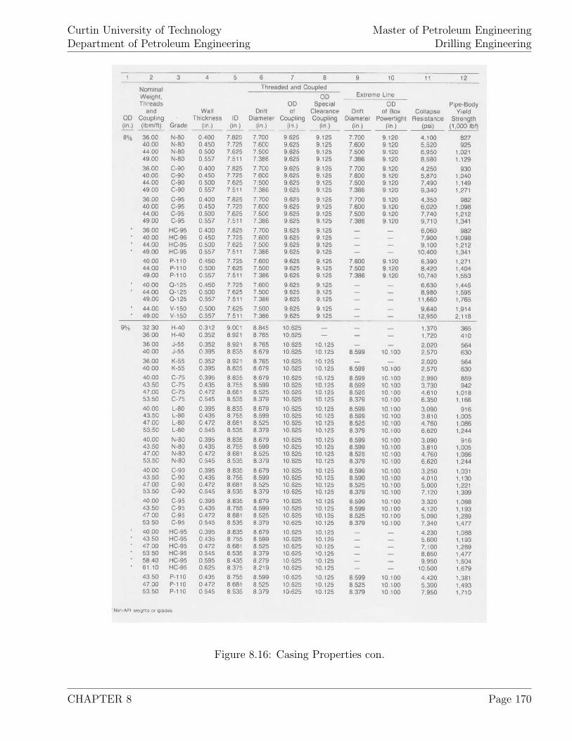
Curtin University of TechnologyDepartment of Petroleum Engineering
Master of Petroleum EngineeringDrilling Engineering
Figure 8.16: Casing Properties con.
CHAPTER 8 Page 170
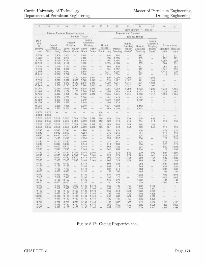
Curtin University of TechnologyDepartment of Petroleum Engineering
Master of Petroleum EngineeringDrilling Engineering
Figure 8.17: Casing Properties con.
CHAPTER 8 Page 171
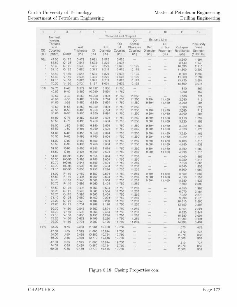
Curtin University of TechnologyDepartment of Petroleum Engineering
Master of Petroleum EngineeringDrilling Engineering
Figure 8.18: Casing Properties con.
CHAPTER 8 Page 172
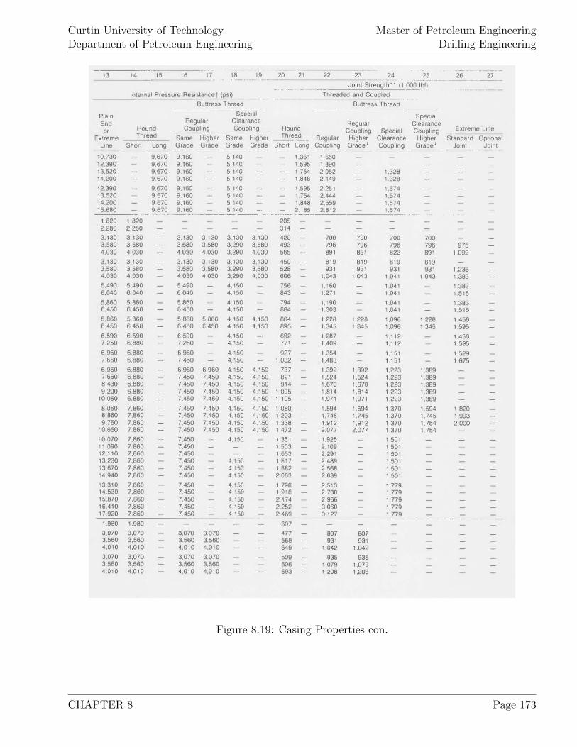
Curtin University of TechnologyDepartment of Petroleum Engineering
Master of Petroleum EngineeringDrilling Engineering
Figure 8.19: Casing Properties con.
CHAPTER 8 Page 173
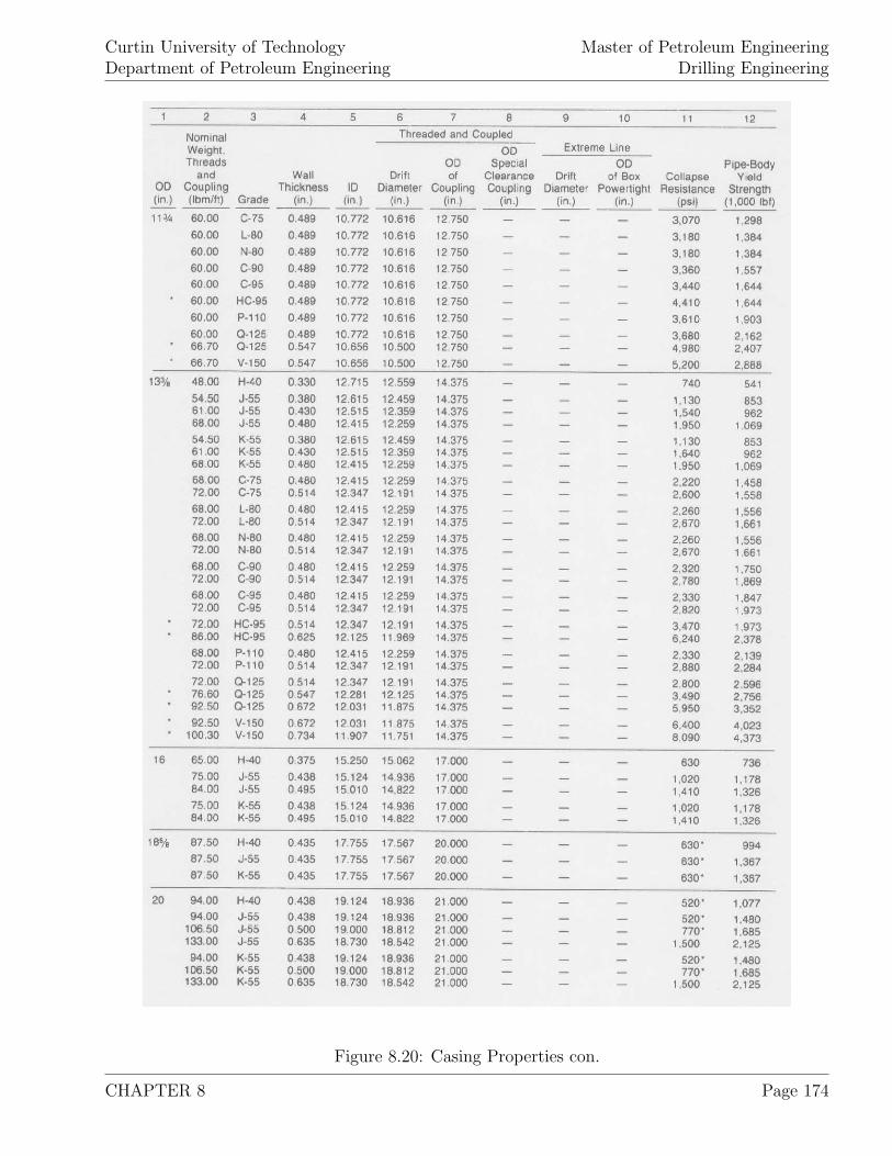
Curtin University of TechnologyDepartment of Petroleum Engineering
Master of Petroleum EngineeringDrilling Engineering
Figure 8.20: Casing Properties con.
CHAPTER 8 Page 174
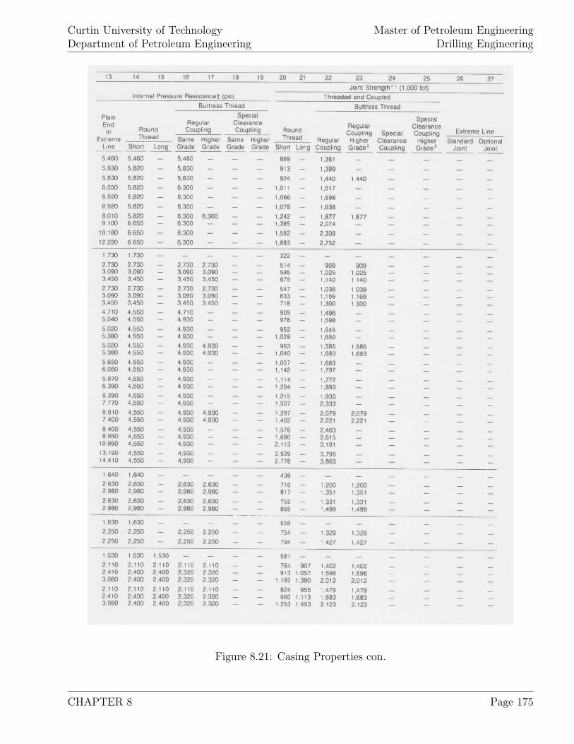
Curtin University of TechnologyDepartment of Petroleum Engineering
Master of Petroleum EngineeringDrilling Engineering
Figure 8.21: Casing Properties con.
CHAPTER 8 Page 175
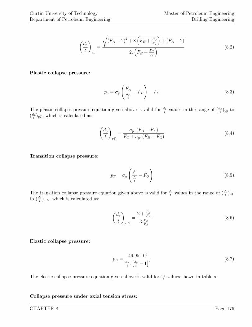
Curtin University of TechnologyDepartment of Petroleum Engineering
Master of Petroleum EngineeringDrilling Engineering
(do
t
)yp
=
√(FA − 2)2 + 8
(FB + FC
σy
)+ (FA − 2)
2.(FB + FC
σy
) (8.2)
Plastic collapse pressure:
pp = σy
(FA
do
t
− FB
)− FC (8.3)
The plastic collapse pressure equation given above is valid for do
tvalues in the range of (do
t)yp to
(do
t)pT , which is calculated as:
(do
t
)pT
=σy. (FA − FF )
FC + σy. (FB − FG)(8.4)
Transition collapse pressure:
pT = σy
(Fdo
t
− FG
)(8.5)
The transition collapse pressure equation given above is valid for do
tvalues in the range of (do
t)pT
to (do
t)TE, which is calculated as:
(do
t
)TE
=2 + FB
FA
3.FB
FA
(8.6)
Elastic collapse pressure:
pE =49.95.106
do
t.[
do
t− 1]2 (8.7)
The elastic collapse pressure equation given above is valid for do
tvalues shown in table x.
Collapse pressure under axial tension stress:
CHAPTER 8 Page 176
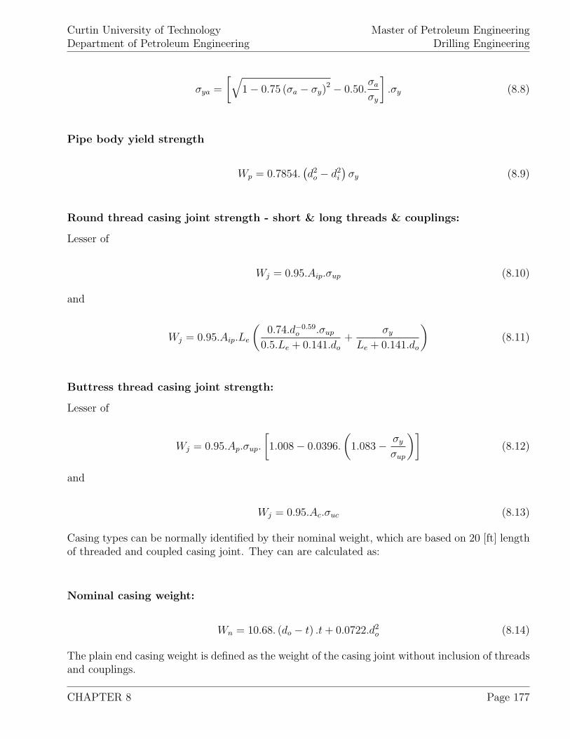
Curtin University of TechnologyDepartment of Petroleum Engineering
Master of Petroleum EngineeringDrilling Engineering
σya =
[√1 − 0.75 (σa − σy)
2 − 0.50.σa
σy
].σy (8.8)
Pipe body yield strength
Wp = 0.7854.(d2
o − d2i
)σy (8.9)
Round thread casing joint strength - short & long threads & couplings:
Lesser of
Wj = 0.95.Aip.σup (8.10)
and
Wj = 0.95.Aip.Le
(0.74.d−0.59
o .σup
0.5.Le + 0.141.do
+σy
Le + 0.141.do
)(8.11)
Buttress thread casing joint strength:
Lesser of
Wj = 0.95.Ap.σup.
[1.008 − 0.0396.
(1.083 − σy
σup
)](8.12)
and
Wj = 0.95.Ac.σuc (8.13)
Casing types can be normally identified by their nominal weight, which are based on 20 [ft] lengthof threaded and coupled casing joint. They can are calculated as:
Nominal casing weight:
Wn = 10.68. (do − t) .t + 0.0722.d2o (8.14)
The plain end casing weight is defined as the weight of the casing joint without inclusion of threadsand couplings.
CHAPTER 8 Page 177
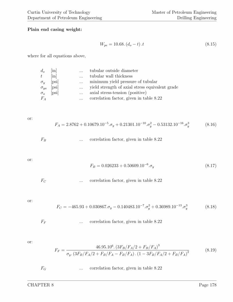
Curtin University of TechnologyDepartment of Petroleum Engineering
Master of Petroleum EngineeringDrilling Engineering
Plain end casing weight:
Wpe = 10.68. (do − t) .t (8.15)
where for all equations above,
do [in] ... tubular outside diametert [in] ... tubular wall thicknessσy [psi] ... minimum yield pressure of tubularσya [psi] ... yield strength of axial stress equivalent gradeσa [psi] ... axial stress-tension (positive)FA ... correlation factor, given in table 8.22
or:
FA = 2.8762 + 0.10679.10−5.σy + 0.21301.10−10.σ2y − 0.53132.10−16.σ3
y (8.16)
FB ... correlation factor, given in table 8.22
or:
FB = 0.026233 + 0.50609.10−6.σy (8.17)
FC ... correlation factor, given in table 8.22
or:
FC = −465.93 + 0.030867.σy − 0.140483.10−7.σ2y + 0.36989.10−13.σ3
y (8.18)
FF ... correlation factor, given in table 8.22
or:
FF =46.95.106. (3FB/FA/2 + FB/FA)3
σy. (3FB/FA/2 + FB/FA − FB/FA) . (1 − 3FB/FA/2 + FB/FA)2 (8.19)
FG ... correlation factor, given in table 8.22
CHAPTER 8 Page 178
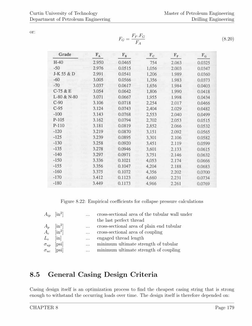
Curtin University of TechnologyDepartment of Petroleum Engineering
Master of Petroleum EngineeringDrilling Engineering
or:
FG =FF .FG
FA
(8.20)
Figure 8.22: Empirical coefficients for collapse pressure calculations
Aip [in2] ... cross-sectional area of the tubular wall underthe last perfect thread
Ap [in2] ... cross-sectional area of plain end tubularAc [in2] ... cross-sectional area of couplingLe [in] ... engaged thread lengthσup [psi] ... minimum ultimate strength of tubularσuc [psi] ... minimum ultimate strength of coupling
8.5 General Casing Design Criteria
Casing design itself is an optimization process to find the cheapest casing string that is strongenough to withstand the occurring loads over time. The design itself is therefore depended on:
CHAPTER 8 Page 179
Curtin University of TechnologyDepartment of Petroleum Engineering
Master of Petroleum EngineeringDrilling Engineering
1. Loading conditions during life of well (drilling phase, completion procedures, workover op-erations, and operation phase),
2. strength of the formation at the casing shoe (assumed fracture pressure during planning andverified by the formation integrity test),
3. availability and real price of individual casing strings,
4. expected deterioration of the casing due to production and expected completion fluid set-tlement.
It should be noted that the loading conditions are subjective and based on company policies,governmental regulations and best practices. Regarding real casing prices, casing types currentlyon stock and general availability (purchase of manufacturing lot) can have a major selectionimplication.
Similar to the drillstring, casings are normally designed for burst, collapse, tension, shock loadsand biaxial stresses. Different safety margins or safety factors are demanded by company policiesor government regulations and have to be satisfied.
To calculate the burst and collapse pressure the casing has to be designed for, the differentialpressure (outside pressure - inside pressure) is determined for the worst case to appear.
For burst pressure, the maximum formation pressure anticipated while drilling the next section isassumed. Thus the highest burst pressure is expected to be at the top of the casing and least atthe casing shoe (hydrostatic pressure at annulus to counterbalance). When the production tubingis assumed to leak gas to the casing, this burst pressure profile is reversed.
For collapse pressure, it is assumed that the mud inside the casing is lost to a weak or fracturedformation below. Thus the collapse pressure is due to the hydrostatic pressure of the fluid outsidethe casing and therefore maximum at the casing shoe and zero at the casing top. In this way thecollapse pressure can be calculated with:
pc = 0.052.ρout.D (8.21)
The tensile forces acting on the casing are due to its weight, bending forces and shock loading atlanding. It should be noted that at highly deviated wells, landing the casing is only possible whenrun partly or totally empty. This is also called “floating the casing in”. Here the casing, whenrun, is closed at the shoe and its inside is not filled with mud. This causes a buoyancy to suchan extend that the casing may has to be forced into the well. The casing dimensions where thebuoyancy counterbalances the casing weight is given by:
ρst.g.h.(d2
o − d2i
).π
4= ρm.g.h.d2
o.π
4(8.22)
d2o − d2
i
d2o
=ρm
ρst
(8.23)
CHAPTER 8 Page 180
Curtin University of TechnologyDepartment of Petroleum Engineering
Master of Petroleum EngineeringDrilling Engineering
For tensile loading, the topmost joint is considered as the weakest one since it carries all the casingweight.
When casings have to carry inner strings as well (conductor, surface and intermediate casing),they are subjective to compression loads. Thus production casings and casings where liners arebelow are free from these loads.
Since the casing is in general subjected to a combination of external pressures and its own weight,they are under a biaxial stress regime. This will reduce the collapse resistance of the casing.The amount of collapse resistance reduction can be calculated with the methods described fordrillstring calculation.
In addition to the general casing loads discussed above, casings are also subjected to bending withtongs, slip crushing, wear due to rotation of the drillstring and running tools into the hole as wellas corrosion and fatigue.
As mentioned above, the actual loadings of the casings have to be lower than the individual casingstrengths. This is often expressed with safety factors. Applying propper safety factors accountfor the uncertainty in estimation the real loadings as well as the change of casing properties overthe lifetime of the well. Commonly chosen safety factors are:
Collapse strength: 0.85 - 1.125Joint strength: 1.60 - 1.80Plain-end yield strength: 1.25Internal yield pressure: 1.0
In practice, sophisticated casing design computer programs are available in companies that allowcomplex casing loading scenarios and the design of casing strings with various casing pipes (differ-ent grades) as well as variable diameters for one casing string. Such casings are generally referredto as “combination string”.
8.6 Graphical Method for Casing Design
The graphical method to select casings with the suitable grades, weights and section lengths is themost often applied one. Here, the individual loads (burst, collapse and tensions) are representedas graphs on a pressure vs. depth diagram. The minimum strength values of the individual casingsections are drawn as vertical lines where the suitable ones have to be to the right of the respectiveloads (stronger). In this way, the depth where the minimum safety (load and casing minimumstrength are closest) can be easily spotted and the respective factors calculated.
To construct the diagram, following procedures can be applied:
CHAPTER 8 Page 181
Curtin University of TechnologyDepartment of Petroleum Engineering
Master of Petroleum EngineeringDrilling Engineering
Burst line:
1. Calculate the external pressure due to an assumed fluid column of 0.465 [psi/ft] (salt-saturated completion fluid),
2. Calculate the internal pressure due to the maximum anticipated pressures when drilling thenext section,
3. Calculate the burst pressure pb as the difference between the external and the internalpressures,
pb = pf − (TD − CSD) .Gf − 0.053.ρm.CSD (8.24)
where:
pf [ft] ... maximum anticipated formation pressure to drill next sectionTD [ft] ... total depth (TVD)CSD [ft] ... casing setting depth (TVD)Gf [psi/ft] ... formation fluid gradientρm [ppg ... mud density
In this way the burst pressure at the surface is calculated as:
pb = pf − TD.Gf (8.25)
4. On the pressure vs. depth graph draw a stright line between the maximum Burst pressureat the casing top and the minimum burst pressure at the casing shoe,
5. Select from tables 8.6 through 8.21 casings with burst resistance above the burst loadingline,
6. Draw the vertical lines of the casings with the individual grades,
7. The individual intersections of the burst loading line and the casing burst resistances deter-mine the depths from which upwards the casing grades can be used.
Collapse line:
1. Calculate the external and internal pressure due to the mud columns outside and inside thecasing,
2. Calculate the collapse pressure pc as the difference between the external and the internalpressures,
CHAPTER 8 Page 182
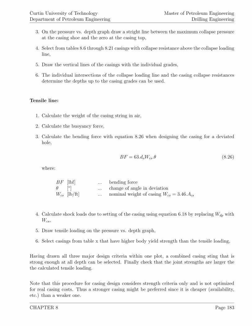
Curtin University of TechnologyDepartment of Petroleum Engineering
Master of Petroleum EngineeringDrilling Engineering
3. On the pressure vs. depth graph draw a stright line between the maximum collapse pressureat the casing shoe and the zero at the casing top,
4. Select from tables 8.6 through 8.21 casings with collapse resistance above the collapse loadingline,
5. Draw the vertical lines of the casings with the individual grades,
6. The individual intersections of the collapse loading line and the casing collapse resistancesdetermine the depths up to the casing grades can be used.
Tensile line:
1. Calculate the weight of the casing string in air,
2. Calculate the buoyancy force,
3. Calculate the bending force with equation 8.26 when designing the casing for a deviatedhole,
BF = 63.doWcs.θ (8.26)
where:
BF [lbf] ... bending forceθ [◦] ... change of angle in deviationWcs [lb/ft] ... nominal weight of casing Wcs = 3.46.Acs
4. Calculate shock loads due to setting of the casing using equation 6.18 by replacing Wdp withWcs,
5. Draw tensile loading on the pressure vs. depth graph,
6. Select casings from table x that have higher body yield strength than the tensile loading,
Having drawn all three major design criteria within one plot, a combined casing sting that isstrong enough at all depth can be selected. Finally check that the joint strengths are larger thethe calculated tensile loading.
Note that this procedure for casing design considers strength criteria only and is not optimizedfor real casing costs. Thus a stronger casing might be preferred since it is cheaper (availability,etc.) than a weaker one.
CHAPTER 8 Page 183
Curtin University of TechnologyDepartment of Petroleum Engineering
Master of Petroleum EngineeringDrilling Engineering
Figure 8.23: Sketch of graphical design of a casing string
8.7 Maximum Load Casing Design for Intermediate Cas-
ing
The load criteria assumed above are based on a 100 % empty casing (collapse) and a 100 % gas-kickfilled (burst) one respectively. These are very conservative assumptions that lead to over-designcausing unnecessary high cost of the casing string. If standard drilling procedures and precautionsare followed, these assumptions are not to be expected. When drilling into a weak or fracturedformation that causes lost circulation, the remaining fluid hight can be estimated with:
L =0.465.CSD
ρm.19.25(8.27)
where:
ρm [ppg] ... weight of mud used to drill next section.
For this reason the casing is supported in the inside by the hydrostatic pressure of the remainingmud column of length L.
CHAPTER 8 Page 184
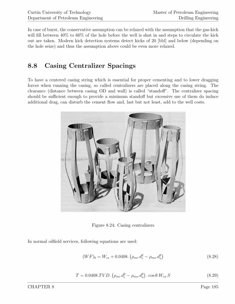
Curtin University of TechnologyDepartment of Petroleum Engineering
Master of Petroleum EngineeringDrilling Engineering
In case of burst, the conservative assumption can be relaxed with the assumption that the gas-kickwill fill between 40% to 60% of the hole before the well is shut in and steps to circulate the kickout are taken. Modern kick detection systems detect kicks of 20 [bbl] and below (depending onthe hole seize) and thus the assumption above could be even more relaxed.
8.8 Casing Centralizer Spacings
To have a centered casing string which is essential for proper cementing and to lower draggingforces when running the casing, so called centralizers are placed along the casing string. Theclearance (distance between casing OD and wall) is called “standoff”. The centralizer spacingshould be sufficient enough to provide a minimum standoff but excessive use of them do induceadditional drag, can disturb the cement flow and, last but not least, add to the well costs.
Figure 8.24: Casing centralizers
In normal oilfield services, following equations are used:
(WF )b = Wcs + 0.0408.(ρmi.d
2i − ρmo.d
2o
)(8.28)
T = 0.0408.TV D.(ρmi.d
2i − ρmo.d
2o
). cos θ.Wcs.S (8.29)
CHAPTER 8 Page 185
Curtin University of TechnologyDepartment of Petroleum Engineering
Master of Petroleum EngineeringDrilling Engineering
CS =F
0.0175.T.DLS + (WF )b . sin θ(8.30)
F = 2.T. sin
(DLS.
CS
2
)+ (WF )b .CS. sin θ (8.31)
where:
F [lbf] ... force on each centralizerCS [ft] ... spacing of centralizerWcs [lb/ft] ... nominal weight of casingθ [◦] ... average inclination angle near the centralizerT [lbf] ... tension in the casing at centralizerTV D [ft] ... true vertical depth to the casing shoeρmi [ppg] ... mud weight inside the casingρmo [ppg] ... mud weight outside the casingS [ft] ... distance of the centralizer from the casing shoe.DLS [◦/100 ft] ... dogleg severitydi [in] ... inside diameter of the casingdo [in] ... outside diameter of the casingS [ft] ... distance of casing shoe to particular centralizer
To control vertical travel of the centralizers, casing couplings or various types of attached stopsare applied.
8.9 Stretch in Casing
The elongation or stretch of tubular material resulting from pulling forces and its own weight ispart of the design calculation. As it can easily be understood, the amount of stretch depends onthe amount of pull, the length of the tubular, the elasticity of the material and its cross-sectionalarea. Following equations can be applied to calculate the tubular elongation:
Tubular freely suspended in fluid:
∆Lt = ∆L1 + ∆L2 + ∆L3 + F1.W2 + W3
W1
+ F2.W3
W2
+
C1. [Ls1.Ls2 + (Ls1 + Ls2) .Ls3] − C2
(L2
s2.W1
W2
+ L2s3.
W1 + W2
W3
)(8.32)
The tension stresses along the casing string after setting and cementing are given by:
CHAPTER 8 Page 186
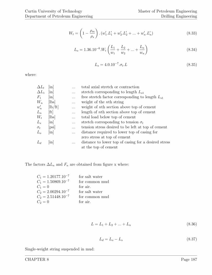
Curtin University of TechnologyDepartment of Petroleum Engineering
Master of Petroleum EngineeringDrilling Engineering
Wt =
(1 − ρm
ρs
). (w′
1.L′1 + w′
2.L′2 + ... + w′
n.L′n) (8.33)
Lo = 1.36.10−6.Wt
(L1
w1
+L2
w2
+ ... +Ln
wn
)(8.34)
Ls = 4.0.10−7.σt.L (8.35)
where:
∆Lt [in] ... total axial stretch or contraction∆L1 [in] ... stretch corresponding to length Ls1
F1 [in] ... free stretch factor corresponding to length Ls1
Wn [lbs] ... weight of the nth stringw′
n [lb/ft] ... weight of nth section above top of cementLn [ft] ... length of nth section above top of cementWt [lbs] ... total load below top of cementLs [in] ... stretch corresponding to tension σt
σt [psi] ... tension stress desired to be left at top of cementLo [in] ... distance required to lower top of casing for
zero stress at top of cementLd [in] ... distance to lower top of casing for a desired stress
at the top of cement
The factors ∆Ln and Fn are obtained from figure x where:
C1 = 1.20177.10−7 for salt waterC1 = 1.50869.10−7 for common mudC1 = 0 for air.C2 = 2.00294.10−7 for salt waterC2 = 2.51448.10−7 for common mudC2 = 0 for air.
L = L1 + L2 + ... + Ln (8.36)
Ld = Lo − Ls (8.37)
Single-weight string suspended in mud:
CHAPTER 8 Page 187

Curtin University of TechnologyDepartment of Petroleum Engineering
Master of Petroleum EngineeringDrilling Engineering
Lo = 1.1085.10−5. (D − L′) (8.38)
where:
D [ft] ... total depth of the well or length of the stringL′ [ft] ... length of casing below top of cement.
CHAPTER 8 Page 188
Curtin University of TechnologyDepartment of Petroleum Engineering
Master of Petroleum EngineeringDrilling Engineering
8.10 Examples
1. A 20 [in] conductor pipe is set in a 26 [in] hole at 400 [ft]. The mud weights for this well are8.69 [ppg] to drill the conductor and 8.96 [ppg] for the next section, a 17-1
2[in] hole reaching 6,250
[ft]. Design the conductor using 0.85 for collapse safety factor, 1.1 for burst safety factor and 1.8for the tension safety factor.
2. Continuing from example 1, design the 13-38
[in] intermediate casing which is run until 6,250[ft]. The next hole section is drilled with a 9.8 [ppg] mud to a depth of 10,000 [ft].
3. Continue from example 1 and 2, the 9-58
[in] casing, set at 10,000 [ft] is to be designed. Theretoa kick at 13,000 [ft] causes from a formation pressure of 0.57 [psi/ft] is assumed. The mud weightused to drill until 13,000 [ft] is 11.5 [ppg], the maximum dogleg severity at the hole is 3 [◦/ 100ft]. Following casings shall be assumed to be available for this well:
Grade: Weight [lb/ft] Collapse [psi] Burst [psi]C-75 43.5 3,750 5,930L-80 47.0 4,750 6,870C-95 53.5 7,330 9,410
4. Re-design the 9-58
[in] casing applying the released assumptions that a remaining mud is leftinside the hole and the kick fills the well bore to 50 % before shut in.
5. A well is to be drilled to 10,000 [ft] MD (4,200 [ft] TVD). At the gradual dogleg of the section6,020 [ft] with an inclination of 38◦ and a direction of N3◦ and 6,220 [ft], showing an inclinationof 46◦ and a direction of N7E◦, a centralizer is to be placed. To maintain a standoff of 1 [in]while bearing a wall force of 1,100 [lbf], the centralizer spacing is to be designed. ρmo = 12 [ppg],ρmi = 15 [ppg], Wcs = 53 [lb/ft], do = 9.625 [in], di = 8.535 [in]
CHAPTER 8 Page 189

Curtin University of TechnologyDepartment of Petroleum Engineering
Master of Petroleum EngineeringDrilling Engineering
CHAPTER 8 Page 190
Curtin University of TechnologyDepartment of Petroleum Engineering
Master of Petroleum EngineeringDrilling Engineering
Chapter 9
Directional Drilling and DeviationControl
A well is declared as a directional one when it follows a predescribed traverse or trajectory tointersect specific targets. Figure 9.1 through 9.8 illustrates different situations when directionalwell trajectories are planned for.
They can be necessary when:
1. Reaching a target which is below inaccessible or restricted areas such as a mountain, a highlypopulated area, a national park, etc.,
2. Multiple wells have to be drilled from one offshore platform to deplete large portions of areservoir from one structure,
3. Side tracking has to be done around a fish,
4. Fault drilling is necessary,
5. Salt dome drilling takes place,
6. Drilling a relief well to intersect a blowout well,
7. Sidetracking from an old well to explore different horizons and/or directions.
CHAPTER 9 Page 191
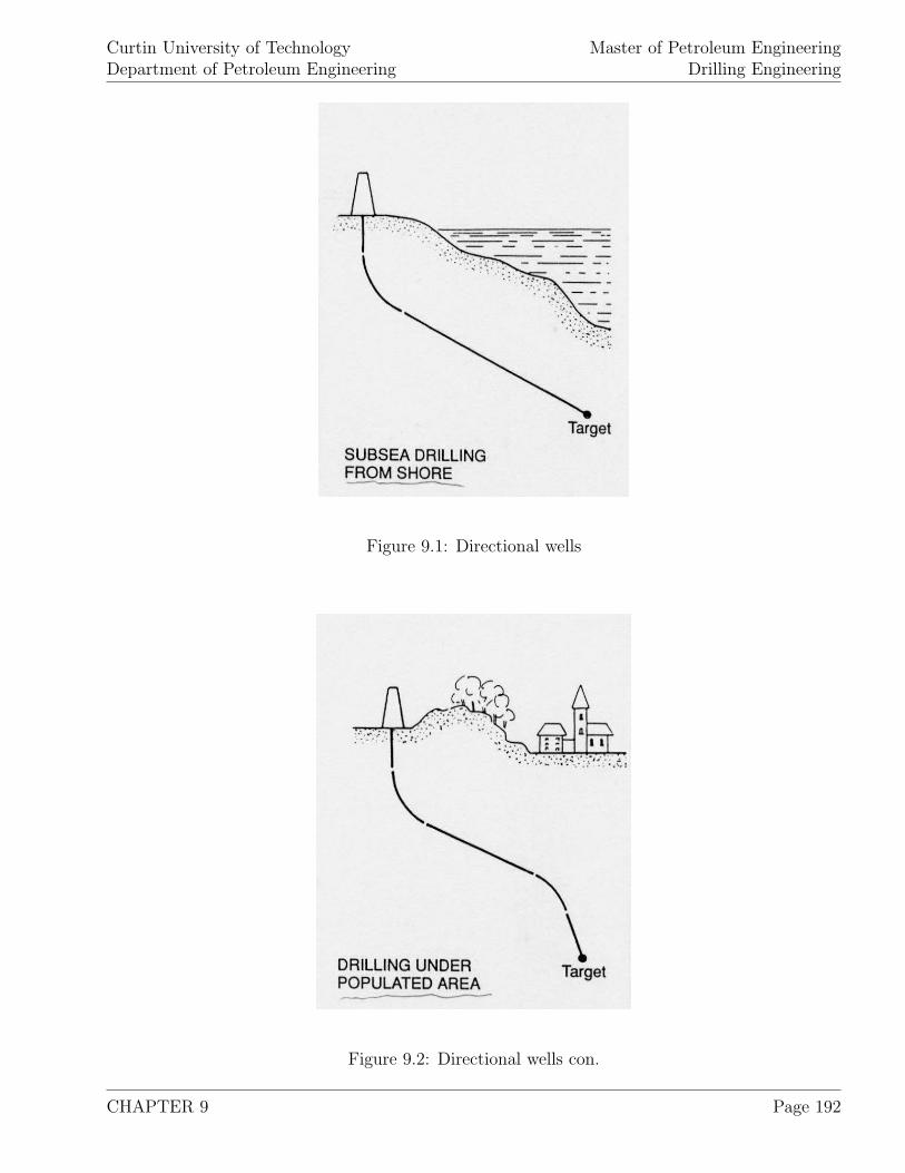
Curtin University of TechnologyDepartment of Petroleum Engineering
Master of Petroleum EngineeringDrilling Engineering
Figure 9.1: Directional wells
Figure 9.2: Directional wells con.
CHAPTER 9 Page 192
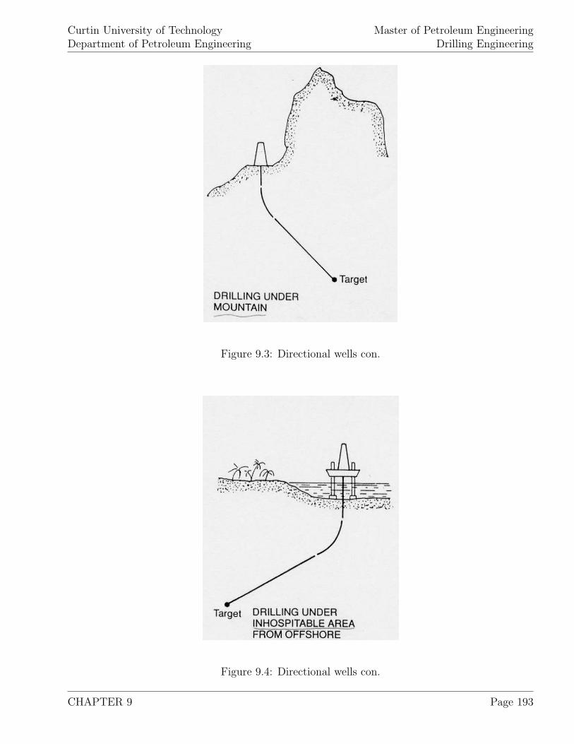
Curtin University of TechnologyDepartment of Petroleum Engineering
Master of Petroleum EngineeringDrilling Engineering
Figure 9.3: Directional wells con.
Figure 9.4: Directional wells con.
CHAPTER 9 Page 193
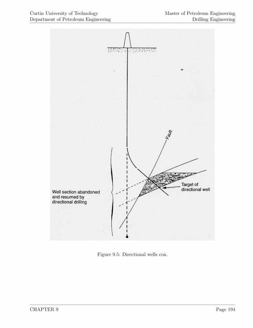
Curtin University of TechnologyDepartment of Petroleum Engineering
Master of Petroleum EngineeringDrilling Engineering
Figure 9.5: Directional wells con.
CHAPTER 9 Page 194
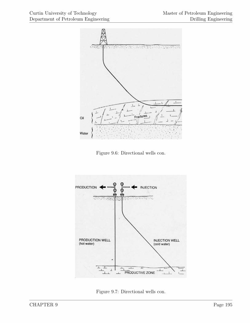
Curtin University of TechnologyDepartment of Petroleum Engineering
Master of Petroleum EngineeringDrilling Engineering
Figure 9.6: Directional wells con.
Figure 9.7: Directional wells con.
CHAPTER 9 Page 195
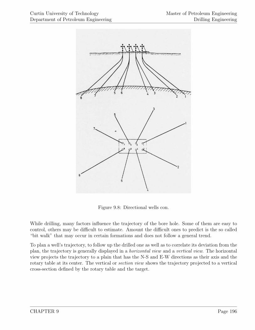
Curtin University of TechnologyDepartment of Petroleum Engineering
Master of Petroleum EngineeringDrilling Engineering
Figure 9.8: Directional wells con.
While drilling, many factors influence the trajectory of the bore hole. Some of them are easy tocontrol, others may be difficult to estimate. Amount the difficult ones to predict is the so called“bit walk” that may occur in certain formations and does not follow a general trend.
To plan a well’s trajectory, to follow up the drilled one as well as to correlate its deviation from theplan, the trajectory is generally displayed in a horizontal view and a vertical view. The horizontalview projects the trajectory to a plain that has the N-S and E-W directions as their axis and therotary table at its center. The vertical or section view shows the trajectory projected to a verticalcross-section defined by the rotary table and the target.
CHAPTER 9 Page 196
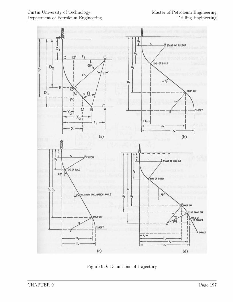
Curtin University of TechnologyDepartment of Petroleum Engineering
Master of Petroleum EngineeringDrilling Engineering
Figure 9.9: Definitions of trajectory
CHAPTER 9 Page 197
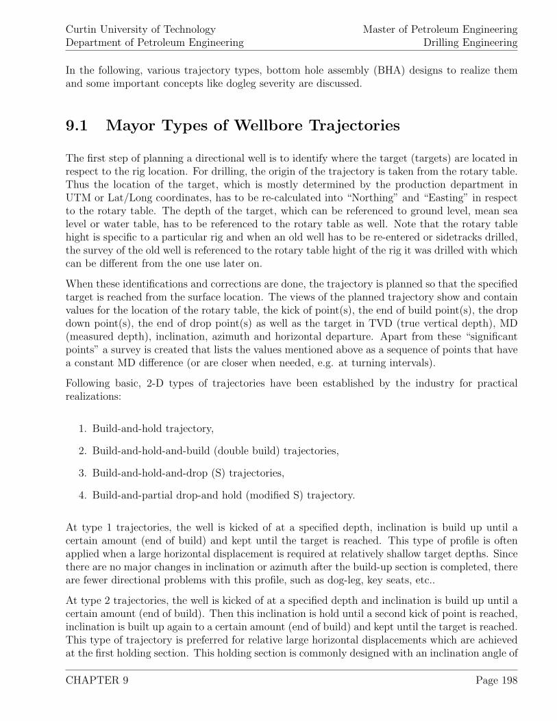
Curtin University of TechnologyDepartment of Petroleum Engineering
Master of Petroleum EngineeringDrilling Engineering
In the following, various trajectory types, bottom hole assembly (BHA) designs to realize themand some important concepts like dogleg severity are discussed.
9.1 Mayor Types of Wellbore Trajectories
The first step of planning a directional well is to identify where the target (targets) are located inrespect to the rig location. For drilling, the origin of the trajectory is taken from the rotary table.Thus the location of the target, which is mostly determined by the production department inUTM or Lat/Long coordinates, has to be re-calculated into “Northing” and “Easting” in respectto the rotary table. The depth of the target, which can be referenced to ground level, mean sealevel or water table, has to be referenced to the rotary table as well. Note that the rotary tablehight is specific to a particular rig and when an old well has to be re-entered or sidetracks drilled,the survey of the old well is referenced to the rotary table hight of the rig it was drilled with whichcan be different from the one use later on.
When these identifications and corrections are done, the trajectory is planned so that the specifiedtarget is reached from the surface location. The views of the planned trajectory show and containvalues for the location of the rotary table, the kick of point(s), the end of build point(s), the dropdown point(s), the end of drop point(s) as well as the target in TVD (true vertical depth), MD(measured depth), inclination, azimuth and horizontal departure. Apart from these “significantpoints” a survey is created that lists the values mentioned above as a sequence of points that havea constant MD difference (or are closer when needed, e.g. at turning intervals).
Following basic, 2-D types of trajectories have been established by the industry for practicalrealizations:
1. Build-and-hold trajectory,
2. Build-and-hold-and-build (double build) trajectories,
3. Build-and-hold-and-drop (S) trajectories,
4. Build-and-partial drop-and hold (modified S) trajectory.
At type 1 trajectories, the well is kicked of at a specified depth, inclination is build up until acertain amount (end of build) and kept until the target is reached. This type of profile is oftenapplied when a large horizontal displacement is required at relatively shallow target depths. Sincethere are no major changes in inclination or azimuth after the build-up section is completed, thereare fewer directional problems with this profile, such as dog-leg, key seats, etc..
At type 2 trajectories, the well is kicked of at a specified depth and inclination is build up until acertain amount (end of build). Then this inclination is hold until a second kick of point is reached,inclination is built up again to a certain amount (end of build) and kept until the target is reached.This type of trajectory is preferred for relative large horizontal displacements which are achievedat the first holding section. This holding section is commonly designed with an inclination angle of
CHAPTER 9 Page 198
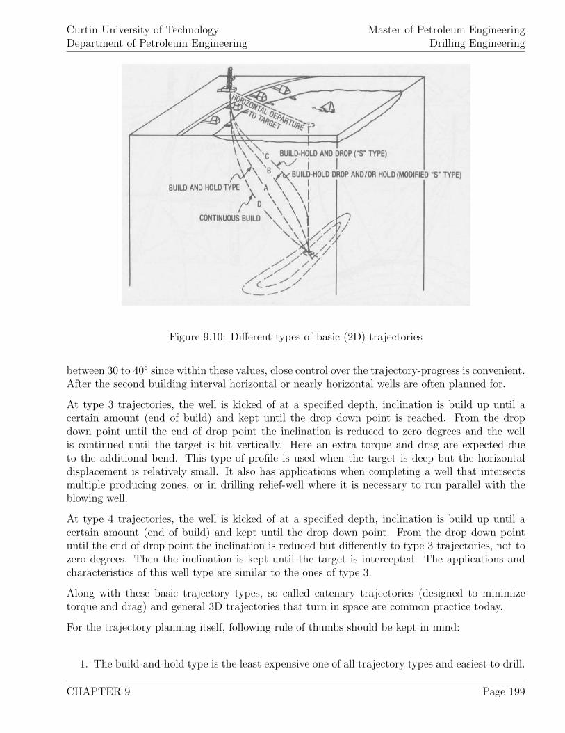
Curtin University of TechnologyDepartment of Petroleum Engineering
Master of Petroleum EngineeringDrilling Engineering
Figure 9.10: Different types of basic (2D) trajectories
between 30 to 40◦ since within these values, close control over the trajectory-progress is convenient.After the second building interval horizontal or nearly horizontal wells are often planned for.
At type 3 trajectories, the well is kicked of at a specified depth, inclination is build up until acertain amount (end of build) and kept until the drop down point is reached. From the dropdown point until the end of drop point the inclination is reduced to zero degrees and the wellis continued until the target is hit vertically. Here an extra torque and drag are expected dueto the additional bend. This type of profile is used when the target is deep but the horizontaldisplacement is relatively small. It also has applications when completing a well that intersectsmultiple producing zones, or in drilling relief-well where it is necessary to run parallel with theblowing well.
At type 4 trajectories, the well is kicked of at a specified depth, inclination is build up until acertain amount (end of build) and kept until the drop down point. From the drop down pointuntil the end of drop point the inclination is reduced but differently to type 3 trajectories, not tozero degrees. Then the inclination is kept until the target is intercepted. The applications andcharacteristics of this well type are similar to the ones of type 3.
Along with these basic trajectory types, so called catenary trajectories (designed to minimizetorque and drag) and general 3D trajectories that turn in space are common practice today.
For the trajectory planning itself, following rule of thumbs should be kept in mind:
1. The build-and-hold type is the least expensive one of all trajectory types and easiest to drill.
CHAPTER 9 Page 199
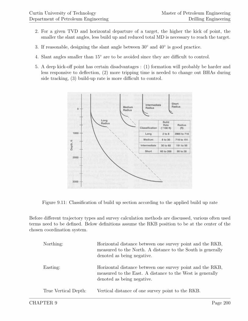
Curtin University of TechnologyDepartment of Petroleum Engineering
Master of Petroleum EngineeringDrilling Engineering
2. For a given TVD and horizontal departure of a target, the higher the kick of point, thesmaller the slant angles, less build up and reduced total MD is necessary to reach the target.
3. If reasonable, designing the slant angle between 30◦ and 40◦ is good practice.
4. Slant angles smaller than 15◦ are to be avoided since they are difficult to control.
5. A deep kick-off point has certain disadvantages : (1) formation will probably be harder andless responsive to deflection, (2) more tripping time is needed to change out BHAs duringside tracking, (3) build-up rate is more difficult to control.
Figure 9.11: Classification of build up section according to the applied build up rate
Before different trajectory types and survey calculation methods are discussed, various often usedterms need to be defined. Below definitions assume the RKB position to be at the center of thechosen coordination system.
Northing: Horizontal distance between one survey point and the RKB,measured to the North. A distance to the South is generallydenoted as being negative.
Easting: Horizontal distance between one survey point and the RKB,measured to the East. A distance to the West is generallydenoted as being negative.
True Vertical Depth: Vertical distance of one survey point to the RKB.
CHAPTER 9 Page 200
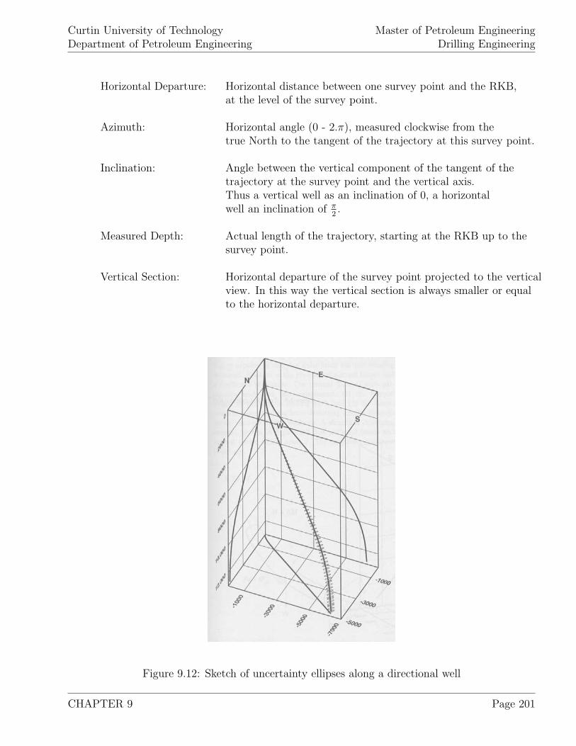
Curtin University of TechnologyDepartment of Petroleum Engineering
Master of Petroleum EngineeringDrilling Engineering
Horizontal Departure: Horizontal distance between one survey point and the RKB,at the level of the survey point.
Azimuth: Horizontal angle (0 - 2.π), measured clockwise from thetrue North to the tangent of the trajectory at this survey point.
Inclination: Angle between the vertical component of the tangent of thetrajectory at the survey point and the vertical axis.Thus a vertical well as an inclination of 0, a horizontalwell an inclination of π
2.
Measured Depth: Actual length of the trajectory, starting at the RKB up to thesurvey point.
Vertical Section: Horizontal departure of the survey point projected to the verticalview. In this way the vertical section is always smaller or equalto the horizontal departure.
Figure 9.12: Sketch of uncertainty ellipses along a directional well
CHAPTER 9 Page 201
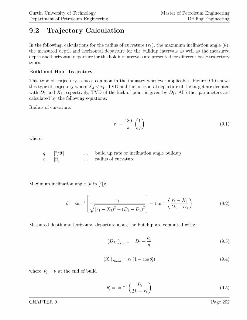
Curtin University of TechnologyDepartment of Petroleum Engineering
Master of Petroleum EngineeringDrilling Engineering
9.2 Trajectory Calculation
In the following, calculations for the radius of curvature (r1), the maximum inclination angle (θ),the measured depth and horizontal departure for the buildup intervals as well as the measureddepth and horizontal departure for the holding intervals are presented for different basic trajectorytypes.
Build-and-Hold Trajectory
This type of trajectory is most common in the industry whenever applicable. Figure 9.10 showsthis type of trajectory where X3 < r1. TVD and the horizontal departure of the target are denotedwith D3 and X3 respectively, TVD of the kick of point is given by D1. All other parameters arecalculated by the following equations:
Radius of curvature:
r1 =180
π.
(1
q
)(9.1)
where:
q [◦/ft] ... build up rate or inclination angle buildupr1 [ft] ... radius of curvature
Maximum inclination angle (θ in [◦]):
θ = sin−1
r1√
(r1 − X3)2 + (D3 − D1)
2
− tan−1
(r1 − X3
D3 − D1
)(9.2)
Measured depth and horizontal departure along the buildup are computed with:
(DMi)Build = D1 +
θ′iq
(9.3)
(Xi)Build = r1 (1 − cos θ′i) (9.4)
where, θ′i = θ at the end of build
θ′i = sin−1
(Di
D1 + r1
)(9.5)
CHAPTER 9 Page 202
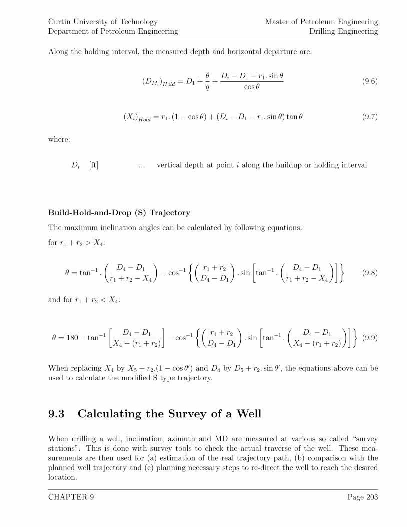
Curtin University of TechnologyDepartment of Petroleum Engineering
Master of Petroleum EngineeringDrilling Engineering
Along the holding interval, the measured depth and horizontal departure are:
(DMi)Hold = D1 +
θ
q+
Di − D1 − r1. sin θ
cos θ(9.6)
(Xi)Hold = r1. (1 − cos θ) + (Di − D1 − r1. sin θ) tan θ (9.7)
where:
Di [ft] ... vertical depth at point i along the buildup or holding interval
Build-Hold-and-Drop (S) Trajectory
The maximum inclination angles can be calculated by following equations:
for r1 + r2 > X4:
θ = tan−1 .
(D4 − D1
r1 + r2 − X4
)− cos−1
{(r1 + r2
D4 − D1
). sin
[tan−1 .
(D4 − D1
r1 + r2 − X4
)]}(9.8)
and for r1 + r2 < X4:
θ = 180− tan−1
[D4 − D1
X4 − (r1 + r2)
]− cos−1
{(r1 + r2
D4 − D1
). sin
[tan−1 .
(D4 − D1
X4 − (r1 + r2)
)]}(9.9)
When replacing X4 by X5 + r2.(1 − cos θ′) and D4 by D5 + r2. sin θ′, the equations above can beused to calculate the modified S type trajectory.
9.3 Calculating the Survey of a Well
When drilling a well, inclination, azimuth and MD are measured at various so called “surveystations”. This is done with survey tools to check the actual traverse of the well. These mea-surements are then used for (a) estimation of the real trajectory path, (b) comparison with theplanned well trajectory and (c) planning necessary steps to re-direct the well to reach the desiredlocation.
CHAPTER 9 Page 203
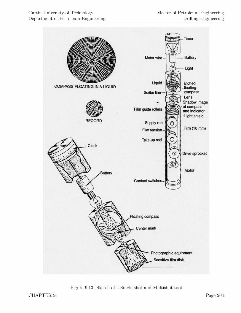
Curtin University of TechnologyDepartment of Petroleum Engineering
Master of Petroleum EngineeringDrilling Engineering
Figure 9.13: Sketch of a Single shot and Multishot tool
CHAPTER 9 Page 204
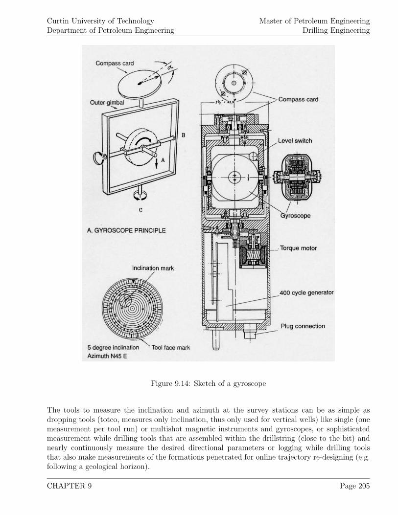
Curtin University of TechnologyDepartment of Petroleum Engineering
Master of Petroleum EngineeringDrilling Engineering
Figure 9.14: Sketch of a gyroscope
The tools to measure the inclination and azimuth at the survey stations can be as simple asdropping tools (totco, measures only inclination, thus only used for vertical wells) like single (onemeasurement per tool run) or multishot magnetic instruments and gyroscopes, or sophisticatedmeasurement while drilling tools that are assembled within the drillstring (close to the bit) andnearly continuously measure the desired directional parameters or logging while drilling toolsthat also make measurements of the formations penetrated for online trajectory re-designing (e.g.following a geological horizon).
CHAPTER 9 Page 205
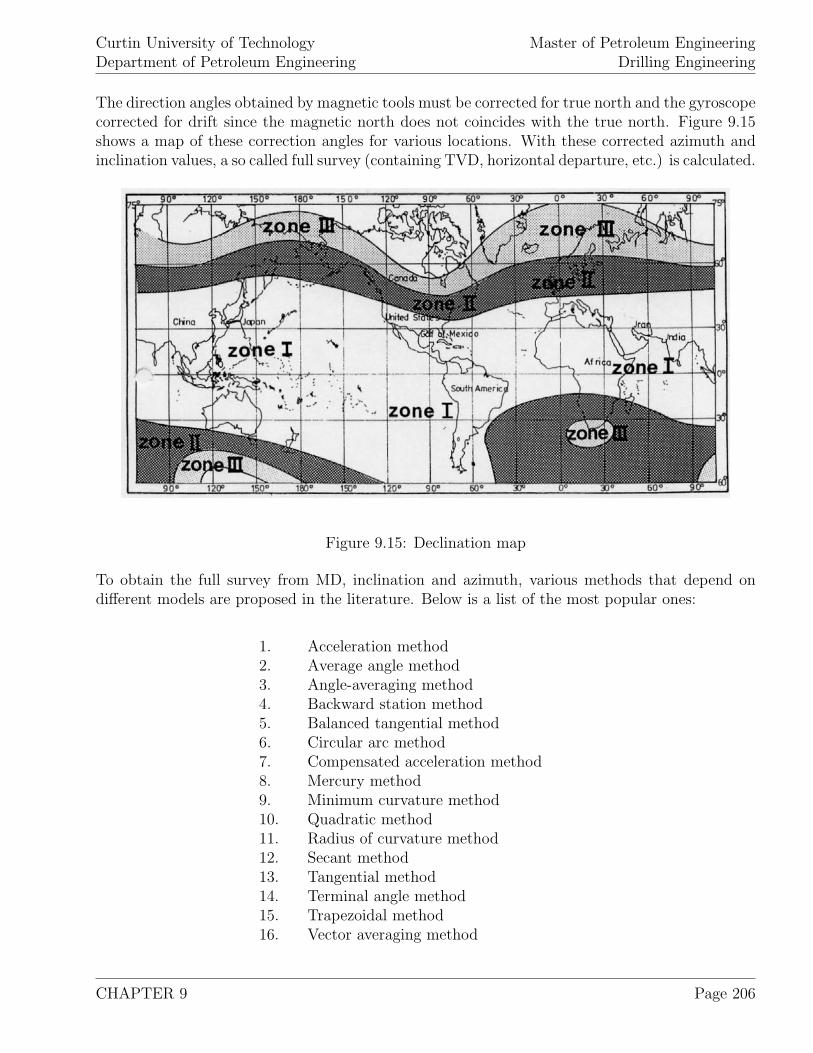
Curtin University of TechnologyDepartment of Petroleum Engineering
Master of Petroleum EngineeringDrilling Engineering
The direction angles obtained by magnetic tools must be corrected for true north and the gyroscopecorrected for drift since the magnetic north does not coincides with the true north. Figure 9.15shows a map of these correction angles for various locations. With these corrected azimuth andinclination values, a so called full survey (containing TVD, horizontal departure, etc.) is calculated.
Figure 9.15: Declination map
To obtain the full survey from MD, inclination and azimuth, various methods that depend ondifferent models are proposed in the literature. Below is a list of the most popular ones:
1. Acceleration method2. Average angle method3. Angle-averaging method4. Backward station method5. Balanced tangential method6. Circular arc method7. Compensated acceleration method8. Mercury method9. Minimum curvature method10. Quadratic method11. Radius of curvature method12. Secant method13. Tangential method14. Terminal angle method15. Trapezoidal method16. Vector averaging method
CHAPTER 9 Page 206
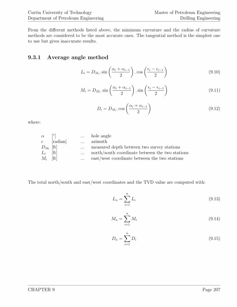
Curtin University of TechnologyDepartment of Petroleum Engineering
Master of Petroleum EngineeringDrilling Engineering
From the different methods listed above, the minimum curvature and the radius of curvaturemethods are considered to be the most accurate ones. The tangential method is the simplest oneto use but gives inaccurate results.
9.3.1 Average angle method
Li = DMi. sin
(αi + αi−1
2
). cos
(εi − εi−1
2
)(9.10)
Mi = DMi. sin
(αi + αi−1
2
). sin
(εi − εi−1
2
)(9.11)
Di = DMi. cos
(αi + αi−1
2
)(9.12)
where:
α [◦] ... hole angleε [radian] ... azimuthDMi
[ft] ... measured depth between two survey stationsLi [ft] ... north/south coordinate between the two stationsMi [ft] ... east/west coordinate between the two stations
The total north/south and east/west coordinates and the TVD value are computed with:
Ln =n∑
i=1
Li (9.13)
Mn =n∑
i=1
Mi (9.14)
Dn =n∑
i=1
Di (9.15)
CHAPTER 9 Page 207
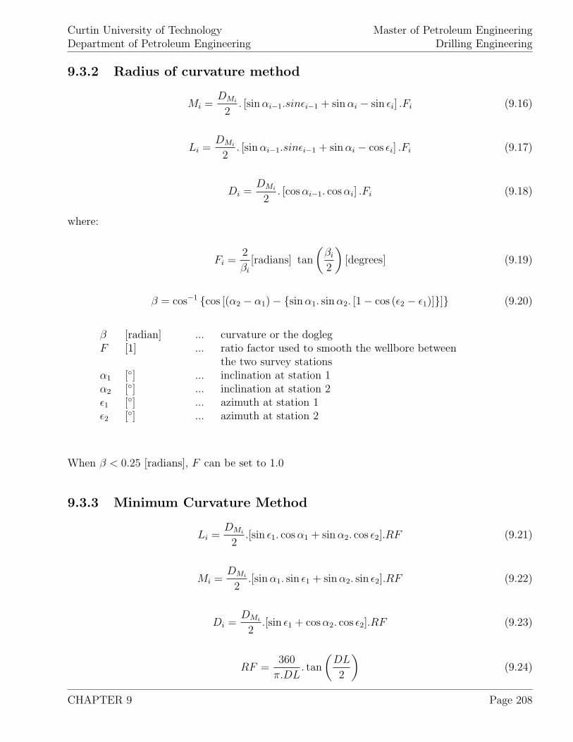
Curtin University of TechnologyDepartment of Petroleum Engineering
Master of Petroleum EngineeringDrilling Engineering
9.3.2 Radius of curvature method
Mi =DMi
2. [sin αi−1.sinεi−1 + sin αi − sin εi] .Fi (9.16)
Li =DMi
2. [sin αi−1.sinεi−1 + sin αi − cos εi] .Fi (9.17)
Di =DMi
2. [cos αi−1. cos αi] .Fi (9.18)
where:
Fi =2
βi
[radians] tan
(βi
2
)[degrees] (9.19)
β = cos−1 {cos [(α2 − α1) − {sin α1. sin α2. [1 − cos (ε2 − ε1)]}]} (9.20)
β [radian] ... curvature or the doglegF [1] ... ratio factor used to smooth the wellbore between
the two survey stationsα1 [◦] ... inclination at station 1α2 [◦] ... inclination at station 2ε1 [◦] ... azimuth at station 1ε2 [◦] ... azimuth at station 2
When β < 0.25 [radians], F can be set to 1.0
9.3.3 Minimum Curvature Method
Li =DMi
2.[sin ε1. cos α1 + sin α2. cos ε2].RF (9.21)
Mi =DMi
2.[sin α1. sin ε1 + sin α2. sin ε2].RF (9.22)
Di =DMi
2.[sin ε1 + cos α2. cos ε2].RF (9.23)
RF =360
π.DL. tan
(DL
2
)(9.24)
CHAPTER 9 Page 208
Curtin University of TechnologyDepartment of Petroleum Engineering
Master of Petroleum EngineeringDrilling Engineering
cos(DL) = cos(α2 − α1) − sin α1. sin α2. (1 − cos(ε2 − ε1)) (9.25)
where:
DL [◦/100 ft] ... dog leg
9.4 Dogleg Severity Calculations
By definition, a dogleg is a sudden change of inclination and/or direction of a well’s trajectory.For description purpose, the change is usually expressed in a 100-[ft] interval ([◦/ 100 ft]) andcalled “dogleg severity”. As it has been seen in practice, large dogleg severities can lead to failureof drillpipe, drill collar or tool joints as well as create so called “keyseats” which result in stuckdrillstrings.
To obtain the dogleg severity, the survey calculated with one of the methods described above isused along with following equations:
β = 2. sin−1 .
√sin2
(∆α
2
)+ sin2
(∆ε
2
). sin2
(α + αN
2
)(9.26)
or:
β ≈ cos−1 (cos ∆ε. sin αN . sin α + cos α. cos αN) (9.27)
δ =β
Lc
.100 (9.28)
where:
δ [◦/100 ft] ... dogleg severityβ [◦] ... total angle of change (turn)αN [◦] ... new inclination∆ε [◦] ... change in azimuth∆α [◦] ... change in inclinationLc [ft] ... length over which change of trajectory occurs
Note: To reduce the wear-effect of large dogleg severities, the add of multiple steel or rubberdrillpipe protectors which are cylindrical pieces, having an outside diameter equal to the outsidediameter of the tool joints, have proven to be efficient.
CHAPTER 9 Page 209
Curtin University of TechnologyDepartment of Petroleum Engineering
Master of Petroleum EngineeringDrilling Engineering
9.5 Deflection Tools and Techniques
The methods presented above calculate the trajectory path of the well as it is drilled. The actualtrajectory is constantly compared with the planned one and in case the actual one is going of course(which it always does to some extend), correction steps to bring the trajectory on course again haveto be taken. To correct the course of the well in case of minor deflections, an experienced driller canvary the individual drilling parameters (WOB, RPM, etc.) to adjust for the of-going trajectory.In case the trajectory is largely of course, a deflection tool has to be run and drilling in slidingmode (e.g. positive displacement motor (PDM)) carried out to make the necessary correction. Todetermine the direction the well is drilled in sliding mode, the bottom hole assembly containingthe deflection tool is rotated from the surface by rotating the whole drill string. Then, either a socalled “Ragland vector diagram” or the following equations are applied to compute the tool faceorientation. The computational results have shown to be more accurate than the graphical onegained from the Ragland vector diagram. The tool face angle is given by:
γ = cos−1
(cos α. cos β − cos βN
sin α. sin β
)= sin−1
(sin αN . sin ∆ε
sin β
)(9.29)
The new inclination and direction angles are:
αN = cos−1 (cos α. cos β − sin α. sin β. cos γ) (9.30)
∆ε = tan−1
(tan β. tan γ
sin α + tan β. cos α. cos γ
)(9.31)
where for γ is right of high side of the borehole:
εN = ε + ∆ε (9.32)
and for γ is left of high side of the borehole:
εN = ε − ∆ε (9.33)
where:
εN [◦] ... new direction of the trajectoryαN [◦] ... new inclination of the trajectory
Although rotary assemblies can be designed to alter the path of the wellbore, there are certaincircumstances where it is necessary to use special deflection tools, for example kicking-off and
CHAPTER 9 Page 210
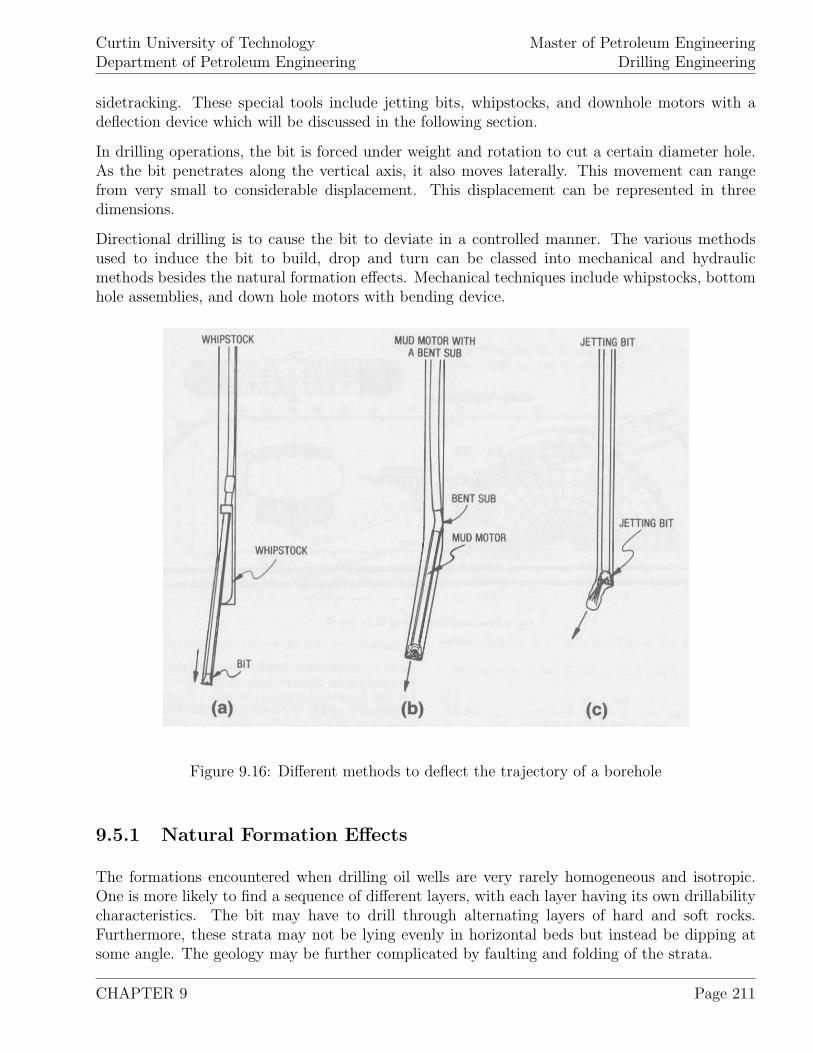
Curtin University of TechnologyDepartment of Petroleum Engineering
Master of Petroleum EngineeringDrilling Engineering
sidetracking. These special tools include jetting bits, whipstocks, and downhole motors with adeflection device which will be discussed in the following section.
In drilling operations, the bit is forced under weight and rotation to cut a certain diameter hole.As the bit penetrates along the vertical axis, it also moves laterally. This movement can rangefrom very small to considerable displacement. This displacement can be represented in threedimensions.
Directional drilling is to cause the bit to deviate in a controlled manner. The various methodsused to induce the bit to build, drop and turn can be classed into mechanical and hydraulicmethods besides the natural formation effects. Mechanical techniques include whipstocks, bottomhole assemblies, and down hole motors with bending device.
Figure 9.16: Different methods to deflect the trajectory of a borehole
9.5.1 Natural Formation Effects
The formations encountered when drilling oil wells are very rarely homogeneous and isotropic.One is more likely to find a sequence of different layers, with each layer having its own drillabilitycharacteristics. The bit may have to drill through alternating layers of hard and soft rocks.Furthermore, these strata may not be lying evenly in horizontal beds but instead be dipping atsome angle. The geology may be further complicated by faulting and folding of the strata.
CHAPTER 9 Page 211
Curtin University of TechnologyDepartment of Petroleum Engineering
Master of Petroleum EngineeringDrilling Engineering
As the bit drills across a formation boundary, it will tend to be deflected from its original course.Experience has shown that where the formations are steeply dipping (greater than about 60◦) thebit tends to drill parallel with the bedding planes. Where the formation dip is less steep, the bittends to drill at right angles to the bedding planes. In addition to changes in inclination theremay also be changes in direction in which case the bit will tend to walk. Under normal rotarydrilling, the bit will tend to walk to the right, but with a downhole motor the effect of reactivetorque may force it to the left. Drilling parameters such as: weight on bit, RPM, and hydraulics,will also affect the amount of deviation.
9.5.2 Hydraulic Method (Jetting)
This method of changing the trajectory of a wellbore requires the use of a jetting bit to washaway the formation. Water or drilling mud is pumped through a large jet that is oriented in thedirection of the desired trajectory change.
Jetting is a technique best suited to soft-medium formation in which the compressive strengthis relatively low and hydraulic power can be used to wash away a pocket of the formation toinitiate deflection. The amount of inclination produced is also related to the type of bottom holeassembly used with the jetting bits. There are two commercial bits especially designed for thejetting technique. One is a two-cone bit with an extended jet replacing the third cone and thesecond one is a conventional three cone bit with two small and one large “big eye” jet. The actualdesign of the jetting process is a function of hole size, pump capacity, expected formation hardness,and the desired bit cleaning efficiency while drilling.
Compared to trajectory deflection using a whipstock or downhole motors, jetting is the mostapproximate method. On any particular run, the bit is mounted on an assembly, which includesan orienting sub and a full-gauge stabilizer near the bit. Once the bit touches the bottom, the largenozzle is oriented in the required direction. Maximum circulation rate is used to begin washingwithout rotating the drill string. The pipe is worked up and down with continuous jetting, untila pocket is washed away. At this stage the drill string can be rotated to ream out the pocketand continue building angle as more weight is applied to the bit. Surveys are taken frequently toensure that the inclination and direction are correct.
Advantages of this method are: (1) several attempts can be made to initiate deflection withoutpulling out of the hole, (2) a full gauge hole can be drilled from the beginning.
Disadvantages of this method are: (1) the technique is limited to soft-medium formations,(2) severe dog-legs can occur if the jetting is not carefully controlled, (3) on smaller rigs there maynot be enough pump capacity to wash away the formation.
In summary, jetting is a very cost-efficient giving that kicking-off takes place under suitable geo-logical conditions. In general it requires a good directional monitoring.
CHAPTER 9 Page 212
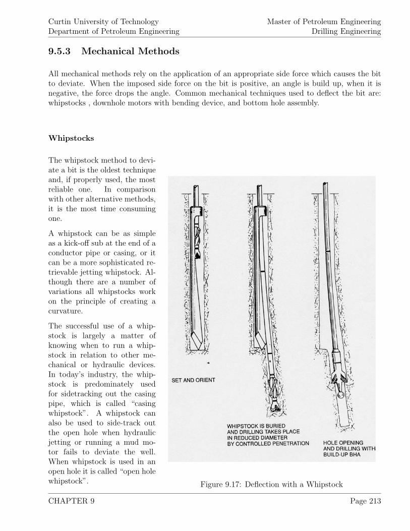
Curtin University of TechnologyDepartment of Petroleum Engineering
Master of Petroleum EngineeringDrilling Engineering
9.5.3 Mechanical Methods
All mechanical methods rely on the application of an appropriate side force which causes the bitto deviate. When the imposed side force on the bit is positive, an angle is build up, when it isnegative, the force drops the angle. Common mechanical techniques used to deflect the bit are:whipstocks , downhole motors with bending device, and bottom hole assembly.
Whipstocks
Figure 9.17: Deflection with a Whipstock
The whipstock method to devi-ate a bit is the oldest techniqueand, if properly used, the mostreliable one. In comparisonwith other alternative methods,it is the most time consumingone.
A whipstock can be as simpleas a kick-off sub at the end of aconductor pipe or casing, or itcan be a more sophisticated re-trievable jetting whipstock. Al-though there are a number ofvariations all whipstocks workon the principle of creating acurvature.
The successful use of a whip-stock is largely a matter ofknowing when to run a whip-stock in relation to other me-chanical or hydraulic devices.In today’s industry, the whip-stock is predominately usedfor sidetracking out the casingpipe, which is called “casingwhipstock”. A whipstock canalso be used to side-track outthe open hole when hydraulicjetting or running a mud mo-tor fails to deviate the well.When whipstock is used in anopen hole it is called “open holewhipstock”.
CHAPTER 9 Page 213
Curtin University of TechnologyDepartment of Petroleum Engineering
Master of Petroleum EngineeringDrilling Engineering
A whipstock can be described as a steel wedge with a chisel shaped point at the bottom. Thischisel shape prevents the whipstock from turning when drilling begins. The whipstock, that isrun down hole, is attached to the lower end of the drill string by means of a shear pin. It is eitherset on the bottom or anchored and locked in a packer which was previously installed in a casingstring.
A modern whipstock has a tapered concave groove, called the tool face, which helps in orientingthe whipstock. Once it is installed down hole, it guides the bit or the mill against the casing orthe open hole wall to drill in the desired direction.
Open Hole Whipstock Running Procedures
The procedures for running the whipstock can be summarized as follows:
1. A whipstock is to be selected according to the wedge needed to effect the desired deflection.
2. A bit that is small enough to fit in the hole with the chosen whipstock is selected.
3. The whipstock is attached to the bottom of the drillstring by means of a shear pin.
4. Having run into the hole, the drillstring is rotated according to the survey information, untilthe tool-face of the whipstock is oriented in the desired direction.
5. By applying enough weight, the chisel point is set firmly into the formation or cement plugto prevent the whipstock from rotating.
6. Additional weight is applied to shear the pin that holds the drill collar to the wedge. Rotationcan then begin.
7. A small diameter pilot hole is drilled to a depth of about 15 [ft] below the toe of the whipstockat which point the whipstock-stop reaches the top collar of the whipstock.
8. The pilot hole is then surveyed to make sure that it has been drilled in the right direction.
9. After the pilot hole has been surveyed, the bit and the whipstock are tripped out.
10. A hole opener is then run to ream out the pilot hole to the full size hole.
Casing Whipstock Running Procedures
The running steps for a casing whipstock can be summarized as:
1. The casing whipstock packer with anchor device is run to the kick-off point.
2. The alignment key is oriented using a gyro survey, so that the whipstock will land in aunique position, where the side track is needed.
CHAPTER 9 Page 214
Curtin University of TechnologyDepartment of Petroleum Engineering
Master of Petroleum EngineeringDrilling Engineering
3. The casing packer is set to provide a base for the whipstock.
4. The whipstock is attached to a starting mill by means of a shear pin and run in hole.
5. The whipstock is landed in the pre-oriented packer by means of a lock-sub (mule-shoestinger), and thereby oriented in the desired direction.
6. Weight is applied to break the shear pin thereby freeing the starting mill off the whipstock.The string is then rotated to mill the casing to create the window.
7. Once the window has been cut, the mill is replaced by a smaller sidetracking bit which isforced by the whipstock through the window outside the casing. A pilot hole can then bedrilled.
8. After drilling the pilot hole, the bottom hole assembly is pulled out and replaced by anassembly of string and watermelon mills to make the window large enough to accommodatea conventional bottom hole assembly.
The whipstock’s biggest advantage is that it provides a controlled hole curvature at the onset,while distributing the side force over the length of the whipstock body. Whipstocks can also berun at any depth in any kind of rock although they are best suited for use in very hard rock wherejetting and mud motor deflecting techniques are generally ineffective.
The main disadvantage of the whipstock is the necessity to drill the pilot hole and then trip outto change the smaller bit to one of the wellbore diameter.
Downhole Motor With Bending Device
The most common deflection technique currently in use involves running a downhole motor whichdrives the bit without rotating the drill string. Two different types of downhole motors have beendeveloped, the positive displacement mud motor and the mud turbine. To create a change in thetrajectory, downhole motors require a deflection device. The deflection is provided either by aspecial sub placed above the motor, called a bent sub, or by introducing a deflection at the bottomsection or below the motor. The latter is known as steerable bottom hole assembly.
Bent Sub
A bent sub is about two feet long having the axis of the lower pin connection machined slightlyoff vertical. The amount of this so called “offset angle” varies between 0.5 and 3.0◦. The directionin which the tool is deflected, called “tool face”, is marked by a reference line on the outer surfaceof the sub. The bent sub itself is connected to a motor below it and to an orienting sub above it.Once the assembly is run to the bottom of the hole, the bent sub is oriented using the orientingsub and a survey tool. After orientation, mud circulation is started which initiates the operationof the mud motor and drives the bit without rotating the drill string. The amount of deflection
CHAPTER 9 Page 215
Curtin University of TechnologyDepartment of Petroleum Engineering
Master of Petroleum EngineeringDrilling Engineering
produced is mainly a function of the offset, the length and stiffness of the motor, and the hardnessof the formation.
Typically, this type of assembly is engaged in drilling until the hole inclination reaches about 20◦.At this point the motor and the bent sub are pulled out of the hole, and the building rotaryassembly is engaged to complete the building section of the hole.
Steerable Bottom Hole Assembly
The increased application of downhole motors and turbines as deflection tools has led to theconcept of having an adjustable component with the bottom hole assembly that is capable ofaltering the well path without having to pull out of the hole in order to change the bottom holeassembly. Such a steerable drilling system is comprised of a bit, a steerable motor, MWD toolsand stabilizing unit(s).
The three categories of commercially available steerable systems are: (1) adjustable bent subabove the motor, (2) motor housing with one or two bends, and (3) offset stabilizer on motor.
1. Adjustable bent sub above motor: The conventional bent subs with fixed angle have thedisadvantage that they cannot be run in the hole in a straight position coaxial to the string axisand therefore, cannot be used in rotary drilling. Thus, the advantage of a down hole adjustabledeflection device is that it can be run in the hole coaxially and the required amount of deflectioncan be controlled from the surface. This makes directional drilling more efficient and less timeconsuming.
The multi-angle bent-sub associated with a downhole motor allows for drilling of the completebuild up zone and of the constant angle zone with the same bottom hole assembly. Here the bentsub angle is controlled from the surface.
The adjustable bent sub consists of an upper and a lower sub that are connected by an offsetconical swiveling joint. The axis of the conical joint is tilted with respect to the main axis of thetool. The lower sub is constructed so that it is able to rotate at an angle that is slightly offsetfrom the vertical axis. Initially the tool is made up so that the upper and the lower subs arealigned. When the lower sub is rotated it becomes locked in such a position that the two subsare offset by a small amount, thereby forming a bend in the BHA. Further rotation increases thesize of the bend. The size of the bend reaches maximum when half revolution is made after fiveactuations. Further rotation decreases the angle gradually back to the straight position after fivemore actuations to make a complete revolution.
The lower sub has ten possible positions to adopt and it actuates from one position to the next bya hydraulic device. The actuator creates a temporary surge of pressure that is transmitted to ashaft that turns the lower sub. At the end of the pressure surge, the lower sub is locked into thatposition until the next surge. The drill string must be lifted off bottom while changing the angleof the bent sub. Flow rate is adjusted to provide the necessary increase in pressure to actuate thetool. Once in position, the mud pump is shut down and the lower sub is locked into this position.It is therefore, possible to operate the tool remotely from the rig floor.
CHAPTER 9 Page 216
Curtin University of TechnologyDepartment of Petroleum Engineering
Master of Petroleum EngineeringDrilling Engineering
2. Motor housing with one or two bends: when the deflecting device is placed on the topof a downhole motor, it introduces the deflection at a distance far enough from the bit to createa considerable bit offset. The amount of bit offset introduced by the bent subs prohibits rotatingof the drill-string. Under this circumstance drilling proceeds in sliding or orienting mode only.
Building a bent house at the lower end of a positive displacement motor itself introduces a deflec-tion which is much closer to the bit and therefore, more effective than what is possible with thebent sub on the top of the motor. This means that a bent housing will provide a larger turn thana bent sub of similar size and deflection.
The bent housing motor assembly can be used in steering mode as well as in rotary mode becausethe initial bit side loading created by the small bit offset rotates with the drilling string therebynegating its deviating effect.
The bit offset in the bent house assembly can be reduced further without affecting the bit tilt angleby introducing a second tilt in the opposite direction to the first one. Here the body of the motoris brought back into a position aligning with the borehole axis. When the rotary table is engagedwhile the downhole motor is in the hole, bit offset is negated and the assembly drills straightahead to maintain inclination and direction. Such a deflecting unit is known as double-tilteduniversal joint housing (DTU). The DTU joint housing develops a minimum bit offset to give thenavigation drilling system a full steering capability. A bit angle of 0.25 to 0.78◦ is adequate toprovide directional control using the DTU.
The rotation of the bending motor housing for straight hole drilling causes a slightly over gaugedhole and that creates a “step” when the drilling switches from rotary to orient mode or vice versa.Therefore, the smaller the bit offset, the less the bit will cut with its side, and the smaller thesize of the step. Cutting with the bit face extends bit life and optimizes the rate of penetration.Similarly, by keeping the motor concentric to the hole, rotary drilling proceeds smoothly withoutexcessive rotational bending to the assembly.
A limitation with all steerable systems is that the stabilizers hang on to the hole wall at a step,and hence reduce the weight on bit. Although this step can happen with a conventional rotaryassembly, it is more common with steerable systems because the diameter of the hole drilled inrotary mode is slightly larger than the part drilled in orienting mood. The magnitude of this stepdepends on the formation hardness, stability and the build rate of the system. To minimize thestep problem, the near bit stabilizer should be under-gauged and should have shallow nose heelangles. The step size can be further reduced by minimizing the build rate of the system.
3. Offset Stabilizer on Motor: The positive displacement motor can use either a bent subabove the motor or have the housing (bend housing) below it. Mud turbines are restricted to theuse of the bent sub where the design of the turbine prohibits manufacture of a bent housing.
The deflection below the turbine is provided by a special stabilizer with an under-gauge blade,known as offset stabilizer, and is located on the turbine near the bit. The under-gauge blade isconsidered to be the tool face. It is oriented in the same way as the bent sub and the bent house.When the drill-string is not rotated, the turbine drives the bit along a predefined course which isgiven by the under-gauge blade orientation.
CHAPTER 9 Page 217
Curtin University of TechnologyDepartment of Petroleum Engineering
Master of Petroleum EngineeringDrilling Engineering
The greater the stabilizer offset (higher under-gauge blade), the greater the rate of build, but theamount of offset is limited.
Once the wellbore is brought back onto the planned trajectory, the drillstring can be rotated.Rotating the offset stabilizer results in a slightly over-gauge hole.
9.6 While Drilling Techniques
With “while drilling techniques”, the direction of the wellbore, condition of the drillstring as wellas the formations that have been penetrated can be measured and the measurements transferredto the rig-site while drilling. While drilling sensors are typically mounted at the BHA as closeas possible to the bit. Depending on the drillstring configuration, the distance between the bitand the measuring devices can be as little as 10 [ft]. In this way, the measurements taken aresomewhat behind the bit and depending on the penetration rate, are recorded with some lag-time.While drilling systems generally consist of (a) a power system, (b) measuring sensors and (c) atelemetry system for data transfer. The power system can be either based on a battery, a turbineor a combination of them. Batteries have the advantage that no circulation is needed to carry outmeasurements, thus while tripping, control logs can be run.
9.6.1 Measurement While Drilling
The term “measurement while drilling” (MWD) refers to the while drilling measurement of di-rectional parameters (MD, inclination, azimuth) as well as certain drilling parameters like WOB,downhole torque, temperature, etc. The sensor to perform these measurements are three orthogo-nal fluxgate magnetometers and three accelerometers. The use of gyroscope navigated MWD offerssignificant benefits over navigation sensors. They offer greater accuracy and are not susceptibleto inference from magnetic fields.
The drilling parameters measured with MWD tools are aimed to increase the drilling efficiency(stick-slip), be applied to detect abnormal formation pressures or any kind of hole problems.
Most MWD tools can operate at tool-temperatures up to 150 ◦C, some sensor work up to 175 ◦C.It should be noted that the tool-temperatures are generally about 20 ◦C less than the formationtemperatures, measured by wireline logs which is caused by the cooling effect of mud circulation.
Downhole pressures create less problems for MWD tools than downhole temperatures. Most MWDtools are designed to withstand up to 20,000 [psi] which is rarely encountered.
MWD tools are most sensitive to shock and vibrations. Torsional shock, created by stick-slip havebeen found to be able to cause tool failure, lateral shocks which can be magnitudes higher thanaxial shocks, can be reduced by the use of jars.
Normally sensors measure MWD shock loads constantly and transmit them to the rick. There thedriller can manipulate the drilling parameters to keep them in acceptable limits.
CHAPTER 9 Page 218
Curtin University of TechnologyDepartment of Petroleum Engineering
Master of Petroleum EngineeringDrilling Engineering
9.6.2 Logging While Drilling
The term “logging while drilling” (LWD) refers to the while drilling measurements of wirelineequivalent parameters like resistivity, porosity, density and sonic logs. When these parameters areknown, “geosteering” can be performed where the trajectory of the well is “re-designed” accordingto the actual formation’s position and shape.
9.6.3 Data Transfer
Since the amount of data measured by while drilling techniques can be large, mostly not allmeasurements are continuously transferred to the rig. Data that are not transferred are commonlystored and retrieved at the following trip. Several different systems have been developed to transferthe measured data to the surface, the “mud pulse telemetry” is the by far most often applied on.Three different mud pulse systems are commercially available today:
1. Positive pulse system: creates a momentary flow restriction (higher pressure than the drillingmud volume) in the drillpipe.
2. Negative pulse system: creates a pressure pulse lower than that of the mud volume byventing a small amount of high pressure drillstring mud from the drillpipe of the annulus.
3. Continuous wave system: creates a carrier frequency that is transmitted through the mudand encoded data using phase shifts of the carrier.
From the systems listed above, the positive pulse telemetry is the most often applied one since itis easiest to achieve even for extended reach wells.
When the signals reach the surface, they are retrieved by transducers that are located on thestandpipe and send to computers at the site for further evaluation.
The data transmitted are overlayed with noise where the mud pumps are the main source. Otherparameters that influence the “signal to noise range” are: what mud type and bit type are in use,the length of the well and the drilling parameters applied itself.
CHAPTER 9 Page 219
Curtin University of TechnologyDepartment of Petroleum Engineering
Master of Petroleum EngineeringDrilling Engineering
9.7 Examples
1. Calculate a build-and-hold trajectory to reach a target at 10,000 [ft] TVD and 2,600 [ft]horizontal departure. The kick off point shall be set to 1,500 [ft] and a build rate of 2 [◦/ 100ft] applied. Compute the: radius of curvature, maximum inclination angle, measured depth andhorizontal departure at the end of build as well as the measured depth and horizontal departureat 8,000 [ft].
2. When the inclination has changed from 5◦ to 7◦ together with a change of direction from N90Eto S82E over an interval of 75 [ft], what is the dogleg severity?
3. After going of course the trajectory has to be changed in inclination from 4◦ to 6◦ as well asin direction from 15◦ to 35◦ over the next 70 [ft], what is the tool-face setting and the expecteddogleg severity?
CHAPTER 9 Page 220
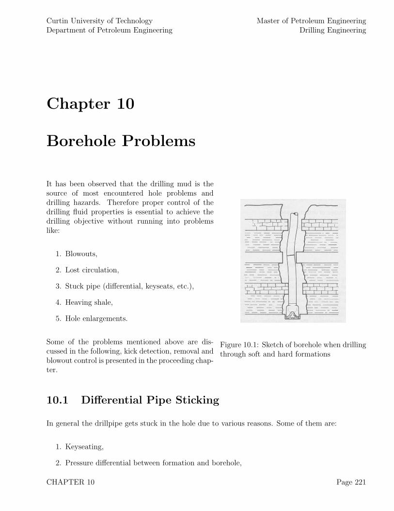
Curtin University of TechnologyDepartment of Petroleum Engineering
Master of Petroleum EngineeringDrilling Engineering
Chapter 10
Borehole Problems
Figure 10.1: Sketch of borehole when drillingthrough soft and hard formations
It has been observed that the drilling mud is thesource of most encountered hole problems anddrilling hazards. Therefore proper control of thedrilling fluid properties is essential to achieve thedrilling objective without running into problemslike:
1. Blowouts,
2. Lost circulation,
3. Stuck pipe (differential, keyseats, etc.),
4. Heaving shale,
5. Hole enlargements.
Some of the problems mentioned above are dis-cussed in the following, kick detection, removal andblowout control is presented in the proceeding chap-ter.
10.1 Differential Pipe Sticking
In general the drillpipe gets stuck in the hole due to various reasons. Some of them are:
1. Keyseating,
2. Pressure differential between formation and borehole,
CHAPTER 10 Page 221

Curtin University of TechnologyDepartment of Petroleum Engineering
Master of Petroleum EngineeringDrilling Engineering
3. Bit and drill collar balling,
4. Foreign objects or junk in the borehole,
5. Sloughing formations (heaving shales),
6. Improper solids removal leaving cuttings above the bit or drill collar.
A drillstring is called differential stuck when it is motionless and forced against a permeable for-mation (mud cake) due to excessive differential pressure (overbalance). In this situation, sketchedin figure 10.2, a section of the drillstring is pressed into the mud cake and literally glued to theborehole wall.
Figure 10.2: Differentially Stuck Drillstring
Danger of becoming differentially stuck is high when the drillstring is static in the hole for anextended time and thick mud cakes are present. It should be noted that the force that “glues”the drillstring on to the borehole wall and is given by equation 10.1, increases with time.
CHAPTER 10 Page 222
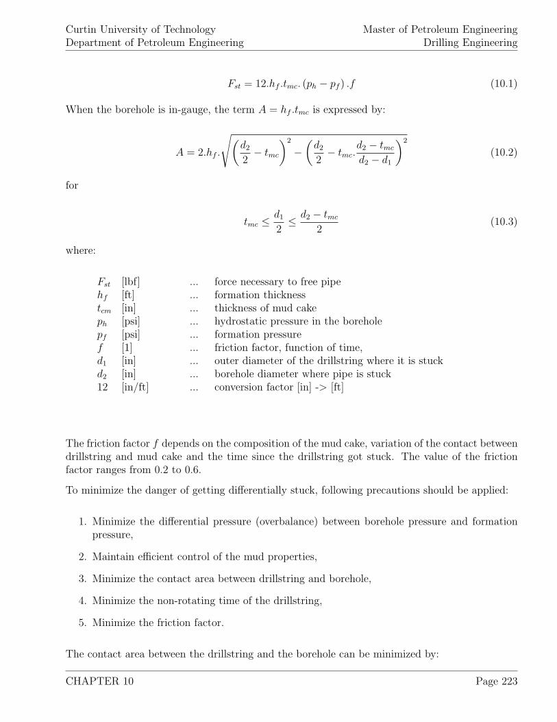
Curtin University of TechnologyDepartment of Petroleum Engineering
Master of Petroleum EngineeringDrilling Engineering
Fst = 12.hf .tmc. (ph − pf ) .f (10.1)
When the borehole is in-gauge, the term A = hf .tmc is expressed by:
A = 2.hf .
√(d2
2− tmc
)2
−(
d2
2− tmc.
d2 − tmc
d2 − d1
)2
(10.2)
for
tmc ≤ d1
2≤ d2 − tmc
2(10.3)
where:
Fst [lbf] ... force necessary to free pipehf [ft] ... formation thicknesstcm [in] ... thickness of mud cakeph [psi] ... hydrostatic pressure in the boreholepf [psi] ... formation pressuref [1] ... friction factor, function of time,d1 [in] ... outer diameter of the drillstring where it is stuckd2 [in] ... borehole diameter where pipe is stuck12 [in/ft] ... conversion factor [in] -> [ft]
The friction factor f depends on the composition of the mud cake, variation of the contact betweendrillstring and mud cake and the time since the drillstring got stuck. The value of the frictionfactor ranges from 0.2 to 0.6.
To minimize the danger of getting differentially stuck, following precautions should be applied:
1. Minimize the differential pressure (overbalance) between borehole pressure and formationpressure,
2. Maintain efficient control of the mud properties,
3. Minimize the contact area between drillstring and borehole,
4. Minimize the non-rotating time of the drillstring,
5. Minimize the friction factor.
The contact area between the drillstring and the borehole can be minimized by:
CHAPTER 10 Page 223
Curtin University of TechnologyDepartment of Petroleum Engineering
Master of Petroleum EngineeringDrilling Engineering
1. Using stabilizers on the drill collars,
2. Using grooved or noncircular drill collars,
3. Using drill collars with external upset,
4. Minimize filter cake thickness through proper design of the drilling mud.
The friction factor can be minimized by using low water-loss muds, oil-base muds and walnuthulls.
10.2 Free Point Calculation
In order to take actions to free the pipe, the knowledge of the depth where the drillstring is stuck,also called “free point”, is vital. Two methods are available to verify the free point location:(a) measurement of the drillstring stretch, measured at the surface when the string is pull with acertain amount of overpull and, (b) usage of so called “free point indicators”. Free point indicators,which are either strain gauge probes or subsurface probes, are special gauge tools that measurethe strain in the drillstring.
To compute the free point based on the drillpipe stretch, only measurements taken at the derrickare required. The procedure is summarized as:
1. Pulling the drillstring with normal hook load and mark a reference point X1 on the pipe.
2. Pull the drillstring with additional 20,000 to 40,000 [lbf], a force F that causes a stretch ofthe free portion of the drillstring. At the reference point-level, mark the drill pipe for X2.The stretch in [in] is given by X2−X1. Note that the applied overpull force must not exceedthe yield strength of the pipe or the joints.
3. Use equation 10.4 to compute the free point location:
Lst =735, 294. (X2 − X1) .Wdp
F(10.4)
where:
Lst [ft] ... length of free portion of the pipe, depth of free pointWdp [lb/ft] ... nominal weight of drillpipeF [lbf] ... additional force (overpull)
As it can be seen, equation 10.4 accounts for the stretch of the drillpipe only.
CHAPTER 10 Page 224
Curtin University of TechnologyDepartment of Petroleum Engineering
Master of Petroleum EngineeringDrilling Engineering
10.3 Freeing Differentially Stuck Pipe
When the location of the free point is verified, following methods to free the drillstring are possibleand should be tried in the order they are listed below.
10.3.1 Spotting Organic Fluids
A mixture of diesel and surfactants is pumped to the location where the drillstring is stuck. Thisis performed by pumping the mixture through the drillstring and up the annulus to the free pointdepth. Since the mixture is meant to reduce the thickness of the mud cake and the friction factor,sufficient time has to be allowed so that the mixture can be dissolved and the mud cake destroyed.While spotting, the drillstring is worked continuously to free the drillstring.
10.3.2 Hydrostatic Pressure Reduction
This method aims to create a pressure differential between the inside of the drillpipe and theannulus by pumping lower density fluid into the drillpipe. Since the hydrostatic pressure fromthe fluid inside the drillpipe and from the annulus have to be the same at the bottom of the hole,the mud level at the annulus as well as the pressure at the free point are reduced. The amountof low density fluid to be pumped into the drillstring and the resulting maximum drillpipe gaugepressures are given by:
Vo =Lst.Vdp
ρm − ρo
.
(ρm − pp
0.052.Lst
).
[1 +
Van
Vdp
.
(1 − ρo
ρm
)](10.5)
(pdp)max = 0.052.Vo
Vdp
. (ρm − ρo) (10.6)
The fluid level drop in the annulus [ft] can be computed with:
∆FL = Lst − pp
0.052.ρm
(10.7)
The equivalent mud weight during this bleed-off procedure is found as:
ρe = ρm − (pdp)max − pdp
0.052.Lst.[(
1 + Van
Vdp
).(1 − ρo
ρm
)] (10.8)
where:
Vdp [bbl/ft] ... capacity of drillpipe
CHAPTER 10 Page 225
Curtin University of TechnologyDepartment of Petroleum Engineering
Master of Petroleum EngineeringDrilling Engineering
Van [bbl/ft] ... capacity of annuluspp [psi] ... pore pressurepdp [psi] ... pressure within the drillpipe,
measured at the surface(pdp)max [psi] ... maximum drillpipe pressureρm [ppg] ... mud densityρo [ppg] ... density of fluid pumped downVo [bbl] ... volume of the fluid pumped downLst [ft] ... length of the drillstringD [ft] ... total depth of the well (MD)
It should be noted that precautions have to be taken that formations above the free point do notkick due to the pressure reduction of the annulus.
As alternative procedure to the method described above, the low density fluid can be pumpedinto both, the drillpipe and the annulus. Here the volumes of low density fluid required to reducethe differential pressure Vo and the volume of mud Vm required to pump behind the low densityfluid are determined by:
Vo = Van.pp
0.052− Lst.ρm
ρo − ρm
(10.9)
Vm = Vdp.Lst + Van. (D − Lst) (10.10)
10.3.3 Backoff Operations
When all attempts to free the stuck drillstring failed, backoff operations are the last alternative.By backoff operations parting the drillstring above the free point, recovering the free part of thedrillstring and fishing the remaining, stuck part of the string are understood.
Parting of the Drillstring
Nowadays four different methods are applied to part the drillstring:
1. Unscrew the pipe at a selective threaded joint above the stuck point using a prima cordexplosive run on a electric wireline.
2. Chemical cut - An electrical wireline tool and procedure that uses a propellant and a chem-ical, halogen fluoride, to burn a series of holes in the pipe thereby weakening it so that iteasily pulls apart with a slight pull.
CHAPTER 10 Page 226
Curtin University of TechnologyDepartment of Petroleum Engineering
Master of Petroleum EngineeringDrilling Engineering
3. Jet cut - A cut made by an explosive sharped with a concave face and formed in a circle. Itis also run and fired on an electric line.
4. Mechanical cut - A cut made with a set of knives installed in a tool and run on a smalldiameter work string.
After the drillstring is separated, fishing operations can commence. First so called “lead impressionblocks” are run to check how the fish’s surface looks alike. Afterwards special catching tools likeones listed below are run.
1. Overshot dressed with basket grapple,
2. Overshot dressed with spiral grapple,
3. Taper tap,
4. Box tap, etc.
When the fishing operations are not successful, the well has to be plugged back leaving the fishin the hole. Subsequent operations are sidetracking or, depending on the well economics andobjectives, abandoning. Note that when “while running tools” are mounted on the drillstring,they are lost in the hole which can jeopardize the drilling project economics.
10.4 Lost Circulation Control
Out of the problems encountered when drilling a well, lost circulation is the most common one.By definition, lost circulation is the complete or partial loss of drilling fluid into formation(s).Typical formations where lost circulation are prone to occur are:
1. Natural or induced fractured formations,
2. Faulted, jointed or fissure formations,
3. Vugular or cavernous formations,
4. Coarsely permeable unconsolidated formations.
Methods to identify and locate zone of lost circulation are:
1. Spinner survey,
2. Temperature survey,
3. Radioactive tracer survey,
CHAPTER 10 Page 227
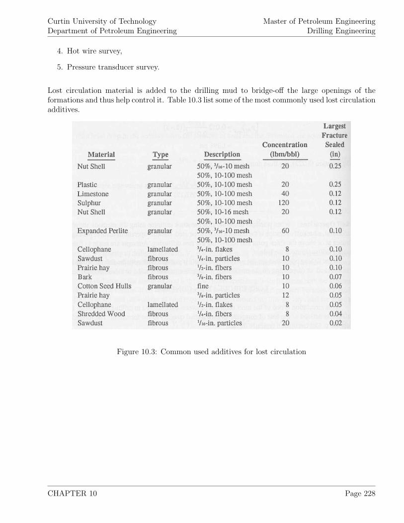
Curtin University of TechnologyDepartment of Petroleum Engineering
Master of Petroleum EngineeringDrilling Engineering
4. Hot wire survey,
5. Pressure transducer survey.
Lost circulation material is added to the drilling mud to bridge-off the large openings of theformations and thus help control it. Table 10.3 list some of the most commonly used lost circulationadditives.
Figure 10.3: Common used additives for lost circulation
CHAPTER 10 Page 228
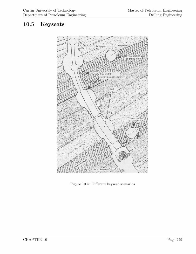
Curtin University of TechnologyDepartment of Petroleum Engineering
Master of Petroleum EngineeringDrilling Engineering
10.5 Keyseats
Figure 10.4: Different keyseat scenarios
CHAPTER 10 Page 229
Curtin University of TechnologyDepartment of Petroleum Engineering
Master of Petroleum EngineeringDrilling Engineering
10.6 Examples
1. In a 9,500 [ft] hole the drillstring is stuck at 8,000 [ft]. What is the volume of oil requiredto pump through the drillstring to free the pipe when the pore pressure is estimated to be 4,300[psi] at the stuck depth. Following further well data are available: ρm = 12 [ppg], ρo = 8 [ppg],Vdp = 0.0178 [bbl/ft], Van = 0.0544 [bbl/ft].
2. Determine the density, length and type of kick using the following information: Vk = 20 [bbl],Ldc = 900 [ft], ρm = 9.6 [ppg], d2 = 9.875 [in], d1c = 7.785 [in], dip = 4.2 [in], pc = 720 [psi],pdp = 520 [psi].
3. When drilling a 8-12
[in] hole, a kick is taken at 9,500 [ft]. After shutting in, the stabilizeddrillpipe pressure and the casing shut-in pressure are found to be 300 [psi] and 600 [psi] respectively.The recorded pit gain is 20 [bbl], pre-kick information contain: dh = 8.5 [in], ddc = 3.0 [in],ddp = 4.276 [in], Ldc = 600 [ft], Ddc = 8 [in], Ddp = 5 [in], ρm = 11 [ppg], (pp)str=60 = 2, 000 [psi],(pp)str=30 = 500 [psi]. Applying the wait-and-weight method, compute the:
(a) Bottom hole pressure,(b) Kill mud weight,(c) Standpipe pressure at start of circulation of
heavier mud,(d) Final circulation pressure,(e) Time required to replace the contents of the drillstring
with the kill mud,(f) Total time required to replace the contents of the
well with kill mud,(g) Total number of strokes required assuming that the
pump factor is 0.15 [bbl/stroke],(h) Maximum casing pressure when the kick reaches the surface,(i) Expected pit gain as the top of the kick reaches the surface.
CHAPTER 10 Page 230
Curtin University of TechnologyDepartment of Petroleum Engineering
Master of Petroleum EngineeringDrilling Engineering
Chapter 11
Kick Control and Blowout Prevention
A kick is defined as flow of formation fluids or gas into the wellbore, a blowout is the uncontrolledrelease of the fluid or gas, gained through the kick. A blowout can take place at the surface orinto another formation (underground blowout). Formation fluids that enter the wellbore can becrude oil or brine, gas entered can be any kind of naturally occurring gas. During a kick, drillingmud is displaced by the fluid or gas entering the borehole. To detect a kick, this is one of theeasiest warning signs, others are discussed below. Some causes of kicks may be:
1. Lost circulation, thus reduction of hydrostatic pressure,
2. Abnormally high pressured horizons drilled with to low mud weight,
3. Reduction of hydrostatic pressure while swabbing,
4. Failure to keep the borehole full of drilling fluid while tripping out.
A well control system permits:
1. Detecting a kick,
2. Closing the well at the surface,
3. Circulating the well under pressure to remove the formation fluids and increase the muddensity,
4. Moving the drillstring under pressure,
5. Diverting the flow away from the rig personnel and equipment.
To prevent a well from blowing out, it is essential to detect a kick as soon as possible. Especially atwildcat wells and wells drilled in areas of abnormal formation pressures, the various kick detectionparameters have to be observed continuously.
Kick Detection Parameters
CHAPTER 11 Page 231
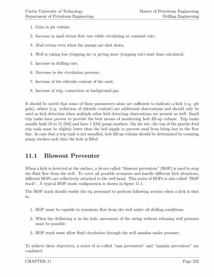
Curtin University of TechnologyDepartment of Petroleum Engineering
Master of Petroleum EngineeringDrilling Engineering
1. Gain in pit volume,
2. Increase in mud return flow rate while circulating at constant rate,
3. Mud return even when the pumps are shut down,
4. Well is taking less (tripping in) or giving more (tripping out) mud than calculated,
5. Increase in drilling rate,
6. Decrease in the circulation pressure,
7. Increase of the chloride content of the mud,
8. Increase of trip, connection or background gas.
It should be noted that some of these parameters alone are sufficient to indicate a kick (e.g. pitgain), others (e.g. reduction of chloride content) are additional observations and should only beused as kick detection when multiple other kick detecting observations are present as well. Smalltrip tanks have proven to provide the best means of monitoring hole fill-up volume. Trip tanksusually hold 10 to 15 [bbl] and have 1 [bbl] gauge markers. On the site, the top of the gravity-feedtrip tank must be slightly lower than the bell nipple to prevent mud from being lost to the flowline. In case that a trip tank is not installed, hole fill-up volume should be determined by countingpump strokes each time the hole is filled.
11.1 Blowout Preventer
When a kick is detected at the surface, a device called “blowout preventers” (BOP) is used to stopthe fluid flow from the well. To cover all possible scenarios and handle different kick situations,different BOPs are collectively attached to the well head. This series of BOPs is also called “BOPstack”. A typical BOP stack configuration is shown in figure 11.1.
The BOP stack should enable the rig personnel to perform following actions when a kick is shutin:
1. BOP must be capable to terminate flow from the well under all drilling conditions.
2. When the drillstring is in the hole, movement of the string without releasing well pressuremust be possible.
3. BOP stack must allow fluid circulation through the well annulus under pressure.
To achieve these objectives, a series of so called “ram preventers” and “annular preventers” arecombined.
CHAPTER 11 Page 232
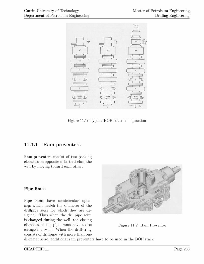
Curtin University of TechnologyDepartment of Petroleum Engineering
Master of Petroleum EngineeringDrilling Engineering
Figure 11.1: Typical BOP stack configuration
11.1.1 Ram preventers
Figure 11.2: Ram Preventer
Ram preventers consist of two packingelements on opposite sides that close thewell by moving toward each other.
Pipe Rams
Pipe rams have semicircular open-ings which match the diameter of thedrillpipe seize for which they are de-signed. Thus when the drillpipe seizeis changed during the well, the closingelements of the pipe rams have to bechanged as well. When the drillstringconsists of drillpipe with more than onediameter seize, additional ram preventers have to be used in the BOP stack.
CHAPTER 11 Page 233
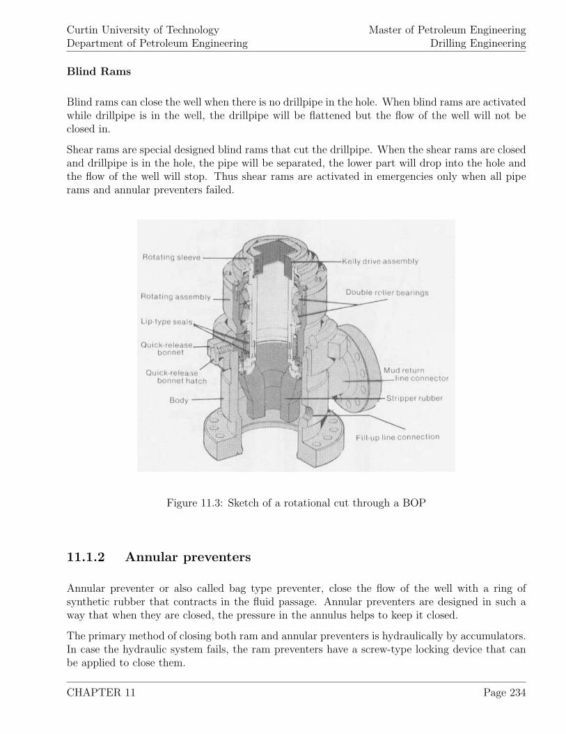
Curtin University of TechnologyDepartment of Petroleum Engineering
Master of Petroleum EngineeringDrilling Engineering
Blind Rams
Blind rams can close the well when there is no drillpipe in the hole. When blind rams are activatedwhile drillpipe is in the well, the drillpipe will be flattened but the flow of the well will not beclosed in.
Shear rams are special designed blind rams that cut the drillpipe. When the shear rams are closedand drillpipe is in the hole, the pipe will be separated, the lower part will drop into the hole andthe flow of the well will stop. Thus shear rams are activated in emergencies only when all piperams and annular preventers failed.
Figure 11.3: Sketch of a rotational cut through a BOP
11.1.2 Annular preventers
Annular preventer or also called bag type preventer, close the flow of the well with a ring ofsynthetic rubber that contracts in the fluid passage. Annular preventers are designed in such away that when they are closed, the pressure in the annulus helps to keep it closed.
The primary method of closing both ram and annular preventers is hydraulically by accumulators.In case the hydraulic system fails, the ram preventers have a screw-type locking device that canbe applied to close them.
CHAPTER 11 Page 234
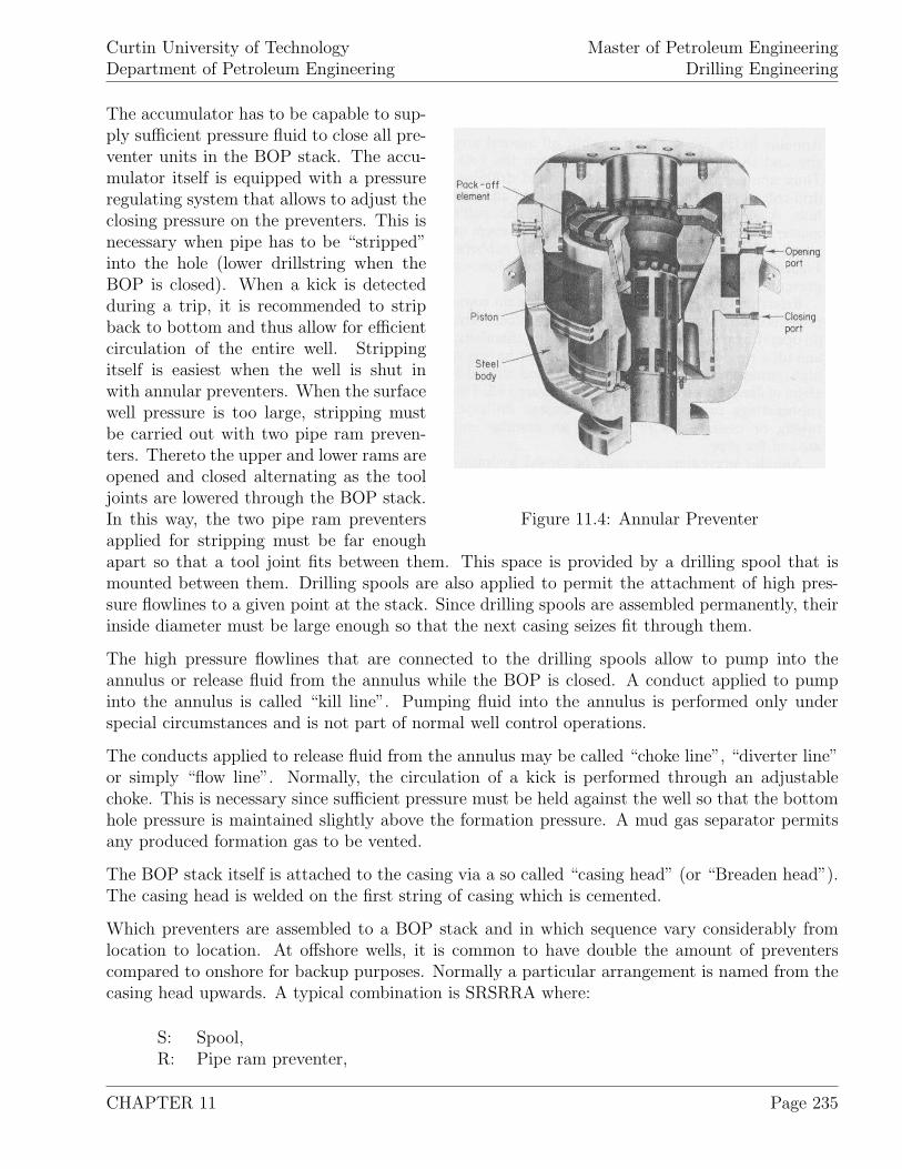
Curtin University of TechnologyDepartment of Petroleum Engineering
Master of Petroleum EngineeringDrilling Engineering
Figure 11.4: Annular Preventer
The accumulator has to be capable to sup-ply sufficient pressure fluid to close all pre-venter units in the BOP stack. The accu-mulator itself is equipped with a pressureregulating system that allows to adjust theclosing pressure on the preventers. This isnecessary when pipe has to be “stripped”into the hole (lower drillstring when theBOP is closed). When a kick is detectedduring a trip, it is recommended to stripback to bottom and thus allow for efficientcirculation of the entire well. Strippingitself is easiest when the well is shut inwith annular preventers. When the surfacewell pressure is too large, stripping mustbe carried out with two pipe ram preven-ters. Thereto the upper and lower rams areopened and closed alternating as the tooljoints are lowered through the BOP stack.In this way, the two pipe ram preventersapplied for stripping must be far enoughapart so that a tool joint fits between them. This space is provided by a drilling spool that ismounted between them. Drilling spools are also applied to permit the attachment of high pres-sure flowlines to a given point at the stack. Since drilling spools are assembled permanently, theirinside diameter must be large enough so that the next casing seizes fit through them.
The high pressure flowlines that are connected to the drilling spools allow to pump into theannulus or release fluid from the annulus while the BOP is closed. A conduct applied to pumpinto the annulus is called “kill line”. Pumping fluid into the annulus is performed only underspecial circumstances and is not part of normal well control operations.
The conducts applied to release fluid from the annulus may be called “choke line”, “diverter line”or simply “flow line”. Normally, the circulation of a kick is performed through an adjustablechoke. This is necessary since sufficient pressure must be held against the well so that the bottomhole pressure is maintained slightly above the formation pressure. A mud gas separator permitsany produced formation gas to be vented.
The BOP stack itself is attached to the casing via a so called “casing head” (or “Breaden head”).The casing head is welded on the first string of casing which is cemented.
Which preventers are assembled to a BOP stack and in which sequence vary considerably fromlocation to location. At offshore wells, it is common to have double the amount of preventerscompared to onshore for backup purposes. Normally a particular arrangement is named from thecasing head upwards. A typical combination is SRSRRA where:
S: Spool,R: Pipe ram preventer,
CHAPTER 11 Page 235
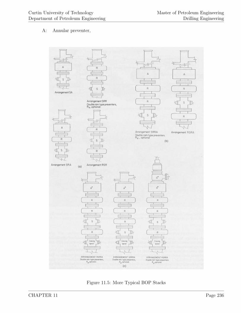
Curtin University of TechnologyDepartment of Petroleum Engineering
Master of Petroleum EngineeringDrilling Engineering
A: Annular preventer,
Figure 11.5: More Typical BOP Stacks
CHAPTER 11 Page 236
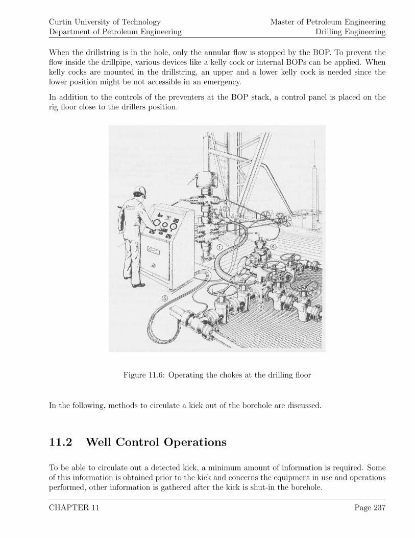
Curtin University of TechnologyDepartment of Petroleum Engineering
Master of Petroleum EngineeringDrilling Engineering
When the drillstring is in the hole, only the annular flow is stopped by the BOP. To prevent theflow inside the drillpipe, various devices like a kelly cock or internal BOPs can be applied. Whenkelly cocks are mounted in the drillstring, an upper and a lower kelly cock is needed since thelower position might be not accessible in an emergency.
In addition to the controls of the preventers at the BOP stack, a control panel is placed on therig floor close to the drillers position.
Figure 11.6: Operating the chokes at the drilling floor
In the following, methods to circulate a kick out of the borehole are discussed.
11.2 Well Control Operations
To be able to circulate out a detected kick, a minimum amount of information is required. Someof this information is obtained prior to the kick and concerns the equipment in use and operationsperformed, other information is gathered after the kick is shut-in the borehole.
CHAPTER 11 Page 237
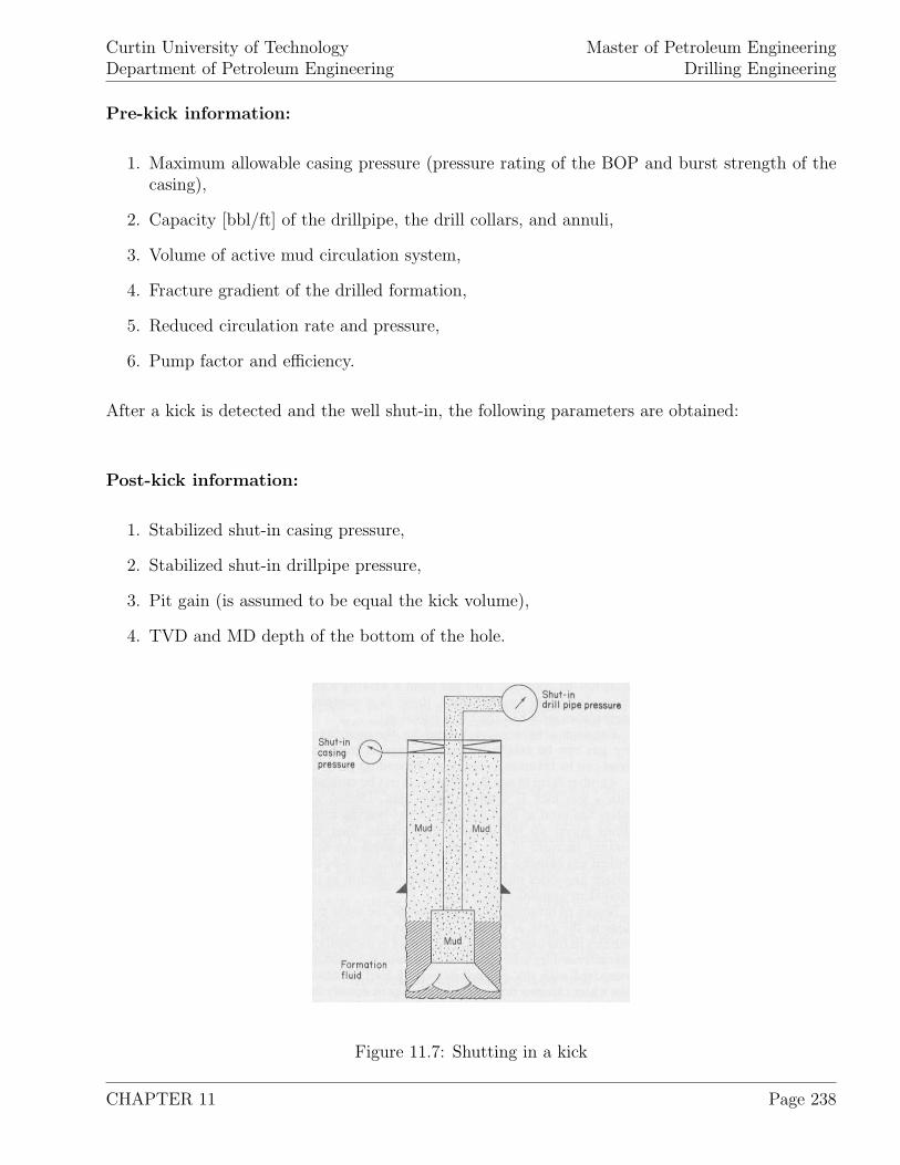
Curtin University of TechnologyDepartment of Petroleum Engineering
Master of Petroleum EngineeringDrilling Engineering
Pre-kick information:
1. Maximum allowable casing pressure (pressure rating of the BOP and burst strength of thecasing),
2. Capacity [bbl/ft] of the drillpipe, the drill collars, and annuli,
3. Volume of active mud circulation system,
4. Fracture gradient of the drilled formation,
5. Reduced circulation rate and pressure,
6. Pump factor and efficiency.
After a kick is detected and the well shut-in, the following parameters are obtained:
Post-kick information:
1. Stabilized shut-in casing pressure,
2. Stabilized shut-in drillpipe pressure,
3. Pit gain (is assumed to be equal the kick volume),
4. TVD and MD depth of the bottom of the hole.
Figure 11.7: Shutting in a kick
CHAPTER 11 Page 238
Curtin University of TechnologyDepartment of Petroleum Engineering
Master of Petroleum EngineeringDrilling Engineering
Having all the information at hand, following parameters are determined before attempting tocirculate out the kick:
1. Density (determines type) and length of kick,
2. Mud weight required to stop well from kicking,
3. Number of pump strokes to pump a volume from surface to bit and from bit to choke,
4. Volume of weighted mud to kill well,
5. Quantity of weighting material (e.g. barite) required to weight up the drilling fluid,
6. Accurate initial circulation drillpipe pressure,
7. Accurate final circulation drillpipe pressure,
8. Drillpipe pressure reduction schedule (for wait-and-weight method).
11.3 Length and Density of Kick
To determine the type of kick taken (oil, water, gas), the density of the gained fluid (kick density)has to be estimated. This is achieved by combining the observed drillpipe pdp and the casingpressure pc as well as the gain in pit volume. Equation 11.1 calculates the kick density [ppg]:
ρk = ρm − pc − pdp
0.052.Lk
(11.1)
To solve this equation, the kick length Lk [ft], which is estimated by the pit gain and the geomet-rical configuration of the drillstring and the diameter of the borehole, has to be computed first.For a pit gain Vk smaller or equal the annulus volume of the drill collars (Van)dc, the length of thekick is found by equation 11.2:
Lk = Vk. (Van)dc (11.2)
For a pit gain Vk larger than the annulus volume of the drill collars (Van)dc equation 11.3 has tobe used.
Lk = Ldc +
(Vk − Ldc
(Van)dc
). (Van)dp (11.3)
where:
CHAPTER 11 Page 239
Curtin University of TechnologyDepartment of Petroleum Engineering
Master of Petroleum EngineeringDrilling Engineering
(Van)cd [ft/bbl] ... annular capacity of the borehole at the drill collarsLdc [ft] ... total length of the drill collars(Van)dp [ft/bbl] ... annular capacity of the borehole at the drillpipeVk [bbl] ... kick volume, pit gainPc [psi] ... initial stabilized casing pressurePdp [psi] ... initial stabilized drillpipe pressure
Knowing the kick density, the so called kick gradient gradk [psi/ft] is often applied to identify thetype of kick. The kick gradient is computed as:
gradk = 0.052.ρk (11.4)
where:
ρk [ppg] ... kick density
Thus:
gradk < 0.3 ... gas kick0.3 < gradk < 0.4 ... oil and gas mixture
gradk > 0.4 ... water kickgradk > 8.33 ... salt water kick
11.4 Kick Tolerance and Kill Mud Weight
The kick tolerance determines the ability to control a kick at the current situation without frac-turing a formation and causing lost circulation.
By definition, the kick tolerance is the difference between the maximum pore pressure of anyformation penetrated and causing the kick, and the drilling mud weight at this depth. This ismathematically expressed as:
Tk = (ρe − ρm) (11.5)
To establish safe drilling condition, it should be ensured that the kick tolerance is never below 1[ppg]. The kill mud weight is defined as the mud weight required to stop a well from kicking andcan be computed by:
CHAPTER 11 Page 240
Curtin University of TechnologyDepartment of Petroleum Engineering
Master of Petroleum EngineeringDrilling Engineering
ρkm = ρm +pdp
0.052.D(11.6)
The equivalent mud density at the casing seat is found as:
ρe =pc
0.052.Dc
+ ρm (11.7)
where:
Dc [ft] ... casing setting depth
11.5 Pump Pressure Schedules for Well Control Opera-
tions
When killing a well, the bottom hole pressure of the well must be maintained equal to or higherthan the formation pressure which caused the kick. When this is not established, the well wouldbe constantly kicking, thus constantly gaining formation fluid or gas.
To maintain this required bottom hole pressure, the circulation pressure to remove the kick hasto be calculated as planned pump rate for kick removal. Normally, the pump rate to circulateout a kick is half the drilling pump rate. It is common practice to calculate the required circu-lation pressure since the required bottom hole pressure is not directly measurable. The requiredcirculation pressure can be found as:
pdpff = pdp + ∆pp − ∆pdpf = pdpf − ∆pdpf (11.8)
where:
∆pdpf = (ρkm − ρm) .
(0.052.D − ∆pp
ρm
)(11.9)
This enables the calculation of the total number of pump strokes required to pump the kill mudto the bit:
fstr =Ldp.Vdp + Ldc.Vdc
Fp
(11.10)
where:
CHAPTER 11 Page 241
Curtin University of TechnologyDepartment of Petroleum Engineering
Master of Petroleum EngineeringDrilling Engineering
pdpff [psi] ... final circulation drillpipe pressure∆pdpf [psi] ... change in total drillpipe pressure required
to maintain the bottom hole pressure constant∆pp [psi] ... routinely measured circulation pump pressureFp [bbl/stroke] ... pump factorLdp [ft] ... length of drillpipeLdc [ft] ... length of drill collarsVdp [bbl/ft] ... capacity of drillpipeVdc [bbl/ft] ... capacity of drill collar
The number of strokes pumped and the circulation drillpipe pressure are linearly related. Thiscan be seen with equation 11.11:
dpn = pdpf −(
pdpf − pdpff
fstr
).Str (11.11)
where:
Str [# strokes] ... intermediate pump strokes
11.6 Kick Removal – Two Methods
In general, two methods to circulate a kick out are applied most often:
1. Driller’s method,
2. Wait-and-weight method.
At the wait-and-weight method, the well is closed-in once a kick is detected and the post-kickinformation is obtained. Next, the kill mud weight is determined, the weighted mud is preparedand then circulated in to kill the well. During this operation, the drillpipe pressure is checkedaccording to the pressure schedule which has to be prepared before the circulation starts.
When the driller’s method is applied to kill the well, the whole process is divided into two steps.First, the annulus fluid containing the kick is displaced with the help of an adjustable choke.Normally, circulation is continued so that all kick fluids are removed. Then, as a second step, theweighted mud is pumped through the drillstring and the annulus by a complete circulation.
The driller’s methods offers following advantages compared to the weight-and-weight method:
1. Circulation starts immediately,
CHAPTER 11 Page 242
Curtin University of TechnologyDepartment of Petroleum Engineering
Master of Petroleum EngineeringDrilling Engineering
2. Sufficient time is given to weighting up the mud.
The disadvantages of the driller’s method compared to the wait-and-weight method are:
1. Maximum surface pressure and pressure at the casing shoe are higher,
2. Surface equipment is subjected to higher pressures for a longer time.
11.6.1 Wait-and-weight method
pbh = pdp + 0.052.ρm.D (11.12)
G =Vk.pbh
pmax
(11.13)
pmax =
√b2 + 4.c + b
2(11.14)
b =pdp.Vdp. (Van)dp
D+ 0.052.ρkm.D1 (11.15)
c = 0.052.ρkm.Vk. (Van)dp .pbh (11.16)
where:
pbh [psi] ... bottom hole pressureG [bbl] ... pit volume increase when top of kick reaches the depth of interestpmax [psi] ... maximum casing pressureVdp [bbl] ... inside drillpipe capacity(Van)dp [ft/bbl] ... annular capacity opposite the drillpipeD1 [ft] ... depth to the point where kick severity calculation is requiredρm [ppg] ... kill mud weightD [ft] ... total depth of the well
CHAPTER 11 Page 243
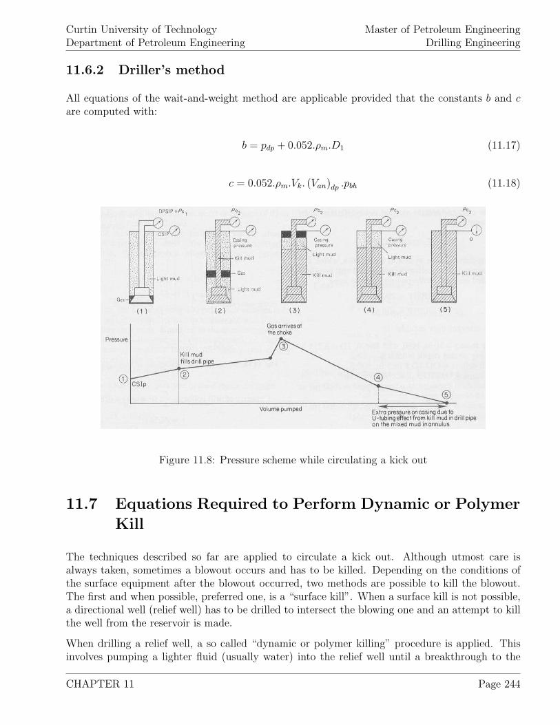
Curtin University of TechnologyDepartment of Petroleum Engineering
Master of Petroleum EngineeringDrilling Engineering
11.6.2 Driller’s method
All equations of the wait-and-weight method are applicable provided that the constants b and care computed with:
b = pdp + 0.052.ρm.D1 (11.17)
c = 0.052.ρm.Vk. (Van)dp .pbh (11.18)
Figure 11.8: Pressure scheme while circulating a kick out
11.7 Equations Required to Perform Dynamic or Polymer
Kill
The techniques described so far are applied to circulate a kick out. Although utmost care isalways taken, sometimes a blowout occurs and has to be killed. Depending on the conditions ofthe surface equipment after the blowout occurred, two methods are possible to kill the blowout.The first and when possible, preferred one, is a “surface kill”. When a surface kill is not possible,a directional well (relief well) has to be drilled to intersect the blowing one and an attempt to killthe well from the reservoir is made.
When drilling a relief well, a so called “dynamic or polymer killing” procedure is applied. Thisinvolves pumping a lighter fluid (usually water) into the relief well until a breakthrough to the
CHAPTER 11 Page 244
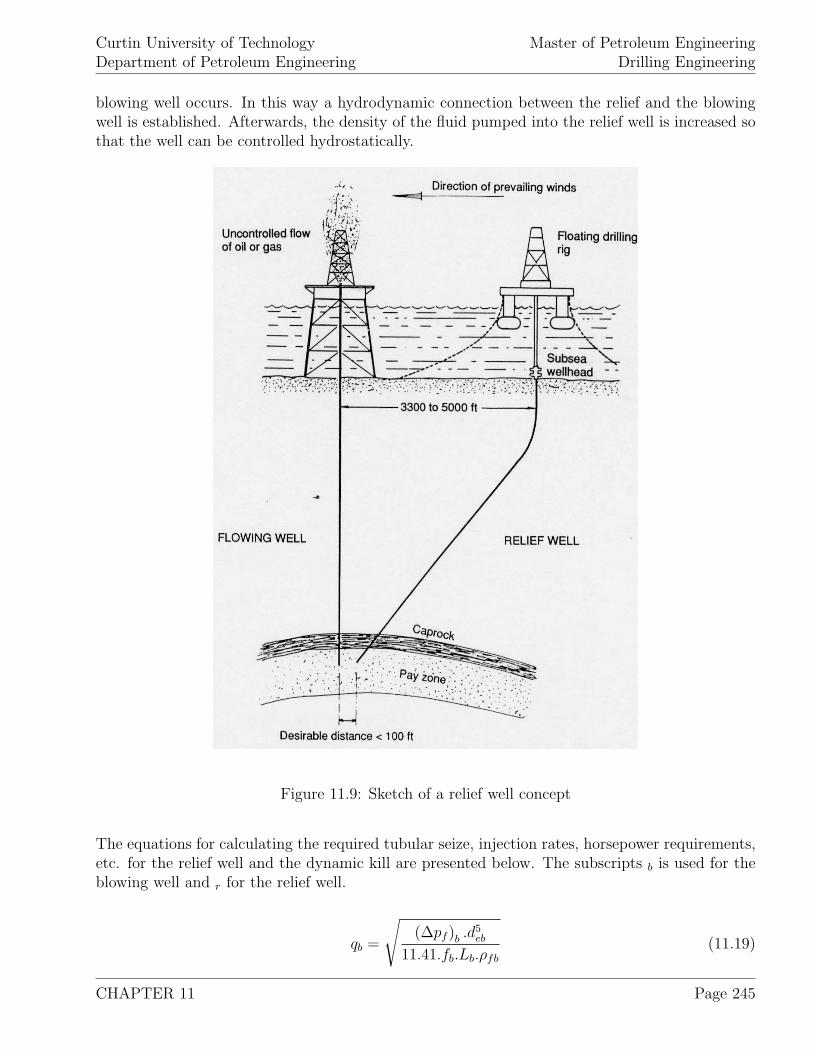
Curtin University of TechnologyDepartment of Petroleum Engineering
Master of Petroleum EngineeringDrilling Engineering
blowing well occurs. In this way a hydrodynamic connection between the relief and the blowingwell is established. Afterwards, the density of the fluid pumped into the relief well is increased sothat the well can be controlled hydrostatically.
Figure 11.9: Sketch of a relief well concept
The equations for calculating the required tubular seize, injection rates, horsepower requirements,etc. for the relief well and the dynamic kill are presented below. The subscripts b is used for theblowing well and r for the relief well.
qb =
√(∆pf )b .d5
eb
11.41.fb.Lb.ρfb
(11.19)
CHAPTER 11 Page 245
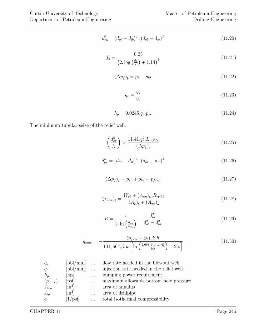
Curtin University of TechnologyDepartment of Petroleum Engineering
Master of Petroleum EngineeringDrilling Engineering
d5eb = (dob − dib)
3 . (dob − dib)2 (11.20)
fb =0.25(
2. log(
dh
ε
)+ 1.14
)2 (11.21)
(∆pf )b = pb − phb (11.22)
qr =qb
ηe
(11.23)
hp = 0.0245.qr.psr (11.24)
The minimum tubular seize of the relief well:
(d5
er
fr
)>
11.41.q2r .Lr.ρfr
(∆pf )r
(11.25)
d5er = (dor − dir)
3 . (dor − dir)2 (11.26)
(∆pf )r = psr + phr − pfrac (11.27)
(pmax)b =Wsb + (Aan)b .R.phb
(Ap)b + (Aan)b
(11.28)
R =1
2. ln(
dob
dib
) − d2ib
d2ob − d2
ib
(11.29)
qmax = − (pfrac − pb) .k.h
101, 664.β.µ.[ln
(1,688.φ.µ.ct.r2
w
k.t
)− 2.s
] (11.30)
qb [bbl/min] ... flow rate needed in the blowout wellqr [bbl/min] ... injection rate needed in the relief wellhp [hp] ... pumping power requirement(pmax)b [psi] ... maximum allowable bottom hole pressureAan [in2] ... area of annulusAp [in2] ... area of drillpipect [1/psi] ... total isothermal compressibility
CHAPTER 11 Page 246
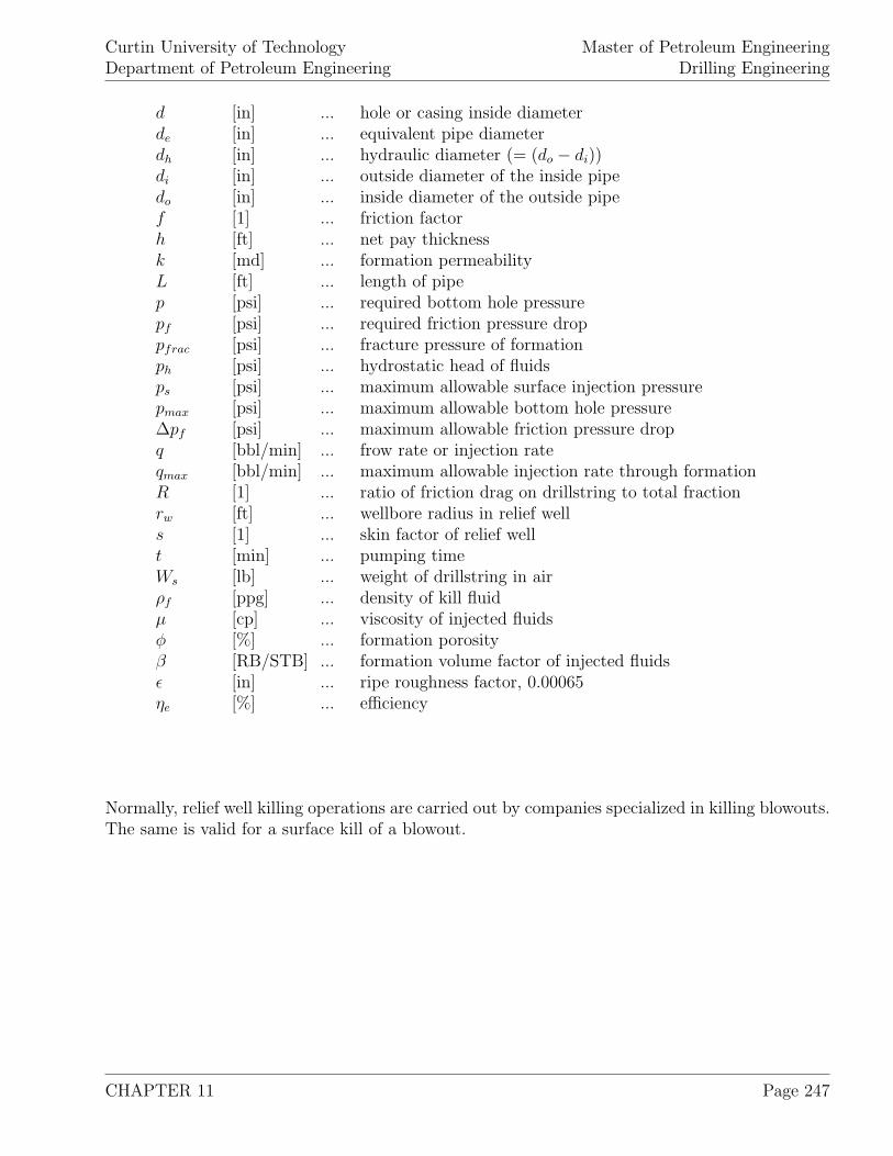
Curtin University of TechnologyDepartment of Petroleum Engineering
Master of Petroleum EngineeringDrilling Engineering
d [in] ... hole or casing inside diameterde [in] ... equivalent pipe diameterdh [in] ... hydraulic diameter (= (do − di))di [in] ... outside diameter of the inside pipedo [in] ... inside diameter of the outside pipef [1] ... friction factorh [ft] ... net pay thicknessk [md] ... formation permeabilityL [ft] ... length of pipep [psi] ... required bottom hole pressurepf [psi] ... required friction pressure droppfrac [psi] ... fracture pressure of formationph [psi] ... hydrostatic head of fluidsps [psi] ... maximum allowable surface injection pressurepmax [psi] ... maximum allowable bottom hole pressure∆pf [psi] ... maximum allowable friction pressure dropq [bbl/min] ... frow rate or injection rateqmax [bbl/min] ... maximum allowable injection rate through formationR [1] ... ratio of friction drag on drillstring to total fractionrw [ft] ... wellbore radius in relief wells [1] ... skin factor of relief wellt [min] ... pumping timeWs [lb] ... weight of drillstring in airρf [ppg] ... density of kill fluidµ [cp] ... viscosity of injected fluidsφ [%] ... formation porosityβ [RB/STB] ... formation volume factor of injected fluidsε [in] ... ripe roughness factor, 0.00065ηe [%] ... efficiency
Normally, relief well killing operations are carried out by companies specialized in killing blowouts.The same is valid for a surface kill of a blowout.
CHAPTER 11 Page 247

Curtin University of TechnologyDepartment of Petroleum Engineering
Master of Petroleum EngineeringDrilling Engineering
11.8 Examples
CHAPTER 11 Page 248
Curtin University of TechnologyDepartment of Petroleum Engineering
Master of Petroleum EngineeringDrilling Engineering
Chapter 12
Cementing
Cementing an oil or gas well comprises the displacement of cement slurry down the drillstring,tubing or casing to a predefined section of the annulus of the well. The cement slurry itselftypically contains water, portland cement and various additives. The actual composition variesfrom application to application.
Different cement slurry placement techniques are:
1. primary cementing,
2. liner cementing,
3. squeeze cementing,
4. plug back cementing.
12.1 Functions of Cement
The functions of the different cement jobs differ according to the various objectives. The list belowgives of some main objectives for the different cement jobs.
Primary Cement
1. Isolate a hydrocarbon bearing formation from other formations,
2. Protect and secure the casing in the well,
3. Prevent caving of the hole,
4. Provide a firm seal and anchor for the wellhead equipment,
5. Protect casing from corrosion by sulfate rich formation waters.
CHAPTER 12 Page 249
Curtin University of TechnologyDepartment of Petroleum Engineering
Master of Petroleum EngineeringDrilling Engineering
Liner Cement
1. Case off open hole below a long intermediate casing,
2. Case off open hole resulting from casing stuck at the bottom,
3. Case off previous open-hole completion in order to control water, gas or sand,
4. Case off zones of lost circulation or high pressure zones encountered during drilling,
Squeeze Cement
1. Reduce water-oil, water-gas, or gas-oil ratios,
2. Shut off a zone that is been depleted, is not economical to produce or whose production willbe delayed until the more promising zones in the same borehole are depleted,
3. Isolate a zone before perforating for production or stimulation,
4. Supplement a faulty primary cement job,
5. Repair casing or joint leaks, spit or parted casing,
6. Stop lost circulation in an open hole while drilling.
Plug Back Cement
1. Shut off bottom hole water production,
2. Abandon permanently deeper zones,
3. Completing a zone uphole,
4. Place a cement bridge plug,
5. Set plug to provide a seat for directional tools like whipstock,
6. Set plug in unintentionally deviated well when vertical trajectory is intended. After settingthe plug the vertical hole is continued.
7. Set plug through keyseat portion of the well and redrill it.
CHAPTER 12 Page 250
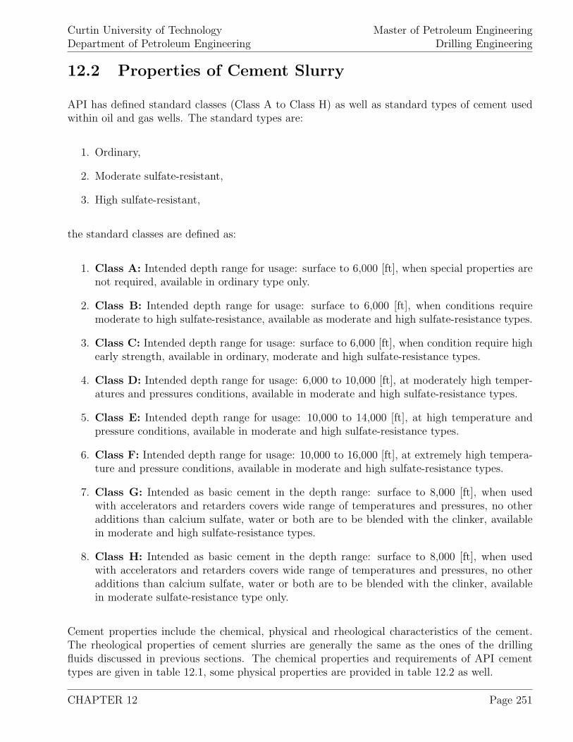
Curtin University of TechnologyDepartment of Petroleum Engineering
Master of Petroleum EngineeringDrilling Engineering
12.2 Properties of Cement Slurry
API has defined standard classes (Class A to Class H) as well as standard types of cement usedwithin oil and gas wells. The standard types are:
1. Ordinary,
2. Moderate sulfate-resistant,
3. High sulfate-resistant,
the standard classes are defined as:
1. Class A: Intended depth range for usage: surface to 6,000 [ft], when special properties arenot required, available in ordinary type only.
2. Class B: Intended depth range for usage: surface to 6,000 [ft], when conditions requiremoderate to high sulfate-resistance, available as moderate and high sulfate-resistance types.
3. Class C: Intended depth range for usage: surface to 6,000 [ft], when condition require highearly strength, available in ordinary, moderate and high sulfate-resistance types.
4. Class D: Intended depth range for usage: 6,000 to 10,000 [ft], at moderately high temper-atures and pressures conditions, available in moderate and high sulfate-resistance types.
5. Class E: Intended depth range for usage: 10,000 to 14,000 [ft], at high temperature andpressure conditions, available in moderate and high sulfate-resistance types.
6. Class F: Intended depth range for usage: 10,000 to 16,000 [ft], at extremely high tempera-ture and pressure conditions, available in moderate and high sulfate-resistance types.
7. Class G: Intended as basic cement in the depth range: surface to 8,000 [ft], when usedwith accelerators and retarders covers wide range of temperatures and pressures, no otheradditions than calcium sulfate, water or both are to be blended with the clinker, availablein moderate and high sulfate-resistance types.
8. Class H: Intended as basic cement in the depth range: surface to 8,000 [ft], when usedwith accelerators and retarders covers wide range of temperatures and pressures, no otheradditions than calcium sulfate, water or both are to be blended with the clinker, availablein moderate sulfate-resistance type only.
Cement properties include the chemical, physical and rheological characteristics of the cement.The rheological properties of cement slurries are generally the same as the ones of the drillingfluids discussed in previous sections. The chemical properties and requirements of API cementtypes are given in table 12.1, some physical properties are provided in table 12.2 as well.
CHAPTER 12 Page 251
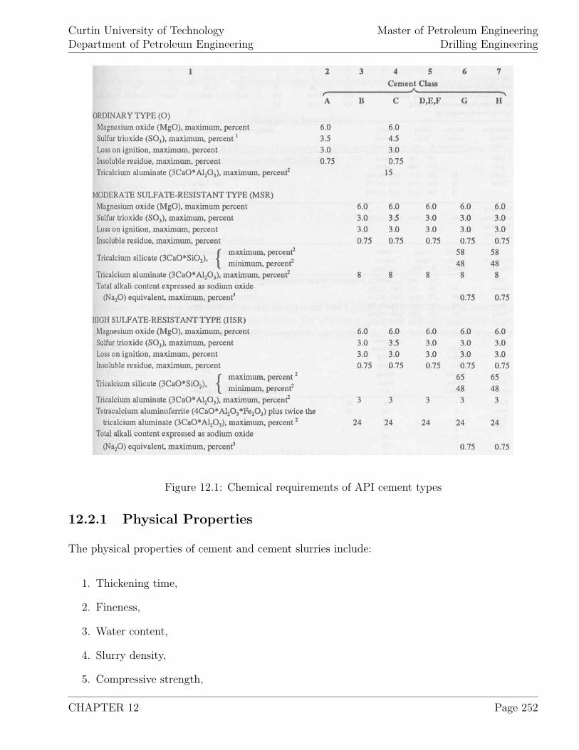
Curtin University of TechnologyDepartment of Petroleum Engineering
Master of Petroleum EngineeringDrilling Engineering
Figure 12.1: Chemical requirements of API cement types
12.2.1 Physical Properties
The physical properties of cement and cement slurries include:
1. Thickening time,
2. Fineness,
3. Water content,
4. Slurry density,
5. Compressive strength,
CHAPTER 12 Page 252
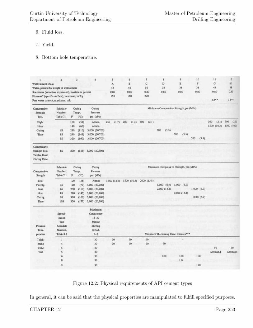
Curtin University of TechnologyDepartment of Petroleum Engineering
Master of Petroleum EngineeringDrilling Engineering
6. Fluid loss,
7. Yield,
8. Bottom hole temperature.
Figure 12.2: Physical requirements of API cement types
In general, it can be said that the physical properties are manipulated to fulfill specified purposes.
CHAPTER 12 Page 253
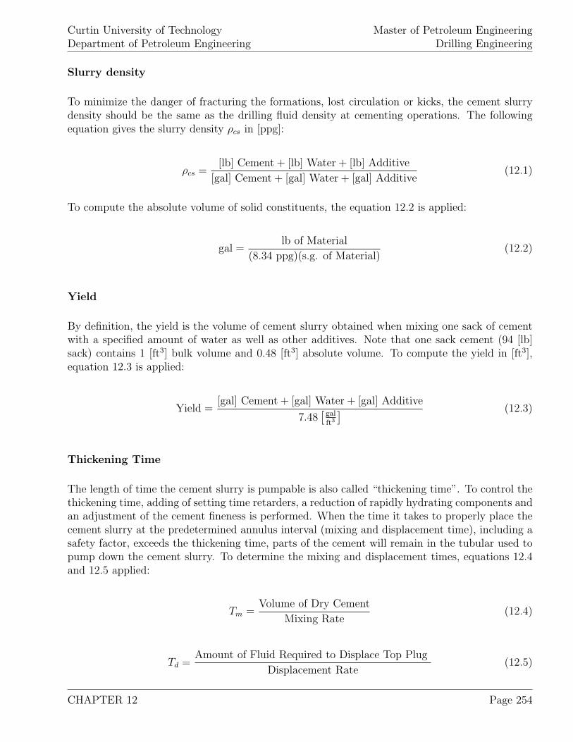
Curtin University of TechnologyDepartment of Petroleum Engineering
Master of Petroleum EngineeringDrilling Engineering
Slurry density
To minimize the danger of fracturing the formations, lost circulation or kicks, the cement slurrydensity should be the same as the drilling fluid density at cementing operations. The followingequation gives the slurry density ρcs in [ppg]:
ρcs =[lb] Cement + [lb] Water + [lb] Additive
[gal] Cement + [gal] Water + [gal] Additive(12.1)
To compute the absolute volume of solid constituents, the equation 12.2 is applied:
gal =lb of Material
(8.34 ppg)(s.g. of Material)(12.2)
Yield
By definition, the yield is the volume of cement slurry obtained when mixing one sack of cementwith a specified amount of water as well as other additives. Note that one sack cement (94 [lb]sack) contains 1 [ft3] bulk volume and 0.48 [ft3] absolute volume. To compute the yield in [ft3],equation 12.3 is applied:
Yield =[gal] Cement + [gal] Water + [gal] Additive
7.48[
galft3
] (12.3)
Thickening Time
The length of time the cement slurry is pumpable is also called “thickening time”. To control thethickening time, adding of setting time retarders, a reduction of rapidly hydrating components andan adjustment of the cement fineness is performed. When the time it takes to properly place thecement slurry at the predetermined annulus interval (mixing and displacement time), including asafety factor, exceeds the thickening time, parts of the cement will remain in the tubular used topump down the cement slurry. To determine the mixing and displacement times, equations 12.4and 12.5 applied:
Tm =Volume of Dry Cement
Mixing Rate(12.4)
Td =Amount of Fluid Required to Displace Top Plug
Displacement Rate(12.5)
CHAPTER 12 Page 254
Curtin University of TechnologyDepartment of Petroleum Engineering
Master of Petroleum EngineeringDrilling Engineering
Compressive Strength
To hold the casing in place, enable support capability of the surface wellhead equipment and with-stand the differential pressures across the cement-formation interface, the compressive strength ofthe set and hardened cement has to be high enough. As general practice, 500 [psi] of compres-sive strength has to be developed by the hardening cement before any other downhole operationcommences. The time it takes the cement to reach this minimum compressive strength is oftenreferenced as “wait on cement” (WOC). During this time, other routine surface service operationsare usually carried out. The support capability of the cement is given by:
F = 0.969.Sc.do.H (12.6)
where:
F [lbf] ... support capabilitySc [psi] ... compressive strength of cementdo [in] ... outside diameter of casingH [ft] ... hight of cement column
12.3 Cement Additives
Main component of all cement slurries for oil and gas well cementing is “Portland cement”. It isproduced according to API specifications by taking raw material like limestone, clay or shale, andiron ore. After mixing and grinding, they are fed into a kiln where they are melt into a substancecalled “cement clinker”. This clinker is then ground into a powdery mixture and combined withsmall amounts of gypsum or other components.
To better fit the individual well requirements, the properties of the cement slurry and hardenedcement have to be adjusted. Therefore, certain cement additives are mixed into the slurry. Theadditives can be grouped according to their functionality into:
1. Extenders,
2. Accelerators,
3. Retarders,
4. Weighting material,
5. Fluid loss or filtration control material,
6. Dispersants or thinners.
CHAPTER 12 Page 255
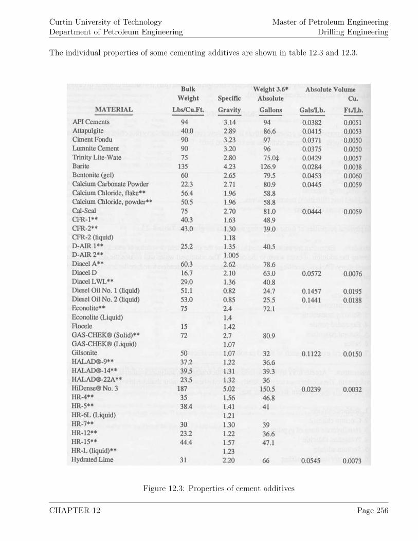
Curtin University of TechnologyDepartment of Petroleum Engineering
Master of Petroleum EngineeringDrilling Engineering
The individual properties of some cementing additives are shown in table 12.3 and 12.3.
Figure 12.3: Properties of cement additives
CHAPTER 12 Page 256
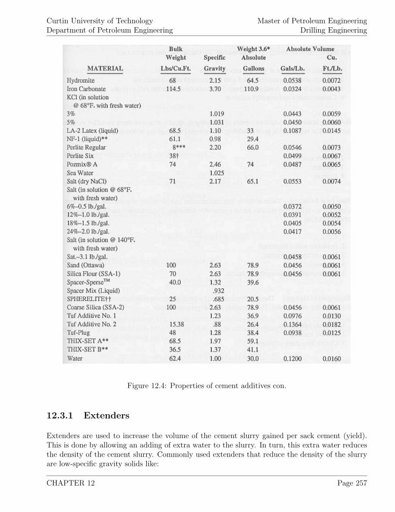
Curtin University of TechnologyDepartment of Petroleum Engineering
Master of Petroleum EngineeringDrilling Engineering
Figure 12.4: Properties of cement additives con.
12.3.1 Extenders
Extenders are used to increase the volume of the cement slurry gained per sack cement (yield).This is done by allowing an adding of extra water to the slurry. In turn, this extra water reducesthe density of the cement slurry. Commonly used extenders that reduce the density of the slurryare low-specific gravity solids like:
CHAPTER 12 Page 257
Curtin University of TechnologyDepartment of Petroleum Engineering
Master of Petroleum EngineeringDrilling Engineering
1. Bentonite,
2. Diatomaceous earth,
3. Solid hydrocarbons,
4. Expanded perlite,
5. Natural pozzolans,
6. Silica,
7. Chemical extenders (liquid or solid silicate).
12.3.2 Accelerators
To reduce the thickening time as well as increase the rate of early strength and thus reducethe WOC time, accelerators are added to the cement slurries. When cementing shallow, lowtemperature section of wells, accelerators are often essential. Commonly applied accelerators are:
1. Sodium chloride,
2. Calcium chloride,
3. Hemihydrate form of gypsum ,
4. Potassium chloride,
5. Sodium silicate,
6. Sea water for mixing.
12.3.3 Retarders
In contrary to the accelerators, retarders are added to cement slurries to prolong the thickeningtime and decrease the rate of early strength development. Deflocculants discussed as drilling fluidsadditives tend to delay the setting of cement, thus they are applied as retarders.
1. Calcium lignosulfate at very low concentrations,
2. Calcium-sodium lignosulfate used with high concentration of bentonite,
3. Sodium tetraborate decahydrate (borax) used as a catalyst for the deflocculants,
4. Carboxymethyl hydroxyethyl cellulose.
CHAPTER 12 Page 258
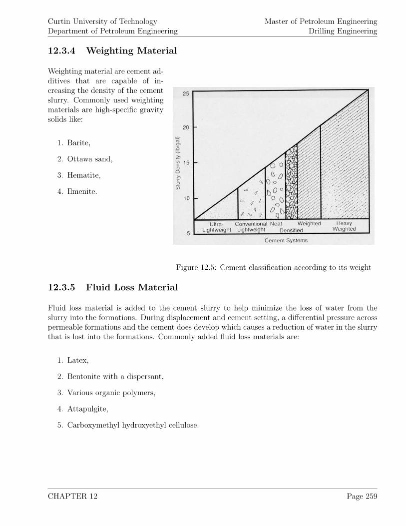
Curtin University of TechnologyDepartment of Petroleum Engineering
Master of Petroleum EngineeringDrilling Engineering
12.3.4 Weighting Material
Figure 12.5: Cement classification according to its weight
Weighting material are cement ad-ditives that are capable of in-creasing the density of the cementslurry. Commonly used weightingmaterials are high-specific gravitysolids like:
1. Barite,
2. Ottawa sand,
3. Hematite,
4. Ilmenite.
12.3.5 Fluid Loss Material
Fluid loss material is added to the cement slurry to help minimize the loss of water from theslurry into the formations. During displacement and cement setting, a differential pressure acrosspermeable formations and the cement does develop which causes a reduction of water in the slurrythat is lost into the formations. Commonly added fluid loss materials are:
1. Latex,
2. Bentonite with a dispersant,
3. Various organic polymers,
4. Attapulgite,
5. Carboxymethyl hydroxyethyl cellulose.
CHAPTER 12 Page 259
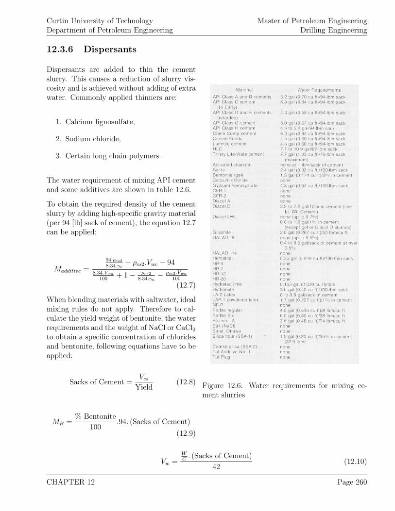
Curtin University of TechnologyDepartment of Petroleum Engineering
Master of Petroleum EngineeringDrilling Engineering
12.3.6 Dispersants
Figure 12.6: Water requirements for mixing ce-ment slurries
Dispersants are added to thin the cementslurry. This causes a reduction of slurry vis-cosity and is achieved without adding of extrawater. Commonly applied thinners are:
1. Calcium lignosulfate,
2. Sodium chloride,
3. Certain long chain polymers.
The water requirement of mixing API cementand some additives are shown in table 12.6.
To obtain the required density of the cementslurry by adding high-specific gravity material(per 94 [lb] sack of cement), the equation 12.7can be applied:
Madditive =
94.ρcs2
8.34.γc+ ρcs2.Vwc − 94
8.34.Vwa
100+ 1 − ρcs2
8.34.γa− ρcs2.Vwa
100
(12.7)
When blending materials with saltwater, idealmixing rules do not apply. Therefore to cal-culate the yield weight of bentonite, the waterrequirements and the weight of NaCl or CaCl2to obtain a specific concentration of chloridesand bentonite, following equations have to beapplied:
Sacks of Cement =Vcs
Yield(12.8)
MB =% Bentonite
100.94. (Sacks of Cement)
(12.9)
Vw =WC
. (Sacks of Cement)
42(12.10)
CHAPTER 12 Page 260
Curtin University of TechnologyDepartment of Petroleum Engineering
Master of Petroleum EngineeringDrilling Engineering
MChlorides =% Chlorides
100.94. (Sacks of Cement) (12.11)
% Chloride/Wt. of Water =94. (% Chloride)
8.34.WC
+ 94. (% Chloride/100)(12.12)
Yield = 0.47975 + 0.56846.
(% Bentonite
100
)+
(94. (% Chloride/100) + 8.34.W
C
62.4.γChlorides
)(12.13)
where:
Vwa [gal/sack] ... water requirement for additiveVwc [gal/sack] ... water requirement for cementγa [s.g.] ... specific gravity of additiveγc [s.g.] ... specific gravity of cementρcs2 [ppg] ... density of weighted slurryMadditive [lb/sack] ... weight of additive required to raise the density to ρcs2
Vcs [ft3] ... slurry volumeWC
[gal/sack] ... water/cement ratioγchlorides [s.g.] ... specific gravity of salt water as per percent chloridesMB [lb] ... weight of bentonite to be addedMchlorides [lb] ... weight of chlorides to be added
yield [ft3/sack]
% Cloride is the % NaCl or % CaCl2 by weight of cement
% Bentonite ie % bentonite by weight of cement
Specific gravities with respect to various concentrations of NaCl and CaCl2 are shown in tables12.7 and 12.8.
CHAPTER 12 Page 261
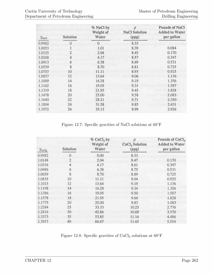
Curtin University of TechnologyDepartment of Petroleum Engineering
Master of Petroleum EngineeringDrilling Engineering
Figure 12.7: Specific gravities of NaCl solutions at 68◦F
Figure 12.8: Specific gravities of CaCl2 solutions at 68◦F
CHAPTER 12 Page 262
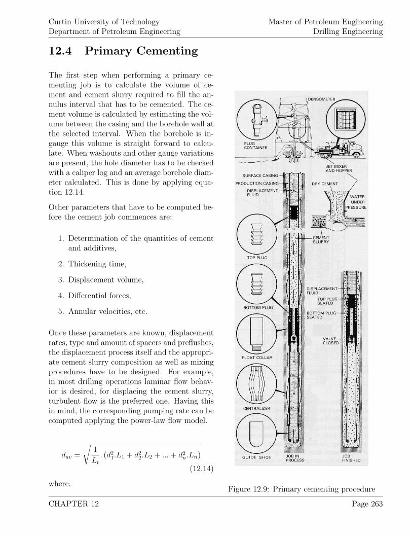
Curtin University of TechnologyDepartment of Petroleum Engineering
Master of Petroleum EngineeringDrilling Engineering
12.4 Primary Cementing
Figure 12.9: Primary cementing procedure
The first step when performing a primary ce-menting job is to calculate the volume of ce-ment and cement slurry required to fill the an-nulus interval that has to be cemented. The ce-ment volume is calculated by estimating the vol-ume between the casing and the borehole wall atthe selected interval. When the borehole is in-gauge this volume is straight forward to calcu-late. When washouts and other gauge variationsare present, the hole diameter has to be checkedwith a caliper log and an average borehole diam-eter calculated. This is done by applying equa-tion 12.14.
Other parameters that have to be computed be-fore the cement job commences are:
1. Determination of the quantities of cementand additives,
2. Thickening time,
3. Displacement volume,
4. Differential forces,
5. Annular velocities, etc.
Once these parameters are known, displacementrates, type and amount of spacers and preflushes,the displacement process itself and the appropri-ate cement slurry composition as well as mixingprocedures have to be designed. For example,in most drilling operations laminar flow behav-ior is desired, for displacing the cement slurry,turbulent flow is the preferred one. Having thisin mind, the corresponding pumping rate can becomputed applying the power-law flow model.
dav =
√1
Lt
. (d21.L1 + d2
2.L2 + ... + d2n.Ln)
(12.14)
where:
CHAPTER 12 Page 263
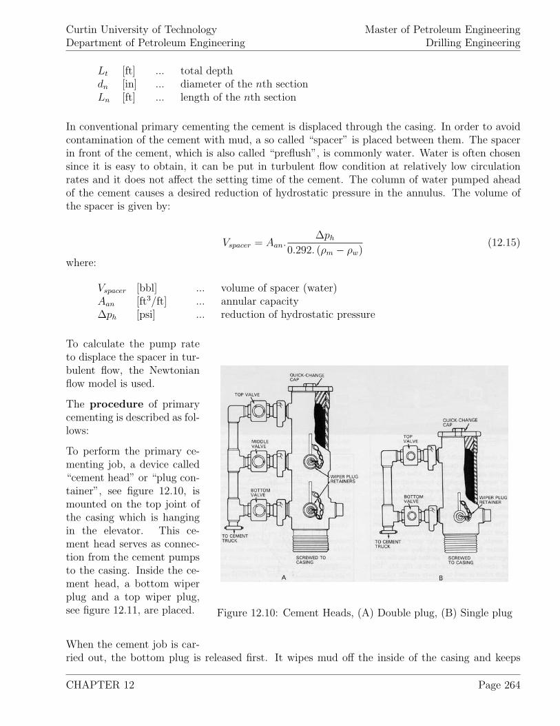
Curtin University of TechnologyDepartment of Petroleum Engineering
Master of Petroleum EngineeringDrilling Engineering
Lt [ft] ... total depthdn [in] ... diameter of the nth sectionLn [ft] ... length of the nth section
In conventional primary cementing the cement is displaced through the casing. In order to avoidcontamination of the cement with mud, a so called “spacer” is placed between them. The spacerin front of the cement, which is also called “preflush”, is commonly water. Water is often chosensince it is easy to obtain, it can be put in turbulent flow condition at relatively low circulationrates and it does not affect the setting time of the cement. The column of water pumped aheadof the cement causes a desired reduction of hydrostatic pressure in the annulus. The volume ofthe spacer is given by:
Vspacer = Aan.∆ph
0.292. (ρm − ρw)(12.15)
where:
Vspacer [bbl] ... volume of spacer (water)Aan [ft3/ft] ... annular capacity∆ph [psi] ... reduction of hydrostatic pressure
Figure 12.10: Cement Heads, (A) Double plug, (B) Single plug
To calculate the pump rateto displace the spacer in tur-bulent flow, the Newtonianflow model is used.
The procedure of primarycementing is described as fol-lows:
To perform the primary ce-menting job, a device called“cement head” or “plug con-tainer”, see figure 12.10, ismounted on the top joint ofthe casing which is hangingin the elevator. This ce-ment head serves as connec-tion from the cement pumpsto the casing. Inside the ce-ment head, a bottom wiperplug and a top wiper plug,see figure 12.11, are placed.
When the cement job is car-ried out, the bottom plug is released first. It wipes mud off the inside of the casing and keeps
CHAPTER 12 Page 264
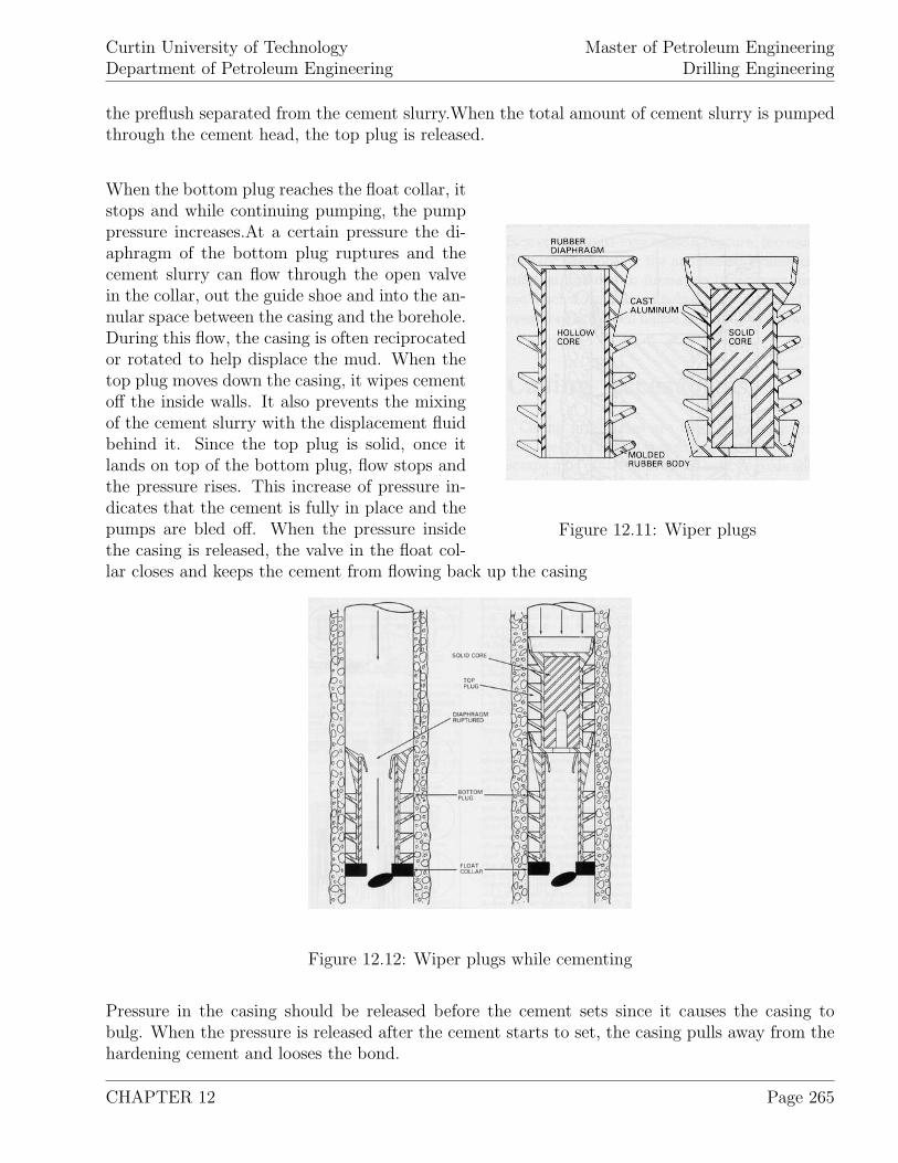
Curtin University of TechnologyDepartment of Petroleum Engineering
Master of Petroleum EngineeringDrilling Engineering
the preflush separated from the cement slurry.When the total amount of cement slurry is pumpedthrough the cement head, the top plug is released.
Figure 12.11: Wiper plugs
When the bottom plug reaches the float collar, itstops and while continuing pumping, the pumppressure increases.At a certain pressure the di-aphragm of the bottom plug ruptures and thecement slurry can flow through the open valvein the collar, out the guide shoe and into the an-nular space between the casing and the borehole.During this flow, the casing is often reciprocatedor rotated to help displace the mud. When thetop plug moves down the casing, it wipes cementoff the inside walls. It also prevents the mixingof the cement slurry with the displacement fluidbehind it. Since the top plug is solid, once itlands on top of the bottom plug, flow stops andthe pressure rises. This increase of pressure in-dicates that the cement is fully in place and thepumps are bled off. When the pressure insidethe casing is released, the valve in the float col-lar closes and keeps the cement from flowing back up the casing
Figure 12.12: Wiper plugs while cementing
Pressure in the casing should be released before the cement sets since it causes the casing tobulg. When the pressure is released after the cement starts to set, the casing pulls away from thehardening cement and looses the bond.
CHAPTER 12 Page 265
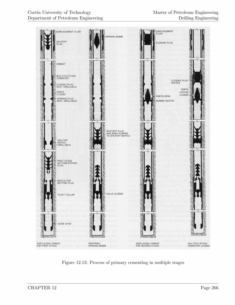
Curtin University of TechnologyDepartment of Petroleum Engineering
Master of Petroleum EngineeringDrilling Engineering
Figure 12.13: Process of primary cementing in multiple stages
CHAPTER 12 Page 266
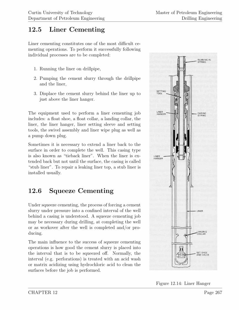
Curtin University of TechnologyDepartment of Petroleum Engineering
Master of Petroleum EngineeringDrilling Engineering
12.5 Liner Cementing
Figure 12.14: Liner Hanger
Liner cementing constitutes one of the most difficult ce-menting operations. To perform it successfully followingindividual processes are to be completed:
1. Running the liner on drillpipe,
2. Pumping the cement slurry through the drillpipeand the liner,
3. Displace the cement slurry behind the liner up tojust above the liner hanger.
The equipment used to perform a liner cementing jobincludes: a float shoe, a float collar, a landing collar, theliner, the liner hanger, liner setting sleeve and settingtools, the swivel assembly and liner wipe plug as well asa pump down plug.
Sometimes it is necessary to extend a liner back to thesurface in order to complete the well. This casing typeis also known as “tieback liner”. When the liner is ex-tended back but not until the surface, the casing is called“stub liner”. To repair a leaking liner top, a stub liner isinstalled usually.
12.6 Squeeze Cementing
Under squeeze cementing, the process of forcing a cementslurry under pressure into a confined interval of the wellbehind a casing is understood. A squeeze cementing jobmay be necessary during drilling, at completing the wellor as workover after the well is completed and/or pro-ducing.
The main influence to the success of squeeze cementingoperations is how good the cement slurry is placed intothe interval that is to be squeezed off. Normally, theinterval (e.g. perforations) is treated with an acid washor matrix acidizing using hydrochloric acid to clean thesurfaces before the job is performed.
CHAPTER 12 Page 267
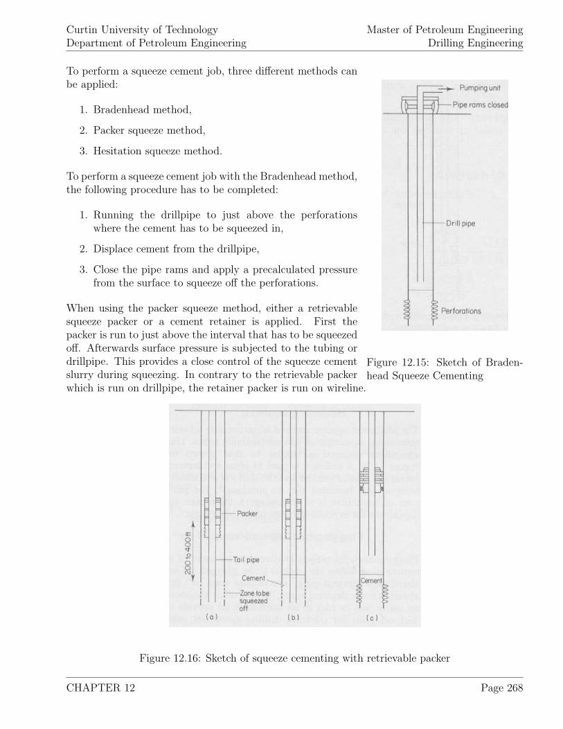
Curtin University of TechnologyDepartment of Petroleum Engineering
Master of Petroleum EngineeringDrilling Engineering
Figure 12.15: Sketch of Braden-head Squeeze Cementing
To perform a squeeze cement job, three different methods canbe applied:
1. Bradenhead method,
2. Packer squeeze method,
3. Hesitation squeeze method.
To perform a squeeze cement job with the Bradenhead method,the following procedure has to be completed:
1. Running the drillpipe to just above the perforationswhere the cement has to be squeezed in,
2. Displace cement from the drillpipe,
3. Close the pipe rams and apply a precalculated pressurefrom the surface to squeeze off the perforations.
When using the packer squeeze method, either a retrievablesqueeze packer or a cement retainer is applied. First thepacker is run to just above the interval that has to be squeezedoff. Afterwards surface pressure is subjected to the tubing ordrillpipe. This provides a close control of the squeeze cementslurry during squeezing. In contrary to the retrievable packerwhich is run on drillpipe, the retainer packer is run on wireline.
Figure 12.16: Sketch of squeeze cementing with retrievable packer
CHAPTER 12 Page 268
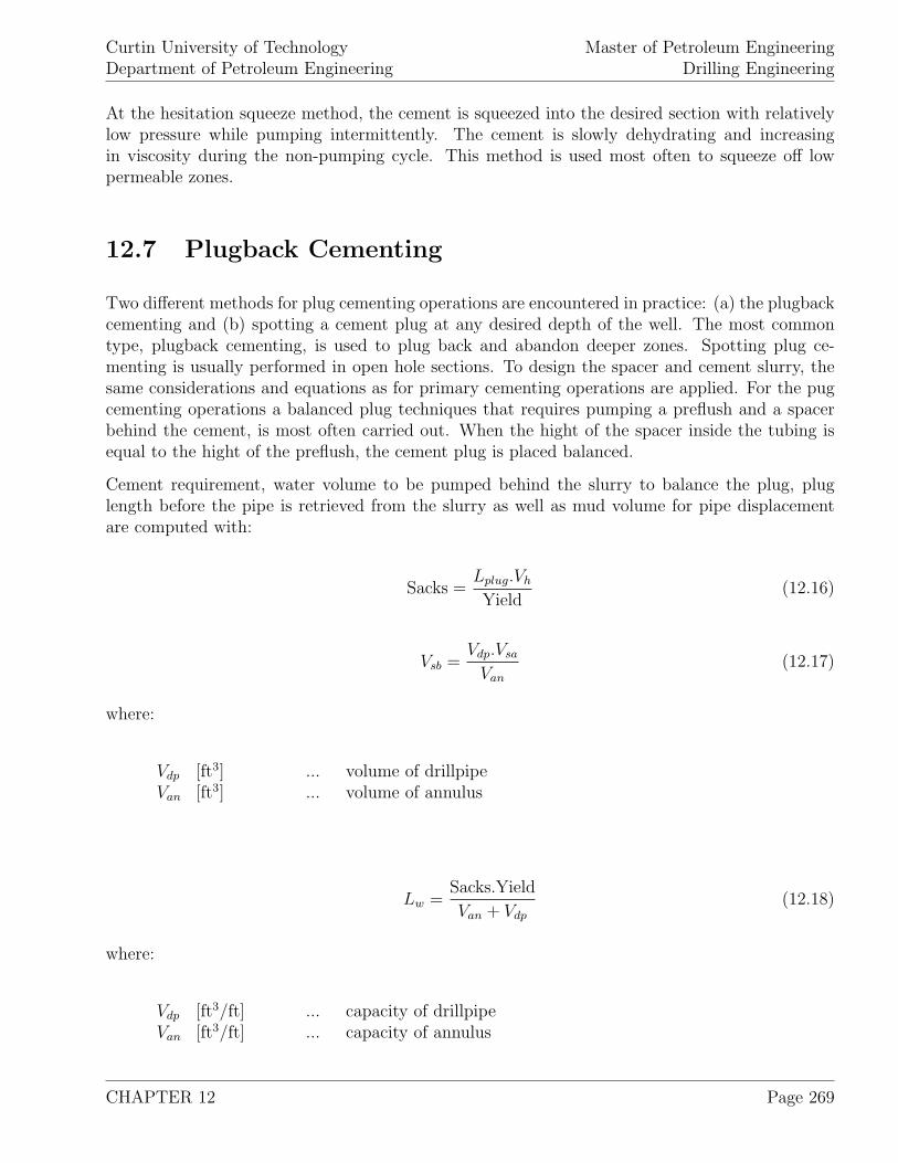
Curtin University of TechnologyDepartment of Petroleum Engineering
Master of Petroleum EngineeringDrilling Engineering
At the hesitation squeeze method, the cement is squeezed into the desired section with relativelylow pressure while pumping intermittently. The cement is slowly dehydrating and increasingin viscosity during the non-pumping cycle. This method is used most often to squeeze off lowpermeable zones.
12.7 Plugback Cementing
Two different methods for plug cementing operations are encountered in practice: (a) the plugbackcementing and (b) spotting a cement plug at any desired depth of the well. The most commontype, plugback cementing, is used to plug back and abandon deeper zones. Spotting plug ce-menting is usually performed in open hole sections. To design the spacer and cement slurry, thesame considerations and equations as for primary cementing operations are applied. For the pugcementing operations a balanced plug techniques that requires pumping a preflush and a spacerbehind the cement, is most often carried out. When the hight of the spacer inside the tubing isequal to the hight of the preflush, the cement plug is placed balanced.
Cement requirement, water volume to be pumped behind the slurry to balance the plug, pluglength before the pipe is retrieved from the slurry as well as mud volume for pipe displacementare computed with:
Sacks =Lplug.Vh
Yield(12.16)
Vsb =Vdp.Vsa
Van
(12.17)
where:
Vdp [ft3] ... volume of drillpipeVan [ft3] ... volume of annulus
Lw =Sacks.Yield
Van + Vdp
(12.18)
where:
Vdp [ft3/ft] ... capacity of drillpipeVan [ft3/ft] ... capacity of annulus
CHAPTER 12 Page 269
Curtin University of TechnologyDepartment of Petroleum Engineering
Master of Petroleum EngineeringDrilling Engineering
Vmd = (Ldp − Lw) .Vdp − Vsb (12.19)
where:
Vdp [bbl/ft] ... capacity of drillpipeLplug [ft] ... length of desired plugVh [ft3/ft] ... capacity of holeVsa [bbl] ... spacer volume ahead of slurryVsb [bbl] ... spacer volume behind of slurryVmd [bbl] ... volume of mud to displace pipe
CHAPTER 12 Page 270
Curtin University of TechnologyDepartment of Petroleum Engineering
Master of Petroleum EngineeringDrilling Engineering
12.8 Examples
1. Cement Class A containing 4 % bentonite is to be mixed. The normal water content of ClassA cement is 46 %, for each added percent of bentonite, 5.3 % of water has to be added. Thespecific gravities of cement and bentonite are found to be 3.13 and 2.65 respectively. The weightof bentonite, the total percent of water to be added as well as the volume of water to be mixedwith one sack of cement, the slurry yield and the slurry density have to be computed.
2. A 7 [in], 29 [lb/ft], N-80 casing has to be cemented in a 9.75 [in] hole for the length of 9,000 [ft].A 60 [ft] shoe track is to be used and cementing carried out with a Class G, 15.4 [ppg] cement. Theplastic viscosity and the yield point of the cement are 50 [cp] and 10 [lb/ 100 ft] respectively. Thecement is pumped with a duplex pump, having a 18 [in] stroke, a 6.5 [in] liner and a 2.5 [in] rod,and is operating at 60 [rpm] with an efficiency of 90 %. The water requirement of Class G cementis 5 [gal/sack] with the slurry volume of 1.15 [ft3/sack]. Since the cement is to be prevented fromcontamination with the previously used 11.6 [ppg] drilling mud, 30 [bbl] of fresh water are pumpedas preflush spacer. For cement mixing, a truck with a mixing capacity of 30 [sacks/min] is used.Calculate the:
(a) Quantity of cement required,(b) Volume of mixing water,(c) Total time for the job, allowing 15 minutes for
the release of plug,(d) Pressure differential prior to pumping the plug,(e) Flow velocity in the casing and the type of flow,(f) Flow velocity in the annulus and the type of flow.
3. A 5 [in] OD, 18 [lb/ft] liner (including hanger and float) is to be cemented in a 6-14
[in] hole fora length of 2,000 [ft]. The liner is run in on a 2-7
8[in], 10.4 [lb/ft] drillpipe to the liner landing
collar at 11,540 [ft]. The total well depth is 11,600 [ft], the liner-wipe plug at 9,615 [ft] and thetop of the liner at 9,600 [ft]. Calculate the:
(a) Sacks of Class E cement required if theyield is 1.15 [ft3/sack],
(b) Displacement to the liner plug,(c) Displacement from the liner plug to the landing collar.
4. Within a 6-12
[in] hole a 300 [ft] plug is to be placed at 9,000 [ft] using a 2-38
[in], 4.6 [lb/ft]tubing. When 15 [bbl] of water are to be pumped ahead of the slurry that has a yield of 1.5[ft3/sack], compute the:
CHAPTER 12 Page 271

Curtin University of TechnologyDepartment of Petroleum Engineering
Master of Petroleum EngineeringDrilling Engineering
(a) Sacks of cement required,(b) Volume of water to be pumped behind the slurry,(c) Amount of mud required to displace the spacer
to the balanced point.
CHAPTER 12 Page 272
Curtin University of TechnologyDepartment of Petroleum Engineering
Master of Petroleum EngineeringDrilling Engineering
Bibliography
[1] Aadnoy B.S., “Modern Well Design”, A.A Balkema, Rotterdam, (1996), 240 pages.
[2] Baker R., “A Primer of Oil-Well Drilling, Fourth Edition”, Petroleum Extension Ser-vice, University of Texas, Austin TX, (1979), 94 pages.
[3] Baker R., “A Primer of Offshore Operations, Second Edition”, Petroleum ExtensionService, University of Texas, Austin TX, (1985), 114 pages.
[4] Bourgoyne A.T. Jr., Millheim K.K., Chenevert M.E., Young F.S., “Applied Drilling En-gineering”, SPE Textbook Series, Vol 2, (1991), 502 pages.
[5] Craft B.C., Holden W.R., Graves E.D., “Well Design: Drilling and Production”,Prentice-Hall Inc., Englewood Cliffs New Jersey, (1962), 571 pages.
[6] Darley H.C.H., Gray G.R., “Composition and Properties of Drilling and CompletionFluids, Fifth Edition”, Gulf Publishing Company, Houston TX, (1988), 643 pages.
[7] Devereux S., “Drilling Technology in nontechnical language”, PennWell Publishing,Tulsa Oklahoma, (1999), 337 pages.
[8] Earlougher R.C. Jr., “Advances in Well Test Analysis”, Monograph Volume 5 of theHenry L. Doherty Series, (1977), 264 pages.
[9] Economides M.J., Watters L.T., Dunn-Norman S., “Petroleum Well Construction”, JohnWiley & Sons Publishing, (1998), 622 pages.
[10] ETA Offshore Seminars, Inc. “The Technology of Offshore Drilling, Completion andProduction”, The Petroleum Publishing Company, Tulsa Oklahoma, (1976), 426 pages.
[11] Gabolde G., Nguyen J.-P., “Drilling Data Handbook, Sixth Edition”, Institut Francaisdu Petrole, Gulf Publishing Company, Houston TX, (1991), 533 pages.
[12] Hallibuton, “Technology Exchange Session, 1992”, (1992).
[13] Harris L.M., “An Introduction to Deepwater Floating Drilling Operations”, PPEBooks, Petroleum Publisjinh Company, Tulsa Oklahoma, (1972), 272 pages.
[14] Hughes Tool Company, “Drilling Manual”, Section B, care, handling & specifications fortool joints, drill pipe, casing & tubing, (1969),
CHAPTER 12 Page 273
Curtin University of TechnologyDepartment of Petroleum Engineering
Master of Petroleum EngineeringDrilling Engineering
[15] Lapeyrouse N.J., “Formulas and Calculations for Drilling, Production andWorkover”, Gulf Publishing Company, Houston TX, (1992), 216 pages.
[16] Maurer W.C., “Advanced Drilling Techniques”, Petroleum Publishing Company, TulsaOklahoma, (1980), 698 pages.
[17] Mian M.A., “Petroleum Engineering Handbook For The Practicing Engineer, VolII”, PennWell Publishing, Tulas Oklahoma, (1992), pp. 271-453.
[18] Mitchell B., “Advanced Oilwell Drilling Engineering Handbook”, Oilwell Drilling,Golden Colorado, (1974), 605 pages.
[19] Moore P.L., “Drilling Practices Manual, Second Edition”, PennWell Publishing, TulsaOklahoma, (1986), 586 pages.
[20] Mouchet J.P., Mitchell A., “Abnormal pressures while drilling, Origins - Predictions- Detection - Evaluation”, elf aquitaine, manuels techniques 2, (1989), 255 pages.
[21] Short J.A., “Drilling and Casing Operations”, PennWell Publishing, Tulsa Oklahoma,(1982), 426 pages.
[22] Short J.A., “Prevention, Fishing & Casing Repair”, PennWell Publishing, Tulsa Okla-homa, (1995), 559 pages.
[23] SPE Reprint Series, “Well Completions”, No. 5, (1970), 41 articles, 344 pages.
[24] SPE Reprint Series, “Drilling”, No. 22, (1987), 33 articles, 348 pages.
[25] SPE Reprint Series, “Directional Drilling”, No. 30, (1990), 23 articles, 208 pages.
[26] SPE Reprint Series, “Coiled-Tubing Technology”, No. 38, (1994), 20 articles, 176 pages.
[27] Whittaker A., “Mud Logging Handbook”, Prentice Hall, Englewood Cliffs New Jersey,(1991), 531 pages.
CHAPTER 12 Page 274


![]HSPK MYVT L [YH VMM - sears.com · mhzopvu puzpkly whzz]hspk myvt l_[yh vmm yln\shy huk zhsl wypjlk hwwhyls mvv[^lhy hjjlzzvyplz [l_[ mhss [v mvy `v\y vmm whzz](https://img.pdfslide.us/doc/110x75/5d273df988c993b7508c09d3/hspk-myvt-l-yh-vmm-searscom-mhzopvu-puzpkly-whzzhspk-myvt-lyh-vmm-ylnshy.jpg)


![Ihykgbl evgZyaZibkdZ - uCozkremjanoe.ucoz.ru/2019...russkij_jazyk_9_klass.pdf · 6 Bkihevamyj_ijh^mdpbbdZjlbgba\_klguoom^h`gbdh\gZmjhdZojmkkdh]hyaudZ mqbl_ev hibjZ_lky gZ l_ agZgby](https://img.pdfslide.us/doc/110x75/5f377f03b6d95c51ee556103/ihykgbl-evgzyazibkdz-6-bkihevamyjijhmdpbbdzjlbgbaklguoomhgbdhgzmjhdzojmkkdhhyaudz.jpg)