Space-Time Observation

of Brain Actvity

Brian D. Ripley

Professor of Applied StatisticsUniversity of Oxford

ripley@stats.ox.ac.uk

http://www.stats.ox.ac.uk/∼ripley/talks.html

Outline

Joint work with Jonathan Marchini (as a D.Phil student).

Part 1: Magnetic Resonance Imaging of Brain Structure

Data, background and advice provided by Peter Styles (MRC Biochemicaland Clinical Magnetic Resonance Spectroscopy Unit, Oxford)

Part 2: Statistical Analysis of Functional MRI Data

Data, background and advice provided by Stephen Smith (Oxford Centrefor Functional Magnetic Resonance Imaging of the Brain) and Nick Lange(McLean Hospital, Harvard).

Magnetic Resonance Imaging

Magnetic resonance imaging is a non-invasive way of examining a livingbrain as it functions. We will only consider human brains, but work is alsodone on rat brains, which are smaller and can be given more interference.

In MRI can trade temporal, spatial and spectral resolution. Data is acquiredin Fourier domain over a period, down to around 3 seconds. The subjectis immersed in a strong magnetic field (needs powerful magnets—that inOxford is 3 Tesla) and responses to input signals allow information to becollected simultaneously spatially. The sorts of information are

• spin decay rates of hydrogen atoms, longitudinally and transversally(T1 and T2).

• BOLD, measurements of presence of oxygenated blood.

• perfusion of blood.

• presence of specific chemicals.

Collect one or more over ca 45 minutes in the scanner.

Data rates

A typical experiment will collect information on up to 256×256×30 voxels.This could be collected at up to 200 time points, and on several quantities.

Typically one experiment yields 1–100 million observations. There are bea few hundred sessions (a few on up to 100 subjects) in the course of amedical/psychological/drug study.

Data collection is expensive, especially on research machines.

More ‘powerful’ machines are also more unreliable, and may produce lessprecise results than production machines unless very well tuned.

Part 1:

MRI Studies of Brain Structure

Neurological Change

Interest is in the change of tissue state and neurological function aftertraumatic events such as a stroke or tumour growth and removal. The aimhere is to identify tissue as normal, impaired or dead, and to compare imagesfrom a patient taken over a period of several months.

In MRI can trade temporal, spatial and spectral resolution. In MR spec-troscopy the aim is a more detailed chemical analysis at a fairly low spatialresolution. In principle chemical shift imaging provides a spectroscopicview at each of a limited number of voxels: in practice certain aspects ofthe chemical composition are concentrated on.

Pilot Study

Our initial work has been exploring ‘T1’ and ‘T2’ images (the conventionalMRI measurements) to classify brain tissue automatically, with the aimof developing ideas to be applied to spectroscopic measurements at lowerresolutions.

Consider image to be made up of ‘white matter’, ‘grey matter’, ‘CSF’(cerebro–spinal fluid) and ‘skull’.

Initial aim is reliable automatic segmentation. Since applied to a set ofpatients recovering from severe head injuries.

Some Data

T1 (left) and T2 (right) MRI sections of a ‘normal’ human brain.

This slice is of 172 × 208 pixels. Imaging resolution was 1 x 1 x 5 mm.

Data from the same image in T1–T2 space.

Imaging Imperfections

The clusters in the T1–T2 plot were surprising diffuse. Known imperfec-tions were:

(a) ‘Mixed voxel’ / ‘partial volume’ effects. The tissue within a voxel maynot be all of one class.

(b) A ‘bias field’ in which the mean intensity from a tissue type varies acrossthe image. This effect is thought to vary approximately multiplicativelyand to consist of a radial component plus a linear component, the lattervarying from day to day.

(c) The ‘point spread function’. Because of bandwidth limitations in theFourier domain in which the image is acquired, the true observed imageis convolved with a spatial point spread function of ‘sinc’ (sin x/x) form.The effect can sometimes be seen at sharp interfaces (most often theskull / tissue interface) as a rippling effect, but is thought to be small.

Bias Fields

There is an extensive literature on bias field correction. One approach usesa stochastic process prior for the bias field, and is thus another re-inventionof the ideas known as kriging in the geostatistical literature. Based onexperience with the difficulty of choosing the degree of smoothing and thelack of resistance to outliers (kriging is based on assumptions of Gaussianprocesses) we prefer methods with more statistical content and control.

Our basic model is

log Yij = µ + βclass(ij) + s(i, j) + εij

for the intensity at voxel (i, j), studied independently for each of the T1 andT2 responses. Here s(x, y) is a spatially smooth function.

Of course, the equation depends on the classification, which will itselfdepend on the predicted bias field. This circularity is solved by iterativeprocedure, starting with no bias field.

Estimation

If the classification were known we would use a robust method that fits along-tailed distribution for εij, unconstrained terms αj for each class, anda ‘smooth’ function s. We cope with unknown class in two ways. In theearly stages of the process we only include data points whose classificationis nearly certain, and later we use

log Yij = µ +∑

class c

βc p(c |Yij) + s(i, j) + εij

that is, we average the class term over the posterior probabilities for thecurrent classification.

For the smooth term s we initially fitted a linear trend plus a spline model inthe distance from the central axis of the magnet, but this did not work well,so we switched to loess. Loess is based on fitting a linear surface locallyplus approximation techniques to avoid doing for the order of 27 000 fits.

Fits of bias fields

Fitted ‘bias fields’ for T1 (left) and T2 (right) images.

The bias fields for these images are not large and change intensity by 5–10%.

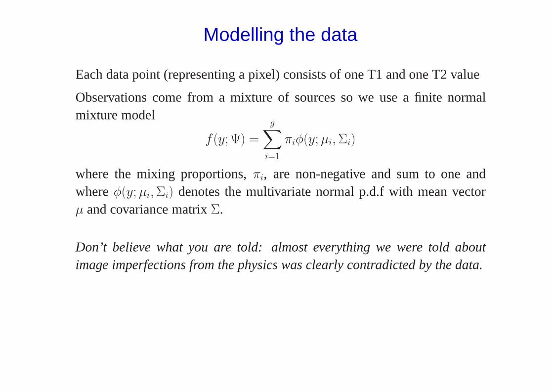
Modelling the data

Each data point (representing a pixel) consists of one T1 and one T2 value

Observations come from a mixture of sources so we use a finite normalmixture model

f(y; Ψ) =

g∑

i=1

πiφ(y; µi, Σi)

where the mixing proportions, πi, are non-negative and sum to one andwhere φ(y; µi, Σi) denotes the multivariate normal p.d.f with mean vectorµ and covariance matrix Σ.

Don’t believe what you are told: almost everything we were told aboutimage imperfections from the physics was clearly contradicted by the data.

Application/Results

6 component model

• CSF

• White matter

• Grey matter

• Skull type 1

• Skull type 2

• Outlier component (fixed mean and large variance)

Initial estimates chosen manually from one image and used in the classifi-cation of other images.

A Second Dataset

T1 (left) and T2 (right) MRI sections of another ‘normal’ human brain.

Classification image (left) and associated T1/T2 plot (right), training the 6-component

mixture model from its fit on the reference subject.

Outliers and anomalies

We have found our scheme to be quite robust to variation in imagingconditions and to different ‘normal’ subjects. The ‘background’ class helpsgreatly in achieving this robustness as it ‘mops up’ the observations whichdo not agree with the model.

However, outliers can be more extreme:

T1–T2 plot of a brain slice of a brain with a pathology.

This illustrates the dangers of classifying all the points. This is a particularlycommon mistake when neural networks are used for classification, and wehave seen MRI brain scans classified by neural networks where commonsense suggested an ‘outlier’ report was the appropriate one.

The procedure presented here almost entirely ignores the spatial nature ofthe image. For some purposes this would be a severe criticism, as contextualclassification would be appropriate. However, our interest in these imagesis not a pretty picture but is indeed in the anomalies, and for that we preferto stay close to the raw data. The other interest is in producing summarymeasures that can be compared across time.

Part 2:

Statistics of Functional MRI Data

‘Functional’ Imaging

Functional PET (positron emission spectroscopy: needs a cyclotron) andMRI are used for studies of brain function: give a subject a task and seewhich area(s) of the brain ‘light up’.

Functional studies were done with PET in the late 1980s and early 1990s,now fMRI is becoming possible. Down to 1 × 1 × 3 mm voxels.

PET has lower resolution, and relies on injecting agents into the bloodstream. Comparisons are made between PET images in two states (e.g.‘rest’ and ‘stimulus’) and analysis is made on the difference image. PETimages are very noisy, and results are averaged across several subjects.

fMRI has a higher spatial and temporal resolution. So most commonlystimuli are applied for a period of 10–30 secs, images taken around every 3secs, with several repeats of the stimulus being available for one subject.

The commonly addressed statistical issue is ‘has the brain state changed’,and if so where?

Left: A pain experiment. Blue before drug administration, green after, yellow both.

Right: A verbal/spatial reasoning test, averaged over 4 subjects. 12 slices, read row-

wise from bottom of head to top. Blue=spatial, red=verbal.

Experimental Design Issues

Some stimuli are not amenable to the ‘box-car’ approach. For example, painexperiments. So there are so-called single-event designs with deterministicor random intervals (to avoid subject anticipation).

What is actually observed, the BOLD effect, is both delayed and blurred bythe haemodynamic response function. It is thought that the haemodynamicresponse occurs over 10 secs or so; this limits the temporal resolution.

Need to design these experiments much more carefully than is usual.

Perfectly possible to do more than one experiment at once, e.g. 30 secsperiod for visual stimulation, 45 secs period for auditory stimulation.

Time (seconds)

Res

pons

e

0 50 100 150 200 250 300

850

900

950

1000

1050

A real response (solid line) from a 100-scan (TR=3sec) dataset in an area of activationfrom the visual experiment. The periodic boxcar shape of the visual stimulus is shown

below.

SPM

‘Statistical Parametric Mapping’ is a widely used program and methodol-ogy of Friston and co-workers, originating with PET. The idea is to map‘t-statistic’ images, and to set a threshold for statistical significance.

The t-statistic is in PET of a comparison between states over a number ofsubjects, voxel by voxel. Thus the numerator is an average over subjectsof the difference in response in the two states, and the denominator is anestimate of the standard error of the numerator.

The details differ widely between studies, in particular if a pixel-by-pixel orglobal estimate of variance is used.

The details also vary widely between releases of and users of the programs.

Example PET Statistics Images

From Holmes et al (1996). 12 subjects, 6 A–B, 6 B–A.

Mean difference image. Voxel-wise variance image.

Voxel-wise t–statistic image.

Smoothed variance image. Resulting t–statistic image.

The GLM approach

A SAS-ism: it means linear models. May take the autocorrelation of thenoise (in time) into account.

• May or may not remove overall mean.

• May or may not remove trends.

• Design matrix may contain

– An overall mean

– A linear or other trend

– The signal convolved with a linearly-parametrized HRF: often acouple of gammas or a gamma density and its derivative.

• The signal is usually filtered by a matrix S, so the model becomes

SY = SXβ + Sε, ε ∼ N(0, σ2V (θ))

Variations on the theme in a series of papers by Friston et al:

Analysis of functional MRI time-series

Analysis of functional MRI time-series revisited

Analysis of functional MRI time-series revisited—again

All fit β by least-squares, but differ in the estimate used of σ2. The thirdpaper suggests a scaled version of the residual MSq.

Not exactly unknown statistical theory (to statisticians)!

Two main issues:

1. What is the best estimate β̂ of β?

2. What is a good (enough) estimate of its null-hypothesis variability,var(β̂)?

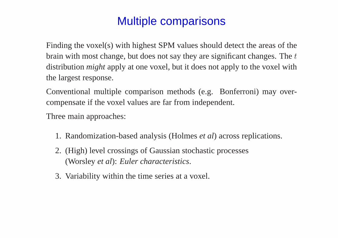
Multiple comparisons

Finding the voxel(s) with highest SPM values should detect the areas of thebrain with most change, but does not say they are significant changes. The t

distribution might apply at one voxel, but it does not apply to the voxel withthe largest response.

Conventional multiple comparison methods (e.g. Bonferroni) may over-compensate if the voxel values are far from independent.

Three main approaches:

1. Randomization-based analysis (Holmes et al) across replications.

2. (High) level crossings of Gaussian stochastic processes(Worsley et al): Euler characteristics.

3. Variability within the time series at a voxel.

Randomization-based Statistics

Classical statistical inference of designed experiments is based on the uncer-tainly introduced by the randomization, and not on any natural variability.

A typical fPET or fMRI experiment compares two states, say A and B. Ifthere is no difference between the states we can flip the labels within eachpair (for each subject in PET, for each repetition × subject in fMRI). Ifthere are n pairs, there are 2n possible A–B or B–A labellings. If there isno difference, these all give equally likely values of an observed statistic, socompared observed statistic to the permutation distribution.

Can choose any statistic one can compute fairly easily.

Holmes et al. actually used a restricted randomization, keep the balance oftheir 12 pairs into 6 A–B and 6 B–A pairs.

Euler Characteristics

The Worsley et al approach is based on modelling the SPM image Xijk

as a Gaussian (later relaxed) stochastic process in continuous space witha Gaussian autocorrelation function (possibly geometrically anisotropic).The autocorrelation function must be estimated from the data, but to someconsiderable extent is imposed by low-pass filtering.

For such processes there are results (Hasofer, Adler) on the level sets{x : X(x) > x0}. These will be made up of components, themselves con-taining holes. The results are on the expected Euler characteristic (numberof sets minus holes) as function of x0, but for large x0 there is a negligibleprobability of a hole, and the number is approximately Poisson distributed.Thus we can choose x0 such that under the null hypothesis

P (X(x) > x0 for any x ∈ A) ≈ 5%

Note that this is based on variability within a single image to address themultiple comparisons point.

Time-Series-based Statistics

The third component of variability is within the time series at each voxel.Suppose there were no difference between A and B. Then we have astationary autocorrelated time series, and we want to estimate its mean andthe standard error of that mean.

This is a well-known problem in the output analysis of (discrete-event)simulations.

More generally, we want the mean of the A and B phases, and there willbe a delayed response (approximately known) giving a cross-over effect.Instead, use a matched filter (sin wave?) to extract effect, and estimatedautocorrelations (like Hannan estimation) or spectral theory to estimatevariability. For a sin wave the theory is particularly easy: the log absolutevalue of response has a Gumbel distribution with location depending on thetrue activation.

fMRI Example

Data on 64 × 64 × 14 grid of voxels. (Illustrations omit top and bottomslices and areas outside the brain, all of which show considerable activity,probably due to registration effects.)

A series of 100 images at 3 sec intervals: a visual stimulus (a striped pattern)was applied after 30 secs for 30 secs, and the A–B pattern repeated 5 times.In addition, an auditory stimulus was applied with 39 sec ‘bursts’.

Conventionally the images are filtered in both space and time, both high-pass time filtering to remove trends and low-pass spatial filtering to reducenoise (and make the Euler characteristic results valid). The resulting t–statistics images are shown on the next slide. These have variances estimatedfor each voxel based on the time series at that voxel.

SPM99 t–statistic images, with spatial smoothing on the right

Slice 5, with spatial smoothing on the right

A Closer Look at some Data

A 10 × 10 grid in an area of slice 5 containing activation.

Alternative Analyses

• Work with raw data.

• Non-parametric robust de-trending, Winsorizing if required.

• Work in spectral domain.

• Match a filter to the expected pattern of response (square wave input,modified by the haemodynamic response).

• Non-parametric smooth estimation of the noise spectrum at a voxel,locally smoothed across voxels.

• Response normalized by the noise variance should be Gumbel (withknown parameters) on log scale.

This produced much more extreme deviations from the background varia-tion, and much more compact areas of response. 30–100 minutes for a brain(in S / R on ca 400MHz PC).

Log abs filtered response, with small values coloured as background (red). Threshold

for display is p < 10−5 (and there are ca 20,000 voxels inside the brain here).

Trend-removal

Time (seconds)

Res

pons

e

0 50 100 150 200 250 300

440

460

480

500

520

540

A voxel time series from the dataset showing an obvious non-linear trend.

We used a running-lines smoother rejecting outliers (and Winsorizing theresults).

−4 −3 −2 −1 0 1 2

0.0

0.2

0.4

0.6

0.8

log10(response)

Histogram of log filtered response, for an image with activation.

We can validate the distribution theory by looking at frequencies withoutstimulus, and ‘null’ images.

Plotting p values

p-value image of slice 5thresholded to showp-values below 10−4 andoverlaid onto an image ofthe slice. Colours indicatedifferential responseswithin each cluster. Anarea of activation is shownin the visual cortex, as wellas a single ‘false-positive’,that occurs outside of thebrain.

10−4

10−5

10−6

10−7

10−8

10−9

10−10

Calibration

Before we worry about multiple comparisons, are the t-statistics (nearly)t-distributed?

Few people have bothered to check, and those who did (Bullmore, Brammeret al, 1996) found they were not.

We can use null experiments assome sort of check.In our analysis we can use otherfrequencies to self-calibrate, butwe don’t need to:

x

-log(

1-F

(x))

0 5 10 15

05

1015

0-2

-4-6

-8P

-val

ue (

pow

ers

of 1

0)

Bullmore et al.

Empirical

The

oret

ical

100 10−1 10−2 10−3 10−4 10−5 10−6

100

10−1

10−2

10−3

10−4

10−5

10−6

AR(1) + non−linear detrending

Empirical

The

oret

ical

100 10−1 10−2 10−3 10−4 10−5 10−6

100

10−1

10−2

10−3

10−4

10−5

10−6

SPM99

Empirical

The

oret

ical

100 10−1 10−2 10−3 10−4 10−5 10−6

100

10−1

10−2

10−3

10−4

10−5

10−6

This paper

Empirical

The

oret

ical

100 10−1 10−2 10−3 10−4 10−5 10−6

100

10−1

10−2

10−3

10−4

10−5

10−6

Conclusions

• Look at your data (even if it is on this scale: millions of points perexperiment).

• Data ‘cleaning’ is vital for routine use of such procedures.

• Fit your theory to your analysis, not vice versa.

• You need to be sure that the process is reliable, as no one can checkon this scale.

• There is no point in building sophisticated methods on invalid founda-tions.

• It is amazing what can be done in high-level languages on cheapcomputers.