Embed Size (px)
Citation preview

Natural Direct and Indirect E↵ects for Survival
Outcomes in a Complex Survey Setting
By:
Michael Reaume
Supervisor:
Dr. Michael A. McIsaac
Biostatistics Practicum Report
Department of Public Health Sciences
Queen’s University
(September 2017)

Acknowledgements
I would like to begin by thanking my supervisor, Dr. Michael McIsaac, for his ongoing
guidance and encouragement. Dr. McIsaac was extremely patient with me over the last
year, and he provided me with invaluable advice and suggestions every time we met. I
am grateful for the support that I received from Dr. Will Pickett, Dr. Colleen Davison,
and both of their students; I enjoyed our weekly lab group meetings, and I learned a lot
from them. I would also like to thank the members of my examining committee - Dr.
Dongsheng Tu and Dr. Wenyu Jiang - for reviewing my practicum and for their
valuable feedback. Finally, I would like to thank the faculty and sta↵ at the
Department of Public Health Sciences for their support.
Funding and Support
Dr. McIsaac’s research program is funded by a Sciences and Engineering Research
Council of Canada Discovery Grant (RGPIN-2016-04384). Michael Reaume was also
supported by Queen’s University Graduate Awards (Senator Frank Carrell Fellowship
and Graduate Research Assistant Fellowship).
This study relied on data held at the Institute for Clinical Evaluative Sciences (ICES),
which is funded by an annual grant from the Ontario Ministry of Health and Long-Term
Care (MOHLTC). The opinions, results and conclusions reported in this paper are those
of the authors and are independent from the funding sources. No endorsement by ICES
of the Ontario MOHLTC is intended or should be inferred. These datasets were linked
using unique encoded identifiers and analyzed at ICES-Queen’s University.

Acronyms
AFT . . . . . . . . . . Accelerated Failure Time
BMI . . . . . . . . . . Body Mass Index
BRR . . . . . . . . . . Balanced Repeated Replication
CCHS . . . . . . . . Canadian Community Health Survey
ICES . . . . . . . . . Institute for Clinical Evaluative Sciences
IPTW . . . . . . . . Inverse Probability of Treatment Weighting
NDE . . . . . . . . . Natural Direct E↵ect
NHANES . . . . National Health and Nutritional Examination Survey
NIE . . . . . . . . . . . Natural Indirect E↵ect
SRS . . . . . . . . . . Simple Random Sampling
TE . . . . . . . . . . . . Total E↵ect
ii
Contents
Acknowledgements i
Funding and Support i
Acronyms ii
Introduction 1
1 Background 3
1.1 Canadian Community Health Survey (CCHS) . . . . . . . . . . . . . . . 3
1.2 Complex Survey Sampling . . . . . . . . . . . . . . . . . . . . . . . . . . 4
1.3 Analyzing Complex Survey Data . . . . . . . . . . . . . . . . . . . . . . 8
1.3.1 Design-Based vs. Model-Based Analyses . . . . . . . . . . . . . . 8
1.3.2 Variance Estimation . . . . . . . . . . . . . . . . . . . . . . . . . 10
1.3.3 Combining Survey Cycles . . . . . . . . . . . . . . . . . . . . . . 13
1.4 Causal Mediation Analysis with Survival Data . . . . . . . . . . . . . . . 14
1.4.1 Mediation Analysis . . . . . . . . . . . . . . . . . . . . . . . . . . 14
1.4.2 Natural E↵ect Models . . . . . . . . . . . . . . . . . . . . . . . . 17
1.4.3 Natural E↵ect Models with Survival Data . . . . . . . . . . . . . 20
2 Natural E↵ect Models for Survival Outcomes in a Complex Survey Set-
ting 22
2.1 Introduction . . . . . . . . . . . . . . . . . . . . . . . . . . . . . . . . . . 22
2.2 Methods . . . . . . . . . . . . . . . . . . . . . . . . . . . . . . . . . . . . 23
2.3 Simulation Study . . . . . . . . . . . . . . . . . . . . . . . . . . . . . . . 26
2.3.1 Simulation Study Methods . . . . . . . . . . . . . . . . . . . . . . 26
2.3.2 Simulation Study Results . . . . . . . . . . . . . . . . . . . . . . 30
2.4 Case Study . . . . . . . . . . . . . . . . . . . . . . . . . . . . . . . . . . 39
2.5 Discussion . . . . . . . . . . . . . . . . . . . . . . . . . . . . . . . . . . . 44
A Simulating Proportional Hazards Model 48
B Natural Direct and Indirect E↵ects for Cox Model (Binary Mediator) 51
iii

C Natural Direct and Indirect E↵ects for Cox Model (Continuous Medi-
ator) 54
D Coverage Rates (Binary Mediator) 56
E Coverage Rates (Continuous Mediator) 60
F Simulation: Common Exposure, Rare Outcome (Binary Mediator) 65
G Simulation: Common Exposure, Rare Outcome (Continuous Mediator) 71
H Variance of Regression Coe�cients 77
iv
Introduction
Mediation analysis is commonly used to uncover pathways in a causal model
(VanderWeele, 2016). Mediation analysis consists of decomposing the causal relationship
between the exposure and the outcome into two separate pathways: the direct e↵ect
and the indirect e↵ect. The indirect e↵ect refers to the pathway that acts through the
mediator, while the direct e↵ect refers to the pathway that does not act through the
mediator (Richiardi et al., 2013). Causal mediation analysis is generally performed by
using the di↵erence method or the product method (VanderWeele, 2016). While these
techniques are easy to implement, they only provide meaningful estimates of the direct
and indirect e↵ects when 1) the mediator is continuous and normally distributed, 2) the
outcome is continuous and normally distributed, and 3) there is no interaction in the
regression model for the outcome (VanderWeele, 2016). In other settings, such as when
the outcome is a survival time variable, the product method and the di↵erence method
will generally produce di↵erent estimates of the direct and indirect e↵ects, and neither
one of these two estimates will have a causal meaning (VanderWeele, 2011). To address
this limitation, several techniques have been developed in recent years, such as the
method of natural e↵ect models (VanderWeele, 2011; Lange et al., 2012; VanderWeele,
2016). Compared to traditional approaches of performing mediation analysis, the
method of natural e↵ect models has the advantage of being very flexible; the same
methodology can be used to provide causal estimates of the natural direct and indirect
e↵ects with almost any type of mediator and outcome variables (Lange et al., 2012).
The method of natural e↵ect models was developed for data collected through simple
random sampling (SRS), which refers to sampling schemes where 1) all individuals in
the population have the same probability of being selected into the sample, and 2) all
pairs of individuals have the same probability of being selected into the sample
(Lumley, 2010). In practice, public health and social sciences research often involves
analyzing data collected from complex surveys, which are usually defined as surveys
that consist of sampling schemes with multiple levels of selection (Lumley, 2010). In
order to perform a fully design-based analysis, information from the complex survey’s
sampling scheme must be incorporated into the analysis (Little, 2004; Lee and
Forthofer, 2006; Lumley, 2010). To our knowledge, the implications of incorporating
1

design information from complex surveys into natural e↵ect models have never been
considered directly. In other words, it is not known how natural e↵ect models should be
tailored to complex survey settings in general. As a result, some studies have
incorporated design features into natural e↵ect models in an ad hoc manner, while
others have simply disregarded the design features altogether. The purpose of this
practicum was to identify the optimal methodology for estimating natural direct and
indirect e↵ects for survival outcomes in a complex survey setting.
The remainder of this report is divided into two chapters, which are structured as
follows. Chapter 1 provides necessary background information related to complex
surveys and causal mediation analysis. More specifically, Section 1.1 provides a brief
introduction to the Canadian Community Health Survey (CCHS), which is an annual
survey conducted by Statistics Canada that will serve as a motivating example
throughout this report. Section 1.2 introduces concepts related to complex sampling
schemes, while Section 1.3 considers the analysis of data collected from complex
surveys. Section 1.4 introduces causal mediation analysis techniques and the challenges
in applying these methods to survival data. Chapter 2 examines the use of natural
e↵ect models for survival outcomes in a complex survey setting. Section 2.2 presents the
various di↵erent methods of estimating natural direct and indirect e↵ects (and their
corresponding variances) in such settings, and Section 2.3 includes a simulation study
that compares the performance of these methods. Section 2.4 provides a practical
example by using natural e↵ect models to determine whether job stress is a mediator of
the relationship between shift work and diabetes in a cohort of CCHS participants.
Finally, Section 2.5 summarizes the findings of this report and provides general
recommendations.
2

1 Background
1.1 Canadian Community Health Survey (CCHS)
The CCHS is an annual cross-sectional survey of the Canadian population designed to
collect information regarding health determinants and health care utilization at the
national, provincial, and regional levels (Statistics Canada, 2017). The target
population consists of all individuals 12 years of age and older who live in a private
dwelling in any Canadian province or territory, with the exception of 1) individuals
living on a reserve or an Aboriginal settlement in one of the provinces, 2) members of
the Canadian Forces, and 3) the institutionalized population (Statistics Canada, 2017).
Prior to 2007, the CCHS was conducted over a 2-year period, and the results were
released at the end of each 2-year cycle. Since 2007, each cycle of the CCHS has been
conducted over a 1-year period, and the results are released annually (Statistics
Canada, 2017). The first CCHS surveys selected participants from three di↵erent
sampling frames: 1) an area frame, 2) a list frame of telephone numbers within the area
frame, and 3) a random digit dialling frame (Statistics Canada, 2002). In 2015,
Statistics Canada eliminated the latter two sampling frames. Instead of using three
di↵erent sampling frames, the CCHS now selects all adult participants through the area
frame, while children aged 12 to 17 are selected through a list generated by the
Canadian Child Tax Benefit (Statistics Canada, 2017).
To ensure that su�ciently large samples are collected from each province and health
region, the CCHS employs multiple levels of stratification during the design phase.
First, a fixed total sample size is divided amongst provinces and health regions. To do
so, each province is allocated a sample size that is proportional to its estimated
population (relative to that of the other provinces), and health regions are allocated a
sample size that is proportional to the square root of the health region’s estimated
population (relative to that of the other health regions within the province). Thus, a
health region of size n within a province of size N will be allocated a sample of
approximately S ⇥ NT⇥p
nN
individuals, where S is the fixed total sample size and T is
the estimated population of Canada. Once the samples sizes are allocated to each
health region, individuals are selected using a stratified multi-stage cluster sampling
3
scheme. The health regions are stratified by city type (major urban centre, city, rural
region), and the major urban centres are further stratified according to geographic
location and socioeconomic characteristics. To facilitate data collection, clusters of 150
to 250 dwellings are created on the basis of geographic location, and six clusters are
randomly selected from within each stratum (Statistics Canada, 2017). The sampling of
clusters is performed using probability proportional to size, which means that the
probability of selecting a cluster is proportional to the number of dwellings within each
cluster (Lumley, 2010). Finally, households are selected using systematic sampling, and
one or two individuals are randomly selected from each household according to
pre-determined age-based selection probabilities, which are designed to oversample
children and seniors (Statistics Canada, 2017).
Certain design characteristics, such as stratum membership, cluster membership, and
sampling weights, must be known in order to perform design-based analyses (Lumley,
2010). While Statistics Canada does release sampling weights, the CCHS dataset does
not provide stratum and cluster membership information. Instead, Statistics Canada
releases a set of 500 replicate weights, which are obtained by re-sampling n� 1 out of n
clusters from within each stratum with replacement. The samples obtained through this
re-sampling process are multiplied by the original sampling weight in order to obtain
replicate weights. Finally, the replicate weights are post-stratified, which means that
they are re-scaled and adjusted in order to ensure that they are representative of the
Canada population. The original sampling weight is also post-stratified using the same
method that is employed to post-stratify the replicate weights (Statistics Canada, 2017).
1.2 Complex Survey Sampling
Almost all studies in the field of public health involve measuring a parameter in a finite
population (Lee and Forthofer, 2006; Lumley, 2010). For example, a researcher may be
interested in measuring the prevalence of diabetes in each Canadian province in order to
determine which jurisdictions require additional funding for diabetes treatment. This
quantity could be calculated directly if the status of diabetes were known for each
individual living in Canada. Unfortunately, such information is not readily available,
and interviewing the entire Canadian population is not feasible. As a result, researchers
4

are often forced to collect information on a sample of the population. The most
elementary way of obtaining a probability sample is by SRS, where each individual in
the population has an equal selection probability and each pair of individuals has an
equal joint selection probability (Lumley, 2010). In other words, SRS implies that 1)
the probability of selecting individual i is the same as the probability of selecting
individual j for all individuals i, j in the survey population, and 2) the probability of
selecting individuals i and j is the same as the probability of selecting individuals k and
l for all individuals i 6= j and k 6= l in the survey population. Thus, if a sample of size n
is drawn using SRS, each potential sample of size n is equally likely to be selected. This
approach di↵ers from complex sampling schemes, which are usually defined as sampling
techniques that involve multiple levels of selection (Lumley, 2010), although some
authors consider all sampling strategies other than SRS to be complex (Lee and
Forthofer, 2006).
Most single-stage sampling schemes such as SRS require the complete sampling frame
to be known in advance, which limits their utility in practice as this information is
rarely known for large populations (Lee and Forthofer, 2006; Lumley, 2010). It may not
be desirable to use SRS even when the sampling frame is known due to practical and/or
economic considerations (Lumley, 2010). For instance, a simple random sample of the
Canadian population would include individuals from many di↵erent regions across
Canada; it could be di�cult to conduct in-person interviews with a sample that covers
such a wide geographic area without exhausting considerable resources. Data collection
can be simplified by selecting individuals within naturally existing groups in the
population. This approach is known as cluster sampling, and it can involve a single
level or multiple levels of sampling (Lee and Forthofer, 2006; Lumley, 2010). For
instance, a four-stage cluster sample could be obtained by first sampling census
divisions, then sampling cities within the selected census divisions, and then sampling
neighbourhoods within the selected cities. Finally, individuals could be sampled from
the selected neighbourhoods in the fourth stage of sampling, thereby ensuring that
sampled individuals live in close proximity to other sampled individuals. While cluster
sampling can reduce the costs associated with data collection, this approach generally
results in estimates with larger variances when compared to a sample of identical size
obtained through SRS (Lee and Forthofer, 2006; Lumley, 2010). This phenomenon
5

occurs because individuals in a cluster are likely to be more similar to one another than
are individuals selected in a simple random sample (Lee and Forthofer, 2006; Lumley,
2010).
Another type of sampling scheme that is commonly used in survey research is stratified
sampling. The underlying idea is straightforward; the population is divided into groups
(known as strata) based on information that is available for each individual in the
population, and samples are taken from each stratum. Stratified sampling has two
major advantages over SRS and cluster sampling. First, it can lead to a reduction in
sampling variance. The reason for this is analogous to that which explains the greater
uncertainty in cluster sampling; individuals in a stratum are likely to be more similar to
one another than are individuals selected in a simple random sample. Stratified
sampling includes individuals from all strata, which means that more information is
collected from the population (Lumley, 2010). Second, stratified sampling can be used
to oversample groups that would otherwise be underrepresented. This ensures that the
samples are large enough to obtain reliable estimates for sub-groups of interest (Lee and
Forthofer, 2006; Lumley, 2010). To illustrate this point, consider the example of a
researcher who wishes to measure the prevalence of diabetes in each Canadian province.
If the researcher took a simple random sample of 2,500 individuals across Canada,
which has a population of 36,286,425 (Statistics Canada, 2016), then the probability of
being selected into the sample would be approximately 1 in 15,000�since
2,50036,286,425 ⇡ 6.89⇥ 10�5 ⇡ 1
15,000
�. The expected number of individuals selected from
Prince Edward Island, which has a population of 148,649, would be 10 (Statistics
Canada, 2016). Such a small sample would produce unstable and unreliable estimates
at the provincial level. Similar issues could arise in cluster sampling, since there is no
mechanism to ensure that clusters are distributed across the entire population. If one of
the objectives is to measure the prevalence of diabetes in Canada at the provincial level,
it would be beneficial to stratify the population by geographic region. In practice,
stratified sampling is limited by the fact that the information used for stratification
must be known in advance for each individual in the population (Lee and Forthofer,
2006; Lumley, 2010). While information about geographic location is usually readily
available, other variables, such as health indicators, are less likely to be known prior to
sampling.
6
Cluster sampling and stratified sampling are common examples of design strategies that
give rise to complex surveys. Sampling strategies can be combined; for instance,
stratified cluster sampling is used by researchers who wish to exploit the beneficial
properties of both cluster sampling and stratified sampling. One of the most important
implications of complex sampling strategies is the unequal selection probability (Lee
and Forthofer, 2006). This characteristic of complex surveys can be illustrated through
the following example. Suppose a researcher wants to enrol 1,000 Canadians into a
study. In order to be able to perform analyses within each province, the researcher
stratifies the population on the basis of geographic location and selects 100 individuals
from each province (using SRS). Since the population of Ontario is greater than that of
Prince Edward Island, the probability of selecting an individual in Ontario will be
smaller than in Prince Edward Island (Statistics Canada, 2016). If a secondary aim of
the study is to compute summary statistics at the national level, the data can be
analyzed in a way that takes into account the di↵erent selection probabilities. This is
done by using sampling weights, which are defined as the inverse of the selection
probability (Lee and Forthofer, 2006; Lumley, 2010). In the previous example, the
sampling weight of individuals in Prince Edward Island, which has a population of
148,649, would be approximately 1,500�since 100
148,649 ⇡ 6.73⇥ 10�5 ⇡ 11,500
�, while the
sampling weight of individuals in Ontario, which has a population of 13,982,984, would
be approximately 140,000�since 100
13,982,984 ⇡ 7.15⇥ 10�6 ⇡ 140, 000; Statistics Canada
(2016)�. Sampling weights provide a measure of how many people in the population are
represented by each sampled individual; those with larger sampling weights represent a
larger portion of the population and, thus, have more impact on the results.
Stratification can also be performed during the analysis stage. This approach, which is
known as post-stratification, adjusts the sampling weights in a way that ensures that
the estimated populations totals agree with known population totals (Lumley, 2010).
To implement post-stratification, the population total for each combination of the
variables used to adjust the sampling weights must be known (Lumley, 2010). In
addition to making the sample more representative of the population, thereby
minimizing sampling bias due to non-coverage of the sampling frame, post-stratification
can also increase precision if there is a relationship between the post-stratification
variables and the parameter of interest (Lee and Forthofer, 2006; Lumley, 2010). Since
7
post-stratification requires the population totals to be known for each cross-classified
category of the post-stratification variable(s), this method can be di�cult to apply to
situations with multiple post-stratification variables. Other techniques, such as raking
and calibration, have been developed for such settings. Post-stratification, raking, and
calibration provide the same advantages and benefits as stratification does, with the
only exception being that these methods cannot ensure that enough information is
collected from underrepresented groups (Lumley, 2010). Furthermore, it may not be
desirable or even possible to use stratification during the design stage (Lee and
Forthofer, 2006; Lumley, 2010). First, a stratification method that is suitable for one
analysis may be inappropriate for another. Second, an approach that incorporates too
many stratification variables could be di�cult to carry out in practice. Third, it may
not be possible to stratify on the basis of individual-level auxiliary variables if the
proposed sampling scheme involves cluster sampling, where selection depends on
cluster-level variables (Lumley, 2010). Post-stratification can exploit information from
variables collected during the survey, and it can also be modified based on the
objectives of the analysis. In practice, stratification and post-stratification are usually
employed together (Lee and Forthofer, 2006; Lumley, 2010).
1.3 Analyzing Complex Survey Data
1.3.1 Design-Based vs. Model-Based Analyses
There are two broad frameworks for analyzing complex survey data (Little, 2004). The
first, which is known as design-based inference, attempts to describe the parameters
that exist within the finite population from which the sample is drawn. The finite
population is considered to be fixed, and the goal is to estimate the parameters that
would be obtained if the entire population were surveyed (as in a census). For this
reason, sampling weights, which are used to ensure that the sample is representative of
the population, should always be used in the context of design-based inferences. The
uncertainty in design-based inference arises from the fact that the sample is unlikely to
be perfectly representative of the population (Lee and Forthofer, 2006; Lumley, 2010).
If the entire finite population were surveyed (as in a census), it would not be necessary
to report variances and confidence intervals in a design-based analysis, since there
8

would not be any sampling variability. The other framework that is commonly
employed by survey researchers is known as model-based inference. This approach does
not assume that the sample is drawn from a finite population; instead, it assumes that
the finite population is drawn from an infinite superpopulation, which is generated from
a model with unknown parameters. The goal of model-based inference is to estimate
the parameters in this superpopulation model (Lee and Forthofer, 2006; Lumley, 2010).
Unlike the previous approach, analyses carried out using the model-based framework
should always report variances and confidence intervals since it is impossible to sample
the entire infinite superpopulation. In other words, the parameters in the target
population are considered to be fixed in design-based inference, while they are treated
as random variables in model-based inference. If the parameters of interest are
equivalent across di↵erent groups of the population, it is not necessary to ensure that
the sample is representative of the population (Lee and Forthofer, 2006; Lumley, 2010).
As a result, some model-based analyses can be performed by ignoring the sampling
weights (Little, 2004; Lee and Forthofer, 2006; Lumley, 2010). It is important to note
that design-based and model-based approaches as described above are not the only
methods available for analyzing complex survey data; hybrid analyses combine elements
from both design-based and model-based frameworks (Sterba, 2009).
Design-based analyses are generally preferred when interest lies in estimating summary
statistics, such as the population mean (Lee and Forthofer, 2006; Lumley, 2010). A
popular estimator in design-based inference is the Horvitz-Thompson estimator, which
yields an unbiased estimate of the population mean by summing the weighted
observations and dividing by the total number of observations (Little, 2004; Lumley,
2010). Summary statistics can also be obtained through weighted regression analyses
with ratio estimators (Lumley, 2010). Interestingly, such approaches produce
asymptotically unbiased estimates of the parameters that would have been obtained if
the entire finite population were surveyed, even when the regression models are
misspecified (Lumley, 2010). However, precision depends on model fit; when the model
is correctly specified and all assumptions are satisfied, ratio estimators can be much
more e�cient than those obtained with the Horvitz-Thompson estimator (Little, 2004;
Lumley, 2010). Regression analyses are also commonly used to uncover relationships
between variables. In the context of design-based inference, regression models must
9

always incorporate weights, since this implicitly includes the relevant design information
and ensures that the sample is representative of the population (Little, 2004; Lee and
Forthofer, 2006; Lumley, 2010). The incorporation of sampling weights can lead to a
reduction in bias if the sampling design is informative (Lee and Forthofer, 2006;
Lumley, 2010), which means that the selection probability depends on the outcome
variable after controlling for the other covariates included in the model (Little, 2004).
Since sampling weights are inversely proportional to the selection probability,
observations with smaller selection probabilities have a disproportionately larger
influence on the model fitting procedure, which leads to instability and to a reduction in
precision. Estimates from unweighted regression analyses can be more precise than
those from weighted regression analyses, but they will be biased if the sampling design
is informative. If the sampling procedure depends on a set of auxiliary variables, then
these auxiliary variables can be included in model-based analyses (Lee and Forthofer,
2006; Lumley, 2010). However, some surveys do not release all information related to
the sampling design due to privacy concerns, which means that it may not be possible
to control for all relevant design variables. To address the trade-o↵ between bias and
precision, it is generally recommended to perform both weighted and unweighted
analyses. The results from both analyses can be compared, and any discrepancies
should be further investigated (Lee and Forthofer, 2006; Lumley, 2010). Some authors
recommend selecting the weighted model unless the increase in variance is too large
(Lee and Forthofer, 2006), while others believe that the unweighted model should be
used as long as the point estimates do not di↵er considerably from those of the weighted
model (Lumley, 2010). The underlying principle of these two approaches is the same;
both assume that the model with sampling weights has less bias, while the model
without sampling weights has greater precision.
1.3.2 Variance Estimation
Unbiased point estimates of summary statistics can be obtained as long as the sampling
weight is known for each sampled individual (Lee and Forthofer, 2006; Lumley, 2010).
Even in complex surveys with multiple levels of sampling, selection probabilities (and,
thus, sampling weights) can be calculated straightforwardly. If sampling at each stage
does not depend on which other units were sampled, the overall selection probability is
10

simply the product of the selection probabilities corresponding to each stage of
sampling. However, in order to obtain proper variance estimates, the analyst must
know both the selection probability for each sampled individual and the pairwise
selection probability for each pair of sampled individuals. Calculating pairwise selection
probabilities requires complete stratum and cluster membership information for all
sampled individuals (Lumley, 2010). Unfortunately, most surveys do not release this
information due to privacy considerations. Instead, some surveys, such as the National
Health and Nutritional Examination Survey (NHANES), combine clusters in order to
form larger clusters, thereby reducing the risk of individual identification. These groups
of clusters, which are sometimes referred to as pseudo-clusters, are created in a way
that ensures that variance estimates are approximately equal to those obtained when
complete stratum and cluster membership information is known (Mirel et al., 2010;
Johnson et al., 2014). Other surveys, such as the CCHS, release hundreds of di↵erent
sets of weights (Statistics Canada, 2002). These weights, which are known as replicate
weights, are intended to split the dataset into independent or partially independent
datasets. From a design-based perspective, the variance of any statistic provides a
measure of the variation that would be expected if the study were repeated multiple
di↵erent times, which means that approximate variance estimates can be obtained by
considering the variation across each set of replicate weights (Lee and Forthofer, 2006;
Lumley, 2010). The variance of regression parameters can be estimated directly from
design-based weighted regression models. However, when unweighted regression models
are used for design-based inference, more rigorous methods must be used, such as the
robust sandwich variance estimator (Lumley, 2010).
Replication refers to the process of splitting a sample into independent subsamples (Lee
and Forthofer, 2006; Lumley, 2010). The earliest replication methods consisted of
making repeated draws from a complete sample in order to obtain multiple subsamples.
Separate analyses were then performed on each subsample, and the results were
combined using a simple variance estimator. This method was originally proposed for
two reasons. First, the computing power required to obtain exact variance estimates
often exceeded that which was available, especially in the case of multi-stage designs.
Second, many statistics did not have explicit variance formulas (McCarthy, 1966; Lee
and Forthofer, 2006; Lumley, 2010). While the former point is no longer an important
11

concern due to advancements in computing power, the latter remains a limitation in
many situations. The variance of many statistics, such as the median, cannot be
calculated explicitly. Furthermore, there is a growing concern regarding privacy and
confidentiality in survey research. As a result, many surveys do not release stratum and
cluster membership information in order to reduce the risk of individual identification
(Lee and Forthofer, 2006; Lumley, 2010). While replication has the benefit of being
easy to implement, it yields unstable estimates when the size or number of replicates is
small (Lee and Forthofer, 2006). Building on this idea, McCarthy (1966) proposed the
idea of Balanced Repeated Replication (BRR). This method is easiest to explain for
stratified cluster designs with two first-stage clusters per stratum. One cluster is
selected from each stratum to create the first half-sample, and the unselected clusters
are combined to create a second half-sample. Since these half-samples are independent,
the variance of a given statistic is simply two times the variance of the statistic across
the half-samples (Lumley, 2010). To increase the stability of the variance estimates, the
results from half-samples can be averaged over multiple di↵erent half-samples. If the
full sample contains K di↵erent strata, then 2K di↵erent combinations of half-samples
can be constructed (McCarthy, 1966; Lee and Forthofer, 2006; Lumley, 2010).
McCarthy (1966) showed that the same e�ciency can be obtained by using only K + 4
combinations of half-samples (Lumley, 2010). Fay’s method, which is used in many
statistical softwares, is a slight modification of BRR that enables all observations from
the full sample to be included in each sample (Lee and Forthofer, 2006; Lumley, 2010).
Instead of including each observation in only one of the two half-samples, as in BRR,
Fay’s method assigns weights to individual observations; those that would be included
are assigned large weights, while those that would be excluded are assigned small
weights (Judkins, 1990).
The idea behind all replication methods is the same; if point estimates of a given
statistic can be obtained from many independent or partially independent subsamples,
the variance of the statistic within the full sample can be estimated by combining the
results from each subsample (Lee and Forthofer, 2006; Lumley, 2010). In addition to
BRR and Fay’s method, which were described in the previous paragraph, partially
independent subsamples can also be obtained through simple re-sampling methods,
such as jackknifing or bootstrapping. With the jackknife approach, each first-stage
12

cluster is removed from the sample one at a time. After a cluster is deleted, the weights
of the other sampling units are multiplied by a scaling factor in order to preserve the
total weight of the sample. The process is repeated until each first-stage cluster has
been removed once. As a result, the number of replicate samples obtained by
jackknifing is equal to the total number of first-stage clusters. Bootstrapping consists of
re-sampling clusters from within each stratum with replacement. The sampling weights
of each individual are then multiplied by the number of times that their cluster was
drawn. Since re-sampling is performed with replacement, some clusters will appear
more than once, while others will not appear at all. This process is repeated many
times. In both cases, the sampling weights for each replicate sample are usually
post-stratified and adjusted for unit non-response in order to ensure that each replicate
sample is representative of the population. With both the jackknife and bootstrap
approaches, analyses are performed on each replicate sample, and the results are pooled
together to obtain approximate variance estimates.
1.3.3 Combining Survey Cycles
Researchers are often interested in combining di↵erent cycles of a given survey. The
increase in statistical power that arises from merging di↵erent cycles is particularly
important for researchers who are studying a rare characteristic or trait. Statistics
Canada recommends using one of two methods to combine di↵erent cycles of the CCHS:
the separate method or the pooled method. In the separate method, parameters are
calculated for each cycle, and an estimate of the population parameter is obtained by
averaging these parameters (Thomas and Wannell, 2009). To illustrate this concept,
suppose that three di↵erent cycles of a given survey are combined. Let ✓1, ✓2, ✓3 denote
the parameters obtained from cycles 1, 2, and 3, respectively. The estimate of the
population parameter is defined as ✓ =P3
i=1 ↵i✓i, whereP3
i=1 ↵i = 1. If the samples are
independent, then the variance is defined as V ar(✓) =P3
i=1 ↵2iV ar(✓i). The average is
often a simple average (i.e. ↵i = 1/3 for i = 1, 2, 3), but the choice of ↵i can also be
based on the sample size, the variance, and/or the quality of data collection from each
cycle (Thomas and Wannell, 2009). The pooled method, which is the second approach
recommended by Statistics Canada, merges the raw data from each cycle to create one
large dataset. Once this is done, the weights must be scaled in order to preserve the
13

total sum of weights. Without this scaling step, the sum of the weights would be much
greater than the size of the target population. The simplest way to scale the sampling
and replicate weights is to multiply each weight by 1/k, where k is the number of
combined cycles. This approach creates a sample that is representative of a population
averaged over the combined cycles (Thomas and Wannell, 2009). For example, suppose
that the 2001 CCHS and the 2003 CCHS are combined. The weights in the 2001 CCHS
and the 2003 CCHS are designed to represent the Canadian population in 2001 and
2003, respectively. Thus, combining these two cycles of the CCHS will produce a
dataset that represents an average of the 2001 and 2003 Canadian populations.
Statistics Canada recommends using the separate method when estimate summary
statistics at the provincial level and using the pooled method when estimating summary
statistics at the national level or regression parameters (Thomas and Wannell, 2009).
1.4 Causal Mediation Analysis with Survival Data
1.4.1 Mediation Analysis
Mediation analysis is commonly used in public health and social sciences research to
identify pathways in a causal model (VanderWeele, 2016). A mediator is a variable that
succeeds the exposure and precedes the outcome, while also being causally associated
with both variables (Hernan et al., 2002). As a result, a causal relationship between two
variables can be altered by changing the value of a mediator (Gelfand et al., 2016). In
this regard, the definition of a mediator is similar to that of a confounder, which is said
to distort the relationship between two variables by nature of being associated with
both variables (Szklo and Nieto, 2014). However, it is important to note the temporal
di↵erence between confounding and mediating variables; confounders occur before the
exposure, while mediators occur between the exposure and the outcome (Hernan et al.,
2002). Thus, mediators can be modified after the exposure has occurred, which makes
them candidates for targeted interventions (Gelfand et al., 2016). Mediation analysis
can be particularly useful in situations where it is infeasible, unethical, or impossible to
alter the exposure. As an example, consider low socioeconomic status, which is
consistently linked to poor health outcomes (National Center for Health Statistics,
2012). Although socioeconomic status cannot be readily changed, health disparities due
14

to socioeconomic status can be addressed through variables that contribute to poor
health outcomes, such as behavioural and environmental factors.
Mediation analysis consists of decomposing the causal relationship between the
exposure and the outcome into two separate components: the indirect e↵ect, which
measures the e↵ect of the exposure that acts through the mediator, and the direct
e↵ect, which measures the e↵ect of the exposure that does not act through the mediator
(Richiardi et al., 2013). Causal mediation analysis is generally performed in one of two
ways (VanderWeele, 2016). The first approach, which is known as the di↵erence
method, compares the exposure coe�cient in a regression model before and after
adjusting for the mediator. The outcome variable is regressed against the exposure
variable (and baseline covariates) in the first model, and the mediator is added as
another covariate in the second model. To illustrate this method, let X be an exposure,
C be a vector of baseline covariates, M be a mediator, and Y be a continuous and
normally distributed outcome. Then the first regression model is defined as
E[Y |x, c] = ↵0 + ↵1x+ ↵T3 c, (1)
while the second regression model is defined as
E[Y |x,m, c] = �0 + �1x+ �2m+ �T3 c. (2)
With the di↵erence method, the direct and indirect e↵ects are given by �1 and ↵1 � �1,
respectively, while the total e↵ect is equal to ↵1 (VanderWeele, 2016). Another
commonly used approach is the product method, where the total and direct e↵ects are
defined in the same way as they are for the di↵erence method. However, the indirect
e↵ect is no longer obtained by subtraction; instead, the mediator is regressed against
the exposure (and baseline covariates), i.e.
E[M |x, c] = �0 + �1x+ �T2 c, (3)
and the indirect e↵ect is given by the product �1�2 (VanderWeele, 2016). The di↵erence
and product methods are equivalent when 1) there is no interaction in the regression
model for the outcome, 2) the mediator is continuous and normally distributed, and 3)
the outcome is continuous and normally distributed (VanderWeele, 2016). Furthermore,
15
the methods are approximately equivalent with a rare binary outcome (VanderWeele,
2011).
While the di↵erence and product methods are valid when both the mediator and the
outcome are continuous and normally distributed, care must be taken when these
methods are extended to other settings. For instance, when a logistic model is used to
analyze a common binary outcome, the di↵erence and product methods will not
coincide, and neither of these approaches will provide a meaningful estimate of the
direct and indirect e↵ects (VanderWeele, 2016). The divergence of the di↵erence and
product methods with a logistic model is due to the non-collapsibility property
(VanderWeele, 2016). A measure of association between two variables is said to be
non-collapsible if its marginal and conditional values do not agree (Greenland et al.,
1999). In the context of regression analysis, non-collapsibility occurs when the
coe�cient of a covariate changes when another variable is added to or removed from the
model, even if this additional variable is independent of the other covariate (Greenland
et al., 1999). As a first example, consider a linear model. Let X1 and X2 be
independent binary variables, and let Y be a normally distributed variable that depends
on X1 and X2 through the following equation: E[Y |x1, x2] = �0 + �1x1 + �2x2. Suppose
that the goal of the analysis is to measure the association between X1 and Y . This can
be accomplished by regressing Y against both X1 and X2 or against only X1. Since
linear models produce collapsible measures, the coe�cient for X1 will be unchanged
when X2 is removed from the model (Greenland et al., 1999). On the other hand,
consider a logistic model, which is used to estimate the odds ratio. Suppose once again
that X1 and X2 are independent binary variables, but now suppose that Y is a binary
variable that depends on X1 and X2 through the following equation:
log⇣
P (Y=1|x1,x2)1�P (Y=1|x1,x2)
⌘= �0 + �1x1 + �2x2. In this case, a logistic model with only X1 as a
covariate will produce a coe�cient �⇤1 , which is not necessarily equal to �1 (Greenland
et al., 1999). In general, coe�cients in a logistic model tend to increase when
independent covariates are added to the model (VanderWeele, 2016). This peculiar
property is due to the fact that the assumptions of the model are unlikely to be satisfied
in both situations, i.e. when the additional independent variable is added or removed
from the model (Greenland et al., 1999). Thus, when standard mediation analysis
techniques are applied to non-collapsible measures of association, it is generally not
16

possible to determine whether changes in regression coe�cients are due to the presence
of mediation or to the fact that one or both models are likely to be misspecified.
1.4.2 Natural E↵ect Models
To address the above limitations, Lange et al. (2012) proposed a method based on the
counterfactual framework, which now referred to in the literature as the method of
natural e↵ect models. In this context, a counterfactual outcome is defined as the
outcome that would have been observed if the exposure and mediator were set to
specific values (Lange et al., 2012). Consider a setting with a binary exposure and a
continuous mediator. Let x⇤ be the unexposed state, and let x be the exposed state.
Furthermore, let mx⇤ and mx be the value that the mediator would normally take when
X = x⇤ and X = x, respectively. Then, if the mediator is assumed to be a function of
the exposure, there are four possible outcomes: YxMx
, YxMx
⇤ , Yx⇤Mx
, and Yx⇤Mx
⇤ . Since
it is only possible to observe one outcome for each individual, three of the four potential
outcomes will not be observed. The three unobserved outcomes are said to be
counterfactual outcomes, while the fourth observed outcome is said to be a factual
outcome. The method developed by Lange et al. (2012) decomposes the total e↵ect into
the natural direct and indirect e↵ects. Unlike controlled e↵ects, where the value of the
mediator is assumed to be fixed, natural e↵ect models allow the value of the mediator
to vary as a function of the exposure (Richiardi et al., 2013). The natural direct e↵ect
refers to the di↵erence between the counterfactual outcomes for an individual who is
unexposed compared to the same individual who is exposed, with the mediator set to
the value that it would normally take when the individual is unexposed (i.e. YxMx
⇤ vs.
Yx⇤Mx
⇤ ). On the other hand, the natural indirect e↵ect is defined as the di↵erence
between the counterfactual outcomes for an exposed individual with mediator set to the
value it would normally take when the individual is exposed compared to the same
exposed individual with mediator set to the value it would normally take when the
individual is unexposed (i.e. YxMx
vs. YxMx
⇤ ). Simply put, the natural direct e↵ect
allows the outcome to vary directly as a function of the exposure, while the natural
indirect e↵ect allows only the mediator to vary as a function of the exposure. In the
former case, the value of the mediator also varies, but for a fixed value of the exposure.
Finally, the total e↵ect is obtained by allowing both the outcome and the mediator to
17

depend directly on the exposure.
Natural e↵ect models are based on marginal structural models, which is a method that
uses inverse probability of treatment weighting (IPTW) to adjust for time-varying
confounders that are a↵ected by the exposure (Robins et al., 2000). The mediator is
regressed against the exposure and baseline covariates using an appropriate regression
model (i.e. linear model for continuous mediators, logistic model for binary mediators,
etc.). Next, an extended dataset is obtained by repeating the original dataset multiple
times. If the exposure is categorical with k di↵erent levels, the extended dataset will
have k di↵erent repeated datasets. Finally, a new variable, denoted X⇤, is defined to
represent all potential exposure levels. In the case of a categorical exposure with k
di↵erent levels, X⇤ is equal to the observed value of the exposure in the first repeated
dataset and to all other possible values in the remaining k � 1 repeated datasets. In the
case of a continuous exposure, Lange et al. (2012) recommend drawing five di↵erent
values from the original exposure distribution, which would result in an extended
dataset with a total of six repeated datasets. Once the dataset is extended and the
potential exposure variable is fully defined, stabilized mediation weights for each
individual are constructed by dividing the predicted probability of the mediator after
conditioning on the potential exposure variable (and the baseline covariates) by the
predicted probability of the mediator after conditioning on the exposure variable (and
the baseline covariates), i.e.
W =P (M = m|x⇤, c)
P (M = m|x, c) . (4)
If the mediator is continuous, then the predicted probability is obtained from the
density function of the normal distribution with mean and variance equal to the fitted
value and the residual variance of the mediation model, respectively. On the other
hand, if the mediator is binary or categorical, the predicted probability is simply equal
to the fitted probability from the underlying binomial or multinomial model. In either
case, the outcome is regressed against the observed exposure (X), the counterfactual
exposure (X⇤), and the baseline covariates (C), and the stabilized mediation weights
are incorporated into the fitting procedure. The natural direct e↵ect is given by the
18

coe�cient of the observed exposure (X), while the natural indirect e↵ect is given by the
coe�cient of the potential exposure (X⇤). Unlike previous methods, this approach is
not restricted to a specific setting; it can be used with any type of regression model.
According to Lange et al. (2012), conservative variance estimates can be obtained by
using a bootstrap method in general or a generalized estimating equation if the
mediation model is fitted by maximum likelihood. In this context, generalized
estimating equations produce robust variance estimates by considering the correlations
among duplicated observations in the extended dataset.
Confounding can be controlled for by incorporating the distribution of baseline
covariates directly into the mediation weights (Lange et al., 2012). Instead of including
confounders as covariates in the regression model for the outcome, the observations can
be weighted by the inverse of the exposure treatment after conditioning on the baseline
covariates. This is analogous to the method of IPTW (Robins et al., 2000; Lumley,
2010), where the stabilized weights are defined as
W =P (X = x)
P (X = x|c) . (5)
Finally, the stabilized mediation weights can be combined with those from IPTW to
obtain
W =P (X = x)
P (X = x|c)P (M = m|x⇤, c)
P (M = m|x, c) . (6)
Weights obtained from IPTW can be unstable and highly variable, especially when the
fitted probabilities are close to 0 (Lumley, 2010). As a result, the weights in equation 4
will generally be more stable than those in equation 6 (Lange et al., 2012). While
natural e↵ect models can be employed with any type of regression model (Lange et al.,
2012), the natural direct and indirect e↵ects cannot always be expressed in terms of the
parameters of the mediation and outcome models (VanderWeele, 2011). In other words,
even if the mediation and outcome models are known, it may not be possible to solve
the natural direct and indirect e↵ects analytically. However, when the outcome is rare,
analytic expressions can be derived (VanderWeele, 2011). Natural e↵ect models produce
19

causal estimates when the following five assumptions are satisfied: 1) no unmeasured
confounding of the exposure-outcome relationship, 2) no unmeasured confounding of
the exposure-outcome relationship, 3) no unmeasured confounding of the
mediator-outcome relationship, 4) no confounding of the mediator-outcome relationship
that is a↵ected by the exposure, and 5) the observed survival times are equal to their
corresponding factual survival times (Lange et al., 2012).
1.4.3 Natural E↵ect Models with Survival Data
The preceding sections provided examples with continuous and binary outcomes for the
sake of simplicity. While these types of outcome variables are common in public health
and social sciences research, many other measures are also used (Lumley, 2010). For
instance, instead of using a binary variable to measure the occurrence of an event
within a fixed period of time, the time until an event occurs can be considered. The
variable that denotes the time until an event occurs is referred to as a survival time
variable, and the branch of statistics that considers methods to analyze such variables is
known as survival analysis (Allison, 2010; Kleinbaum and Klein, 2011). The most
commonly used regression model for survival analysis is the Cox model (Allison, 2010),
although Accelerated Failure Time (AFT) and Aalen Additive Hazard models are also
employed in the public health and social sciences literature (Kleinbaum and Klein,
2011; Xie et al., 2013). The Cox model estimates the hazard ratio, which is defined as
the ratio of the event rate when comparing two di↵erent levels of a given variable,
assuming that all other variables are held constant (Kleinbaum and Klein, 2011). The
hazard ratio, like the odds ratio, is a non-collapsible measure (Austin et al., 2016),
which means that standard mediation analysis methods cannot be used for causal
mediation. The product method can be used with a Cox model to determine the
presence of mediation, but neither the di↵erent method nor the product method
provides a measure of the magnitude of mediation (VanderWeele, 2011). Prior to 2011,
only one method had been developed to quantify mediation in a survival context (Lange
and Hansen, 2011). However, this approach, which is known as dynamic path analysis
requires the outcome variable to be modelled on a linear scale, which means that it
cannot be extended to Cox models (Gamborg et al., 2011). Furthermore, dynamic path
analysis can be di�cult to implement with standard statistical software, and the
20

coe�cients do not necessarily have a causal meaning (Lange and Hansen, 2011).
Since natural e↵ect models can be applied to any type of regression model, this
methodology can be used to define the natural direct e↵ect, the natural indirect e↵ect,
and the total e↵ect in a Cox model on the log-hazard scale, as shown in equations 7 to 9.
NDE = log[h(t|x,Mx, c)]� log[h(t|x⇤,Mx, c)] (7)
NIE = log[h(t|x⇤,Mx, c)]� log[h(t|x⇤,Mx⇤ , c)] (8)
TE = NDE +NIE = log[h(t|x,Mx, c)]� log[h(t|x⇤,Mx⇤c)] (9)
21

2 Natural E↵ect Models for Survival Outcomes in a
Complex Survey Setting
2.1 Introduction
Lange et al. (2012) demonstrated the versatility and the simplicity of natural e↵ect
models by providing numerous examples in the appendix of their paper. Their approach
can applied to any type of regression model, and it can also be implemented using
standard statistical packages (Lange et al., 2012). The original paper by Lange et al.
(2012) has been cited numerous times by researchers spanning various disciplines within
public health and the social sciences. However, Lange et al. (2012) did not provide any
recommendations or guidelines regarding the implementation of their methodology in
complex survey settings. As a result, some studies have incorporated design features
into natural e↵ect models in an ad hoc manner, while others have simply disregarded
the design features altogether. For instance, Vart et al. (2015) used natural e↵ect
models to identify mediators of the association between low socioeconomic status and
chronic kidney disease in the United States. The researchers used data from the
NHANES, which is an annual health survey conducted in the United States that is
collected through a multi-stage cluster sampling scheme (Mirel et al., 2010; Johnson
et al., 2014). The authors ignored sampling weights when defining the mediation model,
and they stated that “standard errors and confidence intervals [were] determined by
bootstrap methods” (Vart et al., 2015). While this seems like a reasonable and intuitive
approach, we could not find any other studies that have addressed this issue. In other
words, it is unclear how the design features of a complex survey should be incorporated
into natural e↵ect models. Furthermore, bootstrap methods can be applied in various
di↵erent ways (Lee and Forthofer, 2006; Lumley, 2010), and it is not known which
approach should be used to obtain appropriate variance estimates in complex survey
settings. Since a great deal of research is done with complex surveys, this is an issue
that warrants further research.
The remainder of this chapter attempts to identify the optimal methodology for
estimating natural direct and indirect e↵ects for survival outcomes in a complex survey
setting through simulation studies. We considered the following three general
22

approaches: 1) ignoring the weights altogether, 2) incorporating the weights as a
covariate in the regression models, and 3) incorporating the weights by weighting the
regression models. This framework was inspired by the work of Austin et al. (2016),
where the authors assessed the impact of incorporating sampling weights from a
complex survey design into propensity score models. We considered two distinct
settings: one with a binary mediator and one with a continuous mediator.
2.2 Methods
We propose five di↵erent methods for estimating the natural direct and indirect e↵ects.
First, we ignore sampling weights when defining both the mediation and Cox models
(unweighted method). Next, we include the sampling weights as a covariate in both the
mediation and Cox models (covariate mehtod). Third, we obtain mediation weights by
weighting the mediation model with scaled sampling weights, which are obtained by
multiplying the sampling weights by a constant such that their sum is equal to the
number of observations in the dataset. We then multiply the resulting mediation
weights by the sampling weights before running the Cox model (scaled weighted
method). Fourth, we implement a hybrid approach, where the sampling weights are
ignored when defining the mediation model but later incorporated into the Cox model
(hybrid method). When the mediator is continuous, the predicted probability is given
by the density function of a normal distribution with mean and variance equal to the
fitted value and the residual variance of the mediation model, respectively. Thus, the
residual variance of the mediation model for a continuous mediator must be estimated
explicitly in order to obtain appropriate mediation weights. While estimates of
regression coe�cients do not depend on the scaling of sampling weights, the same
cannot be said for variance estimates, which will be wrong if the sampling weights are
not appropriately scaled. Sampling weights denote the number of people represented in
the population, while frequency weights identify repeated observations in a dataset. In
other words, a sampling weight of 3 means that the given observation represents 3
individuals in the population from which they were sampled, while a frequency weight
of 3 means that there are 2 other identical observations in the dataset (Lumley, 2010).
The standard approach to analyzing complex survey data consists of incorporating the
sampling weights as scaled weights (Lee and Forthofer, 2006; Lumley, 2010). For the
23

continuous mediator, we propose a fifth method of estimating the natural direct and
indirect e↵ects, where the sampling weights are not re-scaled prior to being
incorporated into the mediation model, which is analogous to treating the sample
weights as frequency weights (unscaled weighted method). These five approaches are
summarized in Table 1.
Table 1. Methods for Estimating the Natural Direct and Indirect E↵ects
Method Mediation Model Cox Model
Unweighted Model does not incorporate
sampling weights
Model is weighted by the me-
diation weights
Covariate Model incorporates the orig-
inal sampling weights by in-
cluding them as a covariate
Model is weighted by the medi-
ation weights and incorporates
the original sampling weights
by including them as a covari-
ate
Scaled Weighted Model is weighted by the
scaled sampling weights
Model is weighted by the prod-
uct of the mediation weights
and the original sampling
weights
Hybrid Model does not incorporate
sampling weights
Model is weighted by the prod-
uct of the mediation weights
and the original sampling
weights
Unscaled Weighted Model is weighted by the un-
scaled sampling weights
Model is weighted by the prod-
uct of the mediation weights
and the original sampling
weights
We also suggest five di↵erent variance estimators. First, we use the robust model-based
variance estimator proposed by Lange et al. (2012) (robust model-based variance). Next,
we obtain a design-based variance estimate by specifying complete design information,
i.e. stratum membership, cluster membership, and sampling weights (design-based
24

variance). It is important to note that it is not possible to obtain a fully robust
design-based variance estimate as this option is not currently available in the survey
package. In other words, it is possible to account for the complex design features or the
correlations among duplicated observations, but not both simultaneously. Third, we
obtain bootstrap variance estimates by first using the original sampling weights to
define the mediation model, and then using the same mediation weights across all
bootstrap samples (partial bootstrap variance). Finally, we use the bootstrap samples to
define the mediation model, thereby creating di↵erent mediation weights for each
bootstrap sample (full bootstrap variance). For the continuous mediator, we propose two
di↵erent variance estimators based on the full bootstrap approach. Since bootstrap
samples are created by re-sampling clusters from within each stratum with replacement,
some clusters are not selected into the bootstrap sample and, thus, are assigned a
weight of zero. As a result, the number of unique observations in the bootstrap sample
will almost always be smaller than the number of observations in the original sample.
Since the residual variance depends on the scaling of the weights used in the mediation
model, we consider scaling the sampling weights 1) to the number of observations in the
original sample (unscaled full bootstrap) and 2) to the number of unique observations in
the bootstrap sample (scaled full bootstrap). To illustrate this point, consider a sample
of 5,000 observations. A typical bootstrap sample will have less than 5,000 unique
observations due to the fact that some observations are not selected into the bootstrap
sample. Suppose that 3,000 unique observations are selected into the bootstrap sample.
The sampling weights could be scaled to the number of observations in the original
sample (5,000) or to the number of unique observations in the bootstrap sample (3,000).
The former approach is the default scaling used by the glm function in the stats
package, while the latter method is the one used by the svyglm function in the survey
package. These five approaches are summarized in Table 2.
25
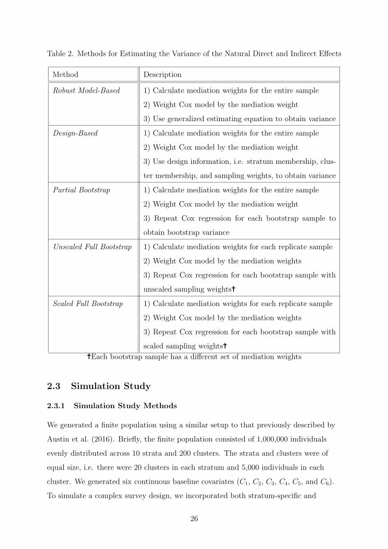
Table 2. Methods for Estimating the Variance of the Natural Direct and Indirect E↵ects
Method Description
Robust Model-Based 1) Calculate mediation weights for the entire sample
2) Weight Cox model by the mediation weight
3) Use generalized estimating equation to obtain variance
Design-Based 1) Calculate mediation weights for the entire sample
2) Weight Cox model by the mediation weight
3) Use design information, i.e. stratum membership, clus-
ter membership, and sampling weights, to obtain variance
Partial Bootstrap 1) Calculate mediation weights for the entire sample
2) Weight Cox model by the mediation weight
3) Repeat Cox regression for each bootstrap sample to
obtain bootstrap variance
Unscaled Full Bootstrap 1) Calculate mediation weights for each replicate sample
2) Weight Cox model by the mediation weights
3) Repeat Cox regression for each bootstrap sample with
unscaled sampling weightsÜ
Scaled Full Bootstrap 1) Calculate mediation weights for each replicate sample
2) Weight Cox model by the mediation weights
3) Repeat Cox regression for each bootstrap sample with
scaled sampling weightsÜÜEach bootstrap sample has a di↵erent set of mediation weights
2.3 Simulation Study
2.3.1 Simulation Study Methods
We generated a finite population using a similar setup to that previously described by
Austin et al. (2016). Briefly, the finite population consisted of 1,000,000 individuals
evenly distributed across 10 strata and 200 clusters. The strata and clusters were of
equal size, i.e. there were 20 clusters in each stratum and 5,000 individuals in each
cluster. We generated six continuous baseline covariates (C1, C2, C3, C4, C5, and C6).
To simulate a complex survey design, we incorporated both stratum-specific and
26
cluster-specific random e↵ects; we defined the random variable for the ith baseline
covariate in the jth stratum and the kth cluster as Cijk ⇠ N(µij + µik, �), where µij and
µik are the stratum-specific e↵ect parameter and the cluster-specific e↵ect parameter,
respectively, i.e. µij ⇠ N(0, ⌧j) and µik ⇠ N(0, ⌧k). Simply put, for each of the six
baseline covariates, we drew two random parameters, which defined the normal
distribution from which the covariates were drawn. We set the standard deviation of
the covariates equal to 1, i.e. � = 1. This setup produced a finite population where
individuals within a given stratum and cluster were more similar than those in di↵erent
strata and clusters, and the proportion of the total variance attributed to di↵erences
between strata and clusters was given by⌧2j
⌧2j
+⌧2k
+1and
⌧2k
⌧2j
+⌧2k
+1, respectively.
We generated a binary exposure, denoted X, by drawing from a Bernouilli distribution
with p = P (X = 1), where P (X = 1) was defined as
log
✓P (X = 1|c)
1� P (X = 1|c)
◆= �0 + �T c. (10)
To be consistent with the work of Austin et al. (2016), we used the following regression
coe�cients to define the binary exposure variable: �0 = log(0.0329/0.9671),
�1 = log(1.1), �2 = log(1.25), �3 = log(1.5), �4 = log(1.75), �5 = log(2), and
�6 = log(2.5). We generated the survival time, denoted T , through a proportional
hazards model with a binary exposure (X), a mediator (M), and a set of baseline
covariates (C). We used the approach developed by Bender et al. (2005), which is
described in detail in appendix A, to simulate the proportional hazards model, i.e.
h(t|x,m, c) = h(t|0, 0, 0)e�0x+�00m+�T c. (11)
We used the following regression coe�cients to define the proportional hazards model:
�0 = 0.5, �00 = log(2.5), �1 = log(1.75), �2 = log(1.75), �3 = �log(1.75),
�4 = �log(1.75), �5 = log(1.25), �6 = �log(1.25). Furthermore, we considered two
distinct setups: one with a rare exposure (3.3% prevalence) and a common outcome
(50% prevalence), and another with a common exposure (50% prevalence) and a rare
outcome (10% prevalence). In the first setup, we used the parameters described above,
and we censored all individuals whose survival time was greater than the 50th percentile
of all survival times. In the second case, we used �0 = 0 instead of
27

�0 = log(0.0329/0.9671), and we censored all individuals whose survival time was
greater than the 10th percentile of all survival times.
We defined the binary mediator through a logistic model, i.e.
log⇣
P (M=1|x,c)1�P (M=1|x,c)
⌘= ↵0 + ↵0x+ ↵T c, and we defined the continuous mediator through a
linear model, i.e. E[M |x, c] = ↵0 + ↵0x+ ↵T c. Then, as shown in appendices B and C,
the natural direct and indirect e↵ects are approximately equal to �0(x� x⇤) and
log
⇣1+e↵0+↵
0x
⇤+↵
T
c
⌘⇣1+e↵0+↵
0x+↵
T
c+�
00⌘
(1+e↵0+↵
0x+↵
T
c)(1+e↵0+↵
0x
⇤+↵
T
c+�
00)
�for the binary mediator and �0(x� x⇤) and
�00↵0(x� x⇤) for the continuous mediator. For the binary mediator, we used the
following regression coe�cients: ↵0 = 0, ↵0 = log(2.5), ↵1 = log(1.25), ↵2 = �log(1.25),
↵3 = log(1.25), ↵4 = �log(1.25), ↵5 = log(1.75), and ↵6 = �log(1.75). It is important
to note that when the mediator is binary, the natural indirect e↵ect depends on the
level of the baseline covariates. In other words, it is possible to calculate the natural
indirect e↵ect for di↵erent levels of the baseline covariates (e.g. C1 = 0 vs. C1 = 1). To
obtain the average natural indirect e↵ect, we set each baseline covariate equal to its
average value. For the continuous mediator, we used the following regression
coe�cients: ↵0 = 0, ↵0 = 0.25, ↵1 = log(1.25), ↵2 = �log(1.25), ↵3 = log(1.25),
↵4 = �log(1.25), ↵5 = log(1.75), and ↵6 = �log(1.75). Finally, we used a standard
deviation of 0.5 to define the linear mediation model.
To obtain our samples, we drew 5,000 individuals from the finite population. We
randomly assigned one of the following sample sizes to each of the 10 strata: 250, 300,
350, 400, 450, 550, 600, 650, 700, 750. We selected 5 clusters from each stratum using
SRS, and then we sampled an equal number of individuals from within each of the 5
clusters using SRS. Next, we calculated the sampling weight for each individual, which
is simply the inverse of the selection probability. If n individuals were selected from a
stratum of size N , then the selection probability for each of the n individuals was
obtained by taking the product of the probability of selecting a cluster and the
probability of selecting an individual from within the cluster, i.e. ⇡ = ⇡Clu ⇥ ⇡Ind|Clus.
Since 5 out of 20 clusters were selected within each stratum, and since n/5 individuals
were selected from within each cluster, the probability of selecting a cluster and the
probability of selecting an individual from within the given cluster were ⇡Clu = 520 and
⇡Ind|Clus =n/5N/20 , respectively. Thus, the selection probability was given by
28
⇡ = ⇡Clu ⇥ ⇡Ind|Clus =nN, and the sampling weight was equal to w = 1
⇡= N
n. We created
500 bootstrap weights by re-sampling clusters from each stratum. To be consistent with
the sampling design of the CCHS, which re-samples n� 1 out of n clusters with
replacement from each stratum (Statistics Canada, 2002), we re-sampled 4 clusters with
replacement from each stratum and re-weighted the bootstrap samples accordingly.
We simulated 1,000 samples by making repeated draws from the finite population using
the aforementioned sampling scheme. We then applied the methods described in
Section 2.2. For each sample, we obtained multiple di↵erent estimates for both the
natural direct and indirect e↵ects (and their corresponding variances). We combined
this information to construct approximate 95% confidence intervals, i.e.
✓i ± 1.96⇥q
�2(✓i), where ✓ and �2(✓) denote the point estimate and the variance
estimate, respectively, in the ith sample. The bias was defined as
BIAS = 11,000
P1,000i=1 (✓i � ✓), where ✓ is the parameter of interest in the finite
population. The percentage bias was defined as 100⇥ BIAS✓
. The MSE was defined as
MSE = 11,000
P1,000i=1 (✓i � ✓)2, while the relative MSE was defined as MSE
✓2. Finally,
coverage of the 95% confidence interval was calculated as the proportion of confidence
intervals that included the point estimate from the finite population. We created six
di↵erent simulation setups by varying the value of ⌧j and ⌧k, which are the
stratum-specific and cluster-specific random e↵ects parameters, respectively. We did
this in order to assess the impact of between-cluster and between-stratum variation, and
also to identify general trends across all settings. In the first three settings, we used
⌧k = 0.35 and ⌧j = 0.25, 0.15, 0.05; in the latter three settings, we used ⌧j = 0.35 and
⌧k = 0.25, 0.15, 0.05. After specifying these parameters, we determined the proportion of
the total variance attributed to di↵erences between strata and clusters.
All analyses were performed using R statistical programming language version 3.3.3 (R
Core Team, 2017). The unweighted linear models, the frequency weighted linear
models, and the unweighted logistic models were fitted using the glm function in the
stats package; the sample weighted linear models were fitted using the svyglm function
in the survey package; the weighted logistic models were fitted using the vglm function
in the VGAM package; the unweighted Cox models were fitted using the coxph function
in the survival package; the sample weighted Cox models were fitted using the svycoxph
29

function in the survey package.
2.3.2 Simulation Study Results
We first considered the setup with a rare exposure (3.3% prevalence) and a common
outcome (50% prevalence). The percentage bias for the binary and continuous
mediators are presented in Figures 1 and 2. None of the methods were universally best
at reducing bias. In the case of the binary mediator, each of the four methods had the
smallest percentage bias in at least one of the six settings. We obtained nearly identical
results with the continuous mediator, with the only exception being the unscaled
weighted method, which consistently produced estimates with the largest bias (see
Figure 5). In each setting, we compared the percentage bias of the unscaled weighted
method to the estimate with the second largest percentage bias. The magnitude of the
percentage bias obtained with the unscaled weighted method was 28 to 377 times
greater than the second worst estimate in each setting. The relative MSEs are shown in
Figures 3 and 4. The unweighted and covariate methods generally produced the
smallest relative MSE. The relative MSEs for the sample weighted and hybrid methods
were similar for the natural direct e↵ect, but the relative MSE for the sample weighted
method was consistently larger than that of the hybrid method for the natural indirect
e↵ect. Finally, in the case of the continuous mediator, the unscaled weighted method
always produced estimates with the largest relative MSE (see Figure 5). Similar to our
analysis of the percentage bias, we compared the relative MSE of the unscaled weighted
method to the estimate with the second largest MSE in each setting. The relative MSE
obtained with the unscaled weighted method was 5 to 61 times greater than the second
worst estimate in each setting. We obtained nearly identical results for the setup with a
common exposure (50% prevalence) and a rare outcome (10% censoring), as shown in
appendices F and G.
30

●
Stratum: 5.3%, Cluster: 10.3%Pe
rcen
tage
Bia
s
● ● ● ●
Unweighted Covariate ScaledWeighted
Hybrid
−3.0
0.0
1.5
3.0
●
Stratum: 2.0%, Cluster: 10.3%
Perc
enta
ge B
ias
● ●● ●
Unweighted Covariate ScaledWeighted
Hybrid
−3.0
0.0
1.5
3.0
Stratum: 0.2%, Cluster: 10.3%
Perc
enta
ge B
ias
● ●● ●
Unweighted Covariate ScaledWeighted
Hybrid
−3.0
0.0
1.5
3.0
●
Stratum: 10.3%, Cluster: 5.3%
Perc
enta
ge B
ias
● ● ● ●
Unweighted Covariate ScaledWeighted
Hybrid
−3.0
0.0
1.5
3.0
●
Stratum: 10.3%, Cluster: 2.0%
Perc
enta
ge B
ias
● ●● ●
Unweighted Covariate ScaledWeighted
Hybrid
−3.0
0.0
1.5
3.0
Stratum: 10.3%, Cluster: 0.2%
Perc
enta
ge B
ias
● ● ● ●
Unweighted Covariate ScaledWeighted
Hybrid
−3.0
0.0
1.5
3.0
● Natural Direct Effect Natural Indirect Effect
Figure 1. Percentage bias from the simulations with a binary mediator, a rare binary
exposure (3.3% prevalence), and a common outcome (50% prevalence). We considered six
di↵erent settings (by varying the proportion of the total variance attributed to di↵erences
between strata and clusters), and we implemented all methods outlined in section 2.2.
Percentage bias was defined as 11,000
P1,000i=1
⇣✓i
�✓✓
⌘, where ✓ is the parameter of interest in
the finite population.
31

●
Stratum: 5.3%, Cluster: 10.3%Pe
rcen
tage
Bia
s
● ● ● ●
●
Unweighted Covariate ScaledWeighted
Hybrid UnscaledWeighted
−100
−50
050
100
Stratum: 2.0%, Cluster: 10.3%
Perc
enta
ge B
ias
● ● ● ●
●
Unweighted Covariate ScaledWeighted
Hybrid UnscaledWeighted
−100
−50
050
100
Stratum: 0.2%, Cluster: 10.3%
Perc
enta
ge B
ias
● ● ● ●
●
Unweighted Covariate ScaledWeighted
Hybrid UnscaledWeighted
−100
−50
050
100
●
Stratum: 10.3%, Cluster: 5.3%
Perc
enta
ge B
ias
● ● ● ●
●
Unweighted Covariate ScaledWeighted
Hybrid UnscaledWeighted
−100
−50
050
100
Stratum: 10.3%, Cluster: 2.0%
Perc
enta
ge B
ias
● ● ● ●
●
Unweighted Covariate ScaledWeighted
Hybrid UnscaledWeighted
−100
−50
050
100
Stratum: 10.3%, Cluster: 0.2%
Perc
enta
ge B
ias
● ● ● ●
●
Unweighted Covariate ScaledWeighted
Hybrid UnscaledWeighted
−100
−50
050
100
● Natural Direct Effect Natural Indirect Effect
Figure 2. Percentage bias from the simulations with a continuous mediator, a rare binary
exposure (3.3% prevalence), and a common outcome (50% prevalence). We considered six
di↵erent settings (by varying the proportion of the total variance attributed to di↵erences
between strata and clusters), and we implemented all methods outlined in section 2.2.
Percentage bias was defined as 11,000
P1,000i=1
⇣✓i
�✓✓
⌘, where ✓ is the parameter of interest in
the finite population.
32
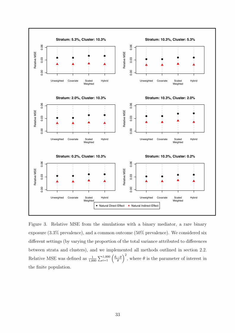
Stratum: 5.3%, Cluster: 10.3%R
elat
ive M
SE
● ●● ●
Unweighted Covariate ScaledWeighted
Hybrid
0.00
0.03
0.06
Stratum: 2.0%, Cluster: 10.3%
Rel
ative
MSE
● ●● ●
Unweighted Covariate ScaledWeighted
Hybrid
0.00
0.03
0.06
Stratum: 0.2%, Cluster: 10.3%
Rel
ative
MSE
● ●● ●
Unweighted Covariate ScaledWeighted
Hybrid
0.00
0.03
0.06
Stratum: 10.3%, Cluster: 5.3%
Rel
ative
MSE
● ●● ●
Unweighted Covariate ScaledWeighted
Hybrid
0.00
0.03
0.06
Stratum: 10.3%, Cluster: 2.0%
Rel
ative
MSE
● ●● ●
Unweighted Covariate ScaledWeighted
Hybrid
0.00
0.03
0.06
Stratum: 10.3%, Cluster: 0.2%
Rel
ative
MSE
● ●● ●
Unweighted Covariate ScaledWeighted
Hybrid
0.00
0.03
0.06
● Natural Direct Effect Natural Indirect Effect
Figure 3. Relative MSE from the simulations with a binary mediator, a rare binary
exposure (3.3% prevalence), and a common outcome (50% prevalence). We considered six
di↵erent settings (by varying the proportion of the total variance attributed to di↵erences
between strata and clusters), and we implemented all methods outlined in section 2.2.
Relative MSE was defined as 11,000
P1,000i=1
⇣✓i
�✓✓
⌘2, where ✓ is the parameter of interest in
the finite population.
33

Stratum: 5.3%, Cluster: 10.3%R
elat
ive M
SE
● ● ● ●
Unweighted Covariate ScaledWeighted
Hybrid
0.00
0.03
0.06
Stratum: 2.0%, Cluster: 10.3%
Rel
ative
MSE
● ●● ●
Unweighted Covariate ScaledWeighted
Hybrid
0.00
0.03
0.06
Stratum: 0.2%, Cluster: 10.3%
Rel
ative
MSE
● ●● ●
Unweighted Covariate ScaledWeighted
Hybrid
0.00
0.03
0.06
Stratum: 10.3%, Cluster: 5.3%
Rel
ative
MSE
● ●● ●
Unweighted Covariate ScaledWeighted
Hybrid
0.00
0.03
0.06
Stratum: 10.3%, Cluster: 2.0%
Rel
ative
MSE
● ●● ●
Unweighted Covariate ScaledWeighted
Hybrid
0.00
0.03
0.06
Stratum: 10.3%, Cluster: 0.2%
Rel
ative
MSE
● ●● ●
Unweighted Covariate ScaledWeighted
Hybrid
0.00
0.03
0.06
● Natural Direct Effect Natural Indirect Effect
Figure 4. Relative MSE from the simulations with a continuous mediator, a rare binary
exposure (3.3% prevalence), and a common outcome (50% prevalence). We considered six
di↵erent settings (by varying the proportion of the total variance attributed to di↵erences
between strata and clusters), and we implemented all methods outlined in section 2.2.
Relative MSE was defined as 11,000
P1,000i=1
⇣✓i
�✓✓
⌘2, where ✓ is the parameter of interest in
the finite population.
34

●
Perc
enta
ge B
ias
● ● ● ●
●
Unweighted Covariate Weighted Hybrid Frequency
−100
010
0
Rel
ative
MSE
● ● ● ●
●
Unweighted Covariate Weighted Hybrid Frequency
0.00
0.15
0.30
● Natural Direct Effect Natural Indirect Effect
Figure 5. Complete percentage bias and relative MSE for the first setting from the
simulations with a continuous mediator, a rare binary exposure (3.3% prevalence), and a
common outcome (50% prevalence).
Coverage rates of the 95% confidence interval for both the natural direct and indirect
e↵ects obtained from the simulations with a rare exposure (3.3% prevalence) and a
common outcome (50% censoring) are presented in Tables 3 and 4. Since the findings
are nearly identical in all six settings, we present results from the first setting in the
main body of this report and refer the reader to appendices D and E for complete
results. All variance estimators produced appropriate coverage of the 95% confidence
35
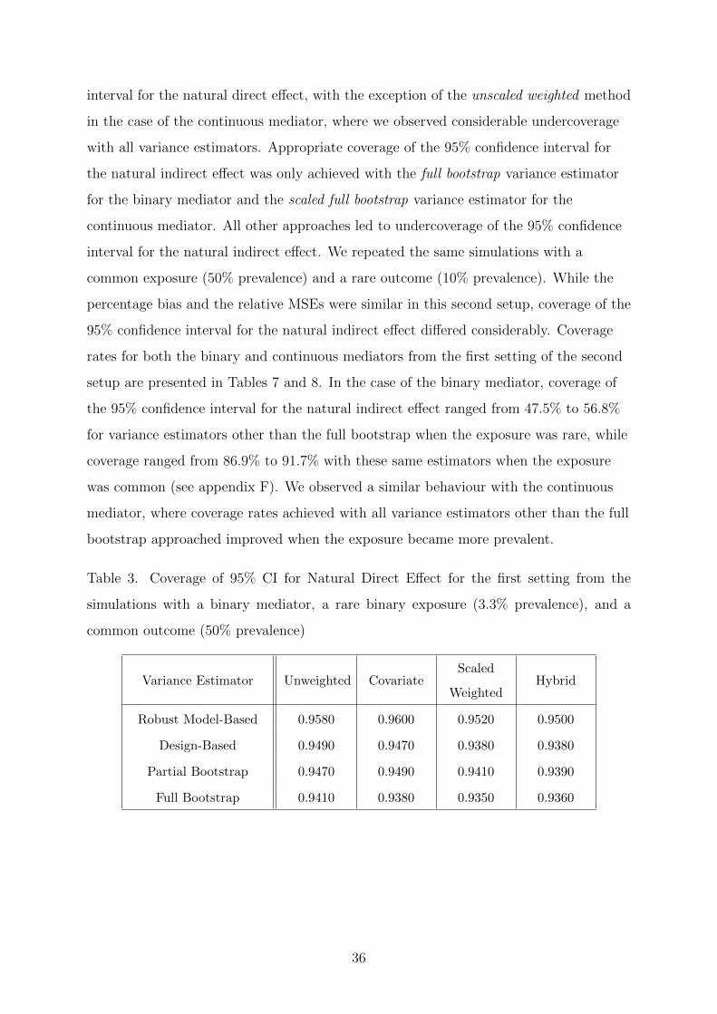
interval for the natural direct e↵ect, with the exception of the unscaled weighted method
in the case of the continuous mediator, where we observed considerable undercoverage
with all variance estimators. Appropriate coverage of the 95% confidence interval for
the natural indirect e↵ect was only achieved with the full bootstrap variance estimator
for the binary mediator and the scaled full bootstrap variance estimator for the
continuous mediator. All other approaches led to undercoverage of the 95% confidence
interval for the natural indirect e↵ect. We repeated the same simulations with a
common exposure (50% prevalence) and a rare outcome (10% prevalence). While the
percentage bias and the relative MSEs were similar in this second setup, coverage of the
95% confidence interval for the natural indirect e↵ect di↵ered considerably. Coverage
rates for both the binary and continuous mediators from the first setting of the second
setup are presented in Tables 7 and 8. In the case of the binary mediator, coverage of
the 95% confidence interval for the natural indirect e↵ect ranged from 47.5% to 56.8%
for variance estimators other than the full bootstrap when the exposure was rare, while
coverage ranged from 86.9% to 91.7% with these same estimators when the exposure
was common (see appendix F). We observed a similar behaviour with the continuous
mediator, where coverage rates achieved with all variance estimators other than the full
bootstrap approached improved when the exposure became more prevalent.
Table 3. Coverage of 95% CI for Natural Direct E↵ect for the first setting from the
simulations with a binary mediator, a rare binary exposure (3.3% prevalence), and a
common outcome (50% prevalence)
Variance Estimator Unweighted CovariateScaled
WeightedHybrid
Robust Model-Based 0.9580 0.9600 0.9520 0.9500
Design-Based 0.9490 0.9470 0.9380 0.9380
Partial Bootstrap 0.9470 0.9490 0.9410 0.9390
Full Bootstrap 0.9410 0.9380 0.9350 0.9360
36

Table 4. Coverage of 95% CI for Natural Indirect E↵ect for the first setting from the
simulations with a binary mediator, a rare binary exposure (3.3% prevalence), and a
common outcome (50% prevalence)
Variance Estimator Unweighted CovariateScaled
WeightedHybrid
Robust Model-Based 0.5210 0.5200 0.5160 0.5500
Design-Based 0.5230 0.5240 0.5070 0.5450
Partial Bootstrap 0.5230 0.5250 0.5140 0.5400
Full Bootstrap 0.9390 0.9420 0.9440 0.9440
Table 5. Coverage of 95% CI for Natural Direct E↵ect for the first setting from the
simulations with a continuous mediator, a rare binary exposure (3.3% prevalence), and a
common outcome (50% prevalence)
Variance Estimator Unweighted CovariateScaled
WeightedHybrid
Unscaled
Weighted
Robust Model-Based 0.9460 0.9460 0.9520 0.9480 0.3160
Design-Based 0.9340 0.9340 0.9390 0.9390 0.3150
Partial Bootstrap 0.9350 0.9380 0.9440 0.9420 0.3300
Unscaled Full Bootstrap 0.9230 0.9250 – 0.9270 0.3290
Scaled Full Bootstrap 0.9270 0.9260 0.9340 0.9340 –
Table 6. Coverage of 95% CI for Natural Indirect E↵ect for the first setting from the
simulations with a continuous mediator, a rare binary exposure (3.3% prevalence), and a
common outcome (50% prevalence)
Variance Estimator Unweighted CovariateScaled
WeightedHybrid
Unscaled
Weighted
Robust Model-Based 0.5450 0.5450 0.5470 0.5630 0.0000
Design-Based 0.5310 0.5290 0.5340 0.5460 0.0000
Partial Bootstrap 0.5330 0.5310 0.5370 0.5540 0.0000
Unscaled Full Bootstrap 0.7990 0.7990 – 0.8040 0.0000
Scaled Full Bootstrap 0.9230 0.9240 0.9360 0.9210 –
37

Table 7. Coverage of 95% CI for Natural Direct E↵ect for the first setting from the
simulations with a binary mediator, a common exposure (50% prevalence), and a rare
outcome (10% prevalence)
Variance Estimator Unweighted CovariateScaled
WeightedHybrid
Robust Model-Based 0.9440 0.9440 0.9430 0.9410
Design-Based 0.9350 0.9340 0.9320 0.9330
Partial Bootstrap 0.9410 0.9390 0.9350 0.9350
Full Bootstrap 0.9400 0.9390 0.9360 0.9340
Table 8. Coverage of 95% CI for Natural Indirect E↵ect for the first setting from the
simulations with a binary mediator, a common exposure (50% prevalence), and a rare
outcome (10% prevalence)
Variance Estimator Unweighted CovariateScaled
WeightedHybrid
Robust Model-Based 0.8800 0.8800 0.8710 0.8880
Design-Based 0.8870 0.8850 0.8700 0.8840
Partial Bootstrap 0.8850 0.8860 0.8690 0.8830
Full Bootstrap 0.9400 0.9400 0.9250 0.9330
Table 9. Coverage of 95% CI for Natural Direct E↵ect for the first setting from the
simulations with a continuous mediator, a common exposure (50% prevalence), and a
rare outcome (10% prevalence)
Variance Estimator Unweighted CovariateScaled
WeightedHybrid
Unscaled
Weighted
Robust Model-Based 0.9570 0.9570 0.9610 0.9620 0.5170
Design-Based 0.9520 0.9550 0.9540 0.9520 0.5140
Partial Bootstrap 0.9530 0.9530 0.9530 0.9570 0.5200
Unscaled Full Bootstrap 0.9470 0.9480 – 0.9470 0.5200
Scaled Full Bootstrap 0.9500 0.9500 0.9530 0.9530 –
38
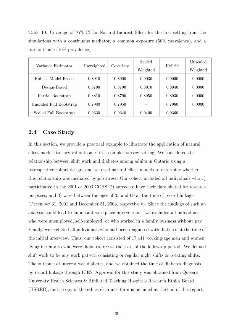
Table 10. Coverage of 95% CI for Natural Indirect E↵ect for the first setting from the
simulations with a continuous mediator, a common exposure (50% prevalence), and a
rare outcome (10% prevalence)
Variance Estimator Unweighted CovariateScaled
WeightedHybrid
Unscaled
Weighted
Robust Model-Based 0.8910 0.8900 0.9030 0.9060 0.0000
Design-Based 0.8790 0.8790 0.8910 0.8940 0.0000
Partial Bootstrap 0.8810 0.8790 0.8950 0.8930 0.0000
Unscaled Full Bootstrap 0.7980 0.7950 – 0.7960 0.0000
Scaled Full Bootstrap 0.9330 0.9340 0.9400 0.9360 –
2.4 Case Study
In this section, we provide a practical example to illustrate the application of natural
e↵ect models to survival outcomes in a complex survey setting. We considered the
relationship between shift work and diabetes among adults in Ontario using a
retrospective cohort design, and we used natural e↵ect models to determine whether
this relationship was mediated by job stress. Our cohort included all individuals who 1)
participated in the 2001 or 2003 CCHS, 2) agreed to have their data shared for research
purposes, and 3) were between the ages of 35 and 69 at the time of record linkage
(December 31, 2001 and December 31, 2003, respectively). Since the findings of such an
analysis could lead to important workplace interventions, we excluded all individuals
who were unemployed, self-employed, or who worked in a family business without pay.
Finally, we excluded all individuals who had been diagnosed with diabetes at the time of
the initial interview. Thus, our cohort consisted of 17,441 working-age men and women
living in Ontario who were diabetes-free at the start of the follow-up period. We defined
shift work to be any work pattern consisting or regular night shifts or rotating shifts.
The outcome of interest was diabetes, and we obtained the time of diabetes diagnosis
by record linkage through ICES. Approval for this study was obtained from Queen’s
University Health Sciences & A�liated Teaching Hospitals Research Ethics Board
(HSREB), and a copy of the ethics clearance form is included at the end of this report.
39

To measure job stress, the CCHS includes 12 questions related to various di↵erent
psychosocial job characteristics. The interviewer reads a statement about a specific job
characteristic, and the participants are asked to indicate how strongly they agree with
the given statement. For example, the first statement reads, “Please tell me if you
strongly agree, agree, neither agree nor disagree, disagree, or strongly disagree. Your
job required that you learn new things” (Statistics Canada, 2003a). The answers are
scored on a scale from 1 (strongly disagree) to 5 (strongly agree), and the questions are
combined to produce the following six measures, which are derived from the Job
Content Questionnaire (Karasek et al., 1998): 1) skill discretion, 2) decision authority,
3) psychological demands, 4) job insecurity, 5) physical exertion, and 6) social support.
The composite variables are scored using scales from 0 to 4, 0 to 8, or 0 to 12, and these
variables are then combined to produce an overall measure of job stress with values
ranging from 0 to 48 (Statistics Canada, 2003b). To be consistent with Smith et al.
(2012), who examined the relationship between job stress and the incidence of diabetes
among adults in Ontario, we did not include job insecurity or physical exertion in our
definition of job stress. In other words, we only considered skill discretion, decision
authority, psychological demands, and social support; we combined these four variables
to obtain an overall measure of job stress. Decision latitude (skill discretion) and social
support are measured on a scale from 0 to 12, while decision latitude (decision
authority) and psychological demands are given in terms of an 8-point scale. Thus, the
overall measure of job stress can be treated as a continuous variable with values ranging
from 0 to 40.
To be consistent with the literature, we treated the following variables as confounders:
age, sex, education, ethnicity, marital status, BMI, physical activity, smoking status,
alcohol consumption. A systematic review published in 2014 identified six cohort
studies that considered the relationship between shift work and diabetes (Knutsson
et al., 2014). According to this systematic review, the most important confounders are
age, BMI, family history of diabetes, smoking status, and physical activity (Knutsson
et al., 2014). All of the studies identified in this systematic review included either only
males or only females. Since our dataset included both men and women, we also
adjusted for sex. Finally, in addition to the most important confounders suggested by
Knutsson et al. (2014), we also considered education, ethnicity, marital status, and
40

alcohol consumption as potential confounders. All of these additional variables were
included in at least one of the studies included in the systematic review (Knutsson
et al., 2014), and we believed that it was possible for each one of these variable to be
causally associated with both shift work and diabetes diagnosis.
We used natural e↵ect models (as described in Section 2.2) to determine whether job
stress was a mediator of the relationship between shift work and diabetes diagnosis in
our cohort. In order to satisfy the assumptions of natural e↵ect models (Lange et al.,
2012), we included confounders of the exposure-mediator and mediator-outcome
relationships. In other words, we considered all confounders of the following
relationships: 1) shift work and job stress (Knutsson and Nilsson, 1997; Bøggild et al.,
2001), and 2) job stress and diabetes Smith et al. (2012). The complete list of
confounders is presented in a causal diagram in Figure 6. We defined the mediator
variable to be the total measure of job stress, which was given in terms of a scale from 0
to 40. We performed two separate mediation analyses, treating job stress as a binary
variable in the first and as a continuous variable in the second. We defined the binary
mediator by using the population median of the total measure of job stress as the
binary cut-point; in other words, all individuals who reported having a total job stress
greater than the population median were considered to be exposed, while all other
individuals were considered to be unexposed. To obtain the populaton median, we used
the svyquantile function, which uses sampling weights to compute the quantiles in the
population from which the sample is drawn (Lumley, 2010).
41

Figure 6. Causal diagram of the relationship between shift work, job stress, and diabetes.
We considered all methods outlined in Section 2.2 that could be implemented with the
design information provided with the CCHS dataset. We obtained point estimates for
both the binary and continuous mediator using the following methods: unweighted,
covariate, sample weighted, and hybrid. In the case of the continuous mediator, we also
implemented the unscaled weighted method. While we were able to obtain point
estimates for all of these approaches, we could only implement a limited number of
variance estimators. Statistics Canada does not release stratum and cluster membership
information for the CCHS, which means that we could not use the design-based
variance estimator. Bootstrap samples are created by re-sampling clusters from within
each stratum with replacement. Thus, stratum and cluster membership must be known
in order to use the partial bootstrap and full bootstrap variance estimators generally.
Statistics Canada creates a set of 500 replicate weights, which are obtained by first
creating bootstrap samples by re-sampling n� 1 clusters from within each stratum with
replacement. Each bootstrap sample is then multiplied by the sampling weight and
42

post-stratified separately. Since the bootstrap samples are embedded in the replicate
weights, the partial bootstrap and full bootstrap variance estimators can only be
implemented with the scaled weighted and unscaled weighted methods. In our analysis,
we found that none of the methods produced statistically significant estimates of either
the natural direct e↵ect or the natural indirect e↵ect. Complete estimates of the natural
direct and indirect e↵ects for both the binary and continuous mediators are presented in
Tables 11 to 14.
Table 11. 95% CI of Natural Direct E↵ect (Job Stress as a Binary Variable)
Method Unweighted CovariateScaled
WeightedHybrid
Point Estimate -0.007 -0.004 -0.053 -0.049
Robust Model-Based (-0.17,0.15) (-0.17,0.16) (-0.28,0.17) (-0.28,0.18)
Design-Based – – – –
Partial Bootstrap – – (-0.28,0.17) (-0.28,0.18)
Full Bootstrap – – (-0.28,0.17) –
n = 9, 601 (excluded 7,840 individuals with missing data)
Table 12. 95% CI of Natural Indirect E↵ect (Job Stress as a Binary Variable)
Method Unweighted CovariateScaled
WeightedHybrid
Point Estimate 0.001 0.002 0.005 0.004
Robust Model-Based (-0.02,0.02) (-0.02,0.02) (-0.02,0.03) (-0.02,0.03)
Design-Based – – – –
Partial Bootstrap – – (-0.02,0.03) (-0.02,0.03)
Full Bootstrap – – (-0.02,0.03) –
n = 9, 601 (excluded 7,840 individuals with missing data)
43
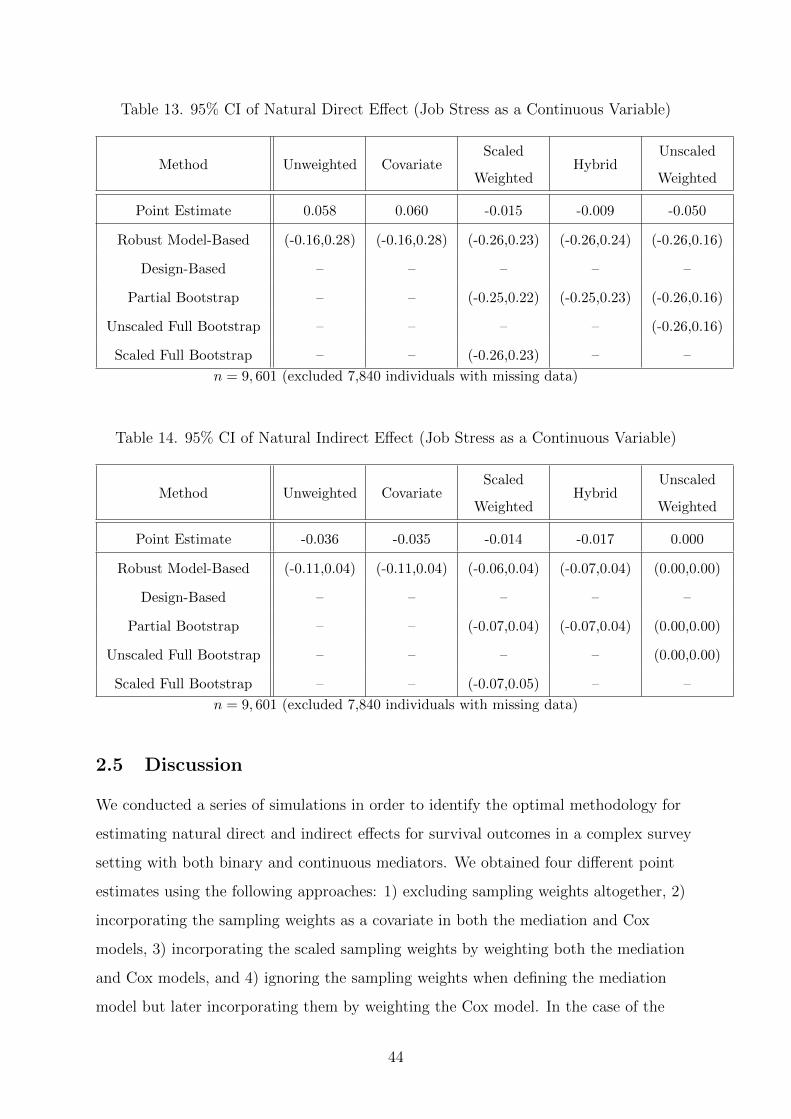
Table 13. 95% CI of Natural Direct E↵ect (Job Stress as a Continuous Variable)
Method Unweighted CovariateScaled
WeightedHybrid
Unscaled
Weighted
Point Estimate 0.058 0.060 -0.015 -0.009 -0.050
Robust Model-Based (-0.16,0.28) (-0.16,0.28) (-0.26,0.23) (-0.26,0.24) (-0.26,0.16)
Design-Based – – – – –
Partial Bootstrap – – (-0.25,0.22) (-0.25,0.23) (-0.26,0.16)
Unscaled Full Bootstrap – – – – (-0.26,0.16)
Scaled Full Bootstrap – – (-0.26,0.23) – –
n = 9, 601 (excluded 7,840 individuals with missing data)
Table 14. 95% CI of Natural Indirect E↵ect (Job Stress as a Continuous Variable)
Method Unweighted CovariateScaled
WeightedHybrid
Unscaled
Weighted
Point Estimate -0.036 -0.035 -0.014 -0.017 0.000
Robust Model-Based (-0.11,0.04) (-0.11,0.04) (-0.06,0.04) (-0.07,0.04) (0.00,0.00)
Design-Based – – – – –
Partial Bootstrap – – (-0.07,0.04) (-0.07,0.04) (0.00,0.00)
Unscaled Full Bootstrap – – – – (0.00,0.00)
Scaled Full Bootstrap – – (-0.07,0.05) – –
n = 9, 601 (excluded 7,840 individuals with missing data)
2.5 Discussion
We conducted a series of simulations in order to identify the optimal methodology for
estimating natural direct and indirect e↵ects for survival outcomes in a complex survey
setting with both binary and continuous mediators. We obtained four di↵erent point
estimates using the following approaches: 1) excluding sampling weights altogether, 2)
incorporating the sampling weights as a covariate in both the mediation and Cox
models, 3) incorporating the scaled sampling weights by weighting both the mediation
and Cox models, and 4) ignoring the sampling weights when defining the mediation
model but later incorporating them by weighting the Cox model. In the case of the
44

continuous mediator, we also considered unscaled sampling weights to obtain a fifth
estimate. We assessed the performance of each method by comparing percentage bias,
relative MSE, and coverage rates of the 95% confidence interval.
Based on the results of our simulations, we conclude that none of the methods are
universally best. For the binary mediator, we obtained similar percentage bias for both
the natural direct and indirect e↵ects using all four methods. However, we noted a
di↵erence in terms of relative MSE; the methods that did not weight the Cox model by
the sampling weights were consistently better than their weighted counterparts. We
observed nearly identical results with a continuous mediator. We also implemented an
additional method that was not considered for the binary mediator. When we used
unscaled sampling weights, which is analogous to specifying frequency weights instead
of sampling weights, the percentage bias and the relative MSE increased drastically.
While misspecifying the type of weight in a regression model will not a↵ect the point
estimates of the regression coe�cients, it will lead to incorrect variance estimates. In
our simulations, we noticed that the residual variance was much greater when we
treated the sampling weights as frequency weights. Interestingly, the natural indirect
e↵ect converged to 0 in this situation. These findings highlight the importance of
correctly specifying the sampling weights when using natural e↵ect models with a
continuous mediator. In other words, the sampling weights should always be multiplied
by a scaling factor such that their sum is equal to the number of observations in the
dataset. Thus, if a dataset contains n observations, the mediation weights should be
divided by the sum of the weights and then multiplied by n.
We also compared the performance of di↵erent variance estimators. First, we used the
robust model-based variance estimator suggested by Lange et al. (2012). We compared
this estimator to a fully design-based variance estimator and to two types of bootstrap
variance estimators. The first bootstrap approach consisted of repeating only the Cox
model (i.e. same mediation weights for all bootstrap samples), while the second was
obtained by re-defining the mediation model for each bootstrap sample (i.e. di↵erent set
of mediation weights for each bootstrap sample). For the binary mediator, we obtained
appropriate coverage of the 95% confidence interval for the natural direct e↵ect with all
methods and variance estimators. However, appropriate coverage of the 95% confidence
45

interval for the natural indirect e↵ect was only achieved when we re-defined the
mediation model for each bootstrap sample; all other variance estimators led to
undercoverage. We observed similar results with the continuous mediator, where all
variance estimators produced undercoverage of the 95% confidence interval for the
natural indirect e↵ect, with the exception of the situation where we re-defined the
mediation model for each setting. For the continuous mediator, we implemented this
technique in two di↵erent ways. First, we used the weights of the original sample and,
second, we re-scaled the weights such that their sum was equal to the number of unique
observations in the bootstrap sample. The latter approach produced appropriate
coverage rates, while the former approach did not. Furthermore, when we treated the
sampling weights as frequency weights, we obtained very poor coverage of the 95%
confidence interval for both the natural direct and indirect e↵ects, which is mostly due
to the bias described in the preceding paragraph. Thus, we conclude that it is
important to perform a full bootstrap in order to obtain appropriate variance estimates
of the natural indirect e↵ect (for both binary and continuous mediators). In other
words, the mediation model should be re-defined for each bootstrap sample. Finally,
with a continuous mediator, the bootstrap weights should be re-scaled to the number of
unique observations in the bootstrap sample.
We performed simulations using two distinct setups. First, we considered a rare
exposure (3.3% prevalence) with a common outcome (50% prevalence) and, second, we
considered a common exposure (50% prevalence) with a rare outcome (10% prevalence).
Both of these setups resulted in undercoverage of the 95% confidence interval for the
natural indirect e↵ect when a full bootstrap approach was not employed. However,
coverage rates improved when we increased the prevalence of the exposure (see
appendices F and G). The only exception to this occurred when we treated the
sampling weights as frequency weights, where coverage rates were 0.0% in all settings
for both setups. The fact that coverage of the natural indirect e↵ect improves as the
prevalence of the exposure increases can be explained as follows. The mediation model
is obtained by regressing the mediator against the exposure and baseline covariates.
The variance of a binary covariate in both linear and logistic models is minimized when
the covariate has a prevalence of 50%, as shown in appendix H. As a result, the
mediation weights become more variable when the exposure becomes increasingly rare.
46

The variance estimators that produce undercoverage all employ a single set of
mediation weights based on the full sample, which means that they do not account for
this source of variability. Thus, all methods other than the approach that re-defines the
mediation model for each bootstrap sample underestimate the true variance, and the
discrepancy between these estimates and the true variance becomes more pronounced
when the exposure is rare.
In the last section of this report, we considered a practical example to illustrate the
application of natural e↵ect models to survival outcomes in a complex survey setting.
Through this example, we showed that only one of the proper variance estimators could
be implemented with both binary and continuous mediators. This is due to the fact
that Statistics Canada does not release design information, which is necessary to create
bootstrap samples. Instead, the CCHS dataset includes 500 replicate weights, which are
each post-stratified separately. As a result, all design information is embedded in the
replicate weights, and a full bootstrap can only be achieved if both the mediation model
and the Cox model are weighted by the replicate weights. Thus, we conclude that
analysts wishing to implement natural e↵ect models with data from complex surveys
should perform a full bootstrap with weighted mediation and Cox models if they are
provided with replicate weights but not design information. However, we note that the
full bootstrap variance estimator performs equally well when the Cox model is not
weighted by the sampling weights. In fact, in our simulations, the MSE was slightly
smaller when the Cox model was not weighted by the sampling weights. Thus, it may
be preferable to use one of the unweighted methods if appropriate bootstrap samples
can be created from the available design information.
47

A Simulating Proportional Hazards Model
Linear models can be simulated by specifying the desired regression coe�cients and
drawing a random error term for each data point (Bender et al., 2005). The simplicity
of this approach is due to the fact that the variables and the regression coe�cients are
defined on the same scale (i.e. in a simple linear model, a one unit increase of the
independent variable leads to a change of the dependent variable by a factor equal to
the regression coe�cient). Advanced methodology must be employed to create
simulated models when the relationship between variables and regression coe�cients is
more elaborate (Bender et al., 2005). This is especially true for proportional hazards
models, where the regression coe�cients are defined on the hazard scale, while the
dependent variable is given as a unit of time (Kleinbaum and Klein, 2011). In addition
to the challenge of reconciling these quantities, proportional hazards models must also
be simulated in a way that ensures that the proportional hazards assumption is
satisfied. Fully parametric models that satisfy the proportional hazards assumption,
such as the exponential, Weibull, and Gompertz distributions, can be employed (Bender
et al., 2005). However, it is not obvious how the parameters of the fully parametric
distributions relate to those in a proportional hazards model. In other words, it is easy
to generate survival times that satisfy the proportional hazards assumption, but it can
be di�cult to determine the value of the expected regression coe�cients in the
corresponding proportional hazards model. Bender et al. (2005) developed a technique
to simulate proportional hazards models with pre-determined parameters by using
exponential, Weibull, and Gompertz distributions. Since the exponential and Weibull
distributions satisfy both the proportional hazards assumption and the AFT
assumption, they are more general than the Gompertz distribution, which violates the
AFT assumption (Kleinbaum and Klein, 2011). Furthermore, the exponential
distribution is special case of the Weibull distribution that assumes a constant hazard
(Kleinbaum and Klein, 2011). Due to this strong restriction, we chose to use the
Weibull distribution to simulate survival times.
The density function of the Weibull distribution is defined for ⇢ > 0 and � > 0 as
f(t|�, ⇢) = ⇢�t⇢�1e��t⇢ . (12)
48

Note that ⇢ is said to be the shape parameter, while � is said to the be the scale
parameter. The Weibull distribution reduces to the exponential distribution when ⇢ = 1
(Kleinbaum and Klein, 2011).
The survival and cumulative hazard functions of the Weibull distribution can be derived
from the above density function, as shown in equations 13 and 14.
S(t|�, ⇢) =Z 1
t
f(u|�, ⇢)du =
Z 1
t
⇢�t⇢�1e��t⇢du = e��t⇢ (13)
H(t|�, ⇢) = �logS(t|�, ⇢) = �t⇢ (14)
The hazard function of the proportional hazards model is defined as
h(t|x,m, c) = h0(t)e�1x+�2m+�T
3 c. Thus, the cumulative hazard function of the
proportional hazards model is equal to
H(t|x,m, c) =
Z t
0
h(u|x,m, c)du =
Z t
0
h0e�1x+�2m+�T
3 cdu = H0(t)e�1x+�2m+�T
3 c. (15)
Since H(t|x,m, c) = �logS(t|x,m, c), then S(t|x,m, c) = e�H(t|x,m,c).
Let U ⇠ Uniform[0, 1]. In general, if FX(x) is the cumulative distribution of a random
variable X, then FX(X) ⇠ U (Mood et al., 1974). In this case, we have
F (t|x,m, c) = 1� S(t|x,m, c) ⇠ U . Thus, S(t|x,m, c) ⇠ 1� U , which is equivalent to
S(t|x,m, c) ⇠ U . As a result, the above equation can be written as
U = e�H(t|x,m,c) = e�H0(t)e�1x+�2m+�
T
3 c
. (16)
Next, we can solve for H0(t), i.e.
U = e�H0(t)e�1x+�2m+�
T
3 c
! �log(U)
e�1x+�2m+�T
3 c= H0(t). (17)
In the case of the Weibull distribution, we have H0(t|�, ⇢) = �t⇢, which means the above
equation reduces to
�log(U)
e�1x+�2m+�T
3 c= �t⇢ ! t =
✓�log(U)
�e�1x+�2m+�T
3 c
◆1/⇢
. (18)
49

We generated survival times corresponding to a proportional hazards model using the
approach developed by Bender et al. (2005). To demonstrate this method, we simulated
survival times for the following proportional hazards model:
h(t|x1, x2) = h(t|0, 0, 0)e�1x1+�2x2 . (19)
Setting #1 Setting #2 Setting #3 Setting #4
Coe�cients �1 = 2, �2 = 2 �1 = 2, �2 = 2 �1 = 2, �2 = �2 �1 = 2, �2 = �2
Parameters ⇢ = 2, � = 10�2 ⇢ = 0.5, � = 10�2 ⇢ = 2, � = 10�2 ⇢ = 0.5, � = 10�2
�1 2.0003 2.0010 1.9993 1.9999
�2(�1) 7.0089⇥ 10�4 7.0129⇥ 10�4 7.0045⇥ 10�4 7.0067⇥ 10�4
�2BS(�1) 6.9117⇥ 10�4 7.3424⇥ 10�4 6.3164⇥ 10�4 6.8122⇥ 10�4
�2 2.0008 2.0009 -1.9998 -1.9990
�2(�2) 7.0093⇥ 10�4 7.0131⇥ 10�4 7.0063⇥ 10�4 7.005⇥ 10�4
�2BS(�2) 7.1999⇥ 10�4 7.2482⇥ 10�4 7.3384⇥ 10�4 6.6583⇥ 10�4
⇢ 2.0000 0.5000 2.0094 0.5000
� 1.0005⇥ 10�2 9.9974⇥ 10�3 9.9842⇥ 10�3 1.0012⇥ 10�2
1,000 iterations with 10,000 individuals each
In the above table, � is given by the average coe�cient across all simulations.
Furthermore, �2 refers to the average model-based variance estimate (average across all
simulations), while �2BS refers to the bootstrap variance estimate. These results
demonstrate that our approach generated survival times corresponding to a
proportional hazards model with pre-defined parameters. The bootstrap variance
estimates were also approximately equal to the model-based variance estimates.
50
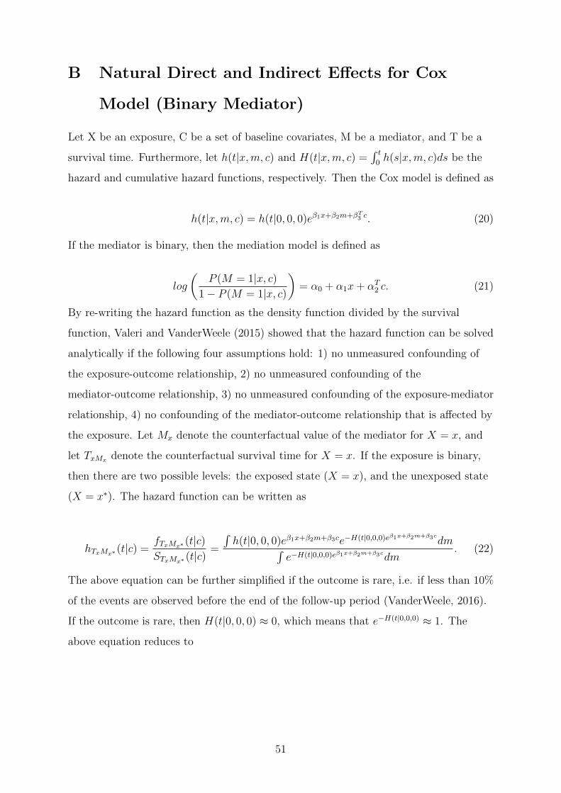
B Natural Direct and Indirect E↵ects for Cox
Model (Binary Mediator)
Let X be an exposure, C be a set of baseline covariates, M be a mediator, and T be a
survival time. Furthermore, let h(t|x,m, c) and H(t|x,m, c) =R t
0 h(s|x,m, c)ds be the
hazard and cumulative hazard functions, respectively. Then the Cox model is defined as
h(t|x,m, c) = h(t|0, 0, 0)e�1x+�2m+�T
3 c. (20)
If the mediator is binary, then the mediation model is defined as
log
✓P (M = 1|x, c)
1� P (M = 1|x, c)
◆= ↵0 + ↵1x+ ↵T
2 c. (21)
By re-writing the hazard function as the density function divided by the survival
function, Valeri and VanderWeele (2015) showed that the hazard function can be solved
analytically if the following four assumptions hold: 1) no unmeasured confounding of
the exposure-outcome relationship, 2) no unmeasured confounding of the
mediator-outcome relationship, 3) no unmeasured confounding of the exposure-mediator
relationship, 4) no confounding of the mediator-outcome relationship that is a↵ected by
the exposure. Let Mx denote the counterfactual value of the mediator for X = x, and
let TxMx
denote the counterfactual survival time for X = x. If the exposure is binary,
then there are two possible levels: the exposed state (X = x), and the unexposed state
(X = x⇤). The hazard function can be written as
hTx
Mx
⇤ (t|c) =fT
x
Mx
⇤ (t|c)ST
x
Mx
⇤ (t|c)=
Rh(t|0, 0, 0)e�1x+�2m+�3ce�H(t|0,0,0)e�1x+�2m+�3cdmR
e�H(t|0,0,0)e�1x+�2m+�3cdm. (22)
The above equation can be further simplified if the outcome is rare, i.e. if less than 10%
of the events are observed before the end of the follow-up period (VanderWeele, 2016).
If the outcome is rare, then H(t|0, 0, 0) ⇡ 0, which means that e�H(t|0,0,0) ⇡ 1. The
above equation reduces to
51

hTx
Mx
⇤ (t|c) =fT
x
Mx
⇤ (t|c)ST
x
Mx
⇤ (t|c)
⇡ h(t|0, 0, 0)e�1x+�3c
Ze�2mdm
⇡ h(t|0, 0, 0)e�1x+�3cE[e�2M ].
(23)
Recall that M is a binomial random variable with p = e↵0+↵1x+↵
T
2 c
1+e↵0+↵1x+↵
T
2 c
. Then, the moment
generating function is defined as
E[etM ] = 1� p+ pet. (24)
Thus, the hazard function can be re-written as
hTx
Mx
⇤ (t|c) ⇡ h(t|0, 0, 0)e�1x+�3cE[e�2M ]
⇡ h(t|0, 0, 0)e�1x+�3c
1� e↵0+↵1x⇤+↵T
2 c
1 + e↵0+↵1x⇤+↵T
2 c+
e↵0+↵1x⇤+↵T
2 c
1 + e↵0+↵1x⇤+↵T
2 ce�2
!
⇡ h(t|0, 0, 0)e�1x+�3c
1 + e↵0+↵1x⇤+↵T
2 c+�2
1 + e↵0+↵1x⇤+↵T
2 c
!.
(25)
Recall that the natural direct is defined as the di↵erence between the counterfactual
outcomes for an individual who is unexposed compared to the same individual who is
exposed, with the mediator set to the value it would normally take when the individual
is unexposed. Similarly, the natural indirect e↵ect is defined as the di↵erence between
the counterfactual outcomes for an individual with mediator set to the value it would
normally take when the individual is exposed compared to the same individual with
mediator set to the value it would normally take when the individual is unexposed. In
this case, the individual is assumed to be exposed. Finally, the total e↵ect is defined as
the di↵erence between the counterfactual outcome for an individual who is exposed
with the mediator set to the value it would normally take when an individual is exposed
compared to the same individual who is unexposed with the mediator set to the value it
would normally take when an individual is unexposed (Richiardi et al., 2013). Thus, the
natural direct e↵ect, the natural indirect e↵ect, and the total e↵ect can be summarized
on the hazard ratio scale when the survival time is rare.
52
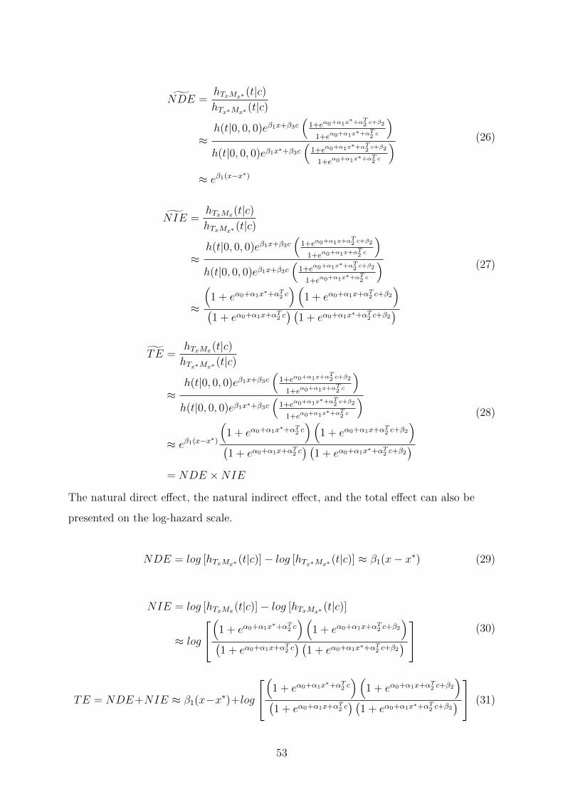
gNDE =hT
x
Mx
⇤ (t|c)hT
x
⇤Mx
⇤ (t|c)
⇡h(t|0, 0, 0)e�1x+�3c
⇣1+e↵0+↵1x
⇤+↵
T
2 c+�2
1+e↵0+↵1x⇤+↵
T
2 c
⌘
h(t|0, 0, 0)e�1x⇤+�3c⇣
1+e↵0+↵1x⇤+↵
T
2 c+�2
1+e↵0+↵1x⇤+↵
T
2 c
⌘
⇡ e�1(x�x⇤)
(26)
gNIE =hT
x
Mx
(t|c)hT
x
Mx
⇤ (t|c)
⇡h(t|0, 0, 0)e�1x+�3c
⇣1+e↵0+↵1x+↵
T
2 c+�2
1+e↵0+↵1x+↵
T
2 c
⌘
h(t|0, 0, 0)e�1x+�3c⇣
1+e↵0+↵1x⇤+↵
T
2 c+�2
1+e↵0+↵1x⇤+↵
T
2 c
⌘
⇡
⇣1 + e↵0+↵1x⇤+↵T
2 c⌘⇣
1 + e↵0+↵1x+↵T
2 c+�2
⌘
�1 + e↵0+↵1x+↵T
2 c� �
1 + e↵0+↵1x⇤+↵T
2 c+�2�
(27)
gTE =hT
x
Mx
(t|c)hT
x
⇤Mx
⇤ (t|c)
⇡h(t|0, 0, 0)e�1x+�3c
⇣1+e↵0+↵1x+↵
T
2 c+�2
1+e↵0+↵1x+↵
T
2 c
⌘
h(t|0, 0, 0)e�1x⇤+�3c⇣
1+e↵0+↵1x⇤+↵
T
2 c+�2
1+e↵0+↵1x⇤+↵
T
2 c
⌘
⇡ e�1(x�x⇤)
⇣1 + e↵0+↵1x⇤+↵T
2 c⌘⇣
1 + e↵0+↵1x+↵T
2 c+�2
⌘
�1 + e↵0+↵1x+↵T
2 c� �
1 + e↵0+↵1x⇤+↵T
2 c+�2�
= NDE ⇥NIE
(28)
The natural direct e↵ect, the natural indirect e↵ect, and the total e↵ect can also be
presented on the log-hazard scale.
NDE = log [hTx
Mx
⇤ (t|c)]� log [hTx
⇤Mx
⇤ (t|c)] ⇡ �1(x� x⇤) (29)
NIE = log [hTx
Mx
(t|c)]� log [hTx
Mx
⇤ (t|c)]
⇡ log
2
4
⇣1 + e↵0+↵1x⇤+↵T
2 c⌘⇣
1 + e↵0+↵1x+↵T
2 c+�2
⌘
�1 + e↵0+↵1x+↵T
2 c� �
1 + e↵0+↵1x⇤+↵T
2 c+�2�
3
5(30)
TE = NDE+NIE ⇡ �1(x�x⇤)+log
2
4
⇣1 + e↵0+↵1x⇤+↵T
2 c⌘⇣
1 + e↵0+↵1x+↵T
2 c+�2
⌘
�1 + e↵0+↵1x+↵T
2 c� �
1 + e↵0+↵1x⇤+↵T
2 c+�2�
3
5 (31)
53

C Natural Direct and Indirect E↵ects for Cox
Model (Continuous Mediator)
Let X be an exposure, C be a set of baseline covariates, M be a mediator, T be a
survival time. Furthermore, let h(t|x,m, c) and H(t|x,m, c) =R t
0 h(s|x,m, c)ds be the
hazard and cumulative hazard functions, respectively. Then the Cox model is defined as
h(t|x,m, c) = h(t|0, 0, 0)e�1x+�2m+�T
3 c. (32)
If the mediator is continuous and normally distributed, then the mediation model is
defined as
E[M |x, c] = ↵0 + ↵1x+ ↵T2 c. (33)
By re-writing the hazard function as the density function divided by the survival
function, VanderWeele (2011) showed that the hazard function can be solved
analytically if the following four assumptions hold: 1) no unmeasured confounding of
the exposure-outcome relationship, 2) no unmeasured confounding of the
mediator-outcome relationship, 2) no unmeasured confounding of the exposure-mediator
relationship, 4) no confounding of the mediator-outcome relationship that is a↵ected by
the exposure. Let Mx denote the counterfactual value of the mediator for X = x, and
let TxMx
denote the counterfactual survival time for X = x. If the exposure is binary,
then there are two possible levels: the exposed state (X = x), and the unexposed state
(X = x⇤). The hazard function can be written as
hTx
Mx
⇤ (t|c) =fT
x
Mx
⇤ (t|c)ST
x
Mx
⇤ (t|c)
= h(t|0, 0, 0)e�1x+�T
3 ce�2(↵0+↵1x⇤+↵T
2 c)+ 12�
22�
2
⇥ReH(t|0,0,0)e�
22+�1x+�2m+�
T
3 c
e�(m�(↵0+↵1x
⇤+↵
T
2 c))2
2 dmReH(t|0,0,0)e�1x+�2m+�
T
3 c
e�(m�(↵0+↵1x
⇤+↵
T
2 ))2
2 dm.
(34)
The above equation can be further simplified if the outcome is rare, i.e. if less than 10%
of the events are observed before the end of the follow-up period (VanderWeele, 2016).
If the outcome is rare, then H(t|0, 0, 0) ⇡ 0, which means that eH(t|0,0,0) ⇡ 1. The above
equation reduces to
54

hTx
Mx
⇤ (t|c) =fT
x
Mx
⇤ (t|c)ST
x
Mx
⇤ (t|c)
⇡ h(t|0, 0, 0)e�1x+�T
3 ce�2(↵0+↵1x⇤+↵T
2 c)+ 12�
22�
2 ⇥Re�
(m�(↵0+↵1x⇤+↵
T
2 c))2
2 dmRe�
(m�(↵0+↵1x⇤+↵
T
2 c))2
2 dm
⇡ h(t|0, 0, 0)e�1x+�T
3 ce�2(↵0+↵1x⇤+↵T
2 c)+ 12�
22�
2.
(35)
Thus, the log-hazard function is equal to
log [hTx
Mx
⇤ (t|c)] ⇡ loghh(t|0, 0, 0)e�1x+�T
3 ce�2(↵0+↵1x⇤+↵T
2 c)+ 12�
22�
2i
⇡ log [h(t|0, 0, 0)] + �1x+ �T3 c+ �2(↵0 + ↵1x
⇤ + ↵T2 c) +
1
2�22�
2.(36)
Recall that the natural direct is defined as the di↵erence between the counterfactual
outcomes for an individual who is unexposed compared to the same individual who is
exposed, with the mediator set to the value it would normally take when the individual
is unexposed. On the other hand, the natural indirect e↵ect is defined as the di↵erence
between the counterfactual outcomes for an individual with mediator set to the value it
would normally take when the individual is exposed compared to the same individual
with mediator set to the value it would normally take when the individual is unexposed.
In this case, the individual is assumed to be exposed. Finally, the total e↵ect is defined
as the di↵erence between the counterfactual outcome for an individual who is exposed
with the mediator set to the value it would normally take when an individual is exposed
compared to the same individual who is unexposed with the mediator set to the value it
would normally take when an individual is unexposed. On the log-hazard scale, the
total e↵ect is simply the sum of the natural direct and indirect e↵ects (Richiardi et al.,
2013). Thus, the natural direct e↵ect, the natural indirect e↵ect, and the total e↵ect
can be summarized on the log-hazard scale when the survival time is rare.
NDE = log [hTx
Mx
⇤ (t|c)]� log [hTx
⇤Mx
⇤ (t|c)] ⇡ �1(x� x⇤) (37)
NIE = log [hTx
Mx
(t|c)]� log [hTx
Mx
⇤ (t|c)] ⇡ �2↵1(x� x⇤) (38)
TE = NDE +NIE = log [hTx
Mx
(t|c)]� log [hTx
⇤Mx
⇤ (t|c)] ⇡ (�2↵1 + �1)(x� x⇤) (39)
55

D Coverage Rates (Binary Mediator)
Coverage of the 95% confidence interval for both the natural direct and indirect e↵ects
for the binary mediator are presented in the following tables.
Coverage of 95% confidence interval for NDE
Stratum: 5.3%, Cluster: 10.3%
Variance Estimator Unweighted CovariateScaled
WeightedHybrid
Robust Model-Based 0.9580 0.9600 0.9520 0.9500
Design-Based 0.9490 0.9470 0.9380 0.9380
Partial Bootstrap 0.9470 0.9490 0.9410 0.9390
Full Bootstrap 0.9410 0.9380 0.9350 0.9360
Stratum: 2.0%, Cluster: 10.3%
Variance Estimator Unweighted CovariateScaled
WeightedHybrid
Robust Model-Based 0.9530 0.9530 0.9510 0.9500
Design-Based 0.9460 0.9480 0.9480 0.9460
Partial Bootstrap 0.9470 0.9470 0.9470 0.9460
Full Bootstrap 0.9360 0.9370 0.9400 0.9400
Stratum: 0.2%, Cluster: 10.3%
Variance Estimator Unweighted CovariateScaled
WeightedHybrid
Robust Model-Based 0.9510 0.9500 0.9570 0.9560
Design-Based 0.9410 0.9410 0.9390 0.9370
Partial Bootstrap 0.9430 0.9410 0.9410 0.9450
Full Bootstrap 0.9370 0.9380 0.9310 0.9330
56

Stratum: 10.3%, Cluster: 5.3%
Variance Estimator Unweighted CovariateScaled
WeightedHybrid
Robust Model-Based 0.9530 0.9530 0.9460 0.9450
Design-Based 0.9410 0.9420 0.9380 0.9410
Partial Bootstrap 0.9450 0.9470 0.9390 0.9440
Full Bootstrap 0.9390 0.9400 0.9330 0.9350
Stratum: 10.3%, Cluster: 2.0%
Variance Estimator Unweighted CovariateScaled
WeightedHybrid
Robust Model-Based 0.9580 0.9580 0.9510 0.9470
Design-Based 0.9450 0.9430 0.9470 0.9400
Partial Bootstrap 0.9460 0.9450 0.9460 0.9450
Full Bootstrap 0.9390 0.9390 0.9400 0.9400
Stratum: 10.3%, Cluster: 0.2%
Variance Estimator Unweighted CovariateScaled
WeightedHybrid
Robust Model-Based 0.9570 0.9570 0.9540 0.9520
Design-Based 0.9530 0.9510 0.9520 0.9500
Partial Bootstrap 0.9550 0.9550 0.9550 0.9520
Full Bootstrap 0.9500 0.9480 0.9450 0.9440
57
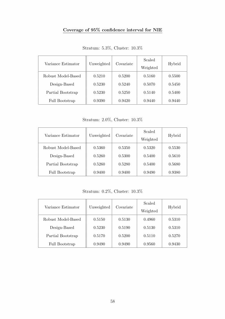
Coverage of 95% confidence interval for NIE
Stratum: 5.3%, Cluster: 10.3%
Variance Estimator Unweighted CovariateScaled
WeightedHybrid
Robust Model-Based 0.5210 0.5200 0.5160 0.5500
Design-Based 0.5230 0.5240 0.5070 0.5450
Partial Bootstrap 0.5230 0.5250 0.5140 0.5400
Full Bootstrap 0.9390 0.9420 0.9440 0.9440
Stratum: 2.0%, Cluster: 10.3%
Variance Estimator Unweighted CovariateScaled
WeightedHybrid
Robust Model-Based 0.5360 0.5350 0.5320 0.5530
Design-Based 0.5260 0.5300 0.5400 0.5610
Partial Bootstrap 0.5260 0.5280 0.5400 0.5680
Full Bootstrap 0.9400 0.9400 0.9490 0.9380
Stratum: 0.2%, Cluster: 10.3%
Variance Estimator Unweighted CovariateScaled
WeightedHybrid
Robust Model-Based 0.5150 0.5130 0.4960 0.5310
Design-Based 0.5230 0.5190 0.5130 0.5310
Partial Bootstrap 0.5170 0.5200 0.5110 0.5270
Full Bootstrap 0.9490 0.9490 0.9560 0.9430
58

Stratum: 10.3%, Cluster: 5.3%
Variance Estimator Unweighted CovariateScaled
WeightedHybrid
Robust Model-Based 0.5160 0.5110 0.5160 0.5350
Design-Based 0.5090 0.5050 0.5130 0.5340
Partial Bootstrap 0.5110 0.5070 0.5100 0.5370
Full Bootstrap 0.9410 0.9410 0.9460 0.9450
Stratum: 10.3%, Cluster: 2.0%
Variance Estimator Unweighted CovariateScaled
WeightedHybrid
Robust Model-Based 0.4810 0.4850 0.4880 0.5270
Design-Based 0.4750 0.4770 0.4820 0.5070
Partial Bootstrap 0.4790 0.4810 0.4780 0.5100
Full Bootstrap 0.9420 0.9420 0.9420 0.9460
Stratum: 10.3%, Cluster: 0.2%
Variance Estimator Unweighted CovariateScaled
WeightedHybrid
Robust Model-Based 0.5160 0.5150 0.5290 0.5450
Design-Based 0.5250 0.5220 0.5240 0.5410
Partial Bootstrap 0.5240 0.5200 0.5250 0.5400
Full Bootstrap 0.9430 0.9430 0.9380 0.9450
59

E Coverage Rates (Continuous Mediator)
Coverage of the 95% confidence interval for both the natural direct and indirect e↵ects
for the continuous mediator are presented in the following tables.
Coverage of 95% confidence interval for NDE
Stratum: 5.3%, Cluster: 10.3%
Variance Estimate Unweighted CovariateScaled
WeightedHybrid
Unscaled
Weighted
Robust Model-Based 0.9460 0.9460 0.9520 0.9480 0.3160
Design-Based 0.9340 0.9340 0.9390 0.9390 0.3150
Partial Bootstrap 0.9350 0.9380 0.9440 0.9420 0.3300
Unscaled Full Bootstrap 0.9230 0.9250 – 0.9270 0.3290
Scaled Full Bootstrap 0.9270 0.9260 0.9340 0.9340 –
Stratum: 2.0%, Cluster: 10.3%
Variance Estimate Unweighted CovariateScaled
WeightedHybrid
Unscaled
Weighted
Robust Model-Based 0.9510 0.9490 0.9460 0.9470 0.3340
Design-Based 0.9430 0.9420 0.9380 0.9430 0.3230
Partial Bootstrap 0.9450 0.9450 0.9450 0.9460 0.3270
Unscaled Full Bootstrap 0.9300 0.9290 – 0.9300 0.3270
Scaled Full Bootstrap 0.9360 0.9350 0.9320 0.9310 –
60

Stratum: 0.2%, Cluster: 10.3%
Variance Estimate Unweighted CovariateScaled
WeightedHybrid
Unscaled
Weighted
Robust Model-Based 0.9550 0.9550 0.9560 0.9560 0.3690
Design-Based 0.9440 0.9440 0.9460 0.9440 0.3760
Partial Bootstrap 0.9480 0.9480 0.9500 0.9480 0.3840
Unscaled Full Bootstrap 0.9360 0.9350 – 0.9310 0.3830
Scaled Full Bootstrap 0.9380 0.9360 0.9400 0.9390 –
Stratum: 10.3%, Cluster: 5.3%
Variance Estimate Unweighted CovariateScaled
WeightedHybrid
Unscaled
Weighted
Robust Model-Based 0.9530 0.9530 0.9620 0.9580 0.3240
Design-Based 0.9430 0.9430 0.9550 0.9530 0.3150
Partial Bootstrap 0.9460 0.9450 0.9580 0.9550 0.3220
Unscaled Full Bootstrap 0.9270 0.9290 – 0.9340 0.3220
Scaled Full Bootstrap 0.9330 0.9310 0.9440 0.9460 –
Stratum: 10.3%, Cluster: 2.0%
Variance Estimate Unweighted CovariateScaled
WeightedHybrid
Unscaled
Weighted
Robust Model-Based 0.9500 0.9500 0.9520 0.9490 0.3420
Design-Based 0.9490 0.9490 0.9520 0.9520 0.3550
Partial Bootstrap 0.9500 0.9490 0.9520 0.9540 0.3630
Unscaled Full Bootstrap 0.9350 0.9340 – 0.9360 0.3630
Scaled Full Bootstrap 0.9360 0.9360 0.9450 0.9450 –
61

Stratum: 10.3%, Cluster: 0.2%
Variance Estimate Unweighted CovariateScaled
WeightedHybrid
Unscaled
Weighted
Robust Model-Based 0.9530 0.9540 0.9460 0.9450 0.2770
Design-Based 0.9450 0.9450 0.9450 0.9390 0.2850
Partial Bootstrap 0.9440 0.9430 0.9420 0.9410 0.2900
Unscaled Full Bootstrap 0.9330 0.9320 – 0.9300 0.2900
Scaled Full Bootstrap 0.9370 0.9400 0.9360 0.9310 –
Coverage of 95% confidence interval for NIE
Stratum: 5.3%, Cluster: 10.3%
Variance Estimate Unweighted CovariateScaled
WeightedHybrid
Unscaled
Weighted
Robust Model-Based 0.5450 0.5450 0.5470 0.5630 0.0000
Design-Based 0.5310 0.5290 0.5340 0.5460 0.0000
Partial Bootstrap 0.5330 0.5310 0.5370 0.5540 0.0000
Unscaled Full Bootstrap 0.7990 0.7990 – 0.8040 0.0000
Scaled Full Bootstrap 0.9230 0.9240 0.9360 0.9210 –
Stratum: 2.0%, Cluster: 10.3%
Variance Estimate Unweighted CovariateScaled
WeightedHybrid
Unscaled
Weighted
Robust Model-Based 0.5300 0.5260 0.5130 0.5520 0.0000
Design-Based 0.5130 0.5140 0.5050 0.5390 0.0000
Partial Bootstrap 0.5160 0.5150 0.5040 0.5410 0.0000
Unscaled Full Bootstrap 0.8190 0.8190 – 0.8180 0.0000
Scaled Full Bootstrap 0.9430 0.9430 0.9330 0.9390 –
62
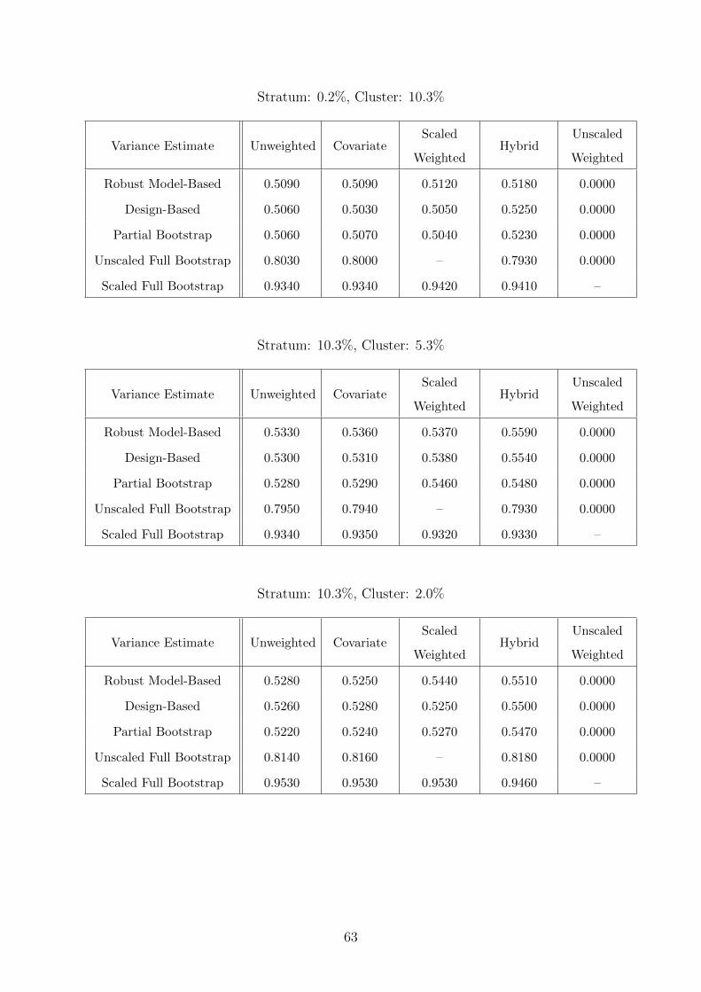
Stratum: 0.2%, Cluster: 10.3%
Variance Estimate Unweighted CovariateScaled
WeightedHybrid
Unscaled
Weighted
Robust Model-Based 0.5090 0.5090 0.5120 0.5180 0.0000
Design-Based 0.5060 0.5030 0.5050 0.5250 0.0000
Partial Bootstrap 0.5060 0.5070 0.5040 0.5230 0.0000
Unscaled Full Bootstrap 0.8030 0.8000 – 0.7930 0.0000
Scaled Full Bootstrap 0.9340 0.9340 0.9420 0.9410 –
Stratum: 10.3%, Cluster: 5.3%
Variance Estimate Unweighted CovariateScaled
WeightedHybrid
Unscaled
Weighted
Robust Model-Based 0.5330 0.5360 0.5370 0.5590 0.0000
Design-Based 0.5300 0.5310 0.5380 0.5540 0.0000
Partial Bootstrap 0.5280 0.5290 0.5460 0.5480 0.0000
Unscaled Full Bootstrap 0.7950 0.7940 – 0.7930 0.0000
Scaled Full Bootstrap 0.9340 0.9350 0.9320 0.9330 –
Stratum: 10.3%, Cluster: 2.0%
Variance Estimate Unweighted CovariateScaled
WeightedHybrid
Unscaled
Weighted
Robust Model-Based 0.5280 0.5250 0.5440 0.5510 0.0000
Design-Based 0.5260 0.5280 0.5250 0.5500 0.0000
Partial Bootstrap 0.5220 0.5240 0.5270 0.5470 0.0000
Unscaled Full Bootstrap 0.8140 0.8160 – 0.8180 0.0000
Scaled Full Bootstrap 0.9530 0.9530 0.9530 0.9460 –
63

Stratum: 10.3%, Cluster: 0.2%
Variance Estimate Unweighted CovariateScaled
WeightedHybrid
Unscaled
Weighted
Robust Model-Based 0.5550 0.5530 0.5440 0.5810 0.0000
Design-Based 0.5400 0.5420 0.5320 0.5650 0.0000
Partial Bootstrap 0.5420 0.5430 0.5360 0.5670 0.0000
Unscaled Full Bootstrap 0.8380 0.8390 – 0.8210 0.0000
Scaled Full Bootstrap 0.9450 0.9440 0.9410 0.9370 –
64
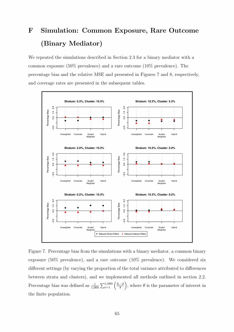
F Simulation: Common Exposure, Rare Outcome
(Binary Mediator)
We repeated the simulations described in Section 2.3 for a binary mediator with a
common exposure (50% prevalence) and a rare outcome (10% prevalence). The
percentage bias and the relative MSE and presented in Figures 7 and 8, respectively,
and coverage rates are presented in the subsequent tables.
●
Stratum: 5.3%, Cluster: 10.3%
Perc
enta
ge B
ias
● ●
● ●
Unweighted Covariate ScaledWeighted
Hybrid
−3.0
0.0
1.5
3.0
●
Stratum: 2.0%, Cluster: 10.3%
Perc
enta
ge B
ias
● ●● ●
Unweighted Covariate ScaledWeighted
Hybrid
−3.0
0.0
1.5
3.0
Stratum: 0.2%, Cluster: 10.3%
Perc
enta
ge B
ias
● ●● ●
Unweighted Covariate ScaledWeighted
Hybrid
−3.0
0.0
1.5
3.0
●
Stratum: 10.3%, Cluster: 5.3%
Perc
enta
ge B
ias
● ● ● ●
Unweighted Covariate ScaledWeighted
Hybrid
−3.0
0.0
1.5
3.0
●
Stratum: 10.3%, Cluster: 2.0%
Perc
enta
ge B
ias
● ●● ●
Unweighted Covariate ScaledWeighted
Hybrid
−3.0
0.0
1.5
3.0
Stratum: 10.3%, Cluster: 0.2%
Perc
enta
ge B
ias
● ● ● ●
Unweighted Covariate ScaledWeighted
Hybrid
−3.0
0.0
1.5
3.0
● Natural Direct Effect Natural Indirect Effect
Figure 7. Percentage bias from the simulations with a binary mediator, a common binary
exposure (50% prevalence), and a rare outcome (10% prevalence). We considered six
di↵erent settings (by varying the proportion of the total variance attributed to di↵erences
between strata and clusters), and we implemented all methods outlined in section 2.2.
Percentage bias was defined as 11,000
P1,000i=1
⇣✓i
�✓✓
⌘, where ✓ is the parameter of interest in
the finite population.
65
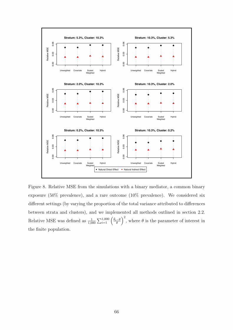
Stratum: 5.3%, Cluster: 10.3%
Rel
ative
MSE
● ●● ●
Unweighted Covariate ScaledWeighted
Hybrid
0.00
0.03
0.06
Stratum: 2.0%, Cluster: 10.3%
Rel
ative
MSE
● ●● ●
Unweighted Covariate ScaledWeighted
Hybrid
0.00
0.03
0.06
Stratum: 0.2%, Cluster: 10.3%
Rel
ative
MSE
● ●● ●
Unweighted Covariate ScaledWeighted
Hybrid
0.00
0.03
0.06
Stratum: 10.3%, Cluster: 5.3%
Rel
ative
MSE
● ●● ●
Unweighted Covariate ScaledWeighted
Hybrid
0.00
0.03
0.06
Stratum: 10.3%, Cluster: 2.0%
Rel
ative
MSE ● ●
● ●
Unweighted Covariate ScaledWeighted
Hybrid
0.00
0.03
0.06
Stratum: 10.3%, Cluster: 0.2%
Rel
ative
MSE ● ●
● ●
Unweighted Covariate ScaledWeighted
Hybrid
0.00
0.03
0.06
● Natural Direct Effect Natural Indirect Effect
Figure 8. Relative MSE from the simulations with a binary mediator, a common binary
exposure (50% prevalence), and a rare outcome (10% prevalence). We considered six
di↵erent settings (by varying the proportion of the total variance attributed to di↵erences
between strata and clusters), and we implemented all methods outlined in section 2.2.
Relative MSE was defined as 11,000
P1,000i=1
⇣✓i
�✓✓
⌘2, where ✓ is the parameter of interest in
the finite population.
66
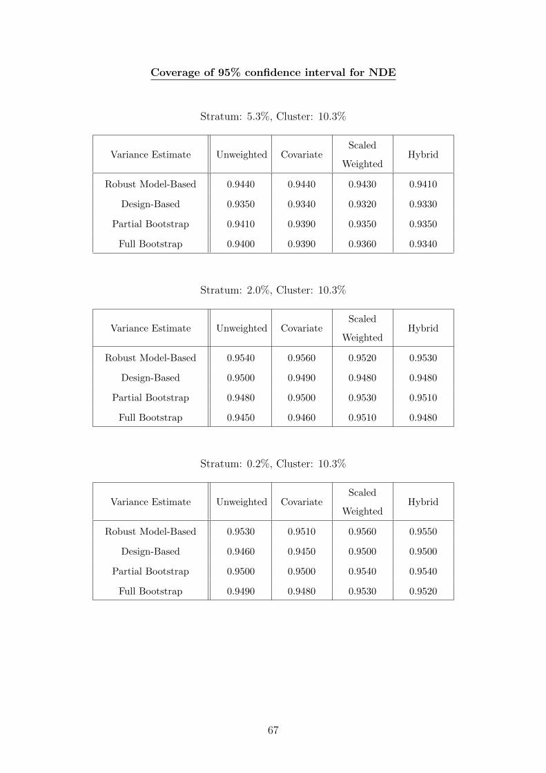
Coverage of 95% confidence interval for NDE
Stratum: 5.3%, Cluster: 10.3%
Variance Estimate Unweighted CovariateScaled
WeightedHybrid
Robust Model-Based 0.9440 0.9440 0.9430 0.9410
Design-Based 0.9350 0.9340 0.9320 0.9330
Partial Bootstrap 0.9410 0.9390 0.9350 0.9350
Full Bootstrap 0.9400 0.9390 0.9360 0.9340
Stratum: 2.0%, Cluster: 10.3%
Variance Estimate Unweighted CovariateScaled
WeightedHybrid
Robust Model-Based 0.9540 0.9560 0.9520 0.9530
Design-Based 0.9500 0.9490 0.9480 0.9480
Partial Bootstrap 0.9480 0.9500 0.9530 0.9510
Full Bootstrap 0.9450 0.9460 0.9510 0.9480
Stratum: 0.2%, Cluster: 10.3%
Variance Estimate Unweighted CovariateScaled
WeightedHybrid
Robust Model-Based 0.9530 0.9510 0.9560 0.9550
Design-Based 0.9460 0.9450 0.9500 0.9500
Partial Bootstrap 0.9500 0.9500 0.9540 0.9540
Full Bootstrap 0.9490 0.9480 0.9530 0.9520
67

Stratum: 10.3%, Cluster: 5.3%
Variance Estimate Unweighted CovariateScaled
WeightedHybrid
Robust Model-Based 0.9510 0.9510 0.9540 0.9530
Design-Based 0.9410 0.9410 0.9480 0.9480
Partial Bootstrap 0.9430 0.9430 0.9510 0.9500
Full Bootstrap 0.9430 0.9440 0.9490 0.9490
Stratum: 10.3%, Cluster: 2.0%
Variance Estimate Unweighted CovariateScaled
WeightedHybrid
Robust Model-Based 0.9540 0.9540 0.9610 0.9620
Design-Based 0.9390 0.9410 0.9490 0.9490
Partial Bootstrap 0.9420 0.9440 0.9470 0.9470
Full Bootstrap 0.9400 0.9420 0.9460 0.9450
Stratum: 10.3%, Cluster: 0.2%
Variance Estimate Unweighted CovariateScaled
WeightedHybrid
Robust Model-Based 0.9620 0.9630 0.9610 0.9600
Design-Based 0.9560 0.9550 0.9580 0.9590
Partial Bootstrap 0.9570 0.9570 0.9620 0.9640
Full Bootstrap 0.9550 0.9520 0.9580 0.9630
68

Coverage of 95% confidence interval for NIE
Stratum: 5.3%, Cluster: 10.3%
Variance Estimate Unweighted CovariateScaled
WeightedHybrid
Robust Model-Based 0.8800 0.8800 0.8710 0.8880
Design-Based 0.8870 0.8850 0.8700 0.8840
Partial Bootstrap 0.8850 0.8860 0.8690 0.8830
Full Bootstrap 0.9400 0.9400 0.9250 0.9330
Stratum: 2.0%, Cluster: 10.3%
Variance Estimate Unweighted CovariateScaled
WeightedHybrid
Robust Model-Based 0.8930 0.8920 0.8900 0.8970
Design-Based 0.8830 0.8810 0.8830 0.8920
Partial Bootstrap 0.8870 0.8870 0.8840 0.8920
Full Bootstrap 0.9350 0.9350 0.9380 0.9410
Stratum: 0.2%, Cluster: 10.3%
Variance Estimate Unweighted CovariateScaled
WeightedHybrid
Robust Model-Based 0.9090 0.9080 0.8970 0.9070
Design-Based 0.9010 0.8970 0.8860 0.8960
Partial Bootstrap 0.9020 0.9040 0.8880 0.9030
Full Bootstrap 0.9560 0.9550 0.9420 0.9520
69

Stratum: 10.3%, Cluster: 5.3%
Variance Estimate Unweighted CovariateScaled
WeightedHybrid
Robust Model-Based 0.8840 0.8820 0.8780 0.8970
Design-Based 0.8800 0.8790 0.8820 0.8890
Partial Bootstrap 0.8750 0.8770 0.8840 0.8920
Full Bootstrap 0.9330 0.9330 0.9350 0.9360
Stratum: 10.3%, Cluster: 2.0%
Variance Estimate Unweighted CovariateScaled
WeightedHybrid
Robust Model-Based 0.9020 0.9000 0.9090 0.9170
Design-Based 0.8940 0.8940 0.9060 0.9100
Partial Bootstrap 0.8950 0.8950 0.9060 0.9100
Full Bootstrap 0.9480 0.9460 0.9440 0.9500
Stratum: 10.3%, Cluster: 0.2%
Variance Estimate Unweighted CovariateScaled
WeightedHybrid
Robust Model-Based 0.8830 0.8790 0.8810 0.8900
Design-Based 0.8720 0.8750 0.8720 0.8730
Partial Bootstrap 0.8690 0.8730 0.8770 0.8750
Full Bootstrap 0.9400 0.9350 0.9400 0.9440
70

G Simulation: Common Exposure, Rare Outcome
(Continuous Mediator)
We repeated the simulations described in Section 2.3 for a continuous mediator with a
common exposure (50% prevalence) and a rare outcome (10% prevalence). The
percentage bias and the relative MSE and presented in Figures 9 and 10, respectively,
and coverage rates are presented in the subsequent tables.
●
Stratum: 5.3%, Cluster: 10.3%
Perc
enta
ge B
ias
● ● ● ●
●
Unweighted Covariate ScaledWeighted
Hybrid UnscaledWeighted
−100
−50
050
100
Stratum: 2.0%, Cluster: 10.3%
Perc
enta
ge B
ias
● ● ● ●
●
Unweighted Covariate ScaledWeighted
Hybrid UnscaledWeighted
−100
−50
050
100
Stratum: 0.2%, Cluster: 10.3%
Perc
enta
ge B
ias
● ● ● ●
●
Unweighted Covariate ScaledWeighted
Hybrid UnscaledWeighted
−100
−50
050
100
●
Stratum: 10.3%, Cluster: 5.3%
Perc
enta
ge B
ias
● ● ● ●
●
Unweighted Covariate ScaledWeighted
Hybrid UnscaledWeighted
−100
−50
050
100
Stratum: 10.3%, Cluster: 2.0%
Perc
enta
ge B
ias
● ● ● ●
●
Unweighted Covariate ScaledWeighted
Hybrid UnscaledWeighted
−100
−50
050
100
Stratum: 10.3%, Cluster: 0.2%
Perc
enta
ge B
ias
● ● ● ●
●
Unweighted Covariate ScaledWeighted
Hybrid UnscaledWeighted
−100
−50
050
100
● Natural Direct Effect Natural Indirect Effect
Figure 9. Percentage bias from the simulations with a continuous mediator, a common
binary exposure (50% prevalence), and a rare outcome (10% prevalence). We consid-
ered six di↵erent settings (by varying the proportion of the total variance attributed to
di↵erences between strata and clusters), and we implemented all methods outlined in
section 2.2. Percentage bias was defined as 11,000
P1,000i=1
⇣✓i
�✓✓
⌘, where ✓ is the parameter
of interest in the finite population.
71

Stratum: 5.3%, Cluster: 10.3%
Rel
ative
MSE
● ● ● ●
●
Unweighted Covariate ScaledWeighted
Hybrid UnscaledWeighted
0.0
0.5
1.0
Stratum: 2.0%, Cluster: 10.3%
Rel
ative
MSE
● ● ● ●
●
Unweighted Covariate ScaledWeighted
Hybrid UnscaledWeighted
0.0
0.5
1.0
Stratum: 0.2%, Cluster: 10.3%
Rel
ative
MSE
● ● ● ●
●
Unweighted Covariate ScaledWeighted
Hybrid UnscaledWeighted
0.0
0.5
1.0
Stratum: 10.3%, Cluster: 5.3%
Rel
ative
MSE
● ● ● ●
●
Unweighted Covariate ScaledWeighted
Hybrid UnscaledWeighted
0.0
0.5
1.0
Stratum: 10.3%, Cluster: 2.0%
Rel
ative
MSE
● ● ● ●
●
Unweighted Covariate ScaledWeighted
Hybrid UnscaledWeighted
0.0
0.5
1.0
Stratum: 10.3%, Cluster: 0.2%
Rel
ative
MSE
● ● ● ●
●
Unweighted Covariate ScaledWeighted
Hybrid UnscaledWeighted
0.0
0.5
1.0
● Natural Direct Effect Natural Indirect Effect
Figure 10. Relative MSE from the simulations with a continuous mediator, a common
binary exposure (50% prevalence), and a rare outcome (10% prevalence). We considered
six di↵erent settings (by varying the proportion of the total variance attributed to di↵er-
ences between strata and clusters), and we implemented all methods outlined in section
2.2. Relative MSE was defined as 11,000
P1,000i=1
⇣✓i
�✓✓
⌘2, where ✓ is the parameter of interest
in the finite population.
72

Coverage of 95% confidence interval for NDE
Stratum: 5.3%, Cluster: 10.3%
Variance Estimate Unweighted CovariateScaled
WeightedHybrid
Unscaled
Weighted
Robust Model-Based 0.9570 0.9570 0.9610 0.9620 0.5170
Design-Based 0.9520 0.9550 0.9540 0.9520 0.5140
Partial Bootstrap 0.9530 0.9530 0.9530 0.9570 0.5200
Unscaled Full Bootstrap 0.9470 0.9480 – 0.9470 0.5200
Scaled Full Bootstrap 0.9500 0.9500 0.9530 0.9530 –
Stratum: 2.0%, Cluster: 10.3%
Variance Estimate Unweighted CovariateScaled
WeightedHybrid
Unscaled
Weighted
Robust Model-Based 0.9520 0.9520 0.9530 0.9570 0.5260
Design-Based 0.9380 0.9400 0.9380 0.9420 0.5020
Partial Bootstrap 0.9400 0.9380 0.9420 0.9470 0.5130
Unscaled Full Bootstrap 0.9340 0.9340 – 0.9350 0.5130
Scaled Full Bootstrap 0.9380 0.9390 0.9450 0.9410 –
Stratum: 0.2%, Cluster: 10.3%
Variance Estimate Unweighted CovariateScaled
WeightedHybrid
Unscaled
Weighted
Robust Model-Based 0.9370 0.9390 0.9340 0.9380 0.5000
Design-Based 0.9300 0.9330 0.9260 0.9310 0.4920
Partial Bootstrap 0.9400 0.9420 0.9340 0.9360 0.5040
Unscaled Full Bootstrap 0.9320 0.9340 – 0.9300 0.5040
Scaled Full Bootstrap 0.9370 0.9380 0.9350 0.9350 –
73

Stratum: 10.3%, Cluster: 5.3%
Variance Estimate Unweighted CovariateScaled
WeightedHybrid
Unscaled
Weighted
Robust Model-Based 0.9560 0.9540 0.9520 0.9510 0.4970
Design-Based 0.9450 0.9460 0.9430 0.9440 0.4930
Partial Bootstrap 0.9490 0.9490 0.9510 0.9470 0.5070
Unscaled Full Bootstrap 0.9420 0.9440 – 0.9390 0.5070
Scaled Full Bootstrap 0.9470 0.9470 0.9440 0.9450 –
Stratum: 10.3%, Cluster: 2.0%
Variance Estimate Unweighted CovariateScaled
WeightedHybrid
Unscaled
Weighted
Robust Model-Based 0.9460 0.9460 0.9450 0.9430 0.5230
Design-Based 0.9320 0.9320 0.9380 0.9380 0.5260
Partial Bootstrap 0.9380 0.9370 0.9410 0.9410 0.5340
Unscaled Full Bootstrap 0.9290 0.9300 – 0.9310 0.5330
Scaled Full Bootstrap 0.9350 0.9330 0.9360 0.9390 –
Stratum: 10.3%, Cluster: 0.2%
Variance Estimate Unweighted CovariateScaled
WeightedHybrid
Unscaled
Weighted
Robust Model-Based 0.9390 0.9390 0.9430 0.9400 0.4890
Design-Based 0.9330 0.9350 0.9360 0.9330 0.4940
Partial Bootstrap 0.9370 0.9380 0.9380 0.9360 0.5070
Unscaled Full Bootstrap 0.9290 0.9310 – 0.9330 0.5070
Scaled Full Bootstrap 0.9330 0.9340 0.9370 0.9370 –
74

Coverage of 95% confidence interval for NIE
Stratum: 5.3%, Cluster: 10.3%
Variance Estimate Unweighted CovariateScaled
WeightedHybrid
Unscaled
Weighted
Robust Model-Based 0.8910 0.8900 0.9030 0.9060 0.0000
Design-Based 0.8790 0.8790 0.8910 0.8940 0.0000
Partial Bootstrap 0.8810 0.8790 0.8950 0.8930 0.0000
Unscaled Full Bootstrap 0.7980 0.7950 – 0.7960 0.0000
Scaled Full Bootstrap 0.9330 0.9340 0.9400 0.9360 –
Stratum: 2.0%, Cluster: 10.3%
Variance Estimate Unweighted CovariateScaled
WeightedHybrid
Unscaled
Weighted
Robust Model-Based 0.8980 0.8970 0.9040 0.9080 0.0000
Design-Based 0.8900 0.8870 0.8910 0.8980 0.0000
Partial Bootstrap 0.8930 0.8910 0.8920 0.8990 0.0000
Unscaled Full Bootstrap 0.7980 0.7980 – 0.7880 0.0000
Scaled Full Bootstrap 0.9390 0.9360 0.9360 0.9370 –
Stratum: 0.2%, Cluster: 10.3%
Variance Estimate Unweighted CovariateScaled
WeightedHybrid
Unscaled
Weighted
Robust Model-Based 0.9010 0.9020 0.9010 0.8990 0.0000
Design-Based 0.9020 0.9010 0.8940 0.8970 0.0000
Partial Bootstrap 0.9020 0.9040 0.8970 0.9050 0.0000
Unscaled Full Bootstrap 0.8020 0.8010 – 0.8020 0.0000
Scaled Full Bootstrap 0.9380 0.9380 0.9360 0.9330 –
75

Stratum: 10.3%, Cluster: 5.3%
Variance Estimate Unweighted CovariateScaled
WeightedHybrid
Unscaled
Weighted
Robust Model-Based 0.9250 0.9230 0.9130 0.9250 0.0000
Design-Based 0.9080 0.9070 0.9050 0.9120 0.0000
Partial Bootstrap 0.9070 0.9100 0.9030 0.9130 0.0000
Unscaled Full Bootstrap 0.8160 0.8150 – 0.8020 0.0000
Scaled Full Bootstrap 0.9580 0.9570 0.9510 0.9490 –
Stratum: 10.3%, Cluster: 2.0%
Variance Estimate Unweighted CovariateScaled
WeightedHybrid
Unscaled
Weighted
Robust Model-Based 0.9110 0.9100 0.9080 0.9130 0.0000
Design-Based 0.8970 0.8930 0.9030 0.9060 0.0000
Partial Bootstrap 0.8970 0.8930 0.9090 0.9080 0.0000
Unscaled Full Bootstrap 0.7960 0.7950 – 0.8060 0.0000
Scaled Full Bootstrap 0.9410 0.9430 0.9440 0.9440 –
Stratum: 10.3%, Cluster: 0.2%
Variance Estimate Unweighted CovariateScaled
WeightedHybrid
Unscaled
Weighted
Robust Model-Based 0.8850 0.8870 0.8940 0.8970 0.0000
Design-Based 0.8780 0.8800 0.8880 0.8910 0.0000
Partial Bootstrap 0.8790 0.8780 0.8920 0.8910 0.0000
Unscaled Full Bootstrap 0.7810 0.7880 – 0.7950 0.0000
Scaled Full Bootstrap 0.9280 0.9280 0.9350 0.9360 –
76

H Variance of Regression Coe�cients
In this appendix, we consider the variance of regression coe�cients in both linear and
logistic models.
Linear Model
Consider the following linear model, where X is binary and Y is continuous and
normally distributed:
E[Y |X] = �0 + �1X. (40)
The maximum likelihood estimate of �1 can be found by maximizing the log-likelihood
function, as shown in equations 41 and 42.
@l(�0, �1)
@�0=
@
@�
"nX
i=1
✓�(yi � (�0 + �1xi))2
2�2� 1
2log(2⇡�2)
◆#
=nX
i=1
@
@�0
✓�(yi � (�0 + �1xi))2
2�2� 1
2log(2⇡�2)
◆
=nX
i=1
yi � (�0 + �1xi)
�2= 0 ! �0 = y � �1x
(41)
@l(�0, �1)
@�1=
@
@�
"nX
i=1
✓�(yi � (�0 + �1xi))2
2�2� 1
2log(2⇡�2)
◆#
=nX
i=1
@
@�1
✓�(yi � (�0 + �1xi))2
2�2� 1
2log(2⇡�2)
◆
=nX
i=1
yi � xi(�0 + �1xi)
�2=
nX
i=1
xi
✓yi � (�0 + �1xi)
�2
◆
=nX
i=1
xiyi � xi�0 � �1x2i
�2= 0 ! �1 =
Pni=1 xiyi � �0
Pni=1 xiPn
i=1 x2i
(42)
We can substitute �0 from equation 41 into �1 from equation 42 to get
�1 =P
n
i=1(xi
�x)(yi
�y)Pn
i=1(xi
�x)2 (Rice, 2007). The variance of �1 is equal to
V ar(�1) = V ar⇣P
n
i=1(xi
�x)(yi
�y)Pn
i=1(xi
�x)2
⌘. Since yi = �0 + �1xi and y = �0 + �1x, the variance
of �1 can be re-written as V ar(�1) = V ar⇣P
n
i=1(xi
�x)(�1xi
��1x+✏)Pn
i=1(xi
�x)2
⌘, which can be further
reduced to V ar(�1) = V ar⇣�1 +
✏P
n
i=1(xi
�x)Pn
i=1(xi
�x)2
⌘. Finally, since V ar(X + c) = V ar(X) and
V ar(kX) = k2V ar(X), the variance of �1 is equal to V ar(�1) =�2
Pn
i=1(xi
�x)2 .
77

Let X be a binary variable with probability of success p, i.e. X ⇠ Bin(n, p). Then the
termPn
i=1(x� x)2 is maximized when p = 0.5. Thus, the variance of X is minimized
when p = 0.5.
Logistic Model
Consider the following logistic model, where X and Y are both binary:
log
✓P (Y = 1)
1� P (Y = 1)
◆= �0 + �1X (43)
The large-sample variances of �0 and �1 are given by the terms along the main diagonal
of the variance-covariance matrix. To obtain these terms, we first need to solve the
information matrix. To do so, let Y1 ⇠ Bin(m1, ⇡1) and Y2 ⇠ Bin(m2, ⇡2) be two
independent random variables. Then the information matrix can be found by
maximizing the log-likelihood function, i.e.
I(�) = �
@2l(�)
@�i�1@�j�1
�
i,j
=
2
4P2
i=1 mi⇡i(1� ⇡i) m1⇡1(1� ⇡1)
m1⇡1(1� ⇡1) m1⇡1(1� ⇡1)
3
5. (44)
Next, the variance-covariance matrix can be found by inverting the information matrix,
i.e.
[I(�)]�1 =1
m1⇡1(1� ⇡1)m2⇡2(1� ⇡2)
2
4 m1⇡1(1� ⇡1) �m1⇡1(1� ⇡1)
�m1⇡1(1� ⇡1)P2
i=1 mi⇡i(1� ⇡i)
3
5. (45)
Finally, the asymptotic variance for �1 is equal to the second entry along the main
diagonal of the information matrix, i.e. V ar(�1) =m1⇡1(1�⇡1)+m2⇡2(1�⇡2)m1⇡1(1�⇡1)m2⇡2(1�⇡2)
, which can be
further simplified to V ar(�1) =1
E[Y1]+ 1
E[m1�Y1]+ 1
E[Y2]+ 1
E[m2�Y2].
Recall that Y1 and Y2 are two independent binomial random variables. Consider the
function f(x) = 1x+ 1
n�x. The derivative of f(x) is equal to f 0(x) = �1
x2 + 1(n�x)2 . Since
f 0(x = 0.5n) and f 00(x = 0.5n) > 0, then x = 0.5n is a minimum of f(x). Thus, V ar(�1)
is minimized when Y1 = 0.5m1 and Y2 = 0.5m2, which occurs when ⇡1 = 0.5 and
⇡2 = 0.5.
78

References
Allison, P. D. (2010). Survival Analysis. In Hancock, G. R. and Mueller, R. O., editors,
The Reviewer’s Guide to Quantitative Methods in the Social Sciences. Routledge,
New York, NY.
Austin, P. C., Jembere, N., and Chiu, M. (2016). Propensity score matching and
complex surveys. Statistical Methods in Medical Research.
Bender, R., Augustin, T., and Blettner, M. (2005). Generating survival times to
simulate Cox proportional hazards models. Statistics in Medicine, 24(11):1713–1723.
Bøggild, H., Burr, H., Tuchsen, F., Hj, J., Bøggild, H., Burr, H., Tuchsen, F., and
Jeppesen, H. J. (2001). Work environment of Danish shift and day workers.
Scandanavian Journal of Work, Environment & Health, 27(2):97–105.
Gamborg, M., Jensen, G. B., Sørensen, T. I. A., and Andersen, P. K. (2011). Practice
of Epidemiology Dynamic Path Analysis in Life-Course Epidemiology. American
Journal of Epidemiology, 173(10):1131–1139.
Gelfand, L. A., Mackinnon, D. P., Derubeis, R. J., and Baraldi, A. N. (2016). Mediation
Analysis with Survival Outcomes: Accelerated Failure Time vs. Proportional Hazards
Models. Frontiers in Psychology, 7(423):1–10.
Greenland, S., Robins, J. M., and Pearl, J. (1999). Confounding and Collapsibility in
Causal Inference. Statistical Science, 14(1):29–49.
Hernan, M. A., Hernandez-dıaz, S., Werler, M. M., and Mitcheil, A. A. (2002). Causal
Knowledge as a Prerequisite for Confounding Evaluation: An Application to Birth
Defects Epidemiology. American Journal of Epidemiology, 155(2):176–184.
Johnson, C., Dohrmann, S., Burt, V., and Mohadjer, L. (2014). National Health and
Nutrition Examination Survey: Sample Design, 2011-2014. Vital and Health
Statistics, 2(162):1–33.
Judkins, D. R. (1990). Fay’s Method for Variance Estimation. Journal of O�cial
Statistics, 6(3):223–239.
79
Karasek, R., Brisson, C., Kawakami, N., Houtman, I., Bongers, P., and Amick, B.
(1998). The Job Content Questionnaire (JCQ): An Instrument for Internationally
Comparative Assessments of Psychosocial Job Characteristics. Journal of
Occupational Health Psychology, 3(4):322–355.
Kleinbaum, D. G. and Klein, M. (2011). Survival Analysis: A Self-Learning Text.
Springer, New York, NY.
Knutsson, A., Kempe, A., Knutsson, A., and Kempe, A. (2014). Shift work and
diabetes A systematic review. The Journal of Biological and Medical Rhythm
Research, 31(10):1146–1151.
Knutsson, A. and Nilsson, T. (1997). Job Strain in Shift and Daytime Workers.
International Journal of Occupational and Environmental Health, 3(S2):S78–S81.
Lange, T. and Hansen, J. V. (2011). Direct and Indirect E↵ects in a Survival Context.
Epidemiology, 22(4):575–581.
Lange, T., Vansteelandt, S., and Bekaert, M. (2012). A Simple Unified Approach for
Estimating Natural Direct and Indirect E↵ects. American Journal of Epidemiology,
176(3):190–195.
Lee, E. S. and Forthofer, R. N. (2006). Analyzing Complex Survey Data. SAGE
Publications Ltd, Thousand Oaks, CA.
Little, R. J. A. (2004). To Model or Not To Model? Competing Modes of Inference for
Finite Population Sampling. Journal of the Am, 99(466):546–556.
Lumley, T. (2010). Complex Surveys: A Guide to Analysis Using R. John Wiley &
Sons, Hoboken, NJ.
McCarthy, P. J. (1966). Replication: an approach to the analysis of data from complex
surveys. Vital and Health Statistics, 2(14):1–46.
Mirel, L. B., Mohadjer, L. K., Dohrmann, S. M., Clark, J., Burt, V. L., Johnson, C. L.,
and Curtin, L. R. (2010). National Health and Nutrition Examination Survey:
Estimation Procedures, 2007-2010. Vital and Health Statistics, 2(159):1–25.
80

Mood, A. M., Graybill, F. A., and Boes, D. C. (1974). Introduction to the Theory of
Statistics. McGraw-Hill, New York, NY.
National Center for Health Statistics (2012). Health, United States, 2011: With Special
Features on Socioeconomic Status and Health.
R Core Team (2017). R: A Language and Environment for Statistical Computing. R
Foundation for Statistical Computing, Vienna, Austria.
Rice, J. A. (2007). Mathematical Statistics and Data Analysis. Brooks/Cole, Belmont,
CA.
Richiardi, L., Bellocco, R., and Zugna, D. (2013). Mediation analysis in epidemiology:
methods, interpretation and bias. International Journal of Epidemiology,
42(5):1511–1519.
Robins, J. M., Hernan, M. A., Brumback, B., Robins, J. M., Herndn, M. A., and
Brumback, B. (2000). Marginal Structural Models and Causal Inference in
Epidemiology. Epidemiology, 11(5):550–560.
Smith, P. M., Glazier, R. H., Lu, H., and Mustard, C. A. (2012). The psychosocial work
environment and incident diabetes in Ontario, Canada. Occupation Medicine,
62(6):413–419.
Statistics Canada (2002). CCHS Cycle 1.1 (2000-2001), Public Use Microdata File
Documentation.
Statistics Canada (2003a). CCHS Cycle 1.1 (2000-2001), Data Dictionary.
Statistics Canada (2003b). CCHS Cycle 1.1 (2000-2001), Derived Variable Speficiations.
Statistics Canada (2016). CANSIM Table 051-0001: Population by year, by province
and territory.
Statistics Canada (2017). CCHS 2015 Cycle, Public Use Microdata File Documentation.
Sterba, S. K. (2009). Alternative Model-Based and Design-Based Frameworks for
Inference From Samples to Populations: From Polarization to Integration.
Multivariate Behavioral Research, 44(6):711–740.
81

Szklo, M. and Nieto, F. J. (2014). Epidemiology: Beyond the Basics. Jones & Bartlett,
Sudbury, MA.
Thomas, S. and Wannell, B. (2009). Combining cycles of the Canadian Community
Health Survey. Health Reports, 20(1):53–58.
Valeri, L. and VanderWeele, T. J. (2015). SAS macro for causal mediation analysis with
survival data. Epidemiology, 26(2):e23–e24.
VanderWeele, T. J. (2011). Causal mediation analysis with survival data. Epidemiology,
22(4):582–585.
VanderWeele, T. J. (2016). Mediation Analysis: A Practitioner’s Guide. Annual Review
Public Health, 37(1):17–32.
Vart, P., Gansevoort, R. T., Crews, D. C., Reijneveld, S. A., and Bultmann, U. (2015).
Original Contribution Mediators of the Association Between Low Socioeconomic
Status and Chronic Kidney Disease in the United States. American Journal of
Epidemiology, 181(6):385–396.
Xie, X., Strickler, H. D., and Xue, X. (2013). Additive Hazard Regression Models: An
Application to the Natural History of Human Papillomavirus. Computational and
Mathematical Methods in Medicine.
82

QUEEN'S UNIVERSITY HEALTH SCIENCES & AFFILIATED TEACHING HOSPITALS RESEARCH ETHICS BOARD (HSREB) HSREB Initial Ethics Clearance June 21, 2017 Mr. Michael Reaume Department of Public Health Sciences Carruthers Hall 62 Fifth Field Company Lane Queen’s University ROMEO/TRAQ: #6021201 Department Code: EPID-580-17 Study Title: Mediation analysis in the Canadian Community Health Survey: A population-based study of the association between shift work and diabetes Co-Investigators: Dr. M. McIsaac, Dr. J. Tranmer Review Type: Delegated Date Ethics Clearance Issued: June 21, 2017 Ethics Clearance Expiry Date: June 21, 2018 Dear Mr. Reaume, The Queen's University Health Sciences & Affiliated Teaching Hospitals Research Ethics Board (HSREB) has reviewed the application and granted ethics clearance for the documents listed below. Ethics clearance is granted until the expiration date noted above.
x Protocol Documents Acknowledged:
x CV – M. Reaume x CORE Certificate – M. Reaume
Amendments: No deviations from, or changes to the protocol should be initiated without prior written clearance of an appropriate amendment from the HSREB, except when necessary to eliminate immediate hazard(s) to study participants or when the change(s) involves only administrative or logistical aspects of the trial. Renewals: Prior to the expiration of your ethics clearance you will be reminded to submit your renewal report through ROMEO. Any lapses in ethical clearance will be documented on the renewal form. Completion/Termination: The HSREB must be notified of the completion or termination of this study through the completion of a renewal report in ROMEO.

Reporting of Serious Adverse Events: Any unexpected serious adverse event occurring locally must be reported within 2 working days or earlier if required by the study sponsor. All other serious adverse events must be reported within 15 days after becoming aware of the information. Reporting of Complaints: Any complaints made by participants or persons acting on behalf of participants must be reported to the Research Ethics Board within 7 days of becoming aware of the complaint. Note: All documents supplied to participants must have the contact information for the Research Ethics Board. Investigators please note that if your trial is registered by the sponsor, you must take responsibility to ensure that the registration information is accurate and complete. Yours sincerely,
Chair, Health Sciences Research Ethics Board The HSREB operates in compliance with, and is constituted in accordance with, the requirements of the Tri-Council Policy Statement: Ethical Conduct for Research Involving Humans (TCPS 2); the International Conference on Harmonisation Good Clinical Practice Consolidated Guideline (ICH GCP); Part C, Division 5 of the Food and Drug Regulations; Part 4 of the Natural Health Products Regulations; Part 3 of the Medical Devices Regulations, Canadian General Standards Board, and the provisions of the Ontario Personal Health Information Protection Act (PHIPA 2004) and its applicable regulations. The HSREB is qualified through the CTO REB Qualification Program and is registered with the U.S. Department of Health and Human Services (DHHS) Office for Human Research Protection (OHRP). Federalwide Assurance Number: FWA#:00004184, IRB#:00001173 HSREB members involved in the research project do not participate in the review, discussion or decision.