Practices in data analysis

Hideki NAKAJIMA

AWPESM2015

Where is SLRI?

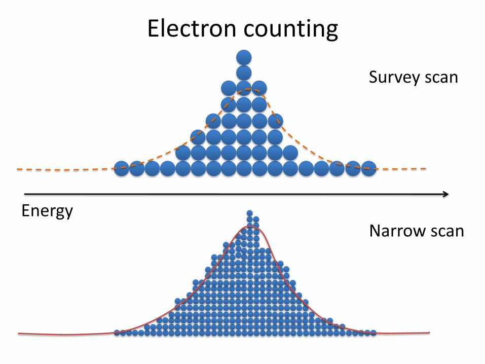
Electron counting

Energy

Survey scan

Narrow scan

Spot the Difference Find the 10 differences between the two pictures.

http://www.saizeriya.co.jp/entertainment/

This is what you might get.

93.4

93.5

93.6

93.7

93.8

93.9

94

94.1

94.2

94.3

0

50

100

150

200

0 50 100 150 200 250 300 350 400 450 500 550 600

Inte

nsi

ty n

orm

aliz

ed b

y Ip

(ar

b. u

nit

s)

Kinetic energy (eV)

What do you do next?

Co

un

ts p

er s

ec.

Photoelectron counts

I0 (p)

Ie

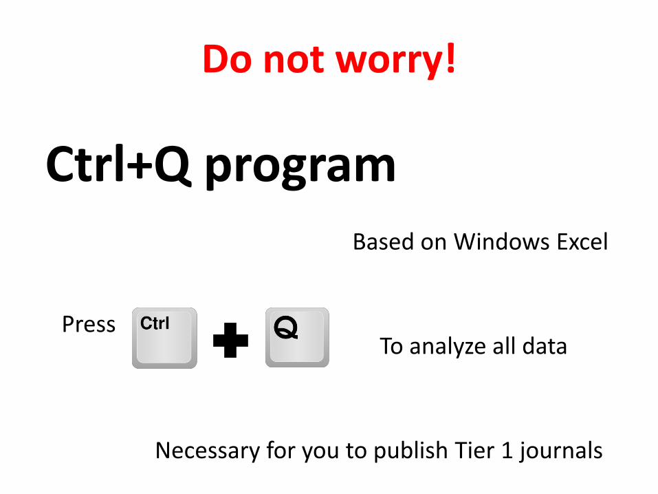
Do not worry!

Ctrl+Q program Based on Windows Excel

Press To analyze all data

Necessary for you to publish Tier 1 journals

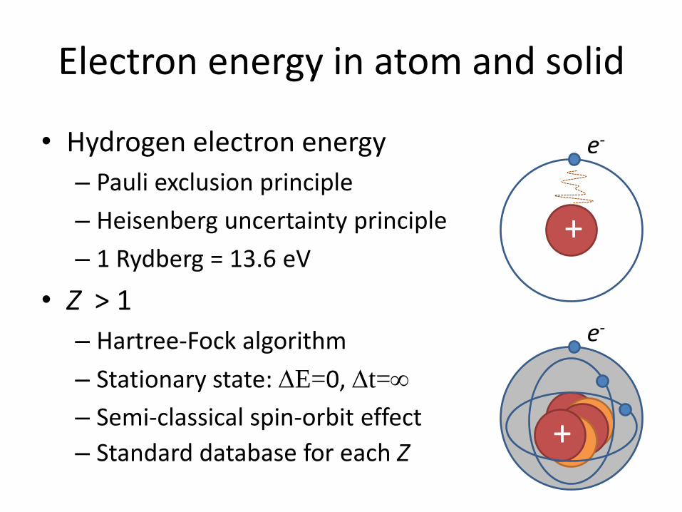
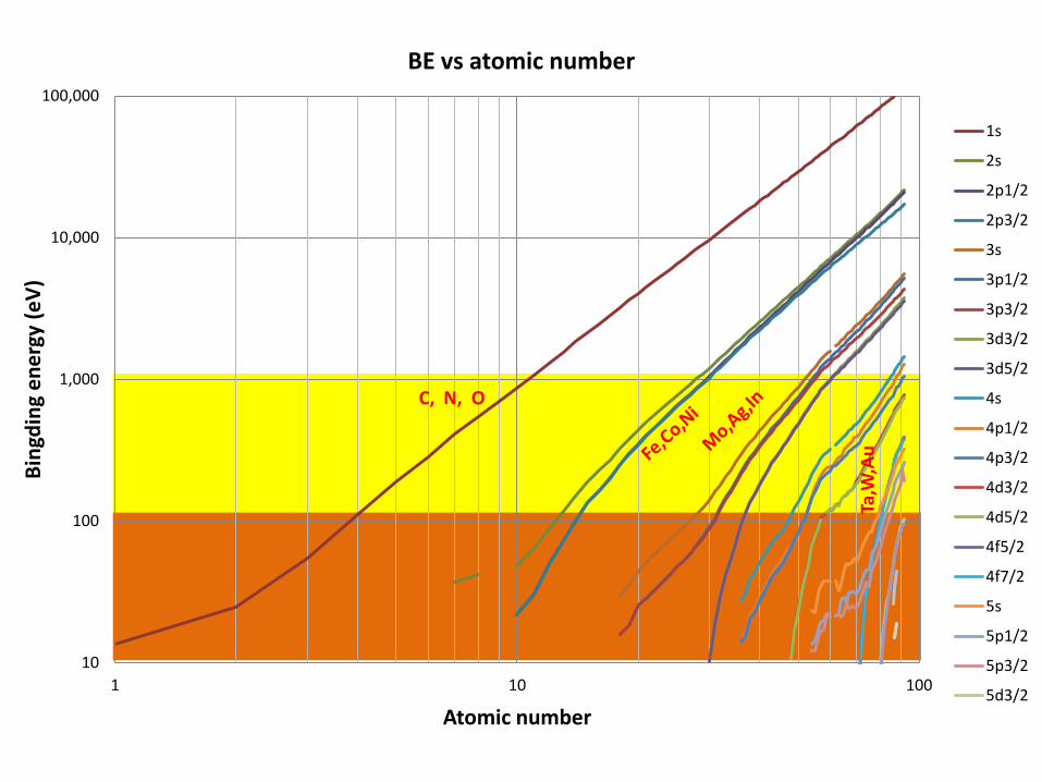
Electron energy in atom and solid

• Hydrogen electron energy

– Pauli exclusion principle

– Heisenberg uncertainty principle

– 1 Rydberg = 13.6 eV

• Z > 1

– Hartree-Fock algorithm

– Stationary state: DE=0, Dt=

– Semi-classical spin-orbit effect

– Standard database for each Z

+

e-

+

e-

+ +

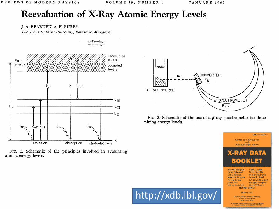
http://xdb.lbl.gov/

10

100

1,000

10,000

100,000

1 10 100

Bin

gdin

g e

ne

rgy

(eV

)

Atomic number

BE vs atomic number

1s

2s

2p1/2

2p3/2

3s

3p1/2

3p3/2

3d3/2

3d5/2

4s

4p1/2

4p3/2

4d3/2

4d5/2

4f5/2

4f7/2

5s

5p1/2

5p3/2

5d3/2

C, N, O

Ta,W

,Au

Spectral distributions

Delta function

Gaussian Lorentzian

Instrumental broadening Thermal (Doppler) broadening

Lifetime broadening Collision broadening

Voigt

FWHM 1/ (lifetime: )

Amplitude

FWHM

Amplitude 1/

energy 0 0 0

2

2

0

2exp

2

1

xxy 2

01

11

xxy

1

0,0

0,

dxx

x

xx

Light/electron optical ray-trace result in a probability distribution.

0 1 0

Slope

Offset

Peak de-convolution Background subtraction

Secondary electron background (inelastic scattering)

S/N √amplitude

Dark current

SE background

Auger/plasmon excitations

Collective electron excitations (plasmon)

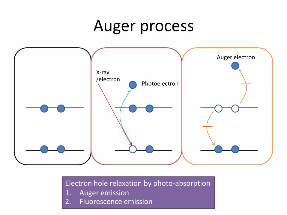
Auger process

Auger electron

Photoelectron

X-ray /electron

Electron hole relaxation by photo-absorption 1. Auger emission 2. Fluorescence emission

Spectrum Auger process Core excitation

/ionization

Auger yield(CFS) Valence band yield (ARPES)

Total electron yield

Kinetic energy

Core-level photoemission yield (CIS)

BEPES ≈ KEAES

# photons ≈ # electrons

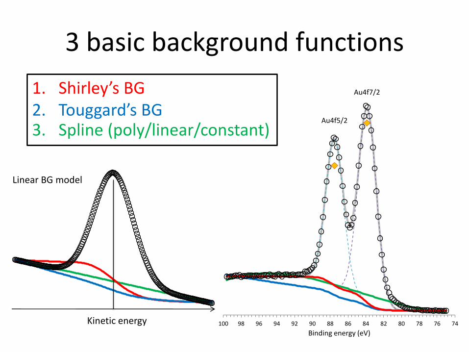
3 basic background functions

1. Shirley’s BG 2. Touggard’s BG 3. Spline (poly/linear/constant)

Au4f7/2

Au4f5/2

74 76 78 80 82 84 86 88 90 92 94 96 98 100

Binding energy (eV)

Linear BG model

Kinetic energy

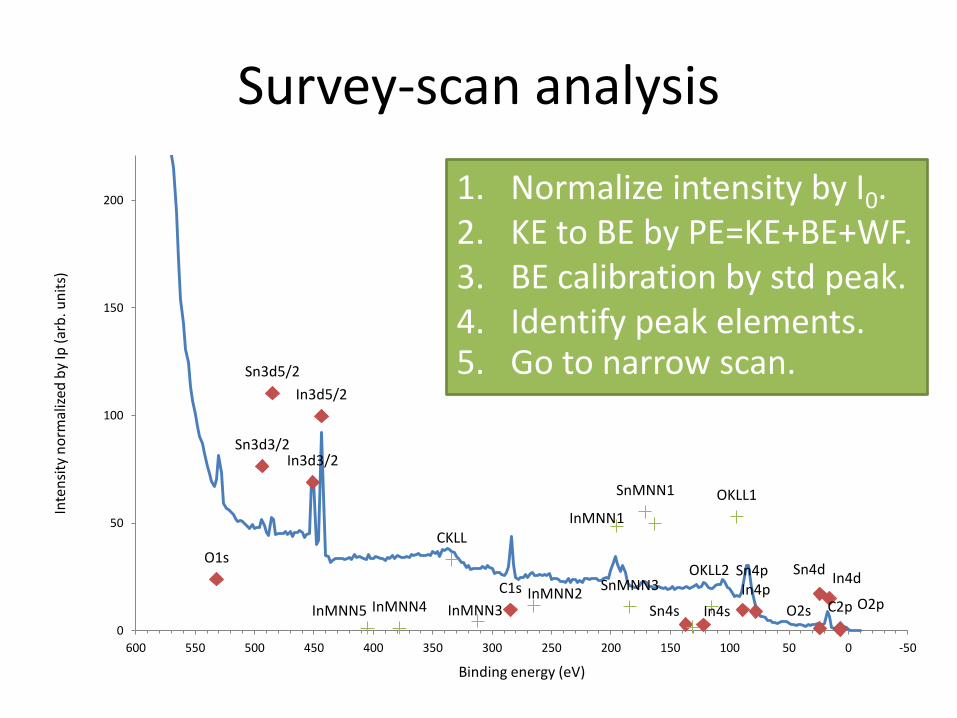
Survey-scan analysis

C1s C2p

O1s

O2s O2p

In3d3/2

In3d5/2

In4s

In4p In4d

Sn3d3/2

Sn3d5/2

Sn4s

Sn4p Sn4d

CKLL

OKLL1

OKLL2

InMNN1

InMNN2 InMNN3 InMNN4 InMNN5

SnMNN1

SnMNN3

0

50

100

150

200

-50 0 50 100 150 200 250 300 350 400 450 500 550 600

Inte

nsi

ty n

orm

aliz

ed b

y Ip

(ar

b. u

nit

s)

Binding energy (eV)

1. Normalize intensity by I0. 2. KE to BE by PE=KE+BE+WF. 3. BE calibration by std peak. 4. Identify peak elements. 5. Go to narrow scan.

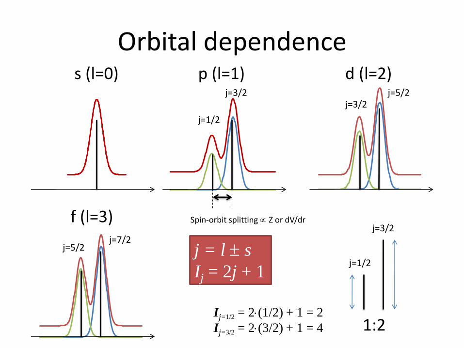
Orbital dependence p (l=1) s (l=0) d (l=2)

f (l=3)

j=1/2

j=3/2 j=3/2

j=5/2

j=5/2 j=7/2

Spin-orbit splitting Z or dV/dr

Ij=1/2 = 2(1/2) + 1 = 2

Ij=3/2 = 2(3/2) + 1 = 4 1:2

j=1/2

j=3/2

j = l s

Ij = 2j + 1

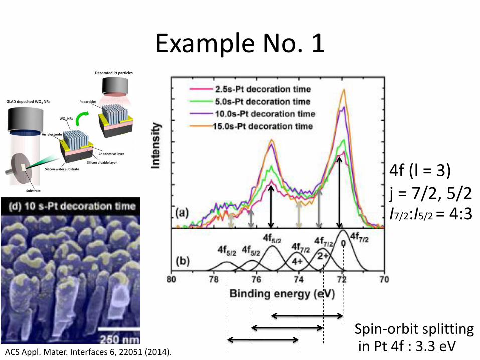
Example No. 1

ACS Appl. Mater. Interfaces 6, 22051 (2014).

4f (l = 3) j = 7/2, 5/2 I7/2:I5/2 = 4:3

Spin-orbit splitting in Pt 4f : 3.3 eV

Example No. 2

0

10

20

30

40

50

60

97 98 99 100 101 102 103 104 105 106 107

Inte

nsi

ty n

orm

aliz

ed b

y Ip

(ar

b. u

nit

s)

Binding energy (eV)

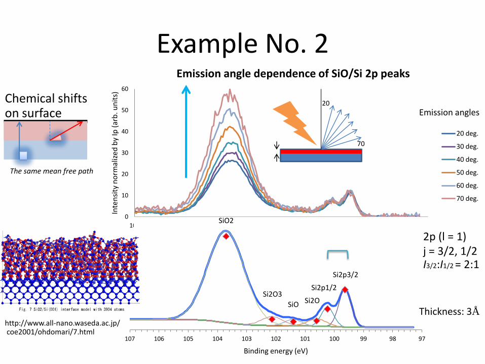
Emission angle dependence of SiO/Si 2p peaks

20 deg.

30 deg.

40 deg.

50 deg.

60 deg.

70 deg.

The same mean free path

Si2p3/2

Si2p1/2

Si2O SiO

Si2O3

SiO2

97 98 99 100 101 102 103 104 105 106 107

Binding energy (eV)

Emission angles

Thickness: 3Å

2p (l = 1) j = 3/2, 1/2 I3/2:I1/2 = 2:1

20

70

Chemical shifts on surface

http://www.all-nano.waseda.ac.jp/ coe2001/ohdomari/7.html

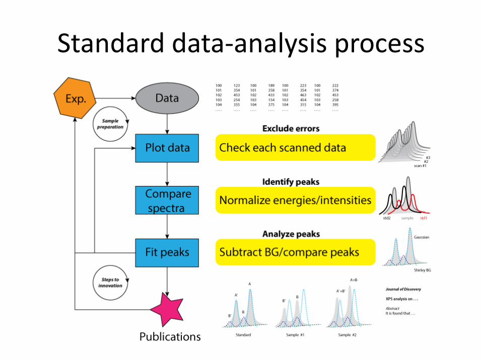
Standard data-analysis process

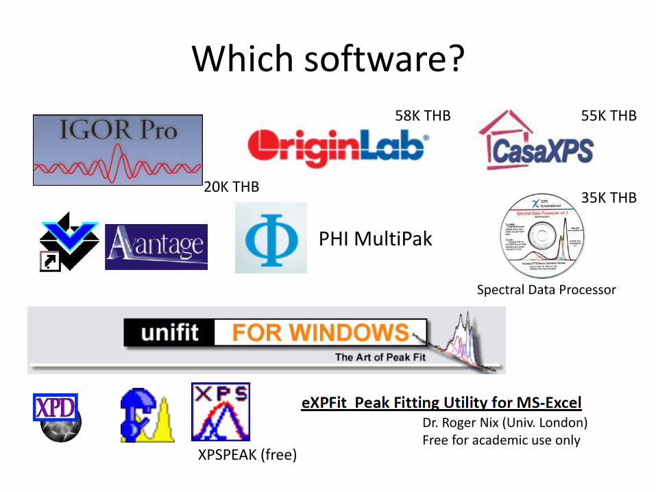
Which software?

PHI MultiPak

Spectral Data Processor

Dr. Roger Nix (Univ. London) Free for academic use only

XPSPEAK (free)

55K THB

35K THB

58K THB

20K THB

Which system you used?

Thermo CLAM2 NI LabVIEW

VG Scienta R4000 VG Scienta SES

PHI VersaProbe II PHI MultiPak

SUT-NANOTEC-SLRI

ULVAC-PHI MultiPak Licensed SLRI PC only Optimized for x-ray anode XPS machine

https://www.phi.com/surface-analysis-equipment/versaprobe.html

Wave Metrics Igor Pro

http://www.wavemetrics.com

595 USD (academic: 435 USD) It costs about 20,000 THB.

1. VG Scienta code • Load Spectrum • Reduce Dimension • Background … • Curve Fit … 2. Igor Pro XOP

Multi-peak Fit ver. 2

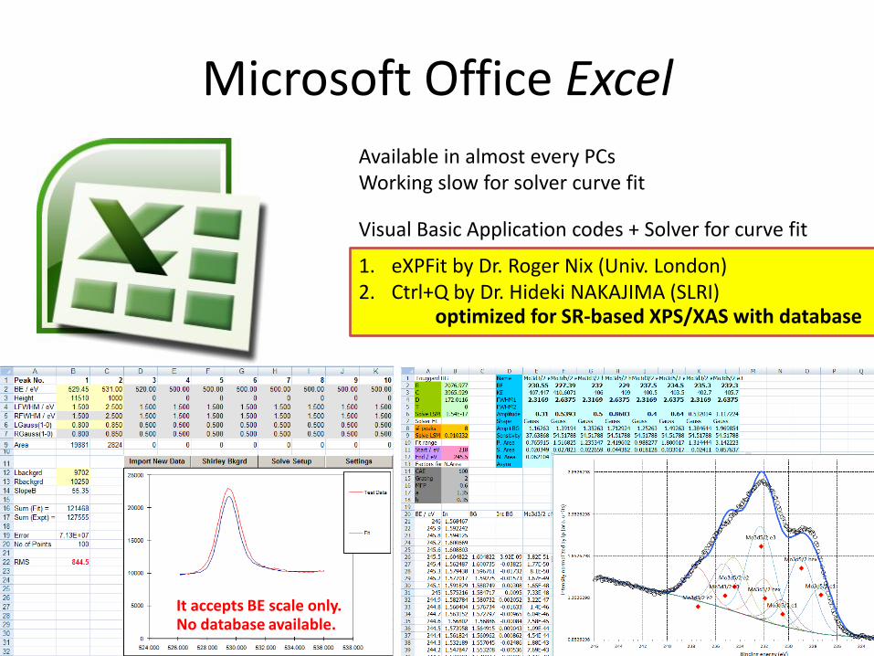
Microsoft Office Excel Available in almost every PCs Working slow for solver curve fit

Visual Basic Application codes + Solver for curve fit

1. eXPFit by Dr. Roger Nix (Univ. London) 2. Ctrl+Q by Dr. Hideki NAKAJIMA (SLRI)

optimized for SR-based XPS/XAS with database

It accepts BE scale only. No database available.

Over layer 50% transparent

http://www.saizeriya.co.jp/entertainment/

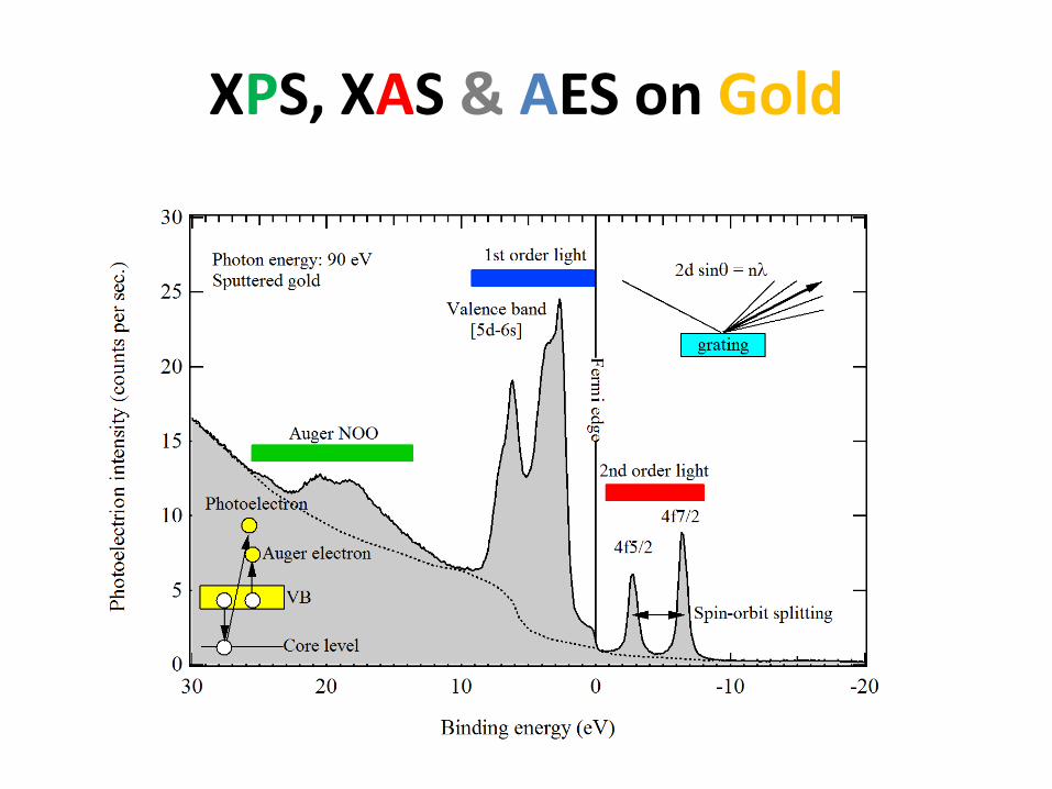
XPS, XAS & AES on Gold

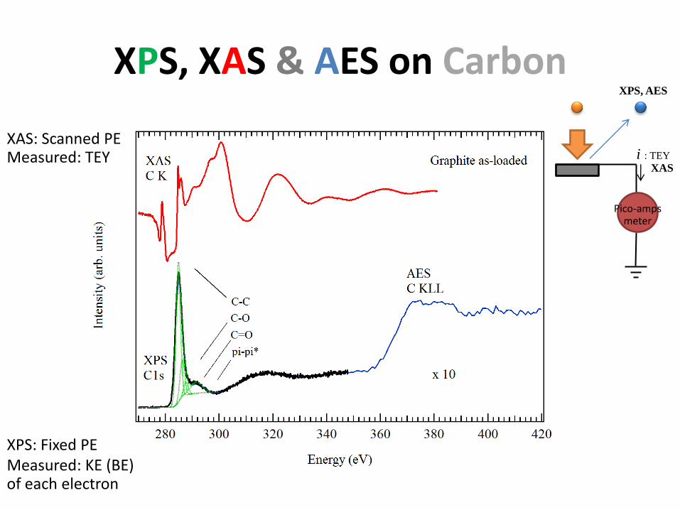
XPS, XAS & AES on Carbon

XAS: Scanned PE Measured: TEY

XPS: Fixed PE Measured: KE (BE) of each electron

Pico-amps meter

i : TEY

XPS, AES

XAS

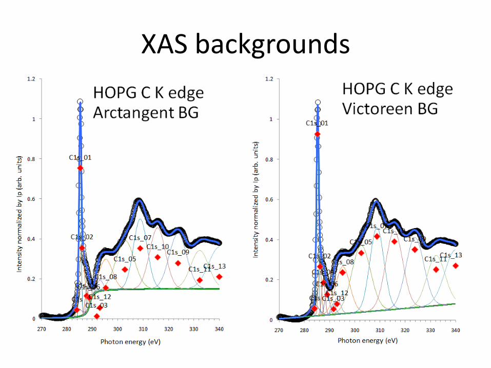
XAS backgrounds

Demonstrations

• Install Excel VBA code

– Igor Pro, Origin etc.

• Load data into Excel

• Check elements on spectra

• Calibrate energy at the reference

• Fit peaks to analyze the chemical shifts