Practice and Forgetting Effects on Vocabulary Memory: …act-r.psy.cmu.edu/wordpress/wp-content/uploads/2012/12/409s... · Practice and Forgetting Effects on Vocabulary Memory: An

Practice and Forgetting Effects on Vocabulary Memory:An Activation-Based Model of the Spacing Effect

Philip I. Pavlik Jr., John R. AndersonPsychology Department, Carnegie Mellon University

Received 4 September 2003; received in revised form 14 July 2004; accepted 17 November 2004

Abstract

An experiment was performed to investigate the effects of practice and spacing on retention of Japa-nese–English vocabulary paired associates. The relative benefit of spacing increased with increasedpractice and with longer retention intervals. Data were fitted with an activation-based memory model,which proposes that each time an item is practiced it receives an increment of strength but that these in-crements decay as a power function of time. The rate of decay for each presentation depended on the ac-tivation at the time of the presentation. This mechanism limits long-term benefits from further practiceat higher levels of activation and produces the spacing effect and its observed interactions with practiceand retention interval. The model was compared with another model of the spacing effect (Raaijmakers,2003) and was fit to some results from the literature on spacing and memory.

Keywords: Spacing effect; Distributed practice; Memory; Forgetting; Practice; Mathematicalmodeling

1. Introduction

Although practice and forgetting have been researched extensively by psychologists formore than 100 years (Ebbinghaus, 1885), there is still no consensus on the mechanisms re-sponsible for these effects. Central to finding this consensus is the need for explanations ofhow repetition improves recall, how increased temporal spacing of repetition improves recall,and how an increasing retention interval results in more forgetting.

Several theories exist. One major branch of theoretical explanation (Estes, 1955; Glenberg,1979; Raaijmakers, 2003) explains the effects of practice and forgetting largely as due to con-textual fluctuation. In this theory, each opportunity for practice results in an encoding of thestimulus and its context. However, the context of encoding fluctuates with the passage of time.Because of this fluctuation, as the spacing between repetitions increases, the overlap (redun-

Cognitive Science 29 (2005) 559–586Copyright © 2005 Cognitive Science Society, Inc. All rights reserved.

Requests for reprints should be sent to Philip Pavlik, Department of Psychology, Carnegie Mellon University,Pittsburgh, PA 15213. E-mail: [email protected]

dancy) of encoded contextual information decreases. This results in better memory perfor-mance as spacing becomes wider, because cue contextual information has a greater probabilityof matching the less redundant encoded information. Forgetting is also explained by contex-tual fluctuation theory because as retention intervals become longer the contextual informationpresent in a retrieval cue has fluctuated to become more dissimilar to the encoding context,thus decreasing recall ability. Recently, Raaijmakers developed an effective mathematicalmodel that realizes this type of theory. This article will take advantage of his work to comparethe contextual fluctuation approach to the theory we will develop here.

Although versions of the contextual fluctuation theory are consistent with much of the datain the literature, other theoretical accounts are possible. Specifically, another school of thought(Cuddy & Jacoby, 1982; Schmidt & Bjork, 1992; Whitten & Bjork, 1977) says that thelong-term memory strength contribution of a presentation depends on the accessibility of thememory at the time of the presentation. In this theory any repeated presentation that is moredifficult (e.g., due to an impoverished stimulus or long spacing interval) results in a greater im-provement in later recall ability due to this difficulty. Theories in this camp might loosely be re-ferred to as accessibility theories because the accessibility of a presentation controls thelong-run strength of the memory. One problem with these theories is that, in part because theyhave not been presented as fully specified formal models, it is unclear exactly how they wouldaddress all the effects in the literature.

As one instance of their lack of complete specification, accessibility theories have not madeclear the details of how they would explain the crossover interaction between retention intervaland spacing interval demonstrated by Bahrick (1979). Bahrick showed that when practice isspaced closely, it appears that forgetting occurs more quickly than when practice is spacedwidely. He had subjects practice Spanish–English paired associates for six practice sessionsseparated by 1, 7, or 30 days and looked at retention 30 days after the final session. He foundthat final recall was significantly better as spacing between practice sessions was increased,even though the performance during practice was significantly worse with wider spacing.

Contextual fluctuation theories and models can capture these crossover effects using the in-teraction of contextual fluctuation and the redundancy of encoded traces. If the retention inter-val is short, closely spaced practices will be remembered better than widely spaced practicesbecause the testing context will be similar to all the contexts of the closely spaced practices, butit will be similar to only the contexts of the most recent widely spaced practices. In contrast, ifthe retention interval is long, closely spaced practices will result in poorer recall because thetest context will have fluctuated away from the overlapping encoding contexts, whereas widelyspaced practices will result in better recall because the more diverse contextual information en-coded will be more likely to match the test context.

We became interested in the issue of the exact nature of the accumulation of recall strengthwith spaced practice because we noticed in some pilot work that the Adaptive Character ofThought–Rational (ACT–R) 5.0 declarative memory equations were not fitting the data well.Specifically, in an experiment in which we intermixed different spacings of practice we werefinding that we could not fit the data without supposing widely varying decay parameters foreach condition. Because this pilot experiment was not designed to adjudicate these issues, wedecided to design an experiment to address the issues of practice, forgetting, and spacing. Al-though verbal theories have provided interesting hypotheses of how these effects might occur,

560 P. I. Pavlik, J. R. Anderson/Cognitive Science 29 (2005)

we hoped to use the data from this experiment to make a formal model of these effects becausewe felt modeling was necessary to address the complexity of the issues involved.

The formal model we were seeking needed to specify both a practice function and a reten-tion function. Therefore, it is worthwhile reviewing the guidelines provided by Wickens(1999) for the necessary parts of a forgetting function, which can be generalized to practicefunctions. According to Wickens, these parts must include a representation for the initial learn-ing, a description of asymptotic performance, and a way to characterize changes in the rate offorgetting.

First, the initial learning represents the strength of a memory item at the beginning of a re-tention interval. This quantity reflects the impact of study in the period preceding the intervalrepresented in the forgetting function. From this initial level, memory strength decreases withtime as forgetting occurs. Second, the forgetting function needs to explain performance afterlong retention intervals as it approaches an asymptote. According to Wickens (1999), asymp-totic performance must be accounted for to explain results such as Bahrick (1984), which sug-gested that after about 3 years forgetting no longer occurs. Third, to characterize changes in therate of forgetting, Wickens suggested calculating a “hazard function,” which describes the rateof decrease of a memory at a particular time. He noted that the hazard function should agreewith Jost’s second law, which is essentially a statement that the rate of forgetting decreaseswith time: “If two associations are now of equal strength but of different ages, the older onewill lose strength more slowly with the further passage of time” (Woodworth, 1938).

Although Wickens (1999) limited his analysis to forgetting functions, these aspects of for-getting functions match to similar aspects of practice functions. Practice functions also need aninitial level, an asymptote, and a learning rate. However, unlike forgetting functions, whichpropose that forgetting is a continuous process, the learning rate in practice functions assumessome discrete increment for each added presentation. Therefore, our application of the learn-ing rate must be framed as a combination rule that adds up the effects of separate presentations.

Our model will capture these effects with a strength function that has built into it both thepower law of learning (a function of the number of practices) and the power law of forgetting (afunction of the retention interval). There has been much debate over whether power functionsare satisfactory for these purposes. Although some have argued that a power function charac-terizes practice data (e.g., Logan, 1992; Newell & Rosenbloom, 1981) and forgetting data(Wixted & Ebbesen, 1997), others have questioned whether a power function is satisfactoryand have suggested that exponential functions are more suitable for practice data (Heathcote,Brown, & Mewhort, 2000). It has also been proposed that practice functions may be a mixtureof multiple power functions (Delaney, Reder, Staszewski, & Ritter, 1998; Rickard, 1997). Stillothers have argued for the superiority of an exponential-power function in forgetting (Rubin &Wenzel, 1996; Wickelgren, 1974) and practice (Heathcote et al., 2000).

Our choice of a power function was based on analyses of how need probabilities for memo-ries fluctuate in the environment (J. R. Anderson & Schooler, 1991), yet it remains unclearwhy need probabilities for memories should follow power functions. Because it has beenshown that a mixture of exponential processes can produce power-law-like functions (R. B.Anderson & Tweney, 1997), one might speculate that a mixture of exponential decays in needprobability in the environment is the cause. Regardless, because biological processes often fol-low exponential decay functions, it is not difficult to suppose that forgetting matches power

P. I. Pavlik, J. R. Anderson/Cognitive Science 29 (2005) 561

functions in the environment because of a mixture of exponential processes in the brain. Essen-tially, the functional form we propose was chosen because it summarizes all the major effectsof relevance with a tolerable degree of error.

Our explanation of the integration of practice and forgetting began with this ACT–R mem-ory model (J. R. Anderson & Lebiere, 1998). This model specified how the exact pattern ofpractice and retention mapped to memory performance. However, it did not explain how thesefactors might interact with the spacing of practice. The model assumed that each presentationresults in an increment to memory, that these increments decay according to a power function,and that these decaying increments sum to yield an overall strength of the memory trace. Usingthis model, J. R. Anderson, Fincham, and Douglass (1999) reported success in fitting variouslatency data, but for this article, we modeled correctness of recall to facilitate comparisonswith other work.

To study practice and forgetting, we chose a paired-associate memory task in which partici-pants memorized the English translations of Japanese words. Foreign language vocabularylearning involves a basic memory task, but it still has external validity, and thus it seemed to bean ideal paradigm. Japanese was chosen to minimize the prior learning participants could bringto the task.

2. Experiment

2.1. Participants and design

Forty participants were recruited for this study from the Pittsburgh, Pennsylvania, commu-nity. They were mostly college students responding to an online advertisement. All partici-pants completed the experiment. Twenty participants each were assigned to the 1- and 7-dayretention conditions. Sessions lasted between 60 and 90 min. Only participants who professedno knowledge of Japanese were recruited.

In this experiment, participants learned the Japanese–English paired associates during afirst session (S1), and then 1 or 7 days later returned for a second session (S2) to assess their re-tention. During S1, participants learned the English responses for the Japanese cues over thecourse of 12 blocks of 40 presentations each. A presentation consisted of either a study trial ora test trial with feedback. The first 26 presentations of the first block were buffers and were notanalyzed. Following these buffers, the word pairs for each condition were introduced withstudy trials and then tested 1, 2, 4, or 8 times with 2, 14, or 98 intervening presentations. Thisindicates a 3 × 4 design (not including the two levels for the between-subject long-term reten-tion factor); however, because it would have made the experiment take too long, the 8 × 98 con-dition was not included, resulting in 11 within-subjects conditions. Each condition used eightword pairs. The introduction of pairs in each condition was distributed across the span of S1.Buffer items were used to fill in presentation spaces in the blocks that were not needed for the11 conditions.1

On S2, after a 1- or 7-day retention interval, the effects of these 11 conditions of trainingwere assessed with 11 blocks of 40 test trials. There were 27 buffer items to begin the first


block of S2. Following these buffers, all word pairs were retested four times each at a spacingof 98 presentations between retests.

2.2. Materials

The stimuli and buffers were 104 Japanese–English word pairs. English words were chosenfrom the MRC Psycholinguistic database such that the words had familiarity ratings between406 and 621, with a mean of 548, and had imagability ratings between 343 and 566, with amean of 464. These ratings were composed according to procedures described in the MedicalResearch Council (MRC) Psycholinguistic Database manual (Coltheart, 1981). The overallMRC database means for familiarity and imagability are 488 (SD 120) and 438 (SD 99) respec-tively, so the words we chose had higher familiarity and imagability ratings than the databaseaverages. Japanese translations (from the possible Japanese synonyms) were chosen to avoidsimilarity to common English words. Only four-letter English words were used, and four- toseven-letter Japanese translations were used. Japanese words were presented using Englishcharacters. Word assignment to conditions was randomized for each participant.

2.3. Procedure

Participants were instructed not to practice the word pairs during the time between sessions.Participants were scored for motivational purposes, receiving 6 points for each correct re-sponse and losing 12 points for each wrong response. Failing to provide a response, either bytime-out or by providing a blank response, resulted in a 0 score. Participants were paid $9 to$15 per session depending on their score.

The stimuli were shown on a 19-in. monitor at a resolution of 1,024 × 768 in 48-point whiteTahoma font on a blue screen. The stimuli pairs were centered vertically, the Japanese wordsappearing on the left and the English words on the right side of the screen. Participant promptsappeared centered horizontally, slightly above the words. Participant prompts were in 37-pointTahoma.

All trials were cued with the prompts “Study” or “Test” for 2 sec. Study opportunities al-lowed participants to view the new pair for 5 sec. Tests involved presentation of the Japaneseword on the left side of the screen. Participants typed the English translation on the right. If noresponse was made, the program timed out in 7 sec. Following response or failure to respond,the program displayed “Correct” or “Incorrect” for 1 sec and showed the change of score. If theresponse was correct, the next trial began. If incorrect, the word “Restudy” appeared for 2 sec,and there was a 5-sec restudy opportunity, identical with the original study trial.2

Between the blocks of 40 items, participants continued by pressing the space bar when theywere ready. Few participants paused at these opportunities. S2 procedures were identical, withrestudy trials after incorrect responses, but no new words were introduced.

The “recall or restudy” procedure for presentation of the stimuli was chosen based on the as-sumptions of the model we would be fitting to the data. According to this ACT–R memorymodel, study presentations and successful test presentations benefit memory equally. There-fore, our procedure results in one memory increment (according to the model) for each trial re-gardless of whether the participant responded correctly.


Although our model assumes each study or test counts equally, Carrier and Pashler (1992)noted in their literature review that studies and tests are not exactly equal. The identical creditwe give to test and study trials is essentially a simplifying assumption to reduce model com-plexity so the spacing effect model can be studied independently. Carrier and Pashler showedthe differences between studies and tests are not always large, so considering them equal is areasonable approximation for simplifying our model.

3. Results and discussion

By spacing the introduction of pairs across the session, S1 was designed to avoid confound-ing the conditions with serial position effects. Because of this, it did not seem that there shouldbe significant differences between correctness on the first two trials for items that were to re-ceive two practices, those that were to receive four, and those that were to receive eight, and in-deed there was none. This was shown through two repeated measures ANOVAs that were com-pleted to look for differences in the means of these first two trials across the different practiceconditions. To deal with the fact that the eight-repetition, 98-spacing condition was missingfrom a complete factorial design, we performed two analyses of variance (ANOVAs) on sub-sets of the design that were fully factorial. The first ANOVA was performed to compare themean percent correct on the first two presentations for two and four practice conditions (0.542and 0.515, respectively), averaged over 2, 14, and 98 spacing conditions. The difference wasnot significant, F(1, 39) = 3.1, p > .05. The second ANOVA was performed to look at the meansfor two, four, and eight practices (0.662, 0.643, and 0.653, respectively) aggregated for 2 and14 spacing. There were no significant differences, F(2, 38) = 0.60, p > .05. We also looked forserial position effects within conditions. The eight items of each condition were introduced insequence across the experiment, so we looked at the first test trials of all items and found aver-ages of correctness for these first trials by their order of introduction. This gave eight meansspread fairly evenly across the experiment. An ANOVA looking for differences in these meansfound nothing significant, F(7, 273) = 1.925, p > .05.

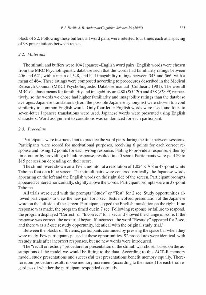
Because of the similarity across practice conditions, S1 data were aggregated for display(see Fig. 1). To confirm that performance improved across this first session and to look for ef-fects of the spacing manipulation during S1, a repeated measures ANOVA (first four trials ofS1 aggregated by Practice condition × S1 spacing × S2 retention interval group) was com-pleted. The results of this analysis confirmed that performance improved across the first fourtrials of S1, F(3, 114) = 412, p < .001, and that there was significantly lower performance withwider spacing, F(2, 76) = 240, p < .001. The lower performance on S1 with wider spacing waslikely due to the overall longer retention intervals for these trials. The difference in S1 learningfor the 1- and 7-day retention groups was not significant on S1, F(1, 38) = 1.13, p = .296.

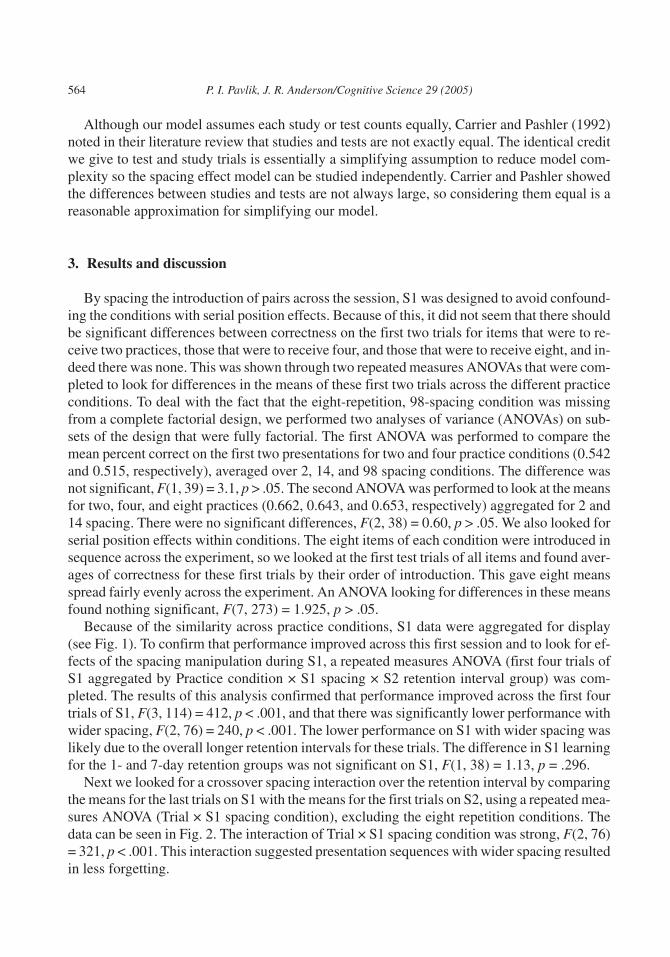
Next we looked for a crossover spacing interaction over the retention interval by comparingthe means for the last trials on S1 with the means for the first trials on S2, using a repeated mea-sures ANOVA (Trial × S1 spacing condition), excluding the eight repetition conditions. Thedata can be seen in Fig. 2. The interaction of Trial × S1 spacing condition was strong, F(2, 76)= 321, p < .001. This interaction suggested presentation sequences with wider spacing resultedin less forgetting.



Fig. 1. Experiment S1 aggregate data for humans and model for spacing conditions. 2 SE confidence intervals com-puted from participant means.

Fig. 2. Spacing Crossover Interaction. S2 initial trial performance and S1 final trial performance as a function ofspacing. Values exclude the 8 test trial condition and aggregate all other repetition and retention conditions. 2 SEconfidence intervals computed from participant means.

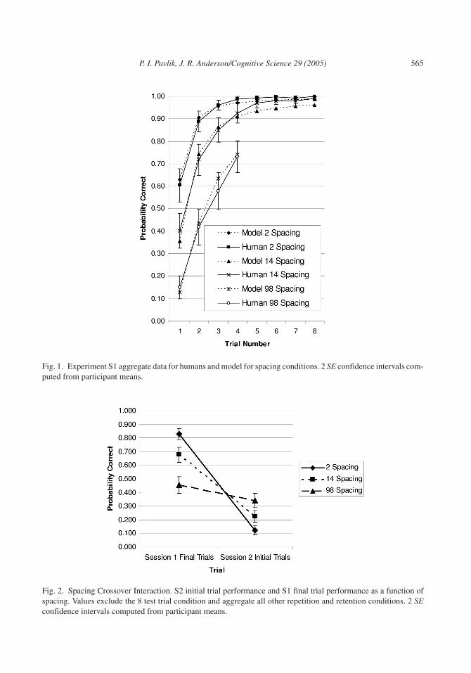
We were then interested in showing the effects present in the S2 data. The mean correctnessfor S2 was 0.64 for the 1-day retention interval and 0.52 for the 7-day retention interval. Be-cause the patterns of data were similar between the two retention intervals on S2 (r = .959, p <.001), we aggregated the two conditions for purposes of display (see Fig. 3). Some main effectsand interactions can be noted. A repeated measures ANOVA of S2 data (S1 repetitions × S1spacing × S2 trial × Retention interval, excluding the eight repetition conditions due to the in-


Fig. 3. Experiment 1 S2 aggregate data for humans and model for practice conditions by spacing intervals. Individ-ual graphs for each repetition condition. 2 SE confidence intervals computed from participant means.

complete design) was completed. First, this analysis showed that people forgot more when theretention interval went from 1 to 7 days, F(1, 38) = 4.26, p < .05. It also revealed a strong maineffect of spacing, F(2, 76) = 58.2, p < .001. More important, we found a significant S1 repeti-tion × S1 spacing interaction, F(4, 152) = 4.38, p < .005, reflecting an increasing benefit tospacing with more repetitions at a particular spacing. This is similar to interactions producedby Underwood (1969). As can be seen from Fig. 3, there was a dramatic increase in the impor-tance of spacing as S1 repetitions increased.

4. Discussion of model and theory

Our modeling of these data was motivated by the experiment and by results such as Bahrick(1979). Notable in such results are strong crossover interactions. Crossover interactions suchas Bahrick’s and our interactions (see Fig. 2) suggest that the rate of forgetting is different de-pending on the spacing of practice. Although statistical analysis of this sort of forgetting-rateinteraction are notoriously difficult due to scaling issues (Bogartz, 1990), the crossovers wefound would occur regardless of scaling and thus were good evidence that in our experimentforgetting was slower after a series of spaced presentations in comparison to a more massedseries.

Another result of interest was the finding that the effects of spacing are greater the morepractice trials there are. Combined with the crossover interactions, it implied that the benefitsof spacing in slowing the forgetting rate become larger as the number of practice trials in-creases.

To model these data we needed a formal system that (1) predicted the improvement in per-formance that occurs with practice, (2) predicted the decrease in performance with delay, (3)predicted the spacing effect, (4) predicted the interaction of spacing with retention (that spacedpractice shows greater advantage with greater delay), and (5) predicted the interaction of spac-ing with practice (that spacing is more important when there are more practice trials). The stan-dard ACT–R model seems well suited to handle the effects of practice and the effects of reten-tion interval. It not only predicts the effects of practice but also the form of the practice andretention functions—that they are both roughly power functions. We review how the theorypredicted these effects first, before going on to describe the elaboration that we produced to in-clude the spacing effect and its interactions with practice and retention.

ACT–R’s activation equation represents the strength of a memory item as the sum of a num-ber of individual memory strengthenings, each corresponding to a past practice event. It pro-poses that each time an item is practiced the activation of the item receives an increment instrength that decays away as a power function of time. These individual strengthenings3 re-sulted in the following equation for strength of an item after n presentations:

In this function, m is the activation of the item as a function of the times (tis) since each of then prior presentations.4 Each ti is how long ago the ith practice of that item occurred, and these


1

1

( ) (1)n

dn n i

i

m t ln t �

�

� ��

values are scaled to account for differences in interference (this scaling is detailed later). Thedecay parameter (d) is a constant. Combined with the response functions in ACT–R, this acti-vation equation produces the power laws of practice and forgetting. One can note regardingWickens (1999) that this equation provides a number of the required components of practiceand forgetting functions. It defines initial learning given prior practice, and it explains both theprogression of forgetting and the integration of the effect of each discrete practice event.

Because ACT–R is a complex system, for this article we model simply the effect of practiceand forgetting on a trace that encodes the two items in a paired associate. Further, our modelabstracts over issues of cuing and context. In the full ACT–R model, in addition to any effectsof practice and forgetting on the memory of the trace encoding the paired associate, spreadingactivation from the number of cues or from the context affects the activation of a memory.However, because the effect of number of cues and context is constant across trials in our ex-perimental task (because there is only one cue and our context does not fluctuate with time),the predictions we make are equivalent to those from the full activation equation. Given this ex-periment, if we were to consider the spreading activation term, we would simply need toreestimate τ (in the following equation) to compensate for the constant increase due to activa-tion spread.

The response function of interest in this experiment concerned accuracy. In ACT–R, an itemwill be retrieved if its activation is above a threshold. Because activation is noisy, an item withactivation m as given by Equation 1 has only a certain probability of recall. ACT–R assumes alogistic distribution of activation noise, in which case the probability of recall is:

In this equation, τ is the threshold parameter and s is the measure of noise. An inspection ofthe formula shows that, as m tends higher, the probability of recall (pr) approaches 1, whereas,as τ tends higher, the probability decreases. In fact, wheν τ = m, the probability of recall is .5.The s parameter controls the noise in activation, and it describes the sensitivity of recall tochanges in activation. If s is close to 0, the transition from near 0% recall to near 100% will beabrupt, whereas when s is larger, the transition will be a slower sigmoidal curve. Because thisfunction results in diminishing marginal returns for practice and diminishing marginal lossesfor forgetting, it address the need for explaining asymptotic performance described byWickens (1999).

Although the recall probability function explains one aspect of asymptotic forgetting, theslowdown of forgetting over long delays between practice sessions, exemplified by our experi-ment, is handled by a scaling of the ti values in Equation 1. J. R. Anderson et al. (1999) foundthat although the activation equation could account for practice and forgetting effects within anexperiment, it was not able to fit retention data over long intervals between sessions (theylooked at retention intervals of up to 1 year). Therefore, they found it necessary to suppose thatbetween sessions there is less destructive interference from intervening memory events thanduring an experimental session. They modeled the apparent slowing of decay by scaling thepassage of time outside the experiment. Forgetting is then dependent on this “psychological


1( ) (2)

1r m

s

p m

eτ�

�

time” between presentations rather than the real time. This is implemented by multiplying theportion of time that occurred between sessions by the h parameter.5

In this theory, then, interference interacts with the decay rate to control the true rate of for-getting. For the models in this article, the scale factor to convert real time to psychological time(a measure of intervening interfering events) is 1 within an experiment and 0.025 between ex-periments. Therefore, in our memory equations, each ti represents the cumulative interferencea presentation has encountered. Because of this the rate of memory loss for any ti

–d at any time(the hazard rate) is best thought of as being a function of the decay rate and the total amount ofinterference encountered. Thus, we are supposing that Jost’s law applies to interference andmight be restated as follows: Given two memories, both of which are currently equal in recallstrength, the one that has already suffered the most from interference will be forgotten moreslowly.

This intuition from the model allows the theory to provide a bridge between understandingforgetting in terms of time and understanding forgetting in terms of interference. Forgetting inthis theory is linked to time, but it also depends on the rate of interference for an interval. Be-cause we have found that h (the interference rate) tends to be stable, we have used the same ra-tio 1/40 (interference being 40 times greater within an experiment) across the two experimentswe fit that have between-session intervals. We would have been able to fit the data for these ex-periments more tightly if we had estimated different h values for each experiment, or if we hadnot assumed within-experiment h to be 1 (as we do for all our fits), but conceptually it wouldhave been more difficult to interpret differences in forgetting due to spacing. Because we arefocusing on spacing effects more than interference processes here, we decided to forgo investi-gation of how h might vary for each experiment.

4.1. Decay rate as a function of activation

Even with the elaboration offered by J. R. Anderson et al. (1999), ACT–R (J. R. Anderson &Lebiere, 1998) was incapable of predicting any crossover spacing effect. However, J. R. An-derson and Schooler (1991) proposed a modification to the ACT–R strength equation that doescapture the spacing effect. This modification specified that each presentation had an individualdecay rate that depended on the spacing from the prior presentation. It was a formalization of amechanism suggested by Wickelgren (1973). J. R. Anderson and Schooler’s specific proposalwas that the ith presentation would have the decay rate:

di(ti, ti–1) = max[d, b(ti – ti–1)–d] (3)

InEquation3,d is theminimumdecayrate (whichapplies for the firstpresentationandforpre-sentations at long enough lags.) At shorter lags the decay rate for a presentation is itself a powerfunction of the lag, ti – ti–1. Although J. R. Anderson and Schooler (1991) had some success withthis form of the equation they commented that “its exact form is a bit arbitrary” and that “there isnot evidence one way or the other for this precise” formulation (p. 407). We had at least threeother problems. First, it made the decay rate for a presentation just a function of the lag since thelast item,and thisdidnot seemtobeplausible.Second,ournewformulationprovidedmarginallybetter fits across models. Third, we have found the new formulation has more parameter stabilityacross models. This final point suggests it may better describe the underlying processes.


As an alternative to the J. R. Anderson and Schooler (1991) proposal, we developed anequation in which decay for the ith presentation (considering the initial study as Presentation1), di, is a function of the activation at the time it occurs instead of at the lag (see Equation 4.)This implies that higher activation at the time of a trial will result in the gains from that trial de-caying more quickly. On the other hand, if activation is low, decay will proceed more slowly.Specifically, we propose Equation 4 to specify how the decay rate, di, is calculated for the ithpresentation of an item as a function of the activation mi–1 at the time the presentation occurred.Equation 5 then shows how the activation mn after n presentations depends on the decay rates,dis, for the past trials.

In Equation 4, c is the decay scale parameter, and a is the intercept of the decay function.6

For the first practice of any sequence, d1 = a because m0 is equal to negative infinity. Note thatwhen c = 0, Equation 4 is nullified, and Equation 5 collapses to the standard ACT–R Equation1. These equations are recursive because to calculate any particular mn one must have previ-ously calculated all prior mns to calculate the dis needed. The Appendix includes a detailed ex-ample applying these equations for a sequence of five presentations. These equations result in asteady decrease in the long-run retention benefit for additional presentations in a sequence ofclosely spaced presentations. As spacing gets wider in such a sequence, activation has time todecrease between presentations; decay is then lower for new presentations, and long-run ef-fects do not decrease as much.

The original ACT–R model (Equation 1) does not produce the spacing effect because it hasno mechanism to reflect that time differences between practices should matter much. Thespacing effect in this model (Equations 4 and 5) occurs because when spacing between twopresentations is wider, the decay rate for the second presentation is lower. At long retention de-lays, this more than compensates for the fact the first presentation suffers more forgetting dueto the increased retention interval from the wider spacing.

The new model shows that each practice contributes to a single unitary strength measure forthe represented chunk. However, the activation equation captures this overall strength as anumber of discrete contributions represented explicitly by the contribution from each t i

di� . Aneural analogy for this relation might suppose that each experience (ti) results in the creation ofnew receptor sites at the synapses that correspond to the overall memory trace. Indeed, an addi-tion of synapses with the induction of long-term potentiation (LTP) of neural connections hasbeen shown experimentally. For instance, Toni et al. (2001) and Geinisman (2000) showed thatLTP induction results in perforated areas on dendritic spines, which later develop intomultisynapse connections with presynaptic cells. Presynaptic cells undergo a similar activ-ity-dependent remodeling that results in new axonal synapses (Nikonenko, Jourdain, & Mul-ler, 2003).

The model then says that the stability of these new receptor sites (we can consider the –di

value as a measure of stability) is less when they are created when strength is already high. In


11( ) (4)imi id m ce a��

1

1

( ) (5)in

dn n i

i

m t ln t �

�

� ��

general, this argument supposes that the faster forgetting following massed practice may re-flect diminishing marginal returns in the initiation of the neural consolidation processes.7 In-deed, one can see that decay and consolidation are analogous in the theory because the di pa-rameter can characterize either depending on its sign. Like decay, consolidation can beconsidered a continuous process that is initiated at encoding and involves memories becomingmore stable over time (in conformance with Jost’s law), but they are simultaneously degradingdue to forgetting processes.

We attempted to fit a model using Equations 2, 4, and 5 to the data from the experiment. Allfits for this article were performed by minimizing a χ2 statistic computed from the conditionmeans according to the formula

Where the summation is over the i data points, Ni is the number of observations for each datapoint, predi is the predicted recall probability in condition i, and obsi is the observed probabil-ity. We should note that this statistic does not satisfy the assumptions of the chi-square distribu-tion because of nonindependence of observations. However, minimizing it is still a reasonableway to estimate parameters, and its use allows comparison with Raaijmakers (2003), who usedthis statistic in the same way. As an alternative to evaluate and compare fits we have also pro-vided r2 and root mean square deviation (RMSD) statistics. In this article, the RMSD valueswere adjusted for model complexity by subtracting the number of parameters from the divisorwhen computing the mean, as described in Pitt, Myung, and Zhang (2002).

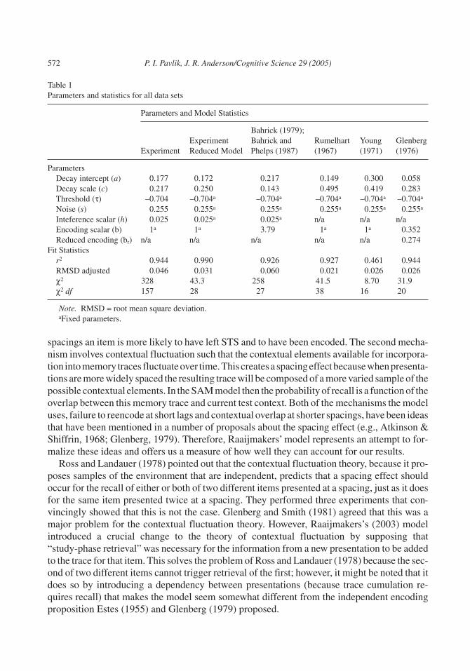
We applied this extended ACT–R model to the experiment to fix parameters, which we triedto preserve in fitting other data sets. For this experiment, there were 162 aggregate correctnessaverages (the obsis in the previously mentioned chi-squared summation) to be fitted and splitinto 81 points for each between-subject retention interval, of which 37 points were for the S1conditions, and 44 points were for the S2 conditions. Table 1 gives the parameters and good-ness-of-fit measures for this model. As is apparent from Figs. 1 and 3, the model mirrored theabsolute and relative patterns in the data closely.

Applying the model to the experiment allowed us to fix default parameters for the model.Using these defaults, we then adopted the policy of keeping as many parameters as constant aspossible between models. Because this policy limits the complexity of our model, we believe itimproves its explanatory utility.

4.2. ACT–R versus contextual fluctuation (SAM)

Raaijmakers (2003) extended the search of associative memory (SAM) model (Raaijmakers& Shiffrin, 1981) to account for the spacing effect and successfully fit the model to some datasets.Therefore,wedecided tocompareRaaijmakers’modelwithoursusing thedata fromourex-periment and three experiments that Raaijmakers reported fits to. His model has two mecha-nisms that cause spacing effects. First, it has a short-term store (STS) mechanism that containsrecently encoded information. If an item is still in this STS at the time of a later presentation, thenew presentation does not get a second encoding. This creates a spacing effect because at longer


22

2

( )(6)i i i

i ii

N pred obs

pred predχ �

��

spacings an item is more likely to have left STS and to have been encoded. The second mecha-nism involves contextual fluctuation such that the contextual elements available for incorpora-tion intomemory traces fluctuateover time.Thiscreatesa spacingeffectbecausewhenpresenta-tions are more widely spaced the resulting trace will be composed of a more varied sample of thepossible contextual elements. In the SAM model then the probability of recall is a function of theoverlap between this memory trace and current test context. Both of the mechanisms the modeluses, failure to reencode at short lags and contextual overlap at shorter spacings, have been ideasthat have been mentioned in a number of proposals about the spacing effect (e.g., Atkinson &Shiffrin, 1968; Glenberg, 1979). Therefore, Raaijmakers’ model represents an attempt to for-malize these ideas and offers us a measure of how well they can account for our results.

Ross and Landauer (1978) pointed out that the contextual fluctuation theory, because it pro-poses samples of the environment that are independent, predicts that a spacing effect shouldoccur for the recall of either or both of two different items presented at a spacing, just as it doesfor the same item presented twice at a spacing. They performed three experiments that con-vincingly showed that this is not the case. Glenberg and Smith (1981) agreed that this was amajor problem for the contextual fluctuation theory. However, Raaijmakers’s (2003) modelintroduced a crucial change to the theory of contextual fluctuation by supposing that“study-phase retrieval” was necessary for the information from a new presentation to be addedto the trace for that item. This solves the problem of Ross and Landauer (1978) because the sec-ond of two different items cannot trigger retrieval of the first; however, it might be noted that itdoes so by introducing a dependency between presentations (because trace cumulation re-quires recall) that makes the model seem somewhat different from the independent encodingproposition Estes (1955) and Glenberg (1979) proposed.


Table 1Parameters and statistics for all data sets

Parameters and Model Statistics

ExperimentExperimentReduced Model

Bahrick (1979);Bahrick andPhelps (1987)

Rumelhart(1967)

Young(1971)

Glenberg(1976)

ParametersDecay intercept (a) 0.177 0.172 0.217 0.149 0.300 0.058Decay scale (c) 0.217 0.250 0.143 0.495 0.419 0.283Threshold (τ) –0.704 –0.704a –0.704a –0.704a –0.704a –0.704a

Noise (s) 0.255 0.255a 0.255a 0.255a 0.255a 0.255a

Inteference scalar (h) 0.025 0.025a 0.025a n/a n/a n/aEncoding scalar (b) 1a 1a 3.79 1a 1a 0.352Reduced encoding (br) n/a n/a n/a n/a n/a 0.274

Fit Statisticsr2 0.944 0.990 0.926 0.927 0.461 0.944RMSD adjusted 0.046 0.031 0.060 0.021 0.026 0.026χ2 328 43.3 258 41.5 8.70 31.9χ2 df 157 28 27 38 16 20

Note. RMSD = root mean square deviation.aFixed parameters.

To enable this model to handle long-term memory data from our experiment we added amechanism like the “psychological time” mechanism in our model. This allowed the model afree parameter to find the best fitting number of trials to represent the forgetting over the timebetween sessions. With this adjustment it was possible to take the model that Raaijmakers(2003) developed for a model of Rumelhart’s (1967) data, adjust it to reflect the presentationschedule in our experiment, estimate new parameters, and make predictions. However, we en-countered a couple of difficulties in fitting the Raaijmakers model to our data.

The first issue was purely technical. Because of the combinatorial complexity of theRaaijmakers model, it was impractical to model the eight-test trial condition. Therefore, weexcluded these data from our modeling effort. To further limit the combinatorial complexity,we only looked at first trial performance on S2. The second issue was more complex. The basicRaaijmakers model was simply unable to fit the S1 learning data in the 98-spacing condition.This is largely because retrieval during practice is so poor with 98 spacing that the tracecumulation mechanism fails to result in the memory gains observed. Because including thiscondition in the Raaijmakers model seriously distorted the parameter estimation, and still re-sulted in poor fits, we altered the model slightly at Raaijmakers suggestion (personal commu-nication, March 8, 2004), so the study-phase retrieval mechanism occurred automatically. Thismade it so that the repetitions were always recognized and trace cumulation could not fail.

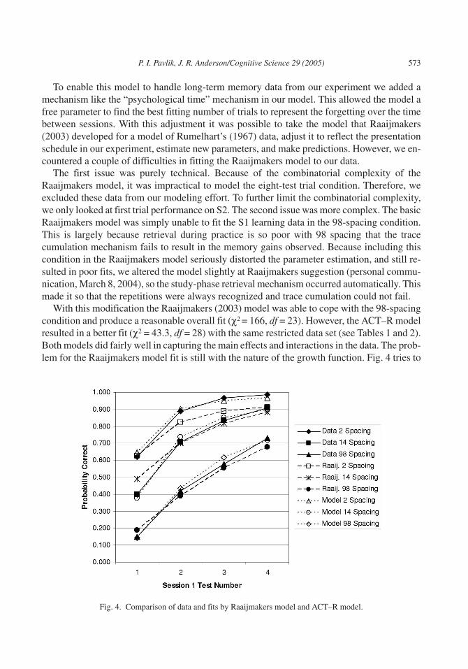
With this modification the Raaijmakers (2003) model was able to cope with the 98-spacingcondition and produce a reasonable overall fit (χ2 = 166, df = 23). However, the ACT–R modelresulted in a better fit (χ2 = 43.3, df = 28) with the same restricted data set (see Tables 1 and 2).Both models did fairly well in capturing the main effects and interactions in the data. The prob-lem for the Raaijmakers model fit is still with the nature of the growth function. Fig. 4 tries to


Fig. 4. Comparison of data and fits by Raaijmakers model and ACT–R model.

show what is behind the lack of fit of the Raaijmakers model. (The complete Raaijmakersmodel fit is available at the Web site.1) In Fig. 4, we have averaged over the 1, 2, and 4 practiceconditions to look at the forms of the learning curves. One can note that the Raaijmaker’smodel has a problem with capturing sufficient Final Session 1 learning across all the condi-tions. In part, particularly for the two-spacing condition, this may be caused by the STS mecha-nism blocking encoding when an item remains in STS on repetition. Because of this mecha-nism, closely spaced practices do not gain much contextual strength because of overlap andbecause they are sometimes not encoded. It appears that the model cannot compensate for thisby adjusting the contextual overlap parameters, likely because this would upset the fit of the98-spacing condition in which the STS mechanism plays no role. To check the possibility thatthis problem was due to issues involving the fit to Session 2 tests, we also ran the model foronly Session 1 data; this did not greatly improve the fit to the learning curves (χ2 = 104,df = 14).

Later in this article, we present comparisons of our model fits with the Raaijmakers (2003)model fits for a set of three experiments in the literature. Our model fits these data sets compa-rably well and with fewer parameters. It seems reasonable to infer that the Raaijmakers modeland the ideas on which it is based can predict many of the basic effects of spacing, as our modelcan. However, the following experiments did not measure retrieval performance over as large arange of correctness values as our experiment did, and therefore this issue with the learningfunction was not noticed. Thus, our current experiment brought out a critical advantage of ourmodel in capturing the learning curves during spaced practice.

5. Other model fits

To test further the generalizability of our model, we fit it to four examples from the memoryliterature. For each of these fits we varied as few parameters as possible, preferring instead touse the defaults from the experiment. The first experiment involved long-term retention inter-vals, whereas the following three experiments involved only a single session. These three sin-gle-session experiments were also modeled by Raaijmakers (2003), and we briefly compareour fits of these experiments with his fits.

5.1. Bahrick

Bahrick’s (Bahrick, 1979; Bahrick & Phelps, 1987) results on learning Spanish–English vo-cabulary pairs are seminal in discussions of the spacing effect, and therefore we wanted toshow that our model could account for them. In Bahrick, participants memorized 50 Span-ish–English vocabulary pairs. The training took place over three or six sessions. Each sessionbegan with testing of all the words followed by a presentation sequence of any word pairs notrecalled. After presentation, these words were retested and the procedure repeated until allwords were correctly recalled once in each session. The experimental sessions were spaced ev-ery 0, 1, or 30 days and were followed by a final test session at a 30-day retention interval. Ta-ble 2 shows the performance during the initial testing sequence of each session. The first train-ing session did not begin with testing, and thus it is not listed. We have also included the data


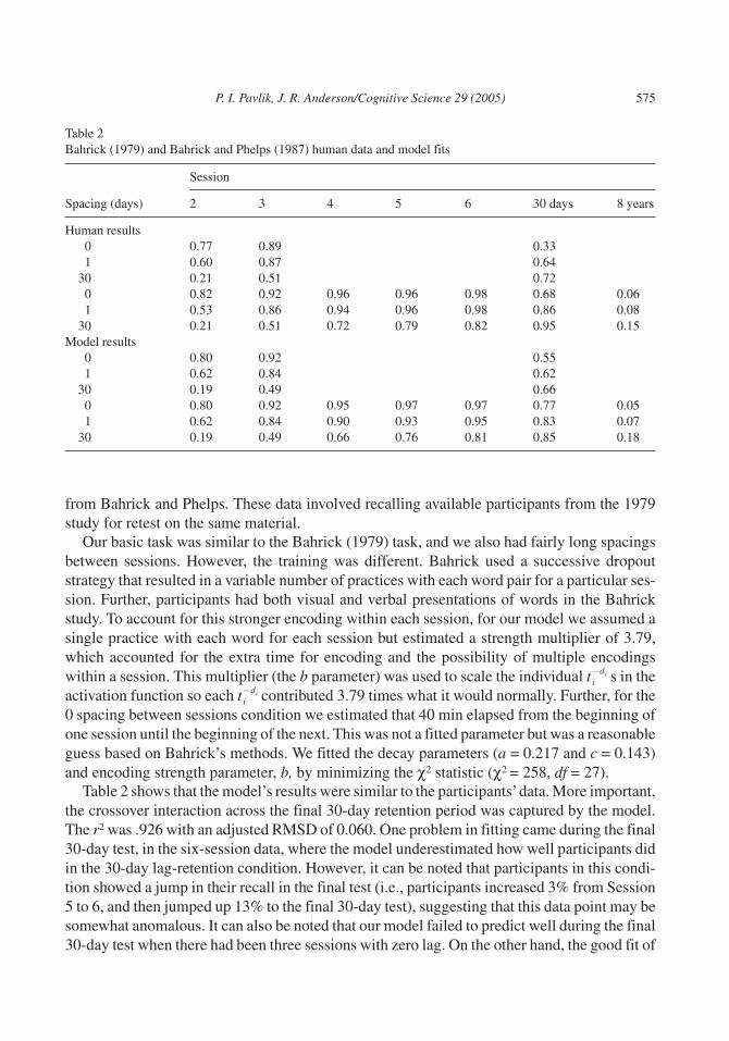
from Bahrick and Phelps. These data involved recalling available participants from the 1979study for retest on the same material.

Our basic task was similar to the Bahrick (1979) task, and we also had fairly long spacingsbetween sessions. However, the training was different. Bahrick used a successive dropoutstrategy that resulted in a variable number of practices with each word pair for a particular ses-sion. Further, participants had both visual and verbal presentations of words in the Bahrickstudy. To account for this stronger encoding within each session, for our model we assumed asingle practice with each word for each session but estimated a strength multiplier of 3.79,which accounted for the extra time for encoding and the possibility of multiple encodingswithin a session. This multiplier (the b parameter) was used to scale the individual t i

di� s in theactivation function so each t i

di� contributed 3.79 times what it would normally. Further, for the0 spacing between sessions condition we estimated that 40 min elapsed from the beginning ofone session until the beginning of the next. This was not a fitted parameter but was a reasonableguess based on Bahrick’s methods. We fitted the decay parameters (a = 0.217 and c = 0.143)and encoding strength parameter, b, by minimizing the χ2 statistic (χ2 = 258, df = 27).

Table 2 shows that the model’s results were similar to the participants’data. More important,the crossover interaction across the final 30-day retention period was captured by the model.The r2 was .926 with an adjusted RMSD of 0.060. One problem in fitting came during the final30-day test, in the six-session data, where the model underestimated how well participants didin the 30-day lag-retention condition. However, it can be noted that participants in this condi-tion showed a jump in their recall in the final test (i.e., participants increased 3% from Session5 to 6, and then jumped up 13% to the final 30-day test), suggesting that this data point may besomewhat anomalous. It can also be noted that our model failed to predict well during the final30-day test when there had been three sessions with zero lag. On the other hand, the good fit of


Table 2Bahrick (1979) and Bahrick and Phelps (1987) human data and model fits

Session

Spacing (days) 2 3 4 5 6 30 days 8 years

Human results0 0.77 0.89 0.331 0.60 0.87 0.64

30 0.21 0.51 0.720 0.82 0.92 0.96 0.96 0.98 0.68 0.061 0.53 0.86 0.94 0.96 0.98 0.86 0.08

30 0.21 0.51 0.72 0.79 0.82 0.95 0.15Model results

0 0.80 0.92 0.551 0.62 0.84 0.62

30 0.19 0.49 0.660 0.80 0.92 0.95 0.97 0.97 0.77 0.051 0.62 0.84 0.90 0.93 0.95 0.83 0.07

30 0.19 0.49 0.66 0.76 0.81 0.85 0.18

the 8-year retention data provided evidence that the long-term forgetting mechanism (using theh parameter) behaves consistently even at very long intervals.

5.2. Rumelhart (Experiment 1)

Rumelhart (1967; Experiment 1) is an example of an experiment that tested both our combi-nation rule for multiple practices and our mechanism for spacing. It is also a data set fit byRaaijmakers (2003). In the experiment, participants performed a continuous paired-associaterecall task with 66 different items including fillers. Eight different sequences of spacing wereused, and each sequence was used six times across the experiment. The stimuli consisted ofconsonant–vowel–consonant trigrams paired with a digit, either 3, 5, or 7. Each trial consistedof a test with the stimulus, a 2-sec presentation of the stimulus–response pair, and a 3-secintertrial interval.

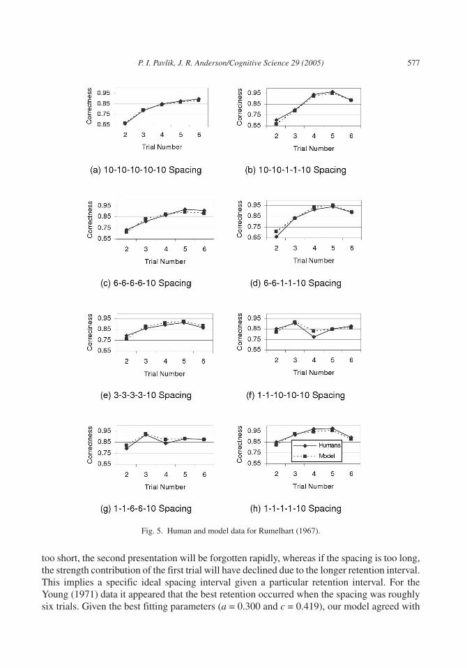
Fig. 5 presents the data Rumelhart (1967) collected and our model of the data. The partici-pants’ results are similar to our experiment. For example, in the 10–10–10–10–10 conditionparticipants learned relatively slowly compared with the 1–1 – 1–1 – 10 condition. However, asour model predicts, after four trials 1–1 – 1–1, the forgetting until the final test after 10 trialswas pronounced compared with the forgetting for the final test after 10 trials with10–10–10–10 spacing. This is evidence that wider spacing resulted in more stable learning asour model implies. First trials are not listed in Fig. 5 because these responses were at chancelevels because participants had no prior practice.

To model these data we assumed each trial was 10 sec long based on Rumelhart’s (1967)methods assuming 5 sec per response. Because guessing had a one-third chance of success,this was included in the model. We estimated the decay parameters (a = 0.149 and c = 0.495) tominimize the χ2 (χ2 = 41.5, df = 38). These decay parameters indicated a relatively high forget-ting rate. This was reasonable considering the stimuli were arguably unmemorable conso-nant–vowel–consonant nonwords, and the responses were easily confusable.

This fit captured the important effects in Fig. 5 (adjusted RMSD = 0.021, r2 = .927). Becauseour model had been developed with different stimuli over durations of days, we considered thegood fit to this data with only two free parameters estimated as evidence in support of ourmodel. These data have also been modeled by Raaijmakers (2003; See Table 3). The fit wasgood (χ2 = 38, df = 34), but note that six parameters were varied. Given the degrees of freedomdifference in the models, this fit was roughly equivalent to the ACT–R fit.

5.3. Young (1971)

In all of our examples so far, wider spacing resulted in better performance later. Young(1971) was one of the first to provide a demonstration that spacing does not always affect per-formance monotonically. In a continuous paired-associate memory experiment, he paired con-sonant trigrams with single digits. Each pair was presented twice for study, with a spacing in-terval of 0 to 17 trials (study trials were 1 sec in duration with a 3-sec intertrial interval). Theretention interval was held constant at 10 trials (40 sec) from the second practice.

The data can be seen in Fig. 6 with a comparison to a fit by the model. This fit captured thenonmonotonic nature of the spacing effect. This result makes sense, because if the spacing is


too short, the second presentation will be forgotten rapidly, whereas if the spacing is too long,the strength contribution of the first trial will have declined due to the longer retention interval.This implies a specific ideal spacing interval given a particular retention interval. For theYoung (1971) data it appeared that the best retention occurred when the spacing was roughlysix trials. Given the best fitting parameters (a = 0.300 and c = 0.419), our model agreed with


Fig. 5. Human and model data for Rumelhart (1967).

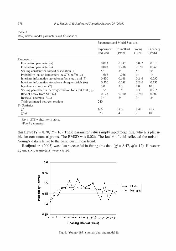
this figure (χ2 = 8.70, df = 16). These parameter values imply rapid forgetting, which is plausi-ble for consonant trigrams. The RMSD was 0.026. The low r2 of .461 reflected the noise inYoung’s data relative to the basic curvilinear trend.

Raaijmakers (2003) was also successful in fitting this data (χ2 = 8.47, df = 12). However,again, six parameters were varied.


Table 3Raaijmakers model parameters and fit statistics

Parameters and Model Statistics

ExperimentReduced

Rumelhart(1967)

Young(1971)

Glenberg(1976)

ParametersFluctuation parameter (a) 0.013 0.087 0.082 0.013Fluctuation parameter (s) 0.047 0.288 0.150 0.260Scaling constant for context association (a) 5a 5a 5a 5a

Probability that an item enters the STS buffer (w) .666 .766 1a 1a

Interitem information stored on a first study trial (b) 0.430 0.688 0.246 0.732Interitem information stored on subsequent trials (b2) 0.570 0.688 0.246 0.732Interference constant (Z) 3.0 3.0 2.0 10.0Scaling parameter in recovery equation for a test trial (θ2) .5a .5a 0.3 0.215Rate of decay from STS (λ) 0.128 0.310 0.746 0.800Retrieval attempts (Lmax) 3a 3a 3a 3a

Trials estimated between sessions 240Fit Statistics

χ2 166 38.0 8.47 41.9χ2 df 23 34 12 18

Note. STS = short-term store.aFixed parameters

Fig. 6. Young (1971) human data and model fit.

5.4. Glenberg (1976; Experiment 1)

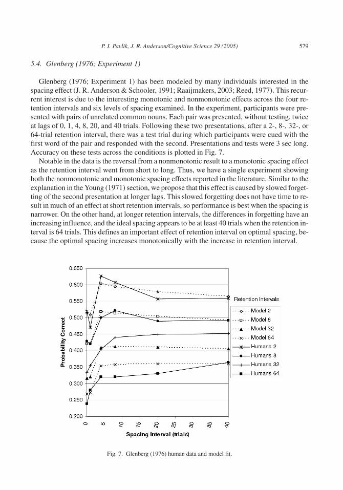
Glenberg (1976; Experiment 1) has been modeled by many individuals interested in thespacing effect (J. R. Anderson & Schooler, 1991; Raaijmakers, 2003; Reed, 1977). This recur-rent interest is due to the interesting monotonic and nonmonotonic effects across the four re-tention intervals and six levels of spacing examined. In the experiment, participants were pre-sented with pairs of unrelated common nouns. Each pair was presented, without testing, twiceat lags of 0, 1, 4, 8, 20, and 40 trials. Following these two presentations, after a 2-, 8-, 32-, or64-trial retention interval, there was a test trial during which participants were cued with thefirst word of the pair and responded with the second. Presentations and tests were 3 sec long.Accuracy on these tests across the conditions is plotted in Fig. 7.

Notable in the data is the reversal from a nonmonotonic result to a monotonic spacing effectas the retention interval went from short to long. Thus, we have a single experiment showingboth the nonmonotonic and monotonic spacing effects reported in the literature. Similar to theexplanation in the Young (1971) section, we propose that this effect is caused by slowed forget-ting of the second presentation at longer lags. This slowed forgetting does not have time to re-sult in much of an effect at short retention intervals, so performance is best when the spacing isnarrower. On the other hand, at longer retention intervals, the differences in forgetting have anincreasing influence, and the ideal spacing appears to be at least 40 trials when the retention in-terval is 64 trials. This defines an important effect of retention interval on optimal spacing, be-cause the optimal spacing increases monotonically with the increase in retention interval.


Fig. 7. Glenberg (1976) human data and model fit.

Incapturing thisexperimentwithourmodel,weneeded todealwith two issues in thedesignofGlenberg’s (1976) Experiment 1. Both of these issues involved the speed of presentation in theexperiment. First, in our experiment, which also used verbal stimuli, the presentation–test inter-val (including intertrial time) was approximately 5 to 10 sec, whereas for this experiment it was 3sec long. Because of these shorter presentations, we scaled the contribution of each presentationby the b parameter, in a fashion identical to the Bahrick (1979) model. Second, we found that thelow performance at lags of 0 and 1 trials (see Fig. 7) was not fitted well by our model. We thoughtthis problem might have been caused by poor encoding of second presentations due to first pre-sentations still being in working memory at these lags of only 0 or 3 sec. According to ACT–R,this item leaves working memory (the goal buffer) automatically on the beginning of each newtrial at which point it is counted as an encoding. Further, our model normally assumes that eachencoding counts equally at its inception, and only decay causes differences in the long-run ef-fects of presentations. Normally these assumptions cause no problems, given a reasonable lag.However, at the very short lags in this experiment, given the relatively easy Glenberg (1976) ma-terial (unlike Young’s experiment, which had short spacings but much more abstract material),we needed to model the possibility that items did not drop from working memory as fast as we as-sumed and thus blocked the full effect of the repetition encoding.

To model this possibility of poorer encoding at these very short lags, we used a reduced br

parameter to scale the contribution of these second presentations. This solution was similar tothe STS mechanism in Raaijmakers’s (2003) model and was necessary to get a quantitativegood fit. Although this mechanism for extremely short lags was ad hoc, we could haveparameterized it as an STS mechanism in a way similar to Raaijmakers. We choose not to dothis because we have no other firm evidence for this mechanism except at these very short lagsin Glenberg’s experiment. Indeed, as Raaijmakers notes, Van Winsum-Westra (1990) was un-able to replicate these dips in performance at very short spacing.

Given these changes, the model fit the data well (χ2 = 31.9, df = 20). The RMSD was 0.026and the r2 was .944. In comparison, the Raaijmakers (2003) model resulted in about the samefit (χ2 = 41.9, df = 18); however, it should be noted that when Raaijmakers made an assumptionsimilar to ours (that 0 lag repetition results in no increase in memory strength) to deal with theshort spacing dips, his χ2 value went down to 28.77. Table 1 shows the parameter values, andFig. 7 shows the fit of our model to the data. Although the result shows some deviation, it is no-table that our model captures the effect of retention interval on optimal spacing (and it capturedthis effect before we made any of the changes in the preceding paragraph). Raaijmakers’(2003) model did not capture this interaction. Further, his model used two more parameters.

6. General discussion

Our experiment produced data to test alternative models of practice, forgetting, and thespacing effect. These data confirmed the standard spacing effect in various conditions andshowed that wide spacing of practice provides increasing benefit as practice accumulates. Fur-ther, the strong crossover interactions produced provided evidence that people forget less whenpresentations are widely spaced. The findings of this experiment were used to extend ACT–R’sactivation equation by introducing a variable decay-rate function. According to this mecha-nism, the forgetting rate for each presentation of a memory chunk is a function of the activation


of the chunk at the time of the presentation. Using this model, we fitted data from our experi-ment and four experiments from the literature. These fits demonstrated the viability of ourmechanism and showed that with the other ACT–R equations it provides an accurate model ina wide variety of conditions. To show that our model was at least as good as an alternativemodel, we compared our fits for some experiments with fits of the Raaijmakers (2003) model.We were able to produce comparable fits to existing experiments, a better fit to our own experi-ment, and overall our models had less variation in fewer parameters.

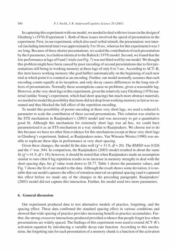
The graphs that we showed for our own experiment aggregated over the two retention inter-vals, so it may not be immediately clear that the crossover spacing by retention-interval inter-action occurred rapidly after final test trials. Fig. 8 shows the predictions of our model for re-call at various retention intervals for each spacing condition. These model values and theobserved recall at 1- and 7-day retention intervals show the performance we predicted or ob-served on initial test trials for sessions begun at these retention intervals. This figure makes itclear that the crossover interaction has occurred before the 1-day retention interval session be-gins. The speed with which the crossovers occur makes sense, given our proposal that differentpower-law decay values control each retention function. Because the loss rate of memoryslows down in power-law forgetting, the greatest changes in strength between the conditionsshould occur soon after learning.

Given the properties of our model, it is interesting to speculate about what physiologicalmechanisms might be producing these effects. There are some suggestions that neural plastic-ity has the features of our model. For instance, in regard to our new decay mechanism, there iswork that shows that LTP of neurons declines less rapidly when there is spaced induction ofLTP rather than massed induction (Scharf et al., 2002). This result is similar to Wu, Deisseroth,& Tsien (2001) in which spaced stimulation resulted in dendritic changes consistent with


Fig. 8. Predictions of the model (including the relevant data points) for first trials of second sessions begun after therespective retention intervals. Values exclude the eight-test trial condition and aggregate repetition conditions. 1 SEconfidence intervals computed from participant means.

long-term memory formation, whereas massed stimulation did not have such an effect. Prop-erties of LTP may also correspond to other aspects of our model. For instance, Beggs (2000)presented a statistical model of LTP, proposing that the magnitude of the LTP induced by stim-ulation is negatively related to this postsynaptic activation. This occurs because increases inLTP in his model are controlled by the discrepancy between presynaptic input and pos-tsynaptic activation. This discrepancy is reduced with LTP induction, and thus subsequentchanges in LTP are less. Our model captures this principle by taking the logarithm of the com-bined trace, thus new encodings add less to activation if it is already high.

In fact, Landauer (1969) has proposed a neural consolidation theory of the spacing effect.In this theory, presenting an item (P1) results in a “hyperexcitable” state in the nervous sys-tem following the presentation. This decaying hyperexcitability, according to Landauer,gradually promotes changes in the nervous system responsible for permanent representationof the association. During this period of consolidation, a new presentation (P2) of the samepairing will interrupt the consolidation of P1 due to systemic limits on hyperexcitability. Be-cause of this, the less spacing of presentations, the less memory is strengthened. AsHintzman (1974) pointed out, consolidation theory suffers from a lack of agreement withdata that show it is P2 learning that suffers rather than P1 when spacing is narrow. Our ver-sion, by placing the effect at P2 rather than P1, no longer suffers from the problems thatHintzman discussed.

Discussing a possible neural basis of the spacing effect suggests an involuntary process.Hintzman (1974) took the broad generality of the spacing effect as evidence that it is not undervoluntary control. He proposed that habituation with a stimulus caused it to have less of an ef-fect on increasing long-term memory. Because habituation decreases with time, spaced trialsincur a benefit. Although he suggested that massed practice would result in “a decrease in thestrength of any new trace that is formed” (Hintzman, 1974, p. 90), he also recognized that theeffect occurred for the storage of long-term memories. Thus, although he did not give a formalmodel, his idea that habituation controls the long-term strength benefit of a spaced practice issimilar to our proposal that activation controls the forgetting rate.

The model we have described also agrees with cognitive theories of the spacing effect,which say that the benefit of additional practice is mediated by the difficulty or accessibility ofthat additional practice. This sort of accessibility theory has been advocated by various re-searchers (Cuddy & Jacoby, 1982; Schmidt & Bjork, 1992; Whitten & Bjork, 1977). These re-searchers have noted that manipulations that cause slower acquisition often result in betterlong-term retention. This paradox occurs in many experimental situations. For instance,Schneider, Healy, and Bourne (2002) conjectured that the greater difficulty participants hadlearning foreign language responses (as opposed to English responses) in a paired-associateexperiment may have produced better long-term recollection. This result makes sense if wesuppose greater difficulty indicates lower activation. Thus, a manipulation that increases diffi-culty might be modeled as a penalty to activation. This lower effective activation would resultin less forgetting and therefore better long-term retention.

Although this notion that less accessibility at practice results in better long-term recall is nota new idea, we have presented here the first detailed computational model of how this mightoccur. We feel this model serves to clarify the theoretical discussion about the effects of prac-tice by allowing clear quantitative and qualitative comparisons to other theories of practice and


forgetting such as those proposed by advocates of contextual fluctuation mechanisms. Thisformal model of the relation between current memory accessibility and the stability of newencodings, using an integrative retention function, provided good fits to a wide variety of re-sults with estimation of only a minimal number of parameters. Further, the absolute and rela-tive parameter stability of the model shows that the model’s behavior was consistent with dif-ferent data sets. This parameter stability enhances the explanatory utility of the model foraddressing the broad theoretical issues underlying practice and forgetting.

Notes

1. Exact trial order for the experiment and working models for all experiments can befound at http://act-r.psy.cmu.edu/models/.

2. This is different from the typical paired-associate procedure that usually also includes astudy after successful recall. In a recent study (Pavlik & Anderson, 2004), we comparedour procedure with the typical procedure and found long-term differences of less than2% in recall after multiple practices. Because a study after a successful recall is at a veryshort spacing, this result is consistent with our model.

3. In ACT–R individual strengthenings are considered to be discrete when the encodinginterval is reasonably long. This corresponds to data, such as Melton (1970), whichshow that as the presentation interval increases, the length of the presentation intervalhas less effect on final performance. Encoding appears to have quickly diminishingmarginal returns. We introduce a b parameter that scales the contribution of each t i

di� inthe fits for Glenberg (1976) and Bahrick (1979) later in this article to deal with specificmethods used in these experiments. This b value is equal to 1 in a standard ACT–Rmodel.

4. The logarithm of the sum is taken to yield observed retention functions and provides acorrespondence with log odds of items occurring in the environment as shown by J. R.Anderson and Schooler, 1991. For an extensive review of the mathematical character-ization of this system, the reader is referred to Chapter 3 of The Atomic Components ofThought (J. R. Anderson & Lebiere, 1998, Appendix A).

5. It should be noted that the psychological time factor in this article takes a slightly differ-ent form as compared to J. R. Anderson et al. (1999). In this conception, we take the hfactor to be a direct scaling parameter of the time between experimental sessions.

6. Note that because retrieval time in ACT–R is proportional to e–m, Equation 4 makes de-cay an inverse function of retrieval time.

7. The idea that neural consolidation processes depend on spacing is supported by severalsources such as Scharf et al. (2002) and Wu et al. (2001).

Acknowledgments

This research was funded by National Science Foundation Grant BCS 997–5-220. Portionsof this work were presented at Fifth International Conference of Cognitive Modeling,Bamberg, Germany.


References

Anderson, J. R., Fincham, J. M., & Douglass, S. (1999). Practice and retention: A unifying analysis. Journal of Ex-perimental Psychology: Learning, Memory, and Cognition, 25, 1120–1136.

Anderson, J. R., & Lebiere, C. (1998). The atomic components of thought. Mahwah, NJ: Lawrence Erlbaum Associ-ates, Inc.

Anderson, J. R., & Schooler, L. J. (1991). Reflections of the environment in memory. Psychological Science, 2,396–408.

Anderson, R. B., & Tweney, R. D. (1997). Artifactual power curves in forgetting. Memory and Cognition, 25,724–730.

Atkinson, R. C., & Shiffrin, R. M. (1968). Human memory: A proposed system and its control processes. In K. W.Spence & J. T. Spence (Eds.), The psychology of learning and motivation: II (pp. 89–195). Oxford, England: Ac-ademic.

Bahrick, H. P. (1979). Maintenance of knowledge: Questions about memory we forgot to ask. Journal of Experi-mental Psychology: General, 108, 296–308.

Bahrick, H. P. (1984). Semantic memory content in permastore: Fifty years of memory for Spanish learned inschool. Journal of Experimental Psychology: General, 113, 1–29.

Bahrick, H. P., & Phelps, E. (1987). Retention of Spanish vocabulary over 8 years. Journal of Experimental Psy-chology: Learning, Memory, and Cognition, 13, 344–349.

Beggs, J. M. (2000). A statistical theory of long-term potentiation and depression. Neural Computation, 13,87–111.

Bogartz, R. S. (1990). Evaluating forgetting curves psychologically. Journal of Experimental Psychology:Learning, Memory, and Cognition, 16, 138–148.

Carrier, M., & Pashler, H. (1992). The influence of retrieval on retention. Memory and Cognition, 20, 633–642.Coltheart, M. (1981). The MRC psycholinguistic database. Quarterly Journal of Experimental Psychology: Human

Experimental Psychology, 33, 497–505.Cuddy, L. J., & Jacoby, L. L. (1982). When forgetting helps memory: An analysis of repetition effects. Journal of

Verbal Learning and Verbal Behavior, 21, 451–467.Delaney, P. F., Reder, L. M., Staszewski, J. J., & Ritter, F. E. (1998). The strategy-specific nature of improvement:

The power law applies by strategy within task. Psychological Science, 9, 1–7.Ebbinghaus, H. (1885). Über das Gedachtnis: Untersuchungen zur Experimentellen Psychologie. Leipzig, Ger-

many: Duncker & Humblot.Estes, W. K. (1955). Statistical theory of distributional phenomena in learning. Psychological Review, 62, 369–377.Geinisman, Y. (2000). Structural synaptic modifications associated with hippocampal LTP and behavioral learning.

Cerebral Cortex, 10, 952–962.Glenberg, A. M. (1976). Monotonic and nonmonotonic lag effects in paired-associate and recognition memory par-

adigms. Journal of Verbal Learning and Verbal Behavior, 15, 1–16.Glenberg, A. M. (1979). Component-levels theory of the effects of spacing of repetitions on recall and recognition.

Memory and Cognition, 7, 95–112.Glenberg, A. M., & Smith, S. M. (1981). Spacing repetitions and solving problems are not the same. Journal of Ver-

bal Learning and Verbal Behavior, 20, 110–119.Heathcote, A., Brown, S., & Mewhort, D. J. K. (2000). The power law repealed: The case for an exponential law of

practice. Psychonomic Bulletin and Review, 7, 185–207.Hintzman, D. L. (1974). Theoretical implications of the spacing effect. In R. L. Solso (Ed.), Theories in cognitive

psychology: The Loyola Symposium (pp. 77–99). Oxford, England: Lawrence Erlbaum Associates, Inc.Landauer, T. K. (1969). Reinforcement as consolidation. Psychological Review, 76, 82–96.Logan, G. D. (1992). Shapes of reaction-time distributions and shapes of learning curves: A test of the instance the-

ory of automaticity. Journal of Experimental Psychology: Learning, Memory, and Cognition, 18, 883–914.Melton, A. W. (1970). The situation with respect to the spacing of repetitions and memory. Journal of Verbal

Learning and Verbal Behavior, 9, 596–606.


Newell, A., & Rosenbloom, P. S. (1981). Mechanisms of skill acquisition and the law of practice. In J. R. Anderson(Ed.), Cognitive skills and their acquisition (pp. 1–55). Hillsdale, NJ: Lawrence Erlbaum Associates, Inc.

Nikonenko, I., Jourdain, P., & Muller, D. (2003). Presynaptic remodeling contributes to activity-dependentsynaptogenesis. Journal of Neuroscience, 23, 8498–8505.

Pavlik, P. I., Jr., & Anderson, J. R. (2004, August). The memory consequences of study after successful recall. Paperpresented at the twenty-sixth annual conference of the Cognitive Science Society, Chicago.

Pitt, M. A., Myung, I. J., & Zhang, S. (2002). Toward a method of selecting among computational models of cogni-tion. Psychological Review, 109, 472–491.

Raaijmakers, J. G., & Shiffrin, R. M. (1981). Search of associative memory. Psychological Review, 88, 93–134.Raaijmakers, J. G. W. (2003). Spacing and repetition effects in human memory: Application of the SAM model.

Cognitive Science, 27, 431–452.Reed, A. V. (1977). Quantitative prediction of spacing effects in learning. Journal of Verbal Learning and Verbal

Behavior, 16, 693–698.Rickard, T. C. (1997). Bending the power law: A CMPL theory of strategy shifts and the automatization of cognitive

skills. Journal of Experimental Psychology: General, 126, 288–311.Ross, B. H., & Landauer, T. K. (1978). Memory for at least one of two items: Test and failure of several theories of

spacing effects. Journal of Verbal Learning and Verbal Behavior, 17, 669–680.Rubin, D. C., & Wenzel, A. E. (1996). One hundred years of forgetting: A quantitative description of retention. Psy-

chological Review, 103, 734–760.Rumelhart, D. E. (1967). The effects of interpresentation intervals on performance in a continuous paired-associate

task (Tech. Rep. No. 16). Stanford, CA: Stanford University, Institute for Mathematical Studies in Social Sci-ences.

Scharf, M. T., Woo, N. H., Lattal, K. M., Young, J. Z., Nguyen, P. V., & Abel, T. (2002). Protein synthesis is requiredfor the enhancement of long-term potentiation and long-term memory by spaced training. Journal ofNeurophysiology, 87, 2770–2777.

Schmidt, R. A., & Bjork, R. A. (1992). New conceptualizations of practice: Common principles in three paradigmssuggest new concepts for training. Psychological Science, 3, 207–217.

Schneider, V. I., Healy, A. F., & Bourne, L. E. J. (2002). What is learned under difficult conditions is hard to forget:Contextual interference effects in foreign vocabulary acquisition, retention, and transfer. Journal of Memory andLanguage, 46, 419–440.

Toni, N., Buchs, P. A., Nikonenko, I., Povilaitite, P., Parisi, L., & Muller, D. (2001) Remodeling of synaptic mem-branes following induction of long-term potentiation. Journal of Neuroscience, 21, 6245–6251.

Underwood, B. J. (1969). Some correlates of item repetition in free-recall learning. Journal of Verbal Learning andVerbal Behavior, 8, 83–94.

VanWinsum-Westra, M. (1990). Spacing and repetition effects in human memory. Unpublished doctoral disserta-tion, University of Nijmegen, The Netherlands.

Whitten, W. B., & Bjork, R. A. (1977). Learning from tests: Effects of spacing. Journal of Verbal Learning and Ver-bal Behavior, 16, 465–478.

Wickelgren, W. A. (1973). The long and the short of memory. Psychological Bulletin, 80, 425–438.Wickelgren, W. A. (1974). Single-trace fragility theory of memory dynamics. Memory and Cognition, 2, 775–780.Wickens, T. D. (1999). Measuring the time course of retention. In C. Izawa (Ed.), On human memory: Evolution,

progress, and reflections on the 30th anniversary of the Atkinson-Shiffrin model (pp. 245–266). Mahwah, NJ:Lawrence Erlbaum Associates, Inc.

Wixted, J. T., & Ebbesen, E. B. (1997). Genuine power curves in forgetting: A quantitative analysis of individualsubject forgetting functions. Memory and Cognition, 25, 731–739.

Woodworth, R. S. (1938). Experimental psychology. Oxford, England: Holt.Wu, G., Deisseroth, K., & Tsien, R. W. (2001). Spaced stimuli stabilize MAPK pathway activation and its effects on

dendritic morphology. Nature Neuroscience, 4, 151–158.Young, J. L. (1971). Reinforcement-test intervals in paired-associate learning. Journal of Mathematical Psychol-

ogy, 8, 58–81.


Appendix

Because the math underlying the computation is recursive and a bit complex, the followingis an example of the activation and decay computations involved for the session one 14-spacingcondition with two tests. This example also includes two tests on the second session. This is asequence of five presentations, the first being the introductory study and the remaining four be-ing test trials. The long-term retention interval (1 day) is interposed between the third andfourth tests.

The actual average times of this sequence of practice are approximately: 0; 126; 252;83,855; and 84,888. This indicates that the first study occurs at time 0. The last two times in-clude the 22.5 hr between the end of the first session and the beginning of the second, which is81,000 sec. To account for the reduced forgetting over this interval we need to multiply the81,000 sec by the h factor (.025), resulting in a scaled value of 2,025. This means that the timesafter the long interval need to be reduced by 78,975 (the difference between the actual and psy-chological times) to convert them to a measure of psychological time. This results in the se-quence 0; 126; 252; 4,844; 5,877.

Now the activation at each test time can be computed. At Time 126 the first test occurs; ac-cording to Equations 4 and 5, m1 = ln(126–0.177) = –0.86. Recall that the decay from the firststudy (d1) is simply a.

To compute the activation of the second test, we need to use the activation at the time of thefirst test to compute the decay for that presentation. Using Equation 4, d2 = ce m1 + a, whichequals 0.27. Since the age of the initial study is now 252, and the age of the first test is 126,from Equation 5 we get m2 = ln(252–0.177 + 126–0.27) = –0.43.

To compute the activation of the third test we now need to compute d3, which is ce m2 + a =0.32. The age of the first presentation is now 4,844, the age of the second presentation is 4,717,and the age of the third presentation is 4,591. Therefore activation m3 is ln(4,844–0.177 +4,717–0.27 + 4,591–0.32) = –0.93.

For the final test in this example sequence we need to compute the decay for the third test(fourth presentation), d4 = ce m3 + a = 0.26. The sequence of ages is 5,877; 5,750; 5,624; and1,033. Activation m4 is ln(5,877–0.177 + 5,750–0.27 + 5,624–0.32 + 1,033–0.26), which equals –0.62.


Documents

Practice and Forgetting Effects on Vocabulary Memory: …act-r.psy.cmu.edu/wordpress/wp-content/uploads/2012/12/409s... · Practice and Forgetting Effects on Vocabulary Memory: An