Embed Size (px)
DESCRIPTION
Practice. Situation 1 Based on a sample of 100 subjects you find the correlation between extraversion is happiness is r=.15. Determine if this value is significantly different than zero. Situation 2 - PowerPoint PPT Presentation
Citation preview

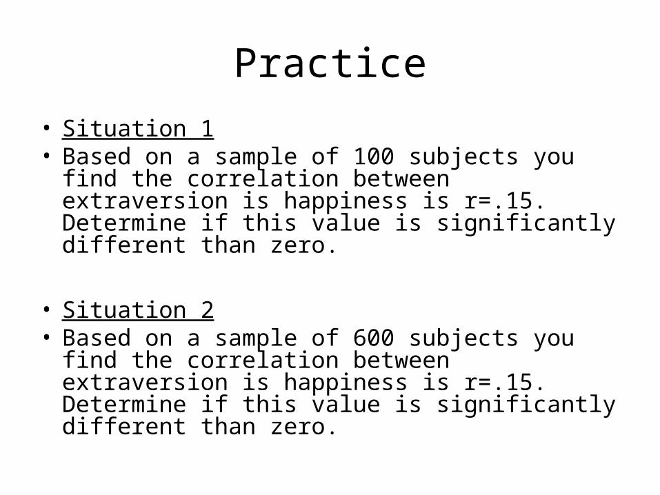
Practice
• Situation 1• Based on a sample of 100 subjects you find the
correlation between extraversion is happiness is r=.15. Determine if this value is significantly different than zero.
• Situation 2• Based on a sample of 600 subjects you find the
correlation between extraversion is happiness is r=.15. Determine if this value is significantly different than zero.
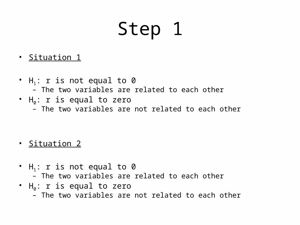
Step 1• Situation 1
• H1: r is not equal to 0– The two variables are related to each other
• H0: r is equal to zero– The two variables are not related to each other
• Situation 2
• H1: r is not equal to 0– The two variables are related to each other
• H0: r is equal to zero– The two variables are not related to each other
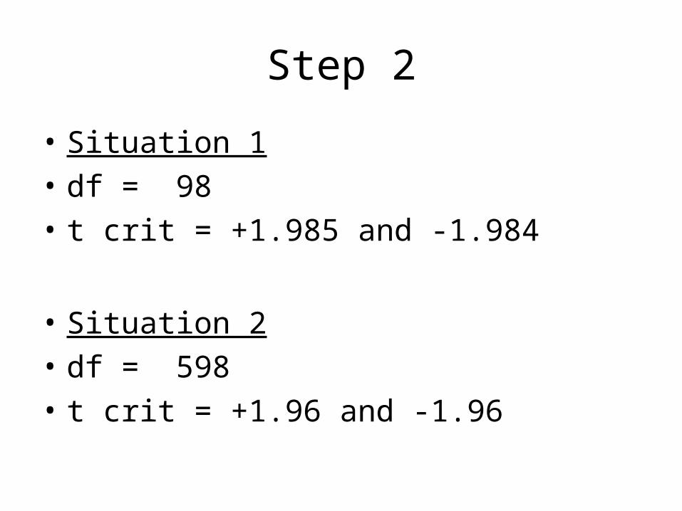
Step 2
• Situation 1
• df = 98
• t crit = +1.985 and -1.984
• Situation 2
• df = 598
• t crit = +1.96 and -1.96
Step 3
• Situation 1
• r = .15
• Situation 2
• r = .15
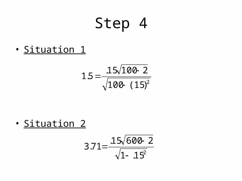
Step 4
• Situation 1
• Situation 2
2)15(.100
210015.5.1
215.1
260015.71.3
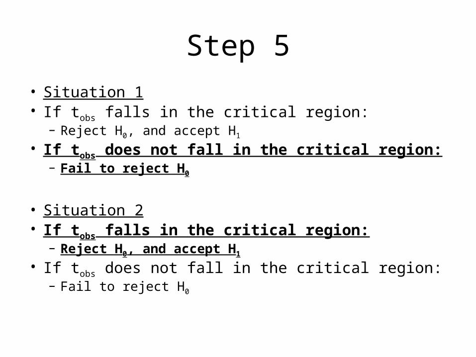
Step 5
• Situation 1• If tobs falls in the critical region:
– Reject H0, and accept H1
• If tobs does not fall in the critical region:– Fail to reject H0
• Situation 2• If tobs falls in the critical region:
– Reject H0, and accept H1
• If tobs does not fall in the critical region:– Fail to reject H0
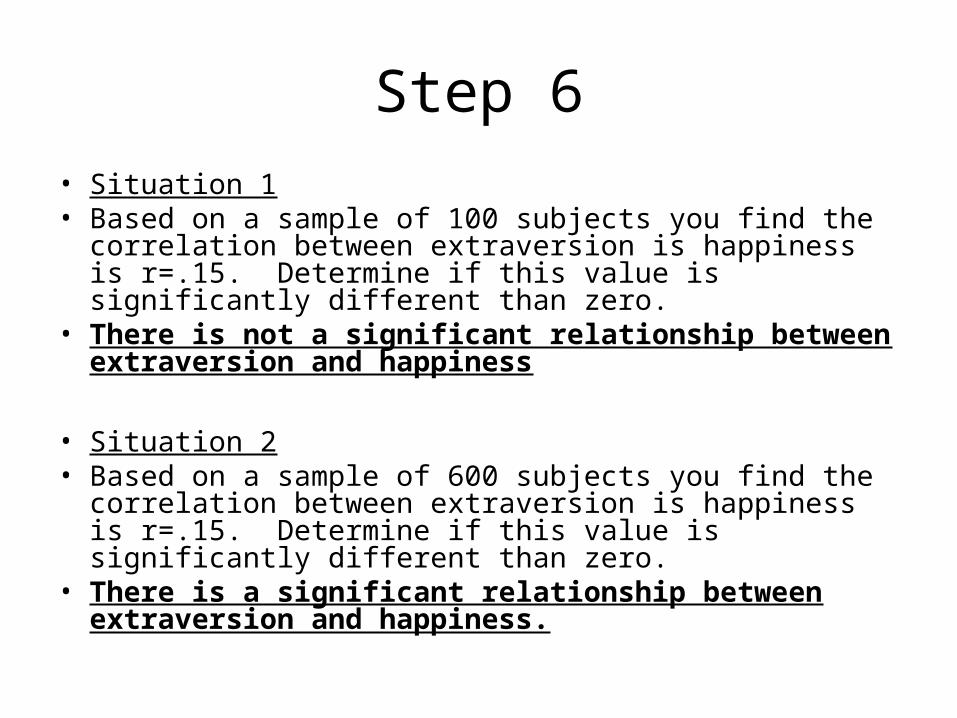
Step 6
• Situation 1• Based on a sample of 100 subjects you find the
correlation between extraversion is happiness is r=.15. Determine if this value is significantly different than zero.
• There is not a significant relationship between extraversion and happiness
• Situation 2• Based on a sample of 600 subjects you find the
correlation between extraversion is happiness is r=.15. Determine if this value is significantly different than zero.
• There is a significant relationship between extraversion and happiness.
Practice
• You collect data from 53 females and find the correlation between candy and depression is -.40. Determine if this value is significantly different than zero.
• You collect data from 53 males and find the correlation between candy and depression is -.50. Determine if this value is significantly different than zero.

Practice
• You collect data from 53 females and find the correlation between candy and depression is -.40.– t obs = 3.12 – t crit = 2.00
• You collect data from 53 males and find the correlation between candy and depression is -.50.– t obs = 4.12– t crit = 2.00
Practice
• You collect data from 53 females and find the correlation between candy and depression is -.40.
• You collect data from 53 males and find the correlation between candy and depression is -.50.
• Is the effect of candy significantly different for males and females?
Hypothesis
• H1: the two correlations are different
• H0: the two correlations are not different
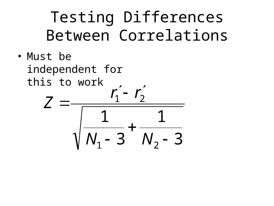
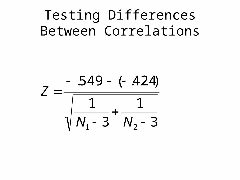
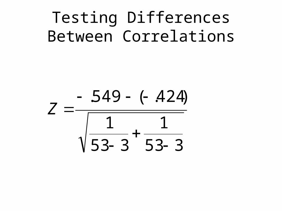
Testing Differences Between Correlations
• Must be independent for this to work
31
31
21
21
NN
rrZ
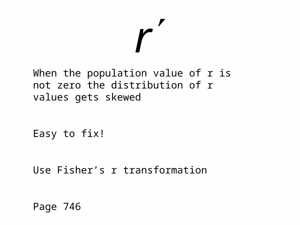
rWhen the population value of r is not zero the distribution of r values gets skewed
Easy to fix!
Use Fisher’s r transformation
Page 746

Testing Differences Between Correlations
• Must be independent for this to work
31
31
21
21
NN
rrZ
Testing Differences Between Correlations
31
31
)424.(549.
21
NN
Z
Testing Differences Between Correlations
3531
3531
)424.(549.
Z
Testing Differences Between Correlations
3531
3531
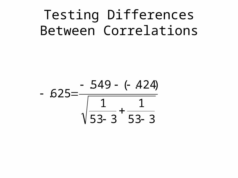
)424.(549.625.
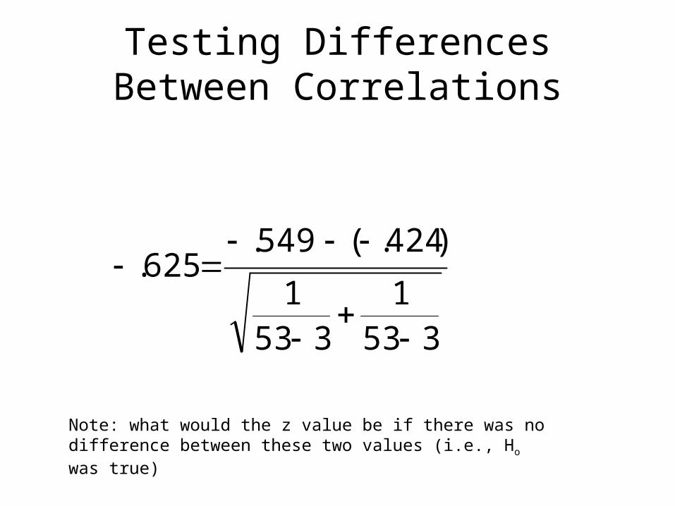
Testing Differences Between Correlations
3531
3531
)424.(549.625.
Note: what would the z value be if there was no difference between these two values (i.e., Ho was true)
Testing Differences
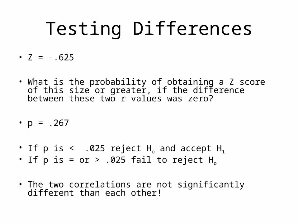
• Z = -.625
• What is the probability of obtaining a Z score of this size or greater, if the difference between these two r values was zero?
• p = .267
• If p is < .025 reject Ho and accept H1
• If p is = or > .025 fail to reject Ho
• The two correlations are not significantly different than each other!


Remember this:Statistics Needed
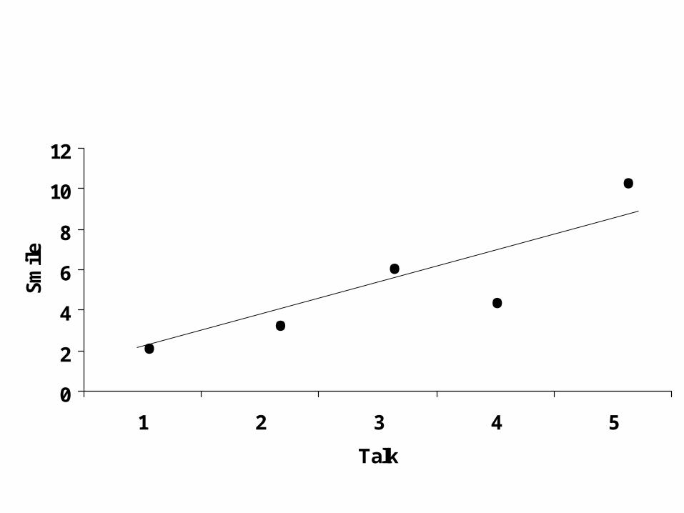
• Need to find the best place to draw the regression line on a scatter plot
• Need to quantify the cluster of scores around this regression line (i.e., the correlation coefficient)
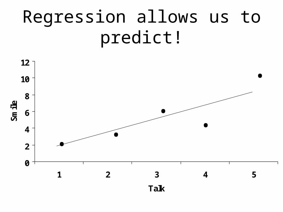
Regression allows us to predict!
0
2
4
6
8
10
12
1 2 3 4 5
Talk
Smile
.
.. ..

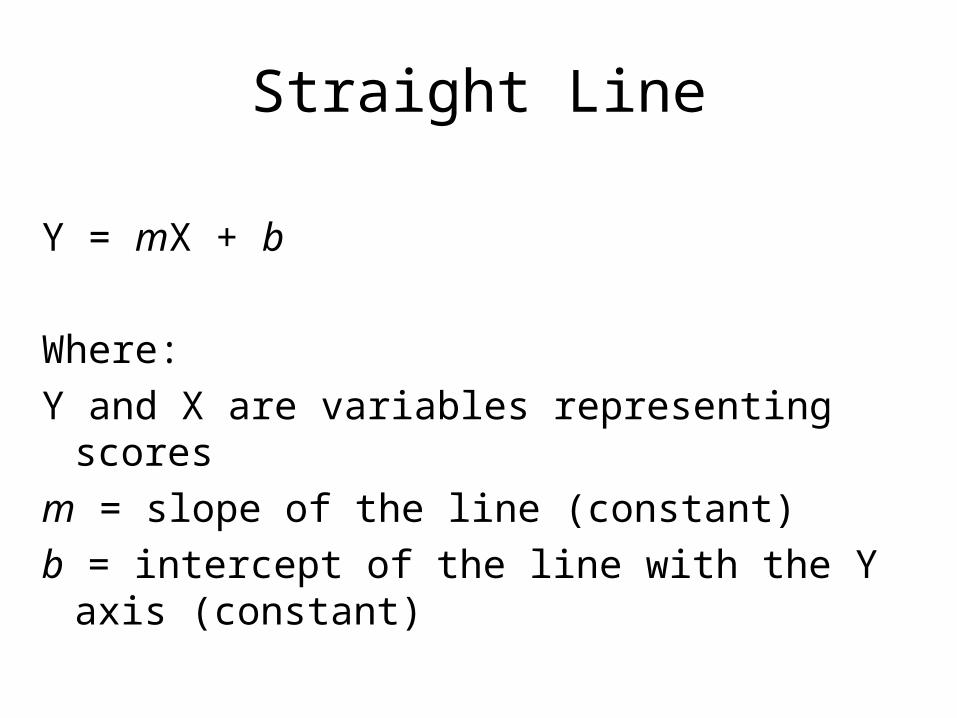
Straight Line
Y = mX + b
Where:
Y and X are variables representing scores
m = slope of the line (constant)
b = intercept of the line with the Y axis (constant)

Excel Example
That’s nice but. . . .
• How do you figure out the best values to use for m and b ?
• First lets move into the language of regression
Straight Line
Y = mX + b
Where:
Y and X are variables representing scores
m = slope of the line (constant)
b = intercept of the line with the Y axis (constant)

Regression Equation
Y = a + bX
Where:
Y = value predicted from a particular X value
a = point at which the regression line intersects the Y axis
b = slope of the regression line
X = X value for which you wish to predict a Y value

Practice
• Y = -7 + 2X
• What is the slope and the Y-intercept?
• Determine the value of Y for each X:
• X = 1, X = 3, X = 5, X = 10
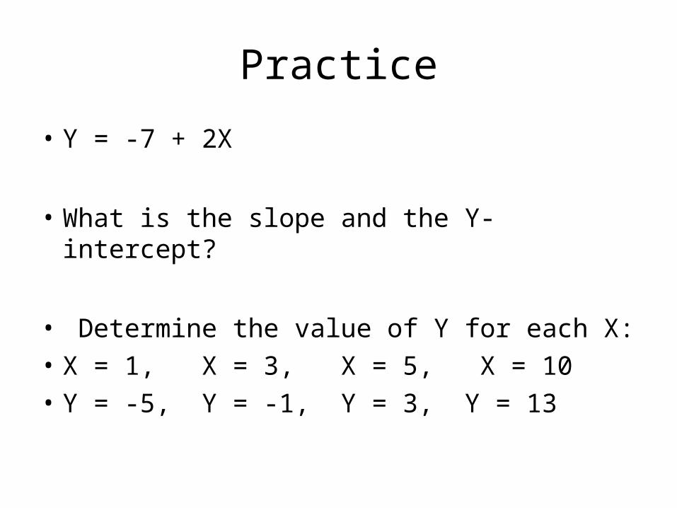
Practice
• Y = -7 + 2X
• What is the slope and the Y-intercept?
• Determine the value of Y for each X:
• X = 1, X = 3, X = 5, X = 10
• Y = -5, Y = -1, Y = 3, Y = 13
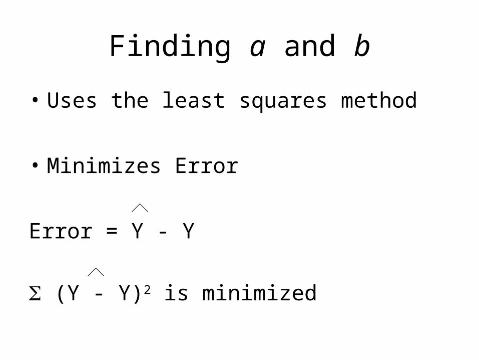
Finding a and b
• Uses the least squares method
• Minimizes Error
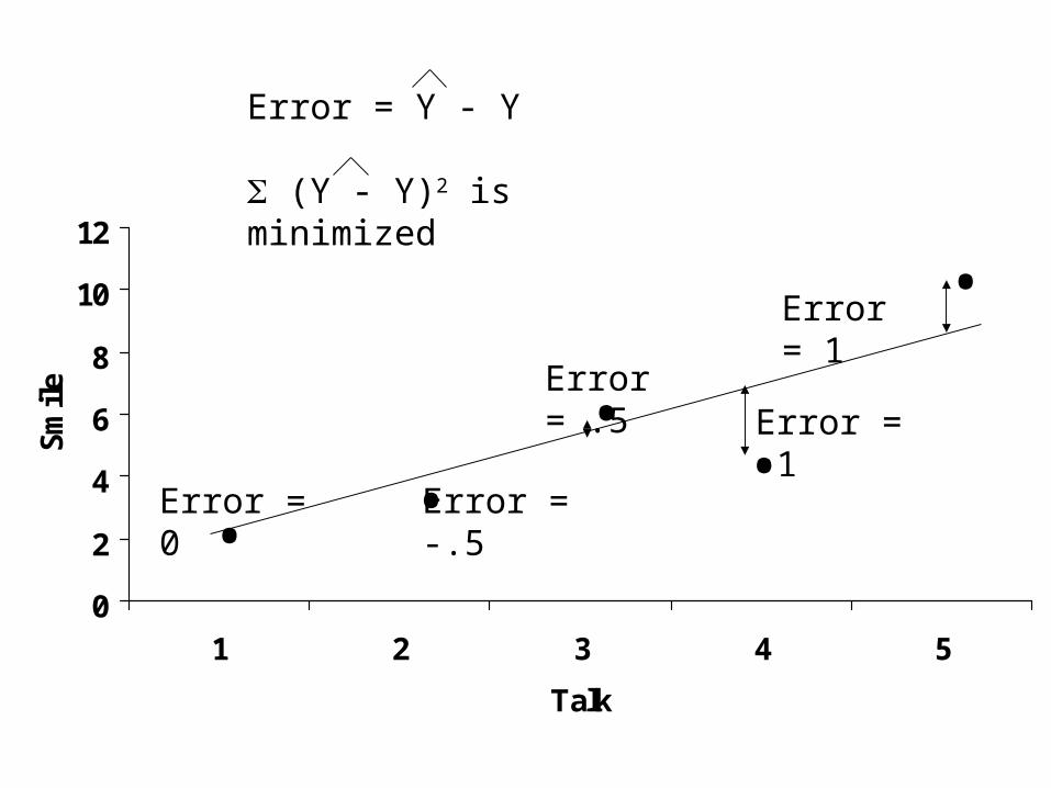
Error = Y - Y
(Y - Y)2 is minimized
0
2
4
6
8
10
12
1 2 3 4 5
Talk
Smile
.
.. ..

0
2
4
6
8
10
12
1 2 3 4 5
Talk
Smile
.
.. ..
Error = 1
Error = -1Error = .5
Error = -.5Error = 0
Error = Y - Y
(Y - Y)2 is minimized

Finding a and b
• Ingredients
• COVxy
• Sx2
• Mean of Y and X
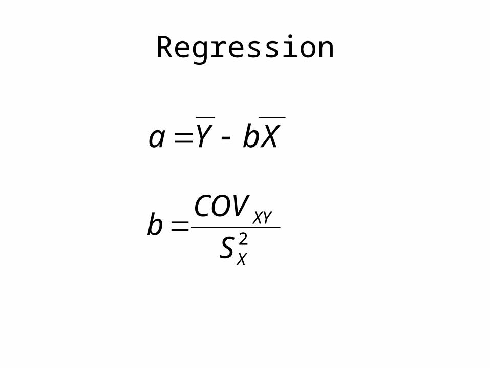
Regression
XbYa
2X
XY
S
COVb
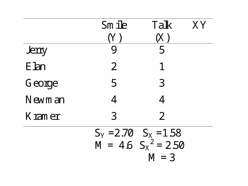
Smile (Y)
Talk (X)
XY
Jerry 9 5
Elan 2 1
George 5 3
Newman 4 4
Kramer 3 2
SY =2.70 M = 4.6
SX =1.58 SX
2 = 2.50 M = 3

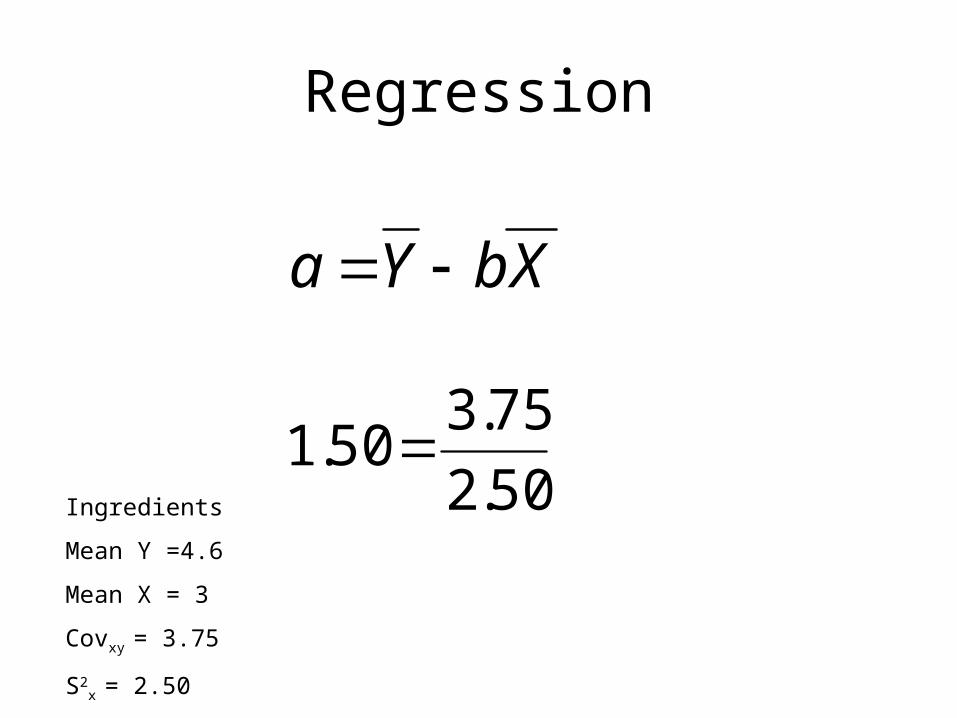
Regression
XbYa
2X
XY
S
COVb
Ingredients
Mean Y =4.6
Mean X = 3
Covxy = 3.75
S2X = 2.50
Regression
XbYa
50.2
75.350.1
Ingredients
Mean Y =4.6
Mean X = 3
Covxy = 3.75
S2x = 2.50
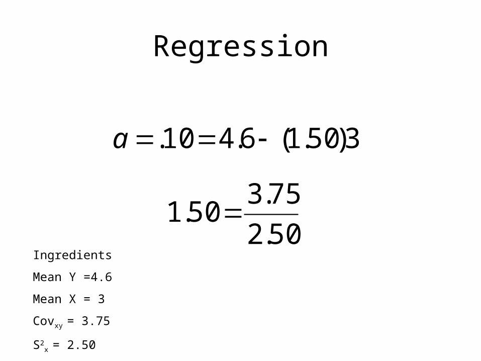
Regression
3)50.1(6.410. a
Ingredients
Mean Y =4.6
Mean X = 3
Covxy = 3.75
S2x = 2.50
50.2
75.350.1
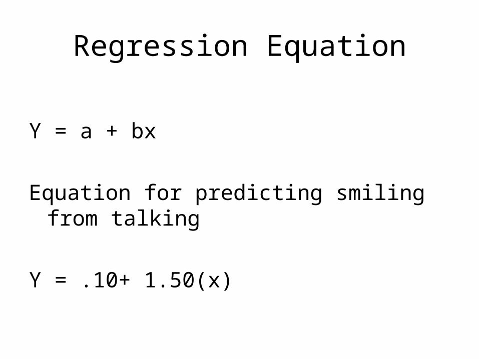
Regression Equation
Y = a + bx
Equation for predicting smiling from talking
Y = .10+ 1.50(x)

1.000E-01 1.567 .064 .953
1.500 .473 .878 3.174 .050
(Constant)
TALK
Model1
B Std. Error
UnstandardizedCoefficients
Beta
Standardized
Coefficients
t Sig.
Coefficientsa
Dependent Variable: SMILEa.
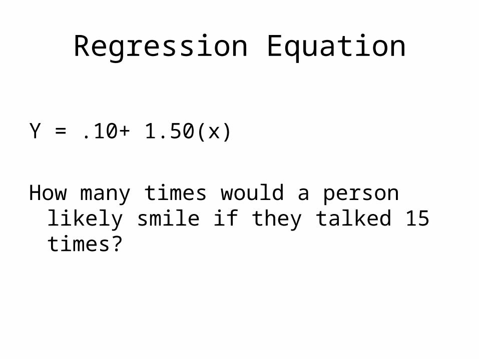
Regression Equation
Y = .10+ 1.50(x)
How many times would a person likely smile if they talked 15 times?
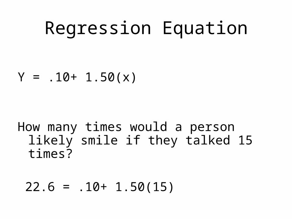
Regression Equation
Y = .10+ 1.50(x)
How many times would a person likely smile if they talked 15 times?
22.6 = .10+ 1.50(15)
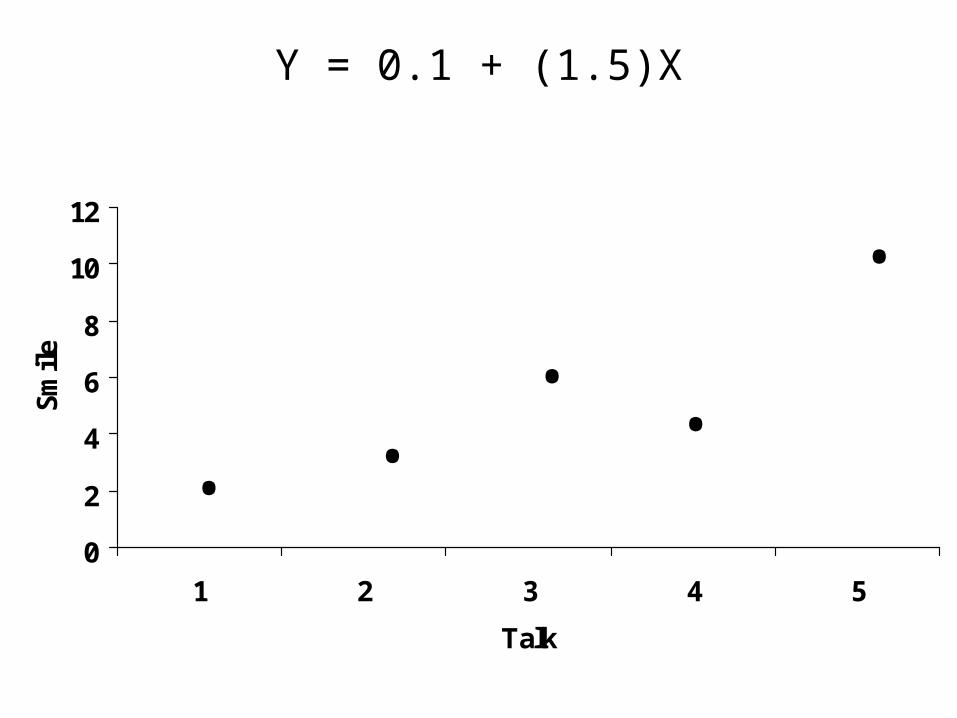
0
2
4
6
8
10
12
1 2 3 4 5
Talk
Smile
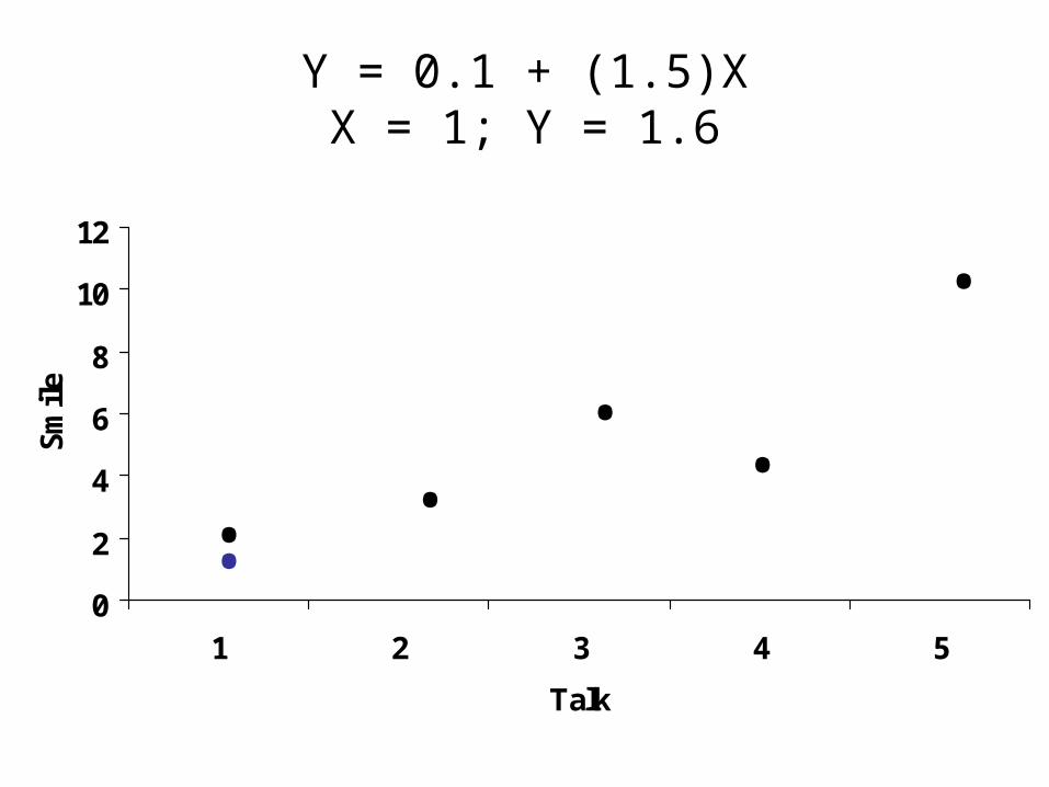
Y = 0.1 + (1.5)X
.
.. ..
0
2
4
6
8
10
12
1 2 3 4 5
Talk
Smile
Y = 0.1 + (1.5)XX = 1; Y = 1.6
.
.
.. ..

0
2
4
6
8
10
12
1 2 3 4 5
Talk
Smile
Y = 0.1 + (1.5)XX = 5; Y = 7.60
.
.
.
.. ..

0
2
4
6
8
10
12
1 2 3 4 5
Talk
Smile
Y = 0.1 + (1.5)X
.
.
.
.. ..

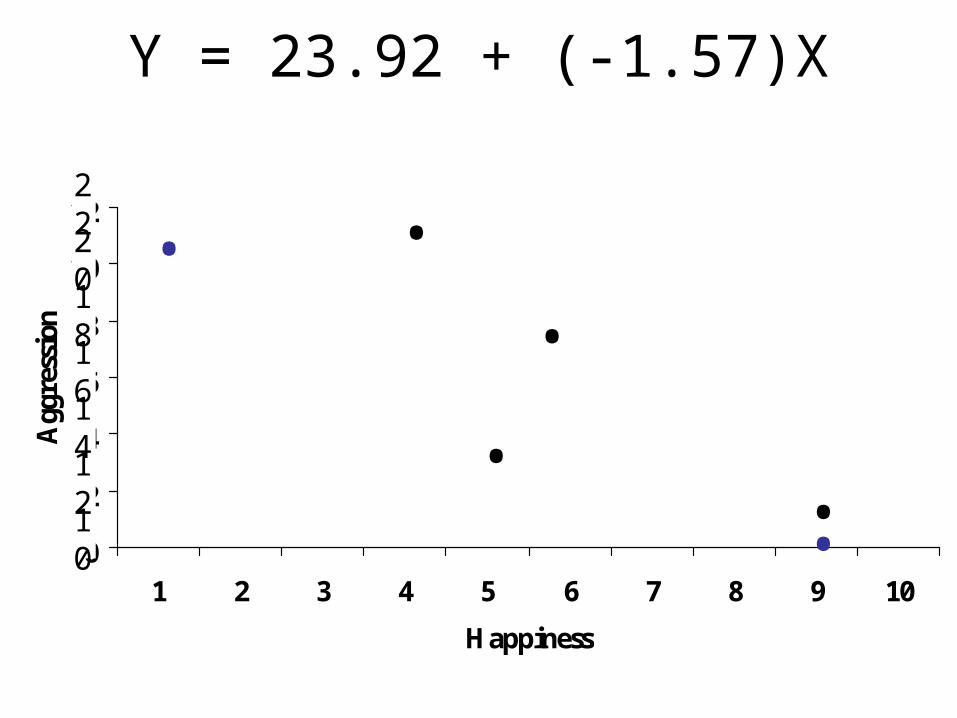
Aggression Y
Happiness X
Mr. Blond 10 9
Mr. Blue 20 4
Mr. Brown 12 5
Mr. Pink 16 6
Mean Y = 14.50; Sy = 4.43Mean X = 6.00; Sx= 2.16
Quantify the relationship with a correlation and draw a regression line that predicts aggression.
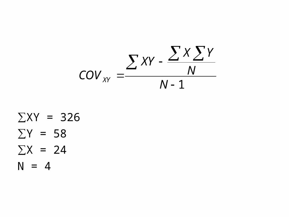
∑XY = 326
∑Y = 58
∑X = 24
N = 4
1
NN
YXXY
COVXY
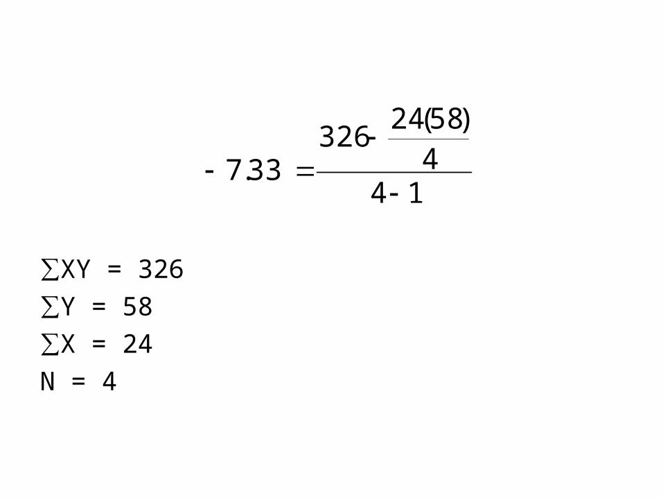
∑XY = 326
∑Y = 58
∑X = 24
N = 4
144
)58(24326
33.7

• COV = -7.33
• Sy = 4.43Sx= 2.16
YX
XY
SS
COVr
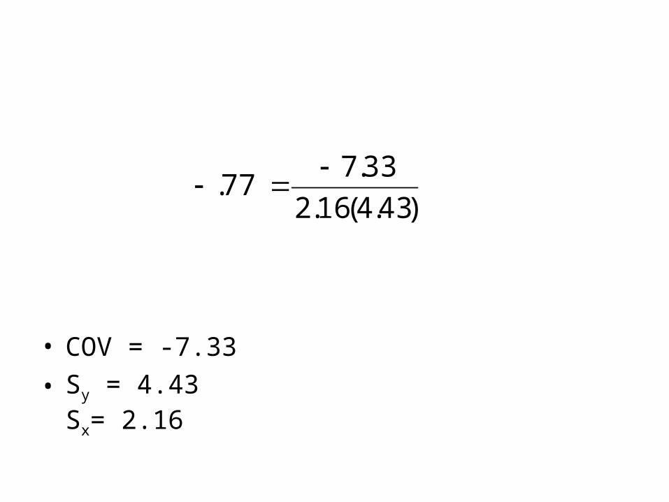
• COV = -7.33
• Sy = 4.43Sx= 2.16
)43.4(16.2
33.777.
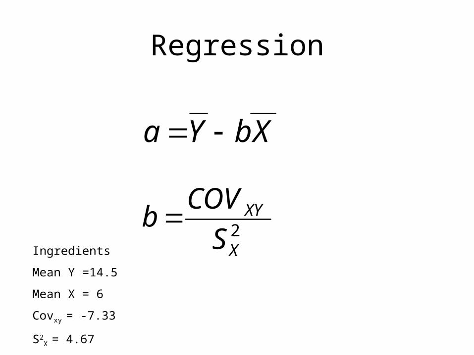
Regression
XbYa
2X
XY
S
COVb
Ingredients
Mean Y =14.5
Mean X = 6
Covxy = -7.33
S2X = 4.67

Regression
6)57.1(5.1492.23 a
67.4
33.757.1
b
Ingredients
Mean Y =14.5
Mean X = 6
Covxy = -7.33
S2X = 4.67
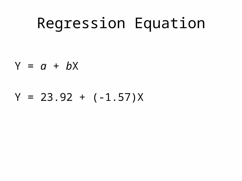
Regression Equation
Y = a + bX
Y = 23.92 + (-1.57)X
0
2
4
6
8
10
12
1 2 3 4 5 6 7 8 9 10
Happiness
Aggression
.
.
..
10
12
14
16
18
20
22
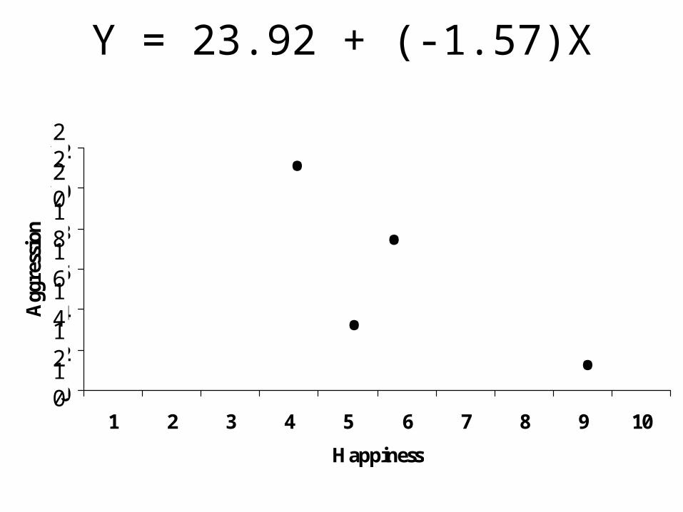
Y = 23.92 + (-1.57)X
0
2
4
6
8
10
12
1 2 3 4 5 6 7 8 9 10
Happiness
Aggression
.
.
..
10
12
14
16
18
20
22
Y = 23.92 + (-1.57)X
.
0
2
4
6
8
10
12
1 2 3 4 5 6 7 8 9 10
Happiness
Aggression
.
.
..
10
12
14
16
18
20
22
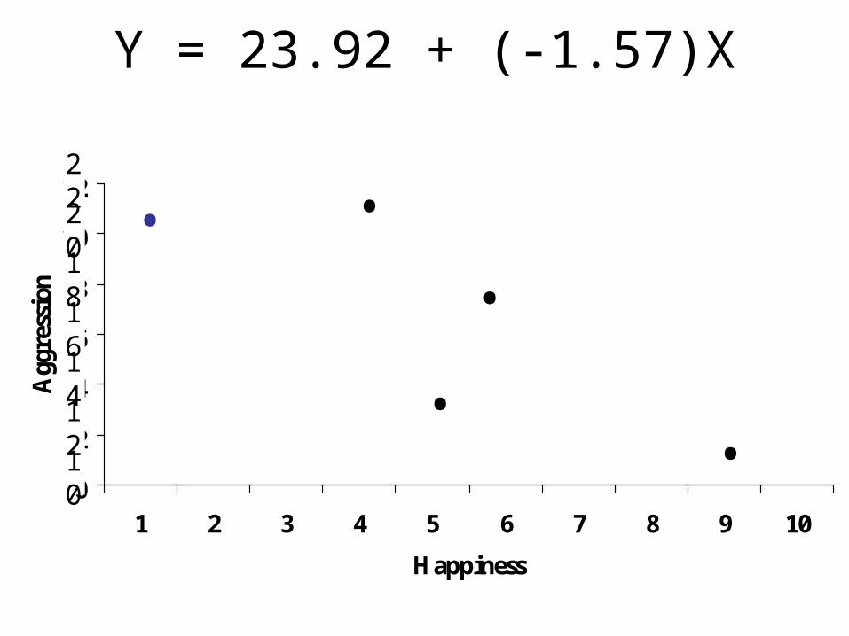
Y = 23.92 + (-1.57)X
.
.

0
2
4
6
8
10
12
1 2 3 4 5 6 7 8 9 10
Happiness
Aggression
.
.
..
10
12
14
16
18
20
22
Y = 23.92 + (-1.57)X
.
.
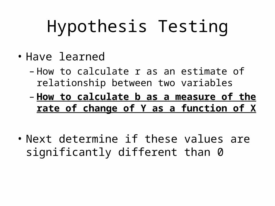
Hypothesis Testing
• Have learned– How to calculate r as an estimate of
relationship between two variables– How to calculate b as a measure of the rate
of change of Y as a function of X
• Next determine if these values are significantly different than 0

Testing b
• The significance test for r and b are equivalent
• If X and Y are related (r), then it must be true that Y varies with X (b).
• Important to learn b significance tests for multiple regression
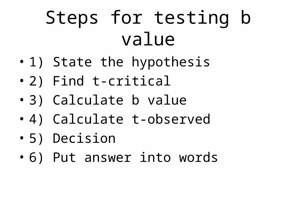
Steps for testing b value
• 1) State the hypothesis
• 2) Find t-critical
• 3) Calculate b value
• 4) Calculate t-observed
• 5) Decision
• 6) Put answer into words
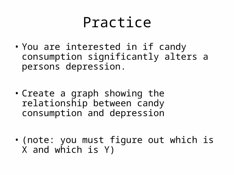
Practice
• You are interested in if candy consumption significantly alters a persons depression.
• Create a graph showing the relationship between candy consumption and depression
• (note: you must figure out which is X and which is Y)
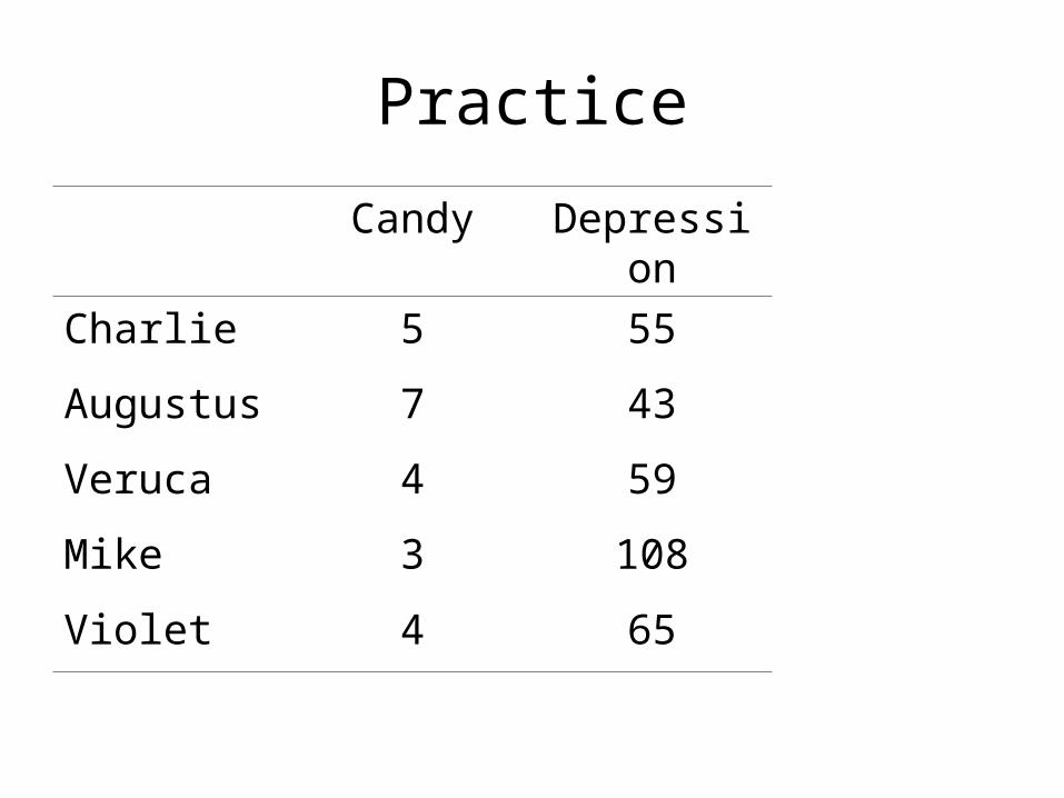
Practice
Candy Depression
Charlie 5 55
Augustus 7 43
Veruca 4 59
Mike 3 108
Violet 4 65
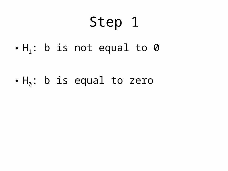
Step 1
• H1: b is not equal to 0
• H0: b is equal to zero
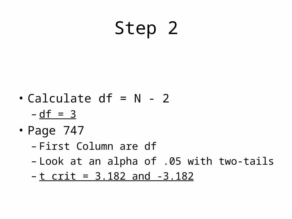
Step 2
• Calculate df = N - 2– df = 3
• Page 747– First Column are df– Look at an alpha of .05 with two-tails– t crit = 3.182 and -3.182
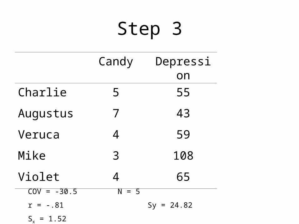
Step 3
Candy Depression
Charlie 5 55
Augustus 7 43
Veruca 4 59
Mike 3 108
Violet 4 65
COV = -30.5 N = 5
r = -.81 Sy = 24.82
Sx = 1.52
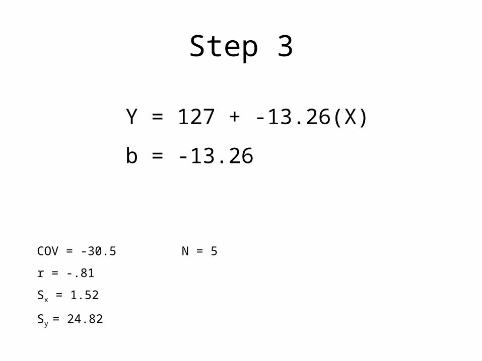
Step 3
COV = -30.5 N = 5
r = -.81
Sx = 1.52
Sy = 24.82
Y = 127 + -13.26(X)
b = -13.26

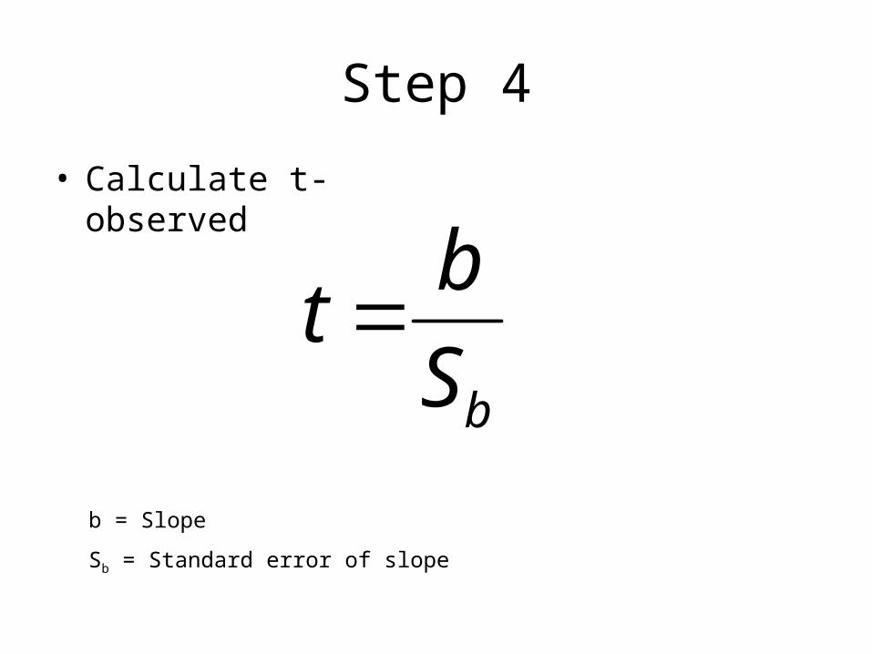
Step 4
• Calculate t-observed
bS
bt
b = Slope
Sb = Standard error of slope

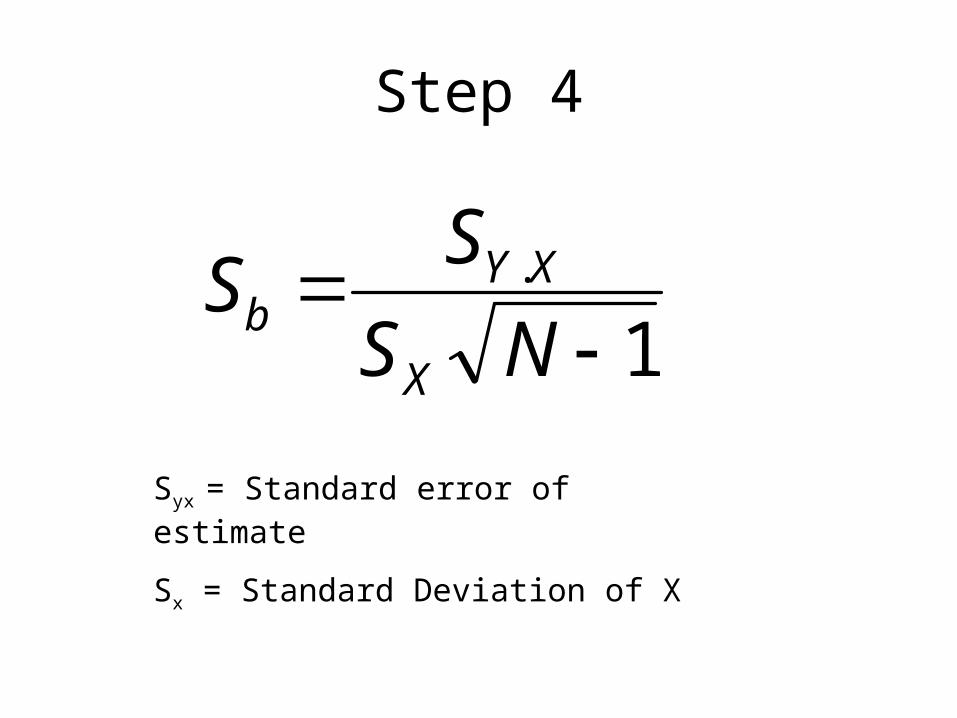
Step 4
1.
NS
SS
X
XYb
Syx = Standard error of estimate
Sx = Standard Deviation of X
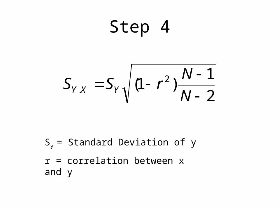
Step 4
2
1)1( 2
.
N
NrSS YXY
Sy = Standard Deviation of y
r = correlation between x and y

Note
2
)ˆ( 2
.
N
YYS XY
0
2
4
6
8
10
12
1 2 3 4 5
Talk
Smile
.
.. ..
Error = 1
Error = -1Error = .5
Error = -.5Error = 0
Error = Y - Y
(Y - Y)2 is minimized
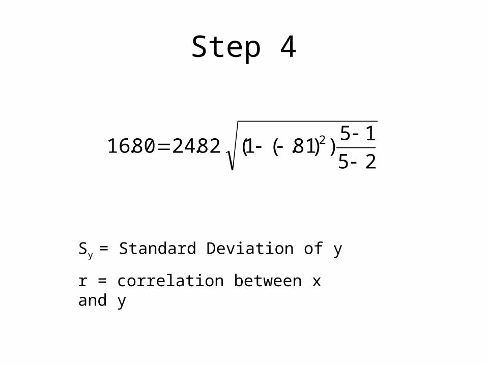
Step 4
25
15))81.(1(82.2480.16 2
Sy = Standard Deviation of y
r = correlation between x and y
Step 4
1.
NS
SS
X
XYb
Syx = Standard error of estimate
Sx = Standard Deviation of X
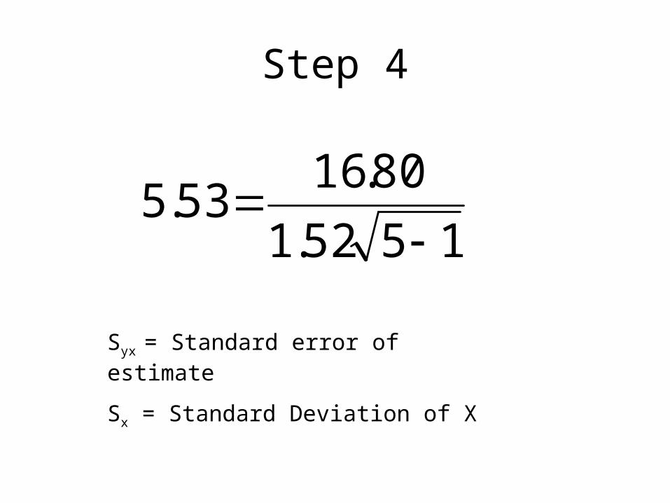
Step 4
1552.1
80.1653.5
Syx = Standard error of estimate
Sx = Standard Deviation of X
Step 4
• Calculate t-observed
bS
bt
b = Slope
Sb = Standard error of slope
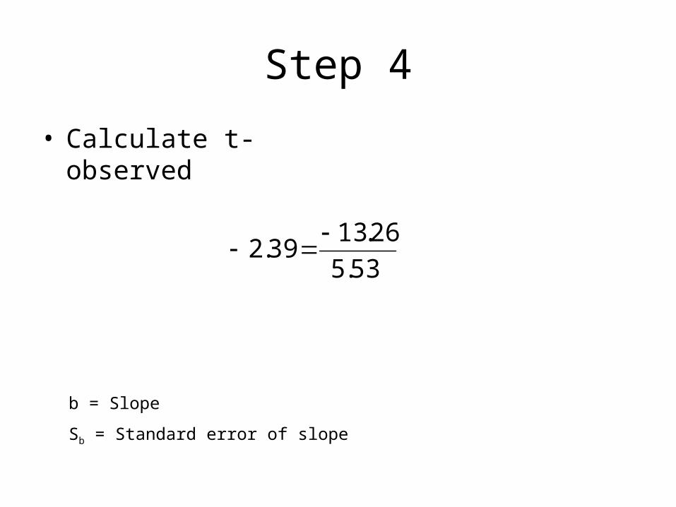
Step 4
• Calculate t-observed
53.5
26.1339.2
b = Slope
Sb = Standard error of slope

Step 4
• Note: same value at t-observed for r
2)81.(1
2581.39.2

Step 5
• If tobs falls in the critical region:
– Reject H0, and accept H1
• If tobs does not fall in the critical region:
– Fail to reject H0
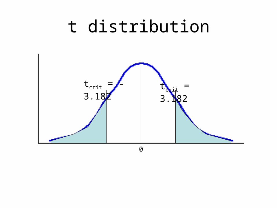
t distribution
tcrit = 3.182tcrit = -3.182
0
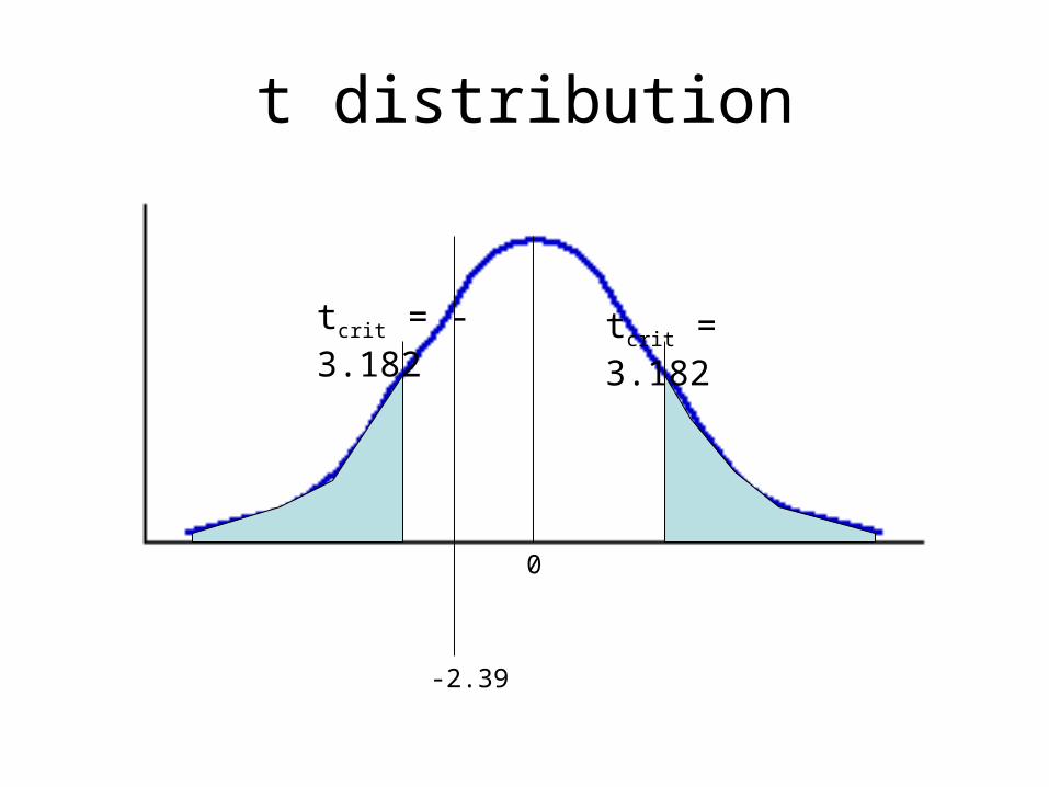
t distribution
tcrit = 3.182tcrit = -3.182
0
-2.39
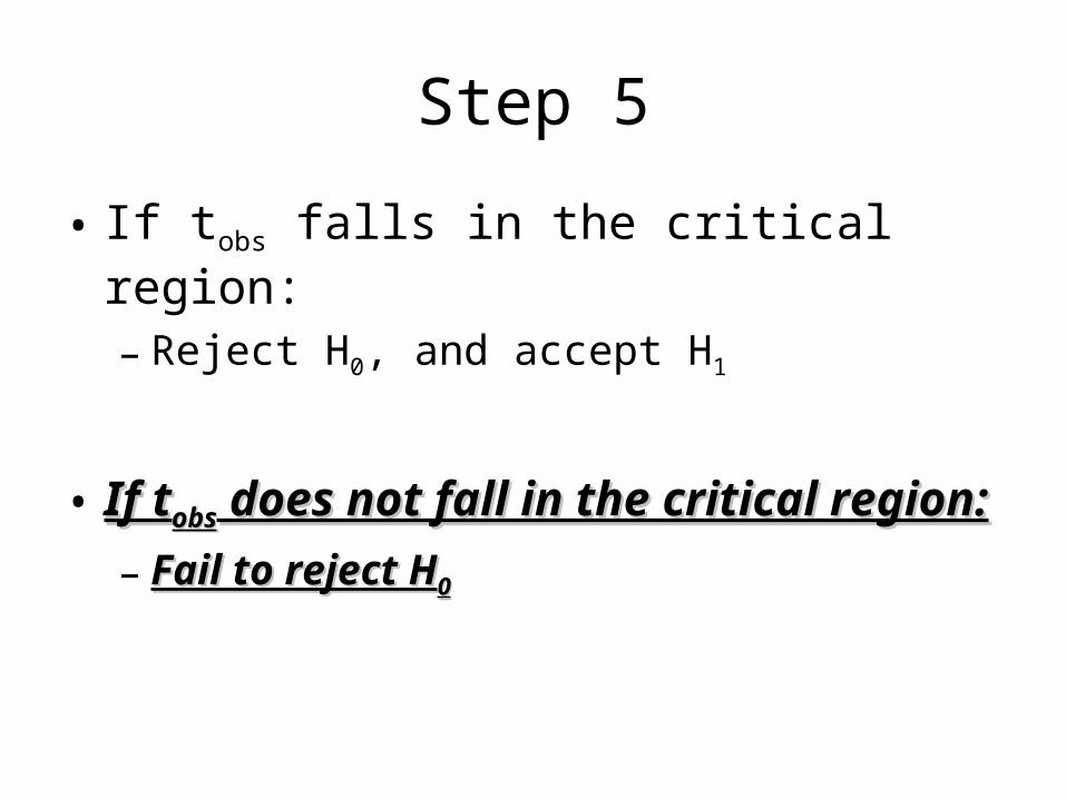
Step 5
• If tobs falls in the critical region:
– Reject H0, and accept H1
• If tIf tobsobs does not fall in the critical region: does not fall in the critical region:
– Fail to reject HFail to reject H00
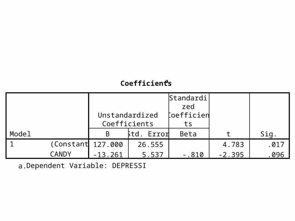
127.000 26.555 4.783 .017
-13.261 5.537 -.810 -2.395 .096
(Constant)
CANDY
Model1
B Std. Error
UnstandardizedCoefficients
Beta
Standardized
Coefficients
t Sig.
Coefficientsa
Dependent Variable: DEPRESSIa.

Practice

Practice
• Page 288
• 9.18
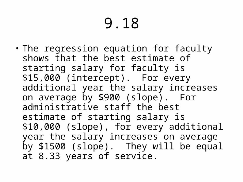
9.18
• The regression equation for faculty shows that the best estimate of starting salary for faculty is $15,000 (intercept). For every additional year the salary increases on average by $900 (slope). For administrative staff the best estimate of starting salary is $10,000 (slope), for every additional year the salary increases on average by $1500 (slope). They will be equal at 8.33 years of service.

Practice
• Page 290
• 9.23
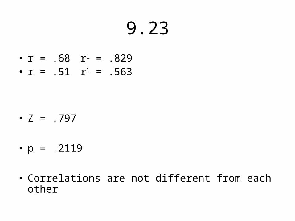
9.23
• r = .68 r1 = .829• r = .51 r1 = .563
• Z = .797
• p = .2119
• Correlations are not different from each other

Discuss
• 9.38
SPSS Problem #3Due March 8th
• Page 287– 9.2– 9.3
– 9.10 and create a graph by hand