Practical Session Instructions

Soil Moisture Retrieval

Prof. Bob Su & M.Sc. Lichun Wang ITC, The Netherlands

(July 2013)

Practical on analysis of soil moisture products Objectives:

• To retrieve the soil moisture using the ITC retrieval model (an example of using METOP ASCAT L1B data).

• To get familiar with soil moisture product retrieved from AMSR-E data. • To get familiar with EUMETSAT soil moisture product retrieved from ASCAT L2

data. • To get familiar with ITC merged AMSR-E and ASCAT L2 soil moisture data. • To get familiar with the SMOS soil moisture products. • To compare the soil moisture products.

Data sets

a) Data sets needed to retrieve the soil moisture using ITC retrieval model - ASCAT L1B files (ASCA_SZR_1B_M02*.nat, native ASCAT format) from July

2008.

- A global land cover map retrieved from the ecoclimap project (landcover.mpr). - A global percentage of sand map retrieved from FAO (1988) soil texture database

(sand.mpr). - A percentage of clay map retrieved from FAO (1988) soil texture database

(clay.mpr) - Leaf area index map obtained from MODIS leaf area index 8-day global 1km

product, temporal coverage 2008-July-03 to 2008-July-10 (LAI.mpr) - Spatial resolution (all maps above): 0.25 degree These files are located in the directory: ASCATL1B b) Soil moisture product retrieved using ITC retrieval model - An image list containing 31 ILWIS maps (unit: cm3/cm3), one for each day

07/01/2008 to 07/31/2008) with global coverage and 0.25 degree spatial resolution. Located in the folder of SM_ITC.

c) Soil moisture product retrieved from ASCAT L2 product

- An image list containing 31 ILWIS maps (unit: cm3/cm3), one for each day 07/01/2008 to 07/31/2008) with global coverage and 0.25 degree spatial resolution. Located in the folder of SM_ASCATL2.

d) Soil moisture product retrieved from AMSR-E - An image list containing 31 ILWIS maps (unit: cm3/cm3), one for each day

07/01/2008 to 07/31/2008) with global coverage and 0.25 degree spatial resolution. Training data is located in the folder of SM_AMSR.

e) ITC Merged AMSR-E and ASCAT L2 soil moisture data - Soil moisture by merging of AMSR-E and ASCAT L2 products - Spatial coverage: China- Tibetan Plateau - Coordinates of the corners: NW Lat 54°N Lon 73°E and SE Lat 20°N Lon 133°E - Grid size 240x136 pixels - Temporal coverage: 07/01/2008 to 07/31/2008 - Temporal resolution: daily average - Spatial resolution: 0.25°

- Format: geotiff images - Note that for the pixels, in which both ASCAT data and AMSR-E data are

available, there is a merging between them. For those pixels with only one product (e.g. either AMSR-E of ASCAT data) available, there is no further data processing needed other than the bias correction, before being combined into the merged product.

f) Soil moisture and Ocean Salinity (SMOS) Soil moisture product - Two SMOS Level 2 (L2) soil moisture products (reprocessed data), over Maqu

site of Tibet, China, are provided for this training. Training data is Located in the folder of SM_SMOS.

Exercise steps:

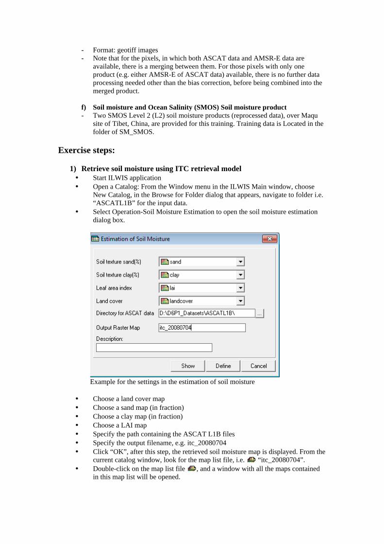
1) Retrieve soil moisture using ITC retrieval model • Start ILWIS application • Open a Catalog: From the Window menu in the ILWIS Main window, choose

New Catalog, in the Browse for Folder dialog that appears, navigate to folder i.e. “ASCATL1B” for the input data.

• Select Operation-Soil Moisture Estimation to open the soil moisture estimation dialog box.

Example for the settings in the estimation of soil moisture

• Choose a land cover map • Choose a sand map (in fraction) • Choose a clay map (in fraction) • Choose a LAI map • Specify the path containing the ASCAT L1B files • Specify the output filename, e.g. itc_20080704 • Click “OK”, after this step, the retrieved soil moisture map is displayed. From the

current catalog window, look for the map list file, i.e. “itc_20080704”. • Double-click on the map list file , and a window with all the maps contained

in this map list will be opened.

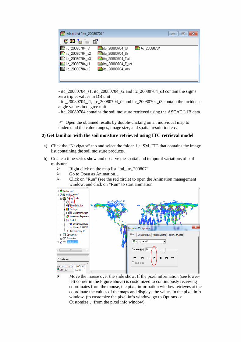
- itc_20080704_s1, itc_20080704_s2 and itc_20080704_s3 contain the sigma zero triplet values in DB unit - itc_20080704_t1, itc_20080704_t2 and itc_20080704_t3 contain the incidence angle values in degree unit - itc_20080704 contains the soil moisture retrieved using the ASCAT L1B data.

Open the obtained results by double-clicking on an individual map to understand the value ranges, image size, and spatial resolution etc.

2) Get familiar with the soil moisture retrieved using ITC retrieval model

a) Click the “Navigator” tab and select the folder .i.e. SM_ITC that contains the image list containing the soil moisture products.

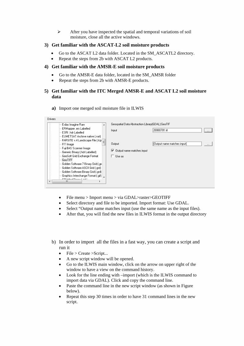
b) Create a time series show and observe the spatial and temporal variations of soil moisture. Right click on the map list “ml_itc_200807”. Go to Open as Animation… Click on “Run” (see the red circle) to open the Animation management

window, and click on “Run” to start animation.

Move the mouse over the slide show. If the pixel information (see lower-

left corner in the Figure above) is customized to continuously receiving coordinates from the mouse, the pixel information window retrieves at the coordinate the values of the maps and displays the values in the pixel info window. (to customize the pixel info window, go to Options -> Customize… from the pixel info window)

After you have inspected the spatial and temporal variations of soil moisture, close all the active windows.

3) Get familiar with the ASCAT-L2 soil moisture products • Go to the ASCAT L2 data folder. Located in the SM_ASCATL2 directory. • Repeat the steps from 2b with ASCAT L2 products.

4) Get familiar with the AMSR-E soil moisture products • Go to the AMSR-E data folder, located in the SM_AMSR folder • Repeat the steps from 2b with AMSR-E products.

5) Get familiar with the ITC Merged AMSR-E and ASCAT L2 soil moisture

data

a) Import one merged soil moisture file in ILWIS

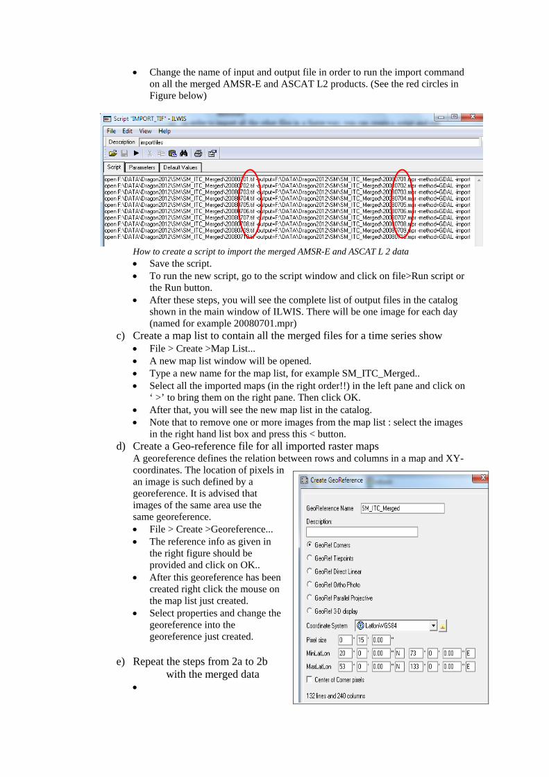
• File menu > Import menu > via GDAL>raster>GEOTIFF • Select directory and file to be imported. Import format: Use GDAL. • Select “Output name matches input (use the same name as the input files). • After that, you will find the new files in ILWIS format in the output directory

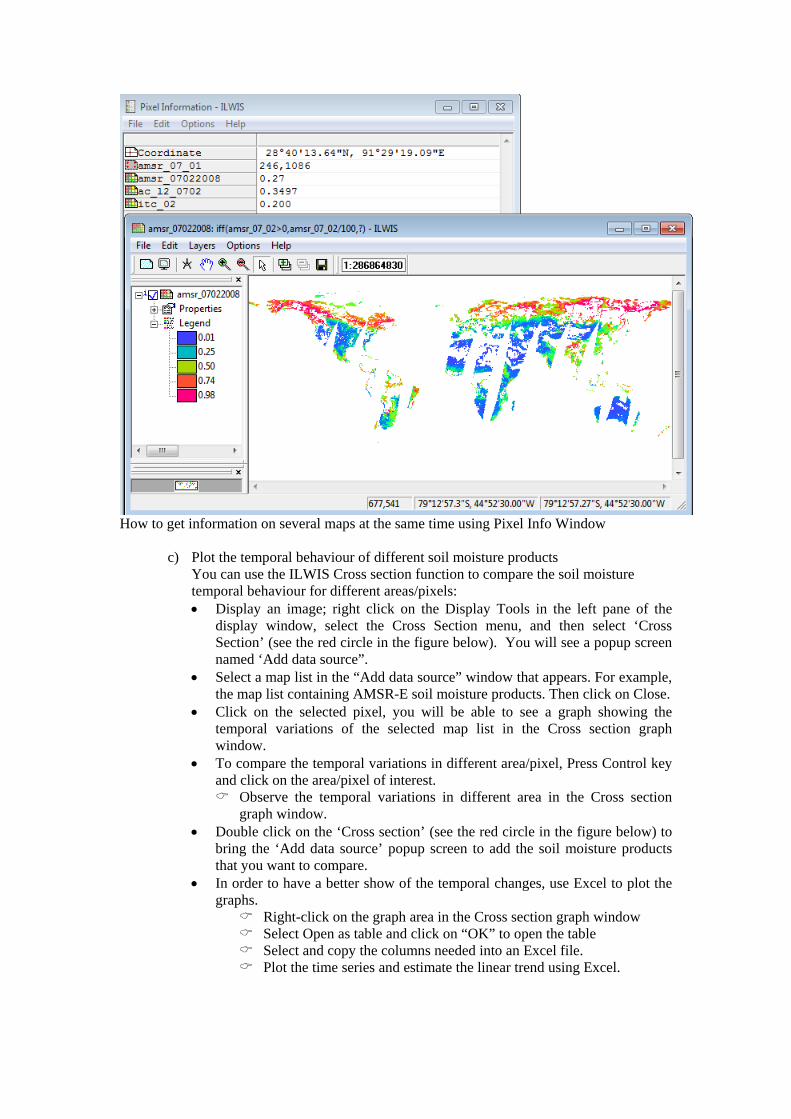
b) In order to import all the files in a fast way, you can create a script and run it • File > Create >Script... • A new script window will be opened. • Go to the ILWIS main window, click on the arrow on upper right of the

window to have a view on the command history. • Look for the line ending with –import (which is the ILWIS command to

import data via GDAL). Click and copy the command line. • Paste the command line in the new script window (as shown in Figure

below). • Repeat this step 30 times in order to have 31 command lines in the new

script.

• Change the name of input and output file in order to run the import command on all the merged AMSR-E and ASCAT L2 products. (See the red circles in Figure below)

How to create a script to import the merged AMSR-E and ASCAT L 2 data • Save the script. • To run the new script, go to the script window and click on file>Run script or

the Run button. • After these steps, you will see the complete list of output files in the catalog

shown in the main window of ILWIS. There will be one image for each day (named for example 20080701.mpr)

c) Create a map list to contain all the merged files for a time series show • File > Create >Map List... • A new map list window will be opened. • Type a new name for the map list, for example SM_ITC_Merged.. • Select all the imported maps (in the right order!!) in the left pane and click on

‘ >’ to bring them on the right pane. Then click OK. • After that, you will see the new map list in the catalog. • Note that to remove one or more images from the map list : select the images

in the right hand list box and press this < button. d) Create a Geo-reference file for all imported raster maps

A georeference defines the relation between rows and columns in a map and XY-coordinates. The location of pixels in an image is such defined by a georeference. It is advised that images of the same area use the same georeference. • File > Create >Georeference... • The reference info as given in

the right figure should be provided and click on OK..

• After this georeference has been created right click the mouse on the map list just created.

• Select properties and change the georeference into the georeference just created.

e) Repeat the steps from 2a to 2b

with the merged data •

6) Compare the soil moisture products

a) Compare the histograms • From the ITC-Model catalog window, double-click on the map list

“ml_itc_200807” and a window with all the bands in this list will be opened. • From the ASCAT-L2 catalog window, double click on the map list

“ml_ASCAT_200807” and a window with all the bands in this list will be opened.

• From the AMSR catalog window, double-click on the map list “ml_amsr_200807” and a window with all the bands in this list will be opened.

• Showing the histograms of the same bands from these products. For example, the histogram of July 4th 2008 of the ITC-model, ASCAT-L2, and AMSR products. To do this, double-click on the band “itc_04” from map list “ml_itc_200807” and then go to Statistics -> Histograms… then click on Show.

• Double-click on the “ac_l2_0704” band from the map list “ml_amsr_200807” and then go to Statistics -> Histograms… then click on Show.

• Double-click on the band “amsr_07_04” from map list “ml_amsr_200807” and then go to Statistics -> Histograms… then click on Show.

• Comparing the histograms Do you see a significant difference between the histograms?

• Please do the histogram comparison for soil products of different date.

b) Compare the soil moisture temporal behaviour using pixel info window • In the map list “ml_amsr_072008 window”, double-click on the first map i.e.

“amsr_07012008” to show the image. In the Pixel Information window (left corner of the map window), deselect the option “Continuous”.

• In the map list “ml_ascat_200807” window, select and drag the first band “ac_l2_0701” to the Pixel Information Window.

• In the map list “ml_itc_200807” window, select and drag the band “itc_01” to the Pixel Information Window.

• In the ITC merged map list window, select and drag the band ‘20080701’ to the pixel info window.

• Choose an area where to compare the temporal behaviour of the four products. For example you can choose the centre of Naqu site, Tibet, China (31° 21’ N, 91° 52’ E). At the bottom right of the map display window, you can read the geographic coordinates of the pixel. Click on the selected pixel, you will be able to read the pixel values of the three maps in the Pixel Info Window.

Repeat the comparison over different pixels.

How to get information on several maps at the same time using Pixel Info Window

c) Plot the temporal behaviour of different soil moisture products You can use the ILWIS Cross section function to compare the soil moisture temporal behaviour for different areas/pixels: • Display an image; right click on the Display Tools in the left pane of the

display window, select the Cross Section menu, and then select ‘Cross Section’ (see the red circle in the figure below). You will see a popup screen named ‘Add data source”.

• Select a map list in the “Add data source” window that appears. For example, the map list containing AMSR-E soil moisture products. Then click on Close.

• Click on the selected pixel, you will be able to see a graph showing the temporal variations of the selected map list in the Cross section graph window.

• To compare the temporal variations in different area/pixel, Press Control key and click on the area/pixel of interest. Observe the temporal variations in different area in the Cross section

graph window. • Double click on the ‘Cross section’ (see the red circle in the figure below) to

bring the ‘Add data source’ popup screen to add the soil moisture products that you want to compare.

• In order to have a better show of the temporal changes, use Excel to plot the graphs.

Right-click on the graph area in the Cross section graph window Select Open as table and click on “OK” to open the table Select and copy the columns needed into an Excel file. Plot the time series and estimate the linear trend using Excel.

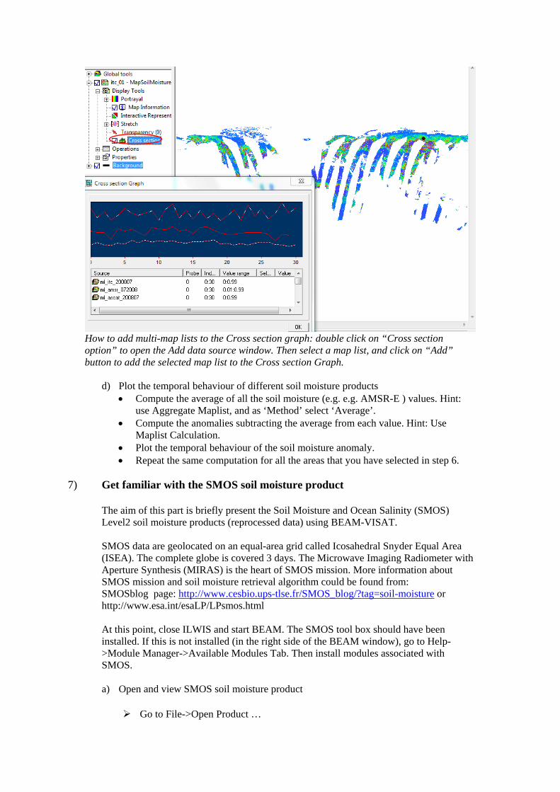
How to add multi-map lists to the Cross section graph: double click on “Cross section option” to open the Add data source window. Then select a map list, and click on “Add” button to add the selected map list to the Cross section Graph.

d) Plot the temporal behaviour of different soil moisture products • Compute the average of all the soil moisture (e.g. e.g. AMSR-E ) values. Hint:

use Aggregate Maplist, and as ‘Method’ select ‘Average’. • Compute the anomalies subtracting the average from each value. Hint: Use

Maplist Calculation. • Plot the temporal behaviour of the soil moisture anomaly. • Repeat the same computation for all the areas that you have selected in step 6.

7) Get familiar with the SMOS soil moisture product

The aim of this part is briefly present the Soil Moisture and Ocean Salinity (SMOS) Level2 soil moisture products (reprocessed data) using BEAM-VISAT. SMOS data are geolocated on an equal-area grid called Icosahedral Snyder Equal Area (ISEA). The complete globe is covered 3 days. The Microwave Imaging Radiometer with Aperture Synthesis (MIRAS) is the heart of SMOS mission. More information about SMOS mission and soil moisture retrieval algorithm could be found from: SMOSblog page: http://www.cesbio.ups-tlse.fr/SMOS_blog/?tag=soil-moisture or http://www.esa.int/esaLP/LPsmos.html At this point, close ILWIS and start BEAM. The SMOS tool box should have been installed. If this is not installed (in the right side of the BEAM window), go to Help->Module Manager->Available Modules Tab. Then install modules associated with SMOS. a) Open and view SMOS soil moisture product

Go to File->Open Product …

From the file selection dialog window, navigate to the folder i.e. “SM_SMOS” with SMOS soil moisture products.

Double-click on the first data set from the dialog box, select the DBL file that appears, and then click on the “Open Product” button to return to the BEAM window.

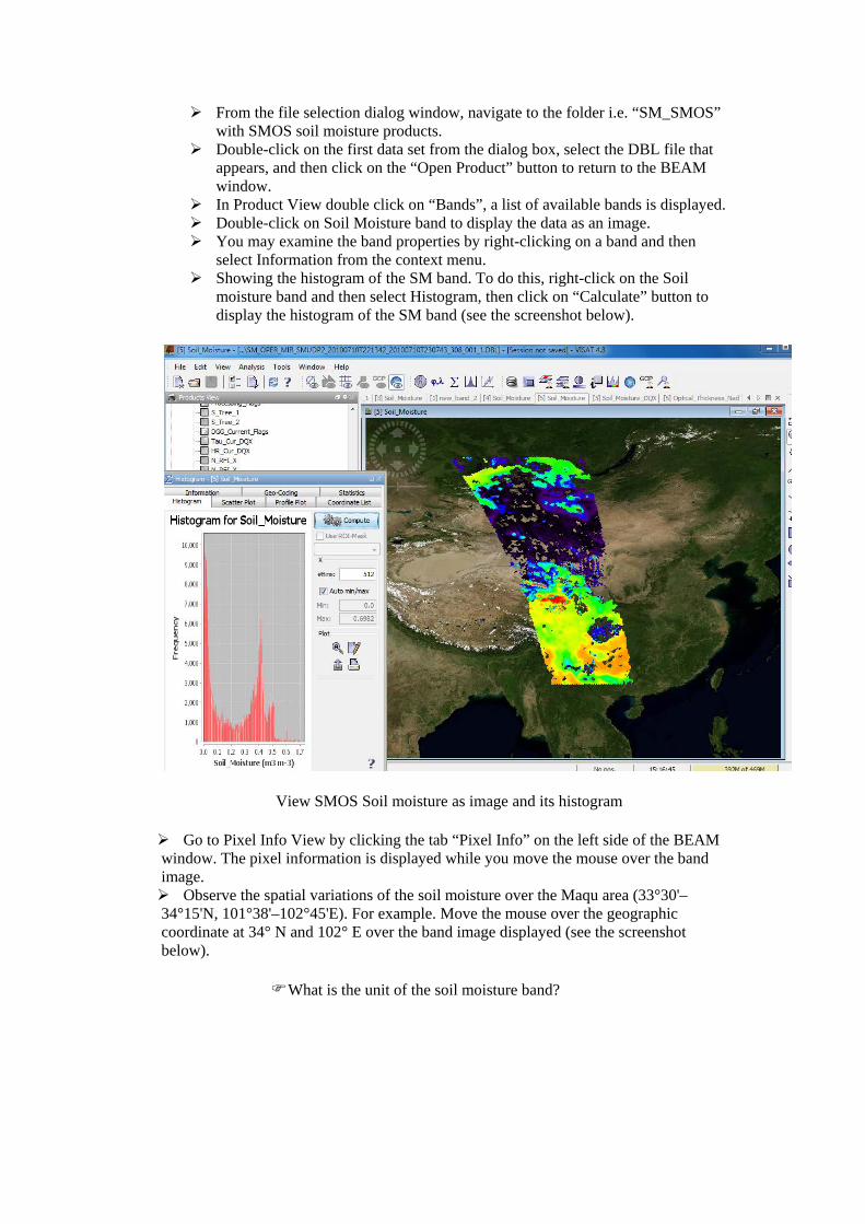
In Product View double click on “Bands”, a list of available bands is displayed. Double-click on Soil Moisture band to display the data as an image. You may examine the band properties by right-clicking on a band and then

select Information from the context menu. Showing the histogram of the SM band. To do this, right-click on the Soil

moisture band and then select Histogram, then click on “Calculate” button to display the histogram of the SM band (see the screenshot below).

View SMOS Soil moisture as image and its histogram

Go to Pixel Info View by clicking the tab “Pixel Info” on the left side of the BEAM window. The pixel information is displayed while you move the mouse over the band image. Observe the spatial variations of the soil moisture over the Maqu area (33°30'–34°15'N, 101°38'–102°45'E). For example. Move the mouse over the geographic coordinate at 34° N and 102° E over the band image displayed (see the screenshot below).

What is the unit of the soil moisture band?

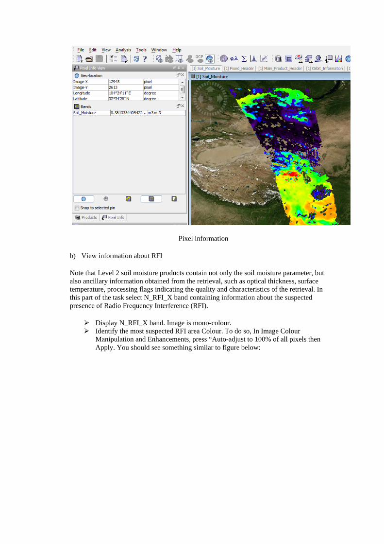
Pixel information

b) View information about RFI

Note that Level 2 soil moisture products contain not only the soil moisture parameter, but also ancillary information obtained from the retrieval, such as optical thickness, surface temperature, processing flags indicating the quality and characteristics of the retrieval. In this part of the task select N_RFI_X band containing information about the suspected presence of Radio Frequency Interference (RFI).

Display N_RFI_X band. Image is mono-colour. Identify the most suspected RFI area Colour. To do so, In Image Colour

Manipulation and Enhancements, press “Auto-adjust to 100% of all pixels then Apply. You should see something similar to figure below:

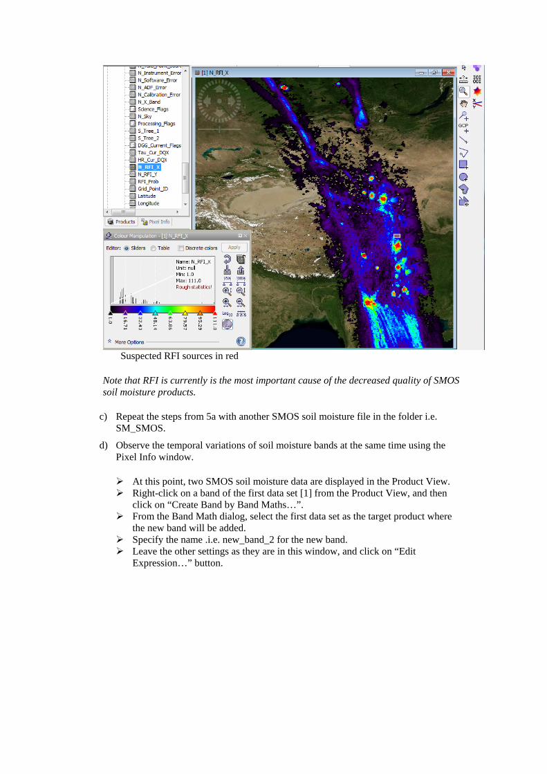
Suspected RFI sources in red

Note that RFI is currently is the most important cause of the decreased quality of SMOS soil moisture products.

c) Repeat the steps from 5a with another SMOS soil moisture file in the folder i.e. SM_SMOS.

d) Observe the temporal variations of soil moisture bands at the same time using the Pixel Info window.

At this point, two SMOS soil moisture data are displayed in the Product View. Right-click on a band of the first data set [1] from the Product View, and then

click on “Create Band by Band Maths…”. From the Band Math dialog, select the first data set as the target product where

the new band will be added. Specify the name .i.e. new_band_2 for the new band. Leave the other settings as they are in this window, and click on “Edit

Expression…” button.

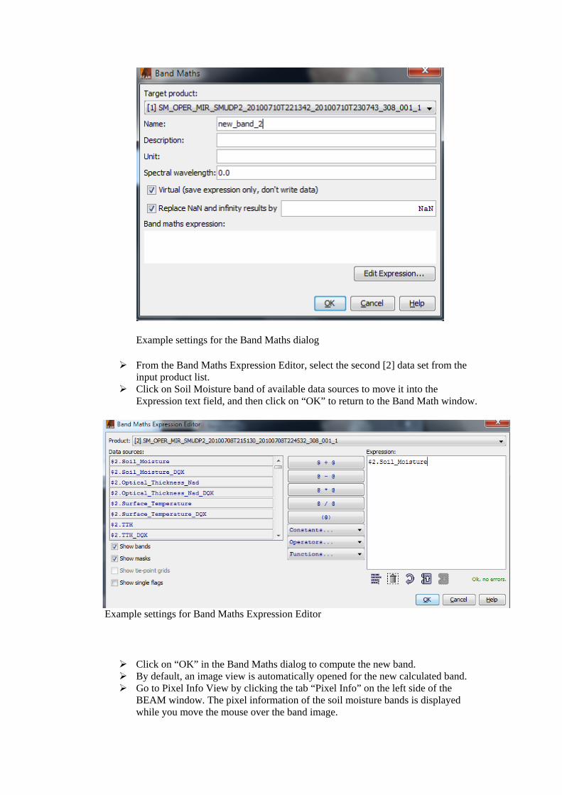
Example settings for the Band Maths dialog

From the Band Maths Expression Editor, select the second [2] data set from the input product list.

Click on Soil Moisture band of available data sources to move it into the Expression text field, and then click on “OK” to return to the Band Math window.

Example settings for Band Maths Expression Editor

Click on “OK” in the Band Maths dialog to compute the new band. By default, an image view is automatically opened for the new calculated band. Go to Pixel Info View by clicking the tab “Pixel Info” on the left side of the

BEAM window. The pixel information of the soil moisture bands is displayed while you move the mouse over the band image.

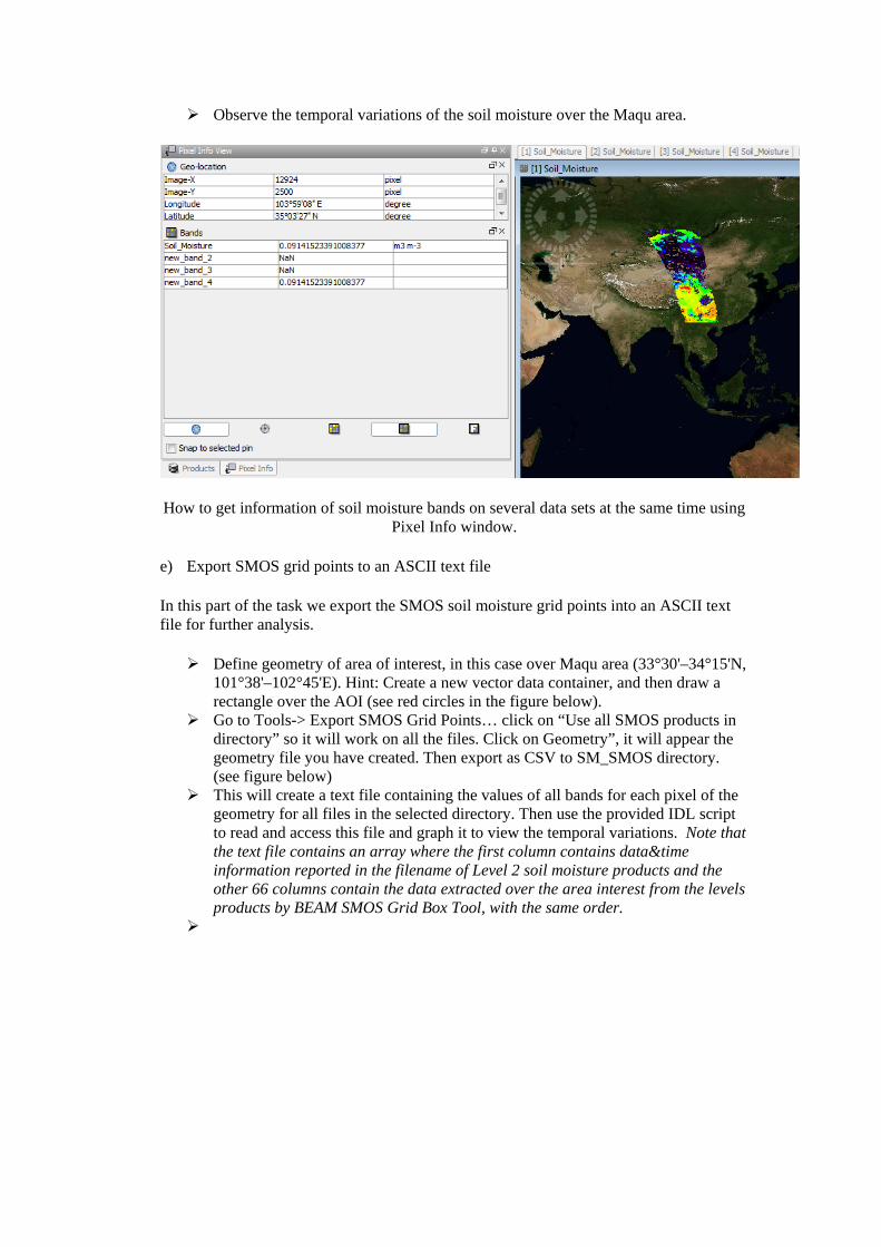
Observe the temporal variations of the soil moisture over the Maqu area.

How to get information of soil moisture bands on several data sets at the same time using Pixel Info window.

e) Export SMOS grid points to an ASCII text file

In this part of the task we export the SMOS soil moisture grid points into an ASCII text file for further analysis.

Define geometry of area of interest, in this case over Maqu area (33°30'–34°15'N, 101°38'–102°45'E). Hint: Create a new vector data container, and then draw a rectangle over the AOI (see red circles in the figure below).

Go to Tools-> Export SMOS Grid Points… click on “Use all SMOS products in directory” so it will work on all the files. Click on Geometry”, it will appear the geometry file you have created. Then export as CSV to SM_SMOS directory. (see figure below)

This will create a text file containing the values of all bands for each pixel of the geometry for all files in the selected directory. Then use the provided IDL script to read and access this file and graph it to view the temporal variations. Note that the text file contains an array where the first column contains data&time information reported in the filename of Level 2 soil moisture products and the other 66 columns contain the data extracted over the area interest from the levels products by BEAM SMOS Grid Box Tool, with the same order.

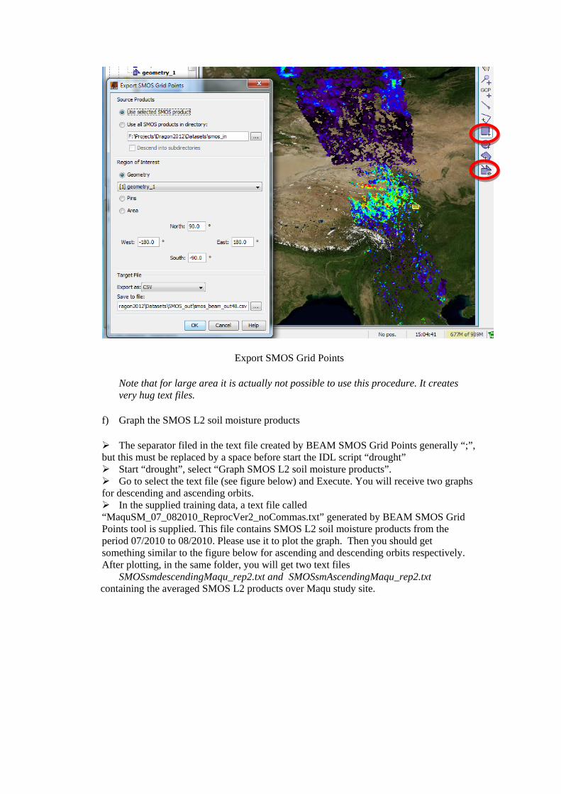
Export SMOS Grid Points

Note that for large area it is actually not possible to use this procedure. It creates very hug text files.

f) Graph the SMOS L2 soil moisture products

The separator filed in the text file created by BEAM SMOS Grid Points generally “;”, but this must be replaced by a space before start the IDL script “drought” Start “drought”, select “Graph SMOS L2 soil moisture products”. Go to select the text file (see figure below) and Execute. You will receive two graphs for descending and ascending orbits. In the supplied training data, a text file called “MaquSM_07_082010_ReprocVer2_noCommas.txt” generated by BEAM SMOS Grid Points tool is supplied. This file contains SMOS L2 soil moisture products from the period 07/2010 to 08/2010. Please use it to plot the graph. Then you should get something similar to the figure below for ascending and descending orbits respectively. After plotting, in the same folder, you will get two text files SMOSsmdescendingMaqu_rep2.txt and SMOSsmAscendingMaqu_rep2.txt

containing the averaged SMOS L2 products over Maqu study site.

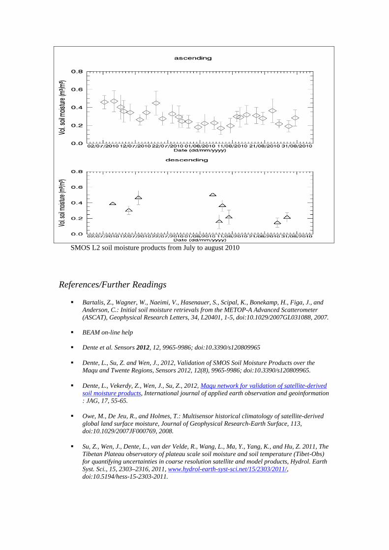
SMOS L2 soil moisture products from July to august 2010

References/Further Readings

Bartalis, Z., Wagner, W., Naeimi, V., Hasenauer, S., Scipal, K., Bonekamp, H., Figa, J., and Anderson, C.: Initial soil moisture retrievals from the METOP-A Advanced Scatterometer (ASCAT), Geophysical Research Letters, 34, L20401, 1-5, doi:10.1029/2007GL031088, 2007.

BEAM on-line help

Dente et al. Sensors 2012, 12, 9965-9986; doi:10.3390/s120809965

Dente, L., Su, Z. and Wen, J., 2012, Validation of SMOS Soil Moisture Products over the Maqu and Twente Regions, Sensors 2012, 12(8), 9965-9986; doi:10.3390/s120809965.

Dente, L., Vekerdy, Z., Wen, J., Su, Z., 2012, Maqu network for validation of satellite-derived soil moisture products, International journal of applied earth observation and geoinformation : JAG, 17, 55-65.

Owe, M., De Jeu, R., and Holmes, T.: Multisensor historical climatology of satellite-derived global land surface moisture, Journal of Geophysical Research-Earth Surface, 113, doi:10.1029/2007JF000769, 2008.

Su, Z., Wen, J., Dente, L., van der Velde, R., Wang, L., Ma, Y., Yang, K., and Hu, Z. 2011, The Tibetan Plateau observatory of plateau scale soil moisture and soil temperature (Tibet-Obs) for quantifying uncertainties in coarse resolution satellite and model products, Hydrol. Earth Syst. Sci., 15, 2303–2316, 2011, www.hydrol-earth-syst-sci.net/15/2303/2011/, doi:10.5194/hess-15-2303-2011.

Wagner, W., Lemoine, G., and Rott, H.: A method for estimating soil moisture from ERS scatterometer and soil data. Remote Sensing of Environment, 70, 191-207, 1999.

Wen, J., Z. Su, 2003, A Method for Estimating Relative Soil Moisture with ESA Wind Scatterometer Data, Geophysical Research Letters, 30 (7), 1397, doi:10.1029/ 2002GL016557.

Wen, J., Z. Su, 2003, Estimation of soil moisture from ESA Wind-scatterometer data, Physics and Chemistry of the Earth, 28(1-3), 53-61.

Wen, J., Z. Su, 2004, An analytical algorithm for the determination of vegetation Leaf Area Index from TRMM/TMI data, International Journal of Remote Sensing, 25(6), 1223–1234.

Wen, J., Z. Su, Y. Ma, 2003, Determination of Land Surface Temperature and Soil Moisture from TRMM/TMI Remote Sensing Data, Journal of Geophysical Research, 108(D2), 10.1029/2002JD002176.