Embed Size (px)
Citation preview
NASA CR- 1129
JPRACTICAL RELIABILITY
Volume IV - Prediction
Distribution of this report is provided in the interest of
information exchange. Responsibility for the contentsresides in the author or organization that prepared it.
Prepared under Contract No. NASw-1448 byRESEARCH TRIANGLE INSTITUTE
Research Triangle Park, N.C.
for
NATIONAL AERONAUTICS AND SPACE ADMINISTRATION
For sale by the Clearinghouse for Federal Scientific and Technical InformationSpringfield, Virginia 22151 - CFSTI price $3.00
https://ntrs.nasa.gov/search.jsp?R=19680022507 2018-07-13T21:41:21+00:00Z

i

FOI_WORD
The typical few-of-a-kind nature of NASA systems has made reliability a premi_n
en on the initial items delivered in a program. Reliability defined and treated on
basis of percentage of items operating successfully has much less meaning than
aen larger sample sizes are available as in military and commercial products. Relia-
ility thus becomes based more on engineering confidence that the item will work as
intended. The key to reliability is thus good englneerlng--deslgning reliability
into the system and engineering to prevent degradation of the deslgned-in reliability
from fabrication, testing and operation.
The PRACTICAL RELIABILITY series of reports is addressed to the typical engineer
to aid his comprehension of practical problems in engineering for reliability. In
these reports the intent is to present fundamental concepts on a particular subject in
an interesting, mainly narrative form and make the reader aware of practical problems
in applying them. There is little emphasis on describing procedures and how to
implement them. Thus there is liberal use of references for both background theory
and cookbook procedures. The present coverage is limited to five subject areas:
Vol. I. - Parameter Variation Analysis describes the techniques for treating
the effect of system parameters on performance, reliability, and other figures-
of-merlt.
Vol. II. - Computation considers the digital computer and where and how it can
be used to aid various reliability tasks.
Vol. III.- Testing describes the basic approaches to testing and emphasizes
the practical considerations and the applications to reliability.
Vol. IV. - Prediction presents mathematical methods and analysis approaches
for reliability prediction and includes some methods not generally covered in
texts and handbooks.
Vol. V. - Parts reviews the processes and procedures required to obtain and
apply parts which will perform their functions adequately.
These reports were prepared by the Research Triangle Institute, Research Triangle
Park, North Carolina 27709 under NASA Contract NASw-1448. The contract was adminis-
tered under the technical direction of the Office of Reliability and Quality
Assurance, NASA Headquarters, Washington, D. C. 20546 with Dr. John E. Condon,
Director, as technical contract monitor. The contract effort was performed Jointly
by personnel from both the Statistics Research and the Engineering and Environmental
Sciences Divisions. Dr. R. M. Burger was technical director with W. S. Thompson
serving as project leader.
iii

This report is Vol. IV - Prediction. This subject has been of interest in
reliability work since the earliest efforts of organized reliability activity. In
these ensuing years much has been written on reliability prediction, but often the
item concentrates on limited facets of the subject. This report synthesizes
reliability prediction, with emphasis on the basics and the scope. C. A. Krohn
selected and organized the contents, and together with A. C. Nelson, Jr. prepared
the material. W. S. Thompson provided helpful comments.
iv
ABSTRACT
Thefeatures andtechniques of reliability prediction are identified andbroughttogether in this report. Theapproachis to:
(a) Bring together scattered material,(b) Present somematerial not in booksor handbooks,(c) Identify several points which have a tendency to be missed,
(d) Present some ideas which may be helpful to others involved in develop-
ment of reliability prediction techniques, and
(e) Express some opinions related to the role of reliability prediction.
Material presented in this report is grouped into four major categories.
Part I is largely qualitative discussion concerned with introduction and perspective.
Contents include discussion and opinions on the role of reliability prediction, on
perspective features_ e.g. program phase and hardware level, on the relation to other
analyses, and on the problems. Part II is concerned with reliability measures or
definitions concerning single items, including data sources. Part III is devoted to
the reliability prediction techniques which are suitable for general use and to
classical reliability models. This material is scattered throughout the references;
the treatment here mainly identifies approaches and relates them, with
reliance on the references. Included for multi-item models are logic, lifetime,
environment and bound-crossing topics. The remaining Part IV is concerned with
concepts related to the detailed treatment of failure modes without independence
assumptions. This is food-for-thought material from the results of research on
reliability prediction techniques. This material in Part IV, in general, is not
suited for widespread application. The Appendix presents a ready-reference on some
basic probability laws and on various probability distributions.

PAG_ BLANK NOT FILMED.pp_ECEDING REPORT PREFACE
In this report the subject of reliability prediction is synthesized. It is
an attempt to "see the forest", but done while keeping both feet on the ground.
Fundamentals are stressed in order to help develop a better understanding of what is
involved. Expanded treatment is given to basic reliability measures, to some points
which have a tendency to be somewhat misunderstood in the literature, and to several
topics which are not covered in existing books and handbooks but where RTI has delved
into them. Other topics are identified and related to one-another.
Reliability prediction as an organized discipline is approximately 15 years
old. There are approximately a dozen books on the subject and approximately the same
number of handbooks. There are many hundreds of reports and papers. Some which
treat the fundamentals will be relied on heavily.
The qualitative discussion of Part I on the scope of reliability prediction is
suitable for any reader - design engineer, manager, reliability generalist, or
reliability analyst. Parts II and III cover mainly conventional and classical
approaches to reliability prediction and Part IV reports on some research on struc-
turing certain detail into a prediction. Parts II, III and IV will not be easy reading
for persons who are not knowledgeable in the mathematics of probability. Of course
perusing these parts will give any reader a flavor of the subject. If a reader
wants to understand the subject he will have to study the material as introduced here
and as elaborated in the references. If he does not know the mathematics of probabilitl
then he will first need to learn its fundamentals. The practicing reliability analyst
should be familiar with most of the contents. For him, perhaps the manner in which
the material is organized, the identification of references, and the results of
research on reliability prediction techniques in Part IV will be of interest.
vii

,
7.
80
9,
TABLE OF CONTENTS (Continued)
Numerical Index Values
6.1
6.2
6.3
6.4
Comprehensive Guide
Reliability Measure Sources
Bound-Crossing Data
Remarks
Part III: Multi-ltem Problems
Logic Models
7.1 Basic Set Operations and Calculus of Probability
7.2 Applications to Various System Configurations
7.3 Conditional Probabilistic Approach
7.4 Models Using Cuts and Paths
7.5 Multi-Phase Mission
7.6 N-State Logic Model
Models Considering Time
8.1 Logic Model Substitution
8.2 Standby and Rope Models
8.3 Additional Approaches
8.4 General Redundancy Model
Environment and Bound-Crossing Problems
9.1 Environment Described Probabilistically
9.2 Stress-Strength Problems
9.3 Functionally Related Variables
Part IV: Refinements of Prediction Models
i0. Catastrophic and Degradation Failures
Ii. A Detailed Prediction Example
12. General Model Development
12.1 Series Situation Model
12.2 Numerical Calculation
12.3 Additional Considerations
13. Concluding Remarks for Part IV
Pase No.
51
51
51
52
52
55
55
60
67
70
74
78
81
81
83
88
90
98
98
99
106
115
i17
124
124
132
135
137
x
PKECEDING PAGE BLANK, NOT FILMED.
TABLE OF CONTENTS
FOREWORD
ABSTRACT
REPORT PREFACE
l,
2.
,
Part I: Perspective
Treating Reliability Quantitatively
i.I NASA Definition of Reliabillty
1.2 Probabillstic Approach
1.3 Role
1.4 Uses
1.5 Accuracy
Prediction and Allied Approaches
2.1 Prediction Techniques
2.2 Prediction Technique Choice
2.3 Related Analyses
Needs and Problems
3.1 People
3.2 Data
3.3 Techniques
.
5,
Part II: Single Item Reliability
Reliability Measures
4.1 Definitions of States and Reliability
4.2 Reliability as Function of Time
4.3 Bathtub Curve
4.4 Consideration of the Environment
4.5 Polsson Processes
4.6 Reliability Measures for Repaired Items
4.7 Reliability Measures for Replaced Items
4.8 Bathtub Curve for Repaired Items
Bound-Crossing
5.1
5.2
5.3
5.4
Fundamentals
Fixed Bounds
Stress-Strength Model (Bound Distribution)
Time Dependency
Page No.
ill
V
vii
2
2
2
3
3
3
5
5
8
9
14
14
15
16
18
18
19
23
26
28
31
34
34
38
38
39
41
43
ix
APPENDIX
A.I
A.2
A.3
A.4
A.5
REFERENCES
TABLE OF CONTENTS (Continued)
Continuous Random Variables and Distributions
Discrete Random Variables and Distributions
Multivariate Distributions (Emphasis on Bivariate Case)
Calculus of Prohabilities
Boolean Algebra
Pa_e No.
141
147
150
157
162
164
xi


Part I: Perspective
Reliability is the moniker which has been attached to those questions concerning
whether or not an item will perform its intended function when it is ultimately used.
Different ways of expressing a reliability index will be described later; some of the
more common are mean time between failure, reliability, or failure rate. Reliability
is different from traditional performance concerning explicit quantitative require-
ments; a reliability requirement can be avoided by Just not introducing it. As long
as the resultant item has subjectively acceptable reliability, then there is no concern.
On the other hand, if the item turns out to be excessively failure prone, "What went
wrong?" There was no requirement...there was no analysis...there was no measurement,
even if this last task was plausible.
The current tendency is to treat this question quantitatively to the maximum
extent which is "sensible;" otherwise the risk of unacceptable reliability is higher
than is necessary. When either the initial requirements for an item are being pre-
pared or are being responded to, they will typically contain a reliability index.
Treating reliability quantitatively brings the subject into open consideration. By
explicitly treating reliability the designers will think about what is needed to
fulfill the requirement. This considerably enhances the odds of getting something
useful and on schedule.
Even if an individual or a designer is not convinced of the need for quantita-
tive treatment of reliability, he still cannot avoid the subject nor the need for
some knowledge of it. When the designer is associated with the organization which
will actually use the item, often the management pressure for a minimum total owner-
ship cost compels quantitative reliability analysis by procedural requirements. When
the designer is associated with an organization which is providing items to customer
requirements, then there will usually be a quantitative reliability requirement and
less often a specified procedure for measuring reliability. The pressure of this
contractual requirement may be further increased if the contract is fixed price or
has a fee incentive for measured reliability.
In the early days of an engineering project the situation is such that treatment
of chance is with probabilistic modeling. As the new designs evolve into physical
items and measurements are made from testing, the situation changes into one where
the treatment of chance is also with statistical inference. The material presented
in this report is probabilistic. Measurement of reliability and the use of statisti-
cal inference is given some coverage in Vol. III - Testing of this Report Series.
i. Treating Reliability QuantitativelyThis section contains somedefinitions and discussion of the role, usesand
accuracyof reliability prediction.
i.i NASADefinition of ReliabilityReliability is defined in NASAReliability Publication NPC250-1as: the proba-
bility that a system, subsystem,componentor part will perform its intended functionsunder defined conditions at a designatedtime for a specified operating period [Ref. i].This definition will be usedin this report. In the discussions the system,subsystem,component,or part will simply be referred to as a systemor an item. Whenitemis used, the material under discussion is potentially pertinent to any hardwarelevelof aggregation. Multi-item or systemwill be used for bringing items together.
1.2 Probabilistic ApproachReliability, in the quantitative senseas usedhere, is defined aboveas a
probability. Perhapsanother quantitative definition of reliability will evolvein the future which is not basedon probabilistic concepts. For the present, however,it seemsthat quantitative treatment of reliability will involve probability andstatistical inference. In one sense, this is unfortunate, as manyengineersand
managershavenot hadmeaningful academicor other exposureto this subject. Thesubject is nomoredifficult than other onesof mathematics,but as with the otherones, it doestake continued exposureto it over a period of time in order to becomfortable and confident with it.
Thematerial in this report relies on the basic probability conceptsand lawswhich are briefly reviewedin the Appendix. Thereader is encouragedto review themand, if this is newmaterial to study the references of the Appendixor other modernbookson probability. In particular, the plea is madeto avoid whatseemsto bea tendencyto pick-up a few formulas suchas somefrom Parts II and III and to over-generalize their applicability. Rather, rely moreon the fundamentalsof the Appendix.To the engineers, do not be hesitant about seekingconsultation from a probabilisticmathematicianor a statistician.
The terms probability and statistical inference wereused in the precedingparagraph. Probability is used in reference to an a priori situation, whereassumptionsare madeconcerningthe probability descriptions of input information. Probabilitypredicts the outcomefrom a set of assumptions. Statistical inference is usedinreference to an a posteriori situation, wheredata is usedto makeinferences aboutthe form of the distribution and to makeestimates about the parametersof the distri-bution. Thus, probability is deductive andstatistics is inductive.
2
1.3 Role
Reliability predictions may be performed for any of the following reasons:
(i) Potential technical contribution,
(2) Financial implications, and
(3) Compulsory.
Each of these could apply to the user (or buyer) of a system as well as to the supplier.
The potential technical contribution is the most satisfying reason to the engineer.
For example, he may decide to search for areas needing reliability improvement. How-
ever, the other reasons do occur. Financial implications arise in a fixed price or
incentive contract which also has an associated reliability requirement and method
of measurement. The compulsory reason may typically apply to a government agency
because of policy and to a supplier because of contract requirements. There is nothing
derogatory about any of these reasons; each has a role in the mature blending of tech-
nology, competition, and checks and balances.
1.4 Uses
Major uses of reliability prediction are:
(i) To obtain a numerical value of a reliability index,
(2) To obtain a numerical measure of uncertainty of the reliability prediction
value,
(3) To search for needed improvements in the design or the operational procedure,
(4) To allocate total system reliability optimally to the sub-items.
The numerical reliability prediction number and its attendant measure of uncertainty
are usually necessary in order to respond to any of the reasons for performing a pre-
diction which are noted above. That is, response to such questions as "Can the
mission be achieved?" or "What are the possibilities of making a profit?" or simply
here is what the customer asked for. Searching for reliability improvements and
probing around for weaknesses in the design and the operational procedure is the most
technically appealing use. It is this use that often results in a reliability pre-
diction going into more detail than it otherwise might. That is, comparative detailed
values are sought rather than absolute gross values. Hopefully new alternatives will
be opened up and the really bad choices can be eliminated. Literal optimization tech-
niques, such as dynamic programming algorithms, offer the potential of improved allo-
cation of overall reliability among the items comprising the system. Of these uses,
obtaining the prediction number and searching for improvements have seen more appli-
cation than the other two.
1.5 Accuracy
With the extensive experience accumulated with reliability prediction, it is
nowpossible to makesomeintelligent judgmentson accuracyeven if only qualitative.Whenthere is a fair amountof historical data and the equipmentis not excessively
complexor new, a crude rule-of-thumb for electronic equipmentwouldbe to expectthe actual meantime betweenfailure (MTBF)to be within the rangeof 50 to 200 percentof the predicted MTBF. This accuracywould apply to the caseof an experiencedanalystmakinghis best effort, i.e., onewhich is not unduly optimistic or pessimistic.At the equipmentlevel and the parts level, it is often possible to give the mostaccurate prediction possible with only a small amountof effort. That is, the pointof diminishing returns is quickly reachedin reliability predictions as far as theaccuracyof the prediction numberis concerned. It mustbe noted that the predictionanalysis will usually go into moredetail in searching for reliability improvements.If the inputs, the tools, and the assumptionsof the reliability predictions arereasonably accurate andunderstood, then there is no reasonwhy the results shouldnot be able to be appraised so that the prediction canbe intelligently used.
Thecompetitive nature of the buyer-seller environmentquite understandablyhas an influence on the accuracyof reliability prediction. There is probably atendencyto get moreaccurate predictions_ at least moreconservative ones, if thereexists a firm reliability requirement, a methodof reliability measurement,and firmdollar implications. Thosewhouse rellability predictions of others, e.g. thoseat higher levels of systemaggregation, must realize that those at the lower levelswill tend to present predictions which will makethe suppller look best at the timethe prediction is made. That is, the equipmentsupplier will often not account forroughhandling, for unverified failures on the part of the operators, for unforeseenenvironments,or possibly for burn-in. A final remarkon the accuracyof reliabilityprediction is the realization that other systemcharacteristics suchas cost, schedule,repair time, or evenperformancetend to haveinaccurate predictions at the earlystages in the life cycle. As the programprogresses through the life cycle thereis an opportunity to measuresomeof these characteristics, whereasreliability maynever really be able to be accurately measured.
4
2. Prediction andAllied ApproachesIn this section the classical reliability prediction techniques and those which
are suitable for active programusageare briefly identified by key words. Also,selection of a particular technique and other analyses related to reliability predictionare briefly discussed. Parts II and III of this report will give further introductionto the reliability prediction techniqueswhich are only cited here. Thepurposeis to identify reliability predictions approachesand to fit theminto related analyses.
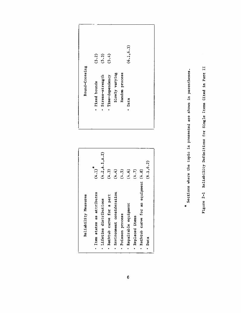
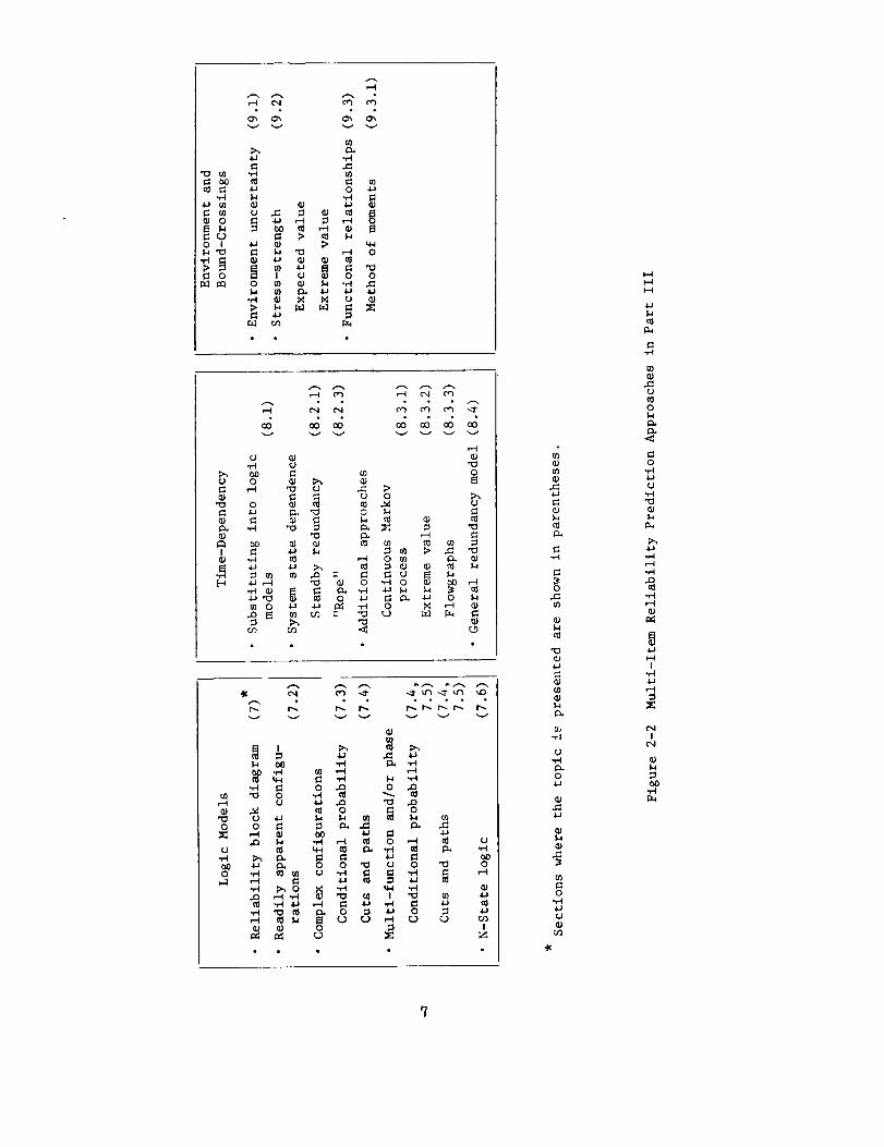
2.1 Prediction TechniquesFigure 2-1 showskey wordsassociatedwith reliability measuresof single items
and Fig. 2-2 does the samefor the conventional and classical reliability predictionmodelingapproachesfor multi-item systems. Thesections of this report wherethetopic is coveredare cited on the figures. Broadly speaking, the single item measuresof Fig. 2-1 can apply to various levels of systemaggregation, e.g., parts,equipment,andsystemlevels as well as to humanevents. That is, they offer indices
by which to describe someof the inputs to a multi-item reliability prediction andby which to express someof the outputs.
Reliability predictions implementedwith the approachesof Figs. 2-1 and 2-2have typical assumptionsand characteristics. Quite often these are unstated; theyare Just implied. Sometypical assumptionsand characteristics are:
(I) A "fuzzy" definition of the failure of items and system, is it: Out ofspecification? Simply inoperative? Completecatastrophic failure?
(2) Theprediction usually considers eachitem involved to have two states,either goodor bad. In most predictions this is reasonable; however,there are certain situations wherethis can lead to grossly incorrectresults. A familiar exampleis ignoring the two failed states of openor short of diodes in redundantarrangements.
(3) Independenceamongitems is liberally assumed. Included here is theimpact of not considering uncertainty in the natural or inducedenviron-ments.
(4) Prediction is for a mature product. A prediction is quite often muteon the assumptionthat most design andmanufacturing"goofs" havebeenremovedand that the necessaryburn-in period has beenpassed. This hasserious implications for items suchas those intended for spacewhichare producedin small quantity.
(5) Omissionof the humanelementduring operation.(6) Uncertainty in the parametersof single items are often not considered
explicitly. Techniquesof sensitivity analysis and of probabilistictreatment of uncertainty are potentially applicable.
5
n3
_D
Cxl o3 ...I- ,-4
u3 u3 u3 _Dv v v v
00
-H
m 3:: ;_h m
l_ 0o _ _ tJtj m _ _ 14 0
I "0 _ Pc; m W
0 33 I 0_ 0
"0 m I 0 r!.
14
m
_u
"i-I
-H,-4QJ_d
v v v v v v v v v
_ .,4W .u 0•6_ I_ -i-I o _
_ o _ _ om I_ 0 _o _ m
"_ o o. _
_ _ _J
• • • ) • • • • •
(I/
t_
-M
0
m
Wo_
'13
.l.l
_Jm
t8,i.-I
¢J,14
0
0
.l-I
m
0
o
m
)-,i
r_
_-4
04-4
m
,,-I4-IqJ
'I-I,--I
,.m-I
,-4I
Q_W
-r.Ir._
6
v v '_ v
u):>-,•IJ .1-I
_ _ 0
0 I=; ,u ,-_ :_ ,-_ 0
0 I _ _ :> u_"0 _ _ _ _ 0
_ 0 m (1} _ .H _C
•.,-I (_ X X 0
v v v
0
0C
0
[..-i
0C
v v v v
,,_0
:>0 :>_
0 _
_r--I "_ _.1 0 .MO O_ _ ,.-._•r-.I _
v v v v v v v
,,,M
o_0
u_ CC o
,__ _ o
0 0 _ _ C..C
,_ _ _., 0 0 _:1 0 0 _ 0
o., ,_, o _ g _ = _ _
• . • •
m
m
._d
m
r/)(11
C_
m°M
o
.x=.1_1
(1)
m
o
.iJ
C-H
_C
0
C.
0
,-4
I
w,-t
|
,.,.-I

Of course, exceptions in particular predictions will exist for these typical assump-
tions and characteristics. These apply to the majority, not the exceptional case.
2.2 Prediction Technique Choice
The approach used for a particular prediction is influenced by a myriad of
factors. Implications of some factors such as the commodity and its intended opera-
tional profile tend to be somewhat apparent. Here the need is mainly that of knowledge
about the various reliability prediction indices and equations of the sort noted
in Figs. 2-1 and 2-2. Other factors such as schedule and the extent of the intended
reliability program are more subjective in their implications. Here the influence
is more on the choice of parameter values rather than the choice of equations.
There is little which can be said on applying this technique to this situation
and that technique to that situation which is not apparent to someone who understands
what you are talking about. About all that seems appropriate is a plea to use common
sense, e.g., use the simplest approach commensurate with the purpose of the analysis
and the accuracy of the parameter data.
Life Cycle. Reliability prediction plays its major role during the planning
and early design phases of a program's life cycle. In these earlier phases of the
program a priori techniques of the sort described in this report are used. It can
be expected that there will be many iterations of a prediction as the program pro-
gresses, and that the prediction model will become more complex. When the program
progresses to the point that test and operational data start to become available,
then the a priori prediction techniques start to give way to the a posteriori tech-
niques of statistical inference. The reliability prediction model still has a role.
It provides a means for combining statistical inference estimates on items into a
composite measure for multi-item levels.
Con_nodity Considerations. Reliability prediction at the nonrepairable part
level is largely a matter of selection of the appropriate form from Part II by which
to express the reliability measure. This includes the designation of the stresses
which are appropriate. At the equipment level, say in the order of hundreds of piece
parts, the main consideration as to what technique is used depends largely on whether
the equipment is electrical or non-electrical. Electronic equipment typically uses
a very straightforward approach. The parts are assumed to have a constant failure
rate and failure rates are added to obtain the failure rate (or its reciprocal mean-
time-between failure) for the equipment (See Sec. 8.1.1). This approach is also
sometimes used for nonelectrical commodities, but often more involved prediction
techniques will be applied to mechanical or structural commodities. The stress-
strength approaches of Secs. 5.3 and 9.2 are structurally oriented, but they are
8

really specialized applications of broadly applicable approaches concerning environ-
ment effects which are noted in Secs. 4.4 and 9.1. At the system level the techniques
which are used tend to be quite varied and the entire scope of Part III is applicable.
Mission Implications. The operational time periods and the environments of
the operational profile, of course, affects the choice of the reliability prediction
technique. Space systems have been thus far of a one-shot nature with the main periods
of launch, orbit, and recovery. Launch and recovery environments tend to be somewhat
severe, whereas orbital environments tend to be moderate. A major constraint handicapping
reliability measurement prior to use has been the combined effects of the lack of
experience, the cost, and the small quantity of some commodity types. The decade
of space experience has alleviated these conditions to some extent. However, presently
the nature of space missions is being extended to deep space missions and eventually
to commodities reusable after recovery. Thus an increasing number of one-shot, non-
reusable commodities are on the verge of giving way to multiple use, repairable com-
modities. Space reliability predictions will thus start to take on more of a similarity
to predictions for systems intended for airborne and surface missions. These latter
types are as much concerned with the implications of repair, that is maintainability,
as they are with reliability. The typical airborne system which is not operating
continuously is desired to have a very high overall availability followed by a very
high reliability for relatively short missions. The overall availability here is
of a continuous nature and the missions are of a cyclic nature. Systems for surface
missions often are continuously operational, but they can quite often be removed
from operation for repair or maintenance. However, they usually will have short
periods of intense operation where no repair is possible. These short periods may
be somewhat predictable, as for space-oriented services, or they may be nonpredictable
as for military uses. Presentations on maintainability and availability prediction
techniques are available in Refs. 2 and 3.
Subjective Factors. The ultimate accuracy is primarily affected by the subjective
Judgment of the person performing the reliability prediction. Main considerations
are the kind of reliability program with attendant influences of budget, schedule,
and the operational environment. Historical experience in reliability prediction,
particularly where it has been followed up with reliability measurements, have helped
considerably in this area. Detailed listings have been made of the many variables
which are pertinent [Ref. 4] but in the final analysis this is largely a matter of
mental assimilation on the part of the person performing the prediction.
2.3 Related Analyses
Other types of analyses overlap and interface with reliability predictions.
Brief commentsare given belowon these allied studies. The comments are aimed pri-
marily toward the equipment and system level of commodity complexity, and particularly
toward the latter. System effectiveness is currently a popular phrase which is used
to cover the scope of the considerations cited below. Some system effectiveness
models have been proposed which attempt to pull together the appropriate ingredients
[Refs. 5 and 6]. This is possible to some extent with the gross models and their
attendant assumptions. A system effectiveness analysis will typically reflect the
effort of various individuals as it is unlikely that any one individual can master
or have the time to perform all of the analysis areas intended in any one program.
Other Reliability Analyses. During the planning and early design program phases
the other reliability analyses, in addition to prediction, can be classified into
failure mode and effects, performance variation, and stress as suggested in Ref. 7.
Failure mode and effects analyses are often probing to a level of detail which is
not reflected in the reliability prediction model. It is often of a seml-qualitative
nature. It is conceptually possible to reflect extremely detailed failure modes
into reliability prediction.* However, there are usually the practical reasons of
the unavailability of data and the complexity of such models which prevent a literal
one-to-one correspondence between the failure mode and effects analysis and a reliability
prediction.
The performance variation analysis is concerned with the area of reliability
prediction which in this report is referred to as bound-crossing. The reliability
discipline has promoted approaches for drift failure analysis of electronic circuits
which are commonly referred to as worst-case or as tolerance analysis techniques.
These have proved to be of value for purposes of reliability improvement. However,
they almost invariably are not extrapolated over into the reliability prediction
analysis. Again this is conceptually possible but usually not done for sound reasons.*
It should be noted that with mechanical and structural commodities there has been
greater use made of bound-crossing techniques for reliability prediction purposes.
A prominent example here would be the classical stress-strength model. Those which
are conventional or classical are noted in Parts II and III of this report.
Stress analysis typically has the most explicit relationship with a reliability
prediction.* This is because many of the reliability prediction manuals include the
applicable stress deratlng and failure rate adjustment tables and curves. Examples
are the effect of temperature, current or wattage levels on the failure rate. In
the nonelectronlc commodity the stress-strength model would be an example of a technique
which is common to stress and prediction analysis.
* Part IV of this report presents some thoughts on structuring a detailed reliabilityprediction model which explicitly incorporates this detail.
I0

Conventional Desisn Analyses. These traditionally involve both performance and
stress calculations and are what the design engineer would do to some extent regard-
less of whether he is explicitly concerned with reliability analysis. The performance
analysis is mainly related to the bound-crossing type of reliability measure and to the
performance variation analysis. The traditional deterministic, engineering equations,
relating performance attributes to part characteristics and other variables, become
part of the performance variation analysis. Similarly, the traditional deterministic
stress equations are developed and used by the designers. Calculation of safety margins
to such factors as voltage, power and temperature is a familiar form of this type of
stress investigation.
Saf_y. Systems analyses for manned space missions have always been directed
toward both safety and reliability. In terms of the impact on the reliability predic-
tion model, it usually turns out that the same, or slightly modified, prediction approach
will serve the safety prediction needs as well as those of reliability. For safety
there will typically be a different criterion of failure and a different operational
profile than for reliability. Also note that in nonspace types of systems, safety
analyses are also being performed [Ref. 8].
Availability and Maintainability. When repair is possible during application,
then availability and maintainability cannot be avoided in the prediction. This adds
a measure of complexity to the prediction technique, as the reliability prediction
literally becomes absorbed by the availability prediction. Some comments have pre-
viously been made on these analyses in Sec. 2.2 under the heading of Mission Implications.
Spares. Reliability prediction techniques have been experiencing increased
applications in spares planning and optimization. These may seem to be inseparable;
nevertheless, reliability analysis and spares analysis have been traditionally performed
by separate groups. Furthermore there are reasons which from the spares viewpoint
cause items to have higher failure rates than from the operational viewpoint. Examples
here would be the effects of secondary failures and the replacement of incorrectly
diagnosed failures. It is also noted that optimum spares allocation and optimum
redundancy allocations can use identical approaches.
Cost Trade-off. If cost-rellability relationships are available for single items,
then for some forms of multi-item configurations the literal optimization techniques
can be applied in order to obtain optimum reliability values for items. Also, to some
limited extent this can be expanded to include simultaneous optimization of reliability
and spares or reliability and maintainability. The main limitations here are the
accuracy of the cost-reliabillty or cost-maintainability relationships and those of
optimization techniques. Note also that the optimum allocation techniques find
application for other penalties than cost, e.g., volume, weight, power, or perhaps
simultaneous treatment for several of these.
II

The basic reliability allocation problem which is amenable to analytical solutiom
is that of selecting an optimum system configuration from allowable alternate design
approaches so that reliability is maximized subject to a penalty constraint, or vice-
versa. It is necessary to have a reliability prediction equation which covers the
range of allowable alternate design approaches and similarly a penalty prediction
equation. Thus one use of the suitable reliability prediction equations of this
report is to provide an input for a reliability allocation. An approach to this
problem can be developed based on the dynamic programming principle. As would be
expected exact solutions can be obtained from problems Which are usually too simple
to be of practical value. For example, Ref. 9 gives a dynamic programming procedure
for selecting exactly the order of the active redundancy in the case of one constraint
and of the active form of redundancy. Procedures for more realistic problems can be
developed but they usually yield an approximate solution. However, the incompleteness
usually will not result in differences of practical importance.
Refs. i0 and ii describe computerized approaches which are suitable for realistic
problems. The approach in Ref. i0 is for identifying an optimum redundancy configura-
tion where each item in the system can be active, standby with switch, or spare
redundancy. It is assumed that only one item must work, that the items have an
exponential failure distribution, and that the failure (or success) events for the items
are mutually independent. Ref. ii treats essentially the same problem ignoring the
switch but introducing the non-serial, e.g., a "bridge," configuration. The former
paper is patterned after the results in Ref. i0 but allows for more practical
redundancy alternatives.
It was decided that the result given in Ref. i0 could be generalized to include
the case in which at least n o items must work out of n items (n o < n). In order to
do this it was necessary to derive a general reliability prediction formula for
parallel arrangements, as shown in Sec. 8.4. This formula has been computerized and
the program is discussed in Volume II - Computation. This program is actually a sub-
routine in the general Reliability Cost Trade-off Program (RECTA). The subroutine
enables one to consider majority voting redundancy as well as the three types of
redundant items as noted above. Practical procedures for obtaining an optimum selec-
tion of the reliability of items in series can also be based on a dynamic programming
procedure. This is where reliability improvement of an item is improved by such means
as design and manufacturing emphasis on reliability and redundancy is not allowed.
The largest difficulty here is obtaining an accurate relationship between item relia-
bility and cost. The general reliability cost trade-off program (RECTA) cited above
simultaneously treats configurations containing series and the various redundancy
approaches. Here the allowable alternative for an item includes increasing the
12

reliability of the non-redundant item and/or making the item redundant. Any of these
alternatives can be disallowed, thus a generalized serles-parallel reliability alloca-
tion procedure.
RECTA as cited above was developed as part of an evaluation of computer
programs for system effectiveness [Ref. 12]. This reference and other sources will
call attention to the possible use of allocation procedures based on linear and
quadratic programming and on Lagrange multipliers. These approaches have usually not
proven suitable for realistic reliability-cost allocation problems.
IS

3. Needs and Problems
The largest need is that reliability prediction be included or be considered
as an essential element of the actual decision-making process. This is not Just
a matter of design engineers and managers tolerating the reliability prediction,
but rather one where the desired situation is that these persons need and want the
results of the prediction. The reliability prediction should be influencing the
design and operating plans, rather than a separate exercise whose outputs are ignored
or forced to Justify a preconceived design and operating plan. The problems here
are grouped into those concerning people, data, and techniques. These remarks are
not in the sense of criticizing anyone or any discipline; rather, they are intended
as unemotional commentary.
3.1 People
Reliability prediction utilizes heavily the mathematics of probability. Reli-
ability measurement and testing utilize the mathematics of statistical inference.
These are both complex subjects that are simply difficult to really learn. In addi-
tion to the practical knowledge required for applying them, the theory is also important.
The majority of technical persons, including designers, management, as well as reliability
engineers, typically have not had the opportunity to become well-versed in the mathematics
of probability and statistical inference prior to their initial attempts at using
them.
The solution here is not at all readily apparent. A probability or statistics
course or two in the college curriculum or a concentrated short course after college
really only helps the person co_unicate better with someone who is well-versed in
these subjects. Persons specifically trained in the mathematics of probability or
statistics, on the other hand, have their difficulties in understanding the engineering
applications. Such a person in a product-oriented organization will typically have
difficulty adjusting to the approximate nature of engineering mathematical models, to
the myriad of pertinent variables which cannot be reflected simultaneously in equations,
and to the situation that testing to satisfy statistical confidence often requires
unrealistically large sample sizes due to cost considerations.
There is some sentiment for having the design engineer also pick up the task
of reliability prediction and the other reliability analyses. There is much to be
said for this; after all, these persons, particularly at the equipment level, are
usually called upon to provide cost, weight, and other predictions in addition to
strict performance. It is generally accepted that the designer is "responsible"
for "designing reliability" into the equipment; it follows that he should have some
degree of responsibility for the reliability analysis of his design. For electronic
equipment this may be a reasonable approach. Some few suppliers are doing this.
14

They do not have reliability specialists, or if they do he performs the role of a
consultant. For structural and mechanical commodities and for systems, the reliability
prediction is more complex than for electronic equipment. The approach of having
the designer also perform the reliability prediction is more difficult here. Even
if management decides that the approach of having the designer perform the prediction
is desirable, it is still difficult to implement. These design people are already
generally overloaded in work schedules. Also, they may not be interested.
A nagging consideration to many persons is that the mathematics of probability
and statistics have enjoyed successful application in many areas, for example, communi-
cations, economics, biology, agriculture, and information theory. It seems that it
is the reliabillity area which perhaps uniquely has a somewhat unsuccessful history of
application of probability and statistics. At least the road here has been a lot
rougher than in other areas. One cannot help but feel that a major reason is that
many of the people who have been involved in reliability prediction - the people doing
them as well as other persons who are expected to use the results - have Just been
weak in the theory and practical applications of probability and statistics.
3.2 Data
Data refers to the actual numerical value of reliability indices for various
items. Thus data, one way or another, revert back to some type of reliability
measurement. Even once the need is recognized, there is the problem of how to go
about making reliability measurements. What is the best index? The greater the
reliability of any item, the more difficult it is to measure. Who is to pay for it?
A part or equipment supplier often will deliver his product and will never hear any-
thing further regarding reliability, particularly if it is satisfactory. Experience
with the reliability measurements of operational items have indicated that it is near
impossible to rely on operational and maintenance personnel to supply this data;
special persons have to go along Just to record the reliability information. In
addition, there is recognition of the situation that it is more glamorous to work
with models and equations than to try to record and interpret data.
Efforts, of course, have been made at gathering and disseminating data, and these
continue (Sec. 6 of this report contains some data references). These are to be
commended. Contractors are more and more developing their own data and making data
banks, but they are handicapped. More efforts are needed in the data area and of
necessity will require funding by various government agencies. Individual contractors
do not have wide access to operational sites, nor do they have much funding for this.
With regard to individual programs, there is a great opportunity for using sampling
techniques rather than to record everything, particularly with actual operating equip-
ment and systems, in order to gather needed information.
15

3.3 Techniques
A few co_ents are given here on the area of reliability prediction technique
needs; however, this is not as large a problem area as those of people and data. Con-
flicting positions can be easily taken. On one hand, it can be said that more complex
techniques are not generally going to be applied because invariably better data is
needed. It is unlikely that such data will become generally available. On the other
hand, it can be argued that complex situations require complex mathematical models.
In any case, efforts will continue for technique development. It is something that
can be done individually and without major funding. It is the sort of thing that
people who are inclined in this direction will continue to do whether they have a great
deal of support or not.
Computers seems to continue to get faster with larger storage. This opens the
door to more involved and more complex analyses. Rationale-wise, there is a need to
cycle more practical experience back into the development of prediction techniques.
This is now becoming possible more than previously because of the increased experience
with reliability prediction.
At the system reliability level, opportunity areas are more explicitly bringing
in the human impact and the environment, that is, treating the reliability of man as
well as the machine and treating other unknowns such as possibly the environment as
a probabilistic variable. At the equipment level a need is how to formulate proba-
bilistic models for treating distinct failure modes simultaneously with environment
(Part IV of this report presents some thoughts on this). At the systems level again,
there is a need for improved methods to tie together maintainability, spares, per-
formance, and cost with reliability. This has been labeled systems effectiveness, and
there are efforts under way here as noted in Sec. 2.2.
Also to be given due consideration is the opportunity for less complex methods,
that is, striving for balance between complexity of the prediction technique and
accuracy of the result. There are places for simple rules of thumb and for simple
estimating relationships.
16

Part II. Single Item Reliability
In this part the concept of reliability measures for a single item are discussed
from a broad viewpoint. The reliability measures consider two basic categories of
problems: (i) those in which an item is in either a success or in a failed state
(considered in Sec. 4) and (2) those in which certain characteristics of an item
may be of an unacceptable value, the "bound-crossing" problem (considered in Sec. 5).
Guidance on obtaining numerical index values for a single item of both categories is
given in Sec. 6.
These reliability measures are potentially applicable to any item or event to
be considered in a prediction. Thus inputs for multi-item prediction equations would
be of one of the forms covered, as would the output of the prediction. Or, if the
reliability measures for an item is obtained from testing, then inferences would be
made concerning these measures.
These definitions will, in the main, be well-known to reliability workers.
Some features are covered, however, which are not emphasized in existing handbooks
and books. These are the following: Possible confusion concerning mathematical
descriptions of the widely cited bathtub curve when it is used for non-repairable
items such as parts versus for repairable items such as equipment is discussed in
Secs. 4.3 and 4.8. Uncertainty in the environment is discussed in Sec. 4.4.
Explicitly bringing time into consideration for bound-crossing problems is introduced
in Sec. 5.4, where possible failure criteria for non-monotonic drift requires
careful treatment.
lq
4. Reliability Measures
Various indices used for reliability measures are described in this section,
and there is a probing beyond conventional assumptions. The material gets progres-
sively more involved, starting with simpler notions and models. The later part of
this section goes into considerations of reliability measures for repaired items.
4.1 Definitions of States and Reliability
The simplest way of classifying the state of an item is as two states,
success (S) and failure (F). Let P(S) be the probability of success and P(F) be the
probability of failure of the item subject to given conditions under which the
probability measures are to be defined.
R = P(S)
1 - R = P(F)
P(S) + P(F)
Then
= probability of success,
= probability of failure, and clearly
= 1.
This simple classification and the associated indices of reliability and unreliability
are based on several assumptions such as the following:
(i) a definition of failure exists,
(2) the probabilities of success (or failure) are conditional on a known
(deterministic environment, or on known characteristics of environment
described by probabilistic measures, and
(3) the classification is for a certain future time instant or time interval.
Much of the subsequent material in this section involves expanded treatment of these
assumptions. The assumptions should be kept in mind, but more important, they should
also be kept in perspective. Most definitions and mathematical models are based on
assumptions which are not fully met when associated with real world situations. The
delicate question is always one of the effects of violation or relaxation of the
assumptions for the problem which is at hand. Sometimes extremely simple equations
will do the Job; at other times extremely complex equations are needed. In some
situations the state of an item should be subdivided into three states S, FI, and F 2
for an adequate approximation to real world application. F 1 and F 2 are two different
failure modes and the probability identity can be written as
P(S) + P(F I) + P(F 2) = 1.
Some examples for consideration of two failure modes are digital circuits, relays,
switches, and diodes. In general, any reasonable number of states may be associated
with the various modes which an . item might assume. Some additional comments concerning
mathematical descriptions of multiple failure modes appear in Sec. 4.3.
18
It is desired to broaden one's concept of failure to include the many possible
types which may occur. Some examples of failure modes are given below.
(i) The performance of an item deviates from its nominal value by more
than i0 percent.
(2) A diode opens or shorts.
(3) An amplifier is "noisy".
(4) An accumulation of the effects of a somewhat periodic variation of the
performance of an item outside given bounds. _
(5) Corrosion of a boiler tube.
(6) Fracture of a pressure vessel.
These various types of failure are introduced to motivate one to pay attention to
possible ways in which items can fail and hence not overlook any important details.
4.2 Reliability as Function of Time
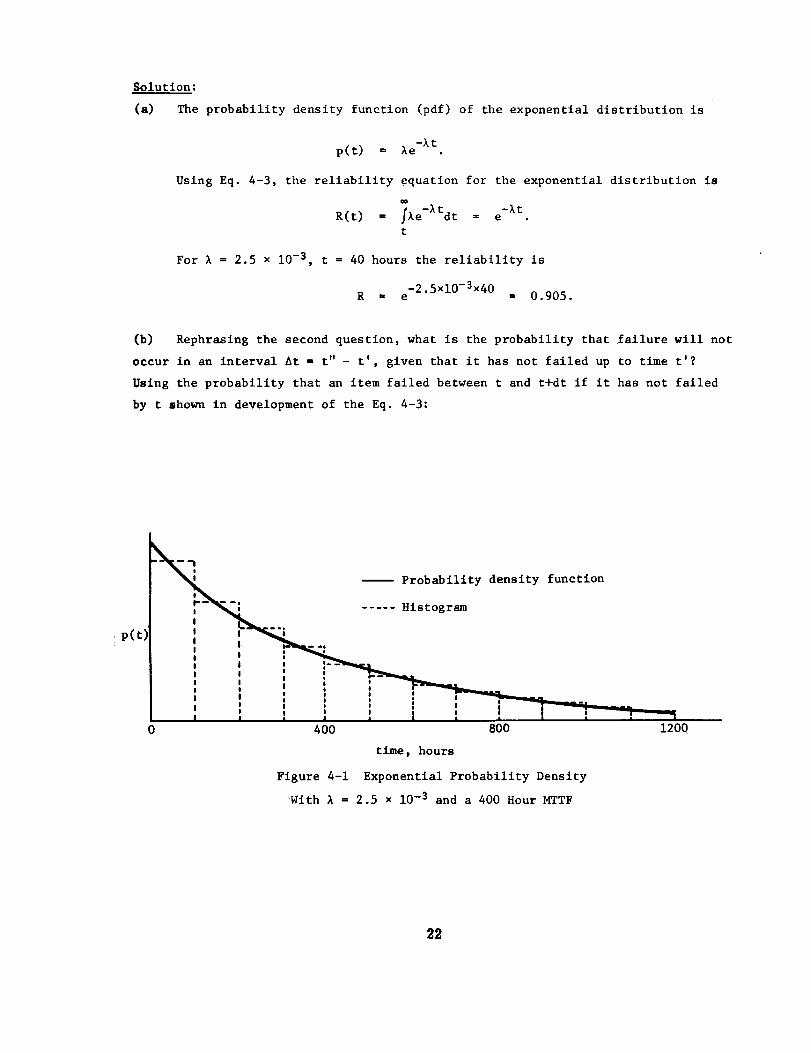
The probability density function of time to failure of an item will be used as
the starting point, as this can be visualized easily from a histogram of time to
failure data. In Fig. 4-i a histogram is shown as dashed and the associated
probability density is the continuous function.
(i) The probability density of failure as a function of time t is
p(t), t > O. (4-1)
(2) The probability of failure of the item by time t is the cumulative
probability t
F(t) = fp(t)dt. (4-2)0
(3) Reliability is the probability of no failure by time t
R(t) = 1 - F(t) = 7p(t)dt. (4-3)
t
(4) The hazard rate is the conditional probability of failure given
that the item has not failed by time t. Other terms widely
used for hazard rate are failure rate (when exponential failure
density function applies), instantaneous failure rate, or force
of mortality.
The probability relationship concerning two dependent events can be used to develop
the hazard rate. Recall that*
p(AIB) P(_)= P(B)
Basic probability definitions and relationships are presented in Appendix A.4.
19
If: P(AIB)
Hence
P(AB)
P(B)
= h(t)dt = probability that an item fails between t and t+dt, given
that it has not failed by t,
= p(t)dt = probability that an item has not failed by t and that it
fails between t and t+dt, and
= R(t) = probability that an item has not failed by t.
P(A[B) = P(_) = p(t)dtP(B) R(t) '
h(t)dt = p(t)dt or h(t) = p(t) (4-4)R(t) ' R(t) "
The hazard rate function h(t) can also be obtained using the fact that it is an
instantaneous failure rate.
h(t) = llm F(t+At) - F(t) i _ p(t)At_O At R(t) R(t)
It can also be expressed as follows:
-R'(t) _- _ din R(t)h(t) -
R(t) dt '
where R'(t) is dR/dt. Reliability can now be expressed as
R(t)
t
= exp{-fh (t)dt}.0
(5) The mean time to failure, MTTF, is the expected time to failure.
The expected value of a random continuous variable x is
E(x) = 7x p(x)dx
or in the above notation
° 7E(t) -- MTTF -- it p(t)dt -- R(t)dt (4-5)0 0
The last result can be seen by integrating by parts the following
_t R'(t)dt, R'(t) -dR
dt "0
The definitions in Eqs. 4-1 through 4-5 were developed for time as a
continuous variable. In some situations it is appropriate to measure time as a
discrete variable, where the number of cycles or operations to failure is a discrete
2O
variable. The definitions in Eqs. 4-1 through 4-5 have direct counterparts for handling
discrete variables. These counterparts for the discrete variable case are shown below,
where n is the number of cycles to failure [Ref. 13].
Probability density:
Probability of failure:
Reliability:
Hazard rate:
Mean cycles to failure:
p(n), n = i, 2, 3, ... (4-6)
n
F(n) = _ p(n) (4-7)
R(n+l) = i - F(n) (4-8)
p(n) (4-9)h(n) = R(n-l)
MCTF = _ n p(n). (4-10)i
A large number of possible probability density functions (discrete and
continuous forms) have been proposed. Several are shown in Appendices A.I and A.2.
Although these density functions are presented with reference to lifetimes, there are
also other possible applications of these same density functions in reliability
analysis. Some of these density functions will again appear in subsequent sections
of this volume. See Ref. 14 for some good examples of application of various
density functions for reliability purposes.
The exponential density function is widely used in reliability prediction and
its key feature, a constant hazard rate, is illustrated below in Ex. 4-1. One of
the most common misconceptions appearing in the reliability literature is the
implication that a random failure law and the exponential failure law are one and
the same. Assuming a random failure law simply implies that failure times occur
randomly over time according to the stated probability distribution, there can be
any number of distributions or laws depending upon whether the log-normal, the
Weibull, the gamma or some other distribution is assumed to best describe the
distribution of failure times.
Example 4-1
A high-power magnetron has an exponential distribution of time tofailure with a failure rate of 2.5 x 10 -3 failures per hour. The probabil-
ity density function of Fig. 4-1 is of this item. (a) What is the relia-
bility for a new magnetron for the first 40 hours of operation? (b) What
is the reliability for the following 40 hours of operation if the
magnetron has not failed during the first 40 hours?
21
Solution:
(a) The probability density function (pdf) of the exponential distribution is
-Xtp(t) = Xe
Using Eq. 4-3, the reliability equation for the exponential distribution is
-_tdt -XtR(t) = = et
For X = 2.5 x 10 -3 , t = 40 hours the reliability is
-2.5xlO-3x40R = e = 0.905.
(b) Rephrasing the second question, what is the probability that failure will not
occur in an interval At = t" - t', given that it has not failed up to time t'?
Using the probability that an item failed between t and t+dt if it has not failed
by t shown in development of the Eq. 4-3:
p(t)
-[_ -- Probability density function
I ,_
_; ..... Histogram
, i : ; , _m_m._..' ' ; I I ,'.,' '.,' i, ! i i ! | I ;• m I I I I I
0 400 800 1200
time, hours
Figure 4-i Exponential Probability Density
With _ = 2.5 × 10 -3 and a 400 Hour MTTF
22
t I!
fp (t)dtt'
R = 1R(t')
= 1 - R(t') - R(t") = R(t")R(t') R(t')
In the example problem for the exponential distribution
R -
-At" -%(t'+_t)e e
-At' -%t'e e
-_Ate
-2.5%10-3x40= e _ 0.905.
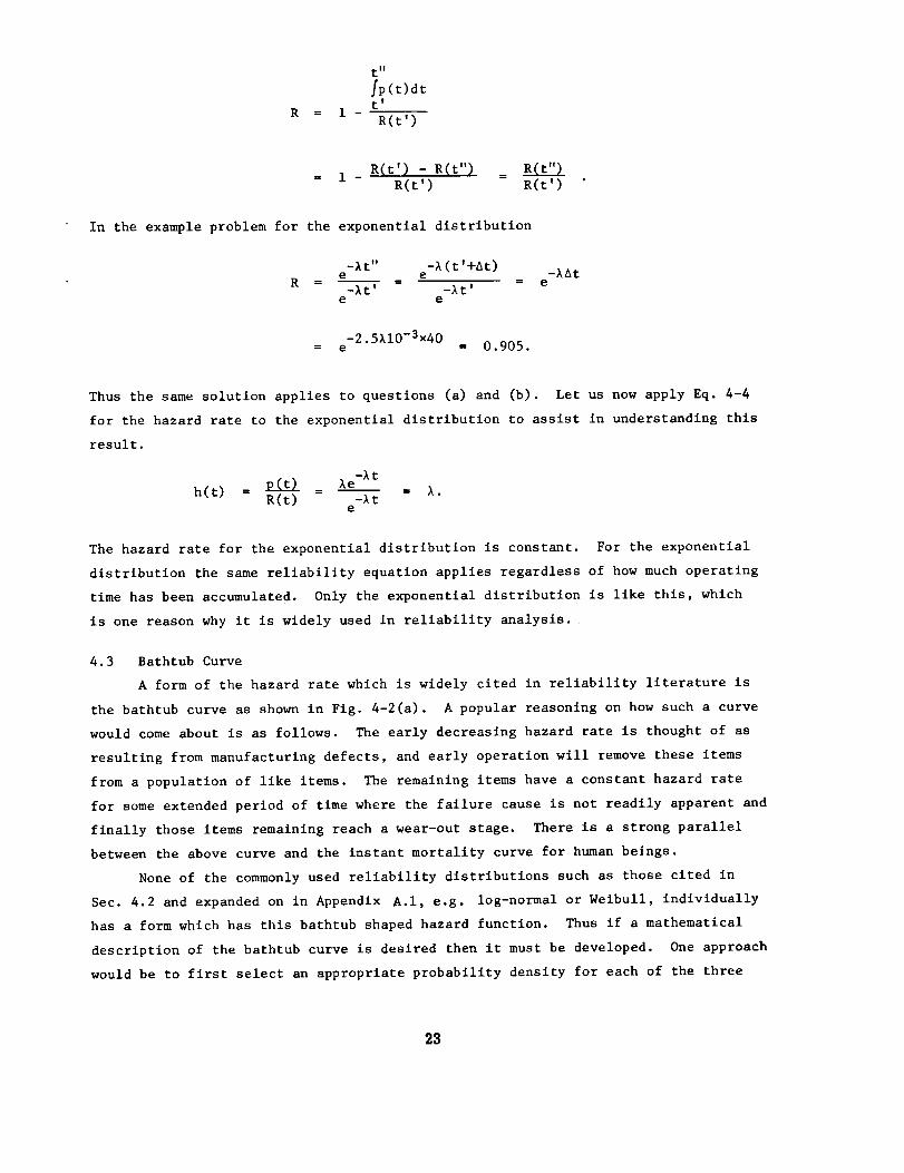
Thus the same solution applies to questions (a) and (b). Let us now apply Eq. 4-4
for the hazard rate to the exponential distribution to assist in understanding this
result.
p(t) %e -%t
h(t) = R(t) = -_t = _"e
The hazard rate for the exponential distribution is constant. For the exponential
distribution the same reliability equation applies regardless of how much operating
time has been accumulated. Only the exponential distribution is like this, which
is one reason why it is widely used in reliability analysis.
4.3 Bathtub Curve
A form of the hazard rate which is widely cited in reliability literature is
the bathtub curve as shown in Fig. 4-2(a). A popular reasoning on how such a curve
would come about is as follows. The early decreasing hazard rate is thought of as
resulting from manufacturing defects, and early operation will remove these items
from a population of like items. The remaining items have a constant hazard rate
for some extended period of time where the failure cause is not readily apparent and
finally those items remaining reach a wear-out stage. There is a strong parallel
between the above curve and the instant mortality curve for human beings.
None of the commonly used reliability distributions such as those cited in
Sec. 4.2 and expanded on in Appendix A.I, e.g. log-normal or Weibull, individually
has a form which has this bathtub shaped hazard function. Thus if a mathematical
description of the bathtub curve is desired then it must be developed. One approach
would be to first select an appropriate probability density for each of the three
23
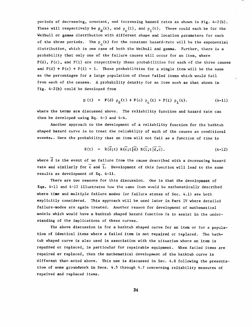
periods of decreasing, constant, and increasing hazard rates as shown in Fig. 4-2(b).
These will respectively be Pd(t), and Pc(t), and Pi(t). These could each be for the
Weibull or gamma distribution with different shape and location parameters for each
of the three periods. The Pc(t) for the constant hazard-rate will be the exponential
distribution, which is one case of both the Weibull and gamma. Further, there is a
probability that only one of the failure causes will occur for an item, where
P(d), P(c), and P(i) are respectively these probabilities for each of the three causes
and P(d) + P(c) + P(i) = i. These probabilities for a single item will be the same
as the percentages for a large population of these failed items which would fail
from each of the causes. A probability density for an item such as that shown in
Fig. 4-2(b) could be developed from
p (t) = P(d) Pd(t_ + P(c) Pc(t) + P(i) Pi(t). (4-11)
where the terms are discussed above. The reliability function and hazard rate can
then be developed using Eq. 4-3 and 4-4.
Another approach to the development of a reliability function for the bathtub
shaped hazard curve is to treat the reliability of each of the causes as conditional
even_s_. Here the probability that an item will not fail as a function of time is
R(t) = R(_;t) R(_;tld) R(T;tld,c ). (4-12)
where d is the event of no failure from the cause described with a decreasing hazard
rate and similarly for c and i. Development of this function will lead to the same
results as development of Eq. 4-11.
There are two reasons for this discussion. One is that the development of
Eqs. 4-11 and 4-12 illustrates how the same item would be mathematically described
where time and multiple failure modes (or failure states of Sec. 4.1) are both
explicitly considered. This approach will be used later in Part IV where detailed
failure-modes are again treated. Another reason for development of mathematical
models which would have a bathtub shaped hazard function is to assist in the under-
standing of the implications of these curves.
The above discussion is for a bathtub shaped curve for an item or for a popula-
tion of identical items where a failed item is not repaired or replaced. The bath-
tub shaped curve is also used in association with the situation where an item is
repa_ed or replaced, in particular for repairable equipment. When failed items are
repaired er replaced, then the mathematical development of the bathtub curve is
different than noted above. This use is discussed in Sec. 4.8 following the presenta-
tion of some groundwork in Secs. 4.5 through 4.7 concerning reliability measures of
repaired and replaced items.
24
(a)
Hazard-rate,
h(t)
Decreas-
ing
hazard
or burn-
in
Ii
Constant
Hazard
Time, t
Increasing
hazard or
wear-out
(b)
Probability
density
p(t)
Time, t
Figure 4-2 The Bathtub Shaped Hazard-Rate Curve
and Its Probability Density
25
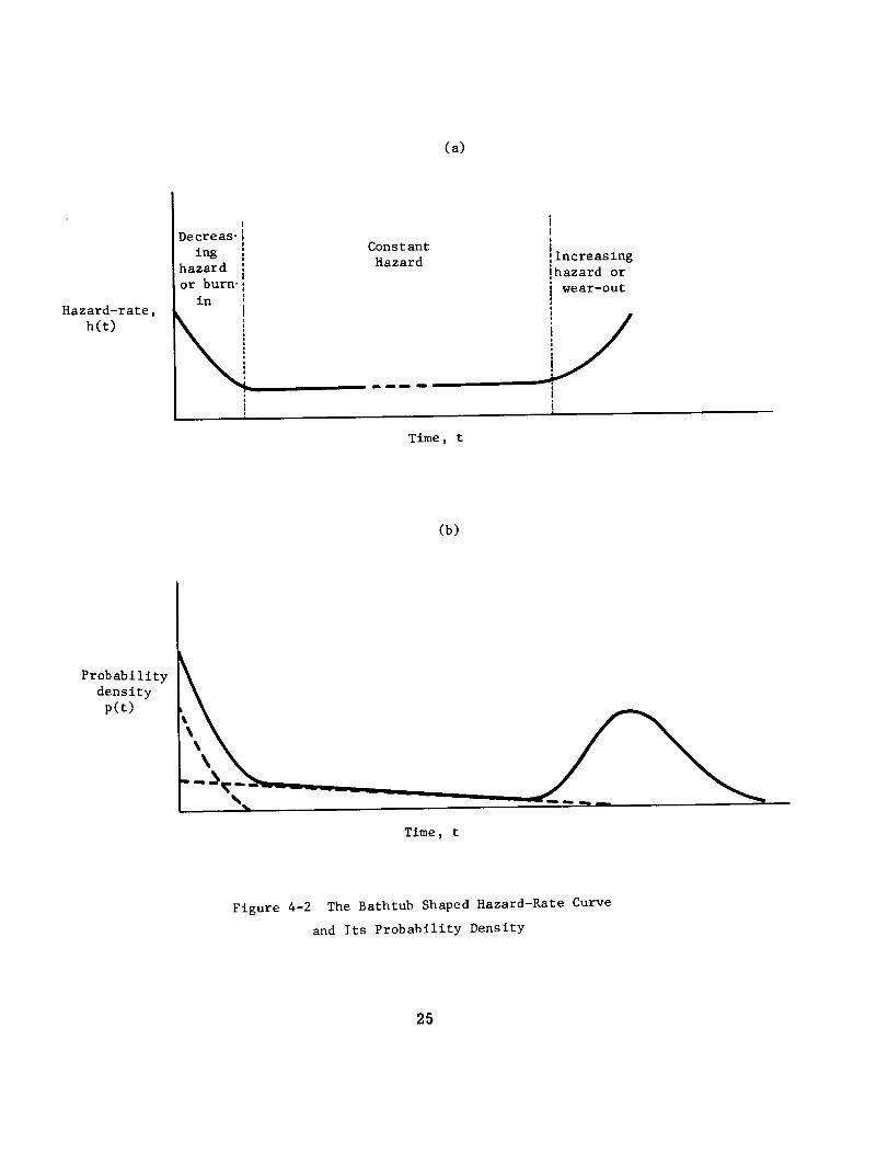
4.4 Consideration of the Environment
The reliability of an item is defined as the probability that an item performs
its intended function under defined conditions at a designated time for a specified
operating period. Thus the reilabillty is conditional on a specific environment or
environmental profile whether it is estimated by a simulated test or from results of
items used in previous missions. The environment might be characterized by fixed
conditions, such as temperature equal to 30°C, or it may be described by a deterministic
profile, such as that shown in Fig. 4-3.
T
E-4
Time
Figure 4-3 Example of Deterministic Environmental Profile
The environment might also be characterized by a random variable or a random
process where time is explicitly considered. Some approaches to considering the
effect of random environments on reliability measures are discussed below.
If the environmental stress is described by its density function p(E), then
the probability of successful operation is given by the following procedure. Let
the conditional probability of success given E be denoted by
P(SlE),
then the unconditional probability of success for continuous density function, p(E),
is given by
P(S) = fP(SIE) p (E) dE (4-14)E
26
and for discrete density function, P(Ei) , i = i, 2, ..., by
P(S) = I [P(SIEi) P(Ei) ].i
(4-15)
Example 4-2
Consider the simple example in which the probability density
for the environment is discrete as given below.
1
for E1
1P(E i) = _ for E2,
ifor E 3
and let the probability of success conditional on these environments be
p(SiEl ) = 48
P(SIE2) = 8
p(SIE3 ) = !8 "
Then the unconditional probability of failure is
[I'P(S'Ei) P(Ei)] 1 4 i 3 i I iiE
i
The above concept also cmn be used when an event requires an elapsed time period
(such as S = no failure to time t) and also when the environments are time
dependent.
In some situations it is necessary to explicitly consider the environment
a random process with known characteristics. Consider the problem where an item
will sometimes fail when an environment which is a random process reaches a certain
level. If the environment is a random process with peaks the distance between which
is given by the negative exponential distribution (assuming they occur with rate A
per unit time period) and if the conditional probability of failure is p given that
a peak has occurred, the probability that the item does not fail in the interval
(0, t) is given by
27
P(S) = P(no peaks in (0, t)) + P(1 peak in (0, t))q
+ P(2 peaks in (0, t)) q2 + ...
-%t -_t
-At (_t) e (At) e q2 += e + i! q + 2! "'"
-Apt= e
Thus the failure time distribution is exponential under this environment. See
Refs. 15 and 16 for further discussion on this and related descriptions of a random
environment. Further, if an item will fail only after k peaks or shocks have occurred,
the gamma density function is appropriate. That is
%k tk-I e-%t
Pk (t) = r(k) ' t _> 0
where
Pk(t) = 0, elsewhere, (4-16)
t is time,
is the rate at which the shocks occur,
k is the number of shocks for failure, and
r(k) = (k-l) ! = (k-l) (k-2) "'" i.
In summary, the nature of the environment must be considered carefully to
hypothesize models for behavior of the reliability function.
4.5 Poisson Processes
The Poisson process is widely assumed in reliability prediction, particularly
for repairable items such as the typical electronic equipment.
Let Pn(t) = probability that exactly n occurrences are recorded during a
time interval of length t.
Thus Po(t) -- probability of no occurrences, and
1 - P0(t) -- the probability of one or more occurrences.
It is assumed that
l-Po (t)lim -_ A, that is the probability of one
tt+O
or more occurrences is proportional to the length of the interval, _ is a positive
constant, the failure rate of an item. See Ref. 17 for a detailed development of
this process and related birth and death processes.
28
Postulates: Whatever the number of occurrences in the interval (0, t), the following
conditional probabilities hold
P(an occurrence in the interval (t, t+h))
P(more than one occurrence in (t, t+h)) =
-- Ah+o (h) ,
o(h).
The above postulates yield the following difference equations.
P (t+h) = P (t)(l-Ah) + Pn_l(t)Ah + 0(h), n > 1 (4-17)n n
i.e., the probability that there are n occurrences in the interval (0,t+h) is the
probability of n occurrences in the interval (O,t) multiplied by the probability
of no occurrences in the interval (t,t+h), plus the probability of n-i occurrences
in the interval (0,t) and one occurrence in the interval (t,t+h), plus the probability
of n-x (x _ 2) occurrences in (O,t) and x(_ 2) in the interval (t,t+h), (the latter
is of order o(h)). For n = 0
P0 (t+h) = P0(t) (l-Ah)or
P0(t+h) - P0(t)
= -APo(t )h
and as h + 0 one obtains
dP 0 (t)
dt = -AP0(t) or P_(t) = -AP0(t).
Using P0(0) = 1 we get P0(t)
the differential equation
-At= e Equation 4-17 similarly can be reduced to
P'(t) = -AP (t) + AP n l(t) n > i. (4-18)n n - ' --
Substituting into Eq. 4-18, we obtain
Pl(t) = Ate -At '
We derive successively all the terms to obtain the general terms
-At n
P (t) = e (At)n nl , n = 0, i, 2 ..... _. (4-19)
lira :* o(h) is a function of h such that h__O__--_-- j O.
99
This formula gives the probability that n occurrences will be observed in a time
interval (0,t) with a constant rate of occurrence per unit time equal to A. The
quantity At is the expected number of occurrences in the time interval of length t
and one frequently sees the form
-_ n
P (t) e 9___n - n! ' (4-20)
where _ is the expected number of occurrences in the time interval of length t.
Example 4-3
Suppose that an item has a failure rate, A, of 0.001/hour. What
is the probability that no failures occur in i00 hours?
Solution:
Thus
At = i00 (.001) : 0.i.
-At -0.iP(0 failures) = e = e
Note that this is equivalent to the reliability of the item. Hence one can better
understand the tle-ln between the Poisson distribution and the exponential distribution.
Example 4-4
Suppose that a certain item is tested as follows. One item is
placed on test until failure and it is then replaced by another identical
item, etc. Suppose further that the failure rate of the item is 0.001/
hour and that the test is for i0,000 hours. What is the probability of
at least 15 failures?
Solution:
At is equal to 0.001 (10 %) = 10, the expected number of failures in 10 _ hours.
Thus the probability of at least 15 failures is given by
e-At (lt)n -i0: _ = _ e i0 n
P(n > 15) n 15 n! n 15 n!- 0.083
using Molina's Tables [Ref. 18 ] for the Poisson distribution. The same solution
would apply to the above problem if a single item was repaired and returned to
operation. Here the operating times between failure would be exponentially dis-
tributed, and the equipment reliability index, Mean Time Between Failure (MTBF), is
the mean of this distribution. Only the operating time would be considered. Further,
the same solution would apply to any number of identical items operated for a total
time of I0,000 hours, regardless of how much time was accumulated on any item.
3O

A reason why the Poisson process is widely assumed in reliability prediction
is that in this mathematical model past operation has no influence on future relia-
bility. This simplifies a prediction analysis; for some complex systems it makes
the prediction practical.
4.6 Reliability Measures for Repaired Items
Reliability descriptions for repairable items are discussed here for a
general situation where an example of such an item would be a motor or typical
electronic equipment. With repair, there are time (of operation) to first failure,
time between first and second failure, time between second and third failure, and
so on. Each of these failure times when considered for a large number of identical
items will have a distribution associated with it; these distributions may or may not
be identical.
The data from motor failures [Ref. 19] have indicated time between failure
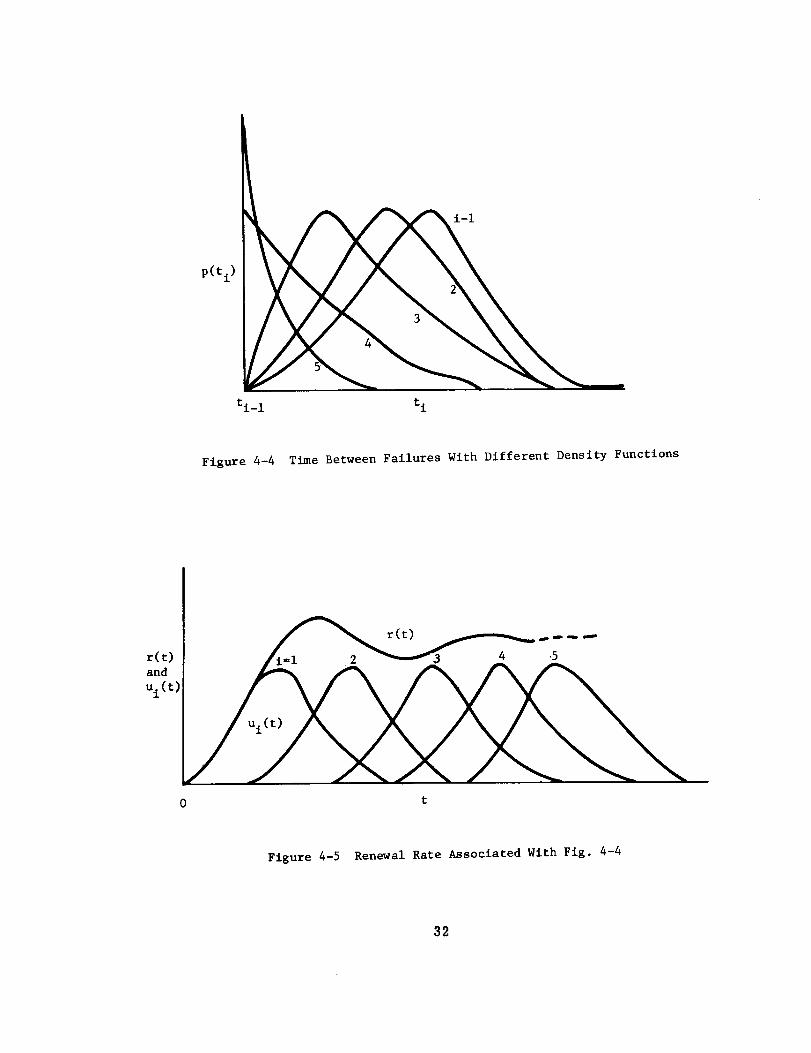
patterns as in Fig. 4-4. Density functions of the time to first failure, time
between first and second failure, time between second and third failure, and so on
are shown in Fig. 4-4, and these could be fitted with Weibull distributions with
different shape and scale parameters. The origin of each density function is when
operation is resumed after the motor is repaired. When the density functions are
plotted on an elapsed operating time scale, starting with the earliest initial
operation, then only the time to first failure density function is as shown in
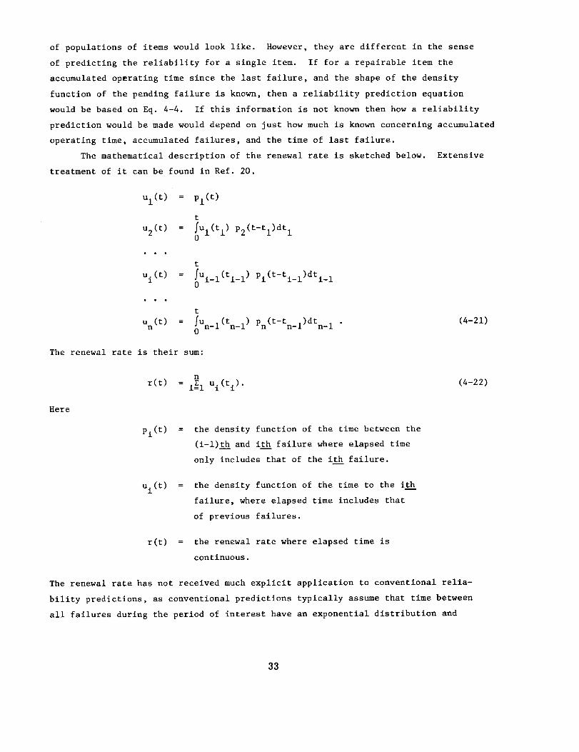
Fig. 4-4 and the others have a different shape. This is illustrated in Fig. 4-5.
The density function of the time to second failure on the scale in Fig. 4-5 is the
sum of the time to first and time between first and second failure; the time to
third failure is the sum of the first, second and third, and so on. There is
considerable overlap on the time scale of Fig. 4-5; as an example the early overlap
of the first and second times comes about because some of the first failures occur
late, which are repaired, and the second failure occurs shortly. The overlap
reflects the many possible combinations by which the first and second failures can
occur. As the third, fourth, and additional failures are brought into consideration,
they enter into the overlap on the elapsed operating time scale in a similar manner.
The summing operation is referred to as convolution. Fig. 4-5 also illustrates the
renewal rate, which represents the total number of items failing per unit of time,
divided by the original population. It can be seen to be the sums of the ordinates
of all the density functions of the time to failure as a continuous function of time.
Note that this is a conventional deterministic, algebraic summing, and is thus dif-
ferent from the probabilistic convolution type summing noted above. The renewal
rate where an item is repaired is similar in one sense to the density function of the
non-repairable item, as their shapes are what the smoothed curves for histograms
31
P(t i)
ti_ I ti
Figure 4-4 Time Between Failures With Different Density Functions
r(t) l l_-i 2 __ J 5and
ui(t)
0 t
Figure 4-5 Renewal Rate Associated With Fig. 4-4
39
of populations of items would look like. However, they are different in the sense
of predicting the reliability for a single item. If for a repairable item the
accumulated operating time since the last failure, and the shape of the density
function of the pending failure is known, then a reliability prediction equation
would be based on Eq. 4-4. If this information is not known then how a reliability
prediction would be made would depend on just how much is known concerning accumulated
operating time, accumulated failures, and the time of last failure.
The mathematical description of the renewal rate is sketched below. Extensive
treatment of it can be found in Ref. 20.
ul(t ) = Pl(t)
t
Ue(t) = ful(t I) P2(t-tl)dt I0
t
u.(t) = lu. _(t..) Pi(t-ti_l)dti_ 1i 0 z-± z-±
t
u (t) = fUn_l(tn_ l) Pn(t-tn_l)dtn_ l •n 0
The renewal rate is their sum:
(4-21)
Here
r(t)
Pi (t)
u.(t)1
r(t)
n
: iZ1 ui(ti)"
= the density function of the time between the
(i-l)th and it h failure where elapsed time
only includes that of the it h failure.
= the density function of the time to the it h
failure, where elapsed time includes that
of previous failures.
= the renewal rate where elapsed time is
continuous.
(4-22)
The renewal rate has not received much explicit application to conventional relia-
bility predictions, as conventional predictions typically assume that time between
all failures during the period of interest have an exponential distribution and
33
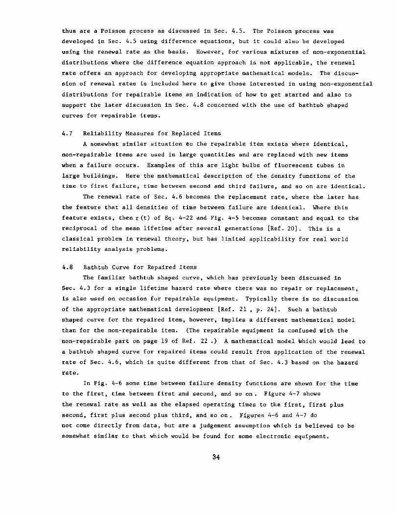
thus are a Polsson process as discussed in Sec. 4.5. The Poisson process was
developed in Sec. 4.5 using difference equations, but it could also be developed
using the renewal rate as the basis. However, for various mixtures of non-exponential
distributions where the difference equation approach is not applicable, the renewal
rate offers an approach for developing appropriate mathematical models. The discus-
sion of renewal rates is included here to give those interested in using non-expgnential
distributions for repairable items an indication of how to get started and also to
support the later discussion in Sec. 4.8 concerned with the use of bathtub shaped
curves for repairable items.
4.7 Reliability Measures for Replaced Items
A somewhat similar situation eo the repairable item exists where identical,
non-repairable items are used in large quantities and are replaced with new items
when a failure occurs. Examples of this are light bulbs of fluorescent tubes in
large buildings. Here the mathematical description of the density funntions of the
time to first failure, time between second add third failure, and so on are identical.
The renewal rate of Sec. 4.6 becomes the replacement rate, where the later has
the feature that all densities of time between failure are identical. Where this
feature exists, then r(t) of Eq. 4-22 and Fig. 4-5 becomes constant and equal to the
reciprocal of the mean lifetime after several generations [Ref. 20]. This is a
classical problem in renewal theory, but has limited applicability for real world
reliability analysis problems.
4.8 Bathtub Curve for Repaired Items
The familiar bathtub shaped curve, which has previously been discussed in
Sec. 4.3 for a single lifetime hazard rate where there was no repair or replacement,
is also used on occasion for repairable equipment. Typically there is no discussion
of the appropriate mathematical development [Ref. 21 , p. 24]. Such a bathtub
shaped curve for the repaired item, however, implies a different mathematical model
than for the non-repairable item. (The repairable equipment is confused with the
non-repairable part on page 19 of Ref. 22 .) A mathematical model _hich would lead to
a bathtub shaped curve for repaired items could result from application of the renewal
rate of Sec. 4.6, which is quite different from that of Sec. 4.3 based on the hazard
rate.
In Fig. 4-6 some time between failure density functions are shown for the time
to the first, time between first and second, and so on. Figure 4-7 shows
the renewal rate as well as the elapsed operating times to the first, first plus
second, first plus second plus third, and so on. Figures 4-6 and 4-7 do
not come directly from data, but are a judgement assumption which is believed to be
somewhat similar to that which would be found for some electronic equipment.
34
Each of the time between failure density functions of Fig. 4-6 is assumed to be
exponential in shape, but with some differences in the mean time to failure parameters.
The first two density functions have successively increasing means, the third density
function on through a very large number, n, have the same mean, and the n+ist and
successive density functions have decreasing means. Combining these time between
failure density functions into a renewal rate is illustrated in Fig. 4-6, which has
the familiar bathtub shape.
P(t i)
i P(ti)
1 a
2 b
3 through n c
n+l b
n+2 a
ti-i t i
Figure 4-6 Exponential Time Between Failure Densities with Different Means
35
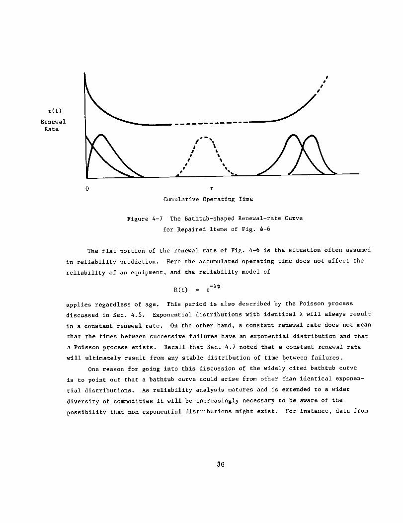
r(t)
Renewal
Rate
#
0 t
Cumulative Operating Time
Figure 4-7 The Bathtub-shaped Renewal-rate Curve
for Repaired Items of Fig. 4-6
The flat portion of the renewal rate of Fig. 4-6 is the situation often assumed
in reliability prediction. Here the accumulated operating time does not affect the
reliability of an equipment, and the reliability model of
-_R(t) = e
applies regardless of age. This period is also described by the Poisson process
discussed in Sec. 4.5. Exponential distributions with identical _ will alwmys result
in a constant renewal rate. On the other hand, a constant renewal rate does not mean
that the times between successive failures have an exponential distribution and that
a Poisson process exists. Recall that Sec. 4.7 noted that a constant renewal rate
will ultimately result from any stable distribution of time between failures.
One reason for going into this discussion of the widely cited bathtub curve
is to point out that a bathtub curve could arise from other than identical exponen-
tial distributions. As reliability analysis matures and is extended to a wider
diversity of commodities it will be increasingly necessary to be aware of the
possibility that non-exponential distributions might exist. For instance, data from
36

a population of repaired equipment when plotted in histcgram fashion might resemble
the bathtub curve, but the distribution of time between failures need not be
exponential. Correct choice of underlying distributions can have high implications
for the accuracy of reliability predictions, for the validity of statistical tests,
and for the optimization of preventive maintenance actions based on assumed
distributions.
37
5. Bound-Crossing
The type of reliability measures treated in this section are those sometimes
labeled tolerance, drift or degradation, better described as a "bound-crossing" type.
Items are designed to meet given requirements such as the output voltage of an
electronic power supply shall be 115 _ 1 volt ac and it is designated as failed if
the voltage crosses one of the bounds 114 and 116 volts ac. In a mechanical system
it may be desired to estimate the probability that the strength of an item will
exceed the stress to which it is subjected. In some environments the strength of an
item will be a function of time as a result of fatigue due to thermal cycling or
stress cycling. In this case we will be interested in the probability that at the
mission end the item will have sufficient strength to meet the applied stress. The
bound in this case is not necessarily a fixed level but may be a distribution of
stress levels.
5.1 Fundamentals
5.1.1 Notation
The notation to be used in this section will be y for a performance charac-
teristic, s for stress level or environment level, and t for time. The bound will be
denoted by £ for lower and u for upper.
5.1.2 Bound-Crossing Reliability
The probability that a performance characteristic y does not exceed the upper
bound _ is denoted by
Pu P(y ! _),
and the probability that _ is exceeded by y is
1 - P = P(y > u).u
Similarly, Pl is the probability that y is less than the lower bound l, i.e.
PZ = P(Y ! _)" If the bound has a distribution of values such as the probability
density p(s) for stresses, then the probability that y-s exceeds O,
R = P(y-s > 0)
is a measure or index of the performance of the item. To consider more than one
performance characteristic and stress, vector notation can be replaced for the single
values y and s respectively, with due consideration for probabillstlc dependence. To
consider time the appropriate distributions become time varying, and additional criteria
of failure become possible; this will be discussed in Sec. 5.4.
38

5.1.3 Distribution Types
In order to estimate the probabilities Pu and P1 it is necessary to know the
distributions of the performance characteristics and stress levels. These distri-
butions may be any one of several common distribution forms given in Appendix A.I,
e.g. normal, log-normal, uniform, gamma, etc. The selection of the distribution
form can sometimes be made on the basis of technical considerations such as positive
and negative deviations of the same magnitude are equally likely (normal), or that
the incremental changes are proportional to the measurement value (log-normal).
Refer to Ref. 15 for basic assumptions underlying some distribution forms. Often
the distributions are selected on a subjective basis to describe one's feeling about
the variation of the characteristics and perhaps more often they are chosen for
convenience of the analytical methods. The latter is often not necessary due to the
capabilities of modern electronic c_mputers and the availability of "canned" computer
programs to perform the necessary analyses as described in Volume II - Computation.
Time varying distributions for bound-crossing problems introduce additional considera-
tions which will be covered in Sec. 5.4.
5.2 Fixed Bounds
In this situation it is assumed that a distribution form can be selected which
describes the variation in the performance attribute at some specified time in its
life when used under certain environmental conditions. The distribution can some-
times be selected by basic considerations of the physical process, by fitting a few
distributions by graphical techniques, or by using more sophisticated statistical
techniques for estimating the distribution parameters. In some cases the form of
the distribution may not be specified and a distribution free or non-parametric
method used. The bounds are assumed to be known from technical considerations of the
application of the item in the system.
Example 5-1
A performance attribute of interest at the end of i0,000 hours
under specified environmental conditions is normally distributed with
mean 95 and standard deviation l0 units. For example, this might
apply to h. , an equivalent circuit h-parameter for a transistor. Ifle
it is desired that hfe exceed 70, then what is the probability that a
transistor selected at random from a population of similar items and
subjected to i0,000 hours of operation under the same conditions will
have an hfe greater than 70?
39
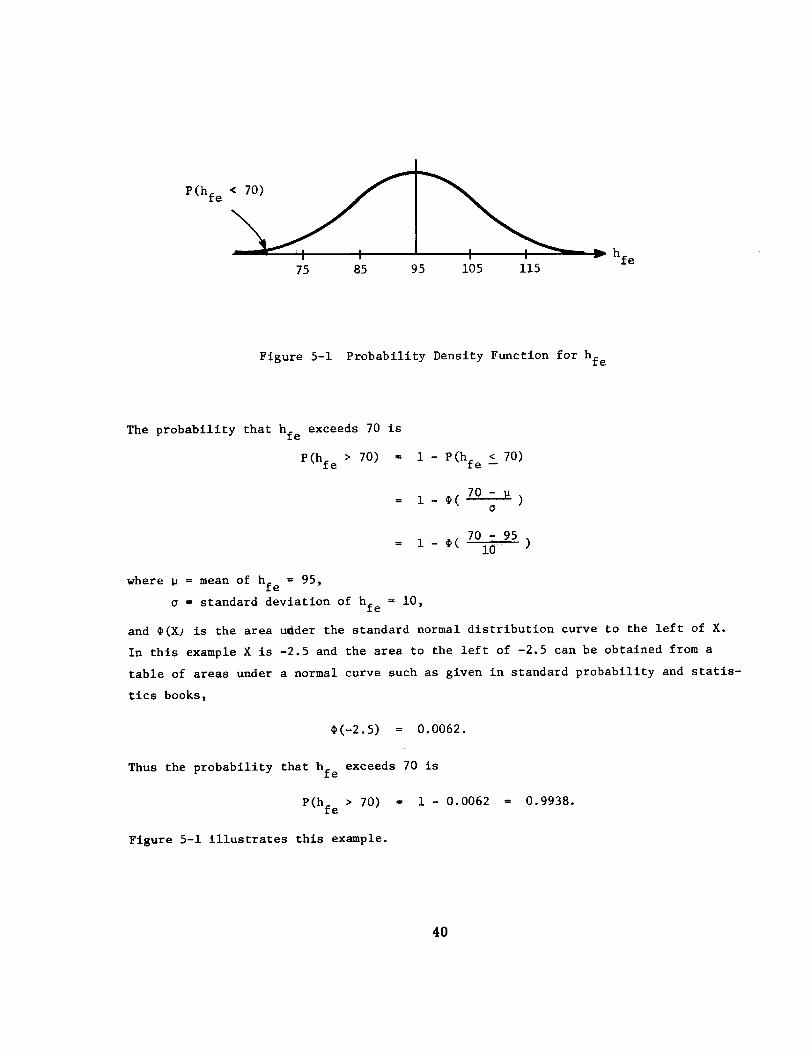
P(hfe
75 85 95 105 115hfe
Figure 5-1 Probability Density Function for hfe
The probability that hfe exceeds 70 is
P(hfe > 70) = i - P(hfe ! 70)
70-u L: i- _( - )
= 1 - _(
where _ : mean of hfe : 95,
o = standard deviation of hfe = i0,
and _(X) is the area udder the standard normal distribution curve to the left of X.
In this example X is -2.5 and the area to the left of -2.5 can be obtained from a
table of areas under a normal curve such as given in standard probability and statis-
tics books,
_(-2.5) : 0.0062.
Thus the probability that hfe exceeds 70 is
P(hfe > 70) : i - 0.0062 : 0.9938.
Figure 5-1 illustrates this example.
4O
The assumptions under which the above result was obtained are given below and should
be carefully noted when using these techniques:
(i) Normal distribution of values of hfe,
(2) Known mean and standard deviation, and
(3) Conditions of manufacture and operation of items are same as
those to which the probability estimate is to apply.
Checking the first and second assumption would depend on the source of the informa-
• tion for the hfe distribution. Often this will come from special tests for this
purpose. If so, the first assumption above can be checked graphically by plotting
the sample distribution function on normal probability paper. The extent to which
one can check the adequacy of the normality in the region of the tails depends upon
the amount of data. The second assumption is really never satisfied but for very
large sample sizes the results would be practically unaltered by using procedures
which depend on the sample mean x and standard deviation s. The third asst_ption is
of special importance to the design engineer in that he will specify the test condi-
tions to correspond as nearly as possible to those conditions under which he wishes
to infer the quality concerning the items tested.
Similar results can be obtained using other forms of distributions such as
log-normal, Weibull, extreme-value, etc. In each case the "goodness" of the distri-
bution can be checked by a probability graph of appropriate form and/or by analytical
techniques such as given in statistical texts, e.g. see Ref. 23.
5.3 Stress-Strength Model (Bound Distribution)
In this case the performance of an item is considered to be satisfactory if the
strength of the item exceeds the stress to which it is to be exposed in application.
Thus the bounds may not be fixed in that an item selected at random and used in a
specific system may be subjected to one of a distribution of stresses rather than
a known fixed stress. In actual practice the stress may vary over the life of the
item but consider for the moment that an item is subjected to a constant stress over
its life and that the stress level may vary from item to item.
The approach to this problem is to specify the stress and the strength density
functions by one of the methods of Appendix A.I. Then the parameters of the distri-
butlons are estimated and one then computes the estimate of the desired probability.
Thus in the notation suggested earlier, the strength density function is p(y) and
the stress by p(s). Then it is desired to determine the probability that y is larger
than s.
41
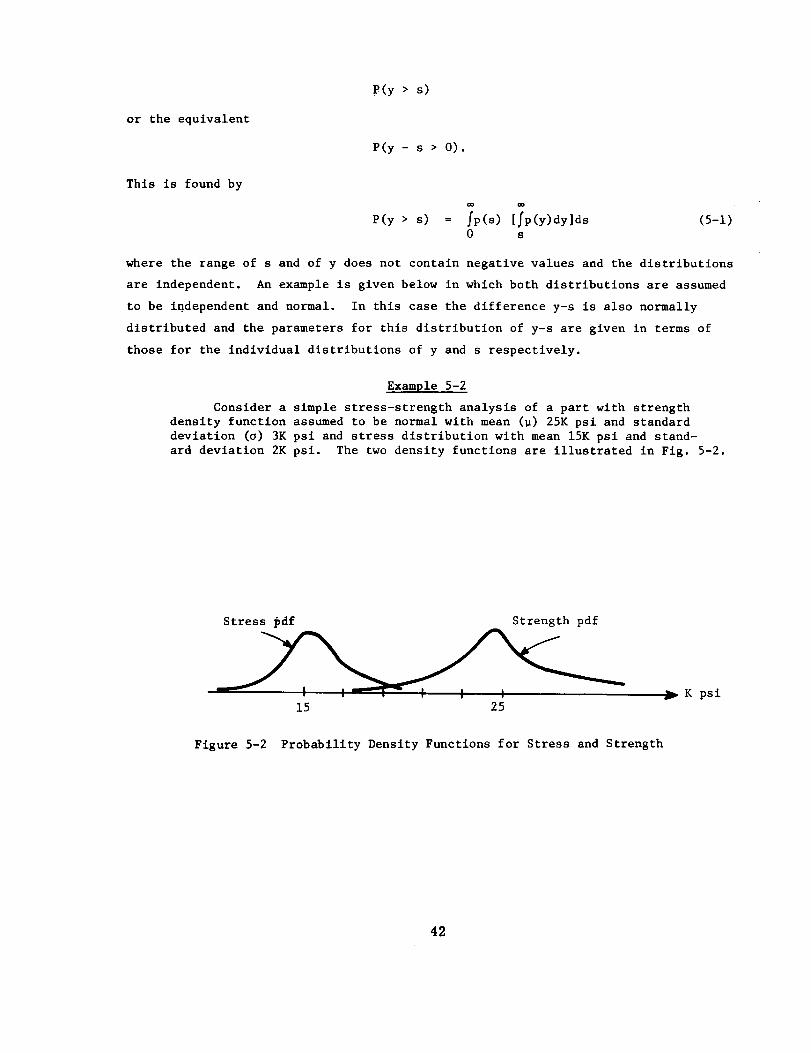
or the equivalent
This is found by
P(y > s)
P(y - s > 0).
P(y > s) = 7p(s) [Tp(y)dy]ds (5-i)
0 s
where the range of s and of y does not contain negative values and the distributions
are independent. An example is given below in which both distributions are assumed
to be independent and normal. In this case the difference y-s is also normally
distributed and the parameters for this distribution of y-s are given in terms of
those for the individual distributions of y and s respectively.
Example 5-2
Consider a simple stress-strength analysis of a part with strength
density function assumed to be normal with mean (_) 25K psi and standard
deviation (o) 3K psi and stress distribution with mean 15K psi and stand-
ard deviation 2K psi. The two density functions are illustrated in Fig. 5-2.
Stress _df Strength pdf
15 25K psi
Figure 5-2 Probability Density Functions for Stress and Strength
42
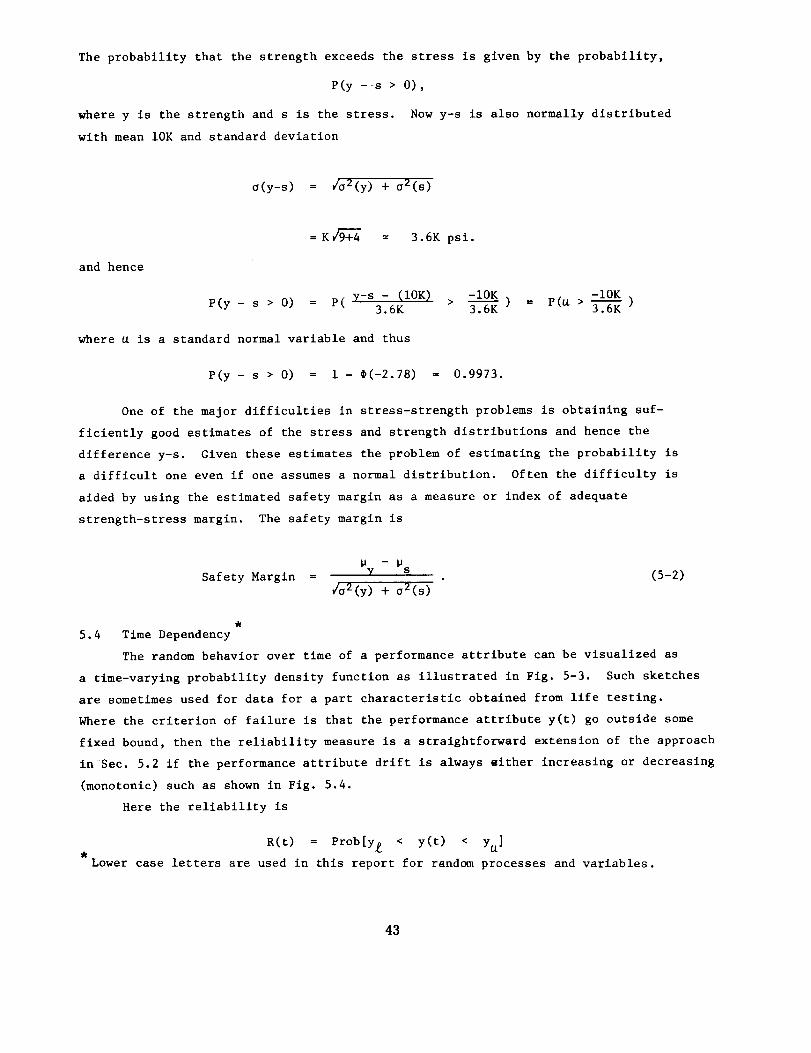
The probability that the strength exceeds the stress is given by the probability,
P(y - s > 0),
where y is the strength and s is the stress. Now y-s is also normally distributed
with mean 1OK and standard deviation
o(y-s) = /o2(y) + o2(s)
= K 9_ = 3.6K psi.
and hence
P(y - s > 0) = p( y-s - _IOK_3.6K
where u is a standard normal variable and thus
-10K -10K> 3.6K ) = P(u > _ )
P(y - s > 0) = 1 - @(-2.78) = 0.9973.
One of the major difficulties in stress-strength problems is obtaining suf-
ficiently good estimates of the stress and strength distributions and hence the
difference y-s. Given these estimates the problem of estimating the probability is
a difficult one even if one assumes a normal distribution. Often the difficulty is
aided by using the estimated safety margin as a measure or index of adequate
strength-stress margin. The safety margin is
- _SSafety Margin = Y (5-2)
/a2(y) + o2(s)
5.4 Time Dependency
The random behavior over time of a performance attribute can be visualized as
a time-varying probability density function as illustrated in Fig. 5-3. Such sketches
are sometimes used for data for a part characteristic obtained from life testing.
Where the criterion of failure is that the performance attribute y(t) go outside some
fixed bound, then the reliability measure is a straightforward extension of the approach
in Sec. 5.2 if the performance attribute drift is always either increasing or decreasing
(monotonic) such as shown in Fig. 5.4.
Here the reliability is
R(t) = Prob[y/ < y(t) < yu]
Lower case letters are used in this report for random processes and variables.
43
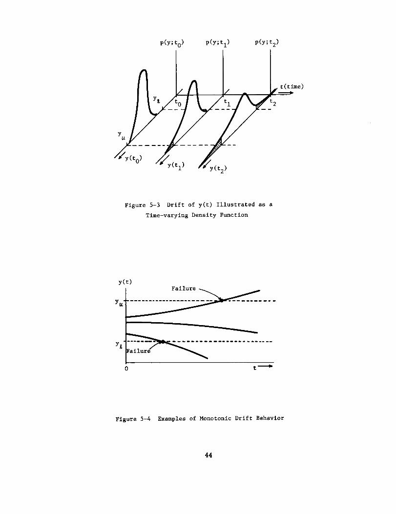
p(y;t0) P(Y;tl) P(Y;t2)
t(t__ _e)
t2
Figure 5-3 Drift of y(t) lllustrated as a
Time-varying Density Function
y(t)
Y_t'
t----_
0
Figure 5-4 Examples of Monotonic Drift Behavior
44
which is also
Yu
R(t) = f p(y; t)dy
Y£
where the integration is over y at time t and R(t) is a monotonically decreasing
function. An approximation to R(t) by performing this integration on the p(y; t)
at selected times t will often suffice. It is stressed that this approach is for a
monotonic drift. Non-monotonic drift such as shown in Fig. 5-5 introduces additional
considerations.
For non-monotonic drift first consider the failure criterion treated above where
failure is defined as the performance attribute going outside some fixed bound. If
all that is known is some p(y; t), then the drift reliability cannot be obtained.
For instance, the p(y; t) at time tI and at some later time t 2 might be identical,
but this does not mean that no additional failures have occurred because in a
population of items some which were out of bound may have drifted back in and others
may have drifted out. Therefore it is necessary to describe the time-varying
distributions of the performance attributes with a functional form. Here the
performance attribute is expressed as a deterministic function y(t) = y(£; t) where
the _ are probabilistic with known probability density p(_). This method can be
used where the drift failure criterion is a first crossing of a bound for either
monotonic or non-monotonic drift such as in the above discussions, and it also ban be
used for other criteria for non-monotonic drift such as the following:
(i) the cumulated area outside a bound(s),
(2) the number of crossings of a bound(s),
(3) the cumulated time outside a bound(s).
The approach for non-monotonic drift is to reduce the failure criterion to a first
crossing problem. A new function w(t) is defined such that reliability becomes
R(t) = P(y£ < w(t) < y_).
As an example, Fig. 5-5 illustrates the last failure criterion of the amount of time
that y_t) is outside the bounds. Here a corresponding function w(t) is defined, and
the failure criterion becomes w(t) first crossing a specified level w . Other w(t)
functions could be established for other failure criteria.
An example of a possible mathematical form for describing the performance
attribute is the polynomial expression y(t) = b 0 + b I t + ... + bn tn where the b's
are random variables of the same sign for monotonic drift and of mixed signs for
non-monotonic drift. Trigonometric series offer forms for periodically varying
attributes.
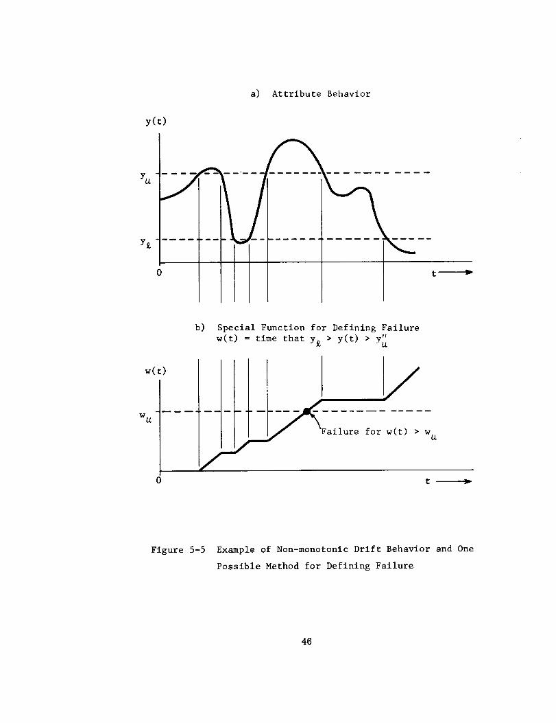
a) Attribute Behavior
y(t)
Y_
Y_
0
J
l
i
w_
b) Special Function for Defining Failure
w(t) : time that y_ > y(t) > v""' U.
w(t)
w u_ailure
/for w(t) > w u
0 t
Figure 5-5 Example of Non-monotonic Drift Behavior and One
Possible Method for Defining Failure
46
In some situations where the drift of the performance attribute is non-
monotonic it may be represented by a stochastic process. Such a situation could be
the error in a system output. For example, a stationary Markov Gaussian noise
process may be completely described by its auto-correlation function or its power
spectral density. An experimental application has been made using this general
approach for the error in a tilt stabilization assembly for an airborne radar antenna
[Ref. 24]. A recent theoretical book [Ref. 25] discusses various reliability
indices for stochastic processes.
The discussion in this section is about fixed-bounds. The reader who is
interested in time-dependent problems where the bound is a distribution (such as
in Sec. 5.3 for the stress-strength problem) would find some guidance in the
discussion of Part IV. The basic idea would be to treat both the performance
attribute and the bound as independent variables in a deterministic function. The
dependent variable then becomes a single performance attribute which has a fixed
bound for the failure criterion. For example, let w(t) = y(t) - s(t) where y is
the strength, s is the stress, and w is the new performance attribute which has
the bound w(t) > 0.
Two examples follow where the performance attribute is a time-varying normal
distribution. In these examples the performance attributes are of the form
y(t) = y(_; t) where the _ are normally distributed.
Example 5-3
Suppose that the resistance of a particular electrical resistor
changes over the interval 0 < t ! T according to
where
r(t) = Sl + a2 t ohms
_i is normal with mean 330_ and standard deviation 33_,
=2 is normal with mean -O.003_/hour and standard deviation
0.001_/hour.
47
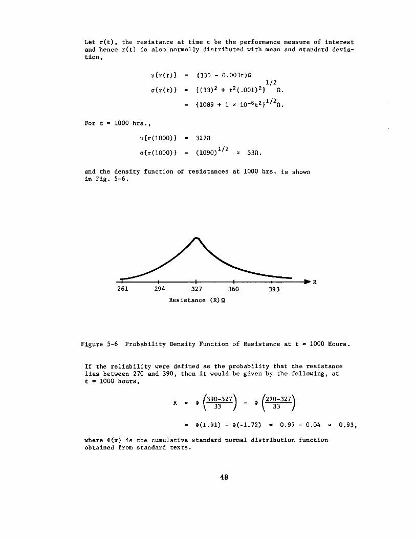
Let r(t), the resistance at time t be the performance measure of interest
and hence r(t) is also normally distributed with mean and standard devia-
tion,
_{r(t)} =
a{r(t)} =
5330 - 0.003t)_
1/2
{(33) 2 + t2(.001) 2} n.
{1089 + 1 × lO-6t2}i/2n.
For t = 1000 hrs.,
u{r(1000)} = 327n
o{r(lO00)} = (1090) 1/2 -" 33R.
and the density function of resistances at i000 hrs. is shown
in Fig. 5-6.
261 294 327 360 393
Resistance (R)
Figure 5-6 Probability Density Function of Resistance at t = I000 Hours.
If the reliability were defined as the probability that the resistance
lies between 270 and 390, then it would be given by the following, at
t = 1000 hours,
= _(1.91) - _(-1.72) = 0.97 - 0.04 = 0.93,
where @(x) is the cumulative standard normal distribution function
obtained from standard texts.
48
Example 5-4
Suppose that a mechanical part under consideration has a strength
which decreases with time in accordance with some function of time under
stress. Let the strength be described by
y(t) = _i e-kt + _2(l-e-kt)
where e_ is the initial strength, _2 the strength as t-_, k is aconstan_ determined by the particular part. Let also
_i be normally distributed with mean 50K psi andstandard deviation 4K psi,
_2 be normally distributed with mean 20K psi,
standard deviation 2K psi and assume that
it is correlated with y(0), i.e. p = 0.90,
and
k = 0.001.
Thus y(t) is also normally distributed with mean
-0.001t -.001t)]_{y(t)} = [50K e + 20K(l-e psi,
and standard deviation
-0.002t .001t)2o{y(t)} = {42K 2 e + (l-e- 22K 2
-0.001t+ 2(0.90) e 4K • 2K(l-e-0"001t)}i/2psi
= K{5.6e -0"002t + 6.4 -'001t + 4}i/2psi.
For t = i000 cycles, _{y(t)} = 31,000 and o{y(t)} = 2670. If the
prescribed lower limit were yf = 30K psi, what is the maximum numberof cycles to which the part sNould be exposed in order that the
probability of its strength exceeding 30,000 psi will be 0.95?
To solve this problem we must find t such that
_{y(t)} - 1.645 • o{y(t)} = 30,000
-0.001t -.001t)50K e + 20K(1-e - 1.645K [5.6e -0"002t + 6.4e -0" 001t + 4]1/2
- 30K = 0.
By graphing the left member of the above equation one can estimate
the time t at which the curve crosses the axis and hence obtain a
more exact solution analytically if desired.
49
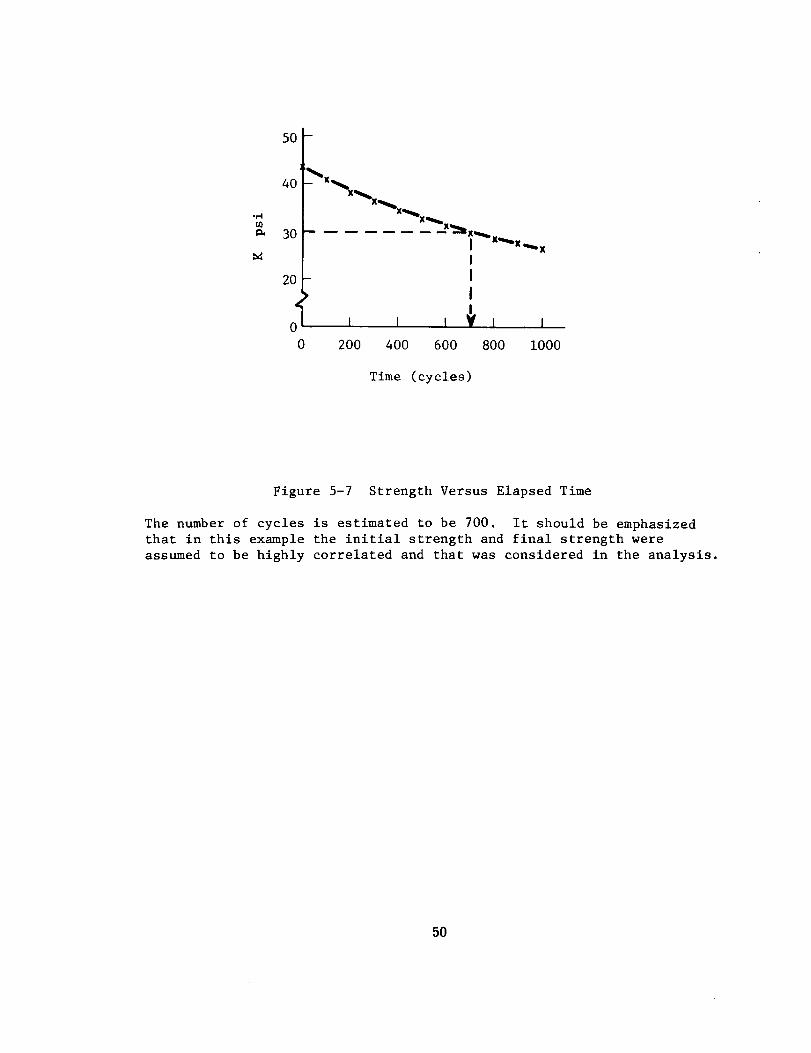
40["x...
"_ 30 x_x"x"_--x_.x.. _
20
0
0
I I
200 400
I
lI
|
600 800 i000
Time (cycles)
Figure 5-7 Strength Versus Elapsed Time
The number of cycles is estimated to be 700. It should be emphasized
that in this example the initial strength and final strength were
assumed to be highly correlated and that was considered in the analysis.
5O
6.0 Numerical Index Values
Guidance is given in this section for obtaining numerical values to be used
for the various single item reliability indexes which were introduced in Secs. 4 and 5.
Numerical index values (or data as they are sometimes referred to) result from actual
measurements, either from operational use or from testing. Reliability index measure-
ment is at best difficult. Most attempts at it suffer from lack of precision in the
failure criteria, in recording the operating conditions, and in knowledge of the
history of use of the item. It is desirable to keep in mind such loose conditions
under which the data for most reliability indexes was obtained so as not to exaggerate
their accuracy.
6.1 Comprehensive Guide
A recent Navy-sponsored effort to identify reliability data sources gives
elaboration on sources of reliability data and specific information regarding where
to direct inquiries [Ref. 26]. This is a comprehensive guide and identifies many
sources for direct reliability indexes as well as for supporting reliability data.
6.2 Reliability Measure Sources
Index values for failure rates and other reliability measures as were identified
in Sec. 4 are treated here. Almost universally these data are for an assumed constant
failure rate for nonrepairable items and for an assumed mean-time-between-failure of
the Poisson process for repairable items.
MIL HDBK 217A. This is a widely used and generally available source. Typically
the failure rate of the nonrepairable item is for an electronic part and is shown
graphically as a function of several stresses, with additional multipliers to be used
for different classes of operational use. The latest revision of this is dated
December i, 1965, and is revision A [Ref. 27]; however, as of this date another
revision is in process.
MTBF Estimating Relationships. Simple MTBF estimating relationships have been
developed for electronic equipment and are quite useful for preliminary predictions.
Here the independent variables may simply be the number of active elements and the
usage class of the equipment [Refs. 2 and 27].
FARADA. The focal point of reliability data is the Failure Rate Data (FARADA)
program which is sponsored by the Tri-service and NASA in cooperation with qualified
government contractors. This program is currently conducted by the Naval Fleet
Missile Systems Analysis and Evaluation Group (FMSAEG) at Coronado, California
[Ref. 28]. Data inputs from hundreds of sources are collected, compiled and distri-
buted. The primary distribution is in the form of a series of handbooks.
51
Reliability Analysis Central. The Air Force Rome Air Development Center is
currently developing a Reliability Analysis Central which is planned to become fully
operational by mid 1969 [Ref. 29]. The Central is to serve as the Air Force focal
point for reliability data.
Non-electronic Data. The data sources noted to this point in Sec. 6.2 are
primarily electronic in nature. Generally there is more electronic data than for
other con_nodities and failure causes. Some compilation of non-electronic reliability
data are Refs. 30 and 31 sponsored respectively by the Navy and Air Force. The
Air Force-sponsored work is still in progress.
6.3 Bound-Crossing Data
Distribution information to be used with the bound-crossing type of reliability
measure of Sec. 5 is con_nented on below. The degradation type of failure mode is
often not explicitly considered in reliability predictions for electronic items, and
there are few established data sources for this failure mode. The FARADA program
and the developing RADC Reliability Analysis Central include degradation and drift
data under their scope of activity, though not much data are yet included. Equipment
and system producers who perform degradation studies have, of course, compiled some
numerical information. Sometimes this is made publicly available to others [Ref. 32].
Non-electronic reliability predictions of the bound-crossing variety are principally
the stress-strength problem. An Air Force-sponsored compilation of appropriate data
for such predictions has been recently published [Ref. 33]. The data here are
primarily for distributions of fatigue strength of various mechanical material.
6.4 Remarks
An undesirable feature of currently available data is that too often it is a
matter of collecting and passing on what has been reported without very much analysis.
One reason for this is that the inputs coming into these collection points are often
lacking in supporting information so that analysis is not possible. As the previously
mentioned FARADA program continues to progress and as the Reliability Analysis Central
becomes established, it can be expected that there will be more screening and analysis
on what is ultimately made generally available. An example of the type of data col-
lecting and analysis which is desirable was recently performed for NASA and was
concerned with historical reliability data from inflight spacecraft [Ref. 34].
Many equipment suppliers are currently collecting and analyzing reliability
data on equipment which they have produced. This sort of data collection effort is
extremely desirable and is to be encouraged. If the samples from which such data are
drawn are of sufficient quantity, the opportunity exists for developing data that can
be drawn on by the equipment suppliers to give more precise results.
52

The person who is interested in reliability data should keep his eye open in
the general literature. Occasionally a paper or report will contain preliminary data
of the sort which is not in the established data sources. As an example, consider
the human failure mode. A recent paper remarked that a certain percentage of actual
failures were found to be caused by human error [Ref. 35]. Certain reliability pre-
dictions would be better off to include such failure modes with best available index
values rather than to omit them.
53
Part III: Multi-Item Problems
Various approaches for developing reliability prediction equations for system
reliability as functions of item reliabilltles and other variables are presented.
These are the conventional and classical ones which are suitable for practical
applications. Inputs to these equations are the single item reliability definitions
from Part I.
Section 7 covers logic models, time is explicitly brought into consideration
in Sec. 8, and Sec. 9 covers the influence of environments which are known probabilis-
tlcally and bound-crosslng problems. This material will, to varying extents, be
old-hat to experienced reliability analysts. However, some of it is not stressed
in existing reliability analysis handbooks or books; including the following: In
Sec. 7 are the use of cuts and paths for developing prediction models for complex
configurations and the problem of models for multl-phase missions. In Sec. 8 the
extreme value approach is discussed in a general manner and a general reliability
prediction model is derived (first known publication). In Sec. 9 are discussions
of the influence of environment which is known probabillstlcally and a specific
application of this to the multl-ltem stress-strength problem.
Reliability prediction equations have the apparent use of providing a nomerlcal
reliability prediction index for a proposed system configuration. Although the details
contained in this report explicitly cover only this use, it is well to be aware of
other applications. These include: Using the model for sensitivity studies in order
to study the results of changes in input parameters by either limit or probabillstic
approaches. An approach could involve application of the method of moments such as
cited in Sec. 9.3.1 for a different problem. Another use is to provide part of the
equations needed for the application of literal optimization approaches to reliability
allocation problems. This use prompted the derivation of the general redundancy model
of Sec. 8.4. Yet another use is that certain practical engineering guidelines can be
gleaned from studying the models. An instance of this is the outline at the end of
Sec. 9.2 for multi-ltem stress-strength problems.
It should also be noted that the discussions of Secs. 7, 8, and 9 are oriented
mainly toward bringing items together into a system. These modeling concepts are,
of course, the same ones which would be utilized for bringing detailed failure-modes
together, where an item might have multiple failure modes such as were acknowledged
in Secs. 4.1 and 4.3. Some treatment of modes will be given in Sec. 7.6 on N-state
logic models and in Sec. 9.1 on the general question of the influence of environment.
Part IV will pursue detailed consideration of failure modes.
54
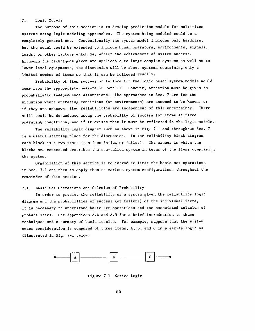
7. Logic Models
The purpose of this section is to develop prediction models for multi-ltem
systems using logic modeling approaches. The system being modeled could be a
completely general one. Conventionally the system model includes only hardware,
but the model could be extended to include human operators, environments, signals,
loads, or other factors which may affect the achievement of system success.
Although the techniques given are applicable to large complex systems as well as to
lower level equipments, the discussion will be about systems containing only a
limited number of items so that it can be followed readily.
Probability of item success or failure for the logic based system models would
come from the appropriate measure of Part II. However, attention must be given to
probabillstic independence assumptions. The approaches in Sec. 7 are for the
situation where operating conditions (or environments) are assumed to be known, or
if they are unknown, item reliabilities are independent of this uncertainty. There
still could be dependence among the probability of success for items at fixed
operating conditions, and if it exists then it must be reflected in the logic models.
The reliability logic diagram such as shown in Fig. 7-1 and throughout Sec. 7
is a useful starting place for the discussion. In the reliability block diagram
each block is a two-state item (non-failed or failed). The manner in which the
blocks are connected describes the non-failed system in terms of the items comprising
the system.
Organization of this section is to introduce first the basic set operations
in Sec. 7.1 and then to apply them to various system configurations throughout the
remainder of this section.
7.1 Basic Set Operations and Calculus of Probability
In order to predict the reliability of a system given the reliability logic
diagrmm and the probabilities of success (or failure) of the individual items,
it is necessary to understand basic set operations and the associated calculus of
probabilities. See Appendices A.4 and A.5 for a brief introduction to these
techniques and a summary of basic results. For example, suppose that the system
under consideration is composed of three items, A, B, and C in a series logic as
illustrated in Fig. 7-1 below.
° l v y
Figure 7-1 Series Logic
55
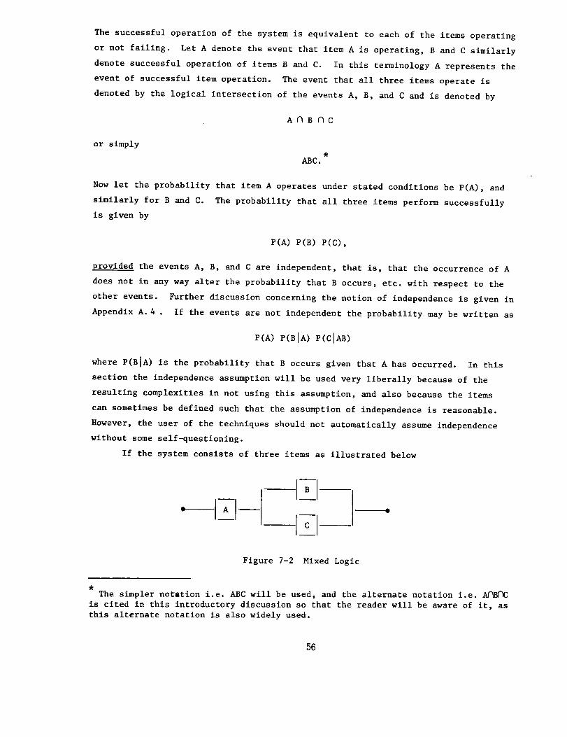
The successful operation of the system is equivalent to each of the items operating
or not failing. Let A denote the event that item A is operating, B and C similarly
denote successful operation of items B and C. In this terminology A represents the
event of successful item operation. The event that all three items operate is
denoted by the logical intersection of the events A, B, and C and is denoted by
ANBNC
or simply
ABC.
Now let the probability that item A operates under stated conditions be P(A), and
similarly for B and C. The probability that all three items perform successfully
is given by
P(A) P(B) P(C),
provided the events A, B, and C are independent, that is, that the occurrence of A
does not in any way alter the probability that B occurs, etc. with respect to the
other events. Further discussion concerning the notion of independence is given in
Appendix A. 4 . If the events are not independent the probability may be written as
P(A) P(BIA ) P(CIAB )
where P(BIA ) is the probability that B occurs given that A has occurred. In this
section the independence assumption will be used very liberally because of the
resulting complexities in not using this assumption, and also because the items
can sometimes be defined such that the assumption of independence is reasonable.
However, the user of the techniques should not automatically assume independence
without some self-questioning.
If the system consists of three items as illustrated below
Figure 7-2 Mixed Logic
The simpler notation i.e. ABC will be used, and the alternate notation i.e. AfIB(]C
is cited in this introductory discussion so that the reader will be aware of it, as
this alternate notation is also widely used.
56
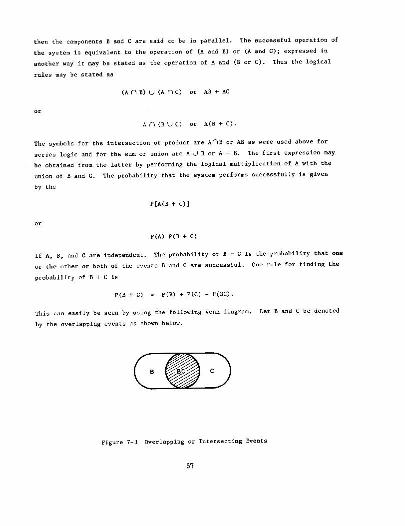
then the components B and C are said to be in parallel. The successful operation of
the system is equivalent to the operation of (A and B) or (A and C); expressed in
another way it may be stated as the operation of A and (B or C). Thus the logical
rules may be stated as
(A (_ B) _9 (A (_C) or AB + AC
or
A(_ (BUC) or A(B + C).
The symbols for the intersection or product are Af_B or AB as were used above for
series logic and for the sum or union are AUB or A + B. The first expression may
be obtained from the latter by performing the logical multiplication of A with the
union of B and C. The probability that the system performs successfully is given
by the
P[A(B + C)]
or
P(A) P(B + C)
if A, B, and C are independent. The probability of B + C is the probability that one
or the other or both of the events B and C are successful. One rule for finding the
probability of B + C is
P(B + C) = P(B) + P(C) - F(BC).
This can easily be seen by using the following Venn diagram. Let B and C be denoted
by the overlapping events as shown below.
Figure 7-3 Overlapping or Intersecting Events
57
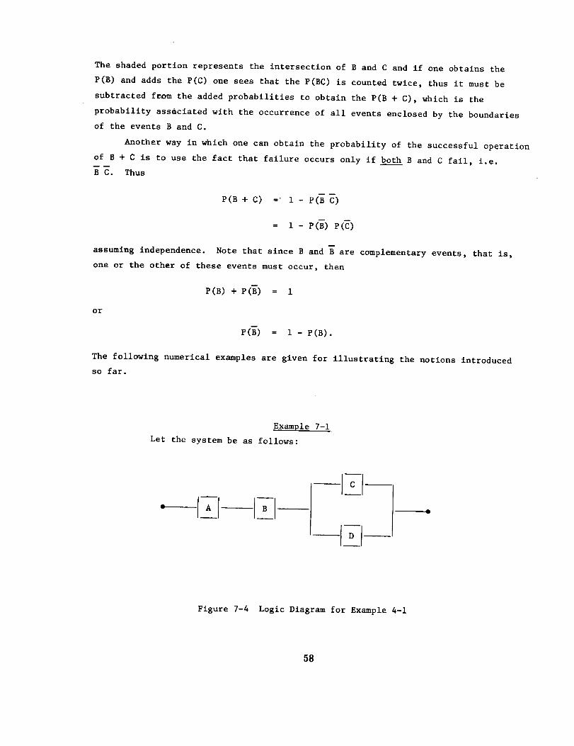
The shaded portion represents the intersection of B and C and if one obtains the
P(B) and adds the P(C) one sees that the P(BC) is counted twice, thus it must be
subtracted f_om the added probabilities to obtain the P(B + C), which is the
probability ass_clated with the occurrence of all events enclosed by the boundaries
of the events B and C.
Another way in which one can obtain the probability of the successful operation
of B + C is to use the fact that failure occurs only if both B and C fail, i.e.
B C. Thus
P(B + C) =" i - P(B C)
= 1 - F(B) e(_)
assuming independence. Note that since B and B are complementary events, that is,
one or the other of these events must occur, then
P(B) + P(B) -- 1
or
P(B) = i - P(B).
The following numerical examples are given for illustrating the notions introduced
so far.
E_ample 7-i
Let the system be as follows:
Figure 7-4 Logic Diagram for Example 4-1
58
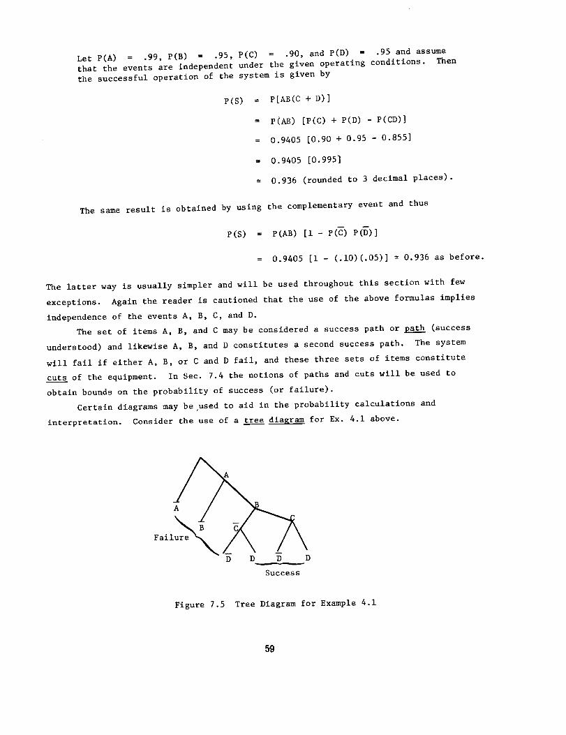
Let P(A) = .99, P(B) = .95, P(C) = .90, and P(D) = .95 and assume
that the events are independent under the given operating conditions. Then
the successful operation of the system is given by
P(S) = P[AB(C + D)]
= P(AB) [P(C) + P(D) - P(CD)]
= 0.9405 [0.90 + 0.95 - 0.855]
= 0.9405 [0.995]
= 0.936 (rounded to 3 decimal places).
The same result is obtained by using the complementary event and thus
P(S) = P(AB) [I - P(_) P(D) ]
= 0.9405 [i - (.10)(.05)] = 0.936 as before.
The latter way is usually simpler and will be used throughout this section with few
exceptions. Again the reader is cautioned that the use of the above formulas implies
independence of the events A, B, C, and D.
The set of items A, B, and C may be considered a success path or path (success
understood) and likewise A, B, and D constitutes a second success path. The system
will fail if either A, B, or C and D fail, and these three sets of items constitute
cuts of the equipment. In Sec. 7.4 the notions of paths and cuts will be used to
obtain bounds on the probability of success (or failure).
Certain diagrams may be used to aid in the probability calculations and
interpretation. Consider the use of a tree diagram for Ex. 4.1 above.
A A
Fail
D D D D
Success
Figure 7.5 Tree Diagram for Example 4.1
59
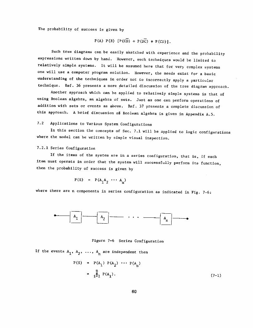
The probability of success is given by
P(A) P(B) [P(CD) + P(D_) + P(CD)].
Such tree diagrams can be easily sketched with experience and the probability
expressions written down by hand. However, such techniques would be limited to
relatively simple systems. It will be assumed here that for very complex systems
one will use a computer program solution. However, the needs exist for a basic
Understanding of the techniques in order not to incorrectly apply a particular
technique. Ref. 36 presents a more detailed discussion of the tree diagram approach.
Another approach which can be applied to relatively simple systems is that of
using Boolean algebra, an algebra of sets. Just as one can perform operations of
addition with sets or events as above. Ref. 37 presents a complete discussion of
this approach. A brief discussion o_ Boolean algebra is given in Appendix A.5.
7.2 Applications to Various System Configurations
In this section the concepts of Sec. 7.1 will be applied to logic configurations
where the model can be written by simple visual inspection.
7.2.1 Series Configuration
If the items of the system are in a series configuration, that is, if each
item must operate in order that the system will successfully perform its function,
then the probability of success is given by
P(S) = P(AIA 2 "'" An )
where there are n components in series configuration as indicated in Fig. 7-6:
Figure 7-6 Series Configuration
If the events AI, A2, ..., An are independent then
P(S) = P(A I) P(A 2) "°" P(A n)
n
-- illl P(Ai). (7-1)
B0
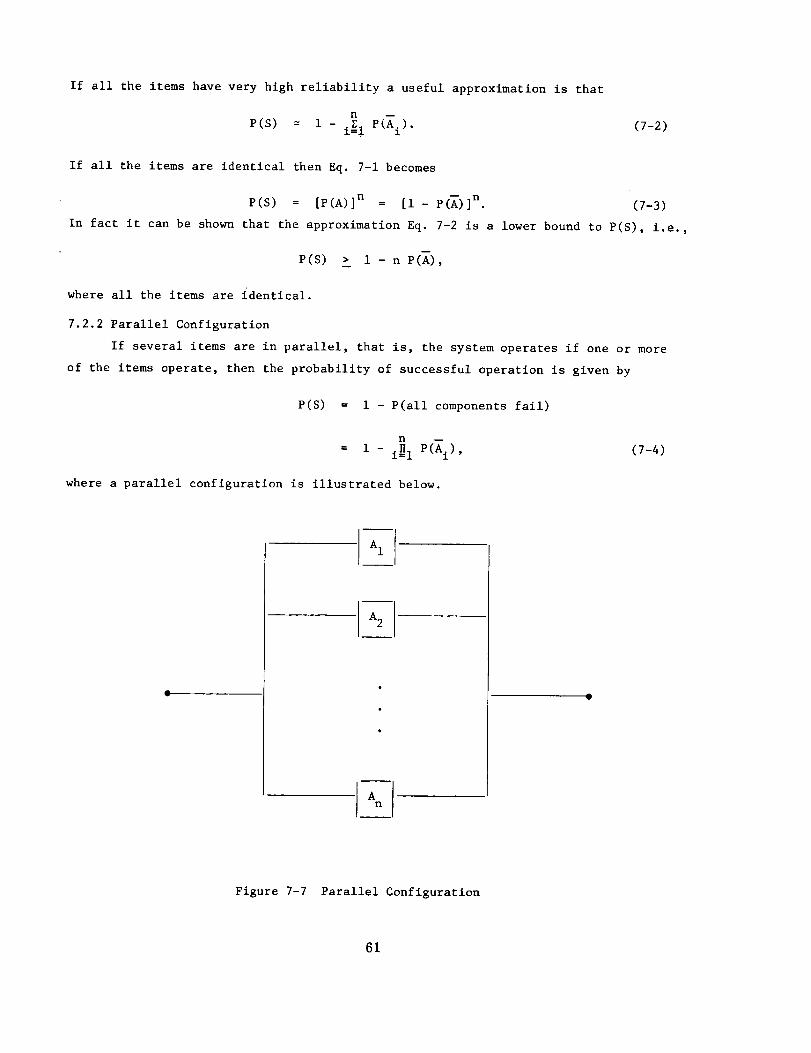
If all the items have very high reliability a useful approximation is that
n
P(S) = 1 - i_l P(_i )" (7-2)
If all the items are identical then Eq. 7-1 becomes
P(S) = [P(A)] n = [i - P(A)] n. (7-3)
In fact it can be shown that the approximation Eq. 7-2 is a lower bound to P(S), i.e.,
P(S) > 1 - n P(A),
where all the items are identical.
7.2.2 Parallel Configuration
If several items are in parallel, that is, the system operates if one or more
of the items operate, then the probability of successful operation is given by
P(S) = i - P(all components fail)
n
= 1 - i_ 1 P(Ai) , (7-4)
where a parallel configuration is illustrated below.
Figure 7-7 Parallel Configuration
61
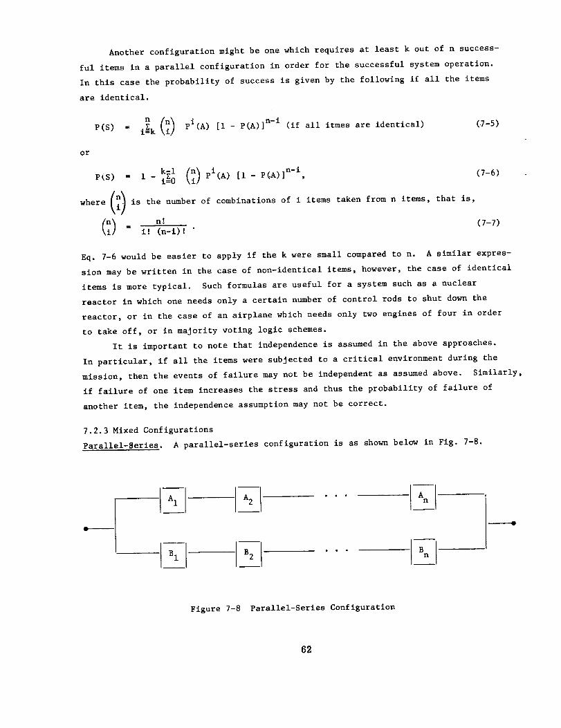
Another configuration might be one which requires at least k out of n success-
ful items in a parallel configuration in order for the successful system operation.
In this case the probability of success is given by the following if all the items
are identical.
or
P(S) = iEk pi(A) [i - P(A)] n-i (if all itmes are identical) (.7-5)
PiS) -- 1 - i$0 (A) [i - P(A)] n-i, (7-6)
where(i ) is the number of combinations of i items taken from n items, that is,% I
o- i! (n-i)! " (7-7)
Eq. 7-6 would be easier to apply if the k were small compared to n. A similar expres-
sion may be written in the case of non-identical items: however, the case of identical
items is more typical. Such formulas are useful for a system such as a nuclear
reactor in which one needs only a certain number of control rods to shut down the
reactor, or in the case of an airplane which needs only two engines of four in order
to take off, or in majority voting logic schemes.
It is important to note that independence is assumed in the above approaches.
In particular, if all the items were subjected to a critical environment during the
mission, then the events of failure may not be independent as assumed above. Similarly,
if failure of one item increases the stress and thus the probability of failure of
another item, the independence assumption may not be correct.
7.2.3 Mixed Configurations
Parallel-Series. A parallel-series configuration is as shown below in Fig. 7-8.
Figure 7-8 Parallel-Series Configuration
82
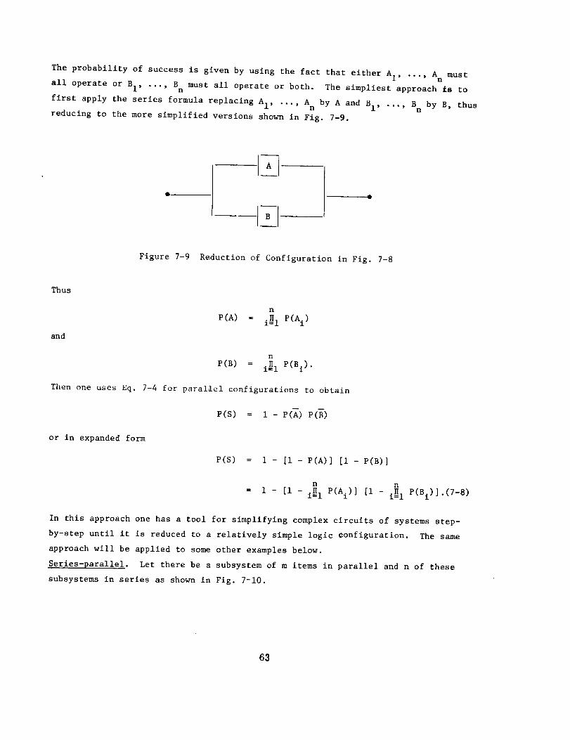
, o mu8 tThe probability of success is given by using the fact that either A I .., A n
all operate or BI, ..., Bn must all operate or both. The simpliest approach is to
first apply the series formula replacing AI, ... A by A and BI, ... B n by B, thusn
reducing to the more simplified versions shown in Fig. 7-9.
Figure 7-9 Reduction of Configuration in Fig. 7-8
Thus
and
n
P(A) -- i_l P(Ai)
n
P(B) = i_l P(Bi)"
Then one uses Eq. 7-4 for parallel configurations to obtain
P(S) = I - P(A) P(B)
or in expanded form
P(S) = i - [i - P(A)] [i - P(B)]
n n
= 1 - [i - i_ 1 V(Ai)] [i - i_l P(Bi)]'(7-8)
In this approach one has a tool for simplifying complex circuits of systems step-
by-step until it is reduced to a relatively simple logic configuration. The same
approach will be applied to some other examples below.
Series-parallel. Let there be a subsystem of m items in parallel and n of these
subsystems in series as shown in Fig. 7-10.
63
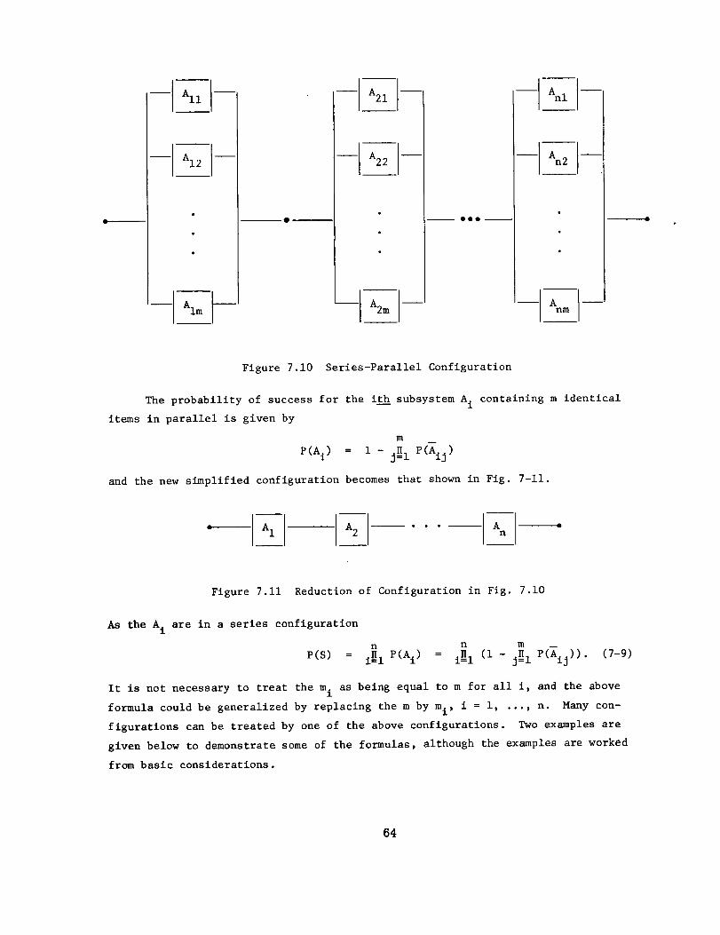
-- 000
Figure 7.10 Series-Parallel Configuration
The probability of success for the it__h_hsubsystem A i containing m identical
items in parallel is given by
m
P(A i) = 1 - J_l P(Aij)
and the new simplified configuration becomes that shown in Fig. 7-11.
Figure 7.11 Reduction of Configuration in Fig. 7.10
As the A i are in a series configuration
n n m
P(S) = i_l P(Ai) = i_l (i - J_l P(Aij ))" (7-9)
It is not necessary to treat the m i as being equal to m for all i, and the above
formula could be generalized by replacing the m by m i, i = i, ..., n. Many con-
figurations can be treated by one of the above configurations. Two examples are
given below to demonstrate some of the formulas, although the examples are worked
from basic considerations.
64
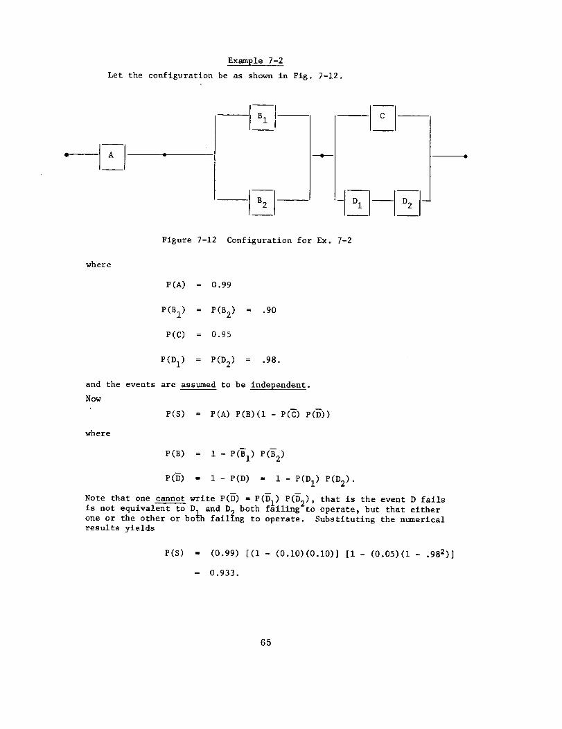
Example 7-2
Let the configuration be as shown in Fig. 7-12.
where
-- DI -- D 2 --P_ _IFigure 7-12 Configuration for Ex. 7-2
P(A) = 0.99
P(B I) -- P(B 2) = .90
P(C) = 0.95
P(D I) -- P(D 2) = .98.
and the events are assumed to be independent.
Now
P(S) = P(A) P(B)(I- P(C) P(D))
where
P(B) = I - P(B 1) P(B2)
P(D) = i - P(D) = 1 - P(DI) P(D2).
Note that one cannot write P(D) = P(D_) P(D--_), that is the event D fails
is not equivalen---_-_o D. and D^ both f_iling_to operate, but that either
one or the other or bob fail_ng to operate. Substituting the numerical
results yields
P(S) = (0.99) [(i - (0.i0)(0.i0)] [i - (0.05)(1 - .982)]
= 0.933.
65
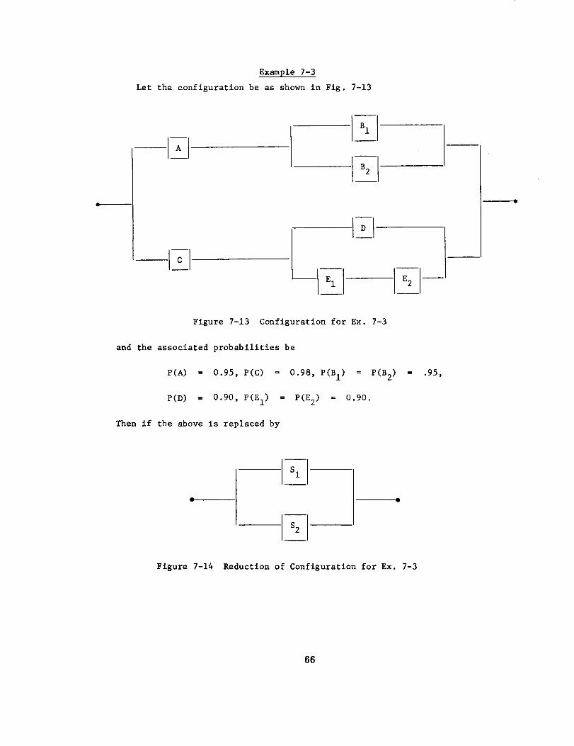
Example 7-3
Let the configuration be as shown in Fig. 7-13
Figure 7-13 Configuration for Ex. 7-3
and the associated probabilities be
P(A) 1 0.95, P(C) = 0.98, P(B 1) = P(B 2) = .95,
P(D) = 0.90, P(EI) = P(E 2) = 0.90.
Then if the above is replaced by
Figure 7-14 Reduction of Configuration for Ex. 7-3
86
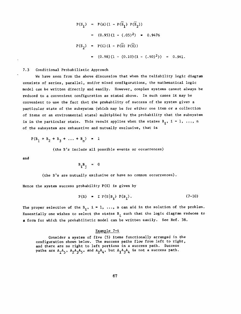
-- D
P(S I) = P(A)(I - P(B I) P(B2))
= (0.95)(1 - (.05) 2) = 0.9476
P(S 2) = P(C)(I - P(D) P(E))
= (0.98)(1 - (0.10)(1 - (.90)2)) = 0.961.
7.3 Conditional Probabillstlc Approach
We have seen from the above discussion that when the reliability logic diagram
consists of series, parallel, and/or mixed configurations, the mathematical logic
model can be written directly and easily. However, complex systems cannot always be
reduced to a convenient configuration as stated above. In such cases it may be
convenient to use the fact that the probability of success of the system given a
particular state of the subsystem (which may be for either one item or a collection
of items or an environmental state) multiplied by the probability that the subsystem
is in the particular state. This result applies when the states Bi, i = i, ..., n
of the subsystem are exhaustive and mutually exclusive, that is
and
P(B I + B 2 + B 3 + ... + Bn) = i
(the B's include all possible events or occurrences)
BIB j = 0
(the B's are mutually exclusive or have no common occurrences).
Hence the system success probability P(S) is given by
P(S) = E P(SIB i) P(BI). (7-10)
The proper selection of the B i, i = i, ..., n can aid in the solution of the problem.
Essentially one wishes to select the states B i such that the logic diagram reduces to
a form for which the probabilistic model can be written easily. See Ref. 38.
Example 7-4
Consider a system of five (5) items functionally arranged in the
configuration shown below. The success paths flow from left to right,
and there are no right to left portions in a success path. Success
paths are AIA5, A2A3A 5, and A2A4, but AIA3A 4 is not a success path.
67
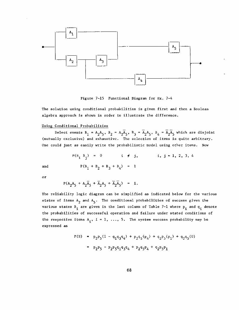
vFigure 7-15 Functional Diagram for Ex. 7-4
The solution using conditional probabilities is given first and then a Boolean
algebra approach is shown in order to illustrate the difference.
Usin$ Conditional Probabilities
Select events B 1 = A2A5, B 2 = A2A5, B 3 = A2A5 , B 4 = A2A 5 which are disjoint
(mutually exclusive) and exhaustive. The selection of items is quite arbitrary.
One could just as easily write the probabilistic model using other items. Now
and
P(B i Bj) = 0 i # J,
P(B I + B 2 + B3 + B 4) = i
i, j --i, 2, 3, 4
or
P(A2A 5 + A2A 5 + A2A5 + A2A 5) = i.
The reliability logic diagram can be simplified as indicated below for the various
states of items A 2 and A5. The conditional probabilities of success given the
various states B i are given in the last column of Table 7-1 where Pi and qi denote
the probabilities of successful operation and failure under stated conditions of
the respective items Ai, i = i, ..., 5. The system success probability may be
expressed as
P(S) = p2P5(l - qlq3q4 ) + p2q5(P4 ) + q2P5(Pl ) + q2q5(0)
= p2P5 - p2PSqlq3q 4 + P2q5P4 + q2P5Pl
68
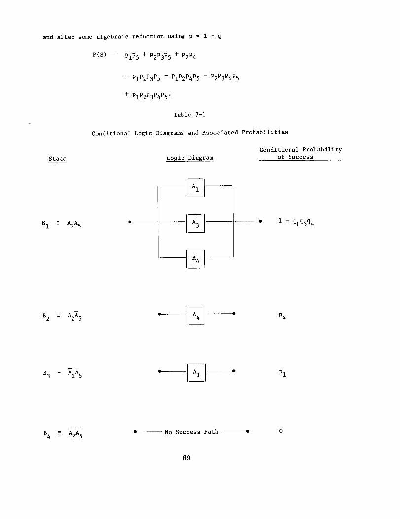
and after some algebraic reduction using p = 1 - q
P(S) = plP5 + p2P3P5 + p2P4
State
- plP2P3P5 - plP2P4P5 - p2P3P4P5
+ PlP2P3P4P 5.
Table 7-1
Conditional Logic Diagrams and Associated Probabilities
Conditional Probability
Logic Diagram of Success
B I E A2A 5 _- i - qlq3q4
B 2 - A2A 5 -" A4 -- P4
B3 E A2A5 -- _--i -- Pl
B 4 _ A2A 5e No Success Path ; 0
69

Usln_ Boolean Al_ebra
The Boolean algebra success model is
P(S) = P{AIA 5 + Am[A3A 5 + A4] }
= P_AIA 5 + AmA3A 5 + A2A41 •
and expanding using Theorem 4 of Appendix 4 and substituting the item success
probabilities p will yield the same results as were obtained above using conditional
probabilities.
7.4 Models Using Cuts and Paths
The concept of cut sets and success paths (or tie sets) offers another approach
to the development of reliability prediction models for systems having complexities.
In particular this approach is advantageous where the same item may appear more than
once in the reliability block diagram. Such a situation could arise where a system
must perform a n_nber of functions but some items are used in more than one function.
Here a different reliability logic diagram could be prepared for each function where
the same item will appear more than once. Another situation could arise where
different functions are to be performed by the system during subsequent mission
phases, thus leading to a different reliability logic diagram for each phase where
the same item will appear more than once. The cuts and paths approach can be used
to obtain an exact model, but this will usually be quite involved and the advantage
is that an approximate model can be readily developed. The more important results
are given in this section as derived in Ref. 39. The system reliability is
defined as the probability of successful function of all of the items in at least
one tie set or the probability that all cut sets are good. A tie set or success
path is a directed path from input to output as indicated in the simple system in
Fig. 7-16A. The tie sets or success paths are 2, 5; i, 3, 5; and I, 4, 5, respectively.
A cut set is a set of items which literally cuts all success paths or tie sets.
One is normally interested in the minimal cut set; i.e., the smallest or minimal set
of items such that the elimination of any one item would no longer make it a cut.
This is because a nonmlnimal cut set corresponds to more item failures than are
required to cause system failure. In the above example the minimal cut sets are
i, 2; 2, 3, 4; 5. Note that I, 5 is not a minimal cut set since 5 is already a cut
set and is a subset of i, 5. A cut set cuts the llne of communication between input
and output. A cut set is good if at least one of its elements is operative. The
system failure probability or system unreliability is the probability that all tie
sets are bad (a tie set is bad if at least one item fails) or the probability that
70
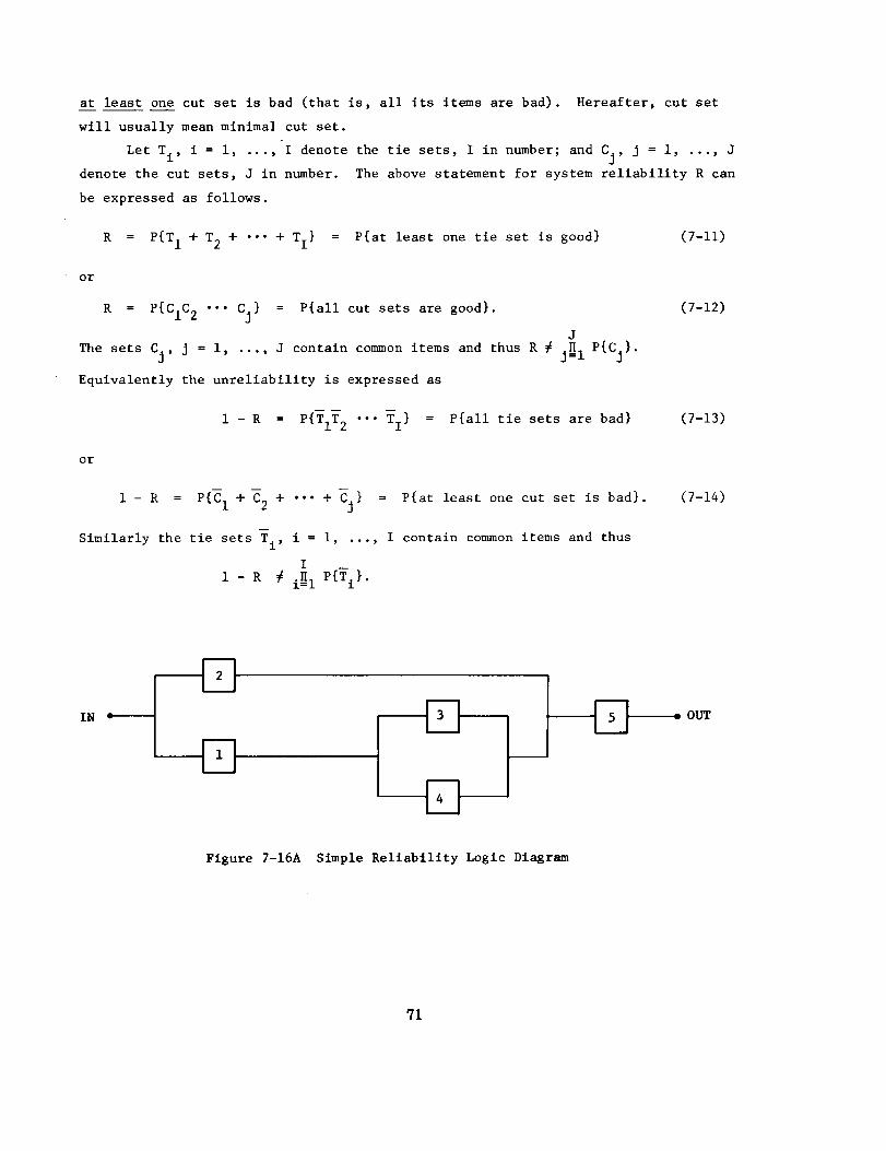
at least one cut set is bad (that is, all its items are bad). Hereafter, cut set
will usually mean minimal cut set.
Let Ti, i = I, ..., I denote the tie sets, I in number; and Cj, j = i, ..., J
denote the cut sets, J in number. The above statement for system reliability R can
be expressed as follows.
or
R = P{T 1 + T 2 + "'" + T I} = P{at least one tie set is good} (7-11)
R = P{CIC 2 "'" Cj} = P{all cut sets are good}.
J
The sets Cj, j = 1 ..... J contain common items and thus R # J_l P{Cj}.
Equivalently the unreliability is expressed as
or
i - R = P{TIT 2 ''- TI } = P{all tie sets are bad}
i - R = P{CI + C2 + "'" + C J} = P{at least one cut set is bad}.
Similarly the tie sets Ti' i = i, ..., I contain common items and thus
I
i - R # iH I P{Ti }.
(7-12)
(7-13)
(7-14)
--F]--
Figure 7-16A Simple Reliability Logic Diagram
: OUT
71
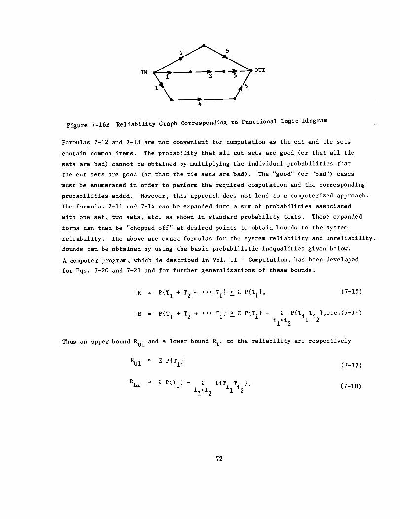
I.L__ j54
Figure 7-16B Reliability Graph Corresponding to Functional Logic Diagram
Formulas 7-12 and 7-13 are not convenient for computation as the cut and tie sets
contain covmnon items. The probability that all cut sets are good (or that all tie
sets are bad) cannot be obtained by multiplying the individual probabilities that
the cut sets are good (or that the tie sets are bad). The "good" (or "bad") cases
must be enumerated in order to perform the required computation and the corresponding
probabilities added. However, this approach does not lend to a computerized approach.
The formulas 7-11 and 7-14 can be expanded into a sum of probabilities associated
with one set, two sets, etc. as shown in standard probability texts. These expanded
forms can then be "chopped off"at desired points to obtain bounds to the system
reliability. The above are exact formulas for the system reliability and unreliability.
Bounds can be obtained by using the basic probabilistic inequalities given below.
A computer program, which is described in Vol. II - Computation, has been developed
for Eqs. 7-20 and 7-21 and for further generalizations of these bounds.
R = P{T 1 + T 2 + "'" T I} ! Z P{TI},(7-15)
R = P{T 1 + T 2 + "'" T I} _ E P{T i} -Z P{TilTi2},etc.(7-16)
il<i 2
Thus an upper bound RUI and a lower bound RLI to the reliability are respectively
_i = Z P{Ti} (7-17)
_i = Z P{Ti} - Z P{TilTi2}. (7-18)il<i 2
72
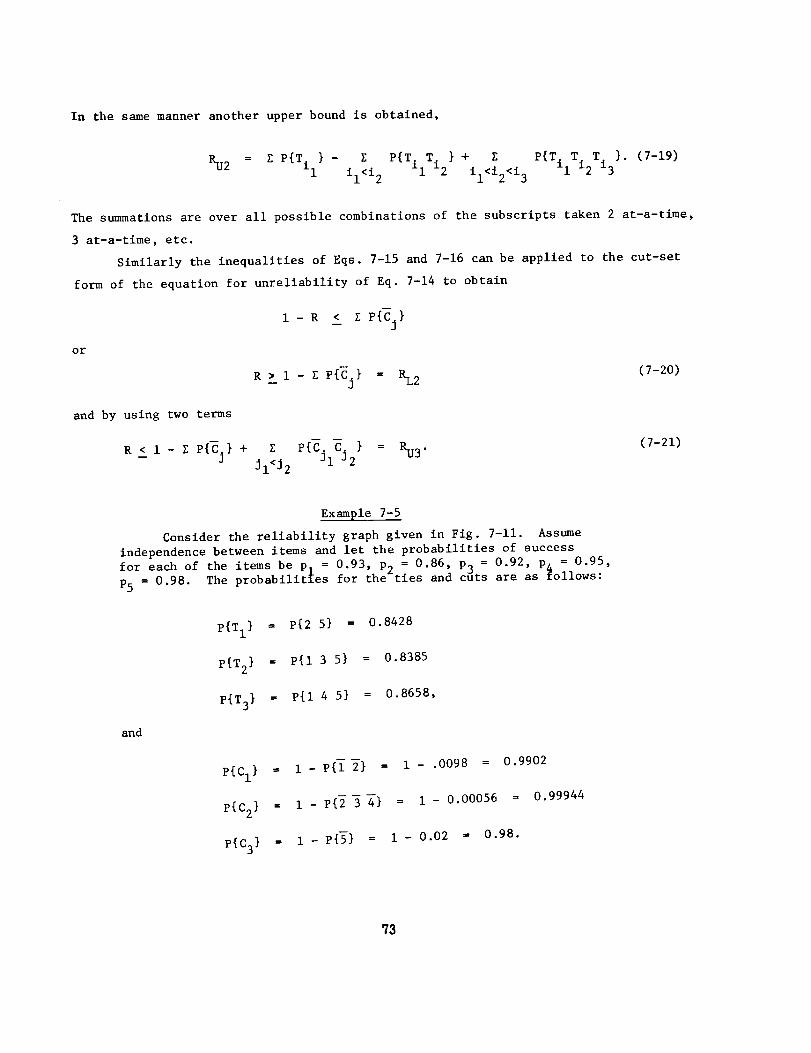
In the same manner another upper bound is obtained,
RU2 = Z P{Til} - Z P{ } + _ }. (7-19)il<i2 TilTi 2 ii<i2<i3 P{TilTi2Ti 3
The summations are over all possible combinatlons of the subscripts taken 2 at-a-time,
3 at-a-time, etc.
Similarly the inequalities of Eqs. 7-15 and 7-16 can be applied to the cut-set
form of the equation for unreliability of Eq. 7-14 to obtain
1 - R <_ T, P{Cj}
or
R _ i - E P{Cj} = _2 (7-20)
and by using two terms
R <_ 1 - 7.. P{"Cj} + y. p{CjlC j } = RU3. (7-21)jl<J2 2
Example 7-5
Consider the reliability graph given in Fig. 7-11. Assume
independence between items and let the probabilities of success
for each of the items be p] = 0.93, p^ = 0.86, P3 = 0.92, p. = 0.95,
P5 = 0.98. The probabilities for theZties and cuts are as _ollows:
and
P{Tl} = P{2 5} = 0.8428
P{T2} = P{I 3 5} = 0.8385
P{T3} = P{I 4 5} = 0.8658,
P{CI} = i - P{Y 2} = i - .0098 = 0.9902
P{C2} = 1 - P{2 3 4} = i - 0.00056 = 0.99944
p{C 3} = 1 - P{5) = 1 - 0.02 = 0.98.
73
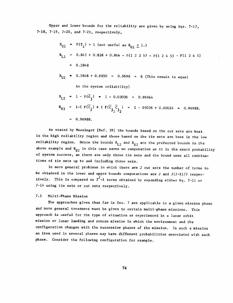
Upper and lower bounds for the reliability are given by using Eqs. 7-17,
7-18, 7-19, 7-20, and 7-21, respectively,
_i = P{Ti} > 1 (not useful as _i <--I.)
_i = 0.843 + 0.838 + 0.866 - P{I 2 3 5} - P{I 2 4 5} - P{I 3 4 5}
= 0.2848
_2 = 0.2848 + 0.6850 = 0.9698 = R (This result is equal
to the system reliability)
_2 = I - P{Cj} = 1 - 0.03036 = 0.96964
u_'3 = 1-E P{Cj} + E P{CJlCJ2 } = i - 03036 + 0.00024 = 0.96988.
= 0.96988.
As stated by Messinger [Ref. 39] the bounds based on the cut sets are best
in the high reliability region and those based on the tie sets are best in the low
reliability region. Hence the bounds RL2 and _3 are the preferred bounds in the
above example and _2 in this case saves no computation as it is the exact probability
of system success, as there are only three tie sets and the bound uses all combina-
tions of tie sets up to and including three sets.
In more general problems in which there are J cut sets the number of terms to
be obtained in the lower and upper bounds computations are J and J(J-l)/2 respec-
tively. This is compared to 2J-i terms obtained by expanding either Eq. 7-11 or
7-14 using tie sets or cut sets respectively.
7.5 Multi-Phase Mission
The approaches given thus far in Sec. 7 are applicable to a given mission phase
and more general treatment must be given to certain multl-phase missions. This
approach is useful for the type of situation as experienced in a lunar orbit
mission or lunar landing and return mission in which the environment and the
configuration changes with the successive phases of the mission. In such a mission
an item used in several phases may have different probabilities associated with each
phase. Consider the following configuration for example.
?4
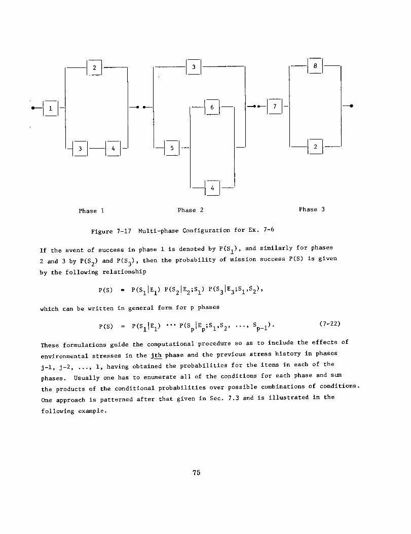
Phase I Phase 2 Phase 3
---e
Figure 7-17 Multi-phase Configuration for Ex. 7-6
If the event of success in phase i is denoted by P(SI) , and similarly for phases
2 and 3 by P(S 2) and P(S3) , then the probability of mission success P(S) is given
by the following relationship
P(S) = P(SIIE I) P(S21E2;S I) P(S31EB;SI,S2),
which can be written in general form for p phases
P(S) = P(SIIE I) "'" P(SplEp;SI,S 2 ..... Sp_l). (7-22)
These formulations guide the computational procedure so as to include the effects of
environmental stresses in the Jth phase and the previous stress history in phases
j-l, j-2 .... , i, having obtained the probabilities for the items in each of the
phases. Usually one has to enumerate all of the conditions for each phase and sum
the products of the conditional probabilities over possible combinations of conditions.
One approach is patterned after that given in Sec. 7.3 and is illustrated in the
following example.
75
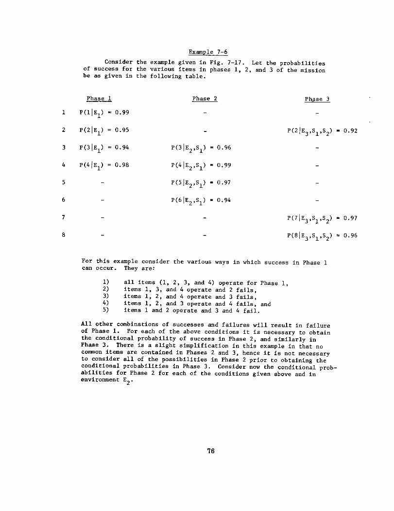
Example 7-6
Consider the example given in Fig. 7-17. Let the probabilities
of success for the various items in phases i, 2, and 3 of the mission
be as given in the following table.
Phase 1
P(IIE l) = 0.99
P(2IE I) = 0.95
P(3[E 1) = 0.94
P(41E 1) = 0.98
Phase 2 Phase 3
- P(21E3,SI,S 2) = 0.92
P(BIE2,SI) = 0.96
P(41E2,S I) = 0.99
P(51E2,S I) = 0.97
P(61E2,SI) = 0.94
- P(71E3,SI,S 2) = 0.97
- P(81E3,SI,S 2) = 0.96
For this example consider the various ways in which success in Phase 1
can occur. They are:
i)2)
3)4)5)
all items (i, 2, 3, and 4) operate for Phase i,
items i, 3, and 4 operate and 2 fails,
items i, 2, and 4 operate and 3 fails,
items i, 2, and 3 operate and 4 fails, and
items 1 and 2 operate and 3 and 4 fail.
All other combinations of successes and failures will result in failure
of Phase i. For each of the above conditions it is necessary to obtain
the conditional probability of success in Phase 2, and similarly in
Phase 3. There is a slight simplification in this example in that no
common items are contained in Phases 2 and 3, hence it is not necessary
to consider all of the possibilities in Phase 2 prior to obtaining the
conditional probabilities in Phase 3. Consider now the conditional prob-
abilities for Phase 2 for each of the conditions given above and in
environment E2 .
76
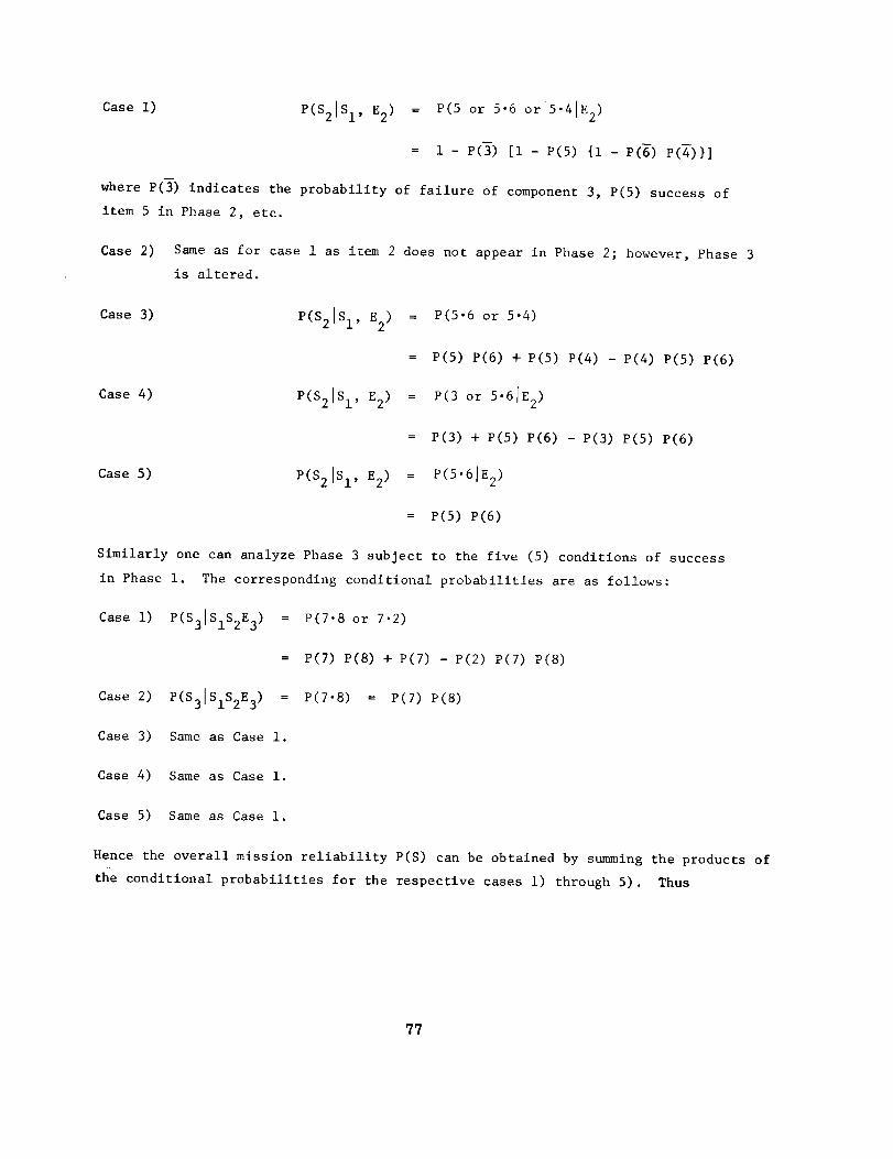
Case i) P(S21SI, E2) = P(5 or 5-6 or 5-41E 2)
= 1 - P(3) [i - P(5) {i - P(6) p(4)}]
where P(3) indicates the probability of failure of component 3, P(5) success of
item 5 in Phase 2, etc.
Case 2) Same as for case 1 as item 2 does not appear in Phase 2; however, Phase 3
is altered.
Case 3) P(S21SI, E2 ) = P(5.6 or 5.4)
= P(5) P(6) + P(5) P(4) - P(4) P(5) P(6)
Case 4) P(S21SI, E2) = P(3 or 5.61E 2)
= P(3) + P(5) P(6) - P(3) P(5) P(6)
Case 5) P(S21SI, E 2) = P(B'6]E 2)
= P(5) P(6)
Similarly one can analyze Phase 3 subject to the five (5) conditions of success
in Phase i. The corresponding conditional probabilities are as follows:
Case i) P(S31SIS2E 3) = P(7.8 or 7.2)
= e(7) P(8) + P(7) -P(2) P(7) P(8)
Case 2) P(S31SIS2E 3) = P(7"8) = e(7) P(8)
Case 3) Same as Case i.
Case 4) Same as Case i.
Case 5) Same as Case i.
Hence the overall mission reliability P(S) can be obtained by summing the products of
the conditional probabilities for the respective cases i) through 5). Thus
?7

P(S) = (0.86639)(.99877)(.9669)
+ (0.04560) (.99877) (.9312)
+ (0.05530)(.96942)(.9669)
+ (0.017681) (.99647) (.9669)
+ (0.001129)(.9118)(.9669)
= 0.949.
The above approach uses the conditional probabilistic approach of Sec. 7.3. The
approach can be rather tedious as it usually would be necessary to list all of the
conditions for each phase and hence the number of different cases would be the
product of the number of conditions in each phase.
Because the above approach can be lengthy and tedious, an approximation to the
mission reliability is possible by use of the method of paths and cuts as described
in Sec. 7.4. In this approach the reliabilities of the components would be taken to
be the reliability up to the end of the last phase in which they are used. If the
probability of failure is assumed to be zero (0) for the phases in which a component
is not used then, the input reliabilities would be equal to the product of the
separate conditional probabilities for each phase.
7.6 N-State Logic Model
The considerations thus far in Sec. 7 have been based on a two-state model for
each item, one failed state and a non-failed or successful state. In this section
we consider a case in which some of the items may be considered as having two or more
failed states, such as opening, shorting, noisy, drift, etc. No additional tools
are needed to solve a problem of this type; however, the analysis does become more
complex. One might need to perform such an analysis in order to make correct
decisions between subsystem configuration. For example, See Ref. 40 which uses a
two-state and a three-state analysis of a particular circuit. As an example consider
a diode-quade with a shorting bar as shown in Fig. 7-18. The circuit fails if two
shorts occur in series (e.g., diodes 1 and 2 or 1 and 4) or if two opens occur in one
end (e.g., diodes 2 and 4 or 1 and 3). Otherwise the system performs successfully.
The probability of a diode opening is denoted by P0 shorting by Ps" Another technique
will be used below to obtain the probability of success or failure. It is certain
that an individual diode will either perform, or short, or open (assuming no other
mode of failure for this analysis). Hence
78
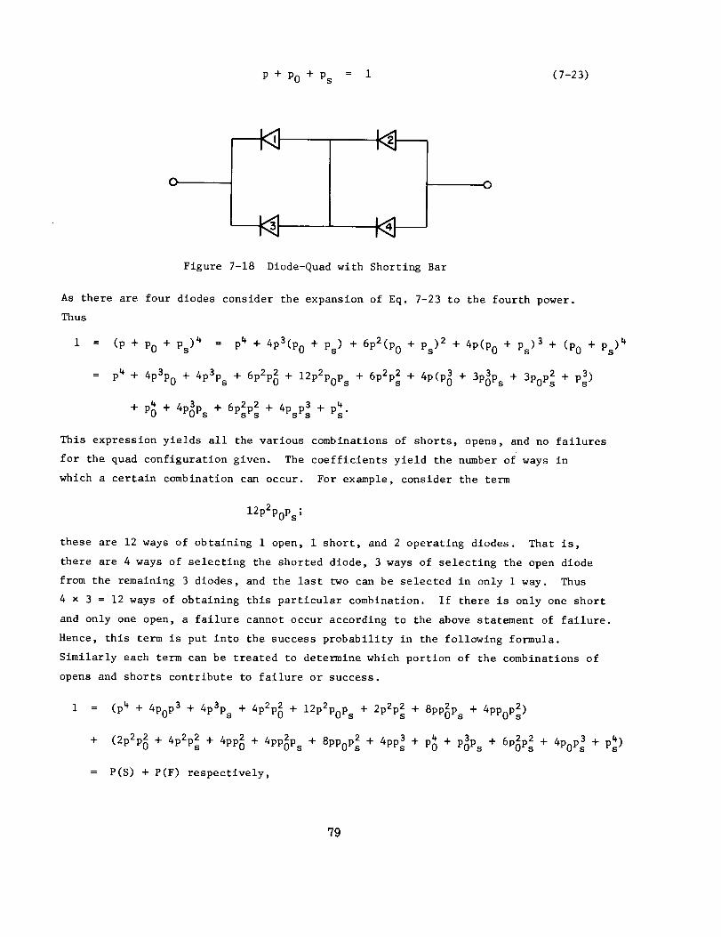
P + P0 + Ps = 1 (7-23)
O O
Figure 7-18 Diode-Quad with Shorting Bar
As there are four diodes consider the expansion of Eq. 7-23 to the fourth power.
Thus
1 = (P + P0 + Ps )_ = P_ + 4p3(P0 + Ps ) + 6p2(po + Ps )2 + 4p(PO + Ps )3 + (P0 + Ps )4
= p4 + 4p3p0 + 4p3ps + 6p2p_ + 12p2P0Ps + 6p2p_ + 4p(p_ + 3p_ps + 3P0P_ + p_)
+ p_ + 4p_p s + 6PsPs2 2 + 4PsP _ + PS"_
This expression yields all the various combinations of shorts, opens, and no failures
for the quad configuration given. The coefficients yield the number of ways in
which a certain combination can occur. For example, consider the term
12p2poPs;
these are 12 ways of obtaining 1 open, i short, and 2 operating diodes. That is,
there are 4 ways of selecting the shorted diode, 3 ways of selecting the open diode
from the remaining 3 diodes, and the last two can be selected in only I way. Thus
4 x 3 = 12 ways of obtaining this particular combination. If there is only one short
and only one open, a failure cannot occur according to the above statement of failure.
Hence, this term is put into the success probability in the following formula.
Similarly each term can be treated to determine which portion of the combinations of
opens and shorts contribute to failure or success.
1 = (p4 + 4POP3 + 4p3ps + 4p2p_ + 12p2poPs + 2p2p_ + 8pp_ps + 4ppop_ )
+ (2p2p_ + 4p2p_ + 4pp_ + 4pp_p s + 8pp0p _ + 4pp_ + p_ + P_Ps + 6POPs22 + 4PoP _ + p_)
= P(S) + P(F) respectively,
79
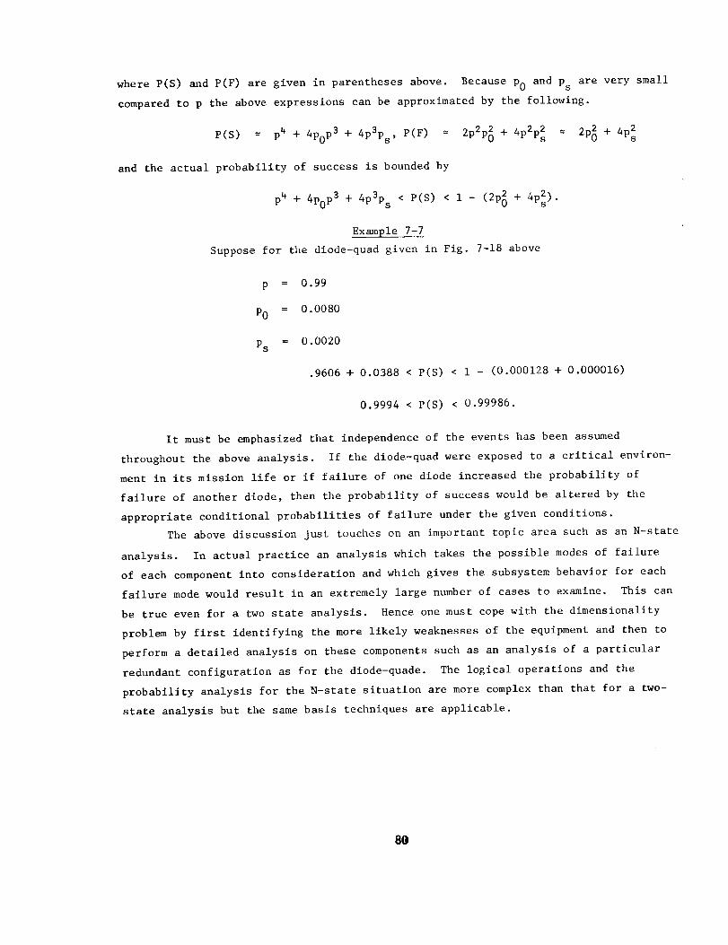
where P(S) and P(F) are given in parentheses above. Because PO and Ps are very small
compared to p the above expressions can be approximated by the following.
P(S) = p4 + 4P0P3 + 4p3Ps ' P(F) _ 2p2p_ + 4p2p_ _ 2p_ + 4p_
and the actual probability of success is bounded by
p_ + 4POP3 + 4p3ps < P(S) < i - (2p_ + 4p_).
Example 7-7
Suppose for the diode_quad given in Fig. 7-18 above
p = 0.99
PO = 0.0080
Ps = 0.0020
.9606 + 0.0388 < P(S) < 1 - (0.000128 + 0.000016)
0.9994 < P(S) < 0.99986.
It must be emphasized that independence of the events has been assumed
throughout the above analysis. If the diode-quad were exposed to a critical environ-
ment in its mission life or if failure of one diode increased the probability of
failure of another diode, then the probability of success would be altered by the
appropriate conditional probabilities of failure under the given conditions.
The above discussion just touches on an important topic area such as an N-state
analysis. In actual practice an analysis which takes the possible modes of failure
of each component into consideration and which gives the subsystem behavior for each
failure mode would result in an extremely large number of cases to examine. This can
be true even for a two state analysis. Hence one must cope with the dimensionality
problem by first identifying the more likely weaknesses of the equipment and then to
perform a detailed analysis on these components such as an analysis of a particular
redundant configuration as for the diode-quade. The logical operations and the
probability analysis for the N-state situation are more complex than that for a two-
state analysis but the same basis techniques are applicable.
80
8. Models Considering Time
In this section the explicit use of time is considered for multi-item problems.
A straightforward approach is to develop a logic model as in Sec. 7 where item suc-
cess and failure probabilities are expressed probabilistically as attributes, and
then to substitute for each attribute the appropriate time measure as described in
Sec. 4.2. This will be discussed first in Sec. 8.1. For some problems the sub-
stitution approach is not applicable, and a more involved convolution approach is
discussed in Sec. 8.2 for these problems. The approaches presented in Secs. 8.1 and
8.2 can be used for the first time to failure of a system where the individual items
can have many possible time to failure distributions such as gamma or log-normal.
However, most often it is assumed that all the items have exponential failure dis-
tributions. Where this assumption is made, the system reliability prediction models
of Sec. 8.1 and 8.2 are applicable regardless of how much operating time has been
accumulated and if it is known that all items in a system are non-failed. Further,
if the exponential failure distribution is assumed for all items, then the methods of
continuous Markov processes and difference equations can be used to develop reliability
models without first developing a logic model. This approach is acknowledged in
Sec. 8.3, along with other approaches which are somewhat specialized. The final
Sec. 8.4 contains the development of a general redundancy equation which is suitable
for general reliability prediction and which also may be used for reliability alloca-
tion decisions.
8.1 Logic Model Substitution
The logic form of reliability prediction models can be readily extended to
explicitly consider time. This is done by simply substituting the applicable
probabilities of success or failure as functions of time, R(t) or F(t), for each
item, into the multi-item logic model. Such a substitution is possible where the
R(t) or F(t) for each item is applicable for the time t of interest, which means that
reliability prediction models for certain systems such as the classical standby
redundancy and the rope models cannot be developed by this method. The following
sections will treat this and considerations other than logic based model substitutions.
In this section several of the logic based models from Sec. 7 will be extended via
examples to consider time explicitly. Those not treated can be readily developed
and are shown in most reliability books and handbooks. Exponential failure time
distributions for items will be used because of its conventional emphasis. Other
distributions can be readily substituted for first-failure time models, but as they
lead to complications if later failures are explicitly considered they are not so
widely used.
81
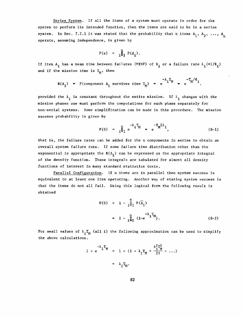
Series System. If all the items of a system must operate in order for the
system to perform its intended function, then the items are said to be in a series
system. In Sec. 7.2.1 it was stated that the probability that n items AI, A2, ..., A n
operate, assuming independence, is given by
n
P(s) = i_ 1 P(Ai).
If item A i has a mean time between failures (MTBF) of 8 i or a failure rate li(=i/Si )
and if the mission time is TM, then
-%iTM -TM/e i
R(A i) = P(component A i survives time T M) = e = e
provided the li is constant throughout the entire mission. If li changes with the
mission phases one must perform the computations for each phase separately for
non-serial systems. Some simplification can be made in this procedure.
success probability is given by
The mission
n -RITM -TMZk i
P(S) i_ 1 e = e , (8-1)
that is, the failure rates can be added for the n components in series to obtain an
overall system failure rate. If some failure time distribution other than the
exponential is appropriate the R(Ai) can be expressed as the appropriate integral
of the density function. These integrals are tabulated for almost all density
functions of interest in many standard statistics texts.
Parallel Configuration. If n items are in parallel then system success is
equivalent to at least one item operating. Another way of stating system success is
that the items do not all fail. Using this logical form the following result is
obtained
n
P(S) = i - i_ I P(A i)
n -AiTM) . (8-2)= 1 - i_ I (l-e
For small values of AiTM (all i) the following approximation can be used to simplify
the above calculations.
_XiTM 2 2kiT_
1 - e = 1 - (i - AiT M + 2--]--- "'')
-- _iTM .
82
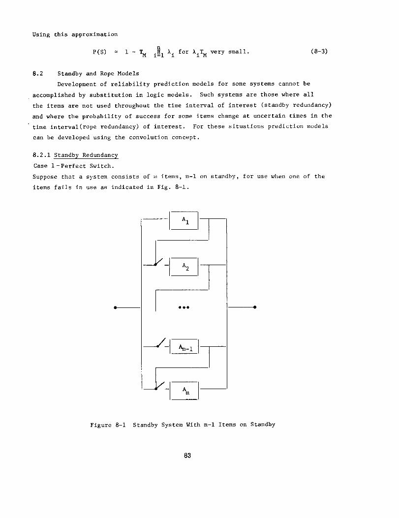
Using this approximation
P(S) =n
i - _ i_1%i for %iTM very small. (8-3)
8.2 Standby and Rope Models
Development of reliability prediction models for some systems cannot be
accomplished by substitution in logic models. Such systems are those where all
the items are not used throughout the time interval of interest (standby redundancy)
and where the probability of success for some items change at uncertain times in the
time interval(rope redundancy) of interest. For these situations prediction models
can be developed using the convolution concept.
8.2.1 Standby Redundancy
Case l-Perfect Switch.
Suppose that a system consists of m items, m-i on standby, for use when one of the
items fails in use as indicated in Fig. 8-1.
---/- Am-1
Figure 8-1 Standby System With m-i Items on Standby
83
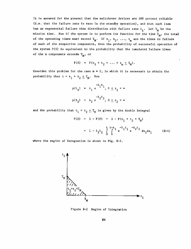
It is assumed for the present that the switchover devices are i00 percent reliable
(i.e. that the failure rate is zero in the standby operation), and that each item
has an exponential failure time distribution with failure rate h i. Let TM be the
mission time. Now if the system is to perform its function for the time TM, the total
of the operating times must exceed TM. If tl, t2, ..., tm are the times to failure
of each of the respective components, then the probability of successful operation of
the system P(S) is equivalent to the probability that the cumulated failure times
of the m components exceeds TM, or
= . . > TM)P(S) P(t I + t 2 + . + tm _ .
Consider this problem for the case m = 2, in which it is necessary to obtain the
probability that t ffitI + t2 _ TM. Now
-%itl
p(t I) = h I e , 0 ! tI <
-A2t 2
P(t2) = _2 e , 0 ! t2 < _
and the probability that tI + t2 _ TM is given by the double integral
P(S) ffi i - P(F) ffi i - P(t I + t2 < TM)
t t_t I -lltl -_2t2= i - Ill2 f e e dt2dt I (8-4)
0 0
where the region of integration is shown in Fig. 8-2.
t2
TM
I+t2<TM
// r//_
TH
_vt I
Figure 8-2 Region of Integration
84
Integration of the equation (8-1) yields
P(S)
-_ITM X Ie + [e -_ITM - e-X2TM],
X2-_ 1If X2 # XI
-XIT M
e [i + AITM ] , If X2 = _i" (8-5)
The above formula can be interpreted as the probability that item 1 survives the
entire mission time plus the probability that item 1 fails in time tI but that
t2 _ TM - tI (the contribution of the second term).
In case the items are all identical and perfect switching exists then the
probability that a system of m components (m-i standby components) survives TM is
given by
P(S)= P(t I + t2 + ... + tm >_ TM)
-_TM( I A2T_-- e + XTM +-_T-+ ... +
Am-ITM m-i
(m-i) !). (8-6)
Note that this formula gives the probability of O, i, 2, ..., m-i failures for a
variable having the Poisson distribution with mean number of failures given by XT M.
Case 2-Imperfect Switch. If imperfect switching were taken into consideration the
second term in the above would have to be multiplied by the probability that the
switch-over occurs, P(sw) say, and hence
-XITM XI -XITM -X2TM]P(S) = e +-- e(sw) [e - e . (8-7)X2-XI
See Ref. 41 for a statement of the above result when several standby components
are allowed. Also see Sec. 8.4 for a more general formula for combinations of
redundancy.
8.2.2 Rope Model
In some physical situations system failure does not occur until all or k out
of n items fail (for example, as strands in a rope), but the failure of some of the
items increases the stresses on the remaining items and thereby decreases their
reliability.
85
Case i: Suppose that the load on a system is constant and that initially n items are
sharing the load. As the elements fail the remaining load is equally shared by the
remaining elements. Thus if the original stress per element is So/n , then the
subsequent stresses increase S0/(n-l) for i failure, S0/(n-2) for two failures, etc.
The increase in stress on each item will usually result in a corresponding increase
in the failure rate for the items as the ratio of the operating stress to the _ated
stress S increases. Let the stress ratio be h as given byr
S0/(n-f) SOh = operating stress = =
rated stress S s Sr r
where f is the number of failures and s(=n-f) is the number of survivors. If the
rated stress is exceeded by S0/s then the system is assumed to fail. Let the maxim,,,
number of failures be n - k, or k be the number of minimum number of items for
Thus for non-failed operation the stress ratio must be less than unity,operation.
i.e.
Solk
h = S < i,r
or
S ffi n-f > k.
Now suppose that the failure rate for an individual item at time t for stress ratio
h is denoted by A(t; h).
In this first case assume that
A(t; h) = Aoh,
that is, _ increases linearly with h, A0 is a constant. The failure rate for the
system AS is given by
A S = sAoh
where s is the number of non-failed or successful items. Now
and thus
S oh =
s Sr
_oSo SO_ 0
_S = s • s S = Sr r
86
which is constant. Ref. 42 treats this case and Ref. 43 has included it as a
special case of finding the reliability of a parallel redundant system when the item
failure rate is X ffiX(h), a general function of the stress ratio.
Thus in this case of constant system failure rate the time to failure of the
system is given by
TS ffi tI + t2 + ... + tf
where f is the number of failures. Now if each t i is assumed to have the exponential
failure time density function, i.e.
p(t i) ffi A S exp(-X S tl),
the distribution of T S is given by the f fold convolution of P(ti),
P(Ts) = P(tl) * P(t2) * ... * p(tf).
For n = 2 items,
P(T s) = P(tl) + p(t 2)
T S
ftl=0
P(t I) P(Ts-tl)dtl
-XsT S
= X_T S e
Similarly for the f fold convolution one obtains
, f f-i exp{_AsTs}
P(Ts) ffi [P(t)]f = AsTs r(f) ' TS > 0. (8-8)
This is the gamma density function with shape parameter f and the same scale parameter
A as for the exponential distribution. See Ref. 44 for further details in the deri-
vation of the distribution. For f = n-k+l yields
P(Ts) ffi r(n-k+l)
lsn-k+l TS n-k exp{-AsT S}
where T S is the time the n-k+is__t_tfailure occurs.
87
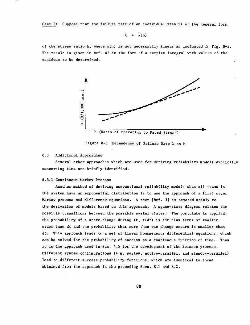
Case 2: Suppose that the failure rate of an individual item is of the general form
= A(h)
of the stress ratio h, where A(h) is not necessarily linear as indicated in Fig. 8-3.
The result is given in Ref. 42 in the form of a complex integral with values of the
residues to be determined.
ooo
v
,<
h (Ratio of Operating to Rated Stress)
Figure 8-3 Dependency of Failure Rate _ on h
w
8.3 Additional Approaches
Several other approaches which are used for deriving reliability models explicitly
concerning time are briefly identified.
8.3.1 Continuous Markov Process
Another method of deriving conventional reliability models when all items in
the system have an exponential distribution is to use the approach of a first order
Markov process and difference equations. A text [Ref. 3] is devoted mainly to
the derivation of models based on this approach• A space-state diagram relates the
possible transitions between the possible system states. The postulate is applied:
the probability of a state change during (t, t+dt) is Adt plus terms of smaller
order than dt and the probability that more than one change occurs is smaller than
dr. This approach leads to a set of linear homogeneous differential equations, which
can be solved for the probability of success as a continuous function of time. Thus
it is the approach used in Sec. 4.5 for the development of the Polsson process•
Different system configurations (e.g. series, active-parallel, and standby-parallel)
lead to different success probability functions, which are identical to those
obtained from the approach in the preceding Secs. 8.1 and 8.2.
88
The Markov process approach can be readily extended to include maintenance,
which is really the advantage of this type of model formulation. Here the state-
space transition diagram is expanded from only failure transitions to include both
failure and repair transitions. The same postulate can be applied to repair as was
applied to failure, resulting in an expanded set of differential equations. These
can be solved for availability formulas. This Markov process formulation is thus
best suited for system level modeling where both maintainability and reliability
are to be explicitly considered, but where the operational profile and the system
are not so complex that an analytical approach becomes unwieldy.
8.3.2 Extreme Value Theory
An approach for obtaining certain prediction equations can be based on concepts
of order statistics when the lifetime distribution of all items are identical and
independent. Here the probability density function is derived for the particular
item which, when it fails, will fail the system. For each of the following systems
this item is:
(i)
(2)
(3)
Series: Shortest lifetime pdf from n series items.
Parallel: Largest lifetime pdf from £ parallel items.
Series Strings in Parallel: Largest lifetime pdf from £
items from the shortest lifetime from n items.
(4) Parallel in Series String: Smallest lifetime pdf from
n items from the largest lifetime from £ items.
As in most practical problems all items do not have identical pdf's, the general
applicability of this approach is restricted.
Example 8-1
If a system consists of n items in series, e.g., linked together
in the form of a chain, the lifetime of the chain cannot be more than
that of the weakest llnk. The life length distribution of the chain
would be that of the shortest llfe length. Ref. 43 treats this
problem. The probability that the shortest llfe is less than t is
given by
Fl(t) = 1 - Prob{llves of all n items are greater than orequal to t}
= 1 - [i - F(t)] n = 1 - Rn(t)
Pl(t) = n[l - F(t)] n-I p(t).
where R(t) = 1 - F(t) is the reliability of a single item
p(t) = lifetime density function of a single item.
89
Suppose that the distribution function for the lifetime of each member of the
chain is Weibull, i.e.
then
and the
BF(t) = i - exp{- ( t-y ) } for x > Y,
8
Fl(t) = I - exp{- n( t-y ) }n
81 B
Pl(t ) -- n_B8( t-y ) exp{_n(t_ ) }.n n
8.3.2 Flowgraphs
Flowgraphs are a graphical method of representing simultaneously a set of
equations which have been applied to electronic and other engineering problems.
They augment a classical mathematical approach. There has been some exploratory
application of flowgraph techniques to the development of reliability prediction
models [Refs. 45 and 46] but this approach is not widely used. An advantage of
a flowgraph approach would be that if one is already skilled in their use for
engineering problems then this may be a ready method for learning about the development
of reliability equations.
8.4 General Redundancy Model
Three of the redundancy models which have been introduced are those for:
(i) all items functioning, i.e. Eq. 8-2 which will be referred
to as items in parallel,
(2) standby redundancy where there is a "perfect" switch, i.e.
Eq. 8-6, which will be referred to as spares, and
(3) standby redundancy where there is a switch, i.e. Eq. 8-7,
which will continue to be referred to as standby redundancy.
Interest is with a general reliability model for parallel arrangements of identical
items of any of these three redundancy approaches where the failure criterion can be
one or more items must work. In addition to reliability prediction this model
can also be used for the general allocation problem concerning optimum selection of
a redundant configuration. This model is an input for a general reliability cost
tradeoff program (RECTA) which is covered in Volume II - Computation.
9O
In this section the following notation is used:
n identical items in parallel,
m identical spares,
r identical items in standby redundancy,
n o number of items that must work,
p switch reliability,
s the number of switches which work,
t the mission time, and
A the failure rate.
The general formulas for the cases in which (a) n o = 1 and (b) no > 1 are
derived separately. Although the first case is a special case of the latter, case
(b), it is useful to derive the simpler case first for a better understanding of the
more general formula.
8.4.1 Reliability of a System for no = 1
In this section the general formula is derived for the situation that only
one item must work.
The probability that s switches work is given by the binomial formula
_) pS(I-P )r-s"
If s switches work then the m spares plus the s items in standby result in m+s items
on "standby", (manual or automatic). Thus the reliability is given by the
formula
[(:) ]R e = s_ 0 pS(l-p)r-s R£(n, m+s; t) ,
where R£(n, m+s; t) is the reliability for a mission of length t given s switches
work, n active items and m spares are available, and hence m+s standby items. The
reliability R£ is given by three cases:
Case i: m+s = 0. In this case the reliability is given simply by the probability
that at least one of the n active items survives time t, that is,
- i e-At nRA 1 - [ - ] .
91
Case 2: m+s = i. In this case the reliability is the probability that the n
active items plus the one (i) standby item survive time t, or
n(;)R_ -- i- j_0
where
(_i) j e-j%t A(j),
1 rt -%t2(l-j)
A(J) = (m+s-l)! j e0
t e-At2(l-j)
0
and for specific values of J we obtain,
A(O) = l-e -At ,
A(1) = At, and
(At2)m+s-I d(At2) , general formula,
d(At 2) for m+s = 1
(j) (J-l)At-l)/(j-l), j = 2, .. n.A -- (e .,
Case 3: m+s = 2, 3, ..., m or m+s is a positive integer larger than i.
If m+s is larger than one (m+s>l) the formula for R£ is the same as the above with
the exception that the A(J) are given by the following formulas which include Case 2
as a special case.
A(0) = i-At
-e
(m+s-l) ![ (At) m+s-I + (re+s-l) (%t) m+s-2
+ ... + (m+s-l)!],
A(1) = (%t)m+S/(m+s)!, and
A(J)e(J-l)%t
(m+s-l) l(j-l) m+s
{ [(j-l)At] m+s-I - (m+s-l) [(j-l)At] m+s-2
+ ... + (-i) m+s-I (m+s-l)!} +(_i) m+s
(j_l)m+s , j = 2, 3 .... , n.
92
Derivation. The derivation of the expression for R£ is given in the following
discussion. First consider the probability that a system of n items in parallel
(all active) will survive time t. Let t(n ) be the longest time of survival for
the n items and hence what is required is the probability that t(n ) > t. The
probability that all n items fail in the interval (0, t) is given by
Fl(t) = P{t(n ) ! t} = Fn(t) (8-9)
and the probability that at least one item survives time t is given by i - Fl(t)
or
P{t(n ) > t} = i - [l-e-%t] n. (8-10)
The probability density function for t(n ) is given by differentiating Fl(t) to yield
Pl(tl) = n[l_e-_tl] n-I e
where tI is substituted for t(n ) for convenience.
It is now desired to find the time to failure distribution for the m+s
"spares" in order to find the total survival time for active and spare items. It
is assumed that the n parallel active items have all failed at time t I and then the
m+s spares will be used one-at-a-time until all have failed. Thus we want the
probability density of the time to failure of these m+s spares with the ass_nption
that one of them is used immediately, at time zero for the spares. The survival
time is the sum of m+s-i times each of which has an exponential failure time density
function. Hence the frequency function for the sum (t2) is the Gamma distribution
-%t 2
P2(t2) = %e (%t2)m+s-i/(m+s-l)f
where t 2 is used to denote the survival time of m+s "spares", automatic and/or manual.
The reliability R_ is given by the probability that the sum of the two survival times
as described above, tI + t 2, is larger than or equal to t, i.e.,
P(t I + t2 _ t).
The probability that the sum is less than t is given by the convolution integral
t
f P2(t2 ) Fl(t-t2)dt 2,
t2=O
where Fl(t-t 2) is obtained by substitution in Eq. 8-9 above.
9S
t -At 2 (At2)m+s-I -A(t-t2)]ni [Ae (m+s-l) l ][l-e dt 20
= I[ e ][j_o (-1)0
j -iX(t-t2)e ] d(Xt 2)
(re+s-l) I
t -At 2 Jlt 2fe e0
(Xt2)m+s-I d(lt2).
Hence, for m+s >__I,
l-R_(n,m+s,t) = P(t I + t2 5_ t) = j_E0 (-i) j A(J),(8-11)
where
A(J)
t -At2(1-J)i le
= (m+s-l) I 0(At2)m+s-I d(At2).
If m+s = O. There is no need for A(J), j = O, I, ..., n, and we use Eq. 8-10
for n items in active parallel.
If m+s = i. For J # i but an integer greater than or equal to zero
t e-%t2(l-J)A(J) = f d(Xt 2)
0
1 [1 - e-At(i-J)],(i-J)
and for J = i
t
A(1) = fd(Xt 2) = At.0
If m+s > i.
A(O) =t -At 2
1 fe(m+s-l) l 0
(It2)m+s-I d(lt2)
= l_e -At [(At) m+s-I + (m+s-l)(At) re+s-2 + ... + (m+s-l) l]/(m+s-l)!
94
1 [t (A t2)m+s_l = (_ t)m+sA(1) (re+s-l) z - d(Xt2) (re+s)'0
A(2)t kt 2
1 fe= (m+s-l)! 0
1A(2) =
(m+s-l) l
(_t2)m+s-I d(_t2)
)_t
e [(At) m+s-I - (m+s-Z) (lt) m+s-2
+ ... + (-I) m+s-I (m+s-l)!] + (-i) m+s
or in general for j _ 2
A(J)e(J-l)%t
(m+s-l) l(J-l) m+s
[[(j-l)At ]m+s-i _ (m+s-l) [(j-l)%t] re+s-2
] (-i) m+s+ ... + (-I) m+s-I (re+s-l)IJ +
(J -i) m+s
Having obtained all Aj, for j = 0, i, ..., n the results are substituted into Eq. 8-11
to obtain
P(t I + t2 ! t),
and then the desired probability is the reliability R£, that is
R£(n,m+s,t) = i - P(t I + t 2 ! t).
This result must be obtained for each possible s and used in the formula for the
reliability of an item,
r[(r) ]Re = s_E0 pS(l-p)r-s R£(n,m+s,t) . (8-12)
95
8.4.2 Reliability of a System for n O _ i
Suppose that nO items must operate in order for a system to properly perform
its function. In the previous derivation nO = i and the distribution of life with
n items in active parallel was given by the maximum life for the n items. In this
case the time to failure is given as the time to failure of the n - n o + it h item.
The probability that the n - n o + it__hitem fails in the interval (t, t+dt) is given
by
n! n-no no-i
P3 (t)dt = (n0-1)l(n-n 0)!'[F(t)] [l-F(t)] p(t)dt,
where the probability density function and distribution function for a single item
are
-%tp(t) = _e ,
-_tF(t) = 1 - e
Thus
-At(no-l+l) _%t]n-noP3(t) = C(n, n0)%e [i - e
nn0(n no)= C(n, no)%e k=EO (-i) k e , (8-13)
where
C(n,no) = nl/[(no-l) 1 (n-no) l].
The distribution function of the time to the n-n 0 + it_hhfailure can be obtained by
integration of P3(t),
! n-n0 (nkn 0 k -lt(k+n0)F3(t ) = C(n, n o) kE_0 (-i) e %dt,
/n-n_ -_ t3 (k+n 0)
n-n0 _ k -J (_l)k+l i [e - I]= C(n, no ) k__E0 (k+n0) ,
where t3 is used to denote the life-length of the n active items. Hence
n-n0 (nkn0) (_i) k+l i -A t3 (k+n0)F3(t3) = C(n_n0 ) kE=O (k+no) e + B(n, no )
96
where
n-n0[(nkno) ]B(n, n O) = C(n, nO) kZ__O (-i) k (k+_0)(8-14)
It is now possible to derive the distribution of t2 + t3 where t2 is the time
to failure of the m+s "spares" and t3 is the time of failure of the n active items
in parallel of which n o must survive. Hence, by convolution of these two distribu-
tions the distribution of t = t2 + t 3 is given by the integral
t.
f P2(t2 ) F3(t - t2)dt 2
t2=O
or
t[ [ no0Cn0)P{t 2 + t 3 <__t} = of Ae-At2 (m_s -- 3! • C(n, n o ) k__E0
-A(t-t2)(k+no)i • e + B(n, n o dt 2.(-i) k+l (k+no)
or
n-n 0 (n_n)I -lt (k+no) 1p{t 2 + t3 < t} = C(n,n o) 7. (-i) k i 0 A(O) - e A(k+n 0)-- k=0 k+no
where A(O) and A(k+n o) are obtained by using the previously derived equations for
A(J) for J = 0 and for J = k+n O.
97
9. Environment and Bound-Crossing Problems
In this section various approaches which have been covered thus far in Parts
II and III are brought together. Mainly the material is concerned with a multl-ltem
system which is to operate in an environment which is known probabillstlcally or
which is comprised of functionally related items. In particular, practical conclu-
sions which can result from the reliability prediction analyses are noted at the ends
of Secs. 9.2 and 9.3. This is the final section of this report concerned with
analytical detail which has immediate practical significance. The following sections
of Part IV mainly present the results of investigations on approaches for bringing
into the analysis more detailed Infomuatlon bearing on the dependence question.
9.1 Environment Described Probabilistically
System reliability logic models such as those developed in Sec. 7 when all
items are independent can be expressed in functional notation as
R = R(R), R = (RI, ..., Rj, ..., Rn)
where R is the reliability for a system and each Rj, j = i, ..., n is the reliability
of a single item. If each Rj is conditional on environment Rjl _ and if the probabil-
ity density of the environments p(_) is known, then the unconditional system reliability
is the expected value,
E(R) = f R(R) p(s)ds. (9-I)
S
This is the extension to multiple item models of the approach noted by Eq. 4-15 for
single items.
Eq. 9-I would be applied to the situation in which each item is used at the
same environment and the envlror_nent is described by a probability density p(s_).
Note that this means that the average reliability of each item cannot be obtained
separately (using Eq. 4-15) and this average reliability substituted into the system
reliability equation R = R(R). That is
f(RII_)(R21 _) p(s)ds # f(Rll _) p(s)d_ f(R21 a) p(s)dsS S S
for the simple case of two serial items. Whether or not using the incorrect separate
approach yields conservative or optimistic results depends on the details of the
particular problem. Some generalized statements of this sort have been developed
98
for certain multi-item stress-strength problems and they will be noted in the follow-
ing section.
The system reliability model R = R(R) may result from any of the configurations
and approaches noted in Sec. 7. The item reliability conditional on environment
could result from testing. An item reliability measure could be of the form of the
various measures of Sec. 4, or it could be based on the bound-crossing concepts
of Sec. 5. For bound-crosslng concepts where the bound is fixed, such as in Sec. 5.2,
the performance attribute y and the environment _ need to be dependent, i.e.,
p(y,s) _ p(y) p(_), in order for the item reliability to be conditional on environ-
ment. Application of the fixed bound would give
Y_
f p(Yl_)dY = RIs •
Y£
This resulting bound-crosslng based reliability measure can then be readily inserted
into Eq. 9-1 as an Ril _ along with other reliability measures for a multi-item system.
An expanded reliability definition which is essentially an elaboration on
Eq. 9-1 has been proposed in Ref. 47 where the orientation was for catastrophic and
drift failure modes for an item in a probabilistlc environment. Eq. 9-1 is thus the
basis of an approach where there is a probabillstic environment if the orientation
is for separate physical items where there is a reliability measure for each item
such as has been the viewpoint throughout Part III, or where the orientation is
for separate failure modes where multiple modes are specifically identified as
in Secs. 4.1 and 4.3, in Ref. 47, and developed in Part IV.
For stress-strength problems where the bound is a distribution such as in
Sec. 5.3 the item reliability is always conditional on the environment (stress).
Extreme value approaches cited in Sec. 8.3.2 for obtaining system reliability
models which explicitly considered time are also applicable for certain multi-item
stress strength problems.
The following section will expand on the multi-item stress-strength problem
using detailed illustrations.
9.2 Stress-Strength Problems
Multi-item stress-strength problems considered here will demonstrate an
application of the more general remarks made in Sec. 9.1. The general problem area
is the extension of the single item stress-strength reliability measure of Sec. 5.3
to a multi-item system. The potential mistake in reliability prediction here is to
99
obtain separately the reliability of each item in a system such as using Eq. 4-15,
and then to substitute this into system logic models as those from Sec. 7. The
correct development of multi-item stress-strength problems is presented in Section
9.2.1 and this is followed with some important practical conclusions in Section
9.2.2.
9.2.1 Prediction Approaches
Two basic approaches are used: (i) the calculation of the conditional proba-
bility that the strength exceeds a given stress and then integrating this result
over the assumed stress distribution, and (2) the derivation of the probability
density function (pdf) for the smallest (or largest) value of strength in a sample
of n items, and then using the joint distribution of this density with that of stress
to obtain the desired probability. Mathematically the first computation can be ex-
pressed as follows:
(I) Obtain the probability that y > so for a single item, i.e.
oo
P(y > so ) = f p(y)dy ,
s o
where so is the fixed stress level, and p(y) is the pdf of strength.
The examples will use uniform distributions and systems with few items,
but the approaches are of course applicable to different distributions
and systems with many items as well as with complex configurations.
(2) Obtain a general expression for the system reliability R in terms
of the item reliabilities, knowing the system configuration. For each
item, substitute the result of (i) into the system reliability model
to obtain a system model as a function of the stress R(s).
(3) Integrate the above reliability model over the stress pdf, p(s),
i.e.
oo
f R(s) p(s)ds ,
s=0
where R(s) is the system reliability as given by (2) above.
The second computation follows the procedure described below:
(i) Obtain the distribution of the smallest strength in the case of a
series logic (or largest strength in the case of parallel logic in which
only one item must operate). For example, the probability that the
smallest item in n selected at random from a distribution function F(y) has
a strength less than y is given by
100
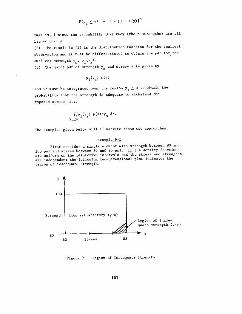
P(Ys ! Y) = i - [i - F(y)] n
that is, i minus the probability that they (the n strengths) are all
larger than y.
(2) The result in (i) is the distribution function for the smallest
observation and it must be differentiated to obtain the pdf for the
smallest strength Ys' PI(Ys )"
(3) The joint pdf of strength Ys and stress s is given by
pl(Ys ) p(s)
and it must be integrated over the region Ys _ s to obtain the
probability that the strength is adequate to withstand the
imposed stress, i.e.
//pl(Ys ) p(s)dy s ds.
YsLs
The examples given below will illustrate these two approaches.
Example 9-1
First consider a single element with strength between 80 and
i00 psi and stress between 60 and 85 psi. If the density functions
are uniform on the respective intervals and the stress and strengths
are independent the following two-dimensional plot indicates the
region of inadequate strength.
i00
Strength
80 --- --J -- J
60 Stress
Item satisfactory (y>s)
! !
85
Region of inade-f quate strength (y<s)
r S
Figure 9.1 Region of Inadequate Strength
101
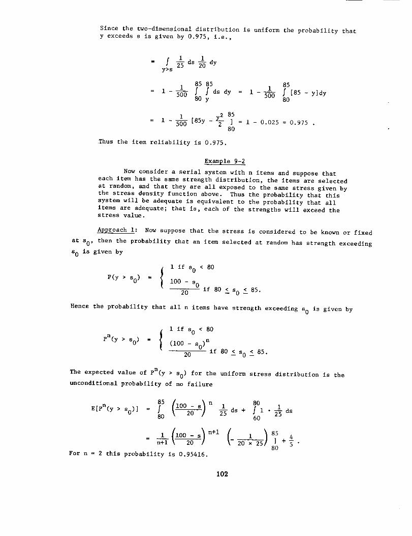
Since the two-dimensional distribution is uniform the probability that
y exceeds s is given by 0.975, i.e.,
_5 1-- f ds _-_ dyy>s
85 85 85
1 f fdsdy -- 1 11 - 50--O - 50---O f [85 - y]dy80 y 80
1 y2 a5500 [85y - 2 ] = i - 0.025 = 0.975 .
80
Thus the item reliability is 0.975.
Example 9-2
Now consider a serial system with n items and suppose that
each item has the same strength distribution, the items are selected
at random, and that they are all exposed to the same stress given by
the stress density function above. Thus the probability that this
system will be adequate is equivalent to the probability that all
items are adequate; that is, each of the strengths will exceed the
stress value.
Approach l: Now suppose that the stress is considered to be known or fixed
at so , then the probability that an item selected at random has strength exceeding
so is given by
I if s o < 80
P(Y • SO) = 1 i00 - so
20 if 80 ! so ! 85.
Hence the probability that all n items have strength exceeding so is given by
i if s o < 80pn(y • SO ) = (i00 - So )n
20 if 80 _ so ! 85.
The expected value of pn(y • So ) for the uniform stress distribution is the
unconditional probability of no failure
( 00)nE[pn(y • s0)] = f _ s. ds + f i • _ ds80 60
(i0020) n+l (_ ) 8]5_ i s i 4
n+l 20 _ 25 +- °80 5
For n-- 2 this probability is 0.95416.
102
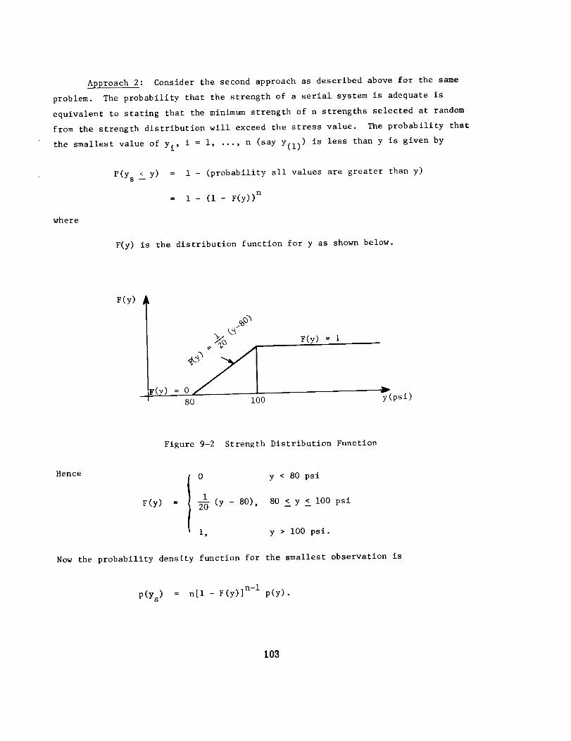
Approach 2: Consider the second approach as described above for the same
problem. The probability that the strength of a serial system is adequate is
equivalent to stating that the minimum strength of n strengths selected at random
from the strength distribution will exceed the stress value. The probability that
the smallest value of Yi' i = i, ..., n (say y(1)) is less than y is given by
where
P(Ys <- y) = 1 - (probability all values are greater than y)
= i - (i - F(y)) n
F(y) is the distribution function for y as shown below.
F(y)
F(y) = 1
! 80 i00 y(psi)
Figure 9-2 Strength Distribution Function
Hence
F(y)
0 y < 80 psi
1
(y - 80), 80 _ y _ i00 psi
i, y > i00 psi.
Now the probability density function for the smallest observation is
p(ys ) = nil - F(y)] n-I p(y).
103
Thus the Joint density function for y and s is
p(ys ) p(s)dy s ds
n-I
= n[l - F(Y)] P(Y) " p(s) dy s ds I
Using the fact that y and s are uniform probability density functions
1 i
P(Y) = 2-O' p(s) = 2-5 "
Hence the probability that Ys ! s (that is, a failure occurs) is given by
i ]n-i i if fn[1 - _ (Ys - 80) 2-O " 2-5 ds dYs
Y!S
851 _ in-i 1
f n[l - _ (Ys 80). 2-_ "80
i
2-_ [85 - Ys]dYs
For n = 2 this reduces to 0.04582 and thus the probability that Yl > s is 0.95416.
Example 9-3
Suppose there are three items in parallel and that at least
one must work (strength exceed stress). Let the strength distribu-
tions he idenuical and uniforms, as given above and let the stress
distribution be the same as above.
Approach i: Using the first approach we obtain the probability that the
strength of a single item exceeds a specified stress so and then integrate this
result over the stress distribution to obtain the unconditional probability. The
probability that for a single element, strength exceeds stress sO is given by
P(y > s0)
1 if so < 80
100 - s0
20 if 80 _ s o _ 85.
The probability that at least one of three exceeds the value so is
1 - P[all three have strength less than sO ]
= 1 - [I - e(y • So)]3,
104
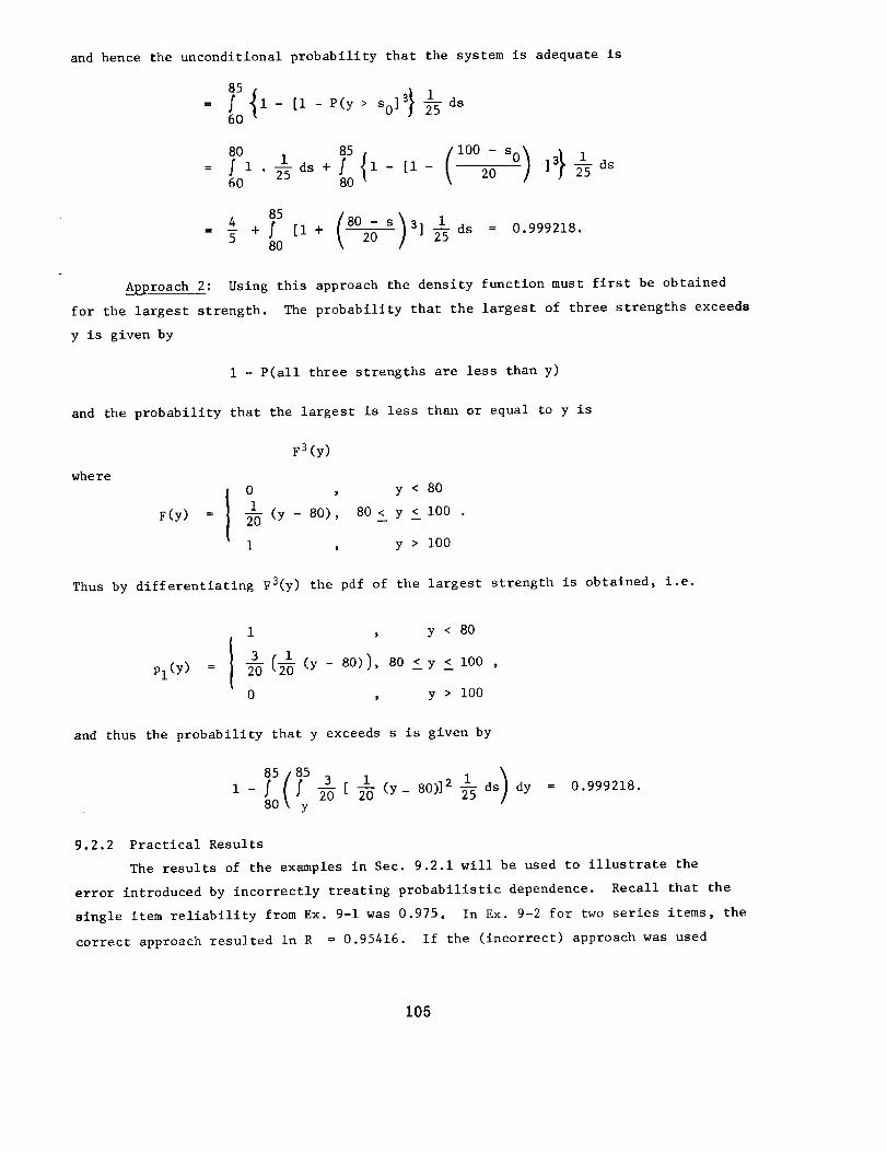
and hence the unconditional probability that the system is adequate is
= . i- [l-P(y> _o] d.60
( 00f 1 ds+f l- [i- ] ds60 80
85
4 f5 +80
Approach 2: Using this approach the density function must first be obtained
for the largest strength. The probability that the largest of three strengths exceeds
y is given by
1 - P(all three strengths are less than y)
and the probability that the largest is less than or equal to y is
where
F(y)
F3(y)
I 20__10 , y< 80: (y - 80), 80 ! Y ! i00 .
1 , y > 100
Thus by differentiating F3(y) the pdf of the largest strength is obtained, i.e.
Pl (y)
1 , y < 80
I+0= ( (y- Bo)), BO!y!lOO ,
0 , y > i00
and thus the probability that y exceeds s is given by
)1 - f _ [ _-_ (y_ 80)]2 ds dy = 0.999218.
80 y
9.2.2 Practical Results
The results of the examples in Sec. 9.2.1 will be used to illustrate the
error introduced by incorrectly treating probabilistic dependence. Recall that the
single item reliability from Ex. 9-1 was 0.975. In Ex. 9-2 for two series items, the
correct approach resulted in R = 0.95416. If the (incorrect) approach was used
105
of treating these as two independent items in series was used then R = 0.9752 = 0.950525.
Thus the incorrect approach resulted in an unwarranted pessimistic reliability for a
series system. Further, in Ex. 9-3 for three parallel items the correct approach
resulted in R = 0.999218. If the incorrect approach of treating these as three
independent items had been used, then R = i - 0.0253 = 0.99925. Thus for a parallel
system the incorrect approach resulted in an unwarranted optimistic reliability.
Although the magnitude of these errors for these examples is not very large, it
should be recognized that only few items were considered. The errors in the above
examples illustrate the results of more extensive analyses in Refs. 48 and 49. These
references show these results with greater elaboration for certain situations where
each item is identical and at the same stress:
(i) Serial System. Obtaining the reliability of each item separately
and then substituting these into a series system model of multiplying
item reliabilities will yleld pessimistic system reliability predictions.
(2) Parallel System. Obtaining the reliability of each item separately
and then substituting this into a logic reliability model will yield
optimistic system reliability predictions.
These results have been shown for situations where the stress-strength distributions
are normal [Ref. 48] and where they are rectangular [Ref. 49]. Some practical
guidelines gleaned from these results and expanded on in these Refs. are:
Serial Systems
(i) Mount items so they experience the same environment, i.e., a compact
unit.
(2) Use consectively manufactured items in the same system, i.e., same
manufacturer and lot.
(3) Select items with similar failure modes.
Parallel Systems
(i) Mount items so they experience different environments, i.e., different
planes and location.
(2) Use items in the same system from different manufacturers and lots.
(3) Select items with different failure modes.
9.3 Functionally Related Variables
A class of multi-ltem bound-crosslng reliability prediction problems are
those where there is no meaningful reliability measure for each item in the system.
In the multl-ltem stress-strength problem of Sec. 9.2 (where in the more general
terminology the item strengths were item performance characteristics and the stress
was the interface characteristic) it was appropriate to have a reliability measure
for each item and a multi-item or system reliability measure. The problem being
106
considered here is a more general one where there is not a performance attribute
for each item, but the performance attributes are only for the system. That is, the
functional relationships between the system performance attributes and the item
and interface characteristics are such that any possible variation in any characteris-
tic can always be compensated for by some possible variation in a different
characteristic. The problem here is to obtain the distribution of the performance
attributes from the distributions of the item and interface characteristics. Then
the bounds are applied to the system performance attributes for the system relia-
- bility prediction. We will not be concerned here in Sec. 9.3 with mixtures of
this more general problem with those of Secs. 9.1 and 9.2. The reader interested
in such complexities is referred to Part IV. Some practical problems which have
been widely treated in reliability analysis are those for performance variation
analysis of electronic circuits and of systems in general [Ref. 7].
The basic procedure for reliability prediction of functionally related
variables is as follows:
(i) Select the performance attributes of interest. These most often
are functional outputs.
(2) Develop the deterministic mathematical models at nominal conditions
relating the performance attributes to item and interface characteristics.
(3) Estimate the variability of the item and interface characteristics.
For electronic parts these typically reflect the initial (manufacturing)
variations, aging effects, and the influence of environmental inputs.
(4) Compute the following:
a. The expected variability of and possibly the correlation
between the performance attributes.
b. Identify sources of performance attributes variability.
Possible sources include contributions from the linear, non-
linear, and interaction behavior of the deterministic models,
and from variations and correlation between the independent
variables.
c. Predict the probability of successful performance by
assigning limits to the expected performance attribute
variations.
The more practical benefits are using the results of (4) for identifying designs
which are susceptible to failure, and for providing redesign guidance. They are
also useful for comparing alternate design approaches, and for aiding the assignment
of specification limits. Normally the prediction of the probability of acceptable
performance that can be obtained from a performance variations analysis is not highly
107
precise because the approach is an approximate one, but more so because of the lack
of precision in the data on part and interface characteristic behavior.
A solution to the problem in closed form is almost never possible, but
mainly provides a better understanding of what an approximate approach is attempt-
ing. (See the discussion in Section ii concerning Mode 2 for identification of
an approach in closed form.) What is usually done in practice is use an approximate
approach such as the method of moments (sometimes called the propagation of errors).
Other approaches are identified in Ref. 7. The method of moments approach is
presented below as an illustration.
9.3.1 Method of Moments
In the moments approach the functional relationship is expanded in a Taylor
series. Higher order terms may be used, although most applications only use the
linear terms. Measures of location and variability of the item and interface
characteristics, which are the independent variables, are described by means and
central moments. The degree of association which might exist between two independent
variables is described by the correlation coefficient. The mean and central moments
of the dependent variables are obtained from the application of expected value
theory, which gives the mean and central moments of the dependent variable as
functions of terms obtained from the Taylor series expansion and the mean and central
moments of the independent variables. The distribution of the performance variables
is then obtained by either assuming a distribution, or by fitting a distribution by
the method of equating moments, for example. Correlation between the various
performance attributes can also be obtained by this approach, but this is not
usually noted or developed in reliability applicatons of this technique.
For simpler problems, requiring the use of only first order terms, it is
possible to use this technique without a computer. Conversion of the functional
model to a Taylor series yields sensitivity and possible interaction terms which
readily provide information on variability sources. When the problem becomes more
complex, as an involved functional relationship and high order moments, a computer
is required. Advantages of this approach are simplicity for easier problems, and
resultant information on sources of variability.
Mathematically the method of moments for a single performance attribute is
as follows:
If the relationship
y = Y(Xl, x 2 ..... xn)
can be approximated by a linear function
108
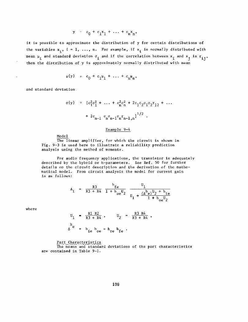
Y cO + ClX I + +__ ... CnX n
it is possible to approximate the distribution of y for certain distributions of
the variables x., i = i, ..., n. For example, if x. is normally distributed with1 1
mean _i and standard deviation oi and if the correlation between xol and xj is rij ,
then the distribution of y is approximately normally distributed with mean
_{y} = co + Cl_ 1 + ... +CnB n,
and standard deviation
where
o{y} _ 2 2 e2_2[ClCl + "'" + n n + 2ClC2Ci°2r12 + "'"
+ 2Cn_ I CnOn_i°nrn_l,n ]I/2
Example 9-4
Model
The linear amplifier, for which the circuit is shown in
Fig. 9-3 is used here to illustrate a reliability prediction
analysis using the method of moments.
For audio frequency applications, the transistor is adequately
described by the hybrid or h-parameters. See Ref. 50 for further
details on the circuit description and the derivation of the mathe-
matical model. From circuit analysis the model for current gain
is as follows:
A°1
R3 hfe U1
R3 + R4 1 + hoeU 2
U 1 +
(Ahe)U2 + hie
I + hoeU 2
RI R2 R3 R4
UI = R3 + R4 ' U2 = R3 + R4 '
he
A= hie h - hoe re hfe
Part Characteristics
The means and standard deviations of the part characteristicsare contained in Table 9-1.
109
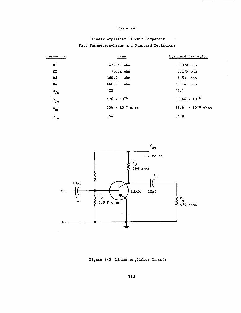
Table 9-1
Linear Amplifier Circuit Component
Part Parameters-Means and Standard Deviations
Parameter
RI
R2
R3
R4
hfe
hre
hoe
hie
Me an
47.05K ohm
7.03K ohm
380.9 ohm
468,7 ohm
102
576 x 10 -6
556 x 10 -6 mhos
254
Standard Deviation
0.97K ohm
0.17K ohm
8.54 ohm
ii. 14 ohm
ii. 1
0.46 x 10 -6
68.6 x 10 -6 mhos
24.9
lOuf
I,(C 1
6.8 K ohms
VCC
Z
-12 volts
R 3
390 ohms
2N526
Li
C 2
I(10_f
m
R 4
470 ohms
Figure 9-3 Linear Amplifier Circuit
110
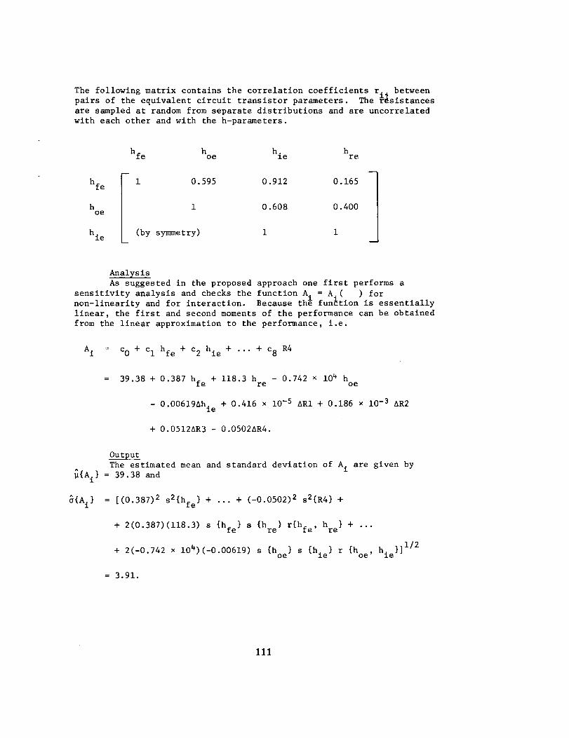
The following matrix contains the correlation coefficients r i. betweenpairs of the equivalent circuit transistor parameters. The r_sistances
are sampled at random from separate distributions and are uncorrelated
with each other and with the h-parameters.
hfe
hoe
hie
hfe
1
h hoe hie re
0.595 0.912 0.165
i 0.608 0.400
(by symmetry) i i
Analysis
As suggested in the proposed approach one first performs a
sensitivity analysis and checks the function A i = A.( ) forlnon-linearlty and for interaction. Because the function is essentially
linear, the first and second moments of the performance can be obtained
from the linear approximation to the performance, i.e.
A i = co + cI hfe + c2 hie + ... + c8 R4
= 39.38 + 0.387 hfe + 118.3 hre - 0.742 × 10⁴ hoe
- 0.00619&hie + 0.416 × 10 -5 &RI + 0.186 × i0 -S AR2
+ 0.0512AR3 - 0.0502AR4.
Outup_!
The estimated mean and standard deviation of A i are given by
_{A i} = 39.38 and
o{A i} = [(0.387) 2 s2{hfe} + ... + (-0.0502) 2 s2{R4} +
+ 2(0.387)(118.3) s {hfe} s {hre} r{hfe, hre} + ...
+ 2(-0.742 x i0_)(-0.00619) s {h } s {hie} r {hoe, hie}] I/2oe
= 3.91.
III
Remark i. A reliability prediction is obtained by assigning a desired limit and then
by obtaining a numerical value from any normal distribution table.
Remark 2. If the function could not be approximated by a linear function higher order
moments and/or distributions of the part characteristics would be required.
Remark 3. The standard deviations and means used in the above analysis were
inherent variations in the part characteristics. Variation as a result of operation
environment, inputs, stresses, loads, and/or aging were not included. The analysis
would be the same except that the total standard deviations would be larger than the
above. In addition, correlations between the behavior of the parts characteristics
may be introduced as a result of changes in a third variable, such as temperature,
affecting two or more part characteristics.
112
Part IV. Refinements of Prediction Models
Some material concerning the structuring of reliability prediction models is
presented in this part. The intent here is to provide insight somewhat beyond the
current conventional practices. On occasion a hue and cry is raised as to whether
or not current conventional practices are appropriate. Anyone who has performed
reliability predictions and who has given serious consideration to the appropriate-
ness of these predictions has likewise on occasion felt a bit uncomfortable. Yet, to
many persons it is not obvious how to go beyond conventional practices.
The material presented in Part IV is directed toward those who are concerned
with the development of reliability prediction models. A frame of reference is
presented which will fit together details of certain reliability prediction problems.
There are strong limitations on the extent to which these notions can be applied to
real problems, with the main limitation being data.
To develop an approach to structuring certain features of reliability predic-
tion models which reflects more detail is a stumbling point. The difficulties may
eventually turn out to be elementary in hindsight, but documentation providing
guidance on the type of problem considered in the following sections is rare.
Remarks will be made freely in the hope that some may be of help in overcoming these
difficulties. The following questions introduce some possible stumbling points and
questions of interest.
(i) What is to be done if the conventional assumption of probabilistic
independence is not made? What are sources of dependence and how are
they reflected in structuring the problem?
(2) What are the features of a failure mode? How are variables treated
which are probabilistic but which do not have values that always
cause a failure?
(3) What is the pertinence of the typical engineering deterministic
equations used for obtaining performance and stress.
(4) What is the relationship between degradation or catastrophic
failure at the source (point of repair) and the manner in which system
performance will be affected?
(5) How are the above considerations brought together?
(6) What are the implications of replies to these questions on real-
world reliability predictions and on other reliability analyses?
113
Two examples are considered in some detail in Secs. i0 and Ii to intrdduce the
notation and to formulate or structure the reliability prediction problem. Sec. 10
is a discussion of an example which is intended to illustrate features concerning
catastrophic and degradation failures. A number of related problems are simultaneously
treated in a different example presented in Sec. ii. The purpose is to structure
the problems and not to obtain numerical solutions. Next in Sec. 12 the points made
in Secs. I0 and ii are expressed in general notation which results in detailed
reliability prediction models. The above questions are replied to individually in
Sec. 13 based on the contents of Secs. i0, ii, and 12, serving as concluding remarks
for Part IV.
This material is somewhat related to earlier efforts at RTI supported by
NASA ORQA [Ref. 47].
114
i0. Catastrophic and Degradation Failures
There are two broad classes of failure modes which are popularly cited; these
are a catastrophic failure and a degradation (or drift) failure. A degradation
failure is an unsatisfactory level of a performance attribute, and a catastrophic
failure is an abrupt change in a performance attribute, usually culminating in no
meaningful measure of the performance attribute.
The question here is, "Is there a unique relationship between the classification
of system failure into catastrophic or degradation and a similar classification of
the source (point of repair) of system failure?" The answer will be developed by
considering some failures associated with an electronic transmitter.
Catastrophic failure at the source:
(i) A part within a system opens or shorts. The result could be an irmnediate
catastrophic failure of an output performance attribute, thus a catastrophic failure;
or, the result could be a degradation failure of an output performance attribute.
For example, the heater winding of a temperature control oven opens and the carrier
frequency of a transmitter drifts. The oven winding open is an illustration where
the system would not immediately fail, but rather results in an increased probability
or later system failure.
(2) An input such as a supply voltage is completely lost. This results in
the complete loss of all performance attributes.
Degradation failure (or conditions) at the source:
(i) An output performance attribute crosses a bound and is considered to
have failed. Here there is some value of the performance attribute present, but it
is outside of the desired range. This type of failure may have no single cause, as
there may be several different parts which could be changed in order to correct the
failure. There may be several items considered as failures according to the bounds
on the performance characteristic in each part's specification, or there may be no
part considered as having failed according to these criteria. Here there would be a
functional relationship between the output performance attribute and the characteristics
of the parts.
(2) An internal performance attribute crosses a bound, which causes an output
performance attribute to fail catastrophically. An example is an oscillator ceasing
tO oscillate because of part characteristic value changes, with the result that an
output performance attribute fails catastrophically. This type of failure is similar
to the above as it may have no single cause.
The above examples illustrate that there is no unique correspondence between
catastrophic and degradation failure modes at the detailed level (source) to that
at the system output performance attribute level. That is, a catastrophic failure
115
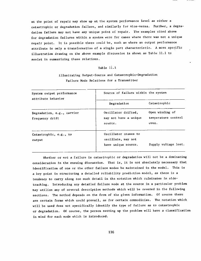
at the point of repair may show up at the system performance level as either a
catastrophic or degradation failure, and similarly for vice-versa. Further, a degra-
dation failure may not have any unique point of repair. The examples cited above
for degradation failures within a system were for cases where there was not a unique
repair point. It is possible there could be, such as where an output performance
attribute is only a transformation of a single part characteristic. A more specific
illustration drawing on the above example discussion is shown as Table ii.i to
assist in summarizing these relations.
Table li.l
Illustrating Output-Source and Catastrophic-Degradation
Failure Mode Relations for a Transmitter
System output performance
attribute behavior
Degradation, e.g., carrier
frequency drift
Catastrophic, e.g., no
output
Source of failure within the system
Degradation Catastrophic
Oscillator drifted,
may not have a unique
source.
Open winding of
temperature control
oven.
Oscillator ceases to
oscillate, may not
have unique source. Supply voltage lost.
Whether or not a failure is catastrophic or degradation will not be a dominating
consideration in the ensuing discussion. That is, it is not absolutely necessary that
identification of one or the other failure modes be maintained in the model. This is
a key point in structuring a detailed reliability prediction model, as there is a
tendency to carry along too much detail in the notation which culminates in side-
tracking. Introducing any detailed failure mode at the source in a particular problem
may utilize any of several description methods which will be covered in the following
sections. The method depends on the form of the given information. Of course there
are certain forms which could prevail, as for certain commodities. The notation which
will be used does not specifically identify the type of failure as to catastrophic
or degradation. Of course, the person setting up the problem will have a classification
in mind for each mode which is introduced.
116
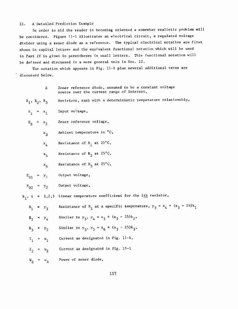
ii. A Detailed Prediction Example
In order to aid the reader in becoming oriented a somewhat realistic problem will
be considered. Figure ii-i illustrates an electrical circuit, a regulated voltage
divider using a zener diode as a reference. The typical electrical notation are first
shown in capital letters and the equivalent functional notation which will be used
in Part IV is given in parentheses in small letters. This functional notation will
be defined and discussed in a more general vein in Sec. 12.
The notation which appears in Fig. ii-i plus several additional terms are
discussed below.
Z Zener reference diode, assumed to be a constant voltage
source over the current range of interest,
Resistors, each with a deterministic temperature relationship,
Input voltage,
Zener reference voltage,
Ambient temperature in =C,
Resistance of R I at 25°C,
Resistance of R 2 at 25°C,
Resistance of R 3 at 25°C,
Output voltage,
= Y2 Output voltage,
= 1,2,3 Linear temperature coefficient for the ith resistor,
= Y3 Resistance of RI at a specific temperature, Y3 = x4 + (x3 - 25)ki
= Y4 Similar to Y3' Y4 = x5 + (x3 - 25)k2'
Similar to Y3' Y5 = x6 + (x3 - 25)k3'
Current as designated in Fig. ii-i,
R I , R 2 , R 3
Eo = x Ii
EZ = x 2
x3
x4
x 5
x 6
E01 = Yl
E02
ki, i
R 1
R 2
R3 = Y5
I I = u I
12 = u 2
W Z = u 3
Current as designated in Fig. ii-i
Power of zener diode,
117
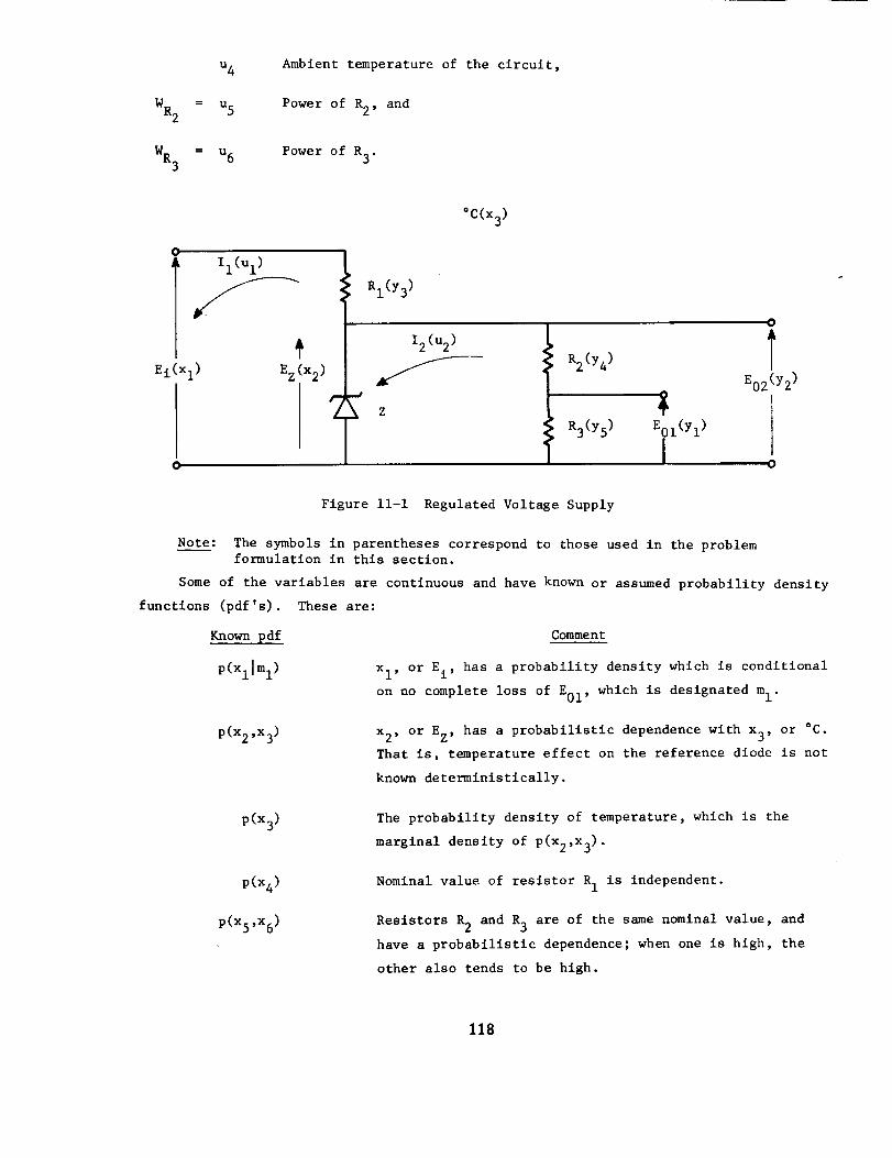
u4
WR2 = u5
WR3 = u6
Ambient temperature of the circuit,
Power of R2, and
Power of R3.
O
I ll(Ul)
gi(xl ) Ez (x 2)
L
0
°C(x3)
RI(Y 3)
O
I2(u2) I
Z/_ R2(Y4)-- E02(Y2)
R3(Ys) _ I(yl) I
O
Figure ii-i Regulated Voltage Supply
Note: The symbols in parentheses correspond to those used in the problemformulation in this section.
Some of the variables are continuous and have known or assumed probability density
functions (pdf's).
Known pdf
P(Xllm I)
These are:
Comment
Xl, or El, has a probability density which is conditional
on no complete loss of EOI, which is designated m I.
P (x2 ,x 3) x2, or EZ, has a probabilistlc dependence with x3, or =C.
That is, temperature effect on the reference diode is not
known deterministically.
P(x 3) The probability density of temperature, which is the
marginal density of P(X2,X3).
P(x 4) Nominal value of resistor R I is independent.
P(Xs,X 6) Resistors R 2 and R 3 are of the same nominal value, and
have a probabilistic dependence; when one is high, the
other also tends to be high.
118
The circuit is designated as having seven different failure modes:
j = 1
j = 2
j = 3
j = 4
j = 5
J = 6
J = 7
m.3
Complete loss of El,
Drift of EOI (or yl ) outside of an acceptable interval
of values r
YI'
Drift of E02 (or y2 ) outside of an acceptable interval
of values FY2'
Catastrophic failure of Z,
Catastrophic failure of RI,
Catastrophic failure of R 2,
Catastrohpic failure of R3, and
Event that the jth failure mode does not occur.
Catastrophic failures noted above are those which might occur as influenced by
the internal stresses. It is known that each item is not initially catastrophically
failed. Additional known information concerns each catastrophic failure mode, m 4
though m 7. Relationships between the probability that these failure modes will not
occur and appropriate environments are known; thus P(mjl...environment(s)...) = __m_('''en-
vironment(s)...) are available for m 4 through m 7. Note that conventional graphs for
failure rate versus stresses such as those found in MIL-HDBK-217A [Ref. 27] could
provide this type of relationship.
The functional notation for deterministic relations will be such as Y3 =
y_(x3,x4) , P(m41u3,u 4) = m4(u3,u 4), and uI = Ul(Xl,X2,X3,X4).
The question is how to structure the problem for the probability that none of
these failure modes occur, where no assumption of independence is made involving the
features noted above. Each of the failure modes will be treated separately and then
they are brought together into a composite model.
Mode m I
Mode reliability P(m I) is some known value between 0 and i.
119
Mode m 2
Electrical equations are conventional engineering deterministic ones and are
used for obtaining the performance attribute E01 (or yl ), i.e.
Y5X2
E01 = Yl Y4 + Y5- Yl(X2,X3,X5,X6)
where Y4 and Y5 are known functions of x3, x5, and x 6. The zener reference voltage
x 2 is dependent on x 3 the ambient temperature and the joint pdf P(X2,X 3) has been
obtained. The mode reliability P(m 2) is the probability that Yl falls within the
interval of acceptable values, r . If p(yl ) denotes the pdf of YI' thenYl
P(m2) = f P(Yl)dY •rYl
However a difficult problem is implied by the above integration, that of obtaining
p(yl ) using the functional relationship given above.
In some few problems a transformation can be defined relating the new variable
Yl to the original variables x2, x4, x5, x 6 and the distribution of the new variable
obtained from that of the original variables by means of the Jacobian of the transforma-
tion. (See Ref. 51 for a description of the method.)
Usually the above approach is tedious or the integral cannot be obtained in a
closed form. In such cases, which is the usual situation, one has to use some other
approach. Often the method of moments is used in which Yl is expanded in a Taylor
Series using the first order terms (higher order terms may be used but seldom are) and
obtaining the moments of Yl (first and second order) in terms of the moments of
x 2, x3, x5, and x 6. Hence the distribution of Yl is approximated by the method of
moments.
Another procedure is to evaluate the integral
P(m2) = /r
Yl
P(X2,X 3) P(Xs,x6)dx2dx3dxsdx 6
where r determines a region of integration of x2, x3, x5, and x 6. This is still
difficu[_ but some approximations may be possible and a Monte Carlo simulation could
be used to obtain the estimate. However the latter approach would require a very
large number of trials if P(m2) is near 1 and a high precision of the estimate is
desired.
120
Although each of the above procedures is suitable for estimating the reliability
of this mode, the latter one will be required for bringing together all modes for a
single circuit reliability model. This will be treated later.
Mode m 3
The performance attribute E02 (or y2 ) is known:
E02 = EZ' Y2 = x2"
Mode reliability is defined to be the probability that Y2 (or x2) falls within PY2'
i.e.
P(m3) = f f P(X2,x3)dx2dx 3"
x 3 rY2
Mode m 4
Electrical equations needed here are the conventional ones for the power stress
W z •
W Z = u 3 = EZ(I 1 - 12 ) = x2(u I - u 2)
where
E i - EZ x I - x 2
Ii = Ul - R1 Y3
E Z x 2
I2 = u2 = R2 + R3 = Y4 + Y5
The mode reliability P(m 4) is defined as the probability of no catastrophic failure
of the zener reference diode Z. The relationship of P!(m4) to fixed levels of the
stresses of temperature °C and power W Z is known:
P(m4[Wz,°C) = P(m4[u3,u4) = m4(u3,u4).
The power u 3 is a function of x (all the x's) denoted by u 3 = u3(x). The ambient
temperature u4 is known, °C = x 3 = u4. Now x has a joint pdf denoted by p(x).
Hence the mode reliability is the expected value
121
E[P(m41u3,u4) ] _ f m4[x3,u4(_)] p(x)dx.X
The reason for obtaining the expected value of the probability of no failure given
the stress is the fact that some or all of the x's are probabilistic variables having
pdf's. If the failure occurred when the stress exceeded a particular value then the
probability would be obtained in a manner similar to that of m 2 and m 3.
Mode m 5
No electrical equations are used as the relation of P(m 5) contains only a single
stress, temperature, °C:
P(m51°C) = P(m51u4) = m5(u4) where u 4 = x 3.
Mode reliability is the expected value
E[P(m51u4) ] = / m5(x 3) P(x3)dx 3-
x 3
Mode m 6
Electrical equations are for the power stress WR2.
WR2 = u 5 = I_ R 2 = u_ Y4
where u2 is noted in m 4. Mode reliability is similar to m4:
P(m6 I°C,WR2) = e(m61u4,u 5) = m6(u4,u5)
where u 4 = x 3 and u5 = Us(X2,X3,X5,X6) = u5(x'), say where _' = x2,x3,Xs,X 6.
E[P(m61u4,u5)] = / m6[x3,u5(x')] p(x')dx_'X v
Mode m 7
The development here is similar to m6, where Y4 for m 6 become Y5 for m 7.
m 7 reliability in functional notation is identical to that for m 6.
The
122
Composite Reliability
The reliability of the circuit is the probability that none of the failure modes
occur;
R = P(mlm 2 ... m 7)
Although this probability can be expressed as the product of conditional reliabilities,
R = P(m I) P(m21ml)...P(m71ml .... , m6),
this does not aid in the evaluation of the reliability in this example due to the
commonality of the variables x to the various modes. Thus the mode reliabilities
which were formulated individually in the previous discussion cannot be multiplied
together to obtain the overall reliability. The circuit reliability is obtained by
the evaluation of a multiple integral which simultaneously considers the probabilities
of non-failure of the seven modes. Thus
R = P(m I) f
{Xl,X 4 }
f
x'CFyll
and I
x 'CFy2_
m4(_) m5(x 3) m6(_') m7(x') P(Xlml)d_
where all terms are as developed in the preceding discussion. The region of integra-
tion is a restricted one for only certain values of x' that is those contained in
F and F , is there a success. In words the reliability of the circuit is a multiple
i_egral Y2over the acceptable regions of the variables defined by bounds. The integral
contains the product of the conditional probabilities of non-failure of those modes,
conditioned on the environment distributions.
The above reliability expression is rather formidable, indicating that considera-
tion of dependence resulting from correlation between variables and from the effect
of the same basic variables on more than one mode reliability yields a complex
relationship.
A numerical integration would be tedious and require a computerized solution.
It would not seem possible to provide a single computer program to treat a very wide
class of these problems although specific subroutines are available to perform
numerical integrations. Thus one must use an approximate numerical solution. The
simplest approach would seem to be a Monte Carlo simulation. Numerical computation is
discussed later in Sec. 12.2.
123
12. General Model Development
The features which were contained in the example problem of Sec. ii are
brought together and are expressed in general notation. This notation explicitly
allows much detail (known or starting information), but only part of this detail
would be expected in a specific problem. Keep in mind that the example of Sec. Ii
was an illustration of this generalization.
In Sec. 12.1 a prediction model is developed for the series situation where
occurrence of any failure mode will imply system failure. Numerical solution
approaches are briefly covered in Sec. 12.2 for the series situation model. Next,
Sec. 12.3.1 briefly comments on extending the series model to include the explicit
treatment of time. The final Sec. 12.3.2 comments on the extension of the series
situation model to a parallel situation where some failure modes can occur but the
system remains unfailed.
12.1 Series Situation Model
A detailed reliability prediction model is developed for the situation where
the occurrence of any failure mode results in system failure. This will be referred
to as the series situation model. However, the reader is cautioned not to expect
that the final composite model will literally be a product of individual probabilities
of non-failure of each mode. Explicit consideration of mode dependencies results in
the final composite model being of a different form than a product.
12.1.1 Notation
Much of the material in Secs. I0 and Ii pertains to the selection of notation.
Seeing how to structure the detailed reliability prediction problem considered here
is aided by an approach which leans toward using common notation for mathematically
similar descriptions rather than using different symbols for the different physical
features having common mathematical descriptions.
As conventienally used:
t Time,
y=y(x), w=w(x) Functional relationship,
Vector, i.e., _ = (Xl, x2, ..., Xn) ,
P(A) Probability of the event A,
p(x) Probability density function (pdf) of x, and
F Bounds (region of acceptable values),
Additional notation which is not so conventional and which will be explained
in the following sections.
d i Event that a failure mode which will be referred to as direct-fixed does not occur, i = i, 2, ..., £. The event that this
failure mode does occur is 3. .1
124
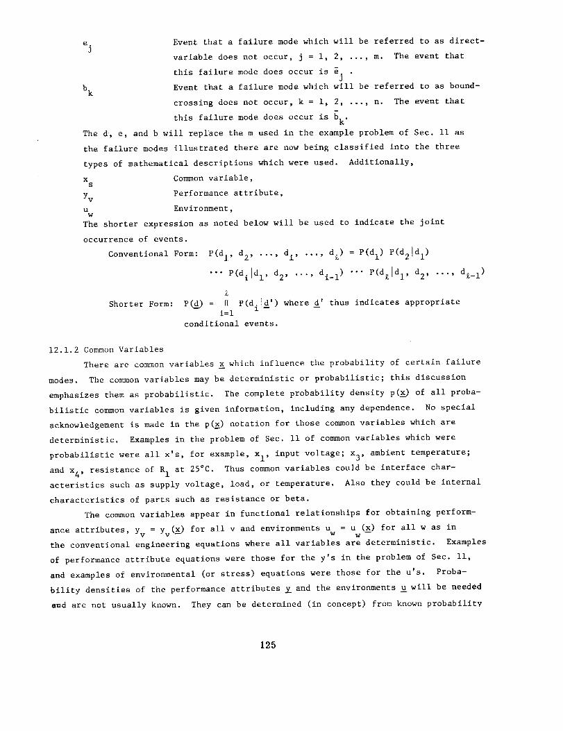
e. Event that a failure mode which will be referred to as direct-J
variable does not occur, j = i, 2, ..., m. The event that
this failure mode does occur is e.J
b k Event that a failure mode which will be referred to as bound-
crossing does not occur, k = i, 2, ..., n. The event that
failure mode does occur is bk"this
The d, e, and b will replace the m used in the example problem of Sec. ii as
the failure modes illustrated there are now being classified into the three
types of mathematical descriptions which were used. Additionally,
x Common variable,S
Yv Performance attribute,
u Environment,W
The shorter expression as noted below will be used to indicate the joint
occurrence of events.
Conventional Form:
Shorter Form:
P(dl, d2, ..., di, ..., d£) = P(d I) P(d21d I)
•-" P(dildl, d 2 .... , di_ I) "'" P(d£1dl, d 2, ..., d£_ I)
= H P(dild' ) where d' thus indicates appropriateP(d)i=l
conditional events.
12.1.2 Common Variables
There are common variables x which influence the probability of certain failure
modes. The common variables may be deterministic or probabilistic; this discussion
emphasizes them as probabilistic. The complete probability density p(_) of all proba-
bilistic common variables is given information, including any dependence. No special
acknowledgement is made in the p(_) notation for those common variables which are
deterministic. Examples in the problem of Sec. ii of common variables which were
probabilistic were all x's, for example, Xl, input voltage; x3, ambient temperature;
and x4, resistance of R 1 at 25°C. Thus common variables could be interface char-
acteristics such as supply voltage, load, or temperature. Also they could be internal
characteristics of parts such as resistance or beta.
The common variables appear in functional relationships for obtaining perform-
ance attributes, Yv yv(_) for all v and environments u = u (x) for all w as inW W --
the conventional engineering equations where all variables are deterministic. Examples
of performance attribute equations were those for the y's in the problem of Sec. ii,
and examples of environmental (or stress) equations were those for the u's. Proba-
bility densities of the performance attributes _ and the environments _ will be needed
end are not usually known. They can be determined (in concept) from known probability
125
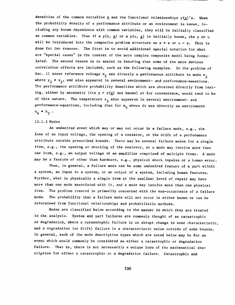
densities of the common variables _ and the functional relationships y(_)'s. When
the probability density of a performance attribute or an environment is known, in-
cluding any known dependence with common variables, they will be initially classified
as common variables. Thus if a p(y, _) or a p(u, _) is initially known, the y or u
will be introduced into the composite problem structure as y = x or u = x. This is
done for two reasons. The first is to avoid additional special notation for what
are "special cases" in the context of the more complex composite model being formu-
lated. The second reason is to assist in insuring that some of the more devious
correlation effects are included, such as the following examples. In the problem of
Sec. ii zener reference voltage x 2 was directly a performance attribute in mode m 2
where Y2 = x2' and also appeared in several environment_ and performance-equations.
The performance attribute probability densities which are obtained directly from test-
ing, either by necessity (its y = y(_) not known) or for convenience, would tend to be
of this nature. The temperature x 3 also appeared in several environment- and
performance-equatlons, including that for m 5 where it was directly an environment
u4 = x3 •
12.1.3 Modes
An undesired event which may or may not occur is a failure mode, e.g., the
loss of an input voltage, the opening of a resistor, or the drift of a performance
attribute outside prescribed bounds. There may be several failure modes for a single
item, e.g., the opening or shorting of the resistor, or a mode may involve more than
one item, e.g., an output voltage of an amplifier comprised of multiple items. A mode
may be a feature of other than hardware, e.g., physical shock impulse or a human error.
Thus, in general, a failure mode can be some undesired feature of a part within
a system, an input to a system, or an output of a system, including human features.
Further, what is physically a single item at the smallest level of repair may have
more than one mode associated with it, and a mode may involve more than one physical
item. The problem treated is primarily concerned with the non-occurrence of a failure
mode. The probability that a failure mode will not occur is either known or can be
determined from functional relationships and probabilistic methods.
Modes are classified below according to the manner in which they are treated
in the analysis. System and part failures are commonly thought of as catastrophic
or degradation, where a catastrophic failure is an abrupt change in some characteristic,
and a degradation (or drift) failure is a characteristic value outside of some bounds.
In general, each of the mode description types which are noted below may be for an
event which would commonly be considered as either a catastrophic or degradation
failure. That is, there is not necessarily a unique form of the mathematical des-
cription for either a catastrophic or a degradation failure. Catastrophic and
126
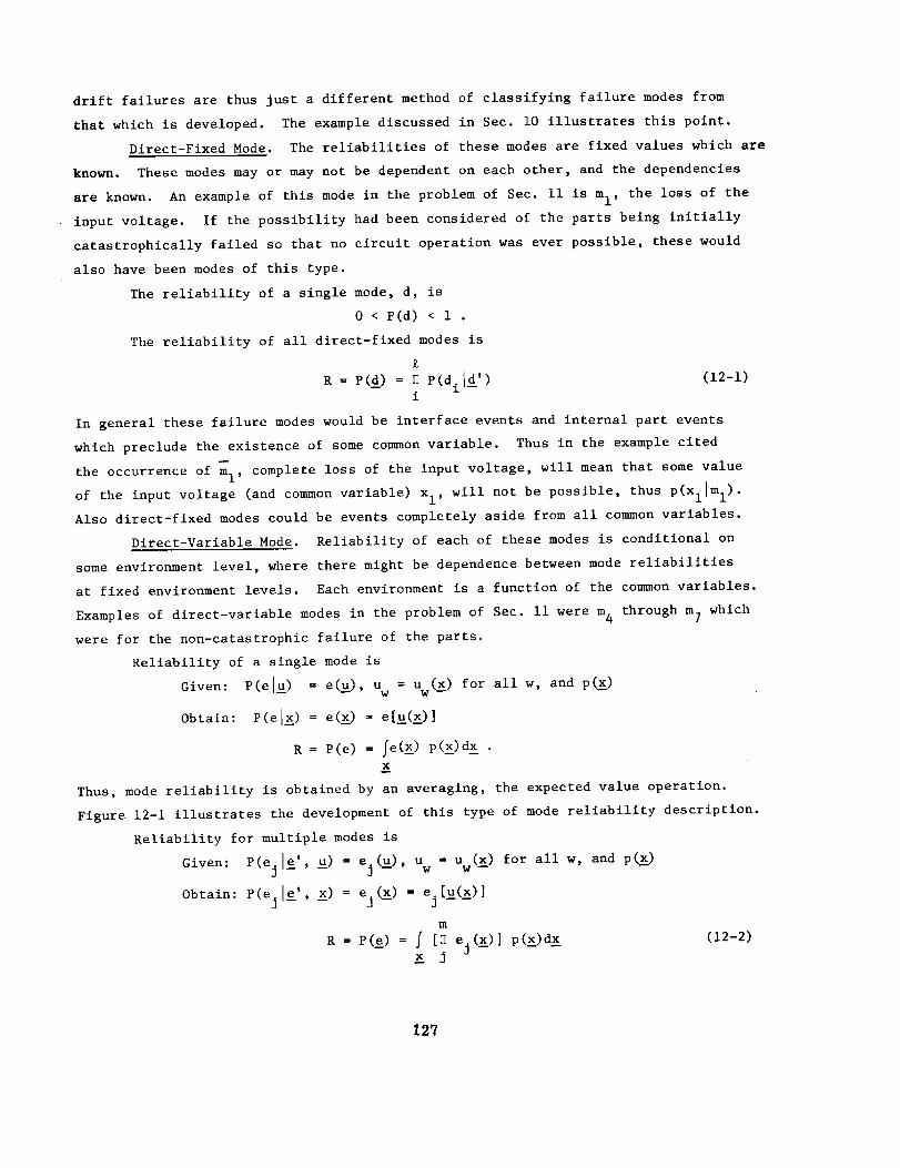
drift failures are thus just a different method of classifying failure modes from
that which is developed. The example discussed in Sec. i0 illustrates this point.
Direct-Fixed Mode. The reliabillties of these modes are fixed values which are
known. These modes may or may not be dependent on each other, and the dependencies
are known. An example of this mode in the problem of Sec. ii is m I, the loss of the
input voltage. If the possibility had been considered of the parts being initially
catastrophically failed so that no circuit operation was ever possible, these would
also have been modes of this type.
The reliability of a single mode, d, is
0 < P(d) < 1 .
The reliability of all direct-fixed modes is
£
R = P(d) = H P(d il_') (12-1)i
In general these failure modes would be interface events and internal part events
which preclude the existence of some common variable. Thus in the example cited
the occurrence of _i' complete loss of the input voltage, will mean that some value
of the input voltage (and common variable) x I, will not be possible, thus P(Xllml).
Also direct-fixed modes could be events completely aside from all common variables.
Direct-Variable Mode. Reliability of each of these modes is conditional on
some environment level, where there might be dependence between mode reliabillties
at fixed environment levels. Each environment is a function of the common variables.
Examples of direct-variable modes in the problem of Sec. ii were m 4 through m 7 which
were for the non-catastrophic failure of the parts.
Reliability of a single mode is
Given: e(el_) = e(_) u = Uw(X) for all w, and p(_)' W
Obtain: P(el_) = e(_) = e[_(_)]
R = P(e) = fe(_) p(x)dx .
X
Thus, mode reliability is obtained by an averaging, the expected value operation.
Figure 12-1 illustrates the development of this type of mode reliability description.
Reliability for multiple modes is
Given: P(ej le', u) = ej(u), uw = Uw(X)
Obtain: P(ejle' , _x) = e.(x)3-- --ej[u(x)]
m
R = e(e) = f [II ej(x)] p(x) dx_x j
for all w, and p_)
(12-2)
12'/
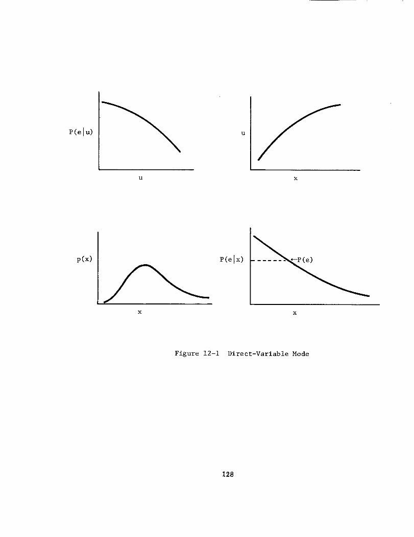
P(elu)
U X
p(x) P(elx)
X X
Figure 12-1 Direct-Variable Mode
128
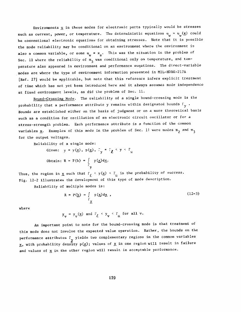
Environments _ in these modes for electronic parts typically would be stresses
such as current, _ power, or temperature. The deterministic equations u = u (x) couldW W --
be conventional electronic equations for obtaining stresses. Note that it is possible
the mode reliability may be conditional on an environment where the environment is
also a common variable, or some u = x . This was the situation in the problem ofw s
Sec. ii where the reliability of m 5 was conditional only on temperature, and tem-
perature also appeared in environment and performance euqations. The direct-variable
modes are where the type of environment information presented in MIL-HDBK-217A
[Ref. 27] would be applicable, but note that this reference infers explicit treatment
of time which has not yet been introduced here and it always assumes mode independence
at fixed environment levels, as did the problem of Sec. ii.
Bound-Crossing Mode. The reliability of a single bound-crossing mode is the
probability that a performance attribute y remains within designated bounds FY
Bounds are established either on the basis of judgment or on a more theoretical basis
such as a condition for oscillation of an electronic circuit oscillator or for a
stress-strength problem. Each performance attribute is a function of the common
variables _. Examples of this mode in the problem of Sec. ii were modes m 2 and m 3
for the output voltages.
Reliability of a single mode:
Given: y = y(x), p(_), F = F_ < y < F-- y u
Obtain: R = V(b) = / p(a)d_.F
Y
Thus, the region in x such that F1 < y(x) < r is the probability of success.
Fig. 12-2 illustrates the development of this type of mode description.
Reliability of multiple modes is:
R = e(_) = f p(_)dx , (12-3)
F
where
Yv = Yv (_) and £I < Yv < £ for all v.u
An important point to note for the bound-crossing mode is that treatment of
this mode does not involve the expected value operation. Rather, the bounds on the
performance attributes F yields two complementary regions in the common variables2
_, with probability density p(_); values of _ in one region will result in failure
and values of x in the other region will result in acceptable performance.
129
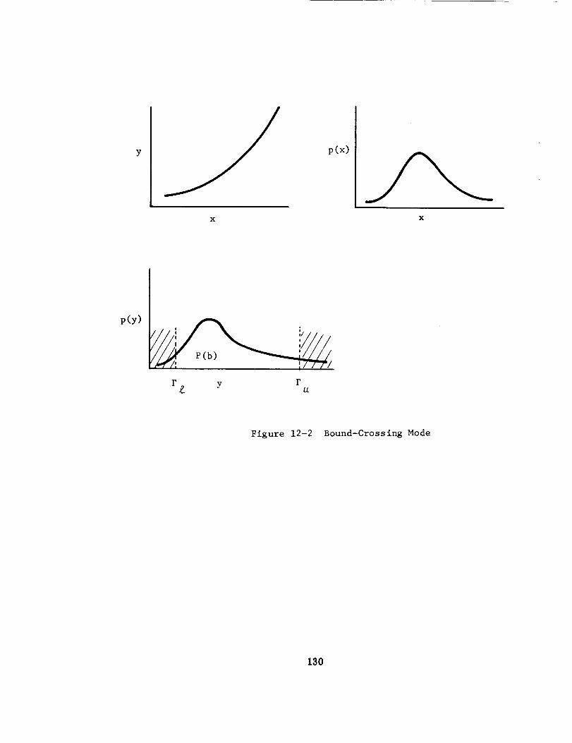
y p(x)
X X
P(Y)
F y F£ u
Figure 12-2 Bound-Crossing Mode
130
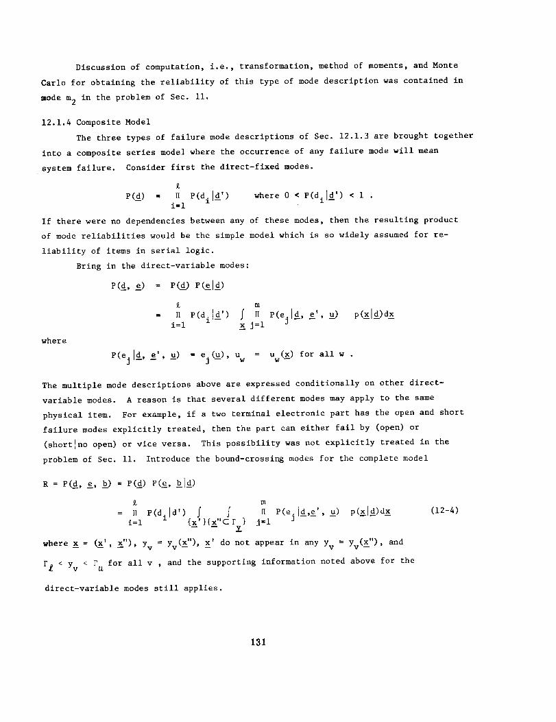
Discussion of computation, i.e., transformation, method of moments, and Monte
Carlo for obtaining the reliability of this type of mode description was contained in
mode m 2 in the problem of Sec. ii.
12.1.4 Composite Model
The three types of failure mode descriptions of Sec. 12.1.3 are brought together
into a composite series model where the occurrence of any failure mode will mean
system failure. Consider first the direct-flxed modes.
P(d) = H e(dild') where 0 • P(dild') < i .i=l
If there were no dependencies between any of these modes, then the resulting product
of mode reliabilities would be the simple model which is so widely assumed for re-
liability of items in serial logic.
Bring in the direct-variable modes:
P(_, i) = P(!) P(_Ig)
m
= H P(dil_' ) f H P(ejl_, _', _) p(_Id)dxi=l _ j=l
where
P(ej Id, _e', u) = e=j(u),_ Uw -- Uw(X)_ for all w .
The multiple mode descriptions above are expressed conditionally on other direct-
variable modes. A reason is that several different modes may apply to the same
physical item. For example, if a two terminal electronic part has the open and short
failure modes explicitly treated, then the part can either fail by (open) or
(shortlno open) or vice versa. This possibility was not explicitly treated in the
problem of Sec. ii. Introduce the bound-crossing modes for the complete model
R = P(d, e, b) = P(d) P(e, b ld)
m
= H P(dild') f f H P(ej Id,e', u) p(xld)dxi=l {x'}{_x"cr } j=l
= _x_") ' -- "where _x = (x', _x"), Yv Yv _ , x do not appear in any Yv Yv (x)' and
F£ < Yv < FU for all v , and the supporting information noted above for the
(12-4)
dlrect-variable modes still applies.
131
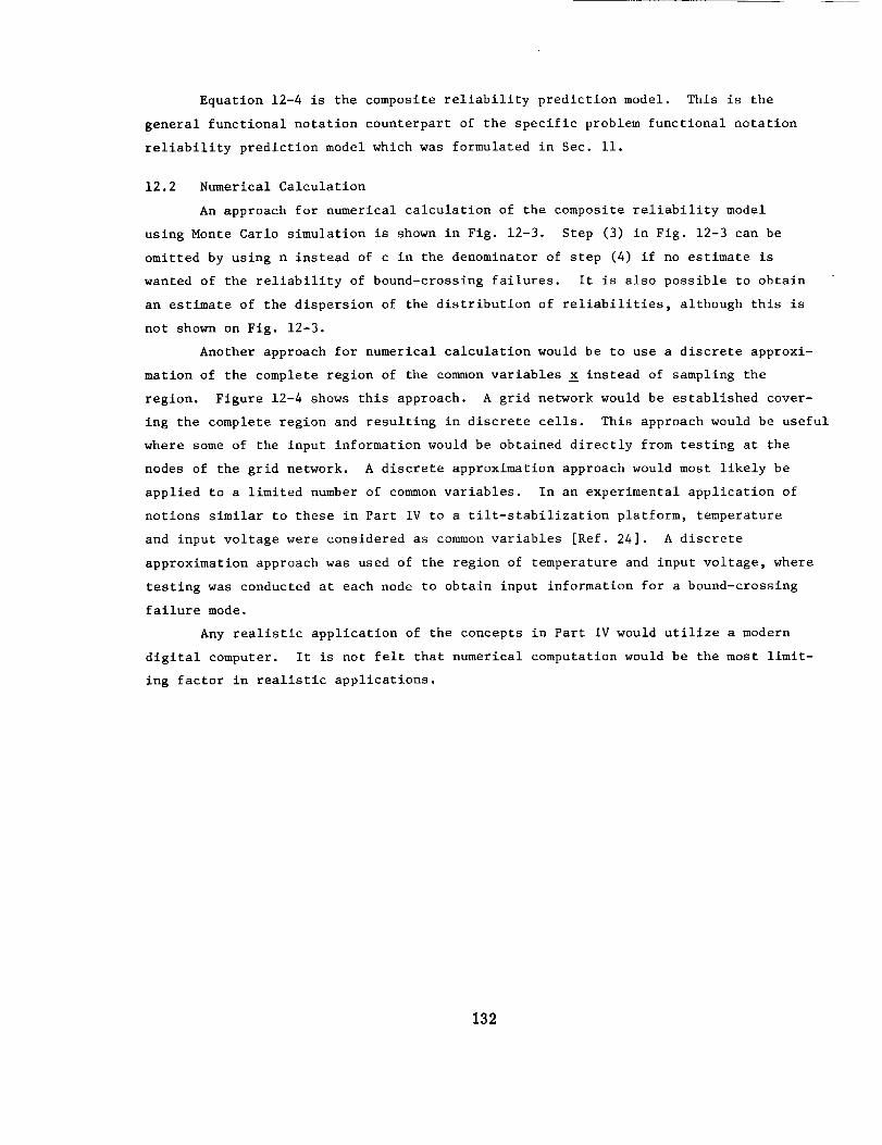
Equation 12-4 is the composite reliability prediction model. This is the
general functional notation counterpart of the specific problem functional notation
reliability prediction model which was formulated in Sec. ii.
12.2 Numerical Calculation
An approach for numerical calculation of the composite reliability model
using Monte Carlo simulation is shown in Fig. 12-3. Step (3) in Fig. 12-3 can be
omitted by using n instead of c in the denominator of step (4) if no estimate is
wanted of the reliability of bound-crossing failures. It is also possible to obtain
an estimate of the dispersion of the distribution of reliabilities, although this is
not shown on Fig. 12-3.
Another approach for numerical calculation would be to use a discrete approxi-
mation of the complete region of the common variables _ instead of sampling the
region. Figure 12-4 shows this approach. A grid network would be established cover-
ing the complete region and resulting in discrete cells. This approach would be useful
where some of the input information would be obtained directly from testing at the
nodes of the grid network. A discrete approximation approach would most likely be
applied to a limited number of common variables. In an experimental application of
notions similar to these in Part IV to a tilt-stabilization platform, temperature
and input voltage were considered as common variables [Ref. 24]. A discrete
approximation approach was used Of the region of temperature and input voltage, where
testing was conducted at each node to obtain input information for a bound-crossing
failure mode.
Any realistic application of the concepts in Part IV would utilize a modern
digital computer. It is not felt that numerical computation would be the most limit-
ing factor in realistic applications.
132
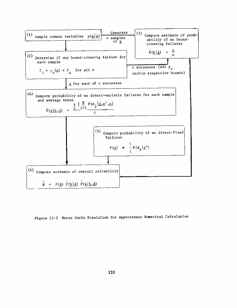
(1)
(2) Determine if any
each sample
Generate (3) Compute estimate of prob-Sample common variables p(_]d) n samples
of x ability of no bound-
- crossing failures
, *,_,_,-P(_l_)- c
bound-crossing failure for]_ n
L-._--_--..-------J
< for all v I c successes (all Yv
F_ Yv(_) < _ ] within respective bounds)
i_ for each of successesc
I
Compute probability of no direct-varlable failures for each sample I
and average these E [ _ P I_,_' ,_] i_(elb,d) _ c j=l (ej
(4)
(5)Compute probability of no direct-fixed
failures
P (d_)
' 1
(6) Compute estimate of overall reliabilit_
E p (di id' )i
R : _(d) 5(bld) P(__Ib,d_)
Figure 12-3 Monte Carlo Simulation for Approximate Numerical Calculation
133
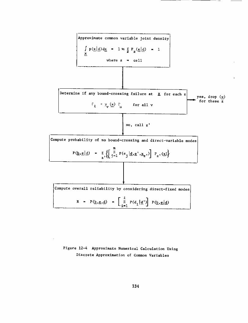
Approximate common variable joint density
f p(xld)dx = 1 _ zE ez(xld)__ = 1X
where z = cell
Determine if any bound-crossing failure at
F£ < Yv (x)- Pa for all v
_x!
for each Z lyes ' drop (_)
r for these z
no, call z'
Compute probability of no bound-crossing and dlrect-variable modes
m
r. H (x_)1P(b'eld) = z,{[J=iP(ej'd'e''X--z ')] Pz'
R = P(b,e,d) = 11 P(dl}d'i=l
overall reliability by considering direct-flxed modes
Figure 12-4 Approximate Numerical Calculation Using
DiscreteApproximatlon of Common Variables
134
12.3 Additional Considerations
Questions naturally arise concerning extensions to explicitly treating
time and to parallel situations. The essence of the approach has been illus-
trated thus far, and brief comments are given below on these questions. The
comments are brief and qualitative because mathematical notation becomes even
• more complex. Some key features are noted which would be useful to one seriously
pursuing the problem. That is; one will have to develop the detail and these features
are noted for guidance.
12.3.1 Explicitly Treating Time
As might be expected, explicitly treating time in the series situation
model is a reasonably straightforward extension of the approach used in Sec. 12.1.
The concept of common variables and of the three types of mode descriptions remains
unchanged. Mathematical descriptions of reliability measures as functions of time
for the direct modes would be as described in Secs. 4.2 and 4.3 and of time-varying
probability density functions for common variables and performance attributes would
be as described in Sec. 5.4. Thus, for common variables the time dependence is
denoted by p_; t) and for a particular variable x (t) = x (_; t) for all s, where p(_)s s
is the pdf of the constants, _ = (al, a2, ..., an).
Nothing unique exists about the direct-fixed mode. There would be great
practical difficulty in obtaining the direct-variable mode reliability descriptions
conditional on a time-varying environment
P[ej(t)Id , e', _(t)].
This would result from the general situation that a large variety of possible forms
of _(t) are possible. It is, therefore, difficult to develop tables or other standard
information for general use with time-varying environments. A situation which is more
practical is where the direct-variable mode reliabilities are functions of time, but
the probability densities of the common variables and thus the time varying environ-
ments are not functions of time, i.e., conventional failure rate graphs of Ref. 27.
The bound-crossing mode will have the unique feature that there could be a specific
failure time for each possible value of a (where _ is that noted above for the common
variables). This will have the effect of entering into the composite model as trun-
cations on the reliability time-functions of the direct-variable modes. Both mono-
tonic and some non-monotonic performance attribute variations could be treated, as
they both become first-crossing problems.
135
12.3.2 Parallel Models
The situation where the occurrence of certain failure modes does not mean
system failure will be referred to as the parallel one. Before proceding to more
involved considerations it is pertinent to note that the expected value operation
as cited in Sec. 9.1 can be applied to conventional reliability models for redundancy
where the environment is a probabilistic variable. This straightforward approach is
useful in certain practical problems. Where the complexities of Sec. 12.1 are present,
branching modeling concepts could be used. First, the series situation model of 12.1
would be structured where there are no failure modes. For other non-failed system
states some of the input information may be different than for the system-state where
there are no failure modes. For instance, some common variables could take on values
of zero, and performance attribute and environment equations could change. System-
state change sequences would have to be traced, and a detailed reliability prediction
model developed for each sequence. Where time is explicitly treated, the time that
system-state changes will occur is an explicit variable, and time-wlse convolutions
could be used in tracing through the detail. Thus, explicit treatment of time in
redundancy situations would significantly increase complexity.
136
13. Concluding Remarks for Part IV
Each number below refers to the corresponding question noted in the introduction
to Part IV. Replies to these questions are intended to serve as concluding remarks
to Part IV. The replies take into consideration mainly the material presented in
Part IV.
(i) The first question concerns the conventional assumption of probabilistic
independence in reliability models. The probabilistic dependence treated in Part
IV results from various sources. Consider first the series model: (a) the most
straightforward dependence occurs in the given conditional probabilities in the direct-
fixed and the direct-varlable modes. (b) the common variables can bring about depend-
ence among direct-variable modes in addition to that noted in (a), dependence
among bound-crossing modes, and dependence between direct-variable and bound-crossing
modes.
Also to be noted here is to avoid confusing probabilistic dependence with error
in structuring the problem. Where there is a deterministic relation y = y(x) between
a performance attribute and common variables, and if some of the common variables
were forced to be treated as modes in that some judgment-based bound was put on each
of these common variables and the functional relationship ignored, then simply the
erroneous reliability prediction would be ohtalned. Additional dependence is introduced
when a general parallel model is developed as features of the series model may be
conditional on the system state.
(2) A key feature in structuring the composite reliability prediction models
of Sec. 12 is recognition of the distinction between failuremodes, common variables,
performance attributes_ and environments. This distinction is of the sort which
tends to be obvious in hind-sight but was not beforehand. A distraction seems to
be a tendency to want to treat separately different real-world features which are
really mathematically similar in the sense of structuring the composite reliability
prediction model. For example, for electrical equipment there is a tendency to separate
the internal part characteristics from the interface characteristics.
(3) The typical deterministic equations of engineering have been divided into
two categories, those concerned with performance attributes and those concerned with
environments. The performance attribute equations are used for the bound-crossing
mode. A performance attribute may be either an output of the system or it may be
some internal performance of the system. The latter is not of interest to the system
user, but there may be certain bounds within which the internal performance must
remain or else the output(s) of the system, which are of interest to the user, will
be affected. The environment equations are used in the direct-variable mode.
137
4) The discussion in Sec. i0 illustrated that there is no l-to-i correspondence
between classification of a failure at a point of repair (source) into catastrophic
or degradation and a similar two-way classification of the manner in which the system
performance is affected. The models which are developed in Sec. 12 are based on
a classification system concerning the mathematlcal manner by which an individual
failure mode is described, and do not emphasize the classification system of catastrophic
and degradation failures.
(5) The composite models developed and presented in Sec. 12 show how the various
features are brought together. These composite models do not resemble the more familiar
prediction models which are widely used. Bringing the various failure mode types
and common variables together for even a simple series situation is shown to be com-
plex. Note also that the composite model includes many of the slngle-item reliability
measures of Part II and the conventional reliability models of Part III.
(6) The complexity of the composite reliability models in Sec. 12 and the gen-
eral lack of necessary input data combine to support the current practices of using
simpler models. It is posslhle that there may be problems where some features of the
composite model would offer some return which would be worth the effort. Certain
relatively simple systems which have high safety implications might warrant more com-
plex analyses. An example might be relatively simple devices concerned with explosives,
such as detonation circuits. The need for high reliability might Justify the efforts
necessary to develop the appropriate data. Another possible application area would
be at a systems level with regard to redundancy. This would be as discussed in
Sec. 12.3.2 concerning the use of the expected value operation for redundancy where
some features of the composite model are dropped. In some situations there may be
some value in using features of the composite model in efforts to achieve balance in
design with regard to efforts to reduce various failure modes. In such cases little
emphasis would be given to the absolute numerical value of the reliabillty prediction
number, but rather the values would be compared for different design approaches. Also
note that in a real-world problem, it may be that only a small number of the variables
present in the problem will require treatment in the depth implied by the detailed
model.
Generally speaking, experimental applications and further investigation are
necessary in order to determine if more complex reliability prediction models along
these lines have anything to offer in a practical sense. Of course, before such
investigations can be attempted it is necessary that an approach to structuring the
problem be developed, and this necessary first step was an objective of the investi-
gations reported in Part IV.
138

Motivation for pursuing detailed reliability prediction models includes main-
tainability objectives as well as reliability ones. A detailed reliability model
might eventually be useful for maintainability improvements concerning automated
predictive maintenance, test point selection, and repair procedure development. These
potential maintainability uses would generally require models for parallel con-
figurations.
139
APPENDIX
Mathematics of Prediction - Probability
The calculus of probability plays an important part in the prediction of
system reliability. The basic definitions and distribution theory (discrete and
continuous-univariate and multivariate) play a basic role. The Boolean algebra and
the calculus of probabilities provide the appropriate analytical tools for manipu-
lating these probabilistic inputs. In the calculation of a probability of system
behavior there is little choice in the simplifying approaches that can be taken
except to use some of the reliability bounds and approximations. Even to use these
techniques requires a formal introduction to the basic methods and a thorough under-
standing of the assumptions implied in their use.
In order to make the written material as brief as possible Summary tables
have been prepared to cover specific topics such as continuous variables, Boolean
algebra, calculus of probabilities, etc. Supporting each of these tables are cited
references, discussions and examples demonstrating the techniques in the correspond-
ing table. Appendix references are contained along with all other references in the
single reference section.
140
A.I Continuous Random Variables and Distributions
A continuous random variable is typically one that can take on any value in an
interval. For example, the lifetime of a transistor under a certain set of test
conditions could be any time greater than zero. For a very large population of
transistors one would expect the lives to be scattered or distributed over a large
interval of time. Continuous distribution functions are used to describe such
statistical behavior. Table A.I-I summarizes basic concepts concerning continuous
random variables and their distributions. A summary of several common distributions
is presented in Table A.I-2. Given a density function p(x) the characteristics can
be evaluated by application of the formulae in Table A.I-I.
Central Limit Theorem
One of the most important results in statistics is the central limit theorem (CLT)
which states that if x l, x 2, ..., Xn are independent random variables al_ having the
same distribution function F(x) with mean _ and standard deviation o, then the sum
n
S = _ X.
ii=l
is asymptotically Normally distributed with mean np and standard deviation o_n, i.e.,
so
_ f -i 21 exp{ _ (s - n_) }dsP(s < so ) 2,/_-_o_n
for n sufficiently large. This result is true under very general conditions on F(x);
if all variables have the same distribution then it is sufficient that the second
moment of x be finite. A more general form of the CLT and additional discussion of
the above case appear in Ref. 52.. An important aspect of the theorem is how large
n must be before the normal approximation applies. Clearly this dependence on n is
conditioned by the shape of the distribution. Sums of variables having highly
skewed distributions would tend to Normality more slowly than for those having
symmetrical or more nearly Normal distributions. In the latter case sums of variables
with n larger than 25 or 30 are very closely approximated by the Normal distribution.
141
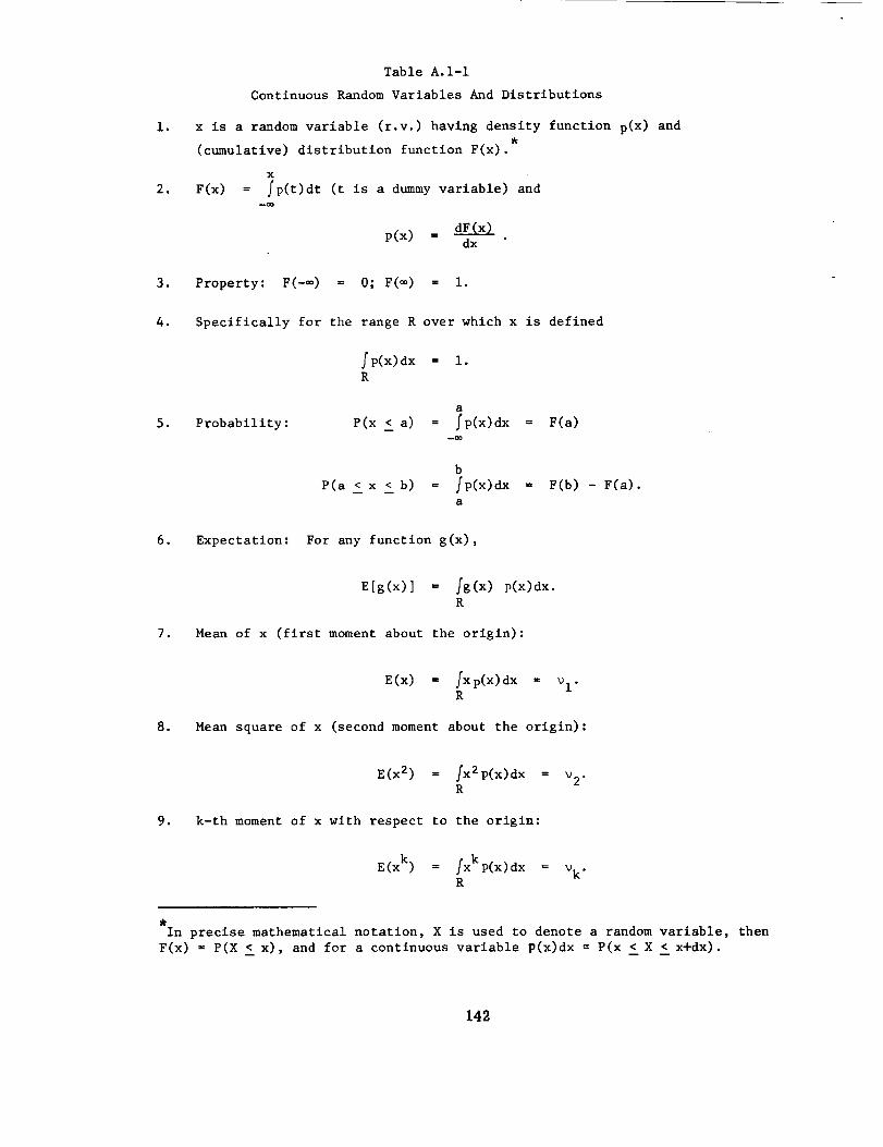
i,
2,
Table A. i-i
Continuous Random Variables And Distributions
x is a random variable (r.v.) having density function p(X) and
(cumulative) distribution function F(x).
X
F(x) = fp(t)dt (t is a dummy variable) and
p(x) = dF(x)dx
3,
4.
5,
Property: F(-®) = 0; F(_) = i.
Specifically for the range R over which x is defined
fp(x)dx = i.R
a
Probability: P(x <__a) = fp(x)dx = F(a)
b
P(a < x < b) = /p(x)dx = F(b) - F(a).
a
6. Expectation: For any function g(x),
E[g(x) ] = fg(x) p(x)dx.
R
7. Mean of x (first moment about the origin):
8,
E(X) = fx p(x) dx = _i"R
Mean square of x (second moment about the origin):
E(x2) -- fx2p(x)dx = v2"R
9. k-th moment of x with respect to the origin:
E(xk) = /xkp(x)dx = _k"R
In precise mathematical notation, X is used to denote a random variable, then
F(x) = P(X ! x), and for a continuous variable p(x)dx = P(x ! X ! x+dx).
142
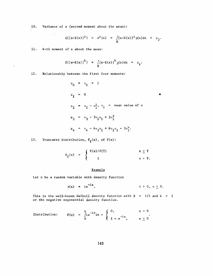
i0. Variance of x (second moment about the mean):
11.
E{ [x-E(x) ]2 } = °2(x) = /[x-E(x) ]2 P(x)dx = _2"R
k-th moment of x about the mean:
12.
E{[x-E(x)]k} = /[x-E(x)]kp(x)dx = _k"R
Relationship between the first four moments:
P0 = _0 = i
_ = 0
P2 = _2 - _' _i = mean value of x
_3 = 93 - 392_i + 2_
_4 = 94 - 4_3_i + 69291 - 39_.
13. Truncated distribution, FT(X) , of F(x):
FT(X) = { F(x)/F(T) x <__T1 x> T.
Example
Let x be a random variable with density function
-_xp(x) = he , _ > 0, x > 0.
This is the well-known Weibull density function with 8 = I/% and k = I
or the negative exponential density function.
Distribution:x -At _ 0, x < 0
F(x) = Jle dt = 1 -hE0 l-e , x>0
143
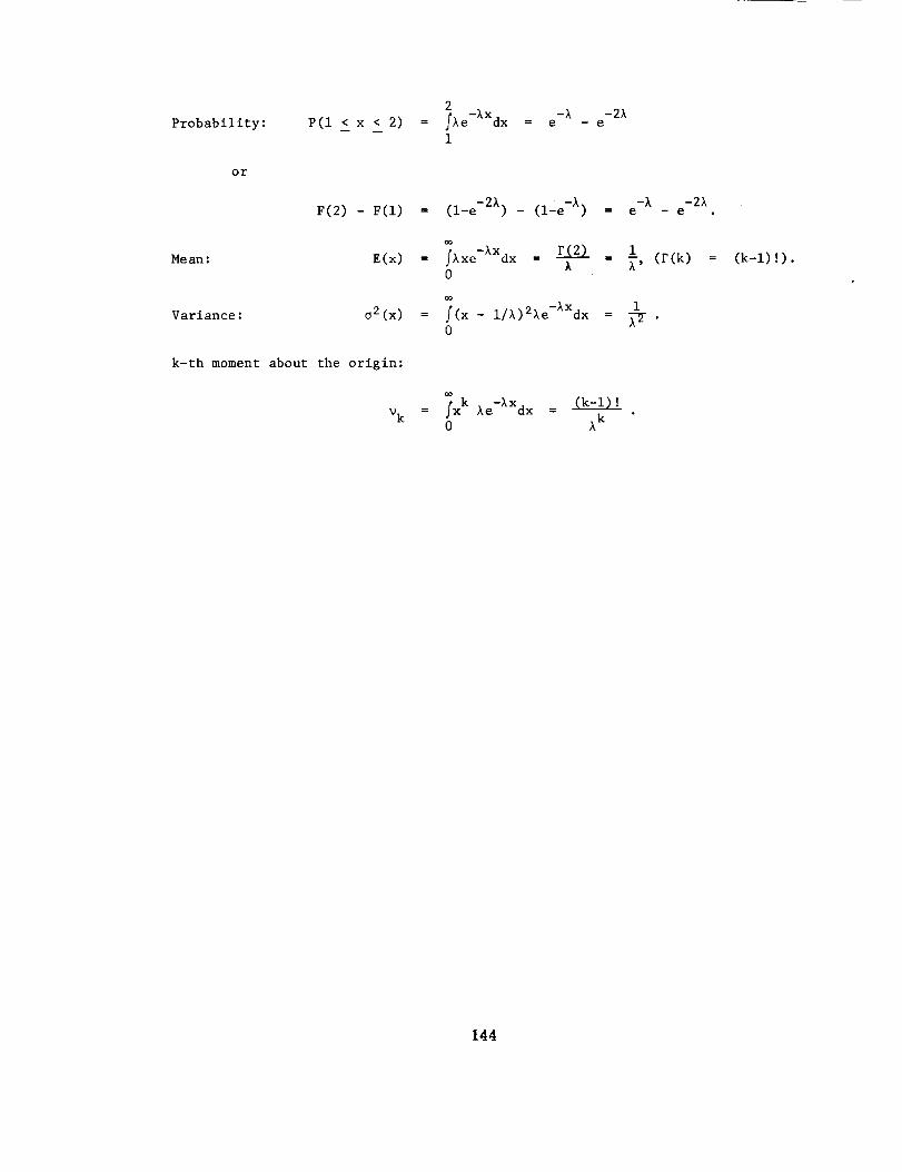
Probability: }le-lXdx -21P(I < x < 2) = = e -I - e
1
or
-I -21F(2) - F(1) = --(l-e-21) - --(l'e-l ) = e - e
Mean: E(x) = _Jlxe-lXdxr(2) 1
= l - l' (r(k) = (k-l)!).0
Variance:
Oo
i02(x) = f(x- i/l)21e-lXdx = l--_-.
0
k-th moment about the origin:
oo
_k = /xk le-lXdx =0 I k
144
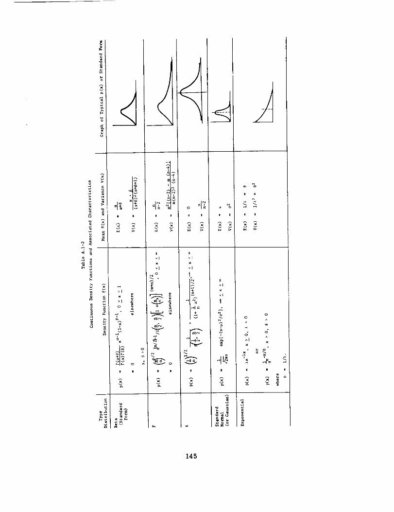
P.
v
.,,,.q
.,., +_ _+
i_ °
0
_.o<.1
_o
o ._
_o
.-q
vl
o
v
0
_v
I IN
v
a=n ,..
I
| II
8
vl0
+
,,,-0
_o| II
n I n u
8
"1
vl
,_ e,i
,"_1 "
v
8
vl
vl
%
I
N
I I1
• -4 ,--t
N H
_ v
00
^^
An^1
I I I
-,-t
145
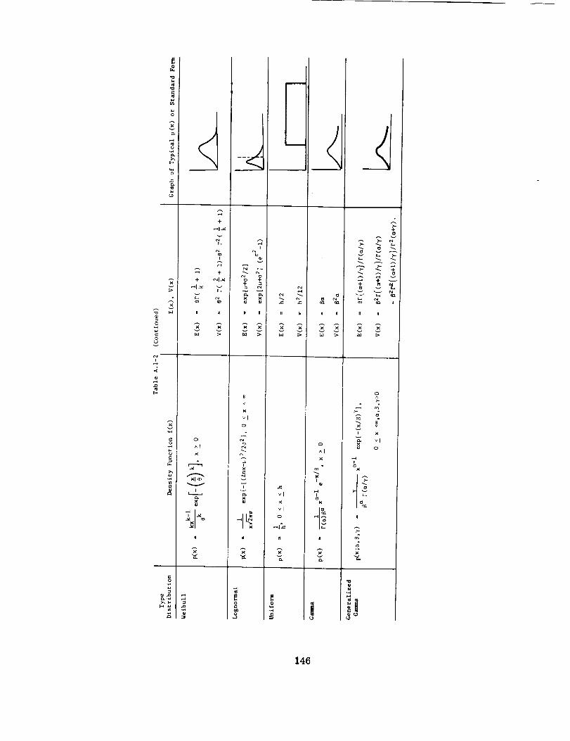
m
,i.i
v
,++
+
,-+I +_
v
%,.-+
,_ + <r','l_v ,..-41 ._
+-.C _'<:,:, %
_ o•,..i A I
g .
II
%(U
v
II
8
v
vlo
_2
e4
x
v
i
w
¢-
vIX
"l0
fl
v
H
0
^1X
H
v
_ + _
. _<vl
0
v
%
il
<_
.°
146
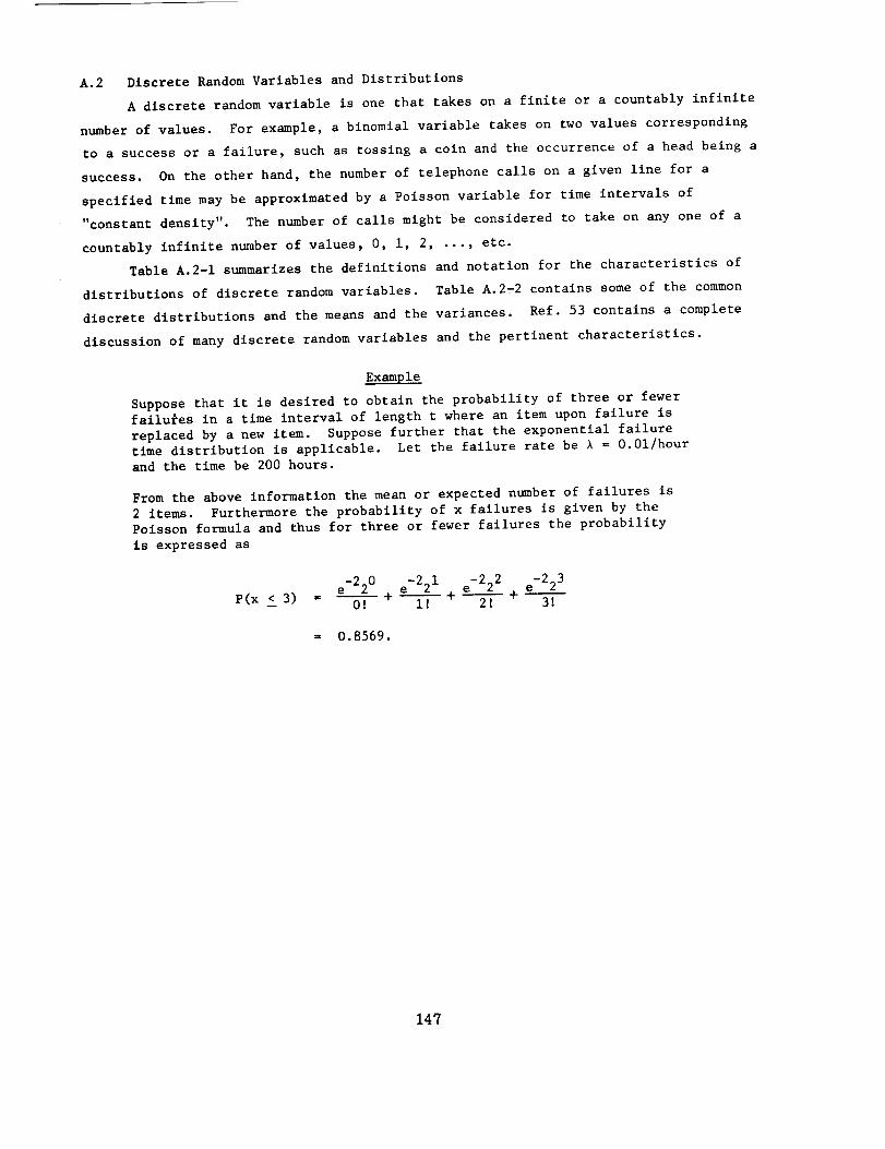
A.2 Discrete Random Variables and Distributions
A discrete random variable is one that takes on a finite or a countably infinite
number of values. For example, a binomial variable takes on two values corresponding
to a success or a failure, such as tossing a coin and the occurrence of a head being a
success. On the other hand, the number of telephone calls on a given line for a
specified time may be approximated by a Poisson variable for time intervals of
"constant density". The number of calls might be considered to take on any one of a
countably infinite number of values, 0, i, 2, ..., etc.
Table A.2-1 summarizes the definitions and notation for the characteristics of
distributions of discrete random variables. Table A.2-2 contains some of the common
discrete distributions and the means and the variances. Ref. 53 contains a complete
discussion of many discrete random variables and the pertinent characteristics.
Example
Suppose that it is desired to obtain the probability of three or fewer
failures in a time interval of length t where an item upon failure is
replaced by a new item. Suppose further that the exponential failure
time distribution is applicable. Let the failure rate be X = 0.01/hour
and the time be 200 hours.
From the above information the mean or expected number of failures is
2 items. Furthermore the probability of x failures is given by the
Polsson formula and thus for three or fewer failures the probability
is expressed as
e-220 e-221 e-222 e-223
e(x ! 3) = 0----_+ i----_+ 2----_+ 3----_
= 0.8569.
147
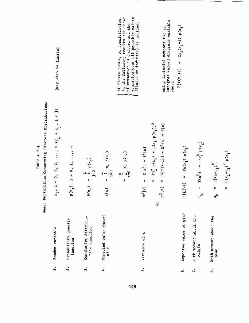
m
o
4-i
U
,-I .H
oq
0L)
0
4a
U
t0
4J
0
gv
v
oe-)
v
X
8
,-4
I!
,-.4
E_0
8
II
v
:>.,4-1
m
:>,,,
•,-I O
.Q U
O
/-%
_4
O-,-I_ II
II
I
._
•H °r-I";3 _J
U
•_-I u.-i
,-4 0
g-
Xv
O8 [,,._1 II
gv
,-4
"O
_q
v
OI_ i.-,-,,_ II
.,-4
v +
I I
I _v I
v
II II II
0
0
U
.,.4
_4
,-I
0 _'
_1 t# vEl t0 ._0 .W
_1 _ II
1.+ .-I0 _1
(J ,--4_1_-4 I
•,_ _ _I
:_.,_
v
v
v
0
,-.4
.IJ
v
II
v
II
IJ
0
0 "H
OI
I
v
II
O
gO
I
v
,-.4
I
v
148
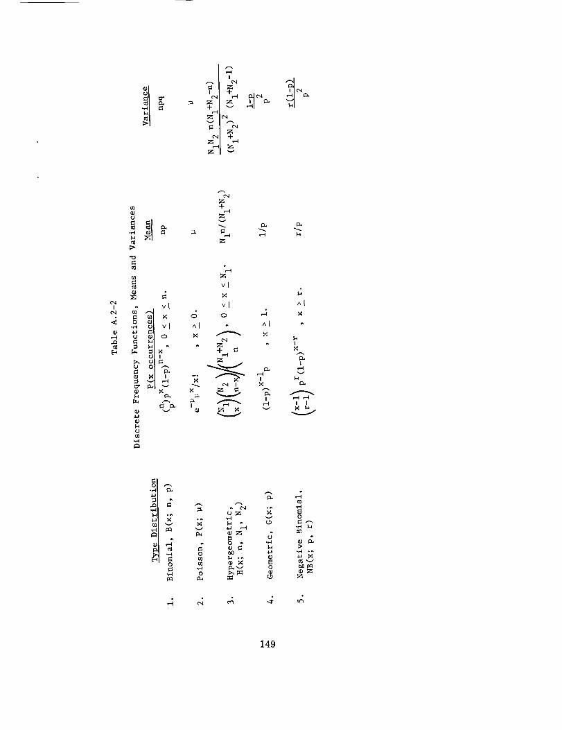
I
Zv
z_z_
Icq
o4
Z
o4
o_
(D
Zv
Z
Z
vl
vl vl
vl ^1 _ ^1
_ I
^I
I
I
I I
0
.el
,'_ ,g
_._ _ -_-I
0 _D ___ -,-I•
._ _'--_ 0 _D _C_0 _ _ _Z
_ _D Z
149
A.3 Multivariate Distributions (Emphasis on Bivariate Case)
Consider the situation in which two or more measurements on a part are being
obtained, e.g. the equivalent h-parameters of a transistor. These two measurements
would have a joint probability density function (pdf) p(x, y), say, where x and y
denote the respective measurements. If the two variables are statistically independ-
ent then
p(x, y) = Pl(X) P2 (y) '
and hence the joint density functions can be written down knowing the individual pdf's.
If the variables are not independent the multivariate density function can be obtained
by assuming a particular form such as the Normal density function and estimating the
unknown parameters from available data.
Most of the properties of bivariate (two-variate) distributions are straight-
forward generalizations of the univariate distributions given earlier. The new
concepts are those of conditional and marginal distributions, covariance and correla-
tion. The generalization of these results to multivariate distributions is easily
made and one should see Ref. 51 for these results.
Independent Random Variables. If two variables x and y are independent then
the covariance of x and y, denoted by Coy(x, y) is
Cov(x, y) =//(x-E(x)) Pl(X)(y-E(y)) p2(Y)dxdy = 0.
However the inverse is not true, i.e. two variables may have zero covariance (or zero
correlation i.e. @(x, y) = 0) but not be independent. For example, suppose that
u and v are independent variables, and let x = u + v, y = u - v. Then
E(xy) = E(u 2) - E(v 2) = 0, E(y) = 0, and
Cov(x, y) = 0 and O(X, y) = 0.
However, x and y are dependent. See Ref. 17 for additional examples. Thus the
correlation is not a general measure of dependence but rather a measure of linear
dependence of two variables in physical terms; the correlation coefficient is a
dimensionless covariance.
150
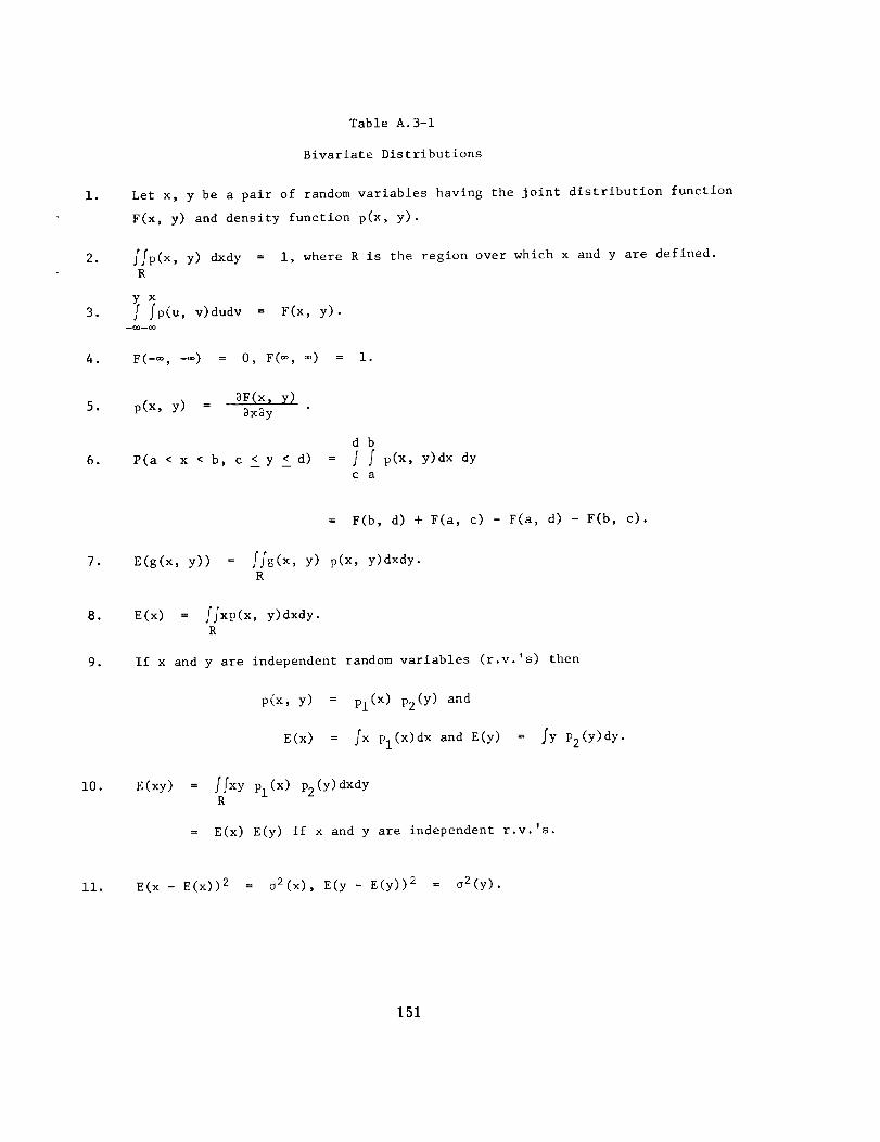
i,
2Q
3..
Table A.3-1
Bivariate Distributions
Let x, y be a pair of random variables having the joint distribution function
F(x, y) and density function p(x, y).
ffp(x, y) dxdy = i, where R is the region over which x and y are defined.R
X/p(u, v) dudv = F(x, y).--1=o--oo
4. F(--, --) = 0, F(_, _) = I.
_F(x, y)5. p(x, y) =
_x_y
db
6. P(a < x < b, c <_ y <__d) = ] / p(x, y)dx dy
C a
= F(b, d) + F(a, c) - F(a, d) - F(b, c).
7. E(g(x, y)) = //g(x, y) p(x, y)dxdy.
R
8. E(x) = ffxp(x, y)dxdy.
R
9. If x and y are independent random variables (r.v.'s) then
p(x, y) = Pl(X) p2(y) and
E(x) = /x Pl(X)dx and E(y) = /y p2(Y)dy.
I0. E(xy) = f/xy el(x) p2(Y)dxdyR
= E(x) E(y) if x and y are independent r.v.'s.
ii. E(x - E(x)) 2 = o2(x), E(y - E(y)) 2 = o2(y).
151
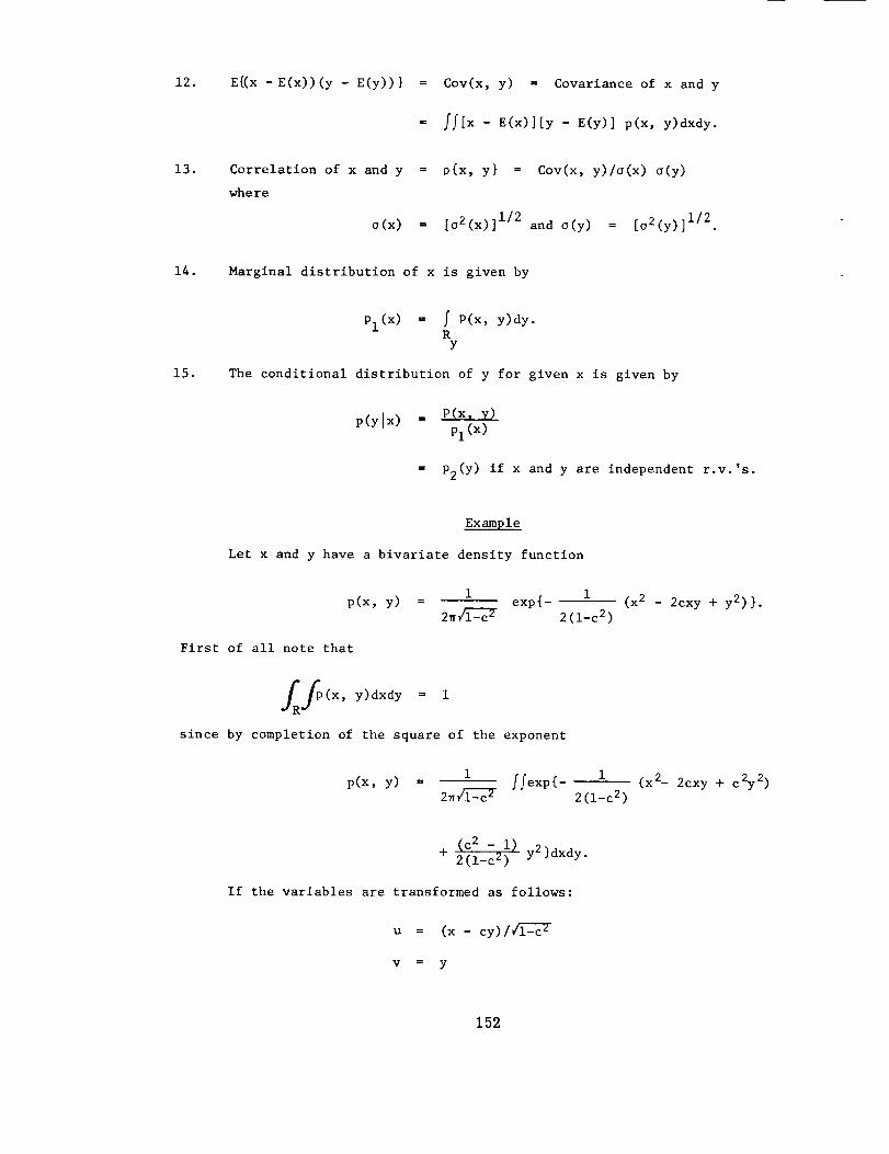
12. E{(x -E(x))(y - E(y))} = Cov(x, y) = Covariance of x and y
= If Ix - E(x)][y - E(y)] p(x, y)dxdy.
13. Correlation of x and y
where
= p{x, y} = Cov(x, y)/o(x) o(y)
g(x) = [o2(x)] I/2 and o(y) = [g2(y)] I/2
14. Marginal distribution of x is given by
15.
Pl(X) ffi f P(x, y)dy.RY
The conditional distribution of y for given x is given by
p(ylx ) = P(x, y)Pl (x)
= p2(y) if x and y are independent r.v.'s.
Example
Let x and y have a bivariate density function
ip(x, y) - exp{
1
2(I-c 2)
First of all note that
P(X, y)dxdy = I
since by completion of the square of the exponent
p(x, y) = i ffexp{2_-_
1
2(i-c 2 )
(x2 - 2cxy + y2)}.
(x 2- 2cxy + c_ 2)
(c 2 - l)+ 2(l_c 2) y2}dxdy •
If the variables are transformed as follows:
u = (x - cy)I/ir7r
v = y
152
then
p(u, v) -u2 v 2
1 ffexp{-( T+T )}du dv,2_
using the fact that the Jacobian of the transformation is given by
(A.3-I)
i/
3u _u
3x 3y
3v _v
8x 3y
= 1/
(A-3.1) can be written as the product of the integrals
u2 v 2Oo _ -- oo -- --
1 fe 2du • i____fe 2dv2_7_-_ 2_7_-_
1/ ¢iSc-Z - c / ¢i-s_
0 1
__ d-:h-z .
Since each is the integral of the standard Normal density function the above product
is unity.
Next the marginal distribution of y is given by
p2(y ) = fp(x, y)dx
1 exp{ - y2 }2
Hence the conditional distribution of x given y is
= i (x - cy)2}.p(x[y) = p(x, y) 1 exp{- 2(i_c2 )
P(Y) /2_(i-c 2)
Mean, Variance and Covariance Formulas
be n random variables with means B I, _2' "''' _n andLet x I, x 2, ..., x n
2 . 0 2 respectively and correlations PI2 (= P(Xl' x2))" 013' "'''variances o , 02 , .. , n
The following results are true independent of the distributions of the0n-l, n"
variables. Let y be a linear combination of the variables given by
X •
Y = cO + ClXl + c2x2 + "'" + Cn n
153
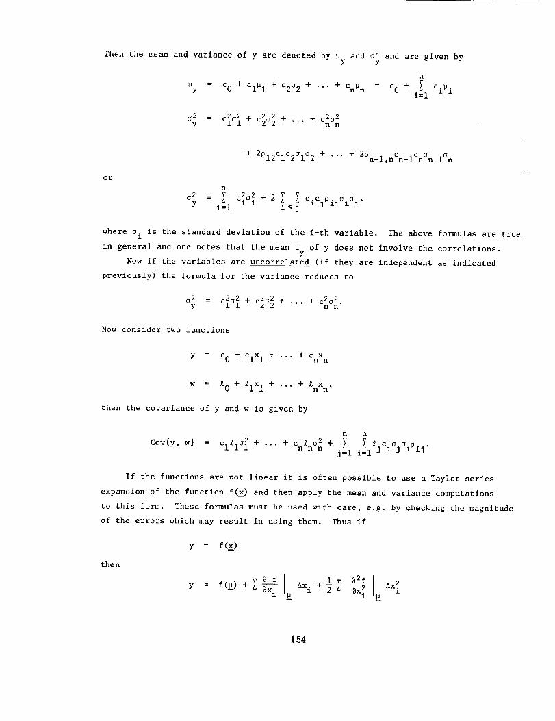
Then the mean and variance of y are denoted by _ and a 2 and are given byY Y
n
py -- c o + ClP 1 + c2P 2 + ... + CnP n = c o + [ eiP ii=l
o2 2 2 + 2 2 c2o2= c2o 2 + ... +Y Cl°l n n
+ 2P12ClC2OlO 2 + ... + 2Pn_l,nCn_iCnOn_lO n
or
n
0 2 _ 2 2 +2 _ _= cio i cicj 0ij °i°j
Y i=l i<j
where o i is the standard deviation of the i-th variable. The above formulas are true
in general and one notes that the mean _y of y does not involve the correlations.
Now if the variables are uncorrelated (if they are independent as indicated
previously) the formula for the variance reduces to
02 = 2 2 + 2 2 + . + C202y Cl°l c2°2 "" n n"
Now consider two functions
Y = co + c.x. + ... + c xU .t i n n
w = £0 + £1Xl + "'" + £nXn '
then the covariance of y and w is given by
n n
i "'" o2+ I l jCiOjoi ij.Coy{y, w} = ci£io + + Cn£n n j=l i-
If the functions are not linear it is often possible to use a Taylor series
expansion of the function f(_) and then apply the mean and variance computations
to this form. These formulas must be used with care, e.g. by checking the magnitude
of the errors which may result in using them. Thus if
y = f(_)
then
1 82f J Ax 28 f Axi +_[ 3x_= f(_) + _ _-_i _ __ 1
154
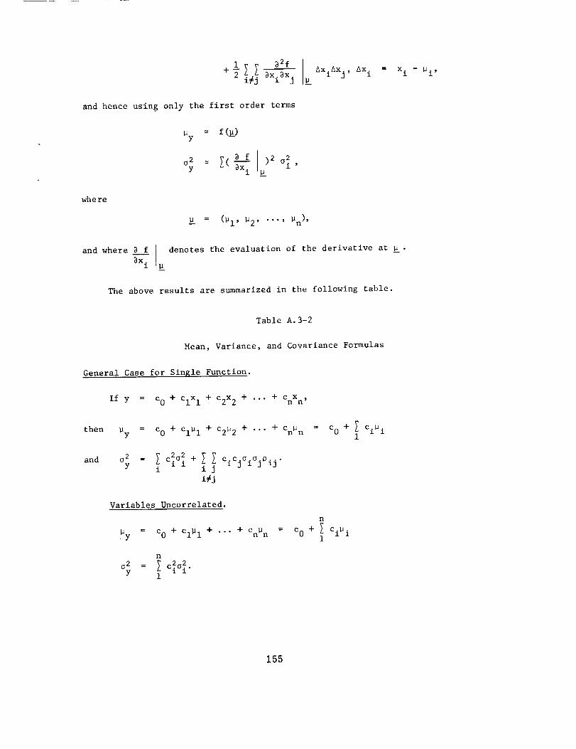
1 _2f I_xi--_-x j AxiAxj' Axi = xi - _i'
and hence using only the first order terms
wh e re
_y = f(_)
02 : _( 3 f I) 20_y _ l'
_-- = (_i' _2 .... ' _n )'
and where 3 f [ denotes the evaluation of the derivative at _.
_xi I__
The above results are summarized in the following table.
Table A. 3-2
Mean, Variance, and Covariance Formulas
General Case for Single Function.
If y = cO + ClX 1 + c2x 2 + +•.. CnX n,
then _y = co + Cl_ 1 + c2_ 2 + ... + Cn_ n = Co + { ci_i
= CiO i cicj °i°j Pij •Y i ij
i#j
and
Variables Uncorrelated.
by co + Cl_ 1 + ... + Cn_ n
n
02 _ 2 2= CiO i •Y 1
n
co + _ ci_i
155
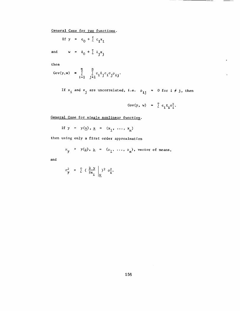
General Case for two functions.
and
If y = co + _ cix i
w = £0 + _ £jxj
then
n n
Cov(y,w) = _ _ici£joicjOij .i=l j=
If xi and xj are uncorrelated, i.e. Oi j
Coy(y, w)
General Case for single nonlinear function.
If y = y(x), x = (xl, ..., Xn)
then using only a first order approximation
and
= 0 for i # j, then
-- _ ci_io2.
Uy = Y(L), L = (_i' ..., Un ), vector of means,
y _x i _ m
156
A.4 Calculus of Probabilities
Starting with certain definitions and axioms several useful theorems of the
calculus of probabilities can be derived. Eight such theorems are given in Table A.4-1
A major difficulty in reliability literature stems from the notion of statistical
independence, often called just independence. This notion is basic to many reliability
calculations, for it is often assumed in these calculations that the failure of one
item in a system is independent of the failure of all other items in the system. In
non-probability language, two events are said to be independent if knowledge of the
outcome of one in no way affects the outcome of the other event. The simplest example
of independent events is perhaps two tosses of a coin - the result of the first toss
in no way affects the outcome of the second toss, so the events are independent.
As a more pertinent example, suppose two amplifiers are selected at random from a
collection of i00 amplifiers from a production process. Does knowledge concerning
the value of current gain for the first amplifier alter in any way the probability
that the current gain for the second amplifier falls in any given interval? If the
answer is that it does not, then the two observations of current gain are independent.
In applications these results would usually be treated as independent because if the
current gain distribution were F(x), the observation of an x I for the first amplifier
would not aid in locating the value x 2 for the second one as it presumably could fall
anywhere on the defined region R for x with the same probability distribution F(x) as
that for the first observation.
Consider as another example the measuring of the current gain Yc and the voltage
gain Yv of a single amplifier. Does knowledge of the value of current gain alter
information concerning the voltage gain? Chances are that it would because high
values of Yc may correspond to higher than average (or lower than average) values of
Yv and vice versa. Thus it is normally assumed that such variables may be dependent
unless data analyses imply otherwise.
Similar examples can be considered in the reliability prediction area. If the
event of failure of one of two items in parallel in no way affects the failure
behavior of the other item the two events are independent. On the other hand if
failure of one would alter the probability distribution of failure time of the
second item the two events of failure are dependent.
In probabilistic terms the above discussion can be summarized as follows.
A and B are independent if
and hence
P(BIA) = P(B)
P(AB) = P(BIA) P(A) ,, P(B) P(A),
whereP(BIA) is read "the probability of the event B given the event A has occurred."
Another consideration with respect to independence is that of statistical
independence and conditional independence which has been denoted as physical
independence in Ref. 54.
Two events A and B are said to be conditionally (physically) independent if
and only if they are statistically independent under environment Ei' that is,
P(XYIEI) = P(X[Ei) P(Y[E i)
Physlcal (conditional) independence does not necessarily imply statistical independence
of the unconditional events X and Y. In order to compute the reliability of a system
one usu@lly obtains the conditional probabilities (that is, given the environments)
and then obtains the weighted average of these conditional probabilities using the
P(E i) as the weights. In mathematical terms
P(XY) = [ P(XYIEi) P(Ei) ,i
or
P(XY) = _ P(XIEi) P(YIEi) P(Ei).i
Frequently in reliability prediction the mission is subdivided into phases in each
of which the environment is essentially constant throughout the entire phase. Hence
one uses a formula such as the above. A more complete discussion of the concepts of
physical and statistical independence appears in Ref. 48 and Ref. 54.
158
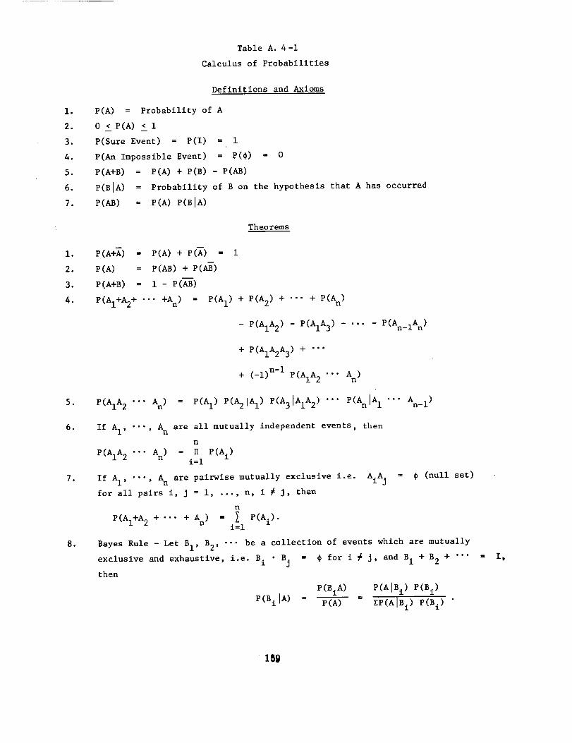
Table A. 4-i
Calculus of Probabilities
io
2.
3.
4.
5.
6.
7.
2.
3.
4.
5,
6.
,
8,
Definitions and Axioms
P(A) = Probability of A
0 < P(A) < 1
P(Sure Event) _ P(1) = i
P(An Impossible Event) = P(_)
P(A+B) = P(A) + P(B) - P(AB)
P(BIA)
P(AB)
-- 0
= Probability of B on the hypothesis that A has occurred
= P(A) P(BIA)
Theorems
P(A+A) = P(A) + P(A--) = 1
P(A) = P(AB) + P(AB)
P(A+B) = i - P(AB)
P(AI+A2+ -.. +An) = P(AI) + P(A2) + ... + P(An)
- P(AIA2) - P(AIA3) ..... P(An_IA n)
+ P(AIA2A 3) + ...
+ (-1) n-I P(AIA 2 "'' An)
P(AIA 2 ..- An) = P(AI) P(A2IA I) P(A3IAIA 2) "-- P(AnIA 1 "-" An_ 1 )
If A I, •'- , An are all mutually independent events, then
n
P(AIA 2 "'" A n ) = E P(A i)i=l
If A I, "'', An are pairwise mutually exclusive i.e. AiA i = _ (null set)
for all pairs i, J = i, ..., n, i # J, then
n
P(AI+A 2 + ... + An ) " [ P(Ai)"i=l
Bayes Rule - Let BI, B2, .-. be a collection of events which are mutually
exclusive and exhaustive, i.e. B i • Bj
then
= _ for i # J, and B I + B 2 + .... I,
P(Bi IA) P(A)
P(BiA) P(AIBi ) P(Bi)
= - rP(AIBi) P(Bi)
159
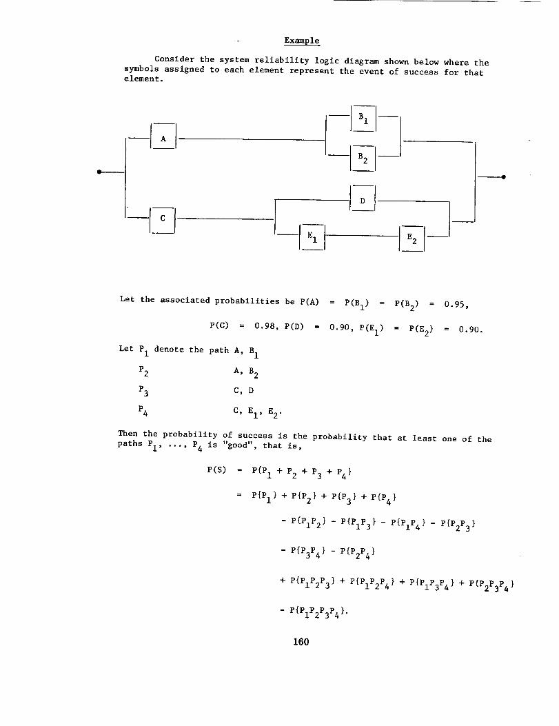
Example
Consider the system reliability logic diagram shown below where the
symbols assigned to each element represent the event of success for thatelement.
kq1 1
Let the associated probabilities be P(A) = P(BI) = P(B2) = 0.95,
P(C) = 0.98, P(D) = 0.90, P(EI) = P(E 2) = 0.90.
Let P1 denote the path A, B 1
P2 A, B 2
P3 C, D
P4 C, El, E2.
Then the probability of success is the probability that at least one of the
paths PI' "''' P4 is "good", that is,
P(S) = P{PI + P2 + P3 + P4 }
= P(PI } + P{P2 } + P{P3} + P{P4 }
- P(PIP2 } - P{PIP3} - P(PIP4} - P{P2P3 }
- P(P3P4 } - P{P2P4 }
+ P{PIP2P3 } + P{PIP2P4} + P{PIP3P4 } + P(P2P3P4}
- P{PIP2P3P4}.
160
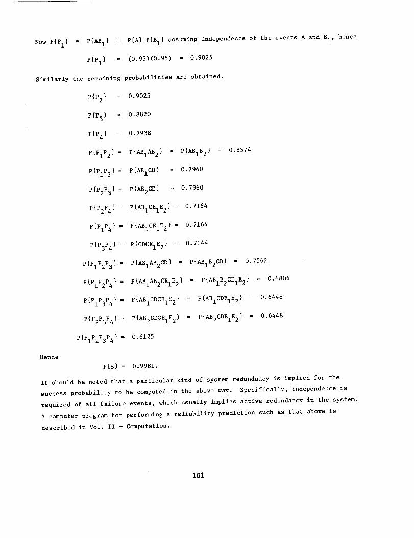
Now P{PI } = P{AB I} = P{A} P{B I} assuming independence of the events A and B I, hence
P{PI } = (0.95)(0.95) = 0.9025
Similarly the remaining probabilities are obtained.
P{P2 } -- 0.9025
P{P3 } = 0.8820
P{P4 } = 0.7938
p{piP2 } = P{ABIAB 2} = P{ABIB 2} = 0.8574
p{pIP3 } -- P{ABICD} = 0.7960
p{p2P3} = P{AB2CD} = 0.7960
p{p2P4} = P(ABICEIE 2} = 0.7164
p{pIP4} = P{ABICEIE 2} = 0.7164
p{p3P4 } = P{CDCEIE 2} = 0.7144
p{piP2P3} = P{ABIAB2CD} = P{ABIB2CD} = 0.7562
p{piP2P4 } = P{ABIAB2CEIE 2 } = P[ABIB2CEIE 2 } = 0.6806
p{piP3P4 } = P{ABICDCEIE2} -- P{ABICDEIE 2} = 0.6448
p{p2P3P4 } = P{AB2CDCEIE 2} = P{AB2CDEIE 2} = 0.6448
P {PIP2P3P4 } = 0.6125
Hence
P{S} = 0.9981.
It should be noted that a particular kind of system redundancy is implied for the
success probability to be computed in the above way. Specifically, independence is
required of all failure events, which usually implies active redundancy in the system.
A computer program for performing a reliability prediction such as that above is
described in Vol. II - Computation.
161
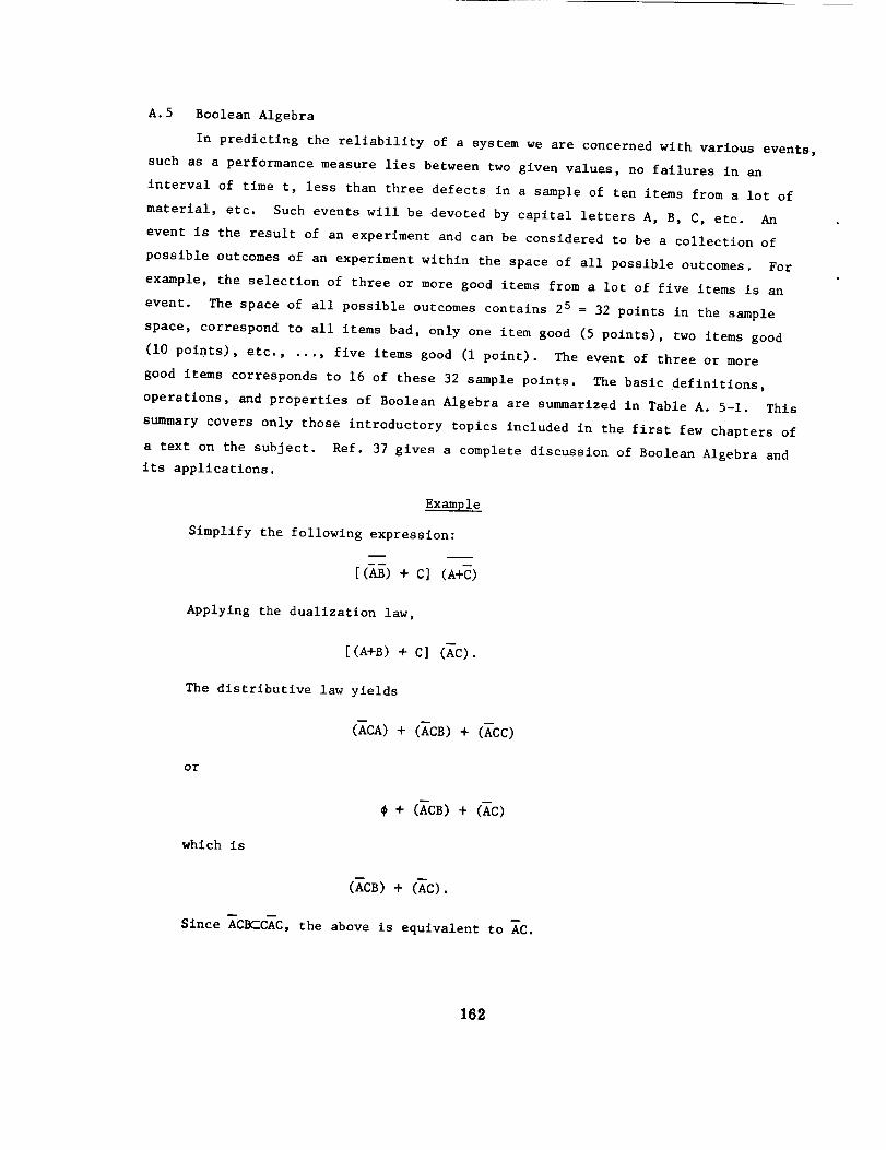
A.5 Boolean Algebra
In predicting the reliability of a system we are concerned with various events,
such as a performance measure lies between two given values, no failures in an
interval of time t, less than three defects in a sample of ten items from a lot of
material, etc. Such events will be devoted by capital letters A, B, C, etc. An
event is the result of an experiment and can be considered to be a collection of
possible outcomes of an experiment within the space of all possible outcomes. For
example, the selection of three or more good items from a lot of five items is an
event. The space of all possible outcomes contains 25 = 32 points in the sample
space, correspond to all items bad, only one item good (5 points), two items good
(I0 points) , etc., ..., five items good (i point). The event of three or more
good items corresponds to 16 of these 32 sample points. The basic definitions,
operations, and properties of Boolean Algebra are summarized in Table A. 5-1. This
summary covers only those introductory topics included in the first few chapters of
a text on the subject. Ref. 37 gives a complete discussion of Boolean Algebra and
its applications.
Example
Simplify the following expression:
[(_) + c] (A+C)
Applying the dualizatlon law,
[(A+B) + C] (AC).
The distributive law yields
(A--CA) + (A--CB)+ (ACC)
or
which is
+ (A--CB)+ (AC)
(A--CB) + (AC).
Slnce ACBCCAC, the above is equivalent to AC.
162
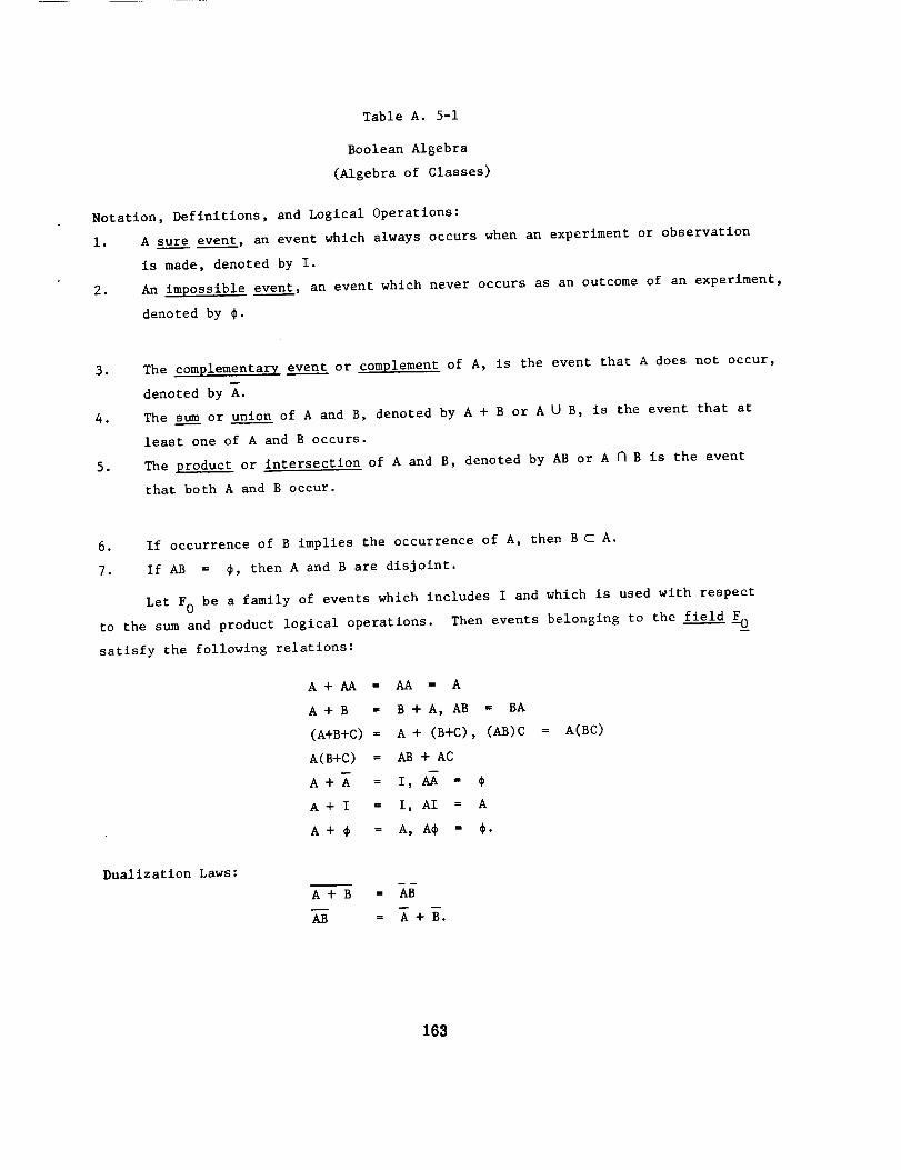
Table A. 5-1
Boolean Algebra
(Algebra of Classes)
Notation, Definitions, and Logical Operations:
1. A sure event, an event which always occurs when an experiment or observation
is made, denoted by I.
2. An impossible event, an event which never occurs as an outcome of an experiment,
denoted by _.
3,
4.
.
The complementarz event or complement of A, is the event that A does not occur,
denoted by A.
The sum or union of A and B, denoted by A + B or A U B, is the event that at
least one of A and B occurs.
The product or intersection of A and B, denoted by AB or A N B is the event
that both A and B occur.
6. If occurrence of B implies the occurrence of A, then B C A.
7. If AB = #, then A and B are disjoint.
Let F0 be a family of events which includes I and which is used with respect
to the sum and product logical operations. Then events belonging to the field _O
satisfy the following relations:
A + AA = AA = A
A + B = B + A, AB = BA
(A+B+C) = A + (B+C), (AB)C
A(B+C) = AB + AC
A + A = I, AA =
A + I = I, AI = A
A + _ = A, A_ = _.
= A(BC)
Dualization Laws:
A+ B = AB
AB = A+B.
163
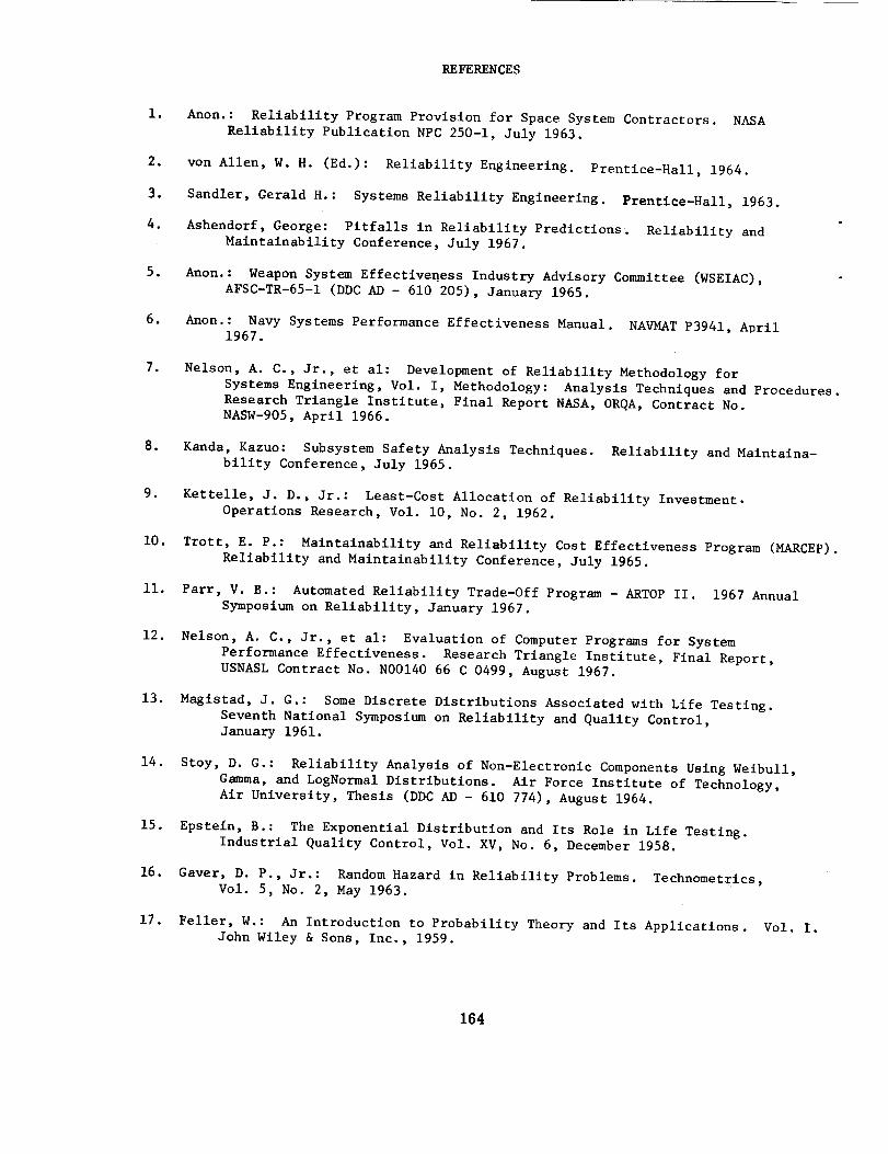
REFERENCES
1. Anon.: Reliability Program Provision for Space System Contractors. NASA
Reliability Publication NPC 250-1, July 1963.
2. yon Allen, W. H. (Ed.): Reliability Engineering. Prentice-Hall, 1964.
3. Sandler, Gerald H.: Systems Reliability Engineering. Prentlce-Hall, 1963.
. Ashendorf, George: Pitfalls in Reliability Predictions. Reliability and
Maintainability Conference, July 1967.
. Anon.: Weapon System Effectiveness Industry Advisory Committee (WSEIAC),
AFSC-TR-65-1 (DDC AD - 610 205), January 1965.
6. Anon.: Navy Systems Performance Effectiveness Manual. NAVMAT P3941, April1967.
. Nelson, A. C., Jr., et al: Development of Reliability Methodology for
Systems Engineering, Vol. I, Methodology: Analysis Techniques and Procedures.
Research Triangle Institute, Final Report NASA, ORQA, Contract No.
NASW-905, April 1966.
. Kanda, Kazuo: Subsystem Safety Analysis Techniques. Reliability and Maintaina-
bility Conference, July 1965.
. Kettelle, J. D., Jr.: Least-Cost Allocation of Reliability Investment.
Operations Research, Vol. i0, No. 2, 1962.
i0. Trott, E. P.: Maintainability and Reliability Cost Effectiveness Program (MARCEP).
Reliability and Maintainability Conference, July 1965.
ii. Parr, V. B.: Automated Reliability Trade-Off Program - ARTOP II. 1967 Annual
Symposium on Reliability, January 1967.
12. Nelson, A. C., Jr., et al: Evaluation of Computer Programs for System
Performance Effectiveness. Research Triangle Institute, Final Report,
USNASL Contract No. NO0140 66 C 0499, August 1967.
13. Magistad, J. G°: Some Discrete Distributions Associated with Life Testing.
Seventh National Symposium on Reliability and Quality Control,
January 1961.
14. Stoy, D. G.: Reliability Analysis of Non-Electronic Components Using Weibull,
Gamma, and LogNormal Distributions. Air Force Institute of Technology,
Air University, Thesis (DDC AD - 610 774), August 1964.
15. Epstein, B.: The Exponential Distribution and Its Role in Life Testing.
Industrial Quality Control, Vol. XV, No. 6, December 1958.
16. Gaver, D. P., Jr.: Random Hazard in Reliability Problems. Technometrics ,
Vol. 5, No. 2, May 1963.
17. Feller, W.: An Introduction to Probability Theory and Its Applications. Vol. I.
John Wiley & Sons, Inc., 1959.
164
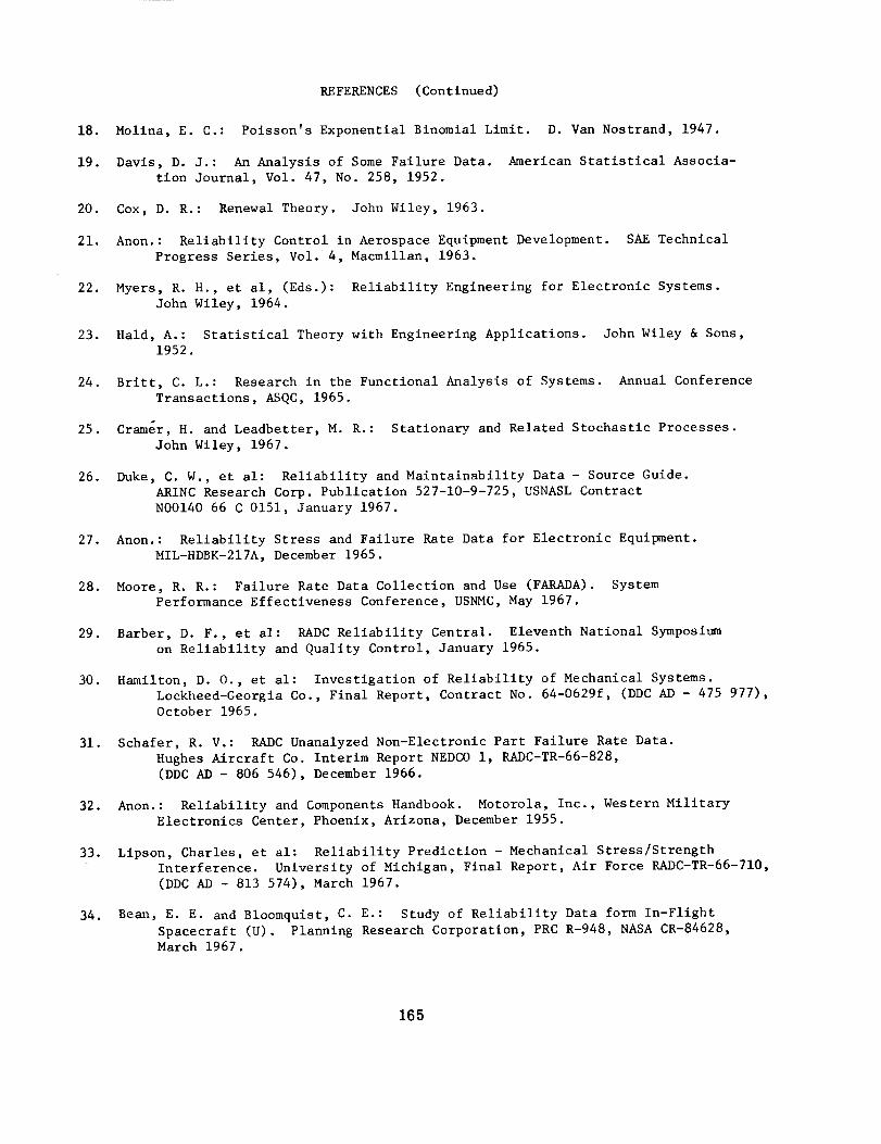
REFERENCES (Continued)
18. Molina, E. C.: Poisson's Exponential Binomial Limit. D. Van Nostrand, 1947.
19. Davis, D. J.: An Analysis of Some Failure Data. American Statistical Associa-
tion Journal, Vol. 47, No. 258, 1952.
20. Cox, D. R.: Renewal Theory. John Wiley, 1963.
21. Anon.: Reliability Control in Aerospace Equipment Development. SAE Technical
Progress Series, Vol. 4, Macmillan, 1963.
22. Myers, R. H., et al, (Eds.): Reliability Engineering for Electronic Systems.
John Wiley, 1964.
23. Hald, A.: Statistical Theory with Engineering Applications. John Wiley & Sons,
1952.
24. Britt, C. L.: Research in the Functional Analysis of Systems. Annual Conference
Transactions, ASQC, 1965.
25. Cramer, H. and Leadbetter, M. R.: Stationary and Related Stochastic Processes.
John Wiley, 1967.
26. Duke, C. W., et al: Reliability and Maintainability Data - Source Guide.
ARINC Research Corp. Publication 527-10-9-725, USNASL Contract
N00140 66 C 0151, January 1967.
27. Anon.: Reliability Stress and Failure Rate Data for Electronic Equipment.
MIL-HDBK-217A, December 1965.
28. Moore, R. R.: Failure Rate Data Collection and Use (FARADA). System
Performance Effectiveness Conference, USNMC, May 1967.
29. Barber, D. F., et al: RADC Reliability Central. Eleventh National Symposium
on Reliability and Quality Control, January 1965.
30. Hamilton, D. O., et al: Investigation of Reliability of Mechanical Systems.
Lockheed-Georgia Co., Final Report, Contract No. 64-0629f, (DDC AD - 475 977),
October 1965.
31. Schafer, R. V.: RADC Unanalyzed Non-Electronic Part Failure Rate Data.
Hughes Aircraft Co. Interim Report NEDCO i, RADC-TR-66-828,
(DDC AD - 806 546), December 1966.
32. Anon.: Reliability and Components Handbook. Motorola, Inc., Western Military
Electronics Center, Phoenix, Arizona, December 1955.
33. Lipson, Charles, et al: Reliability Prediction - Mechanical Stress/Strength
Interference. University of Michigan, Final Report, Air Force RADC-TR-66-710,
(DDC AD - 813 574), March 1967.
34. Bean, E. E. and Bloomquist, C. E.: Study of Reliability Data form In-Flight
Spacecraft (U). Planning Research Corporation, PRC R-948, NASA CR-84628,March 1967.
165
REFERENCES (Continued)
35. Allen, G. H., et al: Multi-Discipline Approach for Achieving Operational
Reliability. 1967 Annual Symposium on Reliability, January 1967.
36. Muller, F.W.: Elementary Reliability Technology. Sandla Corp. Monograph,
SC-R-64-198, July 1964.
37. Flegg, H. G.: Boolean Algebra and Its Application. John Wiley & Sons, 1965.
38. Braverman, J. D., et al: Reliability Modeling with Conditional Probability
Logic. 1966 Annual Symposium on Reliability, January 1966.
39. Messinger, M., et al: Rellability Approximations for Complex Structures.
1967 Annual Symposium on Reliability, January 1967.
40. Krohn, C. A., et al: Methods of Design Stage Reliability Analysis. 1967
Annual Symposium on Reliability, January 1967.
41. Bazovsky, Igor: Reliability: Theory and Practice. Prentice-Hall, 1961.
42. Birnbaum, Z. W. and Saunders, S. C.: A Statistical Model for Life-Length of
Materials. American Statistical Association Journal, Vol. 53, No. 281,March 1958.
43. Beckmann, P.: Reliability of Loaded Parallel-Redundant Systems. 1967 Annual
Symposium on Reliabiltiy, January 1967.
44. Kao, J. H. K.: Statistical Models in Mechanical Reliability. Eleventh
National Symposltun on Reliability and Quality Control, January 1965.
45. Oltorik, T. F.: Reliability Analysis Using Flowgraphs. Air Force Institute
of Technology, Air University, Thesis (DDC AD - 420 047), August 1963.
46. Burroughs, J. L., et al: Flow Graph Techniques for Reliability Engineering.
IRE International Convention Record, Part 6, March 1962.
47. Thompson, W. S., et al: Application of a Basic Systems-Reliabiltiy Model.
Tenth National Symposium on Reliability and Quality Control, January 1964.
48. Breipohl, A. M.: Statistical Independence in Reliability Equations. Eighth
National Symposium on Reliability and Quality Control, January 1962.
49. Duffett, J. R.: Extensions of Reliability Theory Under Non-Independence of
Stress. The Logistics Review, Vol. 3, No. 15, 1967.
50. Tommerdahl, J. B. and Nelson, A. C., Jr.: Study of Failure Rate Distributions
of Series-Parallel Configurations. Research Triangle Institute, Final
Report, Army SC Contract DA36-039-SC-90822, (DDC AD - 418 608), 1963.
51. Anderson, T. W.: Introduction to Multivariate Statistical Analysis. John
Wiley & Sons, Inc., 1950.
52. Cramer, H.: Mathematical Methods of Statisticse Princeton University Press,
1946.
166

53.
54.
REFERENCE_ (Continued)
Haight, F. A.: Index to the Distributions of Mathematical Statistics. Journal
of Research, Vol. 65B, No. I, January-March 1960.
Evans, Ralph: Statistical Independence in Calculating the Reliability of
Redundant Systems. Journal of the Electronics Division, ASQC, Vol. 4,
No. i, January 1966.
167 CR-I129 NASA-Langley, 1968 _ 15


![Practical Confidence and Prediction Intervalspapers.nips.cc/paper/1306-practical-confidence-and-prediction... · Practical confidence and prediction intervals ... [3] is based on](https://img.pdfslide.us/doc/110x75/5b8fbb9809d3f2103e8ccb93/practical-confidence-and-prediction-practical-confidence-and-prediction-intervals.jpg)