1

Practical Probability with SpreadsheetsChapter 5: CONDITIONAL EXPECTATION

1. Dependence among random variables

We have emphasized the importance of building an appropriate relationships among

random variables in a simulation model. The concept of correlation was developed by statisticians

as a way to measure relationships among random variables, and any simulation add-in like

Simtools should include some device like CORAND to help us match the correlations of our

random variables to the estimated correlations of the real-world unknown quantities that we are

simulating. But correlation does not give a complete measure of the relationship between any pair

of random variables in general, and CORAND is not the only way that we should build

relationships among random variables in our models.

A more general way to build relationships among random variables in a spreadsheet model

is by making the formula for one random variable depend on the realized value of other random

variables. In this chapter, we focus such models, with particular emphasis on models in which the

expected value of one random variable may depend on the realized value another random variable.

The word "depend" here deserves some careful discussion, because it has two possible

meanings. Two random variables are statistically dependent whenever they are not independent,

meaning only that learning about one random variable could cause you to revise your beliefs about

the other random variable. In this statistical sense, the dependence of two random variables does

not imply that they have any cause-and-effect relationship in which one influences the other.

Statistical dependence could also arise, for example, when two random variables are both

influenced by some other random factor. But in spreadsheet models, we build cause-and-effect

relationships among cells in their formulas, which gives us another concept of formulaic

dependence. A cell is formulaically dependent on all the cells to which it refers in its formula, and

on all the cells to which these cells refer, and so on.

The CORAND function that we studied in the preceding chapter gives us an easy way to

build statistical dependence among random variables without either random variable formulaically

depending on the other. But we should also use formulaic dependence as a more general and

versatile method for building appropriate statistical dependence among random variables.

2

We have learned to make random variables in spreadsheets by formulas in which an

inverse cumulative function (like NORMINV) has a RAND or CORAND as its first parameter.

The inverse cumulative function then has other distributional parameters (commonly the mean and

standard deviation) that define the specific shape of the probability distribution. The simplest way

to build formulaic dependence among random variables to set these distributional parameters in

one random variable as formulas that refer to the realized value of another random variable.

Let us begin by revisiting the example from Chapter 1 of the new salesperson whose skill

level is unknown. Let L denote the salesperson's unknown skill level, and let X denote the

unknown number of sales that he will get in 20 calls. As in Chapter 1, let us assume that the

salesperson's successes or failures in the 20 calls would be conditionally independent given the

salesperson's skill level, and this skill level itself can be numerically identified with the conditional

probability of success in each call. As in Section 5 of Chapter 1, let us assume that now (before

we observe the results of any sales calls) the unknown skill level is considered to be a Triangular

random variable with lower bound 0, most-likely value 0.5, and upper bound 1. Recall (from

Section 8 in Chapter 3) that the number of successes in n trials, where each trial has independent

probability p of being a success, is a Binomial random variable with parameters n and p , which

can be simulated with Simtools by the formula BINOMINV(RAND(),n,p) So once a skill level L

has been given, the conditional probability distribution for the number of successful sales should

be a Binomial distribution with parameters n = 20 and p = L.

This relationship is simulated in the cells B2 and C8 of Figure 1. Cell B2 simulates the

unknown skill level by the formula

=TRIANINV(RAND(),D1,D2,D3)

Here cell D1 contains the lower bound 0, cell D2 contains the most likely value 0.5, cell D3

contains the upper bound 1, and cell D6 contains the number of calls 20. Then the number of

successful sales from the 20 calls is simulated in cell C8 by the formula

=BINOMINV(RAND(),D6,B2).

12345678910111213141516171819202122232425262728293031323334353637383940414243444546474849505152

A B C D E F G H I JSalesperson's level of skill (Triangular)

0.5001 0 Lower bound0.5 Most likely

1 Upper bound

20 Number of callsNumber of successful sales in these calls (Binomial given skill).

10

Skill Sales 82 Frequency in simulationE 0.5105 10.182 0.462 E(Skill|Sales)Stdev 0.195 4.2857 0.101 Stdev(Skill|Sales)

|Sales= Skill|SalesSkill Sales 9 Proby E Stdev

SimTable0.5001 10 Skill|Sales Sales 0.082 0.462 0.1010 0.7686 13 .. 0 0.009 0.103 0.081

0.001 0.8941 16 .. 1 0.010 0.134 0.0700.002 0.1184 2 .. 2 0.023 0.179 0.0780.003 0.7686 16 .. 3 0.027 0.236 0.0960.004 0.2471 4 .. 4 0.037 0.274 0.0960.005 0.636 13 .. 5 0.043 0.296 0.1090.006 0.9714 19 .. 6 0.051 0.333 0.0790.007 0.0603 1 .. 7 0.070 0.397 0.0960.008 0.7004 15 .. 8 0.083 0.436 0.1100.009 0.4132 9 0.4132 9 0.082 0.462 0.1010.01 0.7548 16 .. 10 0.085 0.501 0.102

0.011 0.4906 10 .. 11 0.088 0.533 0.0990.012 0.779 16 .. 12 0.088 0.592 0.0960.013 0.5579 10 .. 13 0.076 0.621 0.1050.014 0.5386 10 .. 14 0.062 0.652 0.0790.015 0.343 7 .. 15 0.051 0.680 0.0980.016 0.6268 14 .. 16 0.041 0.753 0.0930.017 0.3571 7 .. 17 0.033 0.787 0.0980.018 0.7639 16 .. 18 0.023 0.812 0.0810.019 0.5406 12 .. 19 0.012 0.886 0.0640.02 0.7442 12 .. 20 0.007 0.922 0.049

0.021 0.4503 11 .. E(E) E(Stdev)0.022 0.8184 16 .. FORMULAS 0.5105 0.0958540.023 0.4657 16 .. B2. =TRIANINV(RAND(),D2,D3,D4)0.024 0.8237 20 .. C8. =BINOMINV(RAND(),D6,B2)0.025 0.2768 7 .. B15. =B2 C15. =C80.026 0.4995 8 .. E16. =IF(C16=$D$14,B16,"..")0.027 0.445 9 0.445 E16 copied to E16:E1016.0.028 0.5722 10 .. B11. =AVERAGE(B16:B1016)0.029 0.3692 9 0.3692 B12. =STDEV(B16:B1016)0.03 0.4819 11 .. B11:B12 copied to C11 and E11.

0.031 0.4765 8 .. E10. =COUNT(E16:E1016)0.032 0.4246 13 .. I15. =E11 J15. =E120.033 0.2614 6 .. H15. =E10/COUNT(C16:C1016)0.034 0.5061 8 .. H16:J36. {=TABLE(,D14)}0.035 0.5797 9 0.5797 I38. =SUMPRODUCT(I16:I36,$H$16:$H$36)0.036 0.3056 4 .. J38. =SUMPRODUCT(J16:J36,$H$16:$H$36)

3

Figure 1.

4

Thus, cells B2 and C8 in Figure 1 here are random variables that have exactly the same

joint probability distribution as cells D2 and D10 had in Figure 8 of Chapter 1. In that figure from

Chapter 1, the statistical relationship between cells D2 and D10 was actually constructed by

making D10 formulaically dependent on D2, but only indirectly through the simulated-sales cells

B2:B21 in that figure. But in Figure 1 here the formulaic dependence is made directly in the

formula for cell C8.

Is cell C8 in Figure 1 a Binomial random variable? The BINOMINV function is designed

to return a Binomial random variable whenever its first parameter is a RAND or CORAND and

its other parameters are given constants. When the third parameter of BINOMINV is also a

random variable, the resulting value is random variable with a more complicated probability

distribution that may not fall into any of our well-known families. So the marginal probability

distribution of C8 here is not Binomial. However, the BINOMINV(RAND(),D6,B2) formula in

cell C8 tells us that the conditional probability distribution of cell C8 given cell B2 is a Binomial

probability distribution with parameters n=D6=20 and p=B2. In effect, the random variable in cell

C8 is being defined here by its conditional probability distribution given the skill level in cell B2,

rather than by its marginal probability distribution.

2. Estimating conditional expectations and standard deviations

The spreadsheet shown in Figure 1 also includes a simulation table in A15:C1016 which

contains data from 1001 simulations of the skill level and sales count from cells B2 and C8. We

analyzed such simulation data in Chapter 1 to estimate a variety of conditional probabilities. But

the concepts of expected value and standard deviation were not introduced until after Chapter 1.

Let us now extend the analysis and show how the expected value and standard deviation of the

skill level could be computed before or after the number of sales is observed.

The Triangular distribution with parameters (0, 0.5, 1) is supposed to describe our prior

beliefs about the salesperson, before we observe how many sales he gets in 20 calls. The

simulated skill data in Figure 1 is contained in the range B16:B1016, while the corresponding

simulated sales counts are in the range C16:C1016. So the expected value and standard deviation

of this skill distribution can be estimated from our 1001 sample points by the formulas

5

AVERAGE(B16:B1016) and STDEV(B16:B1016), as shown respectively in cells B11 and B12

of Figure 1.

But our beliefs about the salesperson's skill level would change after we observed, say,

9 successful sales his 20 calls. The conditional probabilities that would apply after such an

observation may be called posterior beliefs, in contrast to the prior beliefs that applied before the

observation. From our simulation data, we can estimate the conditional expected value and

standard deviation of the skill level that would apply after this given number of sales was

observed. Cell D14 contains the given number of sales (9) that we are supposed to have

observed. The skill levels where this number of sales occurred are selected in cells E16:E1016 by

entering into cell E16 the formula

=IF(C16=$D$14,B16,"..")

and then copying E16 to E16:E1016. The formula

=COUNT(E16:E1016)

in cell E10 tells us that the event of exactly 9 sales occurred on 82 times in our 1001 simulations,

because the COUNT function only counts cells that contain numerical data. The AVERAGE and

STDEV functions in Excel similarly ignore all cells that do not contain numerical data, and so the

formulas

=AVERAGE(E16:E1016)

=STDEV(E16:E1016)

in cells E11 and E12 respectively returns the sample mean and sample standard deviation of the

skill levels in those 82 simulations where 9 sales occurred. Thus we can estimate that, given 9

sales, the conditional probability distribution for the salesperson's skill level has an expected value

of approximately 0.462 (from E11), and has a standard deviation of approximately 0.101 (from

E12). The selected sample size in this case is rather small, but our 95% confidence interval for

the true conditionally expected skill level given 9 sales is

0.462 ± 1.96*0.101'(82^0.5) = 0.462 ± 0.022 = [0.440, 0.484].

Before observing the results of the 20 sales calls, the probability of observing exactly 9

sales can be estimated by dividing the observed frequency of this event (as calculated in cell E10)

by the total number of simulations (1001). The resulting estimated probability of 9 sales

6

(82'1001 = 0.082) is displayed in cell H15 of Figure 1.

By substituting different numbers into cell D14, we can similarly estimate the conditionally

expected skill level given any number of sales from 0 to 20 from our simulation data, and these

conditional expectations are shown in cells I16:I36 in Figure 1. The conditional standard

deviation of the skill level given any number of sales from 0 to 20 has also been estimated from

our simulation data, and these conditional standard deviations are shown in cells J16:J36. The

probability of each number of sales from 0 to 20 has been similarly estimated from the simulation

data, and these probabilities are shown in cells H16:H36. All these results have been generated by

a column-input data table that fills the range H16:J36.

Notice that the posterior standard deviations of the skill level given any number of sales,

as shown in cells J16:J36, are all substantially less than the prior standard deviation of the skill

level (0.195) that is shown in cell E12 of Figure 1. Of course the standard deviation is a measure

of uncertainty, and learning the number of sales tends to reduce our uncertainty about the skill

level. So it is not surprising that all these posterior conditional standard deviations are strictly

smaller than the prior.

Now compare the posterior expected skill levels in I16:I36 in Figure 1 to the prior

expected skill level in cell E11. The conditionally expected skill level in this example increases

almost linearly as the number of sales increases. The lowest conditionally expected skill level,

given 0 sales, is much less than the prior expected skill level (0.103 < 0.5105). The highest

expected skill level, given 20 sales, is much greater than the prior expected skill level (0.922 >

0.5105). So before we observe the number of sales, the conditional expected skill level that we

will apply after this observation is an unknown quantity (somewhere between 0.103 and 0.922).

The prior expected value of this posterior conditional expectation can be estimated from our

simulation data by the formula

=SUMPRODUCT(I16:I36,H16:H36)

which is computed in cell I38. The value of cell I38 in Figure 1 is 0.5105, which is exactly equal

to the prior expected skill level that we computed in cell B11. This equality is our first example of

the important law of expected posteriors.

7

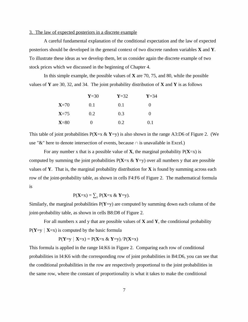
3. The law of expected posteriors in a discrete example

A careful fundamental explanation of the conditional expectation and the law of expected

posteriors should be developed in the general context of two discrete random variables X and Y.

To illustrate these ideas as we develop them, let us consider again the discrete example of two

stock prices which we discussed in the beginning of Chapter 4.

In this simple example, the possible values of X are 70, 75, and 80, while the possible

values of Y are 30, 32, and 34. The joint probability distribution of X and Y is as follows

Y=30 Y=32 Y=34

X=70 0.1 0.1 0

X=75 0.2 0.3 0

X=80 0 0.2 0.1

This table of joint probabilities P(X=x & Y=y) is also shown in the range A3:D6 of Figure 2. (We

use "&" here to denote intersection of events, because 1 is unavailable in Excel.)

For any number x that is a possible value of X, the marginal probability P(X=x) is

computed by summing the joint probabilities P(X=x & Y=y) over all numbers y that are possible

values of Y. That is, the marginal probability distribution for X is found by summing across each

row of the joint-probability table, as shown in cells F4:F6 of Figure 2. The mathematical formula

is

P(X=x) = 3 P(X=x & Y=y).y

Similarly, the marginal probabilities P(Y=y) are computed by summing down each column of the

joint­probability table, as shown in cells B8:D8 of Figure 2.

For all numbers x and y that are possible values of X and Y, the conditional probability

P(Y=y * X=x) is computed by the basic formula

P(Y=y * X=x) = P(X=x & Y=y)'P(X=x)

This formula is applied in the range I4:K6 in Figure 2. Comparing each row of conditional

probabilities in I4:K6 with the corresponding row of joint probabilities in B4:D6, you can see that

the conditional probabilities in the row are respectively proportional to the joint probabilities in

the same row, where the constant of proportionality is what it takes to make the conditional

8

probabilities sum to 1 across the row. For example, the top row of conditional probabilities given

X=70 in I4:K4

P(Y=30*X=70) = 0.5, P(Y=32*X=70) = 0.5, P(Y=34*X=70) = 0,

which are proportional to the corresponding joint probabilities (0.1, 0.1, 0) in B4:D4.

If we learned that the value of X was some particular number x, then our conditionally

expected value of Y given that X=x would be

E(Y * X=x) = 3 P(Y=y * X=x) * yy

where the summation is over all number y that are possible values of Y. In our example, the

conditionally expected value of Y given X=70 is

E(Y * X =70) = 0.5*30 + 0.5*32 + 0 * 34 = 31.00

Similarly, the conditionally expected value of Y given X=75 in this example is

E(Y * X =75) = 0.4*30 + 0.6*32 + 0 * 34 = 31.20

The conditionally expected value of Y given X=80 is

E(Y * X =80) = 0*30 +0.667*32 + 0.333*34 = 32.67

These conditionally expected values are computed by SUMPRODUCT formulas in cells M4:M6

in Figure 2. If we are about to learn X but not Y, then our posterior expected value of Y after

learning X will be either 31.00 or 31.20 or 32.67, depending on whether X turns out to be 70, 75,

or 80. These three possible value of X have prior probability 0.2, 0.5, and 0.3 respectively. So

our prior expected value of the posterior expected value of Y that we will apply after learning X is

E(E(Y*X)) = 0.2*31.00 + 0.5*31.20 + 0.3*32.67 = 31.6

as shown in cell M9 of Figure 2. But before learning X, our expected value of Y is the same

number, as shown in cell C11 of Figure 2:

E(Y) = 0.3 *30 + 0.6*32 + 0.1*34 = 31.6

More generally, the law of expected posteriors says that, before we observe any random

variable X, our expected value of another random variable Y must be equal to the expected value

of what we will think is the expected value of Y after we observe X. The formula for the

expected posterior law is be written:

E(Y) = 3 P(X=x) * E(Y* X=x).x

(Here the summation is over all x that are possible values of X.) Or, as we may write this formula

9

more briefly as

E(Y) = E(E(Y*X))

which may be briefly summarized as "the expected value of the expected value is equal to the

expected value."

If you would like a proof of this law of expected posteriors, it can be proven as follows

(using the basic formula for conditional probabilities at the third step):

3 P(X=x) * E(Y*X=x) = 3 P(X=x) * 3 P(Y=y*X=y) * yx x y

= 3 3 P(X=x) * P(Y=y * X=x) * yx y

= 3 3 P(X=x & Y=y) * yx y

= 3 P(Y=y) * y = E(Y).y

As another application of this expected-posterior law, let A denote any event, and define

W to be a random variable such that W = 1 if the event A is true, but W = 0 if the event A is

false. Then

E(W) = P(A) * 1 + (1 ! P(A)) * 0 = P(A).

That is, the expected value of this random variable W is equal to the probability of the event A.

Now suppose that X is any other random variable such that observing the value of X might cause

us to revise our beliefs about the probability of A. Then the conditionally expected value of W

given the value of X would be similarly equal to the conditional probability of A given the value of

X. That is, for any number x that is a possible value of the random variable X,

E(W* X=x) = P(A* X=x).

Thus, the general equation

E(W) = 3 P(X=x) * E(W* X=x)x

gives us the following probability equation:

P(A) = 3 P(X=x) * P(A* X=x)x

which may be written more briefly as P(A) = E(P(A*X)). This equation says that the probability

of A, as we assess it given our current information, must equal the current expected value of what

we would think is probability of A after learning the value of X. Learning X might cause us to

revise our assessment of the probability of A upwards or downwards, but the weighted average of

these possible revisions, weighted by their likelihoods, must be equal to our currently assessed

10

probability P(A).

In our example, let A denote the event that Y=32. So before X is learned, the prior

probability of A is

P(A) = P(Y=32) = 0.6,

as shown in cell C8 of Figure 2. Then the posterior probability of A given the value of X would

be either 0.5 or 0.6 or 0.667, depending on whether X is 70 or 75 or 80, as shown in cells J4:J6.

But the respective probabilities of these three values of X are 0.2, 0.5, and 0.3, as shown in cells

F4:F6. So before we learn X, our prior expected value of the posterior probability of A given X

is

E(P(A*X)) = 0.2*0.5 + 0.5*0.6 + 0.3*0.667 = 0.6

as shown in cell J11.

The idea of posterior conditional probabilities as random variables is applied to build a

simulation model of X and Y for this example in row 15 of Figure 2. The random variable X is

simulated straightforwardly in cell B15 by the formula

=DISCRINV(RAND(),A4:A6,F4:F6)

using the list of possible values of X in A4:A6 and the corresponding marginal probabilities

in F4:F6. But if we similarly simulated Y using its marginal probabilities and a different RAND

then we would have a pair of independent random variables. So the trick is first to compute the

posterior conditional probability distribution for Y given X that would apply with the simulated

value of X. These conditional probabilities are computed by in cells I15:J15 by entering

=LOOKUP($B$15, $H$4:$H$6, I4:I6)

into cell I15 and then copying I15 to I15:K15. This LOOKUP formula in cell I15 looks in the

range H4:H6 for a cell that matches the simulated value of X in cell B15, and then it returns the

corresponding conditional probability that it finds in the same row of I4:I6. So cells I15:K15

always contain the appropriate conditional probability distribution for Y given that X is equal to

the value in cell B15. Thus, we can simulate Y in cell C15 by the formula

=DISCRINV(RAND(),I14:K14,I15:K15)

(where I14:K14 contains the list of possible values of Y). So the formulaic dependence of C15 on

B15 (indirectly via I15:K15) has been constructed to give us the required statistical dependence to

11

jointly simulate X and Y in this example.

An important warning must be given about the use of the function LOOKUP. In the

formula

LOOKUP(B15,H4:H6,I4:I6)

LOOKUP starts searching at the top of the H4:H6, looking for a cell that matches the value of

cell B15. But as it searches downwards in H4:H6, if it first finds a cell that has a value greater

than B15, then it will stop searching and take the previous cell as its best match (even if an exact

match existed lower down in the range H4:H6). Thus, it is essential that the values in LOOKUP's

search range (its second parameter) must be sorted in ascending order. (You can use

Data>Sort>Ascending on the search range if necessary.)

This model of (X,Y) in cells B15:C15 here may be contrasted with the simulation model

that we constructed in cells I26:J26 in Figure 2 of Chapter 4, where neither cell was formulaically

dependent on the other, and so statistical dependence had to be created by using the same RAND

(in I24) for both random variables. But the joint probability distribution of cells I26:J26 in Figure

2 of Chapter 4 is exactly the same as joint probability distribution of cells B15:C15 in Figure 2

here. No statistical test could ever distinguish one pair's simulation data from the other pair's.

The lower portion of Figure 2 here contains an analysis of simulation data from the model

in cells B15:C15 here, to illustrate how the law of expected posteriors holds true also for

estimates of conditional expectations and conditional probabilities that are computed from

simulation data. In cells K20:K22, conditional expectations of Y given each possible value of X

are estimated from the simulation data. In cells J20:J22, the corresponding prior probabilities of

these possible values of X are also estimated from the data. Then cell K25 estimates the expected

value of the posterior conditional expectation of Y given X. Note that K25 returns the same

value as K28, which directly estimates E(Y) from the simulation data. Similarly, the conditional

probabilities of A given each possible value of X are estimated in L20:L22. Then cell L25

estimates the expected value of the posterior conditional probability of A given X. Note that L25

returns the same value as L28, which directly estimates P(A) from the simulation data.

12345678910111213141516171819202122232425262728293031323334353637383940414243444546474849505152

A B C D E F G H I J K L MJointProbys P(X=x&Y=y) CondlProbys P(Y=y|X=x)

y= y=x= \ 30 32 34 P(X=x) x= \ 30 32 34 E(Y|X=x)

70 0.1 0.1 0 0.2 70 0.5 0.5 0 3175 0.2 0.3 0 0.5 75 0.4 0.6 0 31.280 0 0.2 0.1 0.3 80 0 0.666667 0.333333 32.67

P(Y=y)0.3 0.6 0.1

Let A denote the event that Y=32.E(X) E(Y) E(P(A|X)) E(E(Y|X))75.5 31.6 0.6 31.6

SIMULATION MODEL y=X Y 30 32 3480 34 P(Y=y|X) 0 0.666667 0.333333

X Y A With X= 70SimTable80 34 0 Y A Estimates from simulation

0 80 32 1 .. .. x P(X=x) E(Y|X=x) P(A|X=x)0.01 75 32 1 .. .. 70 0.267 31.037 0.5190.02 70 30 0 30 0 75 0.455 31.130 0.5650.03 75 32 1 .. .. 80 0.277 32.643 0.6790.04 75 30 0 .. ..0.05 75 30 0 .. .. E(E(Y|X)) E(P(A|X))0.06 75 30 0 .. .. 31.52475 0.5840.07 70 32 1 32 10.08 75 32 1 .. .. E(Y) P(A)0.09 75 32 1 .. .. 31.52475 0.5840.1 70 30 0 30 0 FORMULAS

0.11 70 32 1 32 1 F4. =SUM(B4:D4) F4 copied to F4:F60.12 80 32 1 .. .. I4. =B4/$F4 I4 copied to I4:K60.13 75 32 1 .. .. M4. =SUMPRODUCT(I4:K4,$B$3:$D$3)0.14 70 32 1 32 1 M4 copied to M4:M60.15 80 34 0 .. .. B8. =SUM(B4:B6) B8 copied to B8:D80.16 70 32 1 32 1 B11. =SUMPRODUCT(A4:A6,F4:F6)0.17 75 30 0 .. .. C11. =SUMPRODUCT(B3:D3,B8:D8)0.18 75 32 1 .. .. J11. =SUMPRODUCT(J4:J6,$F$4:$F$6)0.19 75 32 1 .. .. M11. =SUMPRODUCT(M4:M6,$F$4:$F$6)0.2 70 30 0 30 0 B15. =DISCRINV(RAND(),A4:A6,F4:F6)

0.21 70 32 1 32 1 I15. =LOOKUP($B$15,$H$4:$H$6,I4:I6)0.22 70 32 1 32 1 I15 copied to I15:K150.23 75 32 1 .. .. C15. =DISCRINV(RAND(),I14:K14,I15:K15)0.24 75 32 1 .. .. B18. =B15 C18. =C150.25 70 32 1 32 1 D18. =IF(C18=32,1,0)0.26 80 34 0 .. .. F19. =IF($B19=$H$17,C19,"..")0.27 70 32 1 32 1 F19 copied to F19:G1190.28 75 32 1 .. .. J20. =COUNT(F19:F119)/COUNT(C19:C119)0.29 75 32 1 .. .. K20. =AVERAGE(F19:F119) K20 copied to L200.3 80 34 0 .. .. J21:L22. {=TABLE(,H17)}

0.31 70 32 1 32 1 K25. =SUMPRODUCT(K20:K22,$J$20:$J$22)0.32 80 34 0 .. .. L25. =SUMPRODUCT(L20:L22,$J$20:$J$22)0.33 80 32 1 .. .. K28. =AVERAGE(C19:C119) K28 copied to L28

12

Figure 2.

13

4. Linear regression models

We now consider a special form of formulaic dependence among random variables that is

probably assumed by statisticians more often than any other: the linear regression model. In a

linear regression model, a random variable Y is made dependent on other random variables

(X ,...,X ) by assuming that Y is a linear function of these other random variables (X ,...,X ) plus1 K 1 K

a Normal error term. A Normal error term is a Normal random variable that has mean 0 and is

independent of the values of the other random variables (X ,...,X ). To define such a linear1 K

regression model where Y depends on K other random variables, we must specify K+2 constant

parameters: the coefficients for each of the K explanatory random variables in the linear function,

the Y-axis intercept of the linear function, and the standard deviation of the Normal error term.

An example of a linear regression model is shown in Figure 3, where a random variable Y

in cell B12 is made to depend on another random variable X in cell A12. The value 3 in cell B4 is

the coefficient of X in the linear function, the value !10 in cell B6 is the Y-axis intercept of the

linear function, and the value 8 in cell B8 is the standard deviation of the Normal error term. So

with these parameters in cells B4, B6, and B8, the formula for Y in cell B12 is

=$B$6+$B$4*A12+NORMINV(RAND(),0,$B$8)

The value of the X in cell A12 here is generated by a similar formula

=$A$4+NORMINV(RAND(),0,$A$6)

where cell A4 contains the value 10 and cell A6 contains the value 2. That is, the random variable

X here has no random precedents, and it is simply the constant 10 plus a Normal error term with

standard deviation 2.

But adding a constant to a Normal random variable yields a Normal random variable with

mean increased by the amount of this constant. So X in cell A12 is a Normal random variable

with mean 10 and standard deviation 2, and the formula in cell A12 is completely equivalent to

=NORMINV(RAND(),$A$4,$A$6)

Similarly, the formula for Y in cell B12 could have been written equivalently as

=NORMINV(RAND(),$B$6+$B$4*A12,$B$8)

which is shorter but harder to read.

12345678910111213141516171819202122232425262728293031

A B C D E F G HParameters: Computed from parameters:for X for Y given X E(Y) Covar(X,Y)E(X) X coefficient 20 12

10 3 Stdev(Y) Correl(X,Y) CorandsStdev(X) Intercept 10 0.6 0.0788 0.3993

2 -10 X YStd error 7.17 17.45

8

Data: Computed from data:X Y Estimates for X Estimates for Y given X11.39 25.27 E(X) Regressn Array ... 7 Rows x 1 Columns8.90 12.86 10.309 X(1) Coefficient6.06 12.19 Stdev(X) 3.4249.83 29.13 2.370 Intercept11.85 42.34 -14.3199.44 9.59 Std Error11.11 20.04 FORMULAS 9.0548.35 29.52 A12. =$A$4+NORMINV(RAND(),0,$A$6)11.31 33.69 B12. =$B$6+$B$4*A12+NORMINV(RAND(),0,$B$8)6.44 7.98 A12:B12 copied to A12:B3110.06 12.68 E13. =AVERAGE(A12:A31)11.00 26.90 E15. =STDEV(A12:A31)8.96 7.82 F12:F18. {=REGRESSN(A12:A31,B12:B31)}12.66 18.17 E3. =B6+B4*A414.36 31.41 F3. =B4*A6^28.72 20.13 E5. =((A6*B4)^2+B8^2)^0.511.28 17.17 F5. =F3/(A6*E5)11.58 30.44 G5:H5. {=CORAND(F5)}15.30 38.03 G7. =NORMINV(G5,A4,A6)7.57 -5.84 H7. =NORMINV(H5,E3,E5)

14

Figure 3.

The formulas from A12:B12 in Figure 3 have been copied to fill the range A12:B31 with

20 independent pairs that have the same joint distribution. That is, in each row from 13 to 31, the

cells in the A and B column are drawn from the same joint distribution as X and Y in A12:B12.

In each of these rows, the value of the B-cell depends on the value of the A-cell according to the

linear regression relationship specified by the parameters in $B$3:$B$8, but the values in each

row are independent of the values in all other rows.

15

The fundamental problem of statistical regression analysis is to look at statistical data like

the 20 pairs in A12:B31, and guess the linear regression relationship that underlies the data.

Excel offers several different ways of doing statistical regression analysis. In particular, with the

Excel's Analysis ToolPak added in, you should try using the menu command sequence

Tools>DataAnalysis>Regression. But for a first illustration of regression analysis, Figure 3 uses a

simple regression-analysis function called REGRESSN that is added by Simtools.

The REGRESSN function has two parameters: the XDataRange first, and the

YDataRange second. The YDataRange should be a range of cells in one column that contain the

sample data for the dependent random variable Y. When Y is dependent on K explanatory

variables in the regression, the XDataRange will be a range with K columns, one for each and as

many rows as the YDataRange. When there are K explanatory variables, the REGRESSN

function should be entered as an array function filling 7 rows by K columns, where it will return

its best estimate of the regression relationship between the dependent variable and the K

explanatory variables. In this example, our random variable Y is dependent on just one

explanatory variable X, and so we have K=1. The XDataRange is A12:A31, the YDataRange is

B12:B31, and the array formula

{=REGRESSN(A12:A31,B12:B31)}

has been entered into the seven cells F12:F18 to display the estimated regression parameters: the

coefficient of X in the regression, the Y-axis intercept, and the standard deviation of the Normal

error term, which may also be called the standard error of the regression.

If you try recalculating the spreadsheet in Figure 3, so that the simulated X and Y data is

regenerated in cells A12:B31, you will see the regression estimates in F12:F18 varying around the

true underlying parameters that we can see in B3:B8. More sophisticated regression-analysis

software (such as that in Excel's Analysis ToolPak) will generate 95% confidence intervals for the

regression parameters around these estimates.

Regression analysis in F12:F18 here only assesses the parameters of the conditional

probability distribution of Y given X. So to complete our estimation of the joint distribution of X

and Y, we need to estimate the parameters of the marginal probability distribution of X. If we

know that X is drawn from a Normal probability distribution but we do not know its mean and

16

standard deviation, then we can use the sample average and the sample standard deviation of our

X data (as shown in cells E13 and E15 of Figure 3) to estimate the mean and standard deviation

parameters of the Normal distribution that generated our X data.

Statistical regression analysis in general does not require any specific assumptions about

the probability distributions that generated the explanatory X data. But if the explanatory X is a

Normal random variable (or, when K > 1, if the explanatory X variables are Multivariate Normal),

then the joint distribution of X and Y together is Multivariate Normal. Thus our X and Y random

variables in A12:B12, for example, are Multivariate Normal random variables, just like the

random variables that we generated in Chapter 4 with CORANDs driving the NORMINVs.

The difference between the treatment of Multivariate Normals here and in Chapter 4 is the

parametric form that we use to characterize these Multivariate Normal random variables. Here

the parameters are the mean E(X) and standard deviation Stdev(X), which characterize the

marginal distribution of X, and the Intercept, Coefficient, and StdError parameters of the

regression relationship

Y = Intercept + Coefficient * X +NORMINV(RAND(),0,StdError)

which characterize the conditional distribution of Y given X. But in Chapter 4 we parameterized

the Multivariate Normal random variables by their individual means and standard deviations and

their pairwise correlations. In cases like this, where we have only one explanatory variable X in

the regression model, the other parameters of the Multivariate-Normal distribution of X and Y

can be computed from the regression parameters by the equations:

E(Y) = Intercept + Coefficient * E(X)

Stdev(Y) = ((Coefficient) * Stdev(X))^2 + StdError^2)^0.5

Correl(X,Y) = (Coefficient) * Stdev(X)'Stdev(Y)

(These equations can be derived from equations (3) through (6) in Chapter 4.) These equations

are applied to compute these parameters in E2:F5 of Figure 3. These computed parameters are

then used with CORAND (in G5:H5) to make a simulation of X and Y in cells G7:H7 that is

completely equivalent to the simulation that we made with regression in cells A12:B12. That is,

no statistical test could distinguish between data taken from cells A12:B12 and data taken from

cells G7:H7.

17

Notice that the standard deviation of Y, as computed in cell E5 of Figure 3, is larger than

the standard error of the regression, which has been given in cell B8 (10 > 8). The standard error

of the regression is the conditional standard deviation of Y given X. Recall (as we saw in the

comparison of cell B12 with cells J15:J36 in Figure 1) that such a conditional standard deviation

should be generally smaller than the unconditional standard deviation, because the standard

deviation is a measure of uncertainty and learning X tends to reduce our uncertainty about the

dependent variable Y.

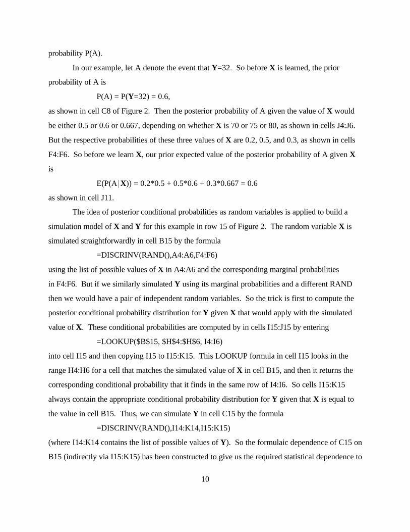
4. Regression analysis and least squared errors

Regression analysis is a powerful statistical method that you should study in detail in

another course. But I can tell you here a bit more about how the estimates of a statistical

regression analysis are determined from the data. Consider again the annual growth ratio data for

Funds 1 and 2 shown in cells B2:C11 of Figure 4, and let us try to estimate a regression model in

which the growth ratio of Fund 2 depends on the growth ratio of Fund 1 in each year.

We start by searching for a linear function that can be used to predict the growth ratio of

Fund 2 as a function of the growth ratio of Fund 1. In Figure 4, the values of cells A14 and B14

will be interpreted as the intercept and coefficient of this linear function. Then, based on the 1980

growth ratio of Fund 1 in cell B2, our linear estimate of estimate of Fund 2's growth ratio in 1980

can be computed by the formula

=$A$14+$B$14*B2

which has been entered into cell D2. Then copying cell D2 to D2:D11 gives us a column of linear

estimates of Fund 2's growth based only on the growth of Fund 1 in the same year.

The numerical value of these estimates will depend, of course, on the intercept and

coefficient that we have entered into cells A14 and B14. For example, if we enter the value 0 into

cell A14 and the value 1 into cell B14, then our linear estimate of Fund 2's growth will be just the

same as Fund 1's growth for each year. Unfortunately, no matter what intercept and coefficient

we may try, our linear estimates in D2:D11 will be wrong (different from C2:C11) in most or all

the years for which we have data. But we can at least ask for an intercept and coefficient that will

generate linear estimates that have the smallest overall errors, in some sense.

18

The overall measure of our errors that statisticians use in regression analysis is an adjusted

average the squared errors of our linear estimates. The squared error of the linear estimate in

1980 is computed in cell E2 of Figure 4 by the formula

=(D2!C2)^2

and this formula in E2 has then been copied to E2:E11. The adjusted average squared error is

computed in cell E14 by the formula

=SUM(E2:E11)'(COUNT(E2:E11)!COUNT(A14:B14))

That is, the adjusted average differs from the true average in that we divide, not by the number of

data points, but by the number of data points minus the number of linear parameters that are we

have to find in the linear function. This denominator (number of data points minus number of

parameters in the linear function) is called the degrees of freedom in the regression.

Now let us ask Solver to minimize this adjusted average squared error in cell E14 by

changing the parameters of the linear function in cells A14:B14. The resulting optimal solution

that Solver returns for this optimization problem is shown in cells A14:B14 of Figure 4 (an

intercept of !0.1311 and a coefficient of 1.1305). That this optimal solution is the same as the

intercept and coefficient that the REGRESSN function returns in cells A21 and A19 for this data,

because statistical regression analysis is designed to find the linear function that minimizes the

adjusted average squared error in this sense.

Cell E16 in Figure 4 computes that square root of the adjusted average squared error, with

the formula

=E14^0.5

Notice that the result of this formula in cell E16 is the same as the standard error of the regression

is that REGRESSN returns in cell A23 (0.0915). That is, the estimated standard error of the

regression (or the estimated standard deviation of the Normal error term in the regression model)

is the square root of the minimal adjusted-average squared error.

12345678910111213141516171819202122232425262728293031323334353637383940414243444546474849

A B C D E F GFund 1 Fund 2 Linear estimate of 2 Squared error

1980 1.22 1.28 1.2427 0.001411981 1.09 1.20 1.0962 0.010361982 0.92 0.83 0.9033 0.005091983 1.37 1.48 1.4226 0.003211984 1.01 0.96 1.0053 0.002211985 1.15 1.22 1.1645 0.002631986 1.26 1.15 1.2921 0.019821987 1.25 1.17 1.2856 0.013091988 0.93 0.96 0.9163 0.001531989 1.19 1.31 1.2198 0.00759

Intercept Coefficient Adjusted avg sq err-0.1311 1.1305 0.00837

SOLVER: minimize E14 by changing A14:B14 Std err0.0915

Regressn Array ... 7 Rows x 1 ColumnsX(1) Coefficient Fund 1 Fund 2

1.1305 Simulation model 0.991 0.964Intercept

-0.1311 FORMULASStd Error D2. =$A$14+$B$14*B2 D2 copied to D2:D11

0.0915 E2. =(D2-C2)^2 E2 copied to E2:E11E14. =SUM(E2:E11)/(COUNT(E2:E11)-COUNT(A14:B14))E16. =E14^0.5A17:A23. {=REGRESSN(B2:B11,C2:C11)}E19. =NORMINV(RAND(),AVERAGE(B2:B11),STDEV(B2:B11))F19. =A21+A19*E19+NORMINV(RAND(),0,A23)B33. =E19C33. =F19

Fund 1 (X)Fund 2SimTable 0.991 0.964

0 1.2264 1.2237 0.47 0.4002240.005 1.1678 1.0853 1.7 1.7906950.01 1.0226 1.0947

0.015 1.0548 1.04510.02 0.9151 0.8193

0.025 1.4021 1.65610.03 0.8927 1.0064

0.035 0.8644 0.82580.04 1.2598 1.1832

0.045 1.1135 1.22220.05 1.0394 1.2006

0.055 1.2948 1.43270.06 0.8942 0.7007

0.065 1.2975 1.30320.07 1.0191 0.9709

0.075 0.8652 0.8862

0.40

0.60

0.80

1.00

1.20

1.40

1.60

1.80

0.40 0.60 0.80 1.00 1.20 1.40 1.60 1.80Fund 1 annual growth ratios

Fund

2 a

nnua

l gro

wth

rat

ios

19

Figure 4.

20

If we had used the simple average in cell E14 (dividing by the number of data points,

instead of dividing by the number of degrees of freedom) then Solver would have still given us the

same optimal intercept and coefficient in A14:B14 when we asked it to minimize E14. But the

square root of the average squared error would have been slightly smaller. Regression analysis

uses this adjusted average squared error (dividing by the number of degrees of freedom) because

otherwise our ability to adjust these linear parameters to fit our data would bias downwards our

estimate of the variance of the Normal errors in the regression.

In cells E19:F19 of Figure 4, this statistically estimated regression model is applied to

make a simulation model for forecasting the growth ratios of Funds 1 and 2 in future years. The

growth ratio of Fund 1 is simulated in cell E19 by the formula

=NORMINV(RAND(),AVERAGE(B2:B11),STDEV(B2:B11))

Then the growth ratio of Fund 2 is simulated in cell F19 by the formula

=A21+A19*E19+NORMINV(RAND(),0,A23)

using the intercept, coefficient, and standard error from the REGRESSN array. A simulation

table containing 200 independent recalculations of cells E19:F19 has been made in this

spreadsheet and the results are shown in the scatter chart in the lower right of Figure 4. The

optimal linear function for estimating Fund 2 from Fund 1 is also shown by a dashed line in that

chart.

The scatter plot generated by our regression model in Figure 4 here should look very

similar to the right-hand scatter plot in Figure 6 of Chapter 4, which shows 200 simulations that

were generated from a CORAND model that we fit to the same historical data. There is actually

a very small difference between the Multivariate Normal probability distributions that generated

these two scatter plots. The difference is caused by the practice of dividing by the number of

degrees of freedom to estimate the standard error in a regression analysis, instead of dividing by

the sample size minus 1 as we do in calculating sample standard deviations. (The problem is that

the regression-analysis formulas have been designed to yield unbiased estimates of the conditional

variance of the dependent variable given the explanatory variables, whereas the sample standard-

deviation formula has been designed to yield unbiased estimates of the unconditional variance.)

The result is that Fund 2's growth ratios have a slightly higher standard deviation in the regression

21

model here than in the CORAND model of Chapter 4. But this difference is small, and it vanishes

when the number of data points is large.

Conditional expectation problems:

1. A construction project has two stages. Let X denote the cost of the first stage and let Y

denote the cost of the second stage (both in thousands of dollars). Suppose that the joint

distribution of these costs is as follows:

Y = 200 Y = 250 Y = 300

X = 90 0 .15 .15

X = 70 .10 .20 .16

X = 50 .09 .09 .06

(a) Compute the expected value of Y.

(b) Compute the conditionally expected value of Y given each of the possible values of X.

(c) Show that the formula

E(Y) = 3 P(X=m) ( E(Y* X=m)m

is satisfied for this example.

(d) If you learned that X > 60 (that is, X may equal 70 or 90, but not 50), then what would be

your conditionally expected value of Y given this new information?

(Hint: if you have difficulty with (d), try first to compute

P(Y=200* X>60), P(Y=250* X>60), and P(Y=300* X>60).)

2. A and B are unknown quantities. Given my current information only, I think that

E(A) = 3000. But if I knew the value of B, I would revise my beliefs about A to

E(A|B=0) = 1000 or E(A|B=1) = 9000. If B can only equal 0 or 1, what is P(B=0)?