Embed Size (px)
Citation preview

University of Tennessee, Knoxville University of Tennessee, Knoxville
TRACE: Tennessee Research and Creative TRACE: Tennessee Research and Creative
Exchange Exchange
Masters Theses Graduate School
5-2017
Practical Methods for Optimizing Equipment Maintenance Practical Methods for Optimizing Equipment Maintenance
Strategies Using an Analytic Hierarchy Process and Prognostic Strategies Using an Analytic Hierarchy Process and Prognostic
Algorithms Algorithms
Gregory Michael Bosco University of Tennessee, Knoxville, [email protected]
Follow this and additional works at: https://trace.tennessee.edu/utk_gradthes
Part of the Nuclear Engineering Commons
Recommended Citation Recommended Citation Bosco, Gregory Michael, "Practical Methods for Optimizing Equipment Maintenance Strategies Using an Analytic Hierarchy Process and Prognostic Algorithms. " Master's Thesis, University of Tennessee, 2017. https://trace.tennessee.edu/utk_gradthes/4726
This Thesis is brought to you for free and open access by the Graduate School at TRACE: Tennessee Research and Creative Exchange. It has been accepted for inclusion in Masters Theses by an authorized administrator of TRACE: Tennessee Research and Creative Exchange. For more information, please contact [email protected].

To the Graduate Council:
I am submitting herewith a thesis written by Gregory Michael Bosco entitled "Practical Methods
for Optimizing Equipment Maintenance Strategies Using an Analytic Hierarchy Process and
Prognostic Algorithms." I have examined the final electronic copy of this thesis for form and
content and recommend that it be accepted in partial fulfillment of the requirements for the
degree of Master of Science, with a major in Nuclear Engineering.
Jamie B. Coble, Major Professor
We have read this thesis and recommend its acceptance:
Belle Upadhyaya, Mingzhou Jin
Accepted for the Council:
Dixie L. Thompson
Vice Provost and Dean of the Graduate School
(Original signatures are on file with official student records.)

Practical Methods for Optimizing
Equipment Maintenance Strategies
Using an Analytic Hierarchy Process and
Prognostic Algorithms
A Thesis Presented for the
Master of Science
Degree
The University of Tennessee, Knoxville
Gregory Michael Bosco
May 2017

ii
Copyright © 2017 by Gregory M. Bosco
All rights reserved.

iii
DEDICATION
To almighty God and my savior, Jesus Christ: I dedicate myself to doing your will
by applying this knowledge to promote safe and responsible equipment
operations.
To my daughters: I think we live in a time when young girls like you are limited
only by their imagination and dedication to achieving their dreams. Your dreams
will not come easily, though. You will need to sacrifice, sometimes putting aside
important parts of your life to focus on the job ahead. You should expect
setbacks and failures. When they happen, pick yourself up, make adjustments
and move forward – always forward. You should expect criticism, doubters, and
roadblocks; some of them will be unfair and beyond control. If you cannot work
through them, go around. So make a habit of turning disappointment into
motivation. You will also have successes, often creating a difference between
you and other people. Be humble and give back; help people achieve their
potential just like so many have done for you. Most important, believe in
yourself. I dedicate this thesis and the time spent working towards it to you.

iv
ACKNOWLEDGEMENTS
To Dr. Jamie Coble, my advisor and review committee chair from the Department
of Nuclear Engineering at the University of Tennessee: Thank you for sharing
your knowledge and insight, and helping me find the answers to my questions
over the past few years. You made a difference.
To Dr. Jin and Dr. Upadhyaya, University of Tennessee professors and members
of my thesis review committee: Thank you for your time and helpful feedback.
The UTK R&M curriculum you helped develop is important, relevant, progressive,
and perhaps most meaningful – interesting.
To my wife - thank you. I could not have done this without you.

v
ABSTRACT
Many large organizations report limited success using Condition Based
Maintenance (CbM). This work explains some of the causes for limited success,
and recommends practical methods that enable the benefits of CbM. The
backbone of CbM is a Prognostics and Health Management (PHM) system. Use
of PHM alone does not ensure success; it needs to be integrated into enterprise
level processes and culture, and aligned with customer expectations. To
integrate PHM, this work recommends a novel life cycle framework, expanding
the concept of maintenance into several levels beginning with an overarching
maintenance strategy and subordinate policies, tactics, and PHM analytical
methods. During the design and in-service phases of the equipment’s life, an
organization must prove that a maintenance policy satisfies specific safety and
technical requirements, business practices, and is supported by the logistic and
resourcing plan to satisfy end-user needs and expectations. These factors often
compete with each other because they are designed and considered separately,
and serve disparate customers. This work recommends using the Analytic
Hierarchy Process (AHP) as a practical method for consolidating input from
stakeholders and quantifying the most preferred maintenance policy. AHP forces
simultaneous consideration of all factors, resolving conflicts in the trade-space of
the decision process. When used within the recommended life cycle framework,
it is a vehicle for justifying the decision to transition from generalized high-level
concepts down to specific lower-level actions. This work demonstrates AHP
using degradation data, prognostic algorithms, cost data, and stakeholder input
to select the most preferred maintenance policy for a paint coating system. It
concludes the following for this particular system: A proactive maintenance
policy is most preferred, and a predictive (CbM) policy is more preferred than
predeterminative (time-directed) and corrective policies. A General Path
prognostic Model with Bayesian updating (GPM) provides the most accurate
prediction of the Remaining Useful Life (RUL). Long periods between

vi
inspections and use of categorical variables in inspection reports severely limit
the accuracy in predicting the RUL. In summary, this work recommends using
the proposed life cycle model, AHP, PHM, a GPM model, and embedded
sensors to improve the success of a CbM policy.

vii
TABLE OF CONTENTS
Chapter 1: Introduction ........................................................................................ 1
1.1 Problem, Purpose, Goal, and Motivation ................................................... 1
1.2 Organization of Paper ................................................................................ 3
1.3 Additional Considerations .......................................................................... 7
Chapter 2: Literature Review ............................................................................. 10
2.1 (Levels 0 & 1) Equipment Life Cycle & Stages ....................................... 10
2.2 (Levels 2 & 3) Maintenance & Strategies ................................................ 12
2.3 (Level 4) Maintenance Policies ............................................................... 14
2.4 (Level 5) Maintenance Tactics ................................................................ 18
2.5 (Linking Levels 1 - 5 to Levels 6 - 8) Optimizing Maintenance ................ 24
2.6 (Levels 6 & 7) Prognostics and Health Management .............................. 51
2.7 (Level 8) Data / Knowledge Feedback & Implementation ....................... 77
Chapter 3: Materials and Methods ..................................................................... 78
3.1 (Levels 0 – 5) AHP .................................................................................. 78
3.2 (Level 6) Data Management ................................................................... 83
3.3 (Level 7) Prognostic Methods ................................................................. 89
3.4 Cost Considerations ............................................................................... 108
Chapter 4: Results and Discussion .................................................................. 110
4.1 (Levels 0 - 5) AHP Models .................................................................... 110
4.2 (Level 7) Prognostic Methods (Models) ................................................ 114
Chapter 5: Conclusions and Recommendations .............................................. 127
Chapter 6: Future Work ................................................................................... 131
List of References ............................................................................................. 133
Appendices ....................................................................................................... 144
Appendix A - Tables .......................................................................................... 145
Appendix B - Figures ........................................................................................ 159
Vita .................................................................................................................... 169

viii
LIST OF TABLES Table 1. Continuous Distributions and Parameters ............................................ 90
Table 2. Maintenance Policy Costs .................................................................. 108
Table 3. Critical Criteria Analysis ..................................................................... 114
Table 4. Benefit-Cost Ratio .............................................................................. 114
Table 5. Type 1 Models – Fitted Functions & Parameter Results .................... 115
Table 6. Type 1 Models – Function Goodness of Fit Results ........................... 116
Table 7. Cox PhM Statistics ............................................................................. 118
Table 8. Type 3 Models – GPM with Bayesian Mean Squared Error ............... 121
Table 9. Quadratic Model Parameter Evaluation ............................................. 122
Table 10. Cumulative Relative Accuracy of Prognostic Models ....................... 125
Table 11. Literature Review of Topics .............................................................. 145
Table 12. Literature Review of Topic Publishing By Year ................................ 146
Table 13. Literature Review, Quantity of Publishing By Year ........................... 147
Table 14. Literature Review on Optimization Criteria Reported ....................... 149
Table 15. Literature Review on Optimization Case Studies Categories ........... 150
Table 16. Literature Review on Optimization Case Studies ............................. 151
Table 17. PCA and PLS Applications for Fault Diagnostics ............................. 152
Table 18. AHP Demonstration – Requirements Definition ............................... 153
Table 19. AHP Demonstration – Judgement Score Matrix ............................... 155
Table 20. AHP Demonstration – Level 1 Criteria PCM .................................... 156
Table 21. AHP Demonstration – Level 2 & Level 3 Criteria PCM .................... 157
Table 22. Database Structure .......................................................................... 158

ix
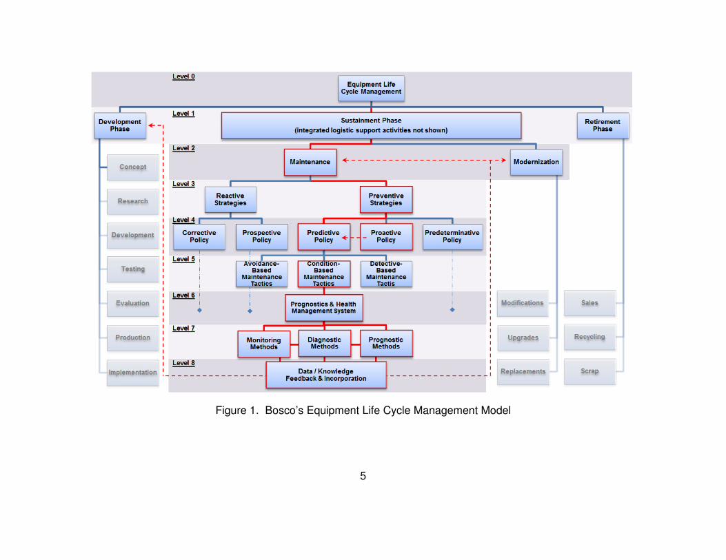
LIST OF FIGURES Figure 1. Bosco’s Equipment Life Cycle Management Model .............................. 5
Figure 2. AHP in Maintenance Policy Decision .................................................... 6
Figure 3. Life Cycle Stage Comparison ............................................................. 11
Figure 4. Affordable System Operational Effectiveness, [32] ............................. 27
Figure 5. Affordable Solutions – Trade Space [36] ............................................ 28
Figure 6. Optimal Cost Effective Time to Replace ............................................. 30
Figure 7. Elements of Maintenance Downtime [2].............................................. 34
Figure 8. Relationship Between RUL, Reliability, and Maintenance Cost [62] ... 52
Figure 9. Notional PHM System ......................................................................... 54
Figure 10. Data Cube Structure ......................................................................... 58
Figure 11. Condition Monitoring Applications [74] .............................................. 69
Figure 12. Idealized P-F Interval ........................................................................ 70
Figure 13. Failure Characterization [74] ............................................................. 71
Figure 14. Classification of Fault Diagnostic Methods [76] ................................ 72
Figure 15. Criteria Pairwise Comparison Matrix ................................................. 79
Figure 16. Alternative Pairwise Comparison Matrix ........................................... 80
Figure 17. Level 1 Criteria Scores Matrix ........................................................... 81
Figure 18. GPM-Bayesian Updating Prognostics Process ............................... 101
Figure 19. Pseudo-Inverse Calculation ............................................................ 102
Figure 20. Pseudo-Inverse Calculation – Bayesian Updating .......................... 106
Figure 21. AHP in Maintenance Policy Decision .............................................. 111
Figure 22. Type 1 Models – Reliability vs Time ............................................... 116
Figure 23. Type 1 Models – Reliability Based RUL .......................................... 117
Figure 24. Type 2 Models – Cox PhM Cumulative Hazard Rate vs Time ........ 119
Figure 25. Type 2 Models – Cox PhM Reliability vs Time ................................ 120
Figure 26. Type 2 Models – Cox PhM Based RUL .......................................... 120
Figure 27. Type 3 Models – GPM With Updating, Degradation Paths ............. 123
Figure 28. Type 3 Models – GPM With Bayesian Updating RUL ..................... 123

x
Figure 29. Prognostic Model Comparison ........................................................ 126
Figure 30. Literature Review Appearance in Publications ................................ 160
Figure 31. Coating System Failure Modes ....................................................... 161
Figure 32. Coating System Corrosion and Blistering Fault Tree ...................... 162
Figure 33. Coating System & Substrate Cross Section With Faults ................. 163
Figure 34. ASTM D610 Rust Ratings ............................................................... 164
Figure 35. ASTM D714 Blister Ratings ............................................................ 165
Figure 36. Database Structure & Mapping ....................................................... 166
Figure 37. Condition Rating & Service Life ...................................................... 167
Figure 38. Time of Failure for Factors .............................................................. 168

xi
ACRONYMS AFT Accelerated Failure Time
AHP Analytic Hierarchy Process
AM Autonomous Maintenance
ASTM American Society for Testing and Materials
CbM Condition Based Maintenance
cc Correlation Coefficient
COMADEM Condition Monitoring and Diagnostic Engineering Management
CRA Cumulative Relative Accuracy
DMG Decision Making Grid
ELECTRE Elimination and Choice Translating Reality
FMECA Failure Modes Effects and Criticality Analysis
FTA Fault Tree Analysis
FL Fuzzy Logic
GPM General Path Model
HR Hazard Ratio
IFDD Incipient Fault Detection and Diagnosis
INCOSE International Council on Systems Engineering
IT Information Technology
JIT Just-In-Time
KM Kaplan-Meier Estimator
KS Kolmolgorov-Smirnov
LCC Life Cycle Cost
LP Line Productivity
MCDM Multi-Criteria Decision Making
MCMC Markov Chain Monte Carlo
MTBF Mean Time Between Failure
MTTF Mean Time To Failure
MSE Mean Squared Error

xii
NRC Nuclear Regulatory Commission
O-Level Organizational Level
O&M Operations and Maintenance
PCA Principal Component Analysis
PdM Predictive Maintenance
PhM Proportional Hazard Model
PHM Prognostics and Health Management
PLS Partial Least Squares
PM Preventive Maintenance
RBD Reliability Block Diagram
RCA Root Cause Analysis
RCM Reliability Centered Maintenance
RTFF Remaining Time to Functional Failure
RUL Remaining Useful Life
SoS System-of-Systems
TdM Time Directed Maintenance
TOC Total Ownership Cost
ToF Time of Failure
TOPSIS Technique for Order Preference by Similarity to Ideal Solution
TPM Total Productive Maintenance
WSM Weighted Sum Model

1
CHAPTER 1: INTRODUCTION
This chapter introduces the problem; defines the purpose, goals, and structure of
the paper; and highlights the underlying context of procedural and technical
topics, analyses, conclusions, and recommendations. Section 1.1 begins by
describing the problem, purpose, and goal for the paper. It goes on to discuss
some of the factors and issues that signal a problem exists, and introduces
recommended solutions. Section 1.2 explains how the paper is organized. It
proposes a novel life cycle management structure and practical requirements
management process, both of which are used as a frame of reference throughout
the rest of the paper. Finally, Section 1.3 presents additional considerations that
establish the context and universal applicability of the conclusions and
recommendations of the paper.
1.1 Problem, Purpose, Goal, and Motivation
Many large organizations with manufacturing or plant-level equipment operations
report a common problem - component-level Condition Based Maintenance
(CbM) is not effective at the plant-level. The purpose for this paper is to identify
some of the causes for ineffective CbM with the goal of recommending specific
and scalable organizational structures, business practices, and analytical
methods that can be used to improve CbM at all levels.
Conflicting or undefined enterprise-level (a.k.a. plant-level) requirements and
incomplete or inappropriate use of CbM are the leading causes for low
performance. To improve, two tools are needed. Maintenance strategies should
be used to resolve conflicts and ensure alignment among enterprise-level
requirements and expectations, business and operational processes, safety and
technical performance requirements, logistics and scheduling, funding and other
resource constraints, and customer needs and expectations. A Prognostics and

2
Health Management (PHM) system should be used to manage CbM, and
optimize performance at all levels. Separately, these tools exist today. What is
missing, however, is a comprehensive demonstration of specific methods that
can be used to identify the best maintenance policy with simultaneous
consideration for life cycle maintenance, enterprise-level requirements, and
optimization at all levels.
There is little instruction on sustaining and improving in-service maintenance
plans and operational structures. Literature does little to consolidate and provide
instruction on all that is required, choosing, instead, to separately address only
certain pieces and parts of the whole. As a result, development using
disconnected pieces and parts cause incomplete or inappropriate use of CbM.
The recommendations of this paper can be used to fill some of those gaps. It
provides explicit instruction on how to derive and integrate enterprise-level
requirements from numerical data and subjective opinions. It shows how to
connect requirements to decisions made by equipment operators and
mechanics. It shows that resource demands and constraints can be incorporated
into the maintenance plan during the development process. It shows how to use
information gathered during the normal execution of work to improve in-service
maintenance plans and new products. It demonstrates how the processes and
methods applied here are simple to use and integrate, and can be scaled for
large plants as well as smaller components.
Where the state-of-the-art of technology is concerned, we are at the crossroads
of capability and organizational commitment. When we look back, we see twenty
years of research and unprecedented advances in sensors, microcomputers and
software, and wireless communications that were used to transform the idea of
maintenance from the practice of restoration to a new state that uses degrading
performance as an opportunity to improve. We understand now that data
collected during operations and maintenance can still be used as a tool that

3
ensures safety, while also making changes that improve operational
performance, control downtimes, reduce costs, and increase profit.
The architecture for the new state is the PHM system. Without enterprise level
commitment though, resources that support PHM may be lost to process
inefficiencies and gaps caused by unsupported stakeholders, customers, and
partners, ultimately causing them to loose faith and turn elsewhere – even
reverting back to time-directed or corrective maintenance. They are likely to
commit to using a PHM system that is specifically designed for their individual
success. For all the many stakeholders typically involved, they have different
measures of success and different ideas about how to achieve it.
This paper presents a top-down, outside-in investigation into some of the
structures, methods, practices, and techniques that can be used to optimize
equipment operations and maintenance. It recommends using a novel life cycle
management structure, an Analytic Hierarchy Process (AHP) for Multi-Criteria
Decision Making (MCDM) and conflict resolution at the enterprise level,
explaining both why and how an organization should make the strategic decision
to employ certain maintenance policies, tactics, and methods tailored for
individual components or families of systems. It openly acknowledges that the
costs for a PHM system may not be justified for every organization or system, but
does show that if it is immediately implemented, it can be helpful when
transitioning equipment and the management system to a more advanced state
later.
1.2 Organization of Paper
Each chapter of this paper is organized in ascending order according to the
content associated with each Level in Figure 1 below. Some chapters address
only specific levels.

4
This paper introduces Bosco’s Equipment Life Cycle Management Model, shown
Figure 1. It presents a novel approach to defining PHM through a life cycle
structure, using standardized maintenance taxonomy and eight distinct levels of
management. The levels are ordered sequentially by associated activity. One of
several paths of decisions that lead to selection and use of a PHM system is
outlined in solid red. The path that leads to proactive maintenance and
continuous improvements is shown in dashed red lines with arrows. Dash-dot
and solid blue lines indicate a relationship. This figure provides a rational
roadmap that, when coupled with a decision process and algorithm, can be used
to determine the appropriate maintenance policy, tactics, and specific analytical
methods. The solid red line shows how the concept of maintenance is advanced
all the way down through the most advanced planning processes, ensuring that
data collected in the field are used to extend the useful life and improve the
performance and maintenance of in-service equipment, and make new versions
better.
Figure 2 illustrates a sample framework for AHP, using a MCDM approach to
evaluate factors that influence the maintenance policy decision. This is one of
the many steps that requires stakeholders, customers, and partners to provide
comprehensive input to achieve agreement on the decision to select a policy. It
highlights the fact that traditional types of requirements like availability and
reliability alone provide limited results because other considerations need to be
incorporated. For example, if an organization operates under a fixed
maintenance budget, has limited access to a workforce, and prioritizes
maintenance at the last minute, these ‘maintainability’ constraints, when
combined with conflicting performance requirements, may identify the most
preferred policy as one that does not always achieve the lowest total ownership
cost. This figure is used throughout the rest of the paper to illustrate the AHP
structure and considerations.
5
Figure 1. Bosco’s Equipment Life Cycle Management Model

6
Figure 2. AHP in Maintenance Policy Decision

7
Figure 2 is arranged from top to bottom. Considerations associated with Levels
1-3 of Figure 1 are located in the top half. Level 4, policy selection, is located in
the bottom half. Solid blue lines indicate a relationship. The red lines splayed-
out in an array from Level 4 illustrate consolidation of all the requirements,
processes, constraints, and input gathered from stakeholders, customers, and
end-users. One of several paths of decisions that lead to selection and use of a
particular policy is outlined in solid red. Factors highlighted in yellow are factors
that typically conflict with others. One of the features of the AHP structure and
algorithm is it enables decisions based on simultaneous consideration for all
factors, even those in conflict with others. The AHP algorithm provides an
objective means for transitioning from Level 3 to Level 4 in the equipment life
cycle management structure. Organizations who report limited success with
CbM often do not sufficiently incorporate user requirements and needs into the
decision process. The number of considerations and depth of the tree-like
structure is at the discretion of the organization.
1.3 Additional Considerations
The focus of this paper is prognostics. While its detail and demonstration are
found in the second half of the work, all that comes before is considered
essential to understanding how and when to use it. Included are critical, often
negative comments discussed in journal articles and returned in surveys on the
effectiveness of CbM; and by extension, prognostics. This type of feedback is
important because it signals the need to resolve issues that prevent the success
of prognostics. One of the issues to resolve is the misunderstanding about the
transference of costs and infrastructure between the field and the office. The
benefits of PHM come with the cost of technology development and sustainment,
data and decision infrastructure, information management, and increased
workforce in the office. Scaling-up in the office to scale-down in the field is

8
unexpected and often not effectively managed, so it is one of the causes for poor
performance.
There appears to be an inverse relationship between the size of an organization
and its ability to execute CbM. The bigger the organization, the lower the
efficiency. Large organizations often have a comparatively broad and deep pool
of financial, logistic, and workforce resources. This would leave one with the
impression that having more is better. But, as shown in Figure 2, larger
organizations often come with a broad network of disconnected functions,
product lines, a long reaching supply chain, and increasing global locations. In a
mathematical sense, which will be discussed in later chapters, operating a large
organization often requires consideration for a large number of factors, forcing
compromises and tradeoffs, and increasingly wide margins of acceptable
performance, causing overly conservative requirements at the individual factor-
level. Wide performance margins often result in loss in accurate predictions and
lengthy planning cycles – both adversaries of effective and efficient CbM.
Smaller organizational structures, however, are more efficient. They foster
localized authority and decision-making, which can be used to increase the
effectiveness of CbM.
In a similar way, there also appears to be a relationship between the location
(level) of the designated workforce and its ability to execute CbM when signals or
alarms sound. The more distant and specialized the maintenance crew, the
lower the efficiency when executing CbM. Depot level, or specialist mechanics,
often cost more, taking longer to schedule and complete maintenance – both
adversaries of effective, efficient, and affordable CbM. Conversely,
organizational level on-site mechanics have a lower but more broad level of
expertise. They are able to perform maintenance more frequently, at lower
overall cost. If known issues with poor training, inconsistent work, and poor

9
quality assurance can be corrected, organizational level maintenance should be
used as much as possible to increase the timeliness and effectiveness of CbM.
This paper provides a demonstration of AHP using degradation data, prognostic
algorithms, cost data, and stakeholder input to select the most preferred
maintenance policy for a paint coating system. This system was chosen
because a large set of data was available, and the results may have broad
implications. After initial review, the data were found to be somewhat
incompatible with prognostic algorithms because readings are taken at relatively
long intervals, and the types of variables are not well suited for prognostic
analyses. A demonstration using troublesome data is ideal because it mirrors
ongoing hardships faced by analysts and managers who are faced with the
challenge of implementing or justifying the use of component level CbM to satisfy
plant-level requirements and expectations. The underlying notion of this paper is
to recommend some new tools and provide instruction on proven methods that
enable the benefits of CbM. Not only do the design and maintenance
communities need to learn how to do CbM well, they also need to learn when to
apply it, and how to transition to using it.

10
CHAPTER 2: LITERATURE REVIEW
This chapter is organized according to the sequence of levels from Figure 1.
Section 2.1 examines equipment life cycle models used by different
organizations. Each model employs slightly different stages to explain how the
organization develops, sustains, and retires equipment. Section 2.2 explores the
concept of maintenance within a life cycle structure, describing that the purpose
for the two most common maintenance strategies is to execute the business plan
for the organization. Section 2.3 focuses on maintenance policies. Policies
specify how maintenance is to be accomplished. Section 2.4 addresses just
some of the maintenance tactics, focusing mainly on CbM. Different tactics are
used for different policies. Section 2.5 investigates techniques that can be used
to optimize strategies. Section 2.6 covers specific PHM methods that support
CbM. Finally, Section 2.7 explores data and knowledge management, and
implementation essential for ensuring the success of PHM.
2.1 (Levels 0 & 1) Equipment Life Cycle & Stages
Every system has a life cycle. A life cycle is a framework of stages that describe
the system from concept; through development, production, and implementation;
service and support; and retirement. Given various operating environments,
organizational structures, and other constraints, there is little agreement on
specific stages. In general, though, most approaches align with overarching
processes that should be addressed throughout the life of a system. Figure 3
illustrates variations from different industries, standards, and United States
government agencies [1].
A framework of stages should be considered as a guide only. In practice, some
of the activities for different stages will overlap, so tailoring for specific situations
and environments is encouraged. Skipping stages to reduce cost and schedule

11
is discouraged because it has a cascading effect later, causing rework and
delays.
Generic life cycle (ISO/IEC/IEEE 15288:2015)
Concept stage
Development stage
Production stage
Utilization (sustainment) stage Retirement stage
Support stage
Typical high-tech commercial systems integrator
Study period Implementation period Operations period User requirements definition
Concept definition
System specification
Acq prep
Source selection
Development Verification Deployment Operations and maintenance
Deactivation
Typical high-tech commercial manufacturer
Study period Implementation period Operations period
Product requirements
Product definition
Product development Engr model
Internal test
External test Full-scale production
Manufacturing, sales, and support
Deactivation
US Department of Defense (DoD)
User needs
Pre-systems acquisition Systems acquisition Sustainment
Tech support resources
Material solution analysis Technology development
Engineering and manufacturing
Production and deployment Operations and support (including disposal)
National Aeronautics and Space Administration (NASA)
Formulation Approval Implementation
Concept studies Concept & technology development
Preliminary design & technology completion
Final design & fabrication
System assembly integration & test, launch
Operations & sustainment
Closeout
US Department of Energy (DoE)
Project planning period Project execution Mission Pre-project
Preconceptual planning Conceptual design
Preliminary design Final design Construction Acceptance Operations
Figure 3. Life Cycle Stage Comparison
Maintenance, modernization, and life cycle logistics support, including funding
and budgetary processes and requirements, should be fully developed through
user requirements definition conducted during the concept and development
stages. Reliability growth, which are a series of activities that design-test-
assess-modify, ensure reliability is designed into the system before it is fielded.
It should also be performed during the development stage [2, 3]. Fully
addressing these factors in early stages greatly increases the potential for
successful performance later during sustainment because as much as 80% of

12
the life cycle costs are designed into the system by the time full production
begins, and approximately 75% of the costs occur during sustainment [1, 4].
During development, one of the most commonly overlooked factors is the
affordability of the system. An affordable and operationally effective system
manages the trade-space between required capabilities and specific
environments and uses “…at the cost constrained by the maximum resources the
[organization] Department can allocate for that capability [1, 5, 6].” Simply
stated, the owner cannot afford a system without sufficient incoming resources to
pay the costs for, among other things, maintenance and modernization.
Affordability depends heavily on the user’s context. So given different operating
environments and conditions, influences, and constraints, the funds required for
sustaining the system may be different for each user or owner. To ensure
enterprise level satisfaction with performance during sustainment, affordability
objectives and requirements must be fully explained and used to develop a
comprehensive plan for maintenance before the system is put into service.
2.2 (Levels 2 & 3) Maintenance & Strategies
The sustainment stage of the life cycle is defined principally by maintenance,
modernization, and logistics support. Maintenance encompasses the principles
and practices that repair damage or replace components that exhibit potential or
actual degraded performance or damage. Depending on the expected service
life of the system, the sustainment stage may include a plan for modernization
through material or configuration modifications, upgrades, and replacements.
Logistics support refers to activities that identify the demand, and acquire and
procure materials and resources, and provision product support [1]. Of these
three factors, the remainder of this paper will focus only on maintenance,
addressing it from a global planning and scheduling perspective, and not the
specific activities involved with making repairs to equipment.

13
The approach to selecting the optimal maintenance strategy is a critical step
towards achieving an affordable and operationally effective system. Past efforts
to optimize maintenance focused only on minimizing costs and maximizing
production or availability, not addressing other factors that are all interrelated and
equally important such as safety, profit, sustainability, logistic support, fixed or
limited funding, etc. Focusing on cost and availability alone often leads to low
reliability and an unbalanced system. This is probably why organizations report
that they have had limited success using maintenance optimization techniques
[7]. It appears that important elements are missing from their application, they
employ the wrong approach, or they do not fully commit to the effort [8]. To
achieve the best results, organizations should use specialized MCDM
optimization techniques such as AHP, that are specifically designed to aid in
selecting a maintenance strategy that balances System-of-Systems (SoS)
affordability and operationally effective objectives and requirements.
To begin, Khazraei and Deuse suggest defining maintenance in the context of a
maintenance strategy, illustrated in Figure 1 [9]. A strategy is a structure that
binds together the “complex web of thoughts, ideas, insights, experiences, goals,
expertise, memories, perceptions and expectations” into affordability objectives
and measurable requirements that explain what is to be done to execute
“management’s game plan for the business [9]”, as shown in Figure 2. It should
fill the white space between deterministic and stochastic factors. Using the
taxonomy suggested by Khazraei and Deuse, strategies can be broken down into
policies that explain how maintenance is to be accomplished, and further into
tactics that “translate the plan into action” through specialized methods that are
used to accomplish it [9].
In a comprehensive literature review, Khazraei and Deuse find two principal
types of maintenance strategies, reactive and preventive; Moubray, a frequently
cited source, finds the same [9, 10]. They explain that strategies should be

14
system or component-specific, and not arbitrarily applied across a broad range of
systems without proper evaluation.
Reactive Maintenance is performed after a failure occurs with the goal of
minimizing life cycle costs, at the expense of unexpected frequency and duration
of downtime. Additionally, many, if not most of the affordability and operational
objectives may not be satisfied. So a reactive maintenance strategy should be
used with caution and consideration for its negative influence on a number of
associated factors that affect affordability.
Preventive Maintenance (PM) is performed at pre-determined intervals or when
pre-determined conditions or thresholds are achieved. Action is taken for the
purpose of reducing the probability of failure and controlling degradation of the
system. Preventive actions include inspections and monitoring, detection and
diagnostics, and corrective actions prior to functional failure. A preventive
strategy is appropriate for highly complex systems, and components with higher
criticality and strong influence over affordability and operational objectives.
2.3 (Level 4) Maintenance Policies
According to Khazraei and Deuse [9], maintenance strategies are higher order to
policies. Strategies explain ‘what’ is to be done, specifying the guiding factors,
objectives, requirements, and goals that should be considered. Policies,
however, focus on ‘how’ the organization is to execute the strategy by specifying
the governing rules and regulations the organization is to follow while executing
it. A single strategy can involve several policies, each employed for different
equipment, environments, or situations that ensure success of the whole.
Khazraei and Deuse [9], Bevilacqua and Bradlia [11], and numerous other
sources identify or align with the following five major classifications of
maintenance policies, illustrated in Figure 1 and discussed as follows:

15
Reactive maintenance policies: use after a functional failure
Corrective Maintenance Policy, the oldest and most commonly used, replaces or
restores a system to as-good-as-new or to some earlier condition after a failure
occurs. This policy is appropriate when the profit ratio is high due to potentially
long downtimes for repair, at the potential cost of damage to the system and
environment, or injury to personnel. It may cause long periods of downtime at
unexpected frequency [9].
Prospective Maintenance Policy is commonly referred to as opportunistic or block
maintenance. It executes preventive work that is either not due yet or overdue
on wear-out components. While the policy can be applied to both reactive and
proactive policies, Khazraei and Deuse classify it as reactive because it is done
at times when a plant or system is taken out of service to perform reactive
maintenance on a different system that has already failed. It provides the
greatest benefit when there is a clear economic or performance dependency
between the failed component and others located in close proximity. For
prospective policy components, the maintenance crew will have the opportunity
to perform maintenance before a failure occurs, at lower total cost for
maintenance due to economies of scale. Long-term maintenance planning and
scheduling, and allocation of resources, at the cost of longer system downtimes,
are additional characteristics of this policy [9, 11].
Preventive maintenance policies: use at time or on condition, before a functional
failure
Pre-determinative Maintenance Policy is commonly referred to as planned or
scheduled maintenance, or simply as Time-directed Maintenance (TdM). This
policy uses maintenance as a tool to control the performance of increasingly
complex systems where the failure of one component may cause failure at the
16
system level. It can increase the life of the system through maintenance
occurring at fixed intervals, at the cost, though, of taking the system offline and
spending money on maintenance when there is significant remaining useful life
for the system [7]. This policy is designed to promote stability, control, and more
certain up-times, and may be easier to manage through an automated computer
scheduling system.
Predictive Maintenance Policy. Fixed intervals of TdM do not always achieve
safe and failure free periods of operation due to nonhomogeneous behaviors
caused principally by imperfect repair, environmental influences, or various
operating conditions and uses. A different policy, specifically designed to reduce
the risk of failure during the inter-TdM period, reduce costs for excessive
maintenance, and aid in coordinating logistics is the Predictive Maintenance
(PdM) policy. It uses technology and a SoS approach to measure, detect, and
assess degradation, and then schedule maintenance at a time and condition
ideally just days or a few weeks before failure. Sensor technologies and a
condition monitoring system are used to diagnose influential causes for degraded
conditions and degraded performance, and project the time range when a future
condition may occur; this includes a projection of the Remaining Useful Life
(RUL). At the component or system level, this policy reduces life cycle costs by
extending intervals between maintenance with the intent of performing just-in-
time maintenance during potentially irregular downtimes [9].
Irregular downtimes complicate managing availability requirements and logistics.
The impact of these complicated factors are reduced using prognostic
algorithms. These algorithms project future performance and can be used to
group systems by risk of failure for periods of planned downtime through
opportunistic maintenance, at times of planned system outages [11].
Prognostics and opportunistic maintenance together can be used as tools for
‘smoothing’ the rough effects of highly weighted performance requirements, such

17
as availability. Beyond controlled risk and safety, these tools enable logistic
queuing and sequencing, long lead-time and just-in-time material ordering and
storage, workforce alignment, balanced budgets, and level-loading work, at lower
costs due to economies of scale [11].
PdM is not appropriate for all systems. Some cannot be monitored. For others,
there is no prior knowledge from which to make predictions. So less advanced
levels of CbM, successive periods of observation in the P-F interval, which is
discussed later, may be appropriate for performing maintenance and building the
knowledgebase [10].
Proactive Maintenance Policy. In recent years policies have been introduced
that advance the maintenance paradigm from one of sustainment to one that
improves performance by using the entire maintenance system as a tool to
improve effectiveness, efficiency, availability, and costs. Proactive maintenance,
at its highest level is known as Autonomous Maintenance (AM), relying on a
partnership between operators, maintenance execution and planning
departments, professional disciplines, and management to couple their
experience with collected data [7]. This approach advances the activities of a
predictive maintenance policy through feedback and follow-through routines that
detect and isolate opportunities for improvement; measure and simulate potential
operational range changes and their effects; and then propagating necessary
changes and resourcing through new product development, maintenance, and
modernization. The proactive policy is geared towards designing-out failure
mechanisms and maximizing efficiency and effectiveness, so many of its
functions can be used to transition systems from other policies to a proactive
policy.
Barriers include costs, training, and top-down long-term commitment to a self-
improving maintenance management system and proactive policy. Training is
18
required throughout the organization to ensure all parties communicate,
cooperate, and align with the policy. Management decisions should align with
the policy, and organizational structures and processes may need to be updated
accordingly.
Organizations that are unsatisfied, or even just satisfied with their current
performance should evaluate their current approach to determine if they are
applying the best policy, or the best policy in an appropriate way because each of
the five discussed above have their own special characteristics. They should be
used under different circumstances to satisfy a variety of objectives and
requirements. Successful maintenance programs apply an individualized
maintenance policy to each system; so there is no single best policy appropriate
for all [7]. Given the focus of this paper is on prognostics and health
management, the remaining sections will focus primarily on predictive
maintenance policy tactics.
2.4 (Level 5) Maintenance Tactics
Maintenance policy tactics generalize the specific methods used to implement
and act on the policy. Implementation is a highly complex and challenging step,
requiring communication, resources, and fully functioning processes throughout
the entire organization. “Without [complete] implementation, even the most
superior strategy is useless [9].” The following examination is limited to
predictive and proactive tactics to focus on areas that achieve better results [11].
Proactive tactics will be discussed here due to their powerful potential for
improving the performance of an entire enterprise, but will not be used in the
analysis later because Level 8 feedback mechanisms are beyond the scope of
this paper. Most of them involve the recursive data and knowledge feedback
loop illustrated by the red dashed lines in Figure 1.

19
Predictive Tactics
Avoidance-based Maintenance Tactics focus on foreseeing a failure and then
scheduling maintenance to prevent it from occurring in the future. Recently, it
has been used with hi-tech systems, for which there is little research and few
models; i.e. selective-splitting and cache-maintenance algorithms for associative-
client caches that prevent unwanted access to databases [12].
CbM Tactics are defined by “maintenance action[s] based on actual condition
(objective evidence of need) obtained from in-situ, non-invasive tests, and
[actual] operating and condition measurements [13].” Maintenance occurs each
time the parameter of interest exceeds or is projected to exceed a specified limit.
These tactics require various levels of analysis to determine if maintenance is
needed, and coordination for scheduling downtime and other logistic
considerations, ideally within days or weeks after detection. CbM can be used to
maximize availability while reducing damage from secondary failures, overall
downtime, overtime costs for repairs, and the opportunity to modify end-use to
extend life. The cost for CbM depends greatly on the method of detection,
information management, analysis, reporting, and scheduling maintenance [14].
The level of automation in assessing conditions varies greatly, from human visual
inspections to fully automated systems that make use of embedded sensors and
continuous condition monitoring. Regardless of the level, a well-trained staff and
fully functioning maintenance management system are needed for CbM tactics.
Detective-based Maintenance Tactics are a basic level of CbM using the least
expensive method for detection, the human sensor [9]. They can achieve some
of the benefits of more advanced methods, but at the cost of wide variance
(noisy) results due to highly subjective assessments and decision making by
sensors [15, 16, 17].

20
Proactive Tactics
Availability Centered Maintenance Tactics require analyzing degradation from
failure modes to make improvements in the areas of service, repair, and
replacement based on the availability of the system; specifically, mean up-times
and mean down-times updated to maximize availability through adjustments to
the replacement interval [18]. Mechanical service refers to lubrication, cleaning,
adjusting, and checking for the purpose of reducing the chance for degraded
strength. Repair refers to actions that slow down the rate of degradation and
partially restore strength. Replacement restores a component or system to its
original or some level of former condition [19].
Business Centered Maintenance Tactics align maintenance actions solely with
profit. In a recursive process developed by Kelly [20], business objectives are
identified first, and then maintenance requirements are derived from data on
production processes, demand and workload forecasting, service life plans, and
the expected availability of the system.
Design-out Maintenance Tactics monitor in-service systems for reoccurring faults
on which the maintenance staff perform root cause analysis. They redesign the
system to improve performance through improved maintainability and elimination
of failure modes [20].
Risk-based Maintenance Tactics are used to determine the probability of failing
and potential consequences within a particular time interval. It is often used to
reduce overall costs and scheduled downtime, safety, and control public image,
etc. In a literature review, Krischnasamy [21] identifies four major stages to this
tactic. First, the scope is explored by constructing either a physical or functional
relationship among the major systems and components, and aligning them with
the main system under investigation. Next, a risk assessment is performed and

21
the potential major hazards are identified and modeled, often using a fault tree or
life cycle event trees. Faults for each component are evaluated independently,
and the effects propagated down to basic events near the bottom of the tree.
Failure data from a statistical database and expert opinion-experience are often
combined for each component or event during this stage. Consequence analysis
modeling the cost or other impacts is usually included. In the third stage, risk
criteria are established and used to determine the estimated acceptable risks
from each scenario. For those with unacceptable risk, in the fourth stage, the
maintenance team examines mitigating solutions that create an alternate path to
reduce them to an acceptable level. The two most common alternate paths are
used to adjust inspection and maintenance periodicities or to employ more
conservative policies that avoid risks, rather than manage them [21, 22, 23].
Reliability-centered Maintenance (RCM) Tactics, are recursive, periodically
assessing the performance of equipment to adjust maintenance practices, and
design-in improvements to the maintenance system, as well as new products.
According to the National Aeronautical Space Administration (NASA), RCM
integrates preventive, predictive, reactive, and proactive maintenance to increase
the chance that a system or component will perform its function in the required
manner and design-life with minimum maintenance and downtime, with the goals
of safe operations and minimum life-cycle costs [24]. The US Department of
Energy (DoE) goes on to explain that the RCM methodology recognizes that not
all equipment is of equal importance, having different probabilities of failure and
degradation rates and mechanisms [25]. It recommends structuring the
maintenance program with consideration for limited financial and personnel
resources. RCM relies heavily on predictive tactics, but incorporates other
policies such as reactive maintenance to lower risk and expenses. The US DoE
publishes the following notional breakdown of RCM applied to facility
management: <10% reactive maintenance, 25-35% preventive, and 45-55%
predictive [24, 25]. Further, in a notional example, the DoE explains a reactive
22
policy may cost $18/horsepower/year; a preventive policy $13/horsepower/year;
a predictive policy $9/horsepower/year; and finally RCM (proactive or preventive
maintenance) can achieve $6/horsepower/year.
The DoE recommends implementing a RCM program through the following
notional steps: 1. Establish a master equipment (systems and components)
database; 2. Prioritize the list based on criticality – contribution towards
performing mission; 3. Assign systems and components to logical groups by
criticality and performance characteristics; 4. Determine the appropriate type of
maintenance, and number of actions and periodicity for them that are required; 5.
Asses the size of the maintenance staff to determine capacity; 6. Identify tasks
appropriate for on-site operations personnel (commonly referred to as
organizational level, or (O-Level)); 7. Identify and analyze equipment failure
modes and impact; and finally, 8. Determine maintenance tasks that will
effectively mitigate risks, improve performance, and meet service life objectives
and requirements [25]. Moubray and Carlson explain specific methods for
conducting RCM, which in general, align with the framework suggested by the
DoE [10, 26].
Total Productive Maintenance (TPM) Tactics address the maintenance system,
equipment, processes, people – everything, throughout the enterprise. Ahuja
and Khamba [27] explain “…attention has been shifted from increasing efficiency
by means of economies of scale and internal specialization to…flexibility, delivery
performance and quality” in response to competition on the supply side and
changing customer requirements, including just-in-time manufacturing, on the
demand side. In response to the lack of coordination and alignment between
maintenance management and quality improvement, a new holistic approach,
TPM, was developed to strategically drive improvements throughout an
enterprise by integrating, process, cultures, and technology and 100%
continuous employee interaction. Common Analytic tools include pareto

23
analysis, statistical process control (control charts), problem solving exercises
(brainstorming, cause-effect diagrams, fishbone diagrams, 5-M approach), team-
based problem solving, autonomous-maintenance, continuous improvements,
setup time reduction, waste minimization, bottleneck analysis, recognition and
reward programs, and simulations. The Japan Institute of Plant Maintenance
summarizes TPM in the following eight pillars: Autonomous Maintenance;
Focused Maintenance; Planned Maintenance; Quality Maintenance; Education
and Training; Safety, Health, and Environment; Office TPM; and Development
Management [27].
To improve overall productivity, TPM has three main objectives, 1. Improve the
working condition of machinery to reduce failure cost and increase throughput; 2.
Reduce maintenance costs through workforce reductions and increased
automation; and 3. Increase production volume by reducing downtime and
improved processing speed [28]. Ireland and Dale [29] expand, explaining that
objectives include 1. Standardizing worldwide organizational models; 2.
Increasing autonomy and empowerment at all levels; 3. Introduction of effective
and efficient teamwork; 4. Empowering team structures; 5. Improving flexibility
and reaction time to customer needs; and 6. Improving competitiveness through
quality, performance, and cost. Further, if successfully implemented, TPM can
reduce losses from breakdowns, production speed, quality-failures, set-up,
delivery-failure, and waste [29].
Successful implementation depends on a number of factors including the current
organizational structure and commitment, product line, market conditions, and
customer demand. Initiation requires “…dissatisfaction with the way things are to
initiate the need for change... [30].” Barriers include “…company is not serious
about change…”, and “At least 2 to 3 years, most likely 5 years are required for a
total TPM implementation, but if there is no urgency for change this could take
longer [31].”

24
Dashed lines in Figure 1 summarize just a few paths for TPM. They shows that
TPM uses many of the predictive technology tactics, a condition monitoring
system, and knowledge and feedback loops to ensure vital information is
purposely relayed back to the new product design team, and maintenance and
modernization teams for continuous improvements.
2.5 (Linking Levels 1 - 5 to Levels 6 - 8) Optimizing Maintenance
Organ, Whitehead, and Evans state the purpose for maintenance is to “keep [a
system] in existence [18].” They go on to explain that for business practices,
where customer confidence and satisfaction are concerned, the traditional
approach of repair after failure has evolved to a much broader scope of
improving lazy assets, growing profits, and agile adjustments in a dynamic
market place. In a life cycle context, maintenance during the sustainment phase
should include enhanced features that collect data and feed it back through
reoccurring improvement (optimization) processes to benefit the entire
organization. This is not an aimless effort of hunting down areas for
improvement, but consists of carefully coordinated activities, designed into the
system during the development stage [1, 32]. As with system operational
objectives and requirements, organizational objectives and requirements that
promote optimization should also be identified as functional requirements, and
integrated during development stage through requirements definition and
modeling and simulation exercises.
Full disclosure and integration of functional and operational constraints into a
comprehensive model is required from the start to select the best maintenance
policy that satisfies traditional reliability, availability, and cost constraints, and
puts the organization in a position to initially satisfy and then adjust other relevant
cross-enterprise factors, such as those that contribute to affordability. Simply
stated, if the organization does not have the funds in place, or cannot apply

25
maintenance when it is required, all the time, money, and effort invested in
conducting CbM up to that point is, to some degree, wasted. To this end, Organ,
Whitehead, and Evans offer a realistic and pointed commentary,
“TPM and RCM cannot, of themselves, provide an answer to the problem
of plant maintenance…A mistake frequently made is to think RCM can be
“installed” at the design stage of a capital project. Project design is vital
but, without feedback from maintenance, other projects, and the
development of cross-functional teams (TPM), all that is done is an
expensive and largely wasted failure mode analysis (FMECA). In the
same way, without a technical rationale (RCM) TPM breaks down to a
group of people trying to do good things [18].”
2.5.1 Organizational Objectives and Requirement Considerations
Affordability. It is a concept that addresses the affordable, whole life operational
effectiveness of customer focused solutions. It recognizes the “…shared
contribution of primary and enabling systems and, in the framework, creates a
more complete trade space that facilitates improved long-term user effectiveness
[33].” Addressing the government market, Markeset and Kumar explain the need
for designing enabling systems at the same time as primary systems, noting the
history of doing separately has not sufficiently met operational and taxpayer
needs [34].
In a 2003 United States Government Accountability Office report, major reasons
for the high cost of operating and supporting fielded systems include: 1. Little to
no attention to trade-offs between readiness goals (availability) and the cost of
achieving them when setting key performance parameters; 2. Use of immature
technologies during development and delays in acquiring knowledge about
design and reliability until as late as production; and 3. Insufficient data on
operations and maintenance costs from fielded systems that can be used to for

26
improve those currently under development [35]. The report highlights studies on
a few leading commercial companies (Polar Tanker, United Airlines, FedEx
Express, and Maytag) concluding they deliberately manage ownership costs
through product requirements and design, collaborating to initially establish them
and through feedback to trade between the differences.
Bobinis and Herald [33] summarize problems in the period of time leading up to
the GAO report as 1. Engineering and acquisition cycles are too long and focus
on unique attributes of system requirements; 2. Engineering solutions are
product-focused rather than capability-focused; 3. There is minimal re-use of
engineering solutions across the services, even within services; 4. There are
minimal incentives for industry to manage and evolve their systems; and 5. There
is disregard for Total Cost of Ownership during acquisition as a measure of
mission affordability.
The GAO report, and Bobinis and Herald explain a way to integrate key primary
and support considerations through a Systems Operation Effectiveness
framework [33, 35]. The Defense Acquisition Guidebook (DAG) [32] expands on
that framework in the Sustainment Metrics & Affordable System Operational
Effectiveness structure. It highlights just some of the major factors that should be
considered to satisfy organizational objectives and requirements. It illustrates
functional areas, indicating that data collected from the field can be used to
measure performance and drive improvements through the system. The DAG
figure is recreated in Figure 4 and is the basis for constructing the structure and
elements for optimization shown in Figure 2.
There are many important features to this structure. First, it does not address all
the factors that need to be considered. In addition, it does not explain the level of
importance (weights) that should be applied to individual factors. Here, Life
Cycle Cost / Affordability is shown on a separate branch. In the DAU report,

27
however, it is represented as Cost as An Independent Variable and located equal
rank to mission effectiveness, positioned lower in the tree. None of the
documents cited above specify the exact method that should be used to model
and optimize performance of all factors shown. To fill this gap, in the following
section common methods found in literature will be reviewed to identify one that
should be used for this purpose.
Figure 4. Affordable System Operational Effectiveness, [32]
The International Council on Systems Engineering (INCOSE) [1] explains that at
least one of the elements used to measure affordability must be designated and
specified as the decision criteria for the trade study. Elements not designated as
decision criteria are added to the list of constraints. In Figure 5 schedule,
capabilities, and other considerations are fixed, leaving the balance between
Affordable System
Operational Effectiveness
Mission Effectiveness
Design Effectiveness
Technical Performance
Functions
Capabilities
Supportability
Reliability
Maintainability
Support Features
Process Efficiency
Production
Maintenance
Logistics
Operations
Life Cycle Cost / AffordabilityMateriel Availability
Supportability
Process Efficiency
Materiel Reliability
Reliability Process
Efficiency
Mean Down Time
Maintainability
Support Features
Process Efficiency
Source: US Government, Defense Acquisition Guidebook, 2016

28
acceptable performance and cost as the decision. The upper bound of the
solution space is constrained by the maximum budget as a line in the sand for
managing a program with costs limited by maximum affordable resources.
Conversely, the upper bound of performance represents a situation when all of
the budget is consumed to obtain performance that exceeds what is actually
needed. The blue curve represents the measurable costs for performance that
provide the best value, noting that in practice, the curve is rarely smooth and
continuous [1].
Budget. Many highly complex systems that have relatively long services lives will
experience low reliability without maintenance. Maintenance typically does not
occur or is not adequately performed without funding and other resources.
Funding is usually allocated, obligated, and provided from a budget. Given this
clear relationship between the maintenance portion of a budget and the
remaining length of service and reliable performance, an organization cannot
afford a system or capability unless there is enough funding from the budget to
cover maintenance for a period of time. Exact budget cost elements are highly
Figure 5. Affordable Solutions – Trade Space [36]
Source: Bobinis et al., "Affordability Considerations: Cost Effective Capability," 2013
Co
st
Performance
Maximum
‘Budget’
Aff
ord
ab
le
So
luti
on
s
Lowest
‘Cost’ Compliant
Solutions
Best Value
Solutions
‘Along Curve’
Minimum
Performance
Affordability
Trade Space

29
dependent on the organization. Best practices include itemizing all elements at
the lowest level, addressing time-phased sequencing [1]. Time-phased
budgeting is particularly important because different types of maintenance may
be required at different times. For example, for systems with long service lives,
their sub-systems and components may undergo long periods of condition-based
inspections and preventive maintenance before replacement becomes the
optimal and required solution. If multiple sub-systems and components are not
intentionally staggered into service or maintenance and they have relatively
similar usage and service lives, many of them may require maintenance at the
same time. If the budget does not include enough funding for these types of
spikes in required maintenance, then some sub-systems may not receive
required maintenance in favor of more critical sub-systems, throwing off any
attempts at optimizing performance of them all. Budgets need to either provide
sufficient margins or be agile enough to cover spikes in required maintenance to
support optimized system performance.
Cost. Affordability trade studies require evaluating maximum budgets in terms of
cost elements with different units. At times, cost elements may mean market
share, defined by percentages, or in terms of numerous sub-factors such as fuel
consumption and number of passengers, as with the airline industry. Urban
transportation may quantify costs to sustain or add to its infrastructure by the
number of trains, buses, roadways, bridges, etc. For health services, cost
elements are often measured in terms such as quality of sight regained,
premature births and deaths, and remaining years of life. Military applications
measure costs for different designs, not in terms of purchase price, but in terms
of capability; speed, operating radius, rate of fire, protection, as well as others [1].
A common method for calculating optimal replacement time uses a repair
intensity with a nonhomogeneous poisson process and the power law process [2,
37, 38], illustrated in Figure 6. It shows that the original unit cost decreases over
time. It also shows fixed annual maintenance costs, and the probability in

30
number of repair or replacement activities (intensity) increases over time. So, the
optimal time of replacement in terms of minimum annual cost is where the slope
of the total cost is zero, the trough.
Figure 6. Optimal Cost Effective Time to Replace
Life Cycle Cost (LCC) - Total Ownership Cost (TOC) – Total Cost of Ownership.
These three terms are synonymous, and are used to describe the total long-term
cost for developing, sustaining, and retiring systems, as in Figure 1. Within the
affordability trade space, higher costs to develop and manufacture a system may
reduce the costs required to support it during the sustainment stage, and reduce
costs to retire the system due to higher resale values. It has been argued that
life cycle costs are sometimes used internally only to measure the trade-space
itself, not sufficiently measuring the full scope and accurately quantifying all costs
and considerations. If not done properly, cost estimation has the strong potential
to act as a constraint or barrier to system optimization. Therefore, it is
recommended that planned and returned costs be evaluated from time-to-time to
mature estimates and assist with system optimization. Common cost estimating
methods and techniques suggested by INCOSE include [1]:
$0
$10,000
$20,000
$30,000
$40,000
$50,000
0 5 10 15 20 25
Co
st
Time
Optimal Cost Effective Replacement Time
Unit Cost
Operating Cost
Cost of Failure
Total Cost
Replace @ 6 yrs, Lowest Annual Cost

31
• Expert judgement – Consultation with experienced practitioners. May not be
accurate; best for providing ballpark estimates.
• Analogy – Compare proposed performance to another that is in-service.
Good for early assessments; highly dependent on usages and environments
as measured in the past, under different operating conditions and
environments.
• Parkinson technique – Estimate costs for work based on available resources.
• Price to win – Provide estimate at or below the price necessary to win the
contract.
• Top focus – Estimate for top-level characteristics only.
• Bottoms up – Estimate for lowest-level characteristics only.
• Algorithmic (parametric) – Mathematical algorithms on cost as a function of
variables and historical data.
• Estimates to provide a solution based on predetermined production cost.
• Delphi techniques – Recursive exercise, building estimates from several
rounds of consulting with experts to achieve a stable solution.
• Taxonomy method – Hierarchical structure, classifying elements and
assigning costs.
Safety. According to Moubray [10], a system has a primary function, the one it
was designed to perform. Systems also have secondary functions designed into
the system to satisfy user, public, statutory, and business requirements [10].
Moubray [10] indicates that safety is a secondary function. In the operation of
equipment, users expect not to be harmed, and the public expects, as amplified
through local codes and general regulations, not to be harmed either immediately
and directly, or later, perhaps through environmental impact. Structural integrity
is another secondary function related to safety inherent to the normal operation
of the equipment [10]. The building or platform support structure should be
designed to sufficiently transmit loads and other service conditions to the

32
foundation. Containment and protective devices are also secondary functions
that should be built-in during design.
In the context of system optimization, safety can be accomplished through
performance indicators on goals and objectives [39]. Saqib and Siddiqi [39], in a
study on safety performance indicators for nuclear power plants, state “…while
safety is difficult to define, it is easy to recognize.” They describe a method and
structure where measures of safe operational attributes are described for the top
event, and safety indicators are described for successively lower levels until
sufficient explanation of declining performance and safety are derived. In all
cases, they suggest establishing goals and objectives. Goals define the level of
performance a plant desires or is required to achieve. A condition monitoring
system, then, is recommended for comparing operating conditions to the goals to
provide early warning of degradation and maintenance planning. The goals
should be “meaningful, achievable, and aggressive [39]”, and based on
experience, as well as technical specifications and empirical data analysis. They
should also be dynamic to avoid stagnant operating environments, and
positioned to drive improvements in safe operations. If a region of unsatisfactory
conditions are not bound by regulatory or safety requirements, then engineering
judgement should be used to establish and manage thresholds, using the median
(50th percentile) from analysis of five year data as the limit between satisfactory
and unsatisfactory performance [39].
Reliability. It is the probability that a component or system will perform a required
function for a given period of time when used under stated operating conditions
[2]. Common measures include the Mean Time To Failure (MTTF) and the Mean
Time Between Failures (MTBF). MTTF is useful for the time-period between
initial service and the first failure. It is also useful for systems that are replaced
or restored to as-good-as-new because repair to lower levels of performance is
likely to have increasingly shorter periods between required maintenance or

33
failures due to nonhomogeneous behaviors. For nonhomogeneous behaviors,
MTBF is appropriate. Best practice is to specify reliability in terms of a limiting
probability of survival; i.e. take the system out of service for maintenance when
analysis on a population of data indicates there is a 90% probability of survival
after that point in time, where there is a 10% of probability before that time.
Establishing maintenance plans based on this approach is highly inaccurate,
often leading to excessive maintenance, performed earlier than required. It is
most useful for systems with a constant hazard rate (commonly referred to as the
failure rate, the inverse of the MTTF).
To some degree, the reliability requirement is retrospective in that it relies on
data analysis on the performance of the average component, operating in the
average environment, under average conditions. In a modern view of reliability
for a proactive system, O’Connor and Kleyner explain it should be used to apply
engineering knowledge, experience, and specialized mathematical and systems
management techniques to reduce the likelihood or frequency of failures [40].
They go on to suggest that reliability engineering be used to detect, assess, and
measure faults to determine different ways of using and maintaining the
equipment to increase reliability in the future.
Maintainability. It is the probability that a [degraded or] failed component or
system will be restored or repaired to a specified condition, within a period of
time, when maintenance is performed in accordance with prescribed procedures.
Simply stated, it’s the ability (efficiency) of the system to be maintained [2]. The
common measure is the Mean Time To Repair (MTTR). Maintainability is highly
dependent on a number of support functions, each with their own constraints,
enablers, units of measure, and distributions of performance. A summary of the
elements discussed by Ebeling [2] is shown in Figure 7 below. Enterprise and
system optimization needs to address maintainability factors at the maintenance
policy level because MTTF alone cannot achieve optimal system performance

34
[2]. It is important to recognize the dependencies between supply delay,
maintenance delay, and equipment access and the maintenance budget
elements. If the budget does not provide sufficiently for required maintenance
when it is technically required, then tradeoffs will occur, decreasing reliability and
maintainability, and increasing downtime in the future. It is difficult to optimize
performance without balancing all the factors involved, especially funding and
scheduling of repair or replacement services.
Total Downtime
Supply Delay
Maintenance Delay (continued degradation)
Access Diagnosis Replacement or Repair Verification and
Alignment
Repair Time
Figure 7. Elements of Maintenance Downtime [2]
The modern view of maintainability is that it should be inherent. Inherent is
understood to mean that it should be specified and designed into the system
during the development stage of the life cycle, both physically and procedurally
[1].
Availability. It is the probability that a component or system is performing its
required function at a given point in time, when used under stated operating
conditions. Simply stated, it is a measure of the up-time of the equipment [2]. It
is a function of system reliability (MTTF or MTBF) and downtime for maintenance
(MTTR). There are different types of availability. Inherent availability assumes
ideal support with available funding, tools, spare parts, maintenance personnel,
typically excluding preventive maintenance, logistics delay, and other
constraining factors. It is usually based solely on failure and repair distributions
[2]. Achieved availability is similar to inherent availability, except it includes
Source: Ebeling, An Introduction to Reliability and Maintainability Engineering, 2010

35
predeterminative (scheduled) maintenance, excluding costly logistics delay, and
other factors. If scheduled maintenance is performed too often, it can reduce the
availability of the system [2]. Operational availability, the most common measure
discussed in literature, includes the actual operating environment with all the
efficiencies and inefficiencies of real life operations.
Interoperability. It is a factor of increasing importance, especially in high tech
SoS environments. It addresses the compatibility of elements and components
of physical components and system processes, encompassing connectors,
software, commercial vs developed hardware, etc. [1]. An integrative and
interoperable system is one that ensures that all pieces, parts, and processes fit
and correctly work together.
Supportability. Commonly referred to as logistics engineering or product support
engineering, focuses on identifying, acquiring, procuring, and provisioning all
resources required to sustain operations and maintenance of a system, in all
stages of its life cycle. It entails “…personnel, spares and repair parts,
transportation, test and support equipment, facilities, data and documentation,
computer resources, etc [1].” It’s an integral part of the system that should be
incorporated during development to achieve more optimal results during
operations. It is initiated through various types of analysis conducted during the
development stage. It encompasses various forms of functional failure analysis;
Failure Modes Effects and Criticality Analysis (FMECA), Fault Tree Analysis
(FTA), and Reliability Block Diagrams (RBD). It also includes a physical
definition via hardware structure, a physical failure analysis that aligns FMECA,
FTA, and RBDs with hardware, and task identification and optimization. Detailed
task analysis addresses other integrated logistics factors such as continuous
education, and package handling, and other activities that occur throughout the
sustainment stage [1].

36
Just-In-Time Maintenance; Just-In-Time-Manufacturing; Just-In-Time Supply.
The Just-In-Time (JIT) concept integrates several operations and maintenance
steps into one, to deliver the product immediately when needed by reducing
inefficiencies in the process to zero [18].
Personnel. The operations and maintenance environment tends to polarize
personnel who support these different efforts. Organ, Whitehead, and Evans [18]
explain that errors arise when management attempts to merge the duties of
tradespeople who are master craftsman in operating equipment and performing
work with process operators responsible for ensuring the SoS function within the
guidelines of the business. They go on to explore the potential benefits of
multiskilling and computerization as a way to cut down on the number of workers
and reduce efficiencies of overlapping and redundant processes. They found,
however, that in recent years, a return to focus on the people through
empowerment, taking initiative at the lowest level as the best course for the
future. They conclude “…success is measured by achieving agreed common
objectives and not individual benefit [18].”
2.5.2 Optimization Models The goals for optimizing a maintenance policy are to improve performance,
prevent failures, and reduce maintenance costs [7]. To accomplish these goals,
organizations should apply a process that identifies, measures, and builds a
model of performance based on the variables (physical, internal, and external)
that either maximize or minimize the function of the equipment, and then follow
through with improvement projects that achieve a balanced solution, satisfying
stated objectives and requirements. There are many approaches; some
qualitative, some quantitative. Geraerds [41], and Marais and Saleh [42] suggest
that any model used should describe the purpose and function of the system or
systems, and explain how it wears, deteriorates, and the consequences. It
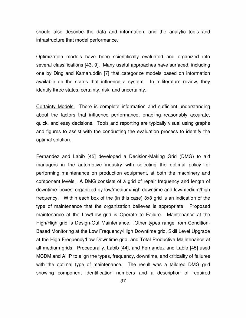
37
should also describe the data and information, and the analytic tools and
infrastructure that model performance.
Optimization models have been scientifically evaluated and organized into
several classifications [43, 9]. Many useful approaches have surfaced, including
one by Ding and Kamaruddin [7] that categorize models based on information
available on the states that influence a system. In a literature review, they
identify three states, certainty, risk, and uncertainty.
Certainty Models. There is complete information and sufficient understanding
about the factors that influence performance, enabling reasonably accurate,
quick, and easy decisions. Tools and reporting are typically visual using graphs
and figures to assist with the conducting the evaluation process to identify the
optimal solution.
Fernandez and Labib [45] developed a Decision-Making Grid (DMG) to aid
managers in the automotive industry with selecting the optimal policy for
performing maintenance on production equipment, at both the machinery and
component levels. A DMG consists of a grid of repair frequency and length of
downtime ‘boxes’ organized by low/medium/high downtime and low/medium/high
frequency. Within each box of the (in this case) 3x3 grid is an indication of the
type of maintenance that the organization believes is appropriate. Proposed
maintenance at the Low/Low grid is Operate to Failure. Maintenance at the
High/High grid is Design-Out Maintenance. Other types range from Condition-
Based Monitoring at the Low Frequency/High Downtime grid, Skill Level Upgrade
at the High Frequency/Low Downtime grid, and Total Productive Maintenance at
all medium grids. Procedurally, Labib [44], and Fernandez and Labib [45] used
MCDM and AHP to align the types, frequency, downtime, and criticality of failures
with the optimal type of maintenance. The result was a tailored DMG grid
showing component identification numbers and a description of required

38
maintenance. Management receives and reviews this grid and plans
maintenance accordingly. Labib [44] and also Khalil et al. [46] apply the same
process under the name of a Modified DMG. Here, failure cost was used as a
decision criterion instead of failure duration. Ding and Kamaruddin [7] cite
several studies where Fuzzy Logic (FL) was incorporated into DMG to improve
the effectiveness of maintenance for aerospace, food, and other manufacturing
industries. Gupta et al. [47], however, employ a different graphical approach
using control charts to identify appropriate maintenance practices for a conveyor
used in a coalmine.
Risk Models. They involve assumptions about complex systems using only
vague information due to low quantity or quality data. The condition and
performance states themselves are known, and can be modeled and optimized
stochastically through probability distributions and other methods. Given the
current condition, risk models can be used to predict future conditions determine
optimal maintenance. Ding and Kamaruddin [7] identify three types of risk
models, mathematical, simulation, and artificial intelligence models.
Mathematical models are the most frequently used [7]. The Cox Proportional
Hazard Model (PhM) can be used to model the influence that different covariates
have on degradation or the age of the system, compared to a baseline age of
that system under what are considered normal factors and conditions [48].
Martorell et al. applied PhM to model life distributions building nuclear power
plant working conditions, surveillance, and maintenance effectiveness into the
model [49].
Another common application is the Markov method. It too is a stochastic process
used to describe how a random variable transitions between different states of
condition or operation. Models can be as simple as having two states,
functioning or not functioning. They can be more complicated with multiple

39
states, each with specific distributions transitioning between states. Ding and
Kamaruddin [7] provide a literature review of studies and uses, including nuclear
power, locomotive diesel engines, coal transportation systems, air-blast circuit
breaker, etc. They also pause to mention modeling using probability density
functions, non-linear programming, classic logic with probability theory, mixed-
integer linear programming, Modified Powell method, and non-homogeneous
Poisson process, with particular attention to Bayesian pre-posterior decision
theory [7]. Bayesian updating is particularly attractive because it provides a
constructive and controlled path for combining new information with old, while
preventing the old data from dominating the new. The exact procedures for PhM,
Markov, and Bayesian updating will be detailed in the next chapter.
Simulation-based Modeling. It has become a popular method for exploring the
range of possible outcomes and densities (average and standard deviations) that
can be used to make well informed decisions [7]. Monte Carlo simulation uses
random sampling to combine different conditions and environments to derive
‘what-if’ outcomes not possible using other mathematical methods. It is
particularly useful for optimization where the interaction between different factors
is critical, but otherwise unknown. Simulation calls the concept of multi-
dimensional mathematical functions, indicating the need for and use of multi-
variable, multi-component, time-based data to develop the optimal solution to the
maintenance policy selection problem. Ding and Kamaruddin [7] provide a
literature review of studies and uses of Monte Carlo simulation, gas compression,
transmission system, electrical network, chemical plant, gear pump, motor
engine company, etc. They also pause to discuss particular applications,
including SIMSCRIPT simulation, discrete-event simulation, SIMAN simulation,
SIMUL8, data envelopment analysis with TOAD, and fuzzy discrete event
simulation [7].

40
Artificial Intelligence-based Models. They are “…concerned with computational
understanding of what is commonly called intelligent behavior and with the
creation of artifacts [models or algorithms] that exhibit such behavior… [7]”.
Genetic algorithms can be used to optimize maintenance policies, using
unsupervised methods (those that do not incorporate training data sets) on
binary data, and are slower to evolve compared to other methods, such as neural
networks. Ding and Kamaruddin [7] provide a literature review of studies and
uses of genetic algorithms, including those on series production line, emergency
diesel generator, concrete bridge decks, bridge superstructure, power
transmission, and motor-driven pump. They expand explaining Monte Carlo
simulation with genetic algorithms were applied to a model chemical processing
plant, high-pressure injection systems, and raw mill in the cement industry [7].
Uncertainty Models. They involve judgements about future conditions where
corresponding probabilities are unknown. In this case, information is obtained
from expert witnesses and derived subjective probabilities. Models include
heuristic, hazard-based, and multi-criteria models.
Heuristic Models. They apply ‘rule-of-thumb’ methods to logically derive the
optimal solution from experience and expert opinion. They are useful when there
is little information available or it is impractical to obtain in detail. In a series of
studies and applications, Waeyenbergh and Pintelon [50, 51, 52].use a decision
tree comprised of technical and economic objectives and factors to select the
optimal maintenance policy. Their process required asking experts and
members of respective organizations a series of questions that compare the
applicability and effectiveness of different aspects of maintenance policies.
Based on those answers, different individual ratings (weights) are assigned,
where the overall rating was used to select the optimal maintenance policy. They
go on to prescribe implementation and steps for follow through using a series of
Plan-Do-Act-Check actions. Ding and Kamaruddin provide a literature review of

41
studies and uses of heuristic decision tree models to select the best maintenance
policy for equipment in a thermal power plant, a drilling system, and the cigar
industry [7].
Hazard-based Models. They were developed to counter the trend toward
developing policies based on effects, rather than root-causes [7]. Hazard models
are dominated by FMECA and FTA activities due to their visibility and easiness
[53]. FMECA is used to classify every failure mode according to criticality and
number or probability. FTA is deductive, evaluating failures from top to bottom,
and causes for them. Li and Gao combine FMECA and FTA in models as part of
Root Cause Analysis (RCA) on a petrochemical plant [54]. FMECA and FTA
have weaknesses. They consider probability of failure, probability of non-
detection, and severity, ignoring other important aspects such as economic and
logistics considerations [53]. Expert staff and managers find it difficult to
effectively quantify these other factors, often inconsistently assigning different
weights of importance to criteria.
Ding and Kamaruddin [7] explain that in general, hazard-based models are
subjective, so Braglia et al. [53] developed a FL model to address the
“…imprecision, randomness, and ambiguity” of contemporary FMECA [53]. The
main problem with FL models is with implementation when defining rules and
membership functions; they can become unmanageable. Further research is
recommended for FL, although promising results have been found so far. Ding
and Kamaruddin [7] provide a literature review of studies and uses of hazard-
based models used to select the best maintenance policy for equipment in oil
refinery industry, power plant, water treatment plant, gasification plant,
petrochemical industry, flour process plant, paper mill, and a paper
manufacturing plant [7].

42
Multi-criteria-based Models. They involve MCDM techniques, the most widely
adopted approaches in maintenance policy optimization. The chief advantage of
MCDM is it provides a way to integrate multiple, usually conflicting objectives and
requirements into the decision process. MCDM helps to assign adequate weight
to more broad and important aspects of maintenance like safety to personnel, the
system, and environment; added value, like spare parts inventory, production
loss, fault identification; logistics support, and budget and funding issues. It is
easy to understand that not all of these other important factors are involved with
alternative methods that focus, principally, on cost, availability, reliability and
failure modes analysis. There are three major steps for implementing MCDM.
First, the organization is required to determine relevant criteria (goals, objectives,
and requirements) and alternatives (if not this type of maintenance, then that, or
the next type). Second, the organization is required to establish a weighting
system for both the criteria and alternatives. Finally, the optimal maintenance
policy is identified after calculating the relative ranks among alternatives. There
are three main types of models, Weighted Sum Model (WSM); AHP, and Fuzzy
Analytic Hierarchy Process. Other methods and tools include Elimination and
Choice Translating Reality (ELECTRE), and the Technique for Order Preference
by Similarity to Ideal Solution (TOPSIS) [7].
The simplest and probably still most widely used MCDM is the WSM. Where
maintenance planning is concerned, the process begins by assigning
maintenance policies numerically to different levels of preference. Assuming all
criteria have common units, importance (weights) are assigned to each criteria,
which are then summed to calculate the level of preference, and subsequently
identify the appropriate maintenance strategy [7, 55]. This method has some
weaknesses. The process assigns ‘actual weights’ that reflect the ‘subjective
opinions’ of the organization. They are not always accepted because subjective
weights are sometimes insensitive to global or local environments.

43
An alternative approach that makes use of the same preference, importance, and
criteria is AHP. It was applied to failure analysis by Braglia and Bevilacqua
(2000) [53]. With AHP, the process for establishing weights is more widely
accepted. It typically entails a tree structure, using top-down decomposition and
pair-wise comparisons to assigning weights to criteria [55]. As with WSM, AHP
can be used to identify the best-suited maintenance plan. However, simulation is
recommended to develop the optimal maintenance plan. So to this end, the
critical criteria should be identified. The critical-criteria is often thought of as the
one with the highest weight. This is misleading. The critical criteria, however, is
the criteria for which the smallest change has the greatest impact on the type of
decision that is being made. For the purpose of this paper, the decision is
selection of the optimal maintenance policy. In addition to conducting AHP and
simulation, the organization should identify the critical criteria and identify the
range needed to transition from one type of maintenance policy to another of
greater perceived benefit. Ding and Kamaruddin [7] provide a literature review of
studies and uses of AHP models used to select the best maintenance policy for
equipment in oil refineries, oil pipelines, virtual learning facilities, the wind turbine
industry, the textile industry, news printing industry, automotive manufacturing, a
chemical plant, and a power plant.
Fuzzy Logic AHP is discussed extensively by Ding and Kamaruddin [7], but will
not be detailed by this paper. FL AHP is listed here due to its relevancy and
promise for the future. Ding and Kamaruddin cited studies and uses of FL AHP
models used to select the best maintenance policy for equipment in oil refineries,
the benzene extraction industry, the textile industry, air craft industry, the
semiconductor industry, and the copper mining industry.

44
2.5.3 Frequency of Publication In completing the previous subsection, it is concerning to find so many methods
available to use for selecting a maintenance policy. Maintenance communities
and industries have yet to identify the definitive method. To better understand
the spread in efforts to reach unification and focus on where the global
community stands now, the following sources and discussion provide context to
concepts discussed earlier.
In a literature review by Garg and Deshmukh, 157 papers were collected and
analyzed to organize methods and techniques into six broad classifications of
topics and publish dates [56]. They are summarized in Tables 11 through 13 of
Appendix A for review and discussion below.
The Garg and Deshmukh study, summarized in Tables 11 and 12, indicates that
from 1995 through 2006, there has been a steady increase in the volume of
research into methods for optimizing maintenance, with little published before
this time period. Further, there has been considerably more research devoted to
maintenance techniques compared to methods for optimization, performance
measurement, and maintenance policies; with relatively little focus on scheduling
and information systems. According to this study, activity peaks between 2001
and 2002.
Garg and Deshmukh offer the following insight. Maintenance plans become
“…immediately out of place as soon as an emergency job…” or some other
disruption is inserted into the system. The impact that disruption has on
maintenance scheduling continues to be an underserved area in research and
practice. It should be carefully considered when identifying optimal maintenance
policies [56].

45
In a separate literature review of maintenance optimization by Sharma, Yadava,
and Deshmukh, they collected and evaluated a series of published literature
reviews, categorizing sources by maintenance optimization models and case
studies [57]. In their evaluation, they distinguish and focus exclusively on ‘real’
publications; those published only after review by academia and researchers who
include the model, data, and application. Their findings discussed below are on
the ‘real’ publications by Sharma et al. [57]. The purpose for their study and
discussion here is to continue to uncover the broad scope of topics involved with
maintenance optimization, and better understand the maturity of optimization
principles and practices.
Table 14 indicates an increasing number of publications on failure rates, cost,
and optimization. Tables 15 and 16 demonstrate from 1997 to 2007 an
increasing number of publications in all categories; optimization, mathematical
modeling, and preventive maintenance.
The results of Sharma et al. [57], shown in Figure 30 in Appendix B, are
consistent with those from Garg & Deshmukh. Where maintenance optimization
is concerned, there appears to be little ‘real’ literature published before 1997.
The number of published literature peaks between 2000 and 2002, with the bulk
center found in the early to mid 2000s. Both studies show a decline towards the
late 2000s.
Sharma et al. [57] discuss the following important considerations and
conclusions. With companies adopting policies that use maintenance to improve
profit, aligning maintenance practices with corporate objectives is more important
now than ever through value added activities, such as data collection, analysis,
and automated feedback mechanisms. They explain that optimal maintenance
for multi-component systems should simultaneously consider cost, reliability, the
applied maintenance policy, and other factors that enable or constrain the

46
business model. Many of the methods require a new Corporate Philosophy and
long-term commitment. Mathematical models are ineffective without a system
that collects and analyzes data on operations, maintenance, degradation, cost,
and modifications. They conclude the gap between theory and practice is still
very wide. So more needs to be done to implement and demonstrate the
effectiveness of these methods. Information Technology (IT) as a tool and
enabler of optimized maintenance continues to be an underserved area. Its
appearance in literature and general use is expected to continue to decrease in
cost and increase in availability for the everyday user. The models use to
optimize maintenance have had little impact on making decisions, so
demonstrated effectiveness has been limited. To improve, Garg and Deshmukh
recommend developing a common definition of the problem to solve, training on
economics and its place in maintenance, as well as training on the principles of
optimization and use of IT-enabled systems. In closing, optimization models are
useful if the staff is capable of incorporating information on the conditions,
degradation, and the maintenance strategy back into the general maintenance
system.
2.5.4 Benefits The benefits of different maintenance strategies, policies, tactics, and methods,
like all things, depend on a large number of factors. That is why there is not a
best practice for selecting a maintenance policy, and no standard cost reduction
or profit increase to achieve. Benefits are identified by how an organization
measures improvement. Without improvement, the organization will not accept
the added effort and expense as beneficial. To that end, the benefit of a
maintenance strategy is a function of how close (in some form of measurement)
the current approach is to alternative approaches, and the organization’s
capability and commitment to implementing and sustaining beneficial
alternatives.

47
Swanson [58] measured the perceived benefits of different maintenance
strategies in his study. 708 surveys were sent to 354 manufacturing plants,
where 287 respondents returned completed surveys. Various factors were
considered for each respondent such as age, occupation, size of plant, and plant
maintenance budget. Respondents were asked to provide ordinal values
measuring the importance of different aspects of the maintenance program, and
its affects on quality, equipment availability, and production costs. Respondents
did so for three categories of maintenance, aggressive, proactive, and reactive.
Swanson used principal component and multiple regression analysis to extract
features from the responses. Swanson found that aggressive and proactive
maintenance strategies are associated with improved performance, concluding
that transitioning to these will provide a benefit. Likewise, reactive strategies are
associated with lower performance. Further, certain processes and practices are
required to ensure a transition will provide a benefit. For a proactive strategy,
equipment monitoring and analysis is required. For an aggressive strategy,
proactive elements are required as well as feedback and design changes [58].
Koochaki et al. [59] examine the influence that CbM has on workforce planning
and maintenance scheduling. CbM, in a theoretical application, is performed
just days or weeks before a failure to maximize up-time and minimize life cycle
costs. This approach implies just-in-time repairs. Koochaki et al. [59] explain the
problem with CbM is with scheduling downtime and obtaining materials and
services. In practice, while organizations may claim that they do CbM, what they
actually do is opportunistic or block maintenance, where the system or whole
areas within a plant are taken out of service to repair failed components and
perform early or overdue maintenance on others.
Koochaki et al. [59] explain that most research, and theoretical and fielded
methods measure the benefits of maintenance on a single component, whereas
there is little research and feedback from the field on multiple components. In

48
their study they evaluate the efficiency of predeterminative (age or time-based
replacement; TdM) and CbM by the operational availability of the plant. They do
so for two configurations, three components in series, and separately three
components in parallel, for both ideal maintenance, where maintenance prevents
all failures, and non-ideal maintenance which prevents only some failures. An
important feature is that TdM allows scheduled downtimes and subsequently
regular workforce and material sequencing. CbM does not, so blocking and
opportunistic downtimes are built in to the analysis. Another important feature is
systems repaired in parallel can be repaired in a shorter period of time, but with a
larger workforce. Conversely, systems repaired in series take longer, but enable
a smaller workforce. And finally, systems designed for high maintainability are
best maintained by organizational level mechanics with general knowledge and
capability; they can perform maintenance at any time, reducing downtime for
sequencing and other logistics. They find that efficiency is slightly better under
CbM compared to TdM for the parallel configuration because there is a longer
average time between maintenance events. In the serial configuration, however,
CbM has a slightly lower efficiency than TdM because more systems can be
grouped together, reducing the need for inefficiencies built into the system for
blocking under the pretense of CbM. Where cost, not efficiency, is concerned,
CbM out-performs TdM. The authors note, though, that TdM results in a much
smoother maintenance plan, especially when ideal maintenance is performed
[59].
In a separate study, Koochaki et al. [60] examine the effectiveness of CbM in a
plant-wide, multi-component environment. They begin by explaining that there is
no known research and return data on CbM simultaneously applied to multiple
systems. They go on to express that this is justification for stating “…CbM
programs are not always in line with the holistic maintenance goals of the
organization [11].” Expanding on their earlier work, they explain that
opportunistic maintenance is a policy for systems-of-systems, creating efficiency

49
for maintenance crews by combining maintenance on several components into
the same timeframe, reducing costs and increasing availability through
economies of scale. The concept of opportunistic maintenance itself is based on
economic dependency among the components [11].
In a bold statement, Koochaki et al. [60] said “…theoretical advantages of CbM
for plant components are not necessarily transferable to the plant level.” CbM,
however, can be used to provide the right information to schedule maintenance
for an opportunistic maintenance timeframe. This is a period of time when
degradation has started, is observable, and maintenance makes sense, but
before functional failure and shutdown of operations. To aid in identifying this
timeframe, Zheng and Fard [61] propose establishing a hazard rate tolerance.
When a component within the system exceeds its hazard rate, all other
components within specified thresholds are replaced at the same opportunistic
time period [61]. This approach neglects the tranditional MTTF, and assumes all
components use the same maintenance policy.
To better understand the effectiveness of CbM, Koochaki et al [60] performed an
experiment where they used sensitivity analysis to investigate a different number
of components under CbM and TdM with the following factors: different lengths
of opportunistic maintenance; economic dependency among components; and
the probability of failure within a PM interval. They compared benefits in terms of
Line Productivity (LP) (% increase of production) and total maintenance costs,
finding the following:
• Without opportunistic maintenance, LP increases when more components
use CbM because there are fewer maintenance events, and longer uptimes.
• With opportunistic maintenance, maintenance of components is
synchronized, increasing the number of group events, decreasing, however,
the total number of events for the system.

50
• If the maintenance opportunity zone is increased, then more opportunistic
maintenance is performed, improving LP.
• Increasing the number of components that use CbM decreases the
effectiveness of opportunistic maintenance because TdM components under
opportunistic maintenance have more total maintenance events.
• Given the factors and constraints of the study, LP efficiency for multi-
component systems is improved through an opportunistic maintenance
strategy that uses TdM, rather than increasing the number of components
under CbM.
• Opportunistic maintenance can decrease total maintenance costs, whereas
the effect is largest when all components are under TdM and smallest effect
when all components are under CbM.
• Opportunistic maintenance results in shorter PM intervals, more group
maintenance events, and fewer total number of maintenance events, thus
decreasing annual maintenance costs and decreasing corrective
maintenance events under the TdM policy.
• The higher the economic dependency between opportunistic maintenance
components, the lower the maintenance cost potential.
They conclude as follows [60]: There is no single optimal maintenance policy for
a multi-component system for cost and line production. In an experimental
setting, implementing CbM for all components under an opportunistic strategy
would [theoretically] minimize cost, but not LP. Setting all components under
TdM and opportunistic maintenance would maximize LP, but not cost. So if cost
is more important, then strict CbM or CbM under opportunistic maintenance may
be optimal. If LP and regular schedules are more important, then TdM may be
optimal. The intent is to use this information to better manage the trade space
between cost and efficiency (availability) [11].

51
2.6 (Levels 6 & 7) Prognostics and Health Management
This section is organized similar to how a PHM system should be designed, from
the top-down and outside-in, discussing first the purposes, uses, and features;
and later specific analytic methods. Earlier sections of Chapter 2 were dedicated
to organizational structures and behaviors, requirements, types of maintenance,
and processes that enable optimal maintenance. All of those things must exist,
and be effective and suitably functioning to enable PHM [8]. In the following,
specific principles and processes of PHM that optimize performance and
maintenance of a specific component, operating in a specific environment, under
specific conditions will be examined.
A well conceived PHM system is instituted at the enterprise level,
comprehensively supporting the maintenance and health of a number of systems
through common infrastructure. It should be designed and integrated during the
development phase of the equipment life cycle to serve all phases of life through
the highest levels of organizational performance and improvement, a proactive
maintenance policy and TPM approach. The PHM system should provide
information to operators enabling on-condition changes in operational states that
ensure safe operations and optimal service lives, as well as provide information
that support CbM and opportunistic maintenance workforce scheduling, material
ordering, and other logistic issues that reduce downtime and aid in controlling
production schedule. Illustrated by red dashed lines in Figure 1, it should also
provide information back to designers responsible for developing new products,
and also to operators and maintenance managers who are responsible for
developing modernization changes that increase the maintainability and reliability
of in-service equipment. A PHM system is an enabler that unlocks the cost
cutting, operational availability and profit increasing potential that resides within
equipment SoS.

52
A PHM system senses, collects, stores, and analyzes data, and reports
information that can be used to detect abnormal performance and diagnose
faults, detect and quantify degradation, and can be used by operators to make
maintenance decisions based on projection of the remaining useful life of the
equipment. Advanced versions integrate with decision, operating, and
maintenance management systems to automatically change operational setting
and initiate maintenance, thereby increasing safety, and reducing downtime, the
number of personnel involved, costs, and inconsistent human decisions.
As with the concept of affordability discussed earlier, PHM can be used to
manage the trade space between material performance, safety, maintenance
cost, and logistics support. Figure 8 below, adopted from Peng et al., illustrates
an idealized relationship between RUL, reliability, and maintenance cost [62]. It
indicates that there is a local minimum in the cost curve, indicating the time when
it is best to perform maintenance for the lowest cost. Reading along the
horizontal axis of decreasing remaining useful life, the time when maintenance
should be performed for the lowest cost appears to be when the reliability curve
has a rapidly decreasing change, typically when the system is wearing out.
Figure 8. Relationship Between RUL, Reliability, and Maintenance Cost [62]
RUL
Source: Peng et al., "Current status of machine prognostics in condition-based maintenance: a review", 2010

53
The remaining sections of this paper will focus only on the data and analytical
features that are used to identify optimization. Figure 9 illustrates major features
and relationships of a PHM system that manage data and analytics. In an ideal
situation, a population of historical data is evaluated to identify features that are
known or are thought to be important to making a decision about the health and
maintenance of a system or component. Relevant features are then extracted
and used in a supervised environment to train a set of data from which certain
test and validation functions are performed in the process of conducting
diagnostics and prognostics on the equipment [62].
PHM works best with continuous real time data, which can be combined with
historical data. Monitoring and anomaly detection correct certain errors within
the system, estimating the true value of feature variables [63]. Estimates are
compared to the true values, creating residuals, which are then monitored for
abnormal deviations, indicating anomalies or degraded performance. Noise and
noise reduction is also considered. Diagnostics are used to isolate areas or
specific components where faults have occurred, and estimate the root cause for
a change in performance. Prognostics then, rely on physics based or empirical
models to understand the relationship between changes in performance and the
RUL. Diagnostics are useful for improving new in-service equipment.
Prognostics useful for planning maintenance and extending the life in-service
equipment.
Tiddens et al. [8] present six postulates discussing factors that prevent PHM from
working properly.
Postulate 1 - Often, data are not useful for advanced analysis. More mature
companies have a lot of data with sufficient storage and retrieval. Smaller
companies have trouble accessing useful data because it is often incomplete and
stored in multiple locations. Operators often refuse to enter the correct data

54
Feature Selection
Sele
cte
d D
ata
Sele
cte
d D
ata
Sele
cte
d D
ata
Sele
cte
d D
ata
Data Training
Historical Data
Monitoring-Anomaly and Detection,
Diagnostics & Prognostics
Reliability & RUL Reporting
Maintenance Schedule
Real Time Data
Verification
Cost Function
Feedback To New
Development & Modernize InService
Level 6
Level 8
Level 7
Figure 9. Notional PHM System

55
because the maintenance system is complicated and new to them. Even when
data are uploaded and stored real-time, they are often difficult to access because
file sizes are too large to be transferred.
Postulate 2 - Selection of parameters to monitor is not well motivated. When a
new system is fielded, often the exact parameters for evaluation are not
immediately known. So organizations collect a lot of data on many parameters,
sometimes missing those most important to system performance or maintenance
managers.
Postulate 3 - Higher levels of analysis result in higher value analyses. This is the
expectation, but it is not always true. Operators and mechanics are sometimes
more useful than continuous monitoring sensors. They can see, smell, hear, and
feel many different conditions; sensors do that for very specific conditions.
Postulate 4 - Predictive performance of prognostic systems improve over time;
they are evolving systems. When the equipment is new, we do not know how it
will perform. After a period of time, the experience gained and data collected
helps to better interpret signals that indicate changes in performance.
Postulate 5 - Selection of advanced maintenance analysis is not well motivated.
More mature companies are better positioned to perform advanced analyses.
Less mature, though, use straightforward methods - FMECA and common sense.
Another respondent said “Sometimes we try a particular method. When this
doesn’t work, we will try another method…we find a nice software package which
enables its use… [8].”
Postulate 6 - The quality level of current analyses is not sufficient to improve
maintenance decisions. Of the companies that were queried, current data
analyses were known to be imprecise, so applying more advanced PHM
56
methods was not believed to provide markedly better results from which
maintenance decision can be made. One respondent said “Our FMECAs are
used for long term prediction. Resulting maintenance intervals are rather
conservative, therefore maintenance is often conducted too early.”
2.6.1 Data Management There are many topics on data management that are critically important for
accurate PHM. They will be incorporated into the analysis used in later sections,
and only briefly mentioned below because they distract focus from ‘bigger
picture’ strategic maintenance policy selection and use of PHM.
2.6.1.1 Multidimensional Data & Data Cubes
The accuracy of anomaly detection and diagnostic and prognostic algorithms
depends heavily on the number of assessment readings, assessment reading
frequency, and the number of different features (variables) used to describe
component condition, use, behavior, and operating environment. Analysis using
binary data, like ‘failed’ or ‘not failed yet’, yield marginally informative results [8].
Anomaly detection and diagnostics must use a wide variety of complete data to
be effective. Prognostic projections of future conditions are improved greatly by
the number of relevant features and frequency of readings.
For this project, the term ‘features’ is synonymous to ‘dimensions’; they describe
different ways the performance of a component can be evaluated. If an analyst
is evaluating different failure modes to identify the root cause for a failure, that
means they are exercising a multidimensional root cause analysis.
Multidimensional analyses often incorporate different numbers and combinations
of independent variable (features) to measure the influence or effect that each
has on the dependent response variable.

57
The multidimensional structure of data is often viewed as a cube with three-
dimensional coordinates for each data element [64] [65]. Each dimension within
a three dimensional cube can represent, for example, x-dimension as the
features or failure modes under investigation, y-dimension as the values
recorded during successive readings or inspections on individual components,
and the z-dimension as the number of components on which x-features, and y-
number recordings are made. A fourth dimension of time is implied to occur at
regular frequency along the y-axis, illustrated in Figure 10. In the figure it shows
the common x-dimension as ‘s’ for sensors, y-dimension is ‘j’ for observations, z-
dimension is ‘k’ for components, and the fourth dimension of time is ‘i’ for time or
frequency.
When the enterprise level system is designed, it is important to understand how
the database should be structured to support the analysis that is used to make
maintenance decisions later on in the process. This influences the way data are
collected and transmitted to and from the field, ultimately affecting the fidelity and
accuracy of conclusions and predictions.
2.6.1.2 Types of Variables
Tamhane and Dunlop explain that features or characteristics of interest are
called variables, and that data are their measured values [66]. Tamhane and
Dunlop, along with Hellerstein [67], describe different categories of variables.
Qualitative variables are typically identified as nominal or ordinal. Nominal
variables describe labels; e.g. red, yellow, green. Ordinal variables represent
rank or order; e.g. 1 is low, 2 is medium, 3 is high.
Numerical variables are typically identified as continuous or discrete. Continuous
variables are from a set of numbers or from a common unit of measurement; e.g.
time. Discrete variables are from a defined set; e.g. number of pieces of

58
Prognostics
Anomaly Detection
& Diagnostics
Figure 10. Data Cube Structure

59
equipment [66, 67]. These concepts play an important role for understanding
limits in accuracy from different types of analysis. An inspection program that
collects qualitative data, or only discrete (ordinal) values, provides less
informative information compared to one that collects continuous data which
provide the most information. An optimally performing system strives to collect
the most informative data.
Fienburg [67] assigned ordinal rank – weight – to categorical variables when he
evaluated the randomness of the US 1970 draft lottery. In 1970, public outcry
over the conduct of the war draft heightened inspection into its conduct. The
process consisted of inserting January dates into 31 capsules, February dates
into 29 capsules, and so on. They were poured into a box, separated, and
ordered by month. The box was shaken several times to randomize the capsules
before they were poured out into an open container, where several thousand
drawings were made each day for 31 days. The public claimed the process was
unfair because it was not random. When Fienburg studied the issue, he first
plotted the number of capsules selected during each day of the drawing by birth
month-category. While the plot showed a reasonable spread in the data, some
regions were sparely populated, and others had slight clumps of data. To
determine if selections made for some birth months outweighed selections made
for other month, he took the average number drawn for each month. The result
found significant bias for selecting capsules for birth months early in the calendar
year compared to those selected for months later in the year [68]. After
interviews, Fienburg concluded several causes for bias – initial separation by
month; inadequate shaking; pouring from the end of the box with later calendar-
year months first placed at the bottom and early months at the top; and selecting
capsules located at the top. This method of assigning ordinal rank was applied
to variables used in these analyses.

60
2.6.1.3 Collecting, Cleaning, and Storage of Data
Before, during, and after data enter a database, errors often creep into the
system through data entry, measurement, distillation (when raw data are
preprocessed and summarized), and integration (data combined from different
sources) errors [67]. To reduce the number of errors, a number of steps should
be taken. Through ‘interface design’, an organization can incorporate integrity
constraints in the graphical user interface and storage system by controlling,
often limiting, the types of data that can be entered; pull-down menus are helpful.
‘Organizational management’ approaches call on the Total Data Quality
Management concept to use technological solutions that streamline data
collection, archiving, and analysis, incentivizing all parties to align with single
processes. ‘Automated data quality and cleaning’ uses technology to identify
and correct errors. ‘Exploratory data analysis and cleaning’ is the most common,
requiring a validator to review, identify, initiate, and follow through with correcting
errors. Common errors include missing and stuck data, and multiple entries of
the same value (for which multiple entries of the same value is considered
unusual).
Cleaning quantitative data. Quantitative data consist of numbers with
dimensions that can be measured in terms of distance (spread or variance) from
each other, with consistency among units of measure. Statistical methods for
outlier detection are the most commonly used approach to managing quantitative
errors. It is worth mentioning that outliers are often not included in analyses.
They should not be discarded, but kept and evaluated because they may provide
the best information for evaluating inefficiencies in a system and causes for
failure in equipment. An organization’s view on the definition of outliers is
subjective, often reflecting the weight of importance they place on the item under
investigation [67].

61
Cleaning categorical data. Categorical data typically have no natural distance
between values, so evaluating errors by outliers is not possible. For these, errors
often occur when a subcategory value is incorrectly mapped to a ‘master
category’. Another type of error is typos or misspellings. Limiting data entry to
discrete subcategories and pull down menus is helpful for managing these errors.
Cleaning postal address or free text data. Postal address and free text data are
very difficult to record, manage, analyze, and report. They should be limited and
discouraged within a database.
Cleaning Identifier data. Identifier data typically are used as keys that assign
membership to a particular group. Challenges include detecting and correcting
reuse, or loss of association when multiple databases use the same data, but in
a different context; e.g. used as an identifier in one database, but subservient
data element to another identifier in a related database.
2.6.1.4 Data Exploration
This topic is very important when designing data collection programs and before
analyzing data. Standard statistics textbooks provide sufficient instruction on
evaluating the means and variance of populations and samples, and with
identifying and evaluating outlying data.
2.6.1.5 Training, Test, and Validation Groups of Data
Tamhane and Dunlop recommend the following approach when building
regression models; it can be applied to other model building exercises as well
[66] [69]:

62
1. Determine the type of model needed for analysis. The type of model dictates
the type of variable data.
2. Collect the data. Before beginning, determine independent predictors and
dependent response variables so the structure for analysis is well understood.
3. Explore the data. Examine it for errors, outliers, missing values, and biases.
At this point, erroneous, unwanted, or unneeded data should be corrected or
removed.
4. Divide the data into training and test sets; Afendras and Markatou [69]
discuss a third set for validation. All of the data should be divided in a
constructive way (even/odd, venetian blinds, random, or visual inspection)
that populates these three sets. The training set should be used to build
models and fit parameters. They should include data that covers the full
range of values (for quantitative data, the largest and least) observed in the
field. Test sets are used to optimize the models, including cross-validation to
avoid overfitting. Over-fitting is when the model fits historical data very
closely, but is not likely to fit other data in the future as well. A validation data
set is used to characterize performance, indicating the best performing model
of those used for analyses.
5. Fit several candidate models. This is the training set.
6. Select and evaluate a few good models. This is a combination of training and
test sets discussed above.
7. Select the final model. This is from the validation set.
Combining data with different units while retaining relationship. This is
accomplished by calculating the mean-center-unit-variance for covariates [70]. If,
for example, the performance of a pump is evaluated by sensors that collect data
on vibration, amperage, temperature, and revolutions per minute, it is difficult to
calculate the response or cause for failure if covariates remain in their current
form (units). After transforming them to a common form of variance about their

63
respective means, analysis can then evaluate spread in the data, identifying
relationships and abnormal behaviors.
2.6.1.6 Treatment of Censored Data Allison explains that survival analysis is a class of statistics that studies the
occurrence and timing of events [71]. Often, this involves using condition data
analysis or life data analysis to fit certain life functions to data; calculating the
parameters of functions that most closely reflect performance in the field. Where
life data analysis is concerned, it can be used to extract features from those
parameters that describe conditions or environments that contribute most to the
occurrence of events. For PHM, continuously recorded data provides the best
information. Often though, especially when reviewing data collected in the past,
it is not continuous. In these cases different techniques are needed to deal with
the time-value of incomplete or ‘censored’ data.
Where censoring is concerned, complete data is when the exact time of event is
known. For right censored data, also known as suspended data, the test is
stopped (analysis is performed) before failures occur. For left censored data,
failure times occur before the test is conducted. For interval censored data,
failures occur between two known times. Multiply censored studies involve
complete, right, left, and interval censored data, or any combination thereof.
Type I censoring involves conducting tests for a fixed length of time. Type II
censoring involves conducting tests until a predetermined number of failures
occur [2, 71, 72].
Singh and Totawattage [72] explore more commonly used methods for managing
censored data, ultimately concluding that parametric models provide better
results compared to non-parametric models. Their advantage is in applying
specific conditions and environments to more accurately model performance for

64
the specific component or system. Their disadvantage is often there is not
enough data that can be used to develop models and optimize parameters [72].
2.6.1.6.1 Parametric Methods
Singh and Totawattage suggest using the Accelerated Failure Time (AFT) to fit
life distributions (functions) to interval censored data [72]. Procedurally, AFT is
used to calculate failure times, from which life distributions are fit according to
their respective parameters.
AFT models are parametric models similar to the PhM. PhM assumes the
covariate has a multiplicative effect on a basic hazard function, Equation 1. H�
represents the hazard rate for an individual with covariate z. H� represents the
basic hazard rate if the contribution from any and all covariates is zero. β
represents regression coefficients for different covariates (factors). If β is
negative, then the covariate z has the effect of speeding up the hazard rate.
H� = H�e�� Equation 1
AFT similarly assumes the covariate has multiplicative effect on a predicted time
event by some constant, Equation 2. T� represents the failure time. T�
represents the basic failure time. Other terms are the same as those in Equation
1.
T� = T�e�� Equation 2
Continuing, taking the natural log, and expressing log T� as μ + σW, the AFT
model is shown in Equation 3, where terms can be substituted and a linear
function derived as shown in Equations 4 and 5 in the SAS PROC LIFEREG
module. μ represents the intercept parameter. σ represents the scale
parameter, and W represents error [72].

65
log T� = log T� − βz Equation 3
log T� = μ − βz + σW Equation 4
log T� = μ + βz + σW Equation 5
In this final form, estimates of time of events for different conditions can be
estimated.
It is important to note that in their multi-application on breast cancer data, AIDS
data, and hemophilia Data, Singh and Totawattage [72], and others cited in the
study, found parametric methods resulted in reduced error compared to non-
parametric estimation methods.
2.6.1.6.2 Nonparametric Methods Nonparametric methods are typically characterized by steps of declining
magnitude in probability plots.
Kaplan-Meier Estimator (KM). KM is the nonparametric maximum likelihood
estimate of the survival function. It is one of the most common methods used
because it is simple to construct and well suited to incorporate censored data.
When a sample is large enough, or there is no censoring of the population, KM
approaches the actual survival function. The estimator is shown in Equation 6. ����� represents the survival as a function of time. n� represents the number of
survivors just before time t. d� represents the number of deaths at time t [72].
S��t� = ∏ !�"! !#!$# Equation 6

66
Turnbull Estimator. Peto was the first to recommend a nonparametric method for
estimating survival in 1973 [72]. In 1975, Turnbull derived the same estimator,
but used a different approach [73]. He published his iterative self-consistency
algorithm described in the following narrative and steps.
When survival times for candidate equipment are considered independent
random variables with survival function Equation 7, and failures are not directly
observed (occurring within an interval), then the likelihood of survival is explained
by Equation 8.
S�t� = Pr �T ≥ t� Equation 7
L = ∏ )S�L�� − S�R�+�, � Equation 8
Step 1 - Compute probability of event occurring at time tj.
p. = S/t.�01 − S/t.1, j = 1, … , m Equation 9
Step 2 - Estimate the number of events that occurred by time tj.
d. = ∑ 8!9:9∑ 8!;:;<;=> �?0 , j = 1, … , m Equation 10
Step 3 - Compute estimated number at risk at time tj.
n. = ∑ d@A@?. Equation 11
Step 4 - Compute and update the Product-Limit estimator (Equation 8) using the
pseudo code from steps 2 and 3 above until the updated survival value is close
to the old values of t.

67
Other nonparametric methods include logspline estimation of the survival curve,
and calculating the mid-point or extreme lower or upper observation times to
estimate failure times from censored data.
In their study, Singh and Totawattage [72] performed several experiments. One
experiment compared plots of two treatments of breast cancer patient data using
the mid-point method and KM, finding the results to be very similar. At most
times, the study found that the mid-point plot was either above or below (over-
under estimation) the KM interval plot. They go on to explain that over-under
estimation becomes more pronounced when estimates are taken at the lower or
upper bounds of the censoring interval, and even more pronounced with long
intervals [72].
They applied three different approaches to evaluate breast cancer, AIDS, and
hemophilia data. First, they used the parametric approach with assumed
baseline hazard rate to fit exponential, Weibull, gamma and generalized F
distributions. Second, they used what they call a flexible or semi-parametric
strategy by making ‘mild’ assumptions about the baseline hazard rate. And third,
they used a non-parametric strategy to estimate parameters, leaving the baseline
hazard rate unspecified. For the general effect of using chemotherapy on breast
cancer patients, they found that all analyses provided similar results. Where the
individual effects of stage and dose of treatment are concerned, they found non-
parametric methods did not perform as well as parametric methods. With the
AIDS data, which was heavily censored, they found non-parametric methods
lead to unstable estimation of time of events. They had similar findings for
analysis on the hemophelia data set, concluding that Weibull and log-normal
distributions provide the best results.
68
2.6.2 (Level 6) Health Monitoring
The term Health Monitoring refers also to performance monitoring of systems or
components.
Ramachandran et al. explain that the Condition Monitoring and Diagnostic
Engineering Management (COMADEM) was developed in 1987 to provide a
cross disciplinary approach to monitor, diagnose, prognose, control, and manage
complex systems throughout their life cycle [74]. In this context, the following
terms are used. The ‘condition’ of a system refers to how well its integrity and
intended reliable performance are ‘monitored’, scrutinized, and controlled under
specified operational and environmental conditions. ‘Diagnostics’ refers to the
critical analysis that determines the causes and effects of failure modes.
‘Prognostics’ refers to methods used to project the time when symptoms will
occur enabling prevention and control of failures. Finally, effective ‘engineering
management’ uses all of these and other resources to resolve problems that
prevent monitoring, diagnostic, and prognostic methods from working.
Condition monitoring is applied through continuous monitoring or periodic
monitoring. Both approaches rely on sufficient evaluation of failure modes and
historical data during system development to identify parameters needed for
monitoring and baseline data from which abnormal performance can be detected.
Continuous monitoring is necessary for critical machines and sometimes
necessary for essential machines to alarm operators or other mechanisms to
shut them down before damage occurs. Periodic monitoring, then, is performed
on essential machines and recommended for general purpose machines at fixed
intervals to forecast future conditions and maintenance planning. Figure 11
below, adapted from Ramachandran et al. [74] illustrates these uses.

69
Figure 11. Condition Monitoring Applications [74]
Moubray identifies six distinct patterns of failure, modeling system condition as a
function of time through the P-F interval [10]. ‘P’ is the time after a fault occurs
that could lead to functional failure, and when it becomes detectable. ‘F’ is the
time when functional failure occurs. The P-F interval, then, is the warning period,
during which assessments, maintenance planning and execution should occur.
Moubray [10] generalizes in his recommendation to perform assessments at
successively shorter intervals within the P-F interval. Figure 12 below illustrates
this method and its relationship between signal-alarms and the conditional
probability of failure which is often modeled using the bathtub curve.
Ramachandran et al. [74] present a slightly different model, illustrated in Figure
13, making use of an alarm threshold and upper limit. It describes a region of
stable performance until such time that an alarm signals the onset of failure.
After that, the failure zone continues until the upper limiting condition occurs and
the system is considered failed. Several useful calculations can be made from
Source: Ramachandran et al., "Recent Trends in Systems Performance Monitoring & Failure Diagnostics", 2010

70
this model. An estimation of the time (t) that has lapsed since the alarm point is
presented in Equation 12. The Remaining Time until a Functional Failure (RTFF)
is presented in Equation 13. Both of these equations are cited by
Ramachandran et al. [74].
Figure 12. Idealized P-F Interval
Ramachandran et al. [74] present a slightly different model, illustrated in Figure
13, making use of an alarm threshold and upper limit. It describes a region of
stable performance until such time that an alarm signals the onset of failure.
After that, the failure zone continues until the upper limiting condition occurs and
the system is considered failed. Several useful calculations can be made from
this model. An estimation of the time (t) that has lapsed since the alarm point is
presented in Equation 12. The Remaining Time until a Functional Failure (RTFF)
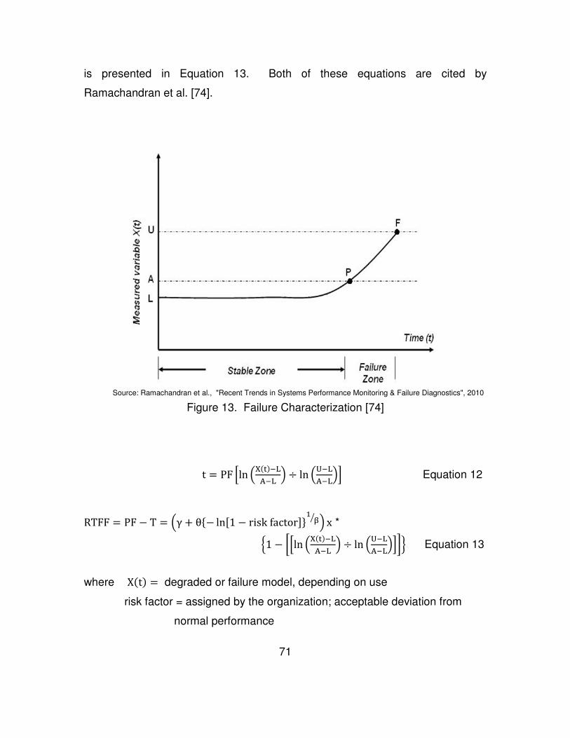
71
is presented in Equation 13. Both of these equations are cited by
Ramachandran et al. [74].
Figure 13. Failure Characterization [74]
t = PF Cln DE�#��FG�F H ÷ ln DJ�FG�FHK Equation 12
RTFF = PF − T = Dγ + θ)− lnN1 − risk factorU,0 V H x *
X1 − YCln DE�#��FG�F H ÷ ln DJ�FG�FHKZ[ Equation 13
where X�t� = degraded or failure model, depending on use
risk factor = assigned by the organization; acceptable deviation from
normal performance
Source: Ramachandran et al., "Recent Trends in Systems Performance Monitoring & Failure Diagnostics", 2010

72
There are several methods for detecting anomalous behaviors. There are first
principle models, such as those used to evaluate ball-bearing wear. And there
are empirical models which are helpful when characterizing performance in the
context of specific operational environments. Where statistical models are
concerned, evaluation of residuals is particularly helpful for characterizing
performance away from that normally observed [63, 70]. Other methods include
thresholding techniques and hypothesis testing, such as the Sequential
Probability Ratio Test [63, 75].
2.6.3 (Level 7) Diagnostic Methods
For these purposes, faults are understood to mean abnormal or unintended
behaviors or performance. Faults are diagnosed using isolation techniques that
focus the investigation on the performance of specific components or features for
root cause analyses [63]. In his research, Yang found that fault diagnostic
methods can be classified into two general categories: Model-based and data
driven methods [76]. His hierarchy of fault diagnostic methods is recreated in
Figure 14.
Figure 14. Classification of Fault Diagnostic Methods [76]
Source: Yang, http://rave.ohiolink.edu/etdc/view?acc_num=case1080246972., 2004

73
Yang [76] explains that prior knowledge (a priori process knowledge) about the
faults is the most important factor for classifying diagnostic methods. ‘A priori’
knowledge involves information and data on failures and the relationship
between observed symptoms and those failures. It is built from first-principles,
commonly known as causal or model-based knowledge – deep knowledge. It is
also built from experience with equipment or processes, commonly known as
evidence or history-based knowledge – shallow knowledge. Model-based
methods can be quantitative or qualitative, usually developed from an
understanding about the physics of the equipment or process. This is the not the
focus of this paper, so model-based methods are acknowledged, but will not be
explored any further except to discuss overlaps between the two different
approaches. Data driven methods rely on historical data. These methods
transform data by extracting certain features of interest for use later during
diagnostics. Features can be extracted through qualitative or quantitative
methods [76].
Yang [76] explains data-driven methods can be classified as statistical or non-
statistical. Neural networks are an important class of non-statistical methods.
Common statistical methods include principal component analysis (PCA), and
regression methods including simple linear regression, nonlinear regression,
ridge regression, locally weighted and kernel regression, and partial least
squares (PLS) regression [66, 70, 76, 77, 78, 79]. Details of different regression
models used in these analyses will be discussed in Chapter 3. In his work, Yang
[76] cites several sources and explains the broad application of PCA and PLS
regression methods for fault diagnostics. They are summarized in Table 17 of
Appendix A.
Yang [76] goes on to explain that fault diagnosis is a classification problem, so a
statistical pattern recognition framework should be used. Rengaswamy et al. [80]
propose the Incipient Fault Detection and Diagnosis (IFDD) approach for

74
characterizing faults in complex systems with high dimensionality and
nonlinearity. They propose estimating the density function of classifiers using
neural networks and then using Bayesian methods to update classifications [80].
Further, Yang [76] explores neural network quantitative data-driven methods, as
well as qualitative methods, such as expert system hierarchical classification,
rule-based fuzzy logic, and several hybrid methods that integrate with neural
networks. He also explores qualitative trend analysis through extracting and
classifying primitives from noisy data using neural networks, wavelet theory, and
a dyadic B-Spline algorithm. These methods will not be discussed in detail as
they are not the focus of this research.
2.6.4 (Level 7) Prognostic Methods
Prognostics are either physics of failure or empirical techniques that can be used
to predict future performance of equipment so that operations and maintenance
can be effectively planned and executed in a way that maximizes safety and
availability, at affordable levels and minimum life cycle cost. It is considered the
highest state “holy grail” of CbM [81].
In 1964, Sims wrote a short article on a new concept, physics of failure [82]. In it
he explains that increasingly complex systems like satellites and rockets should
be designed with very high reliability because once they are launched, servicing
is not possible if there is a problem [82]. A good example of a failing to fully
address the criticality of systems that require high reliability with no servicing time
was made by famed physicist Dr. Feynman, in his appendix to the Presidential
Commission on the Space Shuttle Challenger Accident [83]. In the appendix, he
comments on the difference in approach to addressing reliability for the network
of four parallel-switching avionics computers, comparing them to the two O-ring
gaskets in series configuration that had a history of failures during launches at

75
lower temperatures [83]. Sims goes on to explain that less critical systems with
higher servicing reaction time should be designed based on the probability of
component failure. The problem for the systems engineer, then, is how to design
and maintain a system that is part of a much larger and highly complex SoS, for
which high reliability is required. In this case, Sims and also Coble explain that
often there is little data from which to explore times to failure because critical
components are usually maintained or replaced before the onset of degradation.
According to Sims, accelerated life testing is not possible because there is little to
no historical data [82]. Sims goes on to explain that the physics of failure method
was developed to manage failure at the “…’molecular engineering’ level [82].”
Similar to concepts conceived in the early days of US space exploration, and at
times, perhaps, ignored later, physics of failure and empirical method concepts
are still relevant today. In their review of prognostics and health management
applications in nuclear power plants, Coble et al. [81] explain there are two major
classifications of prognostics, physics-based and empirical models. They explain
that physical processes that lead to failure are not always well understood
because highly critical and complex systems are taken out of service for
maintenance or replacement before degradation can be detected and measured.
They go on to explain that empirical models can be developed, providing an
advantage over physics based models because they reflect real-world conditions
and environments. They also make the distinction between active and passive
components. Active components and systems move when they perform their
intended function. They typically include compressors, drive mechanisms, fans,
generators, sensors, motors, pumps, transistors, and valves. Passive
components, which may be a component within an active system, instead do not
move. They typically include cables and connections, containment structures
and their liners, heat exchangers, piping, pump casings, steam generators,
support structures, transformers, valve bodies, and ventilation ducts [63].

76
They go on to explain that the US Nuclear Regulatory Commission (NRC)
Maintenance Rule (10 CFR 50.65, 2011) specifies a performance-based
approach to maintenance. In practice, however, most components remain under
a scheduled maintenance program. They conclude that a well conducted CbM
program could reduce unnecessary maintenance and resulting costs, and
recommend PHM, especially non-destructive testing of passive structures where
corrosion or chemical attack are prevalent, as a possible solution [63].
In a paper that categorizes prognostic algorithms, Coble and Hines identify three
types of empirical prognostic models [81]. Many methods have been developed,
but in general, they can be classified as follows:
Type I Reliability Data-Based Prognostic Models - They model the remaining
useful life of the average component, operating in the average environment,
under average operating conditions. These models fit life distributions to
historical failure time data to predict future performance, and are typically the
least accurate of the three methods. Common life distributions include the
Weibull, exponential, normal, and lognormal distributions.
Type II Stress Based Prognostic Models - They model the remaining useful life
of the average component, operating in a specific environment, or under specific
operating conditions. Similar to Type I models, Type II models fit life distributions
to historical failure time data to predict future performance, but incorporate
specific environmental or operating conditions using the PhM or a Markov Chain
model; Monte Carlo simulation is often incorporated into both of these models. In
her book on Bayes’ theorem, Bertsch quotes Gil who said Markov Chain Monte
Carlo [(MCMC)] is “…arguably the most powerful mechanism ever created for
processing data and knowledge [84] .”

77
Type III Effects-Based Prognostic Models - They model the remaining useful life
of a specific component, operating in its specific environment, under specific
conditions. These models are the most accurate, and most useful for optimizing
maintenance. The General Path Model (GPM) is a common model. Bayesian
updating usually improves the accuracy of GPM.
Details of different prognostic models used in these analyses will be discussed
later in Chapter 3.
2.7 (Level 8) Data / Knowledge Feedback & Implementation
Research to into this area is important and worth mentioning, but beyond the
scope of this project.
Concepts discussed throughout Chapter 2 lay the foundation for detailed
instruction presented in Chapter 3. Chapter 3 uses Bosco’s Model as the
framework for developing maintenance strategies to execute management’s plan
for the organization. Strategies typically encompass several policies, each
tailored for the specific system, component, use, and environment. Chapter 3
provides detailed instruction on how to construct a comprehensive requirements
management system that can be used to perform AHP and transition from
higher-level enterprise (plant-level) strategies down to identify the most preferred
maintenance policy for the system or component. Chapter 3 provides instruction
on data management, showing how selection and use of appropriate types of
variables and data are essential for constructing a well performing PHM system.
Chapter 3 details the calculations involved with certain prognostic algorithms.
They are used along with cost data to support calculations used in the AHP
policy selection algorithm.

78
CHAPTER 3: MATERIALS AND METHODS
This chapter is organized according to the sequence of levels from Figure 1.
Section 3.1 covers Levels 0 through 5, describing strategic, policy, and tactical
considerations that are represented within objective technical requirements,
subjective judgements about enterprise criteria, and cost data for the component
or system under investigation; in this case, a paint coating system. It explains
the processes and mathematical methods used to identify the most preferred
maintenance policy. Section 3.2 covers Level 6, explaining how the raw material
condition data were evaluated, organized, and used in Level 7 prognostic
analyses of technical performance requirements in Section 3.3. Section 3.4
covers lifecycle cost considerations that were fed back into the decision process.
The RUL estimates from the best performing prognostic model were used, in
part, to calculate the costs for the predictive and proactive maintenance policies.
The results of prognostic and cost analyses performed during later steps were
used to make AHP based decisions that occur earlier in Chapters 3 and 4. This
is an example of why using a PHM system with prior knowledge should be a key
consideration when examining the efficacy of different maintenance policies.
3.1 (Levels 0 – 5) AHP
This section outlines the steps used to conduct AHP [43, 55].
Step 1 – Requirements Definition. Define technical, procedural, and business
requirements. Table 18 in Appendix A outlines requirement considerations used
in these analyses.

79
Step 2 – Judgement Criteria. Define judgement criteria in the Judgement Score
Matrix. Table 19 in Appendix A outlines judgement considerations used in these
analyses.
Step 3 – Maintenance Criteria Comparison. Gather data and perform the Delphi
Technique to obtain subjective cross-organizational input and populate the
pairwise comparison matrix of criteria. This step gathers input on the difference
in intensity, Table 19, for satisfying different criteria. Table 20 in Appendix A
summarizes Level 1 pairwise comparisons of criteria used in these analyses.
Repeat this process for each level of criteria: Level 1 are Global Criteria; Level 2
are Local Criteria; and Level 3 are Sub-Criteria as shown in Table 18. Figure 15
gives a generalized criteria pairwise comparison matrix. Matrix [A] symbolizes
the general criteria matrix for individual comparisons, represented by amn, m-rows
and n-columns.
NAU = ^ a00 a0_ ⋯ a0 a_0 a__ ⋯ a_ ⋮aA0 ⋮aA_ ⋱⋯ ⋮aA c
Step 4 – Maintenance Policy-Criteria Performance Comparison. Gather data and
perform the Delphi Technique to obtain subjective cross-organizational input and
populate pairwise alternative comparison matrices for each criterion and
alternative maintenance policy. This step gathers input on judgments about how
much better one maintenance policy will satisfy a criterion compared to another.
The process is similar to that for Step 3 above. Figure 16 shows a generalized
Figure 15. Criteria Pairwise Comparison Matrix

80
alternative pairwise comparison matrix. Matrix [Wk] symbolizes the general
criteria matrix, where individual criteria elements are represented by wkmn which
is always square matrix.
NW@U = ^ w@00 w@0_ ⋯ w@0 w@_0 w@__ ⋯ w@_ ⋮w@A0 ⋮w@A_ ⋱⋯ ⋮w@A c
Step 5 – Relative Importance and Strength Calculation. Calculate the
eigenvectors for the Criteria Pairwise Comparison Matrix [eAm] and each of the
Alternative Pairwise Comparison Matrices [eWkm]. With this application of AHP,
eigenvectors represent the relative importance among criteria, or relative
strength among maintenance policies for achieving specific criteria as judged by
stakeholders throughout the organization.
Step 6 – Level 1 Criteria, Identify Best (Preferred) Maintenance Policy. Calculate
the Level 1 Scores Matrix to identify the preferred maintenance policy. It has the
highest score for satisfying Level 1 Global Criteria. Figure 17 shows a
generalized scores matrix. [P] represents Level 1 criteria scores. [eWkm]
represent eigenvector (weights) for each maintenance policy alternative and
criteria. [eAm] represent eigenvectors for the Level 1 criteria comparison.
Step 7 – Lower Level Criteria-Compare Importance. Propagate the individual
Level 1 scores [Pm] as scalar values down to their related Level 2 Local Criteria.
Figure 16. Alternative Pairwise Comparison Matrix

81
NPU = NeW@AU ∗ NeAAU = ^ eW00 eW_0 ⋯ eW@0eW0_ eW__ ⋯ eW@_⋮eW0A ⋮eW_A ⋱⋯ ⋮eW@Ac ∗ ^ eA0eA_⋮eAA
c = ^ P0P_⋮PAc
Having already calculated the Alternative Pairwise Comparisons at Level 2,
calculate the Level 2 Scores Matrix to compare the importance of Level 2 criteria.
Repeat the same for Level 3 Sub-Criteria. Level 1 scores are a composite of
Level 2 scores, and Level 2 scores are a composite of Level 3 scores. Level 1
scores should add up to 1.00, with a suggested Inconsistency Index limit of 0.05
(deviation from 1.00) used as a measure for the goodness of judgements [43].
Level 2 scores, for their related criteria, should equal the individual Level 1 [Pm]
score. The same applies to Level 2 and Level 3 scores.
Step 8 – Cost as an Independent Variable Option. For these analyses, costs
were not an independent variable. If the organization desires to make a decision
based on the benefit to cost ratio, the cost for achieving the benefit [Pm] (the
criteria scores) of that alternative, it should first normalize costs and divide the
score for each alternative by its respective life cycle cost, as shown in Equation
14. In this case, costs should not be included in [Pm].
NBenefits_Cost RatioU = NPAU/ NCosts jkAlm��n"U Equation 14
Step 9 – Critical Criteria Analysis. Triantaphyllou et al. explain that many
decision makers think that the criteria with the highest weight is the most critical
criteria in MCDM [55]. They go on to state that the most critical criteria is the one
for which the smallest change in weight Nw@A U changes the preferential ranking
Figure 17. Level 1 Criteria Scores Matrix

82
of alternatives NPAU. This relationship is useful to maintenance managers who
are comparing the benefits to the costs for transitioning from their current
maintenance policy to one that is more advance, or to one that provides an
enterprise level solution.
Triantaphyllou et al. [55] explain that there are two approaches to determining the
critical criteria. The first, brute-force simulation, requires holding all but one of
the weights constant while testing a range of values for the weight under
investigation. The same process is repeated until all weights are tested. The
value in this approach is it reveals probable targets for threshold and objective
values.
These analyses used the second approach, outlined as follows:
The minimum change in weight of a particular criteria that changes the order of
alternatives:
W@∗ = W@ − δ@,�,. Equation 15
W@ is the weight of criteria k. δ@,�,. is the minimum change in weight of criteria k
that changes the preference of maintenance policies Pi and Pj. ‘i' represents the
better scoring maintenance policy, and ‘j’ correspondingly represents the lower
scoring policy. W@∗ is the modified weight. Whenever the weight of one criterion
is changed, all the rest at that level must be re-normalized as shown in Equation
16 below.
W ∗ = pqp>∗ +pr+⋯+pq Equation 16
The minimum change in weight is calculated using Equation 17:
83
δ@,�,. ≤ /t9�t!1/l9;�l!;1 ∗ 0��p; , if /a.@ > a�@1, or δ@,�,. ≥ /t9�t!1/l9;�l!;1 ∗ 0��p; , if /a.@ < a�@1, Equation 17
For a change to be feasible, the following condition must be satisfied:
/t9�t!1/l9;�l!;1 ∗ 0��p; ≤ 100 Equation 18
If Pi dominates Pj, a.@ < a�@ for any criteria k, then it is impossible to change the
preference of maintenance policies by changing weights of the criterion aA . A
criterion aA is robust if all of the δ@,�,. associated with it are not feasible. That is,
they are greater than zero according to Equation 19.
/t9�t!1/l9;�l!;1 ∗ 0��p; > 100 Equation 19
AHP is most useful when the algorithm and resulting decisions are supported by
complete and relevant data. The following section provides instruction on how to
construct an AHP and PHM focused data management plan using paint coating
system data.
3.2 (Level 6) Data Management
The data were reviewed to understand the quality, completeness, types of
variables that were used, and to identify inherent deficiencies.
To begin this initial step of review, the data were evaluated to identify features
that contribute to degradation. Martin et al. [85] and Schmitt [86] describe an

84
array of coating system failure modes; major categories are summarized in
Figure 31 of Appendix B [85, 86]. After comparing categories found in literature
to the data, it was found that only the rust grade and blistering categories were
represented in the data. A more in-depth review of faults that cause rusting and
blisters was used to construct the high level fault tree, Figure 32 of Appendix B
[85, 86]. Here too, the data reflect only a few faults found in literature, namely
application considerations for surface cleanliness and profile, and environmental
factors such as the fluid the coating system comes in contact. These faults are
illustrated in Figure 33 of Appendix B.
At the time when the data were recorded, conditions were evaluated using a
localized standard that integrates two American Society for Testing and Materials
(ASTM) standards [85]. The first, ASTM D610, was used to measure the rust
grade. It provides a summary evaluation: percent of the total area damaged.
While damage is sometimes assessed using the amount of delamination
between layers of the coating system, in most cases it is assessed by
disbondment between the bottom layer and the substrate material - the surface a
coating system is designed to protect [87]. For steel surfaces in a wet, oxygen-
rich environment, the characteristic sign of coating failure is the presence of iron
oxide rust staining. The second standard, ASTM D714, was used to measure
the size and frequency of blisters that form on unclean substrate surfaces when
there are salt deposits or other deleterious materials on the surface, or when
there are unfavorable environmental conditions, such as high humidity or when
surface temperatures are below the dew point [85, 88]. When blisters form, they
either contain fluid or encapsulate small voids. In both cases, blisters represent
a weakness in the coating system that may affect its RUL. Specific coating
system physics of failure causes for damage and degradation are beyond the
scope of this paper.

85
The local schema used to rate coating conditions is illustrated in Figure 34. It
shows how the four condition states recorded in the data are used to categorize
one of ten ranges of total area coating damage. The total area of damaged
coating is the total area of rust corrosion plus the total area that is blistered
evaluated; blister ratings are given in Figure 35. Condition state 1 ranges from
zero up to and including 0.03 percent damage. Condition state 2 ranges from
greater than 0.03 percent up to and including 1.0 percent damage. Condition
state 3 ranges from greater than 1.0 percent up to and including 10 percent
damage. Condition state 4 is any damage greater than ten percent. Condition
state 4 is considered the wear-out alarm illustrated in Figure 12. This condition is
considered the point when failures occur at an increasing rate, and when the
costs for high-efficiency grit-blast media - to remove coatings throughout the
entire area – are less than the costs for using hand-held tools to repair an
increasingly uncontrollable number of spots of failed coating. The benefit for
using grit-blast media is that it cleans the surface of coatings and other
contaminants very quickly and thoroughly, creating an anchor tooth profile for
increased surface area, resulting in better coating-substrate adhesion and
increased service life. Hand tool methods take much longer to remove existing
coatings, do not do as good a job removing contaminants, and do not create the
desired surface profile. As a result, they increase the MTTR and decrease
system availability.
After examining the data and researching candidate features for degradation
analysis, only data on the coating service life, the last inspection date, the
condition rating; the service environment; and surface preparation method data
were advanced for analysis. In the following sections, it will be shown how these
data were managed and analyzed to evaluate the effect that service environment
and surface preparation have on the coating RUL and costs for a predictive
maintenance policy.

86
3.2.1 Multidimensional Data & Data Cubes The data were organized in a database as shown in Table 22 in Appendix A and
Figure 36 in Appendix B. The table shows how data are structured within the
database. The figure shows how data are mapped to destination data sets for
training, test, and validation, and associated prognostic analyses.
3.2.2 Collection, Cleaning, and Storage Raw data consisted of 3,278 observations on multiple factors collected over the
past twenty-five years. There have been many changes over this time.
Maintenance systems have transitioned from being paper based, to electronic,
and finally to web and cloud based. The data that was collected over that time
changed many states as well. Given these constraints, most of the data was
incomplete or not well suited for prognostic algorithms. The Erroneous,
duplicate, and incomplete observations were removed. The remaining 813
observations formed the final dataset, containing at least three consecutive
observations for each component where the last observation was always a
Condition 4 failure. The set contains 145 failures. There are no consecutive
observations of failures; they were removed from the data because the condition
state could not be rated any worse than Condition 4.
3.2.3 Types of Variables Table 22 shows the types of variables used in the prognostic analyses that
follow. Most of the raw data were either categorical or ordinal, except for
observation date and service life. For each of the five factors, ordinal values
were calculated by normalizing their average time until Condition 4 failure by the
average value of the factor with longest average time of failure. This created an
ordinal index, satisfying the following reasonable assumptions: Coatings in
contact with clean-storage fluids are in a less severe environment compared to
those in contact with contaminated fluids. Coatings applied to surfaces that had

87
the last coating system completely removed by grit blast media have less severe
operating conditions compared to coatings applied over hand/machine tool
repairs.
3.2.4 Data Exploration The data were evaluated visually by plotting the observed condition states and
times when they were observed in blue, Figure 37 in Appendix B. The figure
shows that observations earlier in the life of the coating system tend to result in
ratings of Condition 1 or 2. Observations later in life tend to result in ratings of
Condition 3 and 4. The average time for each condition, shown in red, appears
to resemble the shape of a wear-out curve. There are fewer observations on
contaminated service coatings compared to storage service coatings. There are
also much fewer instances of hand/machine tool repairs compared to grit-blast
repairs.
Data on the five factors were also evaluated by plotting the times when Condition
4 failures occur, shown in green, blue, or black. Their MTTF is shown with a red
triangle pointing left; and plus and minus one standard deviation shown with
magenta triangles pointing right shown in Figure 38 in Appendix B. The figure
shows that storage service coatings last slightly longer than active service
coatings do; both of which last slightly longer than contaminated service coatings
do. It also shows that hand/machine tool repairs can be used to extend the life of
the coating system, but only slightly. The efficacy and benefit of repair method
will be explored later using Type 2 prognostics and the Cox PhM.
3.2.5 Training, Test, and Validation Groups of Data The data were further divided. Data with half of the series of observations and
associated failures, with sufficient representation of each of the five factors, were
assigned to the training group. The rest to test and validation groups, with

88
twenty-five failure observations to the validation group. See Figure 36 in
Appendix B gives group assignments to different types of prognostic analyses.
Reliability and Cox PhM models share data from the training and test groups.
MCMC models, for this project, do not incorporate the validation group for
reasons discussed later. GPM models use all three groups.
3.2.6 Treatment of Data With Different Units Significant effort was applied to pre-process the data, ensuring that all date, time,
condition readings, and categories of data were consolidated with common units
of measure and uniform categories. Section 3.2.3 explains that during
preprocessing, all factors with categorical variables were normalized by the
average time to failure for the factor with the longest average time. Residuals of
the ‘indexed’ values used in Type 3 prognostic models were calculated by
determining the mean center unit variance, according to Equation 20.
xknx�"ylm = �z!�z{�|! Equation 20
Where xknx�"ylm = distance between the actual value and the factor mean
x� = value to be converted
x{ = average values of this category
σ� = standard deviation in x
3.2.7 Treatment of Censored Data For this project, the midpoint approach was used to manage censored data,
according to Equation 21.
T} = TFlx# ~ x:n�#�j + ��q����!��������� �q�����!�q _ Equation 21

89
The midpoint is an estimate of the service life of the component at the time of
failure. Used here, the midpoint is between the time of observation that found
the component in the failed condition, and the time of the most recent
observation before that-that found that the component had not yet failed.
3.3 (Level 7) Prognostic Methods
This section evaluates a population of data, identifying and using a common
degradation parameter for prognostics. The data and degradation parameter
were evaluated using Type 1, 2, and 3 prognostic algorithms to identify the
algorithm that most accurately models degradation and estimates the RUL of the
component. The following sections summarize the mathematical techniques and
procedural steps used in the prognostic models.
3.3.1 Type 1 Prognostics (Conditional Reliability Model)
Fit a Function of a Continuous Distribution
Continuous distributions were fit to the data. Only continuous distributions were
used to estimate the RUL because empirical step functions can bias the estimate
of future failures in favor of factors that influence past failures.
The two most common methods used to estimate the parameters of continuous
distributions are Rank Regression and the Maximum Likelihood Estimate (MLE).
While Rank Regression is commonly used with smaller data sets, MLE is used
here because it provides a better estimate for data sets more than 30 failures, as
is the case with these analyses [40]. MLE is a procedure that uses characteristic
equations and parameters of continuous distributions. The exponential
distribution, normal distribution, and a 2-parameter Weibull distribution were
investigated below in Table 1 [40].

90
Table 1. Continuous Distributions and Parameters
Distribution Probability Density Function
Reliability Function Parameters
Exponential f�t� = λ ∗ e��# R�t� = e��# m: Mean
Normal f�t� = 1σ�2π�0 _V eY��#���r_|r Z R�t� = � f�t�dt�
# μ: Mean σ: Standard Deviation
2-Parameter Weibull f�t� = βθ ∗ �tθ��0 ∗ e�D #�H� R�t� = e�D #�H�
θ: Scale β: Shape
The MLE process, in the case of complete data, involves taking the natural log of
the product of probability of the failure times; finding the log likelihood;
differentiating with respect to the parameter to be estimated; setting the
derivative equal to zero; and then solving with respect to the parameter to be
estimated. The derivation identifies the values of the parameters where the rate
of change of the likelihood with respect to a parameter is equal to zero, the
maxima, indicating the most likely value of the parameter. Equations 21 and 22,
and the procedure below, summarize the (MLE) process that determines the
parameters of the 2-Parameter Weibull distribution for data with exact failures
and survival times.
L�t|θ, β� = � βθ ∗ �tθ��0 ∗ e�D #�H� �?0
L�t� = �βθ� ∏ t��0θ ��0� ∗ e� ∑D#!�H�

91
ln�L� = ln ��βθ� ∏ t��0θ ��0� ∗ e� ∑D#!�H��
d ln �L�dθ = d �ln ��βθ� ∏ t��0θ ��0� ∗ e� ∑D#!�H���dθ = 0
θ = D0 ∑ t�H>� Equation 22
Insert the terms for θ into the general equation, take the natural log, set it equal
to zero, take the derivative with respect to β, and solve numerically to maximize
β.
" m �F�" = − ∑ #!� ∑ t� ln�t�� + ∑ ln �t�� = 0 Equation 23
Select the Best Performing Distribution
When selecting a distribution that best describes the data, one should take
several factors into account. The best distribution should minimize error, the
difference between the predicted values using the distribution and the empirical
data. While there are several methods available, the Chi-Squared and
Kolmolgorov-Smirnov (KS) goodness-of-fit tests are the most common and were
considered here. The KS test results in the least error at 0.05 or less level of
significance, so it was used here [89]. The KS test procedure follows: The
distribution with the smallest maximum difference between the general
continuous distribution and a cumulative stepped function of the empirical data
represents the data best, Equation 24 below. This maximum difference can also
be compared to a critical value to accept or reject the hypotheses.
D = �|F�x�� − F �x��|��?0:¢Alz Equation 24

92
where F �x� = @¢, k is the number of samples, and N is the sample size.
In addition to goodness-of-fit, another factor to consider when selecting a
continuous distribution, especially for life data, is how well the parameters
describe different phases of a system’s functional life. Most continuous
distributions have a scale parameter that explains the variance in the data. Life
distributions, however, include both a scale and a shape parameter. The shape
parameter can be used to describe decreasing, constant, or increasing failure
rates that are useful when determining the most economical approach to
maintenance [90].
Define Failure
When failure is used in these analyses, it refers to a time when the system
exceeds a limit or changes state. RCM requires a measurable reliability limit and
performance monitoring to determine when the system or component exceeds
that limit. RUL, however, focuses on projecting how much longer the component
will last before it exceeds the limit.
Many factors should be considered when determining a failure limit.
Maintenance and replacement costs, system performance risk, and client or
public perception are just a few. For these analyses, maintenance and
replacement costs (warrantee analyses) will be the focus. Todinov [90] suggests
a novel approach. The maximum probability of failure (pf) should be set to a
limiting index (rmax) which is a the of the maximum acceptable maintenance cost
of failure (Kmax) – the affordable limit – to the cost of failure or replacement (C)
[90]. The reliability requirement was set to a limiting index of 0.90 using
Equations 24 and 25.
rAlz = £<�¤¥ , p¦ ≤ rAlz Equation 25

93
R�t� = 1 − p¦ Equation 26
Determine the Remaining Useful Life
Type 1 prognostics focus on determining the RUL for systems early in their
lifecycle or when there is little data from which to evaluate the environmental
factors that influence performance. The Type 1 approach involves calculating
the conditional probability that a component will survive until some later time (t),
given it has survived until the current time (T), by incorporating the failure limit (α)
and parameters of a continuous distribution. Equation 27 and the following
process summarize the calculations that were used.
R�t|T� = R�t, t > T�R�T� = α
R�t|T� = α ∗ R�T�
Since R(t) = 1 – F(t),
1 − F�t, t > T� = α ∗ R�T�
F�t, t > T� = 1 − α ∗ R�T�
t = F�0N1 − α ∗ R�T�U
RUL = t − T Equation 27

94
3.3.2 Type 2 Prognostics (Cox Proportional Hazards Model)
Data Management
The normalized values on average time to failure for service and surface
preparation data were converted to the reciprocal values, and used throughout
the calculations that follow.
Fit Cox PhM Parameters to the Data
The Cox PhM model and following functions were used to fit the parameters to
the data, according to Equation 28.
λ�t, z�, z0, z_, … , z � = λ��t� ∗ e� ∗ e>©> ∗ er©r ∗ … ∗ eq©q
λ�t, z0, z_, … , z � = λ��t� ∗ e>©> ∗ e>©> ∗ er©r ∗ … ∗ eq©q
λ�t, z0, z_, … , z � = λ��t� ∗ e∑�>©>, r©r,… ,q©q�
λ�t, Z� = λ��t� ∗ ψ�βZ� Equation 28
where λ� = baseline hazard rate
β = model regression parameter
Z = explanatory variable �covariate�
This equation shows that the hazard rate is influenced most strongly by the
product of the baseline hazard rate, which is a function of time, and also by the
exponent of the sum of individual parameters and covariates. The Cox model
can be used to isolate and measure the effects of the factors that influence the
rate of failure. A key difference between this method and traditional regression
analysis is the Cox method examines the multiplicative effect that the covariates
have on the hazard rate, rather than the additive effect from regression.

95
The explanatory variable (Z � represents factors within the data; condition rating,
and surface preparation. Model parameter �β �, is determined using MLE to fit
the data to parameters for each covariate. The following derivation describes the
MLE calculation for Equation 29.
L�β� = � e�∑ �!!�∑ e��<<�@
�?0A∈}�#!�
ln �L� = ln ±² � e�∑ �!!�∑ e��<<�
@�?0A∈}�#!� ³
´
µm �F�µ = µµ ¶ln �∏ n�∑ ·!�!�∑ n�·<�<�@ !=><∈���!� �¸ = 0 Equation 29
Solve for β�.
Once the regression parameters were calculated, Equation 30 was used to
calculate the baseline hazard rate, �t�. Data from all factors were combined to
identify the baseline hazard rate. It measures the rate of occurrence of events
common to all hazard circumstances, as explained by the covariates.
λ��t� = "!�#!� #!¹>�∗n∑��º� Equation 30
Where »¼ is the number of failures at time ��¼�.
The hazard rate is unique in this set of coefficients because it is a function of
time. The other terms, (e∑�©�), are only proportional factors of the covariates,
96
and do not address time. The Hazard Ratio (HR) is used to measure the
strength of influence a particular covariate has over the baseline rate. This is
calculated using Equation 31 below.
HR = ½�#,©q�½�#,©<� = ½��#�∗n�!·!½��#�∗n�¾·¾ = e!�! Equation 31
where λ�= baseline hazard rate
β = model regression parameter
Proportionality between the HR for each covariate and the baseline rate can be
observed by plotting Equation 32 versus time. If the plots for each of the HRs
indicate a similar shape and proportional separation from the baseline rate, then,
in general the Cox PhM is a valid model and the procedure was performed
correctly. If not, then there may be issues with transforming covariates, or the
baseline value was not removed from respective covariates. It should be noted,
the plots of the HRs might show a very slight difference in shape, and the
separation between HRs may not be equal distant due to different proportions.
log D−log/R�t�1H Equation 32
Determine System Reliability
System reliability can be calculated using the cumulative hazard rate (H(t,Z))
which sums the baseline hazard rate over time, Equation 33. The cumulative
rate is related to reliability as shown in Equation 34, which describes reliability as
a function of both time and the influences of the covariates. This is the primary
difference between the Cox PhM method in Type 2 prognostics versus Type 1
prognostics which addresses failures and time only.
H�t, z� = ¿ λ�t, Z� dx#� Equation 33

97
R�t, z� = e�À�#,�� Equation 34
While exploring the effects of different covariates, equations 34 and 35 were
used to examine the reliability for individual factors.
H�t� = ¿ λ��t� dx#� Equation 35
R�t, z� = e�À�#�∗n�!º! Equation 36
Define Failure
See Section 3.3.1.
Determine the Remaining Useful Life
Type 2 prognostics are useful when determining the RUL for systems mid-
lifecycle, and when there is environmental and operation data from which to
evaluate the factors that influence its performance. This Type 2 approach
involves calculating the conditional probability that a component will survive until
some later time (t), given it has survived until the current time (T), by
incorporating the failure limit (α) and parameters of a continuous distribution.
Equation 37 and the following derivation summarize the calculations that were
used.
R�t|T, Z� = R�t; t > T, Z�R�T, Z� = α
R�t|T, Z� = α ∗ R�T, Z�
Since R(t) = 1 – F(t), 1 − F�t; t > T, Z� = α ∗ R�T, Z�
98
F�t; t > T, Z� = 1 − α ∗ R�T, Z�
t = F�0N1 − α ∗ R�T, Z�U
RUL = t − T Equation 37
Explore Different Environmental or Operational Conditions and Settings
One of the many useful properties of Cox’s PhM is it provides the opportunity for
quick and simple evaluation of the effects of different environmental conditions or
operational conditions and settings.
3.3.4 Type 3 Prognostics (General Path with Bayesian Updating Models) Type 3 Prognostics using a GPM and Bayesian Updating, with and without
residuals, was accomplished using the following 10 summary steps:
Step 1 - Prepare the data so it can be processed within the following specialized
algorithms.
Step 2 - Evaluate it, analytically or visually, to identify the degradation parameter,
and determine if it is valid to use in the GPM.
Step 3 - Using the residuals, from data on components that have failed in the
past, perform a least squares fit of the degradation condition and extract the
characteristic parameters. Compute and compare the average error for each
model, and then select the one that results in the least error to compute the
average and standard deviations for respective parameters.

99
Step 4 - Evaluate the parameters of the selected distribution to determine if each
represents a component effect or population effect; population effects are held
constant throughout the remaining steps.
Step 5 - Determine if the parameters of the best distribution are normally
distributed and univariate. This supports the assumption that the error is
normally distributed, the parameters are independent, and variance-covariance
should be populated along the diagonal with variances, and zeros everywhere
else.
Step 6 - Calculate the mean and variance for the individual parameters from the
failed equipment data set.
Step 7 - Calculate the noise in the degradation parameter data by taking the
difference between the actual degradation and its estimate. This step helps
build-in a measure of accuracy for the Bayesian model used later.
Step 8 - Establish a critical failure threshold. This can be done analytically, by
statute, or by inspection.
The preceding steps develop the GPM and Bayes’ prior distribution. The
remaining steps apply the GPM with Bayesian updating to calculate Type 3
Prognostics:
Step 9 - Calculate the new parameters (posterior) of the GPM using new data
from sensor residuals of unfailed components, adding prior distribution
parameters and their variances. Calculate the ToF by taking the difference
between the estimated degradation and the failure threshold.
100
Step 10 - Calculate the RUL by taking the difference between the ToF and the
time when the last condition was recorded for each in-service component.
Finally, algorithms that support the calculations described above may result in
RULs that are less than zero or greater than actual RULs. These cases are
evaluated individually to determine the cause.
Figure 18 summarizes all steps into the GPM-Bayesian Updating Prognostics
Process.
Having presented the process and context, expanded instruction on the ten steps
follows:
Data Management
For these analyses, three groups of data were used. The first, ‘Failed-Training’
data, include observations on the three factors and their residuals. The readings
were set at regular one-year intervals. Condition states were aligned with time of
inspection during pre-processing. The last condition recorded is the time when
the component failed. ‘Unfailed-Test’ data for in-service components or systems,
include observations on the same three factors. For this set, the last recording of
time and condition do not represent failure. The third group, ‘Failed-Test’ data,
contain a column vector of actual failure times. These data serve as a
benchmark to measure the performance of these analyses, while the first sets
are used to develop the GPM, the Bayes prior and posterior, and calculate the
RUL.
Identify Prognostic Parameter
After the data were formatted, the next step identified the prognostic parameter.
Observations from the ‘Failed-Training’ data set are the residuals. For a system
that performs as expected, residuals typically fall within a well defined operational

101
range. When the system fails or begins to wear-out, the residuals begin to
appear and show a pattern outside of the normal operating condition range.
Figure 18. GPM-Bayesian Updating Prognostics Process
A valid prognostic parameter must be trendable, monotonic, and prognosable
[96]. For a residual degradation parameters to be trendable, the analyst must be
able to fit functions to the data. Monotonic residual degradation parameters
cannot self-heal; they must either increase or decrease, and not reverse direction
(from decreasing to increasing, or increasing to decreasing, or multiple direction
changes) over time. A prognosable residual degradation parameter explains
how well the data relate to a failure limit, by the variance, relative to that limit.
With large variance, noted by a broad spread in the data, indicates the limit may
not sufficiently explain degradation over a long period of time. Too small a
variance may not provide any explanation for degradation. A reasonable
grouping in the spread of the data is ideal. Considering there were three factors,
variances in services and surface preparation were zero. This makes sense
Adopted from J. Coble lecture series on prognostics, 2016

102
because once the substrate is painted, the surface preparation method is
stationary. The specific service is assumed to be stationary as well. Only one
parameter, condition states, was selected to use for building the prior model and
identifying prognostic parameters, due to complications just described with the
other two factors, and limitations with the quality, completeness, and variable
types everywhere else.
For these analyses, the data were evaluated visually because this step was
exploratory in nature. The data were plotted and the results reviewed as further
validation of decisions made on the degradation parameter.
Fit & Select Best Performing Distribution
Two types of nonlinear models were fit to the ‘failed’ data to determine the one
that best explains the path of the degradation. These models were selected
because they generalize trends for degradation. In each case, the pseudo-
inverse, shown in Figure 19, was used to calculate the parameters of the
distribution. Then, the estimated parameters were inserted back into their
standard equations to calculate the estimated degradation, Equations 37 and 38.
An exponential model was not pursued any further because it resulted in greater
error compared to the quadratic model.
 = ÃÄ ∗ ÅÅÃÄ ∗ Ã
= ÆÇ00 ⋯ Ç0È⋮ ⋱ ⋮ÇÉ0 ⋯ ÇÉÈÊ Æ ÅÅ0⋮ÅÅÈÊÆÇ00 ⋯ Ç0È⋮ ⋱ ⋮ÇÉ0 ⋯ ÇÉÈÊ Æ Ç00 ⋯ Ç0É⋮ ⋱ ⋮ÇÈ0 ⋯ ÇÈÉÊ
Figure 19. Pseudo-Inverse Calculation
103
Where ‘xmn’ are time-cycles data and ‘pp’ is the prognostic parameter.
ym� nlk = m ∗ t + c Equation 38
Where ‘y’ is the degradation path, and ‘m’ and ‘c’ are the parameters.
yËyl"kl#�� = b0 ∗ t_ + b_ ∗ t + bÌ Equation 39
Where ‘y’ is the degradation path, and ‘b1’, ‘b2’, and ‘b3‘ are the parameters.
For both models, an estimate of degradation was calculated for failed
components using the parameters calculated above. These were then used to
calculate the Mean Squared Error (MSE) between the actual data (pp) and the
prediction model (est) for all data points, see Equation 40.
MSE = avg:j:yml#�j Nmean��pp − est�_�U Equation 40
The best performing model is the one with the smallest MSE.
Identify Individual Component and Population Effects
From the model with the lowest MSE, the mean and standard deviation for each
of the parameters was calculated, and the ratio (r) of the standard deviation to
mean evaluated, Equation 41. This method normalizes the spread of the data
about its mean creating a more objective method for evaluating the effects of the
parameters by comparing them to one anther.
ratio = x#" "nÏAnl K:lklA0 ; x#" "nÏAnl K:lklA_ ; x#" "nÏAnl K:lklA� Equation 41

104
A general rule of thumb is if r ≤ 2%, then the parameter represents a somewhat
consistent effect that the population has on the degradation of the component. If
r ≥ 2%, then the effect is related to the component. Population effects, with r ≤
2%, have little variance from component to component, whereas component
effects result in a much greater spread in the data. So, for RUL calculations,
degradation paths should be represented by population parameters set to
constants and component parameters calculated from individual populations of
in-service data.
Determine if (Prior Data) Parameters Are Normal
The Correlation Coefficients (cc) for the distribution parameters were calculated
to determine if the data were normally distributed and univariate. This was done
to support the assumption that the parameters should be independent and that
the variance is normally distributed.
After calculating the ‘cc’, a Roy’s Test (algorithm) was used as an objective
means for determining if the parameters are normally distributed. Roy’s Test is
analogous to the Chi-Squared test for determining normality. It makes use of the
p-value from which the null hypothesis (the distribution is normal) can be rejected
if the value of the Roy’s P-value is less than the set p-value. The p-value was set
to 0.05 significance for these analyses as per standard practice.
Statistics of Prior Distributions
The mean and variance for the calculated parameters from the failed data set
were calculated using standard equations. These data establish the prior
understanding of how the component degrades, and are used next in calculating
the noise within the existing model, and later when the model is updated with
new data on unfailed components.

105
Noise within Prior Distributions
A median filtering algorithm was used to estimate the median performance of
degradation for the failed data set. Noise, then, was calculated as the difference
between the actual degradation parameter value and the median estimate. The
average variance for these values was calculated and is used later when the
model is updated with new data for unfailed components.
Set Failure Threshold
See Section 3.3.1.
Prognostics Using GPM and Bayesian Updating
The pseudo-inverse equation was used again. Only this time, new data for
unfailed components are coupled with the degradation model parameters from
the Failed-Training data set, to calculate new linear-in-parameters degradation
parameter values, as shown in Figure 20.
Here, sigma-inverse represents the variance-covariance noise matrix, describing
the accuracy of data in the ‘y’ degradation vector [91]. ‘y’ are the new
degradation values at the top, with mean parameter values from prior data
(calculated in Step 6) inserted at the bottom. ‘X’ are new time (cycles) data for
this project at the top, with an identity matrix at the bottom used to process the
Bayesian updating in the matrix format. ‘β’ represents the update parameters of
the prior data with the new data keeping with the linear-in-parameters
assumption.
The updated parameters, then, are used to calculate the ToF using a quadratic
equation set equal to the established failure limit, Equation 42.
ToF�t�� = y j m� nlk ¦y �#�j j¦ #�An = failure limit Equation 42

106
β = XÄ ∗ ∑ ∗�0Ñ yXÄ ∗ ∑ ∗�0Ñ X
∑ = ÒÓÓÓÓÓÔ ÕÖr � ⋯ � �� ÕÖr ⋯ ⋮ �⋮� ⋮⋯ ⋱ � ⋮ � ÕÖr �
�⋮ �⋮ ⋯⋮ � Õ×ؾr⋮ ⋮ ÙÚÚ
ÚÚÚÛ
�0Ñ y = ÒÓÓÓÓÔ
Ñ>Ñr⋮Ñqܾ⋮ ÙÚÚÚÚÛ
XÄ = ÒÓÓÔx00 x_0 ⋯ xA0 | 0 ⋯x0_ x__ ⋯ xA_ | ⋮ ⋯⋮x0 ⋮x_ ⋱⋯ ⋮xA || 1 ⋯0 ⋯ÙÚÚ
Û
X = ÒÓÓÓÓÓÓÔ x00 x0_ ⋯ x0 x_0 x__ ⋯ x_ ⋮xA0 ⋮xA_ ⋱⋯ ⋮xA 0⋮ ⋯⋮ 1⋮ 0⋮
ÙÚÚÚÚÚÚÛ
Figure 20. Pseudo-Inverse Calculation – Bayesian Updating
107
Finally, the RUL is calculated. It is the difference between the ToF and the time
of the last recorded condition for each component using in-service data, Equation
43.
RUL = ToF − tmlx# kn�jk"n" �j ". Equation 43
Investigate Negative or Excessive RULs
From the last step above, there may be cases when the RUL is a negative
number or exceeds the known values. This happens, primarily, for three
reasons. Negative rules occur when components are very close to failure. When
there is not enough information, too much variance or noise, or a function cannot
fit the data very well. Managing negative or excessive RUL data and inclusion in
the analysis is done on a case-by-case basis.
Most Accurate Model – Cumulative Relative Accuracy
The Cumulative Relative Accuracy (CRA) was calculated for each model. This
approach is better suited for prognostics because it incorporates the desire for
improved accuracy near the end of life, as well as other geometric features
otherwise hidden by standard Root Mean Squared Error evaluations customary
to diagnostics. Equations 43 and 44 were used, incorporating a standard ToF =
37 years that was obtained by inspection and used throughout the analyses.
RA = 1 − |�j}�ÞJFnx#|�ß} Equation 44
CRA = ∑ ÞG�j} Equation 45

108
3.4 Cost Considerations
The life cycle costs for each maintenance policy used in these analyses are
shown in Table 2. The assumptions and major considerations behind these
costs are listed in the bullets that follow.
Table 2. Maintenance Policy Costs
Policy Development Annual O&M
Actual Repairs for 50 years L
ogis
tics
Retire
ment
Life Cycle Cost
Corrective - $10,000 $27,000,000 - - $27,500,000
Prospective - $10,000 $13,500,000 - - $14,000,000
Predictive $3,000,000 $25,250 $5,400,000 - - $9,662,500
Proactive $3,500,000 $33,750 $3,618,000 - - $8,805,500
Predeterminative - $10,000 $12,500,000 - - $13,000,000
• 50 year in-service life
• Time value of money and inflation not included.
• Logistics and system retirement costs not included.
• Number of components (coating systems) considered = 25
• 25 Coating systems out of 500 total number of systems in maintenance
management system = 5%
• Develop sensors and automated predictive technology & personnel training =
$3 mil; one-time cost
• Develop proactive use of sensors and predictive technology & personnel
training = $3 mil +$500 k; one-time cost
• Basic Operations and Maintenance (O&M) cost for scheduling, monitoring,
reporting on 25 systems = $10,000/yr
• Electronic system security = $250,000/yr

109
• Operate predictive system; 3 analysts/technicians @ $85,000/yr =
$255,000/yr
• Portion of O&M Effort to manage 25 coating systems on secure / ‘predictive’
system = 0.05*($255,000/yr+$250,000/yr) = $25,250/yr
• Operate proactive system; 5 analysts/technicians @ $85,000/yr = $425,000/yr
• Portion of O&M Effort to manage 25 coating systems on secure / ‘proactive’
system = 0.05*($425,000/yr+$250,000/yr) = $33,750/yr
• Cost to repair 1 coating system, Predeterminative Maintenance = $180,000
• 6x Cost to repair 1 coating system and structural damage under Corrective
Maintenance Policy = $1,080,000; range of costs for corrective repairs range
from 2x to 10x Predeterminative cost; chose mid-point, 6x cost for these
analyses.
• Assume 1 replacement in 50 years under Corrective Maintenance Policy,
considering average RUL is 35 yrs
• Prospective Maintenance Policy. Repair cost is one half the cost of
Corrective Maintenance Policy
• Predeterminative Maintenance Policy. Replace each coating system every
18 years; 2.78 replacements for each system in 50 years
• Predictive Maintenance Policy. Considering RUL estimates, average number
of replacements in 50 years = 1.2
• Proactive Maintenance Policy. Follow DoE which explains repair cost is 67%
of Predictive Maintenance Policy Costs [25]
Chapter 3 provided detailed instruction on AHP and data management
processes, and the mathematical procedures used in prognostic analyses. The
next chapter presents the results and identifies the most preferred maintenance
policy.

110
CHAPTER 4: RESULTS AND DISCUSSION
This chapter is organized according to the sequence of levels from Figure 1.
Section 4.1 discusses the results of AHP, identifying the most preferred
maintenance policy for a paint coating system. It also addresses the results of
critical criteria analysis, and policy selection using cost as an independent
variable. Section 4.2 discusses the results of prognostic analyses. It identifies
the most accurate model, and provides expanded commentary on features
revealed by the analysis on the performance of these paint coating systems.
4.1 (Levels 0 - 5) AHP Models
The AHP process was used to calculate the relative weights of different criteria
and identify the most preferred maintenance policy. Figure 21 below presents
the criteria weights, underlined, in Levels 1-3 at the top, and the policy scores,
underlined, in Level 4 at the bottom. According to the objective technical
requirements, subjective judgements about enterprise criteria, and cost data for
the paint coating system under investigation, a proactive maintenance policy is
the most preferred. It outperforms, in declining order of preference, a predictive
policy, a predeterminative policy, a prospective policy, and a corrective policy.
In review of the weights calculated for each criterion, the results of the analysis
provide reasonable results. A proactive policy incorporates and enhances all
aspects of predictive policy, so naturally it is more preferred. Where safety, the
Level 1 criterion with the highest weight, is concerned, a proactive policy is more
preferred because it measures and reports degradation, enabling operational
changes and maintenance scheduling and other logistics before the performance
threshold is reached. It also feeds back data collected in the field to make
procedural and physical changes that improve performance in the future.

111
Figure 21. AHP in Maintenance Policy Decision
112
All other criteria have lower weights compared to safety, and follow the
reasonable conclusion that benefits for advanced planning and extended RUL for
a predictive policy, coupled with enhanced benefits for improving performance in
the future from a proactive policy, create a robust set of criteria and satisfactory
ranking of preferred maintenance policies.
Traditional criteria, such as MTBF and availability, according to the information
entered into the analyses, did not result in high weights. Considering factors
such as ‘availability of funds’ and ‘tradeoff potential’, these calculations found that
maintainability and logistic support features have greater influence over the
maintenance policy decision. Further, conflicting requirements, such as
‘availability of funds’ and ‘tradeoff potential’ are resolved within the process. By
structuring conflicting requirements under the same Level 1 criteria, a less
expensive decision is made during planning, relieving the entire organization
from more expensive infrastructure, complex processes, and longer downtimes
during operations and maintenance execution. In this case, ‘availability of funds’
is the fourth most important criteria. This is reasonable because, in general,
maintenance will not occur without funding. Regardless of the ‘tradeoff potential’
(risk priority) assigned to the component, timely acquisition of maintenance
funding is a limiting factor.
AHP exposes considerations that are otherwise hidden by subjective and
arbitrary decision-making. The results indicate that ‘applicability’ criteria rank
slightly higher than ‘operations’ criteria. A closer look at applicability criteria finds
that ‘technical reliability’ criteria are weighted significantly higher compared to all
of the operations criteria. According to input from the organization, the level of
current and past repairs, and the ability to detect damage weigh more heavily in
the overall maintenance policy decision compared to meeting operational
objectives. This is a reasonable result considering the level of repair and
nonhomogeneous failures, coupled with the organization’s ability and opportunity

113
to detect increasingly more frequent failures, weighs more heavily with
maintainability performance compared to reliability performance.
Weights assigned to ‘TPM maturity’ and ‘PHM maturity’ area also interesting.
These criteria represent both the organization’s direction and capability for TPM
self-improvement and PHM optimization. A lightbulb in an office desk lamp
would probably be weighted very-very low. Applied here, for the paint coating
system, there is some measured level of maturity and lower weights assigned.
For rotating machinery where sensor technology is more mature, these criteria
would probably be weighted much higher, at least for advanced predictive and
proactive maintenance policies.
To demonstrate that the ranking of policies is robust, Table 3 lists the results of
the critical criteria analysis for the predictive policy and the predeterminative
policies. It shows that a change in the weight of any criteria will not change order
of preference for these policies. This is a reasonable result because the weights
for all of the predictive policy criteria were several magnitudes higher compared
to those for a predeterminative policy except for safety criteria. The percent
change for safety is much lower than the other criteria. This is because
predeterminative maintenance can be overly conservative. But if used correctly,
it can reduce the safety risk.
The benefit to cost ratio, an alternate method for identifying the most preferred
policy, focuses on the value that each policy provides, using cost as an
independent variable for the decision. Table 4 lists the results where a higher
number, in this case proactive policy, is best. Comparing the results listed in
Table 4 to the scores shown in Figure 21, the difference among values in the
ratio are more pronounced than the differences among weights. This approach
provides a good explanation about what the organization gets for the money it
will spend. An AHP alone does not address this aspect of the decision process.

114
Table 3. Critical Criteria Analysis
Level 1 Criteria % Change Required
Operations 965
Safety 164
Applicability 646
Added Value 744
Execution Cost 1,066
Table 4. Benefit-Cost Ratio
Maintenance Policy Benefit / Cost
Proactive Maintenance 3.7
Predictive Maintenance 1.9
Predeterminative Maintenance 0.8
Prospective Maintenance 0.5
Corrective Maintenance 0.2
4.2 (Level 7) Prognostic Methods (Models)
The RUL for each model was calculated, and its accuracy compared to a
common group of Failure-Validation data. One of the models, Type 3
prognostics with Bayesian updating, provided the most accurate results where
cumulative relative accuracy is concerned. Another model, Type 3 prognostics
with Bayesian updating and residual analysis, modeled the data more accurately,
but did not produce a better model where cumulative relative accuracy is
concerned because the values of the factors used in the analyses were, for the
most part, stationary. Type 2 prognostics with a Cox PhM provided informative

115
and reasonable results. As is customary of this method, the analysis exposed
the relative differences between each of the service and environment failure
rates. The results were reasonable and mirror conditions found in the field. Type
2 prognostics with MCMC did not provide informative results. The data never
transition from a higher state to a lower state. Also, there are very-very few
transitions from a lower state to higher states. Type 1 prognostic models
provided the least accurate results.
The following sub-sections are ordered by Type 1, Type 2 Cox PhM, and Type 3
GPM with Bayesian Updating results, followed by a composite summary of
CRAs.
4.2.1 Type 1 Reliability Models
Censored data were fit to the exponential, normal, and a 2-parameter Weibull
functions. Parameters of each function are listed in Table 5 and plotted in Figure
22. The shape parameter of the Weibull distribution is greater than one,
indicating an increasing failure rate. Also included in the figure is a plot of
empirical failures, characterized by steps of declining magnitude and the red line.
Table 5. Type 1 Models – Fitted Functions & Parameter Results
Distribution Parameters
Exponential Mean (m): 37.9
Normal Mean (μ): 31.9
2-Parameter Weibull Scale (θ): 36.1 Shape (β): 3.4

116
Figure 22. Type 1 Models – Reliability vs Time
The Kolmogorov-Smirnov (KS) test found that the 2-Parameter Weibull
distribution best fits the data. Results of that test are listed in Table 6 below –
lowest KS Critical Value is best. It shows that the 2-parameter Weibull function
correctly fits the data with significance between 0.03 and 0.04.
Table 6. Type 1 Models – Function Goodness of Fit Results
( α Level of Significance )
Function KS Critical
Value α = 0.05 α = 0.04 α = 0.03 α = 0.02
Exponential 0.3231
Normal 0.1308
2-Parameter Weibull
0.1242 0.1162 0.1222 0.1282 0.1341
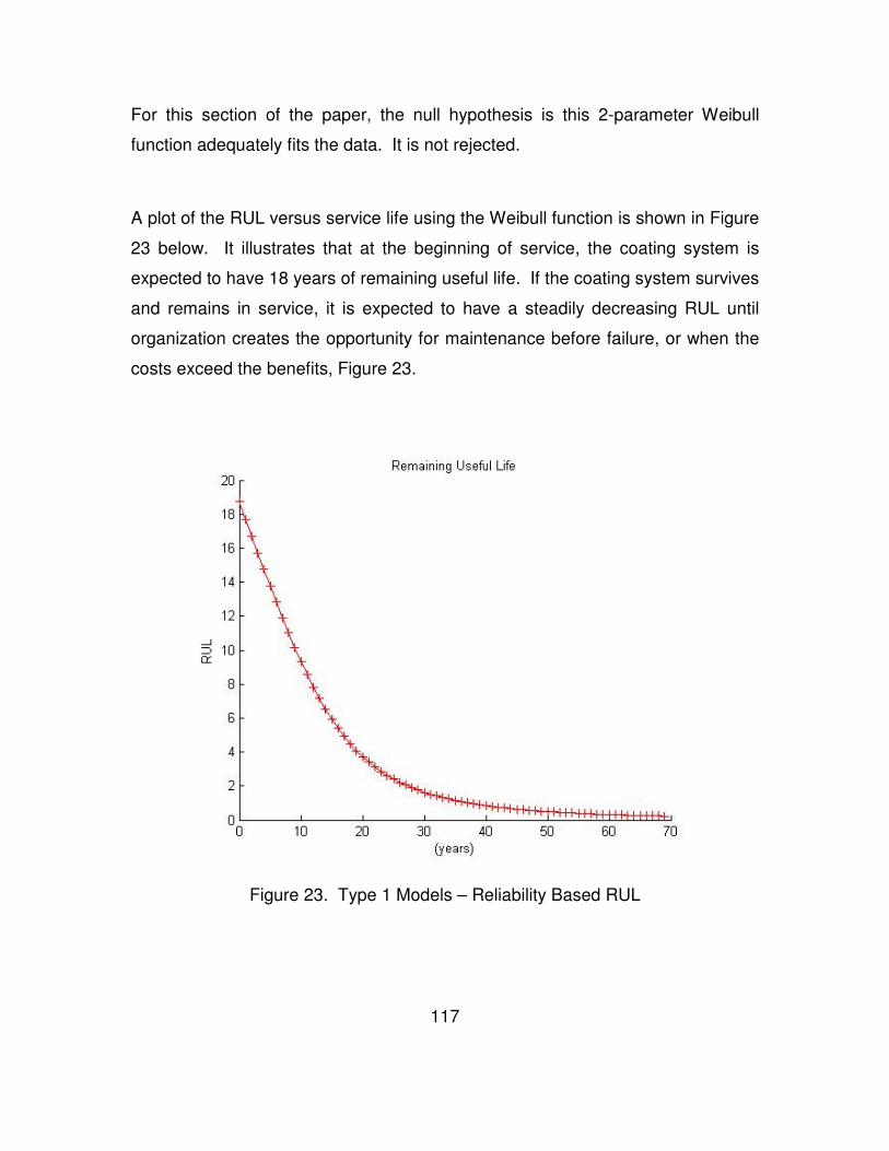
117
For this section of the paper, the null hypothesis is this 2-parameter Weibull
function adequately fits the data. It is not rejected.
A plot of the RUL versus service life using the Weibull function is shown in Figure
23 below. It illustrates that at the beginning of service, the coating system is
expected to have 18 years of remaining useful life. If the coating system survives
and remains in service, it is expected to have a steadily decreasing RUL until
organization creates the opportunity for maintenance before failure, or when the
costs exceed the benefits, Figure 23.
Figure 23. Type 1 Models – Reliability Based RUL

118
4.2.2 Type 2 Cox Proportional Hazards Model
MLE was used to determine the values of the parameters given in Table 7.
Service environment parameter statistics are listed first, and surface preparation
parameter statistics are listed second.
Table 7. Cox PhM Statistics
Statistic Value
covb C 3.3439 −0.1680−0.1680 1.9741 K Beta (β) C−0.92295.5504 K
se C1.82861.4050K z (β/se) C−0.50473.9504 K p-value C0.61380.0001K
‘covb’ describes the variance of the model parameter Beta (β). ‘se’ is the
standard error of (β). ‘z’ is the z-statistic. ‘p-value’ indicates the effect of the
covariate is significant.
Figure 24 illustrates the effects that different service environments and surface
preparation methods have on the hazard rate, and by extension, the life of the
coating system. This plot shows that contaminated service coatings fail at a
faster rate compared to storage service coatings. It also shows that coating

119
systems with grit blast surface preparation fail slower than hand/power tool
surface preparation methods.
Figure 24. Type 2 Models – Cox PhM Cumulative Hazard Rate vs Time
Figure 25 illustrates the reliability of the system for each of the five factors. It
shows that coating substrates prepared with grit blast surface preparation survive
longer than hand/power tool prepared surfaces. It also shows that coating in
storage service environments survive longer than contaminated service
environments.
Figure 26 illustrates the RULs for each of the 4 features shown. The RUL for
service environment 2 were not shown because it performs very similar to
service 1. Local peaks in the data represent some type of activity or change in

120
Figure 25. Type 2 Models – Cox PhM Reliability vs Time
Figure 26. Type 2 Models – Cox PhM Based RUL

121
the field as it was recorded in the data. The results show that late in the coating
service life, there appear to be a number of actions that may represent
maintenance or risk decisions.
4.2.3 Type 3 General Path with Bayesian Updating Model
A linear function, a quadratic function, and an exponential function were fit to the
training data. The average Mean Squared Error (MSE) for each are listed in
Table 8 below. While the exponential function provided a slightly better fit,
parameters from the quadratic function were advanced in the analysis due to
certain complications associated with the exponential function.
The parameters of the quadratic function are listed in Table 9 below. Values in
the ratio are all over 2%, indicating the effects represented by the data and the
parameters of these analyses are component effects, not constant population
effects.
Table 8. Type 3 Models – GPM with Bayesian Mean Squared Error
Model Type MSE
Linear 3.0959
Quadratic 2.3583
Exponential 2.3317
Roy’s Test resulted in a Royston’s statistic p-value of 6.0e-6, well below the
typical p=0.050 threshold for confirming normality. Figure 27 shows degradation
paths for training data. At the top are red asterisks indicating the time of failure,
when the system was found in condition state 4. Degradation paths are

122
dominated by step-changes instead of smooth paths. This result is reasonable
for data collected on components with very long service lives and relatively few
condition states changes.
Table 9. Quadratic Model Parameter Evaluation
Parameter b1 Parameter b2 Parameter b3
Mean (M) 0.0194 -0.3615 1.3825
Std Dev (S) 0.0180 0.1724 0.3092
ratio = S/M 0.9265 -0.4771 0.2236
Figure 28 has two features. First, it identifies the estimated RUL for the specific
components, operating in specific environments and conditions as the blue
asterisks. Second, the red line shows actual failure times. Any separation
between the blue asterisk and the red line, actual failure from the validation data
group, is error within the model. The two values that are less than zero are
typically a result of the model not having enough data, or the item having already
failed. The point with an Actual RUL of approximately 27 had relatively little data.
The point with an Actual RUL of approximately 37 had the failure recorded at a
lower threshold compared to the others; an error with data management. What is
apparent from the figure is that the Estimate RUL values are lower than the
Actual RUL values. When estimates are lower than actual values, the model is
conservative, and more information is needed to reduce the error in the
projection of the RUL.

123
Figure 27. Type 3 Models – GPM With Updating, Degradation Paths
Figure 28. Type 3 Models – GPM With Bayesian Updating RUL

124
4.2.4 Accuracy of Models
The CRA is listed in Table 10 below for each model. It shows that Type 3
prognostics using the General Path Model and Bayesian updating provided the
most accurate results. A Type 3 model with residuals was expected to provide
more accurate results, but did not due to limitations within the residuals
themselves. A Type 2 prognostic model using Cox PhM provides slightly more
accurate results than the Type 1 model for this data on coating systems applied
over substrate prepared using grit blast media. Other PhM factors did not result
in more accurate models. Type 2 MCMC is listed as a consideration, but no CRA
is provided because the approach did not result in informative CRA.
Figure 29 consolidates the results of the four different models. In the Type 1
model, area 1 shows a grouping of several different RUL points. This highlights
the fact that Type 1 models do not represent dimensionality in the data. All
components are evaluated just the same as the average component, regardless
of their specific operating environments and conditions. In contrast, area 2 in the
Type 2 model shows dimensionality in the RUL estimates. Different colors
represent RULs for the average component, operating in specific environments
and conditions. The Type 3 models are the most sensitive and more accurate
compared to the other types of prognostic models. They represent the RUL for
the specific component, operating in its specific environment, under specific
conditions. Figure 29 illustrates the benefit gained from using a maintenance
policy and practices that make use of data with higher dimensionality to improve
the accuracy in estimated RULs. For the Type 3 model with residuals, while it
centers the individual RULs about the red reference line and provides a better fit
to the data with lower mean squared error, Table 10 shows that it results in a
lower cumulative relative accuracy compared to the other Type 3 model.

125
Table 10. Cumulative Relative Accuracy of Prognostic Models
Model CRA
Type 1 – Reliability 0.043
Type 2 – Cox Proportional Hazards
Surface Preparation 1 0.046
Surface Preparation 2 0.022
Storage Service 0.021
Contaminated Service 0.019
Type 2 – Markov Chain Monte Carlo -
Type 3 – GPM w/ Bayesian Updating 0.269
Type 3 – GPM w/ Bayesian & Residuals 0.179

126
Figure 29. Prognostic Model Comparison

127
CHAPTER 5: CONCLUSIONS AND RECOMMENDATIONS
The original scope of this project was to apply prognostic algorithms to a set of
data and, depending on the results, prove they can be used to optimize
equipment maintenance. In due course, research identified some instances and
feedback that indicated otherwise. So it became necessary to expand the scope
and investigate a number of related topics to ensure the following conclusions
are based on facts, evidence, and address different perspectives that influence
the success of prognostics.
On the outset, the major conclusion of this project is that prognostic algorithms
can be used to optimize equipment maintenance. This is proven in Chapter 4.
The secondary conclusion is, if they are not applied correctly, then they are less
likely to provide optimal results. In a traditional sense, optimization is achieved
by minimizing cost and maximizing availability of equipment. However, in
practice, it can only be achieved by simultaneously satisfying objective
requirements and subjective opinions that address the context of optimization for
the individual organization. If the organization does not fully commit to the effort,
adjusting its structure to be more sensitive to affordability and logistic factors that
contribute to maintainability at the plant or SoS levels, and collect and fully
process the right data, then it may be dissatisfied with the results of prognostic
analyses that, today, mostly apply to individual pieces of equipment. The
following discussion continues along these lines and with the top-down, outside-
in approach used throughout the thesis.
There appears to be a relationship between, the size of the organization
efficiency, and the most preferred policy. Smaller organizations tend to be more
centralized, and have fewer constraining influences enabling faster and more
definitive decisions. They are often limited by the amount and quality of historical
128
data, and by the costs associated with implementing and sustaining more
advanced systems. Rapid advancements in computer software and electronic
communications will close many of the gaps between small and large
organizations in the future making a PHM system a more frequent choice.
Larger organizations, in contrast, make decisions more slowly due to the spread
in their infrastructure and processes, and broad communication. While it is wise
for large organizations to make decisions based on input from all of the
stakeholders, it does so at the cost of longer response times that increases
maintenance delays. Small organizations benefit from the fact that sounded
condition alarms can rise to the top and descend in the form of a decision to field
activities very quickly for JIT maintenance, one of the benefits of CBM. Larger
organizations route alarms throughout a network of locations and suppliers, each
step and stop consuming the benefits of JIT maintenance, forcing wider margins
to be designed into the objective technical requirements to compensate for
inefficient logistic and scheduling processes. This project demonstrated how
AHP can be used to select a maintenance policy, or transition to a maintenance
policy, that is best for all stakeholders in a large organization. Once this is done,
the organization can use a smaller structure and a PHM system to localize the
decision process, enabling faster and for more precise maintenance scheduling
and execution. This project recommends using AHP to shrink the size of the
maintenance planning process and decision space.
Most of the literature that was reviewed provided incomplete instruction on life
cycle maintenance. While they provided an outline of different milestone-
activities for life cycle management, Figure 3, and directed subordinate activities
to use advanced methods such a predictive and proactive maintenance, for in-
service systems they did little to explain how to transition to using advanced
policies. They did little to explain how to integrate important considerations into
the decision making process. This project introduces a novel structure, Figure 1,
and recommends larger organizations use it as a guide when designing

129
maintenance plans for new equipment, or when managing maintenance plans for
in-service equipment. The figure standardizes the taxonomy, highlighting major
considerations needed to make decisions and transition between policies. This
project recommends connecting all systems through a PHM system.
This project concludes that AHP is the most practical method for ensuring
Affordable System Operational Effectiveness considerations are used to manage
the trade space between cost and performance. While other methods exist, they
are either less accurate, doubted, too complicated to explain to at both the
mechanic and senior management levels, or take a long time to build, train, and
validate. AHP appears to strike the right balance between comprehensive
requirements of management, accuracy, fidelity, and usefulness. It comes along
with tools that help an organization identify critical criteria and measure the
values they need to change to transition between maintenance policies. This
project recommends using APH exclusively, or using AHP while more advanced
fuzzy or neural models are developed.
The results, conclusions, and recommendations of this project are neutral when it
comes to preference for a particular maintenance policy. It concludes, rather,
that the important part is that a comprehensive set of requirements, criteria, and
input be involved in the policy selection process. It is equally important to employ
a standard and repeatable method such as AHP, and ensure it is conducted
consistently by experienced facilitators, specifically trained in the method, and
knowledgeable about related technical and procedural matters.
Concerning the data on the paint coating system used in the prognostic
analyses, this project concludes that the use of categorical variables and long
periods of time between assessments resulted in low accuracy for even the best
performing prognostic model. This is a severe weakness of the assessment
program for that system. Categorical variables can easily and immediately be

130
offset by frequent readings of ordinal variables, or continuous data collected by
sensors. The results in Chapter 4 indicate that, in this case, the costs for
developing sensors are far outweighed by the benefits of lower total ownership
costs. Fielding sensors that collect continuous data is recommended.
Based on the data that were used and the prognostic methods involved, this
project concludes that a GPM with Bayesian Updating will provide the most
accurate prediction of the RUL and optimal maintenance scheduling for this paint
coating system. If changes are made to the way the data are collected, then a
GPM with Bayesian Updating and Residuals may provide the most accurate
results. It also finds that continuous monitoring and other prognostic models, and
diagnostic models by extension, provide useful information when examining
different factors in the data, performing FMECA, and doing risk analysis. This
project recommends employing a PHM system designed to build and report the
results of several different kinds of prognostic and diagnostic models.
The results of the GPM with Bayesian Updating analyses were used to calculate
the repair costs for Predictive and Proactive policies used in the AHP algorithm.
The results of AHP analyses indicate that policies that use prognostic algorithms
are the most preferred. Further, analyses indicate that the criteria are robust and
significant changes are required to change the order of preferred policies. If
improvements in data collection are not made and sensors not employed, then
the state-of-the-art for this system resides somewhere between the
Predeterminative and Predictive Policies. In conclusion, it is recommended that
both AHP and prognostic models be used to optimize maintenance for this paint
coating system.

131
CHAPTER 6: FUTURE WORK
Parametric Censoring of Data. In Section 2.6.1.6.1 it was explained that
parametric methods provide the most accurate estimate of ToF for interval
censored data. The results of these analyses were calculated using the mid-
point method. RUL projections will be more accurate if parametric methods are
used to estimate ToF, and greatly improved if continuous data are used.
Interaction Effects and Combinations of Factors in AHP. The calculations used
in these analyses evaluated the influence of each factor individually. This project
acknowledges the potential enhanced benefits of AHP based on interaction
effects and different combinations of factors.
Applicability to Other Systems, Organizational Structures, and Other Areas.
This thesis is organized so it can be used as a universal instruction – just follow
the steps, incorporate lessons learned, and watch out for known pitfalls. It is
universal in the sense that it can be scaled up or down according to the structure
and size of the organization, or the specific application. These methods are
applicable to large SoS or individual components. They apply to all types of
active and passive systems including computers, electrical systems, piping and
pumps, air handling systems, structural systems, drive systems, braking
systems, automobiles, bicycles, aircraft, ships, buildings, iPads, chainsaws,
paper mills, heart defibrillator manufacturing plants, soda bottling companies, etc.
With highly complex systems like robotics, drones, and autonomous vehicles on
the rise, Bosco’s model and AHP can be tailored and applied to meet those
specific application. For example, prognostic models can be used to project the
time of arrival or collision, and provide information to guidance systems on

132
course corrections. As of 2017, it appears that a new space race has begun, so
there is a demand for simulation and avionics work.
Prognostic algorithms have a broad array of applications beyond equipment
maintenance; modeling weather patters, financial market projections, and
biomedical applications are just a few. Forecasting future performance and
behavior, and taking proactive action to ensure safety or maximize advantage will
always be needed in these areas.
Lack of and quality of historical data will always be constraints. In the strongest
possible way, this paper recommends performing a robust FMECA, using
sensors to frequently collect data using continuous variables, and a PHM system
to store, analyze, and manage the data. If any one of these are missing, the
organization will probably be forced to make broad decisions based on limited
data and inaccurate analysis.
To complete this project, the discussion is returned to the opening statements.
This work finds that component-level CbM is applicable at the plant-level, only if
plant-level requirements and processes are designed into the component-level
life cycle management system.

133
LIST OF REFERENCES

134
[1] INCOSE, Systems Engineering Handbook: A Guide for Systems Life Cycle
Processes and Activities, New York: John Wiley & Sons, 2015.
[2] C. Ebeling, An Introduction to Reliability and Maintainability Engineering,
Long Grove: Waveland Press, Inc., 2010.
[3] ReliaSoft Corporation, "Weibull.com," January 2011. [Online]. Available:
http://www.weibull.com/hotwire/issue119/hottopics119.htm. [Accessed
12/17/2016 December 2016].
[4] F. Khan, "Equipment reliability a life-cycle approach," Engineering
Management Journal, vol. 11, no. 3, pp. 127-135, June 2001.
[5] A. Carter, "Better Buying Power: Mandate for Restoring Affordability and
Productivity in Defense Spending," DoD, Washington, DC, 2010.
[6] "Defense Acquisition University," Defense Acquisition University, 17
December 2016. [Online]. Available:
https://dap.dau.mil/aap/pages/qdetails.aspx?cgiSubjectAreaID=43&cgiQue
stionID=118392. [Accessed 17 December 2016].
[7] S. Ding and S. Kamaruddin, "Maintenance policy optimization-literature
review and directions," The International Journal of Advanced
Manufacturing Technology, vol. 76, no. 5, pp. 1263-1283, 2015.
[8] W. Tiddens, A. Braaksma and T. Tinga, "The adoption of prognostic
technologies in maintenance decision making: a multiple case study," in
The Fourth International Conference on Through-life Engineering
Services, 2015.
[9] K. Khazraei and J. Deuse, "A strategic standpoint on maintenance
taxonomy," Journal of Facility Management, vol. 9, no. 2, pp. 96-113,
2011.
[10] J. Moubray, Reliability-centered Maintenance, 2nd Ed., New York:
Industrial Press Inc., 1997.

135
[11] J. Koochaki, J. Bokhorst, H. Wortmann and W. Klingenberg, "Condition
based maintenance in the context of opportunistic maintenance,"
International Journal of Production Research, vol. 50, no. 23, pp. 6918-
6929, 2012.
[12] J. Gao, D. Quass and Y. Ng, "Selective-Splitting and Cache-Maintenance
Algorithms for Associative-Client Caches," Distributed and Parallel
Databases, vol. 16, no. 1, pp. 5-43, 2004.
[13] J. Mitchell, "Five to ten year vision for CBM," in paper presented at the
ATP Fall Meeting - Condition Based Maintenance Workshop, Atlanta,
1998.
[14] S. Yang, "A condition-based failure-prediction and processing-scheme for
preventive maintenance," IEEE Transactions on Reliability, vol. 52, no. 3,
pp. 373-383, 2003.
[15] L. Wang, J. Chu and J. Wu, "Selection of optimum maintenance strategies
based on a fuzzy analytic hierarchy process," International Journal of
Production Economics, vol. 107, no. 1, pp. 151-163, 2007.
[16] P. Tsai, Y. Lin, Y.-Z. Ou, E. Chy and J. Liu, "A Framework for Fusion of
Human Sensor and Physical Sensor Data," IEEE Transaction fon
Systems, Man, and Cybernetics: Systems, vol. 44, no. 9, pp. 1248-1261,
2014.
[17] G. Waeyenbergh, L. Pintelon and L. Gelders, "A stepping stone towards
knowledge based maintenance," South African Journal of Industrial
Engineering, vol. 12, no. 2, pp. 61-81, 2001.
[18] M. Organ, T. Whitehead and M. Evans, "Availability-based maintenance
within an asset management programme," Journal of Quality in
Maintenance, vol. 3, no. 4, pp. 221-232, 1997.

136
[19] Y. Tsai, K. Wang and L. Tsai, "A study of availability-centered preventive
maintenance for multi-component systems," Reliability Engineering and
Systems Safety, vol. 84, no. 3, pp. 261-270, 2004.
[20] G. Waeyenbergh and L. Pintelon, "A framework for maintenance concept
development," International Journal of Production Economics, vol. 77, no.
3, pp. 299-313, 2002.
[21] L. Krishnasamy, F. Khan and M. Haddara, "Development of a risk-based
maintenance (RBM) strategy for a power-generating plant," Journal of
Loss Prevention in the Process Industries, vol. 18, pp. 69-81, 2005.
[22] J. BareiB, P. Buck, B. Matschecko, A. Jovanovic, D. Balos and M.
Perunicic, "RIMAP demonstration project. Risk-based life management of
piping system in power plant Heilbronn," International Journal of Pressure
Vessels and Piping, vol. 81, pp. 807-813, 2004.
[23] K. Fujiyama, S. Nagai, Y. Akikuni, T. Fujiwara, K. Furuya, S. Matsumoto,
K. Takagi and T. Kawabata, "Risk-based inspection and maintenance
systems for steam turbines," International Journal of Pressure Vessels and
Piping, vol. 81, pp. 825-835, 2004.
[24] NASA, "NASA Public Web Page," September 2008. [Online]. Available:
http://www.hq.nasa.gov/office/codej/codejx/Assets/Docs/NASARCMGuide.
pdf. [Accessed 22 December 2016].
[25] U. DoE, "Department of Energy Public Web Page," August 2010. [Online].
Available:
https://energy.gov/sites/prod/files/2013/10/f3/omguide_complete.pdf.
[Accessed 22 December 2016].
[26] C. Carlson, Effective FMEAs, Hoboken: Wiley, 2012.
[27] I. Ahuja and J. Khamba, "Total productive maintenance: literature review
and directions," International Journal of Quality & Reliability Management,
vol. 25, no. 7, pp. 709-756, 2008.

137
[28] J. Majumdar and M. Manohar, "Implementing TPM programme as a TQM
tool in Indian manufacturing industries," Asian Journal on Quality, vol. 13,
no. 2, pp. 185-198, 2012.
[29] F. Ireland and B. Dale, "A study of total productive maintenance
implementation," Journal of Quality in Maintenance Engineering, vol. 7, no.
3, pp. 183-192, 2001.
[30] H. Steinbacher and N. Steinbacher, TPM for America, Portland:
Productivity Press, 1993.
[31] R. Davis, "Making TPM a part of factory life," Works Management, vol. 49,
no. 7, pp. 16-17, 1996.
[32] U. S. Government, Defense Acquisition Guidebook, 2016.
[33] J. Bobinis and T. Herald, "An enterprise framework for operationally
effective system of systems design," Journal of Enterprise Architecture,
vol. 8, no. 2, pp. 60-75, 2012.
[34] T. Markeset and U. Kumar, "Design and development of product support
and maintenance concepts for industrial systems," Journal of Quality in
Maintenance Engineering, vol. 9, no. 4, pp. 376-392, 2003.
[35] G. A. Office, "Setting Requirements Differently Could Reduce Weapons
Systems' Total Ownership Costs," United States GAO, Washington, DC,
2003.
[36] J. Bobinis, C. Garrison, J. Haimowitz, J. Klingberg, T. Mitchell and P.
Tuttle, "Affordability Considerations: Cost Effective Capability," INCOSE
Affordability Working Group, 2013.
[37] A. Jardine and A. Tsang, Maintenance, Replacement, and Reliability, New
York: Taylor and Francis Group, 2006.
[38] L. Crow, "Methods for Reducing the Cost to Maintain a Fleet of Repairable
Systems," in Annual Reliability and Maintainability Symposium, 2003.
138
[39] N. Saqib and M. Siddiqi, "Thresholds and goals for safety performance
indicators for nuclear power plants," Reliability Engineering and System
Safety, vol. 87, pp. 275-286, 2005.
[40] P. O'Connor and A. Kleyner, Practical Reliability Engineering, West
Sussex: Wiley & Sons, 2012.
[41] W. Geradas, "The EUT maintenance model," International Journal of
Production Economics, vol. 24, no. 3, pp. 209-216, 1992.
[42] K. Marais and J. Saleh, "Beyond its cost, the value of maintenance; an
analytical framework for capturing its net present value," Reliability
Engineering System Safety, vol. 94, no. 2, pp. 644-657, 2009.
[43] B. Bevilacqua and M. Braglia, "The analytic process applied to
maintenance strategy selection," Reliability Engineering and System
Safety, vol. 70, no. 1, pp. 71-83, 2000.
[44] A. Labib, "World-class maintenance using a computerised maintenance
management system," Journal of Quality in Maintenance Engineering, vol.
4, no. 1, pp. 66-75, 1998.
[45] O. Fernandez and A. Labib, "A decision support maintenance
management system Development and implementation," International
Journal of Quality & Reliability Management, vol. 20, no. 8, pp. 965-979,
2003.
[46] J. Khalil, S. Saad, N. Gindy and K. MacKechnie, "A maintenance policy
selection tool for industrial machine parts," International Federation for
Information Processing, vol. 159, pp. 431-440, 2005.
[47] S. Gupta, J. Maiti, R. Kumar and U. Kumar, "A control chart guided
maintenance policy selection," International Journal of Mining,
Reclamation and Environment, vol. 23, no. 3, pp. 216-226, 2009.

139
[48] M. Samrout, E. Chatelet, R. Kouta and N. Chebbo, "Optimization of
maintenance policy using the proportional hazard model," Reliability
Engineering and System Safety, vol. 94, pp. 44-52, 2009.
[49] S. Marorell, A. Sanchez and V. Serradell, "Age-dependent reliability model
considering effects of maintenance and working conditions," Reliability
Engineering and System Safety, vol. 64, pp. 19-31, 1999.
[50] G. Waeyenbergh and L. Pintelon, "A framework for maintenance concept
development," International Journal of Production Economics, vol. 77, pp.
299-313, 2002.
[51] G. Waeyenbergh and L. Pintelon, "Maintenance concept development: A
case study," International Journal of Production Economics, vol. 89, pp.
395-405, 2004.
[52] G. Waeyenbergh and L. Pintelon, "CIBOCOF: A framework for industrial
maintenance concept development," International Journal of Production
Economics, vol. 121, pp. 633-640, 2009.
[53] M. Braglia, M. Frosolini and R. Montanari, "Fuzzy criticality assessment
model for failure modes and effects analysis," International Journal of
Quality & Reliability Management, vol. 20, no. 4, pp. 503-524, 2003.
[54] D. Li and J. Gao, "Study and application of Reliability-centered
Maintenance considering Radical Maintenance," Journal of Loss
Prevention in the Process Industries, vol. 23, pp. 622-629, 2010.
[55] E. Triantaphyllou, B. Kovalerchuk, L. Mann and G. Knapp, "Determining
the most important criteria in maintenance decision making," Journal of
Quality in Maintenance Engineering, vol. 3, no. 1, pp. 16-28, 1997.
[56] A. Garg and S. Deshmukh, "Maintenance management: literature review
and directions," Journal of Quality in Maintenance Engineering, vol. 12, no.
3, pp. 205-238, 2006.

140
[57] A. Sharma, G. Yadava and S. Deshmukh, "A literature review and future
perspectives on maintenance optimization," Journal of Quality in
Maintenance Engineering, vol. 17, no. 1, pp. 5-25, 2011.
[58] L. Swanson, "Linking maintenance strategies to performance,"
International Journal of Production Economics, vol. 70, pp. 237-244, 2001.
[59] J. Koochaki, J. Bokhorst, H. Wortmann and W. Klingenberg, "The
influence of condition-based maintenance on workforce planning and
maintenance scheduling," International Journal of Production Research,
vol. 51, no. 8, pp. 2339-2351, 2013.
[60] J. Koochaki, J. Veldman and J. Wortmann, "Literature survey on condition
based maintenance within the process industry," in 21st Congress of
COndition Monitoring and DIagnostic Engineering Management, 2008.
[61] X. Zheng and N. Fard, "Hazard-rate tolerance method for an opportunistic-
replacement policy," IEEE Transactions on Reliability, vol. 41, no. 1, pp.
13-20, 1992.
[62] Y. Peng, M. Dong and M. Zuo, "Current status of machine prognostics in
condition-based maintenance: a review," International Journal of
Advanced Manufacturing Technologies, vol. 50, pp. 297-313, 2010.
[63] J. Coble, P. Ramuhalli, L. Bond, J. Hines and Upadhyaya, "A Review of
Prognostics and Health Management Applications in Nuclear Power
Plants," International Journal of Prognostics and Health Management, vol.
6, no. 3, pp. 1-22, 2015.
[64] C. Jensen, T. Pedersen and C. Thomsen, Multidimensional Databases
and Data Warehousing, San Rafael: Morgan & Claypool, 2010.
[65] M. Kaya and R. Alhajj, "Development of multidimensional academic
information networks with a novel cube based modeling method,"
Information Sciences, vol. 265, pp. 211-224, 2014.

141
[66] A. Tamhane and D. Dunlop, Statistics and Data Analysis from Elementary
to Intermediate, Upper Saddle River: Prentice Hall, 2000.
[67] J. Hellerstein, "Quantitative Data Cleaning for Large Databases," United
Nations Economic Commission for Europe, Berkeley, 2008.
[68] S. Fienberg, "Randomization and Social Affairs: The 1970 Draft Lottery,"
Science, vol. 171, no. 3968, pp. 255-261, 1971.
[69] G. Afendras and M. Marianthi, "UTK ONESEARCH," 10 November 2015.
[Online]. Available: http://utk-
almaprimo.hosted.exlibrisgroup.com/primo_library/. [Accessed 31
December 2016].
[70] D. Montgomery, G. Runger and N. Hubele, Engineering Statistics,
Hoboken: John Wiley & Sons, Inc., 2011.
[71] P. Allison, Survival Analysis Using SAS, Cary: SAS Institute Inc., 2010.
[72] R. Singh and D. Totawattage, "The Statistical Analysis of Interval-
Censored Failure Time Data with Applications," Open Journal of Statistics,
vol. 3, pp. 155-166, 2013.
[73] B. Turnbull, "The Empirical Distribution Function with Arbitrarily Grouped,
Censored and Truncated Data," Journal of the Royal Statistical Society,
vol. 38, no. 3, pp. 290-295, 1976.
[74] K. Ramachandran, K. Fathi and B. Rao, "Recent Trends in Systems
Performance Monitoring & Failure Diagnostics," in IEEE International
Conference on Industrial Engineering and Engineering Management
(IEEM), Macao, 2010.
[75] A. Wald, "Sequential Tests of Statistical Hypotheses," The Annals of
Mathematical Statistics, vol. 16, no. 2, pp. 117-186, 1945.
[76] Q. Yang, "Case Western Reserve University," 2004. [Online]. Available:
http://rave.ohiolink.edu/etdc/view?acc_num=case1080246972. [Accessed
1 January 2017].

142
[77] T. Dijkstra, "Ridge regression and its degrees of freedom," Quality &
Quantity, vol. 48, no. 6, pp. 3185-3193, 2014.
[78] A. Sen and M. Srivastava, Regression Analysis, New York: Springer-
Verlag, 1990.
[79] V. Centner and D. Massart, "Optimization in locally weighted regression,"
Analytical Chemistry, vol. 70, no. 19, pp. 4206-4211, 1998.
[80] R. Rengaswamy and V. Venkatasubramanian, "A fast training neural
network and its updation for incipient fault detection and diagnosis,"
Computers and Chemical Engineering, vol. 24, pp. 431-437, 2000.
[81] J. Coble and J. Hines, "Prognostic Algorithm Categorization with PHM
Challenge Application," in International Conference on Prognostics and
Health Management, Denver, 2008.
[82] G. Sims, "Physics of Failure," Science, vol. 201, p. 435, 1964.
[83] R. Faynman, "feynman," 1986. [Online]. Available:
http://www.feynman.com/. [Accessed 2 January 2017].
[84] S. Bertsch, The theory that would not die, New Haven: Yale, 2011.
[85] J. Martin, S. Saunders and F. W. J. Floyd, "Methodologies for predicting
the service lives of coating systems," National Institute of Standards and
Technology, Springfield, VA, 1994.
[86] E. Schmitt, "Development and Deployment of a High Throughput Exterior
Durability Program for Architectural Paint Coatings," in Service Life
Prediction of Polymeric Materials Global Perspectives, New York,
Springer, 2009, pp. 397-404.
[87] ASTM, ASTM D610 Standard Practice for Evaluating Degree of Rusting
on Painted Steel Surfaces, West Conshohocken: ASTM International,
2012.
[88] ASTM, ASTM D714 Standard Test Method for Evaluating Degree of
Blistering of Paints, West Conshohocken: ASTM International, 2009.

143
[89] H. Wang, "Comparison of the Goodness-of-Fit Tests; the Pearson Chi-
Squared and Kolmogorov-Smirnov Tests," Ling Tung University, Taiwan,
2009.
[90] M. Todinov, Reliability and Risk Models Setting Reliability Requirements,
West Sussex: Wiley, 2005.
[91] J. Coble and W. Hines, "Applying the General Path Model to Estimation of
Remaining Useful Life," International Journal of Prognostics and Health
Management, vol. 2, no. 1, pp. 72-84, 2011.
[92] R. Sharma, D. Kumar and P. Kumar, "FLM to select suitable maintenance
strategy in process industries using MISO model," Journal of Quality
Maintenance Engineering, vol. 15, no. 6, pp. 1129-1140, 2005.
[93] J. Koochaki, J. Bokhorst, H. Wortmann and W. Klingenberg, "Condition
based maintenance in the context of opportunistic maintenance,"
International Journal of Production Research, vol. 50, no. 23, pp. 6918-
6929, 2012.
[94] B. Rao, "Educational needs in condition monitoring and diagnostic
engineering management (COMADEM)," Journal of Measurement and
Control, vol. 19, no. 10, pp. 306-309, 1987.
[95] K. Goode, B. Roylance and J. Moore, "Development of model to predict
condition monitoring interval times," Iron making and steel making, vol. 27,
pp. 63-68, 2000.
[96] J. Coble, J.W. Hines, "Applying the General Path Model to Estimation of
Remaining Useful Life," International Journal of Prognostics and Health
Management, ISSN 2153-2648, 007, 2011

144
APPENDICES

145
APPENDIX A - TABLES
Table 11. Literature Review of Topics
Topic ID Maintenance Topic
A Optimization models
B Techniques
C Scheduling
D Performance measurement
E Information system
F Policies
Source: Garg et al., "Maintenance management: literature review and directions”, 2006

146
Table 12. Literature Review of Topic Publishing By Year
Year
ID 20
04
-20
06
20
03
20
02
20
01
20
00
19
99
19
98
19
97
19
96
19
95
Ea
rlie
r
To
pic
To
tal
A Quantity 3 7 5 1 5 1 3 1 - - 1 27
B Quantity 6 9 8 15 5 7 3 16 2 - 2 73 C Quantity 1 1 2 2 2 1 - - - - - 9 D Quantity 3 4 1 3 1 3 3 2 1 2 - 23 E Quantity 1 - 1 - - 3 - - 1 - - 6 F Quantity 2 1 5 4 1 1 2 1 1 - 1 19 Annual Total
16 22 22 25 14 16 11 20 5 2 4 157
26 �
24 �
22
20
18 �
16 � � �
14
12 �
10
8
6 �
4 �
2 � �
0
Source: Garg et al., "Maintenance management: literature review and directions”, 2006

147
Table 13. Literature Review, Quantity of Publishing By Year
Year
Area Sub Area
200
4-2
006
200
3
200
2
200
1
200
0
199
9
199
8
199
7
199
6
199
5
Earlie
r
Sub-T
ota
l
To
pic
Tota
l
A Maintenance Optimization Models 27 A.1 Bayesian 1 1 - - - - - - - - - 2 A.2 MILP – Mixed Integer Linear Programming - 1 - - - - - - - - - 1 A.3 MCDM – Multi Criteria Decision Making - 1 - - - - - 1 - - - 2 A.4 Fuzzy Linguistic - 1 - 1 - - - - - - - 2 A.5 Galbraith - 1 - - - - - - - - - 1 A.6 MAIC – Materially per Apparecchiature de Impiariti Chemiei - - 1 - - - - - - - - 1 A.7 Simulation - - 2 - 1 - - - - - 1 4 A.8 Markovian Deterioration - 2 1 - 1 - - - - - - 4 A.9 AHP – Analytic Hierarchy Process - - - - 1 - 1 - - - - 2 A.10 Petri Nets - - - - - - 1 - - - - - 1 A.11 Maintenance Organization Modeling 1 - - - 1 - - - - - - 2 A.12 Miscellaneous 1 - 1 - 1 - 2 - - - - 5 ‘A’ Sub-Totals 3 7 5 1 5 1 3 1 - - 1 27
B Maintenance Techniques 73 B.1 PM – Preventive Maintenance 3 4 4 5 2 1 1 1 - - - 21 B.2 CBM – Condition Based Maintenance 1 - 2 1 - 2 - - - - - 6 B.3 TPM – Total Productive Maintenance 1 - - 7 2 1 - - - - - 11 B.4 CMMS – Computerized Maintenance Management Systems - 1 - 1 - 1 1 14 2 - - 20 B.5 RCM – Reliability Centered Maintenance - 2 - 1 1 - 1 - - - - 5 B.6 Predictive Maintenance - 1 - - - 1 - - - - 2 4 B.7 Outsourcing 1 - - - - 1 - 1 - - - 3 B.8 ECM – Effectiveness-Centered Maintenance - - 1 - - - - - - - - 1 B.9 SMM – Strategic Maintenance Management - - 1 - - - - - - - - 1 B.10 RBM – Risk-Based Maintenance - 1 - - - - - - - - - 1 ‘B’ Sub-Totals 6 9 8 15 5 7 3 16 2 - 2 73
C Maintenance Scheduling 9 C.1 Techniques C.1.1 CBM 1 1 - - - - - - - - - 2 C.1.2 Predictive - - 1 - - - - - - - - 1 C.1.3 PM - - - 1 1 - - - - - - 2 C.2 Wear-Out Components - - 1 - - - - - - - - 1 C.3 Repair Rate Modifying Activities - - - 1 - - - - - - - 1 C.4 Combining Production and Maintenance - - - - 1 - - - - - - 1 C.5 Maintenance Personnel - - - - - 1 - - - - - 1 ‘C’ Sub-Totals 1 1 2 2 2 1 - - - - - 9
Source: Garg et al., "Maintenance management: literature review and directions”, 2006

148
Table 13. Continued – Literature Review, Quantity of Publishing By Year
Year
Area Sub Area
200
4-2
006
200
3
200
2
200
1
200
0
199
9
199
8
199
7
199
6
199
5
Earlie
r
Sub-T
ota
l
To
pic
Tota
l
D Maintenance Performance Measurement 23 D.1 Techniques D.1.1 Various Models - - - - - 1 - 1 - - - 2 D.1.2 VBM – Vibration-Based Maintenance 1 - - - - - - - - - - 1 D.1.3 BSC – Balanced Score Card - 1 - - - - 1 - - - - 2 D.1.4 QFD – Quality Function Deployment - - - 1 - - - - - - - 1 D.1.5 MIS – Maintenance Information Systems - - - - - - 1 - - - - 1 D.1.6 TMM – Total Maintenance Management - - - - - - - - - 1 - 1 D.1.7 System Audit Approach - - - - - 1 - - - 1 - 2 D.1.8 Maintenance Productivity Index - - - - 1 - - - - - - 1 D.2 Overall Equipment / Craft Effectiveness - 2 - 1 - - 1 - - - - 4 D.3 Relation With Maintenance Strategy 2 - - 1 - - - - - - - 3 D.4 Effect of Failure on Effectiveness - - - - - 1 - - - - - 1 D.5 Miscellaneous - 1 1 - - - - 1 1 - - 4 ‘D’ Sub-Totals 3 4 1 3 1 3 3 2 1 2 - 23
E Maintenance Information System 6 E.1 Opportunity Created by IT - - - - - 1 - - - - - 1 E.2 Computerized Data Based Info System to Reduce MTTR / MTBF - - - - - - - - 1 - - 1
E.3 Development of DSS (Decision Support Systems) in Maintenance Planning
- - - - - 1 - - - - - 1
E.4 Miscellaneous 1 - 1 - - 1 - - - - - 3 ‘E’ Sub-Totals 1 - 1 - - 3 - - 1 - - 6
F Maintenance Policies 19 F.1 Maintenance Integration - - 1 2 1 1 - - - - - 5 F.2 Emerging Maintenance Concepts F.2.1 EMQ Determination in Imperfect PM - - - 1 - - 1 - - - - 2 F.2.2 Simulation in Maintenance 1 - 1 - - - - - - - - 2 F.2.3 Customized Maintenance Concept - - 1 - - - - - - - - 1 F.2.4 Object-Oriented Maintenance Management - 1 - - - - - - - - - 1 F.3 New Ideas 1 - - 1 - - 1 - - - - 3 F.4 Miscellaneous (Includes review papers) - - 2 - - - - 1 1 - 1 5 ‘F’ Sub-Totals 2 1 5 4 1 1 2 1 1 - 1 19
Totals 16 22 22 25 14 16 11 20 5 2 4 157

149
Table 14. Literature Review on Optimization Criteria Reported
Researchers Optimal Criteria Optimal Function
Labib et al. (1998) Reliability/Maintainability TPM
Dinesh Kumar (1999) Maintenance Cost Availability
Ben-Daya and Alghamdi (2000) Availability Optimal Degradation
Marseguerra et al. (2002) Reliability Level for Preventive Maint.
Goel et al. (2003) Maintenance Cost Equipment / Manpower
Mirghani (2003) Cost/Availability Planned Maintenance Job
Liu and Yu (2004) Availability Efficient Plant Maintenance
Moya (2004) Failure Rate Preventive Maint. Prog
Mathew (2004) Availability/Reliability Spare Parts Req.; Man-Hour
Eti et al. (2005) Failure Rate Maintenance Scheduling
Kianfar (2005) Maintenance Cost Discounted Profit
Pongpech et al. (2006) Failure Rate Equipment Availability
Ho and Silva (2006) Optimal Sequence Reliability
Nahas et al. (2008) Failure Probability Reliability
Cadini et al. (2009) Reliability Replacement on Failure;
Preventive Replacement
Source: Sharma et al., "A literature review and future perspectives on maintenance optimization," 2011
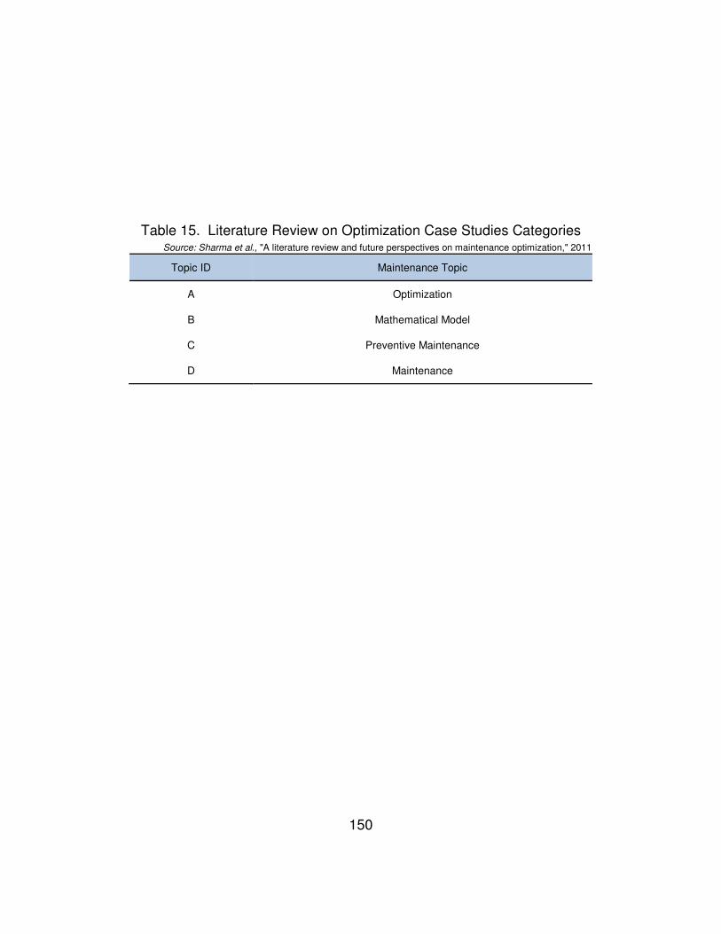
150
Table 15. Literature Review on Optimization Case Studies Categories
Topic ID Maintenance Topic
A Optimization
B Mathematical Model
C Preventive Maintenance
D Maintenance
Source: Sharma et al., "A literature review and future perspectives on maintenance optimization," 2011

151
Table 16. Literature Review on Optimization Case Studies
Year
ID 20
07
20
06
20
05
20
04
20
03
20
02
20
01
20
00
19
99
19
98
19
97
To
pic
To
tal
A Quantity 1 2 4 3 1 1 2 1 1 1 1 18
B Quantity - - 1 3 1 1 1 3 2 2 - 14
C Quantity - 1 1 4 1 2 2 - - 1 - 12
D Quantity - 2 3 1 2 1 1 2 1 - 2 15
Annual Total
1 5 9 11 5 5 6 6 4 4 3
12
10 �
8 �
6 � �
4 � � � � �
2 �
0 �
Source: Sharma et al., "A literature review and future perspectives on maintenance optimization," 2011

152
Table 17. PCA and PLS Applications for Fault Diagnostics
Sources Method Application
Dunia et al. PCA Sensor fault detection, identification, reconstruction
Qin and Li PCA Sensor fault detection, identification, reconstruction
Dunia and Qin PCA Fault subspace for process and sensor fault detection
Qin PLS Recursive updating to account for time-varying
Li et al. PCA Recursive updating to account for time-varying
Source: Yang, http://rave.ohiolink.edu/etdc/view?acc_num=case1080246972, 2004
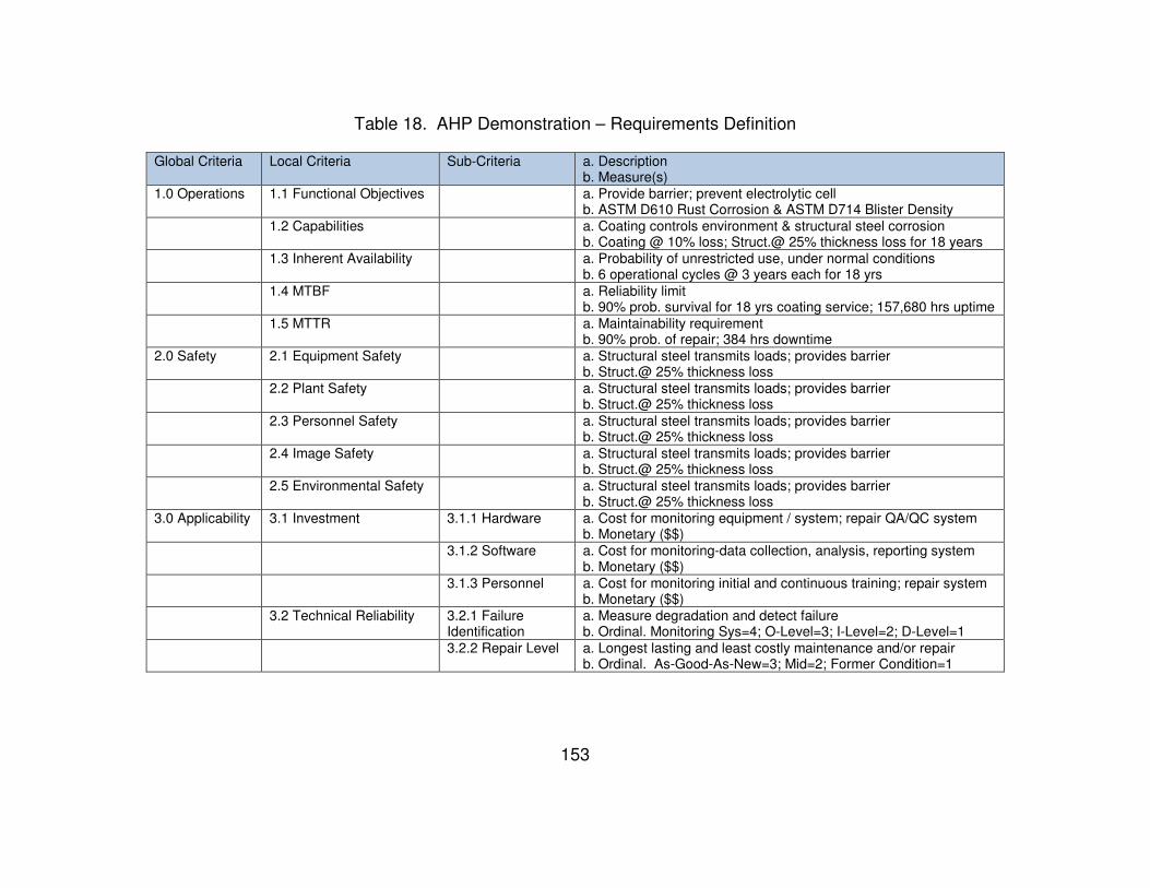
153
Table 18. AHP Demonstration – Requirements Definition
Global Criteria Local Criteria Sub-Criteria a. Description b. Measure(s)
1.0 Operations 1.1 Functional Objectives a. Provide barrier; prevent electrolytic cell b. ASTM D610 Rust Corrosion & ASTM D714 Blister Density
1.2 Capabilities a. Coating controls environment & structural steel corrosion b. Coating @ 10% loss; Struct.@ 25% thickness loss for 18 years
1.3 Inherent Availability a. Probability of unrestricted use, under normal conditions b. 6 operational cycles @ 3 years each for 18 yrs
1.4 MTBF a. Reliability limit b. 90% prob. survival for 18 yrs coating service; 157,680 hrs uptime
1.5 MTTR a. Maintainability requirement b. 90% prob. of repair; 384 hrs downtime
2.0 Safety 2.1 Equipment Safety a. Structural steel transmits loads; provides barrier b. Struct.@ 25% thickness loss
2.2 Plant Safety a. Structural steel transmits loads; provides barrier b. Struct.@ 25% thickness loss
2.3 Personnel Safety a. Structural steel transmits loads; provides barrier b. Struct.@ 25% thickness loss
2.4 Image Safety a. Structural steel transmits loads; provides barrier b. Struct.@ 25% thickness loss
2.5 Environmental Safety a. Structural steel transmits loads; provides barrier b. Struct.@ 25% thickness loss
3.0 Applicability 3.1 Investment 3.1.1 Hardware a. Cost for monitoring equipment / system; repair QA/QC system b. Monetary ($$)
3.1.2 Software a. Cost for monitoring-data collection, analysis, reporting system b. Monetary ($$)
3.1.3 Personnel a. Cost for monitoring initial and continuous training; repair system b. Monetary ($$)
3.2 Technical Reliability 3.2.1 Failure Identification
a. Measure degradation and detect failure b. Ordinal. Monitoring Sys=4; O-Level=3; I-Level=2; D-Level=1
3.2.2 Repair Level a. Longest lasting and least costly maintenance and/or repair b. Ordinal. As-Good-As-New=3; Mid=2; Former Condition=1

154
Table 18. Continued - AHP Demonstration – Requirements Definition
Global Criteria Local Criteria Sub-Criteria a. Description b. Measures
4.0 Added Value
4.1 TPM Feedback Maturity
a. TPM provides best results to organization; state-of-the-art b. Ordinal. Highest and best=5; Lowest=1
4.2 PHM Processing Maturity
a. PHM provides best results to organization; state-of-the-art b. Ordinal. Highest and best=5; Lowest=1
4.3 Logistics Support a. Potential from integrating logistics support is best; state-of-art b. Ordinal. Highest and best=5; Lowest=1
4.4 Tradeoff Potential a. Maintenance tradeoff in favor of other work degrades plan b. Ordinal. High tradeoff potential is worst=5; Low tradeoff pot.=1
4.5 Affordability a. Regular funding ensures maintenance and repairs when needed b. Ordinal. High likelihood of funds is best=5; Low likelihood=1
4.6 Facility Capability a. Organizational level monitoring and operations changes best b. Ordinal. O-Level=3; I-Level=2; D-Level=1
5.0 Execution Cost
5.1 LCC 5.1.1 Development 5.1.2 Initial Purchase 5.1.3 Installation 5.1.4 Regular Maintenance 5.1.5 Spare Parts 5.1.6 Other Logistics 5.1.7 Repairs 5.1.8 Replacement / Retirement
a. Total cost of ownership for all stages of life b. Monetary ($$)

155
Table 19. AHP Demonstration – Judgement Score Matrix
Judgement Explanation Score
Equally Two activities contribute equally to the objective. 1
Higher than equal 2
Moderately Experience and judgement slightly favor one activity over another.
3
Higher than moderately 4
Strongly Experience and judgement strongly favor one activity over another.
5
Higher than strongly 6
Very Strongly
An activity is strongly favored and its dominance demonstrated. 7
Higher than very strongly 8
Extremely Evidence favoring one activity is highest possible order of affirmation.
9

156
Table 20. AHP Demonstration – Level 1 Criteria PCM
1.0
Operations 2.0
Safety 3.0
Applicability 4.0
Added Value 5.0
Cost
1.0 Operations
1.0 1/7 1/7 5/1 1/3
2.0 Safety
7/1 1.0 9/1 9/1 7/1
3.0 Applicability
7/1 1/9 1.0 1/3 1/5
4.0 Added Value
1/5 1/9 3/1 1.0 2/1
5.0 Cost
3/1 1/7 5/1 1/2 1.0

157
Table 21. AHP Demonstration – Level 2 & Level 3 Criteria PCM
Criteria ID & Corresponding Judgements 1.1 1.2 1.3 1.4 1.5 2.1 2.2 2.3 2.4 2.5 3.1.1 3.1.2 3.1.3 3.2.1 3.2.2 4.1 4.2 4.3 4.4 4.5 4.6 5.1
1.1 1.0 1/2 2/1 3/1 5/1 1.2 2/1 1.0 2/1 3/1 5/1 1.3 1/2 1/2 1.0 3/1 5/1 1.4 1/3 1/3 1/3 1.0 3/1 1.5 1/5 1/5 1/5 1/3 1.0 2.1 1.0 1/3 1/5 1/5 1/7 2.2 3/1 1.0 1/2 1/3 1/5 2.3 5/1 2/1 1.0 5/1 1/7 2.4 5/1 3/1 1/5 1.0 1/3 2.5 7/1 5/1 7/1 3/1 1.0
3.1.1 1.0 1/2 1/2 3.1.2 2/1 1.0 1/2 3.1.3 2/1 2/1 1.0 3.2.1 1.0 1/7 3.2.2 7/1 1.0 4.1 1.0 2/1 1/2 1/7 1/9 2/1 4.2 1/2 1.0 1/2 1/2 1/9 1/2 4.3 2/1 2/1 1.0 1/3 1/7 2/1 4.4 7/1 2/1 3/1 1.0 1/5 2/1 4.5 9/1 9/1 7/1 5/1 1.0 7/1 4.6 1/2 2/1 1/2 1/2 1/7 1.0 5.1 1.0
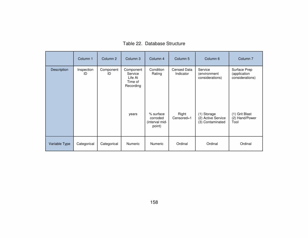
158
Table 22. Database Structure
Column 1 Column 2 Column 3 Column 4 Column 5 Column 6 Column 7
Description Inspection ID
Component ID
Component Service Life At Time of
Recording
years
Condition Rating
% surface corroded
(interval mid-point)
Censed Data Indicator
Right Censored=1
Service (environment considerations) (1) Storage (2) Active Service (3) Contaminated
Surface Prep (application considerations) (1) Grit Blast (2) Hand/Power Tool
Variable Type Categorical Categorical Numeric Numeric Ordinal Ordinal Ordinal

159
APPENDIX B - FIGURES

160
Figure 30. Literature Review Appearance in Publications
0
2
4
6
8
10
1219
92
19
93
19
94
19
95
19
96
19
97
19
98
19
99
20
00
20
01
20
02
20
03
20
04
20
05
20
06
20
07
20
08
20
09
20
10
Qu
an
tity
Year
Appearance in Publications
Optimization CaseStudies
Optimization Methods &Techniques
Source: Sharma et al., "A literature review and future perspectives on maintenance optimization,"

161
Figure 31. Coating System Failure Modes
Source: Martin et al., "Methodologies for predicting the service lives of coating systems," 1994
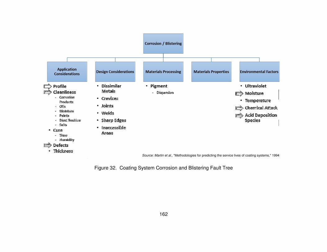
162
Figure 32. Coating System Corrosion and Blistering Fault Tree
Source: Martin et al., "Methodologies for predicting the service lives of coating systems," 1994

163
Figure 33. Coating System & Substrate Cross Section With Faults
Scale: None

164
Figure 34. ASTM D610 Rust Ratings

165
Figure 35. ASTM D714 Blister Ratings

166
Figure 36. Database Structure & Mapping
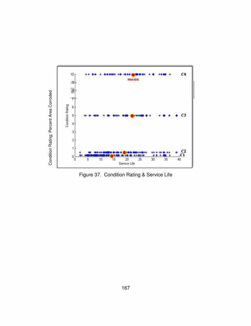
167
Figure 37. Condition Rating & Service Life
Cond
ition R
ating;
Perc
ent
Are
a C
orr
ode
d

168
Figure 38. Time of Failure for Factors

169
VITA
Greg Bosco received a Bachelor of Science in Civil Engineering with a focus on
Structural Engineering from Old Dominion University in 1999. He went on to
receive a Master of Science in Engineering Management from The George
Washington University in 2010. With the University of Tennessee, he continued
graduate level work, studying Reliability and Maintainability Engineering,
specializing in prognostics. He is also a licensed Professional Engineering in the
Commonwealth of Virginia.