Practical Dynamic Programming:An Introduction

Associated programsdpexample.m: deterministicdpexample2.m: stochastic

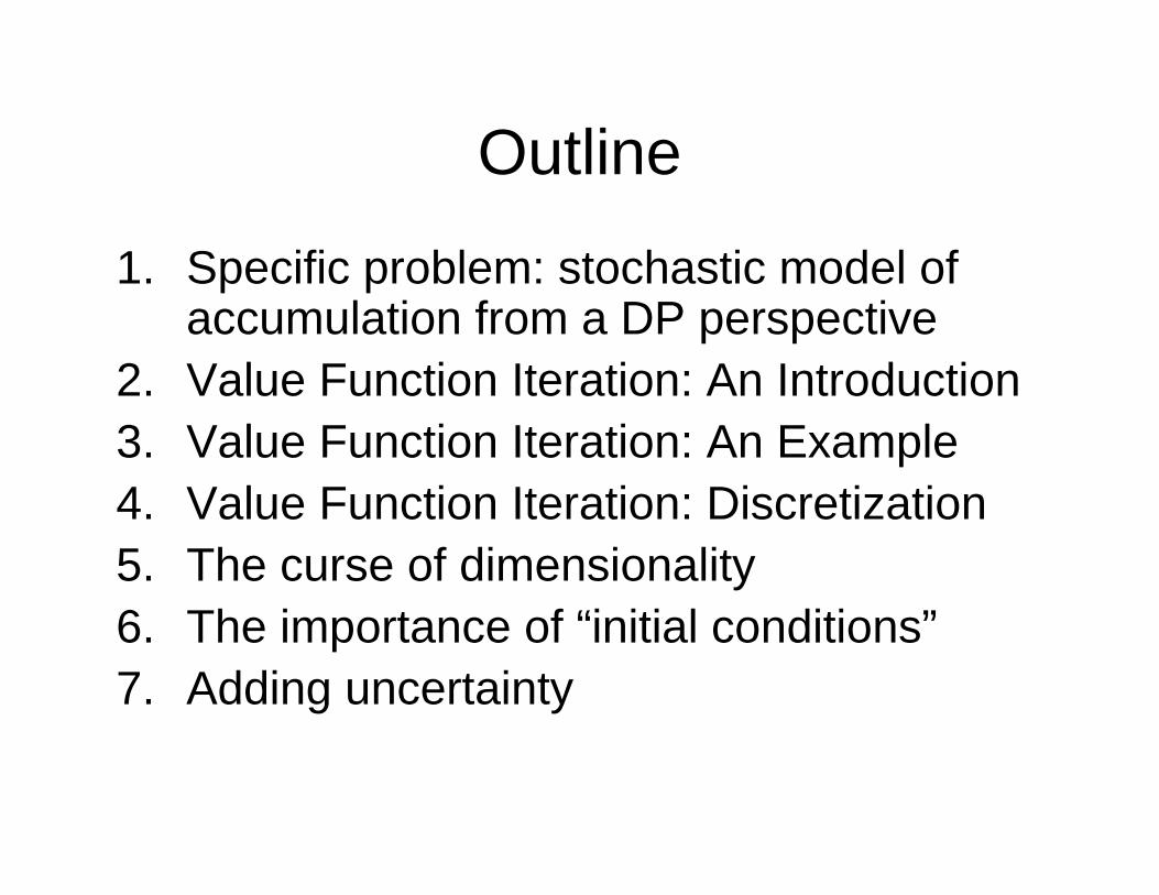
Outline

1. Specific problem: stochastic model of accumulation from a DP perspective

2. Value Function Iteration: An Introduction3. Value Function Iteration: An Example4. Value Function Iteration: Discretization5. The curse of dimensionality 6. The importance of “initial conditions”7. Adding uncertainty

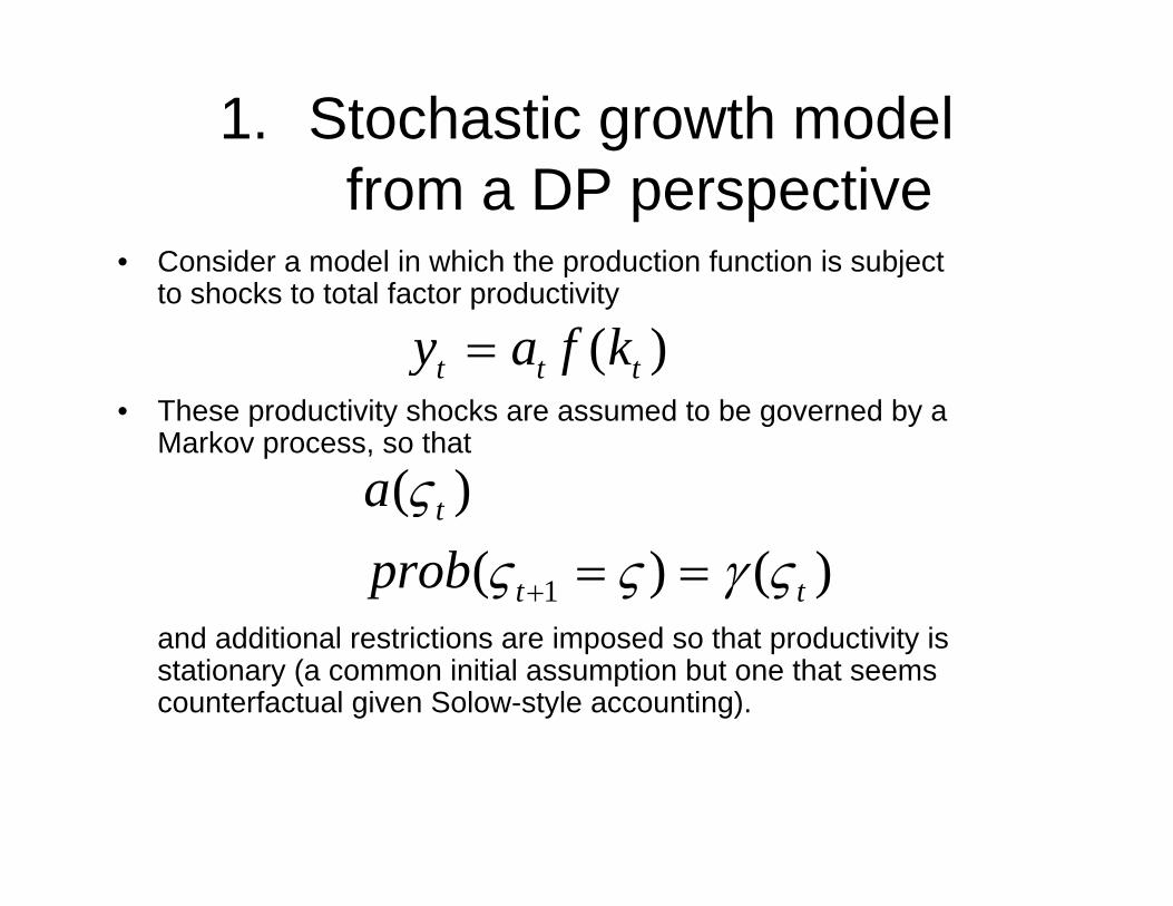
1. Stochastic growth modelfrom a DP perspective

• Consider a model in which the production function is subject to shocks to total factor productivity

• These productivity shocks are assumed to be governed by a Markov process, so that

and additional restrictions are imposed so that productivity is stationary (a common initial assumption but one that seems counterfactual given Solow-style accounting).

( )t t ty a f k=

1

( )( ) ( )

t

t t

aprob

ςς ς γ ς+ = =

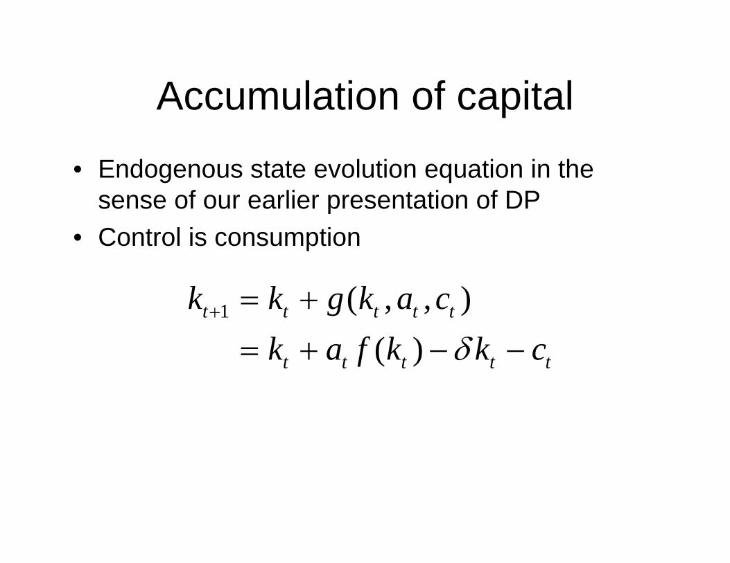
Accumulation of capital

• Endogenous state evolution equation in the sense of our earlier presentation of DP

• Control is consumption

1 ( , , )( )

t t t t t

t t t t t

k k g k a ck a f k k cδ

+ = += + − −

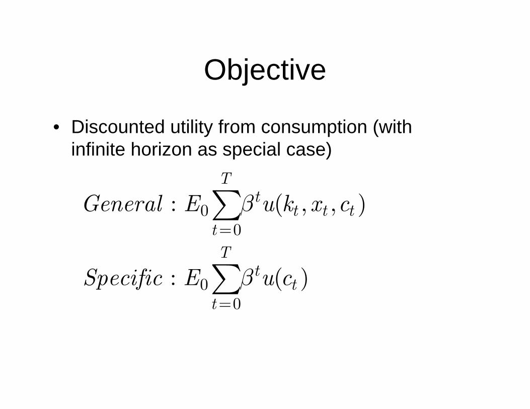
Objective

• Discounted utility from consumption (with infinite horizon as special case)

00

00

: ( , , )

: ( )

Tt

t t ttT

tt

t

General E u k x c

Specific E u c

β

β

=

=

∑

∑

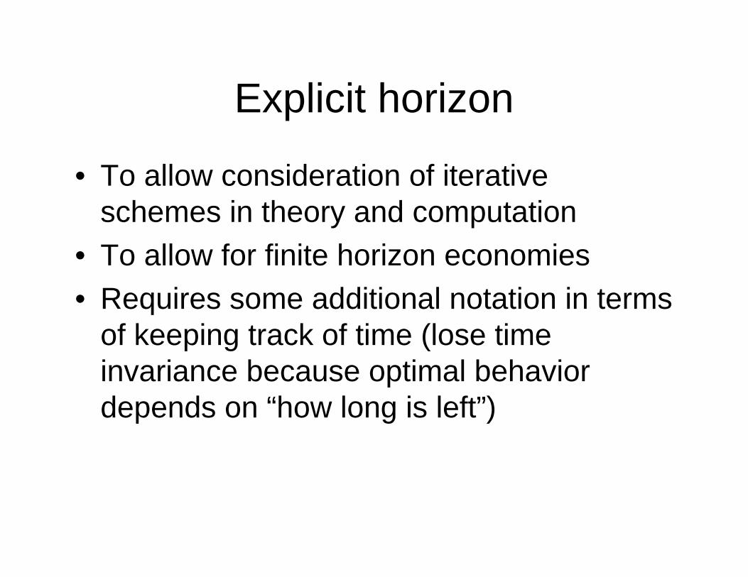
Explicit horizon

• To allow consideration of iterative schemes in theory and computation

• To allow for finite horizon economies• Requires some additional notation in terms

of keeping track of time (lose time invariance because optimal behavior depends on “how long is left”)

2. Value Function Iteration

• We now describe an iterative method of determining value functions for a series of problems with increasing horizon

• This approach is a practical one introduced by Bellman in his original work on dynamic programming.

Review of Bellman’s core ideas• Focused on finding “policy function” and “value

function” both of which depend on states (endogenous and exogenous states).de

• Subdivided complicated intertemporal problems into many “two period” problems, in which the trade-off is between the present “now” and “later”.

• Working principal was to find the optimal control and state “now”, taking as given that latter behavior would itself be optimal.

The Principle of Optimality

• “An optimal policy has the property that, whatever the state and optimal first decision may be, the remaining decisions constitute an optimal policy with respect to the state originating from the first decisions”—Bellman (1957, pg. 83)

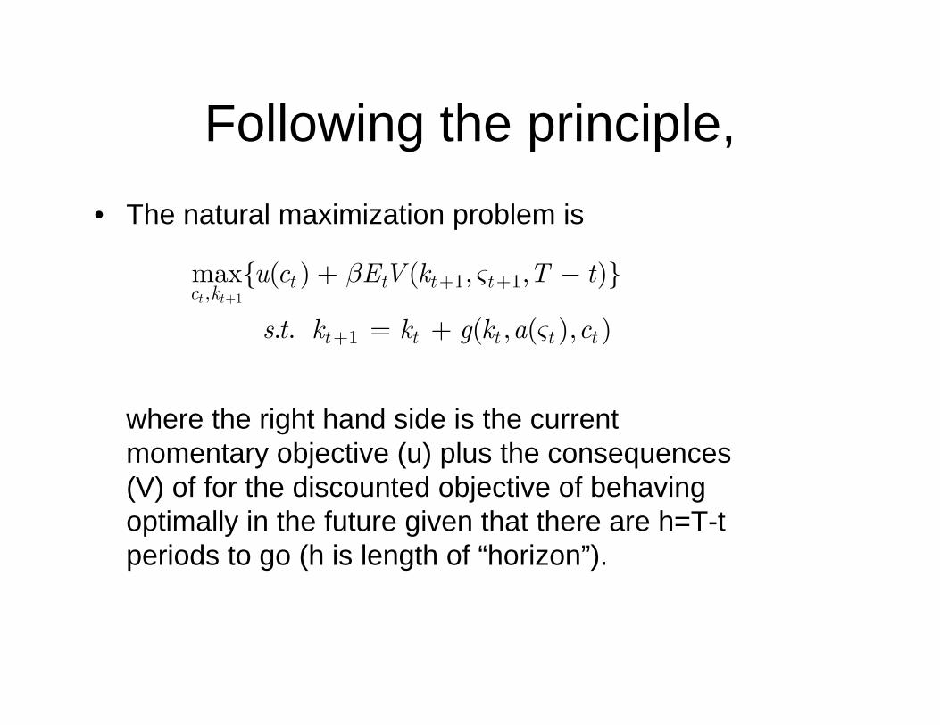
Following the principle, • The natural maximization problem is

where the right hand side is the current momentary objective (u) plus the consequences (V) of for the discounted objective of behaving optimally in the future given that there are h=T-t periods to go (h is length of “horizon”).

11 1,

1

max{ ( ) ( , , )}

. . ( , ( ), )t t

t t t tc k

t t t t t

u c EV k T t

s t k k g k a c

β ς

ς+

+ +

+

+ −

= +

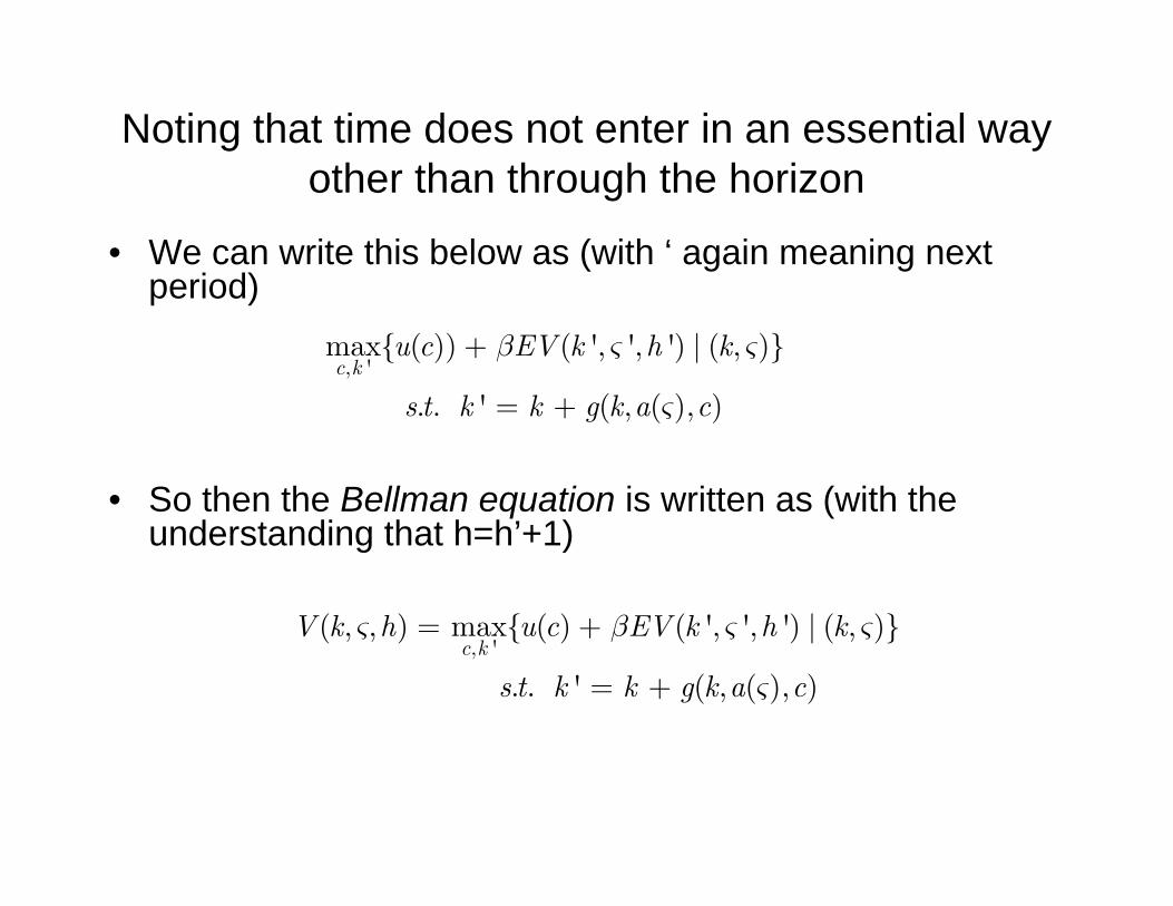
Noting that time does not enter in an essential way other than through the horizon

• We can write this below as (with ‘ again meaning next period)

• So then the Bellman equation is written as (with the understanding that h=h’+1)

, 'max{ ( )) ( ', ', ') | ( , )}

. . ' ( , ( ), )c ku c EV k h k

s t k k g k a c

β ς ς

ς

+

= +

, '( , , ) max{ ( ) ( ', ', ') | ( , )}

. . ' ( , ( ), )c k

V k h u c EV k h k

s t k k g k a c

ς β ς ς

ς

= +

= +

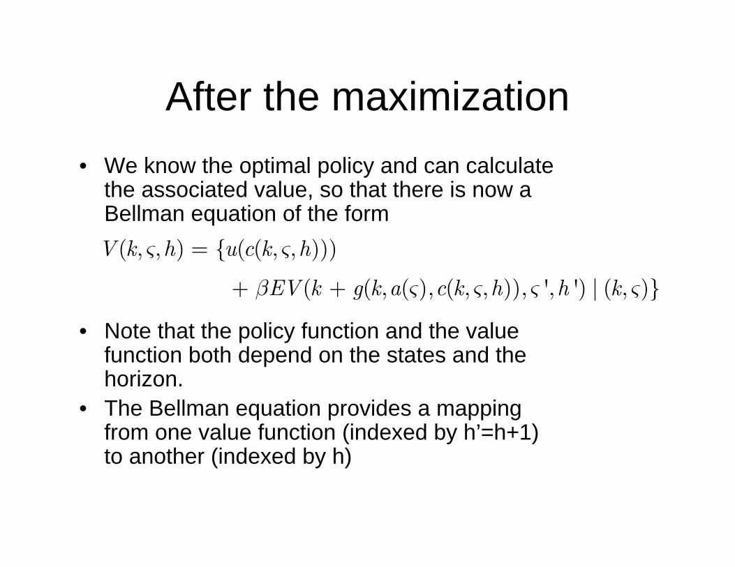
After the maximization• We know the optimal policy and can calculate

the associated value, so that there is now a Bellman equation of the form

• Note that the policy function and the value function both depend on the states and the horizon.

• The Bellman equation provides a mapping from one value function (indexed by h’=h+1) to another (indexed by h)

( , , ) { ( ( , , )))

( ( , ( ), ( , , )), ', ') | ( , )}

V k h u c k h

EV k g k a c k h h k

ς ς

β ς ς ς ς

=

+ +

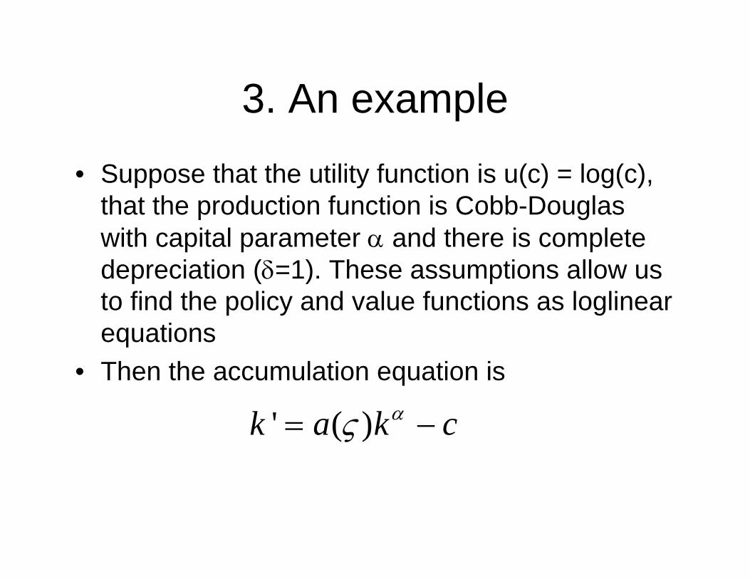
3. An example

• Suppose that the utility function is u(c) = log(c), that the production function is Cobb-Douglas with capital parameter α and there is complete depreciation (δ=1). These assumptions allow us to find the policy and value functions as loglinearequations

• Then the accumulation equation is

' ( )k a k cας= −

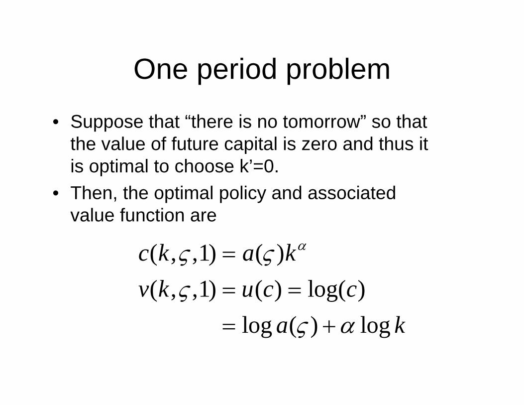
One period problem

• Suppose that “there is no tomorrow” so that the value of future capital is zero and thus it is optimal to choose k’=0.

• Then, the optimal policy and associated value function are

( , ,1) ( )( , ,1) ( ) log( )

log ( ) log

c k a kv k u c c

a k

ας ςς

ς α

== == +

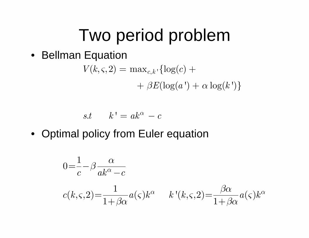
Two period problem• Bellman Equation

• Optimal policy from Euler equation

, '( , , 2) max {log( )

(log( ') log( ')}

. '

c kV k c

E a k

s t k ak cα

ς

β α

= +

+ +

= −

10

1( , ,2) ( ) '( , ,2) ( )

1 1

c ak c

c k a k k k a k

α

α α

αβ

βας ς ς ςβα βα

= −−

= =+ +

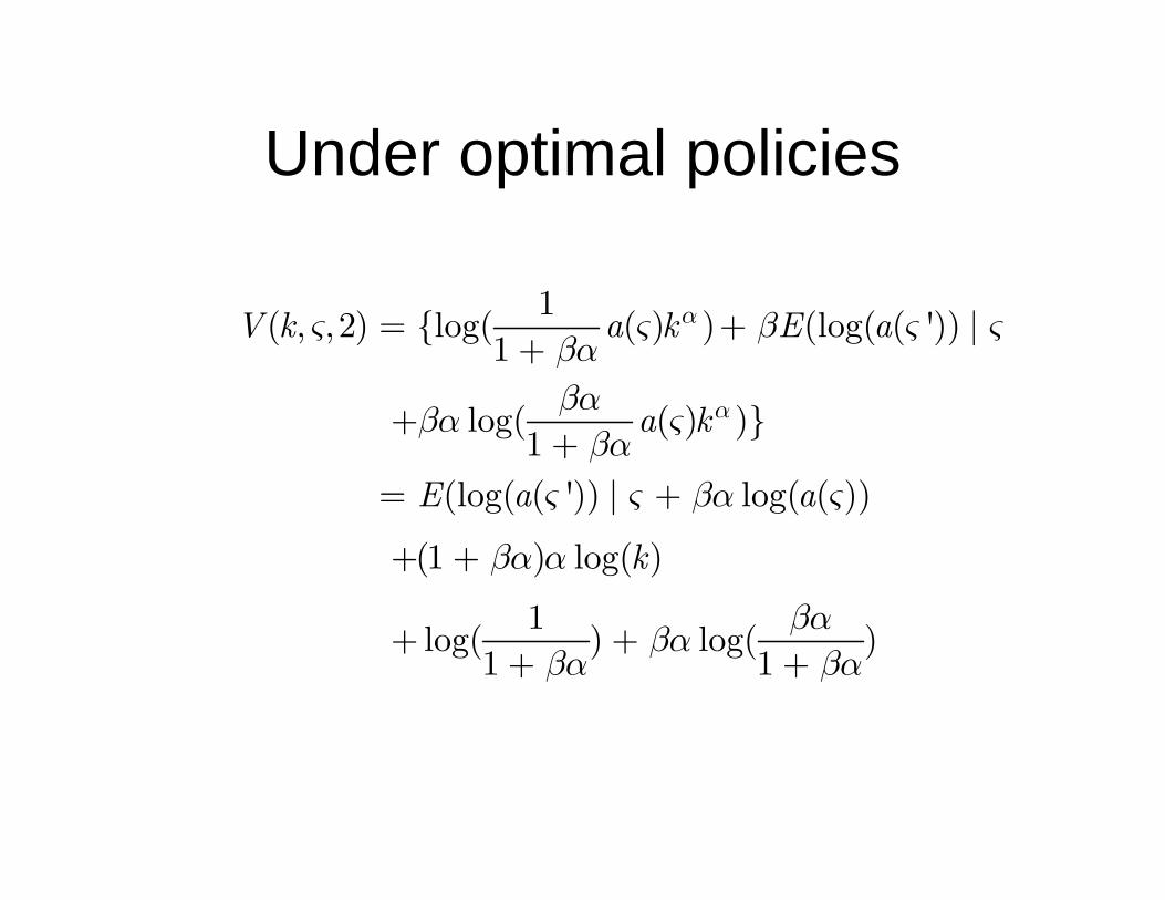
Under optimal policies

1( , , 2) {log( ( ) ) (log( ( ')) |1

log( ( ) )}1

(log( ( ')) | log( ( ))

(1 ) log( )

1log( ) log( )1 1

V k a k E a

a k

E a a

k

α

α

ς ς β ς ςβαβαβα ςβα

ς ς βα ς

βα α

βαβαβα βα

= ++

++

= +

+ +

+ ++ +

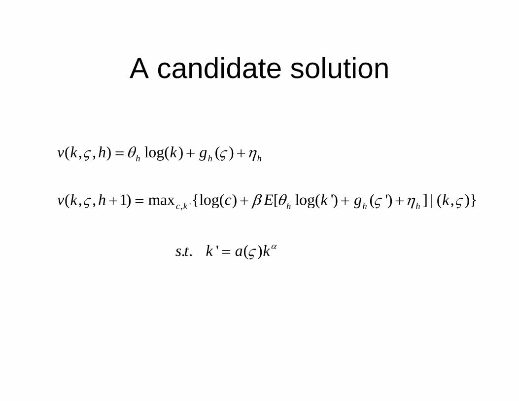
A candidate solution

, '

( , , ) log( ) ( )

( , , 1) max {log( ) [ log( ') ( ') ] | ( , )}

. . ' ( )

h h h

c k h h h

v k h k g

v k h c E k g k

s t k a kα

ς θ ς η

ς β θ ς η ς

ς

= + +

+ = + + +

=

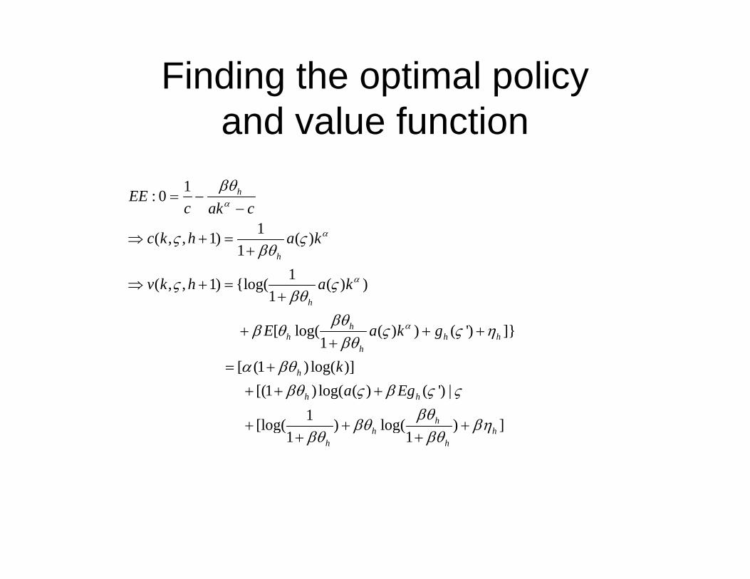
Finding the optimal policy and value function

1: 0

1( , , 1) ( )1

1( , , 1) {log( ( ) )1

[ log( ( ) ) ( ') ]}1

[ (1 ) log( )][(1 ) log( ( ) ( ') |

1[log( ) log( ) ]1 1

h

h

h

hh h h

h

h

h h

hh h

h h

EEc ak c

c k h a k

v k h a k

E a k g

ka Eg

α

α

α

α

βθ

ς ςβθ

ς ςβθ

βθβ θ ς ς η

βθα βθ

βθ ς β ς ςβθ

βθ βηβθ βθ

= −−

⇒ + =+

⇒ + =+

+ + ++

= ++ + +

+ + ++ +

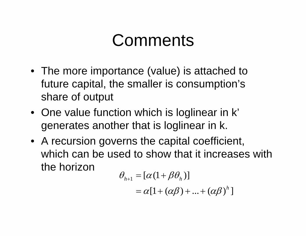
Comments

• The more importance (value) is attached to future capital, the smaller is consumption’s share of output

• One value function which is loglinear in k’generates another that is loglinear in k.

• A recursion governs the capital coefficient, which can be used to show that it increases with the horizon

1 [ (1 )]

[1 ( ) ... ( ) ]h h

h

θ α βθ

α αβ αβ+ = +

= + + +

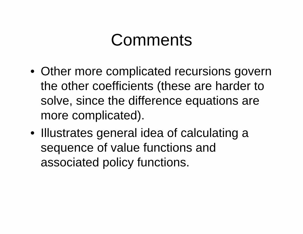
Comments

• Other more complicated recursions govern the other coefficients (these are harder to solve, since the difference equations are more complicated).

• Illustrates general idea of calculating a sequence of value functions and associated policy functions.

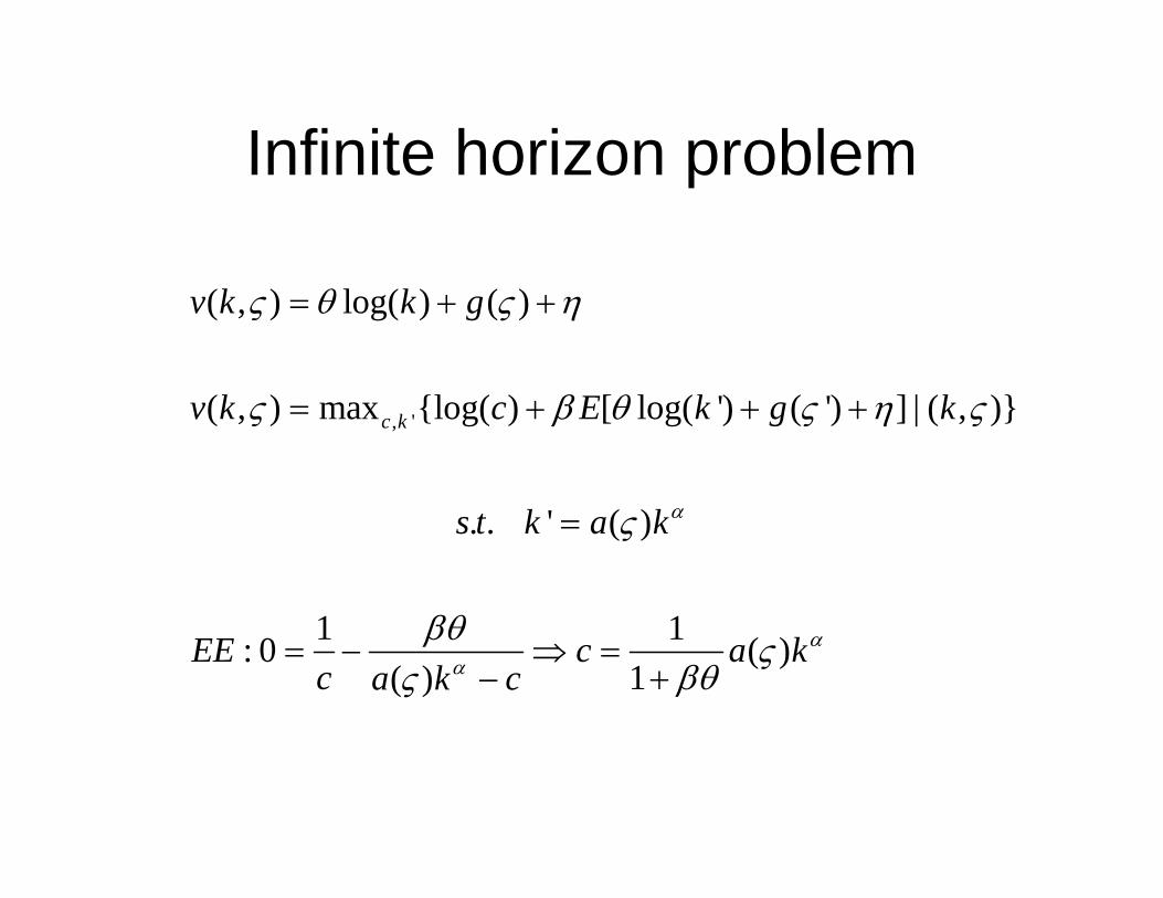
Infinite horizon problem

, '

( , ) log( ) ( )

( , ) max {log( ) [ log( ') ( ') ] | ( , )}

. . ' ( )

1 1: 0 ( )1( )

c k

v k k g

v k c E k g k

s t k a k

EE c a kc a k c

α

αα

ς θ ς η

ς β θ ς η ς

ς

βθ ςβθς

= + +

= + + +

=

= − ⇒ =+−

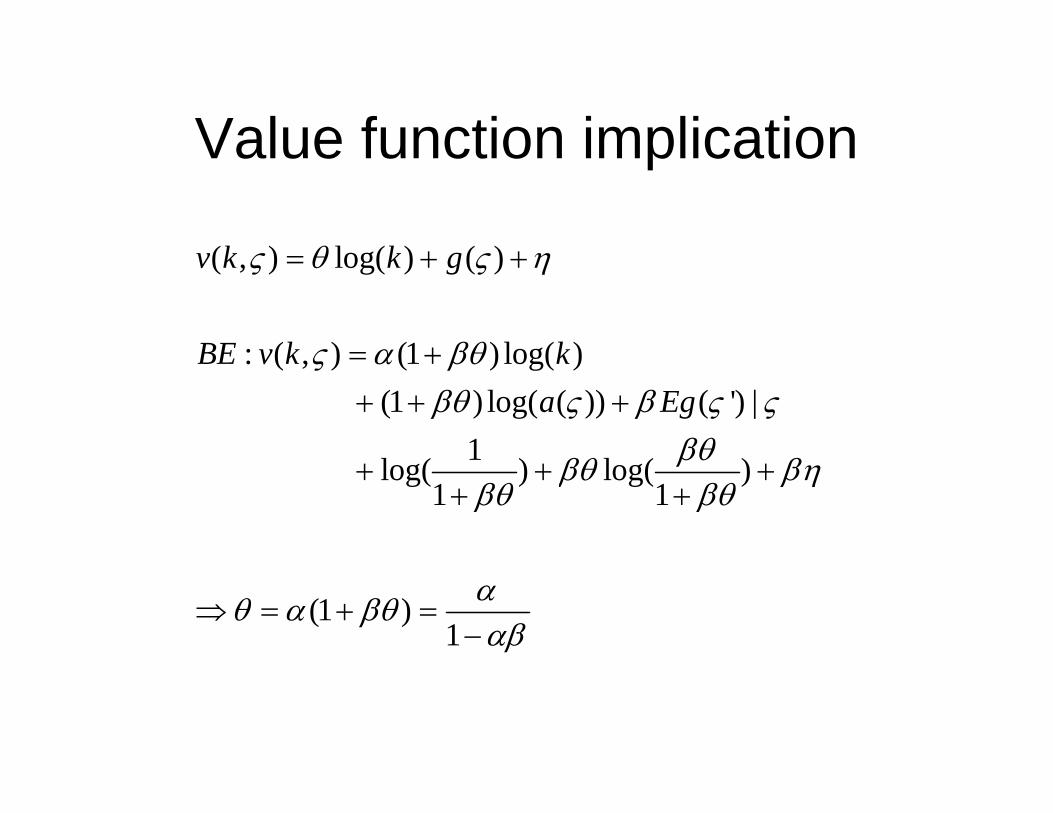
Value function implication

( , ) log( ) ( )

: ( , ) (1 ) log( )(1 ) log( ( )) ( ') |

1log( ) log( )1 1

(1 )1

v k k g

BE v k ka Eg

ς θ ς η

ς α βθβθ ς β ς ς

βθβθ βηβθ βθ

αθ α βθαβ

= + +

= ++ + +

+ + ++ +

⇒ = + =−

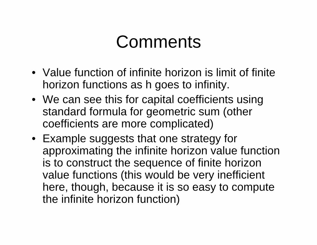
Comments• Value function of infinite horizon is limit of finite

horizon functions as h goes to infinity. • We can see this for capital coefficients using

standard formula for geometric sum (other coefficients are more complicated)

• Example suggests that one strategy for approximating the infinite horizon value function is to construct the sequence of finite horizon value functions (this would be very inefficient here, though, because it is so easy to compute the infinite horizon function)

Comments (contd)

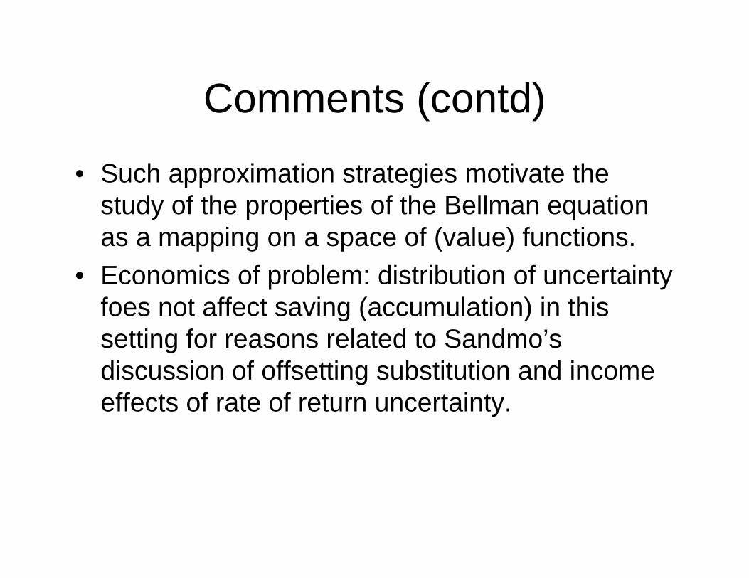
• Such approximation strategies motivate the study of the properties of the Bellman equation as a mapping on a space of (value) functions.

• Economics of problem: distribution of uncertainty foes not affect saving (accumulation) in this setting for reasons related to Sandmo’sdiscussion of offsetting substitution and income effects of rate of return uncertainty.

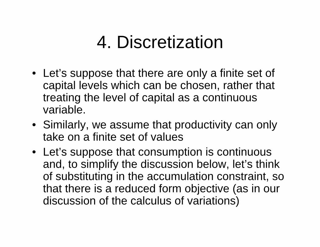
4. Discretization• Let’s suppose that there are only a finite set of

capital levels which can be chosen, rather that treating the level of capital as a continuous variable.

• Similarly, we assume that productivity can only take on a finite set of values

• Let’s suppose that consumption is continuous and, to simplify the discussion below, let’s think of substituting in the accumulation constraint, so that there is a reduced form objective (as in our discussion of the calculus of variations)

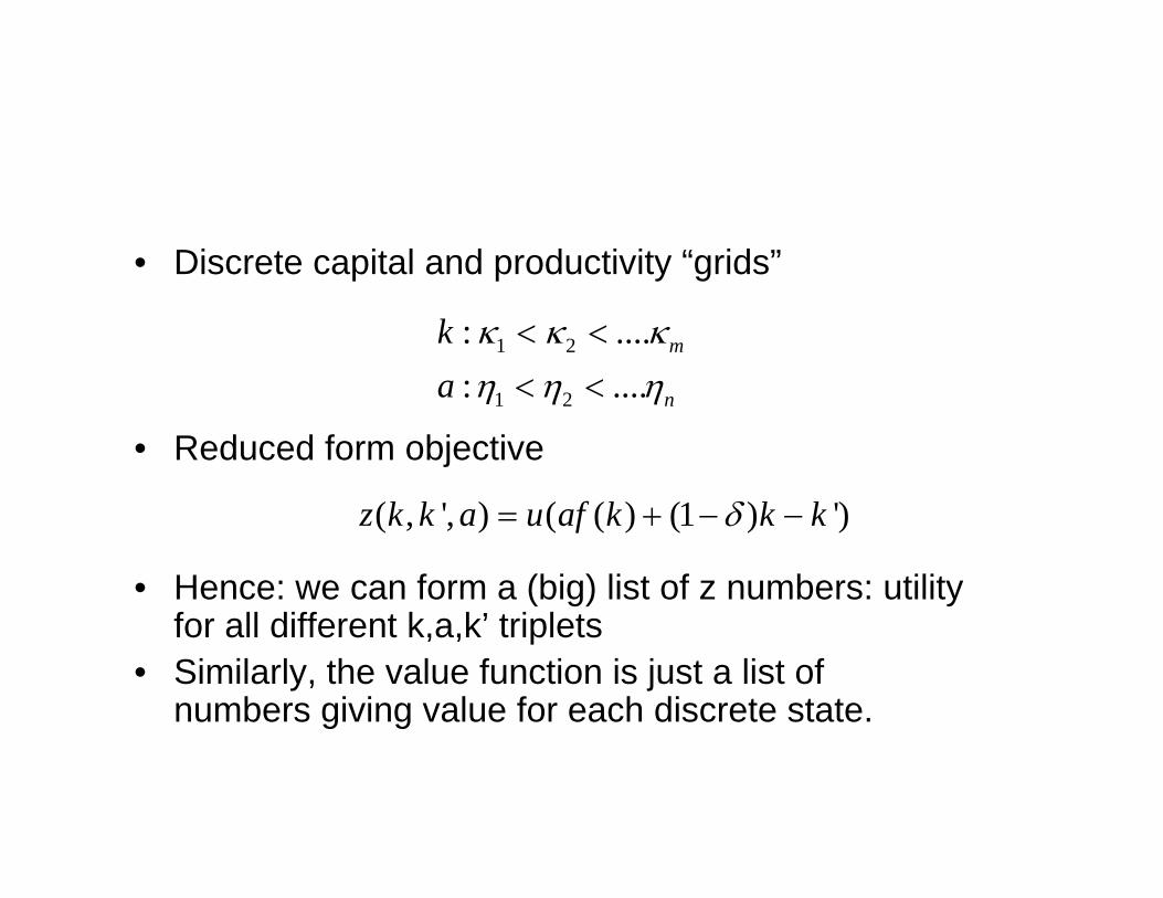
• Discrete capital and productivity “grids”

• Reduced form objective

• Hence: we can form a (big) list of z numbers: utility for all different k,a,k’ triplets

• Similarly, the value function is just a list of numbers giving value for each discrete state.

1 2

1 2

: ....: ....

m

n

ka

κ κ κη η η

< <

< <

( , ', ) ( ( ) (1 ) ')z k k a u af k k kδ= + − −

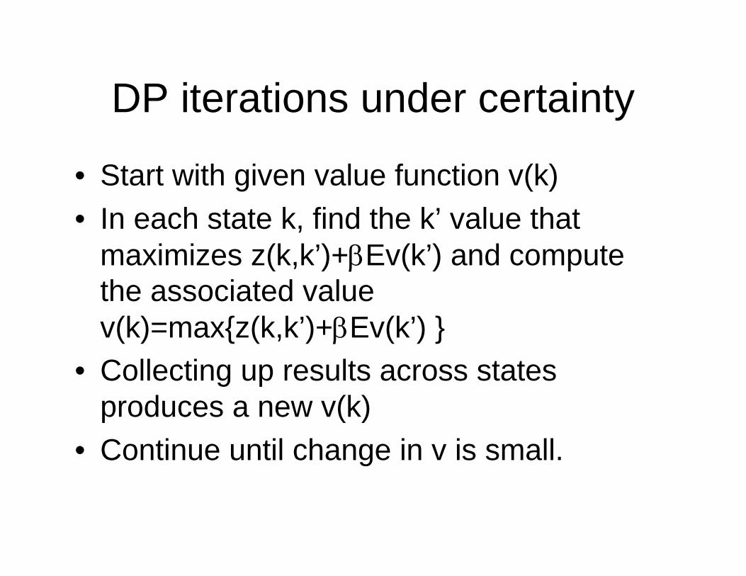
DP iterations under certainty

• Start with given value function v(k)• In each state k, find the k’ value that

maximizes z(k,k’)+βEv(k’) and compute the associated value v(k)=max{z(k,k’)+βEv(k’) }

• Collecting up results across states produces a new v(k)

• Continue until change in v is small.

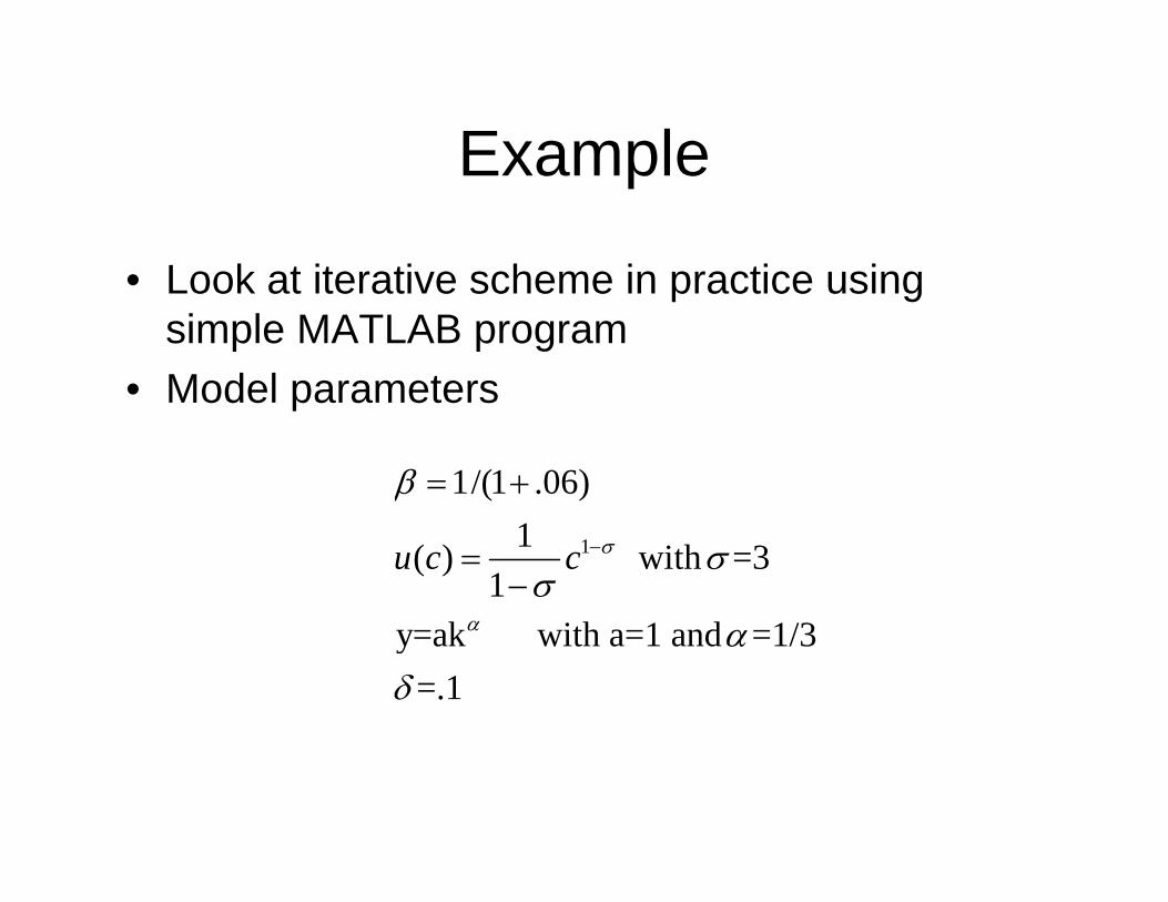
Example

• Look at iterative scheme in practice using simple MATLAB program

• Model parameters

1

1/(1 .06)1( ) with =3

1y=ak with a=1 and =1/3

=.1

u c c σ

α

β

σσ

αδ

−

= +

=−

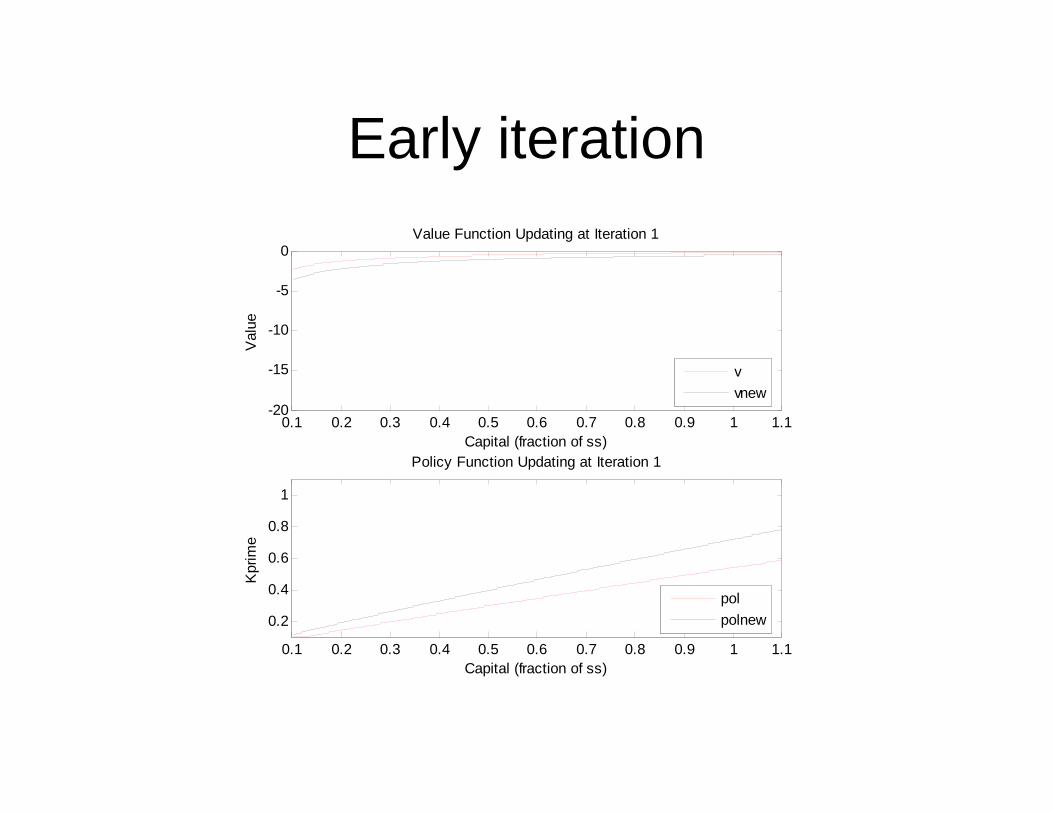
Early iteration

0.1 0.2 0.3 0.4 0.5 0.6 0.7 0.8 0.9 1 1.1-20

-15

-10

-5

0Value Function Updating at Iteration 1

Capital (fraction of ss)

Val

ue

0.1 0.2 0.3 0.4 0.5 0.6 0.7 0.8 0.9 1 1.1

0.2

0.4

0.6

0.8

1

Policy Function Updating at Iteration 1

Capital (fraction of ss)

Kpr

ime

vvnew

polpolnew

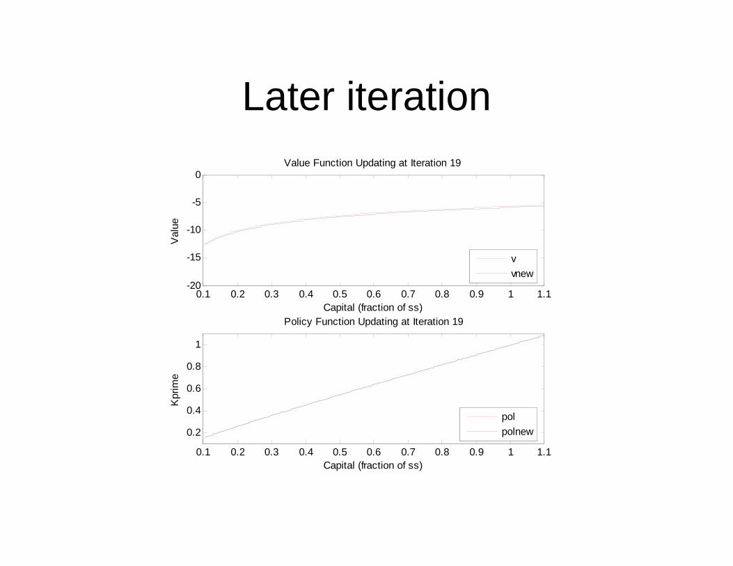
Later iteration

0.1 0.2 0.3 0.4 0.5 0.6 0.7 0.8 0.9 1 1.1-20

-15

-10

-5

0Value Function Updating at Iteration 19

Capital (fraction of ss)

Val

ue

0.1 0.2 0.3 0.4 0.5 0.6 0.7 0.8 0.9 1 1.1

0.2

0.4

0.6

0.8

1

Policy Function Updating at Iteration 19

Capital (fraction of ss)

Kpr

ime

vvnew

polpolnew

Lessons: Specific and General• Value function to converge more slowly than policy

function: welfare is more sensitive to horizon than behavior.– Has motivated work on “policy iteration” where one starts with an

initial policy (say, a linear approximation policy); evaluates the value function; finds a new policy that maximizes z(k,k’)+βEv(k’) and then iterates until the policy converged.

– Has motivated development of “acceleration algorithms”Example: evaluate value under some feasible policy (say constant saving rate policy) and then use this as the starting point for value iteration

• Policy function looks pretty linear.– Has comforted some in use of linear approximation methods– Has motivated others to look for “peicewise linear” policy

functions.

5. The Curse of dimensionality• We have studied a model with one state which can taken on N

different values. • Our “brute force” optimization approach involves calculating z(k,k’)

at each k for each possible k’ and then picking the largest one. Hence, we have to compute z(k,k’) a total of N*N times.

• If we have a “good” method of finding the optimal policy in at each point k, such as using properties of the objective, then the problem might only involve NM computations (with M<N being the smaller number of steps in the maximization step).

• Suppose that there were two states, each of which can take on N different values. We would have to find an optimal state evolution at each of N*N points and a blind search would require evaluating z at N*N points – all of the possible actions -- for each at each state. A more sophisticated search would require (N*N*M), as we would be doing M computations at each of N*N points in a state “grid”.

Curse• Even if computation is maximially efficient (M=1,

so that one does only one evaluation of Z at each point in a state grid), one can see that this state grid gets “large” very fast: if there are j states then there are Nj points in the grid: with 100 points for each state and 4 state variables, one is looking at a grid of 108 of points.

• Discretization methods are not feasible for complicated models with many states. Has motivated study of many other computational procedures for dynamic programming.

6. The importanceof initial conditions

• We started the example dynamic programs with a future v=0 and with v(k,a,0)=u(af(k)+(1-δ)k) .

• Theorems in the literature on dynamic programming guarantee the convergence of value function iteration – under specified conditions on u,f,a – from any initial condition. In this sense, the initial condition is irrelevant. Such theorems will be developed in Miao’s “Economic Dynamics” course in the spring.

• However, the theorems indicate that for a large number of iterations, results from any two starting points are (i) arbitrarily close to each other and (ii) arbitrarily close to the solution for the infinite horizon case.

• In a practical sense, initial conditions can be critical. Imagine that, by accident or design, one started off with exactly the correct value function for the infinite horizon case, but you did not know the policy function. In this situation, there would only be one iteration, because the infinite horizon Bellman equation means that the “new” v will be equal to the “old” v.

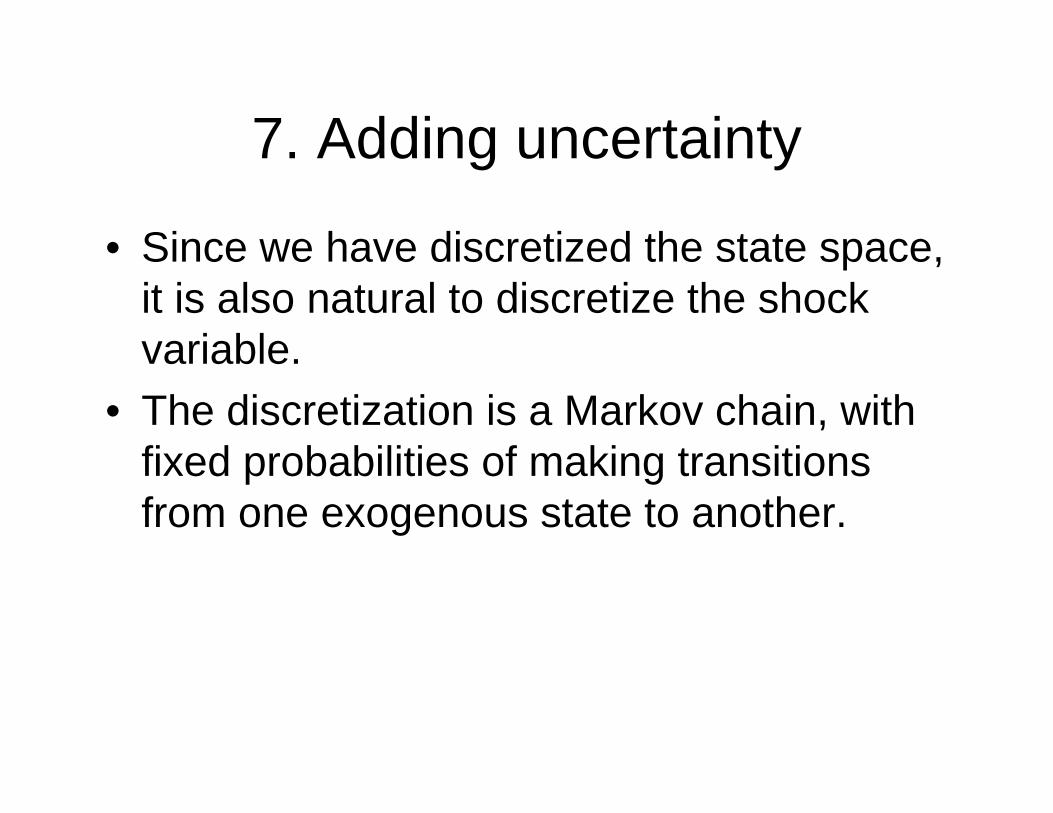
7. Adding uncertainty

• Since we have discretized the state space, it is also natural to discretize the shock variable.

• The discretization is a Markov chain, with fixed probabilities of making transitions from one exogenous state to another.

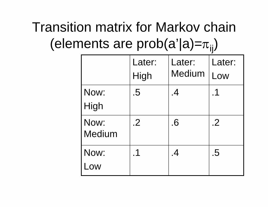
Transition matrix for Markov chain(elements are prob(a’|a)=πij)

.5.4 .1Now: Low

.2.6.2Now: Medium

.1.4.5Now:High

Later:Low

Later: Medium

Later:High

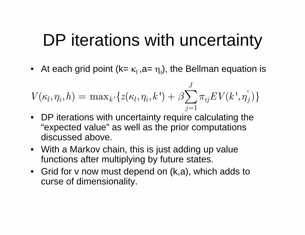
DP iterations with uncertainty• At each grid point (k= κl ,a= ηi), the Bellman equation is

• DP iterations with uncertainty require calculating the “expected value” as well as the prior computations discussed above.

• With a Markov chain, this is just adding up value functions after multiplying by future states.

• Grid for v now must depend on (k,a), which adds to curse of dimensionality.

''

1( , , ) max { ( , , ') ( ', )}

J

l i k l i ij jj

V h z k EV kκ η κ η β π η=

= + ∑

Stochastic dynamic program

• Three value functions in graph: each of three values of “a”

• Three policy functions in graph: each of three values of “a”.

• No longer see “improvements” for all three: just the middle “a” function to avoid graphical clutter (it is the dashed line).

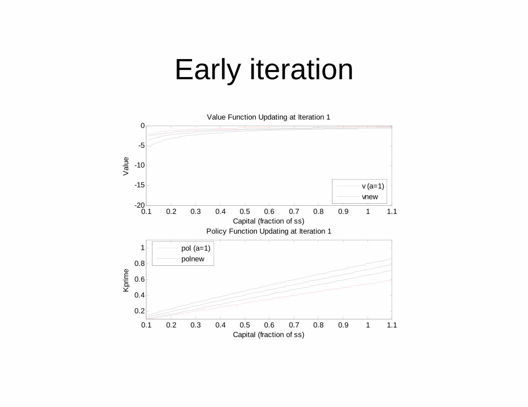
Early iteration

0.1 0.2 0.3 0.4 0.5 0.6 0.7 0.8 0.9 1 1.1-20

-15

-10

-5

0Value Function Updating at Iteration 1

Capital (fraction of ss)

Val

ue

0.1 0.2 0.3 0.4 0.5 0.6 0.7 0.8 0.9 1 1.1

0.2

0.4

0.6

0.8

1

Policy Function Updating at Iteration 1

Capital (fraction of ss)

Kpr

ime

v (a=1)vnew

pol (a=1)polnew

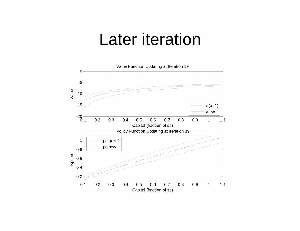
Later iteration

0.1 0.2 0.3 0.4 0.5 0.6 0.7 0.8 0.9 1 1.1-20

-15

-10

-5

0Value Function Updating at Iteration 19

Capital (fraction of ss)

Val

ue

0.1 0.2 0.3 0.4 0.5 0.6 0.7 0.8 0.9 1 1.1

0.2

0.4

0.6

0.8

1

Policy Function Updating at Iteration 19

Capital (fraction of ss)

Kpr

ime

v (a=1)vnew

pol (a=1)polnew