Practical algorithms for constructing HKZ and Minkowski

reduced bases

Wen Zhang, Sanzheng Qiao, and Yimin Wei

April 20, 2011

Abstract

In this paper, three practical lattice basis reduction algorithms are presented. The firstalgorithm constructs a Hermite, Korkine and Zolotareff (HKZ) reduced lattice basis, inwhich a unimodular transformation is used for basis expansion. Our complexity analysisshows that our algorithm is significantly more efficient than the existing HKZ reductionalgorithms. The second algorithm computes a Minkowski reduced lattice basis. It is thefirst practical algorithm for Minkowski reduced bases for lattices of arbitrary dimensions.The third algorithm is an improvement of the second algorithm by drastically reducing thenumber of lattice points being searched. Since the original LLL algorithm is no longerapplicable to the third algorithm, we propose a notion of quasi-LLL reduction to acceleratethe computation.

Keywords Lattice, LLL reduced basis, HKZ reduced basis, Minkowski reduced basis, unimod-ular transformation.

1 Introduction

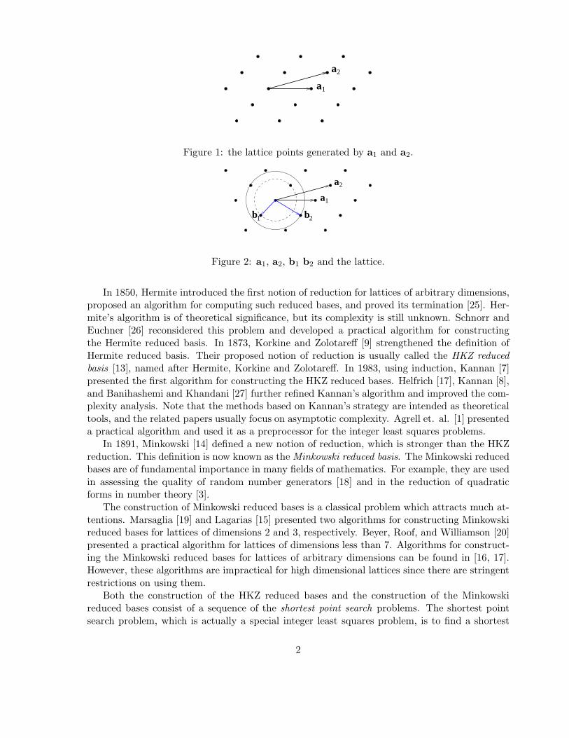
A lattice is a set of discrete points representing integer linear combinations of linearly indepen-dent vectors. The set of linearly independent vectors generating a lattice is called a basis forthe lattice. A lattice basis is usually not unique, but all the bases have the same number ofelements, called the dimension of the lattice. If the dimension of a lattice is larger than 1, thereare infinitely many bases. For example, Figure 1 depicts the lattice generated by a1 = [2.0, 0]T

and a2 = [2.7, 0.7]T . This lattice has dimension 2, and for any integer c, a1 and a2 + c · a1 forma basis for this lattice.

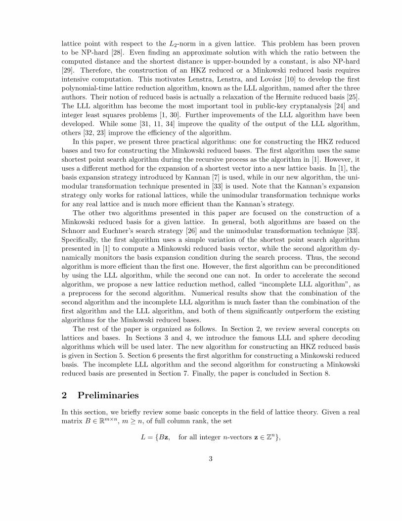
Since a lattice can have more than one basis, it is desirable to find one that is nearlyorthogonal. It is reasonable to expect that the shorter the basis vectors are, the nearer they areto orthogonal. For example, b1 = [−0.7,−0.7]T and b2 = [1.3,−0.7]T form another basis forthe lattice Figure 1. Figure 2 shows that the basis vectors b1 and b2 are shorter than a1 anda2 with respect to the L2-norm, and they are nearer to orthogonal than a1 and a2.

A lattice basis consisting of relatively short vectors is called reduced. An ideally reducedbasis consists of shortest possible vectors. The problem of finding good reduced bases is knownas lattice reduction, which plays an important role in many fields of mathematics and computerscience [3, 4, 13, 18, 21], particularly in communications [1, 23] and cryptology [6, 22]. Thereare vavious definitions of reduced bases. They differ in the degree of reduction.

1

2

a1

a

Figure 1: the lattice points generated by a1 and a2.

2

a1

a2

b1 b

Figure 2: a1, a2, b1 b2 and the lattice.

In 1850, Hermite introduced the first notion of reduction for lattices of arbitrary dimensions,proposed an algorithm for computing such reduced bases, and proved its termination [25]. Her-mite’s algorithm is of theoretical significance, but its complexity is still unknown. Schnorr andEuchner [26] reconsidered this problem and developed a practical algorithm for constructingthe Hermite reduced basis. In 1873, Korkine and Zolotareff [9] strengthened the definition ofHermite reduced basis. Their proposed notion of reduction is usually called the HKZ reducedbasis [13], named after Hermite, Korkine and Zolotareff. In 1983, using induction, Kannan [7]presented the first algorithm for constructing the HKZ reduced bases. Helfrich [17], Kannan [8],and Banihashemi and Khandani [27] further refined Kannan’s algorithm and improved the com-plexity analysis. Note that the methods based on Kannan’s strategy are intended as theoreticaltools, and the related papers usually focus on asymptotic complexity. Agrell et. al. [1] presenteda practical algorithm and used it as a preprocessor for the integer least squares problems.

In 1891, Minkowski [14] defined a new notion of reduction, which is stronger than the HKZreduction. This definition is now known as the Minkowski reduced basis. The Minkowski reducedbases are of fundamental importance in many fields of mathematics. For example, they are usedin assessing the quality of random number generators [18] and in the reduction of quadraticforms in number theory [3].

The construction of Minkowski reduced bases is a classical problem which attracts much at-tentions. Marsaglia [19] and Lagarias [15] presented two algorithms for constructing Minkowskireduced bases for lattices of dimensions 2 and 3, respectively. Beyer, Roof, and Williamson [20]presented a practical algorithm for lattices of dimensions less than 7. Algorithms for construct-ing the Minkowski reduced bases for lattices of arbitrary dimensions can be found in [16, 17].However, these algorithms are impractical for high dimensional lattices since there are stringentrestrictions on using them.

Both the construction of the HKZ reduced bases and the construction of the Minkowskireduced bases consist of a sequence of the shortest point search problems. The shortest pointsearch problem, which is actually a special integer least squares problem, is to find a shortest

2

lattice point with respect to the L2-norm in a given lattice. This problem has been provento be NP-hard [28]. Even finding an approximate solution with which the ratio between thecomputed distance and the shortest distance is upper-bounded by a constant, is also NP-hard[29]. Therefore, the construction of an HKZ reduced or a Minkowski reduced basis requiresintensive computation. This motivates Lenstra, Lenstra, and Lovasz [10] to develop the firstpolynomial-time lattice reduction algorithm, known as the LLL algorithm, named after the threeauthors. Their notion of reduced basis is actually a relaxation of the Hermite reduced basis [25].The LLL algorithm has become the most important tool in public-key cryptanalysis [24] andinteger least squares problems [1, 30]. Further improvements of the LLL algorithm have beendeveloped. While some [31, 11, 34] improve the quality of the output of the LLL algorithm,others [32, 23] improve the efficiency of the algorithm.

In this paper, we present three practical algorithms: one for constructing the HKZ reducedbases and two for constructing the Minkowski reduced bases. The first algorithm uses the sameshortest point search algorithm during the recursive process as the algorithm in [1]. However, ituses a different method for the expansion of a shortest vector into a new lattice basis. In [1], thebasis expansion strategy introduced by Kannan [7] is used, while in our new algorithm, the uni-modular transformation technique presented in [33] is used. Note that the Kannan’s expansionstrategy only works for rational lattices, while the unimodular transformation technique worksfor any real lattice and is much more efficient than the Kannan’s strategy.

The other two algorithms presented in this paper are focused on the construction of aMinkowski reduced basis for a given lattice. In general, both algorithms are based on theSchnorr and Euchner’s search strategy [26] and the unimodular transformation technique [33].Specifically, the first algorithm uses a simple variation of the shortest point search algorithmpresented in [1] to compute a Minkowski reduced basis vector, while the second algorithm dy-namically monitors the basis expansion condition during the search process. Thus, the secondalgorithm is more efficient than the first one. However, the first algorithm can be preconditionedby using the LLL algorithm, while the second one can not. In order to accelerate the secondalgorithm, we propose a new lattice reduction method, called “incomplete LLL algorithm”, asa preprocess for the second algorithm. Numerical results show that the combination of thesecond algorithm and the incomplete LLL algorithm is much faster than the combination of thefirst algorithm and the LLL algorithm, and both of them significantly outperform the existingalgorithms for the Minkowski reduced bases.

The rest of the paper is organized as follows. In Section 2, we review several concepts onlattices and bases. In Sections 3 and 4, we introduce the famous LLL and sphere decodingalgorithms which will be used later. The new algorithm for constructing an HKZ reduced basisis given in Section 5. Section 6 presents the first algorithm for constructing a Minkowski reducedbasis. The incomplete LLL algorithm and the second algorithm for constructing a Minkowskireduced basis are presented in Section 7. Finally, the paper is concluded in Section 8.

2 Preliminaries

In this section, we briefly review some basic concepts in the field of lattice theory. Given a realmatrix B ∈ Rm×n, m ≥ n, of full column rank, the set

L = {Bz, for all integer n-vectors z ∈ Zn},

3

containing discrete grid points, is called a lattice generated by B. The linearly independentcolumns of B form a basis for L.

A set of lattice points does not uniquely determine a basis, but all the bases have the samenumber n of elements, called the dimension of L. In general, if Z ∈ Rn×n is an integer matrixwhose inverse is also an integer matrix, then both B and BZ generate the same lattice. Aninteger matrix M ∈ Rn×n is called unimodular if det(M) = ±1, where det(M) denotes thedeterminant of M . It is obvious that an integer nonsingular matrix Z is unimodular if and onlyif its inverse is also integer. Thus two different bases of a lattice are related with each other bya unimodular matrix.

The determinant of a lattice is defined by

det(L) =√

det(BTB),

where B is a generating matrix of the lattice L. From the definition of unimodular, det(BTB) =det((BZ)TBZ), for any unimodular Z. Hence the determinant of a lattice is independent ofthe choice of basis. Actually, the determinant of a lattice can be viewed as the volume of theparallelepiped spanned by a basis for the lattice.

Since a lattice can have many bases, it is desirable to find one that is nearly orthogonal. Theproblem for finding good reduced bases is known as lattice reduction. In terms of matrix, thegoal of lattice reduction is to find a unimodular Z so that the columns of BZ form a reducedbasis.

There are various definitions of a reduced basis, and most of them are based on the orthogonaldecomposition of the lattice generating matrix that can be achieved by the following procedure.

Procedure 1 (Gram-Schmidt Orthogonalization) Given a matrix B = [b1, · · · ,bn] ∈Rm×n, this procedure produces matrices Q∗ and U such that B = Q∗U , where Q∗ ∈ Rm×n

has orthogonal columns and U ∈ Rn×n is upper triangular with a unit diagonal.

1. U ← n× n identity matrix In.2. q∗

1 ← b1.3. for j = 2 : n4. for i = 1 : j − 1

5. U(i, j)←(bj ,q∗

i )

‖q∗

i‖2

2

.

6. end

7. q∗j ← bj −

∑j−1i=1 U(i, j)q∗

i .

8. end9. Q∗ ← [q∗

1, · · · ,q∗n].

Note that the above Gram-Schmidt orthogonalization (GSO) procedure is square-root free.So the GSO can be performed in exact arithmetic for integer or rational lattice generatingmatrices, since all the operations are rational arithmetic. Therefore the GSO is widely used inapplications of cryptology, in which the lattice generating matrices usually appear to be integral[24]. However, the generating matrices in the applications of communications are usually real orcomplex [1, 23], and the computations of the GSO are not numerically stable for such matrices[5]. So in such applications, the GSO is usually replaced by a mathematically equivalent but

4

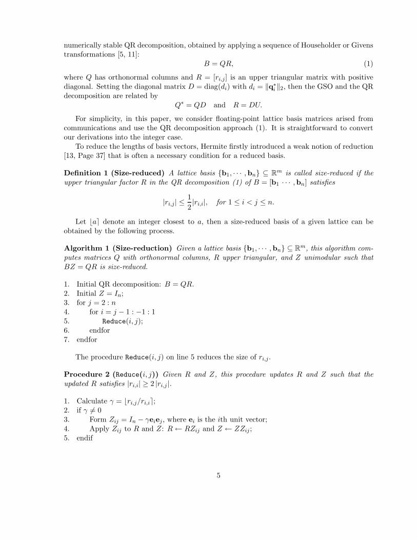
numerically stable QR decomposition, obtained by applying a sequence of Householder or Givenstransformations [5, 11]:

B = QR, (1)

where Q has orthonormal columns and R = [ri,j] is an upper triangular matrix with positivediagonal. Setting the diagonal matrix D = diag(di) with di = ‖q∗

i ‖2, then the GSO and the QRdecomposition are related by

Q∗ = QD and R = DU.

For simplicity, in this paper, we consider floating-point lattice basis matrices arised fromcommunications and use the QR decomposition approach (1). It is straightforward to convertour derivations into the integer case.

To reduce the lengths of basis vectors, Hermite firstly introduced a weak notion of reduction[13, Page 37] that is often a necessary condition for a reduced basis.

Definition 1 (Size-reduced) A lattice basis {b1, · · · ,bn} ⊆ Rm is called size-reduced if theupper triangular factor R in the QR decomposition (1) of B = [b1 · · · ,bn] satisfies

|ri,j| ≤1

2|ri,i|, for 1 ≤ i < j ≤ n.

Let ⌊a⌉ denote an integer closest to a, then a size-reduced basis of a given lattice can beobtained by the following process.

Algorithm 1 (Size-reduction) Given a lattice basis {b1, · · · ,bn} ⊆ Rm, this algorithm com-putes matrices Q with orthonormal columns, R upper triangular, and Z unimodular such thatBZ = QR is size-reduced.

1. Initial QR decomposition: B = QR.2. Initial Z = In;3. for j = 2 : n4. for i = j − 1 : −1 : 15. Reduce(i, j);6. endfor7. endfor

The procedure Reduce(i, j) on line 5 reduces the size of ri,j.

Procedure 2 (Reduce(i, j)) Given R and Z, this procedure updates R and Z such that theupdated R satisfies |ri,i| ≥ 2 |ri,j |.

1. Calculate γ = ⌊ri,j/ri,i⌉;2. if γ 6= 03. Form Zij = In − γeiej , where ei is the ith unit vector;4. Apply Zij to R and Z: R← RZij and Z ← ZZij ;5. endif

5

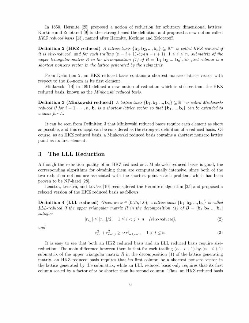
In 1850, Hermite [25] proposed a notion of reduction for arbitrary dimensional lattices.Korkine and Zolotareff [9] further strengthened the definition and proposed a new notion calledHKZ reduced basis [13], named after Hermite, Korkine and Zolotareff.

Definition 2 (HKZ reduced) A lattice basis {b1,b2, ...,bn} ⊆ Rm is called HKZ reduced ifit is size-reduced, and for each trailing (n − i + 1)-by-(n − i + 1), 1 ≤ i ≤ n, submatrix of theupper triangular matrix R in the decomposition (1) of B = [b1 b2 ... bn], its first column is ashortest nonzero vector in the lattice generated by the submatrix.

From Definition 2, an HKZ reduced basis contains a shortest nonzero lattice vector withrespect to the L2-norm as its first element.

Minkowski [14] in 1891 defined a new notion of reduction which is stricter than the HKZreduced basis, known as the Minkowski reduced basis.

Definition 3 (Minkowski reduced) A lattice basis {b1,b2, ...,bn} ⊆ Rm is called Minkowskireduced if for i = 1, · · · , n, bi is a shortest lattice vector so that {b1, ...,bi} can be extended toa basis for L.

It can be seen from Definition 3 that Minkowski reduced bases require each element as shortas possible, and this concept can be considered as the strongest definition of a reduced basis. Ofcourse, as an HKZ reduced basis, a Minkowski reduced basis contains a shortest nonzero latticepoint as its first element.

3 The LLL Reduction

Although the reduction quality of an HKZ reduced or a Minkowski reduced bases is good, thecorresponding algorithms for obtaining them are computationally intensive, since both of thetwo reduction notions are associated with the shortest point search problem, which has beenproven to be NP-hard [28].

Lenstra, Lenstra, and Lovasz [10] reconsidered the Hermite’s algorithm [25] and proposed arelaxed version of the HKZ reduced basis as follows:

Definition 4 (LLL reduced) Given an ω ∈ (0.25, 1.0), a lattice basis {b1,b2, ...,bn} is calledLLL-reduced if the upper triangular matrix R in the decomposition (1) of B = [b1 b2 ... bn]satisfies

|ri,j| ≤ |ri,i|/2, 1 ≤ i < j ≤ n (size-reduced), (2)

andr2i,i + r2

i−1,i ≥ ω r2i−1,i−1, 1 < i ≤ n. (3)

It is easy to see that both an HKZ reduced basis and an LLL reduced basis require size-reduction. The main difference between them is that for each trailing (n− i + 1)-by-(n− i + 1)submatrix of the upper triangular matrix R in the decomposition (1) of the lattice generatingmatrix, an HKZ reduced basis requires that its first column be a shortest nonzero vector inthe lattice generated by the submatrix, while an LLL reduced basis only requires that its firstcolumn scaled by a factor of ω be shorter than its second column. Thus, an HKZ reduced basis

6

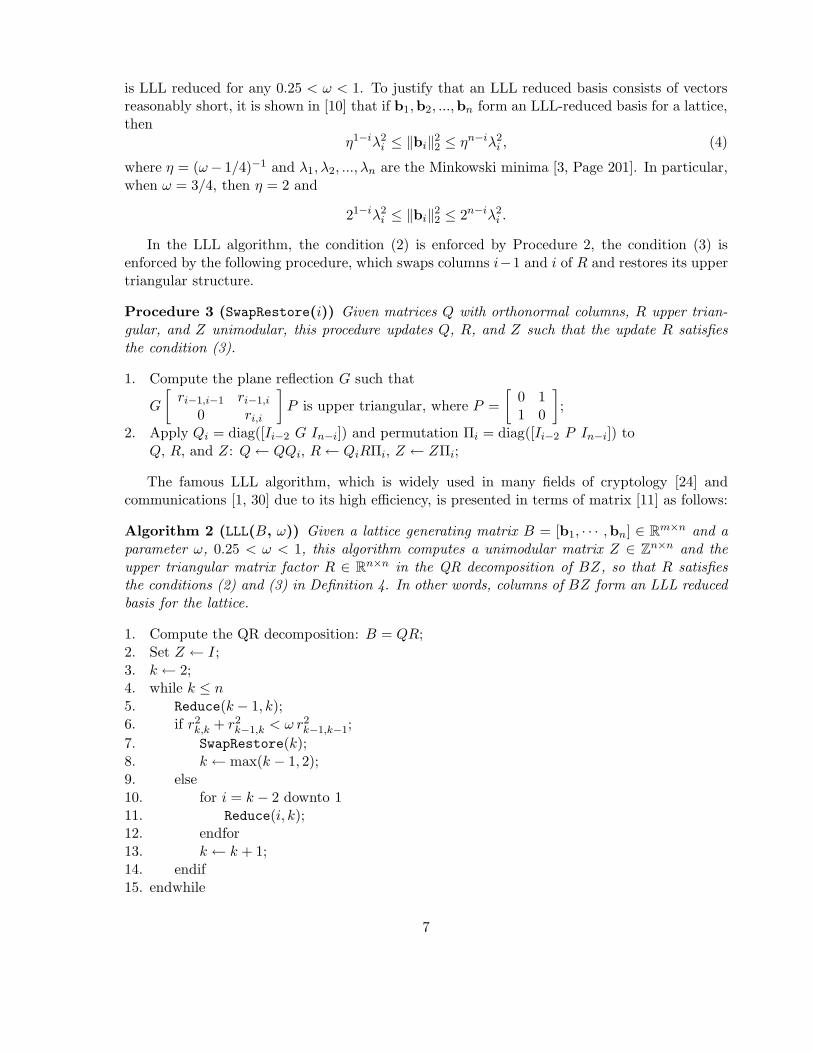
is LLL reduced for any 0.25 < ω < 1. To justify that an LLL reduced basis consists of vectorsreasonably short, it is shown in [10] that if b1,b2, ...,bn form an LLL-reduced basis for a lattice,then

η1−iλ2i ≤ ‖bi‖

22 ≤ ηn−iλ2

i , (4)

where η = (ω− 1/4)−1 and λ1, λ2, ..., λn are the Minkowski minima [3, Page 201]. In particular,when ω = 3/4, then η = 2 and

21−iλ2i ≤ ‖bi‖

22 ≤ 2n−iλ2

i .

In the LLL algorithm, the condition (2) is enforced by Procedure 2, the condition (3) isenforced by the following procedure, which swaps columns i−1 and i of R and restores its uppertriangular structure.

Procedure 3 (SwapRestore(i)) Given matrices Q with orthonormal columns, R upper trian-gular, and Z unimodular, this procedure updates Q, R, and Z such that the update R satisfiesthe condition (3).

1. Compute the plane reflection G such that

G

[

ri−1,i−1 ri−1,i

0 ri,i

]

P is upper triangular, where P =

[

0 11 0

]

;

2. Apply Qi = diag([Ii−2 G In−i]) and permutation Πi = diag([Ii−2 P In−i]) toQ, R, and Z: Q← QQi, R← QiRΠi, Z ← ZΠi;

The famous LLL algorithm, which is widely used in many fields of cryptology [24] andcommunications [1, 30] due to its high efficiency, is presented in terms of matrix [11] as follows:

Algorithm 2 (LLL(B, ω)) Given a lattice generating matrix B = [b1, · · · ,bn] ∈ Rm×n and aparameter ω, 0.25 < ω < 1, this algorithm computes a unimodular matrix Z ∈ Zn×n and theupper triangular matrix factor R ∈ Rn×n in the QR decomposition of BZ, so that R satisfiesthe conditions (2) and (3) in Definition 4. In other words, columns of BZ form an LLL reducedbasis for the lattice.

1. Compute the QR decomposition: B = QR;2. Set Z ← I;3. k ← 2;4. while k ≤ n5. Reduce(k − 1, k);6. if r2

k,k + r2k−1,k < ω r2

k−1,k−1;

7. SwapRestore(k);8. k ← max(k − 1, 2);9. else10. for i = k − 2 downto 111. Reduce(i, k);12. endfor13. k ← k + 1;14. endif15. endwhile

7

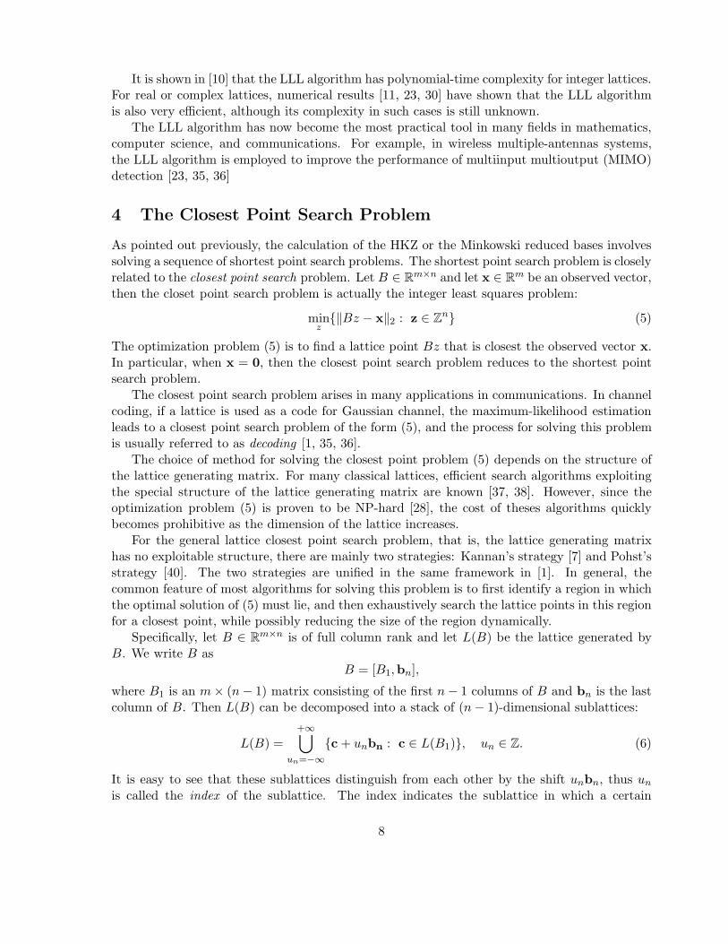
It is shown in [10] that the LLL algorithm has polynomial-time complexity for integer lattices.For real or complex lattices, numerical results [11, 23, 30] have shown that the LLL algorithmis also very efficient, although its complexity in such cases is still unknown.

The LLL algorithm has now become the most practical tool in many fields in mathematics,computer science, and communications. For example, in wireless multiple-antennas systems,the LLL algorithm is employed to improve the performance of multiinput multioutput (MIMO)detection [23, 35, 36]

4 The Closest Point Search Problem

As pointed out previously, the calculation of the HKZ or the Minkowski reduced bases involvessolving a sequence of shortest point search problems. The shortest point search problem is closelyrelated to the closest point search problem. Let B ∈ Rm×n and let x ∈ Rm be an observed vector,then the closet point search problem is actually the integer least squares problem:

minz{‖Bz − x‖2 : z ∈ Zn} (5)

The optimization problem (5) is to find a lattice point Bz that is closest the observed vector x.In particular, when x = 0, then the closest point search problem reduces to the shortest pointsearch problem.

The closest point search problem arises in many applications in communications. In channelcoding, if a lattice is used as a code for Gaussian channel, the maximum-likelihood estimationleads to a closest point search problem of the form (5), and the process for solving this problemis usually referred to as decoding [1, 35, 36].

The choice of method for solving the closest point problem (5) depends on the structure ofthe lattice generating matrix. For many classical lattices, efficient search algorithms exploitingthe special structure of the lattice generating matrix are known [37, 38]. However, since theoptimization problem (5) is proven to be NP-hard [28], the cost of theses algorithms quicklybecomes prohibitive as the dimension of the lattice increases.

For the general lattice closest point search problem, that is, the lattice generating matrixhas no exploitable structure, there are mainly two strategies: Kannan’s strategy [7] and Pohst’sstrategy [40]. The two strategies are unified in the same framework in [1]. In general, thecommon feature of most algorithms for solving this problem is to first identify a region in whichthe optimal solution of (5) must lie, and then exhaustively search the lattice points in this regionfor a closest point, while possibly reducing the size of the region dynamically.

Specifically, let B ∈ Rm×n is of full column rank and let L(B) be the lattice generated byB. We write B as

B = [B1,bn],

where B1 is an m× (n− 1) matrix consisting of the first n− 1 columns of B and bn is the lastcolumn of B. Then L(B) can be decomposed into a stack of (n− 1)-dimensional sublattices:

L(B) =

+∞⋃

un=−∞

{c + unbn : c ∈ L(B1)}, un ∈ Z. (6)

It is easy to see that these sublattices distinguish from each other by the shift unbn, thus un

is called the index of the sublattice. The index indicates the sublattice in which a certain

8

lattice point lies. Denote b⊥ the orthogonal projection of bn on the orthogonal complementarysubspace R(B1)

⊥ of the range space R(B1) of B1. Then a sublattice with index un is containedin a subspace Sun

defined by

Sun= {v + unb⊥ : v ∈ R(B1)} (7)

Let x ∈ Rm be the observed vector to be decoded in the lattice L(B). The orthogonal distancefrom x to the subspace Sun

is

d(x, Sun) = |un − un| · ‖b⊥‖2, where un =

xTb⊥

‖b⊥‖22

. (8)

Let x denote the closest lattice point to x, and suppose that x lies in a sublattice St defined in(6) with index t ∈ Z. If an upper bound ρn on ‖x− x‖2 is given, then

d(x, St) ≤ ρn. (9)

From (8) and (9), x must lie in one of the sublattices indexed by

un =

⌈

un −ρn

‖b⊥‖2

⌉

, . . . ,

⌊

un +ρn

‖b⊥‖2

⌋

, (10)

a finite sequence of consecutive integers. Therefore, an n-dimensional closest point search prob-lem can be reduced to a finite number of (n − 1)-dimensional closest point search problems,leading to a recursive method for solving the problem (5). In summary, we present the followingpseudo code for solving the closest point search problem.

Algorithm 3 (Decode(B,x)) Given a matrix B ∈ Rm×n (m ≥ n) of full column rank and avector x ∈ Rm, this algorithm computes a solution of the closest point search problem (5).

1. if m = 12. return z = ⌊ x

B⌉;

3. else4. Determine an initial size ρn of the search region;5. Compute b⊥ defined previously and un in (8);6. For each index un in (10), solve the (n− 1)-dimensional

closest point search problemwun

= Decode(B1,x− unb⊥ − unb)in a search region with an updated size ρn−1;

7. For each index un in (10), construct zun= [wun

un]T, find zminimizing ‖Bzun

− x‖2, and return z.

There are various implementations of Algorithm 3. The main differences among them havethe following three aspects:

• The choice of the initial size ρn of search region. The most algorithms based on the Kannanstrategy [7, 17, 8, 27] or the Phost strategy [39, 40, 41] take the distance between x and thefirst column of the lattice generating matrix as the initial size. A better choice is the Babai

9

nearest point [42], which is usually closer to x than the first column of the lattice generatingmatrix. The most algorithms based on the Schnorr-Euchner strategy [26, 1] take thedistance between x and the Babai nearest point as the initial size. Furthermore, algorithmsbased on the Phost or the Schnorr-Euchner strategy reduce the size ρn dynamically toimprove their performance. That is, when any lattice point x′ inside the search region isfound, the bound ρn can be reduced to ‖x′ − x‖2, since ‖x′ − x‖2 ≤ ρn. The algorithmsbased on the Kannan strategy scan all the (n − 1)-dimensional sublattices with the samevalue of ρn.

• The choice of the updated upper bound ρn−1. Generally, the algorithms based on theKannan strategy search all the sublattices with indices in (10) using the same value of ρn−1.The methods in [7], [17], [8], and [27] differ from each other mainly on how the updatedbounds ρk, k = 1, ..., n, are chosen. The algorithms based on the Phost [39, 40, 41] orthe Schnorr-Euchner [26, 1] strategy update ρn−1 =

√

ρ2n − d(x, Sun

)2, which differs fromsublattice to sublattice. Geometrically, the lattice points inside a hypersphere are searched.

• The order in which the sublattices are examined. The algorithms based on the Kannan orthe Phost strategy scan all the (n−1)-dimensional sublattices with indices in (10) followinga natural order. Assuming that un ≤ ⌊un⌉, the algorithms based on the Schnorr-Euchnerstrategy [26, 1] search sublattices with indices following the alternating order:

un = ⌊un⌉, ⌊un⌉ − 1, ⌊un⌉+ 1, ⌊un⌉ − 2, . . . . (11)

The order in (11) is obtained according to nondecreasing distances d(x, Sun). By using

this search order, the chance of finding the correct sublattice early is maximized. So thealgorithms based on the Schnorr-Euchner strategy are usually more efficient than thosebased on the Kannan or the Phost stategy.

In addition to the above three aspects, the structure of the given lattice generating matrixalso has a significant impact on the efficiency of the decoding algorithm. All the algorithmsmentioned above usually use the LLL algorithm as a preprocessor, since the performance of thedecoding algorithm can be further improved for the LLL reduced bases. For applications wherethe same lattice is searched many times, a better choice is to use the HKZ reduction algorithmas a preprocessor [1].

5 A New Algorithm for Constructing the HKZ Reduced Bases

In 1983, Kannan [7] proposed the first algorithm for constructing the HKZ reduced bases for gen-eral lattices. Based on Kannan strategy, Helfrich [17], Kannan [8], and Banihashemi and Khan-dani [27] further refined Kannan’s algorithm. All the algorithms based on the Kannan strategyare intended as theoretical results rather than practical tools, since the induction conditionsimposed by the Kannan strategy are crucial and the complexity quickly becomes prohibitive asthe dimension of lattices increases.

From Definition 2, the key to the construction of an HKZ reduced basis is to recursivelyfind a shortest nonzero lattice vector and then to extend this vector to a basis for the lattice.From Section 4, the Schnorr-Euchner strategy is currently the most efficient method for finding

10

a shortest nonzero lattice point. Agrell et al. [1] presented a practical implementation of theSchnorr-Euchner strategy and combine their sphere decoding algorithm with the Kannan’s basisexpansion algorithm to construct an HKZ reduced basis for a given lattice.

In this section, we present a new algorithm for computing the HKZ reduced bases for generallattices. In our algorithm, we adopt the sphere decoding method in [1] to compute a shortestnonzero lattice vector. However, instead of the Kannan’s basis expansion method used in [1],we use a novel unimodular transformation basis expansion strategy.

Firstly, we state the Kannan’s basis expansion method.

Algorithm 4 (SELECT-BASIS(n; b1, · · · ,bn+1)[8]) Suppose that b1, · · · ,bn+1 are vectors inQm for some m ≥ n and span an n-dimensional lattice L of Qm. This procedure returns a basis{a1, · · · ,an} for L, where a1 is a shortest lattice vector in the direction of b1.

1. if n = 0 or b1 = 0 then do the obvious;2. if b1 is independent of b2, · · · ,bn+1

3. a1 ← b1;4. else

5. Find the rationals α2, · · · , αn+1 (unique) such that∑n+1

j=2 αjbj = b1;

6. M ← least common multiples of the denominators of α2, · · · , αn+1;7. γ ← gcd(Mα2, · · · ,Mαn+1);8. Let M/γ = p/q, where p, q are relatively prime integers. a1 ← (1/q)b1;9. endif

10. bi ← bi −〈bi,a1〉〈a1,a1〉

a1, i = 2, · · · , n + 1;

11. (c2, · · · , cn)← SELECT-BASIS(n− 1;b2, · · · ,bn+1);12. Lift ci to ai in L for i = 2, · · · , n and return (a1, · · · ,an).

Secondly, we give a brief complexity analysis of Algorithm 4. Step 11 shows that the algo-rithm is recursive and each time the problem size is reduced by one, from n downto 1. In eachrecursion, the major cost is in steps 2 and 5, which involve solving systems of linear equationsrequiring O(k3) arithmetic operations, assuming the k is the problem size in the recursion. Thusthe complexity of Algorithm 4 is O(n4) (O(

∑nk=1 k3)). Moreover, note that Algorithm 4 only

works for rational lattices, not general real lattices.We propose a basis expansion method based on the unimodular transformation presented

in [33], which is applicable for general real or complex lattices. Specifically, let B ∈ Rm×n bea matrix generating the lattice L. Suppose that Bz is a shortest nonzero point of L, wherez = [zi] ∈ Zn. Then the problem of expanding Bz to a basis of L is equivalent to the problemof constructing an n-by-n unimodular matrix Z whose first column is z, because the columnsof BZ form a basis for L. In other words, Z−1z = e1, which says that Z−1, also unimodular,transforms z into the first unit vector e1.

For the special case when n = 2, we have the following algorithm:

Procedure 4 (Unim2(p, q)[33]) Let [p q]T be a nonzero integer vector and gcd(p, q) = d. Usingthe extended Euclidean algorithm, find integers a and b such that ap+bq = d. The integer matrix

M =

[

p/d −bq/d a

]

, (12)

11

is unimodular and

M−1

[

pq

]

=

[

d0

]

, M−1 =

[

a b−q/d p/d

]

.

The above procedure shows that given a nonzero integer vector [p q]T, gcd(p, q) = d, we canconstruct an integer unimodular matrix (12) whose inverse can be applied to [p q]T to annihilateits second entry. In particular, if gcd(p, q) = ±1, then [p q]T can be transformed into the firstunit vector.

Now we consider the general case when n > 2. Since Bz is a shortest nonzero lattice point,we have gcd(zi) = ±1, implying that a sequence of the plane unimodular transformations Mdescribed above can be applied to transform z into the first unit vector.

As pointed out earlier, the construction of an HKZ reduced basis involves the shortest latticevector search problem and we adopt the sphere decoding method. Since the LLL algorithmintroduced in Section 3 can significantly accelerate the search process of the sphere decodingalgorithm [1], we use the LLL algorithm as a preprocessor.

Putting all things together, we present our new algorithm for constructing an HKZ reducedbasis.

Algorithm 5 (LLL-aid-HKZ-red(B, w)) Given a lattice generator matrix B ∈ Rm×n and aparameter ω, where 0.25 < ω < 1, this algorithm computes a unimodular matrix Z ∈ Zn×n suchthat the columns of BZ form an HKZ reduced basis.

1. Compute the QR decomposition: B = QR;2. Z ← In;3. for k = 1 to n− 14. Apply the LLL algorithm to R(k : n, k : n);5. Use the sphere decoding algorithm [1] to find a nonzero vector z ∈ Zn−k+1 so that

R(k : n, k : n)z is a shortest point in the lattice generated by R(k : n, k : n);6. Transform(k, z);7. endfor8. for j = 2 to n9. for i = j − 1 downto 110. Reduce(i, j);11. endfor12. endfor

The procedure Transform in line 6 expands the shortest nonzero lattice vector found in line 5to a basis for the n−k+1-dimensional lattice generated by the trailing submatrix R(k : n, k : n) ofR using Procedure 4. Moreover, since the LLL algorithm is incorporated into the algorithm, thisprocedure should also maintain the upper triangular structure of R and update the unimodularmatrix Z. The following is an implementation of the procedure.

Procedure 5 (Transform(k, z)[33]) Given R ∈ Rn×n upper triangular, Z ∈ Zn×n unimodular,and an integer vector z ∈ Zn−k+1, 1 ≤ k ≤ n− 1, such that gcd(zi) = ±1,

12

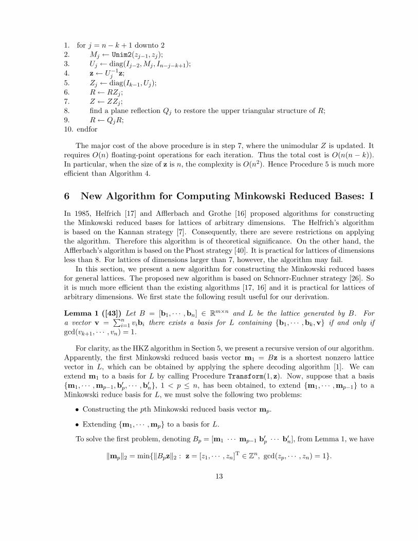
1. for j = n− k + 1 downto 22. Mj ← Unim2(zj−1, zj);3. Uj ← diag(Ij−2,Mj , In−j−k+1);

4. z← U−1j z;

5. Zj ← diag(Ik−1, Uj);6. R← RZj ;7. Z ← ZZj;8. find a plane reflection Qj to restore the upper triangular structure of R;9. R← QjR;10. endfor

The major cost of the above procedure is in step 7, where the unimodular Z is updated. Itrequires O(n) floating-point operations for each iteration. Thus the total cost is O(n(n − k)).In particular, when the size of z is n, the complexity is O(n2). Hence Procedure 5 is much moreefficient than Algorithm 4.

6 New Algorithm for Computing Minkowski Reduced Bases: I

In 1985, Helfrich [17] and Afflerbach and Grothe [16] proposed algorithms for constructingthe Minkowski reduced bases for lattices of arbitrary dimensions. The Helfrich’s algorithmis based on the Kannan strategy [7]. Consequently, there are severe restrictions on applyingthe algorithm. Therefore this algorithm is of theoretical significance. On the other hand, theAfflerbach’s algorithm is based on the Phost strategy [40]. It is practical for lattices of dimensionsless than 8. For lattices of dimensions larger than 7, however, the algorithm may fail.

In this section, we present a new algorithm for constructing the Minkowski reduced basesfor general lattices. The proposed new algorithm is based on Schnorr-Euchner strategy [26]. Soit is much more efficient than the existing algorithms [17, 16] and it is practical for lattices ofarbitrary dimensions. We first state the following result useful for our derivation.

Lemma 1 ([43]) Let B = [b1, · · · ,bn] ∈ Rm×n and L be the lattice generated by B. Fora vector v =

∑ni=1 vibi there exists a basis for L containing {b1, · · · ,bk,v} if and only if

gcd(vk+1, · · · , vn) = 1.

For clarity, as the HKZ algorithm in Section 5, we present a recursive version of our algorithm.Apparently, the first Minkowski reduced basis vector m1 = Bz is a shortest nonzero latticevector in L, which can be obtained by applying the sphere decoding algorithm [1]. We canextend m1 to a basis for L by calling Procedure Transform(1, z). Now, suppose that a basis{m1, · · · ,mp−1,b

′p, · · · ,b

′n}, 1 < p ≤ n, has been obtained, to extend {m1, · · · ,mp−1} to a

Minkowski reduce basis for L, we must solve the following two problems:

• Constructing the pth Minkowski reduced basis vector mp.

• Extending {m1, · · · ,mp} to a basis for L.

To solve the first problem, denoting Bp = [m1 · · · mp−1 b′p · · · b′

n], from Lemma 1, we have

‖mp‖2 = min{‖Bpz‖2 : z = [z1, · · · , zn]T ∈ Zn, gcd(zp, · · · , zn) = 1}.

13

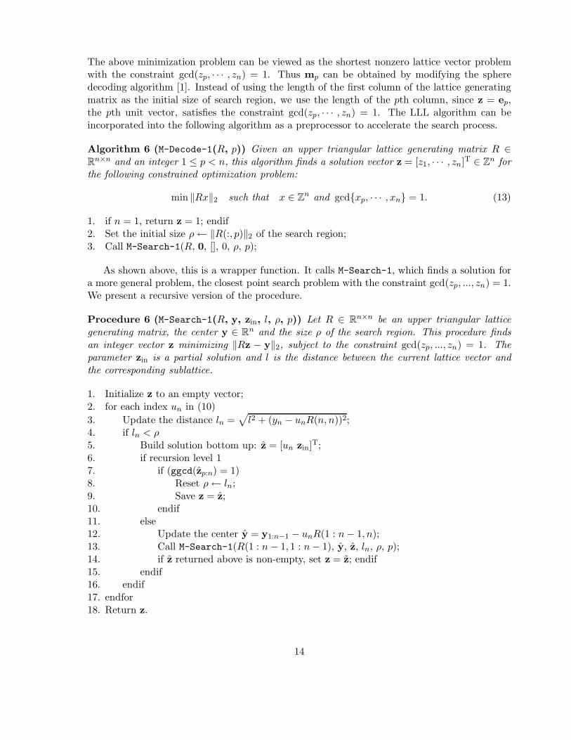
The above minimization problem can be viewed as the shortest nonzero lattice vector problemwith the constraint gcd(zp, · · · , zn) = 1. Thus mp can be obtained by modifying the spheredecoding algorithm [1]. Instead of using the length of the first column of the lattice generatingmatrix as the initial size of search region, we use the length of the pth column, since z = ep,the pth unit vector, satisfies the constraint gcd(zp, · · · , zn) = 1. The LLL algorithm can beincorporated into the following algorithm as a preprocessor to accelerate the search process.

Algorithm 6 (M-Decode-1(R, p)) Given an upper triangular lattice generating matrix R ∈Rn×n and an integer 1 ≤ p < n, this algorithm finds a solution vector z = [z1, · · · , zn]T ∈ Zn forthe following constrained optimization problem:

min ‖Rx‖2 such that x ∈ Zn and gcd{xp, · · · , xn} = 1. (13)

1. if n = 1, return z = 1; endif2. Set the initial size ρ← ‖R(:, p)‖2 of the search region;3. Call M-Search-1(R, 0, [], 0, ρ, p);

As shown above, this is a wrapper function. It calls M-Search-1, which finds a solution fora more general problem, the closest point search problem with the constraint gcd(zp, ..., zn) = 1.We present a recursive version of the procedure.

Procedure 6 (M-Search-1(R, y, zin, l, ρ, p)) Let R ∈ Rn×n be an upper triangular latticegenerating matrix, the center y ∈ Rn and the size ρ of the search region. This procedure findsan integer vector z minimizing ‖Rz − y‖2, subject to the constraint gcd(zp, ..., zn) = 1. Theparameter zin is a partial solution and l is the distance between the current lattice vector andthe corresponding sublattice.

1. Initialize z to an empty vector;2. for each index un in (10)

3. Update the distance ln =√

l2 + (yn − unR(n, n))2;4. if ln < ρ5. Build solution bottom up: z = [un zin]T;6. if recursion level 17. if (ggcd(zp:n) = 1)8. Reset ρ← ln;9. Save z = z;10. endif11. else12. Update the center y = y1:n−1 − unR(1 : n− 1, n);13. Call M-Search-1(R(1 : n− 1, 1 : n− 1), y, z, ln, ρ, p);14. if z returned above is non-empty, set z = z; endif15. endif16. endif17. endfor18. Return z.

14

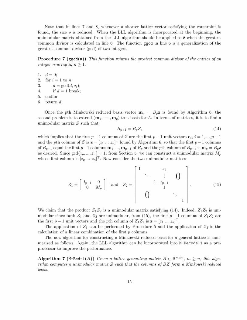
Note that in lines 7 and 8, whenever a shorter lattice vector satisfying the constraint isfound, the size ρ is reduced. When the LLL algorithm is incorporated at the beginning, theunimodular matrix obtained from the LLL algorithm should be applied to z when the greatestcommon divisor is calculated in line 6. The function ggcd in line 6 is a generalization of thegreatest common divisor (gcd) of two integers.

Procedure 7 (ggcd(a)) This function returns the greatest common divisor of the entries of aninteger n-array a, n ≥ 1.

1. d = 0;2. for i = 1 to n3. d = gcd(d, ai);4. if d = 1 break;5. endfor6. return d.

Once the pth Minkowski reduced basis vector mp = Bpz is found by Algorithm 6, thesecond problem is to extend (m1, · · · ,mp) to a basis for L. In terms of matrices, it is to find aunimodular matrix Z such that

Bp+1 = BpZ, (14)

which implies that the first p− 1 columns of Z are the first p− 1 unit vectors ei, i = 1, ..., p− 1and the pth column of Z is z = [z1 ... zn]T found by Algorithm 6, so that the first p− 1 columnsof Bp+1 equal the first p−1 columns m1, ...,mp−1 of Bp and the pth column of Bp+1 is mp = Bpzas desired. Since gcd(zp, ..., zn) = 1, from Section 5, we can construct a unimodular matrix Mp

whose first column is [zp ... zn]T. Now consider the two unimodular matrices

Z1 =

[

Ip−1 00 Mp

]

and Z2 =

1 z1

. . ....

1 zp−1

01

. . .01

. (15)

We claim that the product Z1Z2 is a unimodular matrix satisfying (14). Indeed, Z1Z2 is uni-modular since both Z1 and Z2 are unimodular, from (15), the first p − 1 columns of Z1Z2 arethe first p− 1 unit vectors and the pth column of Z1Z2 is z = [z1 ... zn]T.

The application of Z1 can be performed by Procedure 5 and the application of Z2 is thecalculation of a linear combination of the first p columns.

The new algorithm for constructing a Minkowski reduced basis for a general lattice is sum-marized as follows. Again, the LLL algorithm can be incorporated into M-Decode-1 as a pre-processor to improve the performance.

Algorithm 7 (M-Red-1(B)) Given a lattice generating matrix B ∈ Rm×n, m ≥ n, this algo-rithm computes a unimodular matrix Z such that the columns of BZ form a Minkowski reducedbasis.

15

1. QR decomposition: B = QR;2. Z ← In;3. for k = 1 to n4. Call M-Decode-1(R, k) to find the solution z for (13);5. Call Transform(k, [zk, · · · , zn]T) to apply Z1 in (15);6. Apply Z2 in (15) to R:

R(1 : k − 1, k)← R(1 : k − 1, k) + R(1 : k − 1, 1 : k − 1)[z1, · · · , zk−1]T.

7. Apply Z2 to Z:Z(:, k)← Z(:, k) + Z(:, 1 : k − 1)[z1, · · · , zk−1]

T.8. endfor

7 New Algorithm for Computing Minkowski Reduced Bases: II

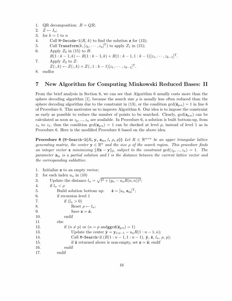
From the brief analysis in Section 6, we can see that Algorithm 6 usually costs more than thesphere decoding algorithm [1], because the search size ρ is usually less often reduced than thesphere decoding algorithm due to the constraint in (13), or the condition gcd(zp:n) = 1 in line 6of Procedure 6. This motivates us to improve Algorithm 6. Our idea is to impose the constraintas early as possible to reduce the number of points to be searched. Clearly, gcd(zp:n) can becalculated as soon as zp, ..., zn are available. In Procedure 6, a solution is built bottom-up, fromzn to z1, thus the condition gcd(zp:n) = 1 can be checked at level p, instead of level 1 as inProcedure 6. Here is the modified Procedure 6 based on the above idea.

Procedure 8 (M-Search-2(R, y, zin, l, ρ, p)) Let R ∈ Rn×n be an upper triangular latticegenerating matrix, the center y ∈ Rn and the size ρ of the search region. This procedure findsan integer vector z minimizing ‖Rz − y‖2, subject to the constraint gcd(zp, ..., zn) = 1. Theparameter zin is a partial solution and l is the distance between the current lattice vector andthe corresponding sublattice.

1. Initialize z to an empty vector;2. for each index un in (10)

3. Update the distance ln =√

l2 + (yn − unR(n, n))2;4. if ln < ρ5. Build solution bottom up: z = [un zin]

T;6. if recursion level 17. if (ln > 0)8. Reset ρ← ln;9. Save z = z;10. endif11 else12. if (n 6= p) or (n = p andggcd(zp:n) = 1)13. Update the center y = y1:n−1 − unR(1 : n− 1, n);14. Call M-Search-2 (R(1 : n− 1, 1 : n− 1), y, z, ln, ρ, p);15. if z returned above is non-empty, set z = z; endif16. endif17. endif

16

18. endif19. endfor20. Return z.

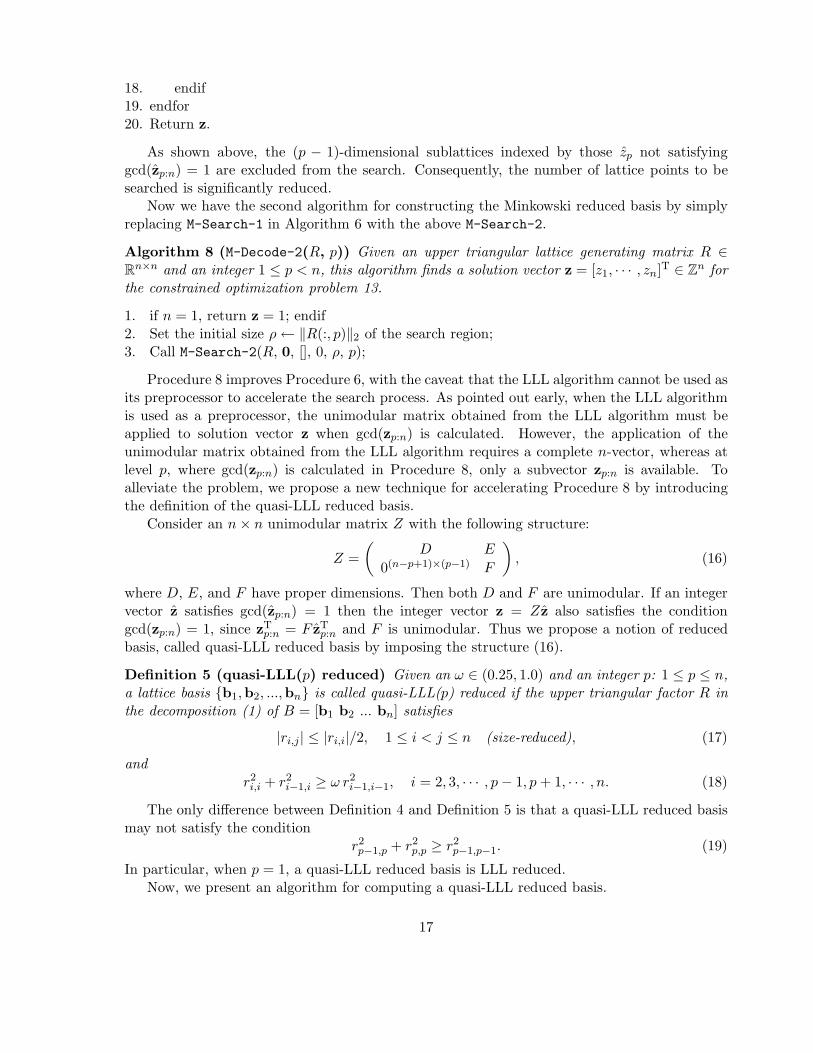
As shown above, the (p − 1)-dimensional sublattices indexed by those zp not satisfyinggcd(zp:n) = 1 are excluded from the search. Consequently, the number of lattice points to besearched is significantly reduced.

Now we have the second algorithm for constructing the Minkowski reduced basis by simplyreplacing M-Search-1 in Algorithm 6 with the above M-Search-2.

Algorithm 8 (M-Decode-2(R, p)) Given an upper triangular lattice generating matrix R ∈Rn×n and an integer 1 ≤ p < n, this algorithm finds a solution vector z = [z1, · · · , zn]T ∈ Zn forthe constrained optimization problem 13.

1. if n = 1, return z = 1; endif2. Set the initial size ρ← ‖R(:, p)‖2 of the search region;3. Call M-Search-2(R, 0, [], 0, ρ, p);

Procedure 8 improves Procedure 6, with the caveat that the LLL algorithm cannot be used asits preprocessor to accelerate the search process. As pointed out early, when the LLL algorithmis used as a preprocessor, the unimodular matrix obtained from the LLL algorithm must beapplied to solution vector z when gcd(zp:n) is calculated. However, the application of theunimodular matrix obtained from the LLL algorithm requires a complete n-vector, whereas atlevel p, where gcd(zp:n) is calculated in Procedure 8, only a subvector zp:n is available. Toalleviate the problem, we propose a new technique for accelerating Procedure 8 by introducingthe definition of the quasi-LLL reduced basis.

Consider an n× n unimodular matrix Z with the following structure:

Z =

(

D E

0(n−p+1)×(p−1) F

)

, (16)

where D, E, and F have proper dimensions. Then both D and F are unimodular. If an integervector z satisfies gcd(zp:n) = 1 then the integer vector z = Zz also satisfies the conditiongcd(zp:n) = 1, since zT

p:n = F zTp:n and F is unimodular. Thus we propose a notion of reduced

basis, called quasi-LLL reduced basis by imposing the structure (16).

Definition 5 (quasi-LLL(p) reduced) Given an ω ∈ (0.25, 1.0) and an integer p: 1 ≤ p ≤ n,a lattice basis {b1,b2, ...,bn} is called quasi-LLL(p) reduced if the upper triangular factor R inthe decomposition (1) of B = [b1 b2 ... bn] satisfies

|ri,j| ≤ |ri,i|/2, 1 ≤ i < j ≤ n (size-reduced), (17)

andr2i,i + r2

i−1,i ≥ ω r2i−1,i−1, i = 2, 3, · · · , p− 1, p + 1, · · · , n. (18)

The only difference between Definition 4 and Definition 5 is that a quasi-LLL reduced basismay not satisfy the condition

r2p−1,p + r2

p,p ≥ r2p−1,p−1. (19)

In particular, when p = 1, a quasi-LLL reduced basis is LLL reduced.Now, we present an algorithm for computing a quasi-LLL reduced basis.

17

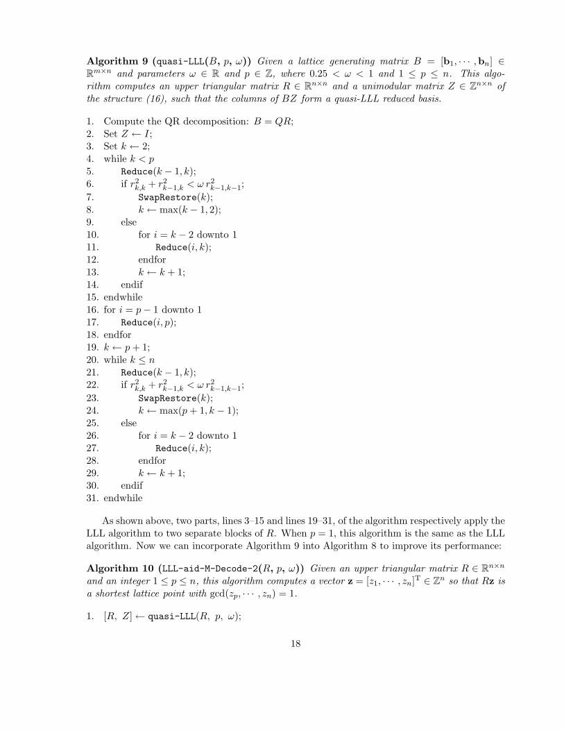
Algorithm 9 (quasi-LLL(B, p, ω)) Given a lattice generating matrix B = [b1, · · · ,bn] ∈Rm×n and parameters ω ∈ R and p ∈ Z, where 0.25 < ω < 1 and 1 ≤ p ≤ n. This algo-rithm computes an upper triangular matrix R ∈ Rn×n and a unimodular matrix Z ∈ Zn×n ofthe structure (16), such that the columns of BZ form a quasi-LLL reduced basis.

1. Compute the QR decomposition: B = QR;2. Set Z ← I;3. Set k ← 2;4. while k < p5. Reduce(k − 1, k);6. if r2

k,k + r2k−1,k < ω r2

k−1,k−1;

7. SwapRestore(k);8. k ← max(k − 1, 2);9. else10. for i = k − 2 downto 111. Reduce(i, k);12. endfor13. k ← k + 1;14. endif15. endwhile16. for i = p− 1 downto 117. Reduce(i, p);18. endfor19. k ← p + 1;20. while k ≤ n21. Reduce(k − 1, k);22. if r2

k,k + r2k−1,k < ω r2

k−1,k−1;

23. SwapRestore(k);24. k ← max(p + 1, k − 1);25. else26. for i = k − 2 downto 127. Reduce(i, k);28. endfor29. k ← k + 1;30. endif31. endwhile

As shown above, two parts, lines 3–15 and lines 19–31, of the algorithm respectively apply theLLL algorithm to two separate blocks of R. When p = 1, this algorithm is the same as the LLLalgorithm. Now we can incorporate Algorithm 9 into Algorithm 8 to improve its performance:

Algorithm 10 (LLL-aid-M-Decode-2(R, p, ω)) Given an upper triangular matrix R ∈ Rn×n

and an integer 1 ≤ p ≤ n, this algorithm computes a vector z = [z1, · · · , zn]T ∈ Zn so that Rz isa shortest lattice point with gcd(zp, · · · , zn) = 1.

1. [R, Z]← quasi-LLL(R, p, ω);

18

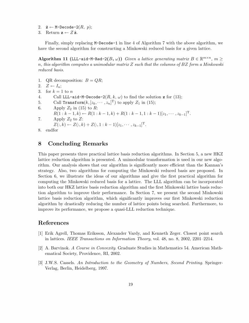
2. z← M-Decode-2(R, p);3. Return z← Z z.

Finally, simply replacing M-Decode-1 in line 4 of Algorithm 7 with the above algorithm, wehave the second algorithm for constructing a Minkowski reduced basis for a given lattice.

Algorithm 11 (LLL-aid-M-Red-2(B, ω)) Given a lattice generating matrix B ∈ Rm×n, m ≥n, this algorithm computes a unimodular matrix Z such that the columns of BZ form a Minkowskireduced basis.

1. QR decomposition: B = QR;2. Z ← In;3. for k = 1 to n4. Call LLL-aid-M-Decode-2(R, k, ω) to find the solution z for (13);5. Call Transform(k, [zk, · · · , zn]T) to apply Z1 in (15);6. Apply Z2 in (15) to R:

R(1 : k − 1, k)← R(1 : k − 1, k) + R(1 : k − 1, 1 : k − 1)[z1, · · · , zk−1]T.

7. Apply Z2 to Z:Z(:, k)← Z(:, k) + Z(:, 1 : k − 1)[z1, · · · , zk−1]

T.8. endfor

8 Concluding Remarks

This paper presents three practical lattice basis reduction algorithms. In Section 5, a new HKZlattice reduction algorithm is presented. A unimodular transformation is used in our new algo-rithm. Our analysis shows that our algorithm is significantly more efficient than the Kannan’sstrategy. Also, two algorithms for computing the Minkowski reduced basis are proposed. InSection 6, we illustrate the ideas of our algorithms and give the first practical algorithm forcomputing the Minkowski reduced basis for a lattice. The LLL algorithm can be incorporatedinto both our HKZ lattice basis reduction algorithm and the first Minkowski lattice basis reduc-tion algorithm to improve their performance. In Section 7, we present the second Minkowskilattice basis reduction algorithm, which significantly improves our first Minkowski reductionalgorithm by drastically reducing the number of lattice points being searched. Furthermore, toimprove its performance, we propose a quasi-LLL reduction technique.

References

[1] Erik Agrell, Thomas Eriksson, Alexander Vardy, and Kenneth Zeger. Closest point searchin lattices. IEEE Transactions on Information Theory, vol. 48, no. 8, 2002, 2201–2214.

[2] A. Barvinok. A Course in Convexity. Graduate Studies in Mathematics 54. American Math-ematical Society, Providence, RI, 2002.

[3] J.W.S. Cassels. An Introduction to the Geometry of Numbers, Second Printing. Springer-Verlag, Berlin, Heidelberg, 1997.

19

[4] H. Cohen. A Course in Computational Algebraic Number Theory. Graduate Texts in Math-ematics 138, Second corrected printing. Springer, Berlin, 1995.

[5] G.H. Golub and C.F. Van Loan. Matrix Computations, Third Edition. The Johns HopkinsUniversity Press, Baltimore, MD, 1996.

[6] A. Joux and J. Stern. Lattice reduction: A toolbox for the cryptanalyst. Journal of Cryp-tology, 11(3), 1998, 161–185.

[7] Ravi Kannan. Improved algorithms for integer programming and related lattice problems.Proc. ACM Symp. Theory of Computing, Boston, MA, Apr, 1983, 193–206.

[8] Ravi Kannan. Minkowski’s convex body theorem and integer programming. Mathematics ofOperations Research, 3(12), 1987, 415–440.

[9] A. Korkine and G. Zolotareff. Sur les formes quadratiques. Maht. Ann., 6, 1873, 366–389.

[10] A.K. Lenstra, H.W. Lenstra, Jr. and L. Lovasz. Factorizing polynomials with rational co-efficients. Mathematicsche Annalen, 261, 1982, 515–534.

[11] F.T. Luk and D.M. Tracy. An improved LLL algorithm. Linear Algebra and its Applications,428(2–3), 2008, 441–452.

[12] H. Minkowski. Geometrie der Zahlen. Teubner, Leipzig, 1896.

[13] The LLL Algorithm: Survey and Applications. Information Security and Cryptography,Texts and Monographs. Editors Phong Q. Nguyen and Brigitte Vallee. Springer HeidelbergDordrecht London New York, 2010.

[14] H. Minkowski. Uber die positiven quadratischen Formen und uber kettenbruchahnlicheAlgorithmen. Journal fur die Reine und Angewandte Mathematik, vol. 107, 1891, 278–297.

[15] J. C. Lagarias. Worst-case complexity bounds for algorithms in the theory of integralquadratic forms. J. Algorithms, 1, 1980, 142–186.

[16] L. Afflerbach and H. Grothe. Calculation of Minkowski-reduced lattice bases. Computing,vol. 35, no. 3-4, 1985, 269–276.

[17] Bettina Helfrich. Algorithms to construct Minkowski reduced and Hermite reduced latticebases. Theoretical Computer Science, vol. 41, no. 2-3, 1985, 125–139.

[18] D. E. Knuth. The Art of Computer Programming, 2nd ed. Reading, MA: Addison-Wesley,1981, vol. 2.

[19] G. Marsaglia. The structure of linear congruential sequences. Applications of Number The-ory to Numerical Analysis (S. K. Zaremba, ed), 1972, 249-285.

[20] W. A. Beyer, R. B. Roof, and D. Williamson. The lattice structure of multiplicative con-gruential pseudo-random vectors. Math. Comput, 25, 1971, 345-360.

[21] M. Grotschel, L. Lovasz, and A. Schrijver. Geometric Algorithms and Combinatorial Opti-mization, Spriger, Berlin, 1993.

20

[22] D. Micciancio and S. Goldwasser. Complexity of Lattice Problems: A Cryptographic Perspec-tive, Kluwer Internat. Ser. Engrg. Comput. Sci. 671, Kluwer Academic Publishers, Boston,MA, 2002.

[23] Y. H. Gan, C. Ling, and H. M. Mow. Complex lattice reduction algorithm for low-complexityfull-diversity MIMO detection. IEEE Transactions on Signal Processing, vol. 57, no. 7, 2009,2701-2710.

[24] D. Boneh. Twenty years of attacks on the RSA cryptosystem. Notices Amer. Math. Soc,46, 1999, 203–213.

[25] C. Hermite. Extraits de lettres de M. Hermite a M. Jacobi sur differents objets de la theoriedes nombres. J. Reine Angew. Math, 40, 1850, 279–290.

[26] C. P. Schnorr and M. Euchner. Lattice basis reduction: Improved practical algorithms andsolving subset sum problems. Math. Programming, 66, 1994, 181–199.

[27] A. H. Banihashemi and A. K. Khandani. On the complexity of decoding lattices using theKorking-Zolotarev reduced basis. IEEE Trans. Inform. Theory, 44, 1998, 162–171.

[28] D. Micciancio. The hardness of the closest vector problem with preprocessing. IEEE Trans.Inform. Theory, 47, 2001, 1212–1215.

[29] S. Arora, L. Babai, J. Stern, and Z. Sweedyk. The hardness of approximate optima inlattices, codes, and systems of linear equations. J. Comput. Syst. Sci, 54, 1997, 317–331.

[30] X. W. Chang and G. H. Golub. Solving ellipsoid-constrained integer least squares problems.SIAM J. Matrix Anal. Appl, 31, 3, 2009, 1071–1089.

[31] C. P. Schnorr. A hierarchy of polynomial lattice basis reduction algorithms. Theo. Comput.Sci, 53, 1987, 201–224.

[32] P. Q. Nguyen and D. Stehle. An LLL algorithm with quadratic complexity. SIAM J. Com-put, 39, 3, 2009, 874–903.

[33] F.T. Luk, S. Qiao, and W. Zhang. A Lattice Basis Reduction Algorithm. Institute forComputational Mathematics Technical Report 10-04. Hong Kong Baptist University.

[34] F.T. Luk and S. Qiao. A Pivoted LLL Algorithm. Linear Algebra Appl, 2010.

[35] M. O. Damen, H. E. Gamal, and G. Caire. On maximum-likelihood detection and the searchfor the closest lattice point. IEEE Trans. Inf. Theory, 49, 2003, 2389–2402.

[36] M. Taherzadeh, A. Mobasher, and A. K. Khandani. LLL reduction achieves the receivediversity in MIMO decoding. IEEE Trans. Inf. Theory, 53, 2007, 4801–4805.

[37] A. Vardy and Y. Be’ery. Maximum-likelihood decoding of the Leech lattice. IEEE Trans.Inform. Theory, 39, 1993, 1435–1444.

[38] A. H. Banihashemi and I. F. Blake. Trellis complexity and minimal trellis diagrams oflattices. IEEE Trans. Inform. Theory, 44, 1998, 1829–1847.

21

[39] U. Fincke and M. Pohst. Improved methods for calculating vectors of short length in alattice, including a complexity analysis. Math. of Comput, 44, 1985, 463–471.

[40] M. Phost. On the computation of lattice vectors of minimal length, successive minima andreduced bases with applications. ACM SIGSAM Bull, 15, 1981, 37–44.

[41] E. Viterbo and J. Boutros. A universal lattice code decoder for fading channels. IEEETrans. Inform. Theory, 45, 1999, 1639–1642.

[42] L. Babai. On Lovasz’s lattice reduction and the nearest lattice point problem. Combinator-ica, 6, 1986, 1–13.

[43] B.L. van der Waerden and H. Gross. Studien zur Theorie der Quadratischen Formen.Birkhauser, Basel, 1968.

22