HAL Id: hal-00003092https://hal.archives-ouvertes.fr/hal-00003092

Submitted on 18 Oct 2004

HAL is a multi-disciplinary open accessarchive for the deposit and dissemination of sci-entific research documents, whether they are pub-lished or not. The documents may come fromteaching and research institutions in France orabroad, or from public or private research centers.

L’archive ouverte pluridisciplinaire HAL, estdestinée au dépôt et à la diffusion de documentsscientifiques de niveau recherche, publiés ou non,émanant des établissements d’enseignement et derecherche français ou étrangers, des laboratoirespublics ou privés.

Functional quantization for pricing derivativesGilles Pages, Jacques Printems

To cite this version:Gilles Pages, Jacques Printems. Functional quantization for pricing derivatives. 2004. <hal-00003092>

Universites de Paris 6 & Paris 7 - CNRS (UMR 7599)

PREPUBLICATIONS DU LABORATOIRE

DE PROBABILITES & MODELES ALEATOIRES

4, place Jussieu - Case 188 - 75 252 Paris cedex 05

http://www.proba.jussieu.fr

Functional quantization for

pricing derivatives

G. PAGES & J. PRINTEMS

SEPTEMBRE 2004

Prepublication no 930

G. Pages : Laboratoire de Probabilites et Modeles Aleatoires, CNRS-UMR 7599,Universite Paris VI & Universite Paris VII, 4 place Jussieu, Case 188, F-75252 ParisCedex 05.

J. Printems : Centre de Mathematiques, CNRS UMR 8050, Universite Paris 12,61 av. du General de Gaulle, F-94010 Creteil.

Functional quantization for pricing derivatives

Gilles Pages∗ Jacques Printems†

July 31, 2004

Abstract

We investigate in this paper the numerical performances of quadratic functional quantizationand their applications to Finance. We emphasize the role played by the so-called product quantizersand the Karhunen-Loeve expansion of Gaussian processes. Numerical experiments are carried outon two classical pricing problems: Asian options in a Black-Scholes model and vanilla options in astochastic volatility Heston model. Pricing based on “crude” functional quantization is very fastand produce accurate deterministic results. When combined with a Romberg log-extrapolation, italways outperforms Monte Carlo simulation for usual accuracy levels.

Key words: Functional quantization, Product quantizers, Romberg extrapolation, Karhunen-Loeveexpansion, Brownian motion, SDE, Asian option, stochastic volatility, Heston model.

2001 AMS classification: 60E99, 60H10.

1 Introduction

This paper is an attempt to investigate the numerical aspects of functional quantization of stochasticprocesses and their applications to the pricing of derivatives through numerical integration on path-spaces; we will mainly focus on the Brownian motion and the Brownian diffusions viewed as squareintegrable random vectors defined on a probability space (Ω,A,P) taking their values in the Hilbertspace L2

T:= L2

R([0, T ], dt) endowed with the usual norm defined by |g|L2T

= (∫ T

0 g2(t)dt)1/2.Functional quantization is the natural extension to stochastic processes of the so-called optimal

vector quantization of random vectors which has been extensively investigated since the late 1940’s inSignal processing and Information Theory. Its aim is to provide an optimal spatial discretization ofa random vector-valued signal X with distribution PX by a random vector taking at most N valuesx1, . . . , xN , called elementary quantizers. Then, instead of transmitting the complete signal X(ω)itself, one first selects the closest xi in the quantizer set and transmits its (binary coded) label i. Afterreception, a proxy X(ω) of X(ω) is reconstructed using the code book correspondence i 7→ xi. Fora given N , there is (at least) one N -tuple of elementary quantizers which minimizes over (Rd)N thequadratic quantization error ‖X − X‖2 induced by replacing X by X. In d-dimension, this minimalquantization error goes to zero at a N−

1d -rate as N → +∞. Stochastic optimization procedure

based on simulation have been devised to compute these optimal quantizers. For an expository ofmathematical aspects of quantization in finite dimension we refer to [5] and the references therein.For Signal processing and algorithmic aspects, we refer to [4], [3] and [18].∗Laboratoire de Probabilites et Modeles aleatoires, UMR 7599, Universite Paris 6, case 188, 4, pl. Jussieu, F-75252

Paris Cedex 5. gpa@ccr.jussieu.fr†Centre de Mathematiques, UMR 8050, Universite Paris 12, 61, avenue du General de Gaulle, F-94010 Creteil.

printems@univ-paris12.fr

1

In the early 1990’, optimal quantization has been introduced in Numerical Probability to devisesome quadrature integration formulæ with respect to the distribution PX on Rd: EF (X) ≈ EF (X)if N is large enough (even bounded by [F ]Lip‖X − X‖2 if F is Lipschitz continuous) and EF (X) is aweighted convex combination of the F (xi). This approach is efficient in medium dimensions (at least1 ≤ d ≤ 4, see [14], [15] and [18]) especially when many integrals need to be computed against thesame distribution PX : tables of the optimal weighted N -tuples can be computed and kept off-line likeas for Gauss points. Later, optimal quantization has been used to design some tree methods in orderto solve non-linear problems involving the computation of many conditional expectations: Americanoption pricing, non-linear filtering for stochastic volatility models, portfolio optimization (see [17] fora review of applications to computational Finance).

Recently, the extension of optimal quantization to stochastic processes viewed as random variablestaking their values in their path-space has given raise to many theoretical developments (see [11],[12],[2], etc). This functional quantization can be seen as a discretization of the path-space of a process,typically the Hilbert space L2

T. In this paper we aim to develop the numerical aspects of functional

quantization and their applications to the pricing of path-dependent derivatives. More precisely, wewill focus on additive integral functionals F defined on L2

Tby ξ 7→ F (ξ) =

∫ T0 f(t, ξ(t)) dt, ξ ∈ L2

T.

The starting point is to search for some “good” computable quantizers (stationnary but possibly notoptimal) and then to use the derived quadrature formulæ as a deterministic alternative to MonteCarlo simulation for integrating EF (X) for some process X. In a Gaussian setting, this can be doneby using an expansion of X in an appropriate orthonormal basis and, in a non Gaussian setting (likediffusions) by some “quantizing mappings” based on some integral equations (see [13]). Since optimalfunctional quantization theoretically converges at a rather poor (logN)−θ-rate for some θ dependingon the pathwise regularity of the process X, one has to bet on its performances for “reasonably small”values of N (say N≤10 000).

The paper is organized as follows: in Section 2 we provide the reader with some background onquantization of Hilbert spaces and Gaussian processes viewed as L2

T-valued random vectors. Section 3

is devoted to stationary quantizers and their computational applications (one-dimensional optimalquantizers, etc). Section 4 deals with the weighted quadrature formulæ for the expectations EF (X)of H-valued random vectors X. In Section 5 we investigate a special class of quantizers called scaledproduct quantizers which will be the key of numerical applications. When X is a Gaussian vector,its Karhunen-Loeve (K-L) expansion (i.e. its PCA in infinite dimension) plays a crucial role. Aprocedure is described to tabulate the optimal product quantizers. For the Brownian motion thesetables are available on the web. In Section 6, a Romberg like method is proposed to speed up numericalintegration. In Section 7 we carry out several numerical experiments on two pricing problems: Asianoptions in a Black-Scholes model and vanilla Calls in a Heston stochastic volatility model. The resultsare quite promising. In particular, we point out the striking efficiency of a Romberg log-extrapolationwhich numerically outperforms Monte Carlo simulation in both examples. In Section 8, we outline akind of FQ-MC method where functional quantization becomes a control variate random variable.

2 Preliminaries on quadratic functional quantization

Let (H, (. | .)H ) be a separable Hilbert space and X : (Ω,A,P) → H be a H-valued random vectorwith distribution PX defined on H endowed with its Borel σ-field Bor(H). Typical settings are H = R,Rd endowed with its canonical Euclidean norm and L2

Tfor functional quantization, etc. Quadratic

optimal quantization consists in studying the best ‖ . ‖2-approximation of X ∈ L2H

(Ω,P) by H-valuedrandom vectors taking at most N values, including all the induced questions like asymptotic errorbounds, rates, construction of nearly optimal quantizers. This framework naturally includes manynon-Gaussian processes like diffusions for example (see [13]).

Let x := (x1, . . . , xN )∈ HN be a N -quantizer and let Projx : H → x1, . . . , xN be a projection

2

following the closest neighbour rule. It means that the Borel partition Proj−1x (xi), i = 1, . . . , N of

H satisfiesProj−1

x (xi) ⊂ ξ∈ H | |xi − ξ|H = min1≤j≤N

|xj − ξ|H, 1 ≤ i ≤ N.

Such a Borel partition is called a Voronoi tessellation of H induced by x. The Voronoi cell of x isoften denoted Ci(x) := Proj−1

x (xi). One defines the Voronoi quantization of X induced by x by

Xx := Projx(X).

(the exponent x will often be dropped or replaced by its size N ) It is the best L2(P)-approximation ofX by x1, . . . , xN -valued random vectors since, for any random vector X ′ : Ω→ x1, . . . , xN ,

‖X −X ′‖22

=∑

1≤i≤N

∫

Ω1Ci(x)(X(ω))|X(ω)−X ′(ω)|2

HP(dω)

≥∑

1≤i≤N

∫

Ω1Ci(x)(X(ω)) |X(ω)− xi|2HP(dω)

= E( min1≤i≤N

|X − xi|2H ) = ‖X − Xx‖22

Note that there are infinitely many Voronoi tessellations which all produce the same quadraticquantization error ‖X − Xx‖2 . In fact the boundaries of the Voronoi cells of any Voronoi tessellationis contained in the same finite union of median hyperplanes Hij ≡ (xi − xj | . )H = 0 (xi 6= xj). So, ifthe distribution PX weights no hyperplane, then Xx is P-a.s. uniquely defined.

The second step of the optimization process is to find a N -tuple x∈ HN , if any, which minimizesthe quantization error over HN . In fact one checks by the triangular inequality that the function

QXN

: (x1, . . . , xN ) 7→ ‖X − Xx‖2 = ‖ min1≤i≤N

|X − xi|H ‖2

is Lipschitz continuous on HN . When N = 1, Q21(x) = E|X − x|2

His a strictly convex function

which reaches its minimum Var(|X|H ) at x∗ := EX. Then, one shows by induction on N (see [11] fordetails), that QX

Nalways reaches a minimum at some optimal N -quantizer x∗ := (x∗1, . . . , x

∗N

). As soonas |suppPX | ≥ N , any such optimal N -quantizer has pairwise distinct components. The key argumentis that the function QX

Nis weakly lower semi-continuous on HN . Then, the support of a distribution

being σ-compact in the Hilbert space H, it is separable. So, let (zn)n≥1 denote an everywhere densesequence in the support of PX . Then

minHN

(QXN

)2 ≤ (QXN

(z1, . . . , zN ))2 =∫

supp(PX

)min

1≤i≤N|ξ − zi|2HPX (dξ)→ 0 as N →∞

by the Lebesgue dominated convergence theorem. Elucidating the rate of convergence of minHN QXN

toward 0 is a much more demanding problem, even in finite dimension. It has been completelyelucidated for non-singular Rd-valued random vectors by the so-called Zador Theorem (see [5]).

Theorem 1 (Zador, Bucklew & Wise, Graf & Luschgy) Assume that X∈ L2+ηRd (Ω,P) for some η > 0.

Let f denote the density of the absolutely continuous part of PX (which can be possibly 0). Then

min(Rd)N

(QXN

)2 = minx∈(Rd)N

‖X − Xx‖22∼ J2,d

N2/d

(∫

Rdf

dd+2 (ξ)dξ

)1+2/d

+ o

(1

N2d

)as N → +∞.

3

When f 6≡ 0, this yields a sharp rate for the quadratic quantization error since the integral in theright hand side is always finite under the assumption of the theorem. When f ≡ 0, this no longerprovides a sharp rate, although such sharp rates can be established for some special distributions (self-similar distributions on fractal sets, etc). The true value of J2,d – which corresponds to the uniformdistribution over [0, 1]d – is unknown although one knows that J2,d = d/(2πe) + o(d).

In a Hilbert setting no such global result holds, even for Gaussian processes. However, similarsharp rates can be established in some cases when one has a good control on the eigenvalues of thecovariance operator of the Gaussian process. The main existing results in that Gaussian setting arebrought together in the theorem below.

Theorem 2 ([11] 2002, [12] 2004) Let H=L2T

and let (Xt)t∈[0,T ] be a centered bi-measurable Gaussian

process such that∫ T

0Var(Xt)dt < +∞.

(a) Let (e`)`≥1 be an orthonormal basis of H. Set c2` := Var((X|e`)L2

T), n ≥ 1. If there is some real

b > 1 such that c2` = O(`−b) then,

minHN

QXN

= O(

(logN)−b−1

2

).

(b) Let (λ`)`≥1 denote the sequence of eigenvalues of the covariance operator ΓX of X arranged in anascending order and let (e

X

` )`≥1 be the corresponding orthonormal eigenbasis of H. If there is somereal b > 1 such that λ` ≥ ε0 `

−b for large enough ` (ε0 > 0), then

minHN

QXN≥ ε′0 (logN)−

b−12 for large enough N (ε′0 > 0).

(c) If furthermore, λ` = cλ`−b + o(`−b) then

minHN

QXN

=c

12λ b

b2

2b−1

2 (b− 1)12

(logN)−b−1

2 + o(

(logN)−b−1

2

). (2.1)

This theorem can be extended by considering the case where c2` and/or λ` are (upper-bounded

by) regularly varying sequences with index −b, b ≥ 1 (and∑

` c2` < +∞ when b = 1). It turns out

that for many (one-parameter) processes, the index b is closely related to the Holder regularity µ ofthe application t 7→ Xt from [0, T ] into L2(Ω,P): one verifies that µ = b−1

2 . For the detailed proofsof the different claims of this theorem in full generality we refer to [11] and [12]. For numerics, theitem of interest is (a). Let us emphasize that its proof is constructive and that it does not rely onoptimal quantizers of the process X. It uses another family of quantizers called product N -quantizerswhich are designed from optimal quantizers of the one-dimensional marginals (X|e`)L2

Tof X in the

orthonormal basis (e`)`≥1 (see paragraph 5.2 for an outline of the proof). These product quantizersand how to compute them for numerics are in fact the central topic of this paper.

This is the reason why we first provide a short background on numerical methods to obtain optimalquantizers for distributions (Gaussian) on the real line.

3 Stationarity quantizers and first numerical applications

3.1 Smoothness of the distortion function and stationary quantizers

The quantization function QXN

is not simply Lipschitz continuous but also differentiable at “most”points of HN . For convenience let us introduce the distortion i.e. the square of QX

N

DXN

(x) := E min1≤i≤N

|X − xi|2H , x∈ HN .

4

Theorem 3 (a) Let x := (x1, . . . , xN )∈ HN be an N -quantizer satisfying

∀ i 6= j, xi 6= xj and P(X∈ ∪i∂Ci(x)) = 0 (3.2)

(PX -negligible boundary of the Voronoi cells). Then DXN

is differentiable at x with

∂DXN

∂xi:= 2E(1Ci(x)(X)(xi −X)) = 2

∫

Ci(x)(xi − ξ)PX (dξ), 1 ≤ i ≤ N, (3.3)

and its differential D(DXN

) is continuous. When x∗ is an optimal N -quantizer (and |suppPX | ≥ N),Assumption (3.2) is satisfied (see [5] or [13]) so that

∇DXN

(x∗) = 0. (3.4)

(b) Assume H = R and supp(PX ) = closure((m,M)) in R, m, M ∈ R. Then, for any (ordered)N -quantizer x = (x1, . . . , xN ), x1 < . . . < xN , its (canonical) Voronoi tessellation is given by

C1(x) = (−∞, x3/2], Ci(x) := (xi−1/2, xi+1/2], i = 2, . . . , N − 1, CN (x) = (xN−1/2

,+∞) (3.5)

where xi−1/2 :=xi + xi−1

2, i = 2, . . . , N . If PX is absolutely continuous with a continuous p.d.f. f ,

then DXN

is twice continuously differentiable at x and its Hessian is given by

D2(DXN

)(x) =

[∂2DX

N

∂xi∂xj(x)

]

1≤i,j≤N(3.6)

with

∂2DXN

∂x2i

(x) = 2∫ x

i+ 12

xi− 1

2

f(u)du− xi+1 − xi2

f(xi+ 12)1i≤N−1 −

xi − xi−1

2f(xi− 1

2)1i≥2, 1 ≤ i ≤ N,

∂2DXN

∂xi∂xi−1(x) = −xi − xi−1

2f(xi− 1

2), 2 ≤ i ≤ N, ∂2DX

N

∂xi∂xi+1(x) = −xi+1 − xi

2f(xi+ 1

2), 1 ≤ i ≤ N−1,

and∂2DX

N

∂xi∂xj(x) = 0 otherwise.

(c) Uniqueness: Assume H = R and PX is absolutely continuous with a log-concave p.d.f. f (i.e.f > 0 = (m,M), and log f is concave on (m,M)), then ∇DX

N= 0 = x∗ .

The above theorem brings together several classical results about quadratic distortion for whichwe refer to [5], [15]. It has several consequences on both theoretical and numerical aspects. First itsuggests to the following definition of stationary.

Definition 1 A N -quantizer x ∈ HN satisfying (3.2) and the above Equation (3.4) is called a sta-tionary N -quantizer for X. The random vector Xx is called a stationary N -quantization of X.

If P(X∈ Ci(x)) > 0 for every i = 1, . . . , N , the equation ∇DXN

(x) = 0 also writes

xi =E(1Ci(x)(X)X)P(X∈ Ci(x))

= E(X | X∈ Ci(x)), i = 1, . . . , N. (3.7)

Consequently since the σ-fields generated by Xx and X∈ Ci(x), i = 1, . . . , N coincide

E(X|Xx) = Xx. (3.8)

5

In particular E(X) = E(Xx).Except for log-concave one-dimensional p.d.f., optimal quantizer(s) are not the only stationary

quantizers (see Proposition 4 below about “Karhunen-Loeve” product quantizers).Note that owing to (3.8) the quantization error has then a simpler expression since

E(|X − Xx|2H| Xx) = Xx) + |Xx|2

H

E(|X|2H| Xx)− |Xx|2

H(3.9)

so that ‖X − Xx‖22

= E(|X|2H

)− E(|Xx|2H

) = E(|X|2H

)−∑

1≤i≤N|xi|2P(X∈ Ci(x)). (3.10)

Applying (3.10) to X − EX finally yields

E|X − Xx|2H

= σ2|X|

H− σ2

| bXx|H

(3.11)

where σ|Y |H

denotes the standard deviation of |Y |H . We will see further on (Sections 4, 5 and 6) thatstationary quantizers are an important class of quantizers for numerics.

Application to processes: When H = L2T

and X is a bi-measurable process, one also derivesfrom (3.7) that any stationary quantizer has the same regularity as t 7→ Xt from [0, T ] into L2(Ω,A,P)(see [11] and [12] for details).

If, furthermore, X is a Gaussian process, one shows that stationary quantizers lie in the self-reproducing space of X (see [11]). In particular, the components of any stationary quantizer of theBrownian motion all lie in the Cameron-Martin space H1 := h ∈ L2

T/ h(t) =

∫ t0 h(s)ds, h∈ L2

T.

3.2 Numerical computation of one-dimensional optimal quantizers

It follows from the former section that, if PX is continuous, any optimal (or at least locally optimal)N -quantizer is stationary. This suggests to find them by using a search procedure of the zeros of thegradient ∇DX

N. In higher dimensions, one usually implement a stochastic gradient procedure based

on the integral representation of ∇DXN

(combined with the so-called Lloyd’s I procedure, see [18]for details) This has been extensively investigated and experimented in [18], especially for Gaussianvectors. However, as far as one-dimensional log-concave distributions are concerned, extensive nu-merical experiments carried out in [18] lead to the conclusion that the most efficient procedure is thedeterministic Newton-Raphson (NR) algorithm

xN,(t+1) = xN,(t) − [D2(DXN

)(xN,(t))]−1∇DXN

(xN,(t)), xN,(0)∈ RN ,

where the Hessian D2(DXN

)(x) is given by (3.6). In particular, when dealing with the N (0; 1) distri-bution on R (whose p.d.f. is strictly log-concave) the NR-procedure initialized at

xN,(0) =(−2 + 2

2i− 12N

)

1≤i≤N.

converges in less than 10 iterates (in the sense that the error reaches the “computer precision”) towardthe unique optimal N -quantizer xN . A tabulation of optimal N -quantizers of the N (0; 1) distributionhas been carried out for every N ∈ 1, . . . , 400. A file is kept off-line and can be can be downloadedat the URL www.proba.jussieu.fr/pageperso/pages.html. It contains

– the (unique) optimal N -quantizer xN ,

– the Pξ-masses Pξ(Ci(xN )), i = 1, . . . , N , of its Voronoi cells (i.e. the distribution of ξx

N, ξ ∼

N (0; 1)),

6

– the induced quadratic quantization error ‖ξ − ξxN ‖2 (using (3.10), given that Var(ξ) = 1),

Other quantities of interest like the L1-quantization error can be computed from these data (closedforms are available, see [18]). (Note that quadratic N -quantizers of the multi-variate d-dimensionalN (0; Id) can be downloaded at the same URL for d = 1, . . . , 10 and various values of N .)

4 Quadrature formulæ for numerical integration

The proposition below illustrates how to use (optimal) quantization for numerical integration of func-tionals defined on the Hilbert space H: some quadrature formulæ are established with some errorbounds. The basic idea is that on the one hand an optimal quantization Xx is close to X in distribu-tion and, on the other hand, for every Borel functional F : H → R and every x = (x1, . . . , xN )∈ HN ,

EF (Xx) =∑

1≤i≤NPX (Ci(x))F (xi). (4.12)

As soon as one has a numerical access to the N -quantizer x and the distribution (PX (Ci(x)))1≤i≤N ofthe quantization Xx, the computation of (4.12) is straightforward. The aim of the proposition belowis to establish some error bounds for EF (X)−EF (Xx) based on Lp-quantization errors ‖X − Xx‖p(with p = 2 or 4).

Item (a) below is devoted to Lipschitz continuous functionals and item (b) to a second orderquadrature formula involving stationary quantizers for smoother functionals. Other quadrature for-mulæ based on Lp-quantization, p 6= 2, can be derived.

Proposition 1 Let X∈ L2H(Ω,P) and let F : H → R be a Borel functional defined on H

(a) First order quadrature formula: If F is Lipschitz continuous, then

|EF (X)− EF (Xx)| ≤ [F ]Lip‖X − Xx‖2

for every N -quantizer x ∈ HN . In particular, if (xN )N≥1 denotes a sequence of quantizers such

that limN‖X − XxN ‖2 = 0, then the distribution

N∑

i=1

PX (Ci(xN ))δxNi of XxN weakly converges to the

distribution PX of X as N → +∞.(b) Second order quadrature formulæ: Assume that x is a stationary quantizer for X.

– Let θ : H → R+ be a nonnegative convex function. If θ(X)∈ L2(P) and if F is locally Lipschitzwith at most θ-growth, i.e. |F (x)− F (y)| ≤ [F ]

Liploc|x− y| (θ(x) + θ(y)), then F (X)∈ L1(P) and

|EF (X)− EF (Xx)| ≤ 2[F ]Liploc‖X − Xx‖2‖θ(X)‖2 . (4.13)

– If F is differentiable on H with an α-Holder differential DF (α∈ (0, 1]), then

|EF (X)− EF (Xx)| ≤ [DF ]α‖X − Xx‖1+α2

. (4.14)

When F is twice differentiable and D2F is bounded then, one may replace [DF ]1 = [DF ]Lip by12‖D2F‖∞ in (4.14).

– If DF is is locally Lipschitz with at most θ-growth, θ convex, θ(X)∈ L4(P), then

|EF (X)− EF (Xx)| ≤ 3[DF ]Liploc‖X − Xx‖2

4‖θ(X)‖4 . (4.15)

(c) An inequality for convex functionals: Assume that x is a stationary quantizer. Then forany convex functional F : H → R

EF (Xx) ≤ EF (X). (4.16)

7

The proofs of these quadrature formulæ are postponed to an annex.

Remark: The error bound (4.15) involves ‖X − Xx‖4 about which very little is known when x is anoptimal (or simply stationary) quadratic quantizer of X: its rate of convergence as N goes to infinityknown is not elucidated and numerical computation needs some extra computations. So one oftenuses a less elegant (and probably less sharp) bound: assume that DF is is locally Lipschitz with atmost θ-growth, θ convex, θ(X)∈ Lp(P) for every p ≥ 1, then, for every ε∈ (0, 1],

|EF (X)− EF (Xx)| ≤ [DF ]Liploc‖X − Xx‖2−ε

2‖X − Xx‖ε

4(1 + 3‖θ(X)‖ 1

ε

). (4.17)

Examples: • The typical regular functionals defined on (L2T, | . |

L2T

) (most important example for

stochastic processes) are the integral functionals F defined by

∀ ξ ∈ L2T, F (ξ) =

∫ T

0f(t, ξ(t)) dt

where f : [0, T ] × R → R is a Borel function with at most linear growth in x uniformly in t. Inparticular, F is Lipschitz continuous as soon as f(t, .) is (uniformly in t), convex if f(t, .) is for everyt, etc; in particular F is differentiable with an α-Holder differential as soon as f(t, .) is differentiablefor every t∈ [0, T ] with an α-Holder partial differential ∂f

∂x (t, .) (uniformly in t). Then

∀ ξ ∈ L2T, DF (ξ) =

∫ T

0

∂f

∂x(t, ξ(t))dt.

• The functional F defined for every ξ∈ L2T

by

F (ξ) :=∫ T

0eσξ(t)+ρtdt (ρ∈ R)

is convex, locally Lipschitz with θ-linear growth, infinitely differentiable. Furthermore, using that|eu − ev| ≤ |u− v|(eu + ev) and Schwarz inequality, one derives that

[F ]Liploc

:= σeρ+T and θ(ξ) = |eσξ|L2T

. (4.18)

5 Computable rate optimal quantizers for Gaussian processes

In this section, we will focus on (bi-measurable) Gaussian processes X viewed as L2T

-valued randomvectors, although we still consider an abstract Hilbert setting for a while. For convenience we willassume from now on that all random vectors X are centered i.e.

EX = 0H .

First we will explain why some specific sequences of product quantizers with respect to some orthonor-mal basis (e`)`≥1, although not optimal, produce in some cases the optimal rate of convergence (butnot the constant in the sharp rate (2.1)). We will also point out why they cannot be used in generalfor numerics. As a second step, we will show that when (e`)`≥1 is the eigenbasis of the covarianceoperator of X (so-called Karhunen-Loeve- basis of X), the computation of the distributions of therelated quantization X becomes tractable.

8

5.1 Product quantizers on a Hilbert space

Assume that the Hilbert space (H, ( . | . )H ) is separable (hence it has a countable orthonormal basis).Let X ∈ L2

H(Ω,A,P)and let (e`)`∈L be an orthonormal basis of the Hilbert space H (L = 1, . . . , dif dimH = d, L = N otherwise). One may expand X on this basis that is

XH=

∑

`∈L(X|e`)H e` P-a.s.

This equality also holds in L2H(P). One can normalize this expansion so that

XH=

∑

`∈Lc` ξ

`e` P-a.s. (5.19)

with c` := σ((X|e`)H ) =√

Var((X|e`)H ) and ξ` :=(X|e`)H

c`1c`>0,

so that the r.v. ξ` are centered and normalized (when c` 6= 0) and c = (c`)∈ `2(L).

Definition 2 Let N ≥ 1. A N -tuple x ∈ HN is called a product N -quantizer with respect to theorthogonal basis (e`)`∈L if

x :=

(∑

`∈Lx

(`)i`e`

)

1≤i1≤N1,...,1≤i`≤N`,...

where, for every ` ∈ L, x(`) := (x(`)1 , . . . , x

(`)N`

) ∈ RN` is a N`-quantizer with N =∏`≥1N` (hence

in infinite dimension, N` = 1 and x(`) = 0 for large enough `). One denotes the component(x(1)i1, . . . , x

(`)i`, . . . , 0, 0 . . .) of x by xi where i is the multi-index (i1, . . . , i`, . . . , 1, 1, . . .).

When there is no ambiguity, one often drops for convenience the reference to the basis (e`)`∈L andone denotes the product quantizer by

x :=∏

`∈Lx(`) =

((x(1)i1, . . . , x

(`)i`, . . .)

)1≤i`≤N`, `≥1

.

The “marginals” x(`) of such a product quantizer will be used to produce some quantizations ξ` := ξx(`)

of the random variables ξ` appearing in (5.19). In view of (5.19), it is natural to specify a sub-class ofproduct quantizers called c-scaled product quantizers.

Definition 3 Let x :=∏`∈L x

(`) be a product N -quantizer and c = (c`)`∈L be a scaling vector. Thec-scaled product N -quantizer c⊗ x is defined by

c⊗ x :=∏

`∈L(c` x(`)) =

(∑

`∈Lc` x

(`)i`e`

)

1≤i1≤N1,...,1≤i`≤N`,....

The components of c⊗x are usually indexed by the multi-index i = (i1, . . . , i`, . . . , 1, 1, . . .)∈∏`≥11, . . . , N`.

The proposition below describes the simple geometric shape of the Voronoi cells of such a quantizer.

Proposition 2 Let x be a product N -quantizer and c a scaling vector. Set `x := max` /N` > 1∈ N.(a) Then, the quadratic distortion induced by c⊗ x is

DXN

(c⊗ x) =∑

`≥1

c2` D

ξ`

N`(x(`)) = E|X|2 +

`x∑

`=1

c2`(D

ξ`

N`(x(`))− 1). (5.20)

9

(b) Assume that c` > 0 for every `∈ L. Then, for every multi-index i∈∏

`∈L1, . . . , N`,

Ci(c⊗ x) =∏

`∈L(c`Ci`(x

(`))). (5.21)

Proof: Both claims follow from the orthonormality of the basis (e`)`∈L.

(a) Emini|X − (c⊗ x)i|2 = E

min

1≤i1≤N1,···,1≤i`x≤N`x

∣∣∣∣∣∑

`∈Lc` ξ

`e` −`x∑

`=1

c` x(`)i`e`

∣∣∣∣∣

2

= E

min

1≤i1≤N1,···,1≤i`x≤N`x

`x∑

`=1

c2` |ξ` − x(`)

i`|2 +

∑

`≥`x+1

c2` (ξ`)2

=`x∑

`=1

c2` E

(min

1≤i`x≤N`x|ξ` − x(`)

i`|2

)+

∑

`≥`x+1

c2` .

The first equality follows from the fact that, for every ` > `x, x(`) = E(ξ`) = 0 so that Dξ`

1(0) =

Var(ξ`) = 1c`>0.

(b) One may assume without loss of generality that, for every `∈ L, the components of x(`) are in anascending order i.e. i 7→ x

(`)i is nondecreasing. Let i := (i1, . . . , i`x , 1, . . .) and j := (j1, . . . , j`x , 1, . . .).

Then, if ζ =∑

` ζ`e`∈ H, |ζ − (c⊗ x)i|2 < |ζ − (c⊗ x)j |2 iff

`x∑

`=1

c2`

(x

(`)i`− x(`)

j`

)(ζ`c`− x

(`)i`

+ x(`)j`

2

)< 0.

Then, for every fixed `, setting j` = i`±1 and j`′ = i`′ if `′ 6= ` implies that

x(`)i`<ζ`c`< x

(`)i`+1

i.e.ζ`c`∈ Ci`(x(`)).

One checks that this condition is sufficient. ♦

Corollary 1 (a) It is possible to rearrange the orthonormal basis (e`) so that sequence (c`)`≥1 isnon-increasing. Assuming this has been done, one has

minHN

DXN≤ min

m∑

`=1

c2` minRN`

Dξ`

N`+

∑

`≥m+1

c2` , N1×· · ·×Nm ≤ N, N1, . . . , Nm ≥ 2, m ≥ 1

. (5.22)

(b) Let x =∏`∈Lx

(`)∈ HN , be a product N -quantizer, let c = (c`) ∈ `2(L) with c` > 0, `∈ L. Letξ` := ξx

(`)be the (Voronoi) quantization of ξ` induced by x(`). The c⊗ x-quantization of X is given by

Xc⊗x =∑

`≥1

c`ξ`e` =

∑

i

(c⊗ x)i 1Ci(c⊗x)(X), with Ci(c⊗ x) =∏

`≥1

ξ` ∈ Ci`(x(`)).

(5.23)

Proof: (a) The rearrangement is possible since c∈ `2(L). The claim follows from Proposition 2(a).(b) It follows from (5.21) that

X∈ Ci(x) iff c` ξ`∈ c`Ci`(x(`)), ` ≥ 1 iff ξ`∈ Ci`(x(`)), ` ≥ 1. ♦

Remark. The choice of rearranging the coefficients c` in a descending order is natural. Moreover, itis established in [11] (Theorem 3.2 and the remarks below) that when (e`)`∈L is the Karhunen-Loevebasis (see Section 5.3 below), this choice is the optimal one.

10

5.2 Product quantizers of a Gaussian process

The estimate in (a) is at the origin of the asymptotic upper-bounds of the quadratic quantization errorfor Gaussian processes first established in [11]. We will briefly recall the approach in order to explainfirst how it may produce the right asymptotic rate of decay of the quadratic quantization error andsecond why it cannot be used in such a generality for numerical purpose. Indeed, if H = L2

Tand X

is a bi-measurable 0-centered Gaussian process such that∫ T

0EX2

t dt < +∞, (5.24)

then X can be seen as a L2T

-valued random vector. Furthermore, X being a Gaussian process, thesequence of random variables (ξ`)`≥1 is a 0-centered Gaussian sequence of normal random variables.In particular, for every `∈ L there exists x(`)∈ RN` such that

DξN`

(x(`)) = minRN`

Dξ`

N`= minRN`

DξN`

(x(`)), ξ ∼ N (0; 1).

Consequently, there exists a real constant K > 0 given by Zador’s Theorem such that

DξN`

(x(`)) = minRN`

Dξ`

N`≤ KN−2

` , ` ∈ L. (5.25)

Then, if one is interested in the rate of convergence of min(L2T

)NDXN

as N → ∞, one may replacethe optimization problem in the right hand side of (5.22) by the optimal size allocation problem (stillassuming (c`) is non-increasing), namely

min

m∑

`=1

c2`

N2`

+∑

`≥m+1

c2` , N1×· · ·×Nm ≤ N, N1, . . . , Nm ≥ 2, m ≥ 1

. (5.26)

Set mN := max

m ≥ 1 s.t. N

1m cm

(m∏

`=1

c`

)− 1m

≥ 1

, [u] := maxk∈ N / k ≤ u and, then,

N` :=

N

1mN c`

(mN∏

k=1

ck

)− 1mN

, ` = 1, . . . ,mN , N` = 1, ` ≥ mN + 1, N` := 1. (5.27)

The resulting sequence (N`)`≥1 of quantizer sizes (whose product is at most N for every N) is asymp-totically optimal for (5.26). If c` = O(`−b) one derives that mN = 2

b logN + o(logN) and that thevalue function in (5.26) goes to 0 at a O((logN)−

b−12 )-rate (see [11], [16], [12] for details). This yields

the asymptotic rate of decay for ‖X − Xc⊗xN ‖2 as N → ∞ where xN is a product quantizer whose“marginals” x(`) are N`-optimal with N` given by (5.27). This completes the proof of Theorem 2 (a).In fact, it even yields the slightly more accurate result (see [12], Theorem 2.2 for details). Let

Opq(N) :=

∏

`≥1

x(`), x(`) optimal N`-quantizer of the N (0; 1)-distribution, `≥ 1,∏

`≥1

N` ≤ N . (5.28)

where the subscript pq means product quantizer.

11

Proposition 3 Let X be a Gaussian process. Assume that c2n ≤ c∗ n−b, b > 1. Then

min‖X−Xc⊗x‖2 , x∈ Opq(N)

≤

(c∗

(b

2

)b−1( 1b− 1

+4CN (0;1)

))1/21

(logN)b−1

2

(5.29)

where CN (0;1) := supN≥1

(N2 min

y∈RNDN (0;1)N

(y)).

A conjecture (see [12]) is that in fact CN (0;1) = limN

(N2 min

x∈RNDN (0;1)N

(x))

=π

2

√3. (The second

equality follows from Zador’s Theorem.) Numerical experiments tend to confirm this conjecture: theinequality maxn≤N (n2 min

x∈RnDN (0;1)n (x))≤ π

2

√3 is satisfied at least up to N = 10 000.

Consequently, if the rate of convergence of (c`) as `→∞ is known (e.g. in a power scale) for a givenorthonormal basis (e`) of L2

T, one derives a rate of decay of the quantization error minx∈Opq(N) ‖X −

Xc⊗xN ‖2 as N →∞ with, sometimes, some numerical estimates for finite N .Thus for the fractional Brownian motion on the unit interval Wα = (Wα

t )t∈[0,1] with Hurst constantα, one may consider the Haar basis defined as the restriction on [0, 1] of the functions

e0 := 1, e1 := 1[0,1/2) − 1[1/2,1], e2k+` := 2k/2e1(2kt− `), ` = 0, . . . , 2k − 1, k∈ N.

Using the self-similarity property one derives that

c2k+` =c1

2k(α+1/2), ` = 0, . . . , 2k − 1, k ≥ 1.

so that an appropriate choice of m, N1,. . . , Nm (as functions of N) yields

minχ∈(L2

T)N‖Wα − Wα

χ‖2 ≤ minx∈Opq(N)

‖Wα − Wαc⊗x‖2 ≤

K ′α

(logN)α.

Many other quantization rates can be obtained that way (e.g. for stationary processes by consideringthe trigonometric basis (eiu .)u∈R, for multi-parameter processes, etc, see [11] and [12]).

This general approach has a major drawback for numerics: although the Voronoi cells Ci(c ⊗ x)do have a simple geometric shape given by Equation (5.23) and even if (e`)`≥1 and the coefficients(c`)`≥1 are known, one problem remains for numerical purposes: the distribution of Xc⊗x, i.e.

P(Xc⊗x = (c⊗ xi)) = P(⋂

`∈L

ξ` ∈ Ci`(x(`))

), i ∈

∏

`≥1

1, . . . , N`, (5.30)

cannot be computed simply in practice. The sequence (ξ`)`∈L is Gaussian, every ξ` is centered withvariance 1c`>0 but its distribution is characterized by its covariance structure given by

Cov(ξ`, ξ`′) =

∫[0,T ]2

e`(s)e`′(t)E(XsXt) ds dt

c` c`′1c`,c`′>0, `, `′∈ L. (5.31)

For a generic orthonormal basis (e`)`∈L, no closed form is available for such quantities, even if anexplicit expression for the covariance function (s, t) 7→ E(XsXt) is available. For the same reason aMonte Carlo simulation based on Expansion (5.19) cannot be implemented at a reasonable cost.

However, there is a specific orthonormal basis of L2T

closely related to the process X for which thisproblem can be overcome.

12

5.3 Product quantizers of the Karhunen-Loeve expansion of a Gaussian process

As soon as a Gaussian process satisfies (5.24), there is a special orthonormal basis associated to a bi-measurable square integrable Gaussian process (Xt)t∈[0,T ]: the eigenbasis associated to its covarianceoperator by

∀ f ∈ L2T, ΓX (f) :=

(t 7→

∫ T

0f(s)E(XtXs)ds

).

The operator ΓX is a non-negative self-adjoint compact operator which can be diagonalized in anorthonormal basis (e

X

` )`≥1 of L2T

:

ΓX (eX

` ) = λ`eX

` , `≥ 1,

where the eigenvalues make up a nonincreasing sequence (λ`)`≥1 of nonnegative real numbers. Withoutloss of generality one may assume that

∀ `∈ L, λ` > 0 (5.32)

since otherwise suppX 6= H. Then, this eigenbasis is unique. In case X is in fact a finite dimensionalGaussian vector, then, most of what follows remains true by setting d := min` ≥ 1 / λ` > 0 andconsidering L := 1, . . . , d instead of 1, . . . , `, . . . as an index set.

Consequently

∀ f, g∈ L2T, Cov

((f |X)L2

T, (g|X)L2

T

)=

∫

[0,T ]2f(t)g(s)E(XtXs)ds dt = (f |ΓX (g))L2

T

(5.33)

so that c2` := E((X|eX` )2

L2T

) =(eX

` |ΓX (eX

` ))L2T

= λ` (5.34)

and Cov(ξ`, ξ`′) =

(eX

` |ΓX (eX

`′ ))L2T

c` c`′= δ`,`′ . (5.35)

Then: – the sequence (ξ`)`≥1 is now i.i.d. with standard normal distribution (white Gaussian noise),

– the expansion (5.19) related to (eX

` )`∈L now reads

Xt(ω)L2T=

∑

`≥1

√λ` ξ

`(ω)eX

` (t) P(dω)-a.s. (and in L2([0, T ]× Ω, dP⊗ dt)) (5.36)

This expansion is known as the Karhunen-Loeve (K-L) expansion of X and the basis (eX

` ) as theKarhunen-Loeve basis. It is the PCA of the L2

T-valued random variable X: for every k ≥ 1,

Var(|Proj⊥<e

X1 ,...,e

Xk >

(X)|L2T

) = λ1 + · · ·+λk is maximum among all orthonormal basis of L2T

. Another

feature of this expansion is the simultaneous orthonormality of the basis (eX

` )`∈L and the indepen-dence of the ξ`, ` ∈ L. This implies by a straightforward martingale argument that Equality (5.36) isalso true P(dω)-a.s. at dt-almost every time t∈ [0, T ]. Moreover, it makes the K-L expansion quiteappropriate for Monte Carlo simulation of X (once truncated).

As concerns functional quantization, the√λ-scaled product quantizer

√λ⊗ x related to the K-L

basis and the resulting quantization X√λ⊗x

t of X read

√λ⊗ x =

∑

`∈L

√λ` x

(`)i`eX

` and X√λ⊗x

t =∑

`≥1

√λ` ξ

`eX

` (t), ξ` := ξx(`), ` ≥ 1,

(5.37)

13

respectively. But the key point is that now that the distribution (5.30) of X√λ⊗x is computable since

∀ i ∈∏

`≥1

1, . . . , N`, P(X√λ⊗x = (

√λ⊗ x)i) =

∏

`≥1

P(ξ ∈ Ci`(x(`))), ξ ∼ N (0; 1). (5.38)

(Keep in mind that (P(ξ ∈ Ci(x(`))))i=1,...,N` is simply the distribution of ξx(`)

, ξ ∼ N (0; 1)). Thesequantities which are easy to compute using (3.5) are already kept off line up to N` = 1 000 (availableat the above URL, see paragraph 3.2). For our purpose here, no values for N` up to 30 are sufficient.

In some sense we moved from the numerical tractability of the distribution of the sequence (ξ`)`∈Lin a given orthonormal basis to the determination of the K-L basis of a Gaussian process. Thisquestion cannot be solved numerically in full generality either; however for many important processesas illustrated below this basis can be made explicit. Before passing to these fundamental examples,let us mention two specific features of the K-L expansion for quantization. First, the lower boundsfor the quantization rates are based on some entropy estimates derived from the rate of convergenceof the eigenvalues λ` to 0 (see [11] and [12]). The second one is that, among all orthonormal basis ofL2T

the K-L one preserves the stationarity in the following sense.

Proposition 4 Let x(`), ` ∈ L, denote a family of stationary N`-quantizers of the normal distributionsuch that N`=1 for every large enough ` (i.e. x(`) = 0). Then the

√λ-scaled product quantizer

√λ⊗x

is a stationary quantizer for X.

Proof (See also [5], Lemma 4.8). The ξ` being independent, the ξ` are independent too. Furthermore,it is obvious from (5.37) and the identity ξ` = (X

√λ⊗x|eX` )L2

T/√λ`, `∈ L, that σ(X

√λ⊗x) = σ(ξ`, `∈

L). Consequently

E(X|X√λ⊗x) =

∑

`

√λ`E(ξ`| ξ`, `∈ L) e

X

` =∑

`

√λ`E(ξ`| ξ`, ξ`′ , `′∈ L, `′ 6= `) e

X

`

=∑

`

√λ`E(ξ`| ξ`)eX` =

∑

`

√λ` ξ

`eX

` by the stationarity of x(`) for ξ`,

= X√λ⊗x. ♦

Basic examples of interest: – The Brownian motion on [0, T ]. The Karhunen-Loeve eigenbasisand its eigenvalues admit a closed form given by

eW

` (t) :=

√2T

sin(π(`− 1/2)

t

T

), λ` :=

(T

π(`− 1/2)

)2

, ` ≥ 1. (5.39)

– The Brownian bridge. The Karhunen-Loeve eigenbasis and its eigenvalues are given by

eX

` (t) :=

√2T

sin(π`

t

T

), λ` :=

(T

π `

)2

` ≥ 1. (5.40)

5.4 Numerical optimization when the K-L expansion is explicit

5.4.1 The “blind” optimization procedure

Assume that closed forms are available for both the eigensystem (λ`, eX

` )`≥1 of a Gaussian process Xas it is the case for both Brownian motion and Brownian bridge as emphasized above.

Then, we are in the position to solve numerically the optimization problem appearing at the righthand side of (5.22) for every N ∈ 1, . . . , Nmax (so far, we reached Nmax := 11 519) and then tocompute the “companion parameters” of the optimal or record scaled product quantizer

√λ ⊗ xNrec

14

(distribution of X√λ⊗xNrec , quantization error QX

N(√λ ⊗ xNrec)). The reason for implementing such a

blind optimization procedure is that the values for N` and mN given in (5.27) (once set c` =√λ`) are

only asymptotically optimal. For numerical applications, we are interested in this optimization forsmall values of N . This “blind” optimization procedure is carried out in two steps.

Phase 1(Optimization phase at fixed N): Producing for every N a√λ-scaled product N -

quantizer√λ ⊗ xopt which is optimal in the sense that it induces the lowest quadratic quantization

error among all scaled product quantizers of size exactly N .The components x(`) of the product quantizer x are optimal quantizers of the normal distribution

N (0; 1). So, to compute√λ⊗xopt, the distribution of X

√λ⊗xopt and the induced quadratic quantization

error QXN

(√λ ⊗ xopt), we simply need to use the “library” storing the optimal N`-quantizers x(∗,N`),

their distributions (P(ξ ∈ Ci(x(∗,N`))))1≤i≤N` and the quadratic quantization errors QN (0;1)N`

(x(∗,N`)).The computation of the quadratic quantization error is based on formula (3.10) for distortion. Inpractice, N` ≤ 100 is enough for values of N as high as 106 since decompositions involving not enoughfactors will clearly be far from optimality (this heuristic rule is based on the theoretical formula (5.27)below for the optimal values of N` as N goes to infinity).

Phase 2 (Record Selection phase): Storing for every N ∈ 1, . . . , Nmax,– the size Nrec := Nrec(N)∈ 1, . . . , N which produces the lowest quadratic quantization error,– the optimal decomposition Nrec = N rec

1 × · · · ×N rec` × · · · ×N rec

`rec, (with N rec

` ≥ 2),

– the product quantizer xNrec := xNrecopt (xNrec =

∏`≥1 x

(`), x(`) optimal N rec` -quantizer of N (0; 1), ` ≥

1) so that the√λ-scaled product Nrec-quantizer

√λ⊗xrec solves the optimization problem at level N .

– the distribution of X√λ⊗xNrec (using formula (5.38)),

– the corresponding quantization error (and distortion) using (5.20) (setting c = λ).

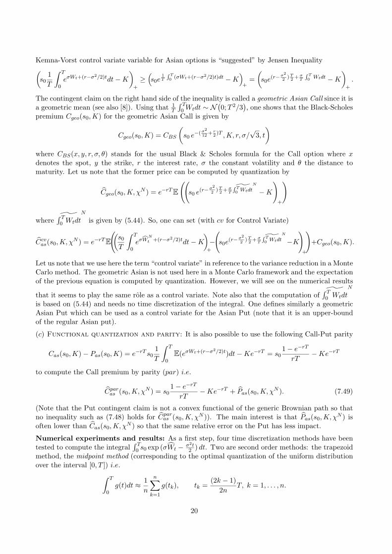
Table 1 below provides the first three quantities for some values of N , namely N = 1, 10,100, 1 000, 10 000 and 11 519 (the full record table, the record quantizer list including the distributionsare available at the same URL up to 11 519). Figures 1, 2, 3 show the scaled product quantizers ofthe Brownian motion on [0, 1] for N = 10, 48 and for the “record value” of N = 100 that is Nrec = 96.

N Nrec Quant. Error Opti. Decomp.1 1 0.7071 110 10 0.3138 5 – 2100 96 0.2264 12 – 4 – 2

1 000 966 0.1881 23 – 7 – 3 – 210 000 9 984 0.1626 26 – 8 – 4 – 3 – 2 – 211 519 11 232 0.1617 26 – 9 – 4 – 3 – 2 – 2

Table 1 Brownian motion: Some typical “record” values for numerical implementations

Fig.2 shows the graphs of both N 7→ DWNrec

(√λ ⊗ xNrec) and N 7→ DW

N (√λ ⊗ xopt) for N ∈

1, . . . , 1 000. Fig.3 depicts log(N) 7→ (DWNrec

(√λ ⊗ xNrec))

−1 which emphasizes logN behaviour ofthe distortion. The coefficients obtained by linear regression yield

1

DWNrec

(√λ⊗ xNrec)

≈ 4 logN + 2 i.e. DWNrec

(√λ⊗ xNrec) ≈

0.25logN + 0.5

, 1 ≤ N ≤ 10 000.

The lower and upper bounds provided by (2.1) and (5.29) respectively are on [0, 1],

1π2

22

22−1(2− 1)=

2π2≈ 0.2026 < 0.25 < 1.2040 ≈ 1

π2(1 + 2π

√3). (5.41)

15

This points out that optimal scalar quantizers are nearly globally optimal for Brownian Motion (atleast within this range of values for N). For higher values of N one may give up the blind optimizationprocedure and rely on the asymptotic optimal sizes given by (5.27). Proposition 3 that is

One may even speed up this approach by using the asymptotic estimate mN ∼ log(N) for largevalues of N (since b = 2 for the Brownian Motion). One may note that in fact

N` ≈√

λ`λ`N

, ` = 1, . . . ,mN .

In practice, the product N ′ = N1 × · · · × N`N can be significantly lower than N , especially when Nis not too large, owing to the truncation effect. So a more efficient choice is to consider the uppertruncation instead of the regular integral value in (5.27) although this time N ′ can be . . . significantlylarger than N . Furthermore, note that N ′ is a priori not a record integer Nrec and that this verydecomposition can be sub-optimal for N ′. Table 2 below gives some examples of such decompositionscorresponding to values of N beyond the shortcoming of the optimization procedure at Nmax = 11 519:thus N = 13 500 in Table 2 provides worse results than N = 11 232 in Table 1.

N Quant. Error Decomp13 500 0.16217 25 – 9 – 5 – 340 500 0.15362 25 – 9 – 5 – 4 – 3 – 3104 400 0.14811 29 – 10 – 6 – 5 – 4 – 3313 200 0.14140 29 – 10 – 6 – 5 – 4 – 3 – 3

Table 2. Brownian motion: some decompositions for higher values of N

5.4.2 Application to computable rate optimal quantizers for the antiderivative of theBrownian motion

We will illustrate in this short paragraph how rate optimal product quantizers of the Brownian motioncan produce some (non Voronoi) rate optimal quantizers of its antiderivative. This process is involvedin the control variate variable of the Asian Call (see paragraph 7.1).

First note that one can integrate a Karhunen-Loeve expansion of the Brownian motion. In fact,h 7→ ∫ .

0 h(s)ds being a Lipschitz continuous function from L2T

into (C([0, T ]), ‖ . ‖sup), one has, inL2

(C([0,T ]),‖.‖sup)(P) (and P-a.s. in L2T

):

∫ t

0Wsds

L2T=

∑

`≥1

λ` ξ`

√2T

(1− cos

(t√λ`

))with λ` :=

(T

π(`− 1/2)

)2

, ` ≥ 1, (5.42)

= 2

√2T

∑

`≥1

λ` ξ` sin2

(t

2√λ`

)(5.43)

where: – (ξ`)`≥1 is i.i.d., normally distributed (and comes from the Karhunen-Loeve extension of W ),

– the sequence(t 7→

√2T

(1− cos

(t√λ`

)))`≥1

is not orthonormal in L2T

.

In fact, the expansion (5.42) converges P-a.s. and in L1(P), uniformly in t∈ [0, T ], since

supt∈[0,T ]

∣∣∣∣∣∣∑

`≥1

λ` ξ` sin2

(t

2√λ`

)∣∣∣∣∣∣≤

∑

`≥1

λ`|ξ`|.

16

The series on the right hand of the inequality lies in L1(P) since∑

`≥1 λ` < +∞ and ξ` ∼ ξ1∈ L1(P).The same holds for the integrated product quantizer expansion, that is

∫ .

0Wsds :=

∫ .

0W√λ⊗x

s ds = 2

√2T

∑

`≥1

λ` ξ` sin2

(t

2√λ`

)(5.44)

since, by stationarity of the quantizer x(`) of ξ`, E|ξ`| ≤ E|ξ`| for every ` ≥ 1 (note that the P-a.s.

convergence is trivial since ξ = 0 for ` large enough). One has to be aware that ˜∫ .0 Wsds is neither

a product nor a Voronoi quantization since it is defined on the Voronoi tessellation of the Brownianmotion. For this very reason it is easy to compute and furthermore it satisfies a kind of stationary

equation: one checks that σ( ˜∫ .

0 Wsds) = σ(W ) = σ(ξ`, ` ≥ 1) so that, h 7→ ∫ .0 h(s)ds being continuous

and linear on L2T

,

E(∫ .

0Wsds |

∫ .

0Wsds

)= E

(∫ .

0Wsds | W

)=

∫ .

0Wsds.

Proposition 5 Let xN ∈ Opq(N), N ≥ 1. Set ˜∫ .0Wsds

N

:= ˜∫ .0Wsds

√λ⊗xN

.(a) The quadratic quantization error is given by

∥∥∥∥∥∥

∫ .

0Wsds−

∫ .

0Wsds

N∥∥∥∥∥∥

2

2

= 3∑

`≥1

λ2`

(1− (−1)`−1 4

√λ`

3T

)minRN`

DN (0;1)N`

. (5.45)

If (√λ⊗ xN )N≥1 is rate optimal for W then it is rate optimal for its antiderivative in the sense that

∥∥∥∥∥∥

∫ .

0Wsds−

˜∫ .

0Wsds

N∥∥∥∥∥∥

2

2

= O((logN)−32 ).

(b) The L1(P)-mean ‖ . ‖sup-quantization error satisfies

E

supt∈[0,T ]

∣∣∣∣∣∣

∫ t

0Wsds−

˜∫ t

0Wsds

N∣∣∣∣∣∣

≤ 2

√2T

∑

`≥1

λ` minRN`

√DN (0;1)N`

. (5.46)

Proof: (a) Temporarily set E`(t) = 1− cos(

t√λ`

). Then |E`|2

L2T

= T(

32 − 2(−1)`−1

√λ`T

)

and

∣∣∣∣∣∣

∫ .

0Wsds−

∫ .

0Wsds

N∣∣∣∣∣∣

2

L2T

=2T

∑

`,m≥1

λ`λmE(ξ` − ξ`)(ξm − ξm) (E` |Em)L2T

so that

∥∥∥∥∥∥

∫ .

0Wsds−

∫ .

0Wsds

N∥∥∥∥∥∥

2

2

=2T

∑

`≥1

λ2` E(ξ` − ξ`)2|E`|2

L2T

.

This follows from the fact that the random variables ξ`− ξ`, ` ≥ 1, are independent and centered sinceE(ξ` − ξ`) = E(E(ξ`|ξ`) − ξ`) = 0. The rate of decay follows from the optimal size allocation in theright hand side of Inequality (5.46) which is standard (see [11]).

17

(b) easily follows from

supt∈[0,T ]

∣∣∣∣∣∣

∫ t

0Wsds−

˜∫ t

0Wsds

N∣∣∣∣∣∣

= 2

√2T

supt∈[0,T ]

∣∣∣∣∣∣∑

`≥1

λ`(ξ` − ξ`) sin2

(t

2√λ`

)∣∣∣∣∣∣≤ 2

√2T

∑

`≥1

λ` |ξ` − ξ`|. ♦

Remarks. • One derives similarly from item (b) that the lowest L1(P)-mean L∞(dt)-quantizationerror goes to zero at a O

((log(N))−1

)-rate.

• Some rates can be obtained for higher iterated integrals (and the Brownian bridge too).

6 The Romberg log-extrapolation

The aim of this paragraph is to propose a Romberg like extrapolation method to speed up the con-vergence of the quantization method. What follows is partially heuristic in that it relies on someclaims on functional quantization which are still conjectures. For these reasons, we will focus on theBrownian motion and will not look for optimal assumptions.

Let Ψ : (L2T, | . |

L2T

) → R be a three times differentiable functional such that D2Ψ and D3Ψ are

bounded. Let (χN )N≥1 denote a sequence of stationary rate optimal quantizers of the Brownianmotion W (e.g. χN =

√λ⊗ xNopt in the K-L basis) and let WN denote their related quantizations.

It follows from the Taylor formula and Proposition 4 (stationarity property of WN ) that one caneasily find ζ ∈ L2

Tsuch that

E(Ψ(W )) = E(Ψ(WN )) +12E(D2Ψ(WN ).(W − WN )⊗2) +

16E(D3Ψ(ζ).(W − WN )⊗3)

since E(DΨ(WN ).(W −WN )) = E(DΨ(WN ).(W −E(W | WN ))) = 0. Then, D2Ψ being bounded andχN -rate optimal,

E(D2Ψ(WN ).(W − WN )⊗2) = O((logN)−1

),

but recent (finite dimensional) results (see [1], Theorem 6) suggest that, more precisely,

E(D2Ψ(WN ).(W − WN )⊗2) = 2κ(logN)−1 + o((logN)−1) as N →∞

where κ>0 is real constant. Moreover, still relying on [1] (Proposition 1), one shows that

E|W − WN |3L2T

= O((logN)−32

+η), ∀ η > 0.

Then, a Romberg like speeding up procedure can be implemented as follows: one computes E(Ψ(WM ))and E(Ψ(WN )), M < N , M ³ N r, r∈ (0, 1). Solving the linear system

E(Ψ(W )) = E(Ψ(WM))+κ

logM+O((logM)−

32

+η), E(Ψ(W )) = E(Ψ(WN))+κ

logN+O((logN)−

32

+η)

yields the announced log-extrapolation formula

E(Ψ(W )) =logN×E(Ψ(WN ))− logM×E(Ψ(WM ))

logN − logM+O

((logN)−

32

+η), ∀ η > 0. (6.47)

So we passed from a O((logN)−1)-rate to an (at least) O(

(logN)−32

+η)

-rate.

18

7 Pricing derivatives using functional quantization

7.1 Pricing Asian options in a Black-Scholes model

One considers a Black-Scholes dynamics with maturity T ,

dSt = St (rdt+ σ dWt), S0 = s0 > 0 (r > 0).

The premium of an Asian (European) Call option with strike price K is given by

Cas(s0,K) := e−rTE((

1T

∫ T

0Stdt−K

)

+

)= e−rTE

((s0

1T

∫ T

0eσWt+(r−σ2/2)tdt−K

)

+

)

where x := max(x, 0) denotes the nonnegative part of the real number x. We want to approximateCas(s0,K) using quadratic functional quantization.

(a) “Crude” functional quantization method: One simply computes

Cas(s0,K, χN ) := e−rTE

((s0

1T

∫ T

0eσ

cWNt +(r−σ2/2)tdt−K

)

+

)

where the process (WN

t )t∈[0,T ] denotes the quantization of the Brownian motion W by the productquantizer χN :=

√λ ⊗ xNrec which induces the lowest quantization error among all (Karhunen-Loeve)

product quantizers having at most N -components. The functional

ω 7→(s0

T

∫ T

0eσω(t)+(r−σ2/2)tdt−K

)

+

is convex, consequently combining (4.16) and the stationarity of (Wt)t∈[0,T ]

Cas(s0,K, χN ) ≤ Cas(s0,K). (7.48)

This bound can be improved by considering any√λ-scaled product quantizer

√λ ⊗ x of W , with

x∈ Opq(N). Then, with obvious notations

supx∈Opq(N)

Cas(s0,K,√λ⊗x) ≤ Cas(s0,K).

Furthermore, it follows from (4.13) and (4.18) that, for any x∈ Opq(N),

0 ≤ Cas(s0,K)− Cas(s0,K,√λ⊗x) ≤ 2 s0σe

−rT+(r−σ2

2)+T E(| exp (σW )|

L2T

) ‖W − W√λ⊗x‖2

≤ 2 s0e−(r∧σ2

2)T (eσ

2T − 1)12 ‖W − W

√λ⊗x‖2 .

In particular

0 ≤ Cas(s0,K)− Cas(s0,K, χN ) ≤ 2 s0e

−(r∧σ2

2)T (eσ

2T − 1)12 minx∈Opq(N)

‖W − W√λ⊗x‖2 = O((logN)−

12 )

as N →∞. One also has, using (4.17), that

|E SχNT− EST | = o((logN)−

1−ε2 ) as N → +∞ for every ε > 0.

(b) Functional quantization and geometric control variate variable: The standard

19

Kemna-Vorst control variate variable for Asian options is “suggested” by Jensen Inequality(s0

1T

∫ T

0eσWt+(r−σ2/2)tdt−K

)

+

≥(s0e

1T

R T0 (σWt+(r−σ2/2)t)dt −K

)+

=(s0e

(r−σ2

2)T

2+ σT

R T0 Wtdt −K

)

+

.

The contingent claim on the right hand side of the inequality is called a geometric Asian Call since it isa geometric mean (see also [8]). Using that 1

T

∫ T0 Wtdt ∼ N

(0;T 2/3

), one shows that the Black-Scholes

premium Cgeo(s0,K) for the geometric Asian Call is given by

Cgeo(s0,K) = CBS

(s0 e−(σ

2

12+ r

2)T ,K, r, σ/

√3, t

)

where CBS(x, y, r, σ, θ) stands for the usual Black & Scholes formula for the Call option where xdenotes the spot, y the strike, r the interest rate, σ the constant volatility and θ the distance tomaturity. Let us note that the former price can be computed by quantization by

Cgeo(s0,K, χN ) = e−rTE

((s0 e

(r−σ2

2)T

2+ σT

˜R T0 Wtdt

N

−K)

+

)

where ˜∫ T0 Wtdt

N

is given by (5.44). So, one can set (with cv for Control Variate)

Ccvas(s0,K, χN ) = e−rTE

((s0

T

∫ T

0eσ

cWN

t +(r−σ2/2)tdt−K)

+

−(s0e

(r−σ2

2)T

2+ σT

˜R T0 Wtdt

N

−K)

+

)+Cgeo(s0,K).

Let us note that we use here the term “control variate” in reference to the variance reduction in a MonteCarlo method. The geometric Asian is not used here in a Monte Carlo framework and the expectationof the previous equation is computed by quantization. However, we will see on the numerical results

that it seems to play the same role as a control variate. Note also that the computation of ˜∫ T0 Wtdt

N

is based on (5.44) and needs no time discretization of the integral. One defines similarly a geometricAsian Put which can be used as a control variate for the Asian Put (note that it is an upper-boundof the regular Asian put).

(c) Functional quantization and parity: It is also possible to use the following Call-Put parity

Cas(s0,K)− Pas(s0,K) = e−rT s01T

∫ T

0E(eσWt+(r−σ2/2)t)dt−Ke−rT = s0

1− e−rTrT

−Ke−rT

to compute the Call premium by parity (par) i.e.

Cparas (s0,K, χN ) = s0

1− e−rTrT

−Ke−rT + Pas(s0,K, χN ). (7.49)

(Note that the Put contingent claim is not a convex functional of the generic Brownian path so thatno inequality such as (7.48) holds for Cparas (s0,K, χ

N )). The main interest is that Pas(s0,K, χN ) is

often lower than Cas(s0,K, χN ) so that the same relative error on the Put has less impact.

Numerical experiments and results: As a first step, four time discretization methods have beentested to compute the integral

∫ T0 s0 exp (σWt − σ2t

2 ) dt. Two are second order methods: the trapezoidmethod, the midpoint method (corresponding to the optimal quantization of the uniform distributionover the interval [0, T ]) i.e.

∫ T

0g(t)dt ≈ 1

n

n∑

k=1

g(tk), tk =(2k − 1)

2nT, k = 1, . . . , n.

20

and two are fourth order methods: the fourth-order Runge-Kuta method and the fourth order midpointmethod, based on the introduction of the (weighted) derivatives of g at points tk.

We specified numerical values for the parameters following the tests carried out in [10], i.e.

s0 = K = 100, T = 1, r = 10%, σ = 20%.

The reference values for the Asian Call and Put are, still following [10]

Asian Call Premium = 7.041 Theoretical Asian Put Premium = 2.362

The best compromise between complexity and efficiency is the second order midpoint method (seeFigure 4). To reach this conclusion we let n become large for two values of N (using the crudefunctional quantization method (FQ) for the Asian Call). Let us note that the “limiting value” (whenthe time discretization step 1/n goes to 0) looks far the true value (≈ 7.041) with all the four methods.This comes from the scale specification since our aim in this first experiment is exclusively to comparethe different time integration methods. In fact, it will be seen below that, for a given couple (n,N) oftime-space discretization parameters, best prices are usually obtained using the Call-Put parity.

Now, we come to testing the FQ method itself. Asian option premia are computed using N = 96(Table 3), N = 966 (Table 4) and N = 9 984 (Table 5). Time integration is performed by the midpointscheme with n = 20. For each values of N , the second row displays 2× StdN where StdN denotes therelative standard deviation of the corresponding Monte Carlo N -estimator which defines its 95.5%-confidence interval. This estimator is based on the simulation of the K-L expansion (5.36) of theBrownian motion (truncated at ` = 100). The third row shows the decomposition producing thelowest distortion and its value. Then, the successive rows give the results for different factorizationsof N . The third (resp. fourth) column gives the Call premium Cas by “crude” FQ (resp. Ccvas withthe Kemna-Vorst control variate). The fifth (resp. sixth) one displays the Put premium Pas obtainedby “crude” FQ (resp. P cvas with the control variate). The seventh (resp. eighth) one displays the Callpremium obtained using the Call-Put parity relation (7.49) and the fifth column (resp. using (7.49)and the sixth column).

The results in Tables 3, 4, 5 are in a descending order with respect to the Call premia obtained bycrude FQ (column 3). This is justified by the fact that this method always produces a lower boundfor the premium (although this sorting is unrealistic in practice).

For both the decomposition with the lowest distortion (?) – the one of interest for applications –and the one with the highest premium Cas for the Call (fourth row of every table), the relative erroris added between brackets.

At this stage, the tables suggest that the most performing method to compute the Call (at-the-money) is the computation by parity, from the Put computed by “crude” FQ using the “record” scaledproduct quantizer χN (decomposition ?, see column 7 in Tables 3, 4, 5): the relative error is alwaysless than 0.2% (but one loses the lower bound property). as N ≥ 1 000. Within this range of values ofN (N ≤ 10 000) the computation is instantaneous. Let us note that the Kemna-Vorst control variatevariable (columns 4, 6, 8) seems globally less efficient than in the Monte Carlo method but give errorswhich are of the same order than the relative standart deviations of the Monte-Carlo estimators basedon K-L expansion (second line) at least for N = 96 and N = 966. This tell us that this control variatevariable seems to play the same role both in the functional quantization and Monte Carlo methodwhen N is small. When N becomes larger, this control variate method seems more efficient in theMonte Carlo method (based on the K-L expansion (5.36)).

21

N = 96 n bCas bCcvas bPas bP cvas bCparasbCpar&cvas Decomposition

2× Std96 20 (24.49%) (1.14%) (37.11%) (1.33%) (12.45%) (0.47%) -

96 20 Best decomp(?): 96 = 12 × 4× 2, Distor? = 0.051276

96 20 6.957 6.971 2.387 2.396 7.066 7.075 24 – 4(1.2%) (1.0%) (1.1%) (1.4%) (0.3%) (0.5%)

96 20 6.957 6.981 2.377 2.393 7.056 7.071 16 – 3 – 296 20 6.953 6.983 2.372 2.390 7.051 7.069 12 – 4 – 2 ?

(1.3%) (0.8%) (0.4%) (1.2%) (0.1%) (0.4%)96 20 6.952 6.969 2.386 2.399 7.0651 7.078 32 – 396 20 6.951 6.975 2.379 2.396 7.0582 7.074 16 – 696 20 6.950 6.972 2.381 2.396 7.0595 7.075 24 – 2 – 296 · · · · · · · · · etc · · · · · · · · · · · ·

Table 3. Asian Call approximations for N = 96

N = 966 n bCas bCcvas bPas bP cvas bCparasbCpar&cvas Decomposition

2× Std966 20 (7.72%) (0.36%) (11.70%) (0.42%) (3.93%) (0.14%) -

966 20 Best decomp(?): 966 = 23 × 7 × 3 × 2, Distor? = 0.035195

966 20 6.988 6.999 2.377 2.383 7.055 7.062 23 – 7 – 3 – 2 ?(0.7%) (0.5%) (0.3%) (0.3%) (0.2%) (0.3%)

966 20 6.987 6.992 2.382 2.386 7.061 7.065 46 – 7 – 3966 20 6.984 6.995 2.378 2.385 7.057 7.064 23 – 7 – 6966 20 6.984 6.989 2.384 2.388 7.063 7.067 69 – 7 – 2966 20 6.983 6.994 2.379 2.386 7.058 7.065 23 – 14 – 3966 20 6.980 6.990 2.380 2.387 7.059 7.066 23 – 21 – 2966 20 6.971 6.977 2.388 2.393 7.067 7.072 69 – 14966 20 6.970 6.978 2.388 2.393 7.066 7.072 46 – 21966 20 6.970 6.978 2.387 2.393 7.066 7.072 42 – 23

Table 4. Asian Call approximations for N = 966

N n bCas bCcvas bPas bP cvas bCparasbCpar&cvas Decomposition

2× Std9984 20 (2.40%) (0.11%) (3.64%) (0.13%) (1.22%) (0.04%) -

9 984 20 Best decomp.(?): 9 984 = 26×8×4×3×2×2, Distor? = 0.026435

9 984 20 7.004 7.007 2.377 2.380 7.056 7.058 52 – 8 – 4 – 3 – 2(0.5%) (0.4%) (0.6%) (0.7%) (0.2%) (0.2%)

9 984 20 7.003 7.008 2.376 2.379 7.055 7.058 39 – 8 – 4 – 2 – 2 – 29 984 20 7.003 7.008 2.376 2.379 7.055 7.058 39 – 8 – 4 – 4 – 29 984 20 7.003 7.006 2.378 2.380 7.057 7.059 52 – 12 – 4 – 2 – 29 984 20 7.003 7.007 2.377 2.380 7.056 7.059 52 – 8 – 6 – 2 – 29 984 20 7.003 7.006 2.378 2.380 7.056 7.059 48 – 13 – 4 – 2 – 29 984 · · · · · · · · · etc · · · · · · · · · · · ·9 984 20 7.002 7.005 2.378 2.380 7.057 7.059 52 – 16 – 3 – 2 – 29 984 20 7.002 7.010 2.373 2.378 7.052 7.057 26 – 8 – 4 – 3 – 2 – 2 ?

(0.5%) (0.5%) (0.4%) (0.3%) (0.1%) (0.3%)9 984 · · · · · · · · · etc · · · · · · · · · · · ·

Table 5. Asian Call approximations for N = 9 984

Further values reported in Table 6 below were obtained using the N` given by (5.27) (in fact theirupper truncation) so they are a priori not even optimal among all the decompositions of their productN = N1 · · ·Nm

N. This confirms that the convergence as N grows is slow. The quite good results

22

N n bCas bCcvas bPas bP cvas bCparasbCpar&cvas Decomposition

13 500 20 7.002 7.010 2.373 2.378 7.052 7.057 25 – 9 – 5 – 4 – 3(0.5%) (0.4%) (0.5%) (0.7%) (0.06%) (0.2%)

40 500 20 7.005 7.013 2.372 2.377 7.050 7.055 25 – 9 – 5 – 4 – 3 – 3(0.5%) (0.4%) (0.5%) (0.7%) (0.03%) (0.2%)

104 400 20 7.009 7.015 2.372 2.376 7.051 7.055 29 – 10 – 6 – 5 – 4 – 3(0.5%) (0.4%) (0.5%) (0.7%) (0.04%) (0.2%)

313 200 20 7.012 7.018 2.371 2.375 7.050 7.054 29 – 10 – 6 – 5 – 4 – 3 – 3(0.4%) (0.3%) (0.4%) (0.5%) (0.03%) (0.2%)

Table 6. Asian Call approximations for larger values of N

obtained for small values of N is an important asset of functional quantization.The Romberg log-extrapolation. Although the regularity assumptions are clearly not fulfilledby the Asian payoff, we tested the Romberg log-extrapolation (6.47) and reported in Table 7 belowthe results obtained with N = 966 and M = 9 984 by using the record product quantizers. It turnsout that this drastically improves all the approaches in such a way which seems not to depend on theapproach itself (“crude” Functional Quantization, control variate variable, by parity, and so on). Thissuggests that a functional quantization approach including a Romberg log-extrapolation provides anextremently efficient numerical method for this problem.

Romberg[966-9984] n bCas bCcvas bPas bP cvas bCparasbCpar&cvas

20 7.041 7.041 2.364 2.364 7.042 7.042(0.00%) (0.00%) (0.08%) (0.08%) (0.01%) (0.01%)

Table 7. Romberg[966-9984] log-extrapolation using record product quantizers

7.2 Pricing vanilla options in a Heston model

In this paragraph, we consider a Heston stochastic volatility model for the dynamics of an asset priceprocess:

dSt = St(r dt+√vt)dW 1

t , S0 = s0 > 0, (7.50)

dvt = k(a− vt)dt+ ϑ√vtdW

2t v0 > 0, with <W 1,W 2>t= ρ t, ρ∈ [−1, 1],

where r denotes the (constant) interest rate and (vt) denotes the square stochastic volatility processand a, k, ϑ are non-negative real parameters. This model was introduced by Heston in 1993 (see [6]).The equation for the (vt) has a unique (strong) pathwise continuous solution living in R+ (see e.g. [9]and [7], p.235). Thereis a semi-closed form for vanilla European Call and Put options based on someintegrals of the characteristic function for which a closed form is available (see [9]). We will use it asa reference for our experiments. Our aim is to price by functional quantization (at time 0) EuropeanCalls (and Puts) on the underlying asset (St) with strike price K and maturity T > 0, i.e.

CallHest(S0,K, r) = e−rTE((ST −K)+) and PutHest(S0,K, r) = e−rTE((K − ST )+).

As a first step, we follow an approach which works for more general dynamics of the stochasticvolatility. First we project W 1 onto W 2 so that

W 1t = ρW 2

t +√

1− ρ2 W 1t ,

with W 1 a standard Brownian motion independent of W 2. Ito calculus shows that

St = s0 exp(−ρ

2

2vt t+ ρ

∫ t

0

√vsdW

2s

)exp

((r − 1− ρ2

2vt)t+

√1− ρ2

∫ t

0

√vsdW

1s

)

23

with vt = 1t

∫ t0vsds. Consequently, using the independence of W 1 and W 2, one derives that

CallHest(S0,K, T, v0, r) = E(e−rTE

((ST −K)+ | FW 2

T

))= E

(CallBS

(S

(v)0 ,K, T,

((1− ρ2)vT

) 12 , r

))

with S(v)0 = s0 exp

(−ρ

2

2vT T + ρ

∫ T

0

√vsdW

2s

)

where CallBS(s0,K, T, σ, r) denotes the regular (r, σ, T )-Black-Scholes model premium function. Thenthe specific dynamics of (vt) yields(1)

∫ t

0

√vsdW

2s =

vt − v0 − kat+ k∫ t

0 vsds

ϑ

so that finally

CallHest(S0,K, T, v0, r) = EΦc(ρ(vT − v0), vT ) (7.51)

with Φc(v, v) = CallBS

(s0 exp

(−ρ

(ka

ϑ− (

k

ϑ− ρ

2)v

)T +

v

ϑ

),K, T,

((1− ρ2)v

) 12 , r

).

An analogous formula holds for PutHest(S0,K, T, v0, r) by replacing mutatis mutandis CallBS by PutBSin (7.51). Note that when ρ = 0, (7.51) only depends on the L2-continuous linear functional vT .

7.2.1 The quantization procedure

A first way to numerically quantize (vt) is to follow – at least formally – the approach developedin [13] to quantize Brownian diffusions with Lipschitz continuous coefficients. One considers again thesequence χN :=

√λ ⊗ xNrec, N ≥ 1, of record product quantizers of the standard Brownian motion

(which are explicit C∞ functions). For convenience, we will consider now the “record” subsequencei.e. assume that N=Nrec.

Assume for a while that (vt) is a generic Brownian diffusion

dvt = b(vt)dt+ ϑ(vt)dW 2t (ϑ ≥ 0)

Some quantizers for (vt) can be designed from the sequence (χN ) as follows: one introduces theLamperti transform of the diffusion defined by L(v) :=

∫ v0

dvϑ(v) (assumed to be real-valued and in-

creasing). Then, Ut := L(vt) satisfies is solution of the SDE

dUt = β(Ut)dt+ dWt

with a linear Brownian perturbation term. Then, one defines, a N -quantizer of (vt) by setting

yNi (t) = L−1(uNi (t)) where uNi (t) = L(v0) +∫ t

0β(uNi (t))dt+ χNi (t), i = 1, . . . , N.

Elementary computations show that yN = (yNi )1≤i≤N is solution of the system of integral equations

yNi (t) = v0 +∫ t

0[b(yNi (s))− 1

2ϑϑ′(yNi (s))]ds+

∫ t

0ϑ(yNi (s))dχNi (s), i = 1, . . . , N. (7.52)

1The key point in what follows is to express the stochastic integralR t

0

√vsdW

2s as a functional of vt, v0 and an integral

functional of (vs). If the variance process follows a general diffusion process dvt = b(vt)dt + ϑ(vt)dW2t then one may

apply under appropriate regularity assumption, Ito’s formula to the function ϕ(v) :=√v/ϑ(v) to get such an expression.

24

When b and ϑ are Lipschitz continuous, it is established in [13] (Theorem 1 and the following Ap-plication) that if the sequence (χN )N≥1 is rate optimal in L2

L2T

(Ω,P) for the Wiener measure, then

(yN )N≥1 is rate optimal in LpL2T

(Ω,P) for every p∈ [1, 2). More precisely, it is established in [13] that

the sequence of non-Voronoi N -quantizations

vNt =∑

1≤i≤NyNi (t)1Ci(χN )(W

2), N ≥ 1,

satisfies ‖ |v − vN |L2T

‖p = O((logN)−1/2), p∈ [1, 2). When p = 2 a straightforward adaptation of the

proof yields a O((logN)−12

+ε)-rate in LpL2T

(Ω,P) for every ε > 0. The quantization vNt is not Voronoi

since it is defined on the Voronoi tessellation of W 2, but its distribution is given by the PW -weightsof the cells Ci(χN ) which are known by (5.38). In our non-Lipschitz setting (b(v) = −k(v − a),ϑ(v) = ϑ

√v), yN satisfies

yNi (t) = v0 + k

∫ t

0

(a− ϑ2

4k− yNi (s)

)ds+ ϑ

∫ t

0

√yNi (s)dχNi (s), i = 1, . . . , N. (7.53)

If a > ϑ2/(4k), any solution of (7.53) is positive and, once again a simple adaptation of the proof ofTheorem 1 in [13] shows that ‖ |v − vN |

L2T

‖2 = O((logN)−12

+ε). Numerical implementation of this

functional quantization method simply needs to use a discretization scheme of (7.53) like the Euler,the midpoint or the Runge-Kuta schemes.

However, in view of investigating the efficiency of functional quantization, this approach suffersfrom mixing two kinds of error: one due to the discretization scheme of the integral equation systemand one due to functional quantization. So, to be more illustrative of the numerical performances offunctional quantization, we will consider the Heston model in the case a = ϑ2

4k since, as noticed byRogers in [19], one may assume without loss of generality that the process (vt) is the square of a scalarOrnstein-Uhlenbeck process

dXt = −k2Xtdt+

ϑ

2dW 2

t , X0 =√v0. (7.54)

Having in mind that the N -quantizers χN given by (5.37) read

χNi (t) =

√2T

∑

`≥1

x(N`)i`

T

π(`− 1/2)sin

(π(`− 1/2)

t

T

), i = (i1, . . . , i`, . . .)∈

∏

`≥1

1, . . . , N`,

where x =∏`≥1 x

(`)∈ Opq the solutions of the integral system (7.52) associated to X

xi(t) =√v0 − k

2

∫ t

0xi(s) ds+

ϑ

2χNi (t), i = 1, . . . , N (7.55)

are given for every i = (i1, . . . , i`, . . .)∈∏`≥11, . . . , N` by

xNi (t) = e−kt/2√v0 +

ϑ

2

∑

`≥1

x(`)i`c` ϕ`(t) with c` :=

T 2

(π(`− 1/2))2 + (kT/2)2

and ϕ`(t) :=

√2T

(π

T(`− 1/2) sin

(π(`− 1/2)

t

T

)+k

2

(cos

(π(`− 1/2)

t

T

)− e−kt/2

)).

This time, still following [13], we have for every p∈ [1, 2),

‖XN −X‖p ≤ Cp,k,ϑ,T ‖W 2χN −W 2‖2 = O

((logN)−

12

)(7.56)

25

where XN is the non-Voronoi quantization defined by

XNt =

N∑

i=1

xNi (t)1Ci(χN )(W2) = e−kt/2

√v0 +

ϑ

2

∑

`≥1

ξx(`)

` c` ϕ`(t), t∈ [0, T ].

One designs a (non-Voronoi) N -quantization for the process (vt) by setting

vNt = (XNt )2 =

∑

i

(xNi (t))21Ci(χN )(W2). (7.57)

Then, one derives from (7.56) that, for every p∈ [1, 2],

‖ |vN − v|L2T

‖p = O(

(logN)−( 12−ε)

)for every ε > 0. (7.58)

Finally, in practice, one computes CallHest(S0,K, T, r) by

CallHest(s0,K, T, v0, r) = E(Φc(ρ(vT − v0), vT )) (7.59)

≈ E(Φc(ρ(vT − v0), vT ))

=∑

i

Φc

(ρ

((xNi )2(T )− v0

), (xNi )2(T )

)P(W 2 = χNi ) (7.60)

where the probability distribution (P(W 2 = χNi ))i is given by (5.38). When ρ 6= 0, no simple errorbound is available since we do not know the rate of pointwise quantization of vT by quadratic functionalquantizers.

When ρ = 0, v 7→ Φc(0, v0, v) is clearly Lipschitz, so a O(

(logN)−( 12−ε)

)-rate holds in (7.60).

Furthermore, functions σ 7→ PutBS(s0,K, T, σ, r) and its Call counterpart are infinitely differentiableon (0,+∞) and u 7→ uT := 1

T

∫ T0 u(s)ds is an L2

T-continuous linear functional. On the other hand,

the solution of the integral equation x(t) = x(0)− k2

∫ t0 x(s)ds+ ϑ

2 ξ(t) is also an L2T

-continuous linearfunctional functional of ξ. Consequently, one may write (7.59)

PutHest(s0,K, T, r) = E(Ψp(W 2)) and CallHest(s0,K, T, r) = E(Ψc(W 2))

where Ψp and Ψc are infinitely differentiable and Ψp is bounded with all its differentials .

7.2.2 Numerical experiments and results

All the formulæ for the Call can be straightforwardly adapted to the Put. Furthermore, the Call-Putparity holds which is a second way to compute the Call premium which has a lower variance. We usedas a reference price the closed form available for the Heston model (approximate accuracy 10−2).

Following the results of the experiments carried out with the Asian option we compute timeintegrals by the midpoint method with n = 20, i.e.

(xNi )2 =1T

∫ T

0(xNi (s))2ds ≈ 1

n

n∑

k=1

(xNi (tk))2 with tk =(2k − 1)T

2n.

with the lowest quadratic quantization error as theywere computed The parameters of the Hestonmodel are specified as follows

s0 = 50, r = 0.05, T = 1, ρ = 0.5, v0 = a = 0.01, ϑ = 0.1, k = 0.25

26

so that ϑ2 = 4 k a (and E vt = a, t∈ [0, T ]). In this section, we carried out our numerical experiments ona whole vector of strike prices, K running from 44 up to 56 (with step 1) to evaluate the performancesof the method for in-the-money, at-the-money and out-of-the-money options. The premia of theseHeston Call options were computed using:

– formula (7.51) (“crude” FQ integration),– the Call-Put parity equation combined with Formula (7.51) for Put options.

We implemented (using MATLAB on a G4 (800 Mhz) Apple computer):– five sizes of N -quantizations of (vt), computed by (7.57) from optimal scaled product quantizers

of the Brownian Motion, namely N = 96, 966, 9 984 (which are “record values”), 40 500, 104 400(which are “close” to “record values”). Note that we no longer tried optimizing over Opq(N) as wedid for Asian Call.

– one Romberg log-extrapolation from the results obtained with N = 966 and M = 9984. Notethat we do not provide theoretical justification for this Romberg extrapolation when ρ 6= 0 so this isjust a numerical experiment.

– a “crude” Monte Carlo N -estimator

CallMCHest(s0,K, T, r) :=

1N

∑

1≤i≤NΨc(W 500,(i))

where W 500,(i) are N independent copies of the K-L expansion of the Brownian motion (truncated at` = 500). (Its relative Standard Deviation StdN is estimated from that of Ψc(W 500,(1))).

The results are reported in Figures 5, 6, 8 and in Table 7. In the first two figures are depictedthe absolute and relative errors obtained when pricing Heston Calls by functional quantization (FQ)either directly (in Figure 5) or through the Call-Put parity equation (in Figure 6). First we do observea convergence behaviour as N grows. This convergence is slow as expected when N grows but fast forsmall values of N , so that with N ≈ 10 000, the resulting error is less than 4 cents by the “crude” FQmethod and less than 2 cents by the parity-FQ method. Higher values of N seems of little numericalinterest, given that the computational complexity grows linearly with N .

As concerns the comparison with the “crude” Monte Carlo method, we reported in Table 8 below(third row) 2×StdN , where StdN denotes the (relative) standard deviation of the above MC estimator(for N = 10 000). This quantity defines its 95.5%-confidence interval. One verifies that 2× Std10 000

is slightly higher (say 10 to 30%) than the relative error induced by “crude” FQ-integration withN = 9984 (fourth row). When N = 966 for “crude” FQ and a 1 000-Monte Carlo estimator therelative error of the pure FQ is this time lower than Std1 000 itself (these results are not reproducedhere). A similar phenomenon occurs when using the C-P parity approach (not reproduced here) atmuch lower error level (row 5). In all cases, the relative error increases when the strike price K of theCall goes deeper out-of-the-money (although the absolute error is in fact decreasing).

In fact, the most striking fact provided by these experiments is the confirmation of the outstandingperformances of the “Romberg[966-9984]” log-extrapolation method which provides in all cases thewhole premium vector within one cent (sixth and seventh row). In fact this accuracy level holds aslong as the option is not too deeply out-of-the-money (K ≤ 58). Beyond, all methods (MC or FQ)become deteriorate their accuracy level.

In terms of velocity, computing the whole premium vector (13 strike prices) by functional quanti-zation for N = 966 and 9 984 including the Romberg log-extrapolation takes less than 3 seconds.

In Figure 8, the ratios Black&Scholes-Call(s0,K,√a)/HestonCall, FQ9984-HestonCall/HestonCall

and FQ-Romberg[966-9984]/HestonCall are depicted to emphasize on the one hand that the twomodels significantly differ at the strikes where the experiments are carried out and on the other handto confirm that functional quantization always produces more accurate proxies of Heston Calls thanthe regular Black-Scholes formula (with volatility

√a).

27

(ρ = 0.5) K 44 45 46 47 48 49 50

Heston Call(Ref) 8.18 7.26 6.36 5.49 4.68 3.93 3.26

“crude” Monte Carlo (2× Std10 000) (0.64%) (0.72%) (0.82%) (0.94%) (1.08%) (1.26%) (1.44%)

“crude” FQ 8.14 7.21 6.31 5.45 4.64 3.89 3.22N = 9 984 (0.50%) (0.57%) (0.67%) (0.79%) (0.94%) (1.11%) (1.31%)

FQ with C-P parity 8.18 7.25 6.35 5.49 4.68 3.93 3.26(0.01%) (0.01%) (0.04%) (0.06%) (0.08%) (0.09%) (0.08%)

log-Romberg on “crude” FQ 8.18 7.25 6.36 5.49 4.68 3.93 3.26(966-9984) (0.01%) (0.01%) (0.01%) (0.02%) (0.03%) (0.03%) (0.04%)

log-Romberg on FQ with C-P parity 8.18 7.26 6.36 5.49 4.68 3.93 3.26(0.01%) (0.01%) (0.00%) (0.00%) (0.00%) (0.00%) (0.00%)

(ρ = 0.5) K 51 52 53 54 55 56

Heston Call(Ref) 2.68 2.18 1.77 1.42 1.14 0.91

“crude” Monte Carlo (2× Std10 000) (1.66%) (1.90%) (2.14%) (2.42%) (2.70%) (3.02%)

“crude” FQ 2.64 2.14 1.73 1.39 1.11 0.89N = 9 984 (1.53%) (1.77%) (2.01%) (2.21%) (2.38%) (2.61%)

FQ with C-P parity 2.68 2.18 1.77 1.43 1.15 0.93(0.04%) (0.07%) (0.26%) (0.61%) (1.14%) (1.78%)

log-Romberg on “crude” FQ 2.68 2.18 1.76 1.42 1.14 0.91(966-9984) (0.05%) (0.06%) (0.07%) (0.03%) (0.06%) (0.08)

log-Romberg on FQ with C-P parity 2.68 2.18 1.77 1.42 1.14 0.91(0.01%) (0.01%) (0.00%) (0.05%) (0.15%) (0.20%)

Table 8. Relative Standard deviation of the 10 000 Monte Carlo estimator, Heston Call by Functional quantizationwith N = 9 984, Romberg[966-9984] extrapolation and their relative error, without and with Call-Put parity.

Concerning the behaviour of the method with other sets of parameters, we can say that the smallerthe correlation ρ is (in absolute value), the more efficient functional quantization is. This is emphasizedby Figure 7 where all the parameters are unchanged except for the correlation ρ set at 0. The “record”scaled product 9 984-quantizer produces results with an error always less than 0.5% (and 0.5 cent).The Romberg extrapolation is stuck at the true premium – within one cent – for all strike prices. Thecomparison with Monte Carlo simulations confirm the results of the correlated setting.

Other experiments not reproduced here show that, as expected, the error increases (for both FQand MC) as the volatility ϑ of the volatility grows, but remains quite satisfactory for N = 10 000 untilϑ = 30 % (when a = 0.01).

Finally, note that although we focused on the stochastic volatility Heston model, what have beenproposed straightforwardly applies to the C.I.R. interest rate model.

8 FQ as a control variate variable: toward a FQ-MC method?

Numerical integration on the L2T

-space by functional quantization performs surprisingly well on theabove first two examples. It provides quite satisfactory deterministic proxies for medium values of N ,say N ≈ 10 000. But for less regular functional it could be interesting is to use numerical functionalquantization for small values of N , say N ≈ 100, as a control variate random variable. We outlinethis approach now. Let us consider the case of a functional F (W ) of the Brownian motion W (butwhat follows formally applies too any Gaussian process with an explicit K-L expansion). In order tocompute E(F (W )), one writes

E(F (W )) = E(F (WN )) + E(F (W )− F (WN )

)(8.61)

28

= E(F (WN ))︸ ︷︷ ︸(a)

+1M

M∑

m=1

F (W (m))− F (W (m)N

)

︸ ︷︷ ︸(b)

+RN,MF (W (m))− F (W (m)N

)(8.62)

where (W (m))m=1,...,M are M independent copies of the standard Brownian motion and RN,M is aremainder term defined by (8.62). Term (a) is computed by quantization and Term (b) is computedby a Monte Carlo simulation of the K-L expansion of the Brownian motion. Then,

E|RN,M |2L2T≤ E|F (W )− F (WN )|2

Mand

√M RN,M

L−→ N (0; ‖F (W )− F (WN )‖2)

as M → +∞ so that if F is simply a Lipschitz functional (like the payoff of the Asian Call) and ifWN , N ≥ 1, is a rate optimal sequence of scaled product quantization, then

‖F (W )− F (WN )‖2 ≤[F ]LipCW

(logN)12

and ‖ |RN,M |L2T

‖2 ≤[F ]LipCW

(M logN)12

.

The simulation of WN from W =∑

`≥1

√λ` ξ

`eW` amounts to solving for every ` = 1, . . . ,mN , the clos-

est neighbour problem for the simulated Gaussian variable ξ` into the N`-quantizer set x(`)1 , . . . , x

(`)N`.

9 Provisional remarks

To improve the efficiency of the quadratic quantization one may think to implement an infinite dimen-sional version of the CLV Q algorithm to produce (non-product) quantizers with a lower quantizationerror. The CLV Q procedure is the stochastic gradient descent derived in d-dimension from the in-tegral representation of the distortion gradient function (see (3.3) and [15] and [18]). It is used ind-dimension to compute good quantizers when d ≥ 2. significant and, as far as CLV Q is (see [15])will remain at least some partial However, the bounds obtained in (5.41) show that the gain to beexpected from such a stochastic optimization remains limited.

Finally, let us mention that the Karhunen-Loeve expansion of the Brownian motion W is in facta.s. converging in (C([0, T ]), ‖ . ‖sup). This follows from the Kolmogorov criterion and the Levy-Ito-Nisio Theorem (see e.g. [20] p. 104 and p.431 respectively). A.s. uniform convergence holds for theSchauder basis as well. It suggests to evaluate the performances of scaled product quantizers for the‖ . ‖sup-norm (theoretically but also numerically): the family of PW -a.s. ‖ . ‖sup-continuous functionalis much wider that for the ‖ . ‖2-norm and contains many usual functionals (supremum, Brownianhitting times, stopped functionals, etc) including path-dependent options (barriers, down-and-out,etc).

References

[1] Delattre S., Luschgy H., Graf S., Pages G., Quantization of probability distributions under norm-based distortion measures, pre-print LPMA n0925, Univ. Paris 6-7,2004.

[2] Dereich S., Fehringer F., Matoussi A., Scheutzow M., On the link between small ball probabilitiesand the quantization problem for Gaussian measures on Banach spaces, J. Theoretical Probab., 16, 2003,pp.249-265.

[3] Gersho A., Gray R.M. (1992), Vector Quantization and Signal Compression. Kluwer, Woston.

[4] Gersho A., Gray R.M. (1983), Special issue on Quantization, IEEE Trans. on Inf. Theory, 29, n01&2.

[5] Graf S., Luschgy H. (2000), Foundations of Quantization for Probability Distributions, Lecture Notesin Mathematics n01730, Springer, 230 p.

29

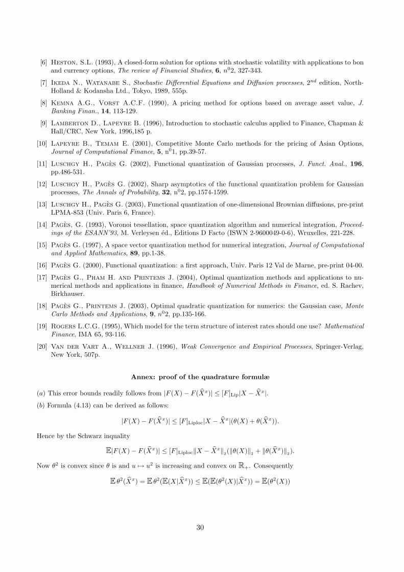
[6] Heston, S.L. (1993), A closed-form solution for options with stochastic volatility with applications to bonand currency options, The review of Financial Studies, 6, n02, 327-343.

[7] Ikeda N., Watanabe S., Stochastic Differential Equations and Diffusion processes, 2nd edition, North-Holland & Kodansha Ltd., Tokyo, 1989, 555p.

[8] Kemna A.G., Vorst A.C.F. (1990), A pricing method for options based on average asset value, J.Banking Finan., 14, 113-129.

[9] Lamberton D., Lapeyre B. (1996), Introduction to stochastic calculus applied to Finance, Chapman &Hall/CRC, New York, 1996,185 p.

[10] Lapeyre B., Temam E. (2001), Competitive Monte Carlo methods for the pricing of Asian Options,Journal of Computational Finance, 5, n01, pp.39-57.

[11] Luschgy H., Pages G. (2002), Functional quantization of Gaussian processes, J. Funct. Anal., 196,pp.486-531.

[12] Luschgy H., Pages G. (2002), Sharp asymptotics of the functional quantization problem for Gaussianprocesses, The Annals of Probability, 32, n02, pp.1574-1599.

[13] Luschgy H., Pages G. (2003), Functional quantization of one-dimensional Brownian diffusions, pre-printLPMA-853 (Univ. Paris 6, France).

[14] Pages, G. (1993), Voronoi tessellation, space quantization algorithm and numerical integration, Proceed-ings of the ESANN’93, M. Verleysen ed., Editions D Facto (ISWN 2-9600049-0-6), Wruxelles, 221-228.

[15] Pages G. (1997), A space vector quantization method for numerical integration, Journal of Computationaland Applied Mathematics, 89, pp.1-38.

[16] Pages G. (2000), Functional quantization: a first approach, Univ. Paris 12 Val de Marne, pre-print 04-00.

[17] Pages G., Pham H. and Printems J. (2004), Optimal quantization methods and applications to nu-merical methods and applications in finance, Handbook of Numerical Methods in Finance, ed. S. Rachev,Birkhauser.

[18] Pages G., Printems J. (2003), Optimal quadratic quantization for numerics: the Gaussian case, MonteCarlo Methods and Applications, 9, n02, pp.135-166.

[19] Rogers L.C.G. (1995), Which model for the term structure of interest rates should one use? MathematicalFinance, IMA 65, 93-116.

[20] Van der Vart A., Wellner J. (1996), Weak Convergence and Empirical Processes, Springer-Verlag,New York, 507p.

Annex: proof of the quadrature formulæ

(a) This error bounds readily follows from |F (X)− F (Xx)| ≤ [F ]Lip|X − Xx|.(b) Formula (4.13) can be derived as follows:

|F (X)− F (Xx)| ≤ [F ]Liploc|X − Xx|(θ(X) + θ(Xx)).

Hence by the Schwarz inquality

E|F (X)− F (Xx)| ≤ [F ]Liploc‖X − Xx‖2(‖θ(X)‖2 + ‖θ(Xx)‖2).

Now θ2 is convex since θ is and u 7→ u2 is increasing and convex on R+. Consequently

E θ2(Xx) = E θ2(E(X|Xx)) ≤ E(E(θ2(X)|Xx)) = E(θ2(X))

30

which completes the proof. Concerning (4.14), one starts from a Taylor expansion, where DF denotes thedifferential of F and ‖ . ‖ the operator norm on L(H),

|F (X)− F (Xx)− (DF (Xx), X − Xx)| ≤ supz∈(X, bXx)

‖DF (z)−DF (Xx)‖|X − Xx|

≤ [DF ]α|X − Xx|1+α.

Consequently∣∣∣EF (X)−EF (Xx)−E

((DF (Xx) |X − Xx)

)∣∣∣ ≤ [DF ]αE |X−Xx|1+α.

NowE

((DF (Xx) |X − Xx)

)= E

((DF (Xx) |E(X − Xx|Xx)

))= E

((DF (Xx) | 0

H

))= 0.

To establish the last quadrature formula, one notes, using the convexity of θ that

supz∈(X, bXx)

‖DF (z)−DF (Xx)‖ ≤ [DF ]Liploc|X − Xx|(θ(Xx) + supz∈(X, bXx)

θ(z))

≤ [DF ]Liploc|X − Xx|(θ(Xx) + max(θ(X), θ(Xx)))

≤ [DF ]Liploc|X − Xx|(2θ(Xx) + θ(X)).

and one concludes as above by combining Jensen and Schwarz Inequalities. ♦

31

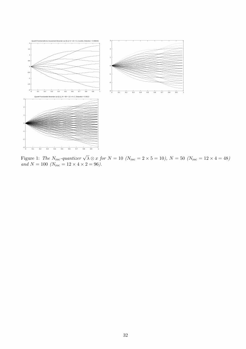
-2

-1.5

-1

-0.5

0

0.5

1

1.5

2

0 0.1 0.2 0.3 0.4 0.5 0.6 0.7 0.8 0.9 1

Quantif Fonctionnelle du mouvement Brownien sur [0,1], N = 10 = 5 x 2 points, Distortion = 0.098446

-3

-2

-1

0

1

2

3

0 0.1 0.2 0.3 0.4 0.5 0.6 0.7 0.8 0.9 1

-3

-2

-1

0

1

2

3

0 0.1 0.2 0.3 0.4 0.5 0.6 0.7 0.8 0.9 1

Quantif Fonctionelle Brownien sur [0,1], N = 96 = 12 x 4 x 2, Distortion = 0.0513

Figure 1: The Nrec-quantizer√λ ⊗ x for N = 10 (Nrec = 2× 5 = 10), N = 50 (Nrec = 12 × 4 = 48)

and N = 100 (Nrec = 12× 4× 2 = 96).

32

0

0.05

0.1

0.15

0.2

0.25

0.3

0.35

0.4

0.45

0.5

0 200 400 600 800 1000

N --> Distortion(N)N --> min(Distortion(k), k<=N)

Figure 2: N 7→ DWN (√λ⊗xopt) and N 7→ min

x∈Opq(N)DWN

(√λ⊗x) = DW

Nrec(√λ⊗xNrec), N = 1, . . . , 1 000.

0

5

10

15

20

25

30

35

40

45

50

1 10 100 1000 10000 100000

N --> 1/min(Distortion(k), k<=N)4*log(x)

Figure 3: logN 7→ 1

DWNrec

(√λ⊗ xNrec)

, N = 1, . . . , 10 000.

33

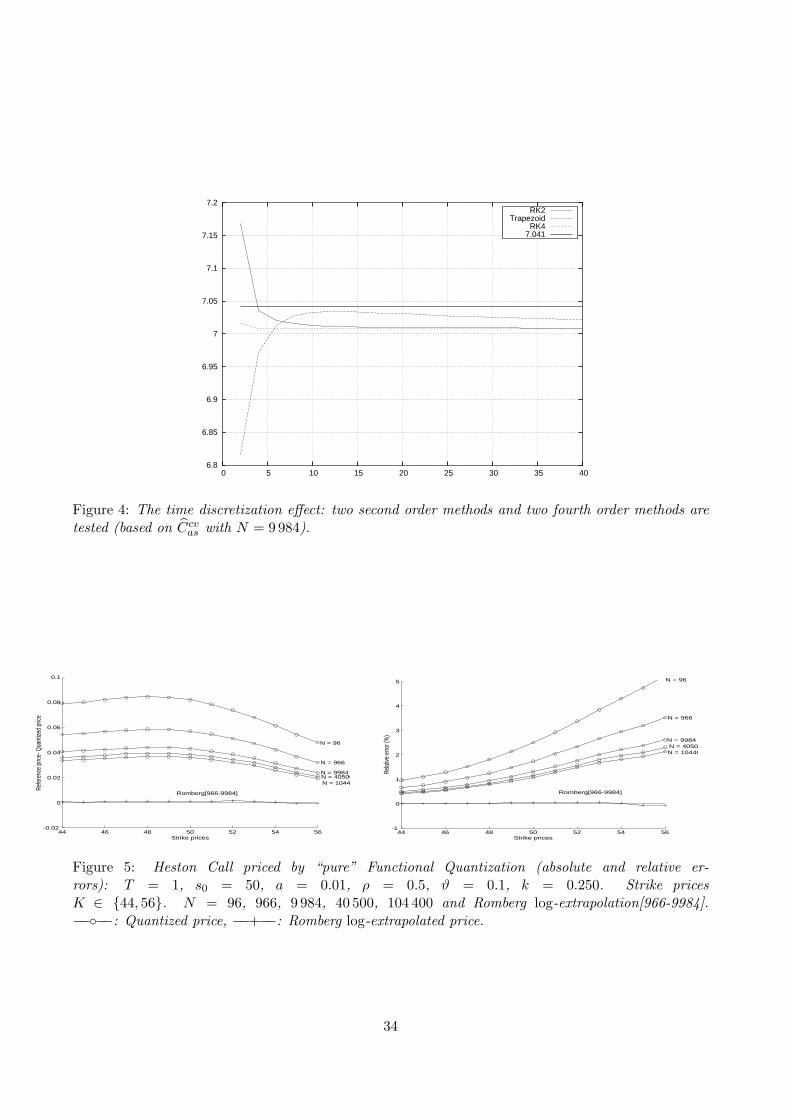
6.8

6.85

6.9

6.95

7

7.05

7.1

7.15

7.2

0 5 10 15 20 25 30 35 40

RK2Trapezoid

RK47.041

Figure 4: The time discretization effect: two second order methods and two fourth order methods aretested (based on Ccvas with N = 9 984).

44 46 48 50 52 54 56-0.02

0

0.02

0.04

0.06

0.08

0.1

Strike prices

Refe

renc

e pr

ice- Q

uant

ized

price

N = 96

N = 966

N = 9984N = 40500N = 104400

Romberg[966-9984]

44 46 48 50 52 54 56-1

0

1

2

3

4

5

Strike prices

Relat

ive e

rror (

%)

N = 96

N = 966

N = 9984

Romberg[966-9984]

N = 40500N = 104400

Figure 5: Heston Call priced by “pure” Functional Quantization (absolute and relative er-rors): T = 1, s0 = 50, a = 0.01, ρ = 0.5, ϑ = 0.1, k = 0.250. Strike pricesK ∈ 44, 56. N = 96, 966, 9 984, 40 500, 104 400 and Romberg log-extrapolation[966-9984].−−−−: Quantized price, −−+−−: Romberg log-extrapolated price.

34

44 46 48 50 52 54 56-0.04

-0.02

0

0.02

0.04

0.06

0.08

Strike prices

Refe

renc

e pr

ice- Q

uant

ized

price

N = 96

N = 966N = 9984N = 40500

N = 104400Romberg[966-9984]

44 46 48 50 52 54 56-5

-4

-3

-2

-1

0

1

Strike prices

Relat

ive e

rror (

%)

N = 96

N = 966

N = 9984N = 40500

N = 104400

Romberg[966-9984]

Figure 6: Heston Call priced by Functional Quantization based on Call-Put Parity equation (absoluteand relative errors): T = 1, s0 = 50, a = 0.01, ρ = 0.5, ϑ = 0.1, k = 0.250. Strike prices K∈ 44, 56,N = 96, 966, 9 984, 40 500, 104 400 and Romberg log-extrapolation[966-9984]. −−−−: Quantized price,−−+−−: Romberg log-extrapolated price.

44 46 48 50 52 54 56-5

0

5

10

15

20x 10

-3

Strike prices

Refe

renc

e pr

ice- Q

uant

ized

price

N = 96

N = 966

N = 9984N = 40500N = 104400

Romberg[966-9984]

44 46 48 50 52 54 56-0.2

0

0.2

0.4

0.6

0.8

1

1.2

Strike prices

Rela

tive

erro

r (%

)

N = 96

N = 966

N = 9984N = 40500N = 104400

Romberg[966-9984]

Figure 7: Heston Call priced by regular Functional Quantization (absolute and relative errors) in theuncorrelated case: T = 1, s0 = 50, a = 0.01, ρ = 0, ϑ = 0.1, k = 0.250. Strike prices K ∈ 44, 56.N = 96, 966, 9 984, 40 500, 104 400 and Romberg log-extrapolation[966-9984]. −−−−: Quantized price,−−+−−: Romberg log-extrapolated price.

44 46 48 50 52 54 560.9

0.92

0.94

0.96

0.98

1

1.02

1.04

1.06

1.08

1.1

Strike prices K

FQ vs

BS

44 46 48 50 52 54 560.9

0.92

0.94

0.96

0.98

1

1.02

1.04

1.06

1.08

1.1

Strike prices K

FQ vs

BS

rho = 0

Figure 8: Is pricing a Heston Call using functional quantization (withRomberg log-extrapolation) more performing than using Black-Scholes formula?−−∗−−: (BS price)/(Heston price), −−−−: (FQ9984 Price)/(Heston price), −−+−−: (FQRomberg log-extrapolated price)/(Heston price).

35