Artificial Neural Networks 2

Morten NielsenBioSys, DTU

Outline

• Optimization procedures – Gradient decent (this you already know)

• Network training– back propagation– cross-validation– Over-fitting– examples

Neural network. Error estimate

I1 I2

w1 w2

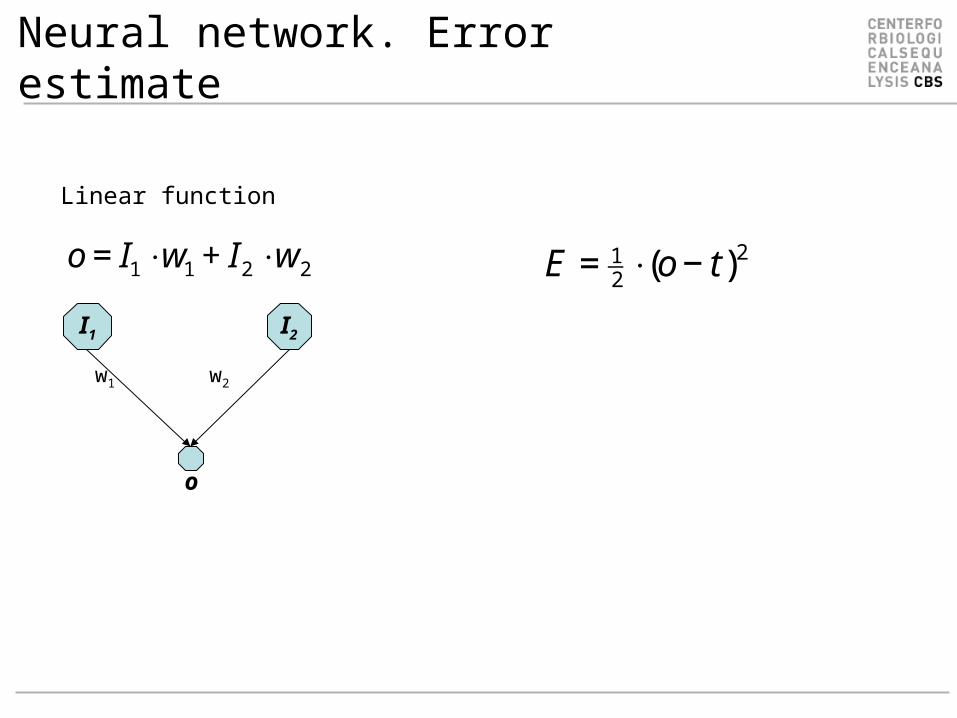
Linear function

€

o = I1 ⋅w1 + I2 ⋅w2

€

E = 12 ⋅(o− t)

2

o

Neural networks

Gradient decent (from wekipedia)

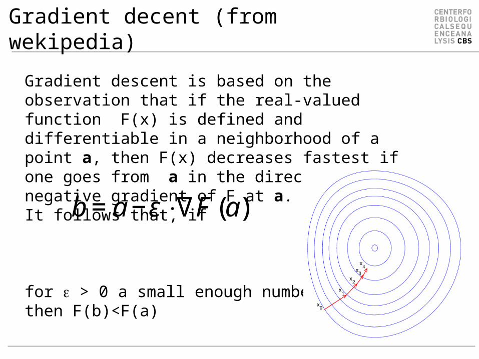
Gradient descent is based on the observation that if the real-valued function F(x) is defined and differentiable in a neighborhood of a point a, then F(x) decreases fastest if one goes from a in the direction of the negative gradient of F at a. It follows that, if

for > 0 a small enough number, then F(b)<F(a)

€

b = a−ε ⋅∇F(a)

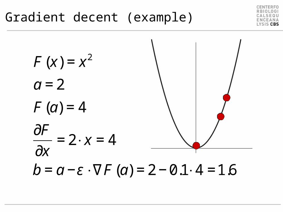
Gradient decent (example)

€

F(x) = x 2

a = 2

F(a) = 4

Gradient decent (example)

€

F(x) = x 2

a = 2

F(a) = 4

∂F

∂x= 2⋅ x = 4

b = a −ε ⋅ ∇F(a) = 2 −0.1⋅ 4 =1.6

Gradient decent. Example

Weights are changed in the opposite direction of the gradient of the error

€

wi' = wi + Δwi

E = 12⋅ (O − t)

2

O = wii

∑ ⋅ Ii

Δwi = −ε ⋅∂E

∂wi= −ε ⋅

∂E

∂O⋅∂O

∂wi−ε ⋅ (O − t)⋅ Ii

I1 I2

w1 w2

Linear function

€

O = I1 ⋅w1 + I2 ⋅w2

o

What about the hidden layer?

€

Δwi = −ε ⋅∂E

∂wi

oi = wijj

∑ ⋅H j

h j = v jkk

∑ ⋅ Ik

€

E = 12 ⋅(O− t)

2

O = g(o),H = g(h)

g(x) =1

1+ e−x

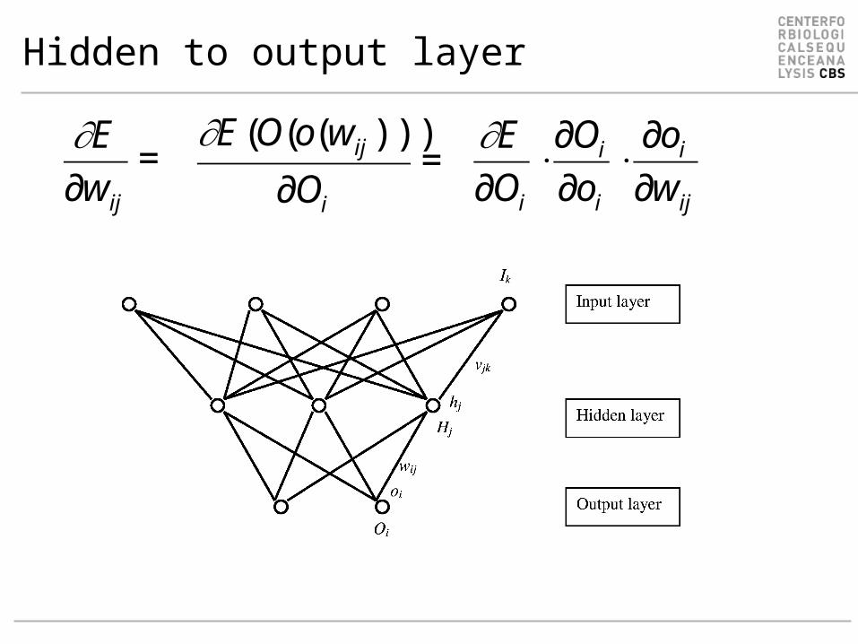
Hidden to output layer

€

∂E∂wij

=

€

∂E∂Oi

⋅∂Oi∂oi

⋅∂oi∂wij

€

∂E(O(o(wij )))∂Oi

=

Hidden to output layer

€

O = g(o)

g(x) =1

1+ e−x

g'(x) =−1

(1+ e−x )2⋅(−e−x )

= (1− g(x)) ⋅g(x)

€

∂E∂wij

=∂E

∂Oi⋅∂Oi∂oi

⋅∂oi∂wij

€

=(O− t) ⋅g'(oi) ⋅H j

€

∂E∂Oi

= (Oi − t)

∂Oi∂oi

=∂g

∂oi= ?

∂oi∂wij

=1

∂wijwlj ⋅

l

∑ H j = H j

Hidden to output layer

€

O = g(o)

g'(o) = (1− g(o))⋅ g(o)

= (1−O)⋅O€

∂E∂wij

=∂E

∂Oi⋅∂Oi∂oi

⋅∂oi∂wij

= (O − t)⋅ (1−O)⋅O⋅H j

€

=(O− t) ⋅g'(oi) ⋅H j

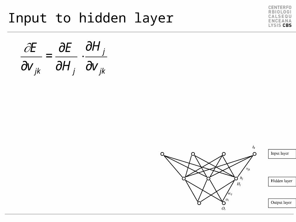
Input to hidden layer

€

∂E∂v jk

=∂E

∂H j

⋅∂H j

∂v jk

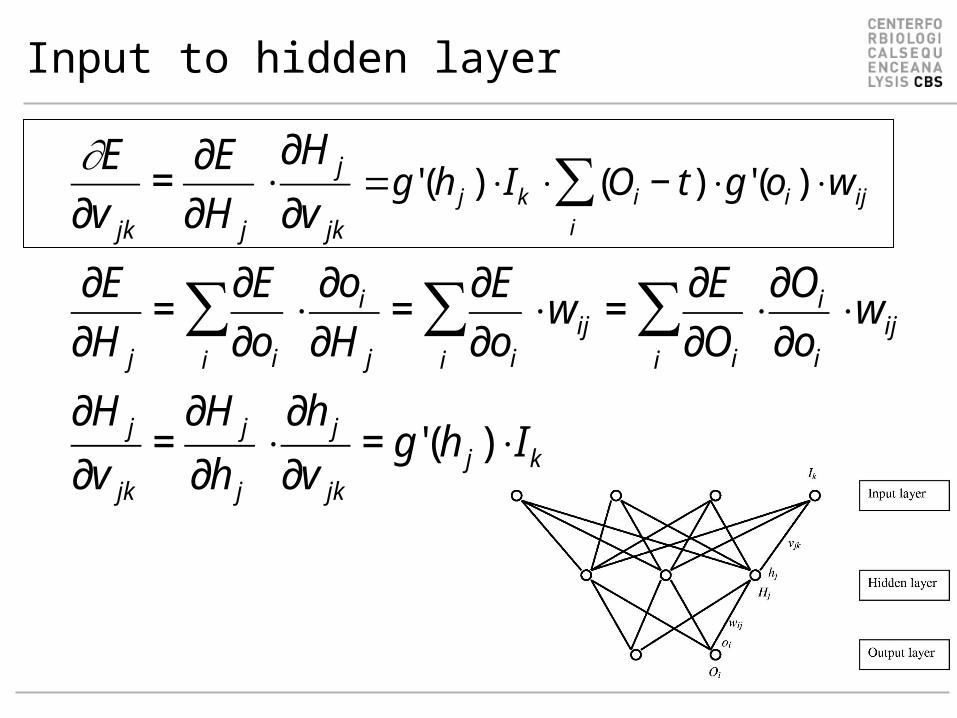
Input to hidden layer

€

∂E∂v jk

=∂E

∂H j

⋅∂H j

∂v jk∂E

∂H j

=∂E

∂oii

∑ ⋅∂oi∂H j

=∂E

∂oii

∑ ⋅wij =∂E

∂Oii

∑ ⋅∂Oi∂oi

⋅wij

∂H j

∂v jk=∂H j

∂h j⋅∂h j∂v jk

= g'(h j ) ⋅ Ik

€

=g'(h j ) ⋅ Ik ⋅ (Oii

∑ − t) ⋅g'(oi) ⋅wij

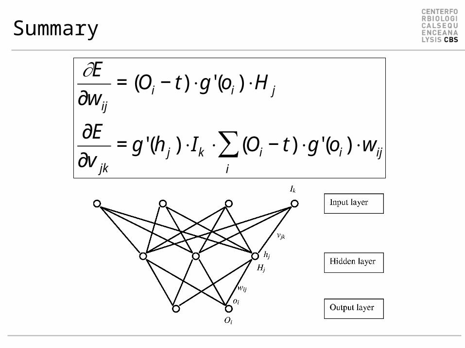
Summary

€

∂E∂wij

= (Oi − t) ⋅g'(oi) ⋅H j

∂E

∂v jk= g'(h j ) ⋅ Ik ⋅ (Oi

i

∑ − t) ⋅g'(oi) ⋅wij

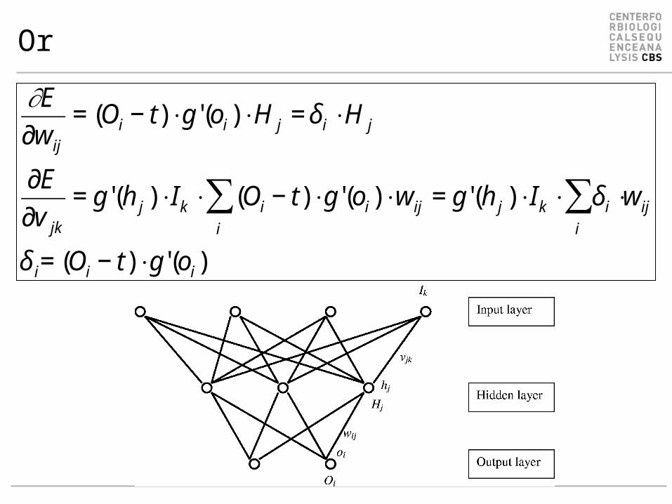
Or

€

∂E∂wij

= (Oi − t) ⋅g'(oi) ⋅H j = δ i ⋅H j

∂E

∂v jk= g'(h j ) ⋅ Ik ⋅ (Oi

i

∑ − t) ⋅g'(oi) ⋅wij = g'(h j ) ⋅ Ik ⋅ δ i ⋅i

∑ wij

δ i= (Oi − t) ⋅g'(oi)

Or

€

∂E∂wij

= δ i ⋅H j = δ i ⋅ x[1][ j]

∂E

∂v jk= g'(h j ) ⋅ Ik ⋅ δi ⋅

i

∑ wij = x[1][ j]⋅(1− x[1][ j]) ⋅ Ik ⋅ δi ⋅i

∑ wij

δ i= (Oi − t) ⋅g'(oi) = (x[2][i]− t) ⋅ x[2][i]⋅(1− x[2][i])

Ii=X[0][i]

Hj=X[1][j]

Oi=X[2][i]

Can you do it your self?

v22=1v12=1

v11=1v21=-1

w1=-1 w2=1

h2

H2

h1

H1

oO

I1=1 I2=1

€

Δwij = −ε ⋅∂E

∂wij;Δv jk = −ε ⋅

∂E

∂v jk∂E

∂wij= (Oi − t) ⋅g'(oi) ⋅H j

∂E

∂v jk= g'(h j ) ⋅ Ik ⋅ (Oi

i

∑ − t) ⋅g'(oi) ⋅wij

g'(x) = (1− g(x)) ⋅g(x)

O = g(o)

What is the output (O) from the network?What are the Δwij and Δvjk values if the target value is 0 and =0.5?

Can you do it your self (=0.5). Has the error decreased?

v22=1v12=1

v11=1v21=-1

w1=-1 w2=1

h2=H2=

H1=

H1=

o=O=

I1=1 I2=1

€

Δw1 = ??Δw2 = ??

€

Δv11 = ??Δv12 = ??

Δv21 = ??

Δv22 = ??

v22=.

v12=V11=

v21=

w1= w2=

h2=H2=

h1=H1=

o=O=

I1=1 I2=1

Before After

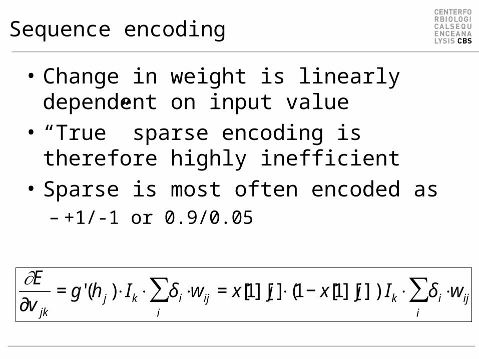
Sequence encoding

€

∂E∂v jk

= g'(h j )⋅ Ik ⋅ δ i⋅i

∑ wij = x[1][ j]⋅ (1− x[1][ j])⋅ Ik ⋅ δ i⋅i

∑ wij

• Change in weight is linearly dependent on input value

• “True” sparse encoding is therefore highly inefficient

• Sparse is most often encoded as– +1/-1 or 0.9/0.05

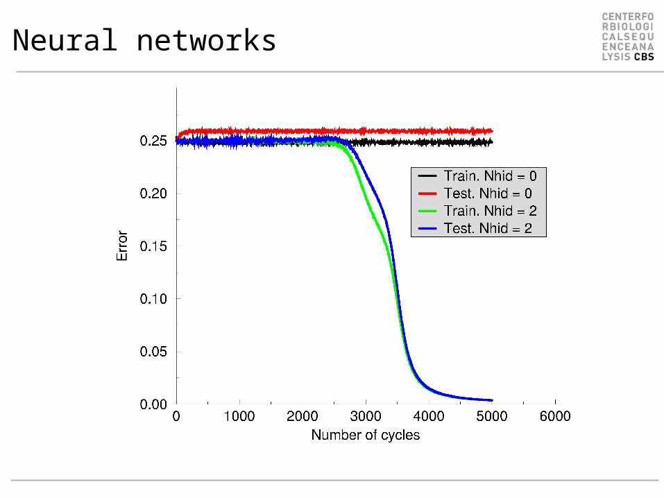
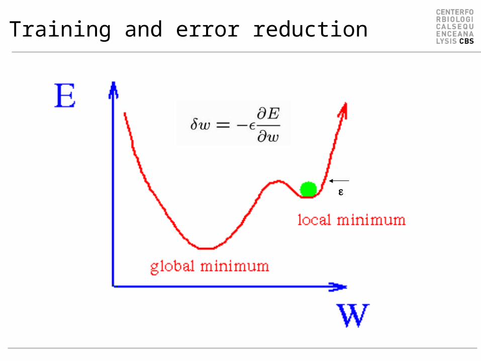
Training and error reduction

Training and error reduction

Training and error reduction

Size matters

• A Network contains a very large set of parameters

– A network with 5 hidden neurons predicting binding for 9meric peptides has more than 9x20x5=900 weights

• Over fitting is a problem• Stop training when test performance is optimal

Neural network training

yearsTem

pera

ture

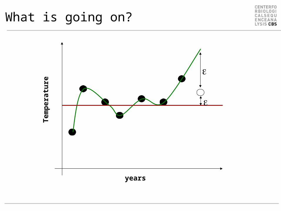
What is going on?

years

Tem

pera

ture

Examples

Train on 500 A0201 and 60 A0101 binding dataEvaluate on 1266 A0201 peptides

NH=1: PCC = 0.77NH=5: PCC = 0.72

Neural network training. Cross validation

120%

220%

320%

420%

520%

Cross validation

Train on 4/5 of dataTest on 1/5=>Produce 5 different neural networks each with a different prediction focus

Neural network training curve

Maximum test set performanceMost cable of generalizing

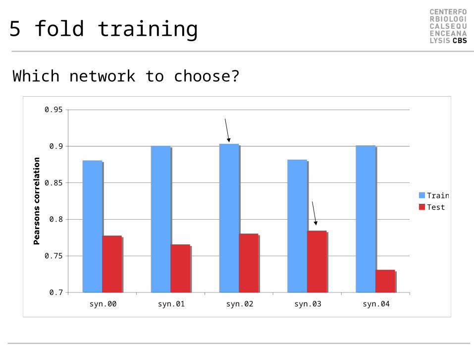
5 fold training

0.7

0.75

0.8

0.85

0.9

0.95

syn.00 syn.01 syn.02 syn.03 syn.04

Pearsons correlation

Train

Test

Which network to choose?

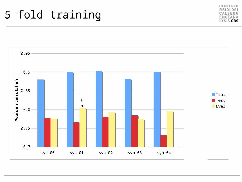
5 fold training

0.7

0.75

0.8

0.85

0.9

0.95

syn.00 syn.01 syn.02 syn.03 syn.04 ens

Pearson correlation

Train

Test

Eval

How many folds?

• Cross validation is always good!, but how many folds?– Few folds -> small training data sets– Many folds -> small test data sets

• Example from before– 560 peptides for training

• 50 fold (10 peptides per test set, few data to stop training)

• 2 fold (280 peptides per test set, few data to train)

• 5 fold (110 peptide per test set, 450 per training set)

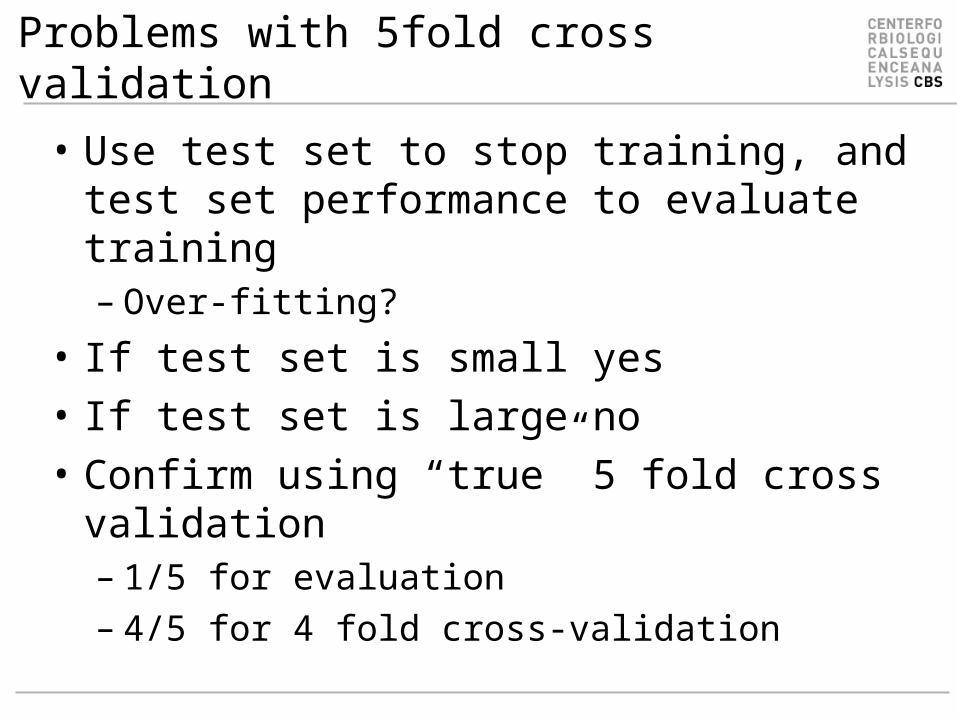
Problems with 5fold cross validation

• Use test set to stop training, and test set performance to evaluate training– Over-fitting?

• If test set is small yes• If test set is large no• Confirm using “true” 5 fold cross

validation– 1/5 for evaluation– 4/5 for 4 fold cross-validation

Conventional 5 fold cross validation

“True” 5 fold cross validation

When to be careful

• When data is scarce, the performance obtained used “conventional” versus “true” cross validation can be very large

• When data is abundant the difference is small, and “true” cross validation might even be higher than “conventional” cross validation due to the ensemble aspect of the “true” cross validation approach

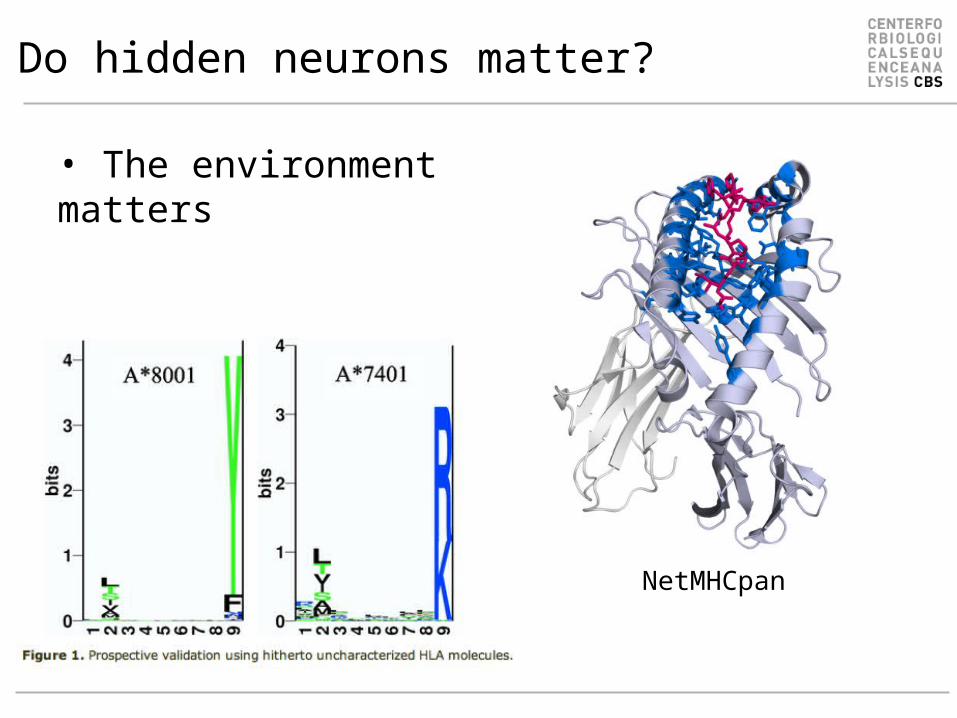
Do hidden neurons matter?

• The environment matters

NetMHCpan

Context matters

• FMIDWILDA YFAMYGEKVAHTHVDTLYVRYHYYTWAVLAYTWY 0.89 A0201• FMIDWILDA YFAMYQENMAHTDANTLYIIYRDYTWVARVYRGY 0.08 A0101• DSDGSFFLY YFAMYGEKVAHTHVDTLYVRYHYYTWAVLAYTWY 0.08 A0201• DSDGSFFLY YFAMYQENMAHTDANTLYIIYRDYTWVARVYRGY 0.85 A0101

Example

Summary

• Gradient decent is used to determine the updates for the synapses in the neural network

• Some relatively simple math defines the gradients– Networks without hidden layers can be solved on

the back of an envelope (SMM exercise)– Hidden layers are a bit more complex, but still ok

• Always train networks using a test set to stop training

• And hidden neurons do matter (sometimes)

And some more stuff for the long cold winter nights

• Can it be made differently?

€

E =1

α⋅(O− t)α

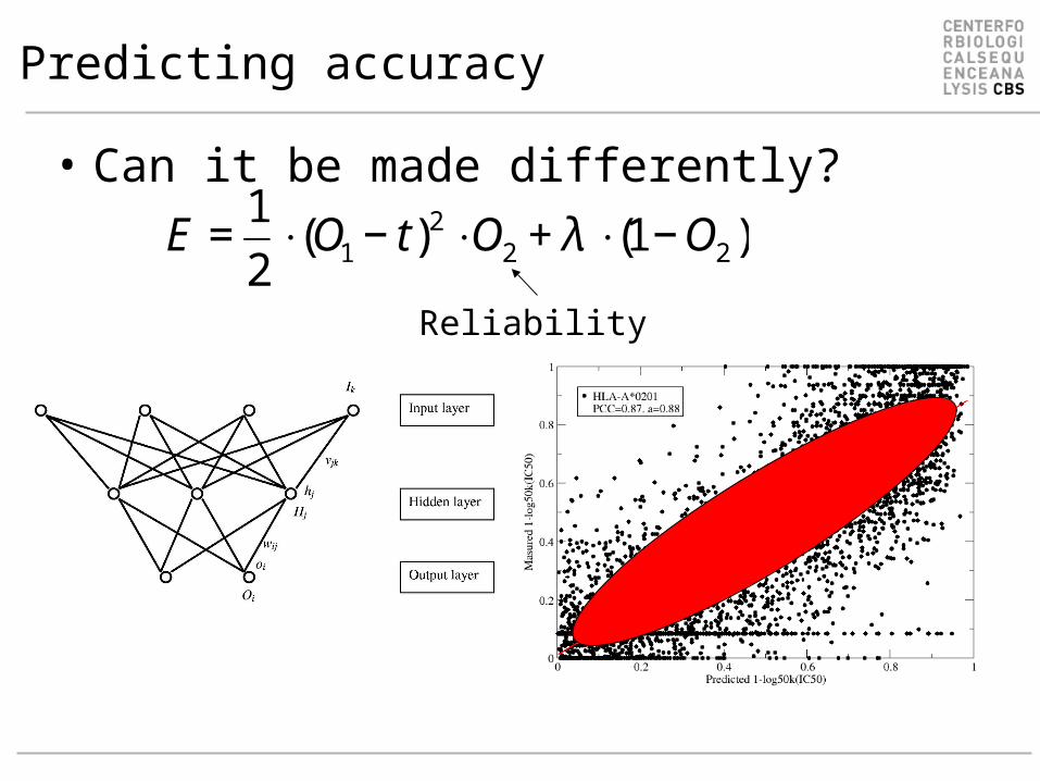
Predicting accuracy

• Can it be made differently?

€

E =1

2⋅(O1 − t)

2 ⋅O2 + λ ⋅(1−O2)

Reliability