Embed Size (px)
Citation preview
PPC Spring 2014 - Interconnection Networks 1
CSCI-4320/6360: Parallel Programming & Computing (PPC)
Interconnection Networks
Prof. Chris CarothersComputer Science Department

2
Interconnection Networks for Parallel Computers
• Interconnection networks carry data between processors and to memory.
• Interconnects are made of switches and links (wires, fiber).
• Interconnects are classified as static or dynamic. • Static networks consist of point-to-point
communication links among processing nodes and are also referred to as direct networks.
• Dynamic networks are built using switches and communication links. Dynamic networks are also referred to as indirect networks.
PPC Spring 2014 - Interconnection Networks
3
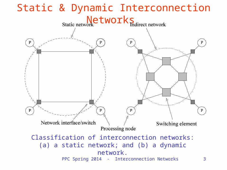
Static & Dynamic Interconnection Networks
Classification of interconnection networks: (a) a static network; and (b) a dynamic network.
PPC Spring 2014 - Interconnection Networks
PPC Spring 2014 - Interconnection Networks 4
Interconnection Networks
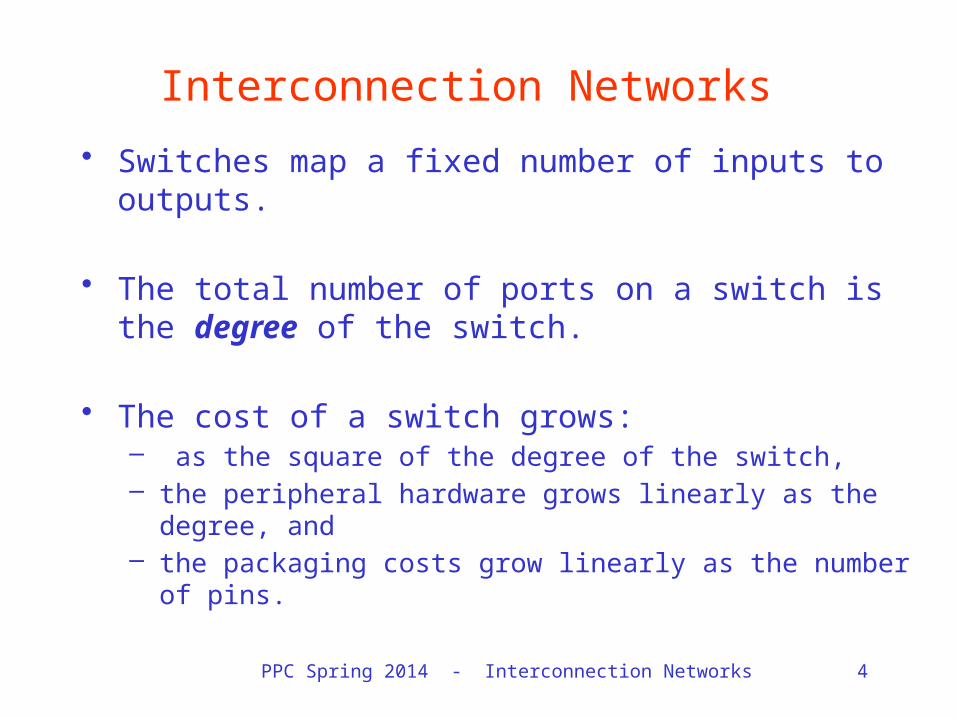
• Switches map a fixed number of inputs to outputs.
• The total number of ports on a switch is the degree of the switch.
• The cost of a switch grows:– as the square of the degree of the switch, – the peripheral hardware grows linearly as the degree,
and – the packaging costs grow linearly as the number of
pins.
PPC Spring 2014 - Interconnection Networks 5
Interconnection Networks: Network Interfaces
• Processors talk to the network via a network interface.
• The network interface may hang off the I/O bus or the memory bus.
• In a physical sense, this distinguishes a cluster from a tightly coupled multicomputer.
• The relative speeds of the I/O and memory buses impact the performance of the network.
PPC Spring 2014 - Interconnection Networks 6
Network Topologies
• A variety of network topologies have been proposed and implemented.
• These topologies tradeoff performance for cost.
• Commercial machines often implement hybrids of multiple topologies for reasons of packaging, cost, and available components.

PPC Spring 2014 - Interconnection Networks 7
Network Topologies: Buses • Some of the simplest and earliest parallel
machines used buses. • All processors access a common bus for
exchanging data. • The distance between any two nodes is O(1) in a
bus. The bus also provides a convenient broadcast media.
• However, the bandwidth of the shared bus is a major bottleneck.
• Typical bus based machines are limited to dozens of nodes. Sun Enterprise servers and Intel Pentium based shared-bus multiprocessors are examples of such architectures.
PPC Spring 2014 - Interconnection Networks 8
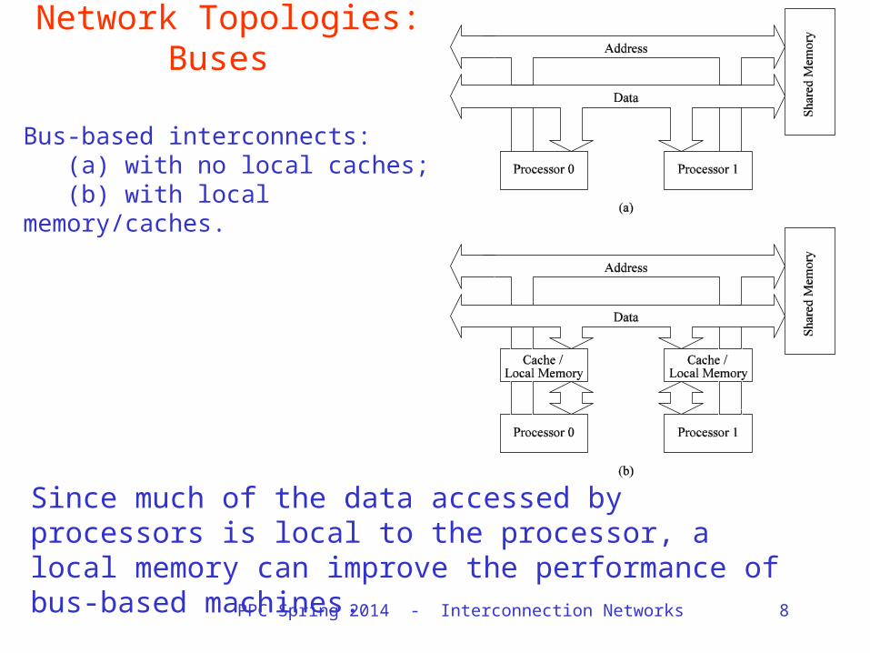
Network Topologies: Buses
Bus-based interconnects:(a) with no local caches; (b) with local
memory/caches.
Since much of the data accessed by processors is local to the processor, a local memory can improve the performance of bus-based machines.

PPC Spring 2014 - Interconnection Networks 9
Network Topologies: Crossbars
A completely non-blocking crossbar network connecting p processors to b memory banks.
A crossbar network uses an p×m grid of switches to connect p inputs to m outputs in a non-blocking manner.

PPC Spring 2014 - Interconnection Networks 10
Network Topologies: Crossbars
• The cost of a crossbar of p processors grows as O(p2).
• This is generally difficult to scale for large values of p.
• Examples of machines that employ crossbars include the Sun Ultra HPC 10000 and the Fujitsu VPP500.
PPC Spring 2014 - Interconnection Networks 11
Network Topologies: Multistage Networks
• Crossbars have excellent performance scalability but poor cost scalability.
• Buses have excellent cost scalability, but poor performance scalability.
• Multistage interconnects strike a compromise between these extremes.

PPC Spring 2014 - Interconnection Networks 12
Network Topologies: Multistage Networks
The schematic of a typical multistage interconnection network.
PPC Spring 2014 - Interconnection Networks 13
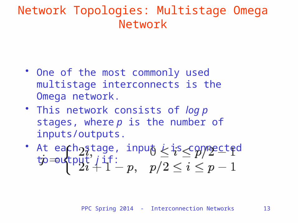
Network Topologies: Multistage Omega Network
• One of the most commonly used multistage interconnects is the Omega network.
• This network consists of log p stages, where p is the number of inputs/outputs.
• At each stage, input i is connected to output j if:
PPC Spring 2014 - Interconnection Networks 14
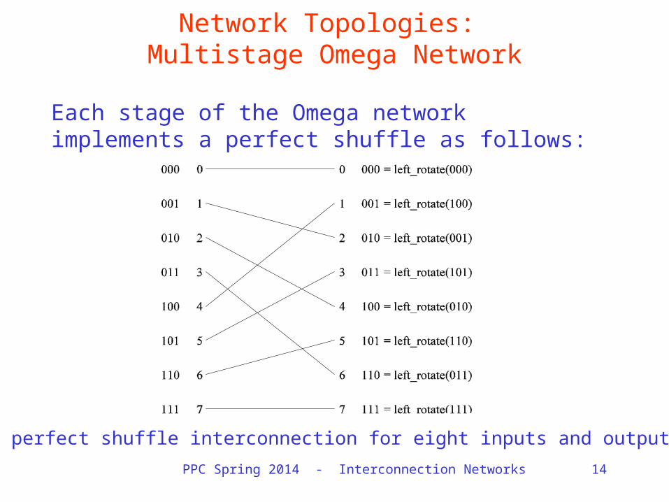
Network Topologies: Multistage Omega Network
Each stage of the Omega network implements a perfect shuffle as follows:
A perfect shuffle interconnection for eight inputs and outputs.
PPC Spring 2014 - Interconnection Networks 15
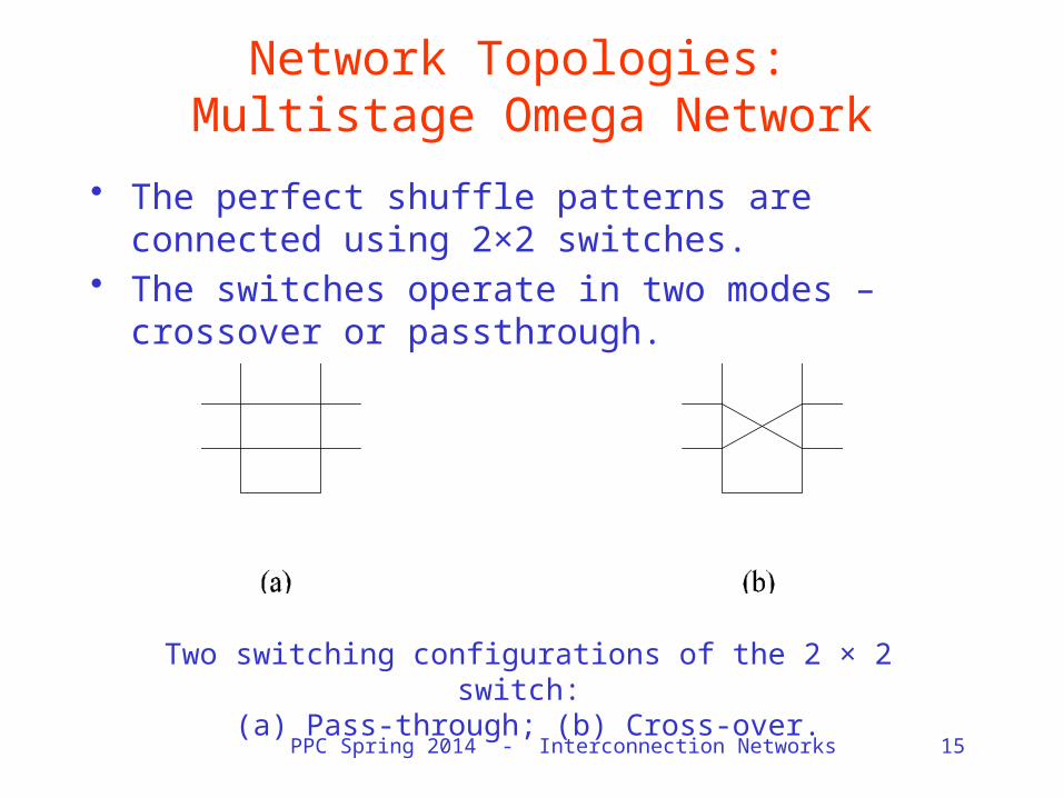
Network Topologies: Multistage Omega Network
• The perfect shuffle patterns are connected using 2×2 switches.
• The switches operate in two modes – crossover or passthrough.
Two switching configurations of the 2 × 2 switch: (a) Pass-through; (b) Cross-over.

PPC Spring 2014 - Interconnection Networks 16
Network Topologies: Multistage Omega Network
A complete omega network connecting eight inputs and eight outputs.
An omega network has p/2 × log p switching nodes, and the cost of such a network grows as (p log p).
A complete Omega network with the perfect shuffle interconnects and switches can now be illustrated:
PPC Spring 2014 - Interconnection Networks 17
Network Topologies: Multistage Omega Network – Routing
• Let s be the binary representation of the source and d be that of the destination processor.
• The data traverses the link to the first switching node. If the most significant bits of s and d are the same, then the data is routed in pass-through mode by the switch else, it switches to crossover.
• This process is repeated for each of the log p switching stages.
• Note that this is NOT a non-blocking switch.

PPC Spring 2014 - Interconnection Networks 18
Network Topologies: Multistage Omega Network – Routing
An example of blocking in omega network: one of the messages
(010 to 111 or 110 to 100) is blocked at link AB.

PPC Spring 2014 - Interconnection Networks 19
Network Topologies: Completely Connected Network
• Each processor is connected to every other processor.
• The number of links in the network scales as O(p2).
• While the performance scales very well, the hardware complexity is not realizable for large values of p.– Well maybe … we’ll see the Sun CLOS switch does scale
to large values of P.• In this sense, these networks are static
counterparts of crossbars.

PPC Spring 2014 - Interconnection Networks 20
Network Topologies: Completely Connected and Star Connected Networks
Example of an 8-node completely connected network.
(a) A completely-connected network of eight nodes; (b) a star connected network of nine nodes.

PPC Spring 2014 - Interconnection Networks 21
Network Topologies: Star Connected Network
• Every node is connected only to a common node at the center.
• Distance between any pair of nodes is O(1). However, the central node becomes a bottleneck.
• In this sense, star connected networks are static counterparts of buses.

PPC Spring 2014 - Interconnection Networks 22
Network Topologies: Linear Arrays, Meshes, and k-d Meshes
• In a linear array, each node has two neighbors, one to its left and one to its right. If the nodes at either end are connected, we refer to it as a 1-D torus or a ring.
• A generalization to 2 dimensions has nodes with 4 neighbors, to the north, south, east, and west.
• A further generalization to d dimensions has nodes with 2d neighbors.
• A special case of a d-dimensional mesh is a hypercube. Here, d = log p, where p is the total number of nodes.

PPC Spring 2014 - Interconnection Networks 23
Network Topologies: Linear Arrays
Linear arrays: (a) with no wraparound links; (b) with wraparound link.

PPC Spring 2014 - Interconnection Networks 24
Network Topologies: Two- and Three Dimensional Meshes
Two and three dimensional meshes: (a) 2-D mesh with no wraparound; (b) 2-D mesh with wraparound link (2-D
torus); and (c) a 3-D mesh with no wraparound.
PPC Spring 2014 - Interconnection Networks 25
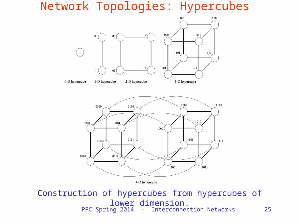
Network Topologies: Hypercubes
Construction of hypercubes from hypercubes of lower dimension.
PPC Spring 2014 - Interconnection Networks 26
Network Topologies: Properties of Hypercubes
• The distance between any two nodes is at most log p.
• Each node has log p neighbors.• The distance between two nodes is given by
the number of bit positions at which the two nodes differ.

PPC Spring 2014 - Interconnection Networks 27
Network Topologies: Tree-Based Networks
Complete binary tree networks: (a) a static tree network; and (b) a dynamic tree network.
PPC Spring 2014 - Interconnection Networks 28
Network Topologies: Tree Properties
• The distance between any two nodes is no more than 2logp.
• Links higher up the tree potentially carry more traffic than those at the lower levels.
• For this reason, a variant called a fat-tree, fattens the links as we go up the tree.
• Trees can be laid out in 2D with no wire crossings. This is an attractive property of trees.
PPC Spring 2014 - Interconnection Networks 29
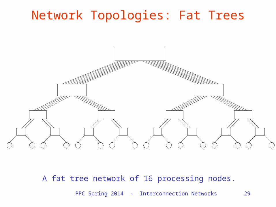
Network Topologies: Fat Trees
A fat tree network of 16 processing nodes.
PPC Spring 2014 - Interconnection Networks 30
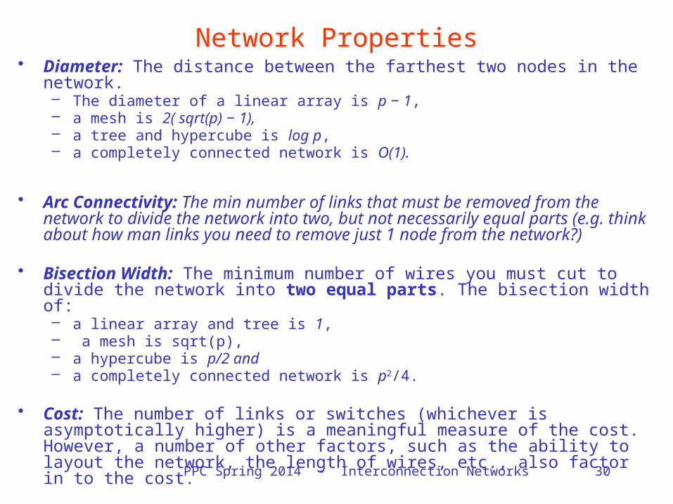
• Diameter: The distance between the farthest two nodes in the network. – The diameter of a linear array is p − 1, – a mesh is 2( sqrt(p) − 1), – a tree and hypercube is log p,– a completely connected network is O(1).
• Arc Connectivity: The min number of links that must be removed from the network to divide the network into two, but not necessarily equal parts (e.g. think about how man links you need to remove just 1 node from the network?)
• Bisection Width: The minimum number of wires you must cut to divide the network into two equal parts. The bisection width of: – a linear array and tree is 1,– a mesh is sqrt(p), – a hypercube is p/2 and – a completely connected network is p2/4.
• Cost: The number of links or switches (whichever is asymptotically higher) is a meaningful measure of the cost. However, a number of other factors, such as the ability to layout the network, the length of wires, etc., also factor in to the cost.
Network Properties
PPC Spring 2014 - Interconnection Networks 31
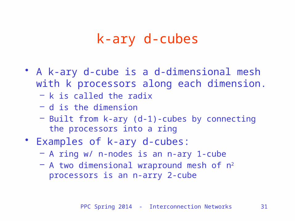
k-ary d-cubes
• A k-ary d-cube is a d-dimensional mesh with k processors along each dimension.– k is called the radix– d is the dimension– Built from k-ary (d-1)-cubes by connecting the
processors into a ring• Examples of k-ary d-cubes:
– A ring w/ n-nodes is an n-ary 1-cube– A two dimensional wrapround mesh of n2 processors
is an n-arry 2-cube

PPC Spring 2014 - Interconnection Networks 32
Evaluating Static Interconnection Networks
Network Diameter BisectionWidth
Arc Connectivity
Cost (No. of links)
Completely-connected
Star
Complete binary tree
Linear array
2-D mesh, no wraparound
2-D wraparound mesh
Hypercube
Wraparound k-ary d-cube

PPC Spring 2014 - Interconnection Networks 33
Evaluating Dynamic Interconnection Networks
Network Diameter Bisection Width
Arc Connectivity
Cost (No. of links)
Crossbar
Omega Network
Dynamic Tree
*This measure appears off..
Our 3 stage, 8 in/out network has 32 links or
p*(log(p) + 1) links

PPC Spring 2014 - Interconnection Networks 34
Communication Costs in Parallel Machines
• Along with idling and contention, communication is a major overhead in parallel programs.
• The cost of communication is dependent on a variety of features including the programming model semantics, the network topology, data handling and routing, and associated software protocols.
PPC Spring 2014 - Interconnection Networks 35
Message Passing Costs in Parallel Computers
• The total time to transfer a message over a network comprises of the following:– Startup time (ts): Time spent at sending and
receiving nodes (executing the routing algorithm, programming routers, etc.).
– Per-hop time (th): This time is a function of number of hops and includes factors such as switch latencies, network delays, etc.
– Per-word transfer time (tw): This time includes all overheads that are determined by the length of the message. This includes bandwidth of links, error checking and correction, etc.

PPC Spring 2014 - Interconnection Networks 36
Store-and-Forward Routing
• A message traversing multiple hops is completely received at an intermediate hop before being forwarded to the next hop.
• The total communication cost for a message of size m words to traverse l communication links is
• In most platforms, th is small and the above expression can be approximated by
PPC Spring 2014 - Interconnection Networks 37
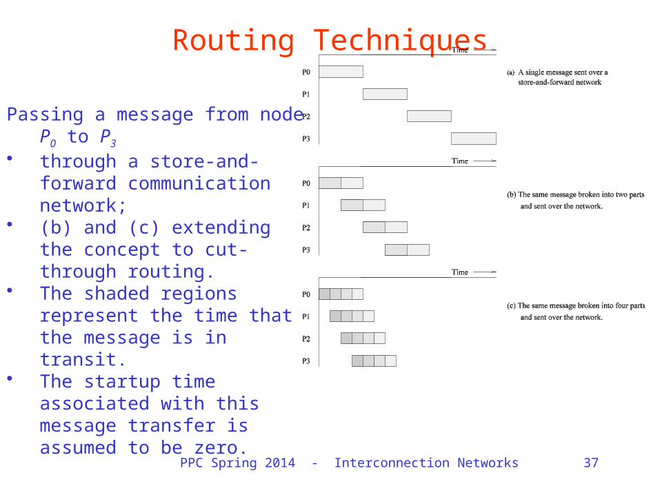
Routing Techniques
Passing a message from node P0 to P3
• through a store-and-forward communication network;
• (b) and (c) extending the concept to cut-through routing.
• The shaded regions represent the time that the message is in transit.
• The startup time associated with this message transfer is assumed to be zero.

PPC Spring 2014 - Interconnection Networks 38
Packet Routing
• Store-and-forward makes poor use of communication resources.
• Packet routing breaks messages into packets and pipelines them through the network.
• Since packets may take different paths, each packet must carry routing information, error checking, sequencing, and other related header information.
• The total communication time for packet routing is approximated by:
• The factor tw accounts for overheads in packet headers.

PPC Spring 2014 - Interconnection Networks 39
Cut-Through Routing • Takes the concept of packet routing to an
extreme by further dividing messages into basic units called flits.
• Since flits are typically small, the header information must be minimized.
• This is done by forcing all flits to take the same path, in sequence.
• A tracer message first programs all intermediate routers. All flits then take the same route.
• Error checks are performed on the entire message, as opposed to flits.
• No sequence numbers are needed.

PPC Spring 2014 - Interconnection Networks 40
Cut-Through Routing
• The total communication time for cut-through routing is approximated by:
• This is identical to packet routing, however, tw is typically much smaller.
PPC Spring 2014 - Interconnection Networks 41
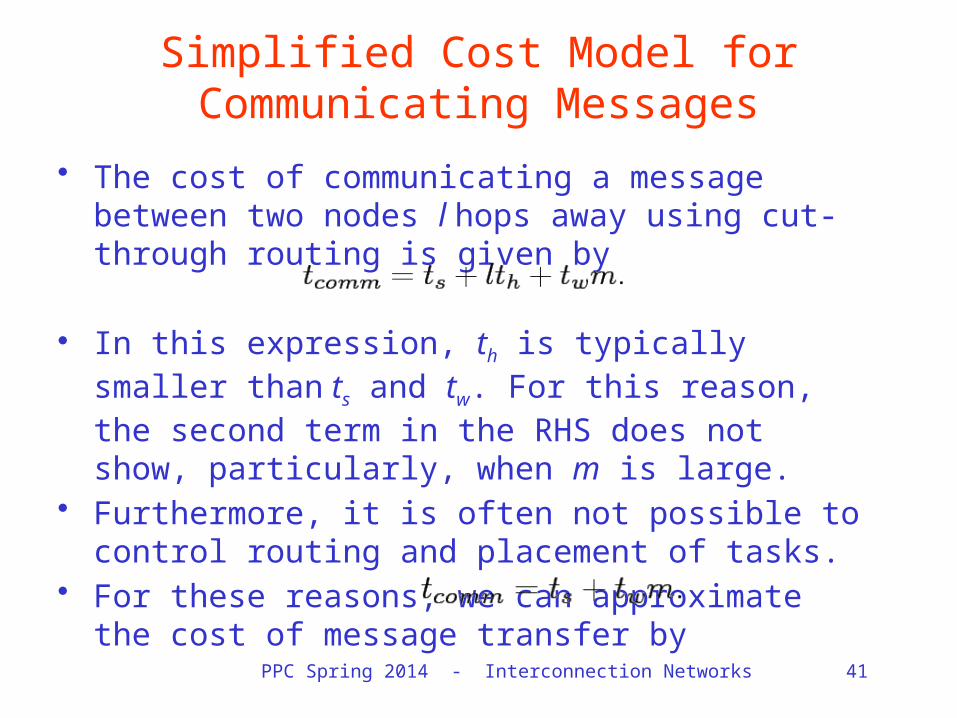
Simplified Cost Model for Communicating Messages
• The cost of communicating a message between two nodes l hops away using cut-through routing is given by
• In this expression, th is typically smaller than ts and tw. For this reason, the second term in the RHS does not show, particularly, when m is large.
• Furthermore, it is often not possible to control routing and placement of tasks.
• For these reasons, we can approximate the cost of message transfer by
PPC Spring 2014 - Interconnection Networks 42
Simplified Cost Model for Communicating Messages
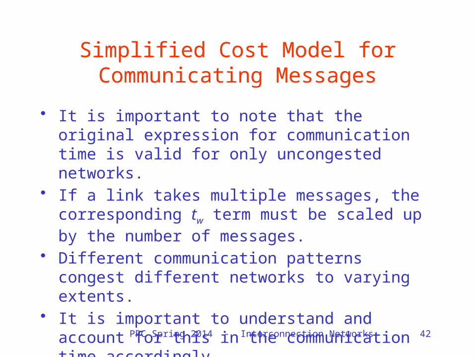
• It is important to note that the original expression for communication time is valid for only uncongested networks.
• If a link takes multiple messages, the corresponding tw term must be scaled up by the number of messages.
• Different communication patterns congest different networks to varying extents.
• It is important to understand and account for this in the communication time accordingly.
PPC Spring 2014 - Interconnection Networks 43
Routing Mechanisms for Interconnection Networks
• How does one compute the route that a message takes from source to destination? – Routing must prevent deadlocks - for this reason, we
use dimension-ordered or e-cube routing.
– Routing must avoid hot-spots - for this reason, two-step routing is often used. In this case, a message from source s to destination d is first sent to a randomly chosen intermediate processor i and then forwarded to destination d.

PPC Spring 2014 - Interconnection Networks 44
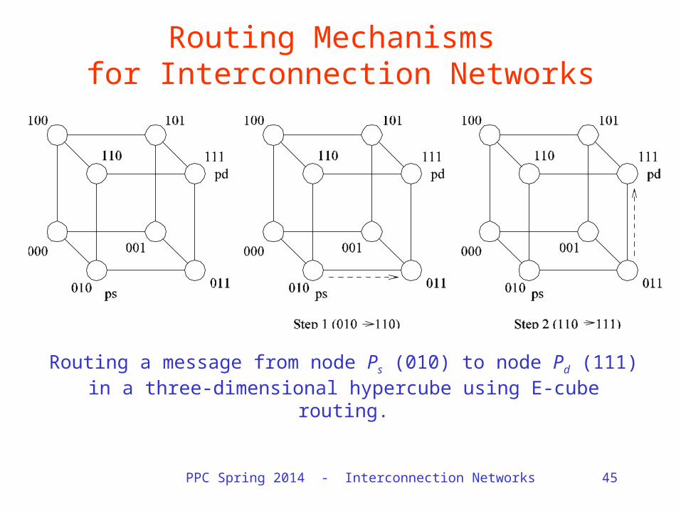
E-Cube Routing
• Let Ps and Pd be the labels of the source and destination nodes of a p-dimensional hypercube..
• Min distance between nodes is Ps XOR Pd• Algorithm
– Ps computes Ps XOR Pd– Ps sends msg along dimension k where k is the LS
NON-ZERO bit position in Ps XOR Pd– At each next step, Pi computes Pi XOR Pd and
forward the message along the dimension of the LS NON-ZERO bit.
PPC Spring 2014 - Interconnection Networks 45
Routing Mechanisms for Interconnection Networks
Routing a message from node Ps (010) to node Pd (111) in a three-dimensional hypercube using E-cube routing.