PowerScope: Early Event Detection andIdentification in Electric Power Systems

Yang Weng1⋆, Christos Faloutos2, and Marija Ilic1

1 Department of Electrical and Computer Engineering, Carnegie Mellon University,Pittsburgh, PA, 15213, USA, yangweng@andrew.cmu.edu, milic@ece.cmu.edu

2 School of Computer Science, Carnegie Mellon University, Pittsburgh, PA, 15213,USA, christos@cs.cmu.edu

Abstract. This paper is motivated by major needs for fast and accu-rate on-line data analysis tools in the emerging electric energy systems,due to the recent penetration of distributed green energy, distributed in-telligence, and plug-in electric vehicles. Instead of taking the traditionalcomplex physical model based approach, this paper proposes a data-driven method, leading to an effective early event detection approachfor the smart grid. Our contributions are: 1) introducing the early eventdetection problem, 2) providing a novel method for power systems dataanalysis (PowerScope), i.e. finding hidden power flow features which aremutually independent, 3) proposing a learning approach for early even-t detection and identification based on PowerScope. Although machinelearning approaches is adopted, our approach does account for physicalconstraints to enhance performance. By using the proposed early even-t detection method, we are able to obtain an event detector with highaccuracy but significantly reduce the detection time. Such result showsthe potential for sustainable grid services through real-time data analysisand control.

Keywords: power systems, smart grid, early event detection, data min-ing, nonparametric method, machine learning

1 Introduction

Regarded as a seminal national infrastructure, the electric power grid provides aclean, convenient, and relatively easy way to transmit electricity to both urbanand suburban areas. Therefore, it is critical to operate the electric power systemsin a reliable and efficient way. However, the grid often exhibits vulnerability topenetrations and disruptive events, such as blackouts. Interruptions of electric-ity service or extensive blackouts are known contributors to physical hardwaredamages, unexpected interruption of normal work, and subsequent economicloss. To monitor potential problems [1], hidden state information is usually ex-tracted from redundant measurement data in the Supervisory Control And Data

⋆ Yang Weng is supported by an ABB Fellowship.

II

Acquisition (SCADA) system using static state estimation (SE) [2]; the resultsof SE are then used for on-line assessment of abnormal event [3] detection.

However, such a static model-based event detection method often causes asignificant gap in performance between the state-of-the-art methods and the de-sired informative data exploration. In particular, with recent and ongoing mas-sive penetration of renewable energy, traditional methods are unable to track andmanage increasing uncertainties inherently associated with these new technolo-gies [4]. Further, President Obama’s goal of putting one million electric vehicleson the road by 2015 will also contribute to the grid architecture shift. Because ofthe unconventional characteristics of these technologies, faster and more accurateevent detector must be conducted for the robust operation of smart grid.

On the other hand, more sensors [5, 6], high performance computers, andstorage devices are deployed over the power grid in recent years, which createsan enormous amount of data that is unbelievable in the past. Utilizing thesedata can be regarded as a perfect opportunity to test and resolve the problemstated above. Notably, learning from the data to deal with uncertainties hasbeen widely recognized as a key player in achieving the core design of WideArea Monitoring, Control and Protection (WAMPAC) systems, which centerson efficient and reliable operations [7].

In this paper, we propose a fast event detection method caller early eventdetector. We will use historical data to help predict the complete event sequencebased on a partial measurement sequence. Such short sequence may seem to benegligible from an system operator’s field operation, but it contains rich infor-mation about what is going on next based on the historical data. As processinghistorical data requires huge computational time, we start with analyzing thespeedup possibility by looking into power grid data structure via Singular ValueDecomposition (SVD) [8] and Independent Component Analysis (ICA). Sucha method is named PowerScope in this paper. Based on our understanding ofthe possibility of dimension reduction and independent power flow component, adata-driven early event method is then proposed in a nonparametric model [9].To embed power flow equation inside our detector, a polynomial kernel is usedin the regression process. Our simulation over standard IEEE test cases showedthat one can detect events much faster rather than waiting to see the completeevent shows up. Such an algorithms can form the basis for smart grids analysis byconverting large complex system analysis into small physically meaningful inde-pendent components to enhance system operation in a predictable ways. Finally,two more applications based on PowerScope are proposed: (1) geographical-plotfor visualization and (2) greenness for grid evaluation.

The rest of this paper is organized as follows: In Section 2, we review thepower systems model and define the problem. In Section 3, we first conduct adata analysis for power systems; subsequently, we propose to use independentcomponents with kernel ridge regression to conduct efficient early event detec-tion. Two other applications based on data analysis are described in Section 4. InSection 5, we illustrate the simulation results. Finally, we conclude our analysisin Section 6.

III

2 Power Systems Data and Problem Definition

2.1 Power Systems Data

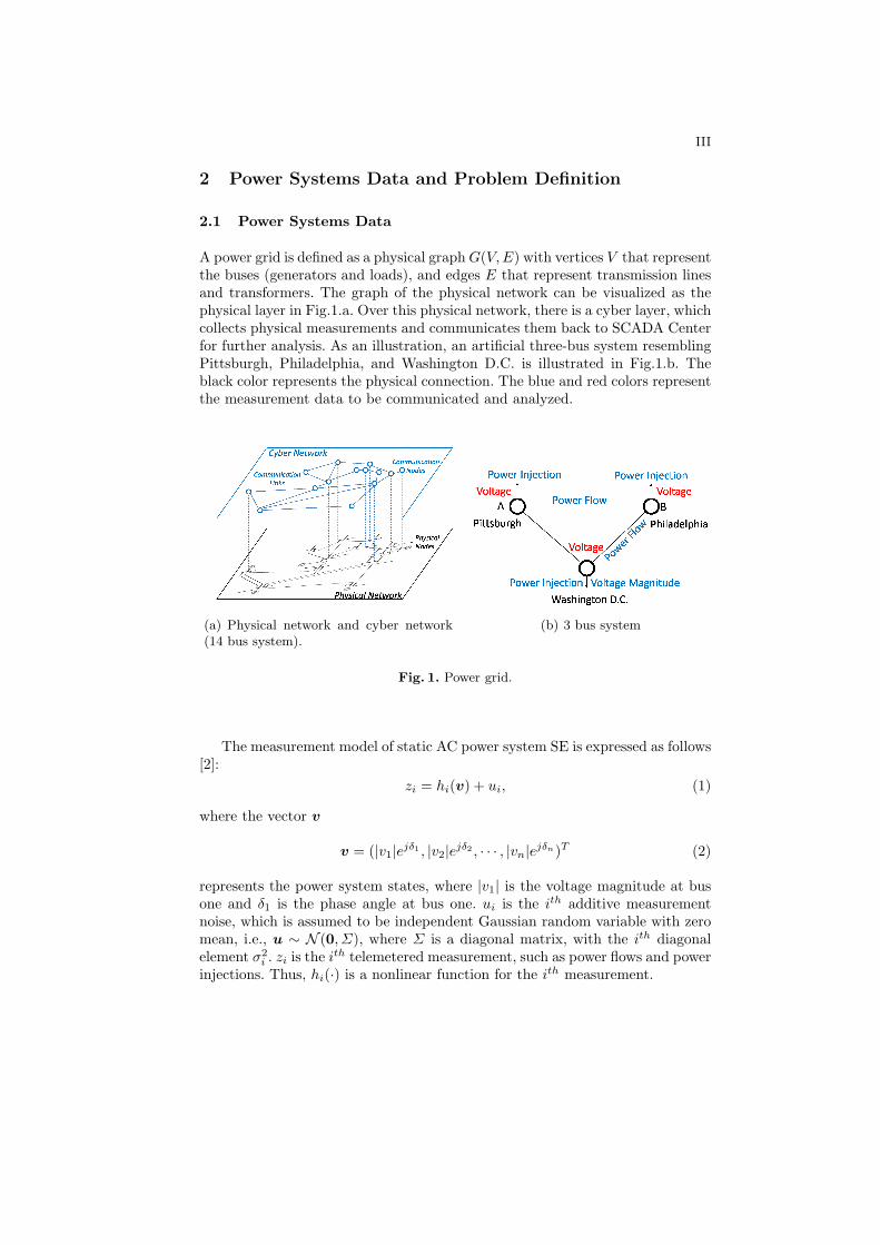
A power grid is defined as a physical graphG(V,E) with vertices V that representthe buses (generators and loads), and edges E that represent transmission linesand transformers. The graph of the physical network can be visualized as thephysical layer in Fig.1.a. Over this physical network, there is a cyber layer, whichcollects physical measurements and communicates them back to SCADA Centerfor further analysis. As an illustration, an artificial three-bus system resemblingPittsburgh, Philadelphia, and Washington D.C. is illustrated in Fig.1.b. Theblack color represents the physical connection. The blue and red colors representthe measurement data to be communicated and analyzed.

(a) Physical network and cyber network(14 bus system).

(b) 3 bus system

Fig. 1. Power grid.

The measurement model of static AC power system SE is expressed as follows[2]:

zi = hi(v) + ui, (1)

where the vector v

v = (|v1|ejδ1 , |v2|ejδ2 , · · · , |vn|ejδn)T (2)

represents the power system states, where |v1| is the voltage magnitude at busone and δ1 is the phase angle at bus one. ui is the ith additive measurementnoise, which is assumed to be independent Gaussian random variable with zeromean, i.e., u ∼ N (0, Σ), where Σ is a diagonal matrix, with the ith diagonalelement σ2

i . zi is the ith telemetered measurement, such as power flows and power

injections. Thus, hi(·) is a nonlinear function for the ith measurement.

IV

2.2 Problem Definition

Instead of conducting model based analysis over a single time slot, we aim at per-forming historical data-driven early event detection and identification for powersystems in this paper. We consider a sequence of historical SCADA measure-ments obtained every 2 seconds (or shorter, when faster devices such as PhasorMeasurement Units are available.). These measurements are represented as a dis-crete time sequence {z1, z2, · · · , zk, · · · , zK}. For instance each column of Fig.2represents a measurement set at a time slot. Besides, historical events, such asevent with type A, are associated with corresponding time slots. We assumethat a new event can only be identified after a relative long period of time. Theproblem we try to solve here is to use the historical data to detect and identifya new event as soon as possible. The formal problem definition is:

Fig. 2. Problem definition.

– Problem Name: Early Event Detection and Identification– Given:

• a sequence of long historical measurements {z1,z2, · · · , zk, · · · , zK}.• a list of events associated with time stamps.

– Find: a data driven event detector and identify the event type as fast aspossible.

3 Proposed Early Event Detection Method

First, we observed that power systems exhibit strong periodicity with inertial(Fig.3) and that similar events usually produce similar measurements sequences.Reversely, if a similar measurement sequence is detected, a similar event is high-ly likely to incur. Therefore, we propose to first collect a similar measurementsequence in the historical database with respect to the current measurementsequence. To make it robust, a group of similar sequences rather than one mea-surement sequence shall be collected. A direct way is to report an event, oncewe find that similar historical measurement sequences are frequently associated

V

Fig. 3. Power system pattern.

with an (abnormal) event. However, such a method not only need to wait untilwhole event completes, but also requires long exhaustive search time.

To reduce the nearest neighbor sequences search time, we propose to use theICA to map the data into lower dimensional space as illustrated in Fig.4. Toconduct the detection process earlier, we employ prediction techniques based onkernel ridge regression. Thereafter we use the current measurement data togetherwith the predicted future measurements for event identification.

Therefore, the proposed algorithm can be described as:

– Step 1: use ICA to map the data onto low dimensional space.– Step 2: nearest neighbor sequences search over low dimensional space.– Step 3: kernel ridge regression: predict future measurements with historical

nearest neighbor sequences.– Step 4: use the current measurement sequence in combination with the pre-

dicted measurement sequence to find another nearest neighbor sequence inthe database.

– Step 5: declare the event associated with the historical neighbor sequence.

In below, we introduce the dimension reduction, nearest neighbor search, andkernel ridge regression for prediction.

3.1 Dimension Reduction-PowerScope

Singular Value Decomposition The power system has enormous amount ofbuses. Therefore, directly working on the grid data is prohibitive due to the curseof dimensionality. However, as the electrical power system exhibits periodicity(i.e. Fig.5.a), we expect the measurement data to be highly clustered as to cre-ating the possibility for great dimension reduction for measurement data. In thispaper, we propose to conduct SVD over the historical data to see if dimensionreduction is possible. We collect one year data of a power grid. As the data iscollected every 5 minutes, we obtain K = 47520 data points. The power grid

VI

Fig. 4. Dimension reduction.

has 300 buses, representing 300 nodes connected via 460 branches. In each da-ta point, we have multiple measurements distributed on the buses (nodes) andtransmission lines (branches). In our analysis, we have different measurements,namely the power flow measurements and power injection measurements. Theycontributed 1073 measurements per time slot over a period of one year, whichare used to form the historical measurement matrix Z = [z1, z2, · · · , zK ].

The SVD decomposition below is then applied to the historical measurementmatrix Z.

Z = U × S × V ′, (3)

where the diagonal entries of S are known as the singular values of S. U andV are unitary matrices [10]. By plotting the singular values of Z in Fig.5.awith a log− log scale, only 8 significant singular values occurred. Besides, inFig.5.b, we show the result of mapping the historical data onto certain twodimensional features (two left-singular vectors of U) associated with significantsingular values. This verifies our expectation of clustered data points.

3.2 Independent Component Analysis

To further analyze the pattern of the power grid data, we conduct IndependentComponent Analysis (ICA) on the same data source as used in the analysis ofSection 3.1. Differently, the same data is now represented by a new matrix B.Each row now represents a daily power injection, or power flow measurementswithin a particular day. In ICA, the task is to transform the observed data Binto maximally independent components s using a linear static transformationW as s = Wb [11]. As a result, the components bi are generated as a sum of theindependent components sk, k = 1, · · · , n:

bi = ai,1s1 + · · ·+ ai,ksk + · · ·+ ai,nsn, (4)

weighted by the mixing weights ai,k.

VII

(a) singular values. (b) measurement data clustering.

Fig. 5. singular value decomposition (SVD).

To implement ICA into our analysis, we use the software Fastica Packagefor MATLAB [12]. As an illustration, Fig.6.a shows a result of applying theFastica package over two daily signals. As the two signals exhibit high powerusage during the day, independent component analysis converted them into sig-nals with in-common and distinctive features on the right of Fig.6.a. The bluesolid line represents basic power consumption, which corresponds to high powerusage/generation in day time. The green dash line represents randomness on topof the blue solid line. Fig.6.b shows the result of applying Fastica to matrix B.The top two sub-figures represent two peaks of power consumption hours, 8 a.m.and 2 p.m. The first sub-figure in the second row represents high power usagein the day time. “−6” on the vertical coordinate represents high power usage inday time. The second figure in the second row represents two power flow changeshappen at 6 a.m. and 6 p.m. The rest three sub-figures depict randomness withinthe grid. We call such a decorrelation process of the power system data “Power-Scope”. In the following, the seven independent components are used data-drivenearly event detection, because they are compact representations of the physicallymeaningful signals, which can be used for computationally-tractable inferences.More PowerScope-based applications will be introduced in Section 4.

3.3 Nearest Neighbors Search

For simplicity, in this subsection, we use formula (5) to find K nearest neighborsequences in the historical database.

s = arg min|s|=p

d(s) =∑k∈s

||zseqcurrent − zseq

k ||22, k ≤ K, k ∈ N (5)

i.e., minimizing sum distance function d(s). Here K is the number of total datapoints in the database. N represents the set of natural numbers. k represents aparticular index for a data point. As a result, zseq

k indicates the measurement se-quence starting from the time slot of index k with a length b. Finally, p indicatesthe cardinality of the set s. Essentially, during the search step, the algorithm

VIII

0 5 10 15 20 250.4

0.6

0.8

1

1.2

1.4

1.6

1.8

2

2.2

2.4

0 5 10 15 20 25−2

−1

0

1

2

3

4

5

(a) Separation of two signals.

0 10 20 30−10

−5

0

0 10 20 300

5

10

0 10 20 30−6

−4

−2

0 10 20 30−25

−20

−15

0 10 20 30−10

−5

0 10 20 30−20

−18

−16

0 10 20 30

−4

−2

0

(b) Major independent components.

Fig. 6. Independent Component Analysis

simply looks for an index set s with p elements which represents a group of mea-surement sequences that have nearer distance to the current sequence zseq

current.

3.4 Kernel ridge regression

After obtaining the minimum distance index set s, this subsection aims to use thecomplete historical measurement sequences as well as the current partial mea-surement sequence to obtain a good prediction for subsequent future sequences.Then we have an understanding what is the potential event that is going on,rather than waiting to the end of it. Afterwards, the complete sequence is usedto identify the associating event and report earlier. Such a process can be illus-trated in Fig.7. To simplify the computation process, each historical measure-ment sequence is vectorized into a single column vector. As a result, each sliceof matrix in Fig.7 will be represented as a vector. For example, the ith histori-cal measurement sequence zseq

i on the top left will be denoted as a vector wi.The ith historical measurement sequence on the top right will be vectorized asa vector yi. The current sequence on the bottom left zseq

current is vectorized by avector wcurrent. The future measurement sequence to be predicted is vectorizedby a vector yfuture

Ridge regression: We explain the process by first considering the Normalmodel below, which is a popular discriminative model with unknown hyper-parameters q and Σd:

y|w : N(qTw,Σd). (6)

To identify such discriminative model for our inference, a regularized (ridgeregression) estimator in (7) is commonly used:

q = argminq

h∑i=1

(yi − qTwi)2 + 2γ||q||2 (7)

IX

Fig. 7. Kernel ridge regression for prediction.

For the Normal model, we assume with the historical data are stored in

Wmat = (w1,w2, · · · ,wh), Y Tmat = (y1,y2, · · · ,yh), (8)

where the subscript h is the total number of chosen neighbor measurement sets,we can obtain a closed-form solution:

q = (WmatWTmat + 2γI)−1Wmaty. (9)

(The unknown hyper-parameter Σd has been absorbed into the penalty con-stant γ.) Notice that due to the ridge regularization (since γ > 0), WmatW

Tmat +

2γI ≽ 2γI ≻ 0, so that this matrix is always invertible. Thus, the regularizedestimator always exists. Once the hyper-parameter q is estimated, it can be usedfor the Bayesian inference to calculate the future measurement vector estimateyBfuture as follows:

yB = qTwcurrent = yTcurrentW

Tmat(WmatW

Tmat+2γI)−1wcurrent = yT

currentT (10)

Further by employing the Matrix Inversion Lemma (A+BDC)−1 = A−1 −A−1B(D−1 + CA−1B)CA−1 to expand the inversion above, we can obtain thealternative form of T , which can further simplify the computation:

T = WTmat(WmatW

Tmat + 2γI)−1wcurrent = (WT

matWmat + 2γI)−1WTmatwcurrent

(11)where

WTmatWmat = (w1,w2, · · · ,wn)

T (w1,w2, · · · ,wn)

=

wT1 w1 . . . wT

1 wn

.... . .

...wT

nw1 . . . wTnwn

(12)

X

WTmatwcurrent = (w1,w2, · · · ,wn)

Twcurrent

=

wT1 wcurrent

...wT

nwcurrent

. (13)

Note that the matrix WTmatWmat appears in the calculation (11), as opposed

to the original calculation (11) involving WmatWTmat, which creates the potential

to reduce computation cost.

The Kernel trick for Normal Discriminative model: A high-dimensionalmapping w = f(u) exists for the problem presented above, from which the innerproduct wT

i wj = (f(ui))T f(uj) can be calculated by a kernel K(·, ·), as below,

wTi wj = K(ui,uj). (14)

Be aware that kernel calculation uses only the (low-dimensional) u’s, ratherthan the high-dimensional w’s. Therefore, the computational complexity of cal-culating the inner products in (12) and (13) is low, even though dim(wcurrent)itself may represent a large number. This idea of using a cost-effective kernelcalculation to implement a high-dimensional Normal model is called ‘the kerneltrick’. In this paper, we employ the following kernel forms as candidates.

– Homogeneous polynomial: K(ui,uj) = (uTi uj)

d.– Inhomogeneous polynomial: K(ui,uj) = (1 + uT

i uj)d.

– Gaussian (Radial Basis function): K(ui,uj) = exp(−µ||uTi uj ||2), µ > 0.

Here d is chosen to be 2, because power flow model has a quadratic form ofstates. To choose a proper γ and kernel pair, we use the following training andvalidation phases.

– In the training phase, we apply a part of the historical data on differentkernel functions and γs to calculate different T s.

– In the validating phase, another part of historical data are used to validatethe kernel function and γ.

Finally, the chosen yB , computed from the validated T , is used in testing phaseas an Nearest Neighbor (NN) Prediction for yfuture. As a result we obtain theprediction over the right bottom block in Fig.7. Then this predicted block iscombined with the left bottom block zseq

current, representing the current and shortmeasurement sequence. Such combined sequence is used to find the most similarsequence in the historical database. If an event is associated with this historicalsequence, the same event is declared for the new sequence.

4 Other PowerScope-based applications

Beside using data analysis to reduce searching time in the early event detectionin this paper, one can also use the eigenvectors generated by PCA analysis to

XI

understand measurements within each cluster in Fig.5.b. For example, Fig.8shows typical daily power profiles. We list the possible physical explanation forthe eight sub-figures as follows:

Fig. 8. Normalized active daily power flow/injection.

– Subplot 1: This daily power profile represents averaged users, who use powermostly in the day time. It can also represent oil, coal, gas generations, whichcatch up fast when the daily loads increase or decrease.

– Subplot 2 (first row, second column): This figure is similar to subplot 1. Itcould be another typical user/generator pattern.

– Subplot 3: The power consumption in this plot is flat, which indicates facili-ties consuming constant power, or a nuclear power plants, whose generationis usually fixed.

– Subplot 4: This daily profile looks like wind generators with a lot of random-ness.

– Subplot 5: This daily profile has zero power generation at night, and mono-tonically increases in the morning and decreases in the evening. It behaveslike a solar generators.

– Subplot 6: This profile represents special unknown users or generators.– Subplot 7: This profile looks like a regulated industrial users, who is not

allowed to use too much power during day time.– Subplot 8: This profile represents smart users, who can reduce the power

consumption in the noon due to economic/environmental reasons.

In the next two subsection, we illustrate the usage of this observation.

Percentage analysis: By summarizing the total energy consumption withinthe power systems according to different eigenvalues, we can produce a pie chartof the percentage taken by different generation components within the powergrid, i.e. Fig.9.a. This provides an important tool to understand how green a

XII

power grid is without conducting complicated network analysis, which can beplagued with outdated profiles or wrong information. Such a pie chart can beused for environmental, economic, and policy reasons.

(a) Power component distribu-tion analysis.

(b) Geographical plot for various components in powergrid.

Fig. 9. Applications

By looking at the energy of singular values correlated to different daily powersignals, we can see the rough percentages of different components in the grids.For example, Fig.9.a illustrates different components within the grid. There is14% green energy.

Geographical-plot: A second application is the geographical plot of measure-ment data with different patterns. In Fig.9.b, we plot the daily active power flow,or power injection according to the correlation between the measurement andthe eight typical daily load from SVD. This plot can show the system operatorthe geographical contributors of different major typical flows within the networkpurely based on the data.

5 Experiments

To verify the early event detection and identification ability of our proposedmethod, we carry out simulations in MATLAB using MATLAB Power SystemSimulation Package (MATPOWER) [13, 14].

We use Matlab to generate historical data. To simulate the power system be-havior which resembles real-world large power systems, we adopt the online loadprofile from New York ISO [15]. Specifically, we use the load data between Febru-ary 2005 and September 2013 with a consistent data format. It has 11 onlineload profiles in New York ISO area, namely ‘CAPITL’, ‘CENTRL’, ‘DUNWOD’,

XIII

‘GENESE’, ‘HUD VL’, ‘LONGIL’, ‘MHK VL’, ‘MILLWD’, ‘N.Y.C.’, ‘NORTH’,and ‘WEST’. The data is recorded every five minutes.

In order to obtain the 199 nonzero active load power consumptions in theIEEE 300 test case file, we employ a downsampling method to extend the 11load profiles to 209 (11× 19) profiles. Basically, instead of using the five minuteinterval from the online resource, we use a new interval of ninety five (5 × 19)minutes. Resulting from the down-sampling, we obtained 43, 379 valid historicalload data for each load bus from February 2005 to December 2012. We also addedrandom noise to mimic the stochastic behavior of system users. Generation isadaptively changed according to the total power balances, with Gaussian noiseadded to represent intermittence resources. The testing load profiles betweenJuly and October 2013 are generated using the same approach.

Second, we fit the load data into the case file, and change a topology connec-tion with 10% probability. Various event is added to the historical data. Next,we run an AC power flow to generate the true states of the power system, fol-lowed by creating 1073 true measurement sets with Gaussian noise and standarddeviation around 0.015. Here, we assume that the measurement set includes (1)The power injection on each bus; (2) The transmission line power flow ‘from’ or‘to’ each bus that it connects; (3) The direct voltage magnitude of each bus.

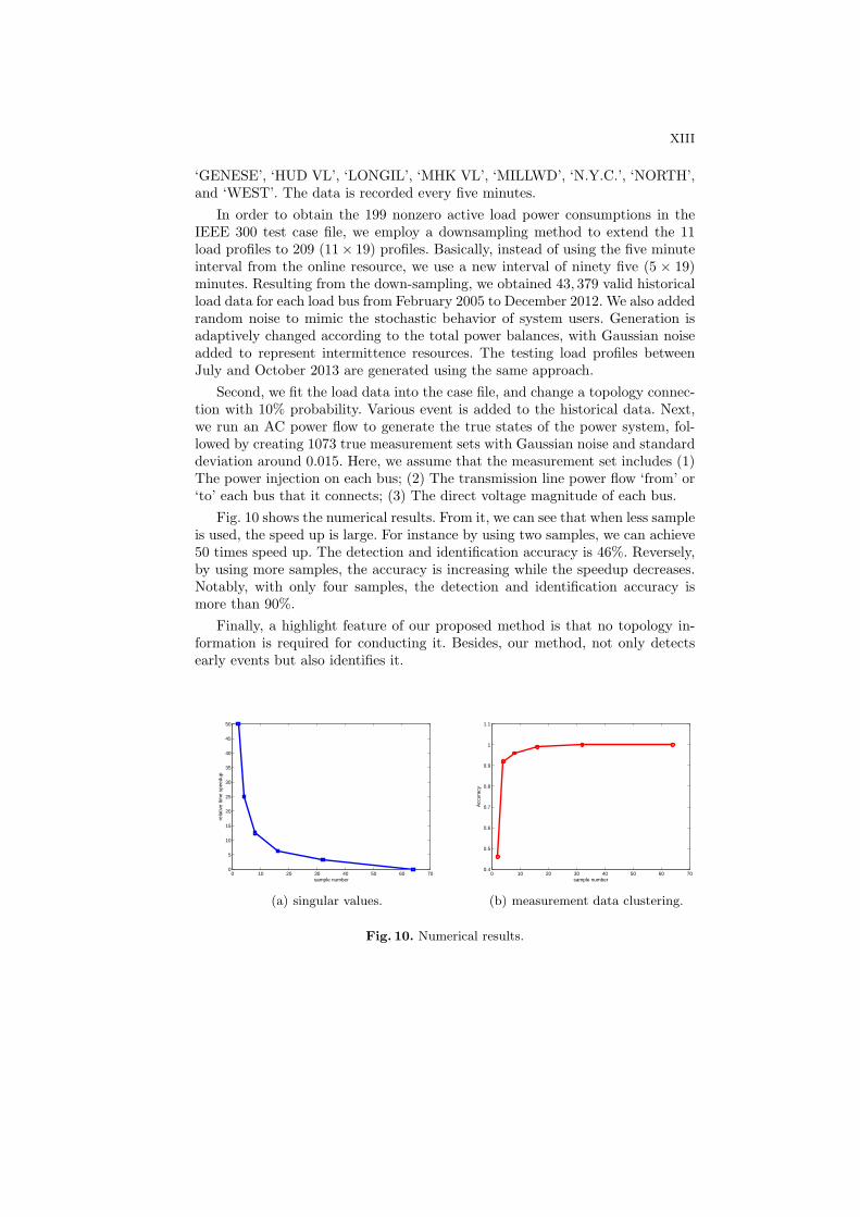
Fig. 10 shows the numerical results. From it, we can see that when less sampleis used, the speed up is large. For instance by using two samples, we can achieve50 times speed up. The detection and identification accuracy is 46%. Reversely,by using more samples, the accuracy is increasing while the speedup decreases.Notably, with only four samples, the detection and identification accuracy ismore than 90%.

Finally, a highlight feature of our proposed method is that no topology in-formation is required for conducting it. Besides, our method, not only detectsearly events but also identifies it.

0 10 20 30 40 50 60 700

5

10

15

20

25

30

35

40

45

50

sample number

rela

tive

time

spee

dup

(a) singular values.

0 10 20 30 40 50 60 700.4

0.5

0.6

0.7

0.8

0.9

1

1.1

sample number

Acc

urac

y

(b) measurement data clustering.

Fig. 10. Numerical results.

XIV

6 Conclusion

The challenges of smart gird are enormous as the power industry paradigm shift-s from the traditionally complex physical model based monitoring architectureto data-driven model based resource management. In this paper, we propose anew historical data-driven early event detection method based on data analysis.In particular, we conduct Singular Value Decomposition and Independent Com-ponent Analysis for power grid data. Subsequently, we propose an early eventdetection and identification approach on the basis of nearest sub-sequence searchand kernel regression model. This is based on the intuition that similar measure-ment sequences reflect similar power system events. Therefore, our data-drivenmethod is a unique way for sustainable smart grid design to break the currentmodel based monitoring architecture that requires both large complex modelingand computation overhead.

References

1. M. J. Smith and K. Wedeward, “Event detection and location in electric power sys-tems using constrained optimization,” Power and Energy Society General Meeting,pp. 26–30, Jul. 2009.

2. A. Abur and A. G. Exposito, “Power system state estimation: Theory and imple-mentation,” CRC Press, Mar. 2004.

3. B. C. Lesieutre, A. Pinar, and S. Roy, “Power system extreme event detection:The vulnerability frontier,” Proceedings of the 41st Annual Hawaii InternationalConference on System Sciences, p. 184, Jan. 2008.

4. L. D. Alvaro, “Development of distribution state estimation algorithms and appli-cation,” IEEE PES ISGT Europe, Oct. 2012.

5. J. Zhang, G. Welch, and G. Bishop, “Lodim: A novel power system state estimationmethod with dynamic measurement selection,” IEEE Power and Energy SocietyGeneral Meeting, Jul. 2011.

6. EATON, “Power xpert meters 4000/6000/8000.”7. M. Ilic, “Data-driven sustainable energy systems,” The 8th Annual Carnegie Mel-

lon Conference on the Elctricity industry, Mar. 2012.8. C. Yang, L. Xie, and P. R. Kumar, “Dimensionality reduction and early event

detection using online synchrophasor data,” Power and Energy Society GeneralMeeting, pp. 21–25, Jul. 2013.

9. C. M. Bishop, “Pattern recognition and machine learning,” Springer, 2006.10. G. Strang, “Introduction to linear algebra (section 6.7),” Wellesley-Cambridge

Press, 1998.11. Wikipedia, “Independent component analysis,” Apr. 2014.12. A. Hyvarinen, “Fastica for matlab,” http://research.ics.aalto.fi/ica/fastica/.13. R. D. Zimmerman, C. E. Murillo-Sanchez, , and R. J. Thomas, “Matpower’s exten-

sible optimal power flow architecture,” IEEE Power and Energy Society GeneralMeeting, pp. 1–7, Jul. 2009.

14. R. D. Zimmerman and C. E. Murillo-Sanchez, “Matpower, a matlab powersystem simulation package,” http://www.pserc.cornell.edu/ matpower/manual.pdf,Jul. 2010.

15. NYISO, “Load data profile,” http://www.nyiso.com, May. 2012.