Embed Size (px)
DESCRIPTION
POWER SYSTEM
Citation preview

Mathematics and Engineering Fundamentals 25
1 MATHEMATICS AND ENGINEERING FUNDAMENTALS
ENGINEERING METHODOLOGY
Engineering design is a process. As with many other processes, following the steps of the process provides no guarantee against failure but does enhance the chance of success. Each specific design application will have unique features thus requiring additional engineering in every application. Feedback in the design process takes into account that requirements can change or become more complicated. The design process should result in a system that meets all the requirements and specifications. The quality of the end product can be no better than the accuracy and completeness of the specifications.
Problem definition
Because problems are usually more complex than they seem, defining the problem to be solved by a design can be more difficult than developing the solution. The list of issues the solution system is to address and issues it is not to address is based on this definition. The problem can initially seem to be simple, such as the tripping of a home circuit breaker. But there can be many reasons for a circuit breaker to trip. Was the circuit breaker defective or did it trip to protect the circuit from an overloaded condition? Was there too much current for the circuit rating? Is the wiring faulty? Each of these reasons requires a different solution. None of them would have been resolved by simply resetting the circuit breaker.
Of course, the more complex the problem, the more effort is required to flush out the range of appropriate solutions. Be careful not to rush to a solution that solves either the wrong problem or a nonexistent problem. A thorough, accurate definition of the problem is the most important part of engineering design. The challenge in this phase is determining when you have collected adequate information to lead to a viable and economical solution.
System specifications
System specifications are measurable characteristics that describe the behavior of a system or action that solves the problem identified in the above engineering phase. Specifications constrain the solution to having a finite set of characteristics. Some of these characteristics have ranges of acceptable operation while others have exact attributes. Specifications are the targets that the solution must shoot for.
Specifications have a secondary function of validation. During subsequent design activities, the proposed solution must be tested for compliance to the specifications. If the problem definition phase was correctly completed and the proper specifications generated, the problem will be solved if and only if the solution system meets all the specifications.
Solution proliferation
Only very simple problems have obvious very best solutions. All other problems require a methodical search for possible solutions. At this point in the design phase, gather as many possible solutions as can be found. A fundamental rule is: the higher the number of identified potential solutions, the greater the chance of finding the optimal solution.

Mathematics and Engineering Fundamentals 25
Solution selection
There will probably be many good potential solutions but few, if any, that exactly meet the requirements. Create a weighted matrix to rank the usefulness of each solution. List all specifications in the right hand column of the matrix and the various design approaches across the top. Then assign a subjective weighting or multiplier to each specification, giving the highest weight to the most critical specifications. Enter the product of the specification weight and the degree to which the design approach meets that specification for each element under the different approaches. The sum of the column with the highest total is the favored approach for the problem under the given constraints.
If the chosen solution does not meet all the specifications, you may need to negotiate a compromise on the specifications or enhance the design approach (at some cost) to meet the requirements. If there are no suitable solutions, the choices are: look for more solutions, reevaluate the specifications, study the problem for ways to relax the specifications, or stop the design altogether because it is unfeasible. The first three alternatives represent the iterative nature of the design process. The fourth alternative, eliminating weak or unsuitable design approaches, has far fewer economic consequences at this point than later in the design cycle.
Design Implementation
So far, the process has only created a theoretical design and possibly some preliminary modeling or proof-of-concept studies to better qualify or rank the different approaches. The design implementation phase breaks the problem into manageable parts and assigns resources to the various parts. Such resources include engineering time, development tools, and of course, money. The process of developing many modules simultaneously is called concurrent engineering. A good approach to dividing the project up is to encapsulate it in such a way that each part can be tested separately from all others. The test plan should also ensure that minimal effort is needed to merge the various modules into the final system.
As testing and design progress, some modules may still not meet specifications. At this point, consider the same four alternatives that were discussed at the end of the previous section. Assuming all is progressing satisfactorily, testing processes and result documentation provide valuable and necessary information for validating redesigns and maintenance.
Final testing
A test plan should verify that the newly designed system meets all specifications. It is desirable that testing is time invariant, which means that once a system tests as valid, it is valid for all time. Software is time invariant. Excluding the software virus, any software bugs that show up after the equipment has spent time in the field were originally shipped in the new equipment. Hardware, however, is not time invariant since mechanical, thermal, and electrical stresses eventually wear out equipment.
Unfortunately, testing can only identify existing faults. It cannot verify the complete absence of faults. Power systems are far too complex to permit exhaustive testing from both a time and an economic perspective. A good test plan is fast and effective, providing repeatable expectation results. The bibliography at the end of this section lists references for additional information on developing approaches to testing and developing test plans.
Mathematics and Engineering Fundamentals 25
Documentation
Documentation is time consuming, but vital for good life cycle engineering. It covers test documents, manufacturing plans and instructions, patents, users’ manuals, field maintenance guides, application notes, and so on. These should be cross-referenced for easy information retrieval. Generating good documentation and maintaining documentation to track revisions requires meticulous attention but can be invaluable.
Installation and Commissioning
Good designs have thorough documentation and unambiguous labeling to minimize the chances of improper installation. Following well-documented procedures ensures nothing is forgotten. The less complicated the interface, the lower the risk of improper installation. Employing multiple levels of inspection also helps ensure proper installation and minimize potential damage to equipment.
Continuity, voltage profiles, and input-output actions tests are examples of multiple levels of inspection. The continuity test uses an ohmmeter to verify that equipment inputs and outputs have low resistance connections to the proper locations. Add to the thoroughness of the inspection by using a highlighter to identify circuits that have been checked. Correct any errors found before proceeding with the inspection. Once the continuity inspection is completed, you can energize the system. A good test procedure identifies voltages or currents at key locations. A chart is a good checklist for this inspection. Finally, applying known inputs and verifying the operations for proper response or outputs verifies system functionality.
BASIC ELECTRICAL SYSTEMS THEORY
Signal Representations
We can observe any signal from a perspective that focuses on the characteristics that have the greatest interest to us. Fourier analysis shows that we can represent any periodic waveform as the superposition sum of pure sine waves of different amplitudes and phases for the fundamental and harmonics. We can do the same for a periodic signal if we assume that the signal is periodic over the interval of observation. The four domains discussed below demonstrate how each domain presents pertinent data.
Time Domain
Equation 2.1 is the mathematical representation for a single frequency sinusoidal signal. The four dimensions of freedom are amplitude, frequency, phase, and time. You must know all four variables to determine the explicate value x(t) at any point in time. Complex signals may have mathematical representations that are too complicated to be meaningful just from observation. We frequently use time domain analysis to observe peak amplitude and/or timing relationships on an oscilloscope.
)2sin()( ϕπ +⋅⋅⋅⋅= tfAmtx Equation 2.1
Mathematics and Engineering Fundamentals 25
Frequency Domain – Fourier Series Analysis
Consider the time domain representation of a square wave as represented by Equation 2.2. We know from Fourier analysis that we can represent such a signal as a sum of sine and cosine function of varying amplitudes and at integer multiples of the fundamental frequency. Recall that this frequency is the inverse of the square wave period, T. Equation 2.3 shows the expression representing any periodic signal.
The terms cos(n ω0 t) and sin(n ω0 t) in Equation 2.3 describe fixed frequency sinusoidal signals that are common to all periodic signals. The only variables that depend strictly upon the characteristics of the signal under investigation are the coefficients B1n and B2n. The magnitude and phase of the nth harmonic of time domain signal x(t) are expressed by Equation 2.4 and Equation 2.5, respectively. The first harmonic is called the fundamental and the 0th harmonic is the dc component. This mechanism of separating one particular frequency from a group of frequencies is fundamental to power system protection using the magnitude and phase relationships of voltages and currents.
)mt(uAm)nt(uAm)t(x τ⋅−⋅−τ⋅−⋅= Equation 2.2
for n = 0, 2, 4, 6, …. And m = 1, 3, 5, 7, …
∑∑∞
=
∞
=
ω⋅⋅+ω⋅⋅=1k
0k00i
i )tksin(m2Bj)ticos(1B)t(x Equation 2.3
where ω0 = 2 π/T
2n
2n0 2B1B)n(Xm +=ω Equation 2.4
=ω
n
n0 2B
1Barctan)n(Xp Equation 2.5
Fourier analysis is a whole topic in itself; many good college texts cover the subject thoroughly.
Phase Domain
In the phase domain, the fundamental frequency is assumed to be fixed and time, other than for establishing a reference point, is inconsequential. Therefore the characteristics of a signal represented by Equation 2.1 can be expressed in the two remaining degrees of freedom, amplitude and phase. Equation 2.6 provides the same information as Equation 2.1 if the fundamental frequency, f, is known or is normalized to unity. Such representations are common in single frequency systems such as power systems. (See Bosela reference, Ch. 1, Pg. 13 i for additional information.)
ϕ∠= AmX Equation 2.6
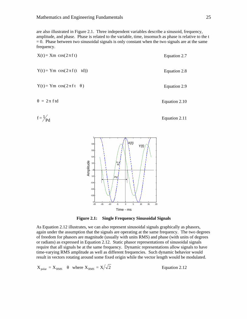
Phasors are normally used to represent a system of signals that operate at one frequency. Equation 2.7 through Equation 2.11 mathematically represents two such sinusoidal signals that
Mathematics and Engineering Fundamentals 25
are also illustrated in Figure 2.1. Three independent variables describe a sinusoid, frequency, amplitude, and phase. Phase is related to the variable, time, insomuch as phase is relative to the t = 0. Phase between two sinusoidal signals is only constant when the two signals are at the same frequency.
)tf2cos(Xm)t(X π⋅= Equation 2.7
))tdt(f2cos(Ym)t(Y +π⋅= Equation 2.8
) tf2cos(Ym)t(Y θ+π⋅= Equation 2.9
tdf2 π=θ Equation 2.10
Pd1f = Equation 2.11
-20 -15 -10 -5 0 5 10 15 20-1
-0.8
-0.6
-0.4
-0.2
0
0.2
0.4
0.6
0.8
1
td
X(t)Y(t)
Time - ms
Am
plitu
de
Pd
Figure 2.1: Single Frequency Sinusoidal Signals
As Equation 2.12 illustrates, we can also represent sinusoidal signals graphically as phasors, again under the assumption that the signals are operating at the same frequency. The two degrees of freedom for phasors are magnitude (usually with units RMS) and phase (with units of degrees or radians) as expressed in Equation 2.12. Static phasor representations of sinusoidal signals require that all signals be at the same frequency. Dynamic representations allow signals to have time-varying RMS amplitude as well as different frequencies. Such dynamic behavior would result in vectors rotating around some fixed origin while the vector length would be modulated.
2XXwhereXX RMSRMSpolar =θ∠= Equation 2.12
Mathematics and Engineering Fundamentals 25
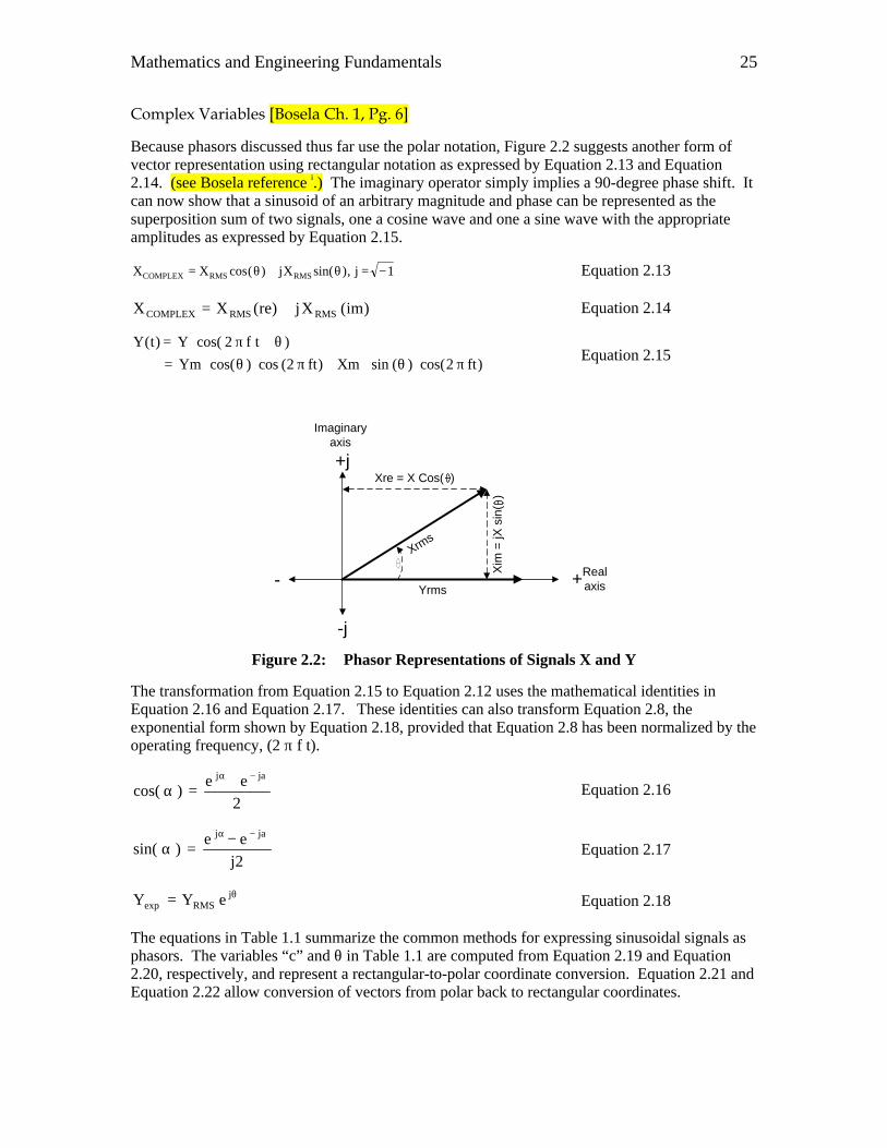
Complex Variables [Bosela Ch. 1, Pg. 6]
Because phasors discussed thus far use the polar notation, Figure 2.2 suggests another form of vector representation using rectangular notation as expressed by Equation 2.13 and Equation 2.14. (see Bosela reference i.) The imaginary operator simply implies a 90-degree phase shift. It can now show that a sinusoid of an arbitrary magnitude and phase can be represented as the superposition sum of two signals, one a cosine wave and one a sine wave with the appropriate amplitudes as expressed by Equation 2.15.
1j,)sin(Xj)(cosXX RMSRMSCOMPLEX −=θ+θ= Equation 2.13
)im(Xj)re(XX RMSRMSCOMPLEX += Equation 2.14
)ft2cos()(sinXm)ft2(cos)cos(Ym
) tf2cos(Y)t(Y
π⋅θ⋅+π⋅θ⋅=θ+π⋅=
Equation 2.15
Xrms
Xre = X Cos( )
Xim
= jX
sin
( )
Imaginaryaxis
Realaxis+
+j
-
-j
Yrms
Figure 2.2: Phasor Representations of Signals X and Y
The transformation from Equation 2.15 to Equation 2.12 uses the mathematical identities in Equation 2.16 and Equation 2.17. These identities can also transform Equation 2.8, the exponential form shown by Equation 2.18, provided that Equation 2.8 has been normalized by the operating frequency, (2 π f t).
2
ee)cos(
jaj −α +=α Equation 2.16
2j
ee)sin(
jaj −α −=α Equation 2.17
θ= jRMSexp eYY Equation 2.18
The equations in Table 1.1 summarize the common methods for expressing sinusoidal signals as phasors. The variables “c” and θ in Table 1.1 are computed from Equation 2.19 and Equation 2.20, respectively, and represent a rectangular-to-polar coordinate conversion. Equation 2.21 and Equation 2.22 allow conversion of vectors from polar back to rectangular coordinates.
Mathematics and Engineering Fundamentals 25
22|| bac += Equation 2.19
( )abarctan=θ Equation 2.20
)cos(|| θ⋅= ca Equation 2.21
Error! Objects cannot be created from editing field codes. Equation 2.22
Table 1.1: Phasor Form Identities
Rectangular Form
Complex Form
Exponential Form
Polar Form
Phasor Form
a + jb |c| •[ cos(θ) + jsin(θ) ] |c| ejθ |c| ∠θ c
a – jb |c| •[ cos(θ) – jsin(θ) ] |c| e-jθ |c| ∠-θ c*
-20 -15 -10 -5 0 5 10 15 20-0.8
-0.6
-0.4
-0.2
0
0.2
0.4
0.6
0.8
Y(t)=Yre(t)+Yim(t)
Yim(t)
Yre(t)Am
plitu
de
Time - ms
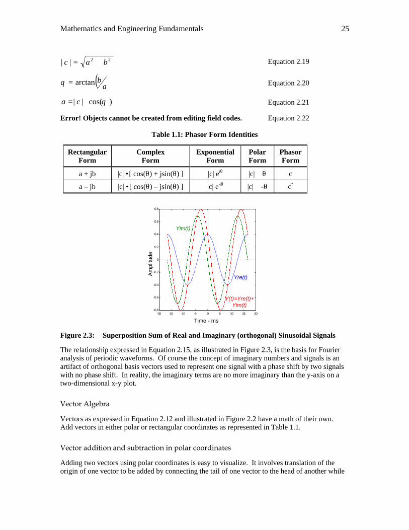
Figure 2.3: Superposition Sum of Real and Imaginary (orthogonal) Sinusoidal Signals
The relationship expressed in Equation 2.15, as illustrated in Figure 2.3, is the basis for Fourier analysis of periodic waveforms. Of course the concept of imaginary numbers and signals is an artifact of orthogonal basis vectors used to represent one signal with a phase shift by two signals with no phase shift. In reality, the imaginary terms are no more imaginary than the y-axis on a two-dimensional x-y plot.
Vector Algebra
Vectors as expressed in Equation 2.12 and illustrated in Figure 2.2 have a math of their own. Add vectors in either polar or rectangular coordinates as represented in Table 1.1.
Vector addition and subtraction in polar coordinates
Adding two vectors using polar coordinates is easy to visualize. It involves translation of the origin of one vector to be added by connecting the tail of one vector to the head of another while
Mathematics and Engineering Fundamentals 25
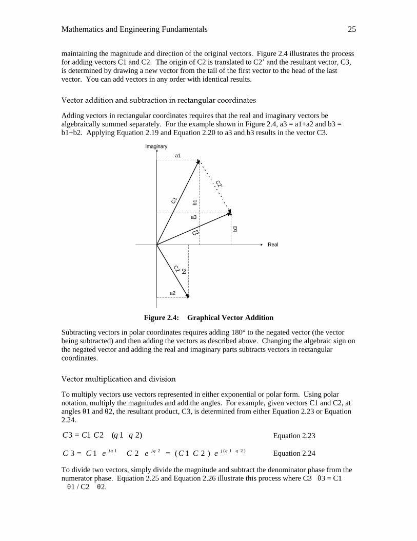
maintaining the magnitude and direction of the original vectors. Figure 2.4 illustrates the process for adding vectors C1 and C2. The origin of C2 is translated to C2’ and the resultant vector, C3, is determined by drawing a new vector from the tail of the first vector to the head of the last vector. You can add vectors in any order with identical results.
Vector addition and subtraction in rectangular coordinates
Adding vectors in rectangular coordinates requires that the real and imaginary vectors be algebraically summed separately. For the example shown in Figure 2.4, a3 = a1+a2 and b3 = b1+b2. Applying Equation 2.19 and Equation 2.20 to a3 and b3 results in the vector C3.
C1
C2'
C2
C3
Real
Imaginary
a1
b1
b2
a2
b3
a3
Figure 2.4: Graphical Vector Addition
Subtracting vectors in polar coordinates requires adding 180° to the negated vector (the vector being subtracted) and then adding the vectors as described above. Changing the algebraic sign on the negated vector and adding the real and imaginary parts subtracts vectors in rectangular coordinates.
Vector multiplication and division
To multiply vectors use vectors represented in either exponential or polar form. Using polar notation, multiply the magnitudes and add the angles. For example, given vectors C1 and C2, at angles θ1 and θ2, the resultant product, C3, is determined from either Equation 2.23 or Equation 2.24.
)21(213 θθ +∠⋅= CCC Equation 2.23
)21(21 )21(213 θθθθ +=⋅⋅⋅= jjj eCCeCeCC Equation 2.24
To divide two vectors, simply divide the magnitude and subtract the denominator phase from the numerator phase. Equation 2.25 and Equation 2.26 illustrate this process where C3∠θ3 = C1 ∠θ1 / C2 ∠θ2.
Mathematics and Engineering Fundamentals 25
( ) )21(213 θθ −∠= C
CC Equation 2.25
( ) ( ) )21(212
1
21
21
213 θθθθ
θ
θ−− =⋅⋅
=
⋅⋅= jjj
j
j
eCCeeC
CeC
eCC Equation 2.26
Per Unit Computations
For additional information, consult any quality text on the fundamentals of power system analysis. The reference for the companion Bosela text is Ch. 5, pg. 123-155. i,v, vi, x Appendix 11 also has a discussion of per-unit calculations.
Three Phase AC Theory
We are assuming that readers have a rudimentary knowledge of this subject. Refer to the companion text by Bosela Ch. 1, pg. 37-44 i for additional information.
Transmission Line Models
Transmission lines and distribution lines are in the strictest sense conductors of electrical energy. They consist of one or more energized lines and a neutral line. Utilities using multigrounded neutral systems tie the neutral wire to an earth ground at multiple places along the line length. Lines in general refer to bipolar and unipolar dc transmission lines, single and three phase ac overhead transmission and distribution lines, and single and multiphase underground cables.
The line model chosen to represent the characteristics of an electrical line depends on three factors: 1) the frequency range under consideration, 2) the degree of accuracy required, and 3) the available data on which to base the model. For background information on mathematical models of power lines, refer to the Bosela reference text.i
Single-Phase Representations
Single-phase models usually include the electrical characteristics of the supply conductor but rarely consider parameters associated with the return path. If return path considerations are included, they are generally included in the supply path. Splitting the line into a supply conductor and a return conductor usually requires a multiphase line model, as discussed in section 0.
LR Models
The most basic line models include approximations of the line self-impedance or positive-sequence impedance. Nominal values for common conductors are provided in numerous texts and wire vendor data sheets.i, ii Further simplifications are possible depending on the expected range of frequencies for signals that will be imposed on the line. If the source is dc, then consider only the resistive component of the line. For ac signals and dc signals including transient effects, consider both the resistance and inductance until either the reactive impedance is much greater than the resistance or the error introduced by ignoring the resistance is acceptable. LR models are also suitable for short (zero to 10 miles) single and multiphase bare overhead lines when they are modeled as three single-phase lines.
Mathematics and Engineering Fundamentals 25
LRC Lumped Parameter Pi Models
There are two different uses of the LRC transmission line models. The first use is for studying systems for steady-state phenomena only. It is then appropriate to use the LRC model regardless of line length. The LRC line model is also appropriate for modeling medium length (10-30 miles) bare overhead lines in transient studies. Only use single-phase LRC models to model single-phase lines.
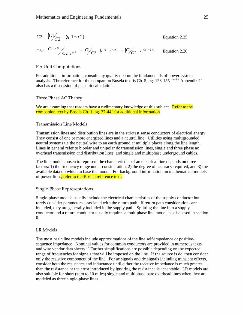
The nominal line-to-ground capacitance is usually evenly distributed between two capacitors that are placed next to the line terminals as shown in Figure 2.5.
Cs/2
LsRs
A ACs/2
Figure 2.5: Single-Phase Lumped-Parameter Line Model
Distributed Line Parameter
Electromagnetic Transient Program (EMTP) studies use distributed parameter line models for modeling bare overhead lines longer than 30 miles. The chief characteristics of this model are the characteristic impedance and the propagation time. When dealing with long lines, remember that the effects of transient reflections and Ferranti voltage rise occur frequently on long, improperly terminated transmission lines.
This line model is appropriate for modeling single-phase or single-phase representations of balanced three-phase lines that have low losses (the resistance is small relative to the reactive impedance of the lowest signal frequency).
There are one-to-one correlations between the line inductance and capacitance shown in Figure 2.5 and the characteristic impedance, Zc, and the travel time, τ. Equation 2.27 and Equation 2.28 express the relationships for the lossless line models. If Ls and Cs in these equations have units per unit length, then the total travel time is determined by multiplying by the line length. Losses can be included by modifying Zc computed in Equation 2.27 to be Zc’ computed by Equation 2.29.
Cs
LsZc = Equation 2.27
CsLs=τ Equation 2.28
Cs
RsZcZc
+=' Equation 2.29
Frequently the characteristic impedance is also called the surge impedance. This impedance is real in value, rather than complex. It is the impedance of the transmission line and does not include the terminating impedances at the opposite ends of the line. If the transmission line is not
Mathematics and Engineering Fundamentals 25
terminated into its characteristic impedance, then the mismatched impedance generates reflections.
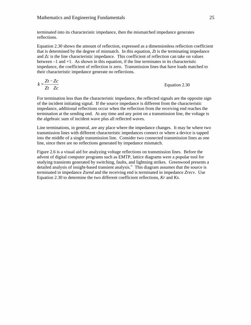
Equation 2.30 shows the amount of reflection, expressed as a dimensionless reflection coefficient that is determined by the degree of mismatch. In this equation, Zt is the terminating impedance and Zc is the line characteristic impedance. This coefficient of reflection can take on values between –1 and +1. As shown in this equation, if the line terminates in its characteristic impedance, the coefficient of reflection is zero. Transmission lines that have loads matched to their characteristic impedance generate no reflections.
ZcZt
ZcZtk
+−
= Equation 2.30
For termination less than the characteristic impedance, the reflected signals are the opposite sign of the incident initiating signal. If the source impedance is different from the characteristic impedance, additional reflections occur when the reflection from the receiving end reaches the termination at the sending end. At any time and any point on a transmission line, the voltage is the algebraic sum of incident wave plus all reflected waves.
Line terminations, in general, are any place where the impedance changes. It may be where two transmission lines with different characteristic impedances connect or where a device is tapped into the middle of a single transmission line. Consider two connected transmission lines as one line, since there are no reflections generated by impedance mismatch.
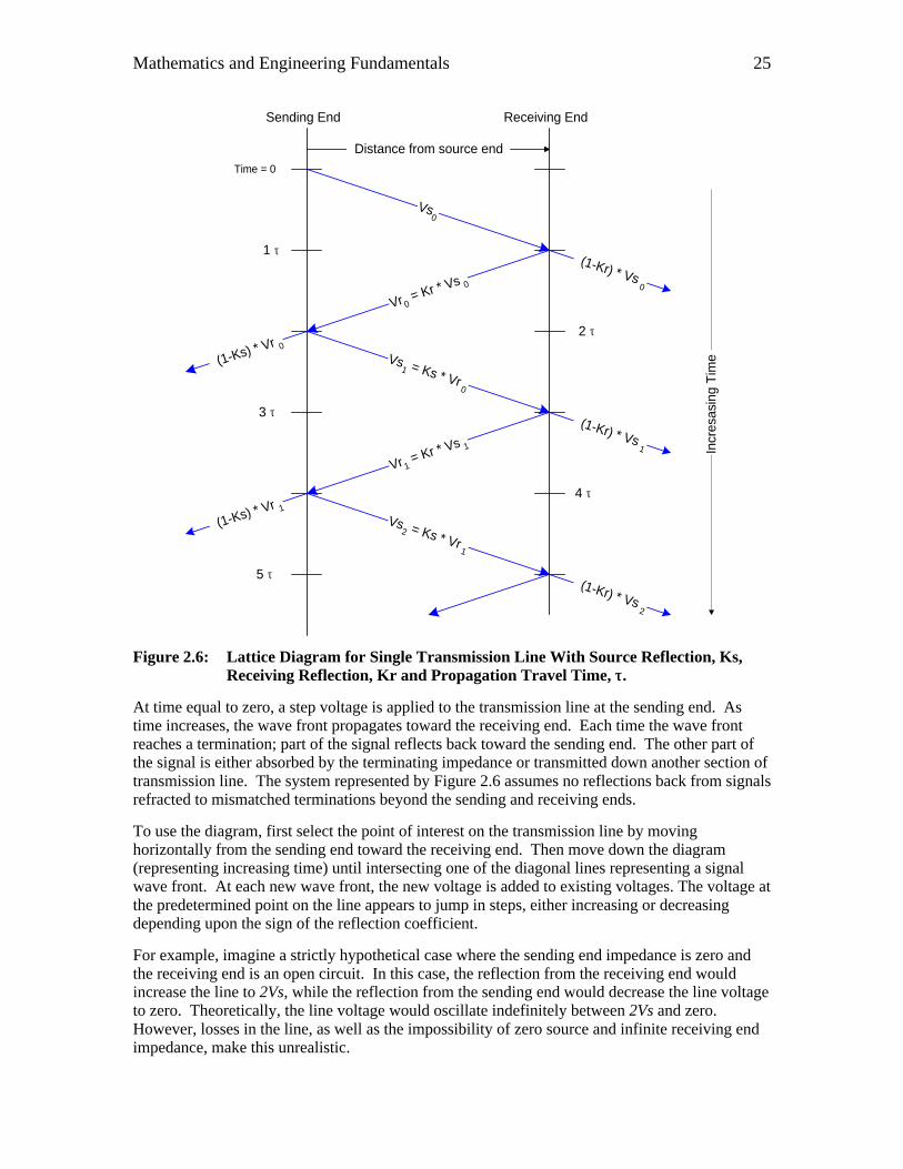
Figure 2.6 is a visual aid for analyzing voltage reflections on transmission lines. Before the advent of digital computer programs such as EMTP, lattice diagrams were a popular tool for studying transients generated by switching, faults, and lightning strikes. Greenwood presents a detailed analysis of insight-based transient analysis.iii This diagram assumes that the source is terminated in impedance Zsend and the receiving end is terminated in impedance Zrecv. Use Equation 2.30 to determine the two different coefficient reflections, Kr and Ks.
Mathematics and Engineering Fundamentals 25
Vs0
Vr 0 = Kr * V
s 0
Vs1 = Ks * Vr
0
Vr 1 = Kr * V
s 1
Vs2 = Ks * Vr
1
Sending End Receiving End
(1-Kr) * Vs0
(1-Ks) * Vr 0
(1-Kr) * Vs1
(1-Ks) * Vr 1
(1-Kr) * Vs2
Time = 0
1 τ
2 τ
4 τ
3 τ
5 τ
Distance from source end
Incr
esas
ing
Tim
e
Figure 2.6: Lattice Diagram for Single Transmission Line With Source Reflection, Ks, Receiving Reflection, Kr and Propagation Travel Time, ττ.
At time equal to zero, a step voltage is applied to the transmission line at the sending end. As time increases, the wave front propagates toward the receiving end. Each time the wave front reaches a termination; part of the signal reflects back toward the sending end. The other part of the signal is either absorbed by the terminating impedance or transmitted down another section of transmission line. The system represented by Figure 2.6 assumes no reflections back from signals refracted to mismatched terminations beyond the sending and receiving ends.
To use the diagram, first select the point of interest on the transmission line by moving horizontally from the sending end toward the receiving end. Then move down the diagram (representing increasing time) until intersecting one of the diagonal lines representing a signal wave front. At each new wave front, the new voltage is added to existing voltages. The voltage at the predetermined point on the line appears to jump in steps, either increasing or decreasing depending upon the sign of the reflection coefficient.
For example, imagine a strictly hypothetical case where the sending end impedance is zero and the receiving end is an open circuit. In this case, the reflection from the receiving end would increase the line to 2Vs, while the reflection from the sending end would decrease the line voltage to zero. Theoretically, the line voltage would oscillate indefinitely between 2Vs and zero. However, losses in the line, as well as the impossibility of zero source and infinite receiving end impedance, make this unrealistic.
Mathematics and Engineering Fundamentals 25
Losses can be included into this model by computing a loss reflection coefficient, Kloss, based on a new characteristic impedance determined from Equation Error! Reference source not found.. Subsequently, the new coefficients for the model presented in Figure 2.6 are represented by Ks’ and Kr’ from Equations Equation 2.31) through Equation 2.33), below. For finite Rs, Kloss is always less than unity and the reflections will eventually decay to zero.
ZcZc
ZcZcKloss
+−
='
' Equation 2.31
KlossKsKs ⋅=' Equation 2.32
KlossKrKr ⋅=' Equation 2.33
It is easy to imagine the difficulty of modeling multiple transmission lines with differing travel times and characteristic impedances. Such intuitions are very useful if not absolutely necessary when validating EMTP models. EMTP is invaluable for developing a sense of what kind of voltage and current transients might be generated by a lightning surge as it propagates down a transmission line into a substation. This tool is also good for developing intuitions about transient behavior.
Because lattice diagrams are strictly a time domain tool, inductive and capacitive terminations give rise to exponential responses. Capacitive terminations change with time from short circuits to open circuits as the capacitor charges. Inductive terminations change from open circuits to short circuits. Termination in either device results in time-varying coefficients of reflection.
Multiphase Lumped Parameter Line Models
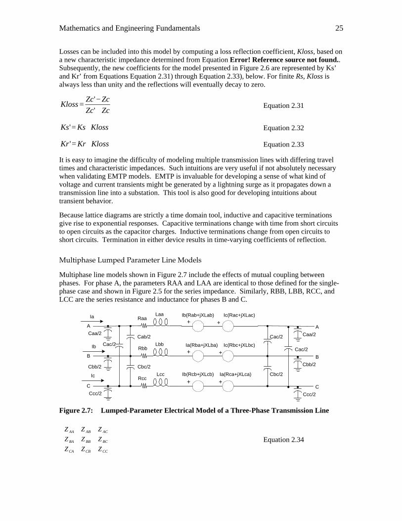
Multiphase line models shown in Figure 2.7 include the effects of mutual coupling between phases. For phase A, the parameters RAA and LAA are identical to those defined for the single-phase case and shown in Figure 2.5 for the series impedance. Similarly, RBB, LBB, RCC, and LCC are the series resistance and inductance for phases B and C.
Caa/2Cac/2
Cac/2
Cbc/2
Laa
Lbb
Lcc
Raa
Rbb
Rcc
A A
B B
C C
Cbb/2
Ccc/2
Caa/2
Cbb/2
Ccc/2
Cab/2
Cac/2
Cbc/2
Ib(Rab+jXLab)Ia
Ib
Ic
+ +
+ +
+ +
Ic(Rac+jXLac)
Ib(Rcb+jXLcb) Ia(Rca+jXLca)
Ic(Rbc+jXLbc)Ia(Rba+jXLba)
Figure 2.7: Lumped-Parameter Electrical Model of a Three-Phase Transmission Line
CCCBCA
BCBBBA
ACABAA
ZZZ
ZZZ
ZZZ Equation 2.34
Mathematics and Engineering Fundamentals 25
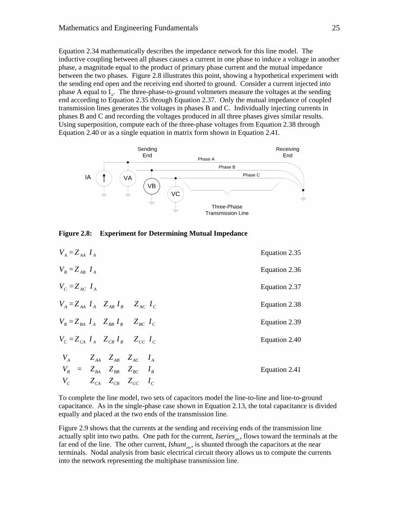
Equation 2.34 mathematically describes the impedance network for this line model. The inductive coupling between all phases causes a current in one phase to induce a voltage in another phase, a magnitude equal to the product of primary phase current and the mutual impedance between the two phases. Figure 2.8 illustrates this point, showing a hypothetical experiment with the sending end open and the receiving end shorted to ground. Consider a current injected into phase A equal to IA. The three-phase-to-ground voltmeters measure the voltages at the sending end according to Equation 2.35 through Equation 2.37. Only the mutual impedance of coupled transmission lines generates the voltages in phases B and C. Individually injecting currents in phases B and C and recording the voltages produced in all three phases gives similar results. Using superposition, compute each of the three-phase voltages from Equation 2.38 through Equation 2.40 or as a single equation in matrix form shown in Equation 2.41.
VAIAVB
VC
Three-PhaseTransmission Line
Phase A
Phase B
Phase C
SendingEnd
ReceivingEnd
Figure 2.8: Experiment for Determining Mutual Impedance
AAAA IZV = Equation 2.35
AABB IZV = Equation 2.36
AACC IZV = Equation 2.37
CACBABAAAA IZIZIZV ++= Equation 2.38
CBCBBBABAB IZIZIZV ++= Equation 2.39
CCCBCBACAC IZIZIZV ++= Equation 2.40
=
C
B
A
CCCBCA
BCBBBA
ACABAA
C
B
A
I
I
I
ZZZ
ZZZ
ZZZ
V
V
V
Equation 2.41
To complete the line model, two sets of capacitors model the line-to-line and line-to-ground capacitance. As in the single-phase case shown in Equation 2.13, the total capacitance is divided equally and placed at the two ends of the transmission line.
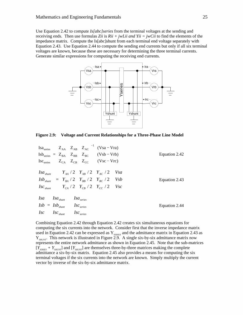
Figure 2.9 shows that the currents at the sending and receiving ends of the transmission line actually split into two paths. One path for the current, Iseriesabc, flows toward the terminals at the far end of the line. The other current, Ishuntabc, is shunted through the capacitors at the near terminals. Nodal analysis from basic electrical circuit theory allows us to compute the currents into the network representing the multiphase transmission line.
Mathematics and Engineering Fundamentals 25
Use Equation 2.42 to compute Is[abc]series from the terminal voltages at the sending and receiving ends. Then use formulas Zii is Rii + jωLii and Yii = jωCii to find the elements of the impedance matrix. Compute the Is[abc]shunt from each terminal end voltage separately with Equation 2.43. Use Equation 2.44 to compute the sending end currents but only if all six terminal voltages are known, because these are necessary for determining the three terminal currents. Generate similar expressions for computing the receiving end currents.
Vsa
Vsb
Vsc
Vra
Vrb
Vrc
Isa
Isb
Isc
Ira
Irb
Irc
Yse
ries
Yshunt Yshunt
Figure 2.9: Voltage and Current Relationships for a Three-Phase Line Model
−−−
=
−
)VrcVsc(
)VrbVsb(
)VraVsa(
ZZZ
ZZZ
ZZZ
Isc
Isb
Isa1
CCCBCA
BCBBBA
ACABAA
series
series
series
Equation 2.42
=
Vsc
Vsb
Vsa
YYY
YYY
YYY
Isc
Isb
Isa
CCCBCA
BCBBBA
ACABAA
shunt
shunt
shunt
2/2/2/
2/2/2/
2/2/2/
Equation 2.43
+
=
series
series
series
shunt
shunt
shunt
Isc
Isc
Isa
Isc
Isb
Isa
Isc
Isb
Isa
Equation 2.44
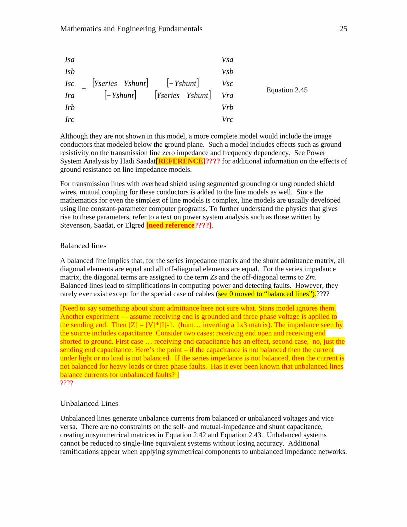
Combining Equation 2.42 through Equation 2.42 creates six simultaneous equations for computing the six currents into the network. Consider first that the inverse impedance matrix used in Equation 2.42 can be expressed as YSERIES and the admittance matrix in Equation 2.43 as YSHUNT. This network is illustrated in Figure 2.9. A single six-by-six admittance matrix now represents the entire network admittance as shown in Equation 2.45. Note that the sub-matrices [YSERIES + YSHUNT] and [YSHUNT] are themselves three-by-three matrices making the complete admittance a six-by-six matrix. Equation 2.45 also provides a means for computing the six terminal voltages if the six currents into the network are known. Simply multiply the current vector by inverse of the six-by-six admittance matrix.
Mathematics and Engineering Fundamentals 25
[ ] [ ][ ] [ ]
+−
−+=
Vrc
Vrb
Vra
Vsc
Vsb
Vsa
YshuntYseriesYshunt
YshuntYshuntYseries
Irc
Irb
Ira
Isc
Isb
Isa
Equation 2.45
Although they are not shown in this model, a more complete model would include the image conductors that modeled below the ground plane. Such a model includes effects such as ground resistivity on the transmission line zero impedance and frequency dependency. See Power System Analysis by Hadi Saadat[REFERENCE]???? for additional information on the effects of ground resistance on line impedance models.
For transmission lines with overhead shield using segmented grounding or ungrounded shield wires, mutual coupling for these conductors is added to the line models as well. Since the mathematics for even the simplest of line models is complex, line models are usually developed using line constant-parameter computer programs. To further understand the physics that gives rise to these parameters, refer to a text on power system analysis such as those written by Stevenson, Saadat, or Elgred [need reference????].
Balanced lines
A balanced line implies that, for the series impedance matrix and the shunt admittance matrix, all diagonal elements are equal and all off-diagonal elements are equal. For the series impedance matrix, the diagonal terms are assigned to the term Zs and the off-diagonal terms to Zm. Balanced lines lead to simplifications in computing power and detecting faults. However, they rarely ever exist except for the special case of cables (see 0 moved to “balanced lines”).????
[Need to say something about shunt admittance here not sure what. Stans model ignores them. Another experiment --- assume receiving end is grounded and three phase voltage is applied to the sending end. Then [Z] = [V]*[I]-1. (hum… inverting a 1x3 matrix). The impedance seen by the source includes capacitance. Consider two cases: receiving end open and receiving end shorted to ground. First case … receiving end capacitance has an effect, second case, no, just the sending end capacitance. Here’s the point – if the capacitance is not balanced then the current under light or no load is not balanced. If the series impedance is not balanced, then the current is not balanced for heavy loads or three phase faults. Has it ever been known that unbalanced lines balance currents for unbalanced faults? ] ????
Unbalanced Lines
Unbalanced lines generate unbalance currents from balanced or unbalanced voltages and vice versa. There are no constraints on the self- and mutual-impedance and shunt capacitance, creating unsymmetrical matrices in Equation 2.42 and Equation 2.43. Unbalanced systems cannot be reduced to single-line equivalent systems without losing accuracy. Additional ramifications appear when applying symmetrical components to unbalanced impedance networks.
Mathematics and Engineering Fundamentals 25
Multiphase Distributed Line Parameter Models
Multiphase distributed line modes extend the basic model presented in 0. However, they require a transformation to generate an orthogonal set of equations that allows the three-phase transmission line to be represented by three single-phase lines. The symmetrical components discussion in 0 includes the mathematics for the base transformation. The multiphase distributed line parameter model is valid only if the matrix equations can be transformed to an orthogonal basis vector using a similarity transformation, to be discussed next. Once this is accomplished, the multiphase transmission lines can be represented as multiple independent single-phase lines. This results in no coupling between phases in the transformed mode.
Balanced Lines in Distributed Line Parameter Models
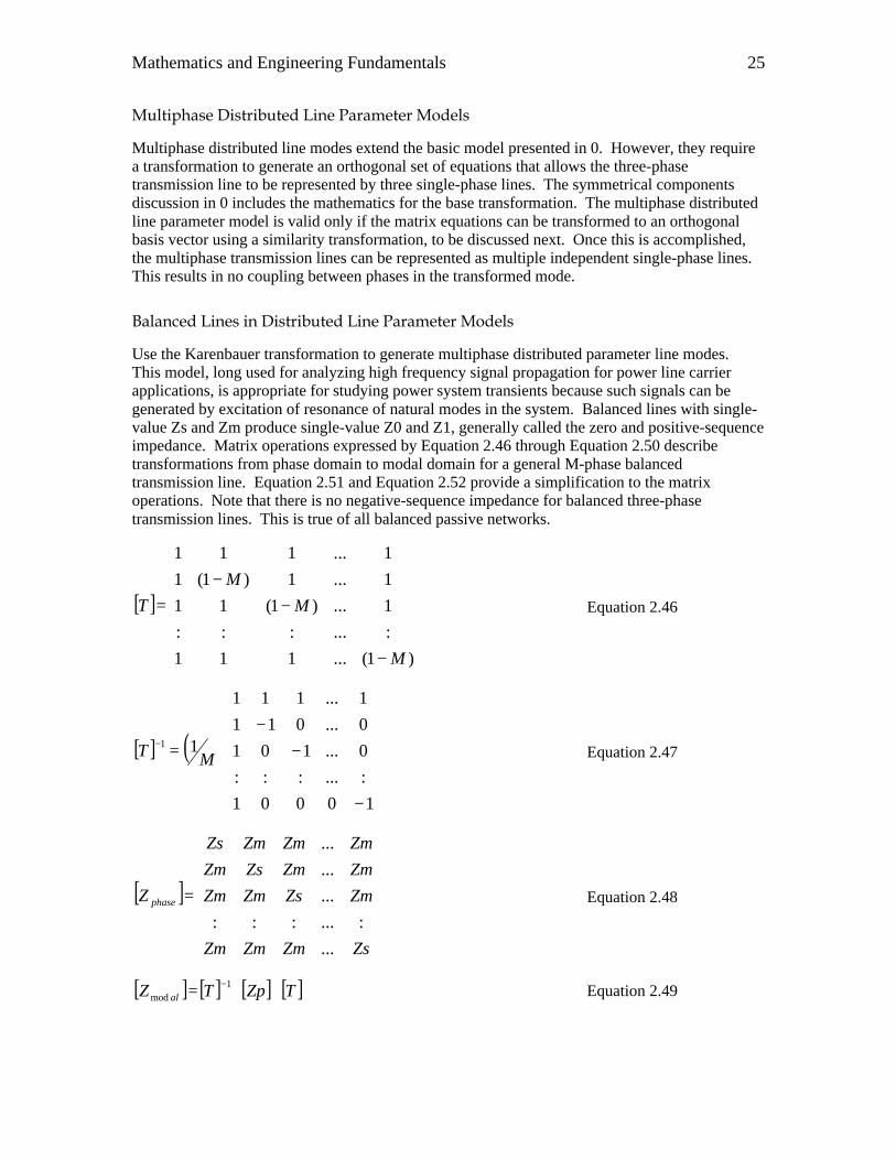
Use the Karenbauer transformation to generate multiphase distributed parameter line modes. This model, long used for analyzing high frequency signal propagation for power line carrier applications, is appropriate for studying power system transients because such signals can be generated by excitation of resonance of natural modes in the system. Balanced lines with single-value Zs and Zm produce single-value Z0 and Z1, generally called the zero and positive-sequence impedance. Matrix operations expressed by Equation 2.46 through Equation 2.50 describe transformations from phase domain to modal domain for a general M-phase balanced transmission line. Equation 2.51 and Equation 2.52 provide a simplification to the matrix operations. Note that there is no negative-sequence impedance for balanced three-phase transmission lines. This is true of all balanced passive networks.
[ ]
−
−−
=
)1(...111
:...:::
1...)1(11
1...1)1(1
1...111
M
M
M
T Equation 2.46
[ ] ( )
−
−−
=−
10001
:...:::
0...101
0...011
1...111
11
MT Equation 2.47
[ ]
=
ZsZmZmZm
ZmZsZmZm
ZmZmZsZm
ZmZmZmZs
Z phase
...
:...:::
...
...
...
Equation 2.48
[ ] [ ] [ ] [ ]TZpTZ al1
mod−= Equation 2.49
Mathematics and Engineering Fundamentals 25
[ ]
=
1...000
:...:::
0...100
0...10
0...000
mod
Z
Z
Z
Z
Z al Equation 2.50
)LmjRm)(1M()LsjRs(
0Lj0RZm)1M(Zs0Z
ω+−+ω=ω+=⋅−+=
Equation 2.51
)(1 LmjRmLsjRsZmZsZ ωω +−+=−= Equation 2.52
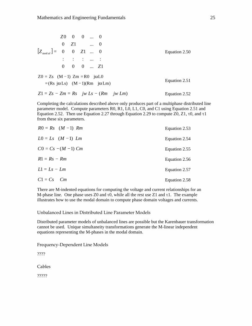
Completing the calculations described above only produces part of a multiphase distributed line parameter model. Compute parameters R0, R1, L0, L1, C0, and C1 using Equation 2.51 and Equation 2.52. Then use Equation 2.27 through Equation 2.29 to compute Z0, Z1, τ0, and τ1 from these six parameters.
RmMRsR )1(0 −+= Equation 2.53
LmMLsL )1(0 −+= Equation 2.54
CmMCsC )1(0 −−= Equation 2.55
RmRsR −=1 Equation 2.56
LmLsL −=1 Equation 2.57
CmCsC +=1 Equation 2.58
There are M-indented equations for computing the voltage and current relationships for an M-phase line. One phase uses Z0 and τ0, while all the rest use Z1 and τ1. The example illustrates how to use the modal domain to compute phase domain voltages and currents.
Unbalanced Lines in Distributed Line Parameter Models
Distributed parameter models of unbalanced lines are possible but the Karenbauer transformation cannot be used. Unique simultaneity transformations generate the M-linear independent equations representing the M-phases in the modal domain.
Frequency-Dependent Line Models
????
Cables
?????
Mathematics and Engineering Fundamentals 25
Domain Transformations
The subject working in companion domains has already been introduced, as the Karenbauer transformation that is needed for modeling distributed line parameter models using the modal domain. As mentioned before, this is one of many transformations into a domain that results in an impedance matrix that has all zero off-diagonal elements. The value of such transformations is that independent equations can be used to solve for voltages and currents that have coupled three-phase impedance relationships. The disadvantage is that one must be able to interpret the results obtained in the uncoupled domain or easily convert back to the phase domain.
Symmetrical Components [6066], [Bosela Ch. 10, Pg. 332-370]
Fortescue first introduced symmetrical components in 1918. He demonstrated that an M-phase unbalance system can be represented as M-1 M-phase systems of differing orders of sequences and one zero phase sequence. A thorough treatment on the subject of symmetrical components is provided in a text written by Dr. Paul Anderson.iv Further treatment of this subject is provided in Appendix Error! Reference source not found. and in the tutorial written by Stan Zocholl.v
Although not strictly limited to three-phase networks, symmetrical components are frequently used to analyze conventional three-phase power systems. To illustrate, consider a three-phase unbalanced system denoted as phases A, B, and C. We introduce a phase-shifting operator, “a” such that a phasor aV∠θ° = V∠(θ+φ)° and for this example, φ equal 120°. Raising α to a power is equivalent to multiplying 120° by that number.
Equation 2.60 provides the transformation from the phase domain to the symmetrical component domain. The matrix shown in Equation 2.60 is called the Fortescue transformation matrix. It is convention to refer to phase A zero-sequence voltage as VA0, phase A positive-sequence voltage as VA1, and phase A negative-sequence impedance as VA2. The reference to phase A defines the rotational sequence for phase B and C such that the positive-sequence phasors align all three phases, A, B, and C, with phase A. It is sometimes convenient to assume phase A is the reference phase and therefore drop the reference to phase A notation. In such cases, the positive-, negative-, and zero-sequence voltages are the denoted by V1, V2, and V3 respectively. Equation 2.60 through Equation 2.62 express the same information as Equation 2.59 but as three independent equations. Use similar expressions for current.
( ) [ ] [ ] [ ]ABC
C
B
A
A
A
A
VAVor
V
V
V
aa
aa
V
V
V
⋅=
⋅
=
012
2
2
1
1
111
31
2
1
0
Equation 2.59
3/)(0 CCBBAAA VVVV θθθ ∠+∠+∠= Equation 2.60
3/)VVV(1V 2CC
1BB
0AAA α⋅θ∠+α⋅θ∠+α⋅θ∠= Equation 2.61
3/)(2 120 αθαθαθ ⋅∠+⋅∠+⋅∠= CCBBAAA VVVV Equation 2.62
Equation 2.63 or Equation 2.64 through Equation 2.66 provide the transformation from the symmetrical component domain back to the phase domain. As before, use similar expressions for current.
Mathematics and Engineering Fundamentals 25
[ ] [ ] [ ]0121
2
2
2
1
0
1
1
111
VAVor
V
V
V
aa
aa
V
V
V
ABC
A
A
A
C
B
A
⋅=
⋅
=
−
Equation 2.63
210 AAAA VVVVa ++=∠θ Equation 2.64
120 210 αααθ ⋅+⋅+⋅=∠ AAAB VVVVb Equation 2.65
210 210 αααθ ⋅+⋅+⋅=∠ AAAC VVVVc Equation 2.66
The line model developed in paragraph 0, and the impedance transformations shown in Equation 2.46 through Equation 2.58 are adequate for transforming impedance of balanced networks from the phase domain to the symmetrical component domain. The significance of working in the symmetrical component domain is that zero-sequence currents only generate zero-sequence voltages if the zero-sequence impedance is not zero. The same can be said for positive- and negative-sequence currents, voltages, and impedances. Equation 2.67 expresses this relationship mathematically. Since the impedances are uncoupled, we can write Equation 2.67 as three individual equations, as shown in Equation 2.68 through Equation 2.70.
[ ] [ ] [ ]012012012
2
1
0
200
010
000
2
1
0
IZVor
I
I
I
Z
Z
Z
V
V
V
A
A
A
A
A
A
⋅=
⋅
=
Equation 2.67
000 IZV ⋅= Equation 2.68
111 IZV ⋅= Equation 2.69
222 IZV ⋅= Equation 2.70
An impedance transformation from the phase domain to the sequence domain follows from extensions of Equation 2.59, Equation 2.63, and Equation 2.67. In symmetrical component domain and phase domain, express Ohm’s law as in Equation 2.67 and Equation 2.71, respectively. Substituting Equation 2.71 into Equation 2.59 yields Equation 2.72. The transformation of currents from the phase domain to the symmetrical component domain follows from Equation 2.63, as shown in Equation 2.73. Making the substitution for IABC from Equation 2.73 into Equation 2.72 expresses voltages and currents in the symmetrical component domain as a function of impedance in the phase domain shown in Equation 2.74. Compare Equation 2.67 and Equation 2.74 to deduce the relationship of symmetrical component impedance to phase domain impedance that is shown in Equation 2.75.
[ ] [ ] [ ]ABCABCABC IZV ⋅= Equation 2.71
[ ] [ ] [ ] [ ]ABCABC IZAV ⋅⋅=012 Equation 2.72
[ ] [ ] [ ]0121 IAI ABC ⋅= −
Equation 2.73
[ ] [ ] [ ] [ ] [ ]0121
012 IAZAV ABC ⋅⋅⋅= − Equation 2.74
Mathematics and Engineering Fundamentals 25
[ ] [ ] [ ] [ ] 1012
−⋅⋅= AZAZ ABC Equation 2.75
If phase domain impedance, ZABC, is generated for a balanced network, then the results from Equation 2.75 are identical to the results from Equation 2.51 and Equation 2.52 with the negative-sequence impedance set equal to the positive-sequence impedance. For balanced networks, all mutual- and all self-impedances are equal.
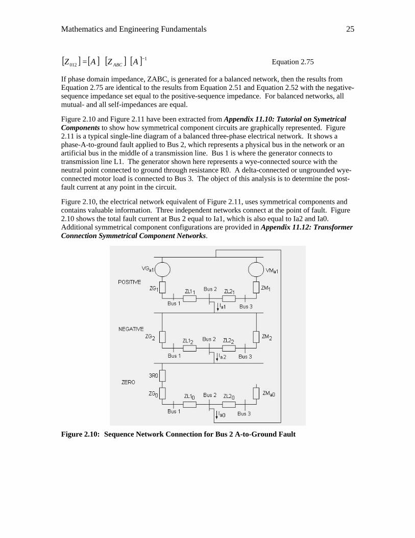
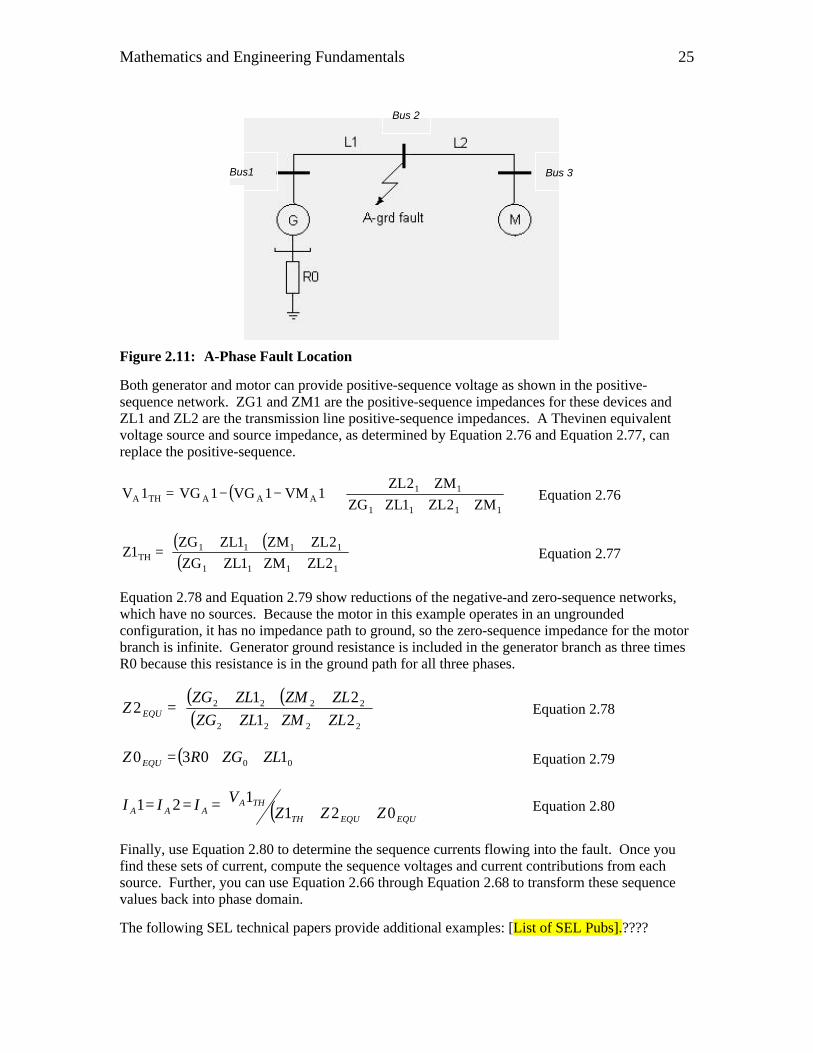
Figure 2.10 and Figure 2.11 have been extracted from Appendix 11.10: Tutorial on Symetrical Components to show how symmetrical component circuits are graphically represented. Figure 2.11 is a typical single-line diagram of a balanced three-phase electrical network. It shows a phase-A-to-ground fault applied to Bus 2, which represents a physical bus in the network or an artificial bus in the middle of a transmission line. Bus 1 is where the generator connects to transmission line L1. The generator shown here represents a wye-connected source with the neutral point connected to ground through resistance R0. A delta-connected or ungrounded wye-connected motor load is connected to Bus 3. The object of this analysis is to determine the post-fault current at any point in the circuit.
Figure 2.10, the electrical network equivalent of Figure 2.11, uses symmetrical components and contains valuable information. Three independent networks connect at the point of fault. Figure 2.10 shows the total fault current at Bus 2 equal to Ia1, which is also equal to Ia2 and Ia0. Additional symmetrical component configurations are provided in Appendix 11.12: Transformer Connection Symmetrical Component Networks.
Figure 2.10: Sequence Network Connection for Bus 2 A-to-Ground Fault
Mathematics and Engineering Fundamentals 25
Bus1
Bus 2
Bus 3
Figure 2.11: A-Phase Fault Location
Both generator and motor can provide positive-sequence voltage as shown in the positive-sequence network. ZG1 and ZM1 are the positive-sequence impedances for these devices and ZL1 and ZL2 are the transmission line positive-sequence impedances. A Thevinen equivalent voltage source and source impedance, as determined by Equation 2.76 and Equation 2.77, can replace the positive-sequence.
( )
+++
+⋅−−=
1111
11AAATHA ZM2ZL1ZLZG
ZM2ZL1VM1VG1VG1V Equation 2.76
( ) ( )( )
++++⋅+
=1111
1111TH 2ZLZM1ZLZG
2ZLZM1ZLZG1Z Equation 2.77
Equation 2.78 and Equation 2.79 show reductions of the negative-and zero-sequence networks, which have no sources. Because the motor in this example operates in an ungrounded configuration, it has no impedance path to ground, so the zero-sequence impedance for the motor branch is infinite. Generator ground resistance is included in the generator branch as three times R0 because this resistance is in the ground path for all three phases.
( ) ( )( )
++++⋅+
=2222
2222
21
212
ZLZMZLZG
ZLZMZLZGZ EQU Equation 2.78
( )00 1030 ZLZGRZ EQU ++= Equation 2.79
( )
++===EQUEQUTH
THAAAA ZZZ
VIII 021121 Equation 2.80
Finally, use Equation 2.80 to determine the sequence currents flowing into the fault. Once you find these sets of current, compute the sequence voltages and current contributions from each source. Further, you can use Equation 2.66 through Equation 2.68 to transform these sequence values back into phase domain.
The following SEL technical papers provide additional examples: [List of SEL Pubs].????

Mathematics and Engineering Fundamentals 25
Parks Equations
????
Faulted Systems—[Bosela Ch. 11, Pg. 371-404]????
The tools and approach for analyzing power systems depend on the purpose of the study and the state of the power system. Mathematical analyses of power systems have different perspectives depending on how rapidly the systems are expected to change. The three most common power system models in use today are steady-state, dynamic, and transient models.
Steady-State models
Steady-state solutions are appropriate for determining power transfer, nominal operating conditions, and initial and final conditions. The values for resistance, inductance, capacitance, and operating frequency that define the network do not change with time and the amplitude and phase of RMS voltages and currents are computed from complex impedances. Depending on the complexity of the network, complete the analysis using either hand calculations or computer-engineering programs to perform the phasor mathematics. Computer programs include spreadsheets, MathCAD, MATLAB, and power system analysis programs like Easy Flow.
Dynamic Models
Dynamic modeling assumes that the power system dynamics under consideration change at a rate significantly less than the power system frequency. Analyze these systems using Laplace transforms or differential equations. Like steady-state solutions, complex voltages, currents, and impedances make solutions independent of frequencies at and above the nominal power system frequency. Since the network changes with time, there are multiple solutions representing a series of steady-state conditions. MATLAB, MathCAD, and EMTP, addressed next, are suitable tools. Analog computer networks, called transient network analyzers, were once widely used, but have given way to computer-based solutions, which are both less expensive and more accurate.
Transient Models
Transient models result in time domain solutions. Voltages and currents produced by the mathematics are in effect samples of these signals. Networks are described using either discrete differential or difference equations that approximate linear differential equations to model inductors, capacitors, and electromechanical dynamics.
As with dynamic modeling, each new output is the result of solving the network equations of a system that is assumed to be momentarily in a steady-state condition. Each new solution becomes the initial condition for the next solution. The period representing the time between solutions limits the upper bounds of the frequency range included for a particular simulation. The same constraints that govern the validity of processes using digital filtering and sampled data systems, as discussed in paragraph 0, apply here.
When the program is first started, the initial conditions are computed using one of two methods. The first method is to generate a steady-state model as described in paragraph 0. Use Equation 2.9 to transfer the amplitude and phase results of this solution to the transient solution. This is not trivial because many of the difference equations need a history of many previous solutions to start off with a then correct next solution. With the advent of faster computers, this method has
Mathematics and Engineering Fundamentals 25
been replaced by simply letting the simulation start with zero initial conditions and running it long enough for initial transients to die out before initiating changes to the network.
Much research and engineering effort has been focused on improving computer transient simulations. Computer programs that are designed specifically to simulate transient responses for multiphase electrical networks are called Electromagnetic Transient Programs (EMTP). Some recent commercial products have developed real-time transient programs for testing instrumentation, monitoring, and control devices such as protective relays.
DIGITAL SYSTEMS
Digital systems include discrete signal theory and digital logic theory. Both use binary numbers to turn switches on and off. Computer control is often thought of in terms of Boolean operators such as AND, OR, and EXCLUSIVE OR. Computer control can also refer to algorithms that computers use to compute responses that, for relays, result in on-off controls as well as in reports that include numbers over a wide range of values. Discrete signal theory includes digital signal processing that uses computer algorithms to approximate analog filtering.
Signal Processing – Filtering Overview
Electromechanical relays are a type of analog filter. In the age of microprocessor-based relays, analog filters are still used for preprocessing, and in most cases, to mitigate high frequency noise caused by electrical transients, radio frequency interference (RFI), or electromagnetic interference (EMI). To understand this better, consider the following example. It is common practice to protect the CMOS ADC from overvoltage damage by connecting a surge protector from the input lead to chassis ground. Assume that a noise signal is coupled onto the circuit from an alien source and causes excessive voltage spikes. The transient-suppressing device clips (limits) the voltage magnitude and effectively protects the sensitive electronic circuits. However, clipping the signal magnitude corrupts the signal to be measured. Even if clipping does not actually alter the input signal, a new signal is now present. This new signal is the superposition sum of the original information signal and the noise.
For a filter to be effective, the noise must be in a different frequency band from that of the original signal in order to separate the good from the bad. If the noise is broadband, meaning that its energy is spread over a wide range of frequencies, filtering can help reduce the amount of corruption that the signal experiences. This is why most protective relays use analog filters.
Many microprocessor relays only respond to voltages and currents at 60 Hz. When the power system is in a state of change caused by normal switching operations or from faults, it generates other frequencies. The relay must first extract the 60 Hz information. The following brief example illustrates the need for filtering in relaying. Figure 2.12 shows a simple block diagram of the voltage and current analog input signal conditioning. The signal conversion provides scaling and possibly conversion to a voltage level appropriate for electronic devices.
SignalConversion
Low-passAnalogFilter
Sample &Band-pass
Filter
RMSConversion
MeasuredAnalogSignal
Magnitudeand Phase
Figure 2.12: Block Diagram of Relay Signal Conditioning and Conversion
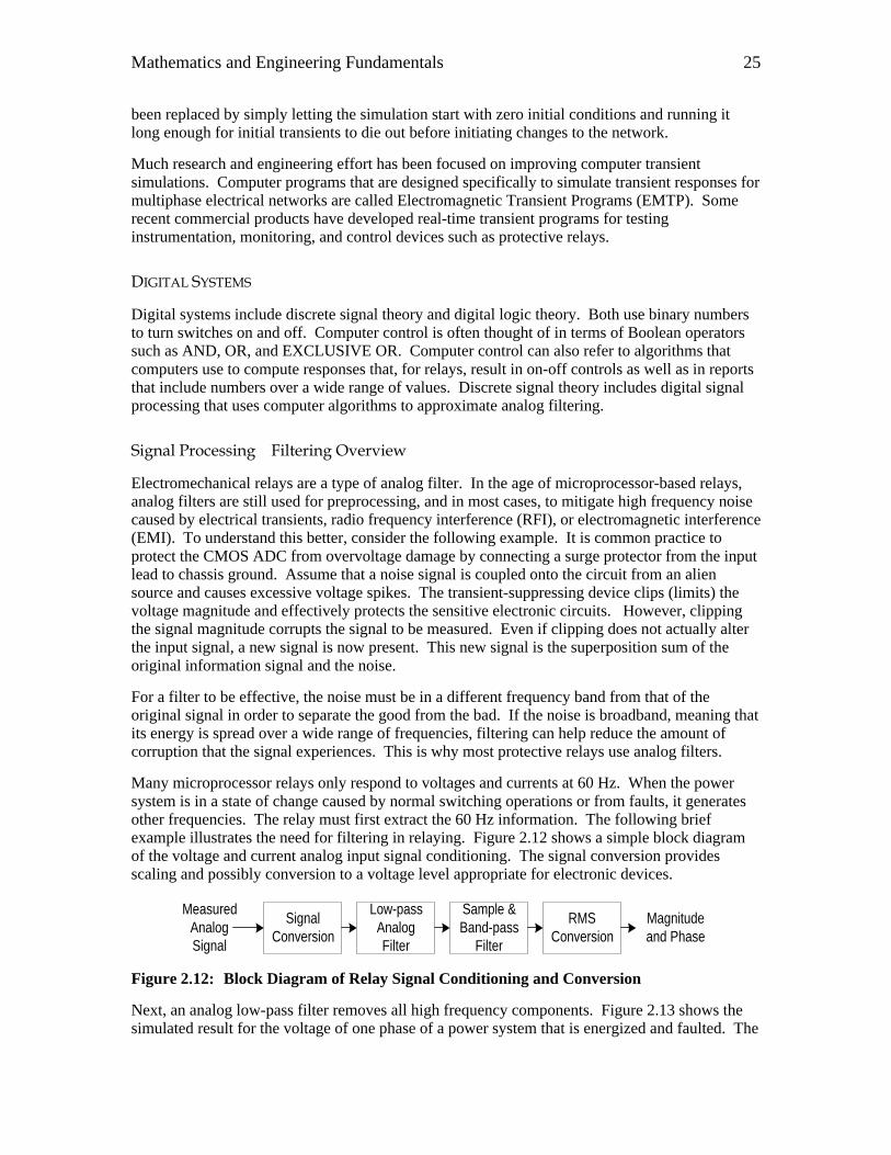
Next, an analog low-pass filter removes all high frequency components. Figure 2.13 shows the simulated result for the voltage of one phase of a power system that is energized and faulted. The
Mathematics and Engineering Fundamentals 25
analog filter removes some of the high frequency signals, but not all, depending on the filter design characteristics. For this example, the filter is second-order low-pass with a 3db cutoff set for 450 Hz. This plot also shows that there is a small but significant delay in the filtered signal. This delay shows up as phase shift for steady-state signals. Since all inputs pass through the same filter, the phase between signals remains constant. Keeping the cutoff frequency well above 60 Hz minimizes variations in delay caused by the component value deviations used to implement the analog low-pass filter.
Figure 2.13: Simulated Power System Transient
Mathematics and Engineering Fundamentals 25
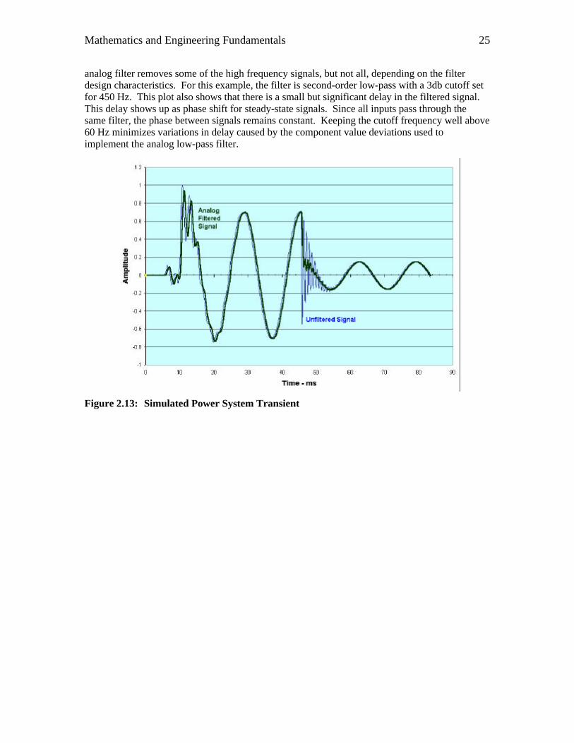
Figure 2.14: Frequency Spectrum of a Power System Transient Signal Before and After Analog Filtering
Figure 2.14 shows the frequency spectrum of the same two signals along with the analog filter response. The frequency response of the filtered signal is the simply the algebraic sum of the low-pass filter response and the input signal frequency spectrum at all corresponding frequencies. The low-pass filter characteristics have unity response until approximately 400 Hz and taper off to –3db at the 540 Hz cutoff frequency.
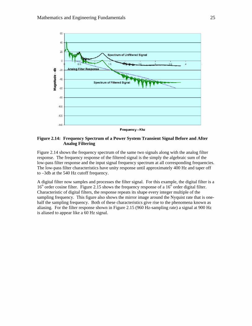
A digital filter now samples and processes the filter signal. For this example, the digital filter is a 16th order cosine filter. Figure 2.15 shows the frequency response of a 16th order digital filter. Characteristic of digital filters, the response repeats its shape every integer multiple of the sampling frequency. This figure also shows the mirror image around the Nyquist rate that is one-half the sampling frequency. Both of these characteristics give rise to the phenomena known as aliasing. For the filter response shown in Figure 2.15 (960 Hz-sampling rate) a signal at 900 Hz is aliased to appear like a 60 Hz signal.
Mathematics and Engineering Fundamentals 25
Figure 2.15: Frequency Response of a 16-Order Cosine Filter
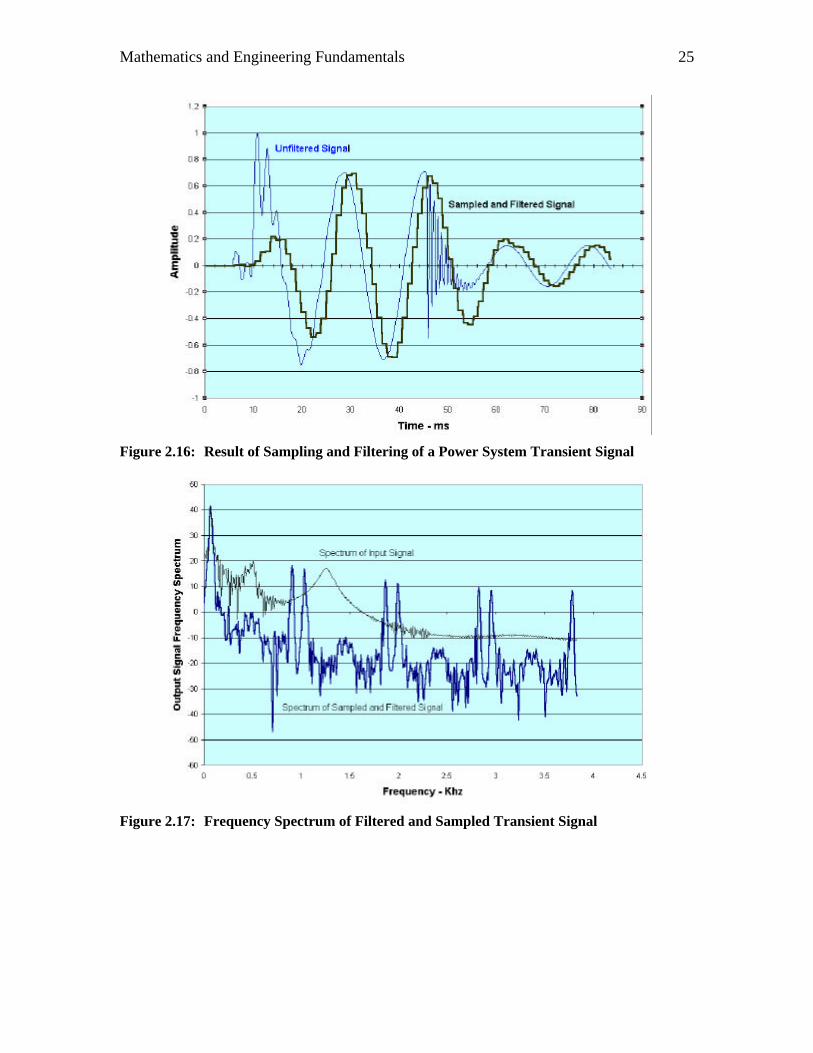
The output of this process shows the effects of sampling as well as of analog and digital filters. The delay resulting from the digital filter is more apparent in Figure 2.16. The processing delay is identical for all sampled inputs, resulting in no phase errors. However, the processing delay will also delay trip decisions made from processing this signal. This delay is a necessary overhead. The frequency spectrum of the sampled and filtered signal shown in Figure 2.17 reveals additional signal peaks that are not present in the original signal. This result of sampling produces the step changes in Figure 2.16.
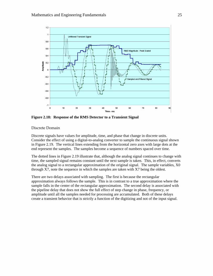
Figure 2.18 completes the process outlined in Figure 2.12. For convenience, the RMS magnitude is scaled for peak response by omitting the multiplication by √ ½ . Now that you have seen the application of filtering in relaying, the next few sections discuss the final issues of digital signal processing.
Mathematics and Engineering Fundamentals 25
Figure 2.16: Result of Sampling and Filtering of a Power System Transient Signal
Figure 2.17: Frequency Spectrum of Filtered and Sampled Transient Signal
Mathematics and Engineering Fundamentals 25
Figure 2.18: Response of the RMS Detector to a Transient Signal
Discrete Domain
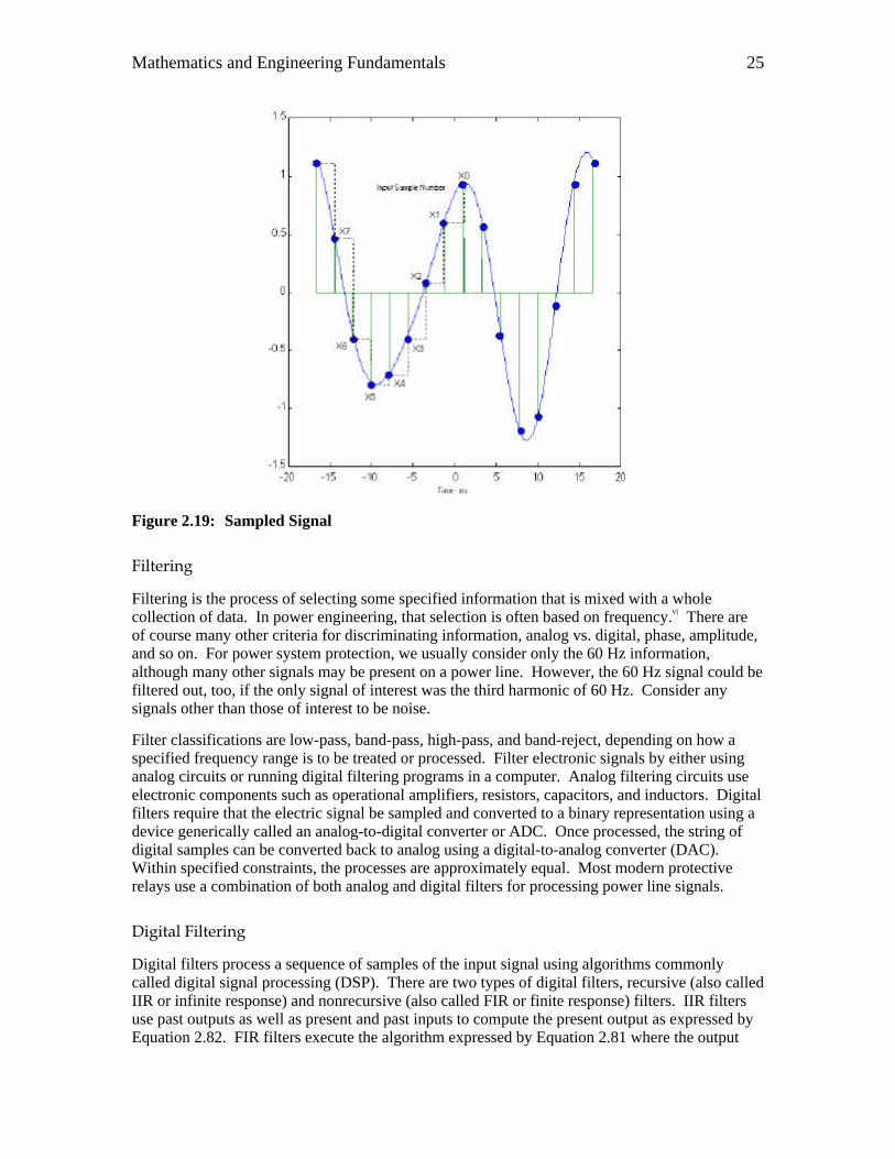
Discrete signals have values for amplitude, time, and phase that change in discrete units. Consider the effect of using a digital-to-analog converter to sample the continuous signal shown in Figure 2.19. The vertical lines extending from the horizontal zero axes with large dots at the end represent the samples. The samples become a sequence of numbers spaced over time.
The dotted lines in Figure 2.19 illustrate that, although the analog signal continues to change with time, the sampled signal remains constant until the next sample is taken. This, in effect, converts the analog signal to a rectangular approximation of the original signal. The sample variables, X0 through X7, note the sequence in which the samples are taken with X7 being the oldest.
There are two delays associated with sampling. The first is because the rectangular approximation always follows the sample. This is in contrast to a true approximation where the sample falls in the center of the rectangular approximation. The second delay is associated with the pipeline delay that does not show the full effect of step change in phase, frequency, or amplitude until all the samples needed for processing are accumulated. Both of these delays create a transient behavior that is strictly a function of the digitizing and not of the input signal.
Mathematics and Engineering Fundamentals 25
Figure 2.19: Sampled Signal
Filtering
Filtering is the process of selecting some specified information that is mixed with a whole collection of data. In power engineering, that selection is often based on frequency.vi There are of course many other criteria for discriminating information, analog vs. digital, phase, amplitude, and so on. For power system protection, we usually consider only the 60 Hz information, although many other signals may be present on a power line. However, the 60 Hz signal could be filtered out, too, if the only signal of interest was the third harmonic of 60 Hz. Consider any signals other than those of interest to be noise.
Filter classifications are low-pass, band-pass, high-pass, and band-reject, depending on how a specified frequency range is to be treated or processed. Filter electronic signals by either using analog circuits or running digital filtering programs in a computer. Analog filtering circuits use electronic components such as operational amplifiers, resistors, capacitors, and inductors. Digital filters require that the electric signal be sampled and converted to a binary representation using a device generically called an analog-to-digital converter or ADC. Once processed, the string of digital samples can be converted back to analog using a digital-to-analog converter (DAC). Within specified constraints, the processes are approximately equal. Most modern protective relays use a combination of both analog and digital filters for processing power line signals.
Digital Filtering
Digital filters process a sequence of samples of the input signal using algorithms commonly called digital signal processing (DSP). There are two types of digital filters, recursive (also called IIR or infinite response) and nonrecursive (also called FIR or finite response) filters. IIR filters use past outputs as well as present and past inputs to compute the present output as expressed by Equation 2.82. FIR filters execute the algorithm expressed by Equation 2.81 where the output
Mathematics and Engineering Fundamentals 25
from the filter, yk, is only dependent upon present and past input samples, xi. The process of determining the values of the coefficients that weight the inputs and outputs is beyond the scope of this treatment of digital filters, but is discussed in references. vii, viii
∑−
=
⋅=1
0
N
iiin bxy Equation 2.81
j
M
jjki
N
iin aybxy ⋅−⋅= ∑∑
−
=−
−
=
1
1)(
1
0
Equation 2.82
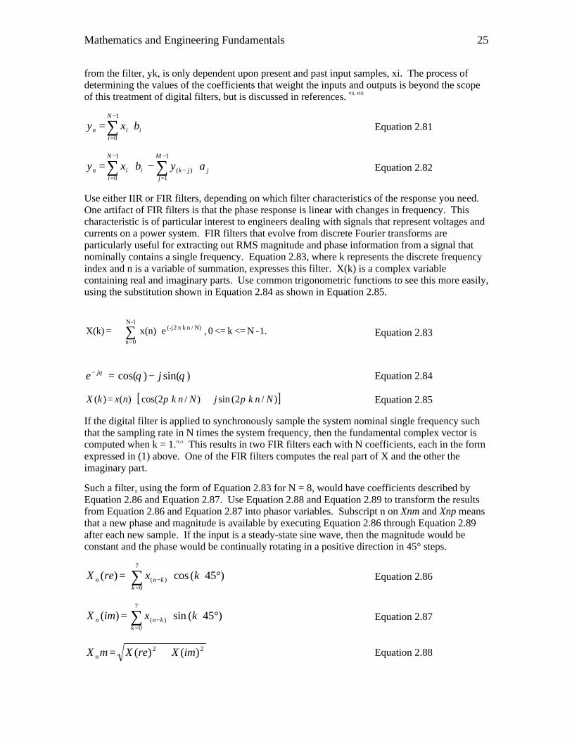
Use either IIR or FIR filters, depending on which filter characteristics of the response you need. One artifact of FIR filters is that the phase response is linear with changes in frequency. This characteristic is of particular interest to engineers dealing with signals that represent voltages and currents on a power system. FIR filters that evolve from discrete Fourier transforms are particularly useful for extracting out RMS magnitude and phase information from a signal that nominally contains a single frequency. Equation 2.83, where k represents the discrete frequency index and n is a variable of summation, expresses this filter. X(k) is a complex variable containing real and imaginary parts. Use common trigonometric functions to see this more easily, using the substitution shown in Equation 2.84 as shown in Equation 2.85.
1.-N k 0 , ex(n) X(k)
1-N
0n
N)/nk2(-j <=<== ∑=
π Equation 2.83
)sin()cos( θθθ je j −=− Equation 2.84
[ ])/2(sin)/2cos()()( NnkjNnknxkX ππ +⋅= Equation 2.85
If the digital filter is applied to synchronously sample the system nominal single frequency such that the sampling rate in N times the system frequency, then the fundamental complex vector is computed when k = 1.ix,x This results in two FIR filters each with N coefficients, each in the form expressed in (1) above. One of the FIR filters computes the real part of X and the other the imaginary part.
Such a filter, using the form of Equation 2.83 for N = 8, would have coefficients described by Equation 2.86 and Equation 2.87. Use Equation 2.88 and Equation 2.89 to transform the results from Equation 2.86 and Equation 2.87 into phasor variables. Subscript n on Xnm and Xnp means that a new phase and magnitude is available by executing Equation 2.86 through Equation 2.89 after each new sample. If the input is a steady-state sine wave, then the magnitude would be constant and the phase would be continually rotating in a positive direction in 45° steps.
∑=
− °⋅=7
0)( )45(cos)(
kknn kxreX Equation 2.86
∑=
− °⋅=7
0)( )45(sin)(
kknn kximX Equation 2.87
22 )()( imXreXmX n += Equation 2.88
Mathematics and Engineering Fundamentals 25
= )(
)(arctan reXimXpX
n
nn Equation 2.89
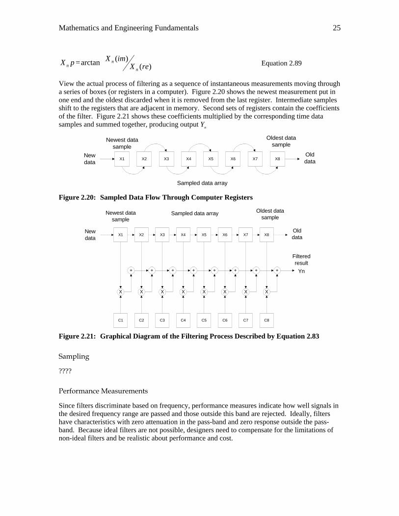
View the actual process of filtering as a sequence of instantaneous measurements moving through a series of boxes (or registers in a computer). Figure 2.20 shows the newest measurement put in one end and the oldest discarded when it is removed from the last register. Intermediate samples shift to the registers that are adjacent in memory. Second sets of registers contain the coefficients of the filter. Figure 2.21 shows these coefficients multiplied by the corresponding time data samples and summed together, producing output Yn
X1 X2 X3 X4 X5 X6 X7 X8
Sampled data array
Oldest datasample
Newest datasample
Newdata
Olddata
Figure 2.20: Sampled Data Flow Through Computer Registers
X1 X2 X3 X4 X5 X6 X7 X8
Sampled data array Oldest datasample
Newest datasample
Newdata
Olddata
C1 C2 C3 C4 C5 C6 C7 C8
+
X X X X X X X X
+ + + + + + + Yn
Filteredresult
Figure 2.21: Graphical Diagram of the Filtering Process Described by Equation 2.83
Sampling
????
Performance Measurements
Since filters discriminate based on frequency, performance measures indicate how well signals in the desired frequency range are passed and those outside this band are rejected. Ideally, filters have characteristics with zero attenuation in the pass-band and zero response outside the pass-band. Because ideal filters are not possible, designers need to compensate for the limitations of non-ideal filters and be realistic about performance and cost.
Mathematics and Engineering Fundamentals 25
Bandwidth
DFT filters have two more characteristics important to their applications to power system relaying: a response bandwidth and a transient response. The bandwidth of a filter is a two-edged sword. This filtering reduces the undesirable frequencies that can distort the phase and magnitude results. However, the ability to respond to a sudden change in amplitude is restricted even though the frequency of the signal remains unchanged.
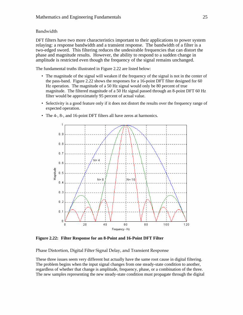
The fundamental truths illustrated in Figure 2.22 are listed below:
• The magnitude of the signal will weaken if the frequency of the signal is not in the center of the pass-band. Figure 2.22 shows the responses for a 16-point DFT filter designed for 60 Hz operation. The magnitude of a 50 Hz signal would only be 80 percent of true magnitude. The filtered magnitude of a 50 Hz signal passed through an 8-point DFT 60 Hz filter would be approximately 95 percent of actual value.
• Selectivity is a good feature only if it does not distort the results over the frequency range of expected operation.
• The 4-, 8-, and 16-point DFT filters all have zeros at harmonics.
Figure 2.22: Filter Response for an 8-Point and 16-Point DFT Filter
Phase Distortion, Digital Filter Signal Delay, and Transient Response
These three issues seem very different but actually have the same root cause in digital filtering. The problem begins when the input signal changes from one steady-state condition to another, regardless of whether that change is amplitude, frequency, phase, or a combination of the three. The new samples representing the new steady-state condition must propagate through the digital
Mathematics and Engineering Fundamentals 25
filters pipeline as illustrated in Figure 2.20 and Figure 2.21. Only after all input array values are replaced does the filter output accurately represent the response to the new steady-state condition.
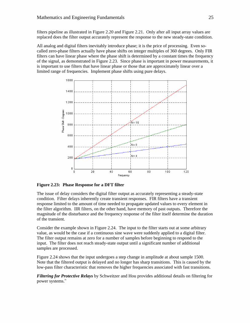
All analog and digital filters inevitably introduce phase; it is the price of processing. Even so-called zero-phase filters actually have phase shifts on integer multiples of 360 degrees. Only FIR filters can have linear phase where the phase shift is determined by a constant times the frequency of the signal, as demonstrated in Figure 2.23. Since phase is important in power measurements, it is important to use filters that have linear phase or those that are approximately linear over a limited range of frequencies. Implement phase shifts using pure delays.
Figure 2.23: Phase Response for a DFT filter
The issue of delay considers the digital filter output as accurately representing a steady-state condition. Filter delays inherently create transient responses. FIR filters have a transient response limited to the amount of time needed to propagate updated values to every element in the filter algorithm. IIR filters, on the other hand, have memory of past outputs. Therefore the magnitude of the disturbance and the frequency response of the filter itself determine the duration of the transient.
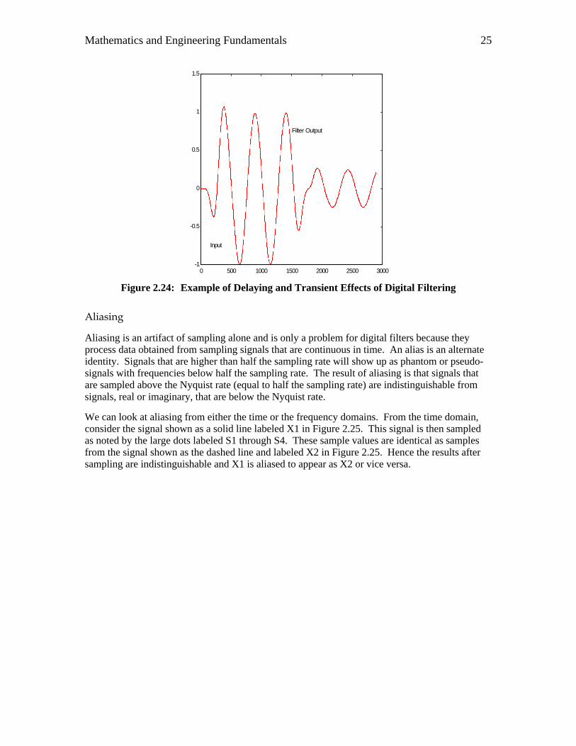
Consider the example shown in Figure 2.24. The input to the filter starts out at some arbitrary value, as would be the case if a continuous sine wave were suddenly applied to a digital filter. The filter output remains at zero for a number of samples before beginning to respond to the input. The filter does not reach steady-state output until a significant number of additional samples are processed.
Figure 2.24 shows that the input undergoes a step change in amplitude at about sample 1500. Note that the filtered output is delayed and no longer has sharp transitions. This is caused by the low-pass filter characteristic that removes the higher frequencies associated with fast transitions.
Filtering for Protective Relays by Schweitzer and Hou provides additional details on filtering for power systems.ix
Mathematics and Engineering Fundamentals 25
0 500 1000 1500 2000 2500 3000-1
-0.5
0
0.5
1
1.5
Input
Filter Output
Figure 2.24: Example of Delaying and Transient Effects of Digital Filtering
Aliasing
Aliasing is an artifact of sampling alone and is only a problem for digital filters because they process data obtained from sampling signals that are continuous in time. An alias is an alternate identity. Signals that are higher than half the sampling rate will show up as phantom or pseudo-signals with frequencies below half the sampling rate. The result of aliasing is that signals that are sampled above the Nyquist rate (equal to half the sampling rate) are indistinguishable from signals, real or imaginary, that are below the Nyquist rate.
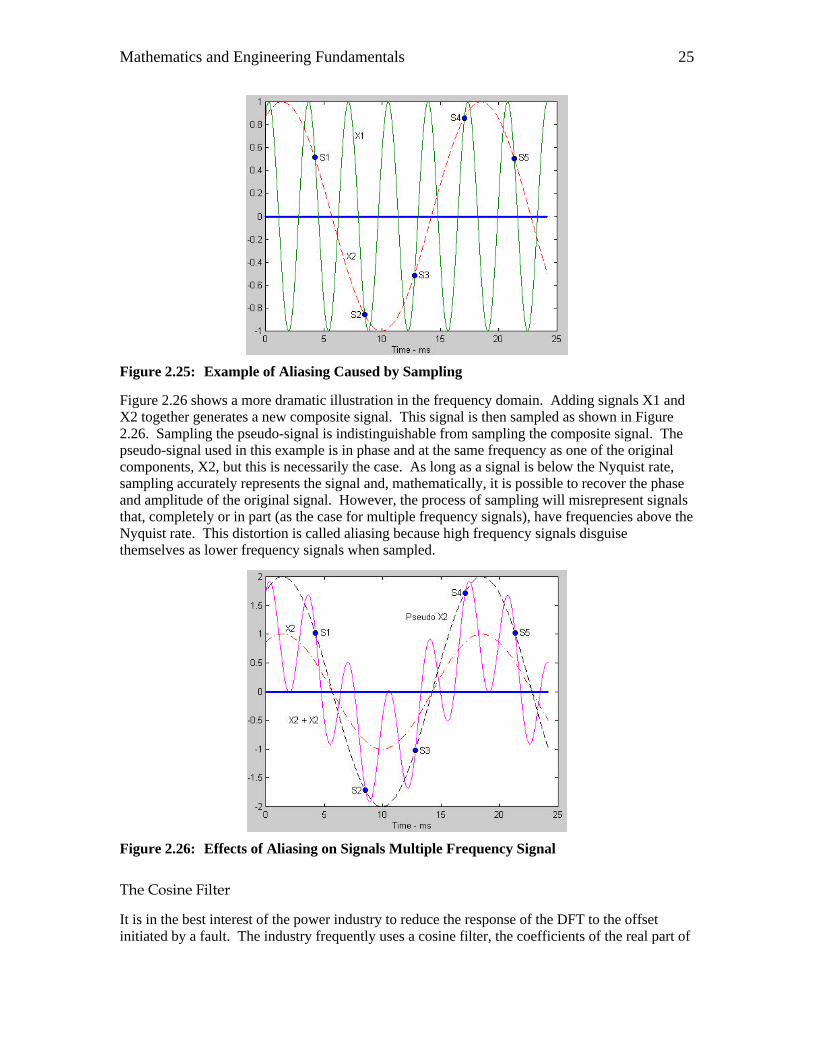
We can look at aliasing from either the time or the frequency domains. From the time domain, consider the signal shown as a solid line labeled X1 in Figure 2.25. This signal is then sampled as noted by the large dots labeled S1 through S4. These sample values are identical as samples from the signal shown as the dashed line and labeled X2 in Figure 2.25. Hence the results after sampling are indistinguishable and X1 is aliased to appear as X2 or vice versa.
Mathematics and Engineering Fundamentals 25
Figure 2.25: Example of Aliasing Caused by Sampling
Figure 2.26 shows a more dramatic illustration in the frequency domain. Adding signals X1 and X2 together generates a new composite signal. This signal is then sampled as shown in Figure 2.26. Sampling the pseudo-signal is indistinguishable from sampling the composite signal. The pseudo-signal used in this example is in phase and at the same frequency as one of the original components, X2, but this is necessarily the case. As long as a signal is below the Nyquist rate, sampling accurately represents the signal and, mathematically, it is possible to recover the phase and amplitude of the original signal. However, the process of sampling will misrepresent signals that, completely or in part (as the case for multiple frequency signals), have frequencies above the Nyquist rate. This distortion is called aliasing because high frequency signals disguise themselves as lower frequency signals when sampled.
Figure 2.26: Effects of Aliasing on Signals Multiple Frequency Signal
The Cosine Filter
It is in the best interest of the power industry to reduce the response of the DFT to the offset initiated by a fault. The industry frequently uses a cosine filter, the coefficients of the real part of
Mathematics and Engineering Fundamentals 25
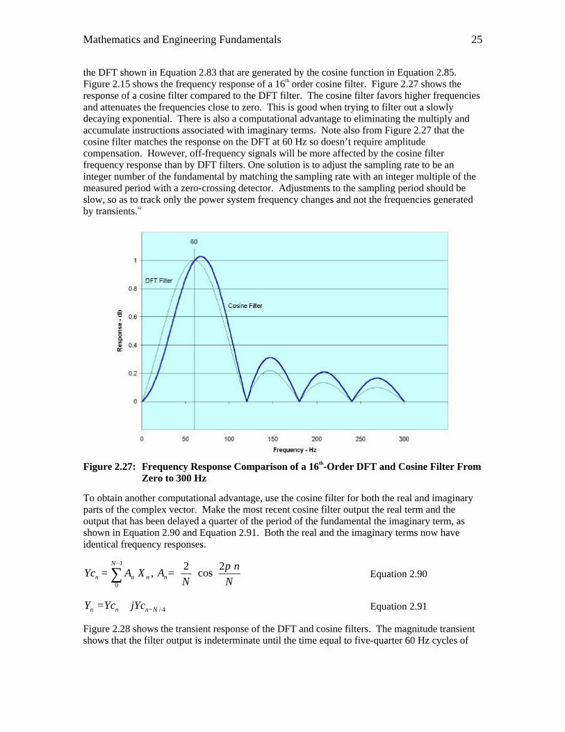
the DFT shown in Equation 2.83 that are generated by the cosine function in Equation 2.85. Figure 2.15 shows the frequency response of a 16th order cosine filter. Figure 2.27 shows the response of a cosine filter compared to the DFT filter. The cosine filter favors higher frequencies and attenuates the frequencies close to zero. This is good when trying to filter out a slowly decaying exponential. There is also a computational advantage to eliminating the multiply and accumulate instructions associated with imaginary terms. Note also from Figure 2.27 that the cosine filter matches the response on the DFT at 60 Hz so doesn’t require amplitude compensation. However, off-frequency signals will be more affected by the cosine filter frequency response than by DFT filters. One solution is to adjust the sampling rate to be an integer number of the fundamental by matching the sampling rate with an integer multiple of the measured period with a zero-crossing detector. Adjustments to the sampling period should be slow, so as to track only the power system frequency changes and not the frequencies generated by transients.xi
Figure 2.27: Frequency Response Comparison of a 16th-Order DFT and Cosine Filter From Zero to 300 Hz
To obtain another computational advantage, use the cosine filter for both the real and imaginary parts of the complex vector. Make the most recent cosine filter output the real term and the output that has been delayed a quarter of the period of the fundamental the imaginary term, as shown in Equation 2.90 and Equation 2.91. Both the real and the imaginary terms now have identical frequency responses.
== ∑
−
N
n
NAXAYc n
N
nnn
π2cos
2,
1
0
Equation 2.90
4/Nnnn jYcYcY −+= Equation 2.91
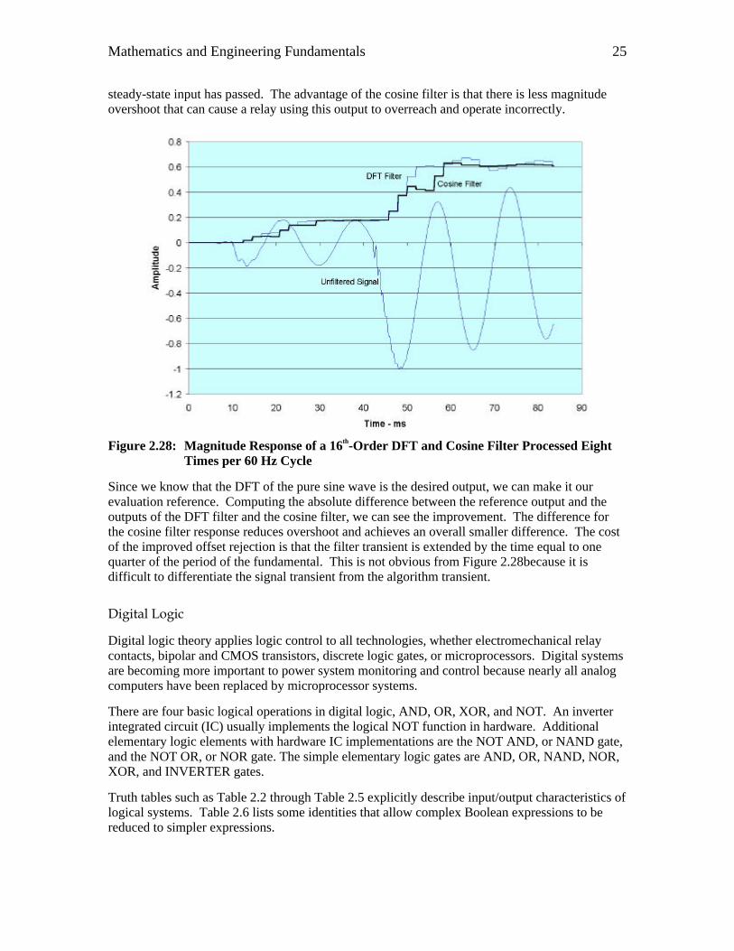
Figure 2.28 shows the transient response of the DFT and cosine filters. The magnitude transient shows that the filter output is indeterminate until the time equal to five-quarter 60 Hz cycles of
Mathematics and Engineering Fundamentals 25
steady-state input has passed. The advantage of the cosine filter is that there is less magnitude overshoot that can cause a relay using this output to overreach and operate incorrectly.
Figure 2.28: Magnitude Response of a 16th-Order DFT and Cosine Filter Processed Eight Times per 60 Hz Cycle
Since we know that the DFT of the pure sine wave is the desired output, we can make it our evaluation reference. Computing the absolute difference between the reference output and the outputs of the DFT filter and the cosine filter, we can see the improvement. The difference for the cosine filter response reduces overshoot and achieves an overall smaller difference. The cost of the improved offset rejection is that the filter transient is extended by the time equal to one quarter of the period of the fundamental. This is not obvious from Figure 2.28because it is difficult to differentiate the signal transient from the algorithm transient.
Digital Logic
Digital logic theory applies logic control to all technologies, whether electromechanical relay contacts, bipolar and CMOS transistors, discrete logic gates, or microprocessors. Digital systems are becoming more important to power system monitoring and control because nearly all analog computers have been replaced by microprocessor systems.
There are four basic logical operations in digital logic, AND, OR, XOR, and NOT. An inverter integrated circuit (IC) usually implements the logical NOT function in hardware. Additional elementary logic elements with hardware IC implementations are the NOT AND, or NAND gate, and the NOT OR, or NOR gate. The simple elementary logic gates are AND, OR, NAND, NOR, XOR, and INVERTER gates.
Truth tables such as Table 2.2 through Table 2.5 explicitly describe input/output characteristics of logical systems. Table 2.6 lists some identities that allow complex Boolean expressions to be reduced to simpler expressions.
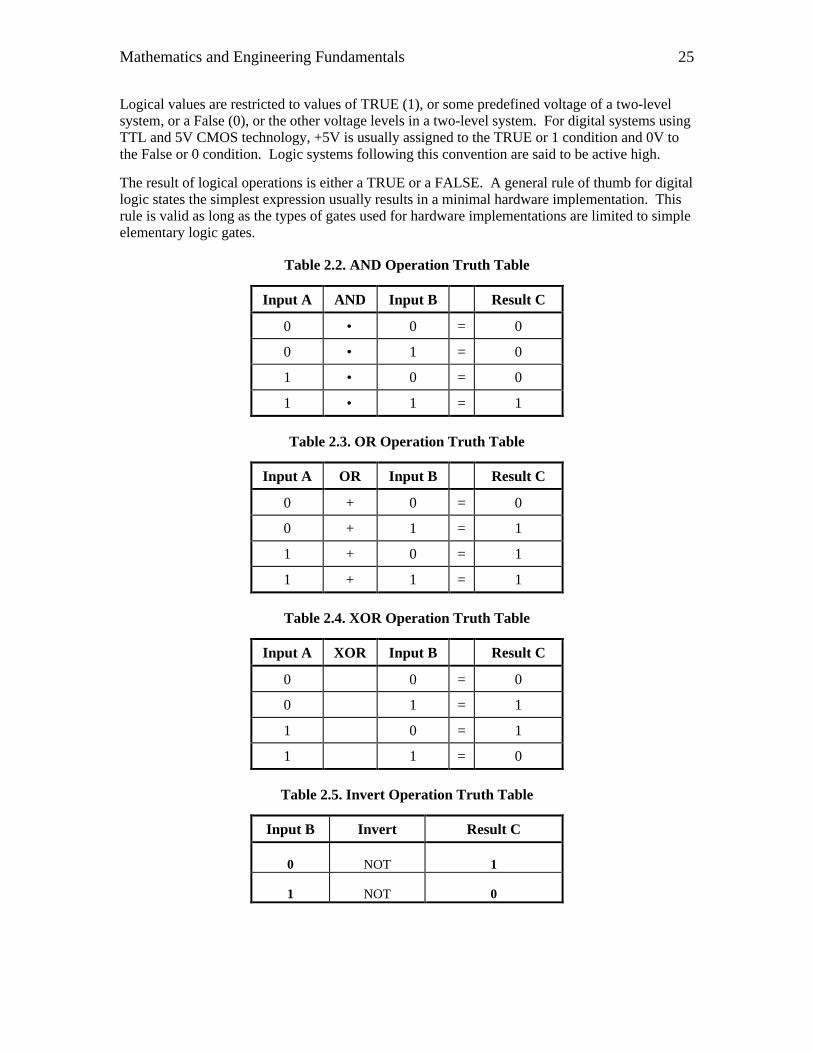
Mathematics and Engineering Fundamentals 25
Logical values are restricted to values of TRUE (1), or some predefined voltage of a two-level system, or a False (0), or the other voltage levels in a two-level system. For digital systems using TTL and 5V CMOS technology, +5V is usually assigned to the TRUE or 1 condition and 0V to the False or 0 condition. Logic systems following this convention are said to be active high.
The result of logical operations is either a TRUE or a FALSE. A general rule of thumb for digital logic states the simplest expression usually results in a minimal hardware implementation. This rule is valid as long as the types of gates used for hardware implementations are limited to simple elementary logic gates.
Table 2.2. AND Operation Truth Table
Input A AND Input B Result C
0 • 0 = 0
0 • 1 = 0
1 • 0 = 0
1 • 1 = 1
Table 2.3. OR Operation Truth Table
Input A OR Input B Result C
0 + 0 = 0
0 + 1 = 1
1 + 0 = 1
1 + 1 = 1
Table 2.4. XOR Operation Truth Table
Input A XOR Input B Result C
0 ⊕ 0 = 0
0 ⊕ 1 = 1
1 ⊕ 0 = 1
1 ⊕ 1 = 0
Table 2.5. Invert Operation Truth Table
Input B Invert Result C
0 NOT 1
1 NOT 0
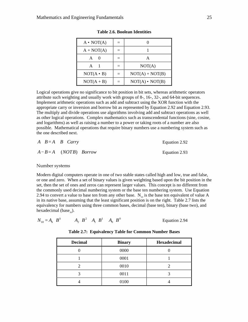
Mathematics and Engineering Fundamentals 25
Table 2.6. Boolean Identities
A • NOT(A) = 0
A + NOT(A) = 1
A ⊕ 0 = A
A ⊕ 1 = NOT(A)
NOT(A • B) = NOT(A) + NOT(B)
NOT(A + B) = NOT(A) • NOT(B)
Logical operations give no significance to bit position in bit sets, whereas arithmetic operators attribute such weighting and usually work with groups of 8-, 16-, 32-, and 64-bit sequences. Implement arithmetic operations such as add and subtract using the XOR function with the appropriate carry or inversion and borrow bit as represented by Equation 2.92 and Equation 2.93. The multiply and divide operations use algorithms involving add and subtract operations as well as other logical operations. Complex mathematics such as transcendental functions (sine, cosine, and logarithms) as well as raising a number to a power or taking roots of a number are also possible. Mathematical operations that require binary numbers use a numbering system such as the one described next.
CarryBABA +⊕=+ Equation 2.92
BorrowBNOTABA +⊕=− )( Equation 2.93
Number systems
Modern digital computers operate in one of two stable states called high and low, true and false, or one and zero. When a set of binary values is given weighting based upon the bit position in the set, then the set of ones and zeros can represent larger values. This concept is no different from the commonly used decimal numbering system or the base ten numbering system. Use Equation 2.94 to convert a value to base ten from any other base. N10 is the base ten equivalent of value A in its native base, assuming that the least significant position is on the right. Table 2.7 lists the equivalency for numbers using three common bases, decimal (base ten), binary (base two), and hexadecimal (base16).
00
11
2210 BABABABAN k
k ⋅+⋅+⋅+⋅⋅⋅+⋅= Equation 2.94
Table 2.7: Equivalency Table for Common Number Bases
Decimal Binary Hexadecimal
0 0000 0
1 0001 1
2 0010 2
3 0011 3
4 0100 4
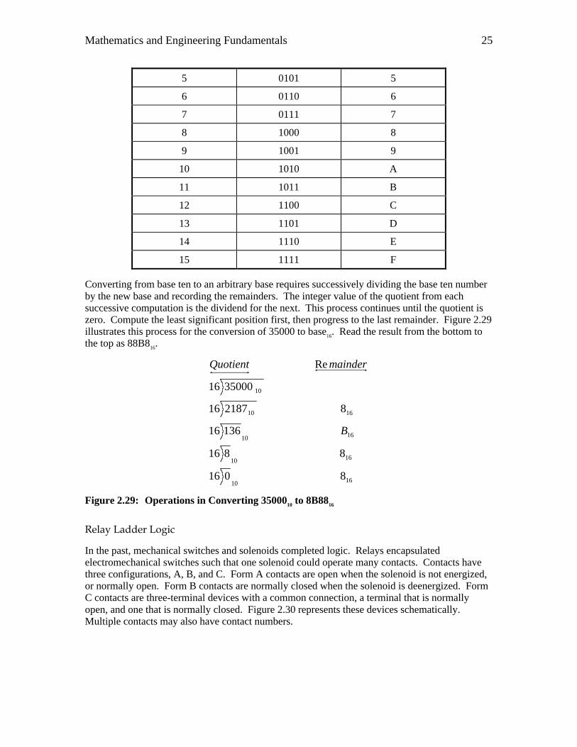
Mathematics and Engineering Fundamentals 25
5 0101 5
6 0110 6
7 0111 7
8 1000 8
9 1001 9
10 1010 A
11 1011 B
12 1100 C
13 1101 D
14 1110 E
15 1111 F
Converting from base ten to an arbitrary base requires successively dividing the base ten number by the new base and recording the remainders. The integer value of the quotient from each successive computation is the dividend for the next. This process continues until the quotient is zero. Compute the least significant position first, then progress to the last remainder. Figure 2.29 illustrates this process for the conversion of 35000 to base16. Read the result from the bottom to the top as 88B816.
1610
1610
1610
1610
10
8016
8816
13616
8218716
3500016
Re
B
mainderQuotient
Figure 2.29: Operations in Converting 3500010 to 8B8816
Relay Ladder Logic
In the past, mechanical switches and solenoids completed logic. Relays encapsulated electromechanical switches such that one solenoid could operate many contacts. Contacts have three configurations, A, B, and C. Form A contacts are open when the solenoid is not energized, or normally open. Form B contacts are normally closed when the solenoid is deenergized. Form C contacts are three-terminal devices with a common connection, a terminal that is normally open, and one that is normally closed. Figure 2.30 represents these devices schematically. Multiple contacts may also have contact numbers.
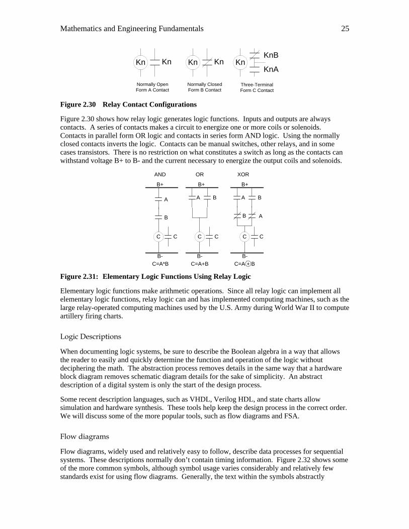
Mathematics and Engineering Fundamentals 25
Kn KnKnKn
Normally OpenForm A Contact
Normally ClosedForm B Contact
Three-TerminalForm C Contact
KnKnB
KnA
Figure 2.30 Relay Contact Configurations
Figure 2.30 shows how relay logic generates logic functions. Inputs and outputs are always contacts. A series of contacts makes a circuit to energize one or more coils or solenoids. Contacts in parallel form OR logic and contacts in series form AND logic. Using the normally closed contacts inverts the logic. Contacts can be manual switches, other relays, and in some cases transistors. There is no restriction on what constitutes a switch as long as the contacts can withstand voltage B+ to B- and the current necessary to energize the output coils and solenoids.
C
A
B
C C
A B
C C
A B
C
B A
B+
B- B- B-
B+ B+
AND OR XOR
C=A*B C=A+B C=A + B
Figure 2.31: Elementary Logic Functions Using Relay Logic
Elementary logic functions make arithmetic operations. Since all relay logic can implement all elementary logic functions, relay logic can and has implemented computing machines, such as the large relay-operated computing machines used by the U.S. Army during World War II to compute artillery firing charts.
Logic Descriptions
When documenting logic systems, be sure to describe the Boolean algebra in a way that allows the reader to easily and quickly determine the function and operation of the logic without deciphering the math. The abstraction process removes details in the same way that a hardware block diagram removes schematic diagram details for the sake of simplicity. An abstract description of a digital system is only the start of the design process.
Some recent description languages, such as VHDL, Verilog HDL, and state charts allow simulation and hardware synthesis. These tools help keep the design process in the correct order. We will discuss some of the more popular tools, such as flow diagrams and FSA.
Flow diagrams
Flow diagrams, widely used and relatively easy to follow, describe data processes for sequential systems. These descriptions normally don’t contain timing information. Figure 2.32 shows some of the more common symbols, although symbol usage varies considerably and relatively few standards exist for using flow diagrams. Generally, the text within the symbols abstractly
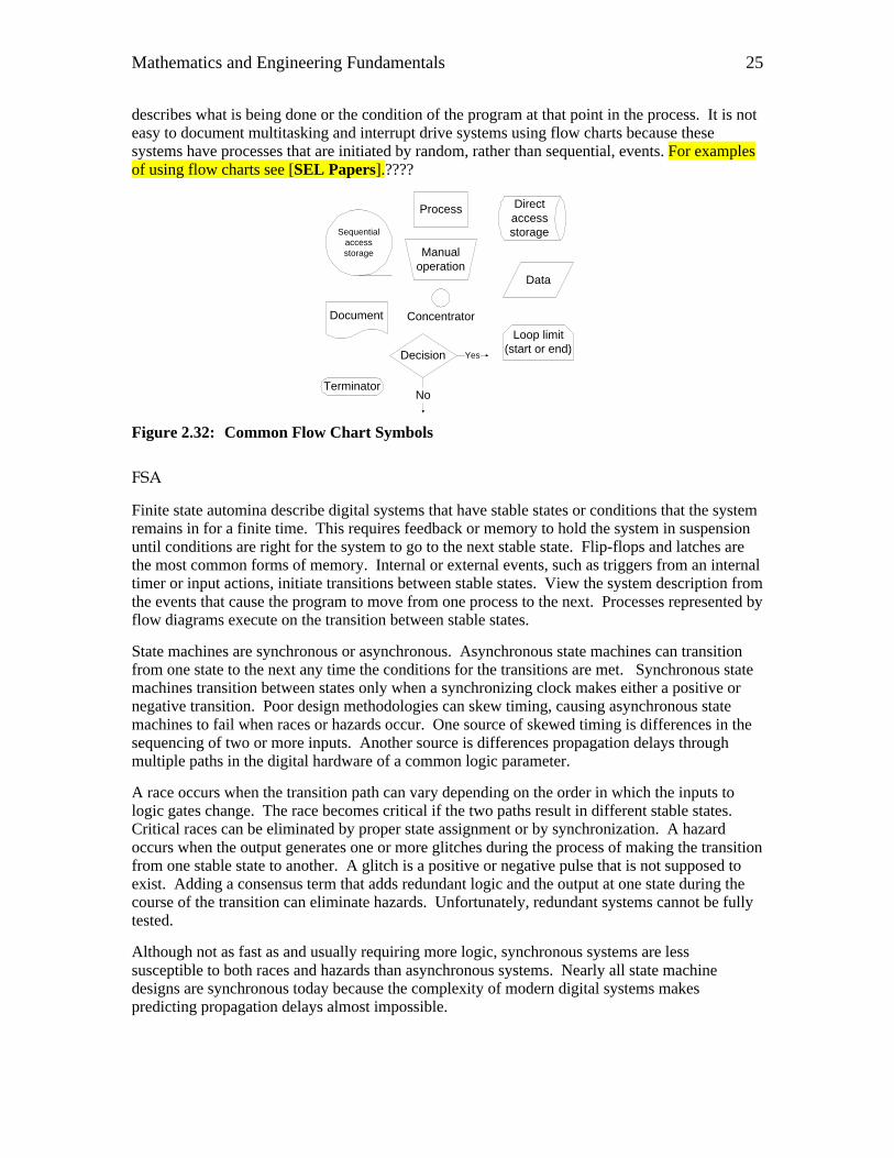
Mathematics and Engineering Fundamentals 25
describes what is being done or the condition of the program at that point in the process. It is not easy to document multitasking and interrupt drive systems using flow charts because these systems have processes that are initiated by random, rather than sequential, events. For examples of using flow charts see [SEL Papers].????
Process
Data
Decision
Document
Sequentialaccessstorage
Directaccessstorage
Terminator
Loop limit(start or end)
Manualoperation
Concentrator
No
Yes
Figure 2.32: Common Flow Chart Symbols
FSA
Finite state automina describe digital systems that have stable states or conditions that the system remains in for a finite time. This requires feedback or memory to hold the system in suspension until conditions are right for the system to go to the next stable state. Flip-flops and latches are the most common forms of memory. Internal or external events, such as triggers from an internal timer or input actions, initiate transitions between stable states. View the system description from the events that cause the program to move from one process to the next. Processes represented by flow diagrams execute on the transition between stable states.
State machines are synchronous or asynchronous. Asynchronous state machines can transition from one state to the next any time the conditions for the transitions are met. Synchronous state machines transition between states only when a synchronizing clock makes either a positive or negative transition. Poor design methodologies can skew timing, causing asynchronous state machines to fail when races or hazards occur. One source of skewed timing is differences in the sequencing of two or more inputs. Another source is differences propagation delays through multiple paths in the digital hardware of a common logic parameter.
A race occurs when the transition path can vary depending on the order in which the inputs to logic gates change. The race becomes critical if the two paths result in different stable states. Critical races can be eliminated by proper state assignment or by synchronization. A hazard occurs when the output generates one or more glitches during the process of making the transition from one stable state to another. A glitch is a positive or negative pulse that is not supposed to exist. Adding a consensus term that adds redundant logic and the output at one state during the course of the transition can eliminate hazards. Unfortunately, redundant systems cannot be fully tested.
Although not as fast as and usually requiring more logic, synchronous systems are less susceptible to both races and hazards than asynchronous systems. Nearly all state machine designs are synchronous today because the complexity of modern digital systems makes predicting propagation delays almost impossible.
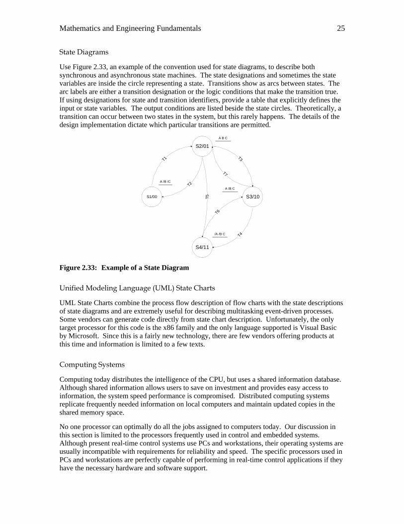
Mathematics and Engineering Fundamentals 25
State Diagrams
Use Figure 2.33, an example of the convention used for state diagrams, to describe both synchronous and asynchronous state machines. The state designations and sometimes the state variables are inside the circle representing a state. Transitions show as arcs between states. The arc labels are either a transition designation or the logic conditions that make the transition true. If using designations for state and transition identifiers, provide a table that explicitly defines the input or state variables. The output conditions are listed beside the state circles. Theoretically, a transition can occur between two states in the system, but this rarely happens. The details of the design implementation dictate which particular transitions are permitted.
S1/00
S2/01
S3/10
S4/11
T1 T3
T4
T2
T5
T6
/A /B C
A /B /C
A /B C
A B C
T7
Figure 2.33: Example of a State Diagram
Unified Modeling Language (UML) State Charts
UML State Charts combine the process flow description of flow charts with the state descriptions of state diagrams and are extremely useful for describing multitasking event-driven processes. Some vendors can generate code directly from state chart description. Unfortunately, the only target processor for this code is the x86 family and the only language supported is Visual Basic by Microsoft. Since this is a fairly new technology, there are few vendors offering products at this time and information is limited to a few texts.
Computing Systems
Computing today distributes the intelligence of the CPU, but uses a shared information database. Although shared information allows users to save on investment and provides easy access to information, the system speed performance is compromised. Distributed computing systems replicate frequently needed information on local computers and maintain updated copies in the shared memory space.
No one processor can optimally do all the jobs assigned to computers today. Our discussion in this section is limited to the processors frequently used in control and embedded systems. Although present real-time control systems use PCs and workstations, their operating systems are usually incompatible with requirements for reliability and speed. The specific processors used in PCs and workstations are perfectly capable of performing in real-time control applications if they have the necessary hardware and software support.

Mathematics and Engineering Fundamentals 25
Processor classifications fall along different lines. Processors use either the von Neumann architecture (shared with code and data bus) or Harvard architecture (separate code and data bus). Harvard architecture computers are generally faster and have larger memory capability; they are also more complex and have difficulty operating on nonvolatile data stored in the code memory space. Such differences are largely transparent to the programmer.
For convenience, we will maintain three further computer classifications: complex instruction set computers (CISC), reduced instruction set computers (RISC), and digital signal processors (DSP). Pentium processors are CISC and have instructions that require varying numbers of bytes. Some instructions involve compound operations such as the integer multiply, divide, and decrement-and-branch-if-zero instructions. It is difficult to learn the assembler language for such processors because of the quantity and complexity of the commands. Fortunately, high-level language programming insulates developers from most of these issues.
RISC processors use a minimal number of primitive instructions that execute one instruction per word. In this context, the word is a native width for code that is fetched using a single fetch operation. RISC processors are pipelined so that the processor can be simultaneously fetching and executing. There is still debate about whether CISC or RISC computers are faster and require less memory to complete tasks. The answer usually depends on the benchmark being used for the comparison.
DSP processors are really a subclass of RISC processors with additional computing hardware that makes them particularly efficient for executing multiply and accumulate (MAC) instructions. Digital filtering algorithms use these instructions repeatedly, as discussed in paragraph 0. In addition to the conventional ALU contained in all computers, DSP processors also have a hardware multiplier and hardware adder that can operate in parallel with each other as well as with the ALU. A single word, usually 16 bits in width or greater, contains instructions, which are also divided into control fields that determine the operation for the ALU, multiplier, and adder.
Microprocessors and Microcontrollers
The usual consensus about the difference between microprocessors and microcontrollers is that microcontrollers are designed with a high degree of I/O capability and microprocessors are designed to handle large amounts of data efficiently. The two designs have more common characteristics than differences, but Table 2.8 lists some of these distinctions.
Table 2.8: Comparison of Microprocessors and Microcontrollers
Microprocessors Microcontrollers
Code Memory Large Small
Data Memory Large Small
Direct I/O pins Few Many
Autonomous operation No – needs O.S. Yes – O.S. built in
Number of Interrupt sources Few Many
Special functions Few Many
Cost High Low

Mathematics and Engineering Fundamentals 25
Refer to How Microprocessor Relays Respond to Harmonics, Saturation, and Other Wave Distortions by Stanley E. Zocholl and Gabriel Benmouyal for additional information.
Memory
Digital computer systems require both code memory and data memory. Code memory contains the instructions that the processor executes. For a given application, this memory should not change. Some programmers develop computers that produce self-generated or self-modified code. Avoid this practice, except for rare instances, because such code is not testable. The memory for storing code and constant data must be nonvolatile so that when the power is deenergized and reenergized, this memory is not destroyed. Masked ROM, OTP ROM, UV-EPROM, EE-EPROM, FLASH memory, and battery backed-up static RAM are common technologies for nonvolatile memory embedded systems. Larger computer-based systems may use a combination of these, as well as a mass-memory media such as floppy disk, hard disk, and CD ROM.
The computer must be able to modify memory for storing variable data, usually by static or dynamic RAM technologies. Computers that need to retain data after the system is deenergized may use nonvolatile memory that is easily modifiable such as battery backed-up static RAM, EEPROM, Flash memory or disk. Although the latter three options are less expensive, they also have limited lifetime write cycles and are considerably slower.
The amount of memory in a particular memory device is classified either by a single value representing the total number of memory bits or a two-dimensional array of the number of data bits wide by the number of address bytes deep. Dynamic memory in PCs is typically nine bits wide, having eight data bits and a one parity bit for error detection. In general, however, semiconductor memory is packaged as either eight or 16 bits wide. Disk memory is single-bit wide on the storage media but may be repackaged to a width suitable for the processor by a disk controller.
Equation 2.95 shows the depth of a memory device computed by the number of address lines.
linesaddressofNumberDepth 2= Equation 2.95
Input and Output
All microprocessors and many microcontrollers support access to external ROM and RAM memory devices. Access macro logic integrated circuits such as serial communications drivers (UARTS), interrupt controllers, analog-to-digital converters (ADC), and digital-to-analog converters (DAC) using memory address space and mapped-memory I/O.
Processors use three types of control lines or pins to access memory, both code and data, and mapped memory I/O; address lines, data lines, and control or hand-shaking lines. Use address and data lines for I/O devices in the same way as memory, discussed above. Data lines are bi-directional and are commonly shared with all devices that interface to the processor through the memory expansion lines.
Address decoding gives the processor a means to distinguish the access to one device from all the others connected to the external memory bus. Some processors have a set of chip-select control outputs while others rely on external ICs using combinational logic to decode specific address ranges and to generate the appropriate chip-select signals. Multiple address lines on an I/O device give the processor access to control, status, and data registers internal to the particular I/O

Mathematics and Engineering Fundamentals 25
device. For example, ICs that perform timekeeping functions typically have a register for the year, month, day, hour, minute, second, and tenth of a second. Other registers set up the timekeeping format. Since these timekeeping ICs have battery backup, there are often additional registers for applications requiring a small amount of nonvolatile memory. Such devices have five or more address lines to provide access to all the various internal registers.
Control lines, in addition to selecting the particular device to be accessed, also direct the flow of information on the data line either to or from the external I/O or memory device. Some processors share the address and data lines using time division multiplexing. The processor supplies a control line to signal when the shared address and data bus contain address information and when it is being used for data. Some ICs decode this signal directly, while others require external decoding and latching of address information.
Interrupts are special I/O control lines that require the processor to be managed by the user-developed code. These are hardware-generated program subroutine call instructions to a predetermined address. Mask bits that enable and disable their operation manage the interrupts. Catastrophic operations such as power failure require that some interrupts remain impervious to this disabling. These non-maskable interrupts are extremely useful for allowing a processor system to fail in a safe and predictable way.
Special Functions for Microcontrollers
Computers need special purpose semiconductor devices to expand processor I/O capability and functionality. These include analog input, pulse width modulation (PWM) for analog output, event timers, synchronous and asynchronous serial communications, and multiple access serial networks. Individual ICs, commonly used for microprocessors, can also provide the functions and services provided by these devices.
Microcontrollers frequently include the special hardware on the same silicon wafer as the processor. Since the intended use for the microcontroller is in systems that require a minimum of support hardware, integrating the special purpose hardware with the processor eliminates external addressing and improves the access speed.
Gate Arrays
Gate arrays are semiconductor devices containing hundreds of thousands of logic gates and flip-flops that are massively interconnected in a two-dimensional array. End users or customer-developers can use inexpensive devices to program field programmable gate arrays (FPGA). Programming these devices consists of retaining or eliminating interconnections between gates and flip-flops that subsequently generate the desired logic functions. System designers frequently use Gate arrays (extremely fast Boolean processors) to off-load computing requirements in a hardware-software co-design because either the processor is too slow or the demands would consume too much processor time. Gate array designs are quickly replacing designs using discrete logic circuits such as the 7400 series TTL and CMOS logic.
i Theodore Bosela, Introduction to Power System Technology, 1997, ISBN 0-13-186537-4, Prentice-Hall, Upper Saddle River, NJ.
ii P. M. Anderson, Ed., Power System Protection, 1999, ISBN 0-7803-3427-2, IEEE Press, New
York, NY.
Mathematics and Engineering Fundamentals 25
iii Allan Greenwood, Electrical Transients in Power Systems, 2nd ed., 1991, ISBN 0-471-62058-0,
John Wiley & Sons, Publisher, New York, NY. iv Paul Anderson, Analysis of Faulted Power Systems, 1973, ISBN 0-8138-1270-4, Iowa State University Press, Ames, Iowa, 50010. v [6066] Stan Zocholl, “An Introduction to Symmetrical Components,” 1997, 1999, SEL Tutorial
Series. vi[6063] D. Hou, A. Guzman, J. Roberts, “Innovative Solutions Improve Transmission Line Protection,” 52nd Annual Georgia Tech Protective Relay Conference, Atlanta, GA, May 6-8, 1998. vii Edward P. Cunningham, Digital Filtering, an Introduction, 1992, ISBN 0-395-53989-7, Houghton Mifflin Co., Boston, MA. viii Leland B. Jackson, Digital Filters and Signal Processing, 2nd ed., 1989, ISBN 0-89838-276-9, Kluwer Academic Publishers, Boston, MA. ix [6041] E. O. Schweitzer and D. Hou, “Filtering for Protective Relays”, 47th Annual Georgia Tech Protective Relay Conference, Atlanta, GA., April 28-30, 1993. x [6059] S. E. Zocholl, and G. Benmouyal, “How Microprocessor Relays Respond to Harmonics, Saturation, and Other Wave Distortions,” 52nd Annual Georgia Tech Protective Relay Conference, Atlanta, GA., May 6-8, 1998. xi R. W. Wall and H. L. Hess, “Design of Microcontroller Implementation of a Three Phase SCR Power Converter,” Journal of Circuits, Systems, and Computers, Vol. 6. No. 6. Mar. 1997, pp. 619-633.
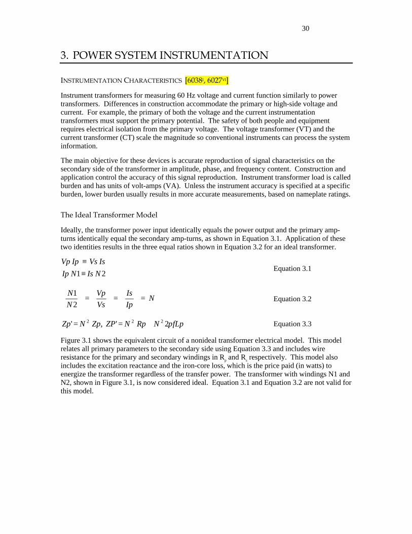
30
3. POWER SYSTEM INSTRUMENTATION
INSTRUMENTATION CHARACTERISTICS [6038I, 6027VI]
Instrument transformers for measuring 60 Hz voltage and current function similarly to power transformers. Differences in construction accommodate the primary or high-side voltage and current. For example, the primary of both the voltage and the current instrumentation transformers must support the primary potential. The safety of both people and equipment requires electrical isolation from the primary voltage. The voltage transformer (VT) and the current transformer (CT) scale the magnitude so conventional instruments can process the system information.
The main objective for these devices is accurate reproduction of signal characteristics on the secondary side of the transformer in amplitude, phase, and frequency content. Construction and application control the accuracy of this signal reproduction. Instrument transformer load is called burden and has units of volt-amps (VA). Unless the instrument accuracy is specified at a specific burden, lower burden usually results in more accurate measurements, based on nameplate ratings.
The Ideal Transformer Model
Ideally, the transformer power input identically equals the power output and the primary amp-turns identically equal the secondary amp-turns, as shown in Equation 3.1. Application of these two identities results in the three equal ratios shown in Equation 3.2 for an ideal transformer.
21 NIsNIp
IsVsIpVp
≡≡
Equation 3.1
NIp
Is
Vs
Vp
N
N=
=
=
2
1 Equation 3.2
fLpNRpNZPZpNZp π2',' 222 +== Equation 3.3
Figure 3.1 shows the equivalent circuit of a nonideal transformer electrical model. This model relates all primary parameters to the secondary side using Equation 3.3 and includes wire resistance for the primary and secondary windings in Rp and Rs respectively. This model also includes the excitation reactance and the iron-core loss, which is the price paid (in watts) to energize the transformer regardless of the transfer power. The transformer with windings N1 and N2, shown in Figure 3.1, is now considered ideal. Equation 3.1 and Equation 3.2 are not valid for this model.
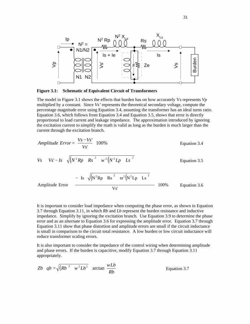
31
XLsN2 Rp Rs
N2 XLp
Ze
Bur
den
Is
Ie
Ip
VsVp
Is + Ie
Vs'
N2 =N1/N2
N1 N2
Figure 3.1: Schematic of Equivalent Circuit of Transformers
The model in Figure 3.1 shows the effects that burden has on how accurately Vs represents Vp multiplied by a constant. Since Vs’ represents the theoretical secondary voltage, compute the percentage magnitude error using Equation 3.4, assuming the transformer has an ideal turns ratio. Equation 3.6, which follows from Equation 3.4 and Equation 3.5, shows that error is directly proportional to load current and leakage impedance. The approximation introduced by ignoring the excitation current to simplify the math is valid as long as the burden is much larger than the current through the excitation branch.
%100'
'
−
=Vs
VsVsErrorAmplitude Equation 3.4
( ) ( )
+++−≅
22222' LsLpNRsRpNIsVsVs ω Equation 3.5
( ) ( )%100
'Vs
LsLpNRsRpNIs
ErrorAmplitude
22222
+ω++−
≅ Equation 3.6
It is important to consider load impedance when computing the phase error, as shown in Equation 3.7 through Equation 3.11, in which Rb and Lb represent the burden resistance and inductive impedance. Simplify by ignoring the excitation branch. Use Equation 3.9 to determine the phase error and as an alternate to Equation 3.6 for expressing the amplitude error. Equation 3.7 through Equation 3.11 show that phase distortion and amplitude errors are small if the circuit inductance is small in comparison to the circuit total resistance. A low burden or low circuit inductance will reduce transformer scaling errors.
It is also important to consider the impedance of the control wiring when determining amplitude and phase errors. If the burden is capacitive, modify Equation 3.7 through Equation 3.11 appropriately.
( )
∠+=∠
Rb
LbLbRbbZb
ωωθ arctan222 Equation 3.7
32
( ) ( )( )
++++ω
∠
++ω+++=θ∠
RbRsRp
LbLsLparctan
LbLsLpRbRsRptZt 222
Equation 3.8
( )tbZt
ZbVssVs θθθ −∠
∠=∠ 0' Equation 3.9
tbserrorPhase θθθ −== Equation 3.10
%1001
−
=
Zt
ZberrorAmplitude Equation 3.11
Polarity
Polarity designations of instrumentation transformers allow proper phasing of voltages and currents. The dots beside the transformer windings in Figure 3.1 denote the polarity terminals and are similarly identified on the physical transformer. Convention dictates that primary current into the polarity terminal induces secondary current out of the polarity terminal. Likewise, a positive voltage presented to the primary polarity terminal produces a positive voltage on the secondary polarity terminal.
CURRENT TRANSFORMERS (CTS)
Design
CTs are used anywhere ac current is measured, on transformer and circuit breaker bushings, on bus bars, on transmission line conductors, and on grounding straps.i They have single (or at most a few) turn(s) primary windings and many secondary windings. A typical rating specifies primary amps to 5 secondary amps, such as 600:5, although other standards are used as well. For instance, instead of a 5-amp secondary rating, use a 2-amp or 1-amp rating. The primary windings must have the capacity to carry the expected current, plus fault current for a short duration.
How are current transformers different from voltage transformers or power transformers? Consider first how CTs connect into the power circuit. As shown in Figure 3.2, the CT is wired in series with the source, line, and load impedances such that the phase current is also the primary CT current. Since the parameter of interest is current, not voltage, the instrumentation must have impedance that is much less than the impedance of the circuit being instrumented. Ideally, current transformers are constant current devices where low leakage impedance is desirable.
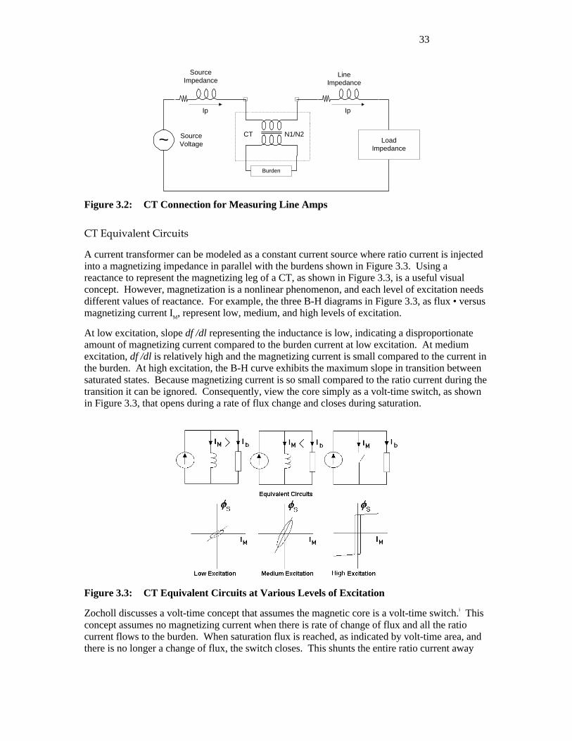
33
N1/N2
Burden
SourceImpedance
IpIp
CT
LineImpedance
~ LoadImpedance
SourceVoltage
Figure 3.2: CT Connection for Measuring Line Amps
CT Equivalent Circuits
A current transformer can be modeled as a constant current source where ratio current is injected into a magnetizing impedance in parallel with the burdens shown in Figure 3.3. Using a reactance to represent the magnetizing leg of a CT, as shown in Figure 3.3, is a useful visual concept. However, magnetization is a nonlinear phenomenon, and each level of excitation needs different values of reactance. For example, the three B-H diagrams in Figure 3.3, as flux • versus magnetizing current IM, represent low, medium, and high levels of excitation.
At low excitation, slope dφ/dl representing the inductance is low, indicating a disproportionate amount of magnetizing current compared to the burden current at low excitation. At medium excitation, dφ/dl is relatively high and the magnetizing current is small compared to the current in the burden. At high excitation, the B-H curve exhibits the maximum slope in transition between saturated states. Because magnetizing current is so small compared to the ratio current during the transition it can be ignored. Consequently, view the core simply as a volt-time switch, as shown in Figure 3.3, that opens during a rate of flux change and closes during saturation.
Figure 3.3: CT Equivalent Circuits at Various Levels of Excitation
Zocholl discusses a volt-time concept that assumes the magnetic core is a volt-time switch.i This concept assumes no magnetizing current when there is rate of change of flux and all the ratio current flows to the burden. When saturation flux is reached, as indicated by volt-time area, and there is no longer a change of flux, the switch closes. This shunts the entire ratio current away
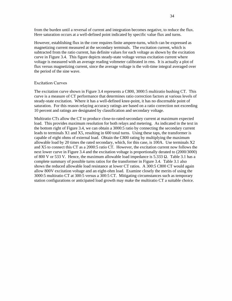
34
from the burden until a reversal of current and integration becomes negative, to reduce the flux. Here saturation occurs at a well-defined point indicated by specific value flux and turns.
However, establishing flux in the core requires finite ampere-turns, which can be expressed as magnetizing current measured at the secondary terminals. The excitation current, which is subtracted from the ratio current, has definite values for each voltage as shown by the excitation curve in Figure 3.4. This figure depicts steady-state voltage versus excitation current where voltage is measured with an average reading voltmeter calibrated in rms. It is actually a plot of flux versus magnetizing current, since the average voltage is the volt-time integral averaged over the period of the sine wave.
Excitation Curves
The excitation curve shown in Figure 3.4 represents a C800, 3000:5 multiratio bushing CT. This curve is a measure of CT performance that determines ratio correction factors at various levels of steady-state excitation. Where it has a well-defined knee-point, it has no discernable point of saturation. For this reason relaying accuracy ratings are based on a ratio correction not exceeding 10 percent and ratings are designated by classification and secondary voltage.
Multiratio CTs allow the CT to produce close-to-rated-secondary current at maximum expected load. This provides maximum resolution for both relays and metering. As indicated in the text in the bottom right of Figure 3.4, we can obtain a 3000:5 ratio by connecting the secondary current leads to terminals X1 and X5, resulting in 600 total turns. Using these taps, the transformer is capable of eight ohms of external load. Obtain the C800 rating by multiplying the maximum allowable load by 20 times the rated secondary, which, for this case, is 100A. Use terminals X2 and X5 to connect this CT as a 2000:5 ratio CT. However, the excitation current now follows the next lower curve in Figure 3.4 and the excitation voltage is proportionally derated to (2000/3000) of 800 V or 533 V. Hence, the maximum allowable load impedance is 5.333 Ω. Table 3.1 has a complete summary of possible turns ratios for the transformer in Figure 3.4. Table 3.1 also shows the reduced allowable load resistance at lower CT ratios. A 300:5 C800 CT would again allow 800V excitation voltage and an eight-ohm load. Examine closely the merits of using the 3000:5 multiratio CT at 300:5 versus a 300:5 CT. Mitigating circumstances such as temporary station configurations or anticipated load growth may make the multiratio CT a suitable choice.
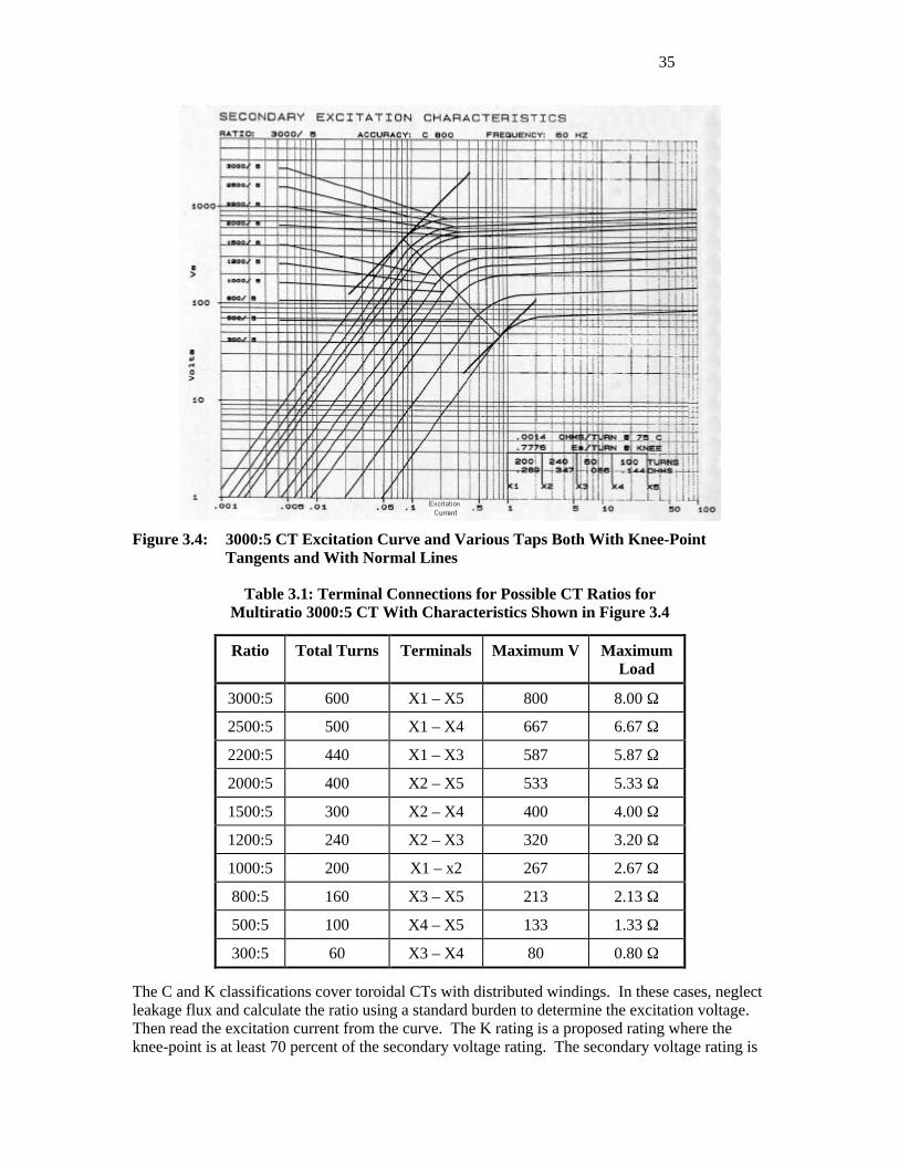
35
Figure 3.4: 3000:5 CT Excitation Curve and Various Taps Both With Knee-Point Tangents and With Normal Lines
Table 3.1: Terminal Connections for Possible CT Ratios for Multiratio 3000:5 CT With Characteristics Shown in Figure 3.4
Ratio Total Turns Terminals Maximum V Maximum Load
3000:5 600 X1 – X5 800 8.00 Ω
2500:5 500 X1 – X4 667 6.67 Ω
2200:5 440 X1 – X3 587 5.87 Ω
2000:5 400 X2 – X5 533 5.33 Ω
1500:5 300 X2 – X4 400 4.00 Ω
1200:5 240 X2 – X3 320 3.20 Ω
1000:5 200 X1 – x2 267 2.67 Ω
800:5 160 X3 – X5 213 2.13 Ω
500:5 100 X4 – X5 133 1.33 Ω
300:5 60 X3 – X4 80 0.80 Ω
The C and K classifications cover toroidal CTs with distributed windings. In these cases, neglect leakage flux and calculate the ratio using a standard burden to determine the excitation voltage. Then read the excitation current from the curve. The K rating is a proposed rating where the knee-point is at least 70 percent of the secondary voltage rating. The secondary voltage rating is

36
the voltage the CT will deliver to a standard burden at 20 times rated secondary current without exceeding 10 percent ratio correction. The standard burden values for relaying are 1.0, 2.0, 4.0, and 8.0 ohms, all with an impedance angle of 60°. Consequently, at 20 times the rated current of 5 amperes the standard voltage ratings are 100, 200, 400, and 800 volts. Use standard burden values of 0.1, 0.2, and 0.5, with a 25.8° impedance angle, for rating metering CTs that are of insufficient accuracy for relaying.
A multiratio CT is voltage rated using the maximum turns ratio. The voltage read from the upper curve at 10 amps excitation current is 486 volts. This is less than the standard rating of C800 but above C400. Accordingly, the CT is rated C400. Calculate the magnetizing impedance of the CT by dividing each value of voltage read from the curve by the corresponding excitation current. The results are shown in Table 1. The magnetizing impedance is nonlinear, increasing from 1200 ohms at 0.001 amps excitation current to a maximum of 5625 ohms at 0.08 amperes of excitation. This is the point of maximum permeability and is located by the 45° tangent to the curve. The impedance values decrease from this point because the excitation is increased, reaching 90 ohms at 10 amperes of excitation current.
Table 3.2: Excitation Curve Values for the CT Characteristics of Figure 3.4
V(volts) Ie(amperes) Ze(ohms)
1.2 0.001 1200
3.0 0.002 1500
5.0 0.003 1667
10 0.004 2500
29 0.010 2900
70 0.020 3500
250 0.050 5000
450 0.080 5625
530 0.100 5300
720 0.200 3600
800 1.000 800
830 4.000 207
870 6.000 145
900 10.00 90
Refer any point on the maximum ratio curve to a lower ratio tap by using a constant volts-per-turn relation for the voltage and a constant ampere-turn relation for the current. Consequently:
IN
N=I VN
N=V 12
121
1
22 Equation 3.12
so that the knee-point of each curve lies along the normal line to the 45° tangent drawn in Figure 3.4. Figure 3.4 also shows the curve for the 300:5 ampere minimum tap.
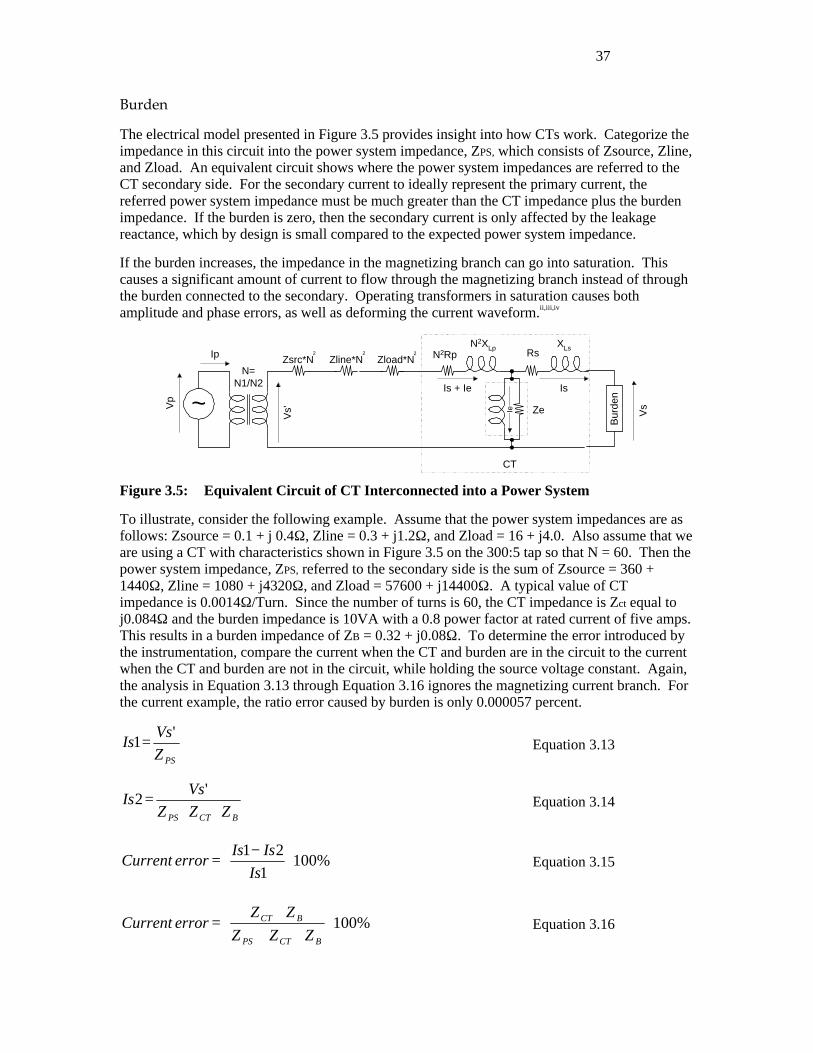
37
Burden
The electrical model presented in Figure 3.5 provides insight into how CTs work. Categorize the impedance in this circuit into the power system impedance, ZPS, which consists of Zsource, Zline, and Zload. An equivalent circuit shows where the power system impedances are referred to the CT secondary side. For the secondary current to ideally represent the primary current, the referred power system impedance must be much greater than the CT impedance plus the burden impedance. If the burden is zero, then the secondary current is only affected by the leakage reactance, which by design is small compared to the expected power system impedance.
If the burden increases, the impedance in the magnetizing branch can go into saturation. This causes a significant amount of current to flow through the magnetizing branch instead of through the burden connected to the secondary. Operating transformers in saturation causes both amplitude and phase errors, as well as deforming the current waveform.ii,iii,iv
~
N=N1/N2
Ip
VsV
p
Zsrc*N2
Zline*N2
Zload*N2 N2Rp Rs
Ze
Bur
den
Is
Ie
Is + Ie
Vs'
XLsN2XLp
CT
Figure 3.5: Equivalent Circuit of CT Interconnected into a Power System
To illustrate, consider the following example. Assume that the power system impedances are as follows: Zsource = 0.1 + j 0.4Ω, Zline = 0.3 + j1.2Ω, and Zload = 16 + j4.0. Also assume that we are using a CT with characteristics shown in Figure 3.5 on the 300:5 tap so that N = 60. Then the power system impedance, ZPS, referred to the secondary side is the sum of Zsource = 360 + 1440Ω, Zline = 1080 + j4320Ω, and Zload = 57600 + j14400Ω. A typical value of CT impedance is 0.0014Ω/Turn. Since the number of turns is 60, the CT impedance is Zct equal to j0.084Ω and the burden impedance is 10VA with a 0.8 power factor at rated current of five amps. This results in a burden impedance of ZB = 0.32 + j0.08Ω. To determine the error introduced by the instrumentation, compare the current when the CT and burden are in the circuit to the current when the CT and burden are not in the circuit, while holding the source voltage constant. Again, the analysis in Equation 3.13 through Equation 3.16 ignores the magnetizing current branch. For the current example, the ratio error caused by burden is only 0.000057 percent.
PSZ
VsIs
'1= Equation 3.13
BCTPS ZZZ
VsIs
++=
'2 Equation 3.14
%1001
21
−=
Is
IsIserrorCurrent Equation 3.15
%100
++
+=
BCTPS
BCT
ZZZ
ZZerrorCurrent Equation 3.16
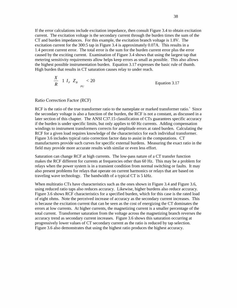
38
If the error calculations include excitation impedance, then consult Figure 3.4 to obtain excitation current. The excitation voltage is the secondary current through the burden times the sum of the CT and burden impedances. For this example, the excitation branch voltage is 1.8V. The excitation current for the 300:5 tap in Figure 3.4 is approximately 0.07A. This results in a 1.4 percent current error. The total error is the sum for the burden current error plus the error caused by the exciting current. Examination of Figure 3.4 shows that using the largest tap that metering sensitivity requirements allow helps keep errors as small as possible. This also allows the highest possible instrumentation burden. Equation 3.17 expresses the basic rule of thumb. High burden that results in CT saturation causes relay to under reach.
201 <
⋅
+
PU
BF ZIR
X Equation 3.17
Ratio Correction Factor (RCF)
RCF is the ratio of the true transformer ratio to the nameplate or marked transformer ratio.v Since the secondary voltage is also a function of the burden, the RCF is not a constant, as discussed in a later section of this chapter. The ANSI C37.15 classification of CTs guarantees specific accuracy if the burden is under specific limits, but only applies to 60 Hz currents. Adding compensation windings to instrument transformers corrects for amplitude errors at rated burden. Calculating the RCF for a given load requires knowledge of the characteristics for each individual transformer. Figure 3.6 includes typical ratio correction factor data to assist in the computations. CT manufacturers provide such curves for specific external burdens. Measuring the exact ratio in the field may provide more accurate results with similar or even less effort.
Saturation can change RCF at high currents. The low-pass nature of a CT transfer function makes the RCF different for currents at frequencies other than 60 Hz. This may be a problem for relays when the power system is in a transient condition from normal switching or faults. It may also present problems for relays that operate on current harmonics or relays that are based on traveling wave technology. The bandwidth of a typical CT is 5 kHz.
When multiratio CTs have characteristics such as the ones shown in Figure 3.4 and Figure 3.6, using reduced ratio taps also reduces accuracy. Likewise, higher burdens also reduce accuracy. Figure 3.6 shows RCF characteristics for a specified burden, which for this case is the rated load of eight ohms. Note the perceived increase of accuracy as the secondary current increases. This is because the excitation current that can be seen as the cost of energizing the CT dominates the errors at low currents. At higher currents, the magnetizing current is a smaller percentage of the total current. Transformer saturation from the voltage across the magnetizing branch reverses the accuracy trend as secondary current increases. Figure 3.6 shows this saturation occurring at progressively lower values of CT secondary current as the ratio is reduced by tap selection. Figure 3.6 also demonstrates that using the highest ratio produces the highest accuracy.
39
Figure 3.6: Typical Ratio Correction Factor Curves
Angle Correction Factor (ACF)
The transformer burden also affects the phase of the secondary current. Figure 3.5 and Equation 3.18 show this dependency clearly.
++++
−=∠RbRsRp
XLbXLsXLpIs arctan Equation 3.18
where Xlp and Rp are referenced to the transformer secondary side.
Standards
ANSI C37.15, available from IEEE Standards publications, lists the standards for construction and application.
40
Practicesvi
To select the proper CT for an application you must know the application environment and the accuracy required. The application environment includes primary voltage, maximum operating current, maximum fault current, network reactance to resistance ratio, and the instrumentation burden.
Generally, protective relays use fundamental frequency sine waves as inputs and their performance is not specified for other waveforms. Therefore, in a protective relay application, the voltage and burden of the CT should be specified to ensure undistorted secondary current for the maximum fault condition.
IEEE/ANSI Standard C57.13 suggests applying CTs for relaying based on the maximum symmetrical fault current not exceeding 20 times the CT current rating and the burden voltage not exceeding the accuracy class voltage of the CT. There is a rationale for choosing a CT to produce the knee-point on the excitation curve at the maximum symmetrical fault current since the magnetizing reactance is at a maximum. Observe that the knee-point of a typical excitation curve is about 46 percent of excitation voltage corresponding to 10 amperes excitation current. A rule-of-thumb suggests that the C-rating be twice the excitation voltage developed by the maximum fault current, which guarantees operation near the knee-point of the excitation curve for the maximum symmetrical fault.
Preventing saturation from the exponential component of fault current requires a C-rating exceeding the symmetrical rating by a factor equal to the X/R ratio of the faulted primary system plus one. Unfortunately it is routinely impossible to achieve such ratings despite the fact that saturation affects the performance of high-speed relays. In these cases, use simulations to assess the effects of transient saturation on relay performance.
Creating an open-circuit in the CT secondary while connected to an energized power system results in dangerously high potential across the open circuit. The model in Figure 3.2 shows how. The burden impedance reflected back to the primary side is the inverse of the turns ratio squared. If the load resistance is infinite, then the reflected impedance is also infinite regardless of the CT turns ratio. This theoretically causes the primary line-to-ground voltage to drop across the CT primary turns. The voltage is then coupled to the secondary side of the CT that is now operating as a step-up voltage transformer. As a result, the theoretical secondary voltage is the primary line-to-ground voltage divided by the turns ratio. Regardless of the primary voltage, dangerously high potentials can damage personnel and equipment.
Example Calculation of Errors
This example uses the CT curves shown in Figure 3.4 and Figure 3.6 and the circuit shown in Figure 3.5. Equation 3.19 includes the resistance of substation CT wiring with the burden resistance. As shown in the previous sections, the CT burden consists of internal burden, the CT impedance and external burden, and the impedance of the devices connected to the CT, plus the substation CT wiring resistance.
.1000/32.2232.0 fteRw G Ω= −⋅ Equation 3.19
where G is AWG wire gauge.
The data in the lower right of Figure 3.4 shows that the CT secondary winding resistance is 0.0014 Ω per turn. Therefore, the greater the turns ratio, the greater the total resistance. We now
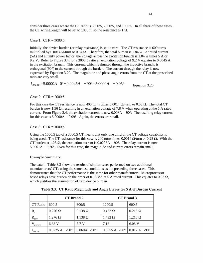
41
consider three cases where the CT ratio is 3000:5, 2000:5, and 1000:5. In all three of these cases, the CT wiring length will be set to 1000 ft, so the resistance is 1 Ω.
Case 1: CTR = 3000:5
Initially, the device burden (or relay resistance) is set to zero. The CT resistance is 600 turns multiplied by 0.0014 Ω/turn or 0.84 Ω. Therefore, the total burden is 1.84 Ω. At rated current (5A) and at unity power factor, the voltage across the excitation branch is 1.84 Ω times 5 A or 9.2 V. Refer to Figure 3.4; for a 3000:5 ratio an excitation voltage of 9.2 V equates to 0.0045 A in the excitation branch. This current, which is shunted through the inductive branch, is orthogonal (90°) to the current through the burden. The current through the relay is now expressed by Equation 3.20. The magnitude and phase angle errors from the CT at the prescribed ratio are very small.
°−∠=°−∠−°∠= 05.00000.5900045.000000.5 AAAI RELAY Equation 3.20
Case 2: CTR = 2000:5
For this case the CT resistance is now 400 turns times 0.0014 Ω/turn, or 0.56 Ω. The total CT burden is now 1.56 Ω, resulting in an excitation voltage of 7.8 V when operating at the 5 A rated current. From Figure 3.4, the excitation current is now 0.008A∠-90°. The resulting relay current for this case is 5.0000A∠-0.09°. Again, the errors are small.
Case 3: CTR = 1000:5
Using the 1000:5 tap of a 3000:5 CT means that only one third of the CT voltage capability is being used. The CT resistance for this case is 200 turns times 0.0014 Ω/turn or 0.28 Ω. With the CT burden at 1.28 Ω, the excitation current is 0.0225A∠-90°. The relay current is now 5.0001A∠-0.26°. Even for this case, the magnitude and current errors remain small.
Example Summary
The data in Table 3.3 show the results of similar cases performed on two additional manufacturers’ CTs using the same test conditions as the preceding three cases. This demonstrates that the CT performance is the same for other manufacturers. Microprocessor-based relays have burden on the order of 0.15 VA at 5 A rated current. This equates to 0.03 Ω, which justifies the assumption of zero device burden.
Table 3.3: CT Ratio Magnitude and Angle Errors for 5 A of Burden Current
CT Brand 2 CT Brand 3
CT Ratio 600:5 300:5 1200:5 600:5
RCT 0.276 Ω 0.138 Ω 0.432 Ω 0.216 Ω
RTOT 1.276 Ω 1.138 Ω 1.432 Ω 1.216 Ω
VEXCITE 6.38 V 5.7 V 7.16 6.08 V
IEXCITE 0.0225 A ∠-90° 0.060A∠-90° 0.0055 A∠-90° 0.017 A∠-90°
42
IRELAY 5.0001 A ∠-0.258°
5.0040 A ∠-0.69°
5.0000 A ∠-0.063°
5.0000 A ∠-0.195°
POTENTIAL MEASURING DEVICES
Numerous instruments can measure the primary circuit voltage. Cost, accuracy, and application voltages vary to meet the requirements of the application account. Conventionally, the secondary voltage for power system voltage transformers is 120 Vac phase-to-phase or 69.3 Vac phase-to-ground.
VT
Voltage transformer (VT) devices are usually more accurate than other conventional potential measuring devices. VT devices use wire-wound construction in a similar manner to conventional power transformers with two windings wound around a common iron core. Discussions in the section that discusses operations and errors for current transformers also apply to voltage transformers. The main difference is in what constitutes burden. Although high load impedance constitutes a high burden for CTs, the opposite is true for VTs, which are constant voltage devices where it is desirable to have minimal magnetizing current.
For VTs, power can flow from the primary side or the secondary side. It is possible to generate, either intentionally or unintentionally, primary voltages by energizing VTs from the secondary side. If the VTs are installed in a substation, it is possible to energize portions of the substation by this back-feeding phenomenon.
CCVT
Capacitor-coupled voltage transformers use a capacitive voltage divider and a low voltage transformer for impedance matching as shown in Figure 3.7. These devices can also couple high frequency RF signals to the power line for communication.
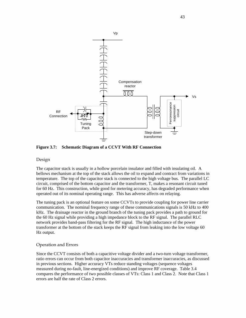
43
RFConnection
TuningPack
Vp
Vs
Fer
rore
sona
nce
supp
ress
ion
circ
uit
Step-downtransformer
Compensationreactor
Figure 3.7: Schematic Diagram of a CCVT With RF Connection
Design
The capacitor stack is usually in a hollow porcelain insulator and filled with insulating oil. A bellows mechanism at the top of the stack allows the oil to expand and contract from variations in temperature. The top of the capacitor stack is connected to the high voltage bus. The parallel LC circuit, comprised of the bottom capacitor and the transformer, T, makes a resonant circuit tuned for 60 Hz. This construction, while good for metering accuracy, has degraded performance when operated out of its nominal operating range. This has adverse affects on relaying.
The tuning pack is an optional feature on some CCVTs to provide coupling for power line carrier communication. The nominal frequency range of these communications signals is 50 kHz to 400 kHz. The drainage reactor in the ground branch of the tuning pack provides a path to ground for the 60 Hz signal while providing a high impedance block to the RF signal. The parallel RLC network provides band-pass filtering for the RF signal. The high inductance of the power transformer at the bottom of the stack keeps the RF signal from leaking into the low voltage 60 Hz output.
Operation and Errors
Since the CCVT consists of both a capacitive voltage divider and a two-turn voltage transformer, ratio errors can occur from both capacitor inaccuracies and transformer inaccuracies, as discussed in previous sections. Higher accuracy VTs reduce standing voltages (sequence voltages measured during no-fault, line-energized conditions) and improve RF coverage. Table 3.4 compares the performance of two possible classes of VTs: Class 1 and Class 2. Note that Class 1 errors are half the rate of Class 2 errors.
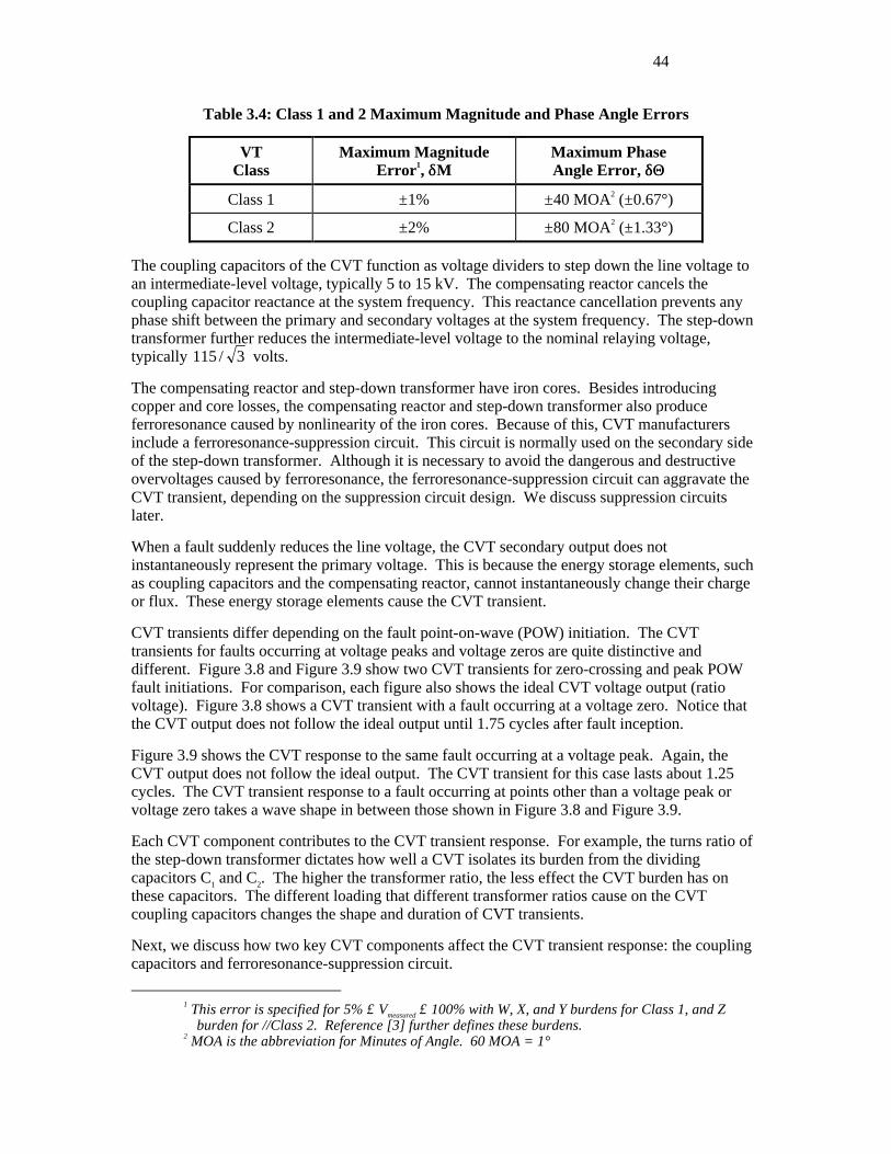
44
Table 3.4: Class 1 and 2 Maximum Magnitude and Phase Angle Errors
VT Class
Maximum Magnitude Error1, δδM
Maximum Phase Angle Error, δδΘΘ
Class 1 ±1% ±40 MOA2 (±0.67°)
Class 2 ±2% ±80 MOA2 (±1.33°)
The coupling capacitors of the CVT function as voltage dividers to step down the line voltage to an intermediate-level voltage, typically 5 to 15 kV. The compensating reactor cancels the coupling capacitor reactance at the system frequency. This reactance cancellation prevents any phase shift between the primary and secondary voltages at the system frequency. The step-down transformer further reduces the intermediate-level voltage to the nominal relaying voltage, typically 3/115 volts.
The compensating reactor and step-down transformer have iron cores. Besides introducing copper and core losses, the compensating reactor and step-down transformer also produce ferroresonance caused by nonlinearity of the iron cores. Because of this, CVT manufacturers include a ferroresonance-suppression circuit. This circuit is normally used on the secondary side of the step-down transformer. Although it is necessary to avoid the dangerous and destructive overvoltages caused by ferroresonance, the ferroresonance-suppression circuit can aggravate the CVT transient, depending on the suppression circuit design. We discuss suppression circuits later.
When a fault suddenly reduces the line voltage, the CVT secondary output does not instantaneously represent the primary voltage. This is because the energy storage elements, such as coupling capacitors and the compensating reactor, cannot instantaneously change their charge or flux. These energy storage elements cause the CVT transient.
CVT transients differ depending on the fault point-on-wave (POW) initiation. The CVT transients for faults occurring at voltage peaks and voltage zeros are quite distinctive and different. Figure 3.8 and Figure 3.9 show two CVT transients for zero-crossing and peak POW fault initiations. For comparison, each figure also shows the ideal CVT voltage output (ratio voltage). Figure 3.8 shows a CVT transient with a fault occurring at a voltage zero. Notice that the CVT output does not follow the ideal output until 1.75 cycles after fault inception.
Figure 3.9 shows the CVT response to the same fault occurring at a voltage peak. Again, the CVT output does not follow the ideal output. The CVT transient for this case lasts about 1.25 cycles. The CVT transient response to a fault occurring at points other than a voltage peak or voltage zero takes a wave shape in between those shown in Figure 3.8 and Figure 3.9.
Each CVT component contributes to the CVT transient response. For example, the turns ratio of the step-down transformer dictates how well a CVT isolates its burden from the dividing capacitors C1 and C2. The higher the transformer ratio, the less effect the CVT burden has on these capacitors. The different loading that different transformer ratios cause on the CVT coupling capacitors changes the shape and duration of CVT transients.
Next, we discuss how two key CVT components affect the CVT transient response: the coupling capacitors and ferroresonance-suppression circuit.
1 This error is specified for 5% ≤ Vmeasured ≤ 100% with W, X, and Y burdens for Class 1, and Z
burden for //Class 2. Reference [3] further defines these burdens. 2 MOA is the abbreviation for Minutes of Angle. 60 MOA = 1°
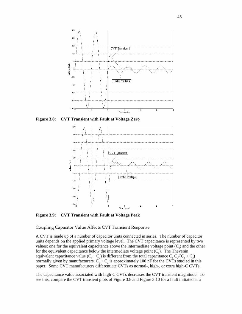
45
Figure 3.8: CVT Transient with Fault at Voltage Zero
Figure 3.9: CVT Transient with Fault at Voltage Peak
Coupling Capacitor Value Affects CVT Transient Response
A CVT is made up of a number of capacitor units connected in series. The number of capacitor units depends on the applied primary voltage level. The CVT capacitance is represented by two values: one for the equivalent capacitance above the intermediate voltage point (C1) and the other for the equivalent capacitance below the intermediate voltage point (C2). The Thevenin equivalent capacitance value (C1 + C2) is different from the total capacitance C1⋅C2/(C1 + C2) normally given by manufacturers. C1 + C2 is approximately 100 nF for the CVTs studied in this paper. Some CVT manufacturers differentiate CVTs as normal-, high-, or extra high-C CVTs.
The capacitance value associated with high-C CVTs decreases the CVT transient magnitude. To see this, compare the CVT transient plots of Figure 3.8 and Figure 3.10 for a fault initiated at a
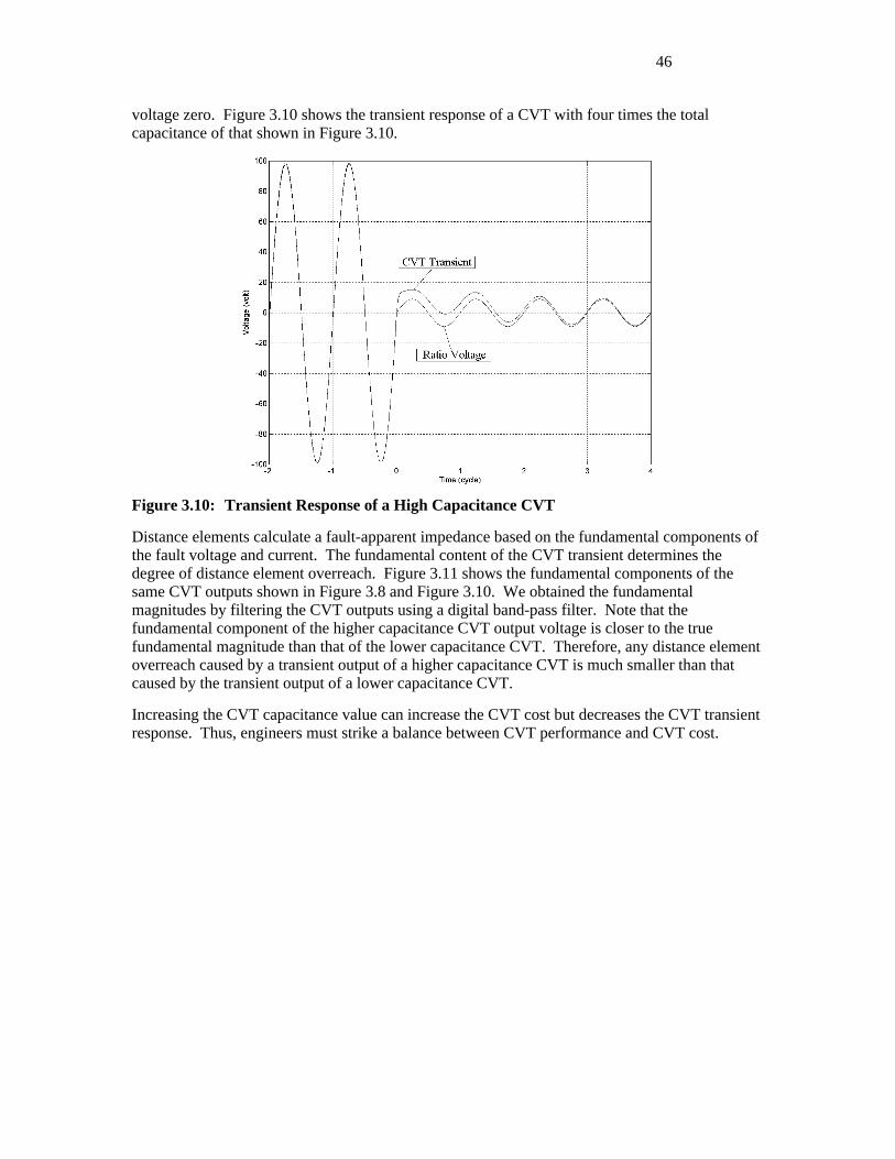
46
voltage zero. Figure 3.10 shows the transient response of a CVT with four times the total capacitance of that shown in Figure 3.10.
Figure 3.10: Transient Response of a High Capacitance CVT
Distance elements calculate a fault-apparent impedance based on the fundamental components of the fault voltage and current. The fundamental content of the CVT transient determines the degree of distance element overreach. Figure 3.11 shows the fundamental components of the same CVT outputs shown in Figure 3.8 and Figure 3.10. We obtained the fundamental magnitudes by filtering the CVT outputs using a digital band-pass filter. Note that the fundamental component of the higher capacitance CVT output voltage is closer to the true fundamental magnitude than that of the lower capacitance CVT. Therefore, any distance element overreach caused by a transient output of a higher capacitance CVT is much smaller than that caused by the transient output of a lower capacitance CVT.
Increasing the CVT capacitance value can increase the CVT cost but decreases the CVT transient response. Thus, engineers must strike a balance between CVT performance and CVT cost.
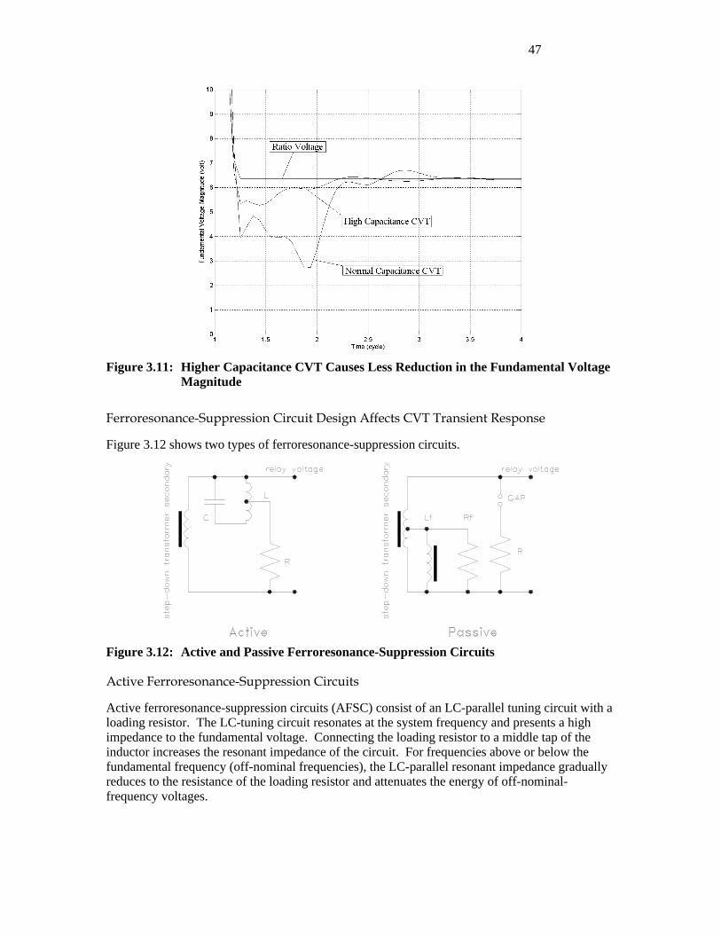
47
Figure 3.11: Higher Capacitance CVT Causes Less Reduction in the Fundamental Voltage Magnitude
Ferroresonance-Suppression Circuit Design Affects CVT Transient Response
Figure 3.12 shows two types of ferroresonance-suppression circuits.
Figure 3.12: Active and Passive Ferroresonance-Suppression Circuits
Active Ferroresonance-Suppression Circuits
Active ferroresonance-suppression circuits (AFSC) consist of an LC-parallel tuning circuit with a loading resistor. The LC-tuning circuit resonates at the system frequency and presents a high impedance to the fundamental voltage. Connecting the loading resistor to a middle tap of the inductor increases the resonant impedance of the circuit. For frequencies above or below the fundamental frequency (off-nominal frequencies), the LC-parallel resonant impedance gradually reduces to the resistance of the loading resistor and attenuates the energy of off-nominal-frequency voltages.
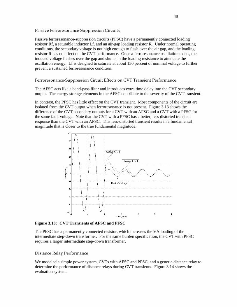
48
Passive Ferroresonance-Suppression Circuits
Passive ferroresonance-suppression circuits (PFSC) have a permanently connected loading resistor Rf, a saturable inductor Lf, and an air-gap loading resistor R. Under normal operating conditions, the secondary voltage is not high enough to flash over the air gap, and the loading resistor R has no effect on the CVT performance. Once a ferroresonance oscillation exists, the induced voltage flashes over the gap and shunts in the loading resistance to attenuate the oscillation energy. Lf is designed to saturate at about 150 percent of nominal voltage to further prevent a sustained ferroresonance condition.
Ferroresonance-Suppression Circuit Effects on CVT Transient Performance
The AFSC acts like a band-pass filter and introduces extra time delay into the CVT secondary output. The energy storage elements in the AFSC contribute to the severity of the CVT transient.
In contrast, the PFSC has little effect on the CVT transient. Most components of the circuit are isolated from the CVT output when ferroresonance is not present. Figure 3.13 shows the difference of the CVT secondary outputs for a CVT with an AFSC and a CVT with a PFSC for the same fault voltage. Note that the CVT with a PFSC has a better, less distorted transient response than the CVT with an AFSC. This less-distorted transient results in a fundamental magnitude that is closer to the true fundamental magnitude..
Figure 3.13: CVT Transients of AFSC and PFSC
The PFSC has a permanently connected resistor, which increases the VA loading of the intermediate step-down transformer. For the same burden specification, the CVT with PFSC requires a larger intermediate step-down transformer.
Distance Relay Performance
We modeled a simple power system, CVTs with AFSC and PFSC, and a generic distance relay to determine the performance of distance relays during CVT transients. Figure 3.14 shows the evaluation system.
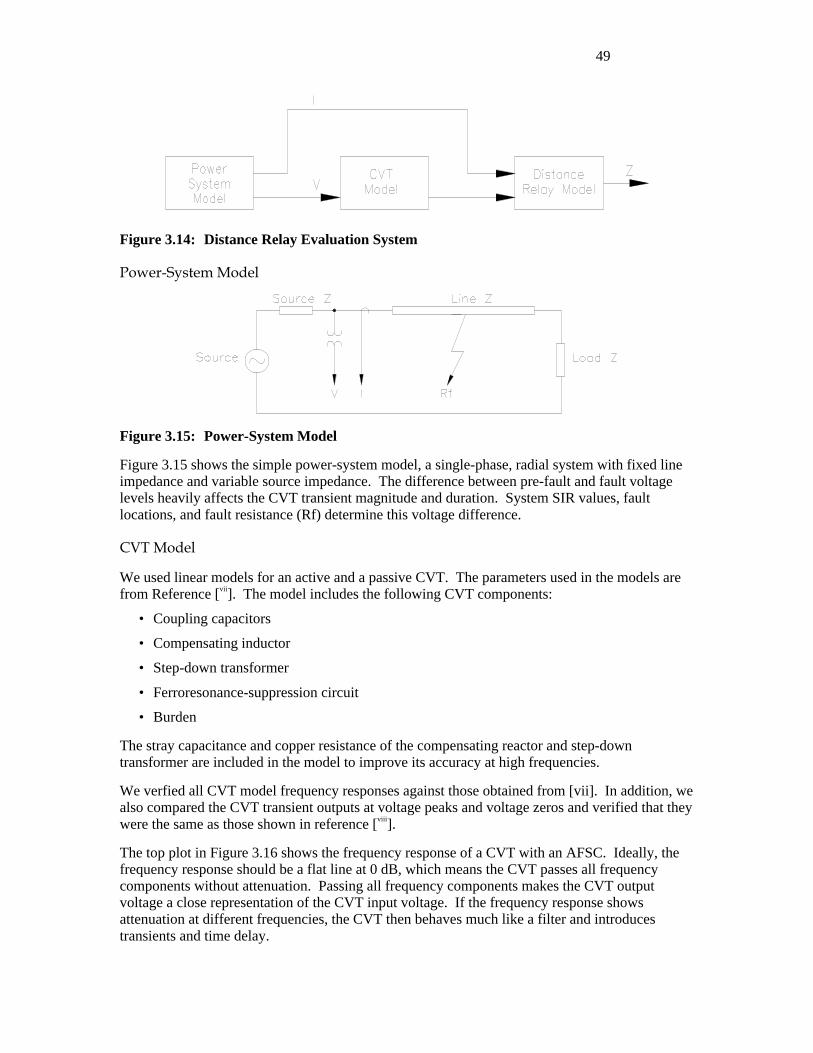
49
Figure 3.14: Distance Relay Evaluation System
Power-System Model
Figure 3.15: Power-System Model
Figure 3.15 shows the simple power-system model, a single-phase, radial system with fixed line impedance and variable source impedance. The difference between pre-fault and fault voltage levels heavily affects the CVT transient magnitude and duration. System SIR values, fault locations, and fault resistance (Rf) determine this voltage difference.
CVT Model
We used linear models for an active and a passive CVT. The parameters used in the models are from Reference [vii]. The model includes the following CVT components:
• Coupling capacitors
• Compensating inductor
• Step-down transformer
• Ferroresonance-suppression circuit
• Burden
The stray capacitance and copper resistance of the compensating reactor and step-down transformer are included in the model to improve its accuracy at high frequencies.
We verfied all CVT model frequency responses against those obtained from [vii]. In addition, we also compared the CVT transient outputs at voltage peaks and voltage zeros and verified that they were the same as those shown in reference [viii].
The top plot in Figure 3.16 shows the frequency response of a CVT with an AFSC. Ideally, the frequency response should be a flat line at 0 dB, which means the CVT passes all frequency components without attenuation. Passing all frequency components makes the CVT output voltage a close representation of the CVT input voltage. If the frequency response shows attenuation at different frequencies, the CVT then behaves much like a filter and introduces transients and time delay.
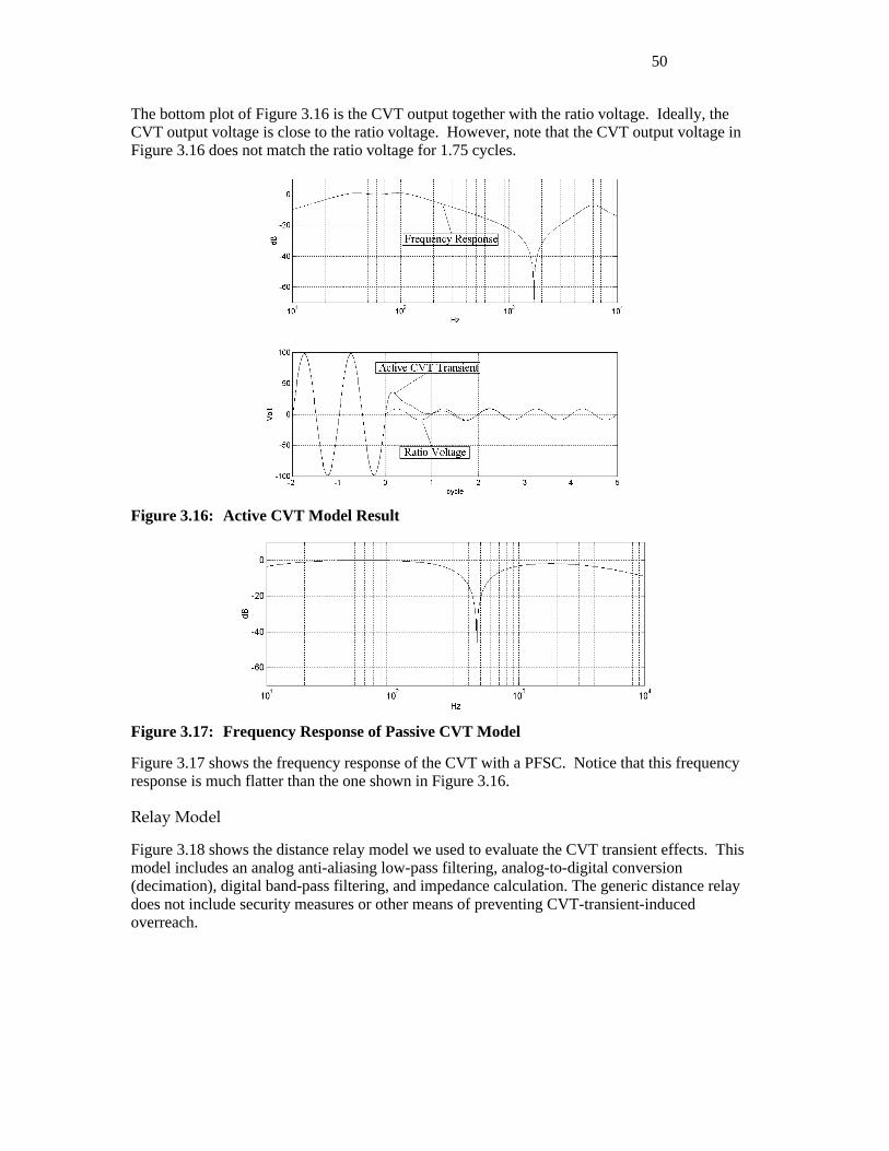
50
The bottom plot of Figure 3.16 is the CVT output together with the ratio voltage. Ideally, the CVT output voltage is close to the ratio voltage. However, note that the CVT output voltage in Figure 3.16 does not match the ratio voltage for 1.75 cycles.
Figure 3.16: Active CVT Model Result
Figure 3.17: Frequency Response of Passive CVT Model
Figure 3.17 shows the frequency response of the CVT with a PFSC. Notice that this frequency response is much flatter than the one shown in Figure 3.16.
Relay Model
Figure 3.18 shows the distance relay model we used to evaluate the CVT transient effects. This model includes an analog anti-aliasing low-pass filtering, analog-to-digital conversion (decimation), digital band-pass filtering, and impedance calculation. The generic distance relay does not include security measures or other means of preventing CVT-transient-induced overreach.
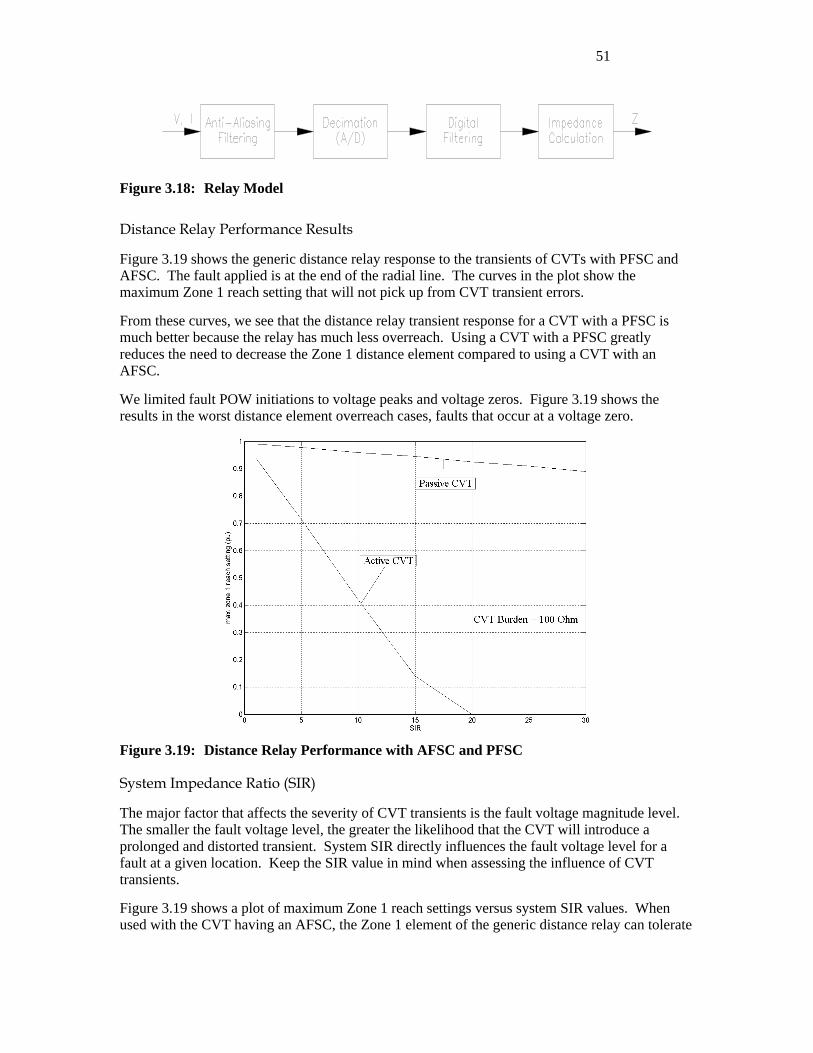
51
Figure 3.18: Relay Model
Distance Relay Performance Results
Figure 3.19 shows the generic distance relay response to the transients of CVTs with PFSC and AFSC. The fault applied is at the end of the radial line. The curves in the plot show the maximum Zone 1 reach setting that will not pick up from CVT transient errors.
From these curves, we see that the distance relay transient response for a CVT with a PFSC is much better because the relay has much less overreach. Using a CVT with a PFSC greatly reduces the need to decrease the Zone 1 distance element compared to using a CVT with an AFSC.
We limited fault POW initiations to voltage peaks and voltage zeros. Figure 3.19 shows the results in the worst distance element overreach cases, faults that occur at a voltage zero.
Figure 3.19: Distance Relay Performance with AFSC and PFSC
System Impedance Ratio (SIR)
The major factor that affects the severity of CVT transients is the fault voltage magnitude level. The smaller the fault voltage level, the greater the likelihood that the CVT will introduce a prolonged and distorted transient. System SIR directly influences the fault voltage level for a fault at a given location. Keep the SIR value in mind when assessing the influence of CVT transients.
Figure 3.19 shows a plot of maximum Zone 1 reach settings versus system SIR values. When used with the CVT having an AFSC, the Zone 1 element of the generic distance relay can tolerate
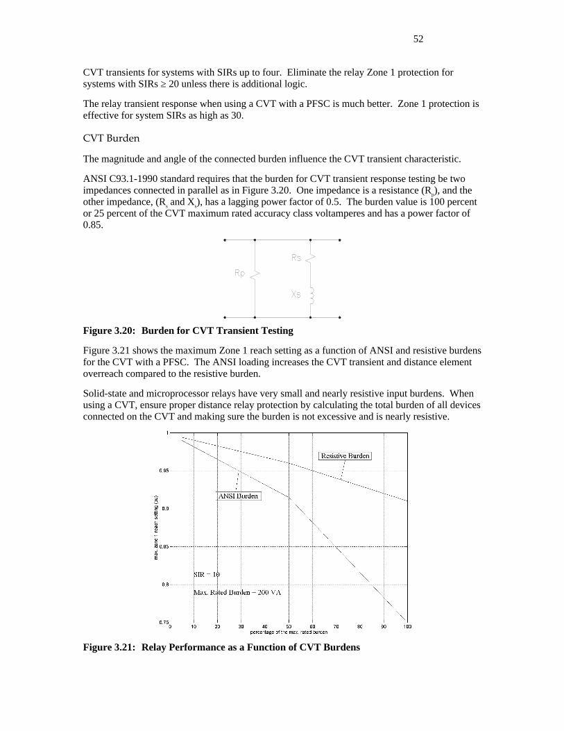
52
CVT transients for systems with SIRs up to four. Eliminate the relay Zone 1 protection for systems with SIRs ≥ 20 unless there is additional logic.
The relay transient response when using a CVT with a PFSC is much better. Zone 1 protection is effective for system SIRs as high as 30.
CVT Burden
The magnitude and angle of the connected burden influence the CVT transient characteristic.
ANSI C93.1-1990 standard requires that the burden for CVT transient response testing be two impedances connected in parallel as in Figure 3.20. One impedance is a resistance (Rp), and the other impedance, (Rs and Xs), has a lagging power factor of 0.5. The burden value is 100 percent or 25 percent of the CVT maximum rated accuracy class voltamperes and has a power factor of 0.85.
Figure 3.20: Burden for CVT Transient Testing
Figure 3.21 shows the maximum Zone 1 reach setting as a function of ANSI and resistive burdens for the CVT with a PFSC. The ANSI loading increases the CVT transient and distance element overreach compared to the resistive burden.
Solid-state and microprocessor relays have very small and nearly resistive input burdens. When using a CVT, ensure proper distance relay protection by calculating the total burden of all devices connected on the CVT and making sure the burden is not excessive and is nearly resistive.
Figure 3.21: Relay Performance as a Function of CVT Burdens
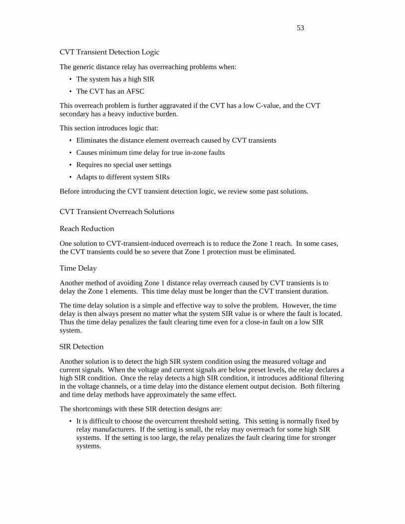
53
CVT Transient Detection Logic
The generic distance relay has overreaching problems when:
• The system has a high SIR
• The CVT has an AFSC
This overreach problem is further aggravated if the CVT has a low C-value, and the CVT secondary has a heavy inductive burden.
This section introduces logic that:
• Eliminates the distance element overreach caused by CVT transients
• Causes minimum time delay for true in-zone faults
• Requires no special user settings
• Adapts to different system SIRs
Before introducing the CVT transient detection logic, we review some past solutions.
CVT Transient Overreach Solutions
Reach Reduction
One solution to CVT-transient-induced overreach is to reduce the Zone 1 reach. In some cases, the CVT transients could be so severe that Zone 1 protection must be eliminated.
Time Delay
Another method of avoiding Zone 1 distance relay overreach caused by CVT transients is to delay the Zone 1 elements. This time delay must be longer than the CVT transient duration.
The time delay solution is a simple and effective way to solve the problem. However, the time delay is then always present no matter what the system SIR value is or where the fault is located. Thus the time delay penalizes the fault clearing time even for a close-in fault on a low SIR system.
SIR Detection
Another solution is to detect the high SIR system condition using the measured voltage and current signals. When the voltage and current signals are below preset levels, the relay declares a high SIR condition. Once the relay detects a high SIR condition, it introduces additional filtering in the voltage channels, or a time delay into the distance element output decision. Both filtering and time delay methods have approximately the same effect.
The shortcomings with these SIR detection designs are:
• It is difficult to choose the overcurrent threshold setting. This setting is normally fixed by relay manufacturers. If the setting is small, the relay may overreach for some high SIR systems. If the setting is too large, the relay penalizes the fault clearing time for stronger systems.
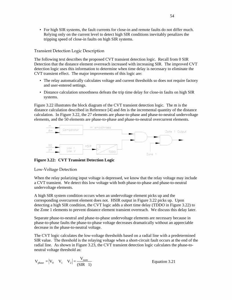
54
• For high SIR systems, the fault currents for close-in and remote faults do not differ much. Relying only on the current level to detect high SIR conditions inevitably penalizes the tripping speed of close-in faults on high SIR systems.
Transient Detection Logic Description
The following text describes the proposed CVT transient detection logic. Recall from 0 SIR Detection that the distance element overreach increased with increasing SIR. The improved CVT detection logic uses this information to determine when time delay is necessary to eliminate the CVT transient effect. The major improvements of this logic are:
• The relay automatically calculates voltage and current thresholds so does not require factory and user-entered settings.
• Distance calculation smoothness defeats the trip time delay for close-in faults on high SIR systems.
Figure 3.22 illustrates the block diagram of the CVT transient detection logic. The m is the distance calculation described in Reference [4] and δm is the incremental quantity of the distance calculation. In Figure 3.22, the 27 elements are phase-to-phase and phase-to-neutral undervoltage elements, and the 50 elements are phase-to-phase and phase-to-neutral overcurrent elements.
Figure 3.22: CVT Transient Detection Logic
Low-Voltage Detection
When the relay polarizing input voltage is depressed, we know that the relay voltage may include a CVT transient. We detect this low voltage with both phase-to-phase and phase-to-neutral undervoltage elements.
A high SIR system condition occurs when an undervoltage element picks up and the corresponding overcurrent element does not. HSIR output in Figure 3.22 picks up. Upon detecting a high SIR condition, the CVT logic adds a short time delay (TDDO in Figure 3.22) to the Zone 1 elements to prevent distance element transient overreach. We discuss this delay later.
Separate phase-to-neutral and phase-to-phase undervoltage elements are necessary because in phase-to-phase faults the phase-to-phase voltage decreases dramatically without an appreciable decrease in the phase-to-neutral voltage.
The CVT logic calculates the low-voltage thresholds based on a radial line with a predetermined SIR value. The threshold is the relaying voltage when a short-circuit fault occurs at the end of the radial line. As shown in Figure 3.23, the CVT transient detection logic calculates the phase-to-neutral voltage threshold as:
1)(SIR
VVVVV nom
210phase +=++= Equation 3.21
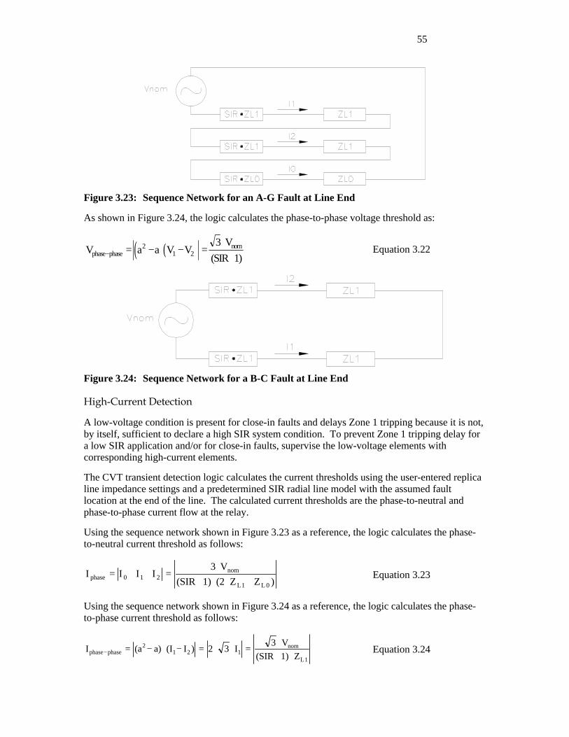
55
Figure 3.23: Sequence Network for an A-G Fault at Line End
As shown in Figure 3.24, the logic calculates the phase-to-phase voltage threshold as:
( ) ( )V3 V
(SIR 1)phase phasenom
− = − ⋅ − =⋅
+a a V V2
1 2 Equation 3.22
Figure 3.24: Sequence Network for a B-C Fault at Line End
High-Current Detection
A low-voltage condition is present for close-in faults and delays Zone 1 tripping because it is not, by itself, sufficient to declare a high SIR system condition. To prevent Zone 1 tripping delay for a low SIR application and/or for close-in faults, supervise the low-voltage elements with corresponding high-current elements.
The CVT transient detection logic calculates the current thresholds using the user-entered replica line impedance settings and a predetermined SIR radial line model with the assumed fault location at the end of the line. The calculated current thresholds are the phase-to-neutral and phase-to-phase current flow at the relay.
Using the sequence network shown in Figure 3.23 as a reference, the logic calculates the phase-to-neutral current threshold as follows:
I I I I3 V
(SIR 1) (2 Z Z )phase 0 1 2nom
L1 L 0
= + + =⋅
+ ⋅ ⋅ + Equation 3.23
Using the sequence network shown in Figure 3.24 as a reference, the logic calculates the phase-to-phase current threshold as follows:
I (a a) (I I ) 2 3 I3 V
(SIR 1) Zphase phase2
1 2 1nom
L1− = − ⋅ − = ⋅ ⋅ =
⋅+ ⋅ Equation 3.24
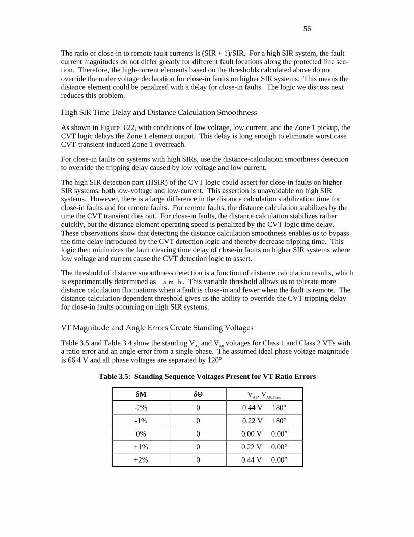
56
The ratio of close-in to remote fault currents is (SIR + 1)/SIR. For a high SIR system, the fault current magnitudes do not differ greatly for different fault locations along the protected line sec-tion. Therefore, the high-current elements based on the thresholds calculated above do not override the under voltage declaration for close-in faults on higher SIR systems. This means the distance element could be penalized with a delay for close-in faults. The logic we discuss next reduces this problem.
High SIR Time Delay and Distance Calculation Smoothness
As shown in Figure 3.22, with conditions of low voltage, low current, and the Zone 1 pickup, the CVT logic delays the Zone 1 element output. This delay is long enough to eliminate worst case CVT-transient-induced Zone 1 overreach.
For close-in faults on systems with high SIRs, use the distance-calculation smoothness detection to override the tripping delay caused by low voltage and low current.
The high SIR detection part (HSIR) of the CVT logic could assert for close-in faults on higher SIR systems, both low-voltage and low-current. This assertion is unavoidable on high SIR systems. However, there is a large difference in the distance calculation stabilization time for close-in faults and for remote faults. For remote faults, the distance calculation stabilizes by the time the CVT transient dies out. For close-in faults, the distance calculation stabilizes rather quickly, but the distance element operating speed is penalized by the CVT logic time delay. These observations show that detecting the distance calculation smoothness enables us to bypass the time delay introduced by the CVT detection logic and thereby decrease tripping time. This logic then minimizes the fault clearing time delay of close-in faults on higher SIR systems where low voltage and current cause the CVT detection logic to assert.
The threshold of distance smoothness detection is a function of distance calculation results, which is experimentally determined as − ⋅ +a m b . This variable threshold allows us to tolerate more distance calculation fluctuations when a fault is close-in and fewer when the fault is remote. The distance calculation-dependent threshold gives us the ability to override the CVT tripping delay for close-in faults occurring on high SIR systems.
VT Magnitude and Angle Errors Create Standing Voltages
Table 3.5 and Table 3.4 show the standing VA2 and VA0 voltages for Class 1 and Class 2 VTs with a ratio error and an angle error from a single phase. The assumed ideal phase voltage magnitude is 66.4 V and all phase voltages are separated by 120°.
Table 3.5: Standing Sequence Voltages Present for VT Ratio Errors
δδM δδΘΘ VA2, VA0, Stand
-2% 0 0.44 V ∠ 180°
-1% 0 0.22 V ∠ 180°
0% 0 0.00 V ∠ 0.00°
+1% 0 0.22 V ∠ 0.00°
+2% 0 0.44 V ∠ 0.00°
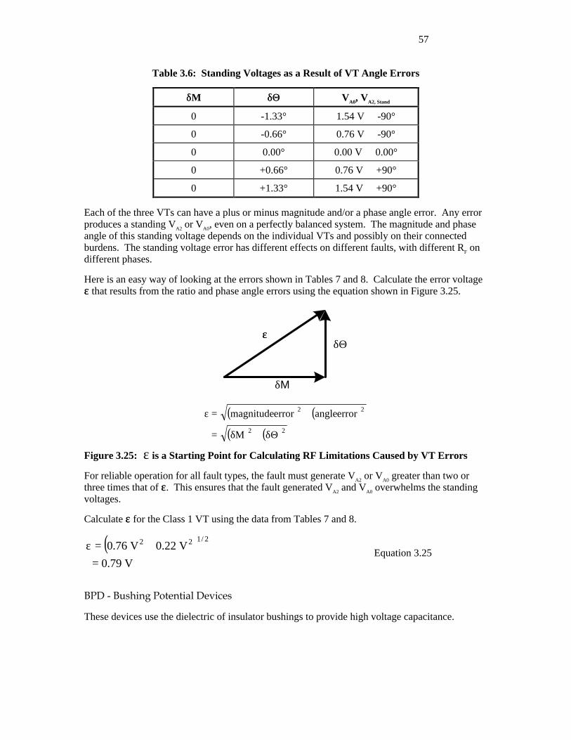
57
Table 3.6: Standing Voltages as a Result of VT Angle Errors
δδM δδΘΘ VA0, VA2, Stand
0 -1.33° 1.54 V ∠ -90°
0 -0.66° 0.76 V ∠ -90°
0 0.00° 0.00 V ∠ 0.00°
0 +0.66° 0.76 V ∠ +90°
0 +1.33° 1.54 V ∠ +90°
Each of the three VTs can have a plus or minus magnitude and/or a phase angle error. Any error produces a standing VA2 or VA0, even on a perfectly balanced system. The magnitude and phase angle of this standing voltage depends on the individual VTs and possibly on their connected burdens. The standing voltage error has different effects on different faults, with different RF on different phases.
Here is an easy way of looking at the errors shown in Tables 7 and 8. Calculate the error voltage εε that results from the ratio and phase angle errors using the equation shown in Figure 3.25.
δM
δΘεε
( ) ( )( ) ( )22
22
M
errorangleerrormagnitude
Θδ+δ=
+=ε
Figure 3.25: ε is a Starting Point for Calculating RF Limitations Caused by VT Errors
For reliable operation for all fault types, the fault must generate VA2 or VA0 greater than two or three times that of εε. This ensures that the fault generated VA2 and VA0 overwhelms the standing voltages.
Calculate εε for the Class 1 VT using the data from Tables 7 and 8.
( )V79.0
V22.0V76.02/122
=+=ε
Equation 3.25
BPD - Bushing Potential Devices
These devices use the dielectric of insulator bushings to provide high voltage capacitance.

58
NONCONVENTIONAL INSTRUMENTATION
Microprocessor-based relaying imposes very low burdens on voltage and current instrumentation. Microprocessor-based relays do not require the high current and high voltage instrumentation needed to operate electromechanical devices. If the burden range is restricted, improved accuracy is possible without increased cost. With lower burdens, new technologies can now be used for instrumentation with wider bandwidth than is needed for traveling wave-based relaying. Minkner and Schweitzer discuss many of these concepts in a 1999 WPRC paper. ix These new technology instruments are also less susceptible to distortions during fault conditions.
Facilities employing both electromechanical and microprocessor-based technologies for metering and relaying are either confined to using the conventional instrumentation discussed above or to installing two sets of instrumentation.
i [6038] S. E. Zocholl and D. W. Smaha, “Current Transformer Concepts”, 19th Annual Western Protective Relay Conference, October 20-22, 1992, Spokane, WA. ii J. R. Lucas, and P.G. McLauren, “Improved Simulation Models for Current and Voltage Transformers in Relay Studies,” IEEE Transactions on Power Delivery, Vol. 7, No. 1, January 1992, pp. 152-159. iii The Relay Performance Considerations with Low-Ratio Current Transformers and High Fault Current Working Group of the IEEE PES Power System Relaying Committee, “Relay Performance Considerations with Low CTS and High Fault Currents”, IEEE Transactions on Power Delivery, Vol. 8, No. 3, July 1993, pp. 884-897. iv W. A. Neves and H. W. Dommel, “On Modeling Iron Core Nonlinearities,” IEEE Transactions on Power Systems, Vol. 8, No. 2, May 1993, pp. 417-425. v Handbook for Electricity Metering-Ninth Edition, Edison Electric Institute, 1992, Edison Electric Institute, Washington, D.C., ISBN 0-931032-30-X. vi [6027] S. E. Zocholl, J. Roberts, and G. Benmouyal, “Selecting CTs to Optimize Relay Performance”, 51st Annual Georgia Tech Protective Relay Conference, Atlanta, GA., April 30-May 2, 1997. vii M. Kezunovic, C. W. Fromen and L. Nilsson, “Digital Models of Coupling Capacitor Voltage Transformers for Protective Relays Transient Studies,” IEEE Transactions on Power Delivery, Vol. 7, No. 4, Oct. 1992. viii A. Sweetana, “Transient Response Characteristics of Capacitive Potential Devices,” IEEE Transactions on Power Aparatus and Systems, Vol. 90, No. 5, Sept./Oct. 1971. ix [6095] I. R. Minkner and E. O. Schweitzer, “Low Power Voltage and Current Transducers for Protecting and Measuring Medium and High Voltage Systems,” 26th Annual Western Protective Relay Conference, Spokane WA, Oct. 26-28, 1999.
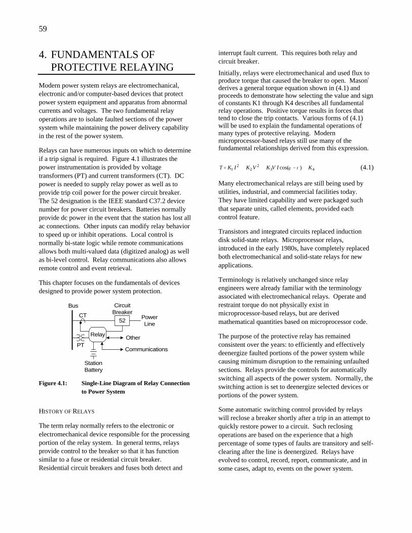
59
4. FUNDAMENTALS OF PROTECTIVE RELAYING
Modern power system relays are electromechanical, electronic and/or computer-based devices that protect power system equipment and apparatus from abnormal currents and voltages. The two fundamental relay operations are to isolate faulted sections of the power system while maintaining the power delivery capability in the rest of the power system.
Relays can have numerous inputs on which to determine if a trip signal is required. Figure 4.1 illustrates the power instrumentation is provided by voltage transformers (PT) and current transformers (CT). DC power is needed to supply relay power as well as to provide trip coil power for the power circuit breaker. The 52 designation is the IEEE standard C37.2 device number for power circuit breakers. Batteries normally provide dc power in the event that the station has lost all ac connections. Other inputs can modify relay behavior to speed up or inhibit operations. Local control is normally bi-state logic while remote communications allows both multi-valued data (digitized analog) as well as bi-level control. Relay communications also allows remote control and event retrieval.
This chapter focuses on the fundamentals of devices designed to provide power system protection.
52
PT
CT
Bus
OtherRelay
Communications
StationBattery
CircuitBreaker
PowerLine
Figure 4.1: Single-Line Diagram of Relay Connection to Power System
HISTORY OF RELAYS
The term relay normally refers to the electronic or electromechanical device responsible for the processing portion of the relay system. In general terms, relays provide control to the breaker so that it has function similar to a fuse or residential circuit breaker. Residential circuit breakers and fuses both detect and
interrupt fault current. This requires both relay and circuit breaker.
Initially, relays were electromechanical and used flux to produce torque that caused the breaker to open. Masoni derives a general torque equation shown in (4.1) and proceeds to demonstrate how selecting the value and sign of constants K1 through K4 describes all fundamental relay operations. Positive torque results in forces that tend to close the trip contacts. Various forms of (4.1) will be used to explain the fundamental operations of many types of protective relaying. Modern microprocessor-based relays still use many of the fundamental relationships derived from this expression.
432
22
1 )cos( KIVKVKIKT +−++= τθ (4.1)
Many electromechanical relays are still being used by utilities, industrial, and commercial facilities today. They have limited capability and were packaged such that separate units, called elements, provided each control feature.
Transistors and integrated circuits replaced induction disk solid-state relays. Microprocessor relays, introduced in the early 1980s, have completely replaced both electromechanical and solid-state relays for new applications.
Terminology is relatively unchanged since relay engineers were already familiar with the terminology associated with electromechanical relays. Operate and restraint torque do not physically exist in microprocessor-based relays, but are derived mathematical quantities based on microprocessor code.
The purpose of the protective relay has remained consistent over the years: to efficiently and effectively deenergize faulted portions of the power system while causing minimum disruption to the remaining unfaulted sections. Relays provide the controls for automatically switching all aspects of the power system. Normally, the switching action is set to deenergize selected devices or portions of the power system.
Some automatic switching control provided by relays will reclose a breaker shortly after a trip in an attempt to quickly restore power to a circuit. Such reclosing operations are based on the experience that a high percentage of some types of faults are transitory and self-clearing after the line is deenergized. Relays have evolved to control, record, report, communicate, and in some cases, adapt to, events on the power system.
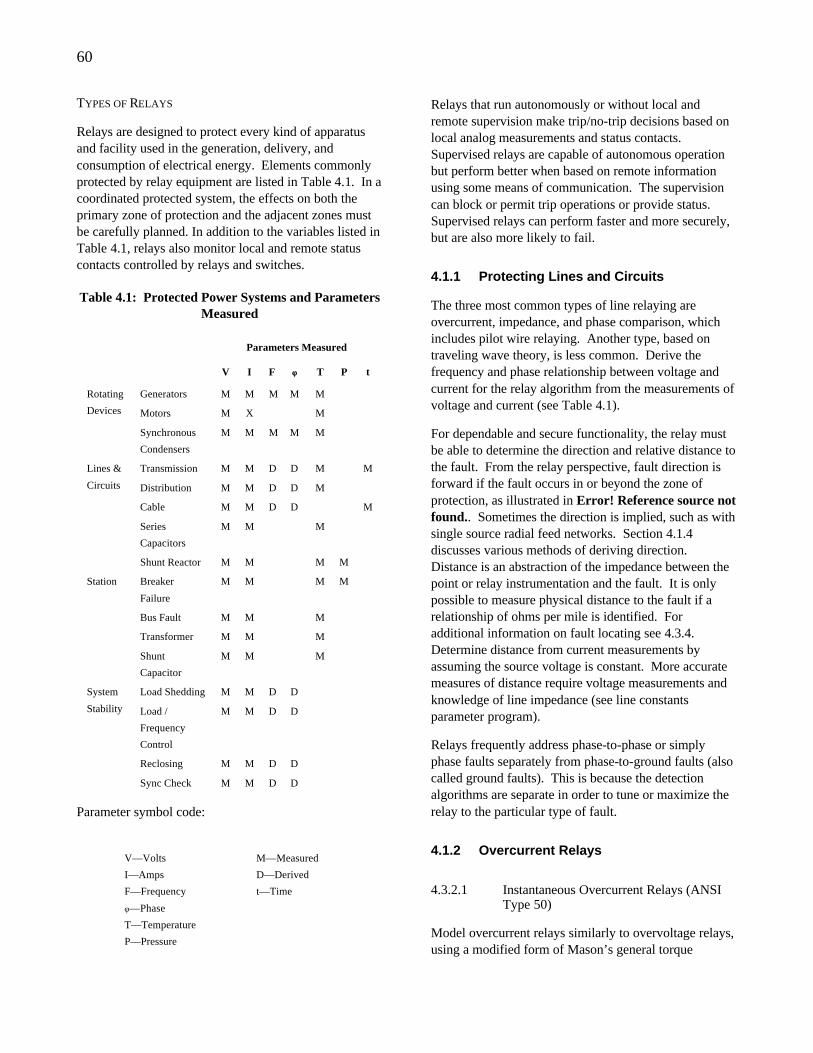
60
TYPES OF RELAYS
Relays are designed to protect every kind of apparatus and facility used in the generation, delivery, and consumption of electrical energy. Elements commonly protected by relay equipment are listed in Table 4.1. In a coordinated protected system, the effects on both the primary zone of protection and the adjacent zones must be carefully planned. In addition to the variables listed in Table 4.1, relays also monitor local and remote status contacts controlled by relays and switches.
Table 4.1: Protected Power Systems and Parameters Measured
Parameters Measured
V I F φφ T P t
Generators M M M M M
Motors M X M
Rotating
Devices
Synchronous
Condensers
M M M M M
Transmission M M D D M M
Distribution M M D D M
Cable M M D D M
Series
Capacitors
M M M
Lines &
Circuits
Shunt Reactor M M M M
Breaker
Failure
M M M M
Bus Fault M M M
Transformer M M M
Station
Shunt
Capacitor
M M M
Load Shedding M M D D
Load /
Frequency
Control
M M D D
Reclosing M M D D
System
Stability
Sync Check M M D D
Parameter symbol code:
V—Volts M—Measured
I—Amps D—Derived
F—Frequency t—Time
φ—Phase
T—Temperature
P—Pressure
Relays that run autonomously or without local and remote supervision make trip/no-trip decisions based on local analog measurements and status contacts. Supervised relays are capable of autonomous operation but perform better when based on remote information using some means of communication. The supervision can block or permit trip operations or provide status. Supervised relays can perform faster and more securely, but are also more likely to fail.
4.1.1 Protecting Lines and Circuits
The three most common types of line relaying are overcurrent, impedance, and phase comparison, which includes pilot wire relaying. Another type, based on traveling wave theory, is less common. Derive the frequency and phase relationship between voltage and current for the relay algorithm from the measurements of voltage and current (see Table 4.1).
For dependable and secure functionality, the relay must be able to determine the direction and relative distance to the fault. From the relay perspective, fault direction is forward if the fault occurs in or beyond the zone of protection, as illustrated in Error! Reference source not found.. Sometimes the direction is implied, such as with single source radial feed networks. Section 4.1.4 discusses various methods of deriving direction. Distance is an abstraction of the impedance between the point or relay instrumentation and the fault. It is only possible to measure physical distance to the fault if a relationship of ohms per mile is identified. For additional information on fault locating see 4.3.4. Determine distance from current measurements by assuming the source voltage is constant. More accurate measures of distance require voltage measurements and knowledge of line impedance (see line constants parameter program).
Relays frequently address phase-to-phase or simply phase faults separately from phase-to-ground faults (also called ground faults). This is because the detection algorithms are separate in order to tune or maximize the relay to the particular type of fault.
4.1.2 Overcurrent Relays
4.3.2.1 Instantaneous Overcurrent Relays (ANSI Type 50)
Model overcurrent relays similarly to overvoltage relays, using a modified form of Mason’s general torque

61
equation as described by (4.2). The relay requires positive torque to operate. Negative K4 provides constant restraining. Solving to the balance point (zero torque) determines the trip current, also commonly called pickup current, as shown in (4.3).
42
1 KIKT −= (4.2)
1
4
K
KI PU = , a constant (4.3)
The induction disk electromechanical relay produces torque in a moveable disk similar to the disk in a residential electrical meter. Consider the case when two time-varying fluxes of the same frequency but different phase, θ, as expressed in (4. 4) and (4. 5) are imposed on a disk as shown in Figure 4.2.
)sin(11 tM ωφ Φ= (4. 4)
)sin(22 θωφ +Φ= tM (4. 5)
At the instant when both fluxes are directed downward and are increasing in magnitude, each flux induces voltage around itself in the rotor, and currents flow in the rotor under the influence of the two voltages. The current produced by one flux reacts with the other flux, and vice versa, to produce forces that act on the disk. Assuming that the disk currents produce insignificant self-inductance, currents iφ1 and iφ2 are in phase with their voltages, resulting in (4. 6 )and (4.7). This produces two mechanical forces opposite in direction so the net force is the difference shown in (4.8).
)cos(11
1 tdt
di M ω
φφ Φ∝∝ (4. 6)
)cos(22
2 θωφ
φ +Φ∝∝ tdt
di M (4.7)
( )21 1212 φφ φφ iiFFF ⋅−⋅∝−= (4.8)
Substituting the quantities of (4. 4) through (4.7) into (4.8) results in the net force. The result is (4. 9), which reduces down to (4.10), which shows the force is proportional to the magnitude of the product of the two fluxes and the phase difference between them.
[ ])sin()cos()cos()sin(21 ttttF MM ωθωωθω +−+ΦΦ∝ (4. 9)
)sin(21 θMMF ΦΦ∝ (4.10)
Figure 4.3 shows the basis of both the residential electric meter and the induction disk relay. The pole shading
forces a phase shift in the flux, θ, that produces the force in (4.10). Since torque is a force times a distance and since the applied current produces identical flux for Φ1 and Φ2, (4.10) can be expressed as (4.1) where K1 accounts for all the proportionality.
ιι φ 1 φ 1
ιι φ 2 φ 2
ιι φ 1 φ 1F2
φ 2φ 2
ιι φ 2 φ 2
F1
φ 1φ 1
Disk
Figure 4.2: Induced Currents and Forces Resulting From Two Flux Paths on a Metallic Disk
To complete the comparison of the induction disk relay to the residential electric meter, meter the power assuming a constant voltage and no restraining spring. This makes K4 zero in (4.2). The meter is free to rotate at a speed proportional to the square of the load current. A counter simply measures the number of disk rotations and applies a kWh conversion per disk revolution.
ShadingRing
ShadingRing
Act
uatin
gS
ourc
e
RotorDirectionof force
Figure 4.3: Shaded-Pole Induction Disk
4.3.2.2 Time-Overcurrent Relays (ANSI Type 51)
The overcurrent relay more or less approximates the operation of the thermal fuse. This similarity is a design characteristic of time-overcurrent relays to accommodate systems that integrate fuse protection with electromechanical, electronic, and microprocessor-based
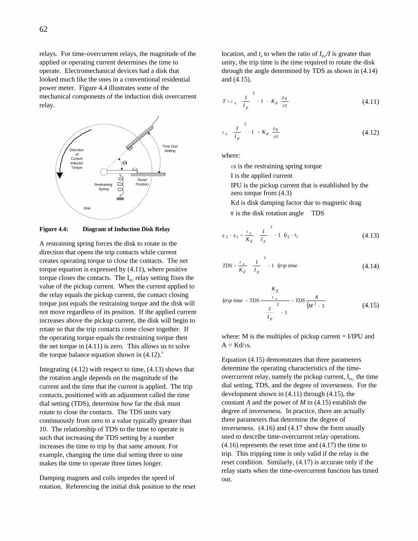
62
relays. For time-overcurrent relays, the magnitude of the applied or operating current determines the time to operate. Electromechanical devices had a disk that looked much like the ones in a conventional residential power meter. Figure 4.4 illustrates some of the mechanical components of the induction disk overcurrent relay.
ResetPosition
Time DialSettingDirection
ofCurrentInducedTorque
Θ
RestrainingSpring
Disk
Figure 4.4: Diagram of Induction Disk Relay
A restraining spring forces the disk to rotate in the direction that opens the trip contacts while current creates operating torque to close the contacts. The net torque equation is expressed by (4.11), where positive torque closes the contacts. The IPU relay setting fixes the value of the pickup current. When the current applied to the relay equals the pickup current, the contact closing torque just equals the restraining torque and the disk will not move regardless of its position. If the applied current increases above the pickup current, the disk will begin to rotate so that the trip contacts come closer together. If the operating torque equals the restraining torque then the net torque in (4.11) is zero. This allows us to solve the torque balance equation shown in (4.12).ii
Integrating (4.12) with respect to time, (4.13) shows that the rotation angle depends on the magnitude of the current and the time that the current is applied. The trip contacts, positioned with an adjustment called the time dial setting (TDS), determine how far the disk must rotate to close the contacts. The TDS units vary continuously from zero to a value typically greater than 10. The relationship of TDS to the time to operate is such that increasing the TDS setting by a number increases the time to trip by that same amount. For example, changing the time dial setting three to nine makes the time to operate three times longer.
Damping magnets and coils impedes the speed of rotation. Referencing the initial disk position to the reset
location, and t0 to when the ratio of IPU/I is greater than unity, the trip time is the time required to rotate the disk through the angle determined by TDS as shown in (4.14) and (4.15).
∂
∂−
−
=
tK
I
IT d
ps
θτ 1
2
(4.11)
∂
∂=
−
tK
I
Id
ps
θτ 1
2
(4.12)
where:
τs is the restraining spring torque I is the applied current
IPU is the pickup current that is established by the zero torque from (4.3)
Kd is disk damping factor due to magnetic drag
θ is the disk rotation angle ∝ TDS
( )12
2
12 1 ttI
I
K pd
s −
−
=−
τθθ (4.13)
( )timetripI
I
KTDS
pd
s
−
= 1
2τ (4.14)
( ) ( )11
22 −=
−
=M
ATDS
I
I
K
TDStimetrip
p
s
d
τ (4.15)
where: M is the multiples of pickup current = I/IPU and A = Kd/τs.
Equation (4.15) demonstrates that three parameters determine the operating characteristics of the time-overcurrent relay, namely the pickup current, IPU, the time dial setting, TDS, and the degree of inverseness. For the development shown in (4.11) through (4.15), the constant A and the power of M in (4.15) establish the degree of inverseness. In practice, there are actually three parameters that determine the degree of inverseness. (4.16) and (4.17 show the form usually used to describe time-overcurrent relay operations. (4.16) represents the reset time and (4.17) the time to trip. This tripping time is only valid if the relay is the reset condition. Similarly, (4.17) is accurate only if the relay starts when the time-overcurrent function has timed out.
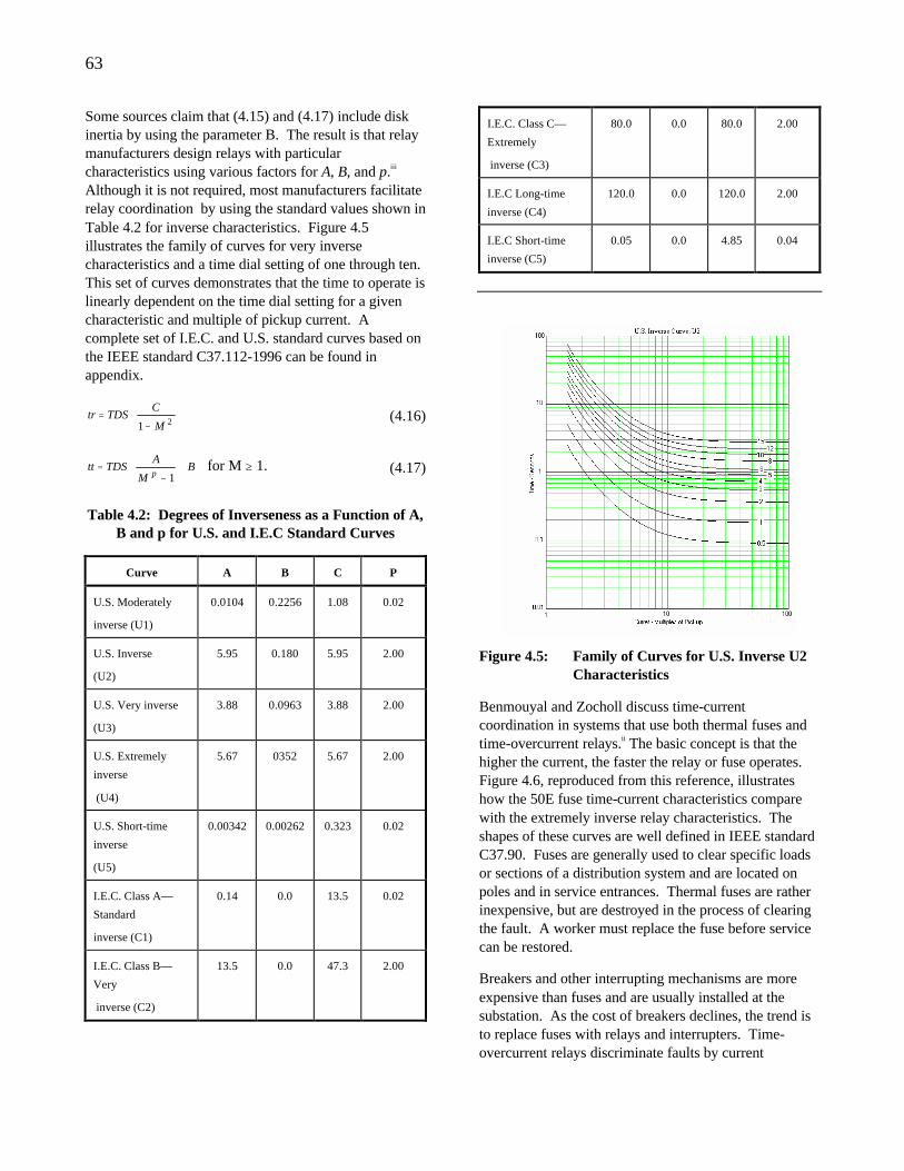
63
Some sources claim that (4.15) and (4.17) include disk inertia by using the parameter B. The result is that relay manufacturers design relays with particular characteristics using various factors for A, B, and p.iii Although it is not required, most manufacturers facilitate relay coordination by using the standard values shown in Table 4.2 for inverse characteristics. Figure 4.5 illustrates the family of curves for very inverse characteristics and a time dial setting of one through ten. This set of curves demonstrates that the time to operate is linearly dependent on the time dial setting for a given characteristic and multiple of pickup current. A complete set of I.E.C. and U.S. standard curves based on the IEEE standard C37.112-1996 can be found in appendix.
−=
21 M
CTDStr (4.16)
+
−= B
M
ATDStt
p 1 for M ≥ 1. (4.17)
Table 4.2: Degrees of Inverseness as a Function of A, B and p for U.S. and I.E.C Standard Curves
Curve A B C P
U.S. Moderately
inverse (U1)
0.0104 0.2256 1.08 0.02
U.S. Inverse
(U2)
5.95 0.180 5.95 2.00
U.S. Very inverse
(U3)
3.88 0.0963 3.88 2.00
U.S. Extremely
inverse
(U4)
5.67 0352 5.67 2.00
U.S. Short-time
inverse
(U5)
0.00342 0.00262 0.323 0.02
I.E.C. Class A—
Standard
inverse (C1)
0.14 0.0 13.5 0.02
I.E.C. Class B—
Very
inverse (C2)
13.5 0.0 47.3 2.00
I.E.C. Class C—
Extremely
inverse (C3)
80.0 0.0 80.0 2.00
I.E.C Long-time
inverse (C4)
120.0 0.0 120.0 2.00
I.E.C Short-time
inverse (C5)
0.05 0.0 4.85 0.04
Figure 4.5: Family of Curves for U.S. Inverse U2 Characteristics
Benmouyal and Zocholl discuss time-current coordination in systems that use both thermal fuses and time-overcurrent relays.ii The basic concept is that the higher the current, the faster the relay or fuse operates. Figure 4.6, reproduced from this reference, illustrates how the 50E fuse time-current characteristics compare with the extremely inverse relay characteristics. The shapes of these curves are well defined in IEEE standard C37.90. Fuses are generally used to clear specific loads or sections of a distribution system and are located on poles and in service entrances. Thermal fuses are rather inexpensive, but are destroyed in the process of clearing the fault. A worker must replace the fuse before service can be restored.
Breakers and other interrupting mechanisms are more expensive than fuses and are usually installed at the substation. As the cost of breakers declines, the trend is to replace fuses with relays and interrupters. Time-overcurrent relays discriminate faults by current
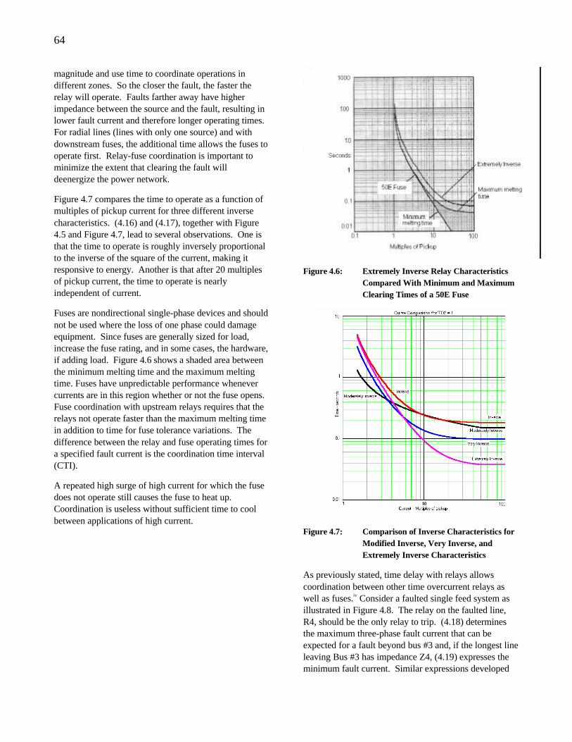
64
magnitude and use time to coordinate operations in different zones. So the closer the fault, the faster the relay will operate. Faults farther away have higher impedance between the source and the fault, resulting in lower fault current and therefore longer operating times. For radial lines (lines with only one source) and with downstream fuses, the additional time allows the fuses to operate first. Relay-fuse coordination is important to minimize the extent that clearing the fault will deenergize the power network.
Figure 4.7 compares the time to operate as a function of multiples of pickup current for three different inverse characteristics. (4.16) and (4.17), together with Figure 4.5 and Figure 4.7, lead to several observations. One is that the time to operate is roughly inversely proportional to the inverse of the square of the current, making it responsive to energy. Another is that after 20 multiples of pickup current, the time to operate is nearly independent of current.
Fuses are nondirectional single-phase devices and should not be used where the loss of one phase could damage equipment. Since fuses are generally sized for load, increase the fuse rating, and in some cases, the hardware, if adding load. Figure 4.6 shows a shaded area between the minimum melting time and the maximum melting time. Fuses have unpredictable performance whenever currents are in this region whether or not the fuse opens. Fuse coordination with upstream relays requires that the relays not operate faster than the maximum melting time in addition to time for fuse tolerance variations. The difference between the relay and fuse operating times for a specified fault current is the coordination time interval (CTI).
A repeated high surge of high current for which the fuse does not operate still causes the fuse to heat up. Coordination is useless without sufficient time to cool between applications of high current.
Figure 4.6: Extremely Inverse Relay Characteristics Compared With Minimum and Maximum Clearing Times of a 50E Fuse
Figure 4.7: Comparison of Inverse Characteristics for Modified Inverse, Very Inverse, and Extremely Inverse Characteristics
As previously stated, time delay with relays allows coordination between other time overcurrent relays as well as fuses.iv Consider a faulted single feed system as illustrated in Figure 4.8. The relay on the faulted line, R4, should be the only relay to trip. (4.18) determines the maximum three-phase fault current that can be expected for a fault beyond bus #3 and, if the longest line leaving Bus #3 has impedance Z4, (4.19) expresses the minimum fault current. Similar expressions developed
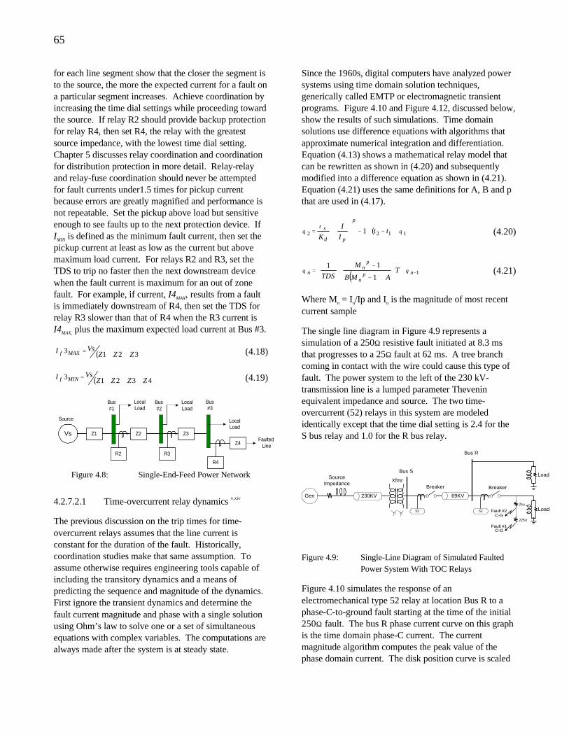
65
for each line segment show that the closer the segment is to the source, the more the expected current for a fault on a particular segment increases. Achieve coordination by increasing the time dial settings while proceeding toward the source. If relay R2 should provide backup protection for relay R4, then set R4, the relay with the greatest source impedance, with the lowest time dial setting. Chapter 5 discusses relay coordination and coordination for distribution protection in more detail. Relay-relay and relay-fuse coordination should never be attempted for fault currents under1.5 times for pickup current because errors are greatly magnified and performance is not repeatable. Set the pickup above load but sensitive enough to see faults up to the next protection device. If IMIN is defined as the minimum fault current, then set the pickup current at least as low as the current but above maximum load current. For relays R2 and R3, set the TDS to trip no faster then the next downstream device when the fault current is maximum for an out of zone fault. For example, if current, I4MAX, results from a fault is immediately downstream of R4, then set the TDS for relay R3 slower than that of R4 when the R3 current is I4MAX, plus the maximum expected load current at Bus #3.
( )3213 ZZZVsI MAXf ++
= (4.18)
( )43213 ZZZZVsI MINf +++
= (4.19)
Vs Z1
LocalLoad
LocalLoad
LocalLoad
FaultedLine
Bus#1
Bus#2
Bus#3
Z3
Z4
Z2
Source
R3R2
R4
Figure 4.8: Single-End-Feed Power Network
4.2.7.2.1 Time-overcurrent relay dynamics v,xiv
The previous discussion on the trip times for time-overcurrent relays assumes that the line current is constant for the duration of the fault. Historically, coordination studies make that same assumption. To assume otherwise requires engineering tools capable of including the transitory dynamics and a means of predicting the sequence and magnitude of the dynamics. First ignore the transient dynamics and determine the fault current magnitude and phase with a single solution using Ohm’s law to solve one or a set of simultaneous equations with complex variables. The computations are always made after the system is at steady state.
Since the 1960s, digital computers have analyzed power systems using time domain solution techniques, generically called EMTP or electromagnetic transient programs. Figure 4.10 and Figure 4.12, discussed below, show the results of such simulations. Time domain solutions use difference equations with algorithms that approximate numerical integration and differentiation. Equation (4.13) shows a mathematical relay model that can be rewritten as shown in (4.20) and subsequently modified into a difference equation as shown in (4.21). Equation (4.21) uses the same definitions for A, B and p that are used in (4.17).
( ) 1122 1 θτ
θ +−
−
= tt
I
I
K
p
pd
s (4.20)
( ) 11
11−+
+−
−
= np
n
pn
n TAMB
M
TDSθθ (4.21)
Where Mn = In/Ip and In is the magnitude of most recent current sample
The single line diagram in Figure 4.9 represents a simulation of a 250Ω resistive fault initiated at 8.3 ms that progresses to a 25Ω fault at 62 ms. A tree branch coming in contact with the wire could cause this type of fault. The power system to the left of the 230 kV-transmission line is a lumped parameter Thevenin equivalent impedance and source. The two time-overcurrent (52) relays in this system are modeled identically except that the time dial setting is 2.4 for the S bus relay and 1.0 for the R bus relay.
Gen
XfmrBreaker Breaker
SourceImpedance
230KV
Fault #2C-G
Fault #1C-G
69KV
52 52
Bus S
Bus R
Load
Load
225Ω
25Ω
Figure 4.9: Single-Line Diagram of Simulated Faulted Power System With TOC Relays
Figure 4.10 simulates the response of an electromechanical type 52 relay at location Bus R to a phase-C-to-ground fault starting at the time of the initial 250Ω fault. The bus R phase current curve on this graph is the time domain phase-C current. The current magnitude algorithm computes the peak value of the phase domain current. The disk position curve is scaled
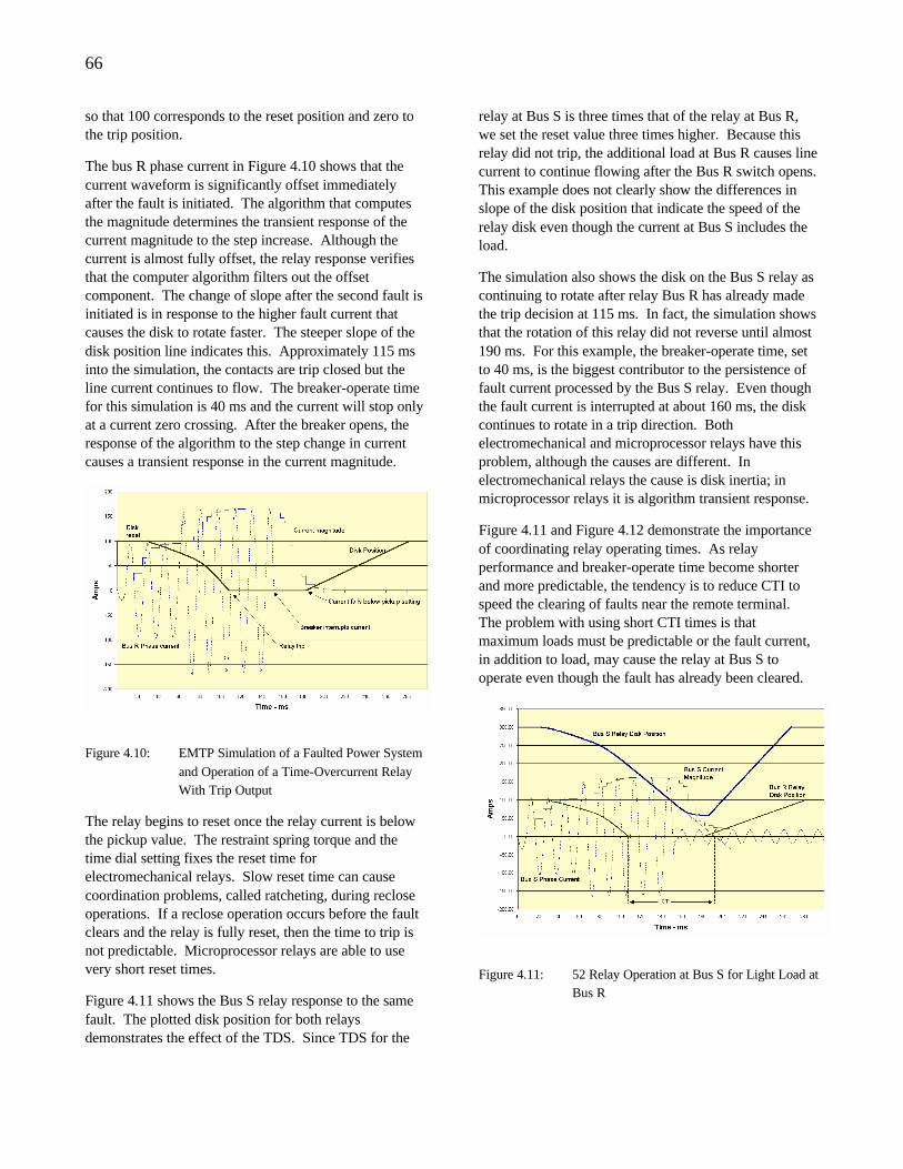
66
so that 100 corresponds to the reset position and zero to the trip position.
The bus R phase current in Figure 4.10 shows that the current waveform is significantly offset immediately after the fault is initiated. The algorithm that computes the magnitude determines the transient response of the current magnitude to the step increase. Although the current is almost fully offset, the relay response verifies that the computer algorithm filters out the offset component. The change of slope after the second fault is initiated is in response to the higher fault current that causes the disk to rotate faster. The steeper slope of the disk position line indicates this. Approximately 115 ms into the simulation, the contacts are trip closed but the line current continues to flow. The breaker-operate time for this simulation is 40 ms and the current will stop only at a current zero crossing. After the breaker opens, the response of the algorithm to the step change in current causes a transient response in the current magnitude.
Figure 4.10: EMTP Simulation of a Faulted Power System and Operation of a Time-Overcurrent Relay With Trip Output
The relay begins to reset once the relay current is below the pickup value. The restraint spring torque and the time dial setting fixes the reset time for electromechanical relays. Slow reset time can cause coordination problems, called ratcheting, during reclose operations. If a reclose operation occurs before the fault clears and the relay is fully reset, then the time to trip is not predictable. Microprocessor relays are able to use very short reset times.
Figure 4.11 shows the Bus S relay response to the same fault. The plotted disk position for both relays demonstrates the effect of the TDS. Since TDS for the
relay at Bus S is three times that of the relay at Bus R, we set the reset value three times higher. Because this relay did not trip, the additional load at Bus R causes line current to continue flowing after the Bus R switch opens. This example does not clearly show the differences in slope of the disk position that indicate the speed of the relay disk even though the current at Bus S includes the load.
The simulation also shows the disk on the Bus S relay as continuing to rotate after relay Bus R has already made the trip decision at 115 ms. In fact, the simulation shows that the rotation of this relay did not reverse until almost 190 ms. For this example, the breaker-operate time, set to 40 ms, is the biggest contributor to the persistence of fault current processed by the Bus S relay. Even though the fault current is interrupted at about 160 ms, the disk continues to rotate in a trip direction. Both electromechanical and microprocessor relays have this problem, although the causes are different. In electromechanical relays the cause is disk inertia; in microprocessor relays it is algorithm transient response.
Figure 4.11 and Figure 4.12 demonstrate the importance of coordinating relay operating times. As relay performance and breaker-operate time become shorter and more predictable, the tendency is to reduce CTI to speed the clearing of faults near the remote terminal. The problem with using short CTI times is that maximum loads must be predictable or the fault current, in addition to load, may cause the relay at Bus S to operate even though the fault has already been cleared.
Figure 4.11: 52 Relay Operation at Bus S for Light Load at Bus R
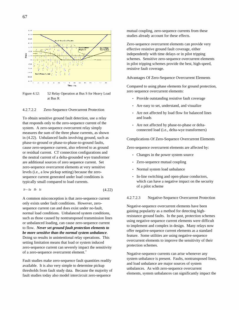
67
Figure 4.12: 52 Relay Operation at Bus S for Heavy Load at Bus R
4.2.7.2.2 Zero-Sequence Overcurrent Protection
To obtain sensitive ground fault detection, use a relay that responds only to the zero-sequence current of the system. A zero-sequence overcurrent relay simply measures the sum of the three phase currents, as shown in (4.22). Unbalanced faults involving ground, such as phase-to-ground or phase-to-phase-to-ground faults, cause zero-sequence current, also referred to as ground or residual current. CT connection configurations and the neutral current of a delta-grounded wye transformer are additional sources of zero sequence current. Set zero-sequence overcurrent elements at very sensitive levels (i.e., a low pickup setting) because the zero-sequence current generated under load conditions is typically small compared to load currents.
IcIbIaIr ++= (4.22)
A common misconception is that zero-sequence current only exists under fault conditions. However, zero-sequence current can and does exist under no-fault, normal load conditions. Unbalanced system conditions, such as those caused by nontransposed transmission lines or unbalanced loading, can cause zero-sequence current to flow. Never set ground fault protection elements to be more sensitive than the normal system unbalance. Doing so results in unintentional relay operations. This setting limitation means that load or system induced zero-sequence current can severely impact the sensitivity of a zero-sequence overcurrent element.vi
Fault studies make zero-sequence fault quantities readily available. It is also very simple to determine pickup thresholds from fault study data. Because the majority of fault studies today also model intercircuit zero-sequence
mutual coupling, zero-sequence currents from these studies already account for these effects.
Zero-sequence overcurrent elements can provide very effective resistive ground fault coverage, either independently with time delays or in pilot tripping schemes. Sensitive zero-sequence overcurrent elements in pilot tripping schemes provide the best, high-speed, resistive fault coverage.
Advantages Of Zero-Sequence Overcurrent Elements
Compared to using phase elements for ground protection, zero sequence overcurrent elements:
• Provide outstanding resistive fault coverage
• Are easy to set, understand, and visualize
• Are not affected by load flow for balanced lines and loads
• Are not affected by phase-to-phase or delta-connected load (i.e., delta-wye transformers)
Complications Of Zero-Sequence Overcurrent Elements
Zero-sequence overcurrent elements are affected by:
• Changes in the power system source
• Zero-sequence mutual coupling
• Normal system load unbalance
• In-line switching and open-phase conductors, which can have a negative impact on the security of a pilot scheme
4.2.7.2.3 Negative-Sequence Overcurrent Protection
Negative-sequence overcurrent elements have been gaining popularity as a method for detecting high-resistance ground faults. In the past, protection schemes using negative-sequence current elements were difficult to implement and complex in design. Many relays now offer negative-sequence current elements as a standard feature. Some utilities are using negative-sequence overcurrent elements to improve the sensitivity of their protection schemes.
Negative-sequence currents can arise whenever any system unbalance is present. Faults, nontransposed lines, and load unbalance are major sources of system unbalances. As with zero-sequence overcurrent elements, system unbalances can significantly impact the
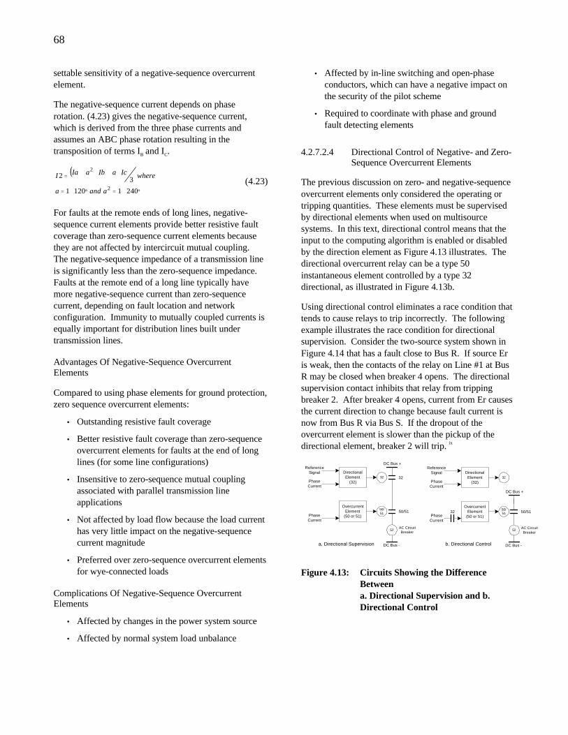
68
settable sensitivity of a negative-sequence overcurrent element.
The negative-sequence current depends on phase rotation. (4.23) gives the negative-sequence current, which is derived from the three phase currents and assumes an ABC phase rotation resulting in the transposition of terms IB and IC.
( )
°∠=°∠=
⋅+⋅+=
24011201
32
2
2
aanda
whereIcaIbaIaI (4.23)
For faults at the remote ends of long lines, negative-sequence current elements provide better resistive fault coverage than zero-sequence current elements because they are not affected by intercircuit mutual coupling. The negative-sequence impedance of a transmission line is significantly less than the zero-sequence impedance. Faults at the remote end of a long line typically have more negative-sequence current than zero-sequence current, depending on fault location and network configuration. Immunity to mutually coupled currents is equally important for distribution lines built under transmission lines.
Advantages Of Negative-Sequence Overcurrent Elements
Compared to using phase elements for ground protection, zero sequence overcurrent elements:
• Outstanding resistive fault coverage
• Better resistive fault coverage than zero-sequence overcurrent elements for faults at the end of long lines (for some line configurations)
• Insensitive to zero-sequence mutual coupling associated with parallel transmission line applications
• Not affected by load flow because the load current has very little impact on the negative-sequence current magnitude
• Preferred over zero-sequence overcurrent elements for wye-connected loads
Complications Of Negative-Sequence Overcurrent Elements
• Affected by changes in the power system source
• Affected by normal system load unbalance
• Affected by in-line switching and open-phase conductors, which can have a negative impact on the security of the pilot scheme
• Required to coordinate with phase and ground fault detecting elements
4.2.7.2.4 Directional Control of Negative- and Zero-Sequence Overcurrent Elements
The previous discussion on zero- and negative-sequence overcurrent elements only considered the operating or tripping quantities. These elements must be supervised by directional elements when used on multisource systems. In this text, directional control means that the input to the computing algorithm is enabled or disabled by the direction element as Figure 4.13 illustrates. The directional overcurrent relay can be a type 50 instantaneous element controlled by a type 32 directional, as illustrated in Figure 4.13b.
Using directional control eliminates a race condition that tends to cause relays to trip incorrectly. The following example illustrates the race condition for directional supervision. Consider the two-source system shown in Figure 4.14 that has a fault close to Bus R. If source Er is weak, then the contacts of the relay on Line #1 at Bus R may be closed when breaker 4 opens. The directional supervision contact inhibits that relay from tripping breaker 2. After breaker 4 opens, current from Er causes the current direction to change because fault current is now from Bus R via Bus S. If the dropout of the overcurrent element is slower than the pickup of the directional element, breaker 2 will trip. ix
32DirectionalElement
(32)
ReferenceSignal
PhaseCurrent
50/51
OvercurrentElement
(50 or 51)PhaseCurrent
50/51
52
DC Bus -
AC CircuitBreaker
b. Directional Control
32
DC Bus +
32DirectionalElement
(32)
ReferenceSignal
PhaseCurrent
50/51
OvercurrentElement
(50 or 51)PhaseCurrent
32
50/51
52
DC Bus +
DC Bus -
AC CircuitBreaker
a. Directional Supervision
Figure 4.13: Circuits Showing the Difference Between a. Directional Supervision and b. Directional Control
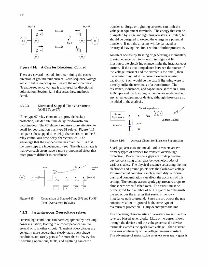
69
R
R
R
R
Bus S
Es
Line #2
Line #1
3
1
4
2
Bus R
FaultEr
Figure 4.14: A Case for Directional Control
There are several methods for determining the correct direction of ground fault current. Zero-sequence voltage and current reference quantities are the most common. Negative-sequence voltage is also used for directional polarization. Section 4.1.4 discusses these methods in detail.
4.3.2.3 Directional Stepped-Time Overcurrent (ANSI Type 67)
If the type 67 relay element is to provide backup protection, use definite time delay for downstream coordination. The 67 element requires more attention to detail for coordination than type 51 relays. Figure 4.15 compares the stepped-time delay characteristics to the 51 relay continuous time delay characteristics. The advantage that the stepped-time has over the 51 is that the time steps are independently set. The disadvantage is that overreach errors have a more pronounced effect that often proves difficult to coordinate.
Bus S
2G 1
Load1
Load2
Load3
Load4
F1 F2 F3 F4
Load 5
Increasingtime
51
67
Figure 4.15: Comparison of Stepped-Time (67) and I2t (51) Time-Overcurrent Relaying
4.1.3 Instantaneous Overvoltage relays
Overvoltage conditions can harm equipment by breaking down insulation, leading to a low-impedance fault to ground or to another circuit. Transient overvoltages are generally more severe than steady-state overvoltage conditions and rarely persist for more than a few cycles. Switching operations, faults, and lightning can cause
transients. Surge or lightning arresters can limit the voltage at equipment terminals. The energy that can be dissipated by surge and lightning arresters is limited, but should be designed to exceed the energy in a potential transient. If not, the arresters will be damaged or destroyed leaving the circuit without further protection.
Arresters operate by flashing or generating a momentary low-impedance path to ground. As Figure 4.16 illustrates, the circuit inductance limits the instantaneous current. If the circuit impedance between the source of the voltage transient and the arrester is too small, then the arrester may fail if the current exceeds arrester capability. Such would be the case if lightning were to directly strike the terminals of a transformer. The resistance, inductance, and capacitance shown in Figure 4.16 represent the line, bus, or conductor model and not any actual equipment or device, although those can also be added to the analysis.
PowerEquipment
Arrester
Circuit Impedance
Voltage Source
Figure 4.16: Arrester Circuit for Transient Suppression
Spark gap arresters and metal oxide arresters are two primary types of devices for transient overvoltage protection. Protective spark gaps are crude protection devices consisting of air gaps between electrodes of various shapes. The physical distance separating the line electrodes and ground points sets the flash-over voltage. Environmental conditions such as humidity, airborne dust, and contamination can affect the accuracy of this setting. The voltage across spark gap arresters drops to almost zero when flashed over. The circuit must be deenergized for a number of 60 Hz cycles to extinguish the arc across the arrester that sustains the low-impedance path to ground. Since the arc across the gap constitutes a line-to-ground fault, some type of overcurrent protection usually deenergizes the line.
The operating characteristics of arresters are similar to a reversed biased zener diode. Little or no current flows through the device until the voltage across the device terminals exceeds the spark over voltage. Then current increases nonlinearly while voltage remains constant. The advantage of metal oxide arresters over spark gaps is
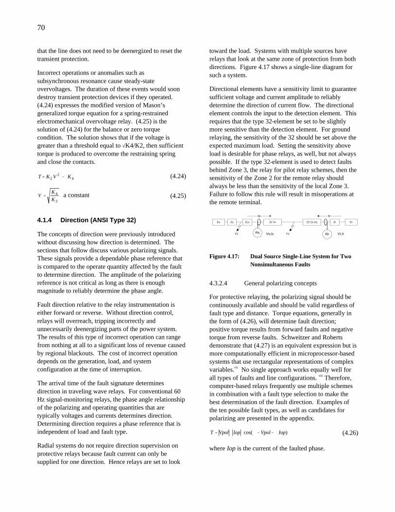
70
that the line does not need to be deenergized to reset the transient protection.
Incorrect operations or anomalies such as subsynchronous resonance cause steady-state overvoltages. The duration of these events would soon destroy transient protection devices if they operated. (4.24) expresses the modified version of Mason’s generalized torque equation for a spring-restrained electromechanical overvoltage relay. (4.25) is the solution of (4.24) for the balance or zero torque condition. The solution shows that if the voltage is greater than a threshold equal to √K4/K2, then sufficient torque is produced to overcome the restraining spring and close the contacts.
42
2 KVKT −= (4.24)
2
4
K
KV = a constant (4.25)
4.1.4 Direction (ANSI Type 32)
The concepts of direction were previously introduced without discussing how direction is determined. The sections that follow discuss various polarizing signals. These signals provide a dependable phase reference that is compared to the operate quantity affected by the fault to determine direction. The amplitude of the polarizing reference is not critical as long as there is enough magnitude to reliably determine the phase angle.
Fault direction relative to the relay instrumentation is either forward or reverse. Without direction control, relays will overreach, tripping incorrectly and unnecessarily deenergizing parts of the power system. The results of this type of incorrect operation can range from nothing at all to a significant loss of revenue caused by regional blackouts. The cost of incorrect operation depends on the generation, load, and system configuration at the time of interruption.
The arrival time of the fault signature determines direction in traveling wave relays. For conventional 60 Hz signal-monitoring relays, the phase angle relationship of the polarizing and operating quantities that are typically voltages and currents determines direction. Determining direction requires a phase reference that is independent of load and fault type.
Radial systems do not require direction supervision on protective relays because fault current can only be supplied for one direction. Hence relays are set to look
toward the load. Systems with multiple sources have relays that look at the same zone of protection from both directions. Figure 4.17 shows a single-line diagram for such a system.
Directional elements have a sensitivity limit to guarantee sufficient voltage and current amplitude to reliably determine the direction of current flow. The directional element controls the input to the detection element. This requires that the type 32-element be set to be slightly more sensitive than the detection element. For ground relaying, the sensitivity of the 32 should be set above the expected maximum load. Setting the sensitivity above load is desirable for phase relays, as well, but not always possible. If the type 32-element is used to detect faults behind Zone 3, the relay for pilot relay schemes, then the sensitivity of the Zone 2 for the remote relay should always be less than the sensitivity of the local Zone 3. Failure to follow this rule will result in misoperations at the remote terminal.
Es Zs ZL*m ZL*(1-m) ErZr
Rs RrVs,Is Vr,Ir
Is Ir
ZLs
F2 F1
Figure 4.17: Dual Source Single-Line System for Two Nonsimultaneous Faults
4.3.2.4 General polarizing concepts
For protective relaying, the polarizing signal should be continuously available and should be valid regardless of fault type and distance. Torque equations, generally in the form of (4.26), will determine fault direction; positive torque results from forward faults and negative torque from reverse faults. Schweitzer and Roberts demonstrate that (4.27) is an equivalent expression but is more computationally efficient in microprocessor-based systems that use rectangular representations of complex variables.vii No single approach works equally well for all types of faults and line configurations. viii Therefore, computer-based relays frequently use multiple schemes in combination with a fault type selection to make the best determination of the fault direction. Examples of the ten possible fault types, as well as candidates for polarizing are presented in the appendix.
)cos( IopVpolIopVpolT ∠−−∠⋅⋅= (4.26)
where Iop is the current of the faulted phase.
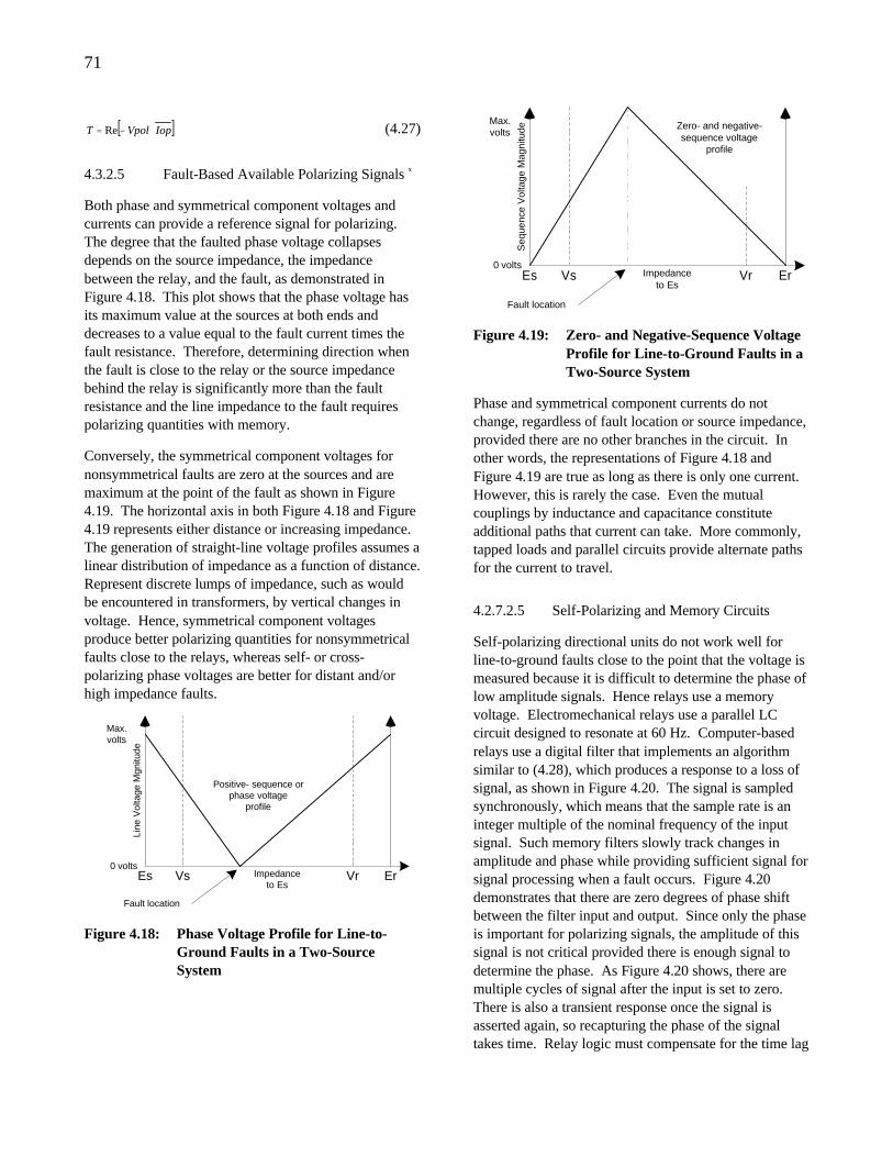
71
[ ]IopVpolT ⋅−= Re (4.27)
4.3.2.5 Fault-Based Available Polarizing Signals x
Both phase and symmetrical component voltages and currents can provide a reference signal for polarizing. The degree that the faulted phase voltage collapses depends on the source impedance, the impedance between the relay, and the fault, as demonstrated in Figure 4.18. This plot shows that the phase voltage has its maximum value at the sources at both ends and decreases to a value equal to the fault current times the fault resistance. Therefore, determining direction when the fault is close to the relay or the source impedance behind the relay is significantly more than the fault resistance and the line impedance to the fault requires polarizing quantities with memory.
Conversely, the symmetrical component voltages for nonsymmetrical faults are zero at the sources and are maximum at the point of the fault as shown in Figure 4.19. The horizontal axis in both Figure 4.18 and Figure 4.19 represents either distance or increasing impedance. The generation of straight-line voltage profiles assumes a linear distribution of impedance as a function of distance. Represent discrete lumps of impedance, such as would be encountered in transformers, by vertical changes in voltage. Hence, symmetrical component voltages produce better polarizing quantities for nonsymmetrical faults close to the relays, whereas self- or cross-polarizing phase voltages are better for distant and/or high impedance faults.
Line
Vol
tage
Mgn
itude
Impedanceto Es
Es Vs ErVr0 volts
Positive- sequence orphase voltage
profile
Fault location
Max.volts
Figure 4.18: Phase Voltage Profile for Line-to-Ground Faults in a Two-Source System
Seq
uenc
e V
olta
ge M
agni
tude
Impedanceto Es
Es Vs ErVr0 volts
Zero- and negative-sequence voltage
profile
Fault location
Max.volts
Figure 4.19: Zero- and Negative-Sequence Voltage Profile for Line-to-Ground Faults in a Two-Source System
Phase and symmetrical component currents do not change, regardless of fault location or source impedance, provided there are no other branches in the circuit. In other words, the representations of Figure 4.18 and Figure 4.19 are true as long as there is only one current. However, this is rarely the case. Even the mutual couplings by inductance and capacitance constitute additional paths that current can take. More commonly, tapped loads and parallel circuits provide alternate paths for the current to travel.
4.2.7.2.5 Self-Polarizing and Memory Circuits
Self-polarizing directional units do not work well for line-to-ground faults close to the point that the voltage is measured because it is difficult to determine the phase of low amplitude signals. Hence relays use a memory voltage. Electromechanical relays use a parallel LC circuit designed to resonate at 60 Hz. Computer-based relays use a digital filter that implements an algorithm similar to (4.28), which produces a response to a loss of signal, as shown in Figure 4.20. The signal is sampled synchronously, which means that the sample rate is an integer multiple of the nominal frequency of the input signal. Such memory filters slowly track changes in amplitude and phase while providing sufficient signal for signal processing when a fault occurs. Figure 4.20 demonstrates that there are zero degrees of phase shift between the filter input and output. Since only the phase is important for polarizing signals, the amplitude of this signal is not critical provided there is enough signal to determine the phase. As Figure 4.20 shows, there are multiple cycles of signal after the input is set to zero. There is also a transient response once the signal is asserted again, so recapturing the phase of the signal takes time. Relay logic must compensate for the time lag
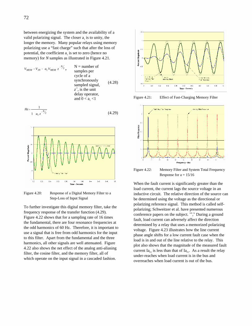
72
between energizing the system and the availability of a valid polarizing signal. The closer a1 is to unity, the longer the memory. Many popular relays using memory polarizing use a “fast charge” such that after the loss of potential, the coefficient a1 is set to zero (hence no memory) for N samples as illustrated in Figure 4.21.
21
N
MEMINMEM zVaVV−
−= , N = number of samples per cycle of a synchronously sampled signal, z-1, is the unit delay operator, and 0 < a1 <1
(4.28)
211
1N
za
Hz−
+
=
(4.29)
Figure 4.20: Response of a Digital Memory Filter to a Step-Loss of Input Signal
To further investigate this digital memory filter, take the frequency response of the transfer function (4.29). Figure 4.22 shows that for a sampling rate of 16 times the fundamental, there are four resonance frequencies at the odd harmonics of 60 Hz. Therefore, it is important to use a signal that is free from odd harmonics for the input to this filter. Apart from the fundamental and the three harmonics, all other signals are well attenuated. Figure 4.22 also shows the net effect of the analog anti-aliasing filter, the cosine filter, and the memory filter, all of which operate on the input signal in a cascaded fashion.
Figure 4.21: Effect of Fast-Charging Memory Filter
Figure 4.22: Memory Filter and System Total Frequency Response for a = 15/16
When the fault current is significantly greater than the load current, the current lags the source voltage in an inductive circuit. The relative direction of the source can be determined using the voltage as the directional or polarizing reference signal. This method is called self-polarizing; Schweitzer et al. have presented numerous conference papers on the subject. viii,ix During a ground fault, load current can adversely affect the direction determined by a relay that uses a memorized polarizing voltage. Figure 4.23 illustrates how the line current phase angle shifts for a low current fault case when the load is in and out of the line relative to the relay. This plot also shows that the magnitude of the measured fault current IaF2 is less than that of IaF1. As a result the relay under-reaches when load current is in the bus and overreaches when load current is out of the bus.
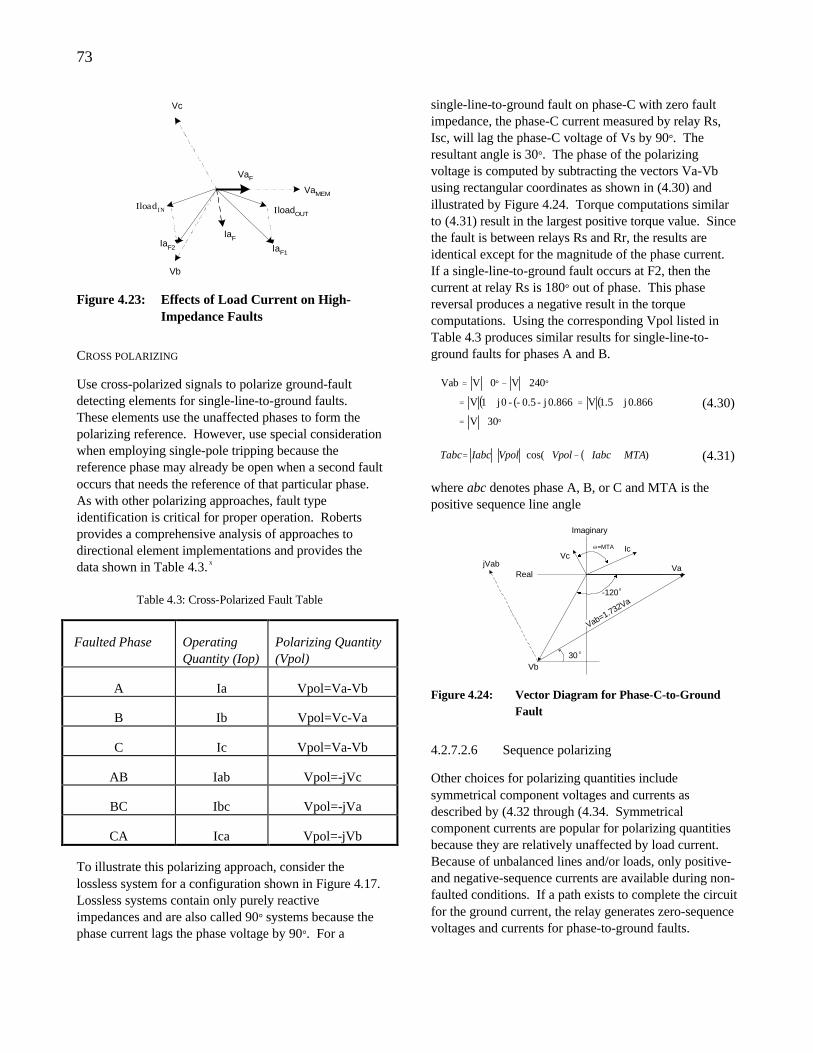
73
Vc
VaMEM
Vb
VaF
IaF
IloadOUTIloadIN
IaF1IaF2
Figure 4.23: Effects of Load Current on High-Impedance Faults
CROSS POLARIZING
Use cross-polarized signals to polarize ground-fault detecting elements for single-line-to-ground faults. These elements use the unaffected phases to form the polarizing reference. However, use special consideration when employing single-pole tripping because the reference phase may already be open when a second fault occurs that needs the reference of that particular phase. As with other polarizing approaches, fault type identification is critical for proper operation. Roberts provides a comprehensive analysis of approaches to directional element implementations and provides the data shown in Table 4.3. x
Table 4.3: Cross-Polarized Fault Table
Faulted Phase Operating Quantity (Iop)
Polarizing Quantity (Vpol)
A Ia Vpol=Va-Vb
B Ib Vpol=Vc-Va
C Ic Vpol=Va-Vb
AB Iab Vpol=-jVc
BC Ibc Vpol=-jVa
CA Ica Vpol=-jVb
To illustrate this polarizing approach, consider the lossless system for a configuration shown in Figure 4.17. Lossless systems contain only purely reactive impedances and are also called 90° systems because the phase current lags the phase voltage by 90°. For a
single-line-to-ground fault on phase-C with zero fault impedance, the phase-C current measured by relay Rs, Isc, will lag the phase-C voltage of Vs by 90°. The resultant angle is 30°. The phase of the polarizing voltage is computed by subtracting the vectors Va-Vb using rectangular coordinates as shown in (4.30) and illustrated by Figure 4.24. Torque computations similar to (4.31) result in the largest positive torque value. Since the fault is between relays Rs and Rr, the results are identical except for the magnitude of the phase current. If a single-line-to-ground fault occurs at F2, then the current at relay Rs is 180° out of phase. This phase reversal produces a negative result in the torque computations. Using the corresponding Vpol listed in Table 4.3 produces similar results for single-line-to-ground faults for phases A and B.
( ) ( )( )°∠=
+=+=
°∠−°∠=
30V
0.866 j 1.5V0.866 j -0.5- - 0 j1V
024V0VVab
(4.30)
( ) )cos( MTAIabcVpolVpolIabcTabc +∠−∠⋅⋅= (4.31)
where abc denotes phase A, B, or C and MTA is the positive sequence line angle
Vab=1.732Va
Ic
Va
Vb30 o
Vc
Imaginary
RealjVab
Θ=MTA
-120o
Figure 4.24: Vector Diagram for Phase-C-to-Ground Fault
4.2.7.2.6 Sequence polarizing
Other choices for polarizing quantities include symmetrical component voltages and currents as described by (4.32 through (4.34. Symmetrical component currents are popular for polarizing quantities because they are relatively unaffected by load current. Because of unbalanced lines and/or loads, only positive-and negative-sequence currents are available during non-faulted conditions. If a path exists to complete the circuit for the ground current, the relay generates zero-sequence voltages and currents for phase-to-ground faults.
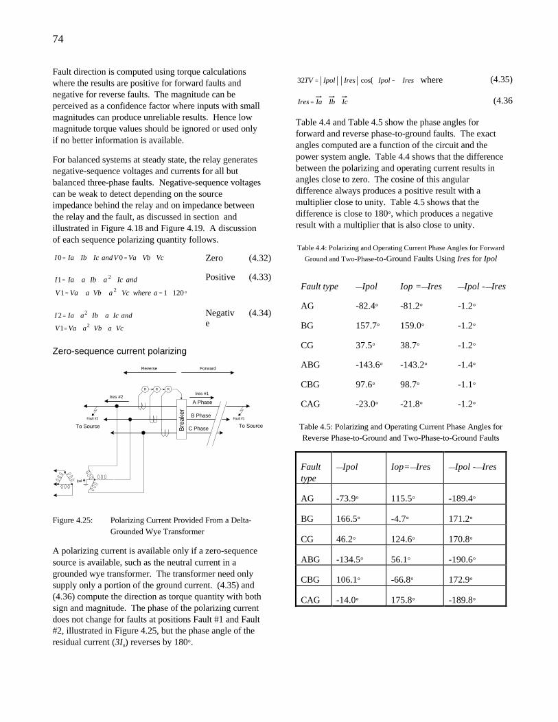
74
Fault direction is computed using torque calculations where the results are positive for forward faults and negative for reverse faults. The magnitude can be perceived as a confidence factor where inputs with small magnitudes can produce unreliable results. Hence low magnitude torque values should be ignored or used only if no better information is available.
For balanced systems at steady state, the relay generates negative-sequence voltages and currents for all but balanced three-phase faults. Negative-sequence voltages can be weak to detect depending on the source impedance behind the relay and on impedance between the relay and the fault, as discussed in section and illustrated in Figure 4.18 and Figure 4.19. A discussion of each sequence polarizing quantity follows.
VcVbVaVandIcIbIaI ++=++= 00 Zero (4.32)
°∠=⋅+⋅+=
⋅+⋅+=
12011
12
2
awhereVcaVbaVaV
andIcaIbaIaI
Positive (4.33)
VcaVbaVaV
andIcaIbaIaI
⋅+⋅+=
⋅+⋅+=
2
2
1
2
Negative
(4.34)
Zero-sequence current polarizing
Ipol
R R R
Bre
aker
To Source To Source
Fault #1
Ires #1
ForwardReverse
Fault #2
Ires #2
B Phase
A Phase
C Phase
Figure 4.25: Polarizing Current Provided From a Delta-Grounded Wye Transformer
A polarizing current is available only if a zero-sequence source is available, such as the neutral current in a grounded wye transformer. The transformer need only supply only a portion of the ground current. (4.35) and (4.36) compute the direction as torque quantity with both sign and magnitude. The phase of the polarizing current does not change for faults at positions Fault #1 and Fault #2, illustrated in Figure 4.25, but the phase angle of the residual current (3I0) reverses by 180°.
( )IresIpolIresIpolTV ∠−∠= cos32 where (4.35)
IcIbIaIres ++= (4.36
Table 4.4 and Table 4.5 show the phase angles for forward and reverse phase-to-ground faults. The exact angles computed are a function of the circuit and the power system angle. Table 4.4 shows that the difference between the polarizing and operating current results in angles close to zero. The cosine of this angular difference always produces a positive result with a multiplier close to unity. Table 4.5 shows that the difference is close to 180°, which produces a negative result with a multiplier that is also close to unity.
Table 4.4: Polarizing and Operating Current Phase Angles for Forward
Ground and Two-Phase-to-Ground Faults Using Ires for Ipol
Fault type ∠Ipol Iop =∠Ires ∠Ipol -∠Ires
AG -82.4° -81.2° -1.2°
BG 157.7° 159.0° -1.2°
CG 37.5° 38.7° -1.2°
ABG -143.6° -143.2° -1.4°
CBG 97.6° 98.7° -1.1°
CAG -23.0° -21.8° -1.2°
Table 4.5: Polarizing and Operating Current Phase Angles for Reverse Phase-to-Ground and Two-Phase-to-Ground Faults
Fault type
∠Ipol Iop=∠Ires ∠Ipol -∠Ires
AG -73.9° 115.5° -189.4°
BG 166.5° -4.7° 171.2°
CG 46.2° 124.6° 170.8°
ABG -134.5° 56.1° -190.6°
CBG 106.1° -66.8° 172.9°
CAG -14.0° 175.8° -189.8°
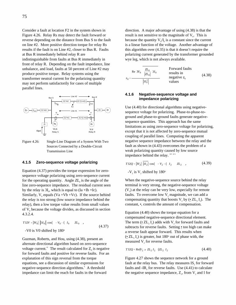
75
Consider a fault at location F2 in the system shown in Figure 4.26. Relay Rs may detect the fault forward or reverse depending on the distance from Bus S to the fault on line #2. More positive direction torque for relay Rs results if the fault is on Line #2, closer to Bus R. Faults at Bus R immediately behind relay R are indistinguishable from faults at Bus R immediately in front of relay R. Depending on the fault impedance, line unbalance, and load, faults at 50 percent of Line #2 may produce positive torque. Relay systems using the transformer neutral current for the polarizing quantity may not perform satisfactorily for cases of multiple parallel lines.
Rr
Vr,IrRelay R
Rs
Vs,IsRelay S
ZL*m2 ZL*(1-m2)
ZL*m1 ZL*(1-m1)
F2
Line #1
Line #2
Zt
ISpol
Es ZL*m3ZSRC
Bus S
ErZrr
Bus R
IrIs
IsREV IsFOR
Figure 4.26: Single-Line Diagram of a System With Two Sources Connected by a Double-Circuit Transmission Line
4.1.5 Zero-sequence voltage polarizing
Equation (4.37) provides the torque expression for zero-sequence voltage polarizing using zero-sequence current for the operating quantity. Angle ZL0 is the angle of the line zero-sequence impedance. The residual current seen by the relay is 3I0, which is equal to (Ia +Ib +Ic). Similarly, V0 equals (Va +Vb +Vc). If the source behind the relay is too strong (low source impedance behind the relay), then a low torque value results from small values of V0 because the voltage divides, as discussed in section 4.3.2.4.
( )( )00000 cos3332 ZLIVIVVT ∠+∠−−∠⋅⋅= ,
∠-V0 is V0 shifted by 180° (4.37)
Guzman, Roberts, and Hou, using (4.38), present an alternate directional algorithm based on zero-sequence voltage current.xi The result calculated for Z0 is negative for forward faults and positive for reverse faults. For an explanation of this sign reversal from the torque equations, see a discussion of similar expressions for negative-sequence direction algorithms.x A threshold impedance can limit the reach for faults in the forward
direction. A major advantage of using (4.38) is that the result is not sensitive to the magnitude of V0. This is because the quantity V0/I0 is a constant since the current is a linear function of the voltage. Another advantage of this algorithm over (4.35) is that it doesn’t require the polarizing current generated by the transformer grounded wye leg, which is not always available.
20
00
00
03
33Re
I
IZL
ZLV
z
⋅⋅
=
Forward faults results in negative z0 values
(4.38)
4.1.6 Negative-sequence voltage and impedance polarizing
Use (4.40) for directional algorithms using negative-sequence voltage for polarizing. Phase-to-phase-to-ground and phase-to-ground faults generate negative-sequence quantities. This approach has the same limitations as using zero-sequence voltage for polarizing, except that it is not affected by zero-sequence mutual coupling of parallel lines. Computing the apparent negative sequence impedance between the relay and the fault as shown in (4.43) overcomes the problem of a weak polarizing quantity caused by low source impedance behind the relay. xii xi x
( )( )22222 cos3332 ZLIVIVQT ∠+∠−−∠⋅⋅= ,
∠-V2 is V2 shifted by 180°
(4.39)
When the negative-sequence source behind the relay terminal is very strong, the negative-sequence voltage (V2) at the relay can be very low, especially for remote faults. To overcome low V2 magnitude, we can add a compensating quantity that boosts V2 by (•⋅ZL2⋅I2). The constant, •, controls the amount of compensation.
Equation (4.40) shows the torque equation for a compensated negative-sequence directional element. The term (•⋅ZL2⋅I2) adds with V2 for forward faults and subtracts for reverse faults. Setting • too high can make a reverse fault appear forward. This results when (•⋅ZL2⋅I2) is greater, but 180° out of phase with, the measured V2 for reverse faults.
( ) ( )22222Re32 IZLIZLVQT ⋅⋅⋅= α (4.40)
Figure 4.27 shows the sequence network for a ground fault at the relay bus. The relay measures IS2 for forward faults and -IR2 for reverse faults. Use (4.41) to calculate the negative sequence impedance, Z2, from V2 and I for
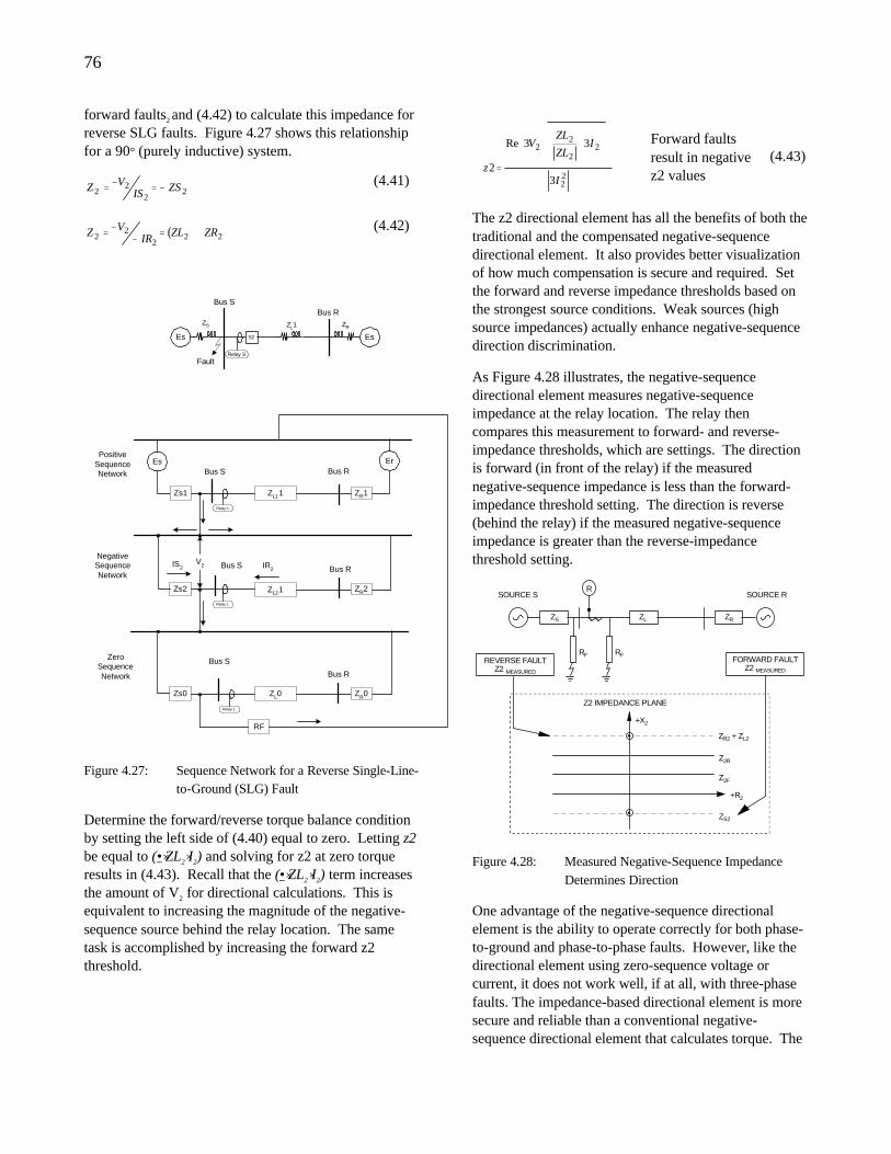
76
forward faults2 and (4.42) to calculate this impedance for reverse SLG faults. Figure 4.27 shows this relationship for a 90° (purely inductive) system.
22
22 ZSIS
VZ −=−
= (4.41)
( )222
22 ZRZLIR
VZ +=−
−= (4.42)
Fault
Bus S
Relay S
52
ZL1
Es
ZS
Es
ZR
Bus R
Es
Relay 1
Zs1
Bus S
ZL11 ZR1
Relay 1
Zs2
Bus S
ZL21
Relay 1
Zs0
Bus S
ZL0
PositiveSequenceNetwork
NegativeSequenceNetwork
ZeroSequenceNetwork
Bus R
Bus R
ZR2
V2 IR2IS2
RF
Er
Bus R
ZR0
Figure 4.27: Sequence Network for a Reverse Single-Line-to-Ground (SLG) Fault
Determine the forward/reverse torque balance condition by setting the left side of (4.40) equal to zero. Letting z2 be equal to (•⋅ZL2⋅I2) and solving for z2 at zero torque results in (4.43). Recall that the (•⋅ZL2⋅I2) term increases the amount of V2 for directional calculations. This is equivalent to increasing the magnitude of the negative-sequence source behind the relay location. The same task is accomplished by increasing the forward z2 threshold.
22
22
22
3
33Re
2I
IZL
ZLV
z
⋅⋅
=
Forward faults result in negative z2 values
(4.43)
The z2 directional element has all the benefits of both the traditional and the compensated negative-sequence directional element. It also provides better visualization of how much compensation is secure and required. Set the forward and reverse impedance thresholds based on the strongest source conditions. Weak sources (high source impedances) actually enhance negative-sequence direction discrimination.
As Figure 4.28 illustrates, the negative-sequence directional element measures negative-sequence impedance at the relay location. The relay then compares this measurement to forward- and reverse-impedance thresholds, which are settings. The direction is forward (in front of the relay) if the measured negative-sequence impedance is less than the forward-impedance threshold setting. The direction is reverse (behind the relay) if the measured negative-sequence impedance is greater than the reverse-impedance threshold setting.
SOURCE S SOURCE R
ZS ZL ZR
RF
Z2 IMPEDANCE PLANE
+X2
Z2R
Z2F
+R2
ZS2
FORWARD FAULTZ2 MEASURED
R
REVERSE FAULTZ2 MEASURED
ZR2 + ZL2
RF
Figure 4.28: Measured Negative-Sequence Impedance Determines Direction
One advantage of the negative-sequence directional element is the ability to operate correctly for both phase-to-ground and phase-to-phase faults. However, like the directional element using zero-sequence voltage or current, it does not work well, if at all, with three-phase faults. The impedance-based directional element is more secure and reliable than a conventional negative-sequence directional element that calculates torque. The
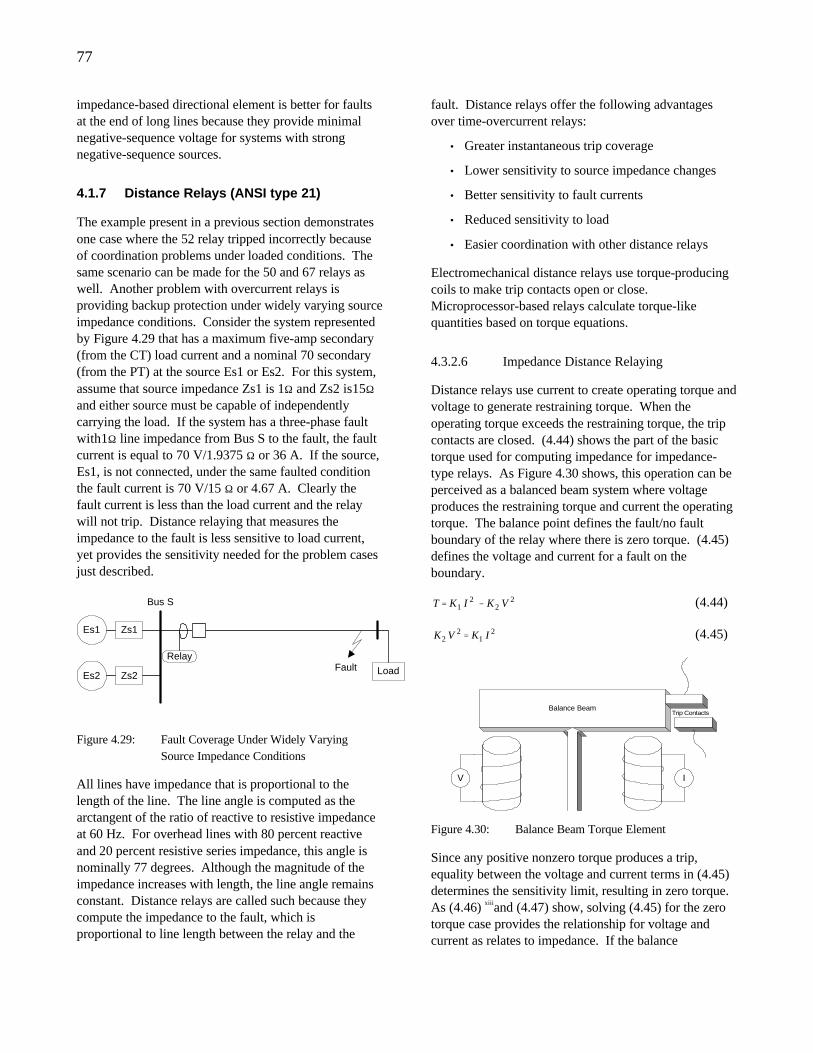
77
impedance-based directional element is better for faults at the end of long lines because they provide minimal negative-sequence voltage for systems with strong negative-sequence sources.
4.1.7 Distance Relays (ANSI type 21)
The example present in a previous section demonstrates one case where the 52 relay tripped incorrectly because of coordination problems under loaded conditions. The same scenario can be made for the 50 and 67 relays as well. Another problem with overcurrent relays is providing backup protection under widely varying source impedance conditions. Consider the system represented by Figure 4.29 that has a maximum five-amp secondary (from the CT) load current and a nominal 70 secondary (from the PT) at the source Es1 or Es2. For this system, assume that source impedance Zs1 is 1Ω and Zs2 is15Ω and either source must be capable of independently carrying the load. If the system has a three-phase fault with1Ω line impedance from Bus S to the fault, the fault current is equal to 70 V/1.9375 Ω or 36 A. If the source, Es1, is not connected, under the same faulted condition the fault current is 70 V/15 Ω or 4.67 A. Clearly the fault current is less than the load current and the relay will not trip. Distance relaying that measures the impedance to the fault is less sensitive to load current, yet provides the sensitivity needed for the problem cases just described.
Relay
LoadFault
Zs1Es1
Zs2Es2
Bus S
Figure 4.29: Fault Coverage Under Widely Varying Source Impedance Conditions
All lines have impedance that is proportional to the length of the line. The line angle is computed as the arctangent of the ratio of reactive to resistive impedance at 60 Hz. For overhead lines with 80 percent reactive and 20 percent resistive series impedance, this angle is nominally 77 degrees. Although the magnitude of the impedance increases with length, the line angle remains constant. Distance relays are called such because they compute the impedance to the fault, which is proportional to line length between the relay and the
fault. Distance relays offer the following advantages over time-overcurrent relays:
• Greater instantaneous trip coverage
• Lower sensitivity to source impedance changes
• Better sensitivity to fault currents
• Reduced sensitivity to load
• Easier coordination with other distance relays
Electromechanical distance relays use torque-producing coils to make trip contacts open or close. Microprocessor-based relays calculate torque-like quantities based on torque equations.
4.3.2.6 Impedance Distance Relaying
Distance relays use current to create operating torque and voltage to generate restraining torque. When the operating torque exceeds the restraining torque, the trip contacts are closed. (4.44) shows the part of the basic torque used for computing impedance for impedance-type relays. As Figure 4.30 shows, this operation can be perceived as a balanced beam system where voltage produces the restraining torque and current the operating torque. The balance point defines the fault/no fault boundary of the relay where there is zero torque. (4.45) defines the voltage and current for a fault on the boundary.
22
21 VKIKT −= (4.44)
21
22 IKVK = (4.45)
Balance Beam
V I
Trip Contacts
Figure 4.30: Balance Beam Torque Element
Since any positive nonzero torque produces a trip, equality between the voltage and current terms in (4.45) determines the sensitivity limit, resulting in zero torque. As (4.46) xiiiand (4.47) show, solving (4.45) for the zero torque case provides the relationship for voltage and current as relates to impedance. If the balance
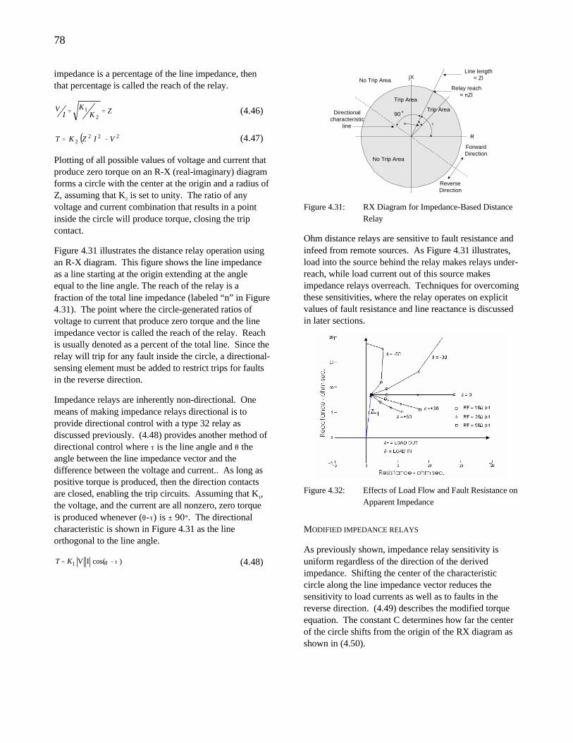
78
impedance is a percentage of the line impedance, then that percentage is called the reach of the relay.
ZKK
IV ==
21 (4.46)
( )2222 VIZKT −= (4.47)
Plotting of all possible values of voltage and current that produce zero torque on an R-X (real-imaginary) diagram forms a circle with the center at the origin and a radius of Z, assuming that K2 is set to unity. The ratio of any voltage and current combination that results in a point inside the circle will produce torque, closing the trip contact.
Figure 4.31 illustrates the distance relay operation using an R-X diagram. This figure shows the line impedance as a line starting at the origin extending at the angle equal to the line angle. The reach of the relay is a fraction of the total line impedance (labeled “n” in Figure 4.31). The point where the circle-generated ratios of voltage to current that produce zero torque and the line impedance vector is called the reach of the relay. Reach is usually denoted as a percent of the total line. Since the relay will trip for any fault inside the circle, a directional-sensing element must be added to restrict trips for faults in the reverse direction.
Impedance relays are inherently non-directional. One means of making impedance relays directional is to provide directional control with a type 32 relay as discussed previously. (4.48) provides another method of directional control where τ is the line angle and θ the angle between the line impedance vector and the difference between the voltage and current.. As long as positive torque is produced, then the direction contacts are closed, enabling the trip circuits. Assuming that K1, the voltage, and the current are all nonzero, zero torque is produced whenever (θ-τ) is ± 90°. The directional characteristic is shown in Figure 4.31 as the line orthogonal to the line angle.
)cos(IV1 τθ −= KT (4.48)
Line length= Zl
Relay reach= nZl
jX
R
Trip Area
No Trip Area
ForwardDirection
ReverseDirection
No Trip Area
Trip Area90 oDirectional
characteristicline τΘ
Figure 4.31: RX Diagram for Impedance-Based Distance Relay
Ohm distance relays are sensitive to fault resistance and infeed from remote sources. As Figure 4.31 illustrates, load into the source behind the relay makes relays under-reach, while load current out of this source makes impedance relays overreach. Techniques for overcoming these sensitivities, where the relay operates on explicit values of fault resistance and line reactance is discussed in later sections.
Figure 4.32: Effects of Load Flow and Fault Resistance on Apparent Impedance
MODIFIED IMPEDANCE RELAYS
As previously shown, impedance relay sensitivity is uniform regardless of the direction of the derived impedance. Shifting the center of the characteristic circle along the line impedance vector reduces the sensitivity to load currents as well as to faults in the reverse direction. (4.49) describes the modified torque equation. The constant C determines how far the center of the circle shifts from the origin of the RX diagram as shown in (4.50).
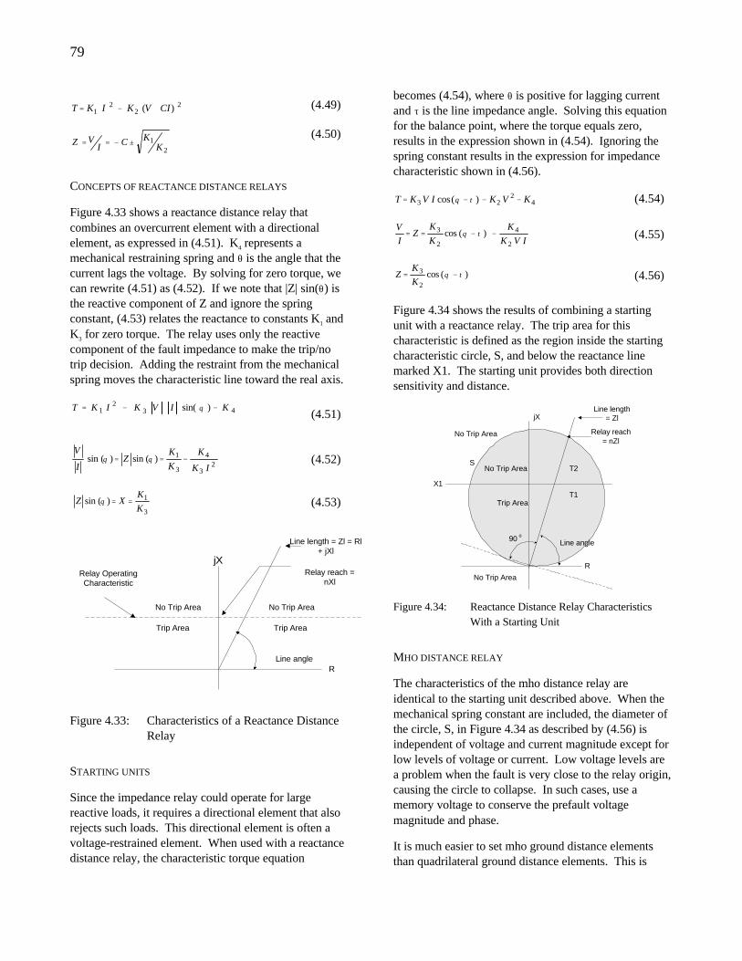
79
22
21 )( CIVKIKT +−= (4.49)
21
KKCI
VZ ±−== (4.50)
CONCEPTS OF REACTANCE DISTANCE RELAYS
Figure 4.33 shows a reactance distance relay that combines an overcurrent element with a directional element, as expressed in (4.51). K4 represents a mechanical restraining spring and θ is the angle that the current lags the voltage. By solving for zero torque, we can rewrite (4.51) as (4.52). If we note that |Z| sin(θ) is the reactive component of Z and ignore the spring constant, (4.53) relates the reactance to constants K1 and K3 for zero torque. The relay uses only the reactive component of the fault impedance to make the trip/no trip decision. Adding the restraint from the mechanical spring moves the characteristic line toward the real axis.
432
1 )sin( KIVKIKT −−= θ
(4.51)
23
4
3
1)(sin)(sinIK
K
K
KZ
I
V−== θθ (4.52)
3
1)(sinK
KXZ ==θ (4.53)
Line length = Zl = Rl+ jXl
Relay reach =nXl
Line angle
jX
R
Trip Area
Relay OperatingCharacteristic
No Trip Area
Trip Area
No Trip Area
Figure 4.33: Characteristics of a Reactance Distance Relay
STARTING UNITS
Since the impedance relay could operate for large reactive loads, it requires a directional element that also rejects such loads. This directional element is often a voltage-restrained element. When used with a reactance distance relay, the characteristic torque equation
becomes (4.54), where θ is positive for lagging current and τ is the line impedance angle. Solving this equation for the balance point, where the torque equals zero, results in the expression shown in (4.54). Ignoring the spring constant results in the expression for impedance characteristic shown in (4.56).
42
23 )(cos KVKIVKT −−−= τθ (4.54)
IVK
K
K
KZ
I
V
2
4
2
3 )(cos −−== τθ (4.55)
)(cos2
3 τθ −=K
KZ (4.56)
Figure 4.34 shows the results of combining a starting unit with a reactance relay. The trip area for this characteristic is defined as the region inside the starting characteristic circle, S, and below the reactance line marked X1. The starting unit provides both direction sensitivity and distance.
Line length= Zl
Relay reach= nZl
Line angle
jX
R
No Trip Area
No Trip Area
90 o
ST2
T1
X1
Trip Area
No Trip Area
Figure 4.34: Reactance Distance Relay Characteristics With a Starting Unit
MHO DISTANCE RELAY
The characteristics of the mho distance relay are identical to the starting unit described above. When the mechanical spring constant are included, the diameter of the circle, S, in Figure 4.34 as described by (4.56) is independent of voltage and current magnitude except for low levels of voltage or current. Low voltage levels are a problem when the fault is very close to the relay origin, causing the circle to collapse. In such cases, use a memory voltage to conserve the prefault voltage magnitude and phase.
It is much easier to set mho ground distance elements than quadrilateral ground distance elements. This is
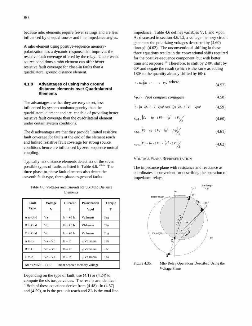
80
because mho elements require fewer settings and are less influenced by unequal source and line impedance angles.
A mho element using positive-sequence memory-polarization has a dynamic response that improves the resistive fault coverage offered by the relay. Under weak source conditions a mho element can offer better resistive fault coverage for close-in faults than a quadrilateral ground distance element.
4.1.8 Advantages of using mho ground distance elements over Quadralateral Elements
The advantages are that they are easy to set, less influenced by system nonhomogeneity than the quadrilateral element and are capable of providing better resistive fault coverage than the quadrilateral element under certain system conditions.
The disadvantages are that they provide limited resistive fault coverage for faults at the end of the element reach and limited resistive fault coverage for strong source conditions hence are influenced by zero-sequence mutual coupling.
Typically, six distance elements detect six of the seven possible types of faults as listed in Table 4.6. viii,xiv The three phase-to-phase fault elements also detect the seventh fault type, three-phase-to-ground faults.
Table 4.6: Voltages and Currents for Six Mho Distance Elements
Fault
Type
Voltage
V
Current
I
Polarization
Vpol
Torque
T
A to Gnd Va Ia + k0 Ir Va1mem Tag
B to Gnd Vb Ib + k0 Ir Vb1mem Tbg
C to Gnd Vc Ic + k0 Ir Vc1mem Tcg
A to B Va – Vb Ia – Ib -j Vc1mem Tab
B to C Vb – Vc Ib – Ic -j Va1mem Tbc
C to A Vc – Va Ic – Ia -j Vb1mem Tca
K0 = (Z0/Z1 – 1)/3 mem denotes memory voltage
Depending on the type of fault, use (4.1) or (4.24) to compute the six torque values. The results are identical. ix Both of these equations derive from (4.48). In (4.57) and (4.59), m is the per-unit reach and ZL is the total line
impedance. Table 4.6 defines variables V, I, and Vpol. As discussed in section 4.6.1.2, a voltage memory circuit generates the polarizing voltages described by (4.60) through (4.62). The unconventional shifting in these three equations results in the conventional shifts required for the positive-sequence component, but with better transient response. viii Therefore, to shift by 240°, shift by 60° and negate the result (which is the same as adding 180° to the quantity already shifted by 60°).
( )[ VpolVIZLmT ⋅−⋅⋅= Re
where (4.57)
=Vpol Vpol complex conjugate (4.58)
( )( )VpolVIZLmVpolVIZLmT ∠−⋅⋅∠−⋅⋅= cos (4.59)
( ) ( )[ ]3
1112 VcaVbaVaVa −−−−
= (4.60)
( ) ( )[ ]3
1112 VaaVcaVbVb −−−−
= (4.61)
( ) ( )[ ]3
1112 VbaVaaVcVc −−−−
= (4.62)
VOLTAGE PLANE REPRESENTATION
The impedance plane with resistance and reactance as coordinates is convenient for describing the operation of impedance relays.
(m Z
L) I
Line length= Zl
Relay reach
Line angle
Im
Re
V
δV90 o
M
O
Vpol
S
Figure 4.35: Mho Relay Operations Described Using the Voltage Plane
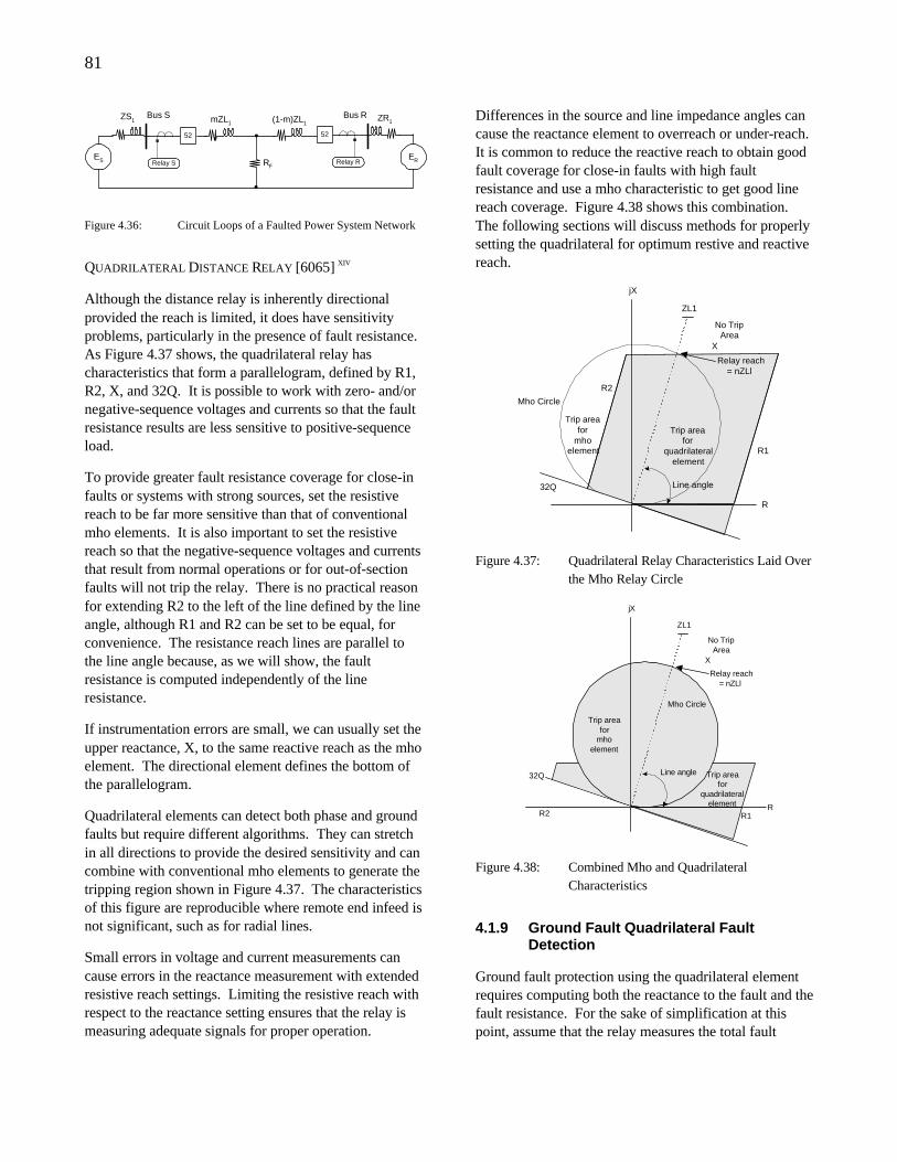
81
Bus S
52
mZL1
ES
ZS1
ER
ZR1Bus R
52
(1-m)ZL1
Relay S Relay RRF
Figure 4.36: Circuit Loops of a Faulted Power System Network
QUADRILATERAL DISTANCE RELAY [6065] XIV
Although the distance relay is inherently directional provided the reach is limited, it does have sensitivity problems, particularly in the presence of fault resistance. As Figure 4.37 shows, the quadrilateral relay has characteristics that form a parallelogram, defined by R1, R2, X, and 32Q. It is possible to work with zero- and/or negative-sequence voltages and currents so that the fault resistance results are less sensitive to positive-sequence load.
To provide greater fault resistance coverage for close-in faults or systems with strong sources, set the resistive reach to be far more sensitive than that of conventional mho elements. It is also important to set the resistive reach so that the negative-sequence voltages and currents that result from normal operations or for out-of-section faults will not trip the relay. There is no practical reason for extending R2 to the left of the line defined by the line angle, although R1 and R2 can be set to be equal, for convenience. The resistance reach lines are parallel to the line angle because, as we will show, the fault resistance is computed independently of the line resistance.
If instrumentation errors are small, we can usually set the upper reactance, X, to the same reactive reach as the mho element. The directional element defines the bottom of the parallelogram.
Quadrilateral elements can detect both phase and ground faults but require different algorithms. They can stretch in all directions to provide the desired sensitivity and can combine with conventional mho elements to generate the tripping region shown in Figure 4.37. The characteristics of this figure are reproducible where remote end infeed is not significant, such as for radial lines.
Small errors in voltage and current measurements can cause errors in the reactance measurement with extended resistive reach settings. Limiting the resistive reach with respect to the reactance setting ensures that the relay is measuring adequate signals for proper operation.
Differences in the source and line impedance angles can cause the reactance element to overreach or under-reach. It is common to reduce the reactive reach to obtain good fault coverage for close-in faults with high fault resistance and use a mho characteristic to get good line reach coverage. Figure 4.38 shows this combination. The following sections will discuss methods for properly setting the quadrilateral for optimum restive and reactive reach.
Line angle
jX
R
No TripArea
Trip areafor
quadrilateralelement
X
32Q
R2
R1
Mho Circle
Relay reach= nZLl
ZL1
Trip areafor
mhoelement
Figure 4.37: Quadrilateral Relay Characteristics Laid Over the Mho Relay Circle
Line angle
jX
R
No TripArea
X
32Q
R2 R1
Mho Circle
Relay reach= nZLl
ZL1
Trip areafor
quadrilateralelement
Trip areafor
mhoelement
Figure 4.38: Combined Mho and Quadrilateral Characteristics
4.1.9 Ground Fault Quadrilateral Fault Detection
Ground fault protection using the quadrilateral element requires computing both the reactance to the fault and the fault resistance. For the sake of simplification at this point, assume that the relay measures the total fault
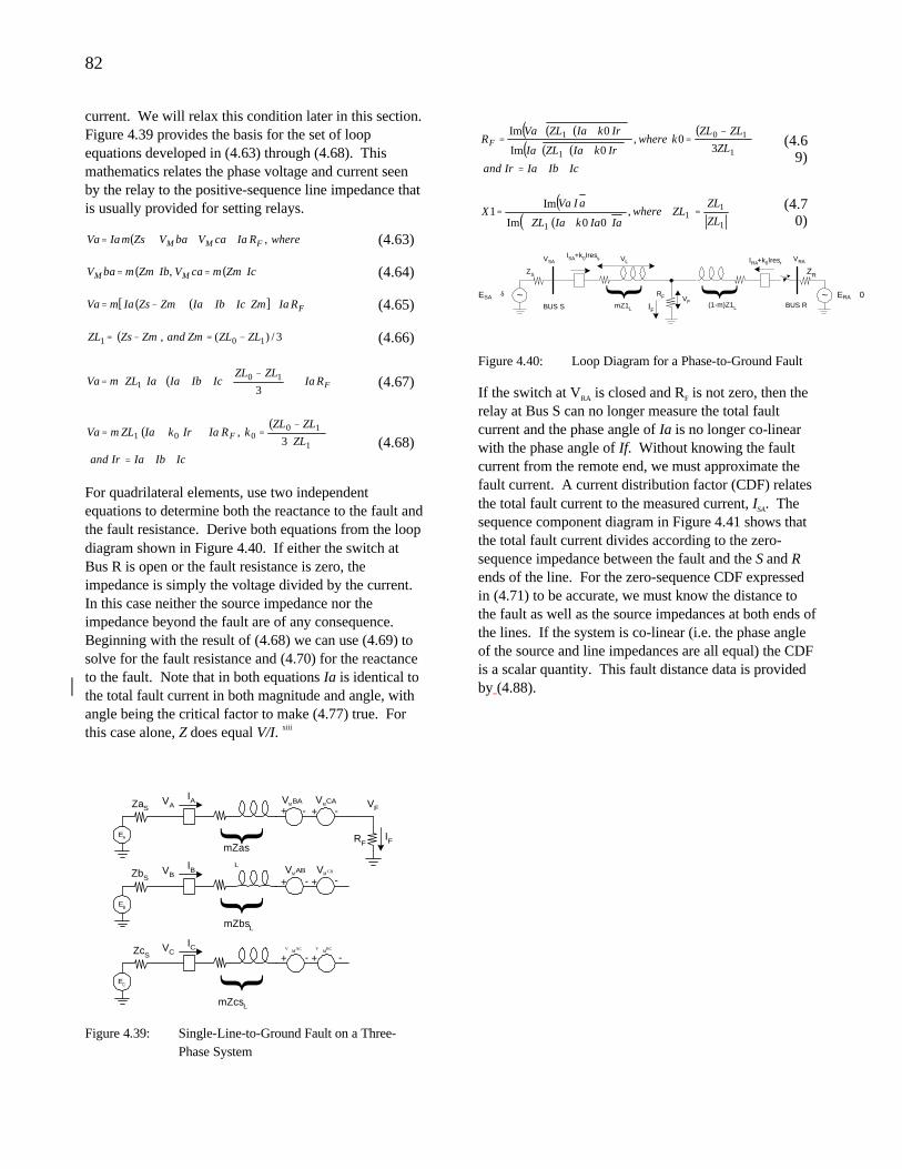
82
current. We will relax this condition later in this section. Figure 4.39 provides the basis for the set of loop equations developed in (4.63) through (4.68). This mathematics relates the phase voltage and current seen by the relay to the positive-sequence line impedance that is usually provided for setting relays.
( ) whereRIacaVbaVZsmIaVa FMM ,+++= (4.63)
( ) ( )IcZmmcaVIbZmmbaV MM == , (4.64)
( ) ( )[ ] FRIaZmIcIbIaZmZsIamVa ++++−= (4.65)
( ) 3/)(, 101 ZLZLZmandZmZsZL −=−= (4.66)
( ) FRIaZLZL
IcIbIaIaZLmVa +
−+++=
310
1 (4.67)
( ) ( )
IcIbIaIrand
ZL
ZLZLkRIaIrkIaZLmVa F
++=
⋅
−=++=
1
10001 3
, (4.68)
For quadrilateral elements, use two independent equations to determine both the reactance to the fault and the fault resistance. Derive both equations from the loop diagram shown in Figure 4.40. If either the switch at Bus R is open or the fault resistance is zero, the impedance is simply the voltage divided by the current. In this case neither the source impedance nor the impedance beyond the fault are of any consequence. Beginning with the result of (4.68) we can use (4.69) to solve for the fault resistance and (4.70) for the reactance to the fault. Note that in both equations Ia is identical to the total fault current in both magnitude and angle, with angle being the critical factor to make (4.77) true. For this case alone, Z does equal V/I. xiii
RF
VF
IFEA
mZas
L
IAVAZaS
EB
mZbsL
IBVBZbS
EC
mZcsL
ICVCZcS
+ +
+ +
+ + --
- -
- -VMBA VMCA
VMAB VM CB
VM
AC VM
BC
Figure 4.39: Single-Line-to-Ground Fault on a Three-Phase System
( )( )( )( )( )( )
( )
IcIbIaIrand
ZL
ZLZLkwhere
IrkIaZLIa
IrkIaZLVaRF
++=
−=
+⋅⋅
+⋅⋅=
1
10
1
1
30,
0Im
0Im
(4.69)
( )( )( ) 1
11
1
,00Im
Im1
ZL
ZLZLwhere
IaIakIaZL
aIVaX =∠
+∠= (4.7
0)
RF~
ISA+k0IressVSA
ZS
~
VRA
mZ1L(1-m)Z1L
ZR
IF
IRA+k0Iresr
VF
VL
ESA ∠ δ ERA ∠0 BUS S BUS R
Figure 4.40: Loop Diagram for a Phase-to-Ground Fault
If the switch at VRA is closed and RF is not zero, then the relay at Bus S can no longer measure the total fault current and the phase angle of Ia is no longer co-linear with the phase angle of If. Without knowing the fault current from the remote end, we must approximate the fault current. A current distribution factor (CDF) relates the total fault current to the measured current, ISA. The sequence component diagram in Figure 4.41 shows that the total fault current divides according to the zero-sequence impedance between the fault and the S and R ends of the line. For the zero-sequence CDF expressed in (4.71) to be accurate, we must know the distance to the fault as well as the source impedances at both ends of the lines. If the system is co-linear (i.e. the phase angle of the source and line impedances are all equal) the CDF is a scalar quantity. This fault distance data is provided by (4.88).
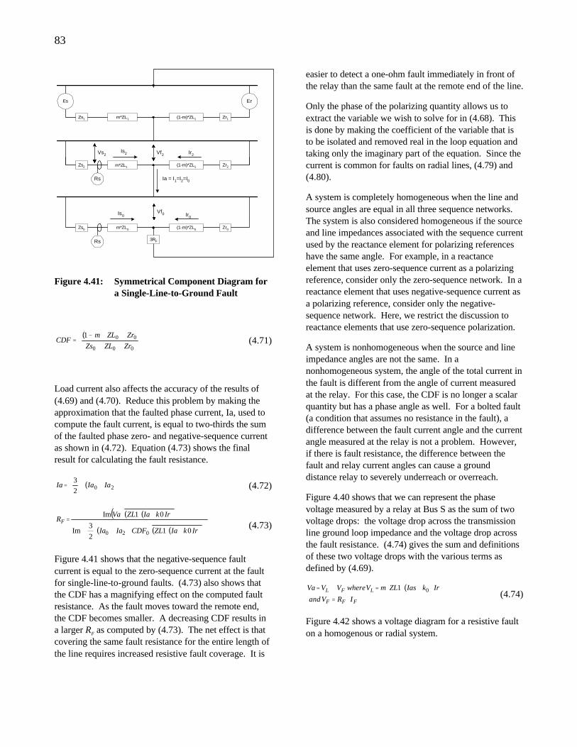
83
Rs
Es
Zs1 m*ZL1 (1-m)*ZL1 Zr1
Er
Zs2 (1-m)*ZL1 Zr2
Vs2
Ia = I1=I2=I0
m*ZL1
Rs
m*ZL0 (1-m)*ZL0 Zr0
3RF
Zs0
Vf2
Vf0
Is2
Is0
Ir2
Ir0
Figure 4.41: Symmetrical Component Diagram for a Single-Line-to-Ground Fault
( )
++
+⋅−=
000
001
ZrZLZs
ZrZLmCDF (4.71)
Load current also affects the accuracy of the results of (4.69) and (4.70). Reduce this problem by making the approximation that the faulted phase current, Ia, used to compute the fault current, is equal to two-thirds the sum of the faulted phase zero- and negative-sequence current as shown in (4.72). Equation (4.73) shows the final result for calculating the fault resistance.
( )202
3IaIaIa +⋅
= (4.72)
( )( )( )( ) ( )( )
+⋅⋅⋅+
+⋅⋅=
IrkIaZLCDFIaIa
IrkIaZLVaRF
012
3Im
01Im
020
(4.73)
Figure 4.41 shows that the negative-sequence fault current is equal to the zero-sequence current at the fault for single-line-to-ground faults. (4.73) also shows that the CDF has a magnifying effect on the computed fault resistance. As the fault moves toward the remote end, the CDF becomes smaller. A decreasing CDF results in a larger RF as computed by (4.73). The net effect is that covering the same fault resistance for the entire length of the line requires increased resistive fault coverage. It is
easier to detect a one-ohm fault immediately in front of the relay than the same fault at the remote end of the line.
Only the phase of the polarizing quantity allows us to extract the variable we wish to solve for in (4.68). This is done by making the coefficient of the variable that is to be isolated and removed real in the loop equation and taking only the imaginary part of the equation. Since the current is common for faults on radial lines, (4.79) and (4.80).
A system is completely homogeneous when the line and source angles are equal in all three sequence networks. The system is also considered homogeneous if the source and line impedances associated with the sequence current used by the reactance element for polarizing references have the same angle. For example, in a reactance element that uses zero-sequence current as a polarizing reference, consider only the zero-sequence network. In a reactance element that uses negative-sequence current as a polarizing reference, consider only the negative-sequence network. Here, we restrict the discussion to reactance elements that use zero-sequence polarization.
A system is nonhomogeneous when the source and line impedance angles are not the same. In a nonhomogeneous system, the angle of the total current in the fault is different from the angle of current measured at the relay. For this case, the CDF is no longer a scalar quantity but has a phase angle as well. For a bolted fault (a condition that assumes no resistance in the fault), a difference between the fault current angle and the current angle measured at the relay is not a problem. However, if there is fault resistance, the difference between the fault and relay current angles can cause a ground distance relay to severely underreach or overreach.
Figure 4.40 shows that we can represent the phase voltage measured by a relay at Bus S as the sum of two voltage drops: the voltage drop across the transmission line ground loop impedance and the voltage drop across the fault resistance. (4.74) gives the sum and definitions of these two voltage drops with the various terms as defined by (4.69).
( )
FFF
LFL
IRVand
IrkIasZLmVwhereVVVa
⋅=
⋅+⋅⋅=+= 01 (4.74)
Figure 4.42 shows a voltage diagram for a resistive fault on a homogenous or radial system.
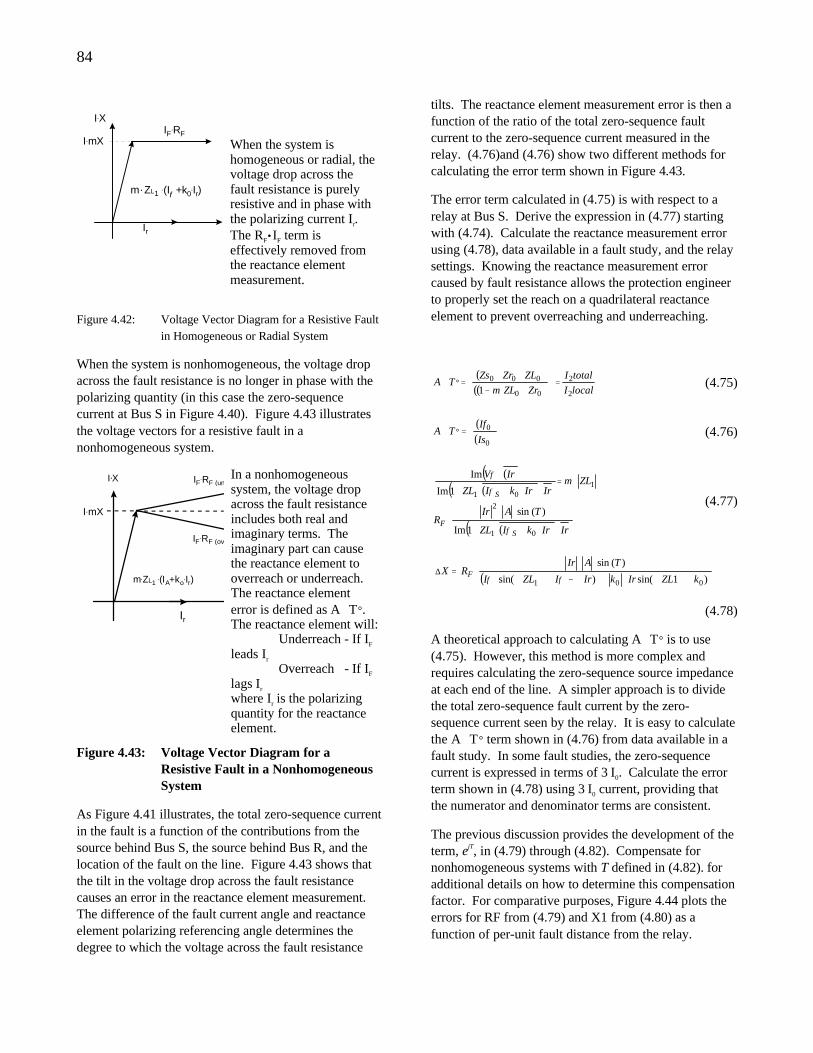
84
IF.RF
m . ZL1.(Iφφ +k0
.Ir)
Ir
I X.
I mX.
When the system is homogeneous or radial, the voltage drop across the fault resistance is purely resistive and in phase with the polarizing current Ir. The RF•IF term is effectively removed from the reactance element measurement.
Figure 4.42: Voltage Vector Diagram for a Resistive Fault in Homogeneous or Radial System
When the system is nonhomogeneous, the voltage drop across the fault resistance is no longer in phase with the polarizing quantity (in this case the zero-sequence current at Bus S in Figure 4.40). Figure 4.43 illustrates the voltage vectors for a resistive fault in a nonhomogeneous system.
IF.RF (underreach)
IF.RF (overreach)
Ir
I.X
m.Z 1.(IA+ko
.Ir)L
I mX.
In a nonhomogeneous system, the voltage drop across the fault resistance includes both real and imaginary terms. The imaginary part can cause the reactance element to overreach or underreach. The reactance element error is defined as A∠T°. The reactance element will: Underreach - If IF leads Ir
Overreach - If IF lags Ir
where Ir is the polarizing quantity for the reactance element.
Figure 4.43: Voltage Vector Diagram for a Resistive Fault in a Nonhomogeneous System
As Figure 4.41 illustrates, the total zero-sequence current in the fault is a function of the contributions from the source behind Bus S, the source behind Bus R, and the location of the fault on the line. Figure 4.43 shows that the tilt in the voltage drop across the fault resistance causes an error in the reactance element measurement. The difference of the fault current angle and reactance element polarizing referencing angle determines the degree to which the voltage across the fault resistance
tilts. The reactance element measurement error is then a function of the ratio of the total zero-sequence fault current to the zero-sequence current measured in the relay. (4.76)and (4.76) show two different methods for calculating the error term shown in Figure 4.43.
The error term calculated in (4.75) is with respect to a relay at Bus S. Derive the expression in (4.77) starting with (4.74). Calculate the reactance measurement error using (4.78), data available in a fault study, and the relay settings. Knowing the reactance measurement error caused by fault resistance allows the protection engineer to properly set the reach on a quadrilateral reactance element to prevent overreaching and underreaching.
( )( )( ) localI
totalI
ZrZLm
ZLZrZsTA
2
2
00
000
1=
+−
++=°∠ (4.75)
( )( )
=°∠
0
0
Is
IfTA (4.76)
( )( )( )( )
( )( )IrIrkIZL
TAIrR
ZLmIrIrkIZL
IrV
SF
S
⋅⋅+⋅∠
⋅⋅⋅
+⋅=⋅⋅+⋅∠
⋅
01
2
101
1Im
)(sin
1Im
Im
φ
φ
φ
(4.77)
( )
∠+∠⋅+∠−∠+∠⋅
⋅⋅=∆
)1sin()sin(
)(sin
001 kZLIrkIrIZLI
TAIrRX F
φφ
(4.78)
A theoretical approach to calculating A∠T° is to use (4.75). However, this method is more complex and requires calculating the zero-sequence source impedance at each end of the line. A simpler approach is to divide the total zero-sequence fault current by the zero-sequence current seen by the relay. It is easy to calculate the A∠T° term shown in (4.76) from data available in a fault study. In some fault studies, the zero-sequence current is expressed in terms of 3⋅I0. Calculate the error term shown in (4.78) using 3⋅I0 current, providing that the numerator and denominator terms are consistent.
The previous discussion provides the development of the term, ejT, in (4.79) through (4.82). Compensate for nonhomogeneous systems with T defined in (4.82). for additional details on how to determine this compensation factor. For comparative purposes, Figure 4.44 plots the errors for RF from (4.79) and X1 from (4.80) as a function of per-unit fault distance from the relay.
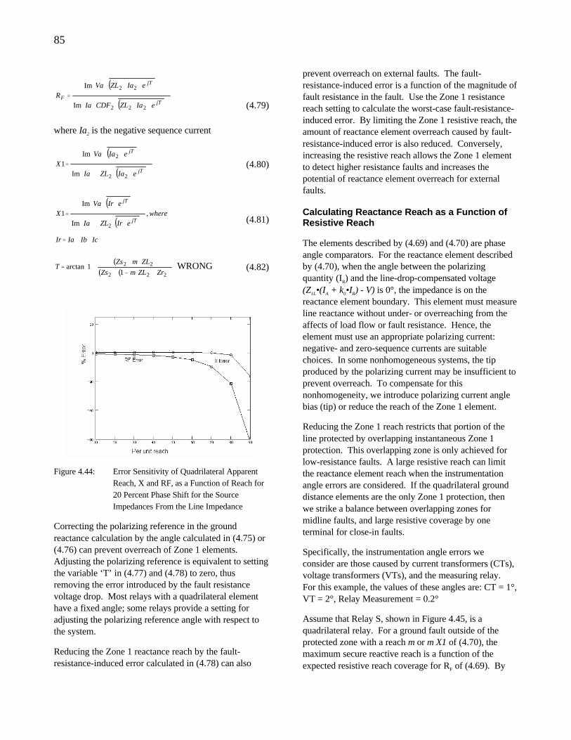
85
( )
( )
⋅⋅⋅⋅
⋅⋅⋅
=jT
jT
F
eIaZLCDFIa
eIaZLVaR
222
22
Im
Im
where Ia2 is the negative sequence current
(4.79)
( )
( )
⋅⋅∠⋅
⋅⋅
=jT
jT
eIaZLIa
eIaVaX
22
2
Im
Im1 (4.80)
( )
( )IcIbIaIr
whereeIrZLIa
eIrVaX
jT
jT
++=
⋅⋅∠⋅
⋅⋅
= ,Im
Im1
2 (4.81)
( )( )( )
+−+
⋅⋅+=
222
22
11arctan
ZrZLmZs
ZLmZsT WRONG (4.82)
Figure 4.44: Error Sensitivity of Quadrilateral Apparent Reach, X and RF, as a Function of Reach for 20 Percent Phase Shift for the Source Impedances From the Line Impedance
Correcting the polarizing reference in the ground reactance calculation by the angle calculated in (4.75) or (4.76) can prevent overreach of Zone 1 elements. Adjusting the polarizing reference is equivalent to setting the variable ‘T’ in (4.77) and (4.78) to zero, thus removing the error introduced by the fault resistance voltage drop. Most relays with a quadrilateral element have a fixed angle; some relays provide a setting for adjusting the polarizing reference angle with respect to the system.
Reducing the Zone 1 reactance reach by the fault-resistance-induced error calculated in (4.78) can also
prevent overreach on external faults. The fault-resistance-induced error is a function of the magnitude of fault resistance in the fault. Use the Zone 1 resistance reach setting to calculate the worst-case fault-resistance-induced error. By limiting the Zone 1 resistive reach, the amount of reactance element overreach caused by fault-resistance-induced error is also reduced. Conversely, increasing the resistive reach allows the Zone 1 element to detect higher resistance faults and increases the potential of reactance element overreach for external faults.
Calculating Reactance Reach as a Function of Resistive Reach
The elements described by (4.69) and (4.70) are phase angle comparators. For the reactance element described by (4.70), when the angle between the polarizing quantity (IR) and the line-drop-compensated voltage (Z1L•(IA + k0•IR) - V) is 0°, the impedance is on the reactance element boundary. This element must measure line reactance without under- or overreaching from the affects of load flow or fault resistance. Hence, the element must use an appropriate polarizing current: negative- and zero-sequence currents are suitable choices. In some nonhomogeneous systems, the tip produced by the polarizing current may be insufficient to prevent overreach. To compensate for this nonhomogeneity, we introduce polarizing current angle bias (tip) or reduce the reach of the Zone 1 element.
Reducing the Zone 1 reach restricts that portion of the line protected by overlapping instantaneous Zone 1 protection. This overlapping zone is only achieved for low-resistance faults. A large resistive reach can limit the reactance element reach when the instrumentation angle errors are considered. If the quadrilateral ground distance elements are the only Zone 1 protection, then we strike a balance between overlapping zones for midline faults, and large resistive coverage by one terminal for close-in faults.
Specifically, the instrumentation angle errors we consider are those caused by current transformers (CTs), voltage transformers (VTs), and the measuring relay. For this example, the values of these angles are: CT = 1°, VT = 2°, Relay Measurement = 0.2°
Assume that Relay S, shown in Figure 4.45, is a quadrilateral relay. For a ground fault outside of the protected zone with a reach m or m X1 of (4.70), the maximum secure reactive reach is a function of the expected resistive reach coverage for RF of (4.69). By
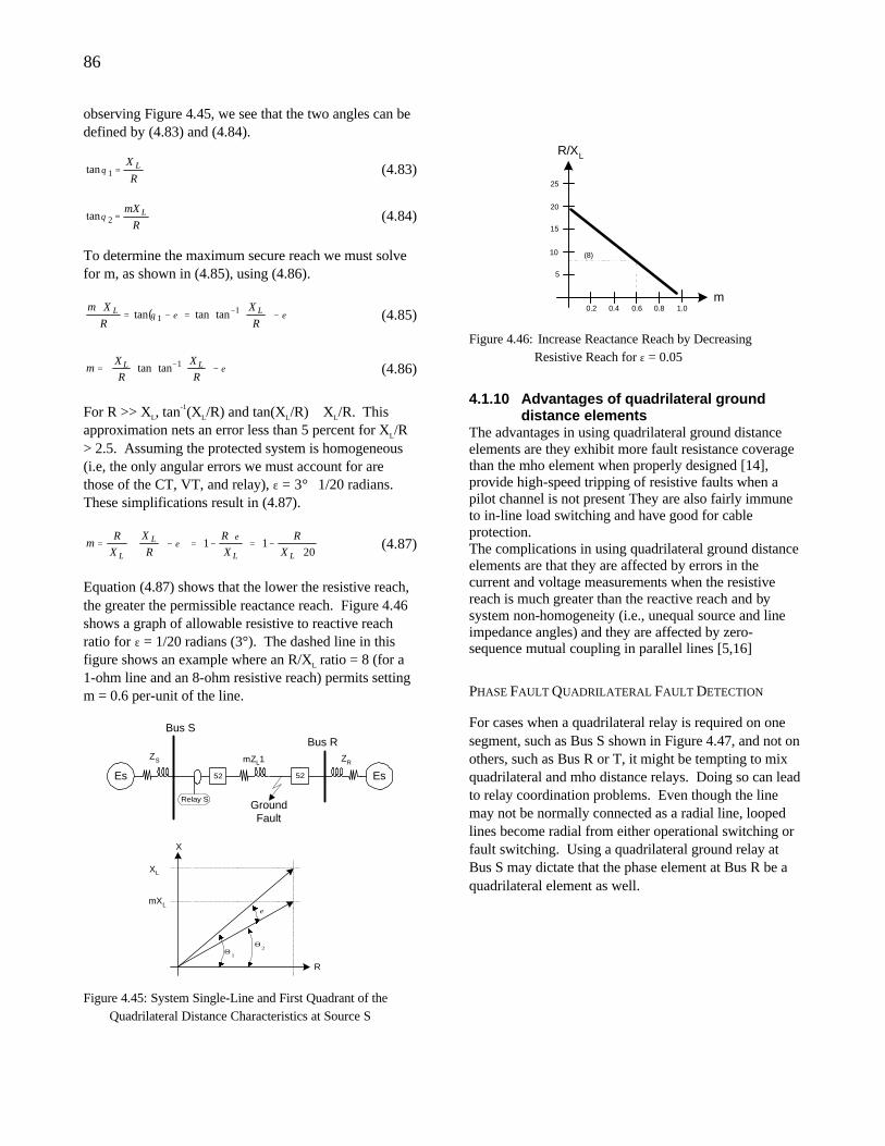
86
observing Figure 4.45, we see that the two angles can be defined by (4.83) and (4.84).
R
X L=1tan θ (4.83)
R
mX L=2tanθ (4.84)
To determine the maximum secure reach we must solve for m, as shown in (4.85), using (4.86).
( )
−
=−=
⋅ − εεθR
X
R
Xm LL 11 tantantan (4.85)
−
= − ε
R
X
R
Xm LL 1tantan (4.86)
For R >> XL, tan-1(XL/R) and tan(XL/R) ≅ XL/R. This approximation nets an error less than 5 percent for XL/R > 2.5. Assuming the protected system is homogeneous (i.e, the only angular errors we must account for are those of the CT, VT, and relay), ε = 3°≅ 1/20 radians. These simplifications result in (4.87).
⋅−=
⋅−=
−
=
2011
LL
L
L X
R
X
R
R
X
X
Rm
εε (4.87)
Equation (4.87) shows that the lower the resistive reach, the greater the permissible reactance reach. Figure 4.46 shows a graph of allowable resistive to reactive reach ratio for ε = 1/20 radians (3°). The dashed line in this figure shows an example where an R/XL ratio = 8 (for a 1-ohm line and an 8-ohm resistive reach) permits setting m = 0.6 per-unit of the line.
GroundFault
Bus S
52
mZL1
Es
ZS
Es
ZR
Bus R
52
X
R
XL
mXLε
Θ1
Θ2
Relay S
Figure 4.45: System Single-Line and First Quadrant of the Quadrilateral Distance Characteristics at Source S
m
R/XL
0.2 0.4 0.6 0.8 1.0
5
10
15
20
25
(8)
Figure 4.46: Increase Reactance Reach by Decreasing Resistive Reach for ε = 0.05
4.1.10 Advantages of quadrilateral ground distance elements
The advantages in using quadrilateral ground distance elements are they exhibit more fault resistance coverage than the mho element when properly designed [14], provide high-speed tripping of resistive faults when a pilot channel is not present They are also fairly immune to in-line load switching and have good for cable protection. The complications in using quadrilateral ground distance elements are that they are affected by errors in the current and voltage measurements when the resistive reach is much greater than the reactive reach and by system non-homogeneity (i.e., unequal source and line impedance angles) and they are affected by zero-sequence mutual coupling in parallel lines [5,16]
PHASE FAULT QUADRILATERAL FAULT DETECTION
For cases when a quadrilateral relay is required on one segment, such as Bus S shown in Figure 4.47, and not on others, such as Bus R or T, it might be tempting to mix quadrilateral and mho distance relays. Doing so can lead to relay coordination problems. Even though the line may not be normally connected as a radial line, looped lines become radial from either operational switching or fault switching. Using a quadrilateral ground relay at Bus S may dictate that the phase element at Bus R be a quadrilateral element as well.
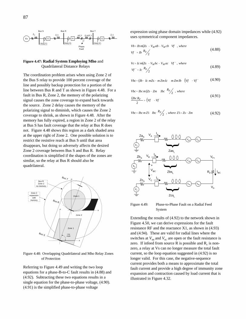
87
Relay RRelay R
PhaseFault
Bus S
Relay S
ZL1
Es
ZS
Bus R
mZL1
52 52
ZL1
Bus T
52
(1-m)ZL1
Figure 4.47: Radial System Employing Mho and Quadrilateral Distance Relays
The coordination problem arises when using Zone 2 of the Bus S relay to provide 100 percent coverage of the line and possibly backup protection for a portion of the line between Bus R and T as shown in Figure 4.48. For a fault in Bus R, Zone 2, the memory of the polarizing signal causes the zone coverage to expand back towards the source. Zone 2 delay causes the memory of the polarizing signal to diminish, which causes the Zone 2 coverage to shrink, as shown in Figure 4.48. After the memory has fully expired, a region in Zone 2 of the relay at Bus S has fault coverage that the relay at Bus R does not. Figure 4.48 shows this region as a dark shaded area at the upper right of Zone 2. One possible solution is to restrict the resistive reach at Bus S until that area disappears, but doing so adversely affects the desired Zone 2 coverage between Bus S and Bus R. Relay coordination is simplified if the shapes of the zones are similar, so the relay at Bus R should also be quadrilateral.
Bus S Lineangle
jX
R
jX
R
Bus R
Zone 1
Zone 1
Zone 2
Bus RZone 2
no memory
Bus T
Zone 2expansion
withmemory
Figure 4.48: Overlapping Quadrilateral and Mho Relay Zones of Protection
Referring to Figure 4.49 and writing the two loop equations for a phase-B-to-C fault results in (4.88) and (4.92). Subtracting these two equations results in a single equation for the phase-to-phase voltage, (4.90). (4.91) is the simplified phase-to-phase voltage
expression using phase domain impedances while (4.92) uses symmetrical component impedances.
( )
2
,
F
MM
RIbVf
whereVfcbVabVZsmIbVb
⋅=
+−−=
+
+
(4.88)
( )
2
,
F
MM
RIcVf
whereVfacVbcVZsmIcVc
⋅=
+−−=
−
−
(4.89)
( ) ( )−+ −++−−= VfVfIbZmmIcZmmmZsIcIbVbc (4.90)
( )
( ) ( )−+ −=
+−=
VfVfRIbc
whereRIbcZmZsmIbcVbc
F
F
2
,2 (4.91)
ZmZsZwhereRIbcZmIbcVbc F −=
+= 1,21 (4.92)
RF
VF+
IBC
EA
ZasL
IAVAZaS
EB
ZbsL
IBVBZbS
EC
ZcsL
ICVCZcS
VBA
VAB
VAC
VCA
VCB
VBC
VF-
VBC
+
-
Figure 4.49: Phase-to-Phase Fault on a Radial Feed System
Extending the results of (4.92) to the network shown in Figure 4.50, we can derive expressions for the fault resistance RF and the reactance X1, as shown in (4.93) and (4.94). These are valid for radial lines where the switches at VRB and VRC are open or the fault resistance is zero. If infeed from source R is possible and RF is non-zero, a relay at Vs can no longer measure the total fault current, so the loop equation suggested in (4.92) is no longer valid. For this case, the negative-sequence current provides both a means to approximate the total fault current and provide a high degree of immunity zone expansion and contraction caused by load current that is illustrated in Figure 4.32.
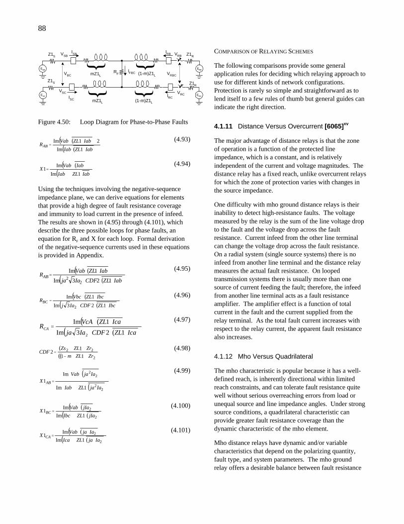
88
ESB
RF
ISBVSBZ1S
IFBC
ESC
VSC
VBC
ERB
IRB VRB
ERC
Z1R
VRCIRC
VRBC
mZ1L
ISC (1-m)Z1L
mZ1L(1-m)Z1L
Z1S
Z1R
Figure 4.50: Loop Diagram for Phase-to-Phase Faults
( )( )( )( )IabZLIab
IabZLVabRAB
⋅⋅
⋅⋅⋅=
1Im
21Im (4.93)
( )( )( )IabZLIab
IabVabX
⋅∠⋅
⋅=
1Im
Im1
(4.94)
Using the techniques involving the negative-sequence impedance plane, we can derive equations for elements that provide a high degree of fault resistance coverage and immunity to load current in the presence of infeed. The results are shown in (4.95) through (4.101), which describe the three possible loops for phase faults, an equation for RF and X for each loop. Formal derivation of the negative-sequence currents used in these equations is provided in Appendix.
( )( )( )( )IabZLCDFIaja
IabZLVabRAB
⋅⋅⋅
⋅⋅=
123Im
1Im
22
(4.95)
( )( )( )( )IbcZLCDFIaj
IbcZLVbcRBC
⋅⋅⋅
⋅⋅=
123Im
1Im
2
(4.96)
( )( )( )( )IcaZLCDFIaja
IcaZLVcARCA
⋅⋅⋅
⋅⋅=
123Im
1Im
2
(4.97)
( )( )( )2
22
11
12
ZrZLm
ZrZLZsCDF
+⋅−
++= (4.98)
( )
( )
⋅∠⋅
⋅
=
22
22
1Im
Im1
IajaZLIab
IajaVabX AB
(4.99)
( )( )( )( )2
2
1Im
Im1
jIaZLIbc
jIaVabX BC
⋅∠⋅
⋅=
(4.100)
( )( )( )( )2
2
1Im
Im1
IajaZLIca
IajaVabX CA
⋅⋅∠⋅
⋅⋅=
(4.101)
COMPARISON OF RELAYING SCHEMES
The following comparisons provide some general application rules for deciding which relaying approach to use for different kinds of network configurations. Protection is rarely so simple and straightforward as to lend itself to a few rules of thumb but general guides can indicate the right direction.
4.1.11 Distance Versus Overcurrent [6065]xv
The major advantage of distance relays is that the zone of operation is a function of the protected line impedance, which is a constant, and is relatively independent of the current and voltage magnitudes. The distance relay has a fixed reach, unlike overcurrent relays for which the zone of protection varies with changes in the source impedance.
One difficulty with mho ground distance relays is their inability to detect high-resistance faults. The voltage measured by the relay is the sum of the line voltage drop to the fault and the voltage drop across the fault resistance. Current infeed from the other line terminal can change the voltage drop across the fault resistance. On a radial system (single source systems) there is no infeed from another line terminal and the distance relay measures the actual fault resistance. On looped transmission systems there is usually more than one source of current feeding the fault; therefore, the infeed from another line terminal acts as a fault resistance amplifier. The amplifier effect is a function of total current in the fault and the current supplied from the relay terminal. As the total fault current increases with respect to the relay current, the apparent fault resistance also increases.
4.1.12 Mho Versus Quadrilateral
The mho characteristic is popular because it has a well-defined reach, is inherently directional within limited reach constraints, and can tolerate fault resistance quite well without serious overreaching errors from load or unequal source and line impedance angles. Under strong source conditions, a quadrilateral characteristic can provide greater fault resistance coverage than the dynamic characteristic of the mho element.
Mho distance relays have dynamic and/or variable characteristics that depend on the polarizing quantity, fault type, and system parameters. The mho ground relay offers a desirable balance between fault resistance
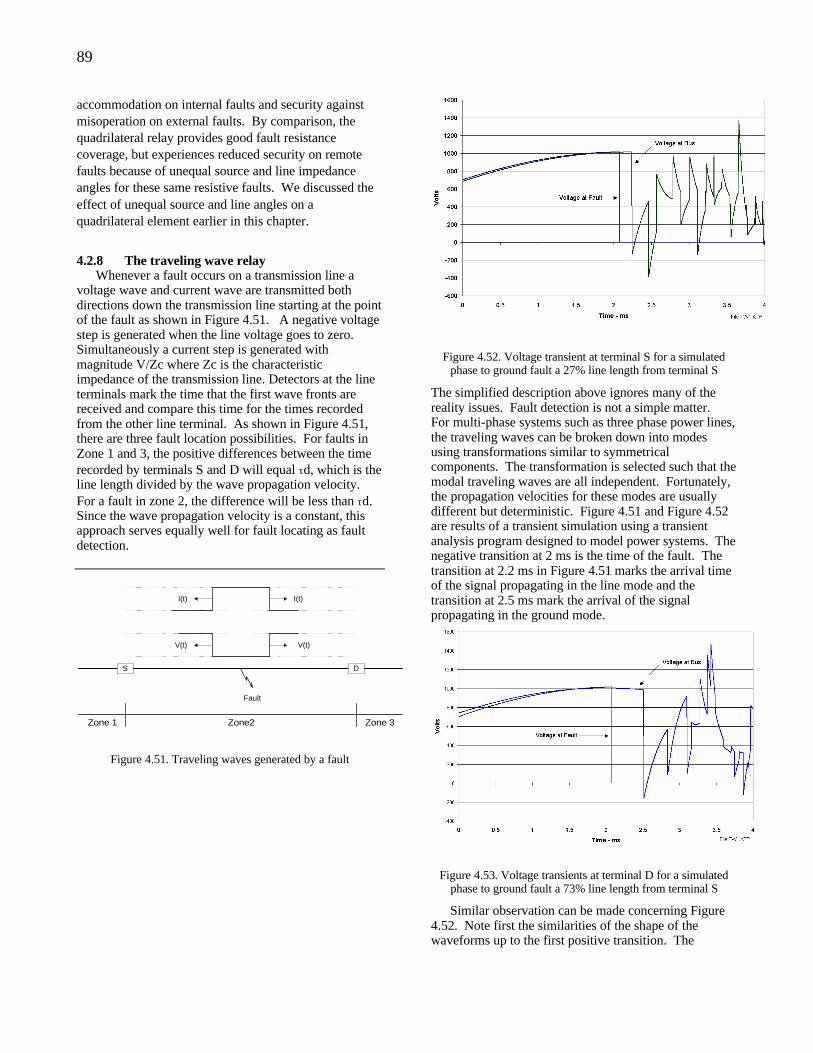
89
accommodation on internal faults and security against misoperation on external faults. By comparison, the quadrilateral relay provides good fault resistance coverage, but experiences reduced security on remote faults because of unequal source and line impedance angles for these same resistive faults. We discussed the effect of unequal source and line angles on a quadrilateral element earlier in this chapter.
4.2.8 The traveling wave relay Whenever a fault occurs on a transmission line a
voltage wave and current wave are transmitted both directions down the transmission line starting at the point of the fault as shown in Figure 4.51. A negative voltage step is generated when the line voltage goes to zero. Simultaneously a current step is generated with magnitude V/Zc where Zc is the characteristic impedance of the transmission line. Detectors at the line terminals mark the time that the first wave fronts are received and compare this time for the times recorded from the other line terminal. As shown in Figure 4.51, there are three fault location possibilities. For faults in Zone 1 and 3, the positive differences between the time recorded by terminals S and D will equal τd, which is the line length divided by the wave propagation velocity. For a fault in zone 2, the difference will be less than τd. Since the wave propagation velocity is a constant, this approach serves equally well for fault locating as fault detection.
I(t)I(t)
V(t) V(t)
Fault
S D
Zone 1 Zone2 Zone 3
Figure 4.51. Traveling waves generated by a fault
Figure 4.52. Voltage transient at terminal S for a simulated phase to ground fault a 27% line length from terminal S
The simplified description above ignores many of the reality issues. Fault detection is not a simple matter. For multi-phase systems such as three phase power lines, the traveling waves can be broken down into modes using transformations similar to symmetrical components. The transformation is selected such that the modal traveling waves are all independent. Fortunately, the propagation velocities for these modes are usually different but deterministic. Figure 4.51 and Figure 4.52 are results of a transient simulation using a transient analysis program designed to model power systems. The negative transition at 2 ms is the time of the fault. The transition at 2.2 ms in Figure 4.51 marks the arrival time of the signal propagating in the line mode and the transition at 2.5 ms mark the arrival of the signal propagating in the ground mode.
Figure 4.53. Voltage transients at terminal D for a simulated phase to ground fault a 73% line length from terminal S
Similar observation can be made concerning Figure 4.52. Note first the similarities of the shape of the waveforms up to the first positive transition. The
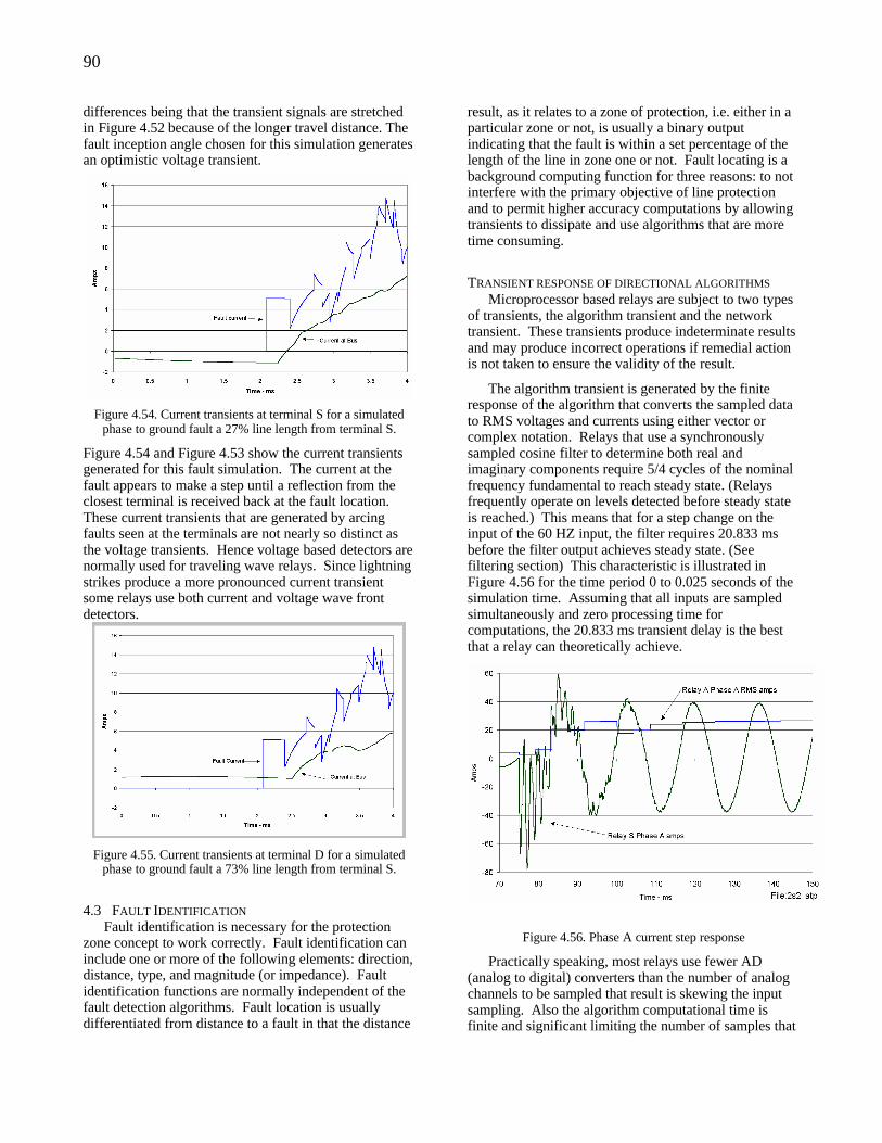
90
differences being that the transient signals are stretched in Figure 4.52 because of the longer travel distance. The fault inception angle chosen for this simulation generates an optimistic voltage transient.
Figure 4.54. Current transients at terminal S for a simulated phase to ground fault a 27% line length from terminal S.
Figure 4.54 and Figure 4.53 show the current transients generated for this fault simulation. The current at the fault appears to make a step until a reflection from the closest terminal is received back at the fault location. These current transients that are generated by arcing faults seen at the terminals are not nearly so distinct as the voltage transients. Hence voltage based detectors are normally used for traveling wave relays. Since lightning strikes produce a more pronounced current transient some relays use both current and voltage wave front detectors.
Figure 4.55. Current transients at terminal D for a simulated phase to ground fault a 73% line length from terminal S.
4.3 FAULT IDENTIFICATION Fault identification is necessary for the protection
zone concept to work correctly. Fault identification can include one or more of the following elements: direction, distance, type, and magnitude (or impedance). Fault identification functions are normally independent of the fault detection algorithms. Fault location is usually differentiated from distance to a fault in that the distance
result, as it relates to a zone of protection, i.e. either in a particular zone or not, is usually a binary output indicating that the fault is within a set percentage of the length of the line in zone one or not. Fault locating is a background computing function for three reasons: to not interfere with the primary objective of line protection and to permit higher accuracy computations by allowing transients to dissipate and use algorithms that are more time consuming.
TRANSIENT RESPONSE OF DIRECTIONAL ALGORITHMS Microprocessor based relays are subject to two types
of transients, the algorithm transient and the network transient. These transients produce indeterminate results and may produce incorrect operations if remedial action is not taken to ensure the validity of the result.
The algorithm transient is generated by the finite response of the algorithm that converts the sampled data to RMS voltages and currents using either vector or complex notation. Relays that use a synchronously sampled cosine filter to determine both real and imaginary components require 5/4 cycles of the nominal frequency fundamental to reach steady state. (Relays frequently operate on levels detected before steady state is reached.) This means that for a step change on the input of the 60 HZ input, the filter requires 20.833 ms before the filter output achieves steady state. (See filtering section) This characteristic is illustrated in Figure 4.56 for the time period 0 to 0.025 seconds of the simulation time. Assuming that all inputs are sampled simultaneously and zero processing time for computations, the 20.833 ms transient delay is the best that a relay can theoretically achieve.
Figure 4.56. Phase A current step response
Practically speaking, most relays use fewer AD (analog to digital) converters than the number of analog channels to be sampled that result is skewing the input sampling. Also the algorithm computational time is finite and significant limiting the number of samples that
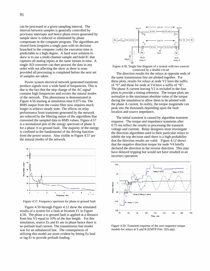
91
can be processed in a given sampling interval. The interval between samples is generally controlled by processor interrupts and hence phase errors generated by sample skew is reduced or eliminated by phase compensate in the computer program. The algorithms are closed form (requires a single pass with no decision branched in the computer code) the execution time is predictable to a high degree. A hard ware solution to skew is to use a multi-channel sample and hold IC that captures all analog inputs at the same instant in time. A single AD converter can then process the data in any order with out affecting the skew as there is none provided all processing is completed before the next set of samples are taken.
Power system electrical network generated transients produce signals over a wide band of frequencies. This is due to the fact that the step change of the AC signal contains high frequencies and excites the natural modes of the network. This phenomena is demonstrated in Figure 4.56 starting at simulation time 0.075 ms. The RMS output from the cosine filter now requires much longer is achieve steady state. The effects on relay performance from transients generated by the network are reduced by the filtering nature of the algorithms that converted the sampled data to RMS values. Figure 4.57 is a normalized plot of the energy spectrum of phase A for a phase A to ground fault. The majority of the energy is confined to the fundamental of the driving function from the power source. Also visible in Figure 4.57 are the natural modes of the network.
Figure 4.57. Frequency spectrum for phase to ground fault
Figure 4.59 through Figure 4.12 show the simulated results of a system for a fault at location F1 in Figure 4.58. The phase a to ground fault is applied at a distance from bus V2 equal to 10% of the line length. For this simulation, source Es and Er are in phase hence there is no prefault load current. The transmission line model was for an unbalanced line. The consequences of utilizing this model are more evident by letting Es lead or lag Er to provide prefault loading.
Rr
Vr,IrRelay R
Rs
Vs,IsRelay S
ZL*m2 ZL*(1-m2)
ZL*m1 ZL*(1-m1)
Fault
Line #1
Line #2
Zt
ISpol
Es ZL*m3ZSRC
Bus S
ErZrr
Bus R
IrIs
IsREV IsFOR
Figure 4.58. Single line diagram of a system with two sources connected by a double circuit
The direction results for the relays at opposite ends of the same transmission line are plotted together. For these plots, results for relays at node V2 have the suffix of “S” and those for node at V4 have a suffix of “R”. The phase A current leaving V2 is included in the four plots to provide a timing reference. The torque plots are normalize to the maximum absolute value of the torque during the simulation to allow them to be plotted with the phase A current. In reality, the torque magnitude can peak into the thousands depending upon the fault location and source impedance.
The initial transient is caused by algorithm transient response. The torque and impedance transients after 0.75 ms reflect the results in processing the transient voltage and currents. Relay designers must investigate the direction algorithms used in their particular relays to inhibit the trip decision until there is a high probability that the direction results are valid. Figure 4.12 shows that the negative direction torque for node V4 briefly declared the direction in the reverse direction. This may have delayed tripping but would not have resulted in an incorrect operation.
Figure 4.59. Transient response of the zero sequence torque models for relays at S and R (EMTP File: 2l2s.atp).
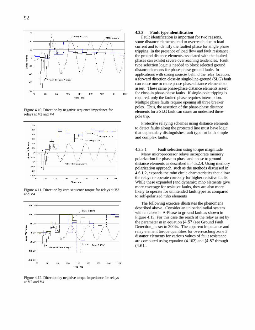
92
Figure 4.10. Direction by negative sequence impedance for relays at V2 and V4
Figure 4.11. Direction by zero sequence torque for relays at V2 and V4
Figure 4.12. Direction by negative torque impedance for relays at V2 and V4
4.3.3 Fault type identification Fault identification is important for two reasons,
some distance elements tend to overreach due to load current and to identify the faulted phase for single phase tripping. In the presence of load flow and fault resistance, the ground distance elements associated with the faulted phases can exhibit severe overreaching tendencies. Fault type selection logic is needed to block selected ground distance elements for phase-phase-ground faults. In applications with strong sources behind the relay location, a forward direction close-in single-line-ground (SLG) fault can cause one or more phase-phase distance elements to assert. These same phase-phase distance elements assert for close-in phase-phase faults. If single-pole tripping is required, only the faulted phase requires interruption. Multiple phase faults require opening all three breaker poles. Thus, the assertion of the phase-phase distance elements for a SLG fault can cause an undesired three-pole trip.
Protective relaying schemes using distance elements to detect faults along the protected line must have logic that dependably distinguishes fault type for both simple and complex faults.
4.3.3.1 Fault selection using torque magnitude Many microprocessor relays incorporate memory
polarization for phase to phase and phase to ground distance elements as described in 4.5.2.4. Using memory polarization approach, such as the methods discussed in 4.6.1.2, expands the mho circle characteristics that allow the relays to operate correctly for higher resistive faults. While these expanded (and dynamic) mho elements give more coverage for resistive faults, they are also more likely to operate for unintended fault types as compared to self-polarized mho elements
The following exercise illustrates the phenomena described above. Consider an unloaded radial system with an close in A-Phase to ground fault as shown in Figure 4.13. For this case the reach of the relay as set by the parameter m in equation (4.57 (see Ground Fault Detection_ is set to 300%. The apparent impedance and relay element torque quantities for overreaching zone 3 distance elements for various values of fault resistance are computed using equation (4.102) and (4.57 through (4.61..
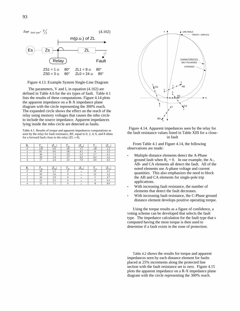
93
IVZapt typefault = (4.102)
Relay
Zs ZL
Fault
Es
m(p.u.) of ZL
ZS1 = 1 Ω ∠ 80°ZS0 = 3 Ω ∠ 80°
ZL1 = 8 Ω ∠ 80°ZL0 = 24 Ω ∠ 80°
Figure 4.13. Example System Single-Line Diagram
The parameters, V and I, in equation (4.102) are defined in Table 4.6 for the six types of fault. Table 4.1 lists the results of these computations. Figure 4.14 plots the apparent impedance on a R-X impedance plane diagram with the circle representing the 300% reach. The expanded circle shows the effect on the reach of the relay using memory voltages that causes the mho circle to include the source impedance. Apparent impedances lying inside the mho circle are detected as faults.
Table 4.1. Results of torque and apparent impedances computations as seen by the relay for fault resistance, RF, equal to 0, 2, 4, 6, and 8 ohms for a forward fault close to the relay (ZL » 0).
RF TAG |ZAG| TBG |ZBG| TCG |ZCG| 0 118 0.0 -30 3.1 -29 3.1 1 81 0.6 -38 4.1 -6 3.3 2 46 1.2 -33 5.2 2.7 4.1 3 28 1.8 -27 6.5 4.2 5.2 4 17 2.4 -23 7.9 4.0 6.5
RF TAB |ZAB| TBC |ZBC| TCA |ZCA| 0 56 2.1 0 ∞ 55 2.1 1 50 2.6 0 ∞ 22 3.2 2 34 3.9 0 ∞ 3 4.7 3 22 5.5 0 ∞ -5 6.3 4 15 7.1 0 ∞ -8 8.0
AG
BG
CG AB
CA
2
4
0
0
4
0
40
4
R
X LINE ANGLE
SELF-POLARIZED
EXPANDED
CHARACTERISTICS
REACH = Z00%•Z1L
Figure 4.14. Apparent impedances seen by the relay for the fault resistance values listed in Table XIII for a close-
in fault
From Table 4.1 and Figure 4.14, the following observations are made:
• Multiple distance elements detect the A-Phase ground fault when RF = 0. In our example, the A-, AB- and CA elements all detect the fault. All of the noted elements use A-phase voltage and current quantities. This also emphasizes the need to block the AB and CA elements for single-pole trip applications.
• With increasing fault resistance, the number of elements that detect the fault decreases.
• With increasing fault resistance, the C-Phase ground distance element develops positive operating torque.
Using the torque results as a figure of confidence, a
voting scheme can be developed that selects the fault type. The impedance calculation for the fault type that s computed having the most torque is then used to determine if a fault exists in the zone of protection.
Table 4.2 shows the results for torque and apparent impedances seen by each distance element for faults placed at 25% increments along the protected line section with the fault resistance set to zero. Figure 4.15 plots the apparent impedance on a R-X impedance plane diagram with the circle representing the 300% reach.
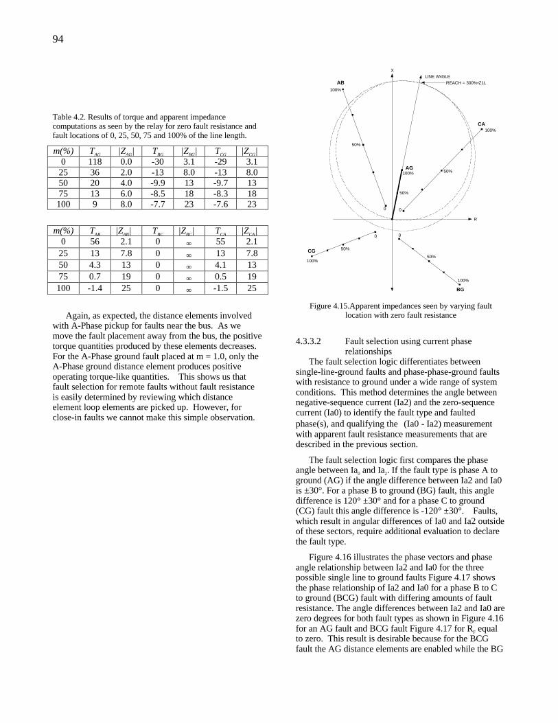
94
Table 4.2. Results of torque and apparent impedance computations as seen by the relay for zero fault resistance and fault locations of 0, 25, 50, 75 and 100% of the line length.
m(%) TAG |ZAG| TBG |ZBG| TCG |ZCG| 0 118 0.0 -30 3.1 -29 3.1
25 36 2.0 -13 8.0 -13 8.0 50 20 4.0 -9.9 13 -9.7 13 75 13 6.0 -8.5 18 -8.3 18 100 9 8.0 -7.7 23 -7.6 23
m(%) TAB |ZAB| TBC |ZBC| TCA |ZCA| 0 56 2.1 0 ∞ 55 2.1
25 13 7.8 0 ∞ 13 7.8 50 4.3 13 0 ∞ 4.1 13 75 0.7 19 0 ∞ 0.5 19 100 -1.4 25 0 ∞ -1.5 25
Again, as expected, the distance elements involved with A-Phase pickup for faults near the bus. As we move the fault placement away from the bus, the positive torque quantities produced by these elements decreases. For the A-Phase ground fault placed at m = 1.0, only the A-Phase ground distance element produces positive operating torque-like quantities. This shows us that fault selection for remote faults without fault resistance is easily determined by reviewing which distance element loop elements are picked up. However, for close-in faults we cannot make this simple observation.
AG
BG
CG
AB
CA
0
0
0
0
R
XLINE ANGLE
REACH = 300%•Z1L
100%
50%
50%
100%
50%
100%
50%
100%
100%
50%
Figure 4.15.Apparent impedances seen by varying fault
location with zero fault resistance
4.3.3.2 Fault selection using current phase relationships
The fault selection logic differentiates between single-line-ground faults and phase-phase-ground faults with resistance to ground under a wide range of system conditions. This method determines the angle between negative-sequence current (Ia2) and the zero-sequence current (Ia0) to identify the fault type and faulted phase(s), and qualifying the∠(Ia0 - Ia2) measurement with apparent fault resistance measurements that are described in the previous section.
The fault selection logic first compares the phase angle between Ia0 and Ia2. If the fault type is phase A to ground (AG) if the angle difference between Ia2 and Ia0 is ±30°. For a phase B to ground (BG) fault, this angle difference is 120° ±30° and for a phase C to ground (CG) fault this angle difference is -120° ±30°. Faults, which result in angular differences of Ia0 and Ia2 outside of these sectors, require additional evaluation to declare the fault type.
Figure 4.16 illustrates the phase vectors and phase angle relationship between Ia2 and Ia0 for the three possible single line to ground faults Figure 4.17 shows the phase relationship of Ia2 and Ia0 for a phase B to C to ground (BCG) fault with differing amounts of fault resistance. The angle differences between Ia2 and Ia0 are zero degrees for both fault types as shown in Figure 4.16 for an AG fault and BCG fault Figure 4.17 for RF equal to zero. This result is desirable because for the BCG fault the AG distance elements are enabled while the BG
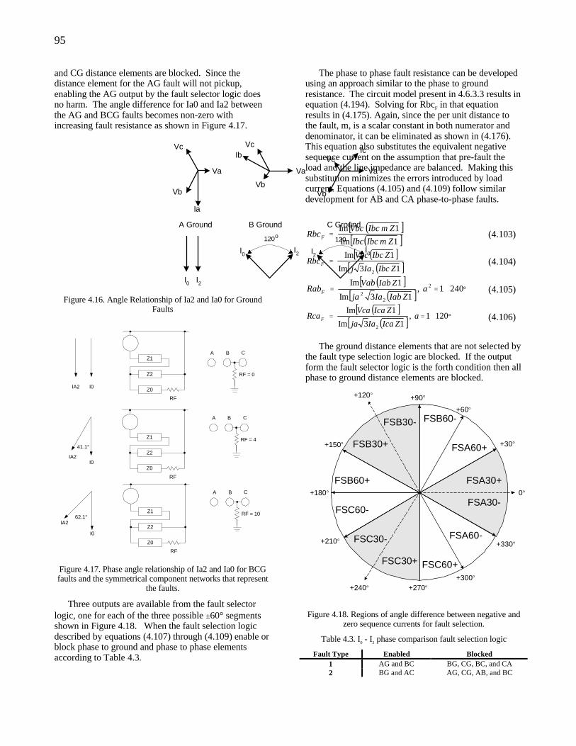
95
and CG distance elements are blocked. Since the distance element for the AG fault will not pickup, enabling the AG output by the fault selector logic does no harm. The angle difference for Ia0 and Ia2 between the AG and BCG faults becomes non-zero with increasing fault resistance as shown in Figure 4.17.
Va
Vb
Vc
Ia
Va
Vb
VcIb
Va
Vb
VcIc
A Ground B Ground C Ground
I0 I2
120o120
I0 I0I2 I2
Figure 4.16. Angle Relationship of Ia2 and Ia0 for Ground
Faults
Z1
Z2
Z0
RF
IA2
I0
A B C
RF = 1062.1°
Z1
Z2
Z0
RF
IA2I0
A B C
RF = 441.1°
Z1
Z2
Z0
RF
A B C
IA2 I0
RF = 0
Figure 4.17. Phase angle relationship of Ia2 and Ia0 for BCG faults and the symmetrical component networks that represent
the faults.
Three outputs are available from the fault selector logic, one for each of the three possible ±60° segments shown in Figure 4.18. When the fault selection logic described by equations (4.107) through (4.109) enable or block phase to ground and phase to phase elements according to Table 4.3.
The phase to phase fault resistance can be developed using an approach similar to the phase to ground resistance. The circuit model present in 4.6.3.3 results in equation (4.194). Solving for RbcF in that equation results in (4.175). Again, since the per unit distance to the fault, m, is a scalar constant in both numerator and denominator, it can be eliminated as shown in (4.176). This equation also substitutes the equivalent negative sequence current on the assumption that pre-fault the load and the line impedance are balanced. Making this substitution minimizes the errors introduced by load current. Equations (4.105) and (4.109) follow similar development for AB and CA phase-to-phase faults.
( )[ ]( )[ ]1Im
1Im
ZmIbcIbc
ZmIbcVbcRbcF =
(4.103)
( )[ ]( )[ ]13Im
1Im
2 ZIbcIaj
ZIbcVbcRbcF = (4.104)
( )[ ]( )[ ] °∠== 2401,
13Im
1Im 2
22
aZIabIaja
ZIabVabRabF
(4.105)
( )[ ]( )[ ]
°∠== 1201,13Im
1Im
2
aZIcaIaja
ZIcaVcaRcaF
(4.106)
The ground distance elements that are not selected by
the fault type selection logic are blocked. If the output form the fault selector logic is the forth condition then all phase to ground distance elements are blocked.
17 %
17 %
9 %
8 %
16 %
17 %
16 %
FSA30+
+30°
+60°
+90°
+150°
+180°
+210°
+270°
+300°
+330°
+120°
+240°
0°
FSA30-
FSC30+
FSB30+
FSC30-
FSB30-
FSA60+
FSA60-
FSC60+
FSB60+
FSB60-
FSC60-
Figure 4.18. Regions of angle difference between negative and zero sequence currents for fault selection.
Table 4.3. I0 - I2 phase comparison fault selection logic
Fault Type Enabled Blocked 1 AG and BC BG, CG, BC, and CA 2 BG and AC AG, CG, AB, and BC
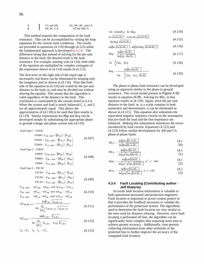
96
3 CG and AB AG, BG, BC, and CA 4 AB, BC, CA All but ABC-G
This method requires the computation of the fault
resistance. This can be accomplished by writing the loop equations for the various fault conditions. The results are provided in equations (4.119) through (4.123) while the fundamental approach is developed in 4.1.9 . The difference being that instead of solving for the per-unit distance to the fault, the desired result is the fault resistance. For example, starting with (4.124), both sides of the equation are multiplied by complex conjugate of the expression shown in (4.114) results in (4.115).
The first term on the right side of the equal sign is necessarily real hence can be eliminated by keeping only the imaginary part as shown in (4.116). Note that both side of the equation in (4.116) are scaled by the per-unit distance to the fault, m, and may be divided out without altering the equality. This means that the algorithm is valid regardless of the distance to the fault. This conclusion is constrained by the caveats listed in 4.3.4. When the system and load is nearly balanced I1, I2. and I0 are all approximately equal. This allows the approximation of (4.118) to be used that then results in (4.119). Similar expressions for Rbg and Rcg can be developed simply by substituting the appropriate phase to ground voltage and phase current into (4.119).
( )( )( )ACAGMINCA
BCAGMINBC
ABAGMINAB
RRZFSA
RRZFSA
RRZFSA
FSATypeFault
<••+
<••+
<••+
=
−
−
−
60
60
60
301
(4.107)
( )( )( )ACBGMINCA
BCBGMINBC
ABBGMINAB
RRZFSB
RRZFSB
RRZFSB
FSBTypeFault
<••+
<••+
<••+
=
−
−
−
60
60
60
302
(4.108)
( )( )( )ACCGMINCA
BCCGMINBC
ABCGMINAB
RRZFSC
RRZFSC
RRZFSC
FSCTypeFault
<••+
<••+
<••+
=
−
−
−
60
60
60
303
(4.109)
CAABBCABMINAB ZmZmandmZmZZ <<⇒−
CABCABBCMINBC mZmZandmZmZZ <<⇒−
ABCABCCAMINCA mZZmandmZmZZ <<⇒− (4.110)
( )
⋅
⋅=
CABCABCABCAB
CABCABABCABCAB
IIZL
ZL
IVmZ
,,,,1
1
,,,,
Im
Im
(4.111)
( )( )( )( )
+⋅
⋅=
CBARCBA
CBACBACBA
IIkIZL
ZL
IVmZ
,,0.,1
1
,,,,,,
Im
Im,
(4.112)
( ) oCBAR IIIII 3=++= (4.113)
RagIamZLIaVa ⋅+= )( 1 (4.114)
( ) ( )
( )( ))(
)()()(
1
111
ZLIamRagIa
ZLIamZLIamZLIamVa += (4.115)
( )[ ] ( )( )[ ])(Im)(Im 11 ZLIamRagIaZLIamVa = (4.116)
( )[ ]( )( )[ ]1
1
Im
Im
ZLIaIa
ZLIaVaRag = (4.117)
)(2
320 IaIaIa +≅ (4.118)
( )[ ]( )
+
=
120
1
)(2
3Im
Im
ZLIaIaIa
ZLIaVaRag
(4.119)
The phase to phase fault resistance can be developed
using an approach similar to the phase to ground resistance. The circuit model present in Figure 4.50 results in equation (4.95. Solving for RbcF in that equation results in (4.120). Again, since the per unit distance to the fault, m, is a scalar constant in both numerator and denominator, it can be eliminated as shown in (4.121). This equation also substitutes the equivalent negative sequence current on the assumption that pre-fault the load and the line impedance are balanced. Making this substitution minimizes the errors introduced by load current. Equations (4.122) and (4.123) follow similar development for AB and CA phase to phase faults.
( )[ ]( )[ ]1
1
Im
Im
ZLmIbcIbc
ZLmIbcVbcRbcF = (4.1
20)
( )[ ]( )[ ]12
1
3Im
Im
ZLIbcIaj
ZLIbcVbcRbcF = (4.1
21)
( )[ ]( )[ ] °∠== 2401,
3Im
Im 2
122
1 aZLIabIaja
ZLIabVabRabF (4.1
22)
( )[ ]( )[ ] °∠== 1201,
3Im
Im
12
1 aZLIcaIaja
ZLIcaVcaRcaF (4.1
23)
4.3.4 Fault Locating (Contributing author - Jeff Roberts)
Accurate fault location information is valuable to both operational personnel and protection engineers. Fault location is important to power system protect in that it provides the feedback necessary to validate the performance of the protection system. The algorithms used to determine the fault location are very similar to the ones used for distance relaying. However, since fault locating is performed off line, the algorithm can be significantly more complex thus requiring more time to achieve greater accuracy. Additionally, time permits collecting information from other terminals of the protected line to further improve the accuracy of the computed fault location.
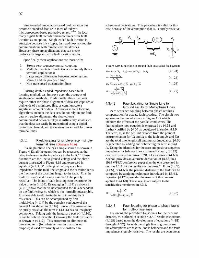
97
Single-ended, impedance-based fault location has become a standard feature in most of today’s microprocessor-based protective relays.xvi,xvii In fact, many digital fault recorder manufacturers offer fault location as an option. Single-ended fault location is attractive because it is simple, fast, and does not require communications with remote terminal devices. However, there are applications that can create undesirably large errors in fault location results.
Specifically these applications are those with:
1. Strong zero-sequence mutual coupling 2. Multiple remote terminals (most commonly three-
terminal applications) 3. Large angle differences between power system
sources and the protected line 4. Non-transposed transmission lines
Existing double-ended impedance-based fault
locating methods can improve upon the accuracy of single-ended methods. Traditionally, these methods require either the phase alignment of data sets captured at both ends of a monitored line, or communicate a significant amount of data. Advances in fault locating algorithms include: the data sets do not rely on pre-fault data or require alignment, the data volume communicated between relays is sufficiently small such that the data can easily be transmitted using a digital protection channel, and the system works well for three-terminal lines.
4.3.4.1 Fault locating for single-phase – single-terminal lines (Distance Mho)
If a single-phase line has a single source as shown in Figure 4.13, all the quantities can be measured at the relay to determine the impedance to the fault.xviii These quantities are the line to ground voltage and the phase current illustrated in Figure 4.19 and expressed in equation (4.114). ZL is the positive sequence line impedance for the total line length and the m multiplier is the fraction of the total line length to the fault. RF is the fault resistance and usually assumed to be purely resistive. The focus of fault locating is to determine the value of m in (4.114). Rearranging (4.114) as shown in (4.115) show that the value computed for m is dependent on the fault resistance which is not normally measurable. It is desirable to eliminate the term involving fault resistance. This can be accomplished by first multiplying (4.114) by the complex conjugate of the current Ia as shown in (4.116). Since RF is assumed to be purely resistive, the term in (4.116) has no imaginary component. Taking only the imaginary part of (4.116), m can be solved for without knowing the fault resistance as shown in (4.117). This procedure to eliminate an unwanted term (for whatever reason that suits our purpose) is used extensively as demonstrated in
subsequent derivations. This procedure is valid for this case because of the assumption that RF is purely resistive.
EA
mZL
RF
IAVAZS VF
IF
Figure 4.19. Single line to ground fault on a radial feed system
FLFL RIaZIamRmZIaVa +=+= )1()1( (4.124)
L
F
ZIa
RIaVam
1
−= (4.125)
( )IaRIaIaZIamIaVa FL += )1( (4.126)
[ ][ ]IaZIa
IaVam
L )1(Im
Im= (4.127)
4.3.4.2 Fault Locating for Single Line to Ground Faults for Multi-phase Lines
Zero sequence coupling between phases requires compensation for actuate fault locating. The circuit now appears as the model shown in Figure 4.22 which includes the effects of the parallel conductors. The faulted phase loop equation is expressed by (4.63 and further clarified by (4.64 as developed in section 4.1.9. The term, m, is the per unit distance from the point of instrumentation for Va and Ia to the fault and Zs and Zm are the total line length self and mutual impedance. (4.65 is generated by adding and subtracting the term m(Zm) Ia. Using the identities for the zero and positive sequence impedance for balance lines expressed by and , (4.113) can be expressed in terms of Z0, Z1 as shown in (4.68). Zocholl provides an alternate derivation of (4.68) in a 1995 WPRC conference paper than the one presented in section 4.1.9 but the results are the same.xix From (4.63), (4.65), or (4.68), the per-unit distance to the fault can be computed by applying techniques introduced in 4.3.4.1. Equation (4.128) provides the results of this process applied to (4.68). These results are subject to the sensitivities mentioned in 4.3.4.
( )( )( )IaIakIaZL
aIVam
001Im
Im
−= (4.128)
4.3.4.3 Fault locating for phase to phase faults for multi-phase lines
Following the procedure for solving for the per-unit distance, m, outlined in section 4.3.4.1 results in equation (4.129) based upon the development of equations (4.88) through (4.92). As with the single line to ground case, the assumptions are that the line is balanced and the fault impedance is purely resistive. The results are accurate as
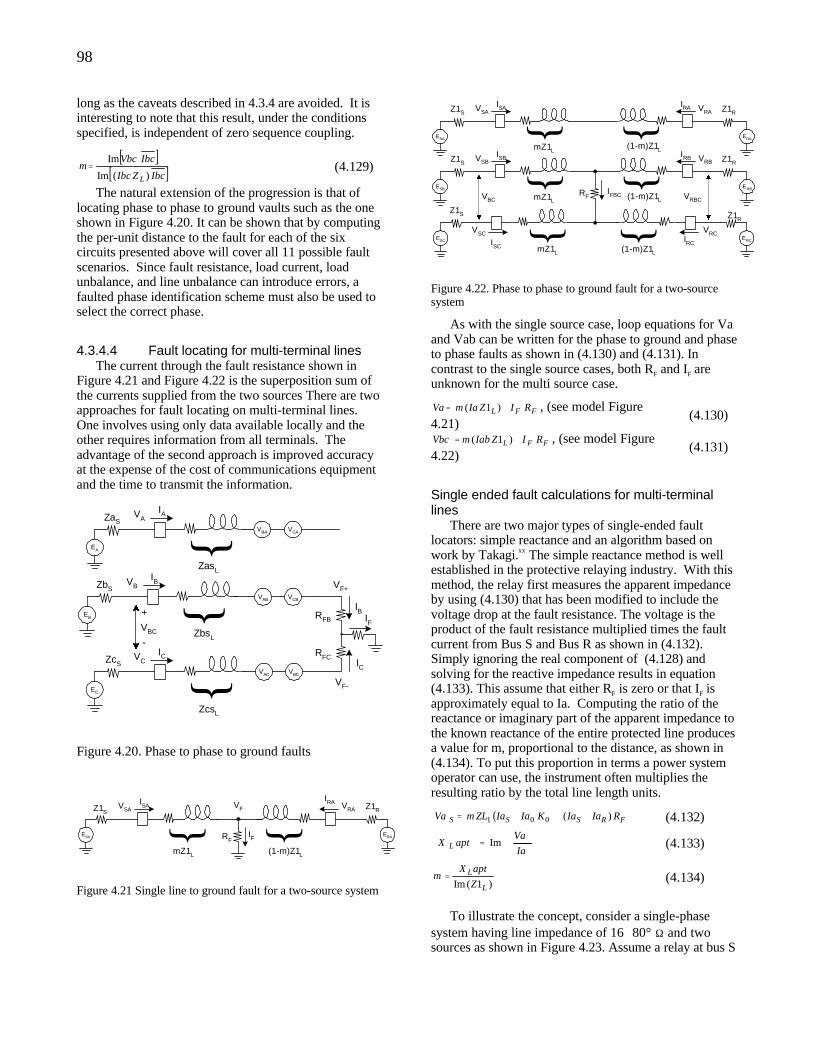
98
long as the caveats described in 4.3.4 are avoided. It is interesting to note that this result, under the conditions specified, is independent of zero sequence coupling.
[ ][ ]IbcZIbc
IbcVbcm
L )(Im
Im= (4.129)
The natural extension of the progression is that of locating phase to phase to ground vaults such as the one shown in Figure 4.20. It can be shown that by computing the per-unit distance to the fault for each of the six circuits presented above will cover all 11 possible fault scenarios. Since fault resistance, load current, load unbalance, and line unbalance can introduce errors, a faulted phase identification scheme must also be used to select the correct phase.
4.3.4.4 Fault locating for multi-terminal lines The current through the fault resistance shown in
Figure 4.21 and Figure 4.22 is the superposition sum of the currents supplied from the two sources There are two approaches for fault locating on multi-terminal lines. One involves using only data available locally and the other requires information from all terminals. The advantage of the second approach is improved accuracy at the expense of the cost of communications equipment and the time to transmit the information.
RFB
VF+
IB
EA
ZasL
IAVAZaS
EB
ZbsL
IBVBZbS
EC
ZcsL
ICVCZcS
VBA
VAB
VAC
VCA
VCB
VBC
VF-
VBC
+
-
ICRFC
IF
Figure 4.20. Phase to phase to ground faults
RF
VF
IF ERA
(1-m)Z1L
VRA
ESA
mZ1L
ISAVSAZ1S
IRAZ1R
Figure 4.21 Single line to ground fault for a two-source system
ESB
RF
ISBVSBZ1S
IFBC
ESC
VSC
VBC
ERB
IRB VRB
ERC
Z1R
VRCIRC
VRBC
mZ1L
ISC (1-m)Z1L
mZ1L(1-m)Z1L
Z1S
Z1R
ESA
ISAVSAZ1S
ERA
IRA VRA
mZ1L(1-m)Z1L
Z1R
Figure 4.22. Phase to phase to ground fault for a two-source system
As with the single source case, loop equations for Va and Vab can be written for the phase to ground and phase to phase faults as shown in (4.130) and (4.131). In contrast to the single source cases, both RF and IF are unknown for the multi source case.
FFL RIZIamVa += )1( , (see model Figure 4.21)
(4.130)
FFL RIZIabmVbc += )1( , (see model Figure 4.22)
(4.131)
Single ended fault calculations for multi-terminal lines
There are two major types of single-ended fault locators: simple reactance and an algorithm based on work by Takagi.xx The simple reactance method is well established in the protective relaying industry. With this method, the relay first measures the apparent impedance by using (4.130) that has been modified to include the voltage drop at the fault resistance. The voltage is the product of the fault resistance multiplied times the fault current from Bus S and Bus R as shown in (4.132). Simply ignoring the real component of (4.128) and solving for the reactive impedance results in equation (4.133). This assume that either RF is zero or that IF is approximately equal to Ia. Computing the ratio of the reactance or imaginary part of the apparent impedance to the known reactance of the entire protected line produces a value for m, proportional to the distance, as shown in (4.134). To put this proportion in terms a power system operator can use, the instrument often multiplies the resulting ratio by the total line length units.
( ) FRSSS RIaIaKIaIaZLmVa )(001 +++= (4.132)
=
Ia
VaaptX L Im (4.133)
)1(Im L
L
Z
aptXm = (4.134)
To illustrate the concept, consider a single-phase
system having line impedance of 16∠80° Ω and two sources as shown in Figure 4.23. Assume a relay at bus S
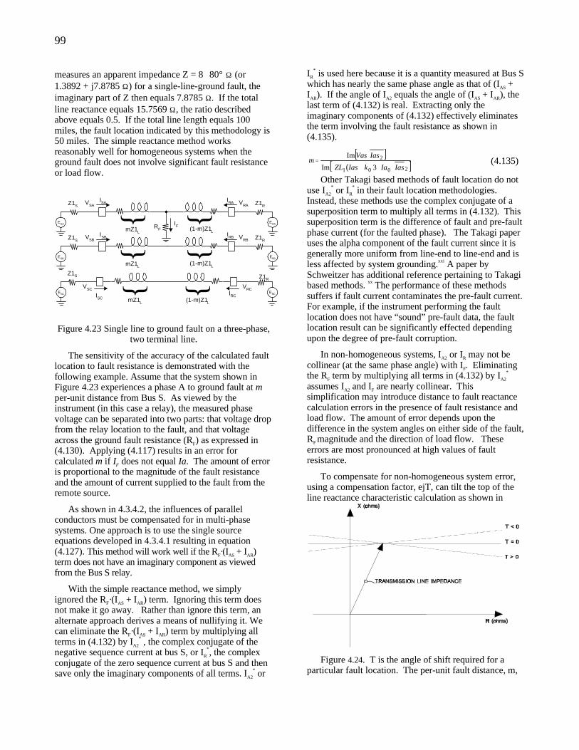
99
measures an apparent impedance Z = 8∠80° Ω (or 1.3892 + j7.8785 Ω) for a single-line-ground fault, the imaginary part of Z then equals 7.8785 Ω. If the total line reactance equals 15.7569 Ω, the ratio described above equals 0.5. If the total line length equals 100 miles, the fault location indicated by this methodology is 50 miles. The simple reactance method works reasonably well for homogeneous systems when the ground fault does not involve significant fault resistance or load flow.
ESB
RF
ISBVSBZ1S
ESC
VSC
ERB
IRB VRB
ERC
Z1R
VRCIRC
mZ1L
ISC (1-m)Z1L
mZ1L(1-m)Z1L
Z1S
Z1R
ESA
ISAVSAZ1S
ERA
IRA VRA
mZ1L(1-m)Z1L
Z1R
IF
Figure 4.23 Single line to ground fault on a three-phase, two terminal line.
The sensitivity of the accuracy of the calculated fault location to fault resistance is demonstrated with the following example. Assume that the system shown in Figure 4.23 experiences a phase A to ground fault at m per-unit distance from Bus S. As viewed by the instrument (in this case a relay), the measured phase voltage can be separated into two parts: that voltage drop from the relay location to the fault, and that voltage across the ground fault resistance (RF) as expressed in (4.130). Applying (4.117) results in an error for calculated m if IF does not equal Ia. The amount of error is proportional to the magnitude of the fault resistance and the amount of current supplied to the fault from the remote source.
As shown in 4.3.4.2, the influences of parallel conductors must be compensated for in multi-phase systems. One approach is to use the single source equations developed in 4.3.4.1 resulting in equation (4.127). This method will work well if the RF·(IAS + IAR) term does not have an imaginary component as viewed from the Bus S relay.
With the simple reactance method, we simply ignored the RF·(IAS + IAR) term. Ignoring this term does not make it go away. Rather than ignore this term, an alternate approach derives a means of nullifying it. We can eliminate the RF·(IAS + IAR) term by multiplying all terms in (4.132) by IA2
* , the complex conjugate of the negative sequence current at bus S, or IR
*, the complex conjugate of the zero sequence current at bus S and then save only the imaginary components of all terms. IA2
* or
IR
* is used here because it is a quantity measured at Bus S which has nearly the same phase angle as that of (IAS + IAR). If the angle of IA2 equals the angle of (IAS + IAR), the last term of (4.132) is real. Extracting only the imaginary components of (4.132) effectively eliminates the term involving the fault resistance as shown in (4.135).
[ ]( )[ ]2001
2
3Im
Im
IasIakIasZL
IasVasm
⋅+= (4.135)
Other Takagi based methods of fault location do not use IA2
* or IR
* in their fault location methodologies. Instead, these methods use the complex conjugate of a superposition term to multiply all terms in (4.132). This superposition term is the difference of fault and pre-fault phase current (for the faulted phase). The Takagi paper uses the alpha component of the fault current since it is generally more uniform from line-end to line-end and is less affected by system grounding.xxi A paper by Schweitzer has additional reference pertaining to Takagi based methods. xx The performance of these methods suffers if fault current contaminates the pre-fault current. For example, if the instrument performing the fault location does not have “sound” pre-fault data, the fault location result can be significantly effected depending upon the degree of pre-fault corruption.
In non-homogeneous systems, IA2 or IR may not be collinear (at the same phase angle) with IF. Eliminating the RF term by multiplying all terms in (4.132) by IA2
* assumes IA2 and IF are nearly collinear. This simplification may introduce distance to fault reactance calculation errors in the presence of fault resistance and load flow. The amount of error depends upon the difference in the system angles on either side of the fault, RF magnitude and the direction of load flow. These errors are most pronounced at high values of fault resistance.
To compensate for non-homogeneous system error, using a compensation factor, ejT, can tilt the top of the line reactance characteristic calculation as shown in
Figure 4.24. T is the angle of shift required for a particular fault location. The per-unit fault distance, m,
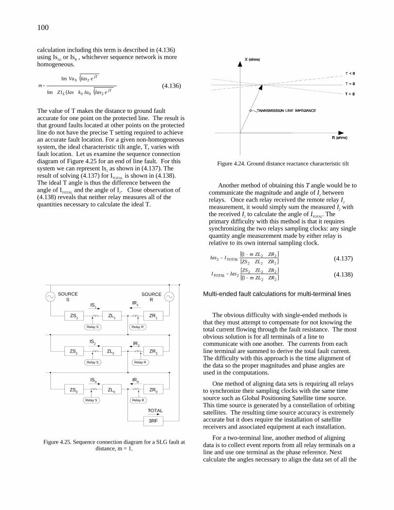
100
calculation including this term is described in (4.136) using IsA2 or IsR , whichever sequence network is more homogeneous.
( )
( )( )
+
=jT
L
jTS
eIasIakIasZ
eIasVam
200
2
1Im
Im (4.136)
The value of T makes the distance to ground fault accurate for one point on the protected line. The result is that ground faults located at other points on the protected line do not have the precise T setting required to achieve an accurate fault location. For a given non-homogeneous system, the ideal characteristic tilt angle, T, varies with fault location. Let us examine the sequence connection diagram of Figure 4.25 for an end of line fault. For this system we can represent Is2 as shown in (4.137). The result of solving (4.137) for ITOTAL is shown in (4.138). The ideal T angle is thus the difference between the angle of ITOTAL and the angle of I2. Close observation of (4.138) reveals that neither relay measures all of the quantities necessary to calculate the ideal T.
Figure 4.24. Ground distance reactance characteristic tilt
Another method of obtaining this T angle would be to communicate the magnitude and angle of I2 between relays. Once each relay received the remote relay I2 measurement, it would simply sum the measured I2 with the received I2 to calculate the angle of ITOTAL. The primary difficulty with this method is that it requires synchronizing the two relays sampling clocks: any single quantity angle measurement made by either relay is relative to its own internal sampling clock.
( )[ ][ ]222
222
1
ZRZLZS
ZRZLmIIas TOTAL
++
+−= (4.137)
[ ]( )[ ]22
2222 1 ZRZLm
ZRZLZSIasITOTAL
+−
++= (4.138)
ZL1ZS1 ZR1
3RF
SOURCES
SOURCER
ITOTAL
ZS2
ZS0
ZL2
ZR0
ZR2
ZL0
IS0
IS2
IS1IR1
IR2
IR0
Relay S
Relay S
Relay S Relay R
Relay R
Relay R
Figure 4.25. Sequence connection diagram for a SLG fault at distance, m = 1.
Multi-ended fault calculations for multi-terminal lines
The obvious difficulty with single-ended methods is
that they must attempt to compensate for not knowing the total current flowing through the fault resistance. The most obvious solution is for all terminals of a line to communicate with one another. The currents from each line terminal are summed to derive the total fault current. The difficulty with this approach is the time alignment of the data so the proper magnitudes and phase angles are used in the computations.
One method of aligning data sets is requiring all relays to synchronize their sampling clocks with the same time source such as Global Positioning Satellite time source. This time source is generated by a constellation of orbiting satellites. The resulting time source accuracy is extremely accurate but it does require the installation of satellite receivers and associated equipment at each installation.
For a two-terminal line, another method of aligning data is to collect event reports from all relay terminals on a line and use one terminal as the phase reference. Next calculate the angles necessary to align the data set of all the
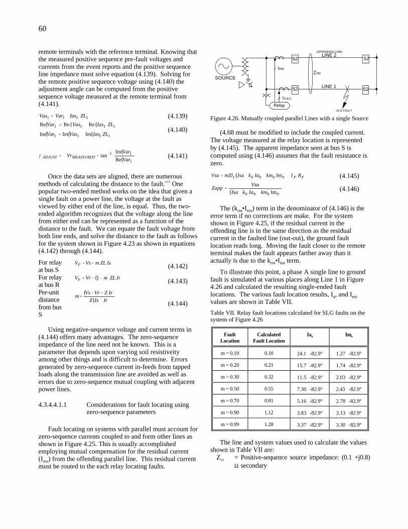
60
remote terminals with the reference terminal. Knowing that the measured positive sequence pre-fault voltages and currents from the event reports and the positive sequence line impedance must solve equation (4.139). Solving for the remote positive sequence voltage using (4.140) the adjustment angle can be computed from the positive sequence voltage measured at the remote terminal from (4.141).
1111 ZLIasVarVas += (4.139) ( ) ( ) ( )
( ) ( ) ( )1111
1111
ImImIm
ReReRe
ZLIasVasVar
ZLIasVasVar
+=
+= (4.140)
( )( )
−∠= −
1
11
Re
Imtan
Var
VarVrMEASYUREDADJUSTφ (4.141)
Once the data sets are aligned, there are numerous
methods of calculating the distance to the fault.xxii One popular two-ended method works on the idea that given a single fault on a power line, the voltage at the fault as viewed by either end of the line, is equal. Thus, the two-ended algorithm recognizes that the voltage along the line from either end can be represented as a function of the distance to the fault. We can equate the fault voltage from both line ends, and solve the distance to the fault as follows for the system shown in Figure 4.23 as shown in equations (4.142) through (4.144).
For relay at bus S
IsZLmVsVF −= (4.142)
For relay at bus R
( ) IrZLmVrVF −−= 1 (4.143)
Per-unit distance from bus S
( )( )IrIsZ
IrZVrVsm
+
−−=
(4.144)
Using negative-sequence voltage and current terms in
(4.144) offers many advantages. The zero-sequence impedance of the line need not be known. This is a parameter that depends upon varying soil resistiveity among other things and is difficult to determine. Errors generated by zero-sequence current in-feeds from tapped loads along the transmission line are avoided as well as errors due to zero-sequence mutual coupling with adjacent power lines.
4.3.4.4.1.1 Considerations for fault locating using zero-sequence parameters
Fault locating on systems with parallel must account for
zero-sequence currents coupled to and form other lines as shown in Figure 4.25. This is usually accomplished employing mutual compensation for the residual current (IRM) from the offending parallel line. This residual current must be routed to the each relay locating faults.
IRM
IA,B,C
Z0M
52
52 52
52LINE 1
LINE 2(OFFENDING LINE)
SLG FAULT
SOURCE
Relay
Figure 4.26. Mutually coupled parallel Lines with a single Source
(4.68 must be modified to include the coupled current. The voltage measured at the relay location is represented by (4.145). The apparent impedance seen at bus S is computed using (4.146) assumes that the fault resistance is zero.
( ) FF RIkmIakIsamZlVsa +++= 00001 Im (4.145)
( )0000 ImkmIakIsa
VsaZapp
++= (4.146)
The (k0M•IRM) term in the denominator of (4.146) is the
error term if no corrections are make. For the system shown in Figure 4.25, if the residual current in the offending line is in the same direction as the residual current in the faulted line (out-out), the ground fault location reads long. Moving the fault closer to the remote terminal makes the fault appears farther away than it actually is due to the k0M•IRM term.
To illustrate this point, a phase A single line to ground fault is simulated at various places along Line 1 in Figure 4.26 and calculated the resulting single-ended fault locations. The various fault location results, IR, and IRM values are shown in Table VII.
Table VII. Relay fault locations calculated for SLG faults on the system of Figure 4.26
Fault Location
Calculated Fault Location
Ia0 Im0
m = 0.10 0.10 24.1∠-82.9° 1.27∠-82.9°
m = 0.20 0.21 15.7∠-82.9° 1.74∠-82.9°
m = 0.30 0.32 11.5∠-82.9° 2.03∠-82.9°
m = 0.50 0.55 7.30∠-82.9° 2.43∠-82.9°
m = 0.70 0.81 5.16∠-82.9° 2.78∠-82.9°
m = 0.90 1.12 3.83∠-82.9° 3.13∠-82.9°
m = 0.99 1.28 3.37∠-82.9° 3.30∠-82.9°
The line and system values used to calculate the values
shown in Table VII are: Z1S = Positive-sequence source impedance: (0.1 +j0.8)
Ω secondary
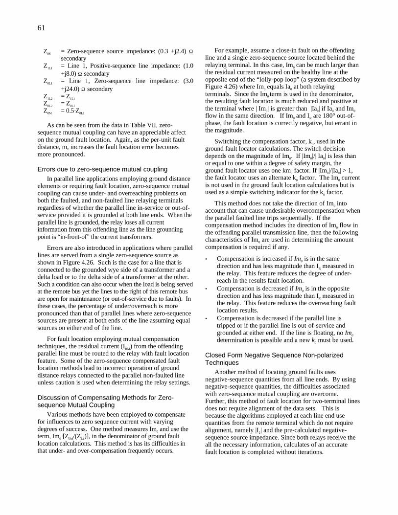
61
Z0S = Zero-sequence source impedance: (0.3 +j2.4) Ω secondary
Z1L1 = Line 1, Positive-sequence line impedance: (1.0 +j8.0) Ω secondary
Z0L1 = Line 1, Zero-sequence line impedance: (3.0 +j24.0) Ω secondary
Z1L2 = Z1L1 Z0L2 = Z0L1 Z0M = 0.5·Z0L1
As can be seen from the data in Table VII, zero-sequence mutual coupling can have an appreciable affect on the ground fault location. Again, as the per-unit fault distance, m, increases the fault location error becomes more pronounced.
Errors due to zero-sequence mutual coupling In parallel line applications employing ground distance
elements or requiring fault location, zero-sequence mutual coupling can cause under- and overreaching problems on both the faulted, and non-faulted line relaying terminals regardless of whether the parallel line in-service or out-of-service provided it is grounded at both line ends. When the parallel line is grounded, the relay loses all current information from this offending line as the line grounding point is “in-front-of” the current transformers.
Errors are also introduced in applications where parallel lines are served from a single zero-sequence source as shown in Figure 4.26. Such is the case for a line that is connected to the grounded wye side of a transformer and a delta load or to the delta side of a transformer at the other. Such a condition can also occur when the load is being served at the remote bus yet the lines to the right of this remote bus are open for maintenance (or out-of-service due to faults). In these cases, the percentage of under/overreach is more pronounced than that of parallel lines where zero-sequence sources are present at both ends of the line assuming equal sources on either end of the line.
For fault location employing mutual compensation techniques, the residual current (IRM) from the offending parallel line must be routed to the relay with fault location feature. Some of the zero-sequence compensated fault location methods lead to incorrect operation of ground distance relays connected to the parallel non-faulted line unless caution is used when determining the relay settings.
Discussion of Compensating Methods for Zero-sequence Mutual Coupling
Various methods have been employed to compensate for influences to zero sequence current with varying degrees of success. One method measures Im0 and use the term, Im0·[Z0M/(ZL1)], in the denominator of ground fault location calculations. This method is has its difficulties in that under- and over-compensation frequently occurs.
For example, assume a close-in fault on the offending line and a single zero-sequence source located behind the relaying terminal. In this case, Im0 can be much larger than the residual current measured on the healthy line at the opposite end of the “lolly-pop loop” (a system described by Figure 4.26) where Im0 equals Ia0 at both relaying terminals. Since the Im0 term is used in the denominator, the resulting fault location is much reduced and positive at the terminal where | Im0| is greater than |Ia0| if Ia0 and Im0 flow in the same direction. If Im0 and IR are 180° out-of-phase, the fault location is correctly negative, but errant in the magnitude.
Switching the compensation factor, k0, used in the ground fault locator calculations. The switch decision depends on the magnitude of Im0. If |Im0|/| Ia0| is less than or equal to one within a degree of safety margin, the ground fault locator uses one km0 factor. If |Im0|/|Ia0| > 1, the fault locator uses an alternate k0 factor. The Im0 current is not used in the ground fault location calculations but is used as a simple switching indicator for the k0 factor.
This method does not take the direction of Im0 into account that can cause undesirable overcompensation when the parallel faulted line trips sequentially. If the compensation method includes the direction of Im0 flow in the offending parallel transmission line, then the following characteristics of Im0 are used in determining the amount compensation is required if any.
• Compensation is increased if Im0 is in the same direction and has less magnitude than IR measured in the relay. This feature reduces the degree of under-reach in the results fault location.
• Compensation is decreased if Im0 is in the opposite direction and has less magnitude than IR measured in the relay. This feature reduces the overreaching fault location results.
• Compensation is decreased if the parallel line is tripped or if the parallel line is out-of-service and grounded at either end. If the line is floating, no Im0 determination is possible and a new k0 must be used.
Closed Form Negative Sequence Non-polarized Techniques
Another method of locating ground faults uses negative-sequence quantities from all line ends. By using negative-sequence quantities, the difficulties associated with zero-sequence mutual coupling are overcome. Further, this method of fault location for two-terminal lines does not require alignment of the data sets. This is because the algorithms employed at each line end use quantities from the remote terminal which do not require alignment, namely |I2| and the pre-calculated negative-sequence source impedance. Since both relays receive the all the necessary information, calculates of an accurate fault location is completed without iterations.
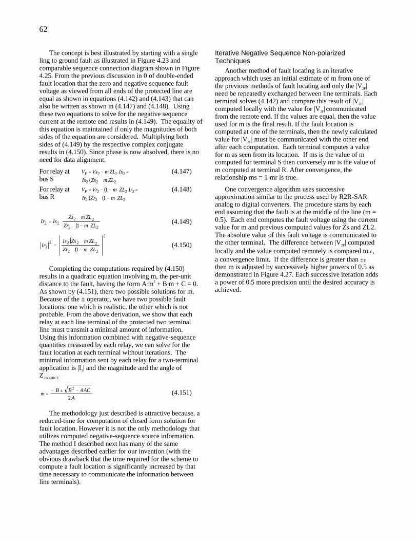
62
The concept is best illustrated by starting with a single ling to ground fault as illustrated in Figure 4.23 and comparable sequence connection diagram shown in Figure 4.25. From the previous discussion in 0 of double-ended fault location that the zero and negative sequence fault voltage as viewed from all ends of the protected line are equal as shown in equations (4.142) and (4.143) that can also be written as shown in (4.147) and (4.148). Using these two equations to solve for the negative sequence current at the remote end results in (4.149). The equality of this equation is maintained if only the magnitudes of both sides of the equation are considered. Multiplying both sides of (4.149) by the respective complex conjugate results in (4.150). Since phase is now absolved, there is no need for data alignment.
For relay at bus S ( )222
222
ZLmZsIs
IsZLmVsVF
+
=−=
(4.147)
For relay at bus R
( )( )( )222
222
1
1
ZLmZrIr
IrZLmVrVF
−+
=−−=
(4.148)
( )
−+
+=
22
2222 1 ZLmZr
ZLmZsIsIr (4.149)
( )( )
2
22
22222 1
−+
+=
ZLmZr
ZLmZsIsIr (4.150)
Completing the computations required by (4.150)
results in a quadratic equation involving m, the per-unit distance to the fault, having the form A·m2 + B·m + C = 0. As shown by (4.151), there two possible solutions for m. Because of the ± operator, we have two possible fault locations: one which is realistic, the other which is not probable. From the above derivation, we show that each relay at each line terminal of the protected two terminal line must transmit a minimal amount of information. Using this information combined with negative-sequence quantities measured by each relay, we can solve for the fault location at each terminal without iterations. The minimal information sent by each relay for a two-terminal application is |I2| and the magnitude and the angle of Z2SOURCE
A
ACBBm
2
42 −±−= (4.151)
The methodology just described is attractive because, a
reduced-time for computation of closed form solution for fault location. However it is not the only methodology that utilizes computed negative-sequence source information. The method I described next has many of the same advantages described earlier for our invention (with the obvious drawback that the time required for the scheme to compute a fault location is significantly increased by that time necessary to communicate the information between line terminals).
Iterative Negative Sequence Non-polarized Techniques
Another method of fault locating is an iterative approach which uses an initial estimate of m from one of the previous methods of fault locating and only the |V2F| need be repeatedly exchanged between line terminals. Each terminal solves (4.142) and compare this result of |V2F| computed locally with the value for |V2F| communicated from the remote end. If the values are equal, then the value used for m is the final result. If the fault location is computed at one of the terminals, then the newly calculated value for |V2F| must be communicated with the other end after each computation. Each terminal computes a value for m as seen from its location. If ms is the value of m computed for terminal S then conversely mr is the value of m computed at terminal R. After convergence, the relationship ms = 1-mr is true.
One convergence algorithm uses successive approximation similar to the process used by R2R-SAR analog to digital converters. The procedure starts by each end assuming that the fault is at the middle of the line (m = 0.5). Each end computes the fault voltage using the current value for m and previous computed values for Zs and ZL2. The absolute value of this fault voltage is communicated to the other terminal. The difference between |V2F| computed locally and the value computed remotely is compared to ε, a convergence limit. If the difference is greater than ±ε then m is adjusted by successively higher powers of 0.5 as demonstrated in Figure 4.27. Each successive iteration adds a power of 0.5 more precision until the desired accuracy is achieved.
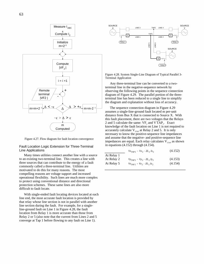
63
Measure IABC
&Compute I2
Initializem=2-1
Compute|VF2 |
Remoteterminal|VF2 |
m=m+2 -i
+-
∆ m=m-2 -i
i = i +1
−ε > ∆ > ε
mComputed
∆ < -ε ∆ > +ε
Figure 4.27. Flow diagram for fault location convergence
Fault Location Logic Extension for Three-Terminal Line Applications
Many times utilities connect another line with a source to an existing two-terminal line. This creates a line with three sources that can contribute to the energy of a fault commonly called a three-terminal line. Utilities are motivated to do this for many reasons. The most compelling reasons are voltage support and increased operational flexibility. Such lines are much more complex to protect using conventional distance and directional protection schemes. These same lines are also more difficult to fault locate.
With single-ended fault locating devices located at each line end, the most accurate fault location is provided by that relay whose line section is not in parallel with another line section during the fault. For example, for a single-line-ground fault on Line 1 in Figure 4.28, the fault location from Relay 1 is more accurate than those from Relay 2 or 5 (also note that the current from Lines 2 and 5 converge at Tap 1 before flowing to any fault on Line 1).
1
Relay 1
2
Relay 2
Relay 5
5
SOURCEX
SOURCEY
SOURCEZ
TAP1
TAP2
LINE 1 LINE 2
LINE 3 LINE 4
LIN
E 5
LIN
E 6
Figure 4.28. System Single-Line Diagram of Typical Parallel 3-Terminal Application
Any three-terminal line can be converted to a two-terminal line in the negative-sequence network by observing the following points in the sequence connection diagram of Figure 4.29. The parallel portion of the three-terminal line has been reduced to a single line to simplify the diagram and explanation without loss of accuracy.
The sequence connection diagram in Figure 4.29 assumes a single-line-ground fault located m per-unit distance from Bus X that is connected to Source X. With this fault placement, there are two voltages that the Relays 2 and 5 calculate the same: VF2 and V TAP2. Exact knowledge of the fault location on Line 1 is not required to accurately calculate V2TAP at Relay 2 and 5. It is only necessary to know the positive-sequence line impedances and assume that the negative- and positive-sequence line impedances are equal. Each relay calculates V2TAP as shown in equations (4.152) through (4.154).
At Relay 1 2222 IxZLVxVxTAP −= (4.152)
At Relay 2 2222 IyZLVyVyTAP −= (4.153) At Relay 5 2222 IzZLVzVzTAP −= (4.154)
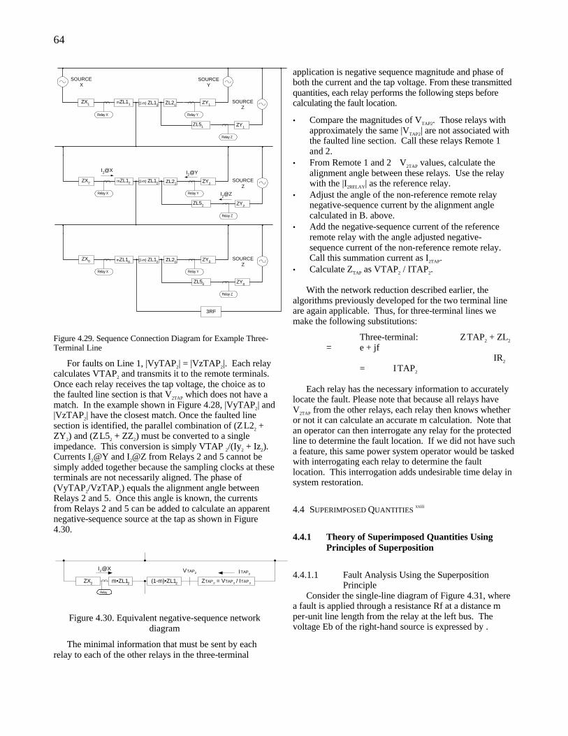
64
3RF
I2@Z
mZL11ZX1
SOURCEX
Relay X
ZY1
SOURCEY
Relay Y
ZY1
SOURCEZ
Relay Z
ZL51
ZL21
mZL12ZX2
Relay X
ZY2
Relay Y
ZY2
SOURCEZ
Relay Z
ZL52
ZL22(1-m) ZL12
ZX0
Relay X
ZY0
Relay Y
ZY0
SOURCEZ
Relay Z
ZL50
ZL20
(1-m) ZL12
mZL10 (1-m) ZL12
I2@YI2@X
Figure 4.29. Sequence Connection Diagram for Example Three-Terminal Line
For faults on Line 1, |VyTAP2| = |VzTAP2|. Each relay calculates VTAP2 and transmits it to the remote terminals. Once each relay receives the tap voltage, the choice as to the faulted line section is that V2TAP which does not have a match. In the example shown in Figure 4.28, |VyTAP2| and |VzTAP2| have the closest match. Once the faulted line section is identified, the parallel combination of (Z L22 + ZY2) and (Z L52 + ZZ2) must be converted to a single impedance. This conversion is simply VTAP 2/(Iy2 + Iz2). Currents I2@Y and I2@Z from Relays 2 and 5 cannot be simply added together because the sampling clocks at these terminals are not necessarily aligned. The phase of (VyTAP2/VzTAP2) equals the alignment angle between Relays 2 and 5. Once this angle is known, the currents from Relays 2 and 5 can be added to calculate an apparent negative-sequence source at the tap as shown in Figure 4.30.
ZX2 m•ZL12 (1-m)•ZL12 ZTAP2 = VTAP2 / ITAP2
Relay
I2@X VTAP2 ITAP2
Figure 4.30. Equivalent negative-sequence network diagram
The minimal information that must be sent by each relay to each of the other relays in the three-terminal
application is negative sequence magnitude and phase of both the current and the tap voltage. From these transmitted quantities, each relay performs the following steps before calculating the fault location.
• Compare the magnitudes of VTAP2. Those relays with approximately the same |VTAP2| are not associated with the faulted line section. Call these relays Remote 1 and 2.
• From Remote 1 and 2 ∠V2TAP values, calculate the alignment angle between these relays. Use the relay with the |I2RELAY| as the reference relay.
• Adjust the angle of the non-reference remote relay negative-sequence current by the alignment angle calculated in B. above.
• Add the negative-sequence current of the reference remote relay with the angle adjusted negative-sequence current of the non-reference remote relay. Call this summation current as I2TAP.
• Calculate ZTAP as VTAP2 / ITAP2.
With the network reduction described earlier, the algorithms previously developed for the two terminal line are again applicable. Thus, for three-terminal lines we make the following substitutions:
Three-terminal: Z TAP2 + ZL2
= e + jf IR2
= I TAP2
Each relay has the necessary information to accurately locate the fault. Please note that because all relays have V2TAP from the other relays, each relay then knows whether or not it can calculate an accurate m calculation. Note that an operator can then interrogate any relay for the protected line to determine the fault location. If we did not have such a feature, this same power system operator would be tasked with interrogating each relay to determine the fault location. This interrogation adds undesirable time delay in system restoration.
4.4 SUPERIMPOSED QUANTITIES xxiii
4.4.1 Theory of Superimposed Quantities Using Principles of Superposition
4.4.1.1 Fault Analysis Using the Superposition Principle
Consider the single-line diagram of Figure 4.31, where a fault is applied through a resistance Rf at a distance m per-unit line length from the relay at the left bus. The voltage Eb of the right-hand source is expressed by .
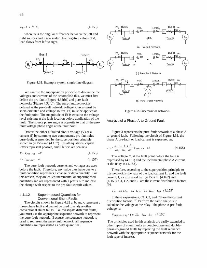
65
sj
R EehE ⋅⋅= − θ (4.155)
where Θ is the angular difference between the left and right sources and h is a scalar. For negative values of Θ, load flows from left to right.
Bus S
52
ZL1
ES
ZS1
ER
ZR1
Bus R
52
Relay S Relay R
Figure 4.31. Example system single-line diagram
We can use the superposition principle to determine the
voltages and currents of the accomplish this, we must first define the pre-fault (Figure 4.32(b)) and pure-fault networks (Figure 4.32(c)). The pure-fault network is defined as the pre-fault network voltage sources must be short-circuited and voltage source, Ef, must be applied at the fault point. The magnitude of Ef is equal to the voltage level existing at the fault location before application of the fault. The source phase angle is opposite to that of the pre-fault voltage phase angle at the fault point.
Determine either a faulted circuit voltage (V) or a current (I) by summing two components, pre-fault plus pure-fault, as provided by the superposition principle shown in (4.156) and (4.157). (In all equations, capital letters represent phasors, small letters are scalars)
VVV FLTPRE ∆+= − (4.156)
III FLTPRE ∆+= − (4.157)
The pure-fault network currents and voltages are zero before the fault. Therefore, any value they have due to a fault condition represents a change or delta quantity. For this reason, they are called incremental or superimposed quantities and are represented with a prefix ∆ to indicate the change with respect to the pre-fault circuit values.
4.4.1.2 Superimposed Quantities for Conventional Shunt Faults
The circuits shown in Figure 4.32 a, b, and c represent a three-phase fault and cannot be used to analyze other conventional shunt faults. To investigate different faults, you must use the appropriate sequence network to represent the pure-fault network. Because the sequence network is used to represent the pure-fault network, all sequence quantities are represented as delta quantities.
Bus S
52
mZL1
ES
ZS1
ER
ZR1Bus R
52
(1-m)ZL1
Relay S Relay RRF
Bus S
52
mZL1
ES
ZS1
ER
ZR1Bus R
52
(1-m)ZL1
Relay S Relay REFILD
Bus S
52
mZL1ZS1 ZR1
Bus R
52
(1-m)ZL1
Relay S Relay R
RF
EF
-+
(c) Pure - Fault Network
(b) Pre - Fault Network
(a) Faulted Network
∆V ∆ I
Figure 4.32. Superposition networks
Analysis of a Phase A-to-Ground Fault
Figure 3 represents the pure-fault network of a phase A-
to-ground fault. Following the circuit of Figure 4.31, the phase A pre-fault or load current is expressed as:
IIZRZLZS
ehEI FLTPRE
jS
LD ∆+++
⋅−⋅= −
−
111
)1( θ
(4.158)
The voltage EF at the fault point before the fault is expressed by (4.161) and the incremental phase A current, at the relay as (4.162).
Therefore, according to the superposition principle to this network is the sum of the load current ILD and the fault current, IF as expressed by (4.159). In (4.162) and (4.159), C1, C2, and C0 are the current distribution factors [9].
LDFFFAR IICICICI +∆⋅+∆⋅+∆⋅= 021 021 (4.159)
In these expressions, C1, C2, and C0 are the current distribution factors. xxiv Perform the same analysis to calculate the voltage at the relay. The phase A pre-fault voltage is:
( ) FLDFLTPREAR EIZLmV +⋅⋅=− 1)( (4.160)
The principles used in this analysis are easily extended to other types of shunt faults as double-phase and double-phase-to-ground faults by replacing the fault sequence network with the appropriate sequence network for the fault type of interest.
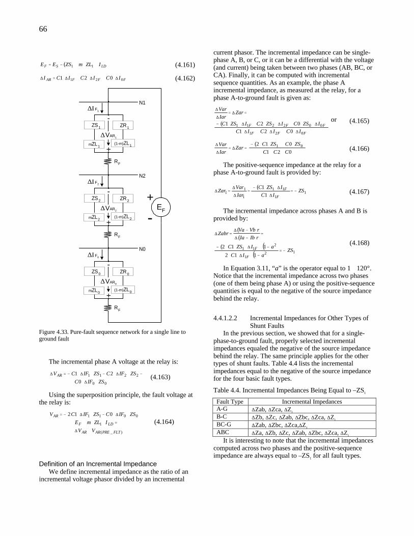
66
( ) LDSF IZLmZSEE ⋅⋅+−= 11 (4.161)
FFFAR ICICICI 021 021 ∆⋅+∆⋅+∆⋅=∆ (4.162)
mZL1
ZS1
(1-m)ZL1
ZR1
-
+
∆VAR1
∆Ι F1
RF
N1
mZL2
ZS2
(1-m)ZL2
ZR2
-
+
∆VAR2
∆Ι F2
RF
N2
mZL0
ZS0
(1-m)ZL0
ZR0
-
+
∆VAR0
∆Ι F0
RF
N0
EF
-+
Figure 4.33. Pure-fault sequence network for a single line to ground fault
The incremental phase A voltage at the relay is:
00
2211
0
21
ZSIFC
ZSIFCZSIFCVAR
⋅∆⋅
−⋅∆⋅−⋅∆⋅−=∆ (4.163)
Using the superposition principle, the fault voltage at the relay is:
)_(
1
0011 012
FLTPREARAR
LDF
AR
VV
IZLmE
ZSIFCZSIFCV
+∆
=⋅⋅+
+⋅∆⋅−⋅∆⋅−=
(4.164)
Definition of an Incremental Impedance We define incremental impedance as the ratio of an
incremental voltage phasor divided by an incremental
current phasor. The incremental impedance can be single-phase A, B, or C, or it can be a differential with the voltage (and current) being taken between two phases (AB, BC, or CA). Finally, it can be computed with incremental sequence quantities. As an example, the phase A incremental impedance, as measured at the relay, for a phase A-to-ground fault is given as:
( )FFF
FFF
ICICIC
IZSCIZSCIZSC
ZarIar
Var
021
002211
021
021
∆⋅+∆⋅+∆⋅
∆⋅⋅+∆⋅⋅+∆⋅⋅−
=∆=∆
∆
or (4.165)
( )021
012 01
CCC
ZSCZSCZar
Iar
Var
++
⋅+⋅⋅⋅−=∆=
∆
∆ (4.166)
The positive-sequence impedance at the relay for a phase A-to-ground fault is provided by:
( )1
1
11
1
11 1
1ZS
IC
IZSC
Iar
VarZar
F
F −=∆⋅
∆⋅⋅−=
∆
∆=∆ (4.167)
The incremental impedance across phases A and B is provided by:
( )( )
( ) ( )( ) 12
1
211
112
112ZS
aIC
aIZSC
rIbIa
rVbVaZabr
F
F −=−⋅∆⋅⋅
−⋅∆⋅⋅⋅−
=−∆
−∆=∆
(4.168)
In Equation 3.11, “a” is the operator equal to 1∠ 120°. Notice that the incremental impedance across two phases (one of them being phase A) or using the positive-sequence quantities is equal to the negative of the source impedance behind the relay.
4.4.1.2.2 Incremental Impedances for Other Types of Shunt Faults
In the previous section, we showed that for a single-phase-to-ground fault, properly selected incremental impedances equaled the negative of the source impedance behind the relay. The same principle applies for the other types of shunt faults. Table 4.4 lists the incremental impedances equal to the negative of the source impedance for the four basic fault types.
Table 4.4. Incremental Impedances Being Equal to –ZS1
Fault Type Incremental Impedances A-G ∆Zab, ∆Zca, ∆Z1 B-C ∆Zb, ∆Zc, ∆Zab, ∆Zbc, ∆Zca, ∆Z1 BC-G ∆Zab, ∆Zbc, ∆Zca,∆Z1 ABC ∆Za, ∆Zb, ∆Zc, ∆Zab, ∆Zbc, ∆Zca, ∆Z1
It is interesting to note that the incremental impedances computed across two phases and the positive-sequence impedance are always equal to –ZS1 for all fault types.
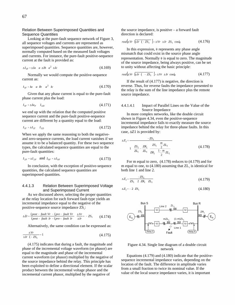
67
Relation Between Superimposed Quantities and Sequence Quantities
Looking at the pure-fault sequence network of Figure 3, all sequence voltages and currents are represented as superimposed quantities. Sequence quantities are, however, normally computed based on the measured fault voltages and currents. For instance, the pure-fault positive-sequence current at the fault is provided as:
IcaIbaIaI F ∆⋅+∆⋅+∆=∆ 21 (4.169)
Normally we would compute the positive-sequence current as:
IcaIbaIaI F ⋅+⋅+= 21 (4.170)
Given that any phase current is equal to the pure-fault phase current plus the load:
LDFF IIaI +∆=1 (4.171)
we end up with the relation that the computed positive sequence current and the pure-fault positive-sequence current are different by a quantity equal to the load:
LDFF III +∆= 11 (4.172)
When we apply the same reasoning to both the negative- and zero-sequence currents, the load current vanishes if we assume it to be a balanced quantity. For these two sequence types, the calculated sequence quantities are equal to the pure-fault quantities:
FF II 22 ∆= and FF II 00 ∆= (4.173)
In conclusion, with the exception of positive-sequence quantities, the calculated sequence quantities are superimposed quantities.
4.4.1.3 Relation Between Superimposed Voltage and Superimposed Current
As we discussed above, selecting the proper quantities at the relay location for each forward fault-type yields an incremental impedance equal to the negative of the positive-sequence source impedance ZS1:
( ) ( )( ) ( ) 1ZS
Ir
Vr
IrfaultpreIrfaultpost
VrfaultpreVrfaultpostZr −=
∆
∆
−−−
−−−=∆ (4.174)
Alternatively, the same condition can be expressed as:
( )1
1=
−⋅∆
∆
ZSIr
Vr (4.175)
(4.175) indicates that during a fault, the magnitude and phase of the incremental voltage waveform (or phasor) are equal to the magnitude and phase of the incremental current waveform (or phasor) multiplied by the negative of the source impedance behind the relay. This principle has been exploited to define a directional element. If the scalar product between the incremental voltage phasor and the incremental current phasor, multiplied by the negative of
the source impedance, is positive – a forward fault direction is declared:
( )( )[ ] ( )θcos11 ⋅⋅∆⋅∆=−⋅∆⋅∆ ZSIrVrZSIrVrreal (4.176)
In this expression, θ represents any phase angle mismatch that could exist in the source phase angle representation. Normally θ is equal to zero. The magnitude of the source impedance, being always positive, can be set to unity without affecting the basic principle:
( )( )[ ] ( )θcos1 ⋅∆⋅∆=−∠⋅∆⋅∆ IrVrZSIrVrreal (4.177)
If the result of (4.177) is negative, the direction is reverse. Thus, for reverse faults the impedance presented to the relay is the sum of the line impedance plus the remote source impedance.
4.4.1.4.1 Impact of Parallel Lines on the Value of the Source Impedance
In more complex networks, like the double circuit shown in Figure 4.34, even the positive-sequence incremental impedance fails to exactly measure the source impedance behind the relay for three-phase faults. In this case, ∆Z1 is provided by:
−+
+−+
−=∆
11
11
1
1
1
1
11
21
21ZL
mZR
ZLm
ZS
ZL
ZR
ZL
ZS
ZSZ
(4.178)
For m equal to zero, (4.178) reduces to (4.179) and for m equal to one, to (4.180) assuming that ZL1 is identical for both line 1 and line 2.
111
11 2 ZLZRZS
ZSZ
+⋅+
−=∆ (4.179)
11 2 ZSZ ⋅−=∆ (4.180)
Fault
52
mZL1
Bus R
52
Relay S Relay R
(1-m)ZL1
52 52
Bus SZL1
Line 1
Line 2
ES
ZS1
ER
ZR1
Figure 4.34. Single line diagram of a double circuit network
Equations (4.179) and (4.180) indicate that the positive-sequence incremental impedance varies, depending on the location of the fault. The difference in amplitude varies from a small fraction to twice its nominal value. If the value of the local source impedance varies, it is important
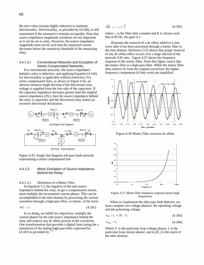
68
the new value remains highly inductive to maintain directionality. Directionality, as provided by (4.166), is still maintained if the mismatch θ remains acceptable. Note that source impedance magnitude variations are not important as it can be set to unity. However, the source impedance magnitude must not be such that the measured current decreases below the sensitivity threshold of the measuring relay.
4.4.1.4.2 Conventional Networks and Exception of Series Compensated Networks
For conventional networks, the source impedance behind a relay is inductive, and applying Equation (4.166) for directionality is applicable without restriction. For series compensated lines, as shown in Figure 4.35, an adverse situation might develop if the directional relay voltage is supplied from the line side of the capacitors. If the capacitor impedance becomes greater than the original source impedance (ZS1), then the source impedance behind the relay is capacitive and the directional relay makes an incorrect directional declaration.
Bus S
52
mZL1ZS1 ZR1
Bus R
52
(1-m)ZL1
Relay S Relay R
RF
EF
-+
(b) Pure - Fault Network
∆V
∆ I
XC
52
ZL1
ESZS1
ERZR1
Bus R
52
Relay S Relay R
Bus S
XC
(a) Single Line Diageam
Figure 4.35. Single line diagram and pure-fault network representing a series compensated line
4.4.1.5 Mimic Emulation of Source Impedance Behind the Relay
4.4.1.5.1 Definition of a Mimic Filter In Equation 5.3, the negative of the unit source
impedance behind the relay, to get a compensated current, must multiply the incremental current phasor. This can be accomplished in the time domain by processing the current waveform through a high-pass filter, or mimic, of the form:
( )sK 11 τ+ (4.181)
In so doing, we fulfill two objectives: multiply the current phasor by the unit source impedance behind the relay and remove any dc offset present in the waveform. One transformation that provides a digital form (using the z transform) of the analog high-pass filter expressed by (4.181) is provided by: xxiv
( )[ ]1111 −−+ zK ττ (4.182)
where τ1 is the filter time constant and K is chosen such that at 60 Hz, the gain is 1.
illustrates the removal of a dc offset added to a sine wave after it has been processed through a mimic filter in the time domain. Reference [12] shows that proper removal of any dc-offset effect occurs over a large interval of the network X/R ratio. Figure 4.37 shows the frequency response of the mimic filter. From this figure, notice that the mimic filter is a high-pass filter. While the mimic filter does remove dc from the original waveform, the higher frequency components (if they exist) are amplified.
Figure 4.36 Mimic Filter removes dc-offset
Figure 4.37. Mimic filter frequency response passes high
frequencies
When we implement the mho type fault detector, we must compute two voltage phasors: the operating voltage and the polarizing voltage:
rrOP VZLkIS −⋅⋅= 1 (4.183)
rPOL VS = (4.184)
Where Vr is the particular loop voltage phasor, Ir is the particular loop current phasor, and k (ZL1) is the reach of the mho element.
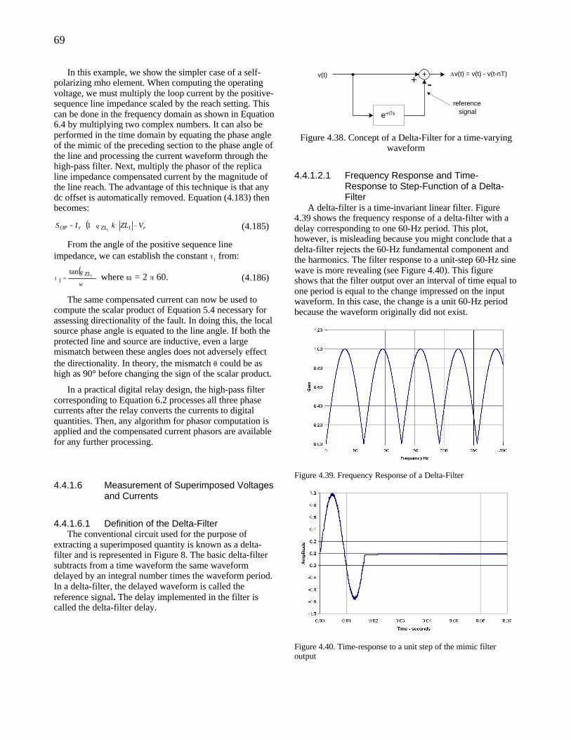
69
In this example, we show the simpler case of a self-polarizing mho element. When computing the operating voltage, we must multiply the loop current by the positive-sequence line impedance scaled by the reach setting. This can be done in the frequency domain as shown in Equation 6.4 by multiplying two complex numbers. It can also be performed in the time domain by equating the phase angle of the mimic of the preceding section to the phase angle of the line and processing the current waveform through the high-pass filter. Next, multiply the phasor of the replica line impedance compensated current by the magnitude of the line reach. The advantage of this technique is that any dc offset is automatically removed. Equation (4.183) then becomes:
( ) rZLrOP VZLkIS −⋅∠⋅= 111 θ (4.185)
From the angle of the positive sequence line impedance, we can establish the constant τ1 from:
( )ω
θτ 1
tan1
ZL= where ω = 2 π 60. (4.186)
The same compensated current can now be used to compute the scalar product of Equation 5.4 necessary for assessing directionality of the fault. In doing this, the local source phase angle is equated to the line angle. If both the protected line and source are inductive, even a large mismatch between these angles does not adversely effect the directionality. In theory, the mismatch θ could be as high as 90° before changing the sign of the scalar product.
In a practical digital relay design, the high-pass filter corresponding to Equation 6.2 processes all three phase currents after the relay converts the currents to digital quantities. Then, any algorithm for phasor computation is applied and the compensated current phasors are available for any further processing.
4.4.1.6 Measurement of Superimposed Voltages and Currents
4.4.1.6.1 Definition of the Delta-Filter The conventional circuit used for the purpose of
extracting a superimposed quantity is known as a delta-filter and is represented in Figure 8. The basic delta-filter subtracts from a time waveform the same waveform delayed by an integral number times the waveform period. In a delta-filter, the delayed waveform is called the reference signal. The delay implemented in the filter is called the delta-filter delay.
+
e-nTs
v(t) ∆v(t) = v(t) - v(t-nT)
-+
referencesignal
Figure 4.38. Concept of a Delta-Filter for a time-varying waveform
4.4.1.2.1 Frequency Response and Time-Response to Step-Function of a Delta-Filter
A delta-filter is a time-invariant linear filter. Figure 4.39 shows the frequency response of a delta-filter with a delay corresponding to one 60-Hz period. This plot, however, is misleading because you might conclude that a delta-filter rejects the 60-Hz fundamental component and the harmonics. The filter response to a unit-step 60-Hz sine wave is more revealing (see Figure 4.40). This figure shows that the filter output over an interval of time equal to one period is equal to the change impressed on the input waveform. In this case, the change is a unit 60-Hz period because the waveform originally did not exist.
Figure 4.39. Frequency Response of a Delta-Filter
Figure 4.40. Time-response to a unit step of the mimic filter output
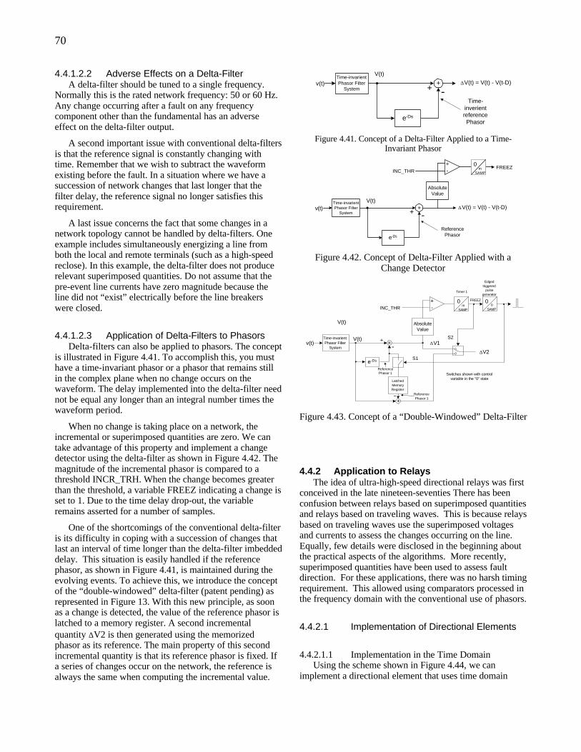
70
4.4.1.2.2 Adverse Effects on a Delta-Filter A delta-filter should be tuned to a single frequency.
Normally this is the rated network frequency: 50 or 60 Hz. Any change occurring after a fault on any frequency component other than the fundamental has an adverse effect on the delta-filter output.
A second important issue with conventional delta-filters is that the reference signal is constantly changing with time. Remember that we wish to subtract the waveform existing before the fault. In a situation where we have a succession of network changes that last longer that the filter delay, the reference signal no longer satisfies this requirement.
A last issue concerns the fact that some changes in a network topology cannot be handled by delta-filters. One example includes simultaneously energizing a line from both the local and remote terminals (such as a high-speed reclose). In this example, the delta-filter does not produce relevant superimposed quantities. Do not assume that the pre-event line currents have zero magnitude because the line did not “exist” electrically before the line breakers were closed.
4.4.1.2.3 Application of Delta-Filters to Phasors Delta-filters can also be applied to phasors. The concept
is illustrated in Figure 4.41. To accomplish this, you must have a time-invariant phasor or a phasor that remains still in the complex plane when no change occurs on the waveform. The delay implemented into the delta-filter need not be equal any longer than an integral number times the waveform period.
When no change is taking place on a network, the incremental or superimposed quantities are zero. We can take advantage of this property and implement a change detector using the delta-filter as shown in Figure 4.42. The magnitude of the incremental phasor is compared to a threshold INCR_TRH. When the change becomes greater than the threshold, a variable FREEZ indicating a change is set to 1. Due to the time delay drop-out, the variable remains asserted for a number of samples.
One of the shortcomings of the conventional delta-filter is its difficulty in coping with a succession of changes that last an interval of time longer than the delta-filter imbedded delay. This situation is easily handled if the reference phasor, as shown in Figure 4.41, is maintained during the evolving events. To achieve this, we introduce the concept of the “double-windowed” delta-filter (patent pending) as represented in Figure 13. With this new principle, as soon as a change is detected, the value of the reference phasor is latched to a memory register. A second incremental quantity ∆V2 is then generated using the memorized phasor as its reference. The main property of this second incremental quantity is that its reference phasor is fixed. If a series of changes occur on the network, the reference is always the same when computing the incremental value.
+
e-Ds
v(t) ∆V(t) = V(t) - V(t-D)
-+Time-
inverientreferencePhasor
Time-invarientPhasor Filter
System
V(t)
Figure 4.41. Concept of a Delta-Filter Applied to a Time-
Invariant Phasor
+
e-Ds
v(t) ∆V(t) = V(t) - V(t-D)
-+
ReferencePhasor
Time-invarientPhasor Filter
System
AbsoluteValue
0- m
SAMP
+FREEZ
INC_THR
V(t)
Figure 4.42. Concept of Delta-Filter Applied with a Change Detector
∆V1-
ReferencePhasor 1
AbsoluteValue
0- m
SAMP
+ FREEZ
INC_THR
v(t)Time-invarientPhasor Filter
System
V(t)
+
e-Ds
+
LatchedMemoryRegister
00
SAMP
-+
ReferencePhasor 1
V(t)
S1
S2
∆V2
Timer 1
Edgedtriggered
pulsegenerator
Switches shown with controlvariable in the "0" state
Figure 4.43. Concept of a “Double-Windowed” Delta-Filter
4.4.2 Application to Relays The idea of ultra-high-speed directional relays was first
conceived in the late nineteen-seventies There has been confusion between relays based on superimposed quantities and relays based on traveling waves. This is because relays based on traveling waves use the superimposed voltages and currents to assess the changes occurring on the line. Equally, few details were disclosed in the beginning about the practical aspects of the algorithms. More recently, superimposed quantities have been used to assess fault direction. For these applications, there was no harsh timing requirement. This allowed using comparators processed in the frequency domain with the conventional use of phasors.
4.4.2.1 Implementation of Directional Elements
4.4.2.1.1 Implementation in the Time Domain Using the scheme shown in Figure 4.44, we can
implement a directional element that uses time domain
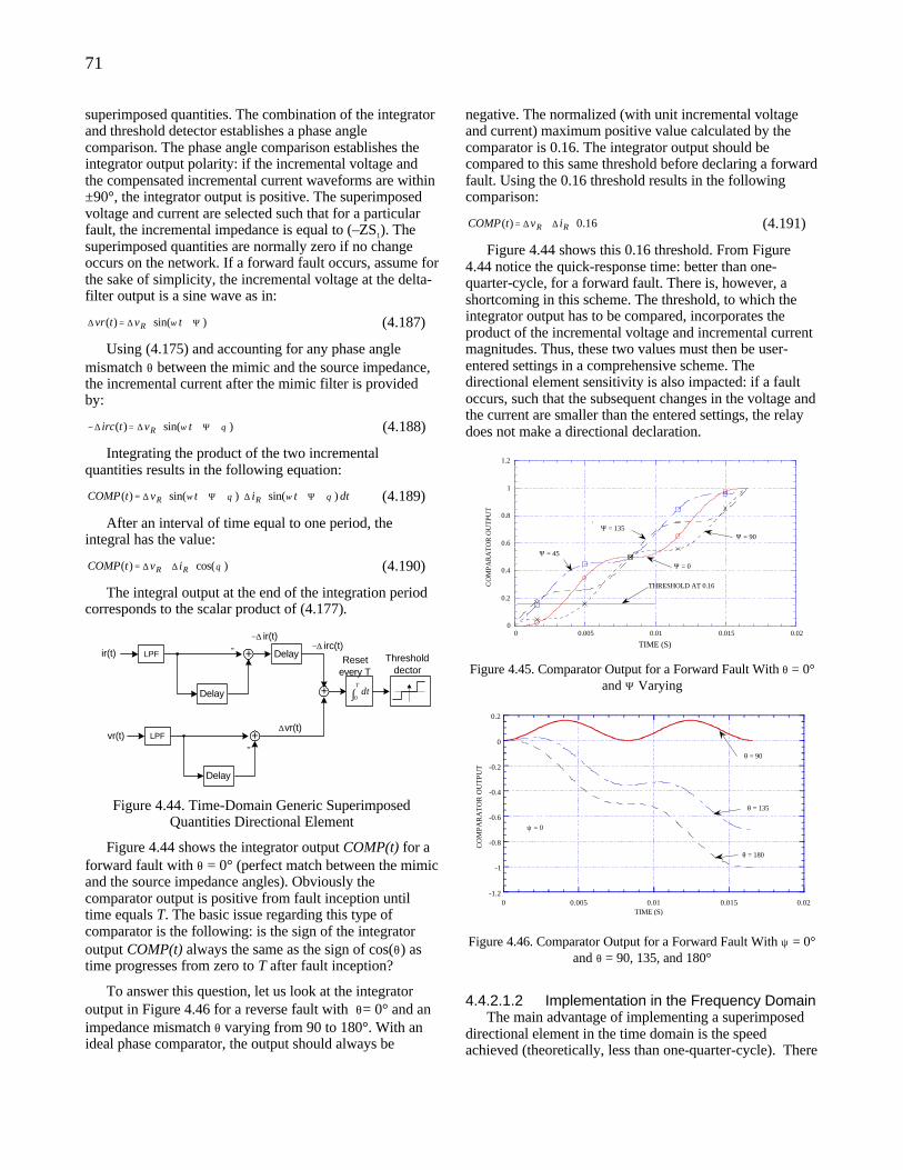
71
superimposed quantities. The combination of the integrator and threshold detector establishes a phase angle comparison. The phase angle comparison establishes the integrator output polarity: if the incremental voltage and the compensated incremental current waveforms are within ±90°, the integrator output is positive. The superimposed voltage and current are selected such that for a particular fault, the incremental impedance is equal to (–ZS1). The superimposed quantities are normally zero if no change occurs on the network. If a forward fault occurs, assume for the sake of simplicity, the incremental voltage at the delta-filter output is a sine wave as in:
)sin()( Ψ+⋅∆=∆ tvtvr R ω (4.187)
Using (4.175) and accounting for any phase angle mismatch θ between the mimic and the source impedance, the incremental current after the mimic filter is provided by:
)sin()( θω +Ψ+⋅∆=∆− tvtirc R (4.188)
Integrating the product of the two incremental quantities results in the following equation:
dttitvtCOMP RR )sin()sin()( θωθω +Ψ+⋅∆⋅+Ψ+⋅∆= (4.189)
After an interval of time equal to one period, the integral has the value:
)cos()( θ⋅∆⋅∆= RR ivtCOMP (4.190)
The integral output at the end of the integration period corresponds to the scalar product of (4.177).
+
Delay
-LPF Delay
+
+
Delay
-LPF
∫T
dt0
`
Thresholddector
Resetevery T
∆vr(t)vr(t)
ir(t)
−∆ ir(t)−∆ irc(t)
Figure 4.44. Time-Domain Generic Superimposed Quantities Directional Element
Figure 4.44 shows the integrator output COMP(t) for a forward fault with θ = 0° (perfect match between the mimic and the source impedance angles). Obviously the comparator output is positive from fault inception until time equals T. The basic issue regarding this type of comparator is the following: is the sign of the integrator output COMP(t) always the same as the sign of cos(θ) as time progresses from zero to T after fault inception?
To answer this question, let us look at the integrator output in Figure 4.46 for a reverse fault with θ= 0° and an impedance mismatch θ varying from 90 to 180°. With an ideal phase comparator, the output should always be
negative. The normalized (with unit incremental voltage and current) maximum positive value calculated by the comparator is 0.16. The integrator output should be compared to this same threshold before declaring a forward fault. Using the 0.16 threshold results in the following comparison:
16.0)( ⋅∆⋅∆= RR ivtCOMP (4.191)
Figure 4.44 shows this 0.16 threshold. From Figure 4.44 notice the quick-response time: better than one-quarter-cycle, for a forward fault. There is, however, a shortcoming in this scheme. The threshold, to which the integrator output has to be compared, incorporates the product of the incremental voltage and incremental current magnitudes. Thus, these two values must then be user-entered settings in a comprehensive scheme. The directional element sensitivity is also impacted: if a fault occurs, such that the subsequent changes in the voltage and the current are smaller than the entered settings, the relay does not make a directional declaration.
0
0.2
0.4
0.6
0.8
1
1.2
0 0.005 0.01 0.015 0.02
CO
MPA
RA
TO
R O
UT
PUT
TIME (S)
THRESHOLD AT 0.16
Ψ = 45
Ψ = 135
Ψ = 0
Ψ = 90
Figure 4.45. Comparator Output for a Forward Fault With θ = 0° and Ψ Varying
-1.2
-1
-0.8
-0.6
-0.4
-0.2
0
0.2
0 0.005 0.01 0.015 0.02
CO
MPA
RA
TO
R O
UT
PUT
TIME (S)
ψ = 0
θ = 180
θ = 135
θ = 90
Figure 4.46. Comparator Output for a Forward Fault With ψ = 0° and θ = 90, 135, and 180°
4.4.2.1.2 Implementation in the Frequency Domain The main advantage of implementing a superimposed
directional element in the time domain is the speed achieved (theoretically, less than one-quarter-cycle). There
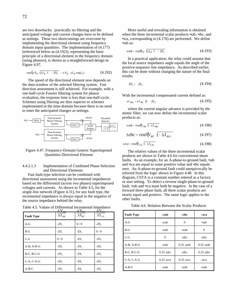
72
are two drawbacks: practically no filtering and the anticipated voltage and current changes have to be defined as settings. These two shortcomings are overcome by implementing the directional element using frequency domain input quantities. The implementation of (4.177) (referenced below as (4.192)), representing the basic principle of a directional element in the frequency domain (using phasors), is shown as a straightforward design in Figure 4.97.
( )( ) )cos(1 1 θRRRR IVZSIVreal ∆⋅∆=−∠⋅∆⋅∆ (4.192)
The speed of the directional element now depends on the data-window of the selected filtering system. Fast direction assessment is still achieved. For example, with a one-half-cycle Fourier filtering system for phasor evaluation, the response time is less than one-half-cycle. Schemes using filtering are then superior to schemes implemented in the time-domain because there is no need to enter the anticipated changes as settings.
Delay T
ir(t)ThresholdDetector
vr(t)
−∆Irc(t)Time-invariantPhasor Filtering
System
Time-invariantPhasor Filtering
SystemDelay T ∆Vr(t)
ScalarProduct
Mimic
Figure 4.47. Frequency-Domain Generic Superimposed Quantities Directional Element
4.4.2.1.3 Implementation of Combined Phase-Selection and Directional Elements
Fast fault-type selection can be combined with directional assessment using the incremental impedances based on the differential (across two phases) superimposed voltages and currents. As shown in Table 4.5, for the single-line network (Figure 4.31), for any fault type, the incremental impedance is always equal to the negative of the source impedance behind the relay.
Table 4.5. Values of Differential Incremental Impedance
Fault Type
∆ VAB
∆ IAB
∆ VBC
∆ IBC
∆ VCA
∆ ICA
A-G -ZS1 0 / 0 -ZS1
B-G -ZS1 -ZS1 0 / 0
C-G 0 / 0 -ZS1 -ZS1
A-B, A-B-G -ZS1 -ZS1 -ZS1
B-C, B-C-G -ZS1 -ZS1 -ZS1
C-A, C-A-G -ZS1 -ZS1 -ZS1
A-B-C -ZS1 -ZS1 -ZS1
More useful and revealing information is obtained when the three incremental scalar products •tab, •tbc, and •tca, corresponding to (4.176) are performed. We define •tab as:
( )( )11 ZSIVrealtab RR −∠⋅∆⋅=∆ (4.193)
In a practical application, the relay could assume that the local source impedance angle equals the angle of the positive-sequence line impedance. As described earlier, this can be done without changing the nature of the final results.
11 ZLZS ∠=∠ (4.194)
With the incremental compensated current defined as:
( )11 ZLII ABABc ∠⋅⋅∆=∆ (4.195)
where the current angular advance is provided by the mimic filter, we can now define the incremental scalar products as:
( )( )ABcAB IVrealtab ∆−⋅=∆ (4.196)
( )( )BCcBC IVrealtbc ∆−⋅=∆ (4.197)
( )( )CAcCA IVrealtca ∆−⋅=∆ (4.198)
The relative values of the three incremental scalar products are shown in Table 4.6 for conventional shunt faults. As an example, for an A-phase-to-ground fault, •tab and •tca are equal to some positive value and •tbc equals zero. An A-phase-to-ground fault could unequivocally be inferred from the logic shown in Figure 4.48. In this diagram, CSTA is a constant number entered as a factory or user setting. To detect a reverse single-phase-to-ground fault, •tab and •tca must both be negative. In the case of a forward three-phase fault, all three scalar products are nearly equal and positive. The same logic applies to the other faults.
Table 4.6. Relation Between the Scalar Products
Fault Type ∆tab ∆tbc ∆tca
A-G ∆tab 0 •tab
B-G ∆tab ∆tab 0
C-G 0 ∆tbc ∆tbc
A-B, A-B-G ∆tab 0.25 ∆tab 0.25 ∆tab
B-C, B-C-G 0.25 ∆tbc ∆tbc 0.25 ∆tbc
C-A, C-A-G 0.25 ∆tca 0.25 ∆tca ∆tca
A-B-C ∆tab ∆tab ∆tab
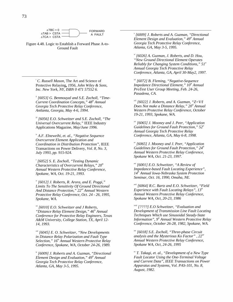
73
FORWARDA FAULT
∆TBC = 0∆TAB > CSTA∆TCA > CSTA
Figure 4.48. Logic to Establish a Forward Phase A-to-Ground Fault
i C. Russell Mason, The Art and Science of Protective Relaying, 1956, John Wiley & Sons, Inc. New York, NY, ISBN 0 471 57552 6. ii [6053] G. Benmouyal and S.E. Zocholl, “Time-Current Coordination Concepts,” 48th Annual Georgia Tech Protective Relay Conference, Antlanta, Georgia, May 4-6, 1994. iii [6056] E.O. Schweitzer and S.E. Zocholl, “The Universal Overcurrent Relay,” IEEE Industry Applications Magazine, May/June 1996. iv A.F. Elneweihi, et. al., “Negative Sequence Overcurrent Element Application and Coordination in Distribution Protection”, IEEE Transactions on Power Delivery, Vol. 8, No. 3, July 1993, pp. 915-924. v [6052] S. E. Zocholl, “Testing Dynamic Characteristics of Overcurrent Relays,” 20th Annual Western Protective Relay Conference, Spokane, WA, Oct. 19-21, 1993. vi [6012] J. Roberts, R. Arora, and E. Poggi,” Limits To The Sensitivity Of Ground Directional And Distance Protection,” 22nd Annual Western Protective Relay Conference, Oct. 24 - 26, 1995, Spokane, WA. vii [6010] E.O. Schweitzer and J Roberts, “Distance Relay Element Design,” 46th Annual Conference for Protective Relay Engineers, Texas A&M University, College Station, TX, April 12-14, 1993. viii [6045] E. O. Schweitzer, “New Developments in Distance Relay Polarization and Fault Type Selection,” 16th Annual Western Protective Relay Conference, Spokane, WA, October 24-26, 1989. ix [6009] J. Roberts and A. Guzman, “Directional Element Design and Evaluation,” 49th Annual Georgia Tech Protective Relay Conference, Atlanta, GA, May 3-5, 1995.
x [6009] J. Roberts and A. Guzman, “Directional Element Design and Evaluation,” 49th Annual Georgia Tech Protective Relay Conference, Atlanta, GA, May 3-5, 1995. xi [6026] A. Guzman, J. Roberts, and D. Hou, “New Ground Directional Element Operates Reliably for Changing System Conditions,” 51st Annual Georgia Tech Protective Relay Conference, Atlanta, GA, April 30-May2, 1997. xii [6072] B. Fleming, “Negative-Sequence Impedance Directional Element,” 10th Annual ProTest User Group Meeting, Feb. 24-26, Pasadena, CA. xiii [6022] J. Roberts, and A. Guzman, “Z=V/I Does Not make a Distance Relay,” 20th Annual Western Protective Relay Conference, October 19-21, 1993, Spokane, WA. xiv [6065] J. Mooney and J. Peer, “Application Guidelines for Ground Fault Protection,” 52st Annual Georgia Tech Protective Relay Conference, Atlanta, GA, May 6-8, 1998. xv [6065] J. Mooney and J. Peer, “Application Guidelines for Ground Fault Protection,” 24th Annual Western Protective Relay Conference, Spokane WA, Oct. 21-23, 1997. xvi [6001] E.O. Schweitzer, “A Review of Impedance-based Fault Locating Experience”, 14th Annual Iowa-Nebraska System Protection Seminar, Oct. 16, 1990, Omaha, NE. xvii [6064] R.C. Bartz and E.O. Schweitzer, “Field Experience with Fault Locating Relays”, 13th Annual Western Protective Relay Conference, Spokane WA, Oct, 20-23, 1986 xviii [????] E.O Schweitzer, “Evaluation and Development of Transmission Line Fault Locating Techniques Which use Sinusoidal Steady-State Information”, 9th Annual Western Protective Relay Conference, October 26-28, 1982, Spokane, WA. xix [6018] S.E. Zocholl, “Three-phase Circuit analysis and the Mysterious Ko Factor” , 22nd Annual Western Protective Relay Conference, Spokane WA, Oct, 24-26, 1995 xx T. Takagi, et. al., “Development of a New Type Fault Locator Using the One-Terminal Voltage and Current Data”, IEEE Transactions on Power Apparatus and Systems, Vol. PAS-101, No. 8, August, 1982.
74
xxi D Novosel, et. al. “Unsynchronized Two-terminal Fault Location Estimate”, IEEE Transactions on Power Delivery, Vol. 7, No. 1, Jan. 1992, pp. 98-107 xxiii G. Benmouyal and J. Roberts, “Superimposed Quantities: Their True Nature and Application in Relays”, Western Protective Relay Conference, Oct. 1999, Spokane WA.
xxiv V. Cook, Analysis of Distance Protection, Research Study Press Ltd., John Wiley & Sons
Inc, 1985.

11. 7 APPENDIX VII. NETWORK THEORY - METHODS FOR GENERATING A SIMPLE FAULT STUDY USING MATHCAD
11.7.1 Introduction
The understanding of relay operations begins with a thorough knowledge of the power system it is designed to protect. Before the days of personal computers and engineering mathematics programs such as Matlab, Mathcad, Solver Q engineers relied on “back of the envelope” calculations to provide ballpark estimates. These estimates are important to verify that data is being used properly in more complex and detailed programs for calculating system load flow and fault studies. The following discussion describes the process of generating a simple Mathcad program to analyze faults on the two-source system shown in Figure Error! No text of specified style in document..1.
The general approach for modeling an electrical network is to first build an admittance matrix representing the branches between nodes in the system. Next, dividing the voltage sources by the respective source impedance generates a current vector. The inverse of the admittance matrix is multiplied times the current vector to compute all the node voltages. Individual branch currents are then computed as the voltage difference between two nodes divided by the impedance between them.
The reason the computer is handy is that the programs are extremely efficient when trying to solve a large number of simultaneous equations. Even for the simple system shown in Figure Error! No text of specified style in document..1, 12 simultaneous equations must be solved to compute the four three-phase nodes. Inverting a matrix larger than three by three should only be done once in any ones lifetime.
In the process that follows, note that only node increase the size of the system matrix and additional branches between existing nodes to not. Consequently, a parallel line between nodes two and four can be simply added as well as additional loads at any existing bus.
11.7.2 System Considerations and the Single line diagram
The single line diagram is critical to knowing where the desired mathematical reside in the solution vectors. The order that data is entered into the current vector and admittance matrix is completely arbitrary but consistency is required. For the system considered here, we have chosen to number the nodes from right to left simply for convenience. For the system shown in Figure Error! No text of specified style in document..1 eventually, the 12 simultaneous equations shown in Figure Error! No text of specified style in document..2 will need to be solved. Fortunately for us today, the engineering programs previously mentioned handle matrices and vectors with almost the same degree of ease as scalar mathematics. If the admittance for each node is grouped as a 3 by 3 matrix, then the mathematics can be viewed as the four by four matrix shown in Figure Error! No text of specified style in document..3. The engineering program still must solve all 12 equations shown in Figure Error! No text of specified style in document..2. The methodologies for generating the three by three matrices and grouping them to form the 12 by 12 matrix will be presented in the following sections.
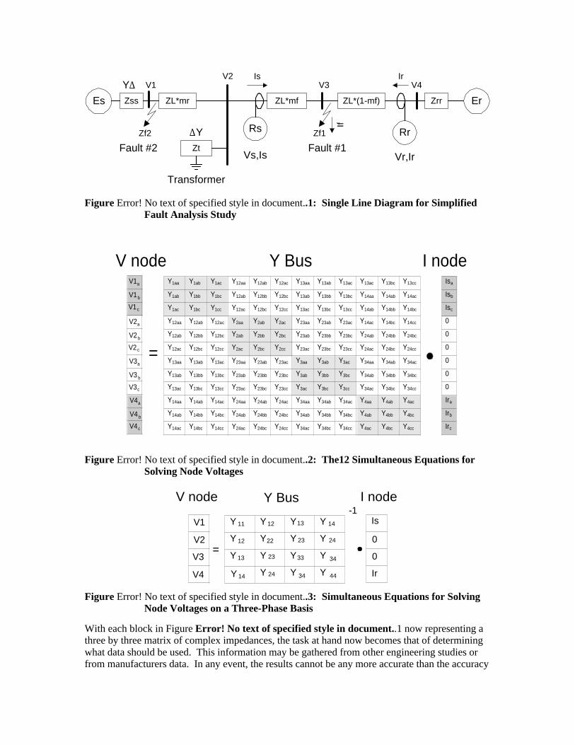
Rs Rr
ZL*mf ZL*(1-mf) Zrr
Vs,Is Vr,Ir
Is Ir
Zf1
Er
V2V3 V4
Zss ZL*mr
Zf2
Es
V1
Zt
Y∆
∆Y
Transformer
If
Fault #1Fault #2
Figure Error! No text of specified style in document..1: Single Line Diagram for Simplified Fault Analysis Study
Y Bus I nodeIsa
Isb
Isc
0
0
0
0
0
0
Ira
Irb
Irc
Y1aa Y1ab Y1ac Y12aa Y12ab Y12ac Y13aa Y13ab Y13ac Y13ac Y13bc Y13cc
Y1ab Y1bb Y1bc Y12ab Y12bb Y12bc Y13ab Y13bb Y13bc Y14aa Y14ab Y14ac
Y1ac Y1bc Y1cc Y12ac Y12bc Y12cc Y13ac Y13bc Y13cc Y14ab Y14bb Y14bc
Y12aa Y12ab Y12ac Y2aa Y2ab Y2ac Y23aa Y23ab Y23ac Y14ac Y14bc Y14cc
Y12ab Y12bb Y12bc Y2ab Y2bb Y2bc Y23ab Y23bb Y23bc Y24ab Y24bb Y24bc
Y12ac Y12bc Y12cc Y2ac Y2bc Y2cc Y23ac Y23bc Y23cc Y24ac Y24bc Y24cc
Y13aa Y13ab Y13ac Y23aa Y23ab Y23ac Y3aa Y3ab Y3ac Y34aa Y34ab Y34ac
Y13ab Y13bb Y13bc Y23ab Y23bb Y23bc Y3ab Y3bb Y3bc Y34ab Y34bb Y34bc
Y13ac Y13bc Y13cc Y23ac Y23bc Y23cc Y3ac Y3bc Y3cc Y34ac Y34bc Y34cc
Y14aa Y14ab Y14ac Y24aa Y24ab Y24ac Y34aa Y34ab Y34ac Y4aa Y4ab Y4ac
Y14ab Y14bb Y14bc Y24ab Y24bb Y24bc Y34ab Y34bb Y34bc Y4ab Y4bb Y4bc
Y14ac Y14bc Y14cc Y24ac Y24bc Y24cc Y34ac Y34bc Y34cc Y4ac Y4bc Y4cc
b
c
V1a
V1
V1
b
c
V2a
V2
V2
b
c
V3a
V3
V3
b
c
V4a
V4
V4
=
V node
Figure Error! No text of specified style in document..2: The12 Simultaneous Equations for Solving Node Voltages
I nodeY Bus
Is
Ir
0
0
V1
V4
V2
V3
Y 11 Y Y Y
Y 12 Y Y Y
Y 13 Y Y Y
Y Y YY 14
22
33
44
12 13 14
24
24
23
23
34
34=
V node-1
Figure Error! No text of specified style in document..3: Simultaneous Equations for Solving Node Voltages on a Three-Phase Basis
With each block in Figure Error! No text of specified style in document..1 now representing a three by three matrix of complex impedances, the task at hand now becomes that of determining what data should be used. This information may be gathered from other engineering studies or from manufacturers data. In any event, the results cannot be any more accurate than the accuracy
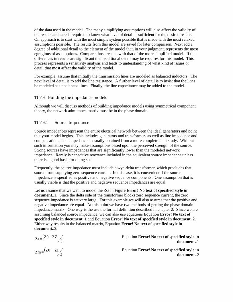
of the data used in the model. The many simplifying assumptions will also affect the validity of the results and care is required to know what level of detail is sufficient for the desired results. On approach is to start with the most simple system possible that is made with the most relaxed assumptions possible. The results from this model are saved for later comparison. Next add a degree of additional detail to the element of the model that, in your judgment, represents the most egregious of assumptions. Compare those results with that of the more simplified model. If the differences in results are significant then additional detail may be requires for this model. This process represents a sensitivity analysis and leads to understanding of what kind of issues or detail that most affect the validity of the model.
For example, assume that initially the transmission lines are modeled as balanced inductors. The next level of detail is to add the line resistance. A further level of detail is to insist that the lines be modeled as unbalanced lines. Finally, the line capacitance may be added to the model.
11.7.3 Building the impedance models
Although we will discuss methods of building impedance models using symmetrical component theory, the network admittance matrix must be in the phase domain.
11.7.3.1 Source Impedance
Source impedances represent the entire electrical network between the ideal generators and point that your model begins. This includes generators and transformers as well as line impedance and compensation. This impedance is usually obtained from a more complete fault study. Without such information you may make assumptions based upon the perceived strength of the source. Strong sources have impedances that are significantly lower than the modeled network impedance. Rarely is capacitive reactance included in the equivalent source impedance unless there is a good basis for doing so.
Frequently, the source impedance must include a wye-delta transformer, which precludes that source from supplying zero sequence current. In this case, it is convenient if the source impedance is specified as positive and negative sequence components. One assumption that is usually viable is that the positive and negative sequence impedances are equal.
Let us assume that we want to model the Zss in Figure Error! No text of specified style in document..1. Since the delta side of the transformer blocks zero sequence current, the zero sequence impedance is set very large. For this example we will also assume that the positive and negative impedance are equal. At this point we have two methods of getting the phase domain impedance matrix. One way is the use the formal definition described in chapter 2. Since we are assuming balanced source impedance, we can also use equations Equation Error! No text of specified style in document..1 and Equation Error! No text of specified style in document..2. Either way results in the balanced matrix, Equation Error! No text of specified style in document..3.
( )3
1Z20ZZs += Equation Error! No text of specified style in document..1
( )3
1Z0ZZm −= Equation Error! No text of specified style in document..2
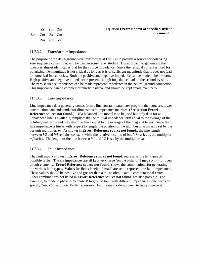
=
ZsZmZm
ZmZsZm
ZmZmZs
Zss
Equation Error! No text of specified style in document..3
11.7.3.2 Transformer Impedance
The purpose of the delta-ground wye transformer at Bus 2 is to provide a source for polarizing zero sequence current that will be used in some relay studies. The approach to generating the matrix is almost identical as that for the source impedance. Since the residual current is used for polarizing the magnitude is not critical as long as it is of sufficient magnitude that it does not lead to numerical inaccuracies. Both the positive and negative impedance can be made to be the same. High positive and negative impedance represents a high impedance load on the secondary side. The zero sequence impedance can be made represent impedance in the neutral ground connection. This impedance can be complex or purely resistive and should be kept small, even zero.
11.7.3.3 Line Impedance
Line impedance data generally comes form a line constant parameter program that converts tower construction data and conductor dimensions to impedance matrices. (See section Error! Reference source not found.). If a balanced line model is to be used but only data for an unbalanced line is available, simply make the mutual impedance term equal to the average of the off-diagonal terms and the self-impedance equal to the average of the diagonal terms. Since the line impedance is linear with respect to length, the position of the fault bus is arbitrarily set by the per unit multiplier, m. As shown in Error! Reference source not found., the line length between V2 and V4 remains constant while the relative location of bus V3 varies as the multiplier mf varies. The length of the line between V1 and V2 is set by the multiplier mr.
11.7.3.4 Fault Impedance
The fault matrix shown in Error! Reference source not found. represents the ten types of possible faults. The six impedances are all kept very large (on the order of 1 mega ohm) for open circuit elements. Error! Reference source not found. shows the combinations for generating the various fault types. Values for fields labeled “small” are set to represent the fault impedance. These values should be positive and greater than a micro ohm to avoid computational errors. Other combinations not listed in Error! Reference source not found. are also possible. For example, to model a phase A to phase B to ground fault with different impedances, one needs to specify Zaa, Zbb, and Zab. Faults represented by this matrix do not need to be symmetrical.
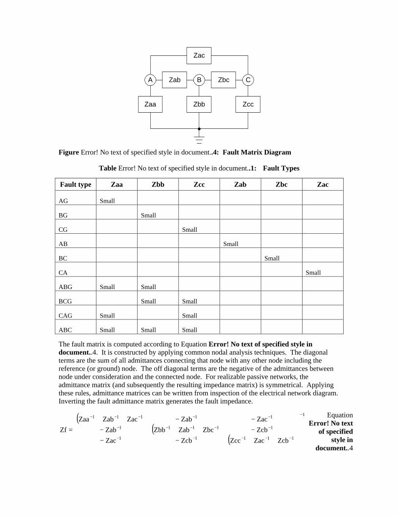
ZabA B CZbc
Zac
Zaa Zbb Zcc
Figure Error! No text of specified style in document..4: Fault Matrix Diagram
Table Error! No text of specified style in document..1: Fault Types
Fault type Zaa Zbb Zcc Zab Zbc Zac
AG Small
BG
Small
CG
Small
AB
Small
BC
Small
CA
Small
ABG Small Small
BCG
Small Small
CAG Small
Small
ABC Small Small Small
The fault matrix is computed according to Equation Error! No text of specified style in document..4. It is constructed by applying common nodal analysis techniques. The diagonal terms are the sum of all admittances connecting that node with any other node including the reference (or ground) node. The off diagonal terms are the negative of the admittances between node under consideration and the connected node. For realizable passive networks, the admittance matrix (and subsequently the resulting impedance matrix) is symmetrical. Applying these rules, admittance matrices can be written from inspection of the electrical network diagram. Inverting the fault admittance matrix generates the fault impedance.
( )( )
( )
1
11111
11111
11111
ZcbZacZccZcbZac
ZcbZbcZabZbbZab
ZacZabZacZabZaa
Zf
−
−−−−−
−−−−−
−−−−−
++−−−++−−−++
=
Equation Error! No text
of specified style in
document..4
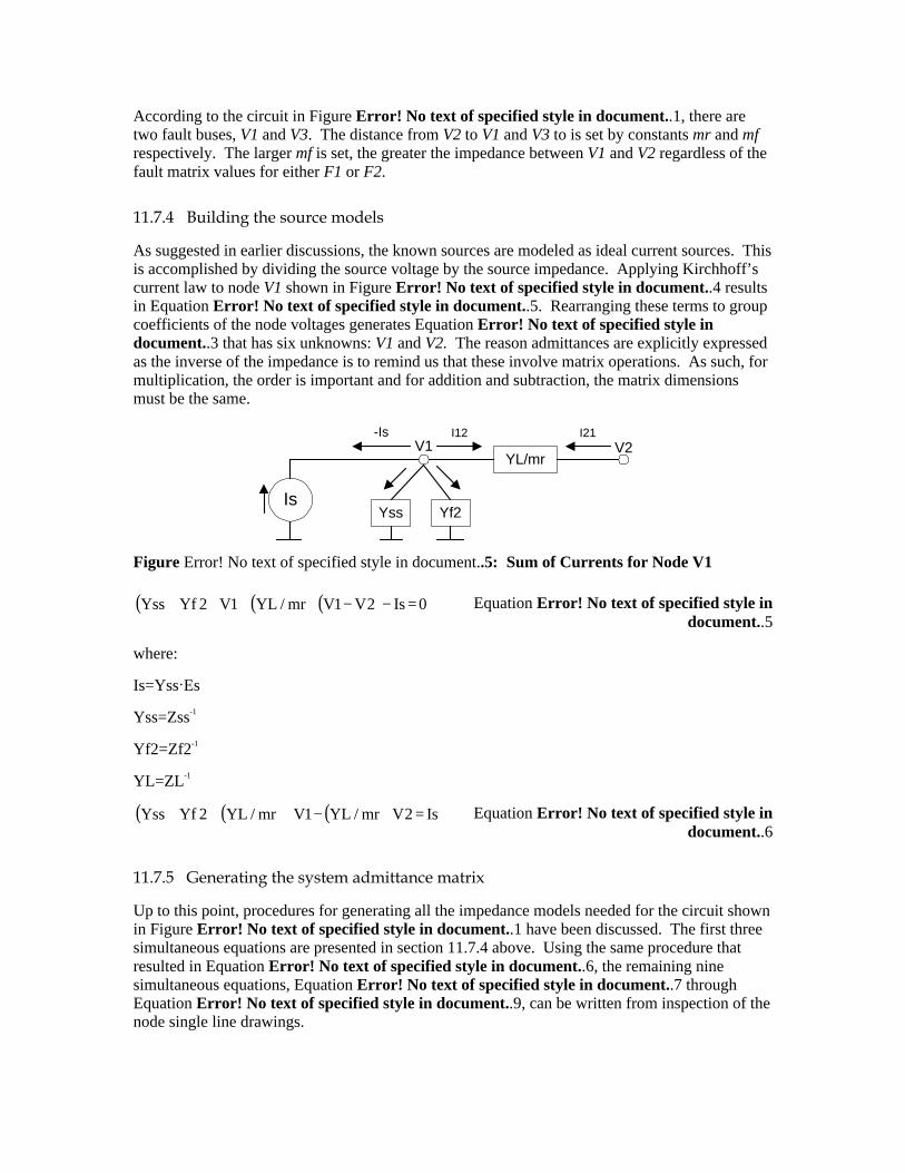
According to the circuit in Figure Error! No text of specified style in document..1, there are two fault buses, V1 and V3. The distance from V2 to V1 and V3 to is set by constants mr and mf respectively. The larger mf is set, the greater the impedance between V1 and V2 regardless of the fault matrix values for either F1 or F2.
11.7.4 Building the source models
As suggested in earlier discussions, the known sources are modeled as ideal current sources. This is accomplished by dividing the source voltage by the source impedance. Applying Kirchhoff’s current law to node V1 shown in Figure Error! No text of specified style in document..4 results in Equation Error! No text of specified style in document..5. Rearranging these terms to group coefficients of the node voltages generates Equation Error! No text of specified style in document..3 that has six unknowns: V1 and V2. The reason admittances are explicitly expressed as the inverse of the impedance is to remind us that these involve matrix operations. As such, for multiplication, the order is important and for addition and subtraction, the matrix dimensions must be the same.
Yss
YL/mr
Is
V1
Yf2
V2-Is I21I12
Figure Error! No text of specified style in document..5: Sum of Currents for Node V1
( ) ( ) ( ) 0Is2V1Vmr/YL1V2YfYss =−−⋅+⋅+ Equation Error! No text of specified style in document..5
where:
Is=Yss«Es
Yss=Zss-1
Yf2=Zf2-1
YL=ZL-1
( )( ) ( ) Is2Vmr/YL1Vmr/YL2YfYss =⋅−⋅++ Equation Error! No text of specified style in document..6
11.7.5 Generating the system admittance matrix
Up to this point, procedures for generating all the impedance models needed for the circuit shown in Figure Error! No text of specified style in document..1 have been discussed. The first three simultaneous equations are presented in section 11.7.4 above. Using the same procedure that resulted in Equation Error! No text of specified style in document..6, the remaining nine simultaneous equations, Equation Error! No text of specified style in document..7 through Equation Error! No text of specified style in document..9, can be written from inspection of the node single line drawings.
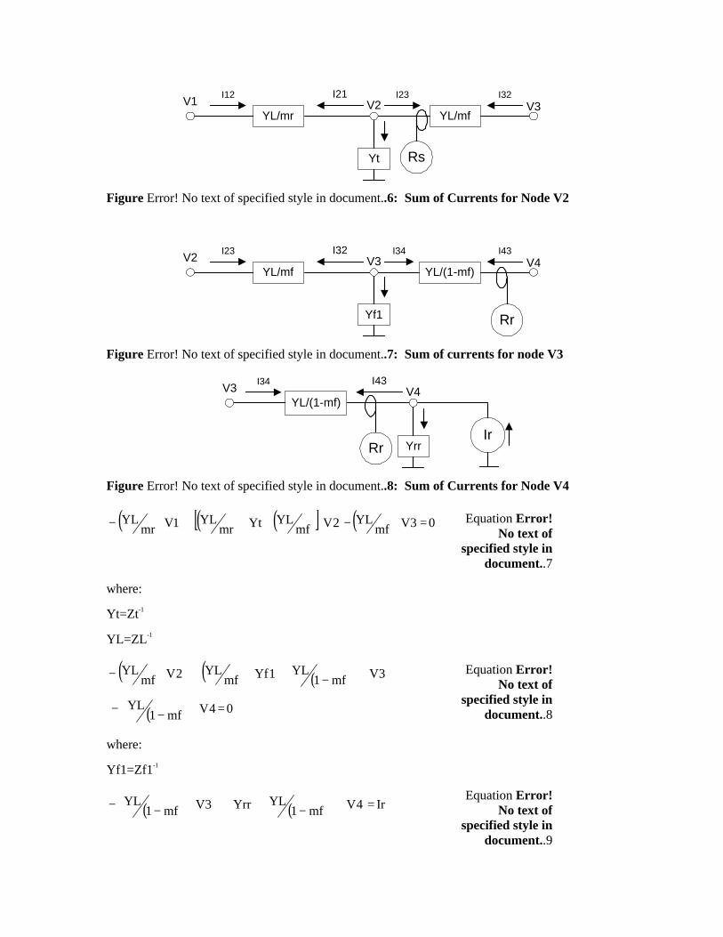
Rs
YL/mfV2
Yt
V3I21 I32I23
YL/mrV1
I12
Figure Error! No text of specified style in document..6: Sum of Currents for Node V2
Rr
YL/(1-mf)V3
Yf1
V4I32 I43I34
YL/mfV2
I23
Figure Error! No text of specified style in document..7: Sum of currents for node V3
Rr
V4I43
YL/(1-mf)V3
I34
IrYrr
Figure Error! No text of specified style in document..8: Sum of Currents for Node V4
( ) ( ) ( )[ ] ( ) 03VmfYL2Vmf
YLYtmrYL1Vmr
YL =⋅−⋅+++⋅− Equation Error! No text of
specified style in document..7
where:
Yt=Zt-1
YL=ZL-1
( ) ( ) ( )
( ) 04Vmf1YL
3Vmf1YL1Yfmf
YL2VmfYL
=⋅
−−
⋅
−+++⋅−
Equation Error! No text of
specified style in document..8
where:
Yf1=Zf1-1
( ) ( ) Ir4Vmf1YLYrr3Vmf1
YL =⋅
−++⋅
−− Equation Error!
No text of specified style in
document..9
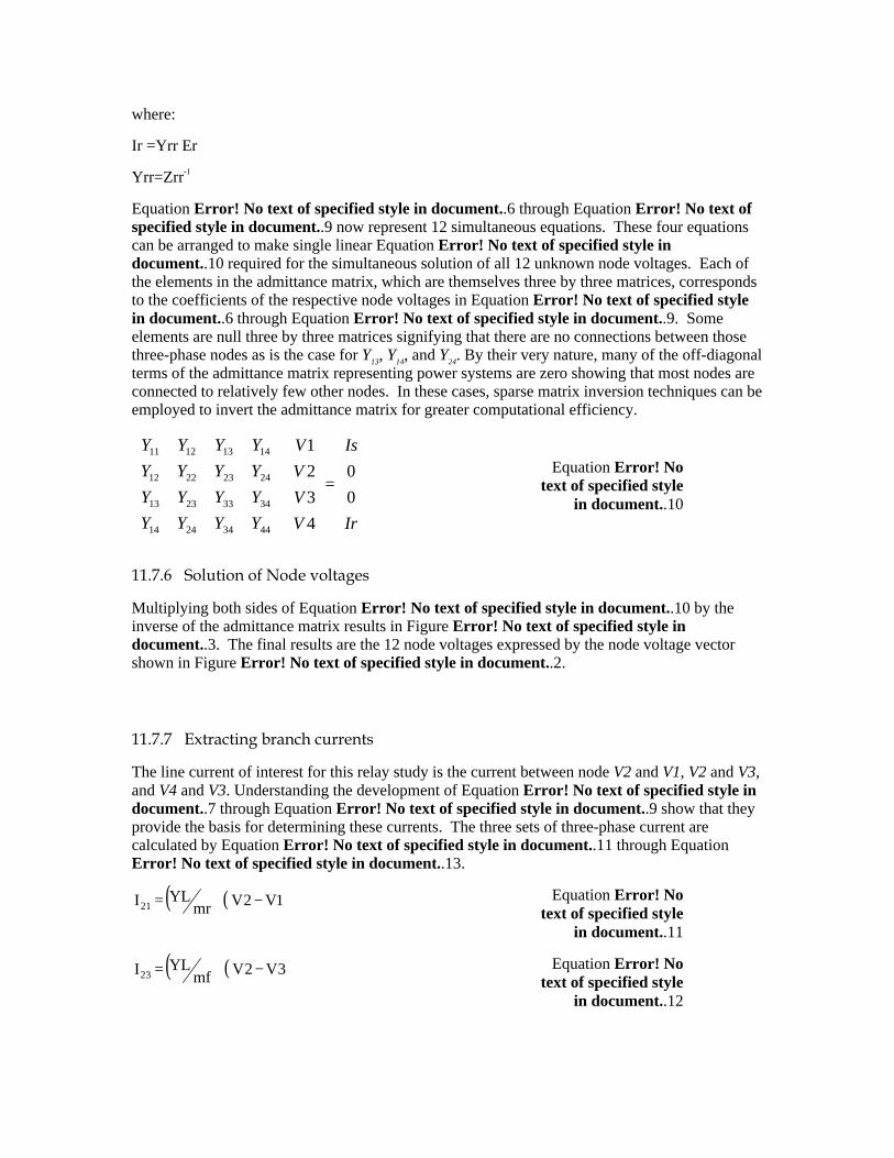
where:
Ir =Yrr⋅Er
Yrr=Zrr-1
Equation Error! No text of specified style in document..6 through Equation Error! No text of specified style in document..9 now represent 12 simultaneous equations. These four equations can be arranged to make single linear Equation Error! No text of specified style in document..10 required for the simultaneous solution of all 12 unknown node voltages. Each of the elements in the admittance matrix, which are themselves three by three matrices, corresponds to the coefficients of the respective node voltages in Equation Error! No text of specified style in document..6 through Equation Error! No text of specified style in document..9. Some elements are null three by three matrices signifying that there are no connections between those three-phase nodes as is the case for Y13, Y14, and Y24. By their very nature, many of the off-diagonal terms of the admittance matrix representing power systems are zero showing that most nodes are connected to relatively few other nodes. In these cases, sparse matrix inversion techniques can be employed to invert the admittance matrix for greater computational efficiency.
=
⋅
Ir
Is
V
V
V
V
YYYY
YYYY
YYYY
YYYY
0
0
4
3
2
1
44342414
34332313
24232212
14131211
Equation Error! No
text of specified style in document..10
11.7.6 Solution of Node voltages
Multiplying both sides of Equation Error! No text of specified style in document..10 by the inverse of the admittance matrix results in Figure Error! No text of specified style in document..3. The final results are the 12 node voltages expressed by the node voltage vector shown in Figure Error! No text of specified style in document..2.
11.7.7 Extracting branch currents
The line current of interest for this relay study is the current between node V2 and V1, V2 and V3, and V4 and V3. Understanding the development of Equation Error! No text of specified style in document..7 through Equation Error! No text of specified style in document..9 show that they provide the basis for determining these currents. The three sets of three-phase current are calculated by Equation Error! No text of specified style in document..11 through Equation Error! No text of specified style in document..13.
( ) ( )1V2VmrYLI21 −⋅= Equation Error! No
text of specified style in document..11
( ) ( )3V2VmfYLI23 −⋅= Equation Error! No
text of specified style in document..12
( ) ( )3V4Vmf1YLI43 −⋅
−= Equation Error! No
text of specified style in document..13
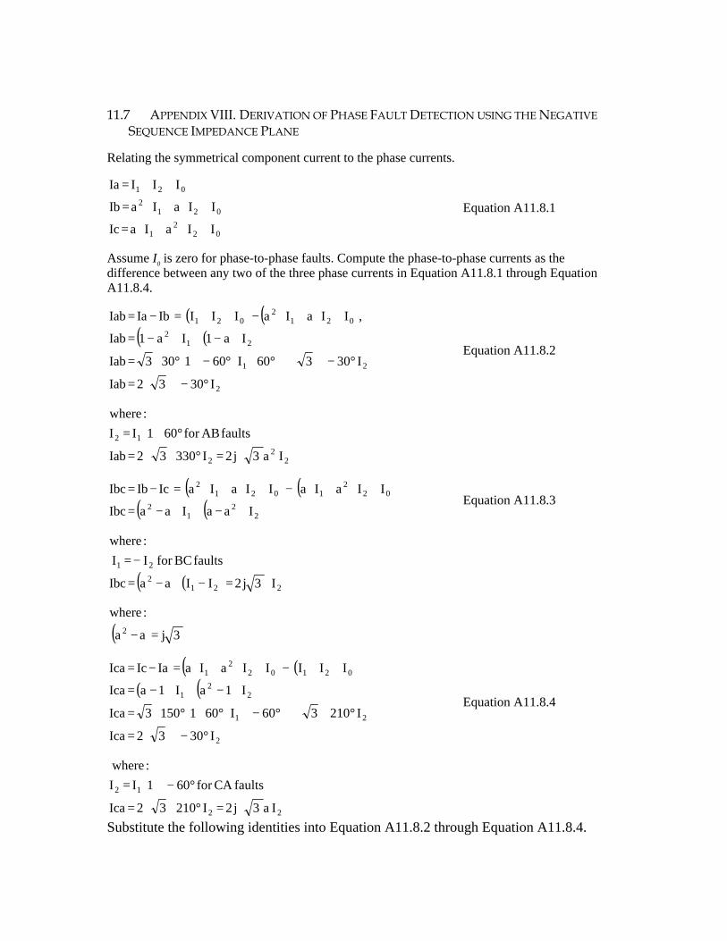
11.7 APPENDIX VIII. DERIVATION OF PHASE FAULT DETECTION USING THE NEGATIVE SEQUENCE IMPEDANCE PLANE
Relating the symmetrical component current to the phase currents.
022
1
0212
021
IIaIaIc
IIaIaIb
IIIIa
+⋅+⋅=
+⋅+⋅=
++=
Equation A11.8.1
Assume I0 is zero for phase-to-phase faults. Compute the phase-to-phase currents as the difference between any two of the three phase currents in Equation A11.8.1 through Equation A11.8.4.
( ) ( )( ) ( )
2
21
212
0212
021
I3032Iab
I30360I601303Iab
Ia1Ia1Iab
,IIaIaIIIIbIaIab
°−∠⋅=
°−∠+°∠⋅°−∠⋅°∠=
⋅−+⋅−=
+⋅+⋅−++=−=
Equation A11.8.2
22
2
12
Ia3j2I33032Iab
faultsABfor601II
:where
⋅⋅=°∠⋅=
°∠⋅=
( ) ( )( ) ( ) 2
21
2
022
10212
IaaIaaIbc
IIaIaIIaIaIcIbIbc
⋅−+⋅−=
+⋅+⋅−+⋅+⋅=−= Equation A11.8.3
( ) ( ) 2212
21
I3j2IIaaIbc
faultsBCforII
:where
⋅=−⋅−=
−=
( ) 3jaa
:where2 =−
( ) ( )( ) ( )
2
21
22
1
021022
1
I3032Ica
I210360I6011503Ica
I1aI1aIca
IIIIIaIaIaIcIca
°−∠⋅=
°∠+°−∠⋅°∠⋅°∠=
⋅−+⋅−=
++−+⋅+⋅=−=
Equation A11.8.4
22
12
Ia3j2I21032Ica
faultsCAfor601II
:where
⋅⋅=°∠⋅=
°−∠⋅=
Substitute the following identities into Equation A11.8.2 through Equation A11.8.4.
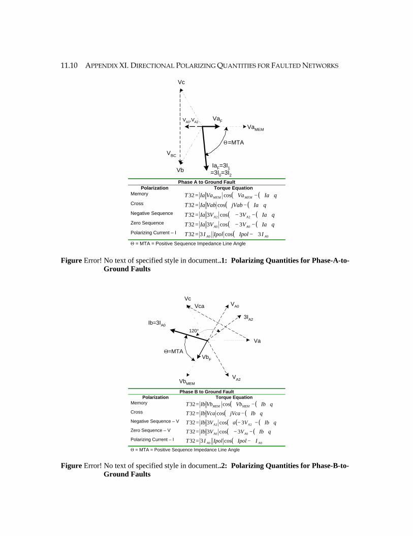
11.10 APPENDIX XI. DIRECTIONAL POLARIZING QUANTITIES FOR FAULTED NETWORKS
Vc
VA0,VA2
VaMEM
VbIaF=3I1=3I0=3I2
Θ=MTA
VaF
VBC
Phase A to Ground Fault Polarization Torque Equation
Memory ( )( )θ+∠−∠= IaVaVaIaT MEMMEM cos32
Cross ( )( )θ+∠−∠= IajVabVabIaT cos32
Negative Sequence ( )( )θ+∠−−∠= IaVVIaT AA 22 3cos332
Zero Sequence ( )( )θ+∠−−∠= IaVVIaT AA 00 3cos332
Polarizing Current – I ( )00 3cos332 AA IIpolIpolIT ∠−∠=
Θ = MTA = Positive Sequence Impedance Line Angle
Figure Error! No text of specified style in document..1: Polarizing Quantities for Phase-A-to-Ground Faults
Vc
VA2
Va
VbMEM
Ib=3IA0
Θ=MTA
VA0
3IA2
VbF
Vca
Phase B to Ground Fault Polarization Torque Equation
Memory ( )( )θ+∠−∠= IbVbVbIbT MEMMEM cos32
Cross ( )( )θ+∠−∠= IbjVcaVcaIbT cos32
Negative Sequence – V ( ) ( )( )θ+∠−−∠= IbVaVIbT AA 22 3cos332
Zero Sequence – V ( )( )θ+∠−−∠= IbVVIbT AA 00 3cos332
Polarizing Current – I ( )00 cos332 AA IIpolIpolIT ∠−∠=
Θ = MTA = Positive Sequence Impedance Line Angle
120°
Figure Error! No text of specified style in document..2: Polarizing Quantities for Phase-B-to-Ground Faults
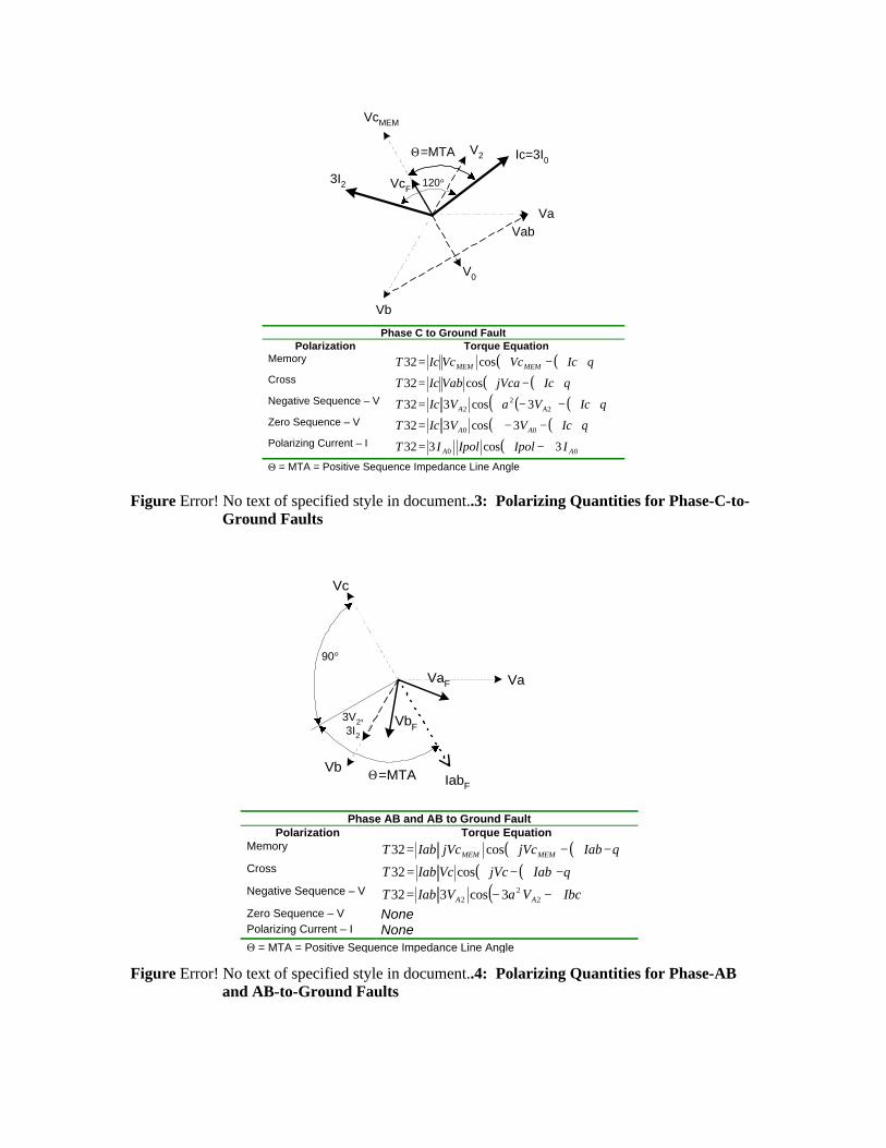
Va
V2
VcMEM
Vb
Ic=3I0Θ=MTA
V0
3I2 120° VcF
Vab
Phase C to Ground Fault Polarization Torque Equation
Memory ( )( )θ+∠−∠= IcVcVcIcT MEMMEM cos32
Cross ( )( )θ+∠−∠= IcjVcaVabIcT cos32
Negative Sequence – V ( ) ( )( )θ+∠−−∠= IcVaVIcT AA 22
2 3cos332
Zero Sequence – V ( )( )θ+∠−−∠= IcVVIcT AA 00 3cos332
Polarizing Current – I ( )00 3cos332 AA IIpolIpolIT ∠−∠=
Θ = MTA = Positive Sequence Impedance Line Angle
Figure Error! No text of specified style in document..3: Polarizing Quantities for Phase-C-to-Ground Faults
Phase AB and AB to Ground Fault
Polarization Torque Equation Memory ( )( )θ−∠−∠= IabjVcjVcIabT MEMMEM cos32
Cross ( )( )θ−∠−∠= IabjVcVcIabT cos32
Negative Sequence – V ( )IbcVaVIabT AA ∠−−= 22
2 3cos332
Zero Sequence – V None Polarizing Current – I None Θ = MTA = Positive Sequence Impedance Line Angle
Vc
Va
VbIabF
VaF
VbF3V2,3I2
Θ=MTA
90°
Figure Error! No text of specified style in document..4: Polarizing Quantities for Phase-AB and AB-to-Ground Faults
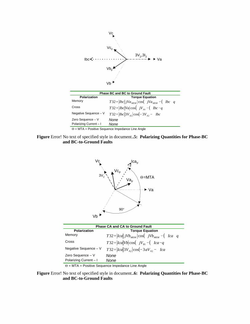
Phase BC and BC to Ground Fault
Polarization Torque Equation Memory ( )( )θ+∠−∠= IbcjVajVaIbcT MEMMEM cos32
Cross ( )( )θ−∠−∠= IbcjVVaIbcT A1cos32
Negative Sequence – V ( )IbcVVIbcT AA ∠−−= 22 3cos332
Zero Sequence – V None Polarizing Current – I None Θ = MTA = Positive Sequence Impedance Line Angle
Vc
Va
Vb
3V2,3I2Ibc
VcF
VbF
Figure Error! No text of specified style in document..5: Polarizing Quantities for Phase-BC and BC-to-Ground Faults
Phase CA and CA to Ground Fault
Polarization Torque Equation Memory ( )( )θ+∠−∠= IcajVbjVbIcaT MEMMEM cos32
Cross ( )( )θ−∠−∠= IcajVVbIcaT B1cos32
Negative Sequence – V ( )IcaaVVIcaT AA ∠−−= 22 3cos332
Zero Sequence – V None Polarizing Current – I None Θ = MTA = Positive Sequence Impedance Line Angle
Vc
Va
Vb
IcaF
VaF
VcF3V2 Θ=MTA
90°
Figure Error! No text of specified style in document..6: Polarizing Quantities for Phase-BC and BC-to-Ground Faults
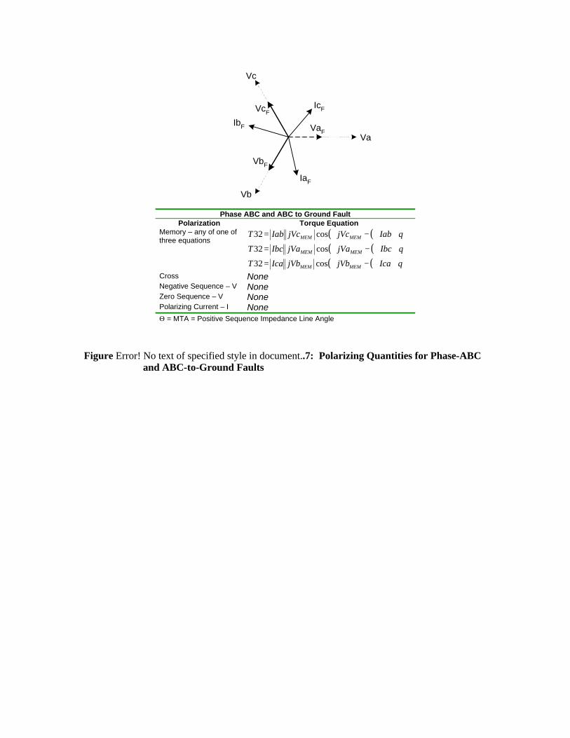
Phase ABC and ABC to Ground Fault
Polarization Torque Equation Memory – any of one of three equations
( )( )θ+∠−∠= IabjVcjVcIabT MEMMEM cos32
( )( )θ+∠−∠= IbcjVajVaIbcT MEMMEM cos32
( )( )θ+∠−∠= IcajVbjVbIcaT MEMMEM cos32
Cross None Negative Sequence – V None Zero Sequence – V None Polarizing Current – I None Θ = MTA = Positive Sequence Impedance Line Angle
Vc
Va
Vb
VcF
VbF
VaF
IaF
IbF
IcF
Figure Error! No text of specified style in document..7: Polarizing Quantities for Phase-ABC and ABC-to-Ground Faults
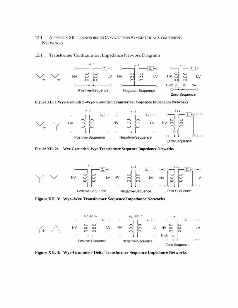
12.1 APPENDIX XII. TRANSFORMER CONNECTION SYMMETRICAL COMPONENT NETWORKS
12.1 Transformer Configuration Impedance Network Diagrams
ZT
LVHV
Positive-Sequence
a : 1
HV
ZT
a : 1
LV
Negative-Sequence
ZT
LV
Zero-Sequence
3ZG
HV
a : 1
3ZGHigh Low
Figure XII. 1 Wye-Grounded.–Wye-Grounded Transformer Sequence Impedance Networks
ZT
HV
Positive-Sequence
a : 1
HV
ZT
a : 1
LV
Negative-Sequence
ZT
a : 1
Zero-Sequence
3ZG
HV
Figure XII. 2: Wye Grounded–Wye Transformer Sequence Impedance Networks
ZT
LV
Zero-Sequence
HV
a : 1ZT
LVHV
Positive-Sequence
a : 1
HV
ZT
a : 1
LV
Negative-Sequence
Figure XII. 3: Wye–Wye Transformer Sequence Impedance Networks
ZT
30o : 1a
LVHV
Positive-Sequence
HV
ZT
-30o : 1a
LV
Negative-Sequence
LV
High
ZT
a : 1
Zero-Sequence
3ZG
HV
Figure XII. 4: Wye-Grounded–Delta Transformer Sequence Impedance Networks
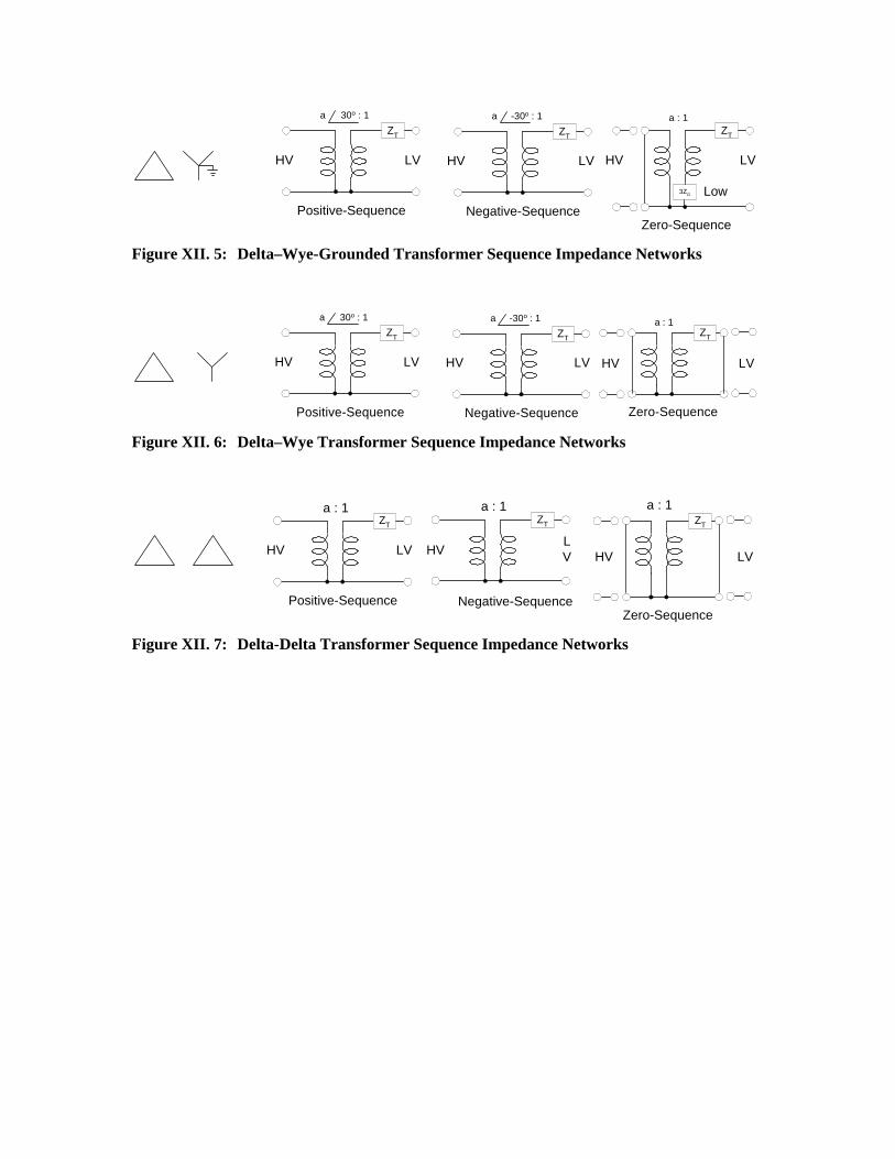
ZT
30o : 1a
LVHV
Positive-Sequence
ZT
-30o : 1a
LVHV
Negative-Sequence
ZT
LV
Zero-Sequence
3ZG Low
HV
a : 1
Figure XII. 5: Delta–Wye-Grounded Transformer Sequence Impedance Networks
ZT
30o : 1a
LVHV
Positive-Sequence
ZT
-30o : 1a
LVHV
Negative-Sequence
ZT
LV
Zero-Sequence
HV
a : 1
Figure XII. 6: Delta–Wye Transformer Sequence Impedance Networks
ZT
LVHV
Positive-Sequence Negative-Sequence
a : 1
HV
ZT
a : 1
LV
ZT
LV
Zero-Sequence
HV
a : 1
Figure XII. 7: Delta-Delta Transformer Sequence Impedance Networks
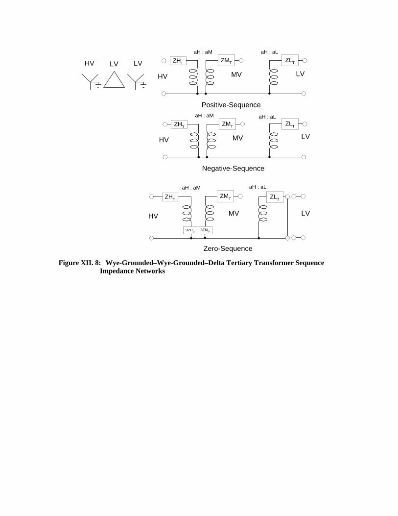
LVHV LV
HV
Positive-Sequence
aH : aM
ZHTZMT
MV LV
ZLT
aH : aL
HV
Negative-Sequence
aH : aM
ZHTZMT
MV LV
ZLT
aH : aL
aH : aM
Zero-Sequence
HV
3ZMG3ZHG
ZHTZMT
MV LV
aH : aL
ZLT
Figure XII. 8: Wye-Grounded–Wye-Grounded–Delta Tertiary Transformer Sequence Impedance Networks
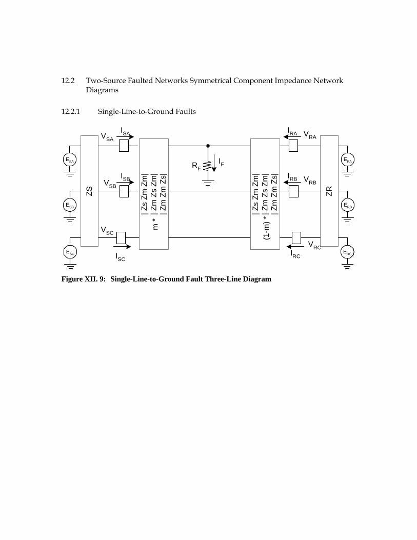
12.2 Two-Source Faulted Networks Symmetrical Component Impedance Network Diagrams
12.2.1 Single-Line-to-Ground Faults
ESB
RF
ISBVSB
ESC
VSC
ERB
IRB VRB
ERC
VRCIRCISC
ESA
ISAVSA
ERA
IRA VRA
IF
ZS
| Zs
Zm
Zm
|| Z
m Z
s Z
m|
| Zm
Zm
Zs|
| Zs
Zm
Zm
|| Z
m Z
s Z
m|
| Zm
Zm
Zs|
m *
(1-m
) *
ZR
Figure XII. 9: Single-Line-to-Ground Fault Three-Line Diagram
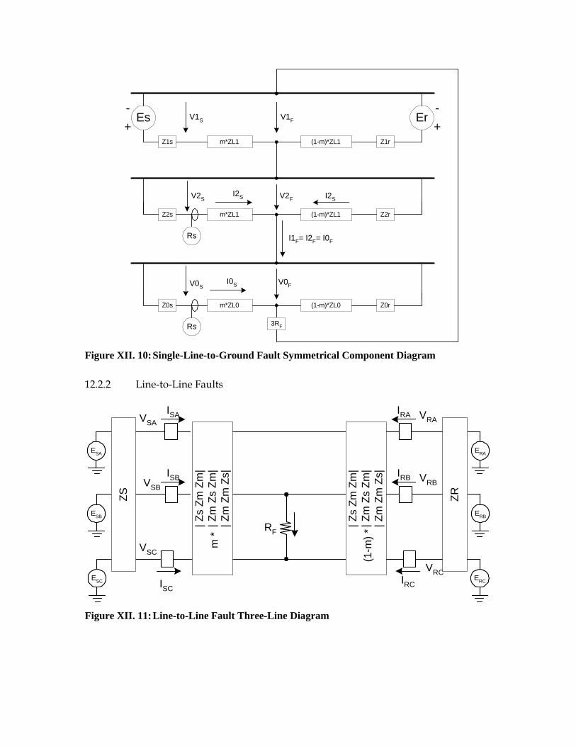
Rs
Rs
Es
Z1s m*ZL1 (1-m)*ZL1 Z1r
Er
Z2s m*ZL1 (1-m)*ZL1 Z2r
Z0s m*ZL0 (1-m)*ZL0 Z0r
3RF
V2FV2S I2SI2S
I1F= I2F= I0F
V0SI0S V0F
+
-
+
-V1S V1F
Figure XII. 10: Single-Line-to-Ground Fault Symmetrical Component Diagram
12.2.2 Line-to-Line Faults
RF
ESB
ISBVSB
ESC
VSC
ERB
IRB VRB
ERC
VRCIRCISC
ESA
ISAVSA
ERA
IRA VRA
ZS
| Zs
Zm
Zm
|| Z
m Z
s Z
m|
| Zm
Zm
Zs|
| Zs
Zm
Zm
|| Z
m Z
s Z
m|
| Zm
Zm
Zs|
m *
(1-m
) *
ZR
Figure XII. 11: Line-to-Line Fault Three-Line Diagram
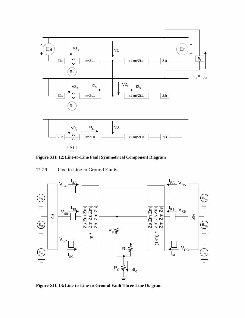
+
-
Rs
Rs
Rs
Es
Z1s m*ZL1 (1-m)*ZL1 Z1r
Er
Z2s m*ZL1 (1-m)*ZL1 Z2r
Z0s m*ZL0 (1-m)*ZL0 Z0r
RF
V2FV2S I2SI2S
IA1 = -IA2
V0SI0S
+
-V1S V1F
V0F
Figure XII. 12: Line-to-Line Fault Symmetrical Component Diagram
12.2.3 Line-to-Line-to-Ground Faults
RF
RG 3I0
RF
ESB
ISBVSB
ESC
VSC
ERB
IRB VRB
ERC
VRCIRCISC
ESA
ISAVSA
ERA
IRA VRA
ZS
| Zs
Zm
Zm
|| Z
m Z
s Z
m|
| Zm
Zm
Zs|
| Zs
Zm
Zm
|| Z
m Z
s Z
m|
| Zm
Zm
Zs|
m *
(1-m
) *
ZR
Figure XII. 13: Line-to-Line-to-Ground Fault Three-Line Diagram
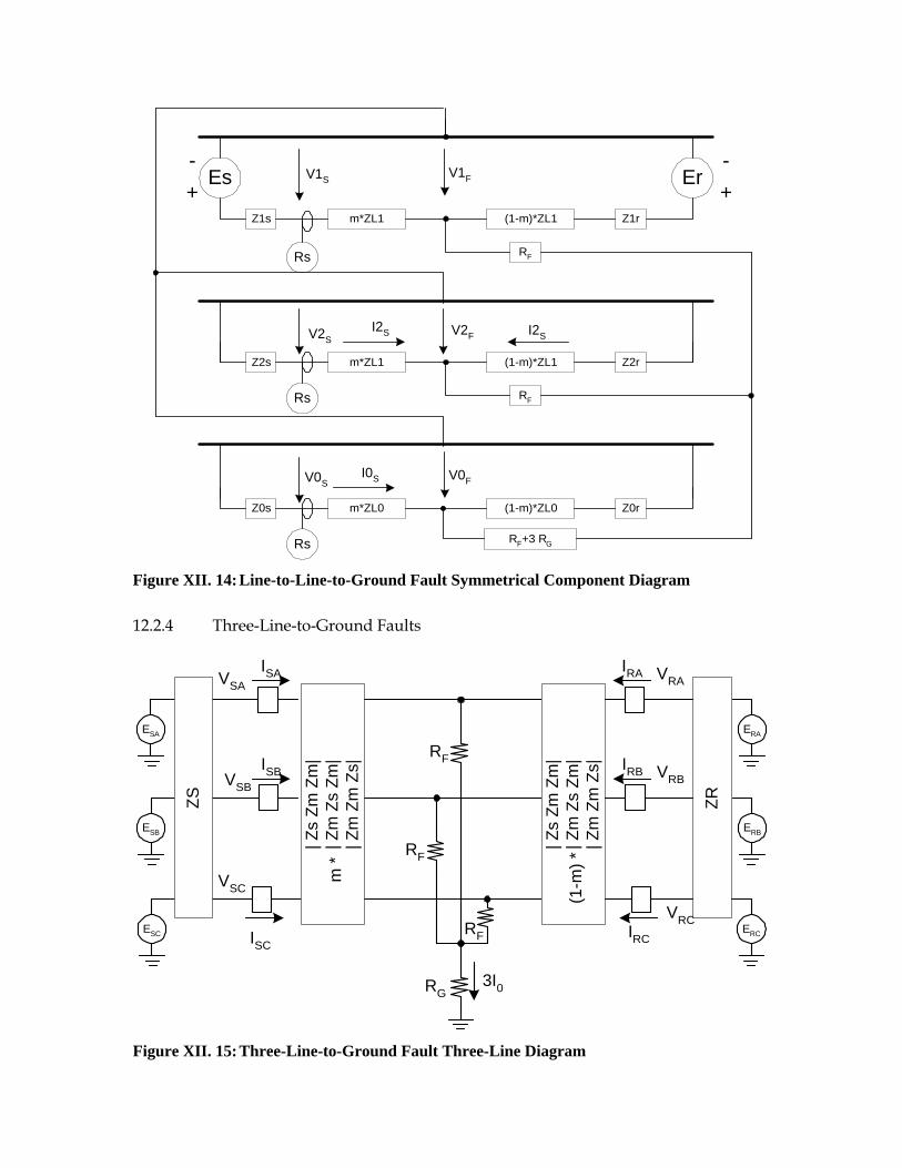
Rs
Rs
Rs
Es
Z1s m*ZL1 (1-m)*ZL1 Z1r
Er
Z2s m*ZL1 (1-m)*ZL1 Z2r
Z0s m*ZL0 (1-m)*ZL0 Z0r
RF
V2FV2SI2S
I2S
V0SI0S
RF
RF+3 RG
+
-
+
-V1S
V1F
V0F
Figure XII. 14: Line-to-Line-to-Ground Fault Symmetrical Component Diagram
12.2.4 Three-Line-to-Ground Faults
RG3I0
RF
RF
RF
ESB
ISBVSB
ESC
VSC
ERB
IRB VRB
ERC
VRCIRCISC
ESA
ISAVSA
ERA
IRA VRA
ZS
| Zs
Zm
Zm
|| Z
m Z
s Z
m|
| Zm
Zm
Zs|
| Zs
Zm
Zm
|| Z
m Z
s Z
m|
| Zm
Zm
Zs|
m *
(1-m
) *
ZR
Figure XII. 15: Three-Line-to-Ground Fault Three-Line Diagram
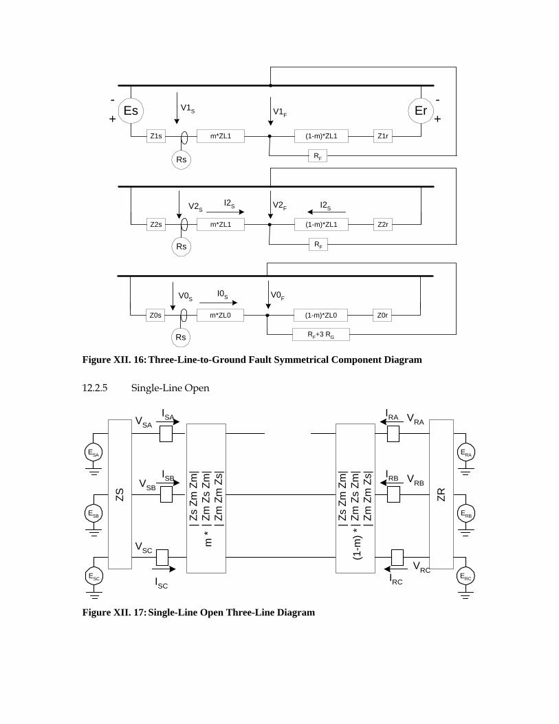
Rs
Rs
Rs
Es
Z1s m*ZL1 (1-m)*ZL1 Z1r
Er
Z2s m*ZL1 (1-m)*ZL1 Z2r
Z0s m*ZL0 (1-m)*ZL0 Z0r
RF
V2FV2SI2S
I2S
V0SI0S
RF
RF+3 RG
+
-
+
-V1S V1F
V0F
Figure XII. 16: Three-Line-to-Ground Fault Symmetrical Component Diagram
12.2.5 Single-Line Open
ESB
ISBVSB
ESC
VSC
ERB
IRB VRB
ERC
VRCIRCISC
ESA
ISAVSA
ERA
IRA VRA
ZS
| Zs
Zm
Zm
|| Z
m Z
s Z
m|
| Zm
Zm
Zs|
| Zs
Zm
Zm
|| Z
m Z
s Z
m|
| Zm
Zm
Zs|
m *
(1-m
) *
ZR
Figure XII. 17: Single-Line Open Three-Line Diagram
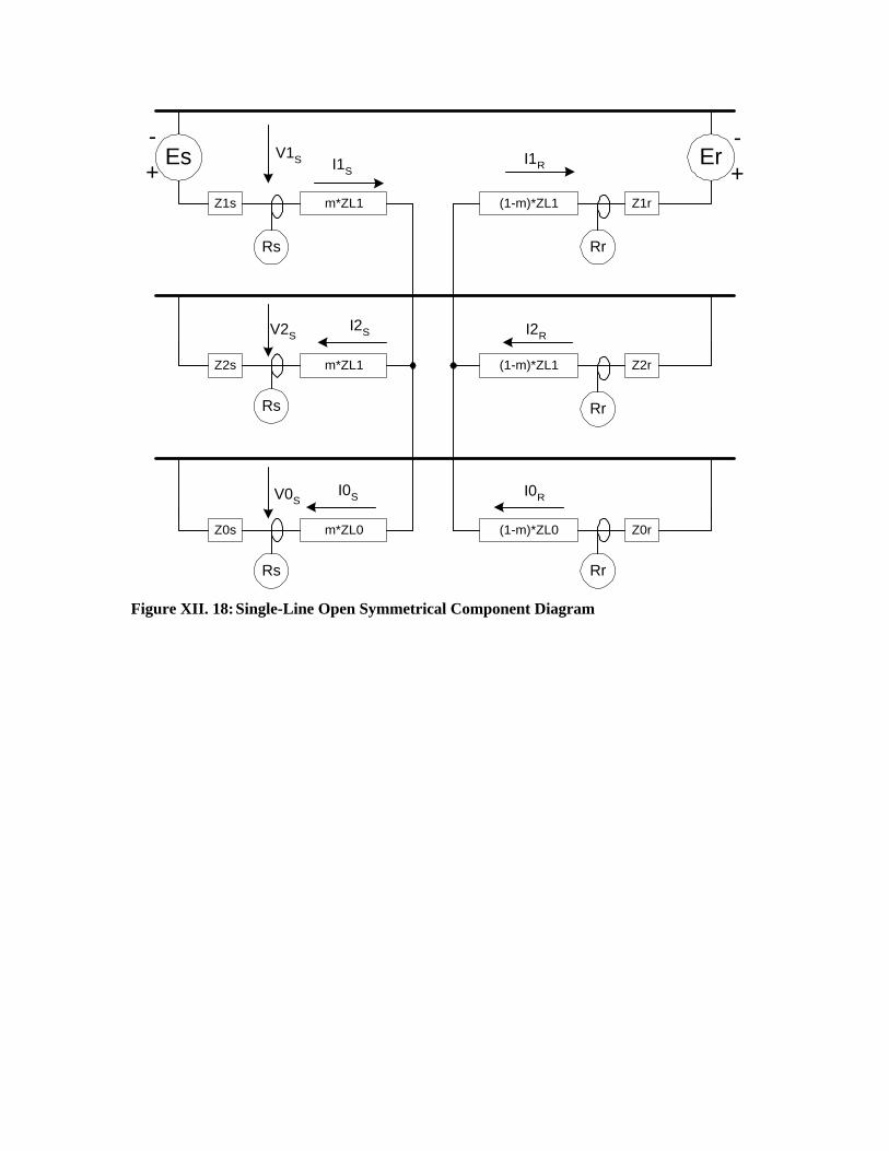
Rr
Rr
RrRs
Rs
Rs
Es
Z1s m*ZL1 (1-m)*ZL1 Z1r
Er
Z2s m*ZL1 (1-m)*ZL1 Z2r
Z0s m*ZL0 (1-m)*ZL0 Z0r
V2S I2RI2S
V0SI0S
+
-
+
-V1S
I0R
I1RI1S
Figure XII. 18: Single-Line Open Symmetrical Component Diagram
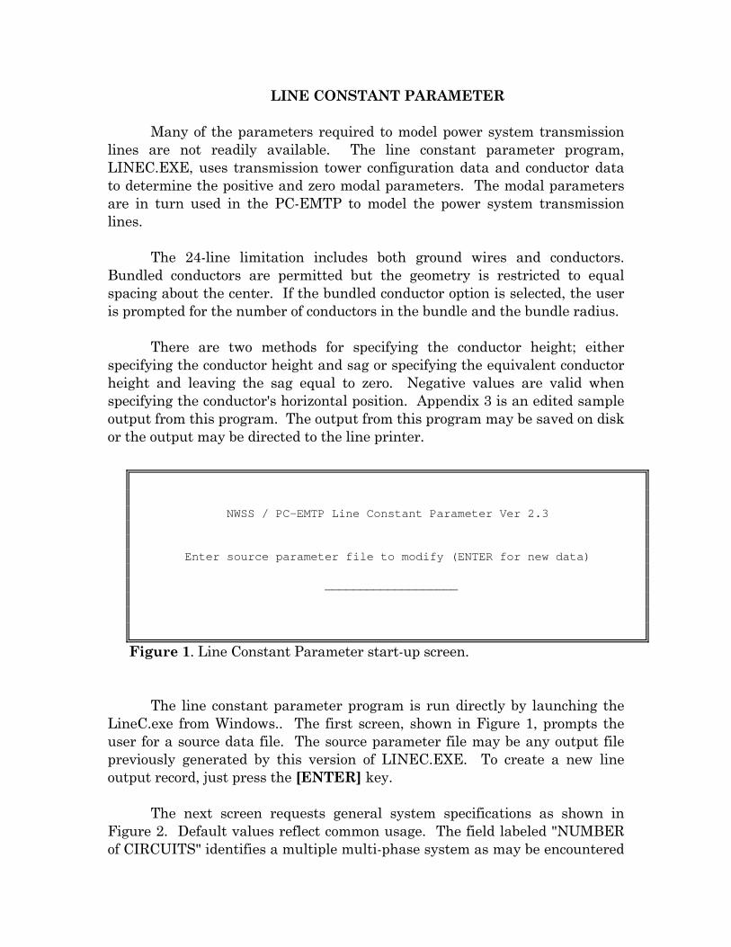
LINE CONSTANT PARAMETER Many of the parameters required to model power system transmission lines are not readily available. The line constant parameter program, LINEC.EXE, uses transmission tower configuration data and conductor data to determine the positive and zero modal parameters. The modal parameters are in turn used in the PC-EMTP to model the power system transmission lines. The 24-line limitation includes both ground wires and conductors. Bundled conductors are permitted but the geometry is restricted to equal spacing about the center. If the bundled conductor option is selected, the user is prompted for the number of conductors in the bundle and the bundle radius. There are two methods for specifying the conductor height; either specifying the conductor height and sag or specifying the equivalent conductor height and leaving the sag equal to zero. Negative values are valid when specifying the conductor's horizontal position. Appendix 3 is an edited sample output from this program. The output from this program may be saved on disk or the output may be directed to the line printer.
The line constant parameter program is run directly by launching the LineC.exe from Windows.. The first screen, shown in Figure 1, prompts the user for a source data file. The source parameter file may be any output file previously generated by this version of LINEC.EXE. To create a new line output record, just press the [ENTER] key. The next screen requests general system specifications as shown in Figure 2. Default values reflect common usage. The field labeled "NUMBER of CIRCUITS" identifies a multiple multi-phase system as may be encountered
NWSS / PC-EMTP Line Constant Parameter Ver 2.3 Enter source parameter file to modify (ENTER for new data) ___________________
Figure 1. Line Constant Parameter start-up screen.
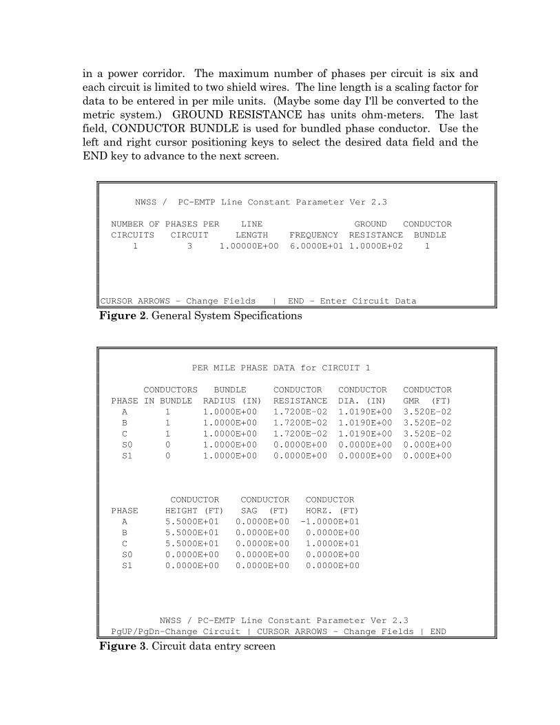
in a power corridor. The maximum number of phases per circuit is six and each circuit is limited to two shield wires. The line length is a scaling factor for data to be entered in per mile units. (Maybe some day I'll be converted to the metric system.) GROUND RESISTANCE has units ohm-meters. The last field, CONDUCTOR BUNDLE is used for bundled phase conductor. Use the left and right cursor positioning keys to select the desired data field and the END key to advance to the next screen.
NWSS / PC-EMTP Line Constant Parameter Ver 2.3 NUMBER OF PHASES PER LINE GROUND CONDUCTOR CIRCUITS CIRCUIT LENGTH FREQUENCY RESISTANCE BUNDLE 1 3 1.00000E+00 6.0000E+01 1.0000E+02 1 CURSOR ARROWS - Change Fields | END - Enter Circuit Data
Figure 2. General System Specifications
PER MILE PHASE DATA for CIRCUIT 1 CONDUCTORS BUNDLE CONDUCTOR CONDUCTOR CONDUCTOR PHASE IN BUNDLE RADIUS (IN) RESISTANCE DIA. (IN) GMR (FT) A 1 1.0000E+00 1.7200E-02 1.0190E+00 3.520E-02 B 1 1.0000E+00 1.7200E-02 1.0190E+00 3.520E-02 C 1 1.0000E+00 1.7200E-02 1.0190E+00 3.520E-02 S0 0 1.0000E+00 0.0000E+00 0.0000E+00 0.000E+00 S1 0 1.0000E+00 0.0000E+00 0.0000E+00 0.000E+00 CONDUCTOR CONDUCTOR CONDUCTOR PHASE HEIGHT (FT) SAG (FT) HORZ. (FT) A 5.5000E+01 0.0000E+00 -1.0000E+01 B 5.5000E+01 0.0000E+00 0.0000E+00 C 5.5000E+01 0.0000E+00 1.0000E+01 S0 0.0000E+00 0.0000E+00 0.0000E+00 S1 0.0000E+00 0.0000E+00 0.0000E+00 NWSS / PC-EMTP Line Constant Parameter Ver 2.3 PgUP/PgDn-Change Circuit | CURSOR ARROWS - Change Fields | END
Figure 3. Circuit data entry screen
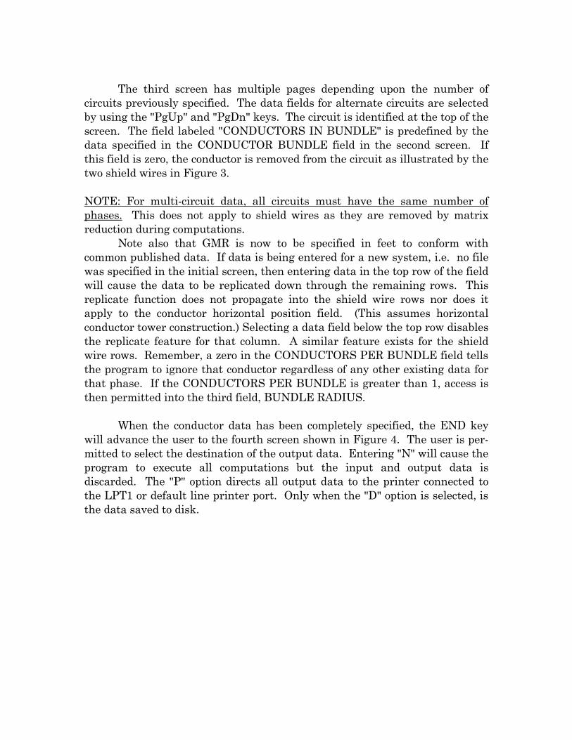
The third screen has multiple pages depending upon the number of circuits previously specified. The data fields for alternate circuits are selected by using the "PgUp" and "PgDn" keys. The circuit is identified at the top of the screen. The field labeled "CONDUCTORS IN BUNDLE" is predefined by the data specified in the CONDUCTOR BUNDLE field in the second screen. If this field is zero, the conductor is removed from the circuit as illustrated by the two shield wires in Figure 3. NOTE: For multi-circuit data, all circuits must have the same number of phases. This does not apply to shield wires as they are removed by matrix reduction during computations. Note also that GMR is now to be specified in feet to conform with common published data. If data is being entered for a new system, i.e. no file was specified in the initial screen, then entering data in the top row of the field will cause the data to be replicated down through the remaining rows. This replicate function does not propagate into the shield wire rows nor does it apply to the conductor horizontal position field. (This assumes horizontal conductor tower construction.) Selecting a data field below the top row disables the replicate feature for that column. A similar feature exists for the shield wire rows. Remember, a zero in the CONDUCTORS PER BUNDLE field tells the program to ignore that conductor regardless of any other existing data for that phase. If the CONDUCTORS PER BUNDLE is greater than 1, access is then permitted into the third field, BUNDLE RADIUS. When the conductor data has been completely specified, the END key will advance the user to the fourth screen shown in Figure 4. The user is per-mitted to select the destination of the output data. Entering "N" will cause the program to execute all computations but the input and output data is discarded. The "P" option directs all output data to the printer connected to the LPT1 or default line printer port. Only when the "D" option is selected, is the data saved to disk.
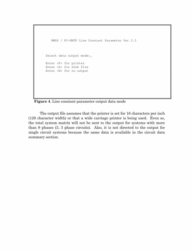
The output file assumes that the printer is set for 16 characters per inch (128 character width) or that a wide carriage printer is being used. Even so, the total system matrix will not be sent to the output for systems with more than 9 phases (3, 3 phase circuits). Also, it is not directed to the output for single circuit systems because the same data is available in the circuit data summary section.
NWSS / PC-EMTP Line Constant Parameter Ver 2.3 Select data output mode:_ Enter <P> for printer Enter <D> for disk file Enter <N> for no output
Figure 4. Line constant parameter output data mode

1
DSP and Power System Protection Richard W. Wall
University of Idaho Department of Electrical Engineering
Moscow, ID 83844-1023 January 30, 2000
(208) 882-8334 [email protected]
Why talk about Power Systems? This article is intended to demonstrate how DSP is used in a particular industry for real-time instrumentation. It is my hope that those in other areas who have similar instrumentation needs can leverage from the digital filtering experience and successes in the power system protection area.
What is power system protection?
The good news is that the electrical power grid did not fail because of any Y2K glitches. This we all know, but do you know why? It was because our power systems have protection. This year I am on sabbatical with a company that makes power system protective relays. For those outside the power industry, power system protection is not money you pay to the godfather to keep your lights on. It is the art and science of the application of devices that monitor the power line currents and voltages and generate signals to deenergize faulted sections of the power grid. The goal is to minimize damage to equipment and property and maintain the delivery of electrical energy to the consumer.
Fifty years ago, electromechanical protective relays were used almost exclusively. In general, these devices use torque generated by AC currents to magnetically close a set of mechanical contacts. The contacts are held open or “restrained” by a mechanical spring much like the common circuit breaker we use in our homes. In reality, these devices were vastly more complicated. Frequently the phase relationships of currents and voltages allowed the relay to determine the direction of the fault relative to the relay. This makes the relays selective resulting in deenergizing only the parts of the power grid that are absolutely necessary to isolate the faulted section. Computer entry into the power protection
Computer based relaying was experimented with in the 50’s and 60’s but were not commercially viable because of the size, expense, and reliability of early computers. Along came the 70’s and the microcontroller revolution, which of course, changed all of that. Believe it or not, the microprocessor-based relays used those same torque relationships that their predecessor electromechanical relays used. Instead of using magnetic flux to generate the torque, the microprocessor relay computed the torque. Modern microprocessor-based relays still use the magnitude and phase of the 60 Hz (50 Hz in Europe) fundamental
2
power voltage and currents to compute torque like quantities that determine the existence of faults.
One of the challenges then (and continues to be today) is how to reliably and efficiently convert sampled analog signals to magnitude and phase needed for the torque equations. Since the fundamental component is the only signal of interest, all other signals, whether they be harmonics, arcing noise or transients generated by exciting the natural modes of the electrical network, are considered noise that corrupts the signal of interest. Schweitzer and Houi reviewed seven of the more common algorithms used to convert a time sequence to a time varying complex vector. Only two of these algorithms are based on orthogonal basis set decomposition similar to the Fourier transform. Discussion in the article will be limited to only one of these algorithms because of its simplicity, efficiency, and performance, the DFT.
Switching domains
The discrete Fourier transform (DFT) is a digital filtering algorithm that computes the magnitude and phase at discrete frequencies of a discrete time sequence. Fast Fourier transforms are computationally efficient algorithms for computing DFTs. FFTs are useful if we need to know the magnitude and/or phase of a number individual or band of frequencies. Jack Crenshaw told us all about Fourier transforms, DFTs and FFT in previous ESP in a series of articles spanning Oct. ’94, through Mar. ’95. But DFTs are simply FIR digital filters and Crenshaw told us “more about filters” (June ‘96), “filters, the very last word” (Sept. ’96) and “filters – a few more words” (Nov. ’96). After Jack said all there was to say, Don Morgan told us about the “fundamentals of FIR design” in a sequence of four ESP articles starting in June ’97. With that plethora of background information, we can jump right into the application.
For protective relaying, we don’t really need to extract the magnitude and phase of every signal contained in the sampled data stream, as is the case of an FFT. This is especially true if there is only one signal present to begin with. If we use a DFT for the only signal we’re interested in, we have both a conversion algorithm and a band bass filter. Theory to application
So let’s try out the theory and see how it works. Lets assume that we are dealing with a 60 Hz signal that is sampled synchronously. This means that the sample interval is the inverse of an integer multiple of 60. We need to compute the DFT for the fundamental using equation (1) where N equals to the number of samples per fundamental cycle, k equal to one for the fundamental, and n is the coefficient subscript. Because digital computers (like most of the world) don’t really understand the concept of imaginary numbers, two digital filters are required, one to get the real part and one for the imaginary part. Mathematically, the coefficients of these filters are by determined using (2).
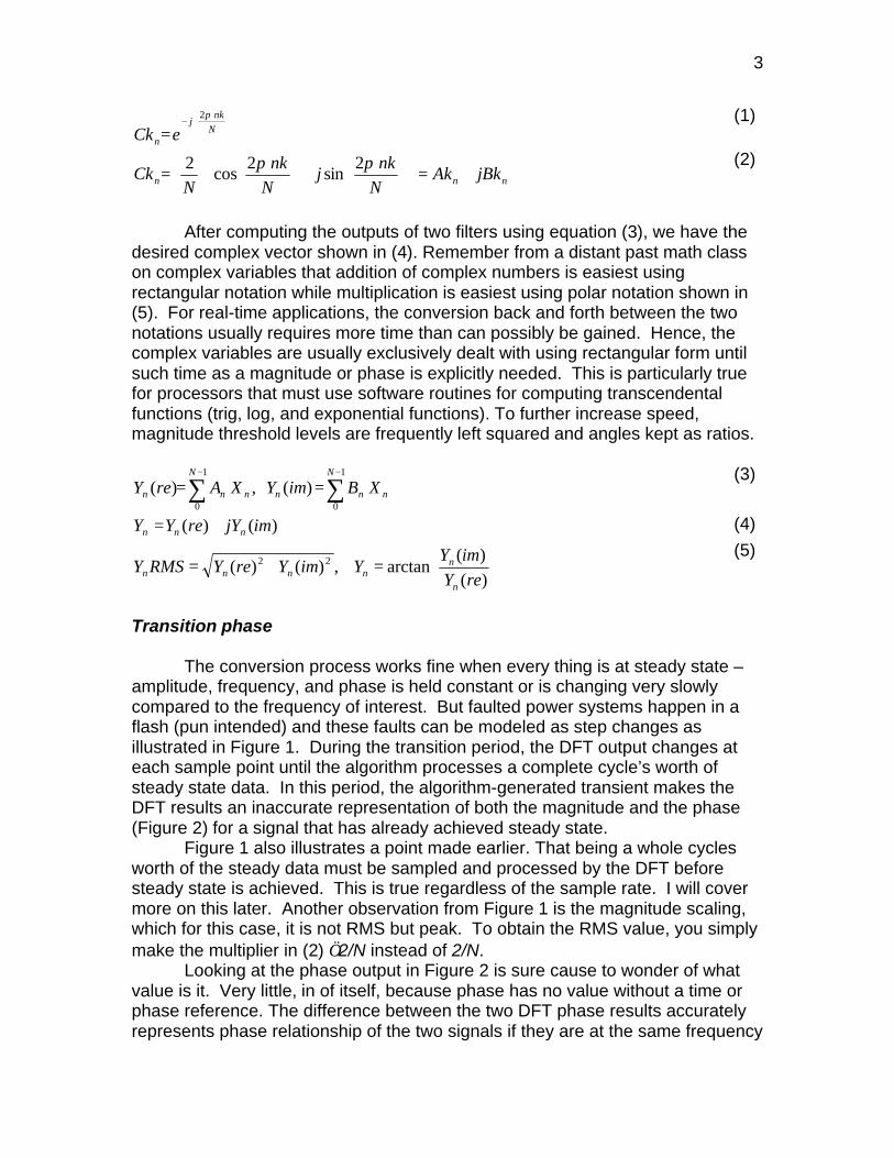
3
−
= N
nkj
n eCkπ2
(1)
nnn jBkAkN
nkj
N
nk
NCk +=
+
=
ππ 2sin
2cos
2
(2)
After computing the outputs of two filters using equation (3), we have the
desired complex vector shown in (4). Remember from a distant past math class on complex variables that addition of complex numbers is easiest using rectangular notation while multiplication is easiest using polar notation shown in (5). For real-time applications, the conversion back and forth between the two notations usually requires more time than can possibly be gained. Hence, the complex variables are usually exclusively dealt with using rectangular form until such time as a magnitude or phase is explicitly needed. This is particularly true for processors that must use software routines for computing transcendental functions (trig, log, and exponential functions). To further increase speed, magnitude threshold levels are frequently left squared and angles kept as ratios.
∑∑−−
==1
0
1
0
)(,)(N
nnn
N
nnn XBimYXAreY (3)
)()( imjYreYY nnn += (4)
=∠+=
)(
)(arctan,)()( 22
reY
imYYimYreYRMSY
n
nnnnn
(5)
Transition phase The conversion process works fine when every thing is at steady state – amplitude, frequency, and phase is held constant or is changing very slowly compared to the frequency of interest. But faulted power systems happen in a flash (pun intended) and these faults can be modeled as step changes as illustrated in Figure 1. During the transition period, the DFT output changes at each sample point until the algorithm processes a complete cycle’s worth of steady state data. In this period, the algorithm-generated transient makes the DFT results an inaccurate representation of both the magnitude and the phase (Figure 2) for a signal that has already achieved steady state.
Figure 1 also illustrates a point made earlier. That being a whole cycles worth of the steady data must be sampled and processed by the DFT before steady state is achieved. This is true regardless of the sample rate. I will cover more on this later. Another observation from Figure 1 is the magnitude scaling, which for this case, it is not RMS but peak. To obtain the RMS value, you simply make the multiplier in (2) √2/N instead of 2/N.
Looking at the phase output in Figure 2 is sure cause to wonder of what value is it. Very little, in of itself, because phase has no value without a time or phase reference. The difference between the two DFT phase results accurately represents phase relationship of the two signals if they are at the same frequency
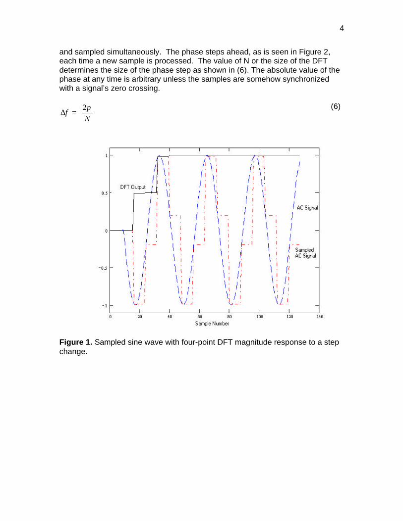
4
and sampled simultaneously. The phase steps ahead, as is seen in Figure 2, each time a new sample is processed. The value of N or the size of the DFT determines the size of the phase step as shown in (6). The absolute value of the phase at any time is arbitrary unless the samples are somehow synchronized with a signal’s zero crossing.
=∆
N
πφ
2
(6)
Figure 1. Sampled sine wave with four-point DFT magnitude response to a step change.
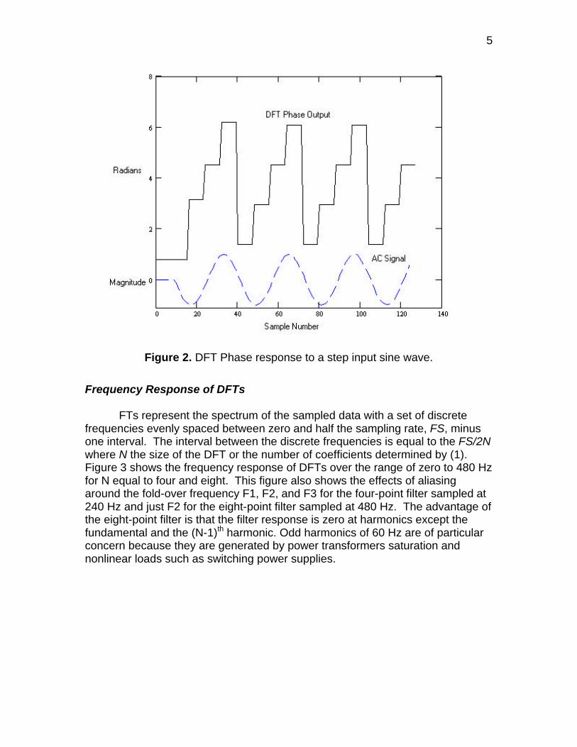
5
Figure 2. DFT Phase response to a step input sine wave.
Frequency Response of DFTs
FTs represent the spectrum of the sampled data with a set of discrete frequencies evenly spaced between zero and half the sampling rate, FS, minus one interval. The interval between the discrete frequencies is equal to the FS/2N where N the size of the DFT or the number of coefficients determined by (1). Figure 3 shows the frequency response of DFTs over the range of zero to 480 Hz for N equal to four and eight. This figure also shows the effects of aliasing around the fold-over frequency F1, F2, and F3 for the four-point filter sampled at 240 Hz and just F2 for the eight-point filter sampled at 480 Hz. The advantage of the eight-point filter is that the filter response is zero at harmonics except the fundamental and the (N-1)th harmonic. Odd harmonics of 60 Hz are of particular concern because they are generated by power transformers saturation and nonlinear loads such as switching power supplies.
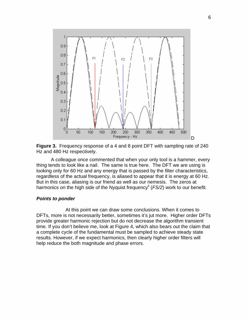
6
D
Figure 3. Frequency response of a 4 and 8 point DFT with sampling rate of 240 Hz and 480 Hz respectively.
A colleague once commented that when your only tool is a hammer, every thing tends to look like a nail. The same is true here. The DFT we are using is looking only for 60 Hz and any energy that is passed by the filter characteristics, regardless of the actual frequency, is aliased to appear that it is energy at 60 Hz. But in this case, aliasing is our friend as well as our nemesis. The zeros at harmonics on the high side of the Nyquist frequencyii (FS/2) work to our benefit. Points to ponder
At this point we can draw some conclusions. When it comes to DFTs, more is not necessarily better, sometimes it’s jut more. Higher order DFTs provide greater harmonic rejection but do not decrease the algorithm transient time. If you don’t believe me, look at Figure 4, which also bears out the claim that a complete cycle of the fundamental must be sampled to achieve steady state results. However, if we expect harmonics, then clearly higher order filters will help reduce the both magnitude and phase errors.
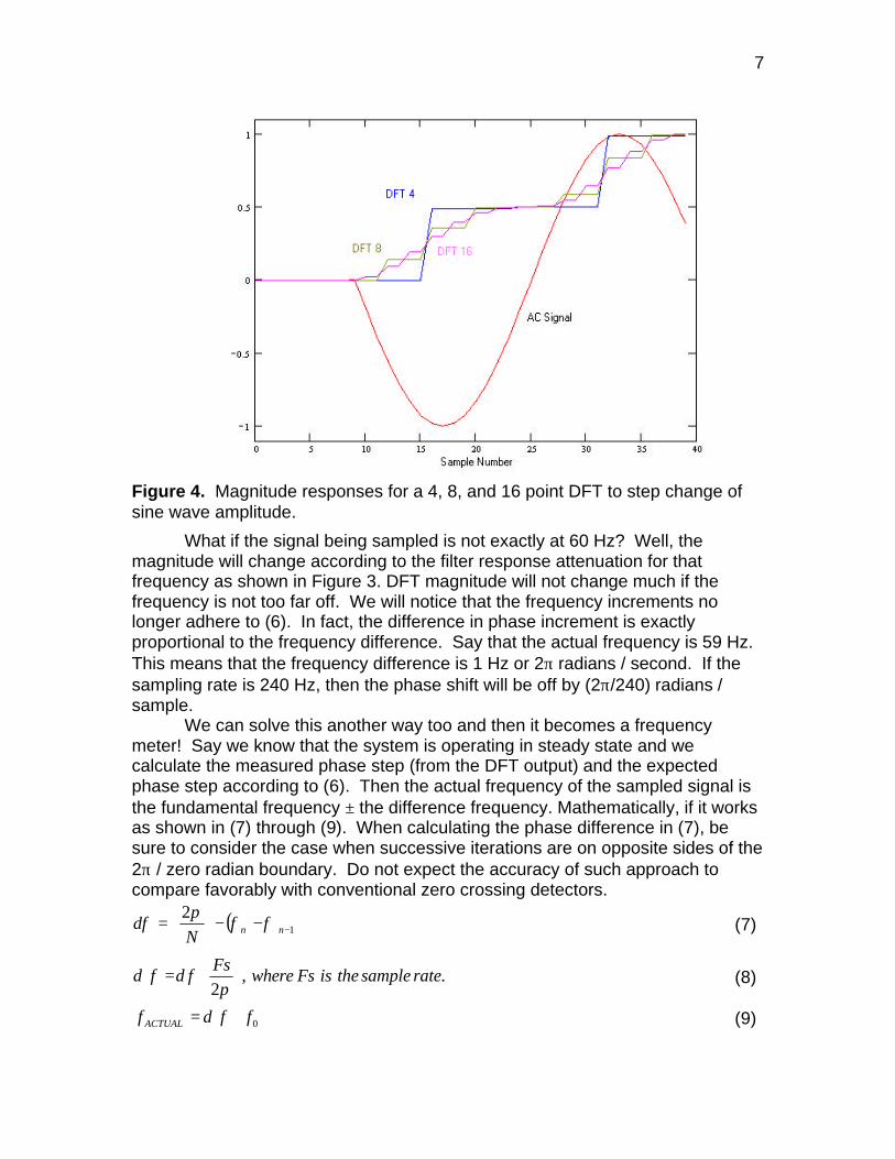
7
Figure 4. Magnitude responses for a 4, 8, and 16 point DFT to step change of sine wave amplitude.
What if the signal being sampled is not exactly at 60 Hz? Well, the magnitude will change according to the filter response attenuation for that frequency as shown in Figure 3. DFT magnitude will not change much if the frequency is not too far off. We will notice that the frequency increments no longer adhere to (6). In fact, the difference in phase increment is exactly proportional to the frequency difference. Say that the actual frequency is 59 Hz. This means that the frequency difference is 1 Hz or 2π radians / second. If the sampling rate is 240 Hz, then the phase shift will be off by (2π/240) radians / sample.
We can solve this another way too and then it becomes a frequency meter! Say we know that the system is operating in steady state and we calculate the measured phase step (from the DFT output) and the expected phase step according to (6). Then the actual frequency of the sampled signal is the fundamental frequency ± the difference frequency. Mathematically, if it works as shown in (7) through (9). When calculating the phase difference in (7), be sure to consider the case when successive iterations are on opposite sides of the 2π / zero radian boundary. Do not expect the accuracy of such approach to compare favorably with conventional zero crossing detectors.
( )1
2−−−
= nnN
φφπ
δφ (7)
.,2
ratesampletheisFswhereFs
f
=
πφδδ (8)
0fff ACTUAL += δ (9)
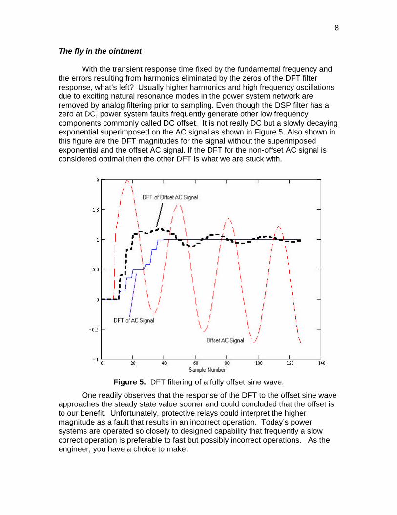
8
The fly in the ointment With the transient response time fixed by the fundamental frequency and the errors resulting from harmonics eliminated by the zeros of the DFT filter response, what’s left? Usually higher harmonics and high frequency oscillations due to exciting natural resonance modes in the power system network are removed by analog filtering prior to sampling. Even though the DSP filter has a zero at DC, power system faults frequently generate other low frequency components commonly called DC offset. It is not really DC but a slowly decaying exponential superimposed on the AC signal as shown in Figure 5. Also shown in this figure are the DFT magnitudes for the signal without the superimposed exponential and the offset AC signal. If the DFT for the non-offset AC signal is considered optimal then the other DFT is what we are stuck with.
Figure 5. DFT filtering of a fully offset sine wave.
One readily observes that the response of the DFT to the offset sine wave approaches the steady state value sooner and could concluded that the offset is to our benefit. Unfortunately, protective relays could interpret the higher magnitude as a fault that results in an incorrect operation. Today’s power systems are operated so closely to designed capability that frequently a slow correct operation is preferable to fast but possibly incorrect operations. As the engineer, you have a choice to make.
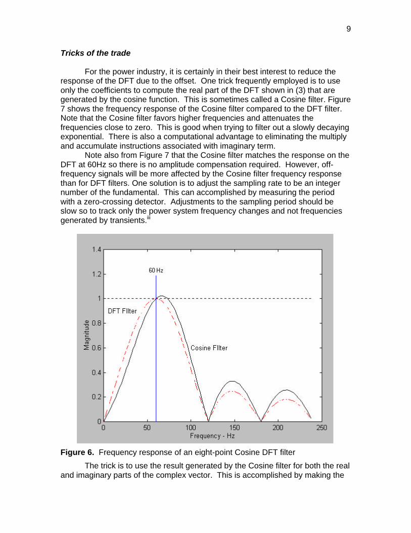
9
Tricks of the trade For the power industry, it is certainly in their best interest to reduce the response of the DFT due to the offset. One trick frequently employed is to use only the coefficients to compute the real part of the DFT shown in (3) that are generated by the cosine function. This is sometimes called a Cosine filter. Figure 7 shows the frequency response of the Cosine filter compared to the DFT filter. Note that the Cosine filter favors higher frequencies and attenuates the frequencies close to zero. This is good when trying to filter out a slowly decaying exponential. There is also a computational advantage to eliminating the multiply and accumulate instructions associated with imaginary term.
Note also from Figure 7 that the Cosine filter matches the response on the DFT at 60Hz so there is no amplitude compensation required. However, off-frequency signals will be more affected by the Cosine filter frequency response than for DFT filters. One solution is to adjust the sampling rate to be an integer number of the fundamental. This can accomplished by measuring the period with a zero-crossing detector. Adjustments to the sampling period should be slow so to track only the power system frequency changes and not frequencies generated by transients.iii
Figure 6. Frequency response of an eight-point Cosine DFT filter
The trick is to use the result generated by the Cosine filter for both the real and imaginary parts of the complex vector. This is accomplished by making the
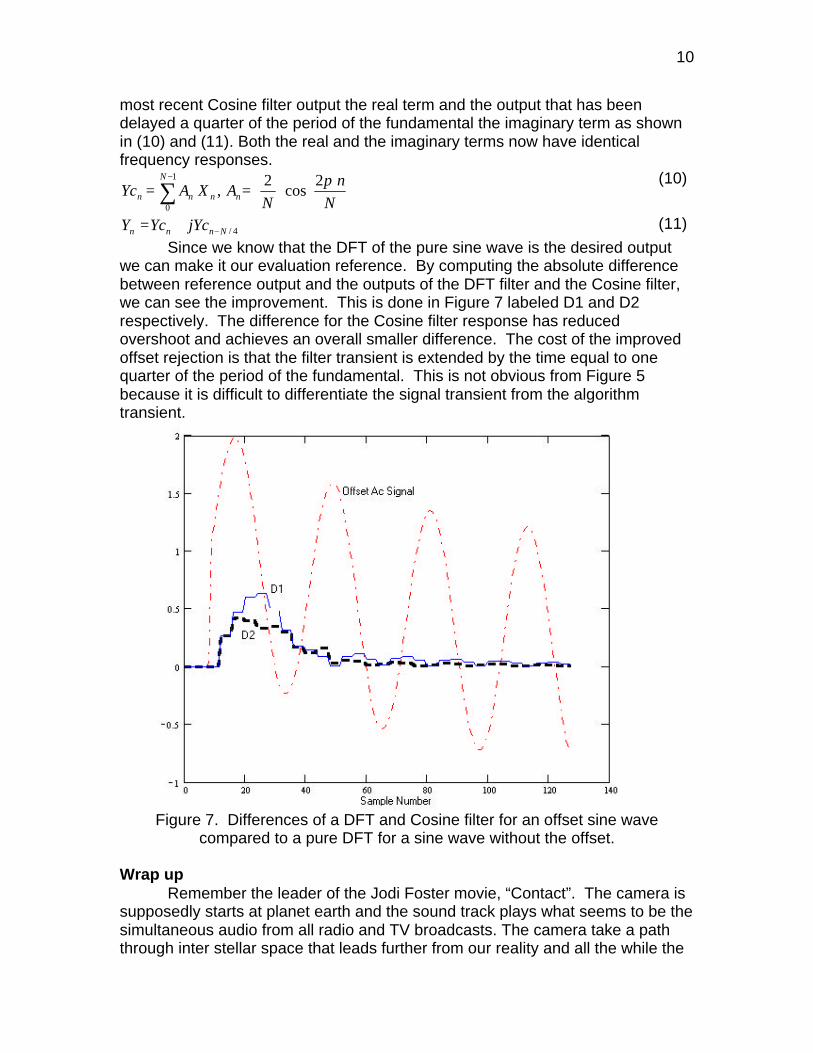
10
most recent Cosine filter output the real term and the output that has been delayed a quarter of the period of the fundamental the imaginary term as shown in (10) and (11). Both the real and the imaginary terms now have identical frequency responses.
== ∑
−
N
n
NAXAYc n
N
nnn
π2cos
2,
1
0
(10)
4/Nnnn jYcYcY −+= (11)
Since we know that the DFT of the pure sine wave is the desired output we can make it our evaluation reference. By computing the absolute difference between reference output and the outputs of the DFT filter and the Cosine filter, we can see the improvement. This is done in Figure 7 labeled D1 and D2 respectively. The difference for the Cosine filter response has reduced overshoot and achieves an overall smaller difference. The cost of the improved offset rejection is that the filter transient is extended by the time equal to one quarter of the period of the fundamental. This is not obvious from Figure 5 because it is difficult to differentiate the signal transient from the algorithm transient.
Figure 7. Differences of a DFT and Cosine filter for an offset sine wave
compared to a pure DFT for a sine wave without the offset. Wrap up Remember the leader of the Jodi Foster movie, “Contact”. The camera is supposedly starts at planet earth and the sound track plays what seems to be the simultaneous audio from all radio and TV broadcasts. The camera take a path through inter stellar space that leads further from our reality and all the while the
11
audio becomes more focused on fewer and fewer broadcasts. Finally, we’re left with a single radio transmission of a young girl on a ham radio. I feel that this article has taken a similar path.
The idea here is that we’re interested signals at one frequency only and we needed an algorithm that quickly and accurately computes the magnitude and phase of that signal. We can take advantage of aliasing to cancel harmonics if we don’t expect that the signal will contain energy that is also passed by the aliasing. DSP tricks can improve performance but always come at a price. It is the responsibility of the designer to understand the application sufficiently to know where compromises are tolerable to achieve the desired performance.
Final words of caution The voltages on lines that deliver power make them lethal. Relays cannot operate fast enough to prevent serious injury or death to someone coming in contact with an energized power line. In an emergency situation, never assume that relays have operated and the lines are deenergized. One of the most difficult conditions to detect is a distribution line that broken and fallen to the ground. The fault current is so small that most relays cannot sense the fault. Always assume power lines are energized and treat them accordingly. i E.O. Schweitzer and D. Hou, “Filtering for Protective Relays”, 47th Annual Georgia Tech Protective Relay Conference, Atlanta GA. April 28-30, 1993. This article is available for download in PDF format at http://www.selinc.com/techpprs.htm. ii Digital Filtering: an Introduction, Edward P. Cunningham, Houghton Mifflin Co., 1992, ISBN 0-395-53989-7 iii R.W. Wall and H.L. Hess, “Design of Microcontroller Implementation of a Three Phase SCR Power Converter”, Journal of Circuits, Systems, and Computers, Vol. 6. No. 6. Mar. 1997, pp. 619-633.