Power System State Estimation and Optimal Measurement

Power System State Estimationand Optimal Measurement Placementfor Distributed Multi-Utility Operation

Final Project Report

Power Systems Engineering Research Center

A National Science FoundationIndustry/University Cooperative Research Center

since 1996

PSERC

Power Systems Engineering Research Center

Power System State Estimation and Optimal Measurement Placement for Distributed Multi-Utility Operation

Final Project Report

Project Team

Ali Abur, Garng M. Huang Texas A&M University

PSERC Publication 02-45

November 2002

Information about this Project For information about this project contact: A. Abur Professor Texas A&M University Department of Electrical Engineering College Station, TX 77843-3128 Phone: 979 845 1493 Fax: 979 845 9887 Email: [email protected] Power Systems Engineering Research Center This is a project report from the Power Systems Engineering Research Center (PSERC). PSERC is a multi-university Center conducting research on challenges facing a restructuring electric power industry and educating the next generation of power engineers. More information about PSERC can be found at the Center’s website: http://www.pserc.wisc.edu. For additional information, contact: Power Systems Engineering Research Center Cornell University 428 Phillips Hall Ithaca, New York 14853 Phone: 607-255-5601 Fax: 607-255-8871 Notice Concerning Copyright Material PSERC members are given permission to copy without fee all or part of this publication if appropriate attribution is given to this document as the source material. This report is available for downloading from the PSERC website.

2002 Texas A&M University. All rights reserved.

http://www.pserc.wisc.edu/../../../../../../WINDOWS/TEMP/Documents and Settings/b0x7826/Local Settings/Temp/[email protected]

http://www.pserc.wisc.edu/

ACKNOWLEDGEMENTS

The work described in this report was sponsored by the Power Systems Engineering Research

Center (PSERC). We express our appreciation for the support provided by PSERC’s industrial

members and by the National Science Foundation under grant NSF EEC 0002917 received

under the Industry / University Cooperative Research Center program.

The industry advisors for the project were Mani Subramanian, ABB Network Management;

Don Sevcik, CenterPoint Energy; and Bruce Dietzman, Oncor. Their suggestions and

contributions to the work are appreciated.

ii

EXECUTIVE SUMMARY

The new power markets induce changes in the way the transmission grid is operated and, as a

result, an increased number of power transactions take place creating unanticipated power

flows through the system. Monitoring these flows reliably and accurately requires a robust

measurement system. Furthermore, unlike conventional systems, modern power systems are

equipped with advanced power flow controllers or flexible A.C. transmission system (FACTS)

devices for redirecting power flows to handle congestion. Monitoring these devices and their

parameters is also becoming important. Finally, existence of multiple ISOs/RTOs, and

associated inter-utility power exchanges, presents a need for addressing the multi-utility data

exchange issues in the new power market environment. Accordingly, the project is divided into

two parts. The first part is on the meter placement while the second part focuses on the

distributed state estimator for multi-utility data exchanges.

For the first part, a systematic method is developed for placing meters either to upgrade an

existing measurement system or to build one from scratch. This method not only ensures

observability of the system for a base case operating topology, but also accounts for expected

contingencies and measurement losses. In order to address the issue of FACTS devices, a new

estimator is developed. This estimator is capable of incorporating the power flow controllers,

along with their operating and parameter limits, into the state estimation formulation.

For the second part, we are focusing on the following scenario.

With power market deregulation, member companies cooperate to share one whole grid

system and try to achieve their own economic goals. The companies release operational

control of their transmission grids to form ISOs/RTOs while maintaining their own state

estimators over their own areas.

This project also focuses on how to improve the state estimation result of member companies

or the ISO by exchanging raw or estimated data with neighboring member companies (or

ISOs). Numerical tests verify that selected data exchange improves the estimator quality of

individual entities for both estimation reliability and estimation accuracy. It is also shown that

iii

the benefit of alternative data exchange schemes can be quite different; some data exchanges

are even harmful if our principles are not carefully followed.

Another recent trend for these ISOs/RTOs is to combine and grow to form a Mega-RTO grid

for a better market efficiency. The determination of state over the whole system becomes

challenging due to its large size. Instead of a totally new estimator over the whole grid, we

propose a distributed textured algorithm to determine the whole state; in our algorithm, the

existing state estimators in local companies/ISOs/RTOs are fully utilized and the new

estimator is no longer required. We need only some extra communication for some

instrumentation or estimated data exchange. Detailed numerical tests are given to verify the

efficiency and validity of the new approach.

The developed methods of this project are implemented in the form of prototype software.

Simulations were carried out on test systems and the results are provided in this report.

iv

TABLE OF CONTENTS

Part I: State Estimation of Power Systems Embedded with FACTS Devices....................1

I. INTRODUCTION......................................................................................................1 1.1 Introduction ..............................................................................................................1 1.2 Problem Statement ...................................................................................................1

II. PROPOSED ALGORITHM .....................................................................................2 2.1 Steady state model of UPFC ....................................................................................2 2.2 HACHTEL’s augmented matrix method [3,4].........................................................4 2.3 Observability Analysis .............................................................................................6 2.4 Equations ..................................................................................................................6 2.4.1 Lines without an installed UPFC ..........................................................................6 2.4.2 Lines controlled by a UPFC..................................................................................7 2.5 Algorithm .................................................................................................................8

III. NUMERICAL EXAMPLES .....................................................................................9 3.1 14-bus system ...........................................................................................................9 3.2 30-bus system .........................................................................................................15 3.3 Conclusion..............................................................................................................22

REFERENCES ...................................................................................................................22

Part II: Optimal Meter Placement for Maintaining Network Observability Under

Contingencies..........................................................................................................................23

I. INTRODUCTION....................................................................................................23 1.1 Introduction ............................................................................................................23 1.2 Problem Statement .................................................................................................24

II. PROPOSED ALGORITHM ...................................................................................25 2.1 H matrix..................................................................................................................25 2.2 Candidate measurements identification..................................................................26 2.3 Optimal Meter Placement.......................................................................................29 2.4 Algorithm ...............................................................................................................30

III. NUMERICAL EXAMPLES ...................................................................................31 3.1 6-bus system ...........................................................................................................31 3.2 14-bus system .........................................................................................................34 3.3 30-bus system .........................................................................................................37 3.4 57-bus system .........................................................................................................41 3.5 Conclusions ............................................................................................................45

REFERENCES ...................................................................................................................45

v

Part III: Design of Data Exchange on Distributed Multi-Utility Operations...................46

I. INTRODUCTION....................................................................................................46

II. BUS CREDIBILITY INDEX (BCI) .......................................................................48 2.1 Basic analysis of state estimation...........................................................................48 2.2 Critical p-tuples ......................................................................................................49 2.3 Weak Bus Sets of Critical p-tuples.........................................................................50 2.4 Bus Redundancy Descriptor (BRD) .......................................................................50 2.5 A new concept of Bus Credibility Index (BCI)......................................................51 2.6 Remarks..................................................................................................................52

III. KNOWLEDGE BASE .............................................................................................53 1. Raw Facts ...............................................................................................................53 2. BCI Information .....................................................................................................53 3. Variance of SE errors .............................................................................................54

IV. REASONING MACHINE.......................................................................................54

V. NUMERICAL TESTS ...................................................................................................59 5.1 Case 1: Harmful Data Exchange Scheme...............................................................59 5.2 Case 2: Efficiency of Beneficial Data Exchange ...................................................60 5.3 Case 3: Impact on New Measurement Placement (1) ............................................61 5.4 Case 4: Impact on New Measurement Placement (2) ............................................61

VI. CONCLUSION ........................................................................................................62

REFERENCES ...................................................................................................................62

Part IV: A Concurrent Textured Distributed State Estimation Algorithm.....................64

I. INTRODUCTION....................................................................................................64

II. CONCURRENT TEXTURED DSE ALGORITHM ............................................66 2.1 Existing DSE Algorithms and their Drawbacks.....................................................66 2.2 Introduction of a New Algorithm...........................................................................67 2.3 Main Algorithm......................................................................................................67 2.4 Advantages of the New Algorithm.........................................................................68

III. DSE TEXTURED DECOMPOSITION METHOD .............................................69 3.1 Introduction ............................................................................................................69 3.2 A Systematic Textured Decomposition Method ....................................................70 3.3 Numerical Examples ..............................................................................................70

IV. ESTIMATED DATE EXCHANGE ........................................................................72 4.1 Sparse Technique for Matrix Modification ............................................................72 4.2 Application of the Sparse Technique .....................................................................73

V. DETERMINATION OF STATE OVER WHOLE GRID ....................................75

vi

VI. NUMERICAL RESULTS........................................................................................76 6.1 Case 1: Accuracy and Discrepancy ........................................................................76 6.2 Case 2: Effect of textured instrumentation data exchange (1) ...............................77 6.3 Case 3: Effect of textured instrumentation data exchange (2) ...............................77 6.4 Case 4: Effect of estimated data exchange.............................................................78

VII. CONCLUSIONS ......................................................................................................79

REFERENCES....................................................................................................................79

Project Publications ...............................................................................................................81

Project Conclusions ...............................................................................................................82

1

PART I: STATE ESTIMATION OF POWER SYSTEMS

EMBEDDED WITH FACTS DEVICES

I. INTRODUCTION

1.1 Introduction

After the establishment of power markets with transmission open access, the significance and use

of FACTS devices for manipulating line power flows to relieve congestion and optimize the

overall grid operation have increased. As a result, there is a need to integrate the FACTS device

models into the existing power system applications. This report will present an algorithm for state

estimation of network embedded with FACTS devices. Furthermore, it will be shown via case

studies that the same estimation program can also be used for determining the controller setting

for a desired operating condition.

There are several kinds of FACTS devices. Thyristor-switched series capacitors (TCSC) and

thyristor-switched phase shifting transformer (TCPST) can exert a voltage in series with the line

and, therefore, can control the active power through a transmission line [3]. On the other hand, the

Unified Power Flow Controller (UPFC) has a series voltage source and a shunt voltage source,

allowing independent control of the voltage magnitude, and the real and reactive power flows

along a given transmission line [1,2]. In this report, only one device, namely the UPFC, will be

considered due to its complexity and versatility in controlling power flows.

1.2 Problem Statement

Flexible A.C. transmission systems [FACTS] are being used more in large power systems for

their significance in manipulating line power flows. Traditional state estimation methods without

integrating FACTS devices will not be suitable for power systems embedded with FACTS.

State estimation in power system can be formulated as a nonlinear weighted least squares (WLS)

problem. It has a set of measurement equations: ε+= )(xhz ; a set of equality constraints

0)( =xc , representing the zero injections of buses and the zero active power exchange between

2

the power system and FACTS devices; a set of inequality constraints sxf ≤)( , representing the

Var limits on generators, transformer tap ratio limits, and the power and voltage limit of FACTS

devices.

This report will present an algorithm to solve this nonlinear weighted least squares problem. By

solving the problem we can not only estimate the state variables (bus voltages and phase angles)

of power system, but can also determine the controller settings of FACTS devices for a desired

operating condition.

In this report, an approach that incorporates FACTS devices into the state estimation will be

presented. First, a steady-state model of the UPFC [1,2] with operating and parameters limits will

be introduced. Then, the commonly used Hatchtel’s augmented matrix method [3,4] will be used

to implement a numerically robust and computationally efficient state estimator, which is also

flexible enough to account for various device constraints. To treat the inequality constraints, we

will introduce the Logarithmic barrier function method [5] and integrate it into Hatchtel’s matrix.

Simulation results for typical systems are shown at the end of part one. It will be shown via case

studies that this program can also be used for determining the controller settings of a UPFC for a

desired operating condition.

II. PROPOSED ALGORITHM

2.1 Steady state model of UPFC

The Unified Power Flow Controller (UPFC) [1,2] can control the voltage magnitude, real and

reactive power flows simultaneously. The real physical model of UPFC consists of two switching

converters as illustrated in Figure 1.1. These inverters are operated from a common dc link

provided by a dc storage capacitor. This arrangement functions as an ideal ac to ac power

converter in which the real power can freely flow in either direction between the ac terminals of

the two inverters and each inverter can independently generate (or absorb) reactive power at its

own ac output terminal [2].

3

Fig. 1.1 Basic circuit arrangement of the Unified Power Flow Controller

The steady state model of UPFC consists of two ideal voltage sources, one in series and one in

parallel with the associated line, as shown in Figure 1.2. Neglecting UPFC losses, during

steady-state operation it neither absorbs nor injects real power into the system [2].

Fig. 1.2 Steady state model of UPFC

The constraint 0=+ EB PP in Figure 1.2 has two implications.

No real-power is exchanged between the UPFC and the system.

The two sources are mutually dependent.

The real and reactive power going through line k-m can be formulated by equations (1.1) to (1.4).

BkB

BkEk

E

Ekkm

B

mkkm X

VVX

VVX

VVP ,, sinsinsin θθθ −+= (1.1)

BkB

BkEk

E

Ekkm

B

mkk

EB

EEkm X

VVX

VVX

VVV

XXXXQ ,,

2 coscoscos θθθ +−−+= (1.2)

BBV δ∠BZ

BI

EEV δ∠ 0=+ EB PP

EIEZ

4

BmB

Bmmk

B

mkmk X

VVX

VVP ,sinsin θθ += (1.3)

BmB

Bmmk

B

mk

B

mmk X

VVX

VVX

VQ ,

2

coscos θθ −−= (1.4)

Variables BBEE VV θθ ,,, are the control parameters of the UPFC. There are equality and

inequality constraints for the UPFC, which can be formulated by equations (1.5) to (1.9).

Real Power Constraints: 0=+ BE PP (1.5)

Shunt Power Constraints: max,22

EEE TQP ≤+ (1.6)

Series Power Constraints: max,22

BBB TQP ≤+ (1.7)

Shunt Voltage Constraints: max,BB VV ≤ (1.8)

Series Voltage Constraints: max,EE VV ≤ (1.9) 2.2 HACHTEL’s augmented matrix method [3,4]

Power system state estimation problem can be formulated as a nonlinear least squares problem

with a set of equality and inequality constraints [6].

Min rRr T 1

21 −

s.t.

0000

)()(

)(

≥===

+−

+

sxhzr

xcsxf

(1.10)

rxhz += )( represents the equations for measurements, where z is the (mx1) measurement

vector, h(.) is the (mx1) vector of nonlinear functions, “x” is the (nx1) state vector, “r” is the

(mx1) measurement error vector.

0)( =xc represents the equality constraints, where )(⋅c is the ( 1×r ) vector of nonlinear

functions. These equality constraints represent the zero injection buses and the zero active power

exchange between the system and the FACTS devices.

5

0)( ≤xf represents the inequality constraints, which represent the Var limits on generators, ratio

limits of transformer taps, and the power and voltage limits of the UPFC

( max,22

EEE TQP ≤+ , max,22

BBB TQP ≤+ , max,BB VV ≤ , max,EE VV ≤ ).

s is a vector of slack variables used to convert the inequality constraints to equality constraints.

In order to solve the problem of (1.10), we will employ the interior point optimization method. In

this method, the slack variables are treated by appending a logarithmic barrier function to the

objective function,

where p is the number of inequality constraints and ks is the kth element of the slack variable

vector s . The barrier parameter 0>µ is forced to decrease towards zero as the iterations

progress.

The Lagrangian function is given by (1.12).

[ ] [ ])()()(ln21

1

1 xhzrxgsxfsrRrL TTTp

kk

T +−−−+−−= ∑=

− πρλµµ (1.12)

By using the Kuhn-Karroush-Tucker (KKT) optimality conditions and replacing the

nonlinear functions by their first order approximations, the solution to the nonlinear least

squares problem will be obtained by iteratively solving the following linear equations:

−−−

=

∆

⋅

0)(

)()(

000

00000

k

k

k

TTT

xhzxgxf

xHGFHRGFD

πρλ

(1.13)

∑=

− −=p

kk

T srRr1

1 ln21 µφµ (1.11)

6

The matrix on the left side will be referred as the K matrix. Matrices F , G , H are the

gradient matrices of the functions )(xf , )(xg , )(xh respectively. D is built as (1.14),

where S is the diagonal matrix whose kth diagonal element is ks .

2)(1 SDµ

= (1.14)

Solving (1.13) iteratively yields the solution for (1.10).

2.3 Observability Analysis

Observability analysis can be carried out using the numerical method. The Jacobian

matrix

HGF

will be decomposed into its lower and upper rectangular factors using the

Peter-Wilkinson method. In the case of zero pivots, pseudo-measurements will be added to

make the system observable. The pseudo-measurements will indicate deficiencies in the

measurement system, both for the network states as well as for the FACTS device

parameters.

2.4 Equations

This section provides the detailed equations for the measurements incident to a given line, both with and without a UPFC device.

2.4.1 Lines without an installed UPFC

Consider two possible measurements (1 and 2) on line k-m.

Fig. 1.3 Candidate measurements on line k-m without UPFC

Equations for meter 1 are:

7

∑≠=

++=n

kjjkjkjkjkjjkkkkk BGVVGVP

,1

2 )sincos( θθ (1.15)

∑≠=

−+−=n

kjjkjkjkjkjjkkkkk BGVVBVQ

,1

2 )cossin( θθ (1.16)


)sincos(2kmkmkmkmmkkmkk BGVVGVP θθ ++−= (1.17)

)cossin()(2kmkmkmkmmkkmkmkk BGVVCBVQ θθ −+−= (1.18)

2.4.2 Lines controlled by a UPFC

Fig. 1.4 UPFC and candidate measurements on line k-m

Suppose a UPFC is installed on line k-m. Measurements 1, 2, 3, 4 are the measurements that

can be placed on line k-m.


kEEEkkkBkkkBBBk

n

mkjj

kjkjkjkjjkkmkkkk

BVVBVVBVV

BGVVGGVP

θθθ

θθ

sinsinsin

)sincos()(

''

,1

2

−−+

+++= ∑≠= (1.19)

kEEEkkkBkkkBBBk

n

mkjj

kjkjkjkjjkEBkmkkkk

BVVBVVBVV

BGVVBBBBVQ

θθθ

θθ

coscoscos

)cossin()(

''

,1

2

++−

−++++−= ∑≠= (1.20)


BkBBkkkBkkkm BVVBVVP '''' sinsin θθ += (1.21)

BkBBkkkBkkBkkm BVVBVVBVQ ''''2' coscos θθ −−= (1.22)

and

meter 1

m jXR +k’

UPFC k

meter 2 meter 3

meter 4

8

)sincos( '''2' mkkmmkkmmkkmkkm BGVVGVP θθ ++−= (1.23)

)cossin()( '''02' mkkmmkkmmkkmkmkkm BGVVCBVQ θθ −+−= (1.24)


)sincos(

)sincos(''

'2

mBkmmBkmBm

mkkjmkjkjkmkmmmk

BGVV

BGVVGVP

θθ

θθ

++

++−= (1.25)

)cossin(

)cossin()(''

0'2

mBkmmBkmBm

mkkjmkjkjkmmkkmmmk

BGVV

BGVVCBVQ

θθ

θθ

−+

−+−= (1.26)


)sincos()sincos(

)sincos()(

''''

,1

'2

mBkmmBkmBmmkkmmkkmkm

n

mkjj

mjmjmjmjjmkmmkmmmm

BGVVBGVV

BGVVGGGVP

θθθθ

θθ

++++

++−+= ∑≠= (1.27)

)cossin()cossin(

)cossin()(

''''

,1

'2

mBkmmBkmBmmkkmmkkmkm

n

mkjj

mjmjmjmjjmkmmkmmmm

BGVVBGVV

BGVVBBBVQ

θθθθ

θθ

−+−+

−+−+−= ∑≠= (1.28)

2.5 Algorithm

The following algorithm is used in this program of state estimation. It is based upon the

previously presented analysis and the reader is referred to the previous sections for the

notation used in the following description of algorithm steps.

Step 1: Read network data and measurements.

Step 2: Initialize: )(kx , k = 0.

Step 3: Form )(kK matrix.

9

Step 4: Calculate the equality and inequality constraints, measurements mismatch, and form

the right hand side b vector.

−−−

=

0)(

)()(

)(k

k

k

k

xhzxgxf

b .

Step 5: Solve the equation: )()( kk b

x

K =

∆

⋅πρλ

, get )(kx∆ .

Step 6: Update x : )()()1( kkk xxx ∆+=+.

Step 7: Terminate execution if ε≤∆−∆ − )1()( kk xx , and go to step 8, else, k = k+1 and go to

step 3.

Step 8: Stop and print out results.

III. NUMERICAL EXAMPLES

3.1 14-bus system

Fig. 1.5 IEEE-14 system

10

IEEE-14 bus system is shown in Figure 1.5. A FACTS device (UPFC) is installed on line

6-12, near bus 6. The parameters of UPFC are shown below.

Parameters of the installed UPFC device:

From (bus) To (bus) BX EX max,BV max,EV max,BS max,ES

6 12 0.7 0.7 1.0 1.0 1.0 1.0

The developed program can be utilized in two different ways depending upon the purpose of

the study. It can be used as an estimator of the FACTS device parameters for a given set of

measurements. The estimation will yield not only the system states but also the FACTS

device parameters. It can also be utilized as a tool to estimate the required values for the

parameters of the FACTS devices in order to maintain a specific level of flow through a

specified line. The amount of desired power flow through line 6-12, which happens to have a

FACTS device installed on it, can be maintained by the use of this program and estimating

the required settings of the control variables of this FACTS device.

First, the function of the program as an estimator will be illustrated.

Suppose that the system has voltage magnitude, bus injection and line flow measurements.

The measurement values are shown below.

Voltage Measurements:

Bus No. Voltage Bus No. Voltage 4 1.01870 14 1.03700

Bus Injection Measurements:

Bus No. P Q Bus No. P Q 3 -0.94200 0.04393 5 -0.07600 0.01600 6 -0.11200 0.04718 7 0.00000 0.00000 8 0.00000 0.17357 9 -0.29500 -0.16600 10 -0.09000 -0.05800 11 -0.03500 -0.01800 13 -0.13500 -0.05800

11

Line Flow Measurements:

Bus No. (From) Bus No. (To) Active Power P Reactive Power Q 1 2 1.56771 -0.20378 2 3 0.73161 0.03568 4 7 0.27870 -0.09478 9 14 0.08801 0.03591 6 13 0.13670 0.07187 6 12 0.12464 0.02372

The program is executed and all the unknown state and control variables of the UPFC

device are estimated.

The state estimation results are shown below:

State variables:

Bus No. V θ (Degree) Bus No. V θ (Degree) 1 1.059985 0 2 1.044985 -4.979034 3 1.009984 -12.713291 4 1.018685 -10.318546 5 1.020265 -8.783118 6 1.069983 -14.261062 7 1.062103 -13.338571 8 1.089985 -13.338488 9 1.056632 -14.904211 10 1.051579 -15.076087 11 1.057220 -14.799891 12 1.067199 -14.363372 13 1.052852 -14.924974 14 1.037014 -15.909763

Voltages and powers of FACTS device:

BV⋅

BP BS EV

⋅ EP ES

ο0695.601099.0 ∠ 0.0014 0.0128 ο3099.140679.1 −∠ -0.0014 0.0035

Note that 0=+ EB PP and 0.1≤BV , 0.1≤BS , 0.1≤EV , 0.1≤ES , which correctly satisfy

all the constraints.

12

The estimated and actual values for each measurement are given below.

Bus Type Bus No.1 Bus No.2 Real Value Estimated Value

4 1.0187 1.0187 Voltage meters

14 1.0370 1.0370 11 -0.0350 – j 0.0180 -0.0350 – j 0.0180 10 -0.0900 – j 0.0580 -0.0900 – j 0.0580 5 -0.0760 – j 0.0160 -0.0760 – j 0.0160 6 -001120 + j 0.0470 -001120 + j 0.0470 13 -0.1350 – j 0.0580 -0.1350 – j 0.0580 8 0.0000 + j 0.1725 0.0000 + j 0.1725 7 0.0000 + j 0.0000 0.0000 + j 0.0000 9 -0.2950 – j 0.1660 -0.2950 – j 0.1660

Injection meters

3 -0.8420 + j 0.0435 -0.8420 + j 0.0435 6 12 0.1246 + j 0.0237 0.1246 + j 0.0237 1 2 1.5677 – j 0.2038 1.5677 – j 0.2038 2 3 0.7316 + j 0.0357 0.7316 + j 0.0357 4 7 0.2787 – j 0.0948 0.2787 – j 0.0948 9 14 0.0880 + j 0.0359 0.0880 + j 0.0359

Flow meters

6 13 0.1367 + j 0.0719 0.1367 + j 0.0719

Next, the program’s usage as a power flow controller will be illustrated. Consider a case

where the power flow data (with bus 1 chosen as slack with a voltage magnitude of 1.06) are

given as below.

Bus No. P Q Bus No. P Q 2 0.18300 0.29695 3 -0.94200 0.04393 4 0.47800 0.03900 5 -0.07600 0.01600 6 -0.11200 0.04718 7 0.00000 0.00000 8 0.00000 0.17357 9 -0.29500 -0.16600 10 -0.09000 -0.05800 11 -0.03500 -0.01800 12 -0.06100 -0.01600 13 -0.13500 -0.05800 14 -0.14900 -0.05000

First the state of the system with fixed UPFC parameters is estimated. The resulting system

state and the power flow through the line 6-12 are given below.

13

State variables:


Power flow in branch 6-12:

Bus No. (From) Bus No. (To) 126126 −− + jQP

6 12 0.007780 + j 0.02487

Then, the UPFC model is incorporated into the state estimation formulation. In this case, the

system is underspecified and, hence, an extra equation is needed. This equation will be

provided by the power flow measurement which will now be set equal to the desired value of

the flow through the device in branch 6-12, which, in this example, is set equal to 1.01.0 j+ ,

leaving all the other conditions the same.

The estimated state variables in this case are:


14

Control variables and estimated power of the FACTS device are:

BV⋅

BP BS EV

⋅ EP ES

ο0530.91236.0 ∠ 0.0056 0.0159 ο6037.140000.1 −∠ -0.0056 0.0681

Note again that, 0=+ EB PP , and 0.1≤BV , 0.1≤BS , 0.1=EV , 0.1≤ES , which satisfy all

the constraints.

Now the power flow in branch 6-12 is 0999.01009.0 j+ , which closely matches the desired

set values, the slight difference possibly being due to the fact that the upper limit of EV is

reached at the optimal solution.

This example illustrates that by setting the control variables of UPFC to

ο0530.91236.0 ∠=⋅

BV and ο6037.140000.1 −∠=⋅

EV , the power flow in branch 6-12 can be

maintained at the desired amount.

15

3.2 30-bus system

Fig. 1.6 IEEE-30 system

IEEE-30 bus system is shown in Figure 1.6. A FACTS device (UPFC) is installed on line 4-6,

near bus 6. The parameters of FACTS device are shown below.

Parameters of the installed UPFC device:

From (bus) To (bus) BX EX max,BV max,EV max,BS max,ES

6 4 0.7 0.7 1.1 1.1 1.0 1.0

First, the function of the program as an estimator will be illustrated.

Suppose that the system has bus injection measurements and line flow measurements. The

measurement values are shown as below. Bus 1 is the assumed slack bus with a specified

voltage magnitude of 1.06.

16

Injection Meters:

Bus No. P Q Bus No. P Q 1 2.60137 -0.15420 2 0.18300 0.35540 3 -0.02400 -0.01200 5 -0.94200 0.17612 8 -0.30000 0.05226 9 0.00000 0.00000 10 -0.05800 -0.02000 13 0.00000 0.11163 12 -0.11200 0.11163 15 -0.08200 -0.02500 21 -0.17500 -0.11200 27 0.00000 0.00000 24 -0.08700 -0.06700 26 -0.03500 -0.02300 4 -0.07600 -0.01600 6 0.00000 0.00000

Flow Meters:

Bus No. (From) Bus No. (To) Active Power P Reactive Power Q 1 2 1.68682 -0.20029 1 3 0.91576 0.04609 2 5 0.79259 0.02011 2 6 0.53422 0.01609 9 11 0.00000 -0.15412 13 12 0.00000 0.11163 12 16 0.05434 0.03611 14 15 0.01197 0.00809 16 17 0.01899 0.01736 15 18 0.05074 0.01838 18 19 0.01846 0.00879 10 21 0.16017 0.09975 15 23 0.04012 0.03217 22 24 0.06118 0.02992 25 26 0.03542 0.02364 25 27 -0.05405 -0.00118 28 27 0.18718 0.04882 29 30 0.03704 0.00607 6 28 0.19201 0.00122 6 4 -0.84823 0.18578

17

The program is executed and all the unknown state and control variables of the UPFC device

are estimated.

The state estimate results are shown below:

State variables:

Bus No. V θ (Degree) Bus No. V θ (Degree) 1 1.060000 0 2 1.043158 -5.278306 3 1.019352 -8.553746 4 1.010265 -10.311362 5 1.010131 -13.591051 6 1.012456 -10.248681 7 1.002980 -11.973942 8 1.011528 -10.986111 9 1.055265 -13.708757 10 1.051314 -15.510934 11 1.085641 -13.706705 12 1.063071 -15.517050 13 1.077737 -15.520280 14 1.050847 -16.441173 15 1.045770 -16.406170 16 1.051925 -15.917530 17 1.047809 -16.060072 18 1.037281 -16.906830 19 1.035051 -17.004135 20 1.032174 -16.056766 21 1.038988 -15.963820 22 1.039526 -15.955809 23 1.035933 -16.655654 24 1.027863 -16.395538 25 1.021634 -15.606883 26 1.003342 -15.943536 27 1.026629 -14.899834 28 1.008883 -10.891553 29 1.005645 -16.036445 30 0.994189 -16.915230

Voltages and power of FACTS device:

BV⋅

BP BS EV

⋅ EP ES

ο6960.932089.0 −∠ 0.0106 0.1797 ο3676.100077.1 −∠ -0.0106 0.0264

Note that 0=+ EB PP and 1.1≤BV , 0.1≤BS , 1.1≤EV , 0.1≤ES , which correctly satisfy

all the constraints.

18

The estimated and actual values for each measurement are given below.

Bus Type Bus No.1 Bus No.2 Real Value Estimated Value 1 2.6014 – j 0.1542 2.6058 – j 0.1580 2 0.1830 + j 0.3554 0.1713 + j 0.3568 3 -0.0240 – j 0.0120 -0.0155 – j 0.0189 5 -0.9420 + j 0.1761 -0.9412 + j 0.1760 8 -0.3000 + j 0.0523 -0.3007 + j 0.0523 9 0 + j 0 0 + j 0 10 -0.0580 – j 0.0200 -0.0580 – j 0.0200 13 0.0000 + j 0.1116 0.0005 + j 0.1104 12 -0.1120 – j 0.0750 -0.1111 – j 0.0776 15 -0.0820 – j 0.0250 -0.0816 – j 0.0277 21 -0.1750 – j 0.1120 -0.1755 – j 0.1113 27 0 + j 0 -0.0000 – j 0.0000 24 -0.0870 – j 0.0670 -0.0890 – j 0.0641 26 -0.0350 – j 0.0230 -0.0367 – j 0.0200 4 -0.0760 – j 0.0160 -0.0721 – j 0.0196

Injection meters

6 0 + j 0 0 + j 0

Next the program’s usage as a power flow controller will be illustrated. Consider a case

where the power flow data (where bus 1 is chosen as slack with a voltage magnitude of 1.06)

are given as below.

19

Bus No. P Q Bus No. P Q 2 0.18300 0.31635 3 -0.024 -0.01200 4 -0.07600 -0.01600 5 -0.94200 0.16763 6 0.00000 0.00000 7 -0.22800 -0.10900 8 -0.30000 0.01710 9 0.00000 0.00000 10 -0.05800 -0.02000 11 0.00000 0.24000 12 -0.11200 -0.07500 13 0.00000 0.24000 14 -0.06200 -0.01600 15 -0.08200 -0.02500 16 -0.03500 -0.01800 17 -0.09000 -0.05800 18 -0.03200 -0.00900 19 -0.09500 -0.03400 20 -0.02200 -0.00700 21 -0.17500 -0.11200 22 0.00000 0.00000 23 -0.03200 -0.01600 24 -0.08700 -0.06700 25 0.00000 0.00000 26 -0.03500 -0.02300 27 0.00000 0.00000 28 0.00000 0.00000 29 -0.02400 -0.00900 30 -0.10600 -0.01900

First, the state of the system with fixed UPFC parameters is estimated. The estimated system

state and the power flow through line 6-4 are shown below.

20

State variables:

Bus No. V θ (Degree) Bus No. V θ (Degree) 1 1.060000 0.000000 2 1.031817 -5.659963 3 1.007851 -8.391450 4 0.996201 -10.146324 5 0.990674 -14.968341 6 0.990340 -11.947724 7 0.981609 -13.742166 8 0.986904 -12.705754 9 1.033517 -15.428855 10 1.022804 -17.205907 11 1.077471 -15.509198 12 1.047093 -16.475904 13 1.077845 -16.476342 14 1.028016 -17.406134 15 1.020462 -17.474835 16 1.027567 -17.037637 17 1.018469 -17.393168 18 1.005346 -18.122725 19 1.000911 -18.305723 20 1.004929 -18.095308 21 1.008270 -17.689892 22 1.008590 -17.678446 23 1.003429 -17.894762 24 0.992111 -18.095032 25 0.978843 -17.724288 26 0.951628 -18.178112 27 0.984052 -17.197841 28 0.983836 -12.618487 29 0.951673 -18.624079 30 0.937921 -19.624272

Power flow in branch 6-4:

Bus No. (From) Bus No. (To) 126126 −− + jQP

6 4 -0.7390 + j0.0437

Then, the UPFC model is incorporated into the state estimation formulation. In this case, the

system is underspecified and, hence, an extra equation is needed. This equation will be

provided by the power flow measurement which will now be set equal to the desired value of

the flow through the device in branch 6-4, which in this example is set equal to

02.07.0 j+− , leaving all the other conditions the same.

21

The estimated state variables in this case are:

Bus No. V θ (Degree) Bus No. V θ (Degree) 1 1.060000 0.000000 2 1.041838 -5.475726 3 1.016472 -7.995732 4 1.006776 -9.655479 5 1.011802 -14.350947 6 1.017156 -11.414607 7 1.007237 -13.143653 8 1.015091 -12.122612 9 1.070487 -14.395398 10 1.064048 -15.935696 11 1.115249 -14.395397 12 1.078960 -15.262148 13 1.109251 -15.262147 14 1.063893 -16.116744 15 1.058880 -16.191808 16 1.065156 -15.793472 17 1.059482 -16.101311 18 1.048793 -16.769330 19 1.045897 -16.928704 20 1.049670 -16.735522 21 1.051699 -16.364453 22 1.052165 -16.351227 23 1.047239 -16.554231 24 1.039953 -16.707064 25 1.031723 -16.253788 26 1.014302 -16.661620 27 1.035026 -15.723637 28 1.013930 -12.022441 29 1.015437 -16.925193 30 1.004106 -17.787005

The control variables and power of FACTS device are:

BV⋅

BP BS EV

⋅ EP ES

ο1456.1071392.0 ∠ 0.0127 0.0976 ο5584.119924.0 −∠ -0.0127 0.1235

Note again that, 0=+ EB PP , and 0.1≤BV , 0.1≤BS , 0.1≤EV , 0.1≤ES , where all the

constraints are met.

Now the power flow in branch 6-4 is 0200.07001.0 j+− , which closely matches the desired

set values.

This example illustrates that, by setting the control variables of UPFC to

ο1456.1071392.0 ∠=⋅

BV and ο5584.119924.0 −∠=⋅

EV , the power flow in branch 6-4 can

be maintained at the desired amount.

22

3.3 Conclusion

This part of the report presents an algorithm for state estimation of power systems embedded

with FACTS devices. While only the Unified Power Flow Controller (UPFC) is used in the

development, other types of controllers can easily be integrated into the developed prototype

with minor effort. This program may have dual purposes. It can be used to estimate the

controller parameters along with system state during normal operation. It can also be used to

determine the required controller settings in order to maintain a desired power flow through a

given line. Simulation results on IEEE 14-bus and 30-bus test systems are shown in order to

illustrate the proposed usage of the developed program.

REFERENCES

[1] L. Gyugyi, T. R. Rietman, and A. Edris, "The unified power flow controller: a new

approach to power transmission control," IEEE Trans. Power Delivery, vol. 10, pp.

1085-1092, Apr. 1995.

[2] A. Nabavi_Niaki, and M. R. Iravani, "Steady-state and dynamic models of unified power

flow controller (UPFC) for power system studies," IEEE Trans. Power Systems, vol. 11, pp.

1937-1943, Nov. 1996.

[3] Kevin A. Clements, George W. Woodzell, and Robert C. Burchett, "A new Method for

solving equality –constrained power system static-state estimation," IEEE Trans. Power

Systems, vol. 5, pp. 1260-1266, Nov. 1995.

[4] Felix F. Wu, Wen-Hsiuing E. Liu, Lars Holten, Anders Gjelisvik, and Sverre Aam,

"Observability analysis and bad data processing for state estimation using Hachtel’s

augmented matrix method," IEEE Trans. Power Systems, vol. 3, pp. 604-610, May 1988.

[5] Kevin A. Clements, Paul W. Davis, and Karen D. Frey, "Treatment of inequality constraints

in power system state estimation," IEEE Trans. Power Systems, vol. 10, pp. 567-574, May

1995.

23

PART II: OPTIMAL METER PLACEMENT FOR MAINTAINING

NETWORK OBSERVABILITY UNDER CONTINGENCIES

I. INTRODUCTION

1.1 Introduction

Whether a new state estimator is put into service or an existing one is being upgraded, placing new

meters for improving or maintaining reliability of the measurement system is of great concern.

Determination of the best possible combination of meters for monitoring a given power system is

referred to as the optimal meter placement problem. In choosing the types and locations of new

measurements, there may be several different concerns, such as:

Maintaining an observable network when one or more measurements are lost;

Maintaining an observable network when one or more network branches are

disconnected; and

Minimizing the cost of new metering.

Our goal is to present a systematic procedure which can yield a measurement configuration that

can withstand any one or more branch outages, or loss of one or more measurements, without

losing network observability.

The paper [1] presented a topological method for single branch outages. The paper [2] proposed a

unified approach, which generalized the meter placement problem formulation to simultaneously

take into account both types of contingencies, namely loss of a branch or a measurement. The

method is a numerical approach and can be implemented easily by modifying existing state

estimation program. Furthermore, the total cost of adding measurements, as well as the number of

additional measurements, are simultaneously minimized by an integer programming (IP)

formulation. However, that method is only valid for loss of single measurements and single

branch outages. In reality, a given power system may be subjected to contingencies which include

loss of multiple measurements and/or multiple branch outages. Moreover, the unified method of

[2] provides a way to introduce candidates for a single contingency, which requires only one

24

additional candidate measurement. If more than one candidate measurement is to be chosen for a

contingency, then the IP problem needs to be reformulated so that proper IP constraints are used.

This part of the project addresses this need and improves the unified approach presented in [2] by

extending it to the cases involving multiple measurement losses and multiple branch outages. The

developed method is applied to several systems and results are presented.

1.2 Problem Statement

The performance of a state estimator includes considerations of accuracy as well as

reliability. A reliable state estimator should continue operating even under contingencies,

such as branch outages or temporary loss of measurements. On the other hand, budgetary

constraints prohibit expansion of measurement systems for the sake of redundancy. Hence,

we should look at an optimization problem where the number of meters should be kept at a

minimum while ensuring network observability for a predetermined set of contingencies.

One indictor of observability is the column rank of the measurement Jacobian, H, whose

column rank is not affected by the operating point, but essentially depends on the

measurement configuration. Therefore, it is sufficient to evaluate H at a flat start in order to

study the effects of branch outages of loss of measurements on its rank.

Let the rows of Jacobian H be ordered so that the first em measurements are existing

measurements. If the system is originally observable, the column rank of H will be full, i.e.

equal to n the number of states. If H is found to be rank deficient, then proper

pseudo-measurements should be added to make the rank of H full again. The choice of these

additional measurements must be optimal so that the overall cost of adding these

measurements is a minimum.

The solution of this problem is obtained in two stages.

- One stage is “candidate measurements identification”, which is the selection of

candidate measurement sets, each of which will make the system observable under a

given contingency (loss of measurements and/or branch outages).

25

- The other stage is “optimal meter placement”, which is the choice of the optimal

combination out of the selected candidate measurement sets in order to ensure the

entire system observability under any one of the contingencies.

II. PROPOSED ALGORITHM

2.1 H matrix

H Matrix is the sub-matrix representing the gradient of the real power measurements with

respect to all bus phase angles, in the decoupled model. Let the rows of the H measurement

Jacobian be ordered such that the existing measurements are listed first as shown below:

tsmeasuremen candidate

tsmeasuremen existing

c

e

c

existing

m

m

H

HH

= Λ

where, ce mmm += is the total number of measurements that are either already existing ( em

measurements) or likely to be installed ( cm measurements).

- Loss of Measurements

For the loss of one existing measurement k, we can set all entries of the kth row of the

Jacobian H equal to zero. If a contingency includes several measurement losses, then we set

all entries of corresponding rows equal to zero and have modified H matrix like:

=

c

e

HH

Hmod

where modeH represents the first em rows of H with row k replaced by a null row and

cH represents the remaining cm rows corresponding to the candidate measurements.

26

- Loss of branches

It is known that network observability will be drastically affected by topology changes.

Assuming that one contingency includes one or more branch outages, for each branch outage,

say k-j branch is outaged, some related elements of Jacobian are modified like:

0modmod == ijik HH , if measurement i is a line flow;

0mod =ijH , ijikik HHH +=mod , if measurements i is an injection at bus k.

0mod =ikH , ikijij HHH +=mod , if measurements i is an injection at bus j.

After modifying the related elements of Jacobian for all branch outages in that contingency,

we have the measurement Jacobian modified as:

=

c

e

HH

Hmod

2.2 Candidate measurements identification

For each pre-determined contingency, we can obtain the modified Jacobian H matrix by the

method mentioned above for loss of measurements and branches.

Triangular factorization of the modified H matrix with row pivoting within existing em

measurements will yield the following factors:

[ ]e

c

r

e

UMML

H

=

(2.1)

where the sparse lower triangular matrix eL and sparse rectangular matrix rM are

corresponding to the existing measurements, and sparse rectangular matrix cM is

corresponding the candidate measurements. eU is sparse upper triangular matrices. In

carrying out the factorization procedure, row pivoting is restricted to the existing em

27

measurements. If the rank of the sparse lower triangular matrix eL is full (i.e. n for n+1 bus

system), then the system is observable. If not, we have to select candidate rows from cM to

make the matrix rank full. Those selected candidate rows are corresponding to candidate

measurements, which can be chosen to make the given system observable.

If the triangular factorization for the modified H matrix corresponding to one contingency

still can proceed to the nth row, which means that the rank of H matrix still is full after the

contingency, we will say that the contingency does not affect the observability of the system

so we do not need to search for any candidate measurements.

If the result of triangular factorization on the modified H matrix implies that the rank of the

matrix is n-1, which means the contingency results in making the system unobservable, we

can select candidates from the lower rectangular factor, which looks like the following:

ΚΜ

Λ

ΚΜ

Λ

ΜΟΛΛ

Μ

c

r

e

r

M

M

L

M

j

j

⋅×⋅

⋅×⋅

⋅×

⋅×⋅×

⋅

⋅

⋅⋅

⋅⋅

000000

2

1

(2.2)

The measurements 1j , 2j … having nonzero in the nth column of the lower rectangular

factor in the cM will be selected as candidates for that contingency.

More generally, if the factorization of the modified H matrix for one contingency shows the

rank is n-k; we will have the lower rectangular factor, which looks like the following:

28

ΚΜ

Λ

ΚΜ

Λ

ΛΜ

ΛΛ

Μ

c

r

e

r

M

M

knrankL

M

j

j

)(

000000

2

1

−=

⋅××

⋅××

⋅

×⋅×⋅×

⋅

⋅

⋅⋅

⋅⋅

(2.3)

For this case, additional k measurements are needed, and we have to select candidates from

cM to increase the rank.

For a given matrix A, the following properties are known to be true.

1. If P is a nonsingular matrix and LPA = , then )()( LrankArank = .

2. If

=

32

1 0AA

AA then, )()()( 31 ArankArankArank += .

Upon factorization of the H matrix, those rows containing nonzero elements will be marked

as possible candidates and denoted by the subscript “c”. Assuming that there are C of such

rows, any combination of k rows among these C nonzero rows, will yield the following:

crcl

e

MML 0

(2.4)

where clM and crM have k rows. If kMrank cr =)( , then based on the property 2 above, the

overall rank of H will be full. Otherwise, this set of possible candidates will be discarded

from consideration since they will fail to render the system observable.

If we have l nonzero rows in cM )( kl ≥ , then we will have klC sets of possible candidates.

By the rank analysis of the sub-matrix crM , we will know the number of candidates among

klC sets of possible candidates, which can be selected to make the system observable.

29

Admittedly, the approach described above has its drawbacks in terms of the CPU

requirements, particularly if many additional candidate measurements are needed to make the

system observable, since we have to search for all candidate measurement combinations.

Clearly the fewer additional candidate measurements that are needed, the less complicated it

is to find all sets of candidates. In practice, however, there are very few cases that need more

than five or more candidate measurements combined to make the system observable after a

contingency, so this drawback is not considered to be of much practical significance.

2.3 Optimal Meter Placement

From the candidate selection procedure above, candidate measurements for each contingency

can be obtained. The objective of the optimal selection procedure is to minimize the overall

cost of this measurement system upgrade while making sure that all contingencies are

properly taken into account. Each candidate measurement will be assigned an installation

cost.

In order to obtain the optimal meter placement for those pre-determined contingencies, an

Integer Programming (IP) problem such as the one below is constructed:

XC T ⋅ minimize to (2.5)

where C is a cost vector, and X is a binary candidate measurement status vector like:

=otherwise0

selected is i"" meas if1)(iX (2.6)

The constraints of this IP problem will be:

- For the case that only one additional candidate measurement is necessary for the

contingency,

1 ≥∑i

ix ; (measurement “i” is the candidate for the contingency)

- For the case that additional two candidate measurements are necessary for the

contingency,

30

1 21

≥∑ ii

i xx ; (measurements 1i and 2i are the candidates for contingency “i”)

- For the case that additional k candidate measurements are necessary for the

contingency,

1 ≥∑∏i k

ikx (measurements 1i … ki are the candidates for contingency “i”)

The constraints in the IP problem ensures that each contingency is assigned candidate

measurements whereas the objective function penalizes with respect to both the total cost as

well as the number of selected candidates.

Solution of the IP problem described above yields measurements as the optimal choice that

will ensure network observability under any pre-determined contingency at minimum cost.

2.4 Algorithm

The following algorithm is proposed for selecting candidates and determining optimal meter

placement based on the above analysis:

Step 1: Form the measurements H matrix, which include not only the existing measurements

but also the non-existing measurements as the candidates.

Step 2: For a contingency, modify the measurements H matrix, then perform the triangular

factorization with row pivoting and row exchange within existing measurement

rows, and obtain the column rank of the matrix.

Step 3: Check if the column rank of the modified H matrix is full. If yes, go to Step 4. If not,

select the candidate measurements that can make the H matrix full.

Step 4: Check if all the contingencies have been done. If not, go to Step 2. If yes, the IP

problem is constructed based on all selected candidates.

Step 5: Yield the optimal meter placement, which ensures the entire system will remain

observable under any one of the contingencies.

Step 6: Stop.

31

III. NUMERICAL EXAMPLES

3.1 6-bus system

The simple 6-bus system example with its measurement configuration shown in Figure 2.1 is

considered to illustrate the proposed algorithm. All the branch impedances are set equal to j1.

Figure 2.1 6-bus system example

All the measurements shown in the above Figure 2.1 are considered as existing

measurements, and all the injection measurements and flow measurements, which are not

shown in Figure 2.1, are considered as candidate measurements.

Existing Measurements = [Injections: 1, 2, 6; Flows: 2-5, 3-4].

Candidate Measurements = [Injections: 3, 4, 5; Flows: 1-4, 1-6, 2-3, 4-6, 5-6].

The chosen installation cost vector TC corresponding to the candidate measurements is:

[1, 0.2, 0.4, 0.4, 0.5, 1, 1, 1]

In this system we suppose that the contingency list includes the following loss of each single

existing measurement, outage of each single branch, and two other contingencies

Contingency 1: branch 4-6 outage and loss of injection measurements at buses 1 and 6; and

Contingency 2: branch 2-3 outage and loss of injection measurement at bus 2.

32

The optimal meter placement algorithm should provide a set of additional candidate

measurements which will ensure network observability after any of contingencies in the list

above.

First we consider the optimal meter placement only for loss of single measurements and

single branch outages, as stated in [2], not consider the other two contingencies.

For each contingency (either loss of single measurement or single branch outage), at most one

additional candidate measurement is needed to make the system observable. By the method

introduced in PART II, the candidate measurements, which are expressed as IP problem

constraints, can be obtained for each existing measurement loss and each branch outage:

1 :Loss 1. 875432 ≥+++++ xxxxxxInj

1 :Loss 2. 87654321 ≥+++++++ xxxxxxxxInj

1 :Loss 6. 875432 ≥+++++ xxxxxxInj

1 :Loss 52 87654321 ≥+++++++− xxxxxxxxFlow

1 :Loss 43 8754321 ≥++++++− xxxxxxxFlow

1 :Outage 3-2 875432 ≥+++++ xxxxxxBranch



The outages of single branches 1-4, 1-6, 4-6 and 5-6 will not affect the network observability

so that no IP constraint will correspond to them. The solution of the integer-programming

problem yields the injection measurement at bus-4 as the optimal choice that will ensure

network observability under any single branch outage or loss of single measurement at

minimum cost 0.2. This result is same as the result from the method in [2].

33

Second, we consider the other two contingencies which include loss of several measurements

and outage of several branches besides the contingencies of loss of single measurement and

single branch outage. Besides the candidate measurements for the loss of single

measurements and single branches, which are stated above, we also can obtain the candidate

measurement sets for these two contingencies, which also are expressed as IP constraints:

1 :1

858454

5343825232

≥∗+∗+∗+∗+∗+∗+∗+∗

xxxxxxxxxxxxxxxxyContingenc

1 :2 875432 ≥+++++ xxxxxxyContingenc

Obviously for Contingency 1, there are two additional candidate measurements needed to

make the system observable. After considering these two contingencies, the IP solver shows

that the optimal measurement set for this system is the injection measurements at buses 4 and

5 with the minimum installation cost 0.6. Hence, inclusion of these two additional

measurements will maintain system observability during any single line outage or loss of any

single measurement and these two contingencies in the 6-bus system.

34

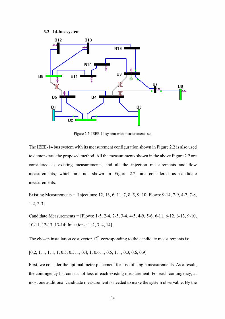
3.2 14-bus system

Figure 2.2 IEEE-14 system with measurements set

The IEEE-14 bus system with its measurement configuration shown in Figure 2.2 is also used

to demonstrate the proposed method. All the measurements shown in the above Figure 2.2 are

considered as existing measurements, and all the injection measurements and flow

measurements, which are not shown in Figure 2.2, are considered as candidate

measurements.

Existing Measurements = [Injections: 12, 13, 6, 11, 7, 8, 5, 9, 10; Flows: 9-14, 7-9, 4-7, 7-8,

1-2, 2-3].

Candidate Measurements = [Flows: 1-5, 2-4, 2-5, 3-4, 4-5, 4-9, 5-6, 6-11, 6-12, 6-13, 9-10,

10-11, 12-13, 13-14; Injections: 1, 2, 3, 4, 14].


[0.2, 1, 1, 1, 1, 1, 0.5, 0.5, 1, 0.4, 1, 0.6, 1, 0.5, 1, 1, 0.3, 0.6, 0.9]

First, we consider the optimal meter placement for loss of single measurements. As a result,

the contingency list consists of loss of each existing measurement. For each contingency, at

most one additional candidate measurement is needed to make the system observable. By the

35

method introduced in PART II, the candidate measurements, which are expressed as IP

problem constraints, can be obtained for each existing measurement loss:

1 :12. 19181716151413109754321 ≥++++++++++++++ xxxxxxxxxxxxxxxInj

1 :13. 19181716151413109754321 ≥++++++++++++++ xxxxxxxxxxxxxxxInj

1 :6. 18171615754321 ≥+++++++++ xxxxxxxxxxInj

1 :11. 191817161514131098754321 ≥+++++++++++++++ xxxxxxxxxxxxxxxxInj

1 :5. 181716154321 ≥+++++++ xxxxxxxxInj

1 :9.

1918171615

141312111098754321

≥+++++++++++++++++

xxxxxxxxxxxxxxxxxxInj

1 :10.

1918171615

1413121098754321

≥++++++++++++++++

xxxxxxxxxxxxxxxxxInj

1 :149

1918171615

141312111098754321

≥+++++++++++++++++−

xxxxxxxxxxxxxxxxxxFlow

1 :21 181716154321 ≥+++++++− xxxxxxxxFlow

1 :3-2 1817164 ≥+++ xxxxFlow

Finally, solution of the integer-programming problem yields the injection measurement at

bus-3 as the optimal choice that will ensure network observability under loss of any single

measurement at minimum cost 0.3. However, since we exclude the redundant existing

measurements in the candidate measurements, we decrease the complexity of the IP problem,

which is important for the IP solver.

Second, we consider the contingencies including loss of several measurements and outage of

single or several branches.

36

Contingency 1: loss of flow measurements in branch 1-2 and branch 2-3;

Contingency 2: loss of the injection measurement at bus 9, and loss of flow measurements in

branch 9-14 and branch 9-7;

Contingency 3: loss of injection measurement at bus 7, and loss of flow measurements in

branch 7-4 and branch 7-8;

Contingency 4: branch 10-11 outage; and

Contingency 5: branch 9-10 outage.

Besides the candidate measurements for the loss of single measurements, we also can obtain

the candidate measurement sets for these five pre-determined contingencies, which also are

expressed as IP constraints:

1:1 1634318217216242 ≥+×+×+×+×+×+× ΛxxxxxxxxxxxxContingecy

1:2 711511411311211111 ≥+×+×+×+×+×+× ΛxxxxxxxxxxxxContingecy

1 :3 8754321 ≥+++++++ ΛxxxxxxxyContingenc

1 :4 13109754321 ≥++++++++ ΛxxxxxxxxxyContingenc

1 :5 13109754321 ≥++++++++ ΛxxxxxxxxxyContingenc

In each contingency, for space limitation, not all sets of candidate measurements are listed

above. After considering these five pre-determined contingencies, the IP solver shows that

the optimal measurement set for this system is to include the injection measurement at bus 3

and the flow measurement in branch 1-5. Hence, inclusion of these additional measurements

will maintain the system observable during loss of any single measurement and these five

pre-determined contingencies in the IEEE-14 bus system.

37

3.3 30-bus system

Figure 2.3 IEEE-30 system with a measurements set

Existing Measurements = [Injections: 1, 2, 3, 5, 8, 9, 10, 12, 13, 15, 21, 24, 26, 27; Flows: 1-2,

1-3, 2-5, 2-6, 9-11, 12-13, 12-16, 14-15, 16-17, 15-18, 18-19, 10-21, 15-23, 22-24, 25-26,

25-27, 28-27, 29-30, 6-28].

Candidate Measurements = [Injections: 4, 6, 7, 11, 14, 16, 17, 18, 19, 20, 22, 23, 25, 28, 29,

30; Flows: 2-4, 3-4, 4-6, 5-7, 6-7, 6-8, 6-9, 6-10, 9-10, 4-12, 12-14, 12-15, 19-20, 10-17,

10-20, 10-22, 21-22, 23-24, 24-25, 27-29, 27-30, 8-28].


[0.4, 0.4, 0.6, 0.8, 0.8, 0.4, 0.4, 0.4, 0.6, 1, 2, 1, 0.6, 0.6, 0.6, 0.6, 0.2, 0.2, 2, 0.2, 0.2, 2, 0.4, 1,

0.4, 1, 0.4, 0.4, 1, 0.8, 0.8, 0.6, 2, 0.4, 0.4, 0.2, 1, 0.2]

38

Similar to the previous two example systems, we consider loss of any single measurement at

first. The corresponding IP constraints to loss of any single measurement are listed as

follows:

1 :Loss 5. 212032 ≥+++ xxxxInj

1 :Loss 8. 3822142 ≥+++ xxxxInj

1 :Loss 9. 312925231092 ≥++++++ xxxxxxxInj

1 :Loss 10. 3129109 ≥+++ xxxxInj

1 :Loss 12.

353431302926

2524231312109721

≥+++++++++++++++

xxxxxxxxxxxxxxxxInj

1 :Loss 15.

3534313029282726

25242313121097521

≥++++++++++++++++++

xxxxxxxxxxxxxxxxxxxInj

1 :Loss 21. 33323130292524231110972 ≥++++++++++++ xxxxxxxxxxxxxInj

1 :Loss 24.

35343130

29252423131210972

≥+++++++++++++

xxxxxxxxxxxxxxInj

1 :Loss 27. 37361615 ≥+++ xxxxInj

1:119 3129252310942 ≥+++++++− xxxxxxxxFlow

1:1612

3534313029262524

231313121097621

≥+++++++++++++++++−


1:1514

353431302928272625

242313121097521

≥++++++++++++++++++−xxxxxxxxxxxxxxxxxxxFlow

1:1716 31302910976 ≥++++++− xxxxxxxFlow

39

1:1815

353431302928272625

2423131210987521

≥+++++++++++++++++++−

xxxxxxxxxxxxxxxxxxxxFlow

1:1918 291098 ≥+++− xxxxFlow

1:2110

333231302925

24231110972

≥++++++++++++−xxxxxxxxxxxxxFlow

1:2422

35343130292425

2313121110972

≥++++++++++++++−

xxxxxxxxxxxxxxxFlow

1:2725

373635343331302925

24231615131210972

≥++++++++++++++++++−xxxxxxxxxxxxxxxxxxxFlow

1:2728

373635343331302925

2423161514131210972

≥+++++++++++++++++++−

xxxxxxxxxxxxxxxxxxxxFlow

1:3029 37361615 ≥+++− xxxxFlow

1:286

3835343331302925

24231214131210972

≥+++++++++++++++++−xxxxxxxxxxxxxxxxxxFlow

Compared with the A matrix in [2], obviously some injection measurement losses are not

listed here, such as loss of injection measurements at buses 1, 2, 3, 13, and 26. It is because

loss of any of above five measurements will not affect the network observability and no extra

measurement is needed.

Solving the IP problem as proposed, the optimal measurement set will be the injection

measurements at buses 6and 19, and the flow measurement in branch 27-29 with minimum

installation cost 1.2.

Next we include the other 5 contingencies into the contingency list besides loss of any single

measurement.

Contingency 1: loss of injection measurement at bus 1, and flow measurements in branches

1-2 and 1-3;

40


2-5 and 2-6; branches 1-2 and 2-4 are outaged;


12-13 and 12-16;

Contingency 4: loss of injection measurement at bus 26, and flow measurement in branch

25-26; and

Contingency 5: loss of flow measurement in branch 29-30; branch 27-30 is outaged.

As a result, for the given contingencies list, besides the candidate measurements for the loss

of single measurements, we also can obtain the candidate measurement sets for these five

contingencies, which also are expressed as IP constraints:

1 :1y Contingenc

1534313029252423

1918171312109721

≥++++++++++++++++++

xxxxxxxxxxxxxxxxxx

1 :2y Contingenc 12321032932732132 ≥∗∗+∗∗+∗∗+∗∗+∗∗ Λxxxxxxxxxxxxxxx

1 :3y Contingenc 3062961069676 ≥+∗+∗+∗+∗+∗ Λxxxxxxxxxx

1 :4y Contingenc 13 ≥x

1 :3y Contingenc 1615 ≥+ xx

The IP solver shows that the optimal measurement set for this system is to include the

injection measurements at buses 6, 19, 25, and 29, and the flow measurement in branch 5-7.

Hence, inclusion of these additional measurements will maintain the system observable

during loss of any single measurement and those five given contingencies in the IEEE-30 bus

system.

41

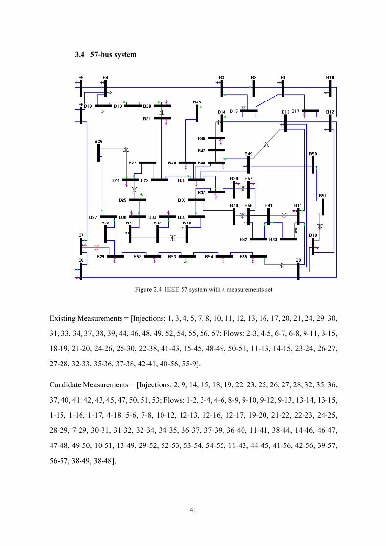
3.4 57-bus system

Figure 2.4 IEEE-57 system with a measurements set

Existing Measurements = [Injections: 1, 3, 4, 5, 7, 8, 10, 11, 12, 13, 16, 17, 20, 21, 24, 29, 30,

31, 33, 34, 37, 38, 39, 44, 46, 48, 49, 52, 54, 55, 56, 57; Flows: 2-3, 4-5, 6-7, 6-8, 9-11, 3-15,

18-19, 21-20, 24-26, 25-30, 22-38, 41-43, 15-45, 48-49, 50-51, 11-13, 14-15, 23-24, 26-27,

27-28, 32-33, 35-36, 37-38, 42-41, 40-56, 55-9].

Candidate Measurements = [Injections: 2, 9, 14, 15, 18, 19, 22, 23, 25, 26, 27, 28, 32, 35, 36,

37, 40, 41, 42, 43, 45, 47, 50, 51, 53; Flows: 1-2, 3-4, 4-6, 8-9, 9-10, 9-12, 9-13, 13-14, 13-15,

1-15, 1-16, 1-17, 4-18, 5-6, 7-8, 10-12, 12-13, 12-16, 12-17, 19-20, 21-22, 22-23, 24-25,

28-29, 7-29, 30-31, 31-32, 32-34, 34-35, 36-37, 37-39, 36-40, 11-41, 38-44, 14-46, 46-47,

47-48, 49-50, 10-51, 13-49, 29-52, 52-53, 53-54, 54-55, 11-43, 44-45, 41-56, 42-56, 39-57,

56-57, 38-49, 38-48].

42

The chosen installation cost vector TC corresponding to the candidate measurements is set

equal to 0.1.

First, we consider the loss of any single measurement. After obtaining all the IP constraints

corresponding to the loss of any single measurement, the optimal measurement set will be the

injection measurements at buses 14 and 32, with minimum installation cost of 0.2.

The corresponding IP constraints to loss of any single measurement are listed as follows:

1 :Loss 29. 5453494715141398 ≥++++++++ xxxxxxxxxInj

1 :Loss 7.

676654535049

472515141398

≥++++++++++++

xxxxxxxxxxxxxInj

1 :Loss 24. 545348151410 ≥+++++ xxxxxxInj

1 :Loss 30. 545352511514 ≥+++++ xxxxxxInj

1 :Loss 31. 5453521514 ≥++++ xxxxxInj

1 :Loss 34. 54531514 ≥+++ xxxxInj

1 :Loss 29. 5453494715141398 ≥++++++++ xxxxxxxxxInj

1 :Loss 37. 5755545317161514 ≥+++++++ xxxxxxxxInj

1 :Loss 39.

7574737257565554

53191817161514

≥++++++++++++++

xxxxxxxxxxxxxxxInj

1 :Loss 46. 6160224 ≥+++ xxxxInj

1 :Loss 48. 626160224 ≥++++ xxxxxInj

1 :Loss 52.

6766545349

472515141398

≥+++++++++++xxxxx

xxxxxxxInj

43

1 :Loss 54.

686766545349

472515141398

≥++++++++++++

xxxxxxxxxxxxxInj

1 :Loss 55.

69686766545349

472515141398

≥+++++++++++++

xxxxxxxxxxxxxxInj

1 :Loss 56.

7574737257565554

53191817161514

≥++++++++++++++

xxxxxxxxxxxxxxxInj

1 :32

7574737257565554

53191817161514

≥++++++++++++++−

xxxxxxxxxxxxxxxFlow

1 :2624 545348471514111098 ≥+++++++++− xxxxxxxxxxFlow

1 :3025 54535251151410 ≥++++++− xxxxxxxFlow

1 :4341

75747372705857565554

5320191817161514

≥+++++++++++++++++−


1 :2423 5453484715141098 ≥++++++++− xxxxxxxxxFlow

1 :2726 5453471514121198 ≥++++++++− xxxxxxxxxFlow

1 :2827 5453471514131298 ≥++++++++− xxxxxxxxxFlow

1:3635 5453161514 ≥++++− xxxxxFlow

1 :4142

7574737257565554

53191817161514

≥++++++++++++++−

xxxxxxxxxxxxxxxFlow

1 :5640

7574737257565554

53191817161514

≥++++++++++++++−

xxxxxxxxxxxxxxxFlow

1 :955

6968676654534947

25151413983

≥++++++++++++++−

xxxxxxxxxxxxxxxFlow

44

Next, we include the other 5 contingencies into the contingency list besides the loss of any

single measurement and outage of any single branch.

Contingency 1: loss of injection measurements at bus 4, and flow measurements in branches

4-5;

Contingency 2: loss of injection measurements at bus 24, and flow measurements in branches

23-24 and 24-26;


48-49; branch 38-48 is outage;

Contingency 4: loss of injection measurement at bus 37, and flow measurement in branch

37-38; branch 36-37 is outage; and

Contingency 5: loss of injection measurement at bus 3, loss of flow measurement in branches

2-3, 3-15; branch 3-4 is outage.

As a result, for the given contingency list, besides the candidate measurements for the loss of

single measurements and single branches, we also can obtain the candidate measurement sets

for these five contingencies, which are expressed as the following IP constraints:

Contingency 1: 1 16151498654321 ≥+++++++++++ Λxxxxxxxxxxx

Contingency 2: 14898159814981098 ≥+∗∗+∗∗+∗∗+∗∗ Λxxxxxxxxxxxx

Contingency 3: 1 626160224 ≥++++ xxxxx

Contingency 4: 1 57545317161514 ≥++++++++ xxxxxxx

Contingency 5: 1 221211514131 ≥+∗+∗+∗+∗+∗ Λxxxxxxxxxx

The IP solver shows that the optimal measurement set for this system is to include the

injection measurements at buses 2, 22, and 23, and the flow measurements in branches 34-35

and 46-47. Hence, inclusion of these additional measurements will maintain the system

45

observable during any single line outage or loss of any single measurement and those five

contingencies considered for the IEEE-57 bus system.

3.5 Conclusions

This part of the report presents several improvements to the unified measurement placement

method by considering the loss of multiple measurements and/or multiple branch outages.

Based on the modified measurement Jacobian H matrix for each contingency, a general

candidate measurements selection method is introduced so that all candidates can be selected

for loss of either single measurement and single branch or multiple measurements and

multiple branches. Furthermore, the integer programming problem is extended to those cases

where two or more candidates should be considered for placement due to a multiple

contingency. Numerical examples verify the effectiveness of the proposed method for meter

placement.

REFERENCES

[1] A. Abur and F.H. Magnago, “Optimal Meter Placement for Maintaining Observability During

Single Branch Outages”, IEEE Trans. On Power Systems, Vol. 14, No. 4, Nov. 1999, pp:

1273-1278.

[2] F.H. Magnago and A. Abur, “A Unified Approach to Robust Meter Placement Against Loss

of Measurements and Branch Outages”, IEEE Trans. On Systems, Vol. 15, 2000.

46

PART III: DESIGN OF DATA EXCHANGE ON DISTRIBUTED

MULTI-UTILITY OPERATIONS

I. INTRODUCTION

State estimation is essential for monitoring and control of a power system. In the historical

regulated environment, the power system was owned and operated by local utilities using their

own control area with a large amount of local generation to meet operational requirements.

These utilities had the responsibility for and the ownership of the instrumentation in their local

region to meet their needs for monitoring and control. There was little need to exchange

extensive amounts of data with other organizations.

In recent years, those utilities have been releasing operational control of their transmission grids

to form ISOs/RTOs while maintaining their own state estimators over their own areas [1]. In

addition, a recent trend for these ISOs/RTOs is to further cooperate and facilitate a power market

on as a Mega-RTO for better market efficiency [2]. The grid size of a Mega-RTO becomes

extremely large, as concluded recently by the Federal Energy Regulatory Commission (FERC)

that only four Mega-RTOs should cover the entire nation besides Texas [2].

many new problems ing achieving reliable state estimation arise under such an operating

environment. First, state estimation over the whole grid of a Mega-RTO becomes very

challenging because of its size. One possible scheme is to implement a new estimator over the

whole grid, named as one state estimation scheme (OSE), which has many disadvantages in the

aspects of investment and computation performance [3]. Recently, we developed a new

concurrent non-recursive textured algorithm as an alternative [3], where the currently existing

state estimators are fully utilized without using a new estimator. Such a distributed state

estimation (DSE) algorithm evolves from the original well-developed textured algorithm in [4]

with further distributed computations. The scheme also overcomes the disadvantages of OSE,

and the additional cost in DSE is only some extra communication for some instrumentation or

estimated data exchanges. In this part, the new issue is how to exchange instrumentation or

estimated data with neighboring entities in a power market. This leads to three notes.

47

1) Data exchange design is critical to the newly developed textured distributed state estimation

algorithm [3], which will be discussed in detail in the next part of the report.

2) Selected data exchange improves the quality of estimators in individual entities on both

estimation reliability and estimation accuracy. In this report ‘estimation reliability’ refers to bad

data detection and identification capability and probability to maintain observability under

measurement loss.

3) After the introduction of data exchange, the traditional measurement placement methodology

will be modified to fully utilize the benefit of data exchange.

Not all data exchanges are necessarily beneficial. In fact, some data exchange may harm the

local estimators and thus the exchange has to be carefully designed. Experience alone cannot

resolve the design issues. In particular, for big Mega-RTOs, no one has any experience yet.

Therefore, it is critical to develop a systematic approach to search for appropriate data exchange

schemes. Since the computation complexity increases dramatically for large grids, data

exchange design problem become very challenging.

Instrumentation/estimation data exchange issues in power market are discussed in [5]. Further

studies are given in [6], where a new concept of Bus Redundancy Descriptor (BRD) is

developed and utilized.

In this part, a knowledge-based system is proposed to efficiently search for beneficial data

exchange scheme, and the additional new features include the following:

1) Based on BRD in [6], a new concept of Bus Credibility Index (BCI) is proposed, where the

probability of good measurements is taken into account. Both BRD and BCI form the basis of

the knowledge and BCI is a probability measure that quantifies the estimation reliability.

2) The improvement of estimation accuracy is discussed.

3) The economic factor on the implementation of data exchange is considered. Activities used to

improve the quality of state estimation, including data exchange among member companies, are

market-based and the economic cost must be taken into account.

48

4) The impact of the data exchange on traditional measurement placement methodology is

discussed.

This part of the report is organized as follows. The concept of Bus Credibility Index (BCI) is

discussed in Section II. The knowledge base of the expert system is described in Section III.

Furthermore, in Section IV, the reasoning machine with the corresponding principles based on

BCI is discussed. Numerical tests are studied in Section V. In the last section, a conclusion is

drawn.

II. BUS CREDIBILITY INDEX (BCI)

A sample system S in Fig.1 is used in this section to explain our newly developed concept.

2.1 Basic analysis of state estimation

SE problem is based on the model [7]:

( )z h x e= +

where

z represents measurements,

Fig. 1 A Sample System S

power flow measurement

injection measurement

49

e is the measurement noise vector,

x is the state vector composed of the phase angles and the magnitudes of the voltages on

network buses, and

( )h • stands for the nonlinear measurement functions.

WLS algorithm has been used to solve the SE problem in many commercial software packages

for electric power system, which is based on a nonlinear iteration method. At each iteration i ,

the following equations is solved:

1 1 1 1 1( )T T Ti i ix H R H H R z G H R z− − − − −∆ = ∆ = ∆

where

R is the measurement covariance matrix,

H is the Jacobian matrix h x∂ ∂ , and

1TG H R H−= is the gain matrix.

2.2 Critical p-tuples

Critical p-tuples is first proposed in [8,9], and it is defined as a set of p measurements with

respect to a specific system, where the removals of all the p measurements in the set will make

the originally observable system unobservable. In addition, removals of any (p-1) measurements

in the set will still keep the system observable.

The size of the critical p-tuples is defined as p. Critical p-tuples can be determined based on the

analysis of symbolic Jacobian matrix H [10]. For example, the methodology in [11] can be used

to determine the critical tuples. For the sample system S, 9-10, 10,and 12-13 are a critical

3-tuple, which is denoted as (9-10,10,12-13|S).

Note: “10” stands for the pair of active and reactive power injection measurement in bus 10,

while “9-10” stands for the pair of the active and inactive power flow injection measurements

from bus 9 to bus 10.

50

2.3 Weak Bus Sets of Critical p-tuples

The weak bus set of a critical p-tuples is determined as:

Step1: Remove all the p measurements in the critical p-tuples, and S becomes unobservable

now.

Step2: Mark those lines with power flow measurements.

Step3: Select an unmarked line; if all the lines have been marked, stop and exit.

Step4: Add a pair of active and reactive flow measurements to this line for the time being and

mark the line.

Step5: If S turns to be observable again, then the buses located on the two ends of this line belong

to the Weak Bus Set of the critical p-tuples.

Step6: Remove the flow measurements just added in Step4, and go back to Step3.

For example, after the removal of (9-10, 10, 12-13|S), S becomes unobservable. If a pair of

active and reactive flow measurements is added on line 6-13, the system becomes observable

again. Therefore, buses 6 and 13 belong to the Weak Bus Set of (9-10, 10, 12-13|S). In fact, the

Weak Bus Set of (9-10, 10, 12-13|S) is bus 6, 9, 10, 12 and 13, which is denoted as {6, 9, 10, 12,

13|(9-10,10,12-13)|S }.

2.4 Bus Redundancy Descriptor (BRD)

Every bus has its own Bus Redundancy Descriptor (BRD) with respect to a specific system.

BRD of bus b is defined in [6] as a set of critical measurement p-tuples whose weak bus set

includes bus b.

A bus is said to have a bus redundancy level g, if the smallest size of the critical tuples in its BRD

is (g+1).

For example, it is determined in [6] that:

BRD(5,S)={(5-6), (1-5,5-1), …};

BRD(6,S)={(5-6), (6-11,6-12), (6-11,12-13), (6-12,12-13), (9-10,10,12-13), …};

51

BRD(11,S)={(6-11,6-12), (6-11,12-13), …};

BRD(13,S)={(6-11,6-12) (6-11,12-13) (6-12,12-13), (9-10,10,12-13), …}.

Note: BRD(13,S)={(6-11,6-12) (6-11,12-13) (6-12,12-13), (9-10,10,12-13), …} denotes BRD

of bus13 with respect to S consists of three critical pairs (6-11,6-12), (6-11,12-13) and

(6-12,12-13), a critical 3-triples (9-10,10,12-13), and other possible critical 4-tuples.

2.5 A new concept of Bus Credibility Index (BCI)

Bus Credibility Index of bus b is defined as the state estimation credibility probability on bus b

with respect to a specified system. BCI can be determined as:

1 2( , ) 1 ( )kBCI b S P C C C= − ∪ ∪⋅⋅⋅∪

11 2

1 1 1 2

1 ( 1) ( )k

it t ti

i t t ti k

P C C C−

= ≤ < <⋅⋅⋅< ≤

= − − ∩ ∩⋅⋅⋅∩

∑ ∑

∑∑≤<≤≤≤

∩−−=ktt

ttkt

t CCPCP211

2111

1 )()((1

1 2 31 1 2 3

( )t t tt t t k

P C C C≤ < < ≤

+ ∩ ∩ −⋅⋅⋅∑ )11 2( 1) ( )k

kP C C C−+ − ∩ ∩⋅⋅⋅∩ (1)

where

BCI(b,S) is the BCI of bus b with respect to system S;

BCD(b,S) consists of k critical p-tuples Ci, p=1,2,3,…;

( )iP C Cj∩ stands for the failure probability when all measurements in Ci and Cj fail.

If the failure probabilities of measurements are independent from each other, then ( )iP C Cj∩

can be determined by:

1 2( ) ( { , , , } )i lP C Cj P M M M=∩ ⋅⋅⋅ 1 2( ) ( ) ( )lP M P M P M= ⋅ ⋅⋅⋅ (2)

where

{M1, M2, …, Ml} are the measurement set which makes up ( )iC Cj∩ ,

52

P(Ml) stands for the failure probability of Ml.

Given the failure probability of every measurement, BCI(b,S) can be determined according to

equations (1) and (2).

For example, suppose the failure probability is fixed to 0.01, BCI(b,S) is determined as Table 1:

Table 1 BCI of Buses With Respect to Sample System in Fig. 1

BCI(5,S) BCI(11,S) BCI(13,S)

0.9900 0.9998 0.9997 2.6 Remarks

● The meaning of BCI depends on the definition of failure probability. If the failure probability

of measurements stands for the probability of measurement availability, then BCI(b,S) stands for

the probability to maintain observability on bus b with respect to system S since the removal of

all measurements of a critical k-tuples will make S unobservable. If the failure probability of a

measurement stands for the probability of bad data in this measurement, then BCI(b,S) reflects

the probability to successfully identify bad data since bad data cannot be identified if all the

measurements of a critical k-tuples are bad data. Therefore, BCI is a probability measure that

quantifies the estimation reliability on bus b with respect to a specific system S.

● Remark 2: If BCI(b1,S1)>BCI(b2,S2), then bus b1 with respect to system S1 is said to be

stronger than bus b2 with respect to system S2.

Note that data exchanges modify the original system S to S’, and the incremental difference of

BCI from (b,S) to (b,S’) stands for the benefit of such a data exchange on bus b in the sense of

estimation reliability.

● As pointed out in [6], a critical k-tuples not necessarily constitutes a connected measurement

area, and the weak bus set of a critical tuples is also not limited to the buses linked directly to the

measurements of the critical tuples.

The measurements in BRD(b,S) either connect directly with b or locates on a loop that includes

b. For example, BRD(b5,S) consists of (5-6 ) and (1-5,5-1) which connect directly with b5, and

53

BRD(b13,S) consists of critical tuples such as (6-11,6-12), (6-11,12-13), (6-12,12-13) and

(9-10,10,12-13), which are all located in the loop b6 b12 b13 b14 b9 b10 b11 b6.

● Given the condition that the failure probability of every measurement is very low (<0.01), then

the failure probability of the critical k-tuples where k is large enough can be ignored in the

computation of BCI. For example, 0000.1),( ≈SbBCI if the redundancy level of b with

respect to S is greater than 3, and only buses with redundancy level less than 4 are potential weak

parts of the system, which we should focus on.

● With the full consideration of measurement failure probability, BCI(b,S) is a more accurate

criterion to evaluate the estimation reliability compared with local or global bus redundancy

level.

III. KNOWLEDGE BASE

The knowledge base of the proposed expert system consists of the following parts.

1. Raw Facts

Raw facts refer to the data input directly by the user, such as:

1) The configuration, parameters and ownership of current power system network and

measurement system;

2) The failure probability and accuracy of measurements; and

3) The cost of instrumentation and estimated data exchange.

Importance of raw facts is rather clear. However, the knowledge is too primitive to be

informative. Therefore, more refined information, such as the BCI information and the

estimation accuracy information, must be extracted by an expert system based on the raw facts.

2. BCI Information

BCI(b, S) reflects the estimation reliability on bus b with respect to a specific system S, which is

very useful in data exchange design.

54

3. Variance of SE errors

It is well known [12] that the variances of the SE errors stand for the accuracy of SE.

Statistically, they represent the “squared distances” of the estimates from their true values. The

smaller the variances are, the better the SE solution is typically.

The state estimation error variances are the diagonal elements of matrix 1C G−= .

Since the error variances are only slighted influenced by the operation point, the comparison of

different data exchange scheme is executed on a uniform given operation point.

IV. REASONING MACHINE

An IEEE-14 bus system as shown in Fig. 2 is used to illustrate how the reasoning machine

works, where RTO-A and RTO-B will merge into one Mega-RTO. There are two existing local

estimators for systems A and B, where neither overlapping areas nor data exchange is involved.

Tthe algorithm and principles are not limited to the selected examples; they are applicable to all

systems.

We have explored ways in [3] to design a distributed state estimator from the existing estimators

instead of building a totally new estimator for the whole system. In this part, the design of data

exchange scheme is the focus. Data exchange is a prerequisite for the algorithm in [3]; when

properly designed, it will be beneficial to local estimators.

RTO B

Fig. 2 Two RTOs merge into one Mega-RTO

RTO A

55

A measurement system can be evaluated through different criteria, among which the most

important criterion is estimation reliability and estimation accuracy. As discussed before,

‘estimation reliability’ refers to bad data detection and identification capability and probability to

maintain observability under measurement loss, which is evaluated by BCI. Therefore, in the

following algorithm, we focus on only BCI instead of estimation reliability.

The processes in the reasoning machine are given below.

Step 1: Determine the maximum possible benefit on BCI after data exchange by:

( , ) ( , )A ABCI b Whole BCI b A− and ( , ) ( , )B BBCI b Whole BCI b B−

where bA are the boundary buses in A, such as b1,b5,b10,b14;

bB are the boundary buses in B, such as b2,b4,b9;

Whole stands for the whole system of Mega-RTO.

Only boundary buses are of concern because, in most cases, BCI of internal buses also improves

when BCI of boundary buses improve, although the rate is much smaller.

Step 2: If the maximum possible benefit of a boundary bus is less than a pre-defined threshold,

then this boundary bus will be ignored during the following searching process.

Step 3: For a given boundary bus { }A Bb b b∈ ∪ , some rules are used to search for beneficial data

exchange:

Rule 1 for Instrumentation Data Exchange:

For boundary bus bA in A, instrumentation data exchange should extend to boundary bus bB in B

given the condition ( , ) ( , )B ABCI b Whole BCI b A> . For example, it is reasonable for b2 and b4

in B to extends to include b1 and b5 in A, while it does not follow the principle that b9 in B

extends to include b10 or b14 in A.

56

Rule 2 for Instrumentation Data Exchange:

The final configuration after data exchange should avoid forming a radial structure; instead, a

loop is preferred. For example, branch b1-b5 and b5-b2 should also be included in B after data

exchange to avoid radial branch b2-b1 and b4-b5. On the other hand, b9 in B extend only to b10

in A will form a new radial branch b9-b10, which violates this principle.

Rule for Estimation Data Exchange:

Step 1: If ( , ) ( , )BCI b A BCI b B> where b is in the common part of A and B, then estimation

result exchange from A to B on this bus will improve ( , )BCI b B to the magnitude of

( , )BCI b A .

Estimation accuracy information is not used here because BCI is more important than estimation

accuracy in industry applications. Furthermore, in most cases, estimation accuracy improves

when BCI improves.

Step 2: System A and B are modified accordingly based on the newly found data exchange from

Step 1. BCI, estimation accuracy and the economic cost are evaluated on the ‘new’ system A and

B to verify the benefit.

Step 3: If BCI on the given bus b of the post-data-exchange system are close enough to that in

the whole system, then we can stop searching for new data exchange for bus b. Otherwise new

data exchange can be searched further.

Step 4: Step 3 is repeated on all boundary buses of A and B.

Under power market environment, economic factors are especially important and are considered

in the reasoning machine I the following ways.

1) The benefit of different data exchange schemes may differ greatly. The benefit may saturate

after some data exchange, which implies no major benefit can be obtained for more data

exchange.

57

2) The hardware/software cost on data exchange implementation should be minimized given the

condition that the performance is satisfied. In other words, even if scheme D1 is slightly better

than scheme D2 in performance, but it is still possible for industry to select D1 when D1 is much

more economical than D2.

3) The price tag of a data reflects not only the installation cost but also its market value. It is

possible for system A to attach a rather high price tag to a measurement that is especially useful

to system B. The proposed expert system is critical for the companies to determine the market

price based on the benefit of data exchange.

4) Since new measurements can be sold to other companies, the data exchange will have some

impact on measurement placement decision. Accordingly, the proposed expert system is useful

for both the design of the data exchange scheme and the new measurement placement decision.

58

Fig.3 Original System of B before data exchange

Fig.4 Modified System of B after data exchange

Data Exchange

Fig.5 Local estimators after instrumentation data exchange

Estimator A

Estimator B Data Exchange

59

V. NUMERICAL TESTS

The following cases demonstrate several points.

1. Not all data exchange is beneficial. In fact, some data exchange may harm the local estimators

in both estimation reliability and estimation accuracy.

2. With a few data exchanges, both estimation reliability and estimation accuracy of local

estimators can be improved to the level as high as that of the one estimator on whole system.

3. The data exchange has an impact on traditional new measurement placement approach.

Estimation reliability is evaluated via BCI.

5.1 Case 1: Harmful Data Exchange Scheme

RTO B with a data exchange scheme is given in Fig. 4 and the original system before data

exchange is given in Fig. 3. As mentioned before, such a data exchange does not follow our

principles. In fact this data exchange scheme is harmful for Company B, which is demonstrated

in the following way.

The comparison between original B and modified B is given as follows (given the bad data

probability of any measurement is 0.1, and the accuracy of any measurement is 0.01 p.u.):

Table 2 Average BCI On The Buses Of Company B

B in Fig. 3 B in Fig. 4 B in Fig. 5 Whole System 0.9647 0.9643 0.9662 0.9662

Table 3 Average Estimation Error On The Buses Of Company B

B in Fig. 3 B in Fig. 4 B in Fig. 5 Whole System 7.7314e-007 8.1738e-007 2.6471e-007 2.6326e-007

60

Table 4. Normalized Residues for Local Estimator B

Estimator B in Fig. 3 Estimator B in Fig. 4 Iteration No. Meas. Max. Residue Meas. Max. Residue 1st 9 164.72 9-4 89.41 2nd 9-7 108.05 7-4 56.78 3rd No bad data detected 4 34.68 4th N/A No bad data detected

Table 2 implies that the data exchange shown in Fig. 4 decreases B’s BCI, which means such a

data exchange scheme decreases estimation reliability. The following example demonstrate our

conclusion.

Suppose that both measurements, 9 and 9-7, are bad data in which the sign of these

measurements are reversed. When the measurement with largest normalized residue is removed

as bad data in WLS algorithm for SE, the SE is executed again to find other possible bad data.

Table 4 shows the result of such an iteration process. It is clear that before data exchange (Fig. 3)

these two bad data are detected, identified, and removed correctly while after data exchange

(Fig. 4) these bad data cannot be even detected at all.

The feature of this example is that even though the exchanged data are with no bad data, the

estimation reliability on local area is still seriously harmed after data exchange.

Table 3 indicates that B’s estimation error also increases after such a data exchange.

5.2 Case 2: Efficiency of Beneficial Data Exchange

Our expert system suggested an optimal data exchange scheme following our principles:

- Instrumentation data exchange: shown in Fig. 5.

- Estimation data exchange: Estimation result on bus 1 and 5 are exchanged from B to A. The

detailed algorithm to utilize these estimated data is given in detail in [3], which will be discussed

in the next part of the report.

Tables 2 and 3 compare the performances of distributed SEs and the whole system estimator. It

is clear that:

61

1) B in Fig. 5 improves the BCI over the buses belonging to original system in Fig. 3.

Furthermore, BCI for B shown in Fig. 5 is as good as the whole system estimation. It shows that

little benefit on BCI could be further gained through more data exchange.

2) B in Fig. 5 has improved its estimation accuracy over the original system in Fig. 3.

Furthermore, the accuracy difference between Fig. 5 and the whole system is rather small, which

shows that little benefit on estimation accuracy could be further gained through more data

exchange.

3) After data exchange, the local estimator achieves estimation reliability and estimation

accuracy as high as the one estimator for the whole system.

5.3 Case 3: Impact on New Measurement Placement (1)

Suppose the probability of accidents in the SCADA on station b1 is extremely high. Obviously,

such an accident would cause the voltage measurement on b1, power injection measurement on

bus1, power flow measurements 1-2 and 1-5 to all be unusable for the state estimation.

Accordingly, the system would become unobservable, which is unacceptable for RTO A.

From the traditional measurement placement viewpoint, in order to keep state estimation

running smoothly, at least one new measurement has to be installed, such as voltage

measurement on bus 5.

However, with data exchange, such a new measurement is not necessarily needed. When we

follow the data exchange scheme suggested in Case 2, the state estimation in RTO A can be run

normally even after the accident happened because the estimation result on b1 and b5 is

exchanged from B to A.

5.4 Case 4: Impact on New Measurement Placement (2)

Suppose that RTO A wants to improve the estimation accuracy on b5. From a traditional

measurement placement viewpoint, there are basically two alternatives: improve the accuracy

from original 0.01 to 0.001 on the measurement 5-1 or 5-6. These two alternatives have basically

the same effect to improve the estimation accuracy on b5.

62

On the other hand, if the accuracy of measurement 5-1 improves, the accuracy of RTO B also

improves if measurement 5-1 is exchanged from A to B. Therefore, it makes sense for RTO B to

share part of the cost with A to improve the accuracy of 5-1. Accordingly, it is better for A to

invest on measurement 5-1 instead of on measurement 5-6.

VI. CONCLUSION

In this part of the report, a knowledge-based system was proposed to search for beneficial

data exchanges for distributed state estimations. The knowledge includes the information on

Bus Credibility Index (BCI), which reflects the estimation reliability. The reasoning machine

consists of a few principles, where economic factors are also considered. Numerical tests on

IEEE-14 bus system demonstrate that properly selected data exchange improves the

estimator quality of all entities on both estimation reliability and accuracy. In addition, data

exchange has an impact on traditional measurement design. It was also shown that the

benefit of data exchange schemes can be quite different. Properly selected data exchanges

will enable the performance of the local distributed estimator to be as high as one estimator

on the whole system in both estimation reliability and estimation accuracy. On the other

hand, poorly designed data exchanges which do not follow our design rules may be harmful

to local estimators.

REFERENCES

[1] M. A. Lamoureux, “FERC’s Impact on Electric Utilities”, IEEE Power Engineering

Review, pp. 8-11, August 2001.

[2] Federal Energy Regulatory Commission, USA, Regional Transmission Organizations

Docket No. RT01-100-000, July 2001.

[3] Garng M. Huang and Jiansheng Lei, “A Concurrent Non-Recursive Textured Algorithm for

Distributed Multi-Utility State Estimation”, IEEE PES SM2002, July 2002.

63

[4] Garng M. Huang and S.- C. Hsieh, “Fast Textured Algorithms for Optimal Power Delivery

Problems in Deregulated Environments”, IEEE Trans. On Power Systems, Vol. 13, No. 2,

pp. 493-500, May 1998.

[5] Garng M. Huang and Jiansheng Lei, “Measurement Design and State Estimation for

Distributed Multi-Utility Operation”, North American Power Symposium 2001, pp.

504-509, October 2001.

[6] Garng M. Huang and Jiansheng Lei, “Measurement Design of Data Exchange for

Distributed Multi-Utility Operation”, IEEE PES WM2002, January 2002.

[7] F.C. Schweppe and E.J.Handschin, “Static state estimation in electric power systems,”

Proc. IEEE, Vol. 62, pp.972-982, July 1974.

[8] K. Clements, G. Krumpholz and P. Davis, “State Estimator Measurement System

Reliability Evaluation”, IEEE Trans. PAS, Vol. 101, pp. 997-1004, 1982.

[9] K. Clements, G. Krumpholz and P. Davis, “Power System State estimation with

measurement deficiency – An observability measurement placement algorithm”, IEEE

Trans. PAS, Vol. 102, pp. 2012-2020, 1983.

[10] I.W. Slutsker and J.M.Scudder, “Network observability analysis through measurement

Jacobian matrix reduction”, IEEE Transactions on Power Systems, Vol.2, No.2,

pp.331-337, May 1987.

[11] J. B. A. London, L. F. C. Alberto and N. G. Bretas, “Network observability: identification

of the measurements redundancy level”, Power System Technology, Proceedings 2000,

pp.577-582.

[12] M. K. Celik and W.-H.E. Liu, “An incremental measurement placement algorithm for state

estimation “, IEEE Trans. Power Systems , Vol.10, No.3 , pp.1698-1703, Aug. 1995.

64

PART IV: A CONCURRENT TEXTURED DISTRIBUTED STATE

ESTIMATION ALGORITHM

I. INTRODUCTION

As mentioned in part 3, power companies are releasing their transmission grids to form

ISOs/RTOs [1] while still maintaining their own local state estimators. In other words, companies

run their own SE’s and focus on the quality of SE in their own area. Therefore, there are multiple

state estimators distributed with different owners in one ISO/RTO. Furthermore, a recent trend for

these ISOs/RTOs is to further cooperate to run the power market on even a bigger grid, such as a

Mega-RTO, for a better market efficiency [2]. The grid of an ISO/RTO could be large. The size of

a Mega-RTO is even bigger, as concluded recently by Federal Energy Regulatory Commission

(FERC), that only four Mega-RTOs should cover the entire nation [2]. The state estimation over

the whole grid becomes very challenging just for its size.

One possible scheme is to implement a totally new estimator over the whole grid, and one state

estimator (OSE) is executed over the whole system. However, the OSE approach has many

disadvantages.

1) The investment in the new estimator could be enormous. The maintenance cost over such a

huge area is also high.

2) The size of the system is extremely large, which raises the scalability issue. The system matrix

becomes more ill-conditioned, and the computation speed and convergence performance becomes

slower and poorer.

3). The existing local state estimators distributed in different entities are wasted.

Because of the disadvantages of OSE, a new concurrent, non-recursive textured algorithm is

developed as an alternative to determine the state of the whole grid, where the currently existing

state estimators are fully utilized without using a new estimator. This textured algorithm is a

distributed state estimation (DSE) algorithm, which overcomes the disadvantages of OSE.

65

The concurrent textured algorithm has been well developed to deal with the optimization problem

of power systems by our team led by Dr. Huang [3, 4, 5]. The basic idea of a textured algorithm is

as follows [3]. First, the problem on a large system is decomposed into several smaller and more

tractable sub-problems for concurrent computation by fixing some boundary variables. Then, by

rotating the fixed variables, a recursive sequence of concurrent sub-problems are solved and the

original high dimension problem is solved by divide-and-conquer. The term ‘texture’ is because

there are overlapping areas between the neighboring sub-systems, which are just like texture. And

the boundary variables are located on these overlapping areas.

The introduction of such a concurrent textured algorithm into the state estimation problem avoids

the disadvantages of OSE. Furthermore, as compared with existing DSE algorithm [6,7,8], the

performance of the new algorithm improves greatly with respect to bad data detection and

identification ability, and to avoiding discrepancy on boundary buses.

The main flowchart and advantages of the new algorithm are discussed in Section II. The selection

of a data exchange scheme, as the center issue of the textured decomposition method, is described

in Section III. Furthermore, in Section IV, the sparse matrix technique and its application are

discussed. The determination of the state over the whole system is given in Section V. Numerical

tests are studied in Section VI. In the last section, Section VII, a conclusion is drawn.

66

II. CONCURRENT TEXTURED DSE ALGORITHM

2.1 Existing DSE Algorithms and their Drawbacks

Assume multiple entities such as companies, ISOs and RTOs, are connected physically and

cooperate to run the whole system as Fig. 1. Accordingly, there are multiple existing estimators

distributed in the sub-systems like Company A, Company B, ISO A, RTO A and RTO B. And

every entity maintains and executes their local state estimation on their own areas. These entities

are connected through tie lines near the boundary buses.

With the development of Information Technology (IT), DSE algorithms, especially those without

central controlling node [6, 7], become more and more applicable.

Company A

RTO BCompany B

RTO A

W hole System

ISO A forCompany A&B

Overlapping Areabetween RTO A

and RTO B

Overlapping Areabetween Co. A

and Co. B

Overlapping Areabetween Co. A

and RTO A

Fig. 2 Overlapping areas come into being after data exchange

Company A

RTO BCompany B

RTO A

W hole System

ISO A forCompany A&B

Fig. 1 Multiple Companies/ISOs/RTOs connected physically

67

The main drawback of the existing DSE algorithms [6,7,8] is that bad data detection and

identification ability decreases greatly compared to OSE which is over the whole system,

especially when bad data are close to the boundary of individual estimators. Moreover, the

estimation accuracy on boundary buses are much lower than OSE, which decrease the accuracy in

determination of the global reference bus and which make the whole result inconsistent.

2.2 Introduction of a New Algorithm

The objective of our new algorithm is to remove the drawback of existing DSE algorithm while

preserve the beneficial characteristics. In the new algorithm, there are some overlapping areas in

the neighboring estimators as shown in Fig. 2, where some information are shared.

Furthermore, the point here is to extend the sharing information; not only are the boundary buses

shared formally in the estimation sub-problems, as in [6], but also instrumentation data (real time

measurement information before execution of local estimator) and estimated data (estimation

results after execution of local estimator) are exchanged among neighboring entities. Such a data

exchange is introduced simultaneously between multiple entities, such as Company A and

Company B, ISO A and Company B, Company B and ROT B, and so on. Accordingly, a textured

network is formed.

2.3 Main Algorithm

The new algorithm is described as follows:

• Step1: Select a set of real time instrumentation data to be exchanged between neighboring

entities.

• Step2: Select a set of estimated data to be exchanged between neighboring entities.

• Step3: Taking the exchanged instrumentation data into account, the multiple local estimators

distributed in different entities are executed simultaneously and asynchronously until they

converge individually to the desired tolerance.

• Step 4: In view of the exchanged estimated data, modify the estimation result of local

estimators accordingly and re-run bad data analysis.

68

• Step5: Based on the modified results of local estimators, finally determine the state of the

whole system according to the different accuracy and reliability of estimators.

2.4 Advantages of the New Algorithm

● Advantage 1: Bad data detection and identification ability in the new algorithm is higher than

the existing DSE algorithm, especially when bad data appear close to the boundary of individual

estimators. Such an improvement is because of the cooperation between estimated data exchange

scheme and the textured network formed by instrumentation data exchange.

For example, in the existing DSE algorithm, if bad data appears in the boundary of one local

estimator A, then it is hard to be detected in A. However, in a textured decomposition

environment, the boundary buses in A are internal buses of another estimator (for example B) at

the same time, where the bad data can be detected. And the corrected information on these buses

will be exchanged from B to A via estimated data exchange, which will finally make A also

capable to detect the bad data. This capability suits well for an industrial environment in which it

is better to obtain SE results with good enough accuracy without bad data than the results with

higher accuracy, but with possible undetected bad data.

● Advantage 2: The estimation accuracy on boundary buses is much higher than existing DSE and

is comparable to OSE. Our approach decreases the discrepancy on the boundary buses and makes

the whole result more consistent.

● Advantage 3: Many earlier methods of DSE assume a star-like function network [8] where the

communications between the multiple remote processors and the central computer are critical

during iteration processes. Such a hierarchical approach suffers from bottleneck and reliability

issues because of the central controlling node. Our concurrent textured algorithm is asynchronous

without a central controlling node. As a consequence, the new algorithm becomes very fast and

practical.

● Advantage 4: Utilizing the instrumentation decoupling nature in SE, we removed the recursion

process in our original optimization. At the same time, the performance of estimation is still

69

satisfied, which is verified in our numerical tests. As a consequence, the speed of our new

algorithm gets even faster. This further advances our original textured algorithm.

● Advantage 5: The multiple local estimators can use different SE algorithms. Furthermore, the

convergence tolerance can be different based on different quality of local measurement systems.

Accordingly, our new algorithm becomes very flexible in which current existing estimators can be

included easily.

● Advantage 6: The performance of bad data detection and estimation accuracy in individual

existing estimators improves as well, which benefits individual companies/ISOs/RTOs.

Accordingly, they are more willing to share the information for their own benefits.

III. DSE TEXTURED DECOMPOSITION METHOD

3.1 Introduction

As discussed, we need to determine an instrumentation data and estimated data exchange scheme

to be used in Step 1 and Step 2. As special cases, if all the information is exchanged and shared,

the estimation becomes one estimator over the whole system, an OSE but not a DSE. On the other

hand, if no measurement is exchanged, it becomes the existing DSE algorithm, which has the

drawbacks described before. Therefore, a trade-off in the selection of data exchange is necessary

to make the overlapping areas moderate, not too large nor too small. Then, an appropriate texture

can be formed, which is a critical precondition for our new algorithm.

In addition, in the original textured decomposition method [3-5], the decomposition is based on

the requirements of the algorithm. However, in the DSE problem, the range of individual

estimators has been determined in advance from the actual industry ownership. And the

hardware/software cost on data exchange implementation should be minimized, which implies

schemes with smaller overlapping areas are preferred if all the other performance remains the

same.

Not all the data exchange is beneficial. In fact, some data exchange may harm the local estimators

and thus the exchange has to be carefully designed. Experience alone cannot resolve the design

issues. In particular, for big mega-RTOs, no one has any experience.

70

Therefore, it is critical to develop a systematic approach to search for appropriate data exchange

schemes, which can also help the design automation process.

3.2 A Systematic Textured Decomposition Method

Our effective data exchange scheme design method and the corresponding software have been

proposed to determine the textured decomposition by us in [9], which is discussed in the previous

part of the report. A simple description is given below.

The strength of bus b in estimator A is defined as the bad data detection and identification ability

and estimation accuracy on bus b in this particular estimator A. A newly developed concept of

Bus Redundancy Descriptor (BRD) is used to numerically evaluate the strength of every bus in

different estimators. Details of the definition of BRD and determination of strength are given in

[9].

Accordingly, two main rules are proposed by us [9] to search for the estimated

data/instrumentation exchange, which is a critical part of textured decomposition.

After data exchange, the strength of buses improves greatly. And the ultimate objective is that the

strength of every bus in the local estimators is almost as high as that in OSE. As for the buses in

the overlapping areas of different local estimators, the objective is to ensure that the strength of

these buses is high enough in at least one local estimator. The accomplishment of such an

objective is critical to obtaining the advantages 1 and 2 of the new algorithm.

In addition, artificial intelligence (AI) is widely used to deal with problems described with

uncertain terms like ‘almost’. Therefore, the application of AI to the textured decomposition

problem is quite natural.

3.3 Numerical Examples

Different distribution of local estimators will leads to different textured decomposition schemes.

For example, in an IEEE-14 bus system as shown in Fig. 3, RTO-A and RTO-B will merge into

one Mega-RTO. There are already two local estimators A and B, distributed in RTO A and RTO

B, with neither overlapping areas nor data exchange. In other words, no texture exists in the local

estimators.

71

A suggested textured decomposition is shown in Fig. 4.

Instrumentation Data Exchange:

Estimator A expands to include bus 9. Furthermore, the instrumentation data on these buses, such

as 9-10 (power flow measurements from bus 9 to bus 10), 9-14 and 9 (power injection

measurement on bus 9), are also exchanged from B to A in a real time manner. And estimator A is

executed in such an expanded sub-system.

Estimator A

Estimator B Data Exchange Area

Fig. 4 Local estimators after raw data exchange

RTO B

Fig. 3 Two RTOs merge into one Mega-RTO

RTO A

http://www.pserc.wisc.edu/../../../../../../WINDOWS/TEMP/Documents and Settings/b0x7826/Local Settings/Temp/[email protected]

72

Similarly, estimator B expands to include bus 1 and bus 5. Instrumentation data, such as 1-5 and

1-5, are also exchanged from A to B.

Therefore, the textured estimator consists of two independent estimators A and B with the

overlapping areas including buses 1, 2, and 9. However, estimated data exchange needs extra

updating as described below.

Estimated Data Exchange:

After local estimator A and B have been executed simultaneously and asynchronously, selected

estimation result in A, such as 9-14, 9-14 and 9, are exchanged from A to B. In view of these

estimated data, B modifies its own estimation result accordingly and re-runs the bad data analysis.

Similarly, selected estimation result in B, such as 1-5, 5-1 and 1, are exchanged from B to A.

Taking these estimated data into account, A also modifies its own estimation result accordingly

and re-runs the bad data analysis.

IV. ESTIMATED DATE EXCHANGE

4.1 Sparse Technique for Matrix Modification

Sparse technique for matrix modification is widely used in power system computation, and the

main idea isthat instead of re-computing a new sparse matrix, a modification on the old one is

processed to reduce its computation complexity. One major technique about the inverse matrix of

sparse matrix (A+MaNT) is well known as:

1 1( )TA MaN A− −+ = 1 1 1 1 1( )T TA M a N A M N A− − − − −− + (1)

where A is a n n× high-dimension sparse square matrix whose inverse matrix 1A− is already

computed in advance, and

a is a m m× square matrix and m is much less than n.

The computation complexity of re-computing 1( )TA MaN −+ is much higher than that of right

side of (1).

73

4.2 Application of the Sparse Technique

In Step 4 of the flowchart, after the estimated data exchange, the succeeding modification on the

estimation result of local estimators can be time-consuming if local estimation is executed again

from the very beginning. When a sequential SE algorithm, such as orthogonal method based on

row-wise Givens rotations [10], is used in local estimator, the speed of such a modification

process is fast even without other special techniques because of the nature of the sequential SE

algorithm. However, if the conventional Gauss Newton method is utilized in local estimator, it is

time-consuming to execute SE again. Therefore, a sparse matrix modification technique is

developed to modify the estimation result of local estimators and to avoid re-computing from the

very beginning when some estimated data are newly added from other neighboring estimators.

Such a technique can significantly accelerate the process in Step 4. Details are discussed below.

As described in Part III, section 2, the SE problem is based on the model [11]:

( )z h x e= + (2)

where

z represents measurements,

e is the measurement noise vector,

x is the state vector composed of the phase angles and the magnitudes of the voltages on network

buses, and

( )h • stands for the nonlinear measurement functions.

Traditionally a nonlinear iterative algorithm is widely used to solve the SE problem. At each

iteration i , the following equations is solved:

1 1 1 1 1( )T T Ti i ix H R H H R z G H R z− − − − −∆ = ∆ = ∆ (3)

where

R is the measurement covariance matrix

74

H is the Jacobian matrix h x∂ ∂ ,

1i i ix x x+∆ = − ,

( )i iz z h x∆ = − ,

1TG H R H−= is the gain matrix.

The most time-consuming computation in solving (3) is the determination of G and 1G− .

Suppose SE result based on current measurements is already obtained, and then some new data

are introduced while the observable island maintains same, that is, the dimension of state variables

is fixed.

Then the following equations hold:

( )( )new new new

z h x ez h x e

= + ⇒

11

1

00

T Ti new

newnew

HRx H H

HR

−−

−

∆ = •

1

1

00

T Tnew

newnew

zRH H

zR

−

−

∆ ∆

( ) 11 1 1( )T T Tnew new new new new newG H R H H R z H R z

−− − −= + ∆ + ∆ (4)

where the subscript ‘new’ stands for the newly introduced exchanged estimated data, whose

dimension is very low.

Since the new measurements in Step 4 are estimated data with high accuracy, it is reasonable to fix

H as a constant during modification process. Therefore, 1( )TH R z− ∆ and 1G− in (4) are the same

as those in the old SE result (3), and they are known before modification process.

Accordingly, considering the dimension of Rnew is much lower than that of G, sparse matrix

technique described in (1) can be utilized here to determine ( ) 11Tnew new newG H R H

−−+ in (4).

Consequently, the modification is no longer time-consuming.

75

V. DETERMINATION OF STATE OVER WHOLE GRID

After the first four steps of the flowchart have been executed, the state over whole grid is

determined as follows.

Step 5.1: Determine the angle difference of reference buses between any two local estimators. A

reasonable scheme is based on the estimation accuracy of different local estimators, and the

scheme is formulated as:

1 1 1 1, , , , , ,( )( ) ( )AB i A i B i A i B i A i B

i I i Ic c c cθ θ θ − − − −

∈ ∈

∆ = − + +∑ ∑ (5)

where ABθ∆ is the angle difference of reference buses between local estimator A and B,

I is the set of all the overlapping buses of estimator A and B,

,i Aθ is the estimated angle on bus i in estimator A, and

,i Ac is the i-th diagonal element of covariance matrix 1−= GC .

Matrix C stands for the variances of estimation errors on bus i in estimator A. Therefore, the

magnitude of ,i Ac is proportional to the estimation error on bus i in estimator A.

Step 5.2: Select a reference bus of one estimator (e.g. A) as the global reference bus for the whole

grid.

Step 5.3: Determine the angle difference between this global reference bus and the reference bus

in every local estimator. For local estimators (e.g. B) that connect directly with A, (5) can give the

angle difference directly. However, for local estimators (e.g. C) that only connect the neighboring

estimators of A (e.g. B) while estimator C itself does not connect with A directly, then the

following equation is utilized:

AC AB BCθ θ θ∆ = ∆ + ∆ .

Step 5.4: The estimated angle of each local estimator will be subtracted with the angle difference

between the global reference bus and the local difference bus.

76

Step 5.5: For non-overlapping buses, the state variables are finally determined, which is just the

current estimation result in local estimators.

Step 5.6: For overlapping bus i belonging to multiple local estimators , 1, 2,...,jK j m= , the state

variables ix are finally determined as:

1 1, , ,

1 1

( )j j j

m m

i i K i K i Kj i

x x c c− −

= =

=∑ ∑

where , ji Kx is the state variable of bus i in estimator jK .

VI. NUMERICAL RESULTS

IEEE 14-bus system mentioned before is used to verify that:

1.The accuracy and discrepancy performance is satisfied compared to OSE, and higher than the

existing DSE algorithm; and

2.The bad data detection ability improves greatly than existing DSE algorithm where bad data

analysis is executed only in individual local estimators.

6.1 Case 1: Accuracy and Discrepancy

Suppose there is a deviation of 0.01 p.u. on power flow measurement 5-2, which is still in the

range of tolerance, and no bad data is detected. Table 1 shows concurrent textured DSE algorithm

is more accurate than existing DSE algorithm without data exchange.

Accordingly, the discrepancy decreases from 0.007 in existing DSE without data exchange to

0.004 in textured DSE.

Table 1 Estimation Result Derivation

Algorithm OSE Existing DSE without data exchange Textured DSE Deviation on

2θ 0.003 0.007 0.004

77

6.2 Case 2: Effect of textured instrumentation data exchange (1)

Bad Data in RTO A: Suppose that 11-10 is bad instrumentation data (where the sign is reversed).

Measurements with largest normalized residues will be selected as bad data according to WLS

algorithm for SE.

Without Instrumentation Data Exchange (Non-Textured):

For estimator A in Fig. 3, 11-10 can only be detected as bad data, but cannot be identified based on

Table 2.

With Instrumentation Data Exchange (Textured):

For estimator A in Fig. 4, 11-10 is identified successfully according to Table 2.

Table 2 Normalized Residues For Local Estimator A

Estimator A in Fig. 3 Estimator A in Fig. 4 Order

Meas. Max.Residue Meas. Residue

10 53.38660 11-10 52.40 1 11-10 53.38660 10 46.42

6.3 Case 3: Effect of textured instrumentation data exchange (2)

Bad Data in RTO B: Suppose that both 2-3 and 2-4 are bad data (all increase by 0.1 p.u.).

Without Instrumentation Data Exchange (Non-Textured):

For estimator B in Fig. 3, 2 and 4 are selected incorrectly as bad data based on Table 3.

With Instrumentation Data Exchange (Textured):

For estimator B in Fig .4, 2-4 and 2-3 are identified successfully one by one based on Table 3.

Table 3 Normalized Residues For Local Estimator B

Estimator B in Fig. 3 Estimator B in Fig. 4 Order Meas. Max. Residue Meas. Max. Residue 1 2 106.8 2-4 94.9 2 4 44.8 2-3 83.4

78

6.4 Case 4: Effect of estimated data exchange

Bad Data In RTO A: Suppose that both 1-5 and 5-1 are bad data (all increased by 0.1 p.u.).

Without Estimated Data Exchange:

Even for estimator A with instrumentation data exchange as shown in Fig. 4, 1 and 5 are still

selected incorrectly as bad data according to Table 4.

With Estimated Data Exchange:

Step 1) Estimator A in Fig. 4 with instrumentation data exchange is executed. By now 1 and 5 is

still identified incorrectly as bad data by A according to Table 4.

Step 2) Simultaneously, estimator B is executed with instrumentation data exchange as shown in

Fig. 4. Then, 1-5 and 5-1 are both identified as bad data successfully one by one based on Table 4.

Therefore, estimation results on 1-5 and 5-1 are corrected in estimator B.

Step 3) These corrected values on 1-5 and 5-1 are exchanged from B to A, which follows the

estimated data exchange scheme mentioned before. These values are treated in estimator A as

pseudo-measurements with particular high accuracy and reliability.

Step 4) Taking the new pseudo-measurements into account, estimator A modifies its own

estimation result and re-runs bad data analysis. This time, 1-5 and 5-1 are both successfully

identified as bad data in estimator A based on Table 4.

Table 4 Normalized Residues For Local Estimator A and B

Estimator A in Fig. 4 Estimator B in Fig. 4 Estimator A in Fig. 4 with estimated data exchange Order

Meas. Max. Residue Meas Max.

Residue Meas. Max. Residue

1 1 68.95 5-1 87 5-1 84

2 5 59.4 1-5 84 1-5 94

79

VII. CONCLUSIONS

As noted, there is a recent trend for ISOs/RTOs is to grow toward a Mega-RTO grid. Certainly,

the determination of state over the whole system becomes very challenging due to its size.

Instead of starting a totally new estimator over the whole grid, a distributed concurrent textured

algorithm is proposed to determine the state of whole grid, where the currently existing state

estimators distributed in different companies/ISOs/RTOs are fully utilized. The new algorithm is

based on extra communication for some instrumentation or estimated data exchange. In addition,

such an algorithm is non-recursive, asynchronous, and avoids a central-controlling node. Sparse

matrix techniques are also utilized when updating local estimation through estimated data

exchanges. Therefore, the new algorithm is fast and practical. Furthermore, based on the

developed textured decomposition method, numerical tests verify that the performance of the

new textured DSE algorithm greatly improves as compared to existing DSE algorithms, with

respect to bad data analysis, estimation accuracy and elimination of discrepancy on boundary

buses.

REFERENCES

[1] M. A. Lamoureux, “FERC’s Impact on Electric Utilities”, IEEE Power Engineering

Review, pp. 8-11, August 2001.

[2] Federal Energy Regulatory Commission, USA, Regional Transmission Organizations

Docket No. RT01-100-000, Issued July 12,2001.

[3] Garng M. Huang and S.-C. Hsieh, “Fast Textured Algorithms for Optimal Power Delivery

Problems in Deregulated Environments”, IEEE Trans. On Power Systems, Vol. 13, No. 2,

pp. 493-500, May 1998.

[4] J.Zaborszky, Garng M. Huang, and K. W. Lu, “A textured model for computationally

efficient reactive power control and management”, IEEE Trans. On Power Apparatus and

Systems, Vol. PAS-104, No. 7, pp. 1718-1727, July 1985.

80

[5] Garng M. Huang, and S.-C. Hsieh, “A parallel HAD-textured algorithm for constrained

economic dispatch control problems”, IEEE Trans. On Power Systems, Vol. 10, No. 3, pp.

1553-1558, August 1995.

[6] D.M. Falcao, F. F. Wu, and L. Murphy, “Parallel and Distributed State Estimation,” IEEE

Trans. On Power Systems, Vol. 10, No.2, pp. 724-730, May 1995.

[7] K A-Rahman, L. Mili, A. Phadke, J.D.L. Ree and Y. Liu, “Internet based wide area

information sharing and its roles in power system state estimation”, IEEE PES SM2001,

July, 2001.

[8] T. V. Cutsem and M. Ribbens-Pavella, “Critical Survey of Hierarchical Methods for State

Estimation of Electrical Power Systems,” IEEE Trans. On Power Apparatus and Systems,

Vol. 102, No.10, pp. 3415-3424, October 1983.



[10] Simoes-Costa and V.H.Quintana, “An orthogonal row processing algorithm for power

system sequential state estimation,” IEEE Trans. Power Apparatus and System, Vol.100,

pp.3791-3800, Aug.1981.

[11] F.C. Schweppe and E.J.Handschin, “Static state estimation in electric power systems,”

Proc. IEEE, Vol. 62, pp.972-982, July 1974.

81

PROJECT PUBLICATIONS [1] Garng M. Huang and Jiansheng Lei, “A Knowledge Based Data Exchange Design for

Distributed Mega-RTO Operations”, Probabilistic Methods Applied to Power Systems

2002, September 2002.

[2] Garng M. Huang and Jiansheng Lei, “A Concurrent Non-Recursive Textured Algorithm for

Distributed Multi-Utility State Estimation”, IEEE PES SM2002, July 2002.



[4] Garng M. Huang and Jiansheng Lei, “Measurement Design and State Estimation for

Distributed Multi-Utility Operation”, North American Power Symposium 2001, pp.

504-509, October 2001.

[5] Qifeng Ding and A. Abur, “An Improved Measurement Placement Method against

Loss of Multiple Measurements and Branches”, Proceedings of the IEEE PES Winter

Meeting, New York, NY, Jan. 2002.

82

PROJECT CONCLUSIONS This project has focused on issues related to state estimation in a new power market operating

environment. The first issue is the improvements needed in the measurement design in order to

ensure reliable state estimation even under contingency conditions. This is addressed by

developing a meter placement method which determines the least cost metering upgrade while

accounting for contingencies. Another issue is the incorporation of FACTS devices into the state

estimation formulation. This is accomplished by modifying the estimation problem formulation

and by including the operation and parameter limits of the FACTS devices. The issue of

distributed multi-utility operation is addressed by developing a distributed textured decomposition

state estimator and also by devising strategies for efficient measurement exchange between

utilities.

The results of the project are implemented with prototype software tested on typical power system

configurations.