Embed Size (px)
Citation preview

Power System Stability Analysis Using
Recursive Projection Method
Aysar Musa
Submitted to the
Institute of Graduate Studies and Research
in partial fulfillment of the requirements for the Degree of
Master of Science
in
Electrical and Electronic Engineering
Eastern Mediterranean University
January 2013
Gazimağusa, North Cyprus

2
Approval of the Institute of Graduate Studies and Research
Prof. Dr. Elvan Yılmaz
Director
I certify that this thesis satisfies the requirements as a thesis for the degree of Master of
Science in Electrical and Electronic Engineering.
Prof. Dr. Aykut Hocanın
Chair, Department of Electrical and Electronic Engineering
We certify that we have read this thesis and that in our opinion it is fully adequate in
scope and quality as a thesis for the degree of Master of Science in Electrical and
Electronic Engineering.
Prof. Dr. Osman Kükrer
Supervisor
Examining Committee
1. Prof. Dr. Osman Kükrer
2. Prof. Dr. Runyi Yu
3. Asst. Prof. Dr. Suna Bolat

iii
ABSTRACT
Stability represents significant criteria in power system operation. Stability analysis of
power systems has been done by using an efficient numerical technique that is the
recursive projection method (RPM). RPM analyzes the outputs of the time domain
simulation code (TDSC) that is used to simulate the dynamics of a power system, to
define a slow/unstable operating mode as a subspace of system’s full space and applying
Newton method to improve the convergence of system solution, while fixed-point
iteration method is used in the supplement subspace of stable modes. The analysis is
performed by detecting those eigenvalues of the state matrix with magnitudes greater
than unity, and creating the corresponding orthonormal basis that participates in
extending the solution's convergence. This leads to getting a more accurate and stable
solution in power systems. When a perturbation occurs to the power system, applying
RPM allows the numerical solution to reach its steady-state mode in a short time and
without continuous oscillation. Verification of RPM’s achievements has been performed
on an example of 6-bus power system. The environment of this work is the Matlab
program supported by the power system toolbox (PST).
Keywords: Power system analysis, recursive projection method, numerical integration
methods.

iv
ÖZ
Kararlılık güç sistemlerinin çalışması açısından önemli bir kriterdir. Bu çalışmada güç
sistemlerinin kararlılık çözümlemesi, özyineli izdüşüm yöntemi (RPM) denen etkili bir sayısal
yöntem kullanılarak yapılmıştır. RPM ilk önce güç sisteminin dinamiğinin benzetimi için
kullanılan zaman erim benzetim yazılımının çıktılarını analiz eder ve yavaş veya kararsız
çalışma kiplerini, sistem uzayının değişimsiz bir altuzayı olarak tanımlar. Bu değişimsiz altuzay
üzerinde Newton yöntemi uygulanıp çözümün yakınsaması iyileştirilir. Kararlı kiplere ait
tümleyen uzay üzerinde ise sabit-nokta dürümü uygulanmaya devam eder. Analiz, durum
matrisinin özdeğerlerinin bulunmsı ve bunlardan genliği birden büyük olanlara karşılık gelen ve
çözümün yakınsamasını sağlayacak olan tam dikgen temel oluşturarak yapılır. Bu yolla güç
sistemlerinin analizinde kararlı ve doğruluğu yüksek olan bir çözüm elde edilir. Güç sisteminde
bir hata oluştuğunda, RPM sayısal çözümün durağan duruma kısa zamanda ve salınımsız olarak
erişmesini sağlar. RPM’in başarımı 6 baralı bir sistem üzerinde denenerek
doğrulanmıştır.Çalışmalar Matlab ortamında, daha önce geliştirilmiş olan Güç Sistemleri Paketi
kullanılarak yapılmıştır.
Anahtar kelimeler: Güç sistemleri kararlılığı, Özyineli İzdüşüm Yöntemi, Sayısal Çözüm
Yöntemleri.

v
DEDICATION
This dissertation is dedicated to my beloved wife and my parents for their love, devoting
their time to support me. Further, I would like to dedicate this work to my uncle for his
encouragement and endless support.

vi
ACKNOWLEDGMENTS
Thank god for helping me and giving me the ability to complete my thesis. My deepest
thanks and appreciation go to my supervisor; Prof. Dr. Osman Kükrer who supported me
during my thesis, without him this work may not be possible.
I would like to thank the chairman of my department, Prof. Dr. Aykut Hocanın, advisor
Assoc.Prof. Dr. Hasan Demirel, and all the staff of Electrical and Electronic Engineering
Department for their guidance and support.
I would like to thank Eastern Mediterranean University for accepting me as a master
student, and giving me the opportunity to be a member of graduate students of EMU.
My deepest thanks and gratitude for Thesis Monitoring Committee members, Prof. Dr.
Osman Kükrer, Prof. Dr. Runyi Yu and Asst. Prof. Dr. Suna Bolat for their supervision
and guidance to discuss my thesis.

vii
TABLE OF CONTENTS
ABSTRACT ..................................................................................................................... iii
ÖZ ..................................................................................................................................... iv
DEDICATION ................................................................................................................... v
ACKNOWLEDGMENT ................................................................................................... vi
LIST OF TABLES ............................................................................................................ ix
LIST OF FIGURES ........................................................................................................... x
LIST OF SYMBOLS/ABBREVIATIONS ....................................................................... xi
1 INTRODUCTION .......................................................................................................... 1
2 STABILITY ANALYSIS OF POWER SYSTEM ......................................................... 9
2.1 Synchronous Machines ............................................................................................. 9
2.2 Swing Equation ...................................................................................................... 10
2.3 Swing Equation of Single Machine ........................................................................ 12
2.4 Power-Angle Relation ............................................................................................ 15
2.5 Equal-Area Criterion .............................................................................................. 15
2.6 Multi-Machine Power System ................................................................................ 18
2.7 Differential Algebraic Equations ............................................................................ 19
2.8 Modified Euler’s Method ....................................................................................... 21
3 RECURSIVE PROJECTION METHOD (RPM) ......................................................... 24
3.1 Definition of RPM .................................................................................................. 24
3.2 Basic Procedure of RPM ........................................................................................ 26
3.3Computational Properties ........................................................................................ 28

viii
4 SIMULATIONS AND RESULTS ................................................................................ 30
4.1 Case Study .............................................................................................................. 31
4.2 Transient Stability Simulation Using ode23 Solver ............................................... 32
4.3 Application of Modified Euler Method .................................................................. 36
4.4 Finding the Jacobian Matrix ................................................................................... 37
4.5 Transient Sability Simulation Using modeu Solver ............................................... 39
4.6 Transformation Region of Stability ........................................................................ 40
4.7 Performing RPM .................................................................................................... 41
4.8 Dynamic Simulation Using Power System Toolbox (PST) ................................... 45
5 CONCLUSION ............................................................................................................. 47
6 REFERENCES .............................................................................................................. 49

ix
LIST OF TABLES
Table 1: Line data of 6-bus power system ...................................................................... 32
Table 2: Load data of 6-bus power system ..................................................................... 32
Table 3: Generators data of 6-bus power system ............................................................ 32
Table 4: Machines data of 6-bus power system .............................................................. 32

x
LIST OF FIGURES
Figure 2.1: power and torque components in synchronous machines ............................. 12
Figure 2.2: single machine infinite bus system ................................................................ 16
Figure 2.3: Equal area criterion of one machine with infinite bus system ....................... 17
Figure 4.1: three generators and six buses power system ................................................ 31
Figure 4.2a: Phase angle difference for both 2nd
and 3rd
machine at tf =5 s .................... 34
Figure 4.2b: Phase angle difference for both 2nd
and 3rd
machine at tf =30 s .................. 34
Figure 4.2c: Phase angle difference for both 2nd
and 3rd
machine at tf =30 s .................. 35
Figure 4.3: Phase angle difference for both 2nd and 3rd machine with MEM
at h = 0.01 ....................................................................................................... 40
Figure 4.4: Phase angle difference for both 2nd and 3rd machine after applying RPM .. 42
Figure 4.5a: Comparison between before and after applying RPM to the system ........... 43
Figure 4.5b: Comparison between before and after applying RPM to the system,
showing initial part ....................................................................................... 44
Figure 4.6: Steady-state solution of the system before and after applying RPM ............. 41
Figure 4.7: Comparision between classical method and RPM for h = 1.5 ...................... 45

xi
LIST OF SYMBOLS/ABBREVIATIONS
B Transmission line susceptance
ie Internal bus voltage of the machine
f Frequency of the system
H Inertia constant
h Integration step length
J Moment of inertia of the machine
P Unstable/slow invariant subspace of x
eP Electrical power
mP Mechanical power
maxP Maximum power transmitted
Q Orthogonal complement subspace of P
aR Stator winding resistance of synchronous generator
S Machine rating
aT Acceleration torque
eT Electrical torque
ccT Critical clearing time
fcT Fault clearing time
mT Mechanical torque
ct Clearing fault time

xii
ft End simulation time
u Control parameters
U Magnitude of eigenvalues
'
dX Direct axis subtransient reactance
TX Impedance of the transmission line
x Dynamic state variables
y Instantaneous state variables
pZ Orthonormal basis
Rotor angle of the machine
c Fault clearing angle
m Rotor angular site according to a constant axis
Eigenvalues of the state matrix
k Eigenvalues of the continuous mode (physical) system
k Eigenvalues of the discrete mode (integration) system
x Jacobian matrix at steady state
e Electrical angular velocity
eo Nominal quantity of electrical angular velocity
m Mechanical angular velocity
mo Nominal quantity of Mechanical angular velocity
DAE Differential and algebraic equation
DCPS Dynamic Computation for Power Systems

xiii
EM Euler method
MEM Modified Euler method
ODE Ordinary differential equation
PST Power system toolbox
RPM Recursive projection method
TDSC Time domain simulation code
WECC Western Electricity Coordinating Council

1
Chapter 1
INTRODUCTION
In recent times, increasing transmission capability and the incessant extending of scale in
interconnected power systems take power systems to extreme operating conditions. Some
small perturbations occuring to the system may lead to fluctuations in voltage, frequency
and loads. Therefore, stability criteria are one of the major factors which cause restriction
in the capability of power transmission in the electrical power system [1].
Power system stability indicates the ability of a power system, for a certain initial
operating condition to retrieve an equilibrium status after exposure to a disturbance.
Hence, the stability criterion tries to preserve the integrity of a power system which
means that the power system entirely stays intact without any tripping of loads or
generators, excluding disconnecting of the faulting components or purposely tripped to
maintain normal operation of the remaining system components. Stability is a procedure
of equilibrium between opposing parameters; instability is produced when a disturbance
occurs and causes sustained imbalance of opposing parameters [2].
Power system is a highly complex nonlinear dynamic system, and for modeling and
analysis, it should be represented by a set of differential and algebraic equations DAEs.
The precise stability analysis of a system entails itemized simulations utilizing DAEs
which entirely model the system.
2
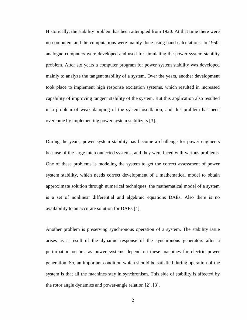
Historically, the stability problem has been attempted from 1920. At that time there were
no computers and the computations were mainly done using hand calculations. In 1950,
analogue computers were developed and used for simulating the power system stability
problem. After six years a computer program for power system stability was developed
mainly to analyze the tangent stability of a system. Over the years, another development
took place to implement high response excitation systems, which resulted in increased
capability of improving tangent stability of the system. But this application also resulted
in a problem of weak damping of the system oscillation, and this problem has been
overcome by implementing power system stabilizers [3].
During the years, power system stability has become a challenge for power engineers
because of the large interconnected systems, and they were faced with various problems.
One of these problems is modeling the system to get the correct assessment of power
system stability, which needs correct development of a mathematical model to obtain
approximate solution through numerical techniques; the mathematical model of a system
is a set of nonlinear differential and algebraic equations DAEs. Also there is no
availability to an accurate solution for DAEs [4].
Another problem is preserving synchronous operation of a system. The stability issue
arises as a result of the dynamic response of the synchronous generators after a
perturbation occurs, as power systems depend on these machines for electric power
generation. So, an important condition which should be satisfied during operation of the
system is that all the machines stay in synchronism. This side of stability is affected by
the rotor angle dynamics and power-angle relation [2], [3].

3
The developments that occur in modern power systems lead to an increasing tendency to
focus on effects of instability, which give the necessity of evolving new techniques to
improve transient stability since it plays a significant role in preserving safety of power
system operation. Power system transient phenomena play an important role in
designing, developing and operating power systems. Investigating this phenomena gives
important information on the machines in showing the ability to maintain their
synchronism throughout wide unexpected perturbation such as various faults, losing
main part of the load and power generation units [3], [5].
Plenty of studies have been devoted over the years to handle the problem of dynamic
stability in power systems. Dynamic simulation should be used to analyze and solve the
stability problem of the power system efficiently. In other words, stability simulation
criteria depend on dynamic model derived [5], [6]. Transient stability simulation problem
is sorted as step by step solution of differential-algebraic initial value problems. This
solution allows reducing the interface error to a more acceptable level [7].
In the present time, power systems are being adjacent to their stability limits because of
the environmental and economic restrictions. Maintaining a stable operation of a power
system is consequently a very important issue and much concentration on the study of
stability problems has been carried out [8]. Analysis methods that take dynamics of the
components in the power system into account like small signal analysis, can efficiently
enhance dynamic performance and augment power transmission of the system [4].

4
Small signal stability (or small-disturbance stability) is the ability of restoring the
operation mode to its original mode or a new mode and maintain synchronism after a
small disturbance. The problem is usually one of the insufficient damping of the system
oscillations, which is caused by the lack of sufficient damping torque. Oscillations will
appear between two or more generators, as soon as AC generators were operated in
parallel [2], [9]. Small signal stability problems could be either local or global mode in
nature. The first mode is related to the oscillations of generating units at a specific station
in regard to the remainder of system. The second mode is related to the oscillations of
many machines in one portion of the system versus machines in the other portions; these
oscillations are named 'inter-area mode oscillation' as well. To analyze and design power
systems, small signal stability is the most significant prerequisite, which consists of
oscillation mode and mode form, correlativity analysis, stability area estimation and its
sensitivity. Small signal stability has many approaches of analysis methods like eigen-
structure analysis which is based on theoretical solution and time domain simulation
based on numerical solution [10], [11].
There are various theoretical and numerical techniques used in power system stability
studies. One of the theoretical techniques is based on Lyapunov’s stability theorem,
which gives a basis for optimal dynamic stability design of power systems. It is applied
to analyze and improve the stability of mathematical solutions of a dynamical system.
One of the studies that have been carried out in [12] is applied by using Lyapunov’s
direct method to get suitable and feasible investigation of the stability of systems with
deviating argument of delay type. The ways of constructing Lyapunov functions for
linear systems with fixed coefficients are already well-established. Although this

5
technique gives satisfactory results, it is not efficient for large power systems and it will
be complicated and difficult to handle for stability problems. Numerical methods are
widely used since they can handle different types of dynamic models and sequences of
events for complex power systems. In other words, they are applicable to analyze several
forms of complex nonlinear phenomena [12], [13].
An interesting case is tracking the system trajectory and determining the tasks needed to
recover and restore the system when imbalance is observed in load-generation. This
needs to integrate the DAEs. For this reason, some techniques are developed and carried
out step by step, integrating the DAEs of the system from the initial value to get dynamic
response to perturbations. The importance of a dynamical simulation tool in power
system transient analysis leads to the use of various kinds of numerical integration
techniques like trapezoidal and Euler methods [6], [14].
The Trapezoidal method of variable step size integration is very efficient, and widely
used. It is one of the good approaches in numerical integration techniques that is used to
insert synthetic elements in the system which could impact the correct solution to a
certain degree. Trapezoidal method is used in [14] to give an efficient solution for a
boundary value problem by immediate calculation of a trajectory on the stability
boundary that is designated as a critical trajectory. Therefore, in this study, the method
depends basically on the calculation of the trajectory for assessment of stability [3], [6],
[14].

6
The Euler method is used in [15] to support C/C++ software to solve the mathematical
representation of power system dynamic equipment which includes synchronous
generators, turbine-governors and exciters. This software is the Dynamic Computation
for Power Systems (DCPS) software package, and it is applied to show the basic
modeling and calculation ways that deal with power system dynamics and carry out
power system transient stability analysis. WECC 9-bus system was used to check the
impact of changing load demand on the critical clearing time Tcc. The outcome showed
that an increase in the load demand leads to linearly decreasing Tcc. The transient
stability is performed to check the response of the equipment for the three-phase fault
case. During this case, critical fault clearing time Tfc is solved, and the system becomes
unstable if Tfc becomes greater than Tcc [15].
Although this approach gives noticeable improvement in the stability solution, it suffers
from some disadvantages that reduce its applicability, such as the lower accuracy and the
synthetic numerical oscillations that are frequently encountered in switching events, and
thus in discontinuities. Furthermore, this method by itself will fail at large step size
integration and it will go to divergence. Another problem is the large number of DAEs in
the mathematical model of a large power system. Therefore, the solution through those
methods needs to be supported and developed by another technique [16].
Recursive projection method (RPM) is stabilization of an unstable numerical procedure;
it is performed by calculating a projection onto the unstable subspace. RPM is applied to
recognize and solve the unstable/slow invariant subspace by obtaining outcome
information from a time domain simulation code TDSC [17]. Newton or special Newton
7
iteration is carried out to improve convergence of the unstable/slowly-converging mode;
in contrast, fixed-point iteration method of the TDSC is utilized and kept to evolve as the
stable/fast-decaying mode of a system. During the numerical process, the projection is
updated effectively, and resizing the dimension of the unstable subspace can be done;
decrease or increase in the dimension can occur. It is notable that this method is quite
efficient in the case of a small size of the unstable subspace compared to the size of full
state system. Furthermore, RPM is effectively applicable to accelerate iterative actions in
case of slow convergence caused by some tardily decaying modes [18].
RPM, which is originally proposed in [18], started to be applied recently in power system
stability problems; it is receiving more attention because of its ability to enhance
convergence and produce eigenvalues as a byproduct from TDSC. Besides that, it
efficiently works by preserving numerical and modeling facilities of TDSCs, and saves in
cost by cancelling additional programming costs [17].
To summarize, a major problem in the numerical stability analysis of power systems is
the inadequacy of the existing time domain numerical simulation methods in predicting
the dynamics of the system after a disturbance. The aim of this thesis is to apply the
RPM procedure to stabilize the numerical simulation of the dynamics of system when a
fault occurs, thus enabling an accurate prediction of system behavior in transients.
This thesis is organized as follows. In Chapter 1 the stability problems in power systems
is surveyed and discussed. Chapter 2 deals with the mathematical formulation of the
stability problem for single-and multi-machines systems, while Chapter 3 introduces the
RPM method and its application to the numerical simulation of power system transients.

8
In Chapter 4, simulation results for a number of test cases are presented and discussed.
Finally, in Chapter 5 some conclusions are drawn and suggestions for future work are
made.

9
Chapter 2
STABILITY ANALYSIS OF POWER SYSTEM
2.1 Synchronous Machines
The main part in an electrical power system that deals with stability analysis is generator
and its rotor part, since it plays a major role in system synchronism. Therefore,
performing dynamic model and developing mathematical equations should be achieved
to describe the dynamics of the rotor and its angle position.
The important thing is when the power system operates in the steady state mode it is
subject to a perturbation. This leads to alteration in the voltage angles of the synchronous
generators. This will produce an unbalance between the generation and load of the
system and will create a new operating mode with different voltage angles.
The stability analysis determines the effect of disturbances on the behavior of
synchronous machines in power systems. The perturbation may be small like changing in
load demand; or large such as loss of generator, line, or a series of such disturbances. The
modification that occurs from the initial (steady state) operating mode to the new
operating mode is called the transient duration, and the behavior of the system during this
time is called dynamic system performance. The main point in stability criteria is
whether synchronous generators preserve their synchronism at the termination point of

10
transient duration. If the oscillatory response of a power system over the transient
duration is damped and the settling of the system occurs successfully to the new steady
operating mode in a limited time, the system will be stable, and if not the system will be
unstable [19].
The system contains inherent forces that tend to reduce oscillations when the system has
ingrained forces, and these forces try to reduce the oscillations, this case known as
asymptotic stability. This type of stability is targeted in the future of power system. The
continuous oscillation is excluded from asymptotic stability, although this type of steady
state oscillation may be considered stable in mathematical analysis. The concern is on the
practical side, because this continuous oscillation may be undesirable to both of the
feeding system and the costumer in electrical power system. The asymptotic stability also
shows the workable characteristic for an agreeable operating state [3], [19].
The stability problem focuses on the behavior of synchronous machines after being
subjected to a disturbance. Therefore, it is important to study the stability analysis of
these machines by performing dynamic modeling and developing mathematical
equations [20].
2.2 Swing Equation
A swing equation is significant in power system analysis for studying transient dynamic
criteria and power oscillations in power systems. At steady-state operating mode, the
relative location of the rotor axis and magnetic field axis is preserved, and the angle
between those two axes is called power (or torque) angle. Over the perturbation period,
the machine rotor will accelerate or decelerate according to the axis of rotation and (or

11
rotating air gap) synchronously and the starting point of rotor motion proportionally. This
motion can be represented by a mathematical equation which is called the swing equation
[2], [19]. After this period, if the machine rotor tends to its synchronous speed, the
generator will preserve its stability. If the perturbation does not produce any change in
power, the rotor will go to its original location. If the perturbation produces a change in
generation or load, the rotor will move to a new operating angle according to the
proportional synchronously regenerating field.
In transient stability analysis, every generator will be represented by two state equations.
After fault clearing, which could include separating fault line, the bus admittance matrix
of the system will be recalculated to reflect the alteration in the system, as well as
recalculating electrical power of ith generator [21]. The new bus admittance matrix could
be reduced because of separating the faulted line. At post-fault case, performing the
simulation will continue to define the stability of the system, and the output plotting will
shows the direction of the system behavior to stable or unstable mode. Generally, the
output solution will be for two swings to approve that there is existence or not of
difference between two swings. If the angle between these two swings is fixed, the
system is stable, if not the system is unstable [22].
At steady state operating mode, all the machines of the system rotate at a similar angular
velocity, but when a perturbation occurs, one or some of the machines may accelerate or
decelerate its angular velocity, this representing a risk on the power system that may
cause loss of synchronism. This problem has affects system stability, and those machines

12
that lose synchronism should be separated from the system. Otherwise, large damage
may occur [23].
2.3 Swing Equation of Single Machine
Consider a system consists of a three phase synchronous generator with its prime mover,
and this generator connected to an infinite bus. Machine model is shown in Figure (2.1)
are the base of swing equation derivation and shows the electro-mechanical oscillations
in power system [19], [24], [25].
Figure 2.1: Power and torque components in synchronous machines
The symbol m refers to mechanical components and the symbol e refers to electrical
components. In synchronous machines, mechanical torque mT and electromagnetic
torque eT are produced, the first one from the prime mover and the second one from the
machine itself. At steady state operation, mT and eT are equal and there is no producing
of acceleration or deceleration torque. That is 0m eT T
At perturbation case, mT will be greater than eT and acceleration torque Ta will appear,
which includes inertia produced from the inertia of the prime mover and the machine as
shown below in Figure (2.1). This torque will cause accelerating of the machine.

13
The mathematical representation of rotor dynamics is described by using Newton’s
second law in the following differential equation [20], [24]
2
2
mm e a
dJ T T T
dt
(2.1)
where
J : Moment of inertia of the machine (kg.m2)
m : Rotor angular site according to a constant axis (rad)
mT : Mechanical torque (N.m)
eT : Electrical torque (N.m)
aT : Net acceleration torque (N.m)
Multiplying both sides by angular velocity m
2
2
mm m e
dJ P P
dt
(2.2)
m m mP T and e e eP T are the effective mechanical and electrical powers on the rotor
m : Rotor angular speed (rad/s)
The formula (2.2) represents the angular acceleration expressed by mechanical angle,
using electrical angle (2.2) becomes,
2
2
2 em m e
dJ P P
p dt
(2.3)
By rearranging the left hand side the resultant equation will be
22
2
2 12 ( )
2
em m e
m
dJ P P
p dt
(2.4)

14
The relationship between mechanical and electrical angular velocity ,m e respectively
of the rotor is
2
em p
(2.5)
Dividing equation (2.4) by the rating of the machine ( S ), and using equation (2.5) give
22
2
1( )
2 2m
e m e
e
Jd P P
S dt S
(2.6)
The electrical quantities are computed by per unit base, as well as moment of inertia J ,
and inertia constant H of the synchronous machine, given by
2
00.5 mJH
S
(2.7)
The practical side of power systems shows that through perturbation, there is no considerable
swerve of angular velocity from the nominal quantities 0 0,m e . After substituting equation
(2.7) in equation (2.6) the resulting form of the equation will be
2
2
0
2 pu puem e
e
dHP P
dt
(2.8)
The symbol pu refers to the mechanical and electrical power values are in . .pu of the
rating of machine. It is acceptable to choose the powers quantities in . .pu at the same
base of synchronous machine. Therefore, the final equation could be written as:
2
2
0
2m e
H dP P
dt
(2.9)

15
2.4 Power - Angle Relation
Assume a simple model of one synchronous generator connected to an infinite bus as
shown in Figure (2.2). To simplify this model, classical model can be taken by
substituting the generator with a fixed voltage behind a transient reactance. In such a
system, there is a maximum power which could be transferred from the generator to the
infinite bus. The relation between the generated electrical power and the rotor angle of
the machine is shown by the following equation [20], [24], [25].
1 2maxsin sine
T
E EP P
X
(2.10)
where
c 1 2max
T
E EP
X
(2.11)
2.5 Equal-Area Criterion
Equal-area criterion is one of the graphical techniques developed to analyze system
stability; the graph shown in Figure (2.3) explains the stored energy in the rotating body
that confirms whether the machine can preserve stability after perturbation. This
technique could be utilized after sharp disturbance occurred to the machine to predict the
stability at a short time (speedily). It is useful for a system consisting one machine
connected to an infinite bus or a two-machine system, but unacceptable for large
systems. For a simple system consisting of one synchronous machine connected to an
infinite bus, it can be presented by a classical model as shown in Figure (2.2)

16
Figure 2.2: Single machine infinite bus system
From (2.9), the following formula can be obtained
0
2
0a
dP d
dt H
(2.12)
while d
dt
is the relative speed according to the rotating base frame, its initial value is
zero. After a perturbation, the machine accelerates and the value of Pa will be positive.
With regard to stability, Pa should reverse its sign after d
dt
reaches to zero. Therefore,
Pa is a function of θ and has a various Pa( ) 0.
0
0aP d
(2.13)
and the limit of Pa
max( ) 0aP and
max
0
0aP d
(2.14)
If the plot of Pa is a function of θ, the formula (2.14) can presents the area under the
curve that limited by θ0 and θmax. The total area under the curve should be zero (the
positive part equal the negative part); based on this it is called as the equal area criterion
[20]. Using (2.11) and fixing Pm
1 2 sine
E EP
X (2.15)

17
while X relies on the status of the system which may be pre-fault, fault or post-fault. The
behavior of the system and the power angle corresponding to those three cases are shown
in Figure (2.3). By using (2.14), it is clear seen that the stability is achieved with fault
clearing angle up to θc, when the two areas A1 and A2 are equal. The system will be
unstable if the fault clearing angle exceeds θc. The maximum value of fault clearing time
that preserves the stability of the system is called critical fault clearing timefcT , and the
corresponding maximum rotor angle is θm. The equal area criterion also has the ability to
calculate the maximum power that can be transferred through the system for a specific
fault script, and to check the system if it is stable or unstable according to the given data
and perturbation [20], [23], [24].
Figure 2.3: Equal area criterion of one machine with infinite bus system

18
2.6 Multi-Machine Power System
Considering a multi-machine system, the equation of the output power of its machine can
be obtained by reducing this system and keeping only the internal machine buses
1
( cos sin )N
ei i k ik ik ik ik
k
P E E G B
1,2,....i N (2.16)
and the swing equations for synchronous machines are
2
2
0
2 i imi ei
H dP P
dt
1,2,....i N (2.17)
By using the trapezoidal method in (2.17)
210
8
n n n
i ei i
i
hP a
H
(2.18)
Where
21 1 1 10
0( ) (2 )8
n n n n
i i i mi ei
i
ha h P P
H
1,2,....i N (2.19)
From (2.16) and (2.19) it is acceptable to solve n
i by applying Newton method, and the
following linear equation is solved for to update .
a J (2.20)
where J is the Jacobian matrix
Power system is a type of big complex systems including generating plants, transmission
grids and distribution substations. To deal with such a system, efficient representation
should be adopted to study the behavior of the system and stability should be analyzed as
well. This can be achieved through mathematical representation by a set of differential
and algebraic equations [20], [24], [25].

19
2.7 Differential Algebraic Equations
In studying the dynamics of a multi-machine power system, different types of stability
problems can be modeled by a set of first-order parameterized differential equations in
the form of
( , , )x f x y p
, : n m p nf R R (2.21)
and algebraic equations in the form of
0 ( , , )g x y p , : n m p mg R R (2.22)
nx X R , my Y R , pp P R
The dynamic state variables x and instantaneous state variables y are distinct in the
state space X Y . The dynamic state variables are time dependent such as generator
voltage and rotor phase, and the instantaneous states variables as bus voltages. The space
P consists of system parameters (as equipment constants e.g. inductance) and operating
parameters (such as generating units and loads). This type of DAEs is used vastly in
numerical solutions and stability estimation in power systems, because it gives realistic
solution for the system's parameters, and it is the easiest utility for sparse matrix
approach as well. Since, it is not general possible to get analytical solution for this
differential algebraic equations (DAEs), approximate numerical techniques are used. The
numerical integration techniques use a stepwise procedure to get a set of solutions for
dependent variables according to a set of solutions for the independent variables.
Integration methods are based on two styles which are explicit or implicit and single-step
or multi-step. Applying integration formula to the solved differential equations separately
is called explicit method, while discretizing those differential equations and solving them
together at the same time as a set is called implicit method. Although the implicit method

20
is too complex it is very useful in numerical stability. Single-step method do not save
previous step values and utilize it in the present step integration, contrary to multi-steps
method which requires storing and using the information of the previous step to solve
the present step integration [26], [27].
In power systems, time domain simulation code (TDSC) is a significant technique for
dynamic analysis. It is used to study the transient behavior by applying numerical
solution to DAEs of such a system. Power system grids consist of many generators,
governors, transformers and various loads. To represent such a grid, each component of
those devices requires differential and algebraic equations; consequently, the total
number of differential and algebraic equations of a power system might be enormously
large. The procedure of time domain simulation of power systems depends on step by
step numerical integration of DAEs. For each corresponding step, there is a numerical
error which can be calculated by local truncation error. To make the solution more
accurate, either small step size integration or high order approximation should be used
[16].
The numerical integration techniques have two classes; explicit and implicit methods.
The explicit method depends on fixed-point iteration with active computation, but it has
numerical stability problems in some cases. The implicit method based on solving
nonlinear equations at each step is more accurately and stable but it is slow. The implicit
method is commonly utilized in power system dynamic simulation, and wide range of
work has been varied out to improve computational efficiency [27].

21
The complexity of the mathematical model will increase for larger scale power systems.
It leads to decreased accuracy of the solution and numerical stability as well.
Consequently, efficient methods should be used to treat these problems and solve DAEs
for various types and scales of power systems such as Modified Euler method,
Trapezoidal method and Runga-Kutta method.
2.8 Modified Euler’s method
The main part of transient stability study is load flow calculation to get system conditions
before a fault occurs. In power systems, it is important to solve first order differential
equations (two for every machine) to get the alterations of both voltage angle and
machine speed. For m machines, there are 2m simultaneous differential equations as
shown in the following equations [28].
( ) 2i t
df
dt
(2.23)
( )( )( )i
mi ei t
i
d fP P
dt H
(2.24)
where, 1,2,........,i m
By assuming the action of the governor is negligible, miP stay constant with(0)mi miP P .
In applications of Modified Euler’s method, the initial appreciations of the voltage angle
and machine speed is obtained at time ( )t t from the following formula
'(0)
( ) ( )
( )
ii t t i i
t
dt
dt
(2.25)
'(0)
( ) ( )
( )
ii t t i i
t
dt
dt
(2.26)

22
Evaluating the derivatives from (2.23) and (2.24) with calculating ( )ei tP allow calculating
powers at time t. While (0)eiP is calculated at the moment just after occurrence the
disturbance.
To obtain the second values, the derivatives at time ( )t t should be evaluated. This step
demand determines the initial values for the machine powers at time ( )t t . Getting
these values of power are obtained by calculating the new components of the internal
voltage according to the following formula
'(0) ' (0)
( ) ( )cosi t t i i t te E (2.27)
'(0) ' (0)
( ) ( )sini t t i i t tf E (2.28)
To get the solution of the network, the voltage at the internal machine buses should be
fixed. By fixing the voltage at the internal machines buses, the solution of the network
can be determined. At fault cases like a three phase fault on the bus ,n the voltage nE is
fixed to be zero. The terminal currents of the machine are calculated by calculating both
of bus and internal voltage as shown in the form
(0) '(0) (0)
( ) ( ) ( )
1( ).
'ti t t ti t t ti t t
ei di
I E Er jx
(2.29)
for the machine powers
(0) (0) '(0) *
( ) ( ) ( )Re ( )ei t t ti t t ti t tP I E (2.30)
The second values of both voltage angle and machine speed are calculated by

23
( ) ( )(1) (1)
( ) ( )2
t t t
i t t i t
d d
dt dtt
(2.31)
( ) ( )(1) (1)
( ) ( )2
t t t
i t t i t
d d
dt dtt
(2.32)
(0)
( )
( )
2ii t t
t t
df
dt
(2.33)
(0)
( )
( )
( )imi ei t t
t t i
d fP P
dt H
(2.34)
The final values of the voltage for the machine buses at time ( )t t are
'(1) ' (1)
( ) ( )cosi t t i i t te E (2.35)
'(1) ' (1)
( ) ( )sini t t i i t tf E (2.36)
Then the solution of DAEs of the network is performed again to get final system voltages
at time ( )t t . The procedure is repeated till it reaches to the ultimate value maxT defined
in the study of such a network.
Modified Euler’s method plays a big role in the calculations of transient stability of
power systems. It can show the behavior of the machines and the performance of the
system. The solution is evaluated by a series of estimates for internal machine bus
voltage and machine speed at the next time step, and repeating this operation allows
evaluating line currents and swinging impedances for preselected lines [28].
Chapter 3

24
RECURSIVE PROJECTION METHOD RPM
3.1 Definition of RPM
Recursive projection method (RPM) is one of the main new techniques to enhance the
stability criteria in power systems. This method is used to stabilize the iterative
procedures of solving nonlinear systems. At each step of iterative procedure, RPM takes
the output information from time domain simulation code (TDSC) to define the
slow/unstable invariant subspace of the full state-space of the system. The full state-
space consists of two invariant subspaces; fast/stable subspace and slow/unstable
subspace. Fixed-point iteration is applied to solve the first one, while Newton method is
applied to improve the convergence of the second one [17], [29].
Since power system is a complex nonlinear dynamic system and can be modeled by a set
of nonlinear differential and algebraic equations DAEs, RPM is investigated in
predicting power system steady state. By taking ordinary differential equation (ODE) of
the system
( , )x F x u
(3.1)
where Nx R symbolizes to state variables, and Su R symbolizes control parameters.
The derivation of Fixed-point iteration method can be done by defining the initial states
(0)x and control parametersu , that is
( 1) ( )( , )v vx x u (3.2)

25
The behavior of solving the iteration (3.2) depends on the dominant eigenvalues of the
Jacobian matrix x at steady state ( )x u , and those eigenvalues control the convergence
of this iteration by their magnitude (largest magnitude), i.e. whether they lie outside or
inside of the unit disk.
{ 1 }U z , < 0 (3.3)
This can be shown by perturbing the solution around its steady state as
( ) ( )v vx x (3.4)
substituting (3.4) in (3.2) and using the first two terms of the Taylor series expansion
( ) ( 1) ( ) ( ) ( ), , , ,v v v v v
x xx x x u x u x u x x u (3.5)
from which we obtain
( 1) ( ),v v
x x u (3.6)
The scheme is convergent and close to steady state operation mode if all the eigenvalues
have a magnitude less than one (located inside the unit disk), and it diverges if any of
those eigenvalues have magnitudes greater than one (located outside the unit disk). In
addition, the scheme is slowly convergent if any of those eigenvalues has a magnitude
close to the boundary. The first case represents a stable scheme and the system operates
in the steady state mode, but the second and third cases represent unstable and critical
scheme and new technique should be applied to solve such problems. RPM is able to
handle these cases; it can retrieve the convergence of the second case and improve
convergence of the third case [17].
3.2 Basic Procedure of RPM

26
The slow convergent or the divergent schemes is the result of from some eigenvalues
approaching (or leaving) the unit disk. The main idea is finding an eigenspace
corresponding to the unstable scheme, which is achieved effectively by recursive
projection method, utilizing iterates from fixed-point iteration [17], [18], [29].
Consider a system has N eigenvalues, and some of those eigenvalues are located outside
the unit disk:
1 .... k 11 ....k N (3.7)
where k is the number of eigenvalues which lie outside the unit disk.
The Jacobian matrix x of the system, which has range spaceNR , can be written as the
direct sum of two subspaces; P which is unstable/slow invariant subspace of x and has
eigenvalues1{ }k
u , and Q which is the orthogonal complement of P
N N NR P Q PR QR (3.8)
Since the stabilization procedure needs to find the projectors P and ,Q it is important to
find an orthonormal basis for the subspace P . This basis is represented by N k
pZ R , and
satisfies T k k
p p kZ Z I R . The orthogonal projector of NR onto subspace P is T
p pZ Z , and
T T
q q p pZ Z I Z Z is the complement orthogonal projector of NR onto subspace Q . The
state variables of the system Nx R can be written as
T
p pp Z Z x P , ( )T
p pq I Z Z x Q (3.9)
by applying the projectors to (3.2), the fixed-point iterations for p and q can be rewritten
as
( 1) ( ) ( )( , , )v v v T
p pp f p q u Z Z ( ) ( )( , )v vp q u (3.10)

27
( 1) ( ) ( )( , , ) ( )v v v T
p pq g p q u I Z Z ( ) ( )( , )v vp q u (3.11)
According to Lemma 1, the procedure will work with the steady state eigenvalues located
all inside the unit disk U and the Jacobian matrix
qg is
( )T
q p pg I Z Z ( , )x x u ( )T
p pI Z Z (3.12)
and the iteration (3.11) is locally convergent in the proximity of steady state.
By using RPM procedure, the convergence of iteration (3.2) is enhanced by applying the
Newton method on the subspace .P At the same time fixed-point iteration scheme is
maintained on subspace Q . The procedure is performed according to the following steps:
by defining the initial states
(0) (0)( )T
p pp Z Z x u , (0) (0)( ) ( )T
p pq I Z Z x u (3.13)
and updating p and q iteratively gives
( 1) ( ) ( ) 1( )v v v
pp p I f ( ) ( ) ( )( ( , , ) )v v vf p q u p (3.14)
( 1) ( ) ( )( , , )v v vq g p q u (3.15)
The iterations (3.14) and (3.15) continues until achieving the convergence at
( 1) ( 1) ( 1)( ) ( )v v vx u x u p q (3.16)
The Newton method is applied to the unstable/slow modes by solving (3.5a) for the
steady state. That is the following equation is solved
( , , ) ( ) ( , , ) 0p f p q u F p p f p q u (3.17)
Newton’s method for iteratively solving nonlinear equations is applied to (3.11) to get
( 1) ( ) 1 ( ) ( ) ( )( , , )v v v v v
pp p F p p f p q u (3.18)
where the Jacobian matrix is given by

28
( ) ( , , )p p
F fF p I I f p q u
p p
(3.19)
Substitution of (3.19) in (3.18) gives (3.14).
3.3 Computational Properties
To get effective computations, the term ( ) 1( )v
pI f requires one formation instead of
updating at each step. The variables kz R are inserted to represent p P :
T T
p pz Z p Z x , pp Z x ,
px Z z q (3.20)
which corresponds to a change of coordinates. It is noteworthy that the Jacobian matrix
related to the Newton part changes its dimensions through performing the RPM
procedure and decreases N N to k k , and the iteration (3.14) is
( 1) ( ) 1( )v v T
p x pz z I Z Z ( ) ( ) ( )( , , )T v v v
pZ z q u z (3.21)
To obtain (3.21), first (3.18) is multiplied by T
pZ and the substitutions
, ( , , ) ( , )T
p p pp Z z f p q u Z Z p q u are made to give
( 1) ( ) ( ) 1 ( ) ( ) ( )
( ) ( ) 1 ( ) ( ) ( )
( ) 1 ( ) ( ) ( )
( ) ( , , )
( ) ( , , )
( ) ( , , )
v v T v T v v v
p p p p
v T T v T v v v
p p p p p p
v T T v v v
m p x p p
z z Z I f Z Z z q u z
z Z Z Z f Z Z z q u z
z I Z Z Z z q u z
(3.22)
where the last line follows from ( , , ) ( , )T
p p p xf p q u Z Z p q u .
It is not necessary to have the system equations in explicit form. This is because the
required computations can be performed implicitly using the information provided by the
TDSC. As a result, the Jacobian matrix also cannot be found in explicit form. Matrix-
vector products are produced from various methods of approximations [17], [18], [29].

29
One of those approximations is shown below. Since the orthonormal basis for the
subspace P are obtained. That is,
1[ ,..., ] N k
p p pkZ Z Z R (3.23)
and for epsilon value < 0, approximating the thi column of
x pZ can be achieved by
the form
[ ( , ) ( , )]x pi piZ x Z u x u / , 1,2,...,i k (3.24)

30
Chapter 4
SIMULATIONS AND RESULTS
The large increase in power demand and preserving the power system stability issue pose
significant problems. To handle such problems and apply efficient techniques that
enhance system stability at various types of operating modes, numerical simulation
should be used. Numerical simulation provides an interactional environment with
thousands of dependable and precise built-in mathematical functions. These functions
give solutions to a wide domain of mathematical problems comprising matrix algebra,
differential equations, non-linear systems, and other numerous kinds of scientific
computations. In numerical simulations, Matlab software is commonly used which has
been strengthened by the effectual SIMULINK program. SIMULINK is a diagrammatic
program utilized to simulate dynamic systems. Besides, it gives the possibility of
simulating linear and nonlinear systems readily and efficiently [25]. Since the dynamical
modeling of power systems is represented by a set of non-linear differential equations, it
is suitable to use such a program to analyze and study power system stability problems.

31
4.1 Case Study
In this study, the numerical simulation has been done by using power system toolbox
PST of Matlab [21]. PST contains a set of M-files developed to aid in exemplary power
system analysis. It supports the user to perform all power system analysis like power
flow solution and transient stability. The power system network chosen as a case study
which consists of three generators and six buses is shown in Figure (4.1).
Figure 4.1: three generators and six buses power system
Here, bus1 is the slack bus with specific voltage 1 1.06 0V , and all the values of
resistance, reactance, capacitance, and voltage magnitude are in per unit and the power
base is chosen as 100 MVA. The power system installation is defined by two certain
matrices for bus and line that are utilized in the load flow computation. Solving load flow
is important to determine the operating conditions that are used in modeling the dynamic

32
devices. Required data is shown in the following tables which include the data set for
generators, loads, buses, and lines.
Table 1: Line data Table 2: Load data
Table 3: Generators data Table 4: Machines data
MACHINES DATA
Gen. aR '
dX H
No. PU PU Sec.
1 0.00 0.20 20.00
2 0.00 0.15 4.00
3 0.00 0.25 5.00
4.2 Transient Stability Simulation Using ode32 Solver
The first step in the numerical simulation of stability is implementing the power flow
solution by using the lfnewton code. This code is based on the Newton method in order
to execute load flow and calculate the physical values like active and reactive power of
the system. Besides, trstab is used with lfnewton to analyze the system after being
subjected to various types of fault, and calculate the new bus admittance matrix. When a
fault occurs in the system, the protection relays directly indicates the fault and sends a
trip signal to the circuit breaker to separate the faulted part.
LINE DATA
Bus Bus R X ½ B
No. No. PU PU PU
1 4 0.035 0.225 0.0065
1 5 0.025 0.105 0.0045
1 6 0.040 0.215 0.0055
2 4 0.000 0.035 0.0000
3 5 0.000 0.042 0.0000
4 6 0.028 0.125 0.0035
5 6 0.026 0.175 0.0300
LOAD DATA
Bus Load
No. MW Mvar
1 0.00 0.00
2 0.00 0.00
3 0.00 0.00
4 100.00 70.00
5 90.00 30.00
6 160.00 110.00
GENERATORS DATA
Bus Voltage Generation Mvar Limits
No. Mag. MW Min. Max.
1 1.06
2 1.04 150.00 0.00 140.00
3 1.03 100.00 0.00 90.00

33
When the system is exposed to a fault, the simulation is divided into three cases; pre-
fault, during fault, and post-fault. The fault may cause a change in the operation mode
according to the voltage values and machine angles as explained in Chapter 2. The aim of
this numerical simulation is to enhance and preserve the stability of the system through
those three steps.
In this dissertation, a fault of three-phase is applied on the line (5-6) close to bus (6).
Separating this line by disconnecting the circuit breakers of the ends of same line, the
fault will be cleared. To carry out transient stability analysis for a specific clearing time
ct and final simulation timeft , trstab code is ran, which is based on the ode32 solver of
Matlab. The first machine is a reference for the other two machines with respect to speed
and angle. For ct = 0.4 s and ft =5 s the output simulation in Figure (4.2a) shows the
oscillations in the angles of both machines. In this case, for ct 0.4 the oscillation will
continue for a certain time with decreasing amplitude before reaching to the steady state.
This is illustrated by choosing ft =30 s as shown in Figure (4.2b).

34
Figure 4.2a: Phase angle difference for both 2nd
and 3rd
machine atft =5 s
Figure 4.2b: Phase angle difference for both 2nd
and 3rd
machine at =30 s

35
To choose best conditions in this code like decreasing the step size to give a solution
with optimal level of accuracy, it still gives unstable solution with oscillation that was
taken as an indication of error in the calculations as shown in Figure 4.2c.
Figure 4.2c: Phase angle difference at best conditions for both 2nd
and 3rd
machine atft =30s
Here, the steady-state solutions for both the 2nd
and 3rd
machine angles are nearly 2.8o
and 6o
respectively. The solution given by trstab for this case shows that the system will
continue oscillating for a specific time after the fault is cleared. Duration of this time is
not short; it may lead to a sequence of other faults and may cause damage to the system’s
switchgear. Although steady-state is achieved after such a long time, the angles still
contain small continuous oscillations. Therefore, if this simulation result is taken to be
reliable, extra work should be done to force the system to return to the steady-state mode
in shorter time, and achieve steady-state without any continuous oscillation as well. On

36
the other hand, the oscillations in the steady state are actually an indication that this
simulation result is not very reliable. Thus, trstab is not that efficient by itself in all the
situations, and the accuracy should be improved by applying an efficient and active
technique, which is the RPM procedure. Also, trstab is based on the ordinary differential
equation solver ode32, which solves the system for a specified span of time, and RPM
requires the solution at each time step in the code. Therefore, ode32 should be replaced
by another solver, which is the Modified Euler Method (MEM), so that RPM can be
easily applied.
4.3 Application of Modified Euler Method
To understand MEM well, it is better to start with the Euler Method (EM). EM is
characterized as the easiest algorithm in the domain of numerical solution of differential
equations, applicable to first order equations. Although EM gives a solution with least
accuracy, it generates a foundation for comprehending more developed methods.
Consider the following differential equation
( )dx
p tdt
x (4.1)
where ( )p t is a known function. According to EM, the derivative in the differential
equation can be approximated by
0
( ) ( ) ( ) ( )lim ( )t
dx x t t x t x t t x tp t x
dt t t
(4.2)
where t is the step size
by rearranging (4.2)
( ) ( ) ( )x t t x t p t ( )x t t (4.3)
by using the iterative procedure (4.3) will be

37
1( ) ( ) ( ) ( )k k k kx t x t p t x t t (4.4)
where 1k kt t t
Euler method can be sum up for the general form ( , )x f t x
as,
1( ) ( ) . [ , ( )]k k k kx t x t t f t x t (4.5)
EM presumes that variables of the equation are constant during the step size t . So, it is
not applicable in all the situations, and has a deficiency in accuracy at a case of fast
changing of variables. To enhance the method, additional update should be applied to the
right-hand side of the equation. The update uses the average of the solutions for two
contiguous steps as below
1 1( ) ( ) ( )2
k k k k
tx t x t f f
(4.6)
where ( , ( ))k k kf f t x t and 1 1 1( , ( ))k k kf f t x t
Thus, utilize EM to get 1( )kx t that allows executing predictor-error method, and MEM
procedure is a combination of the two steps: Euler predictor and predictor-error. That is
Euler predictor 1 . ( , )k k k ky x h f t x
(4.7)
Predictor-error 1 1 1.[ ( , ) ( , )]2
k k k k k k
hx x f t x f t y
(4.8)
4.4 Finding the Jacobian Matrix
The RPM procedure requires the computation of the Jacobian matrix of the difference
equations (see (3.2)) that result from the application of the particular numerical solution
technique to the continuous-time differential equations (DE). In general, the DE’s are
quite complicated and usually very difficult to obtain explicitly. To see how the Jacobian
matrix of the discretized equations of a power system can be indirectly obtained through

38
application of a numerical procedure, we consider a linear second order system with the
equations
1 2
2 1 1 2 2
x x
x a x a x u
(4.9)
which can be represented as ( ) ( )x t F x t where 1 2[ , ]Tx x x and
2
1 1 2 2
( )x
F xa x a x u
(4.10)
Suppose the numerical solution technique applied to (4.7) results in the discrete-domain
equations
1
1
2
( )( )
( )
k
k k
k
xx x
x
(4.11)
The Jacobian matrix of the function vector is given by
1 1
1 2
2 2
1 2
x
x x
x x
This matrix can be evaluated numerically by using the following procedure:
1
[ ( ) ( )] 1,2x n nv x v x n
(4.12)
where v n are the vectors,
1
1
0v
, 2
0
1v
For the Modified Euler method the function vector is written as

39
1( ) [ ( ) ( ( ))]
2
1ˆ[ ( ) ( )]
2
x x h F x F x hF x
x h F x F x
(4.13)
where
1 2
1 1 2 2
ˆ ( )( )
x hxx x hF x
x h a x a x u
(4.14)
evaluation of (4.10) at the predictor solution
2 2 1 1
1 1 2 2 2 1 1 2 2
(1 )ˆ( )
( ) ( )
ha x ha x huF x
a x hx a x ha x ha x hu u
(4.15)
2 2 1 1
2
1 1 2 1 1 2 2 2 2
(1 )
( ) ( ) (1 )
ha x ha x hu
a ha a x a h a ha x ha u
(4.16)
1 2 2 2 1 1
2
2 1 1 2 2 1 1 2 1 1 2 2 2 2
1( (1 ) )
2( )
1( ( ) ( ) (1 ) )
2
x h x ha x ha x hu
x
x h a x a x u a ha a x a h a ha x ha u
(4.17)
finally, the Jacobian matrix can be obtained as
2
1 2
2
1 1 2 2 1 2
1 11 (1 )
2 2( )
1 1(2 ) 1 (2 )
2 2
x
h a h ha
x
h a ha a h a a h a h
(4.18)
The numerical procedure in (4.10) was applied to the system in (4.7) and the computed
Jacobian matrix was compared with the theoretical result (4.11), with an excellent match.
4.5 Transient Stability Simulation Using modeu Solver
After using MEM (modeu) solver instead of ode32 solver in trstab, running lfnewton
and new trstab (which was called eigv) for a three phase fault at the same position (at
bus 6 between lines 5 and 6) the following results are obtained:

40
Figure 4.3: Phase angle difference for both 2nd
and 3rd
machine with MEM at h = 0.01
The similarity of the outputs in Figures (4.2 a) and (4.3) proves that the new code eigv is
working correctly. In this case study, the system contains six state variables; two for each
machine, which are rotor’s speed and angle. Finding the Jacobian matrix allows
calculating eigenvalues and eigenvectors.
4.6 Transformation Region of Stability
When the differential equations of a continuous-time system are transformed to discrete
form by the numerical integration algorithm, the modes of the system will be
transformed according to this relationship
kh
k e
(4.19)
where h integration step size,
( )k x eigenvalues of the discrete mode (integration) system
( )k xF eigenvalues of the continuous mode (physical) system

41
The transformation results in the conversion of the stability zone from the left half part of
the complex plane for xF to the inner region of the unit disk for x . Therewith, applying
numerical techniques to solve ODEs is imprecise. The effective relation is tightly
associated to the integration scheme. For example, this case study deals with the
Modified Euler Method, and for this method,
( 1) ( ) ( )ˆ ( , )v vx x hF x u (4.20)
( 1) ( ) ( ) ( 1)ˆ[ ( , ) ( , )] / 2v v vx x h F x u F x u (4.21)
( )( , )vx u
2[(1 ) 1] / 2k kh (4.22)
4.7 Performing RPM
After calculating the eigenvalues, it should be checked whether their magnitudes are less-
equal-larger than unity. Then the critical values that cause the unstable behavior of the
numerical algorithm is separated, and the corresponding eigenvectors to create a new
basis is found which consequently improves the numerical stability. The result for the
three-phase fault case is shown in Figure (4.4). The operating condition is the same as
before, that is applying a three phase fault between the lines 5 and 6, ct =0.4 s and ft =5
s. The time integration step h is adjustable, and in this case is chosen as h=0.01. After
running the program the magnitudes of the eigenvalues are determined as,
= [1.0000 1.0000 1.0000 1.0000 0.9999 1.0001] , n =6
As shown in , the number of critical eigenvalues are k =5. According to the RPM
procedure, it will produce a matrix of orthonormal basis poZ corresponding to those
critical eigenvalues. The produced poZ is

42
[
-0.0006 + 0.0000i -0.0038 + 0.0000i -0.0742 - 0.5645i 0.0000 + 0.4350i -0.0001 + 0.6975i
-0.0006 + 0.0000i -0.0038 + 0.0000i -0.0756 - 0.5755i 0.0000 + 0.3880i 0.000
poZ
1 - 0.7159i
-0.0006 + 0.0000i -0.0038 + 0.0000i -0.0758 - 0.5771i -0.0001 - 0.8125i -0.0000 + 0.0316i
0.0972 - 0.0000i 0.2980 - 0.0001i -0.0013 - 0.0099i 0.0000 + 0.0029i -0.0000 + 0.0053i
0.5658 - 0.0000i -0.8014 + 0.0002i 0.0004 + 0.0031i 0.0000 + 0.0006i -0.0000 + 0.0011i
-0.8188 + 0.0000i -0.5185 + 0.0001i 0.0003 + 0.0021i 0.0000 + 0.0007i -0.0000 + 0.0014i]
After calculating the solution at time step ,k the Jacobian matrix, and poZ are substituted
in the main equations of the RPM algorithm to give the corrected solution at time step
1k . This solution improves the convergence of the solution and enhances the ability to
evaluate system stability as shown in Figure (4.4)
Figure 4.4: Phase angle difference for both 2nd
and 3rd
machine by RPM
To prove that RPM works efficiently, can check the steady state solutions in both Figure
(4.2) and Figure (4.4) to show that the values of the two machine angles are almost equal.
In addition, RPM reaches the steady-state mode in a very short time 0.45 s comparing

43
with the previous case at 30 s, without any oscillation. The comparison between classical
method and RPM is shown in Figure (4.5 a-b).
Figure 4.5a: Comparison between classical method and RPM
Figure 4.5 b: Comparison between classical method and RPM, showing initial part

44
We have taken a large simulation end-time to see the achievement of RPM clearly, as
shown in Figure (4.6). The numerical solution given by trstab continues to oscillate in
the steady-state, whereas it is perfectly stable with RPM.
Figure 4.6: Steady-state solution of the system by classical method and RPM
One of the best achievements of RPM is performing the solution and reaching steady-state
mode with a time shorter than that in classical methods; this leads to having reliability and
efficiency in the response of system simulations. For a step size h=0.15, the solution for
classical method will give unstable solution, while RPM will preserve the stable solution as
shown in Figure (4.7). Note that the large simulation time here is for observing the behavior of
stability analysis in power system simulation, not for an actual application in real time. In
practice, the time tcc and the steady-state period depend on many conditions like the size of
fault, and the ability of the switchgear and the grid to handle such a fault and pass it
successfully.

45
Figure 4.7: Comparison between classical method and RPM for h =1.5
4.8 Dynamic Simulation Using Power System Toolbox (PST)
Application of RPM at the beginning of this study was carried out by using the power
system toolbox PST [30]. But it was later abandoned because of the difficulties in using
the transient simulation code s_simu in conjunction with the RPM procedure. PST
allows modeling machines and control systems, and establishes active modeling to state
variables for designing damping controllers. These models are coded as m-files Matlab
functions. One of those m-files is s_simu which has driving functions for transient
stability analysis. The code s_simu needs only input data to prepare a good environment
for analyzing and solving the system dynamical equations. First of all, this code was used
and many operating tests have been done on the 9-bus WECC (or WSCC) power system
[23] to see the behavior of the system; showing when and how the system can regain its

46
steady state mode after subjected to different types of faults. This study is stopped in this
thesis when trying to apply the RPM algorithm with s_simu, because it contains complex
steps and it is difficult to connect RPM to it. Therefore, trstab m-file is used instead of
s_simu and the complete work is implemented successfully.

47
Chapter 5
CONCLUSION
In this study, the power system stability problem is considered, and effective ideas are
introduced for efficient analysis of power system behavior for various types of operating
conditions. It has focused on transient stability under specific disturbances. The main
criterion in power system stability, namely the equal area criterion, is also demonstrated
in this study. Mathematical representation of power systems is performed to obtain
differential and algebraic equations that have been solved numerically. In this work,
MEM solver is used because it gives simple and accurate solution, and it is based on time
stepping that allows application of the RPM algorithm easier than using the ODE solver,
which is based on a time span solution.
An effective numerical technique is presented, which is the RPM algorithm, it is a new
approach used in power systems recently to improve stability analysis. RPM is a
stabilization algorithm that has the ability to expand the convergence domain of fixed
point iteration schemes. In other words, RPM evaluates subspaces for the case of
divergent iterations and correcting those iterations by applying Newton's method,
whereas on the supplement, fixed point iteration is preserved to evolve the convergent
iterations. A test example of a 6-bus power system is considered to show the
achievements of the RPM technique and Modified Euler Method in the Matlab

48
environment. Besides, numerical simulation studies performed on such a system have
shown the success of this technique.
At each time step, the Matlab code calculates the Jacobian matrix and finds its
eigenvalues. After that it compares the magnitudes of those eigenvalues, separating the
larger ones and creating a corresponding ortho-normal basis which helps the code to find
the correct solution and stabilize the numerical system.
The RPM procedure represents a useful algorithm in power system stability analysis that
can handle all the operating situations, stable, slow-decaying and unstable modes,
effectively and with high accuracy. As a result, RPM forces power system simulation to
reach the steady-state mode in a very short time compared with conventional procedures,
and without erroneous oscillations.
Future work that may be suggested is the application of the RPM algorithm to larger
power systems, and for the case of unstable invariant subspaces with large dimensions.
Theoretical work should also be carried out on this method to understand the level of
accuracy improvement.

49
REFERENCES
[1] Han, X., Tian, N., et.al., “Small signal stability analysis on power system considering
load characteristics,” Power and Energy Engineering Conf., 2009, pp.1-4.
[2] Grigsby, L.L., Electric Power Engineering Handbook: Power system dynamic and
Stability. New York: Taylor & Francis, 2006.
[3] Kundur, P., Power System Stability and Control. California: McGraw-Hill, 1993.
[4] Su, Y.C., Cheng, S.J., et.al., “Power system dynamic stability analysis and stability
type discrimination,” International Conf. on Power System Technology, pp.1-6, 2006.
[5] Zhao, X., Zhou, J., et.al., “Dynamic modeling and transient stability simulation of a
synchronized generators in power systems,” International Conf. on Power System
Technology, pp.1-6, 2006.
[6] Wang, K., Crow, M.L., “Numerical simulation of stochastic differential algebraic
equations for power system transient stability with random loads,” IEEE Power and
Energy Society General Meeting, pp.1-8, 2011.
[7] Rudnick, H., Hughes, F.M., et.al., “A discrete model approach to power system
transient performance simulation,” American Control Conf., pp.846-852, 1984.
[8] Chakrabarti, S., “Notes on power system voltage stability”,
http://home.iitk.ac.in/~saikatc/EE632_files/VS_SC.pdf, retrieved on Jun 2011.
[9] Yuanzhang, S., Lixin, W., et.al., “A review on analysis and control of small signal
stability of power systems with large scale integration of wind power,” International
Conf. on Power System, pp.1-6, 2010.

50
[10] Gang, W., Hua, Y., et.al., “Power system small signal stability analysis based on
character identification of time domain simulation,” International Conf. on
Advanced Power System Automation and Protection, pp.1444-1448, 2011.
[11] Han, X., Tian, N., et.al., “Small signal stability analysis on power system
considering load characteristics,” Power and Energy Engineering Conf., pp.1-4, 2009.
[12] Pai, M.A., Sauer, P.W., “Stability analysis of power systems by lyapunov’s direct
method,” IEEE Control System Magazine, pp.23-27, 1989.
[13] Davy, R.J., Hiskens, I.A., “Lyapunov functions for multimachine power systems
with dynamic loads,” IEEE Trans. on Circuits and Systems-I: Fundamental Theory
and Applications, vol.44, No.9, pp.796-812, 1997.
[14] Lopes, B.I.L., de Souza, A.C.Z., “Handling voltage studies under a dynamic system
model,” IEEE Power Tech, Russia, pp.1-6, 2005.
[15] Hashim, N., Sallehhudin, A.A., et.al., “Modeling of power system dynamic devices
incorporated in dynamic computation for power systems(DCPS) for transient
stability analysis,” International Electric Machines & Drivers Conf. (IEMDC),
pp.647-652, 2011.
[16] Meliopoulos, A.P., Stefopoulos, G.K., et.al., “Improved numerical integration
method for power/power electronic system based on three-point collection,” IEEE
Conf. on Decision and Control, and European Control Conf., pp.6780-6787, 2005.
[17] Fan, M.H., Ajjarapu, V., et.al., “RPM-based approach to extract power system
steady state and small signal stability information from the time-domain
simulation,” IEEE Trans. on Power Syst., 26, (1), pp. 261–269, 2011.
[18] Shroff, G.M., Keller, H.B., “Stabilization of unstable procedure: the recursive
projection method,” SIAM J. Numer. Anal., vol.30, no. 4, pp.1099-1120, Aug. 1993.

51
[19] Panda, P.C., “Power system stability using Matlab”, http://ethesis.nitrkl.ac.in/277/,
retrieved on July 2012.
[20] Pal, M.K., “Lecture notes on power system stability”,
http://www.mkpalconsulting.com/files/stabilitybook.pdf, retrieved in May2012.
[21] Saadat, H., Power system analysis. New York: McGraw-Hill, 1999.
[22] Andersson, G., “Modeling and analysis of electric power systems”,
http://www.eeh.ee.ethz.ch/uploads/tx_ethstudies/modelling_hs08_script_02.pdf,
retrieved on August 2012.
[23] Singh, B., Sharma, N.K., et.al., “Enhancement of voltage stability by coordinated
control of multiple FACTS controllers in multi-machine power system
environments,” International Conf. on Sustainable Energy and Intelligent Systems
(SEISCON), pp. 18-25, 2011.
[24] Anderson, P.M., Fouad, A.A., Power system control and stability. Iowa: The Iowa
State Univ. Press, 1977.
[25] Saadat, H., Power system analysis. New York: McGraw-Hill, 1999.
[26] Venkatasubramanian, V., Zaborszky, J., et.al., “A stability theory of differential-
algebraic systems such as the power system,”. IEEE International Symposium,
vol.5, pp. 2517-2520, 1992.
[27] Sanchez-Gasca, J. J., D'Aquila, R., et.al., “Variable time step, implicit integration
for extended term power system dynamic simulation,” IEEE Power Industry
Computer Applications Conf., Salt Lake City, USA, pp.183-189, 1995.
[28] Nimje, A.A., Panigrahi, C.K., “Transient stability analysis using modified Euler’s
iterative technique,” International Conf. on power systems ICPS’90, pp.1-4, 2009.

52
[29] Fan, M.H., Wang, C.S.,et.al., “Power system equilibrium tracing and bifurcation
detection based on the continuation of the recursive projection method,”
Generation, Transmission & Distribution, IET, vol. 6, Issue 3, pp.199-206, 2012.
[30] Chow, J.H., Cheung, K. W., “A toolbox for power system dynamics and control
engineering education and research,” IEEE Trans. Power Syst., vol.7, no.4,
pp.1559–1564, 1992.