Embed Size (px)
Citation preview
Power Scheduling at the Network Layer for wireless sensor networks
Barbara HohltEric BrewerUC Berkeley
NEST RetreatJune 2004
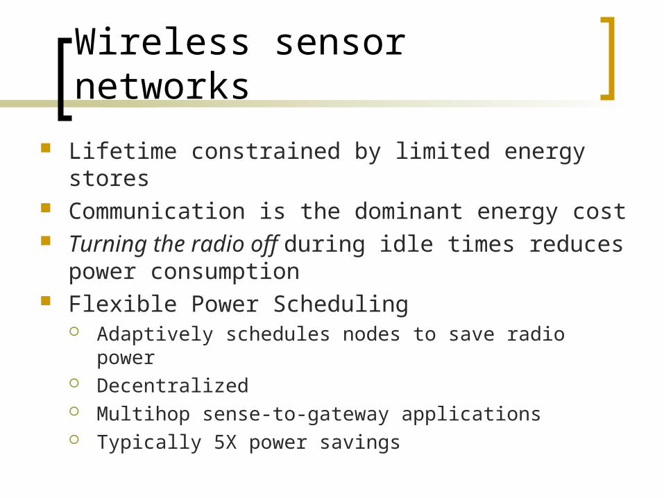
Wireless sensor networks
Lifetime constrained by limited energy stores Communication is the dominant energy cost Turning the radio off during idle times reduces
power consumption Flexible Power Scheduling
Adaptively schedules nodes to save radio power Decentralized Multihop sense-to-gateway applications Typically 5X power savings

Time in seconds
Cur
rent
in
mA
1.4
Overall: 5X Savings

Six Design Principles
Avoid idle listening Use a schedule Two-layer architecture Schedule traffic flows (not packets) Schedules must be adaptive Nodes that want change do the most
listening
Power Schedule
MAC
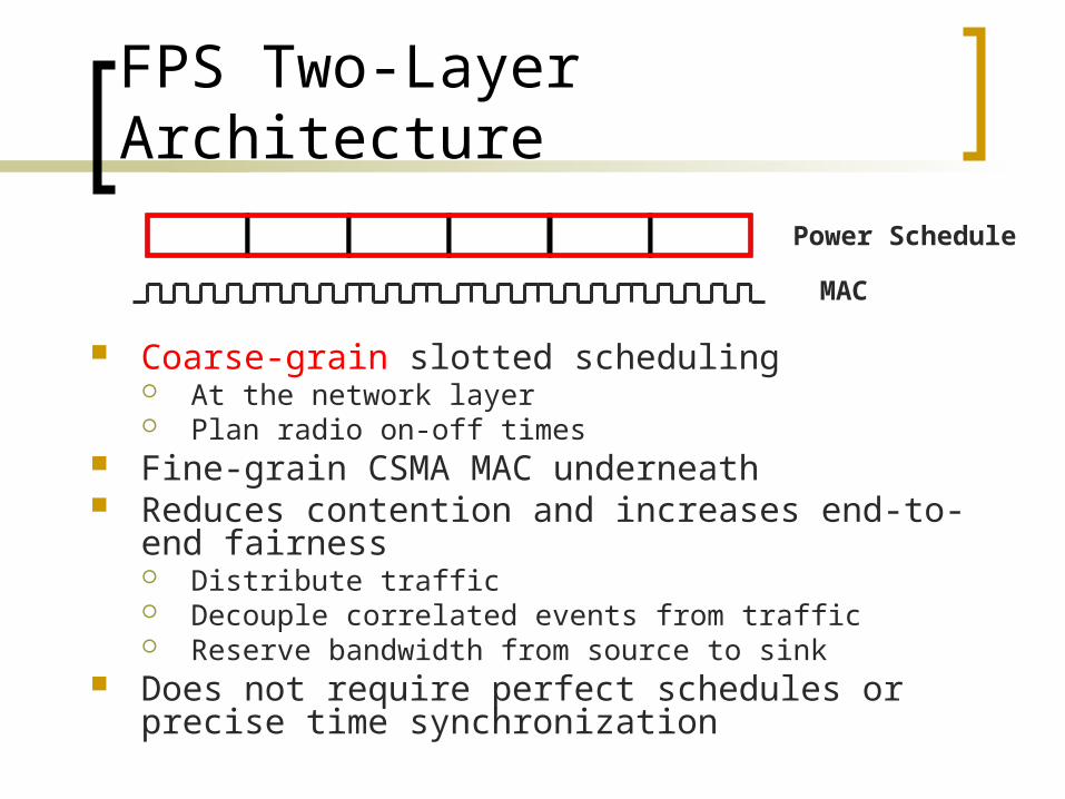
FPS Two-Layer Architecture
Coarse-grain slotted scheduling At the network layer Plan radio on-off times
Fine-grain CSMA MAC underneath Reduces contention and increases end-to-end fairness
Distribute traffic Decouple correlated events from traffic Reserve bandwidth from source to sink
Does not require perfect schedules or precise time synchronization
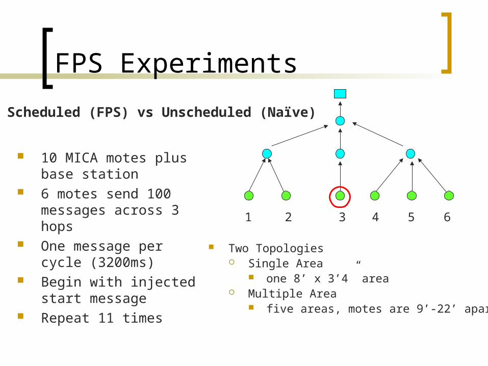
FPS Experiments
10 MICA motes plus base station
6 motes send 100 messages across 3 hops
One message per cycle (3200ms)
Begin with injected start message
Repeat 11 times
1 2 3 4 5 6
Two Topologies Single Area
one 8’ x 3’4” area Multiple Area
five areas, motes are 9’-22’ apart
Scheduled (FPS) vs Unscheduled (Naïve)
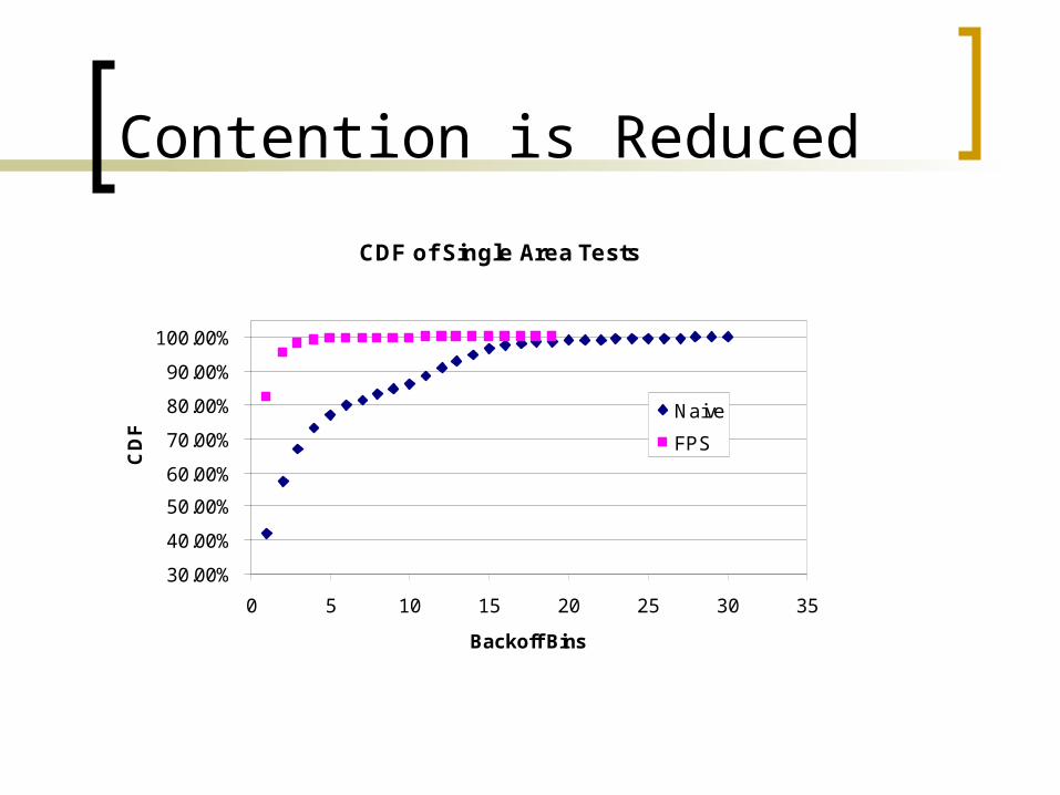
Contention is Reduced
CDF of Single Area Tests
30.00%
40.00%
50.00%
60.00%
70.00%
80.00%
90.00%
100.00%
0 5 10 15 20 25 30 35
Backoff Bins
CD
F
Naive
FPS
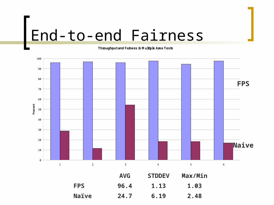
End-to-end FairnessThroughput and Fainess in Multiple Area Tests
0
10
20
30
40
50
60
70
80
90
100
1 2 3 4 5 6
Pe
rce
nt
FPS
Naive
AVG STDDEV Max/Min
FPS 96.4 1.13 1.03
Naïve 24.7 6.19 2.48
Evaluation with TinyDB
Three implementations TinyDB duty cycling TinyDB low power listening TInyDB FPS
Berkeley Botanical Gardens
3 Step Methodology
Estimate radio-on time for each scheme
For FPS, validate the estimate at one mote
Use current measurements to estimate power consumption
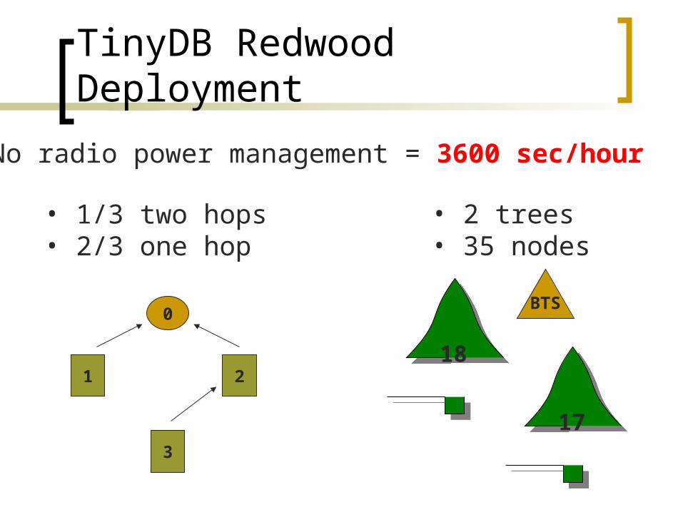
TinyDB Redwood Deployment
17
18
BTS
1 2
3
0
• 2 trees• 35 nodes
• 1/3 two hops• 2/3 one hop
No radio power management = 3600 sec/hour

TinyDB Duty Cycling
4 seconds
2.5 minutes
All nodes wake up together for 4 seconds every 2.5 minutes. During the waking period nodes exchange messages and take sensor readings.
Outside the waking period the processor, radio, and sensors are powered down.
24 samples/hour * 4 sec/sample = 96 sec/hour

Low-Power Listening
Radio-on time = listening + transmitting + receiving
.003 sec/poll * 10 polls/sec * 3600 sec/hour= 108 sec/hour to listen
( 24 samples/hour ) * ( 2/3 * 1 hop + 2/3 * 1 hop ) = 32 hops/hour
32 hops/hour * 0.1 sec/hop = 3.2 sec/hour to transmit
108 (L) + 3.2 (T) + 1.6 (R) = 112.8 sec/hour

Flexible Power Scheduling
18 slots * 128 ms = 2.3 sec/cycle per 3 nodes
= 0.767 sec/cycle (per node)
24 samples/hour * 0.767 sec/cycle = 18.4 sec/hour
0
2
3
1
TrafficComm
Node 1: 2 T, 3 ANode 2: 3 T, 2 R, 3 ANode 3: 2 T, 3 A
5 (node 1) + 8 (node 2) + 5 (node 3) = 18 slots
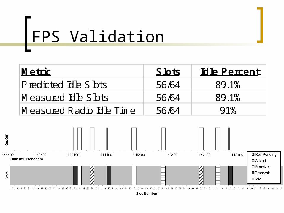
FPS Validation
Metric Slots Idle PercentPredicted Idle Slots 56/64 89.1%Measured Idle Slots 56/64 89.1%Measured Radio Idle Time 56/64 91%

10
100
1000
10000
100000
None DutyCycling
LPL FPS
Cu
rren
t (m
A)
10
100
1000
10000
Sec
on
ds
Off Current
On Current
Total Current
Radio On Time
Power ratios: 160x 4.4x 5.1x 1

Summary
Flexible Power Scheduling Two-level architecture Schedules flows (not packets) Adaptive and decentralized schedules
Reduced contention and increased end-to-end fairness and throughput
Improved power savings of 4.4X over duty cycling and 160X over no power management
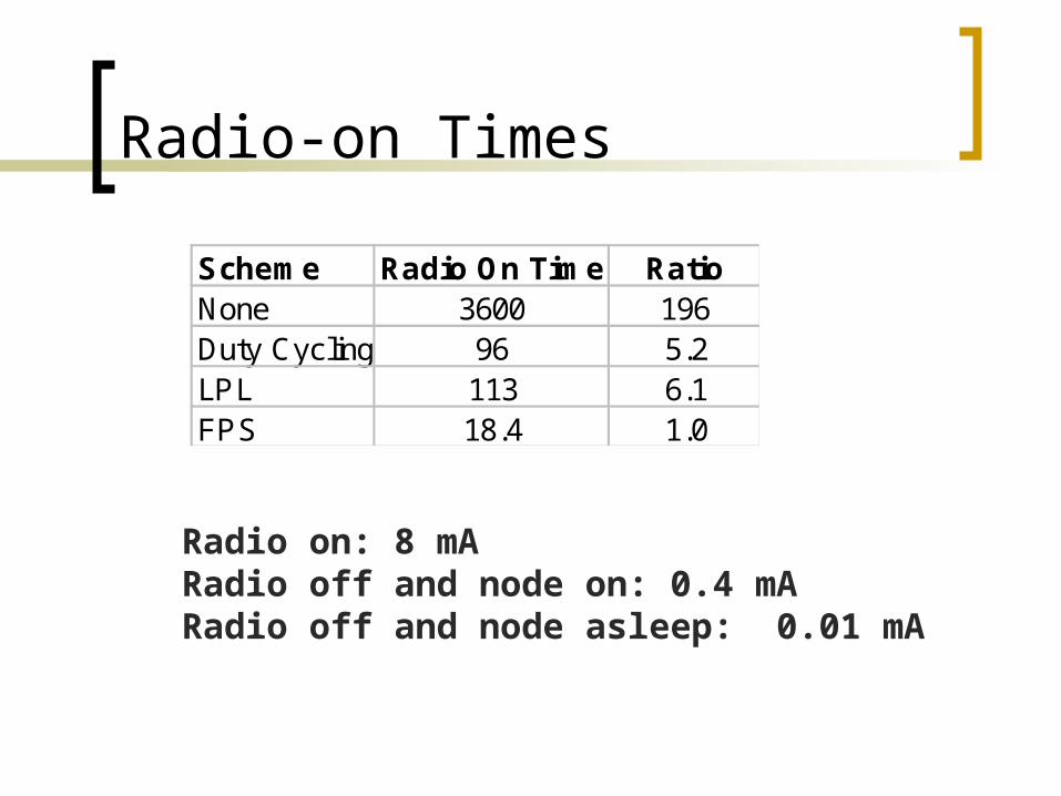
Radio-on Times
Scheme Radio On Time RatioNone 3600 196Duty Cycling 96 5.2LPL 113 6.1FPS 18.4 1.0
Radio on: 8 mARadio off and node on: 0.4 mARadio off and node asleep: 0.01 mA

Power Savings
Scheme Radio On Radio Off On (mA) Off (mA) Total (mA) RatioNone 3600 0 28800 0 28800 157Duty Cycling 96 3504 768 35.04 803 4.39LPL 113 3487 904 34.87 939 5.13FPS 18.4 3582 147 35.816 183.0 1
Scheme Radio On Radio Off On (mA) Off (mA) Total (mA) RatioNone 3600 0 28800 0 28800 18.2Duty Cycling 96 3504 768 1401.6 2170 1.37LPL 113 3487 904 1394.8 2299 1.46FPS 18.4 3582 147 1432.64 1579.8 1
Radio Off and Node Asleep
Radio Off but Node On (Worst Case)

END