Power management in XX systems XX = real-time | …varsha/allpapers/power-aware...Computer Science Department Basics of Energy and Power Power (P) consumption is proportional to the

Computer Science Department

Power management in XX systemsXX = real-time | embedded |

high performance | wireless | …

By:Alexandre FerreiraDaniel Mossé

http://www.cs.pitt.edu/PARTS

Collaborators (faculty):Rami MelhemBruce Childers

PhD students:Hakan AydinDakai ZhuCosmin RusuNevine AbouGhazalehRuibin Xu


Green Computing

Gartner's top strategic technology for 2008: Green IT“This one is taking on a bigger role for many reasons, including an

increased awareness of environmental danger; concern about power bills; regulatory requirements; government procurement rules; and a sense that corporations should embrace social responsibility.”

From Green500.org about supercomputersFor decades now, performance has been synonymous with "speed" (as

measured in FLOPS) emergence of supercomputers that consume egregious amounts of electrical power and produce so much heat that require extravagant cooling facilities

Other performance metrics to be largely ignored, e.g., reliability, availability, and usability.

As a consequence, all of the above has led to an extraordinary increase in the total cost of ownership (TCO) of a supercomputer.


Green Computing

From [Gunaratne et al, IJNM 2005]In the USA, the IT equipment comprising the Internet uses about

US$6 Billion of electricity per year.


Outline and where are we?

Motivation Power consumed by servers, devices, etc Thermal limitations Cost of energy Examples of hw platforms and their E consumptions

Basic techniques Models Hardware Software

HPC + power Products Research projects

Research topics (open problems)


Power Management

Why?Cost! More performance, more energy, more

$$Heat: HPC Servers (multiprocessors), High

performance CPUsDual metrics: maintain QoS, reduce energyBattery operated: satellitesSystem design: Highest component speed

does not imply best system performance


Basics of Energy and Power

Power (P) consumption is proportional to the voltage fed into the component Some systems have a power cap (power limit, cannot operate

above that threshold)

The energy consumed doing a task (E) is the integral in time (T) of the power function. A simple approximation: E = P x T, if P is the average power Some systems have an energy budget (e.g., systems on batteries

or pay-per-use systems with a $ budget)

Thermal dissipation is proportional to the Power (the more power consumed, the more heat is generated) Some systems have a thermal cap More heat generated more cooling needed


Introduction

CPU28%

memory42%

others30%

• CPU (including on-chip caches) and memory energy are major energy consumers

• Energy is a prime resource in computing systems

others51%

memory23%

CPU26%

servers portable devices [IBM] [Celebican’04]

• Power management is subject to performance degradation


Computing Performance

Small Systems – (10s Gigaflops) X86, Power, Itanium, etc.

Specialized CPUs – (1 Teraflops) Cell, GPUs (Nvidia Tesla, ATI)

SMPs – (10s Teraflops) x86, Power, Itanium Shared memory model with up to 1000 cores, 32/64

more common

Cluster – (1 Petaflops) x86, Power, Cell Fastest machines available (Blue Gene and

Roadrunner) up to 128K cores


Power vs Performance Efficiency

Generic CPUsFast but too power inefficient10-100W per core (Athlon 64, Intel Core 2, Power 5/6)New high-performance chips are all multicore

New versions of x86, Power, SPARC.

Power efficient designsCell (100s Gigaflops)

1 embedded PowerPC and 8 SPEs (fast but limited processors)GPUs (1 Teraflops)

Up to 240 dedicated CPUs in a 1.4 B transistors chipCreated for graphics processing, used for parallel applicationsExamples: Nvidia Tesla and AMD Firestream

Floating point accelerators (1 Teraflops)


Power vs Performance Efficiency

Intel ATOM5-6x slower than latest Core 2 processorsBut uses from 0.5 to 2W instead of 30-90W

Whole system design is important Design solved CPU problem: CPU consumes 2W Chipset became the new problem, consuming 20W Bottleneck changed. Will it change again? For sure!


High Performance Computing

Blue Gene/L (~0.3 Gflops/W)Uses a embedded processor design

PowerPC 440 derived design with 2 cores per chipDesign allows 65K CPUs (128K Cores)Fastest machine up to Jun/2008

Roadrunner (~0.4 Gflops/W)Uses a hybrid design

7K Opterons (2 cores) (used for I/O processing)12K Cell processors (FP computation)

Jun/2008: achieved 1 Petaflops


Power in High Performance Computing

Most systems get less than 0.03 Gflops/W

Roadrunner equivalent machine would consume 39MW

Datacenters have an efficiency factor ranging from ¼ (very efficient) to 2 (inefficient) of cooling Watt per computing Watt [HP]

RoadRunner


System Power Management

Objective: Achieve overall energy savings with minimum performance degradation

Previous work in literature target different single component: CPU, caches, MM, or disksAchieve Local energy savings

How about overall system energy?Effects of applying PM in one component on other

system components?Consider the effect of saving power in one component

on the other system components energy.


Memory Power

DDRx DRAMDDR (2.5V), DDR2 (1.8V), DDR3 (1.5V)Bigger memory chips uses less power/bit

Same technologyHigher bus speed increases consumption

Increase bandwidth (faster data transfer)No significant reduction in access time for a single word

(bottleneck in DRAM array) ~1W to 4W per DIMM.

More DIMMs or fewer DIMMs for same size (Total memory)More DIMMs implies parallelism masking some latencyFewer DIMMs reduce memory power


Memory Type # Chips/DIMM Power (W)400MHz/512MB 8 1.30400MHz/1GB 16 2.30400MHz/2GB 16 2.10533MHz/512MB 8 1.44533MHz/1GB 16 2.49533MHz/2GB 16 3.23800MHz/512MB 8 1.30800MHz/1GB 16 1.87800MHz/2GB 16 1.98

02468

1012141618

400M

Hz/512

MB

400M

Hz/1GB

400M

Hz/2GB

533M

Hz/512

MB

533M

Hz/1GB

533M

Hz/2GB

800M

Hz/512

MB

800M

Hz/1GB

800M

Hz/2GB

# Chips/DIMM Power (W)

Kingston Memory

Memory Power Newer technology favors low power designs (lower Vdd)

DDR (2.5V), DDR2 (1.8V) and DDR3 (1.5V) Denser memory is less power hungry (more memory in chip) Higher bus speed implies higher consumption for same

technology


Motivating Example:

CPU and Memory Energy

We can reduce power in processors by reducing speed (using Dynamic voltage scaling DVS)

Memory is in standby for longer periods- energy increases.

en

erg

y

CPU frequency fmaxfmin

Ecpu

Emem

Etot


Other metrics to consider

Maintain QoS while reducing energyQuality of service can be a deadline, a certain level of

throughput, a specified average response timeAchieve the best QoS possible within a certain

Energy budget

Battery operated devices/systems such as satellites. Batteries are exhausted, need to be Replaced (physical replacement is expensive!)Recharged (given constraints, such as solar power)Replace entire device (if battery replacement is not

possible)


Application Characterizations

Different applications will consume different amounts of powerWeather forecastingMedical applications (radiology)Military games (we have no information about it)

One application will have different phases throughout executionUse some units more than others

More memory intensive (e.g., initialization)More CPU intensiveMore cache intensive


High Performance ComputingWeather Prediction

1.5Km scale globally requires 10 PetaflopsNo existing machine can run this modelConventional CPUs (1.8M cores)

US$ 1B to build200MW to operate (US$ 100M per year)

Using embedded processors (20M Cores)US$ 75M to build 4MW to operate (US$ 2M per year)

“Towards Ultra-High Resolution Models of Climate and Weather”, by Michael Wehner, Leonid Oliker and John Shalf, International Journal of High Performance Computing Applications 2008; 22; 149


High Performance ComputingTomography (Image reconstruction)

4 Nvidia 9800 GX2 (2 GPUs per card) in a PC Faster than 256 cores AMD opteron 2.4GHz cluster

(CalcUA) €4000 cost with 1500W consumption University of Antwerp


Application CharacterizationsCan we characterize usage of units within

processor?

How much cache vs DRAM vs CPU vs…Applications have different behaviors

Next slides how these behaviors for

the 3 metrics mentioned: L2 cache, CPU, and DRAM, and for

4 applications from SPEC benchmark: art, gcc, equake, and parser


Workload VariationsCPI: Cycles Per Inst

L2PI: L2 access Per Inst

MPI: memory access Per Inst.














Power Management

Why? Cost! More performance, more energy, more $$ Heating: in HPC Servers (multiprocessors) Dual metrics: maintain QoS, reduce energy Battery operated: satellites System design

How and why?Power off unused parts: disks, (parts of)

memory, (parts of) CPUs, etcGracefully reduce the performance

Voltage and frequency scalingRate scalingTransmit power scaling



Motivation Power consumed by servers, devices, etc Thermal prohibitions Cost of energy Examples of hw platforms and their E consumptions





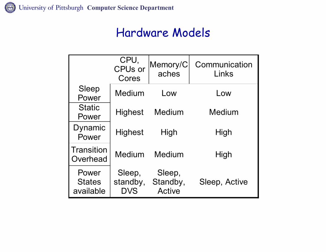
Hardware Models

Medium Low Low

Highest Medium Medium

Highest High High

Medium Medium High

Sleep, Active

CPU, CPUs or Cores

Memory/Caches

Communication Links

Sleep PowerStatic Power

Dynamic Power

Transition Overhead

Power States

available

Sleep, standby,

DVS

Sleep, Standby,

Active


Need to organize the next few slides on the Power Model


Power Models

Dynamic voltage scaling (DVS) is an effective power/energy management technique

Gracefully reduce the performance to save energy CPU: dynamic power

Pd = Cef Vdd2 f

Cef : switch capacitance Vdd : supply voltage f : processor frequency linearly related to Vdd

Frequency( f )

Power( p )

p ∞ f 3


CPU energy model

Power components: Dynamic:Leakage:

Pd=kα CV 2 f

P l=lV−V t

V

spee

d

time

Dynamic Voltage Scaling (DVS): reduce voltage/freq. linearly, reduces energy quadratically


DVS Power and Energy Models

A more accurate power model is:P = Ps + h (Pind + Pd)where:

Ps represents sleep power (consumed when system is in low power mode)

h is 0 when system is sleeping and 1 when activePind represents activity independent power

Memory static power, chipset, communications links, etc.

Pd represents activity dependent powerPd = Cef Vdd

2 f CPU power


DRAM memory energy model

Dynamic and static Power components Dynamic power management

Transition the DRAM chips to lower power stateEx: Rambus {active, standby, nap, powerdn}Energy vs. trans power and delay

P0

P1

P2

Memory requests


Memory Power Model

Memory State

Active:

Standby:

Pa = Total power in active mode

Ps = Static power in active mode

Tac = Measurement time

M = Number of memory access over period Tac

Eac = Energy per memory access

Pa=Ps+ME ac

T ac

Pst


Cache Energy Model

Cacti 3.0 power and time models Access latency and energy are fn. of:

Cache size, associativity and block sizeLonger bit/word lines ==> higher latency



Motivation Power consumed by servers, devices, etc Thermal prohibitions Cost of energy Examples of hw platforms and their E consumptions





Hardware capabilities

Sending power

Link rates (encoding)

Multi-clock domain procs

Real-time

Performance

DVS

TimeoutTimeout

Redundancy (use or add)

Timeout

Redundancy (use or add)

On-off

communication links

memory and/or caches

CPU, CPUs or Cores

Biggest problem is still who manages it, at whatgranularity (physical and power), and how often


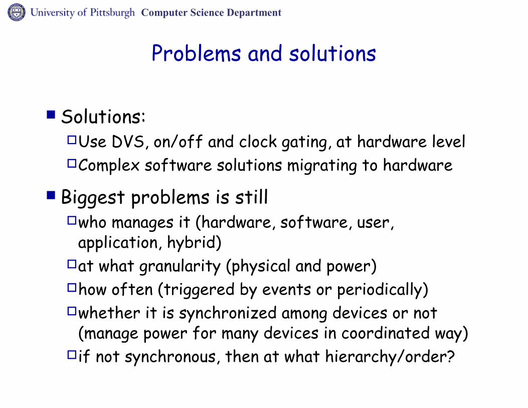
Problems and solutions

Solutions:Use DVS, on/off and clock gating, at hardware levelComplex software solutions migrating to hardware

Biggest problems is stillwho manages it (hardware, software, user,

application, hybrid)at what granularity (physical and power)how often (triggered by events or periodically)whether it is synchronized among devices or not

(manage power for many devices in coordinated way)if not synchronous, then at what hierarchy/order?


Run-timeinformation

Compiler(knows future

better)

OS(knows past

better)

Who should manage power?

Static analysis

Application Source Code

scheduling at the HW level scheduling at the OS level compiler analysis (extracted) application (user/programmer furnished) multi-layer and cross-layer


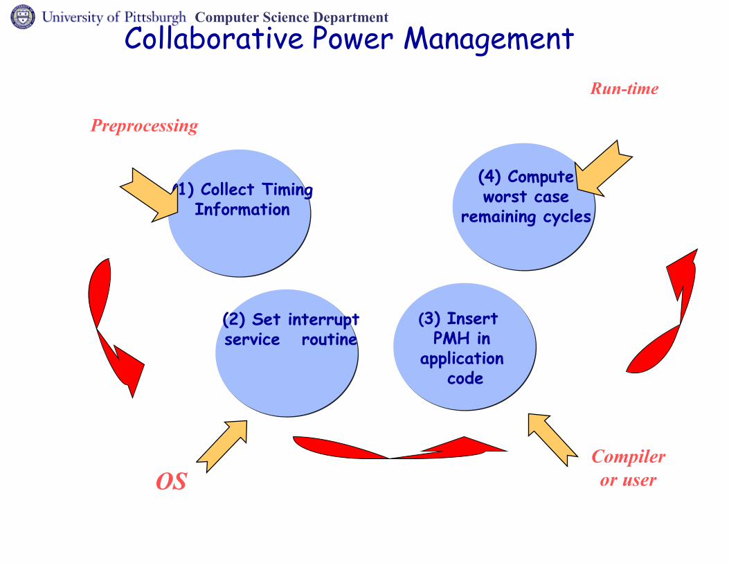
Collaborative Power Management

(1) Collect Timing Information

(4) Compute worst case

remaining cycles

(2) Set interrupt service routine

(3) Insert PMH in application

code

OSCompiler or user

Preprocessing

Run-time


Metrics to optimize• Minimize energy consumption• Maximize system utility• Most importantly, etc!

Time constraints(deadlines or rates)

Energy constraints

System utility(reward)

Increased reward with increased execution

Determine the most rewarding subset of tasks to

execute

Determine appropriate versions to execute

?


Start with hardware solutions

“Doing hardware”, use:Lower power components

Lower frequency of operationP ~ f2 so bigger power gains with smaller performance loss

Clock gatingTurning off circuits whenever they are not needed:

Functional units, cache lines, etc.Used in any large CPU today

ThrottlingReduce utilization by holding requests

DVSChange supply voltage to reduce power


Start with memory (no real reason, should we come up with one that sounds good?? )


Memory energy savings

Low power DRAM system (AMD systems)Uses DDR2-DRAM memory



Uses FB-DRAM memory (Intel Systems)



Different systems will consume different amounts of power in memory Need to characterize bottleneck Deal with memory savings whenever needed!

Timeout mechanisms: Turn memory off when idleTurn some parts of memory off when idle

Power states, depending on how much of the chip is turned offSelf-refresh is the most “famous” or well-known

Who manages timeouts?



Exploiting existing redundancyDistribute workload evenlyOn-off (or in general Distribute workload unevenly)

Adding hardwareCaching near memoryFlash or other non-volatile memoryMore caching at L1, L2, L3

Exploit power states (in increasing order of power)Powerdown (all components are off)Nap (self-refresh)StandbyActive


Near-memory Caching for Improved Energy Consumption


Near-CPU vs. Near-memory caches

Thesis: Need to balance the allocation of the two for better delay and energy.

CPU

Main Memory

cachecache

Caching to mask memory delays

Where? In Main Memory?In CPU?

Which is more power and performance efficient ?

cache


Cached-DRAM (CDRAM)

On-memory SRAM cache [Hsu’93, Koganti’97]

accessing fast SRAM cache Improves performance.

High internal bandwidth use large block sizes

How about energy?

On-memory block size


Near-memory caching:Cached-DRAM (CDRAM)

On-memory SRAM cache Accessing fast SRAM

cache Improves performance.

High internal bandwidth use large block sizes

CDRAM improves performance but consume more energy

On-memory block size


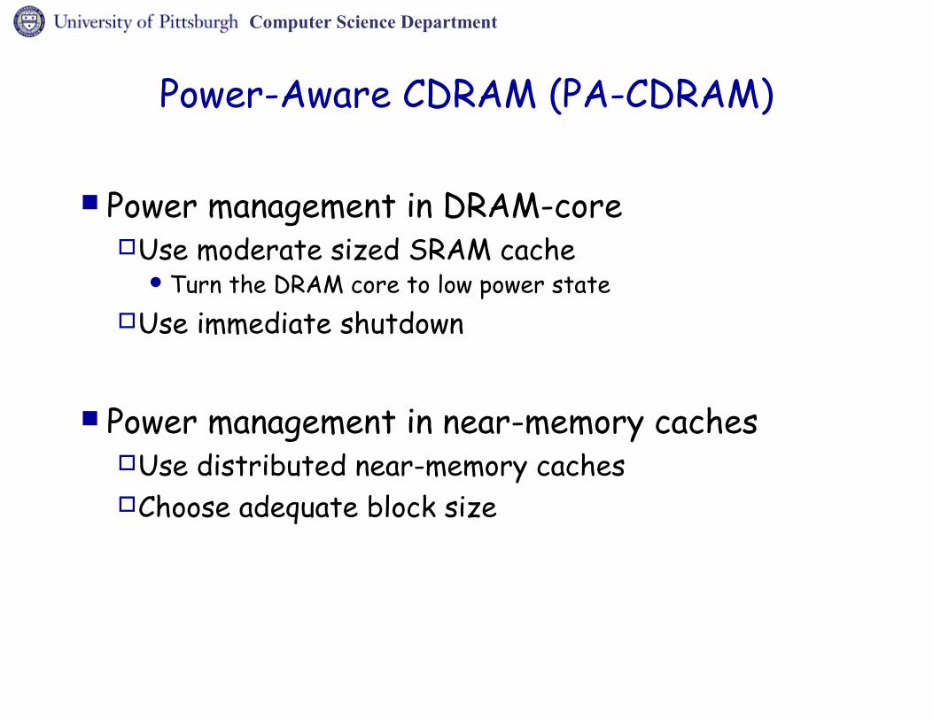
Power-Aware CDRAM (PA-CDRAM)

Power management in DRAM-coreUse moderate sized SRAM cache

Turn the DRAM core to low power stateUse immediate shutdown

Power management in near-memory cachesUse distributed near-memory cachesChoose adequate block size


Power-aware Near-memory Cache vs. DRAM energy

PA-CDRAM energy: Etot = Ecache + EDRAM

0

15

30

45

60

64 128 256 512 1024 2048

block size (byte)

En

erg

y (m

J)

0

0.3

0.6

0.9

1.2

64 128 256 512 1024 2048

block size (byte)

En

erg

y (m

J)

CPU intensive (bzip) memory intensive (mcf)E_DRAME_cache E_tot


PA-CDRAM design


PA-CDRAM new Protocol

Need new commands:To check whether data is in cacheReturn data from cache, if soRead data from DRAM core, if not


Power-aware CDRAM Power management in near-

memory cachesDistributed near-memory

cachesChoose adequate cache

configuration to reduce miss rate & energy per access.

Power management in DRAM-coreUse moderate sized SRAM

cacheTurn the DRAM core to “low

power state”Use immediate shutdown

Near-memory versus DRAM energy tradeoff – cache block size

64 128 256 512 1024 20480

15

30

45

60

block size (byte)

En

erg

y (m

J)

E_DRAME_cache E_tot


Exploiting memory power management

Carla Ellis [ISLPED 2001]: memory states...

Kang Shin [Usenix 2003] and Ellis [ASPLOS 2000]: smart page allocation, turn off pages that are unused.


Integrated CPU+XX DVS


Independent DVS : Basic Idea

DVS sets the frequency of a domain based workload: speed α workload

If workload measured by performance counters# instruction for CPU-coreL2 access for L2-cache # of L2 misses for main

memory Control loop

periodically measure workload to set speed

Domain

Workload

Voltage setting

Voltage controlle

r

Work

load

Volt

ag

e

time

time


Problem: Positive Feedback Intervals

Cach

e f

req

intervals

CPU

w

ork

load

intervals

L2

work

load

intervals

CPU

fre

q

intervals

More stalls Fewer L2 accesses

Slower inst. fetch

higherL2 lat.

More stalls

CP

U D

om

ain

L2 D

om

ain

Freq. of positive feedbac

ks


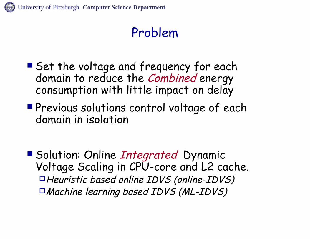
Problem

Set the voltage and frequency for each domain to reduce the Combined energy consumption with little impact on delay

Previous solutions control voltage of each domain in isolation

Solution: Online Integrated Dynamic Voltage Scaling in CPU-core and L2 cache.Heuristic based online IDVS (online-IDVS)Machine learning based IDVS (ML-IDVS)


Integrated DVS (IDVS)

Consider two domain chips CPU and L2 cache

Voltage Controller (VC) sets configuration using observed activity configure using DVS

This also works for different types of domains (e.g., CPU and memory)

VC

L2 Domain

CPU Domain

L1 c

ach

e

FUs

L2 cache

Processor Chip

Main memory


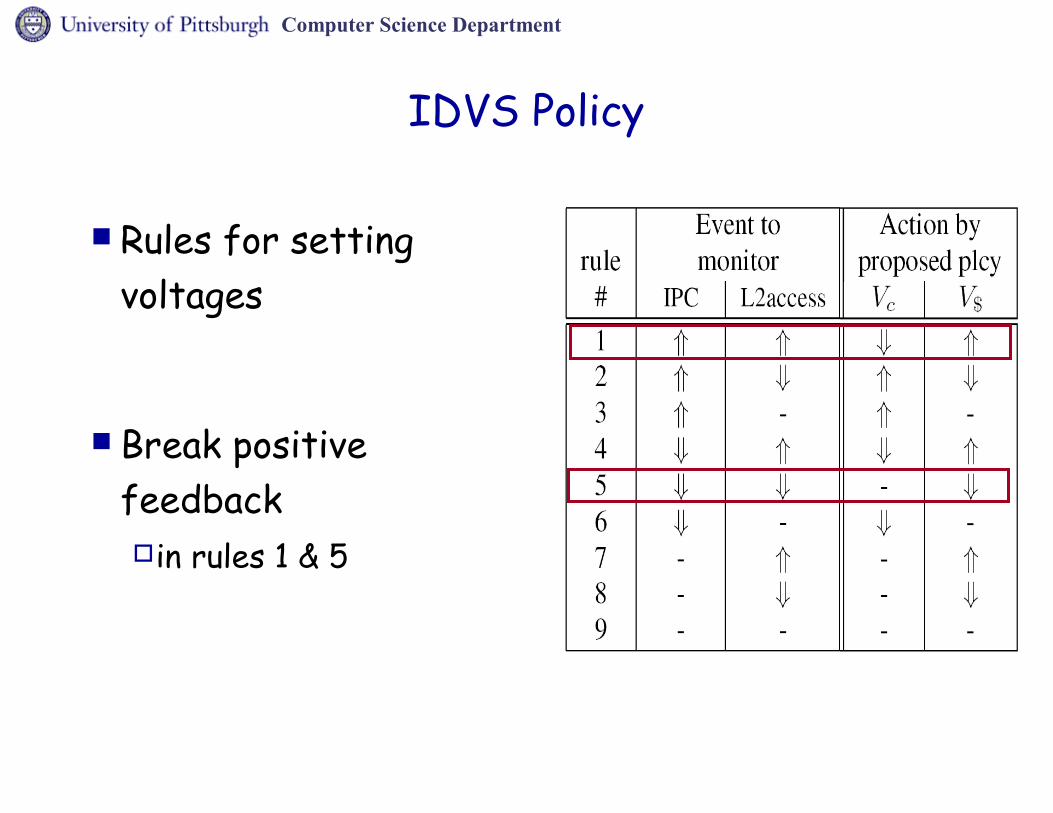
IDVS Policy

Rules for setting voltages

Break positive feedback in rules 1 & 5


Positive Feedback Scenarios

• Workloads increase in both domains (rule 1)– Indicate a start of memory bound program phase

• Preemptively reduce core speed • Increasing core speed will exacerbate load in both domains. • Decrease core speed rather to save core energy

• Workloads decrease in both domains (rule 5)– Longer core stalls are a result of local core activity

• Increasing or decreasing the core speed may not eliminate the source of these stalls.

• Maintain the core speed unchanged

-5

1

V$VcL2 accessIPCRule #


Machine Learning (ML-IDVS): general idea

Training phase

Runtime

Learning engine

determine freq. & voltages

Integrated DVS policy

Auto. policy generator


Learning approach I: Obtain training data

<1, 0.5, 4, 0.05, 0.0002>

<1, 0.5, 2, 0.15, 0.006>Applicationexecution

Applications divided into interval called state State: <operating frequencies, features>

ex: <fcpu, fL2, CPI, L2PI, MPI>


Learning approach

fcpu=1, f$=1

fcpu=1, f$=0.5

fcpu=0.5, f$=1

fcpu=0.5, f$=0.5

<1,1, 4, 0.05,0.001, 5, 0.4>

<1,0.5, 3.5, 0.05, 0.004, 4.2, 0.45>

<0.5,1, 2.5, 0.05, 0.0003, 4.4, 0.55>

<0.5,0.5, 2.4, 0.05, 0.001, 4.5, 0.6>

min E.D

State Table indexed by<fCPU, fL2, CPI, L2PI, MPI>Stores best frequency combinations

< fcpu, fL2, CPI, L2PI, MPI, delay, energy>

If (L2PI >0.32) and (CPI<2) and (MPI > 0.0003) then fL2= 1GHz

else fL2 = 0.5GHz

If (MPI >0.002) and (CPI<3) and (MPI< 0.001) then fcpu = 0.5GHz

else fcpu = 1GHz

Machine learning to generate policy rules

(1) Obtain training data

(2) State-table construction

(3) Generation of rules


Power scheduling


Power-Aware scheduling

Main idea is to slowdown the CPUthus extend the computation

Compute the maximum delay that should be allowed Consider:

Preemptions, high priority tasksOverhead of switching speeds within a task, or when

switching speeds due to task resume

Model dictates as static speed as possible (quadratic relationship of voltage and frequency)


Voltage and frequency relationship

Hidden assumptions:Known execution timesQuadratic relationship of V and fContinuous speeds

Linux has several “governors” that regulate voltage and frequencyOnDemand is the most famous, implemented in

the kernel, based on the CPU utilization.Userspace and Powersave are the other two,

and can be used by applications


Linux OnDemand

For each CPUIf util > threshold --> increase freq to MAXIf util < threshold --> decrease freq by 20%

Parameters: ignore_nice_load, sampling_rate, sampling_rate_min,

sampling_rate_max, up_thresholdDown threshold was 20%, constantNewer algo keeps CPU at 80% util


Power Aware Scheduling for Real-time (cont)

Static Power Management (SPM)Speed adjustment based on remaining execution

time of the taskA task very rarely consumes its estimated worst

case execution time (WCET) Being able to detect whether tasks finish

ahead of (predicted) time is beneficial Knowledge of the application is also good

Knowing characteristics of application and system allows for optimal power and energy savings


Power Aware Scheduling for Real-time

T1

Dfmax

time

Static Power Management (SPM) Static slack: uniformly

slow down all tasks Gets more interesting

for multiprocessors

T2

EStatic Slack

Energy

fT1 T2

idle

timeT1

timeT2

T2

T1

0.6E

0.6E

timeT1 T2

fmax/2 E/4


Basic DVS Schemes

slack

slack

slack

Proportional Scheme

Greedy Scheme

Statistical Scheme


Dynamic Speed adjustment

time

time

WCET

ACET



time

time

Remaining WCET

Remaining time

Speed adjustment based on remaining WCET



time

time

Remaining WCET

Remaining time




time

time



More assumptions

Even for real-time systems, another (huge?) assumption is the knowledge of the execution times of the tasks, which can be obtained throughCompiler-assisted User informedProfiling

Without exact information about the execution times of the tasks, cannot determine a constant optimal speedUse distribution information about the timesWhat distribution, what mean, what average, etc makes a

difference


Schemes with Stochastic Information

The intuition: compute the probability of a task finishing early, and reduce the speed based on that.

Thus, the expected energy consumption is minimized by gradually increasing speed as the task progresses, first named Processor Acceleration to Conserve Energy (PACE) in 2001

1

0

cdf(x)

X


Schemes with Stochastic Information

Existing schemes, such as PACE and GRACE, differ on the way they compute the speed (based on how they define the problem.

Many schemes have the following shortcomings:use well-defined functions to approximate the actual

power functionsolve the continuous version of the problem before

rounding the speeds to the available discrete speedsdo not consider the idle powerassume speed change overhead is zero


Practical PACE

To make PACE practical, algorithms mustUse directly discrete speedsMake no restriction on the form of power functionsTake the idle power into considerationConsider the speed change overhead

Quantize spaces: continuous discrete Cannot look at all combinations of speeds: too

computationally expensiveCarry out optimizations to reduce the complexity


Problem Formulation

Minimize ∑0≤i≤r

si⋅F i⋅e f i

Subject to ∑0≤i≤ r

sif i

≤D

where si=bi+1−b i

F i= ∑b i≤ j<bi+1

1−cdf j−1

1

0

b0=1 b1 b2 b3 br br+1=WC+1

cdf(x)

Xf0 f1 f2 fr…

………


Graphical Representation of the Problem


Graphical Representation of the Problem

The problem is reduced to finding a path from v0 to vr+1 such that the energy of the path is minimized while the time of the path is no greater than the desired completion time D


A Naive Approach

v0 v1 v2 v3

|LABEL(0)|=1 |LABEL(1)|=M |LABEL(2)|=M2

|LABEL(3)|=M3

Exponential growth!


Elimination of Labels

The key idea is to reduce and limit the # of labels in the nodes (after each iteration)

There are two types of eliminationsoptimality preserving eliminationseliminations that may affect optimality but

still allows for performance guarantee


Optimality Preserving Eliminations

• For any label, if the deadline will be missed even if the maximum frequency is used after this point, we eliminate it.

For any two labels, if one is dominated by the other, we eliminate the one which is being dominated If (e,t) ≤ (e’, t’), we eliminate (e’, t’)

�

Eliminate all labels whose energy is greater than an upper bound (e.g., solutions where frequency is rounded up to the closest discrete frequency)


Optimality Preserving Eliminations

v0 v1 v2 v3

|LABEL(0)|=1 |LABEL(1)|=M |LABEL(2)|=M2

|LABEL(3)|=M3

|LABEL(1)|<<M,

Hopefully!

|LABEL(2)|<<M2

Hopefully! |LABEL(3)|<<M3

Hopefully! After the first type of eliminations, the size of LABEL(i) would

decrease substantially. However, the running time of the algorithm still has no polynomial time bound guarantee


Eliminations Affecting Optimality

For a node, we sort the labels on energy and eliminate part of the labels such that the energies of any adjacent remaining labels are off by at most δ

We choose δ carefully: solution is guaranteed to be within a factor of 1+ε of the optimal

PPACE is a so-called Fully Polynomial Time Approximation Scheme (FPTAS) that can obtain ε-optimal solutions, which are within a factor of 1+ε of the optimal solution and run in time polynomial in 1/ε


Stochastic power management

slack

β1D (1-β1)D

D

β1


Computing βi in Reverse Order

β4=100%

β3=xx%

vs.

T1 T2 T3 T4

β2=xx%

vs.

vs.

β1=xx%


An alternate point of view

timeWCE WCE WCE

time

WCET

ACET

time

AV

WCE WCE

WCE

Reclaimed slack

stolen slack


Run-timeinformation

Compiler(knows

future, cansteal)

OS(knows

past, canreclaim)

Return to question:Who should manage?

Static analysis

Application Source Code

PMHs: Power management hints

PMPs: Power management

points

Interrupts for executing PMPsInterrupts for executing PMPs

PMHs PMHs

time


Following slides are on compiler’s ability to insert code, etc


Inter-task vs. Intra-task DVS

deadline

spee

d

time

Intra-task speed changes

# speed changes

Ene

rgy

cons

umpt

ion

Return to question: where to manage

How many and where?


Collaborative CPU power management

OS-directed vs. compiler-directed intra-task DVS.Ex: Gruian’01, Shin et al.’01

Cross-layer scheme uses path-dependant information AND runtime information

Compiler provides hints (PMH) about the application progress to the OS to schedule the speed.

tim

e


Compiler and OS collaboration

Compiler Inserts PMHs in code

to compute timing info.

OS periodically compute and sets new speed

PMHs inserted PMHs inserted by the compilerby the compiler

OS interrupt OS interrupt invoked for invoked for

executing PMPsexecuting PMPs

Interrupt interval

time


OS role

Periodic Execution of ISR

Interrupt interval controls no. of speed changes

ct = read current time

f_curr = read current freq

f_new = calc_Speed(ct,d, WCR)

If (f_new ≠ f_curr)

Lookup power level(f_new)

Set_speed (f_new)

Interval_time = interval_cycles/f_new

rti

# of PMPs

Ene

rgy

cons

umpt

ion


Compiler role

Profiling phase to determine interrupt interval

PMH placement and WCR computationbranches, loops, procedure

bodies,…, etc.

PMH 1

PMH 2

PMH 3

PMH 4 PMH 5

Call P()


CAVEAT: non-linear code

• Remaining WCET is based on the longest path• Remaining average case execution time is based on the branching probabilities (from trace information).

At a

p3p2p1

min average max


Switch gears: mention different possible optimizations


Maximizing system’s utility(as opposed to minimizing energy consumption)

Time constrains(deadlines or rates)

Energy constrains

System utility(reward)

Increased reward with increased execution

Determine the most rewarding subset of tasks to

execute

Determine appropriate versions to execute


• Continuous frequencies, continuous reward functions • Discrete operating frequencies, no reward for partial

execution• Version programming – an alternative to the IRIS (IC)

QoS model

Many problem formulations

Optimal solutions Heuristics

EXAMPLEFor homogeneous power

functions, maximum reward is when power is allocated

equally to all tasks.

Add a task

if constraintsis violated

Repair schedule

yes

no


Satellite systems(additional constraints on energy and power)

time

Available power battery

Use to store (recharge)

splitmerge

consume

Schedulable system

Solar panel (needs light) Tasks are continuously executed Keep the battery level above a threshold at all times Frame based system Can apply three (any) dynamic policies (e.g., greedy, speculative

and proportional)

Example:


MultiCPU systems


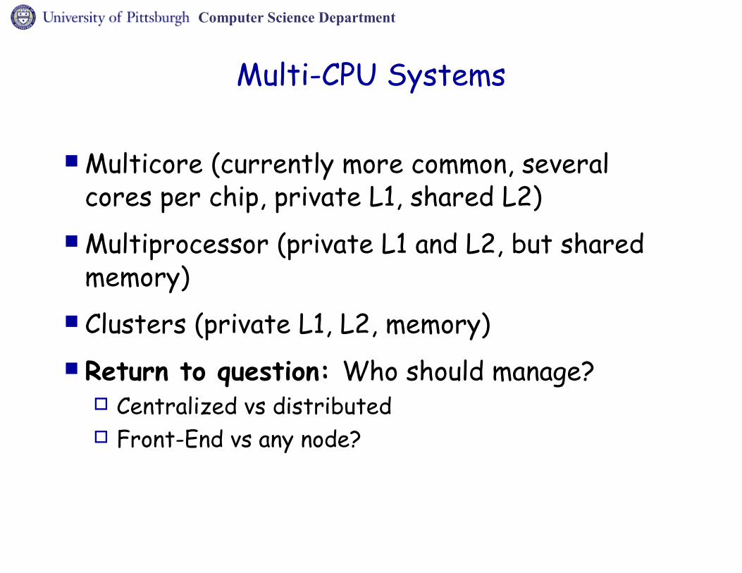
Multi-CPU Systems

Multicore (currently more common, several cores per chip, private L1, shared L2)

Multiprocessor (private L1 and L2, but shared memory)

Clusters (private L1, L2, memory) Return to question: Who should manage?

Centralized vs distributed Front-End vs any node?


Task Distribution Policy Partition Tasks to Processors

P

P

P

P

Global Queue

• Each processor applies PM individually• Distributed

• Global management• Shared memory

Which is better??? Let´s vote


Energy-efficient ClustersApplied to web servers (application)

Use ON-Off and DVS to gain energy and powerDesign for peak use inefficient

Predictive schemesPredict what will happen (load)design algorithms based on that prediction (either

static or dynamic)Change frequency (and voltage) according to load

Adaptive (adjustable) schemes: monitor load regularlyadjust the frequency (and voltage) according to load


Cluster Model


Typical Application

E-commerce or other web clusters Multiple on-line browser sessions Dynamic page generation and database access

Authentication through SSL (more work for security) “Real-time” properties (firm or desired)


Global PM example – on/off

Server clusters typically underutilized

Turn on/off servers, as required by load

requests / min(3-day trace)

# of servers


Heterogeneous Apache cluster

Experimental setup

request distribution

All machines connected through Gbps switch

Traces collected from www.cs.pitt.edu

4 hour traces, up to 3186 reqs/sec (1.6Gbps)


Offline power/QoS measurements

load

power

max load

idle server

over-utilized QoSQoS

QoSQoS

power

QoSQoS

server

(no requests)

requirementrequirement


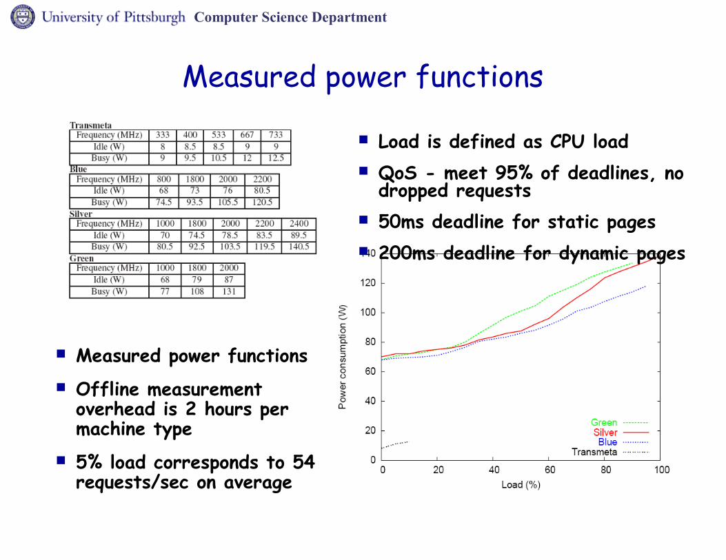
Measured power functions

Load is defined as CPU load QoS - meet 95% of deadlines, no

dropped requests 50ms deadline for static pages 200ms deadline for dynamic pages

Measured power functions Offline measurement

overhead is 2 hours per machine type

5% load corresponds to 54 requests/sec on average


Servers– Process requests, return

results– Local power management– Monitor, feedback load

request

server pool

front endrequest

distribution

result

feedback

Front end– Request distribution– Load balancing– Global power management

Clients

Global PM – server clusters


Homogeneous clusters - LAOVS

Load-aware on/off

DVS locally

Load estimated online

Offline computed table servers versus load

PPC750 cluster (2 nodes) implementation

4x savings over noPM

noPM

With PM


Heterogeneous clusters – global PM

Two tables determine #servers as a function of load Servers are turned on/off in power efficiency order (fixed) Low overhead (microseconds) – can be computed online

mandatory_servers[i] – records the load at which server i must be turned on to satisfy the QoS Turn on new server when existing servers cannot handle load If server 0 can handle 100 reqs/sec and server 1 handles 200

reqs/sec, turn on server 2 when rate reaches 300 reqs/sec If it takes 10 seconds to boot and max load increase is 5

reqs/sec, turn on server 2 when load reaches 250 reqs/sec Power consumption not considered


Power-aware on/off

power_servers[i] – records the load at which i servers become more energy efficient than i-1 servers Efficient procedure (microseconds) computes the table by

escalating the power functions Example : server A currently at 5mW/request, server B at

6mW/request -> server A wins the request and moves up in the power curve (say at 5.3mW)

Periodically Estimate load, turn on mandatory servers if necessary Turn on/off one server at a time (if possible) to reduce power Rent-to-own thresholds consider boot and shutdown times


Global power management - evaluation

For fairness, all schemes use the energy-aware request distribution policy

45% energy savings on average

DVS has less of an impact due to high idle power in our servers

QoS above 99% for all points

cluster power vs load


More flexible cluster with Power Mgmt?

The cluster approach is somewhat static, not accounting for too much variability on the average execution time of requests on definition of QoS

A more dynamic server handles such variability automaticallyFor example, using control theoryMeasure tardiness and control speed directly

proportional to tardiness


Web Interaction Response Time (WIRT)

Client DB serverFront-end Server node

PHP Requestproxy

DB accesses

HTML response with embedded objects

Embedded objects requests

Embedded objects

Web

inte

ract

ion

resp

onse

tim

e

(WIR

T)

To any server node


Measuring end-to-end time delay

Client Front-endServer node 1

Server node 2

Server node 3

req.phpreq.php?r=123

Img1.jpg?123

Img3.jpg?123

Img2.gif?123

img1.jpg?123

img2.gif?123

img3.jpg?123

WIR

T


QoS Metric / Control Variable

Main idea: control system

Actuate on the frequency (and voltage) of CPU

Measure/sense the tardiness

PID Controller



Pr [ tardiness≤ x ]=p

x → p-quantile

PID Controller [FeBID 2007]:



Pr [ tardiness≤ x ]=p

x → p-quantile

PID Controller [FeBID 2007]:


MULTI PROCESSORS


Types of Applications:AND/OR Applications on Multiprocs

Tasks Set of independent tasks Time budget (Desired

completion time)

Directed Acyclic Graph (DAG) Comp. (ci, ai) AND (0,0) OR (0,0): probabilities

T1

T2 T3 T4 T5

(1,2/3)

(2,1) (1,1) (4,2) (3,2)

T7

T6

(1,1)

(1,1)

60% 40%

The Example

Ti


Global, Dynamic Power Management forReal-time with firm Deadlines

Greedy may cause scheduling anomalyAny available slack is given to next ready taskFeasible for single processor systemsFails for multi-processor systems

ba c fed

time

b

a

D

d e

fcMiss

time

b

a

D

c

d e fSlack


Slack Stealing

Shifting Static Schedule: 2-proc, D = 8

0 1 2 3 4 5 6 7 8 time

f

T1

T4

T5

T7

D

L0

T1

T4

T5

T7

f

0 1 2 3 4 5 6 7 8 time

Shifting

D

L0

T3

T2 T6L1

Recursive if embedded OR nodes

T3

T2 T6

T1T7

`L1


Greedy algorithm, two phases

Off-line: longest task first heuristic; Slack stealing via shifting heuristic

On-line:Same execution orderClaim the slack: Compute speed:

If c= WCET, meet timing requirementIf c= ACET, good also for regular systems

f gi =f max×

c i

ci+Slack i


Actual Running Trace

Actual Running Trace: left branch, Ti use ai

Possible ShortcomingsNumber of Speed change (overhead)Too greedy: slow fast

T7

f

0 1 2 3 4 5 6 7 8 time

D

T6

T1

L0

T3

T2

L1


Optimal for uniprocessor: Single speed Energy – Speed: Concave Minimal Energy when all tasks SAME speed

Speculation: statistical information about Application Static Speculation

All tasksfi = max ( fss, fg

i)

Adaptive SpeculationRemaining tasksfi = max ( fas, fg

i)

Speculation works for both RT and non RT

f ss=waverage

all

D

f as=waverage

remaining

timer

More Algorithms


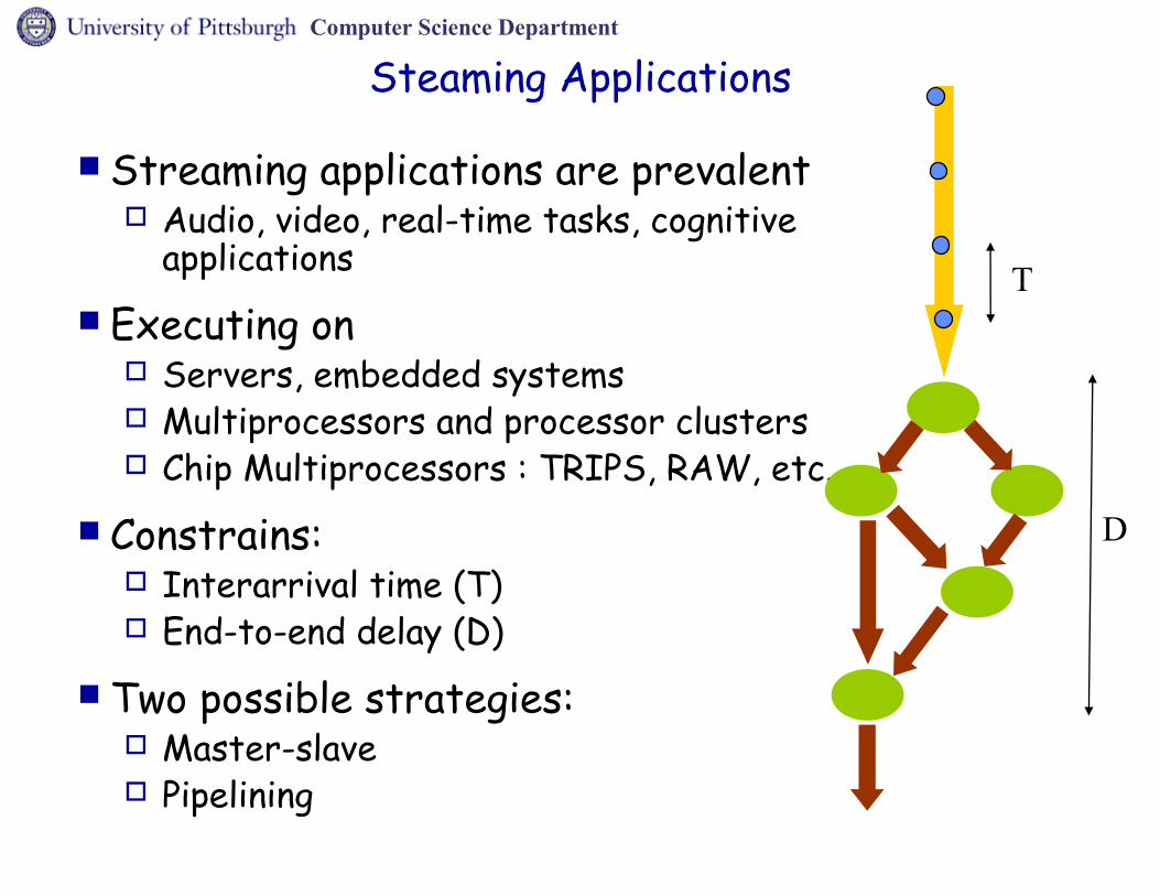
Steaming Applications

Streaming applications are prevalent Audio, video, real-time tasks, cognitive

applications Executing on

Servers, embedded systems Multiprocessors and processor clusters Chip Multiprocessors : TRIPS, RAW, etc.

Constrains: Interarrival time (T) End-to-end delay (D)

Two possible strategies: Master-slave Pipelining

T

D


Master-slave Strategy

Single streaming applicationThe optimal number, n, of active PEs

strikes a balance between static and dynamic power

Given n, the speed on each PE is chosen to minimize energy consumption

Multiple steaming applicationsDetermine the optimal number of

active PEsGiven the number of active PEs,

First assign streams to groups of PEs (ex: balance load using the minimum span algorithm).

Adjust the speed on each PE to minimize energy

PEPE

PEPE

PEPE

PEPE

TT

DD


Pipeline Strategy

(1) Linear pipeline (# of stages = # of PEs)

PEPE PEPE PEPE PEPE


Pipeline Strategy

(2) Linear pipeline (# of stages > # of PEs)

PEPE PEPE PEPE PEPE

Solution 1 (optimal)Discretize the time and use dynamic

programming

Solution 2 (use some heuristics)

(3) Nonlinear pipeline # of stages = # of PEs

Formulate an optimization problem with multiple sets of constraints, each corresponding to a linear pipeline

Problem : the number of constraints (can be exponential)Solution : add additional variables denoting the finishing

time for each stage

# of stages > # of PEsApply partitioning/mapping first and then do power

management


A

B C

D

E F G H I

J

A

B C

D

E F

G H I

J

Level 1

Level 2

Level 3

Level 4

Level 5

Stage 1

Stage 2

Stage 3

• Step 1: topological-sort-based morphing• Step 2: A dynamic programming approach to find the optimal # of stages and optimal # of processors for each stage

Scheduling into a 2-D processor array (CMP)


Tradeoff: Energy & Dependability


Time slack (unused processor capacity)

Power management Fault tolerance Increase productivity

Use to reduce speed Use for redundancy Use to do more work

Timeredundancy

Spaceredundancy

Effect of DVSon reliability


Exploring time redundancy

The slack is used to:1) add checkpoints 2) reserve recovery time 3) reduce processing speed

For a given slack and checkpoint overhead,We can find the number of checkpoints and the placement of checkpointsSuch that we minimizes energy consumption, and guarantee recovery and timeliness.

# of checkpoints

Ener

gy


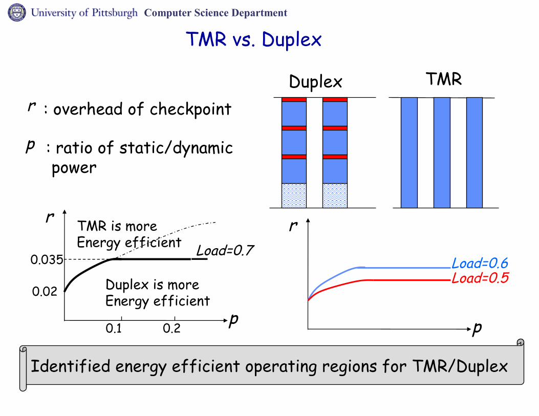
TMR vs. Duplex

TMRDuplex

Load=0.6

r

Load=0.5

Identified energy efficient operating regions for TMR/Duplex

Duplex is more Energy efficient

TMR is more Energy efficient

0.02

0.035Load=0.7

p p

r

p

r

0.1 0.2

: overhead of checkpoint

: ratio of static/dynamic power


Effect of DVS on SEU rate

Lower voltages higher fault rate Lower speed less slack for recovery

Faultmodel

Reliabilityrequirement

Availableslack

Acceptable level of DVS


Energy Savings throughCommunication


Energy savings in communication links

put here some information on comm links energy modelsWireless (just to mention or maybe remove it)

Power proportional to Distance Power proportional to encoding

Wired Predicting communication patters can allow for

slowing down or turning off links, routers, etc without much penalty in performance

Using buffered networks can allow for ???


Saving Power in Wireless

Power is proportional to the square of the distance

The closer the nodes, the less power is needed Power-aware Routing (PARO) identifies new

nodes “between” other nodes and re-routes packets to save energy

Nodes decide to reduce/increase their transmit power


Asymmetry in Transmit Power

Instead of C sending directly to A, it can go through B

Saves transmit power, but may cause some problems.

AB

C

AB

C


Problems due to one-way links.

Collision avoidance (RTS/CTS) scheme is impaired Even across bidirectional links!

Unreliable transmissions through one-way link. May need multi-hop Acks at Data Link Layer.

Link outage can be discovered only at downstream nodes.

A B C

RTSCTS CTS

MSG MSG MSG


Problems for Routing Protocols

Route discovery mechanism. Cannot reply using inverse path of route request. Need to identify unidirectional links. (AODV)

Route Maintenance. Need explicit neighbor discovery mechanism.

Connectivity of the network. Gets worse (partitions!) if only bidirectional links are

used.


Wireless bandwidth and Power savings

In addition to transmit power, what else can we do to save energy?

Power has a direct relation with signal to noise ratio (SNR)The higher the power, the higher the signal, the less

noise, the less errors, the more data a node can transmit

Increasing the power allows for higher bandwidth Turn transceivers off when not used – this

creates problems when a node needs to relay messages for other nodes.


SAVING ENERGY WITH COMMUNICATION


Communications Links

Use of “serial” links is spreadingHigher performanceEasier to manufacture for longer distances

Used in a variety of situations:Intersystem

Ethernet, infiniband, others.Multiple speeds available but fixed after initial configuration

(like some memory)

IntrasystemSATA (3Gbps), PCIe (2.5, 5 and 8Gbps)

Higher speed = higher power


Communication Links: intrasystem

Intrasystem serial links are more numerous increasing its share in system power


Communication Links: intrasystem

Each link has 2 transceivers A system may contain hundreds of transceivers: 50 PCIe lanes

are available in some systems


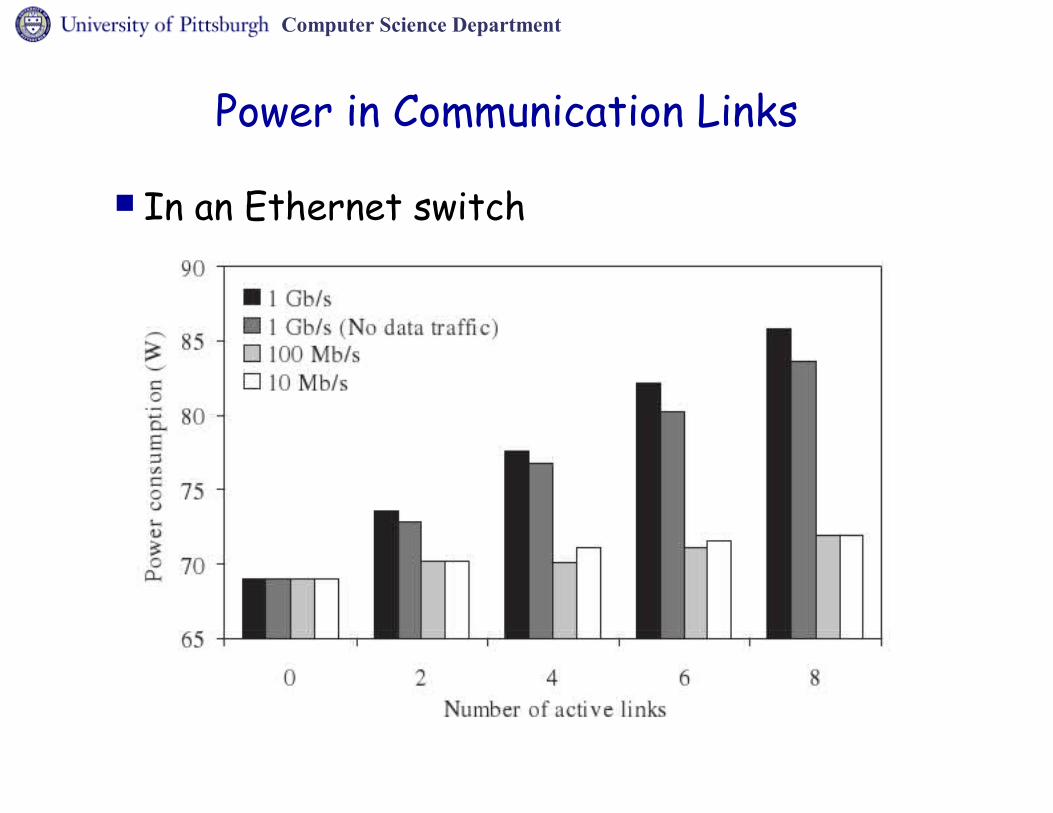
Power in Communication Links

In an Ethernet switch


Power in Communication Links - II

In an desktop environment:1Gbps → 100Mbps can save up to 4W100Mbps → 10Mbps saves up to 0.5W


Communication Patterns in Supercomputers

Many HPCS applications have only a small degree (6-10) of high bandwidth communication among processes/threads

Rest of a thread’s / process’ communication traffic are low bandwidth communication “exceptions”.

Many HPCS applications have persistent communication patterns

Fixed over all the program’s run time, or slowly changing

But there are “bad” applications, or phases in applications, which are chaotic


The OCS Network fabric

Fat-tree networkFat-tree networkFat-tree networkFat-tree networkFat-tree networkFat-tree networkFat-tree networkOne of multiple fat-tree networksOne of multiple fat-tree networksOne of multiple fat-tree networksOne of multiple fat-tree networksOne of multiple fat-tree networksOne of multiple fat-tree networksOne of multiple fat-tree networksOne of multiple fat-tree networks

Circuit-Switched all Optical Fat-Trees made of 512x512 MEMS-based optical switches

Intelligent Network (1/10 or less BW)Including collective communication

Storage/IO NetworkPERCS D-block PERCS D-block

2 networks complement each other

OCS


Communication Phases

(Node 48)

250 sec phase

Communication Pattern: node48 AMR CTH

Communication patterns change in phases lasting 10’s of Sec

50 sec phase

60 sec phase

30 sec


10

100

1

Max communication degree from each node to any other node is about 10. The pattern

is irregular but fixed.

>60%40% to 60%20% to 40%0% to 20%No communication

Communication Matrix

UMT2K – Fixed, Irregular Communication Pattern

Percentage of Traffic By Bandwidth


NOTE: No changes in the application code

HPCS applications

Low High

Compile TimeStatically Analyzable

Run-Time Predictable

Un-Predictable

Temporal Locality

CommunicationUn-predictability

Use multiple hops through OCS

ORuse intelligent

network

Communication

CompiledCommunication

Run-time predictor


Paradigm of compiled communication

CompilerMPI application

CommunicationPatterns

MPI trace code

Optimized MPIcode

Network configuration

Instruction Enhanced MPI code

NetworkConfigurations

HPC systems Traces

Compiled communication Performance

statisticsHPC systems (Simulator)

Run-time predictor


Compilation Framework

Compiler: Recognize and represent

communication patterns Communication compiling

Enhance applications with network configuration instructions

Automate trace generation

Targets MPI applications


Communication Pattern

phase

phase

phase

Communication Classification:Static PersistentDynamic

Executions of parallel applications show communication phases


The Communication Predictor

• Initially, setup the OCS for random traffic

• Keep track of connections’ utilization

• A migration policy to create circuits in OCS

•A simple threshold policy•An intelligent pattern predictor

• An evacuation policy to remove circuits from OCS

•LRU replacement •A compiler inserted directive

router

Intra D-Block

NIC

Inter D-Block:High Bandwidth Optical Network

OCScontrol

CommunicationPredictor

NICLow BWNetwork

Processor Node


Example: Route from node 2 to node 4 (second node in second group)

0

1

2

3

4

5

6

7

8

0

1

2

3

4

5

6

7

8

0

1

2

3

4

5

6

7

8

0

1

2

3

4

5

6

7

8

Dealing with Unpredictable Communications

Set up the OCS planes so that any D-block can reach any other D-block with at most two hops through the network

1) Route from node 2 to node 7

2) Route from node 7 to node 4


Scheduling in Buffer Limited Networks

Collaborators :Taieb Znati

PhD student:Mahmoud Elhaddad


Packet-switched Network with Fixed-Size Buffers

Packet routers connected via time-slotted buffer-limited links Packet duration is one slot You cannot freely size packet buffers to prevent loss

All-optical packet routers On-chip (line-driver chip) SRAM buffers

Connections: Ingress--egress traffic aggregates Fixed bandwidth demand Connection has fixed path

Loss rate of a connection Loss rate is fraction of lost packets goal is to Guarantee loss rate

Loss guarantee depends on the path of connection


Link scheduling algorithms

Packet Service discipline: FCFS, LIFO, Fixed Priority, Nearest To Go…

Drop policy: Drop tail, drop front, random drop, Furthest To Go…

Must be Work conserving: Drop excess packets only when buffer overflows Serve packet in every slot as long as buffer not empty

Must use only local information No hints or coordination between routers


Link scheduling in buffer-limited networks Problem:

Minimize guaranteed loss rate for every connectionKey question: Is there a class of algorithms that lead

to better loss bounds as fn of utilization and path length?

FCFS scheduling with drop tail Proposed rolling priority scheduling


Link scheduling in buffer-limited networks

Findings:A local fairness property is necessary to minimize the

guaranteed loss rate for every path length and utilization constraint.

FCFS/RD (Random Drop) is locally fair

A locally-fair algorithm Rolling Priority that improves the loss guarantees compared to FCFS/RD, and is simple to implement

Rolling Priority is optimalFCFS/RD is near-optimal at light load


Rolling Priority Time divided into epochs of fixed duration nT.

Connection Initialization: Ingress chooses a phase at random from the duration of an epoch. At t+offset, ingress sends an init packet along the path of

connection Init packets are rare and never dropped

At every link, a new epoch starts periodically

At each time slot, every link gives higher priority to the connection with earlier starting current epoch.


Thermal stuff!


Thermally-aware computing

CPU thermal models at architectural levelHotSpot [Skadron HPCA 2002]Server thermal model, DVS and failures are not

considered Real-time temperature-aware scheduling, only CPU

considered [Bettati RTSS-2006,ECRTS-2006]Temperature minimization algorithms [Chen RTAS-2007]

Datacenter Thermal Management: Server as a black box [Chase Usenix 2005]

Thermal simulator and Load-balancing: Mercury and Freon [Bianchini Rutgers 2005]

DVS is not considered Model addressing failures of cooling devices [Ferreira

ECRTS 2007]


A Thermal ModelVery simple model

Has a equivalence to an electric RC model

Low computational overheadAggregation of elementsWhole components represented by a very small number

of resistors and capacitors But less accurate than more complex models

Current Charge Voltage Resistance Capacitance Current source

Heat TransferHeatTemperatureThermal resistanceThermal capacitanceHeat producer


New Thermal ModelModel addresses failures of cooling devices

Usability:

SimulationHard to do real experimentsEven harder for larger systemsLow repeatability of real experiments

On-line resource managementAdmission controlThermal-Aware Load-balancing


Use electrical equations, due to similarity System of linear first degree differential equations

It can predict the dynamic behavior of the system (i.e., temperature prediction)

System is stable – does not oscillate

RC Models Equivalence


The 2J/°C box capacitance was changed to 20J/°C. This change the time constant from 20s to 200s

Initial conditions: TCPU

= 50°C, TBOX

= 20°C

This model shows effect of an capacitance in the dynamic behaviour of the system.


Thermal ModelExample - Low Capacitance 2J/°C

Exponential with both achieving stable temperature at same time


Thermal ModelExample - High Capacitance 20J/°C

Dominated by CPU capacitance (small)

Dominated by BOX capacitance(BIG)

CPU maintains constanttemperature difference


More complex model Thermal capacitances

are very different � time constants will be very different.

Thermal resistances are comparable temperature differential will be similar.

Silicon Chip

ThermalCompoundChip-Metal Lid

Metal Case

ThermalCompoundMetal Lid-Heatsink

HeatFlow

CPU Thermal Model


Disk Thermal Model

Simple model used Only considering the external disk case temperature


Complete Server Thermal Model

Switches represent value change when a failure occurCPU fanCase fan

External failures are represented by an increase of ambient temperature


Rack Thermal Model

ServerUses the presented model

RackConstant temperature

source of 25°CAssumed air-conditioned

with constant temperature. It is a current sink or source.


Simplified model but accurate for slow temperature variations.

Components to be modelled:Case, disks, CPU and rack

Server Thermal Model


Model ValidationExperimental Setup

Server specifications Hardware

Athlon64 3000+ with 512KB cache using AMD coolerHas an internal temperature sensor available via lm_sensors

1GB RAM - DDR PC3200 Motherboard Abit KN8 with chipset Nforce 3

Chipset also has an internal temperature sensor available via lm_sensors

80GB PATA drive + DVD-ROMDesktop case

Has a temperature sensor and an external LCD display Software

Gentoo Linux 2006.0 - kernel 2.6.16-gentoo-r9 lm_sensors-2.10


Model ValidationParameters Determination

Use physical properties to estimate valuesCapacitance

Type of materialMass

Resistance (much harder to estimate)Type of materialShapeSizeUsed similar components values when available

Compared with measurements from actual system


ValidationTemperature x Power Model (Steady state)


Validationload 0 100%→

Exponential relationship temperature x time Very long time constants


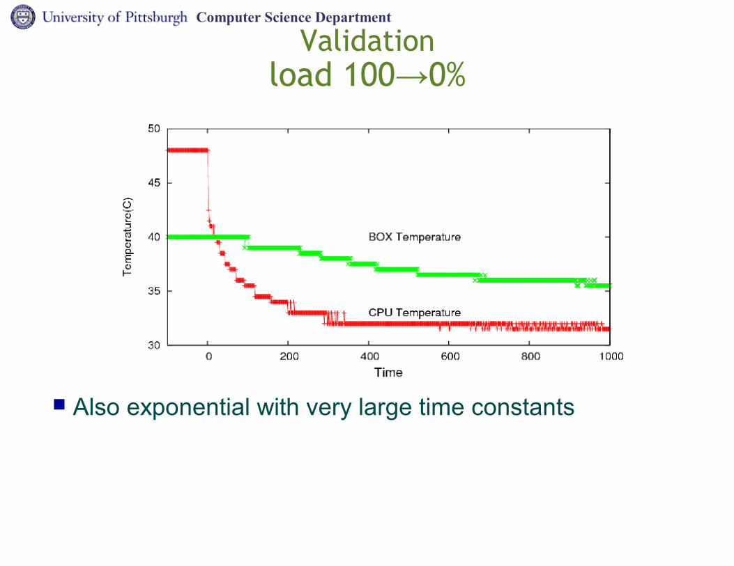
Validationload 100 0%→

Also exponential with very large time constants


CPU fan failure at time 4000.

Heat transfer is less efficient so even with no load it takes a longer time to return to normal temperature

RC Thermal Model Simulating Failure


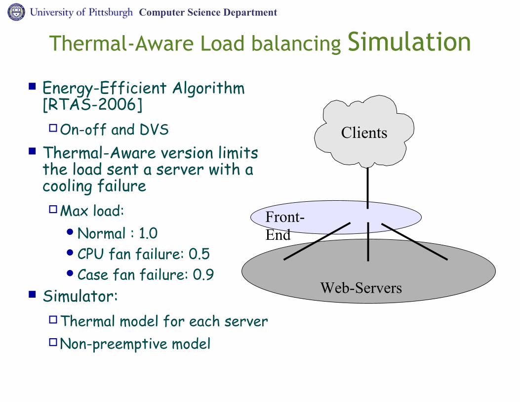
Energy-Efficient Algorithm [RTAS-2006]On-off and DVS

Thermal-Aware version limits the load sent a server with a cooling failureMax load:

Normal : 1.0CPU fan failure: 0.5Case fan failure: 0.9

Simulator:Thermal model for each serverNon-preemptive model

Thermal-Aware Load balancing Simulation

Clients

Front-End

Web-Servers


Thermal-Aware Load balancing Single Server Power Model

Linear relationship Load versus Power for a single frequency

Quadratic Power versus Frequency (Constant load) DVS allows to use a reasonable fraction of a server

capacity even when having a cooling failure


Thermal-Aware Load balancing Farm Power Model

All thermal faults are modelled at server 0 (first server to be used)

High temperature achieved with no thermal-awareness

Thermal-Aware turn-on new server earlier reducing the load on affected server


Thermal-Aware Load balancing Dynamic Behaviour

Server 0 has a CPU fan failure at 600s with 0.6 load applied to the system

Server 1 is turn-on to reduce load on server 0

Division is asymmetric because the algorithm uses the lowest power configuration

Even though temperature rises on CPU 0 it stays within design limits


Bibliography D. Zhu, R. Melhem and D. Mossé. The Effects of Energy Management on Reliability in Real-Time Embedded

Systems; to appear in International Conference on Computer Aidded Design, Nov. 2004D. Marculescu. On the Use of Microarchitecture-Driven Dy namic Voltage Scaling. In Proceedings of the Workshop on Complexity-Effective Design, in conjunction with ISCA-27, June 2000.

N. AbouGhazaleh, D. Mossé, B. Childers, R. Melhem, "Collaborative Operating System and Compiler Power Management for Real-Time Applications", ACM Trans. on Embedded Computing Systems (TECS), February 2006, Vol.5, issue1.

Chamara Gunaratne, Ken Christensen*,† and Bruce Nordman, “Managing energy consumption costs in desktop PCs and LAN switches with proxying, split TCP connections, and scaling of link speed”, Int. J. Network Mgmt 2005; 15: 297–310 Published online in Wiley InterScience (www.interscience.wiley.com). DOI: 10.1002/nem.565

Ganesh Balamurugan,, Joseph Kennedy, Gaurab Banerjee, James E. Jaussi,, Mozhgan Mansuri, Frank O’Mahony, Bryan Casper, and Randy Mooney, “A Scalable 5–15 Gbps, 14–75 mW Low-Power I/O Transceiver in 65 nm CMOS” , IEEE Journal of Solid-State Circuits, vol. 43, no. 4, April 2008

“Low Power Server CPU Shoot-out”, http://www.anandtech.com/IT/showdoc.aspx?i=3039&p=1

http://www.top500.org

http://www.green500.org

“AMD Firestream”, http://ati.amd.com/products/streamprocessor/specs.html

“Nvidia Tesla”, http://www.nvidia.com/object/tesla_computing_solutions.html

“Intel ATOM benchmarked”, http://www.anandtech.com/showdoc.aspx?i=3321&p=1

http://www.anandtech.com/IT/showdoc.aspx?i=3039&p=1



http://www.top500.org/

http://www.green500.org/

http://ati.amd.com/products/streamprocessor/specs.html

http://ati.amd.com/products/streamprocessor/specs.html

http://www.nvidia.com/object/tesla_computing_solutions.html

http://www.nvidia.com/object/tesla_computing_solutions.html


Bibliography K. Skadron, M. Stan, M. Barcella, A. Dwarka, W. Huang, Y. Li, Y. Ma, A. Naidu, D. Parikh, P. Re, G. Rose, K.

Sankaranarayanan, R. Suryanarayan, S. Velusamy, H. Zhang, and Y. Zhang. HotSpot: Techniques for Model-ing Thermal Effects at the Processor-Architecture Level. In International Workshop on THERMal INvestigations of ICs and Systems, 2002.

S. Wang and R. Bettati. Delay Analysis in Temperature-Constrained Hard Real-Time Systems with General Task Arrivals. In IEEE Real-Time Systems Symposium (RTSS)., 2006.

S. Wang and R. Bettati. Reactive Speed Control in Temperature-Constrained Real-Time Systems. In Euromicro Conference on Real-Time Systems (ECRTS), 2006.

J. Chen, C. Hung, and T. Kuo. On the Minimization of the Instantaneous Temperature for Periodic Real-Time Tasks. In IEEE Real-Time and Embedded Technology and Applica tions, 2007.

J. Moore, J. Chase, P. Ranganathan, and R. Sharma. Making Scheduling Cool¨ Temperature-Aware Resource Assignment in Data Centers. In Usenix Annual Technical Conference, 2005.

T. Heath, A. Centeno, P. George, L. Ramos, Y. Jaluria, and R. Bianchini. Mercury and freon: Temperature emulation and management for server systems. In Conference on Architectural Support for Programming Languages and Operating Systems, 2006.

Alexandre P. Ferreira, Daniel Mossé and Jae C. Oh, Thermal Faults Modeling using a RC model with an Application to Web Farms. In Euromicro Conference on Real-Time Systems (ECRTS), 2007.

Documents

Power management in XX systems XX = real-time | …varsha/allpapers/power-aware...Computer Science Department Basics of Energy and Power Power (P) consumption is proportional to the