Power-laws, persistence and the distribution ofinformation in software systems

Les HattonCISM, University of Kingston∗

January 12, 2010

Abstract

In a previous paper, an intimate link between power-law distribu-tion in the tail of component sizes and defect appearance in maturingsoftware systems, independently of their representation language, wasrevealed by the use of a variational method built on statistical me-chanical arguments.

Building on the above work, this paper first of all demonstrates ex-perimentally that power-law behaviour in the tail of component sizesappears to be a persistent property in that it is present from the ear-liest release of software systems. It then develops a model for thisbehaviour by combining statistical mechanics with a modification ofHartley/Shannon information content to predict power-law behaviourin the alphabet of tokens used in programming languages; the ap-proximate linearity of user-defined variable names with componentsize, and finally, that defects will also obey a power-law, leading di-rectly to a prediction of defect clustering. Each of these is supportedby good experimental evidence across numerous systems. The modeltherefore unifies the distribution of information content through thedevelopment process with the appearance of power-law behaviour inalphabet and consequently, component size as well as the distributionof defects in the release phase.

Keywords: Information content, defect clustering,

Component size distribution, Power-law

∗L.Hatton@kingston.ac.uk, lesh@oakcomp.co.uk

1

1 Background

In [10], a model based on statistical mechanics was presented which showedthat, in a software system subject only to the twin constraints of total size andnumber of defects present a priori, a component size distribution exhibitingpower-law behaviour in medium to large components (i.e. greater than about20 executable lines of code (XLOC)) was inextricably linked with a growthin defects within a component of xlogx where x is the number of XLOC.Numerous systems in several different languages were also analysed to showthat such power-law behaviour in component size was indeed present. Thepaper concluded by saying that it was not however clear which if either ofthese two phenomena was the driver.

The current paper builds on this work and makes a number of furthercontributions.

• First, it demonstrates using further experimental evidence that power-law behaviour in the tail of component sizes in disparate software sys-tems is a persistent property in that it appears to be present from theearliest days of a released software system. In other words, it appearsto evolve naturally during development driven perhaps by some deeperprinciple. This sets the scene for what follows.

• Second, it provides a mechanism which explains the natural appearanceof power-law size distributions during development, independently ofany representation. The resulting model is a novel modification of theHartley / Shannon information content within a variational context.This model also attempts to explain observed departures from power-law in smaller components. This phenomenon is demonstrated usingmajor systems.

• Third, it demonstrates that this leads to an approximate linearity be-tween user-defined variable names and component size in executablelines of code. This is demonstrated in real systems.

• Fourth, it then unifies this model with that presented in [10]. It is thenable to predict that defects will cluster. This is also illustrated withexamples from real systems.

2

2 Power-law behaviour

For reference, power-law behaviour can be represented by the probabilityp(s) of a certain size s appearing being given by a relationship like:-

p(s) =k

sα(1)

where k is a constant, which on a log p - log s scale is a straight line withnegative slope.

Power-law behaviour has been studied in a very wide variety of environ-ments, see for example [21] (economic systems) and the excellent review by[19]. In software systems there has been significant activity, much of it recent,[5], [18], [17], [3], [7], [20], [1], [6] and [10] all discuss power-law behaviourbut in rather different contexts. Of these, both Mitzenmacher [17], and Gor-shenev and Pis’mak [7], are particularly relevant to the present work.

Mitzenmacher considers the distributions of file sizes in general filing sys-tems and observed that such file sizes were typically distributed with a log-normal body and a Pareto (i.e. power-law) tail. This does not howeverconflict with the present work as it also leads to a Pareto tail. Perhaps moreimportantly, his work dealt with sizes in general file systems rather thanthe symbols of distinct software packages containing numerous strongly re-lated files, together providing the functionality of the software package. Thisdistinction may also be relevant but has not been pursued further here.

Gorshenev and Pis’mak studied the version control records of a number ofopen source systems with particular reference to the number of lines addedand deleted at each revision cycle. The relevance of this will be discussedshortly.

Given the observed appearance of power-law behaviour in such componentsizes reported in numerous software packages of very different provenance by[10], and its central part in the theoretical development both there and here,it is of particular interest to investigate why and when such behaviour wouldemerge, given its link with defect behaviour within components.

Newman in his comprehensive review of power-law behaviour [19], de-scribes a number of potential generating mechanisms.

• Inverses of quantities

3

• Random walks

• The Yule process

• Phase transitions

• Self-organised criticality

• Combinations of exponentials

Of these, the last named will prove particularly useful in the developmentwhich follows.

2.1 Some notes on data presentation and averaging

Before presenting any evidence, it is worth mentioning in passing that soft-ware data is typically very noisy for a variety of reasons. Factors of 10 ormore between developers in the same group are often noted by researchers inmeasuring various parameters, for example fault detection capability duringinspections, [9]. Furthermore, in comparisons of software components writ-ten independently to the same specification even in the same programminglanguage, significant variations in program size measured in lines of codehave similarly been reported, [15], [25]. This means that sometimes signifi-cant smoothing is necessary to reveal any systematic patterns amongst theinevitable noise. Where necessary in this paper, the arithmetic mean is usedwithout further massaging and its use will be pointed out as appropriate.

With regard to the number of case studies presented in support of each ofthe testable predictions made, the case studies were chosen at random and(with one exception), at least four very different datasets were used for eachas a compromise between shortage of space and statistical reasonableness.For the central result of the paper, six were used.

The systems analysed include large systems worked on by many program-mers over a long period, (including the X11R5 library and server, NAGFortran and C libraries), medium-sized systems worked on for timescalesup to 20 years by teams of up to 10, (commercial embedded system, datavisualisation, GNU assembler) and many versions of medium-sized systemsworked on by one or two developers, (Tcl-Tk GUIs and parsing systems), ontimescales up to 10 years.

4

2.2 Persistence of power-law behaviour in size distri-butions

In [10], amongst other things, strong evidence of power-law behaviour inthe tail of component size distributions for 21 systems of very different size,provenance and programming language is presented. A natural questionto ask wherever this information is available, is if this behaviour is persis-tent from the time of the first release, or whether the power-law behaviouremerged subsequent to its first release as the system matured. If power-lawbehaviour is present from the earliest days of a released system presumablyas a result of some underlying principle acting during development, then themathematical relationship in [10] predicts that this will act as a driver suchthat defect growth in a component proportional to xlogx is most likely to takeplace as the system matures, where x is the number of XLOC. Indeed, someevidence for this functional defect growth was presented using mature sys-tems data but the question remains open whether the power-law behaviouris indeed persistent.

Practical considerations suggest that it would be unusual to expect ma-jor changes in component size distribution as a system ages on the generalgrounds that engineers are reluctant to change working systems too mucheven as they adapt to changing requirements and other normal maintenanceactivities. By good fortune, several of the 21 systems analysed in [10] hadsource revision history, two from the very first release of 7-8 year life-cyclesand one from around half way into its 25 year life-cycle from first release.These three systems are highly disparate but to broaden the relevance, anearly and a late version of the data visualisation program xgobi / ggobi ([24]),were also analysed.

To reduce the noise in showing the component-size distributions for eachrelease, the data are displayed using the cumulative distribution methoddescribed by [19]. Here the shape of the distribution is irrelevant, it is thechange in shape across revisions which is of particular note. If this does notchange substantially, then power-law behaviour in the tail is persistent, sincein each case, it was present in the latest releases.

Relevant parameters of these four packages are shown as Table 1.

5

Package Language releases Years start XLOC end XLOC

Numerical li-brary

Fortran 8 12 90,198 266,123

Geophysicalmodelling

Tcl-Tk 44 7 6,227 11,078

Language parser C 27 8 35,851 65,270Visualisation C 2 shown 17 ∼ 12, 000 ∼ 48, 000

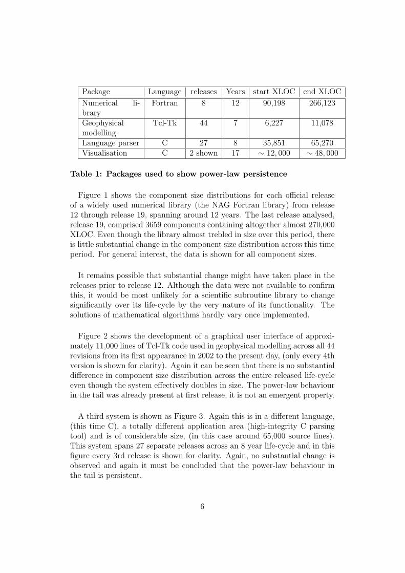
Table 1: Packages used to show power-law persistence

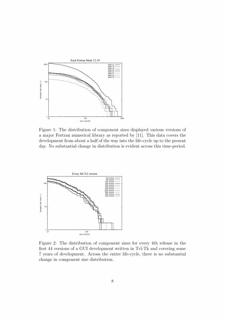
Figure 1 shows the component size distributions for each official releaseof a widely used numerical library (the NAG Fortran library) from release12 through release 19, spanning around 12 years. The last release analysed,release 19, comprised 3659 components containing altogether almost 270,000XLOC. Even though the library almost trebled in size over this period, thereis little substantial change in the component size distribution across this timeperiod. For general interest, the data is shown for all component sizes.

It remains possible that substantial change might have taken place in thereleases prior to release 12. Although the data were not available to confirmthis, it would be most unlikely for a scientific subroutine library to changesignificantly over its life-cycle by the very nature of its functionality. Thesolutions of mathematical algorithms hardly vary once implemented.

Figure 2 shows the development of a graphical user interface of approxi-mately 11,000 lines of Tcl-Tk code used in geophysical modelling across all 44revisions from its first appearance in 2002 to the present day, (only every 4thversion is shown for clarity). Again it can be seen that there is no substantialdifference in component size distribution across the entire released life-cycleeven though the system effectively doubles in size. The power-law behaviourin the tail was already present at first release, it is not an emergent property.

A third system is shown as Figure 3. Again this is in a different language,(this time C), a totally different application area (high-integrity C parsingtool) and is of considerable size, (in this case around 65,000 source lines).This system spans 27 separate releases across an 8 year life-cycle and in thisfigure every 3rd release is shown for clarity. Again, no substantial change isobserved and again it must be concluded that the power-law behaviour inthe tail is persistent.

6

The fourth system is shown as Figure 4. Although again in C, this is thewell-known visualisation system xgobi / ggobi, [24] and again no evidenceof substantial change in component size distribution is evident across the 17years separating these two versions during which time the system increasedin size by a factor of four.

Given the very disparate nature of these four systems, it can be tenta-tively concluded that component size distributions do not appear to changesubstantially across long life-cycles of medium to large packages, (here therange is 11,000 - 270,000 XLOC in three different languages and very differ-ent application areas). In other words, the power-law behaviour in the tailsof component sizes is a persistent property, present at first release and it doesnot emerge during the maintenance cycle, even when that doubles, triples oreven quadruples the initial released system size as is the case here.

This paper will now attempt to answer why such behaviour appears tobe persistent. Gorshenev and Pis’mak [7] address a related problem, thatof explaining why the added and deleted code in an evolving system shouldobey a power-law distribution. To this end, they use a model of softwareevolution based on natural selection. Here, a somewhat different problemis being addressed, that of explaining why power-law behaviour in the tailappears to be present from a system’s first release. To this end, an entirelydifferent approach will be taken based around information content.

3 A mechanism for persistence

To be present in the first release of such disparate systems, it is obvious thatany such power-law behaviour must evolve naturally as the functionality ofa system is implemented in a software context during development and musttherefore be intimately related to that functionality in some sense and thiswill be pursued here.

Historically, functionality has proven to be an elusive goal to quantifyfor computer scientists as evidenced by the fact that the number of linesof code still appears to be the dominant measure of size, and by commonassociation, functionality, even though a line of code is itself a somewhatarbitrary measure, strongly related to the implementation language and alsothe developer’s personal taste. In addition, different alternatives presentthemselves, for example, in C and C++, the following are all used:-

7

1

10

100

1000

10 100 1000

Sam

ple

s w

ith v

alu

e >

x

size x (XLOC)

Each Fortran Mark 12-19

Mark 12Mark 13Mark 14Mark 15Mark 16Mark 17Mark 18Mark 19

Figure 1: The distribution of component sizes displayed various versions ofa major Fortran numerical library as reported by [11]. This data covers thedevelopment from about a half of the way into the life-cycle up to the presentday. No substantial change in distribution is evident across this time-period.

1

10

100

10 100

Sam

ple

s w

ith v

alu

e >

x

size x (XLOC)

Every 4th Tcl version

4th version8th version

12th version16th version20th version24th version28th version32nd version36th version40th version44th version

Figure 2: The distribution of component sizes for every 4th release in thefirst 44 versions of a GUI development written in Tcl-Tk and covering some7 years of development. Across the entire life-cycle, there is no substantialchange in component size distribution.

8

1

10

100

1000

10 100 1000

Sam

ple

s w

ith v

alu

e >

x

size x (XLOC)

Every 3rd C version

1st version4th version7th version

10th version13th version16th version19th version22nd version25th version

Figure 3: The distribution of component sizes displayed for every 3rd releasein the first 27 versions of a high-integrity parsing engine written in C andcovering some 8 years of development. Across the entire life-cycle, there isno substantial change in component size distribution.

1

10

100

1000

10 100 1000

Sam

ple

s w

ith v

alu

e >

x

size x (XLOC)

xgobi versions separated by 17 years

1992 version2008 version

Figure 4: The distribution of component sizes displayed for two releases ofthe xgobi/ggobi visualisation engine separated by 17 years. Across the entirelife-cycle, there is no substantial change in component size distribution.

9

• SLOC, (source lines of code). Simply a measure of the count of linesas seen by a text editor.

• PPLOC, (pre-processed lines of code). SLOC contain comments andsome argue that they should not be counted. In C and C++, thepre-processor removes comment in a predictable way but also expandsheader files leading to a definition of PPLOC as a count of the numberof pre-processed non-blank lines of code.

• XLOC, (executable lines of code). A count of those lines of sourcecode which cause the compiler to generate executable code. This is thepreferred measure here as it is rather less dependent on the nature ofthe programming language than either of the first two.

Although these are all different measures, they are usually very highly cor-related with normalised correlation coefficients typically > 0.9 in the C pop-ulations used here.

The relationship of any of the line of code measures with functionality ismuch harder to understand however.

Because of these difficulties, other alternatives have been proposed to cap-ture the amount of functionality in a system such as the function point.However, these also present significant difficulties as shown by [13] and [14].

To attempt to circumvent these problems, a more basic approach based oninformation theory will be taken here.

3.1 Hartley-Shannon information content

Now it will be recalled from the initial discussion of power-law behaviourthat Newman [19] gives a list of possible mechanisms for the evolution ofpower-law behaviour of which combination of exponentials turns out to be afruitful avenue to pursue for software systems as will now be seen.

In essence if some quantity y has an exponential probability distribution

p(y) ∼ eay (2)

and some other quantity of interest x behaves like

x ∼ eby (3)

10

Then the probability distribution of p(x) is given by

p(x) ∼ xab−1 (4)

which is power-law behaviour. The potential attraction of this for softwaresystems is that it has been used before in a textual context by Miller [16] whoapplied it in order to attempt to explain the observed power-law distributionof the frequencies of words in texts. Miller’s work was criticised in thatit assumed randomly typing on a keyboard to generate valid words whichof course, is far from the case in a coherent text. This led Hartley [8] toformulate ideas based on information content which were then developedinto a theory of information transmission by Shannon [22] as described inCherry’s unifying book, [4].

3.2 The information content of a component

Hartley [8] showed that a message of N signs chosen from an alphabet or codebook of S signs has SN possibilities and that the quantity of information ismost reasonably defined as the logarithm of the number of possibilities.

In the context of a programming language, a sign is a symbol of the lan-guage potentially containing multiple characters and is sometimes called atoken, (tokenisation is also known as lexical analysis and is the first stage oflanguage compilation whereby individual characters are glued together intothe higher-level objects in which the syntax of the language is defined).

Tokens occur in two forms. The first form is fixed in the sense that thesetokens are defined by the programming language definition itself. Examplesinclude the characters {, and } which delineate blocks in C and C++ andalso keywords such as if, while, continue and so on. The programmer hasno choice with these other than to use them or not.

The second form of token is defined by the programmer and is arbitraryapart from certain lexical constraints such as maximum number of characters,character content, beginning character, (and in some languages, avoidanceof reserved names). These are the identifiers or variable names used in aprogram and are essentially addresses of storage locations which the pro-grammer uses as working space in the implementation of algorithms. Theseare supplemented by constants also defined by the programmer, such as thevalue of π for example.

11

It should be noted that extraction of such tokens from a program is nota trivial process and requires developing tools which mimic the front-endof compilers. The real systems studied in this paper are all in C, Fortranor Tcl-Tk as such front-ends had already been developed by the author forprevious projects. As an example of some of the subtleties that can arise,C is a reserved keyword language, meaning that tokens such as if can onlybe used as the pre-amble of a conditional statement. In Fortran 77 however,keywords are not reserved and if can either be used as the pre-amble of aconditional statement or as a user-defined variable name depending on itscontext. The language front-ends have to be good enough to recognise suchsubtleties to produce valid data. In this case, both the Fortran and the Cfront-ends had been tested against the relevant formal validation suites tobuild confidence in parsing and therefore in the process of token extraction.

The relationship of programming language tokens with lines of code willbe returned to later when real systems are examined.

Suppose the ith component of a software system has ti tokens in all, con-structed from an alphabet of ai tokens. Following the discussion above,

ai = af + av(i) (5)

where af is the alphabet of fixed tokens and av(i) is the alphabet of programmer-defined tokens and is clearly dependent on i, since programmers are free tocreate them as and when desired. In contrast, assuming af is fixed for allcomponents is not a bad approximation as even the simplest programs canconsume many of the commonly occurring fixed tokens of a language as aform of syntactic overhead, (for example, a commonly occurring implemen-tation of a bubblesort program of only 8 lines uses 20 fixed tokens but only6 user-defined variable names). Furthermore, af is usually significantly lessthan the total number of available tokens in a programming language anywayas numerous tokens are very rarely used, for example, the 10 trigraphs or thegoto in ISO C. For these reasons, af can be considered as the effective sizeof the fixed alphabet.

The number of ways of arranging the tokens of this alphabet in component iis therefore ati

i . Following Hartley, the quantity of information in componenti will therefore be defined as

Ii = log(ai)ti = tilogai (6)

12

3.3 The most likely distribution of components

Using equation (6), an abstract model of information distribution will nowbe derived based on a refinement of the development used in the previouspaper, [10].

Suppose that a system is made up of M components each of size ti tokenssuch that the total size T is given by

T =M∑i=1

ti (7)

Then the number of ways of organising this system is given by:-

W =T !

t1!t2!..tM !(8)

Also suppose there is some externally imposed entity εi associated with eachtoken of component i whose total amount is given by

U =M∑i=1

tiεi (9)

Using the method of Lagrangian multipliers as described in [10], the mostlikely distribution satisfying equation (8) subject to the constraints in equa-tions (7) and (9) will be found. This is equivalent to maximising the followingvariational

logW = T logT −M∑i=1

tilog(ti) + λ{T −M∑i=1

ti} + β{U −M∑i=1

tiεi} (10)

where λ and β are the multipliers. Setting δ(logW ) = 0 and using theassumption that T and the ti ≫ 1 leads to

0 = −M∑i=1

δti{log(ti) + α + βεi} (11)

where α = 1 + λ. This must be true for all variations δti and so

log(ti) = −α − βεi (12)

Using equation (7) to replace α, this can be manipulated into the most likely,i.e. the equilibrium distribution

ti =Te−βεi∑Mi=1 e−βεi

(13)

13

To see the relevance of this to the evolution of software systems during de-velopment, consider this equilibriation in terms of the mental processes indevelopers as they re-arrange tokens gradually into programs of the desiredfunctionality. This process of mental translation from the specification do-main into the programming domain by both small (evolutionary) steps andlarge (revolutionary) steps is not well understood but some intriguing in-sights can be gained into it from quotations like the following made on p.200of [12] about the evolution of the diff file comparison program:

“I had tried at least three completely different algorithms be-fore the final one. diff is a quintessential case of not settling formere competency in a program but revising it until it was right -M.D. McIlroy, 1976”

Every developer will identify with this process. Matching and optimisingdesigns by the continuous re-organisation of tokens of a programming lan-guage, ’until it is right’, goes to the very heart of programming. Simulating itusing a variational process which proves of great value in understanding theevolution of complex systems in the natural world therefore seems entirelynatural.

Following [21] and defining pi = tiT

and referring to equation (9), pi can beinterpreted as the probability that a component is found with a share of Uequal to εi. Manipulating equation (13) then yields

pi =e−βεi∑Mi=1 e−βεi

(14)

In other words, the probability of finding a component with a large amountof εi is correspondingly small. Given the externally imposed nature of εi, pi

can be taken to be the probability that a component of ti tokens actuallyoccurs.

So far this is a similar development to that followed in [21] and [10] for ex-ample, although it generalises the argument by using tokens of programminglanguages, which are the natural currency of information theory.

3.4 Merging with information theory

To blend these two developments, the same computational device used in [10]will now be applied again. Using equation (6), introduce the total amount of

14

information I as the sum of the information in each component as follows:-

I =M∑i=1

ti(Ii

ti) (15)

This leads directly to the identification of εi with ( Ii

ti) in equation (13). In

other words, each token of component i has an information density associ-ated with it given by ( Ii

ti). This assumes that the information per token in

a single component is constant but that this can vary amongst components.This seems entirely reasonable in that it suggests that no particular tokenis any more important than any other when developing a particular compo-nent as some functional entity, however it allows for the fact that this canvary amongst different components which fits well with intuition that somefunctional entities are in some sense ’harder’ than others. Note finally thatintroducing this additional functional dependence of εi on ti does not dis-rupt the development which led to equation (14) as εi is fixed externally byassumption.

Equation (14) can then be written as

pi =e−β

Iiti

Q(β)(16)

where

Q(β) =M∑i=1

e−β

Iiti (17)

Combining equations (16) and (6) then gives

pi =e−βlogai

Q(β)(18)

This of course is power-law behaviour

pi =(ai)

−β

Q(β)(19)

This states in essence that subject to the constraints that the total numberof tokens T and the total amount of information I in a system is conserved,and that the information density per token is constant within a particularcomponent, then the most likely distribution of component sizes to evolve willobey a probability distribution based on a power-law in the total alphabet usedto construct each component.

15

Given its central position in what follows, it is useful to retrace the as-sumptions. These are

1. The variational method assumes that both ti and T are ≫ 1. Thisturns out to be a very good approximation for nearly all the data here.Components with ti < 20 are rare. (Note that this is therefore moreaccurate than the method used in [10] which used executable lines ofcode as an indivisible quantity.)

2. The variational method assumes that T is kept constant whilst themost likely solution is found. It should be noted that this is not itsactual size at any point in time, but the eventual size defined by itsintended functionality in an ergodic sense. In other words, if the samesystem was produced many times independently, then for a particularT, the variational method finds the most likely distribution of ti subjectto the constraints.

3. The variational method assumes that the total information content Iis kept constant. I is not the same as functionality however and thisdistinction will be discussed shortly.

4. The information content per token is assumed fixed for a componentbut may vary between components. It is easy to relate to the ideathat some components are more difficult to implement than others.Whether information density per token is constant is moot but an av-erage information density per token for a component is a reasonablecompromise.

It is useful to re-iterate that the development is completely independentof any programming language or paradigm. It simply assumes the existenceof an alphabet of tokens which can be combined in some way to representinformation.

3.4.1 Small components

Using simple properties of the relative sizes of the fixed and variable alpha-bets af and av(i) respectively, the shape of this curve on a log-log scale canbe anticipated. This is slightly complicated by the fact that the approxi-mation inherent in the development of equation (14) is less good for smallerti but as was noted above, even for very simple programs ti & 20, so theapproximation holds up well enough to get a good idea of the behaviour forsmaller components as follows:-

16

Combining equations (5) and (19) gives

pi =(af + av(i))

−β

Q(β)(20)

For small components, as has been seen, it is reasonable to assume that thenumber of fixed tokens will tend to dominate the total number of tokens. Inother words, af ≫ av(i). Equation (20) can then be written

pi = (af )−β

(1 + av(i)af

)−β

Q(β)(21)

In other words,pi ∼ (af )

−β (22)

which implies that pi will be tend to a constant for small components on alog-log plot. This then leads to

3.4.2 Testable prediction 1

The probability pi of a component appearing with ti tokens for small compo-nents should tend to a constant on a log-log plot. For large components, itshould obey a power-law in the total alphabet ai, giving linear behaviour witha negative slope on a log-log plot.

This fundamental result was tested using six randomly selected systemsof very different sizes1, and of very different application area for increasedconfidence. In this context, random means that the packages were selectedto appear in the diagram before they were analysed. The systems chosenwere the NAG scientific subroutine library (Fortran), a commercial embeddedcommunication system (C), the X11R5 library (C), the X11R5 server (C),the data visualisation package xgobi / ggobi (C) and an ancient version ofthe GNU assembler GAS (C), version 1.37. Figure 5 shows the componentsize distribution for each, plotted against their respective total alphabets ai

using the cumulative distribution method of [19]. The behaviour predictedby equations (19) and (22) appears to be present in each case2 and the largerthe package, the more pronounced the behaviour, which is consistent withthe large ensemble statistical mechanical argument used.

1The largest has over 3500 components and the smallest has just 35.2For a power-law probability distribution function (pdf) such as given by equation (19),

the cumulative distribution function (cdf) has the same functional behaviour but with adifferent slope, [19], so the above arguments hold equally well for the cdf.

17

1

10

100

1000

1 10 100 1000

Com

ponents

with

> x

mem

bers

in a

lphabet

Size of component alphabet x

Distribution of alphabets

NAGEmbedded system

X11R5 libraryX11R5 server

xgobi data visualisationGNU gas

Figure 5: The size distribution of the alphabets ai for each component of thesix independent systems described in the text. In each case, agreement isexcellent with the tail exhibiting power-law behaviour predicted by equation(19) tending to a constant for smaller components as predicted by equation(22).

This is the central result of this paper but it can be used to predict otherpatterns as will now be seen.

4 Approximate linearity of alphabet size in

large components

For large components, it is reasonable to assume that the number of user-defined tokens will at some point dominate the total number of tokens, sincethe other tokens are fixed by the language. In other words, av ≫ af . Nowit has already been seen above in equation (19) strongly supported by theexamples of Figure 5 that strong power-law behaviour is evident in the tailof component size with respect to the total size of the alphabet. However,the cumulative distribution function method used in Figure 5 is equivalent torank/frequency plots, (c.f. Appendix A of [19]). Furthermore, such linearitymeans that pi ∝ 1

r, where r is the rank ordering. This is Zipf’s law and

implies, following [23] p. 163, that the following approximate relationshipcan be derived for the total number of tokens in a component ti given thedistinct alphabet ai used to construct it

ti ≈ ai(γ + ...) (23)

18

0

1000

2000

3000

4000

5000

6000

7000

8000

9000

0 200 400 600 800 1000

# toke

ns

Executable lines

Tokens v. Executable lines

Figure 6: A scatter plot of total number of tokens against XLOC for theNAG Fortran library.

where γ is Euler’s constant and only the first term in the expansion has beenretained, (the second term is logarithmic in ai).

Using equation (5), equation (23) can be written as

ti ≈ γ(af + av(i)) ≈ γav(i)(1 +af

av(i)) ∼ av(i) (24)

In other words, the total number of tokens will be approximately linear in thenumber of user-defined variable names in the tail of the distribution. Givenalso that the total number of tokens is approximately linear with XLOC asexemplified by Figure 6 for the NAG Fortran library, (the same is observedfor the other studies shown here). This leads to3

4.0.3 Testable prediction 2:

The number of user-defined variable names will be approximately linear withthe size of a component in XLOC.

Figure 7 shows the number of user-defined variable names plotted againstsize of component in XLOC for the NAG Fortran library. Here user-definedvariable names have been collected together in bins of 5 and plotted againstthe mean executable line count for that bin to reduce noise in the data. In

3The reason for translating to XLOC is to allow this result to be more widely testable.To extract the tokens directly, access to sophisticated parsers for each programming lan-guage is necessary, as described in the text.

19

0

10

20

30

40

50

60

70

80

0 50 100 150 200 250 300

All

variable

nam

es

bin

s

Average executable lines

All variable name bins versus average XLOC

Figure 7: An approximately linear relationship between the number of user-defined variable names and component size in XLOC for the NAG Fortranlibrary, supporting Testable prediction 2.

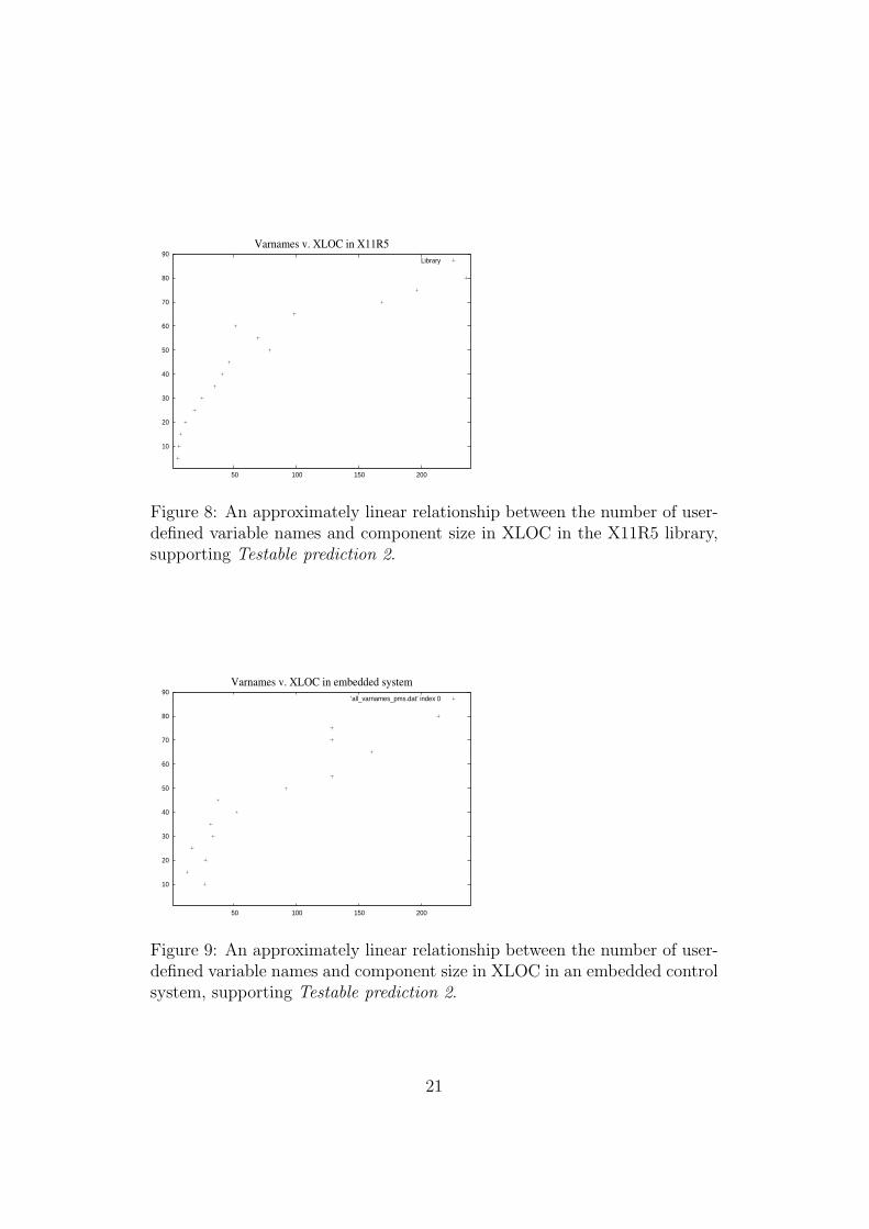
the case of C systems, it is a little less clear how to define variable namesand components as in C, the file and the function both act as interfaces indifferent ways, (functions in the standard way, but files through file scopewhen several functions share the same file as is often the case in the systemsstudied here). Even so, approximate linearity for files is again found as shownin Figures 8 (the X11R5 library) and 9 (an embedded control system). Thesame is true of the X11R5 server, although this is not shown.

No attempt will be made here to assess the statistical significance of theseas they follow by making an empirical observation about the distribution oftokens and XLOC on the back of the central result of equation (19). It ismerely suggestive of a general trend.

5 Unification with defect models and cluster-

ing

In a previous paper, [10], defect growth of xlogx where x is the number ofXLOC, was shown to be intimately related with power-law component sizedistributions in very disparate systems. There is another very interestingempirically observed property of defects in software systems; they cluster. Forexample, the effect is sufficiently pronounced that [2] include it as propertynumber four in a defect top ten list and quote several sources noting that

20

10

20

30

40

50

60

70

80

90

50 100 150 200

Varnames v. XLOC in X11R5

Library

Figure 8: An approximately linear relationship between the number of user-defined variable names and component size in XLOC in the X11R5 library,supporting Testable prediction 2.

10

20

30

40

50

60

70

80

90

50 100 150 200

Varnames v. XLOC in embedded system

’all_varnames_pms.dat’ index 0

Figure 9: An approximately linear relationship between the number of user-defined variable names and component size in XLOC in an embedded controlsystem, supporting Testable prediction 2.

21

“80% of the defects appear in 20%” of the modules. This is however a well-known property of Pareto or power-law distributions.

The model presented here gives a possible explanation for this and more-over, suggests that they may actually be different facets of the same phe-nomenon. Consider equation (19). Supposing that each time a token ti isused, the assumption is made that there is some constant probability p ofmaking a mistake, i.e. creating a defect. Then, the total number of defects ina component, di = p.ti. Substituting this in equation (19) and using equation(23) again, yields

pi =(ai)

−β

Q(β)∼ (ti)

−β ∼ (di)−β (25)

leading to,

5.0.4 Testable prediction 3:

The probability that di defects will appear in a component approximately obeysa power law or Pareto distribution if the probability of making a mistake isconstant with any token.

Quite apart from the studies reported by [2], this can be demonstratedhere on two datasets for which there is a particularly good defect record ofconsiderable maturity, that of the NAG scientific subroutine Fortran and Clibraries as shown in Tables 2 and 3, [11]. In both cases, defect clustering ismanifestly present.

Number of defects Number of components NXLOC

0 2865 (78.30%) 179947 (67.62%)1 530 (14.48%) 47669 (17.91%)2 129 (3.53%) 14963 (5.62%)3 82 (2.24%) 13220 (4.97%)4 31 (0.84%) 5084 (1.91%)5 10 (0.27%) 1195 (0.45%)6 4 (0.11%) 1153 (0.43%)7 3 (0.08%) 1025 (0.39%)8 0 (0.00%) 0 (0.00%)9 0 (0.00%) 0 (0.00%)10 4 (0.12%) 1653 (0.62%)11 1 (0.03%) 214 (0.08%)

22

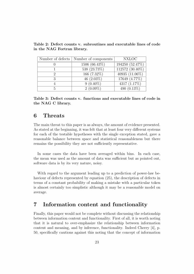
Table 2: Defect counts v. subroutines and executable lines of codein the NAG Fortran library.

Number of defects Number of components NXLOC

0 1506 (66.43%) 194250 (52.47%)1 538 (23.73%) 112572 (30.40%)2 166 (7.32%) 40935 (11.06%)3 46 (2.03%) 17649 (4.77%)4 9 (0.40%) 4317 (1.17%)5 2 (0.09%) 490 (0.13%)

Table 3: Defect counts v. functions and executable lines of code inthe NAG C library.

6 Threats

The main threat to this paper is as always, the amount of evidence presented.As stated at the beginning, it was felt that at least four very different systemsfor each of the testable hypotheses with the single exception stated, gave areasonable balance between space and statistical reasonableness but thereremains the possibility they are not sufficiently representative.

In some cases the data have been averaged within bins. In each case,the mean was used as the amount of data was sufficient but as pointed out,software data is by its very nature, noisy.

With regard to the argument leading up to a prediction of power-law be-haviour of defects represented by equation (25), the description of defects interms of a constant probability of making a mistake with a particular tokenis almost certainly too simplistic although it may be a reasonable model onaverage.

7 Information content and functionality

Finally, this paper would not be complete without discussing the relationshipbetween information content and functionality. First of all, it is worth notingthat it is natural to over-emphasize the relationship between informationcontent and meaning, and by inference, functionality. Indeed Cherry [4], p.50, specifically cautions against this noting that the concept of information

23

based on alphabets as extended by Shannon and Wiener amongst others, onlyrelates to the symbols themselves and not their meaning. Indeed, Hartley inhis original work, defined information as the successive selection of signs,rejecting all meaning as a mere subjective factor.

In other words, the development using information content from equation(6) onwards leading to the relationship expressed by equation (19) is fun-damental but it says little if anything about functionality. This stronglysuggests that power-law behaviour is nothing to do with functionality and isrelated simply to the use of alphabets of tokens to build texts such as pro-gramming systems. In other words, it operates at an even lower level thanfunctionality or meaning.

The proper study of meaning is known as semiotics. In this discipline,rules acting on signs or tokens are split into three categories:-

• Syntactic rules (rules of syntax; relations between signs)

• Semantic rules (relations between signs and the things, actions, rela-tionships and qualities known collectively as designata)

• Pragmatic rules (relations between signs and their users)

The development described here relates only to the first category.

Interestingly however, the existence of power-law behaviour in defect dis-tributions suggests that defects may have more in common with errors in theuse of the tokens of a language in the simple manner described earlier, thanin their meaning.

8 Conclusions

The paper presents four contributions each supported by real systems dataof different provenance and programming language.

• Power-law component size behaviour appears to be persistent through-out the development life-cycle. In the systems analysed, no essentialchanges were noted over long release life-cycles. This is predicted bythe next contribution.

24

• Using variational principles suggested in [10] merged with argumentsfrom Hartley-Shannon information theory, it is predicted that the prob-ability pi of a component appearing with ti tokens in any softwaresystem, whatever its implementation details, obeys a power-law withrespect to the size of its distinct alphabet of tokens ai,

pi ∼ (ai)−β (26)

• Using the simple law of equation (26) and the observation that thenumber of tokens per XLOC is approximately constant, it is furtherpredicted that the number of user-defined variable names must be ap-proximately linear with component size in XLOC.

• Also using equation (26) along with the simple assumption that thereis a constant probability of making a mistake on any token, it is alsopredicted that defects will cluster as a power-law distribution leadingdirectly to the widely-observed Pareto or 80:20 rule.

In addition, it provides a unified model with [10], whereby during the devel-opment phase, subject to constraints on the total information content and thetotal size, a power-law distribution in the alphabet used to construct eachcomponent will emerge. This in turn implies the approximate power-lawbehaviour of component size with respect to XLOC observed in [10].

When such a system is released, subject to the constraints that size and to-tal number of defects is fixed, those defects will then appear roughly as xlogxwhere x is the number of XLOC and that this phenomenon also manifestsitself as clustering.

Finally, it is hypothesized that,

• The equilibriation process which takes place leading to equation (19)takes place in the programmers’ minds as functionality is graduallytranslated into code.

• Power-law behaviour is more fundamental than functionality and ap-pears to be related only to the alphabet of tokens used.

• Defect is intimately related to information content. This can be seenhere in the close relationship between the variational principle used herein the development phase in which the externally specified variationalconstraint εi = ( Ii

ti) and that used by [10] in the release phase where

25

εi = ( di

ni), recalling that ti the number of tokens and ni, the number of

XLOC, differ on average only by a scale factor as described earlier. di

is the number of defects in component i. This may indicate that defectis more closely related to the use of the tokens themselves rather thanthe meaning of the tokens.

These hypotheses will be examined in a follow-up work as space prohibits amore detailed discussion here.

References

[1] G. Baxter, M. Frean, J. Noble, M. Rickerby, H. Smith, M. Visser,H. Melton, and E. Tempero. Understanding the shape of java software.OOPSLA ’06, 2006. http://doi.acm.org/10.1145/1167473.1167507.

[2] B. Boehm and V.R. Basili. Software defect reduction top 10 list. IEEEComputer, 34(1):135–137, 2001.

[3] D. Challet and A. Lombardoni. Bug propagation and debugging inasymmetric software structures. Physical Review E, 70(046109), 2004.

[4] Colin Cherry. On Human Communication. John Wiley Science Editions,1963. Library of Congress 56-9820.

[5] D. Clark and C. Green. An empirical study of list structures in lisp.Communications of the ACM, 20(2):78–87, 1977.

[6] G. Concas, M. Marchesi, S. Pinna, and N.Serra. Power-laws in alarge object-oriented software system. IEEE Trans. Software Eng.,33(10):687–708, 2007.

[7] A.A. Gorshenev and Yu. M. Pis’mak. Punctuated equilibrium in soft-ware evolution. Physical Review E, 70:067103–1,4, 2004.

[8] R.V.L. Hartley. Transmission of information. Bell System Tech. Journal,7:535, 1928.

[9] L. Hatton. Testing the value of checklists in code inspections. IEEESoftware, 25(4):82–88, 2008.

[10] L. Hatton. Power-law distributions of component sizes in gen-eral software systems. IEEE Transactions on Software Engineering,July/August 2009.

26

[11] T.R. Hopkins and L. Hatton. Defect correlations in a major numer-ical library. Submitted for publication, 2008. Preprint available athttp://www.leshatton.org/NAG01 01-08.html.

[12] B.W. Kernighan and R. Pike. The Unix programming environment.Prentice-Hall software series, 1984. ISBN 0-13-937681-X.

[13] Barbara Kitchenham. Counterpoint: The problem with function points.IEEE Software, 14(2):29,31, 1997.

[14] Barbara Kitchenham, Shari Lawrence Pfleeger, Beth McColl, andSuzanne Eagan. An empirical study of maintenance and developmentestimation accuracy. J. Syst. Softw., 64(1):57–77, 2002.

[15] J.C. Knight and N.G. Leveson. An experimental evaluation of the as-sumption of independence in multi-version programming. IEEE Trans-actions on Software Engineering, 12(1):96–109, 1986.

[16] G.A. Miller. Some effects of intermittent silence. American Journal ofPsychology, 70:311–314, 1957.

[17] Michael Mitzenmacher. Dynamic models for file sizes and double paretodistributions. Internet Mathematics, 1(3):305–333, 2003.

[18] Christopher R. Myers. Software systems as complex networks: Struc-ture, function and evolvability of software collaboration graphs. PhysicalReview E, 68(046116), 2003.

[19] M. E. J. Newman. Power laws, pareto distributions and zipf’s law.Contemporary Physics, 46:323–351, 2006.

[20] A. Potanin, J. Noble, M. Frean, and R. Biddle. Scale-free geometry inOO programs. Comm. ACM., 48(5):99–103, May 2005.

[21] P.K. Rawlings, D. Reguera, and H. Reiss. Entropic basis of the paretolaw. Physica A, 343:643–652, July 2004.

[22] C.E. Shannon. A mathematical theory of communication. Bell systemtechnical journal, 27:379,423, July 1948.

[23] M.L. Shooman. Software Engineering. McGraw-Hill, 2nd edition, 1985.

[24] D.F. Swayne, D. Cook, and A. Buja. Xgobi: A system for multivariateanalysis, 1998. http://www2.research.att.com/areas/stat/xgobi/ andhttp://www.ggobi.org/, accessed 12-Dec-2009.

27

[25] Meine J.P. van der Meulen. The effectiveness of software diversity. Ph.D.Thesis, City University, London, 2008.

28