Columbia University, Electrical EngineeringTechnical Report #2011-05-06, Nov. 2011

Power Grid Vulnerability to GeographicallyCorrelated Failures –

Analysis and Control ImplicationsAndrey Bernstein∗†, Daniel Bienstock‡, David Hay§, Meric Uzunoglu∗, and Gil Zussman∗

∗Department of Electrical Engineering, Columbia University, New York, NY 10027†Department of Electrical Engineering, Technion, Haifa 32000, Israel,

‡Department of Applied Physics and Applied Math, Columbia University, New York, NY 10027§School of Engineering and Computer Science, Hebrew University, Jerusalem 91904, Israel

Email: andreyb@techunix.technion.ac.il, dano@columbia.edu, dhay@cs.huji.ac.il,meric.uzunoglu@gmail.com, gil@ee.columbia.edu

Abstract—We consider power line outages in the transmissionsystem of the power grid, and specifically those caused bya natural disaster or a large scale physical attack. In thetransmission system, an outage of a line may lead to overloadon other lines, thereby eventually leading to their outage. Whilesuch cascading failures have been studied before, our focus ison cascading failures that follow an outage of several lines inthe same geographical area. We provide an analytical modelof such failures, investigate the model’s properties, and showthat it differs from other models used to analyze cascades inthe power grid (e.g., epidemic/percolation-based models). Wethen show how to identify the most vulnerable locations in thegrid and perform extensive numerical experiments with real griddata to investigate the various effects of geographically correlatedoutages and the resulting cascades. These results allow us togain insights into the relationships between various parametersand performance metrics, such as the size of the original event,the final number of connected components, and the fraction ofdemand (load) satisfied after the cascade. In particular, we focuson the timing and nature of optimal control actions used to reducethe impact of a cascade, in real time. We also compare resultsobtained by our model to the results of a real cascade thatoccurred during a major blackout in the San Diego area onSept. 2011. The analysis and results presented in this paperwill have implications both on the design of new power gridsand on identifying the locations for shielding, strengthening, andmonitoring efforts in grid upgrades.

Index Terms—Power Grid, Geographically-Correlated Fail-ures, Cascading Failures, Resilience, Survivability.

I. INTRODUCTION

Recent colossal failures of the power grid (such as theAug. 2003 blackout in the Northeastern United States andCanada [2], [37]) demonstrated that large-scale and/or long-term failures will have devastating effects on almost every as-pect in modern life, as well as on interdependent systems (e.g.,telecommunications, gas and water supply, and transportation).Therefore, there is a need the study the vulnerability of theexisting power transmission system and to identify ways tomitigate large-scale blackouts.

The power grid is vulnerable to natural disasters, such asearthquakes, hurricanes, floods, and solar flares [38] as well as

Fig. 1. The graph that represents part of the Western Interconnect andsections of the Texas, Oklahoma, Kansas, Nebraska, and the Dakotas’ grids.Green dots are demands (loads), red dots are supplies (generators), and neutralnodes are not shown. This graph was used to derive numerical results.

to physical attacks, such as an Electromagnetic Pulse (EMP)attack [17], [18], [38]. Thus, we focus the vulnerability of thepower grid to an outage of several lines in the same geograph-ical area (i.e., to geographically-correlated failures). Recentworks focused on identifying a few vulnerable lines throughoutthe entire network [7], [8], [32], on designing line or nodeinterdiction strategies [9], [34], and on characterizing thenetwork graph and studying probabilistic failure propagationmodels [12], [16], [23], [25], [39], [41]. However, our objec-tive is to identify the most vulnerable areas in the power grid,and examine appropriate real-time control countermeasures tominimize the impact of an event of this type. Detection of themost vulnerable areas has various practical applications, sincethe system in these areas can be either shielded (e.g., againstEMP attacks or solar flares), strengthened (e.g., by increasingthe capacities of some relevant lines), or monitored (e.g., aspart of smart grid upgrade projects). Real-time control willlikely still be needed, in case the pre-strengthening of the gridhas overlooked a particular “attack” pattern.

Unlike graph-theoretical network flows, the flow in the

power grid is governed by the laws of physics and there areno strict capacity bounds on the lines [6], [16], [27]. Onthe other hand, there is a rating threshold associated witheach line, such that when the flow through a line exceedsthe threshold, the line heats up and eventually faults. Suchan outage, in turn, causes another change in the power grid,that can eventually lead to a cascading failure. We describethe linearized (i.e., DC) power flow model and the cascadingfailure model (originated from [13] and extended in [7], [8])that allow us to obtain analytic and numerical results despitethe problem’s complexity. We note that severe cascadingfailures are hard to control in real time [4], [7], [8], [16],[31], since the power grid optimization and control problemsare of enormous size. Thus, in our numerical experiments, weapply basic control mechanisms that shed demands at the endof each round.

We initially use the linearized power flow model to studysome simple motivating examples and to derive analyticalresults regarding the cascade propagation in simple ring-basedtopologies. We note that several previous works (e.g., [12],[25], [30], [35], [41] and references therein) assumed that aline or node failure leads with some probability to a failureof nearby nodes or lines. Such epidemic-based modelingallows using percolation-based tools to analyze the effects ofa cascade. However, we show that using the more realisticpower flow model leads to failure propagation characteristicsthat are significantly different. Specifically, we show thata failure of a line can lead to a failure of a line M hopsaway (with M arbitrarily large). This result is of particularimportance, since it has been observed in real cascades (as therecent one in the San Diego area, discussed in Section VIII).Moreover, we prove that cascading failures can last arbitrarilylong time and that a network whose topology is a subgraphof another topology can be more resilient to failures.

In this paper, we focus on contingency events in a gridthat are initiated by geographically correlated failures. Werepresent the area affected by a contingency by a disk. Sincesuch a disk can theoretically be placed in an infinite numberof locations, we briefly discuss an efficient computationalgeometric method (which builds on results from [1]) thatallows identifying a finite set of locations that includes allpossible failure events.

In our numerical experiments, we use the WECC (Western-Interconnect) real power grid data taken from the Platts Ge-ographic Information System (GIS) [33] (the resulting graphappears in Figure 1). We present extensive numerical resultsobtained by simulating the cascading failures for each ofthe possible disk centers (the results have been obtainedby repeatedly and efficiently solving very large systems ofequations). When only few lines initially fault, cascadingfailures usually start slowly and intensify over time [7], [8].However, when the failures are geographically correlated, wenotice that in many cases this slow start phenomenon doesnot exist. We illustrate the effects of the most (and the least)devastating failures and show the yield (the overall reductionin power generation) for all different failure locations in the

Western US. Moreover, we identify various relations betweenparameters and performance metrics (such as yield, number ofcomponents into which the network partitions, and number offaulted lines which corresponds to the length of the repairprocess). We also study the sensitivity of the results todifferent failure models (stochastic vs. deterministic model),to the value of the Factor of Safety (the ratio between linecapacity and normal flow on the line), and to whether or notthe line capacities are derived based on N − 1 contingencyplan.

While large scale cascades are quite rare [13], during ourwork on this report, a cascade took place in the San Diegoarea (on Sept. 8, 2011). The causes of this cascade arestill under investigation. Yet, we have been able to use somepreliminary information [11] to assess the accuracy of ourmethod and parameters. We conclude by discussing some ofthe numerical results that we obtained for a similar scenarioand demonstrating that our methods have the potential toidentify vulnerable parts of the network.

Finally, we consider optimal control actions to be takenin the event of such a failure. We show, experimentally,that appropriate action taken at the appropriate time (and notnecessarily at the start of the cascade) can rapidly stop theprocess, while losing a minimum quantity of demand.

Below are the main contributions of this paper. First, weobtain analytical results regarding network vulnerability andresilience under the power flow model which is significantlydifferent from the classical network flow models. These resultsprovide insights that significantly differ from insights obtainedfrom epidemic/percolation-based models. Second, we combinetechniques from optimization, computational geometry, andcommunications network vulnerability analysis to developa method that allows obtaining extensive numerical resultsregarding the effects of geographically correlated failures on areal grid. To the best of our knowledge, this is the first attemptto obtain such results using real geographical data. Third,we briefly illustrate that control actions have the potential tomitigate the effects of even the worst case failure. The resultsobtained in this paper will provide insight into the design ofcontrol algorithms and network architectures.

The rest of the paper is organized as follows. In Section IIwe present the related work and in Section III we describe thepower flow and cascade models. Section IV provides analyt-ical results regarding simple network topologies. Section Vpresents the method used to set some of the parameters andthe algorithm used to identify the most vulnerable locationswithin the grid. Section VI describes the power grid dataused in this paper . In Section VII we present our numericalfindings regarding large scale failure and in Section VIII wediscuss the recent cascade in the San Diego area. SectionIX describes optimal control methods and their impact in theparticular case of one of the simulated worst-case events thatwe compute. Section X provides concluding remarks anddirections for future work.

2

II. RELATED WORK

The power grid and its robustness have drawn a lot ofattention recently, as efforts are being made to create a smarter,more efficient, and more sustainable power grid (see, e.g., [2],[19]). The power grid is traditionally modeled as a complexsystem, made up of many components, whose interactions(e.g., power flows and control mechanisms) are not effectivelycomputable (e.g., [3], [6] and references therein).

When investigating the robustness of the power grid, cas-cading failures are a major concern [2], [13], [16], [22]. Thisphenomenon, along with other vulnerabilities of the powergrid, was studied from a few different viewpoints. First, sev-eral papers studied common topological properties of powergrid networks and probabilistic failure propagation models,so that one can evaluate the behavior of a generic grid as aself-organized critical system using, for example, percolationtheory (see [5], [12], [23], [25], [26], [30], [35], [39], [41] andreferences therein). These works are closely related to a longline of research in the power community which uses montecarlo techniques to analyze system reliability (e.g., [10])

Another major line of research focused on specific (mi-croscopic) power flow models and used them to identify afew vulnerable lines throughout the entire network [7], [8],[32]. In particular, [9], [34] focus on designing line or nodeinterdiction strategies that will lead to an effective attack on thegrid. Since the problem is computationally intractable, mostof these papers use a linearized direct-current (DC) model,which is a tractable relaxation of the exact alternating-current(AC) power flow model. In addition, the initial failure events(causing eventually the cascading failures) are assumed tobe sporadic link outages (and in most cases, a single linkoutage), with no correlation between them. On the contrary,we focus on events that cause a large number of failures in aspecific geographical region (e.g., [18], [38]). To the best ofour knowledge, geographically-correlated failures in the powergrid have not been considered before and have been studiedonly recently in the context of communication networks [1],[14], [21], [29], [36].

Moreover, since cascading failures are highly dependenton the network topology, we use the real topology of thewestern U.S. power grid. While building on the linearizedmodel, we manage to obtain numerical results for a verylarge scale real network (results for large networks have beenderived in the past using mostly probabilistic models [12],[23], [30]). Perhaps, closest to us in its approach is [31]that analyzes the effects of single line failures on the Polishpower grid. Yet, while [31] considers a real topology, itdoes not take into account geographical effects. Moreover,it applies control mechanisms that are more sophisticatedthan the ones considered here. Control mechanisms are alsointroduced in [4] that develops a method to trade off loadshedding and cascade propagation risk. Recently, [27], [28]proposed efficient optimization algorithms for solving theclassical power flow problems. These algorithms use efficientmathematical programming methods and can support offline

control decisions. However, they are not applicable when rapidonline control of the grid is required.

III. BASIC MODELS

We adopt the linearized (or DC) power flow model, whichis widely used as an approximation for more realistic non-linear AC power model (see [6] for a survey on the powerflow models). In particular, we follow [7], [8] and representthe power grid by a directed graph G, whose set of nodesis N . Each of these nodes is classified either as a supplynode (“generator”), a demand node (“load”), or a neutral node.Let D ⊆ N be the set of the demand nodes, and for eachnode i ∈ D, let Di be its demand. Also, C ⊆ N denotesthe set of the supply nodes and for each node i ∈ C, Pi isthe active power generated at i. The edges of the graph Grepresent the transmission lines. The orientation of the linesis arbitrarily and is simply used for notational convenience.We also assume pure reactive lines, implying that each line(i, j) is characterized by its reactance xij .

Given supply and demand vectors (P,D), a power flow isa solution (f, θ) of the following system of equations:

∑(i,j)∈δ+(i)

fij −∑

(j,i)∈δ−(i)

fji =

Pi, i ∈ C−Di, i ∈ D0, otherwise

(1)

θi − θj − xijfij = 0, ∀(i, j) (2)

where δ+(i) (δ−(i)) is the set of lines oriented out of (into)node i, fij is the (real) power flow along line (i, j), and θi isthe phase angle of node i. These equations guarantee powerflow conservation in each neutral node, and take into accountthe reactance and power capacity of each line. In addition,since the orientation of lines is arbitrary, a negative flow valuesimply means a flow in the opposite direction.

When G is fully connected and∑

i∈C Pi =∑

i∈D Di, (1)–(2) has a unique solution [8, Lemma 1.1]. This holds evenwhen G is not connected but the total supply and demandwithin each of the connected components are equal.

We note that the DC power flow model resembles anelectrical circuit model, where phase angles are analogous tovoltages, reactance is analogous to resistance, and the powerflow is analogous to the current. The following observation,which is analogous to Kirchoff’s law, captures the essenceof the model and provides easier way to look at (1)–(2)analytically. It uses the notion of a path between nodes, whichis an alternating sequence of lines and adjacents nodes. (Proofis in the appendix).

Observation 3.1: Consider two nodes a and b and twopaths π1 = (a, e0, v0, e1, v1, . . . , b) and π2 = (a, e′0, v

′0, e

′1, v

′1,

. . . , b). The sum of the flow-reactance product feixei alongthe lines of path π1 is equal to the sum of the flow-reactanceproduct along the lines of path π2. Specifically, the flowsalong parallel lines with the same reactance is the same.

Next we describe the Cascading Failure Model. We assumethat each line (i, j) has a predetermined power capacity uij ,which bounds its power flow in a normal operation of the

3

Cascading Failure Model (Deterministic Case)

Input: Connected network graph G.Initialization: Before time step t = 0, we have that

∑i∈C Pi =∑

i∈D Di (i.e., the power is balanced), (1)–(2) are satisfied for G, andall flows along all lines are within the corresponding power capacity.Failure event: At time step t = 0, a failure of some subset of linksof G occurs. Let G.changed = true.While G.changed is true do:

1) Adjust the total demand to the total supply within eachcomponent of G.

2) Use the system (1)–(2) to recalculate the power flow in G.3) For all lines compute a moving average

f tij = α|fij |+ (1− α)f t−1

ij

4) Remove from G all lines with flow moving average abovepower capacity (f t

ij > uij). If at least one line was removedat this step, let G.changed = true; otherwise, let G.changed =false.

system (that is, |fij | ≤ uij). We assume that before a failureevent, G is fully connected, the total supply and demand areequal, the power flows satisfy (1)–(2), and the power flowof each line is at most its power capacity. Upon a failure,some lines are removed from the graph, implying that itmay become disconnected. Thus, within each component,we adjust the total demand to equal the total supply, bydecreasing the demand (supply) by the same factor at allloads (generators). This process is sometimes called demandshedding and naturally it causes a decrease in demand/supply.Then, we use (1)–(2) to recalculate the power flows in the newgraph. The new flows may exceed the capacity and as a result,the corresponding lines will become overheated. Thermaleffects cause overloaded lines to become more sensitive toa large number of effects each of which could cause failure.We model outages using a moving average of the power flow,using a value f t

ij = α|fij | + (1 − α)f t−1ij (in this paper, we

mostly use either α = 0.5 or α = 1). To first order, thisapproximates thermal effects, including heating and coolingfrom prior states. A similar moving average model wasconsidered in [4], [8]. A general outage rule gives the faultprobability of line (i, j), given its moving average f t

ij . In thispaper, we consider the following rule:

P {Line (i, j) faults at round t} =

1, f t

ij > (1 + ε)uij

0, f tij ≤ (1− ε)uij

p, otherwise.(3)

where 0 ≤ ε < 1 and 0 ≤ p ≤ 1 are parameters. Whenε = 0, we obtain a deterministic version of this rule. In thiscase, lines (i, j) whose f t

ij is above the power capacity uij

are removed from the graph.The process is repeated in rounds until the system reaches

stability, namely until there is an iteration in which no linesare removed. We note that our model does not have a notionof exact time, however the relation between the elapsed timeand the corresponding time can be adjusted by using different

2

2

2

1

1

11

1

1

Area M − 1Area 0

Area 1

tie line

tie line

0.5

0.5

0.5

0.5

Fig. 2. The M -ring RM . Each generation node and its two adjacent demandnode are a self-sustained area. No power flow is transmitted between theseareas (that is, along the tie lines).

values of α; in a sense, up to a certain degree, smaller value ofα implies that we take a more microscopic look at the cascade.

Our major metric to assess the severity of a cascading failureis the system post-failure yield which is defined as follows:

Y , The actual demand at the stabilityThe original demand

. (4)

In addition to the yield, other performance metrics will beconsidered, such as the number of faulted lines, the numberof connected components, and the maximum line overload.While the yield naturally gives an assessment of the severityof the cascade after the process has already finished, the othermetrics may also shed light on the cascade properties after afixed (given) number of rounds.

Note that our model contains a very simple control mech-anism, namely, round-by-round demand shedding. In Sec-tion IX, we consider more elaborated control mechanisms andcompare the results.

IV. CASCADING FAILURES PROPERTIES IN SIMPLEGRAPHS

In this section we describe important properties of thepower flow and cascading failure models in a simple graph.Specifically, we show that unlike other flow models, cascadingfailures in a power flow network are harder to predict and aredifferent from epidemic-like failure models, from the followingfour reasons:

1) Consecutive failures in a cascade may happen within anarbitrarily long distance of each other.

2) Cascading failures can last arbitrarily long time.3) A network G1 whose topology is a subgraph of another

network G2 can be more resilient to failures than G2.4) A failure event which results in initial failure of some

set of lines A can cause more damage than a failureevent, whose initial set of faulted lines is a superset ofA.

In order to prove the results, we use the following simplepower flow topology, which is depicted in Figure 2

Definition 1: An M -ring RM = ⟨C ∪ D, E⟩ is a directedgraph with M supply nodes C = {0, . . . ,M−1}, 2M demand

4

nodes D = {M, . . . , 3M − 1}, two parallel transmission linesconnecting each generator i ∈ C to demand node M + 2i,two parallel transmission lines connecting generator i ∈ Cto demand node M + 2i + 1, and a single transmission lineconnecting demand node M +2i+1 (i ∈ C) to demand nodeM+(2i+2 mod 2M)1. For each i ∈ C, the generation valueis Pi = 2, and the demand values are D2i = D2i+1 = 1. Thereactance value xij of all transmission lines is 1.

Clearly, one can view the M -ring as a collection of Mself sustained areas: each generator i supplies the demandsof M + 2i and M + 2i + 1. For brevity, we call the linesconnecting i and M+2i even lines, the lines connecting M+2i+ 1 odd lines, and the lines connecting two demands (thatis, connecting two self-sustained areas) tie lines. Moreover,we refer to odd and even lines collectively as internal lines.

By symmetry, we have the same power flow on all evenlines and odd lines. The solution of (1)–(2) verifies that thisis indeed the case: a power flow of 0.5 is transmitted fromeach generator along its 4 adjacent internal lines, as shown inFigure 2, the phase angle of all generators is the same, andthe phase angle of all demand nodes is the same. This alsoimplies that there is no flow on the tie lines. Notice that ifall lines has a power capacity of 0.5, it suffices to sustain thatpower flow.

In the rest of the section, we will consider the followingtypes of failure events:

• Area failure: The four internal lines within Area i,as well as the two lines connecting Area i to the ad-jacent areas, fault. Namely, lines (i,M + 2i), (i,M +2i)′, (i,M + 2i + 1), (i,M + 2i + 1)′, (M + (2i − 1mod 2M),M+2i), (M+2i+1,M+(2i+2 mod 2M))fault.

• Parallel lines failure: Two parallel internal lines withinArea i fault. Without loss of generality, we consider onlyeven parallel lines, that is, (i,M + 2i) and (i,M + 2i)′

fault.• Odd line and even line failure: One odd line and one

even line within Area i fault. Namely, lines (i,M + 2i)and (i,M + 2i+ 1) fault.

• Single internal line failure: Single internal line in Area ifaults. Without loss of generality, we consider only evenline, that is, line (i,M + 2i) faults.

• Tie line and internal line failure: Internal line in Area i,as well as the tie line connected to the correspondingdemand, fault. Without loss of generality, we consideronly an even line and its corresponding tie line, that is,(i,M +2i) and (M +(2i− 1 mod 2M),M +2i) fault.

It is important to notice that these failures cover the possibletypes of geographical failures over the ring (some combina-tions of these failures can also occur if the failure radius islarge enough). In this section, we will not consider sporadicfailure events (that is, in which the outaged lines are notgeographically-correlated), or initial events that partition the

1Parallel transmission lines are denoted (i, j) and (i, j)′. The orientationof the lines is only for notational convenience.

graph such that there is a component whose total demand isnot equal to its total generation.

We next compare between an area failure and parallel linesfailure. As for area failure, it is easy to see that the samepower flow solution still holds, and therefore, the power flowalong all operating lines does not change. The loss of demandis only 2 units and the resulting yield is M−1

M . On the otherhand, upon parallel lines failure, the entire generation of nodei must be transmitted on the only operating lines connected tonode i: (i,M+2i+1) and (i,M+2i+1)′. Since the lines areparallel, by symmetry, each of these lines transmits a powerof 1 unit (cf. Observation 3.1). In addition, by (1), the tie lineconnecting area i to area i + 1 carries power of 1 unit sincenode 2i+1’s demand is only 1. Now focus on Area i+1. Thetotal amount of incoming generation to this area is 3 units (2units generated in node i+1 and one along the tie line in Areai), while the total demand is 2 units. This immediately impliesthat the tie line to Area i+2 carries one unit of power. As forthe flows on the lines within that area, one can verify that avalid (and therefore the only) solution of (1)–(2) has no powerflow on lines (i + 1,M + 2i + 2) and (i + 1,M + 2i + 2)′

and one unit of power flow along (i + 1,M + 2i + 3) and(i+ 1,M + 2i+ 3)′. This flow assignment is identical to theassignment of Area i, and therefore, by inductive arguments, itis valid for all the areas in the ring. Moreover, there are threephase values in the solution: one for all generation nodes, onefor all even demand nodes, and one for all odd demand nodes.

Based on the power capacity of the lines uij , the movingaverage parameter α of the cascading failure model, and theFoS of the entire system, we can derive the following results(all proofs are in the appendix):

Lemma 4.1: Consecutive failures in a cascade may happenwithin an arbitrarily long distance of each other.

We note that Lemma 4.1 captures an important differencebetween our model and previously-suggested models, thatassume that power grid failures propagate in an epidemic-like manner. While, under these models, a line failure causesonly adjacent node/line (or a line with small distance) to fault,our model captures situations in which the cascade “skips”’large distances within a single iteration. As we will discussin Section VIII, this was indeed the case in a recent real-lifecascade causing a major blackout in California.

Lemma 4.2: A failure of o(1) of the lines may cause anoutage of a constant fraction of the lines, within one iteration.

The following two lemmas show that the failures do notalways behave monotonically:

Lemma 4.3: An initial failure event of some set of lines Amay result in a lower yield than a failure event, whose initialset of faulted lines is a superset of A.

Lemma 4.4: A network G1, whose topology is a subgraphof the topology of another network G2, may obtain higheryield.

We note that in practice, if the failures are geographicallycorrelated, non-monotone situations, as described in Lem-mas 4.3 and 4.4, rarely happen. Thus, in the rest of the paper(and specifically, in the algorithm described in Section V-B),

5

we assume only a monotone behavior of the failures.Up until now, we dealt with very specific type of failures,

which intuitively breaks the ring into a chain. In general, suchfailures are easier to analyze since (2) does not form contraintsin a cyclic manner (that is, one can assign the phase value ofthe nodes based only on the flows and the phase value of thenodes that precedes it). More formally, this extra difficultyis captured by Observation 3.1, and looking at the differentpaths between each pair of nodes. When the ring breaks intoa chain, all these paths follow one “direction”. On the otherhand, when the ring does not break, there are both clockwiseand counter-clockwise paths that need to be considered. Wedemonstrate this difference by comparing a single internal linefailure of line (0,M) (that does not break the ring into chain)with a tie line and internal line failure of lines (0,M) and(3M − 1,M) (which breaks the ring into chain).

In the tie line and internal line failure, one can simply assigna power flow of 1 unit along the parallel line (0,M)′, wherethe phase difference between node 0 and M is 1 (to meetthe constraint of (2)); the rest of the flows and phases remainunchanged. However, this solution is not valid in case of asingle internal line failure, since there is a phase differencebetween node M and 3M − 1, and therefore, it is impossiblethat no flow traverses the operating line between them. Wenote also that in the odd and even lines failure (which doesnot break the chain either), the flows on the lines parallel to thefailures increase to 1 by changing solely the generator phase.Since the demand nodes’ phases do not change, this failure islocalized within that single area.

We next show that the power flow values induced by thesingle line failure change across the entire graph and dependson the value of M :

Lemma 4.5: Consider an M -ring, in which line (0,M)failed. Then, after the first iteration:(i) The flow along line (0,M)′ is 2M/(2M + 0.5).(ii) The flow along all other even lines is M/(2M + 0.5).(iii) The flow along all odd lines is 1−M/(2M + 0.5).(iv) The flow along all tie lines is 1− 2M/(2M + 0.5).

Corollary 4.6: An M -ring requires power capacity of 1/9on its tie lines and a power capacity of 1 on its internal linesto withstand any failure of one line.

Interestingly, one can see that as M gets larger, a singleinternal line failure has the same effect as the correspondingtie line and internal line failure. This stems from the factthat the closed-loop effects, initially distinguishing betweenthe failures, are fading away as the ring gets larger.

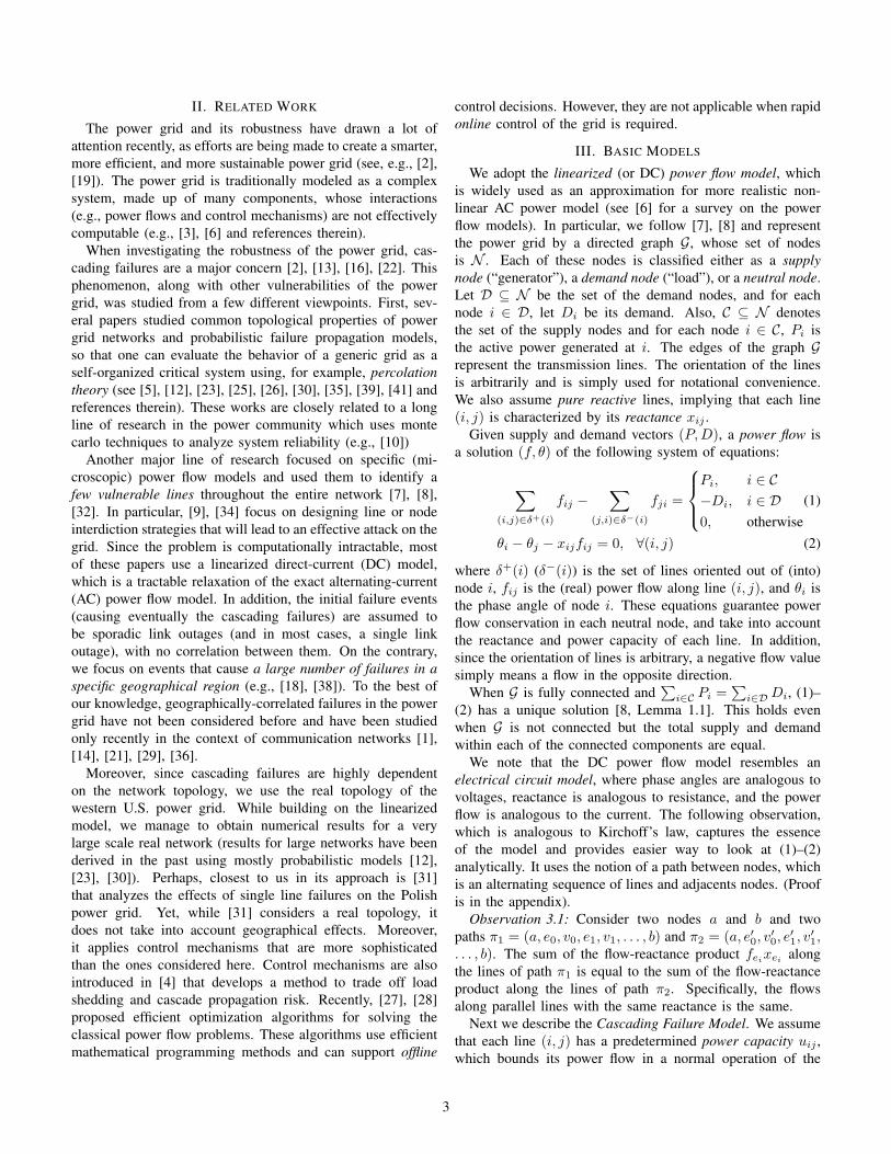
Finally, the next lemma shows that, unlike the examples wepresented on the ring, cascades can be made arbitrarily long(in time). The lemma uses another topology which is depictedin Figure 15.

Lemma 4.7: The length of the cascade (the number ofiterations until the system stabilizes) can be arbitrarily large.

To conclude, using simple examples we highlight the diffi-culties and differences between prior models used to analyzethe power grid and the models we use. In the rest of the paper,we will investigate how these models behave in real-life power

grid and geographically-correlated failures.

V. POWER GRID RESILIENCE

A. Parameters Set-up

We note that in the cascading failure model, the powercapacities uij of the lines are given a-priori. In practice,however, these capacities are hard to obtain and are usuallyestimated based on the actual operation of the power grid. Inthis paper, we take the N−k contingency analysis approach [8]in order to estimate the power capacities. Namely, we setthe capacities so that the network is resilient to failure ofany set of k out of the N lines. In addition, we considerover-provisioning of lines capacity by a constant fraction ofthe required capacity of each line. This over-provisioningparameter, denoted by K, is often referred to as the Factor ofSafety (FoS) of the grid.

Specifically, we focus on the following two cases.• N -resilient grids (that is, k = 0). In this case, we solve

(1)–(2) for the original grid graph (without failures) andset the power capacity to uij = K · fij , where K ≥ 1.

• (N − 1)-resilient grids (that is, k = 1). In this case,we solve (1)– (2) for N graphs, each resulting from asingle line failure event. The power capacity is set touij = K · maxr f

rij , where fr

ij is the flow assigned toline (i, j) when considering the rth failure event.

It is worth mentioning that the real power grid is usuallyassumed to be at least N -resilient with K ≈ 1.2 [15]. Onthe other hand, some data show that certain lines (or, moregenerally, paths) are more resilient than others. For example,a historical transmission paths data found in [40] shows thatsome transmission paths have power capacities which are 1.1times their normal flow, while others have an FoS larger than2. Nevertheless, the average FoS is indeed around 1.2. Inaddition, utility companies usually guarantee that their grid isat least (N−1)-resilient [8]2. Therefore, by setting the powercapacities parameters, we examine in this paper both N - and(N−1)-resilient grids with different FoS values K. Most ofour numerical results are presented for a grid with FoS K =1.2.

B. Identification of Vulnerable Locations

We consider a circular and deterministic failure model,where all lines and nodes within a radius r of the failure’sepicenter are removed from the graph (this includes linesthat pass through the affected area). In addition, we assumemonotonicity of failures: if the initial set of faulted lines dueto event A is a subset of the faulted lines due to event B,then the yield of A is at least that of B. We note that in thegeneral case, this property does not hold (see Lemma 4.3).However, we observed that such events rarely happen in realpower grid systems, and when they do, it is only when bothevents have a marginal effect. Since our goal is to identify the

2We note that early reports on the recent San Diego blackout indicate thatthis was not the case.

6

most vulnerable locations in a real power grid, this is a validassumption for practical purposes.

To identify the candidates for the most vulnerable locations,we use computational geometric methods developed in [1] foridentifying the vulnerable locations in fiber-optic networks.For each line, we define an r-hippodrome, which capturesall points in the plane R2 whose distance from the line is atmost the failure radius r. We focus on the arrangement ofhippodromes, which is the subdivision of the plane into ver-tices, arcs, and faces. The vertices are the intersection pointsof the hippodromes, the arcs are either maximally connectedcircular arcs or straight line segments of the boundaries ofhippodromes that occur between the vertices, and faces aremaximally connected regions bounded by arcs.

Once the vertices of the arrangements are identified, we treateach vertex v as a candidate for a failure epicenter and denoteby L(v) the set of lines within radius r of v (L(v) can be easilyfound). We then use the Cascading Failure Model, describedin Section III, with L(v) as the set of lines that initially fault.Naturally, the process of checking all candidates (each with adifferent initial failure event) can be easily parallelized.

Arrangements are well-established concept in computationalgeometry, and it can be easily shown that in order to findthe vulnerable locations, it is sufficient to consider only thevertices of the arrangements. In particular, for any point p ∈R2, there is a vertex v such that L(p) ⊆ L(v). Notice thatcomputing arrangements is quadratic in the number of lines.Thus, we parallelized this computation as well by partitioningthe graph into several sections (with small number of lines)and finding vertices of the arrangements in each section. Toensure that no vertices are lost in the border between twosections, the sections have a 2r overlap.

VI. POWER GRID DATA

We use real power grid data of the western US takenfrom the Platts Geographic Information System (GIS) [33].This includes the information about the transmission lines,power substations, power plants, and the population at eachgeographic location. Since, in GIS each transmission line isdefined as a link between two power substation, substationsare used as nodes in our graph. In order not to expose thevulnerability of the real grid, we used a part of the WesternInterconnect system which does not include the Canada andMexico sections. On the other hand, we attached to the gridthe Texas, Oklahoma, Kansas, Nebraska, and the Dakotas’grids, which are not part of the Western Interconnect. Theresulting graph (see Figure 1) has 14,968 nodes (substations)and 19,513 lines. Moreover, it has 1,920 power stations whichwere merged with the substations as described below. We notethat there is a small number of very dense areas (e.g., the LosAngeles area), while the rest of the grid is very sparse. Thisstructure can be seen in many other typical power grids, suchas the US Eastern Interconnect as well as European systems.Furthermore, recent research on topological models for powergrid systems show similar results [23]. Thus, our results willprobably carry over to other grids.

We performed the following processing steps for this graph.Coordinate transformation: The coordinates of the substa-tions in the GIS system are given by their longitude andlatitude. We transformed these to planar (x, y) coordinates,using the great-circle distance method.Connectivity check: We identified the connected componentsof the raw GIS graph, which consists of one large connectedcomponent and few small ones. Moreover, we identified somesubstations that appear in the transmission lines data but areabsent in the substations data. The number of these substationsis small, and therefore, after manual inspection, they wereeither eliminated or merged with other nearby substations (seealso the next step).Nodes merging and lines elimination: For each node outsidethe large component, we found the closest node within thelarge component. If the distance between them was below agiven threshold (10 Km), we merged the two nodes. Then,the remaining disconnected nodes were inspected manuallyand were either eliminated or merged. At the end of thisprocess, we obtained a fully-connected graph (that is, a singleconnected component) with 13,992 nodes and 18,681 lines.Identifying demands and supplies: Demands were asso-ciated with the closest node to each populated area (i.e.,zip-code) and were set to be proportional to the populationsize (the normalization factor is computed by comparing thetotal population and total generation output of the entiregrid). Supplies were associated with closest node to eachpower plant (the generation capacity of the power plants istaken from the GIS). Then, for each node, we computed thedifference between its total corresponding supplies and totalcorresponding demands. Thus, all nodes were characterizedby a real number: positive for a supply node, negative fora demand node, and zero for a neutral node. The resultingcategorization appears in Figure 1. Overall, 1,117 nodes wereclassified as generators (supplies), 5,591 as loads (demands),and 7,284 as neutral. Most of the neutral nodes are closelyconnected to each other and to one of the non-neutral nodes,thus drawing the power/demand from them.Determining the system parameters: The GIS does notprovide the power capacities of the transmission lines, nor theirreactance. However, these parameters are needed for the powerflow and cascading failure models. The reactance of a linedepends on its physical properties (such as its material) andthere is a linear relation between its length and reactance: thelonger the line is, the larger its reactance. Thus, we assumedthat all lines have the same physical properties (other thanlength) and used the length to determine the reactance. It isimportant to notice that the flow part of the solution of (1)–(2) is scale invariant to the reactance (that is, multiplying thereactance of all lines by the same factor does not change thevalues of the flows). Thus, we simply use the length of theline as its reactance. Regarding the power capacities, we takethe approach described in Section V-A. In particular, we useN−k contingency analysis, with k ∈ {0, 1} and different FoSvalues K.

7

VII. NUMERICAL RESULTS

We identified the potential failure locations using the algo-rithm described in Section V-B implemented in MATLAB. Wepresent results for r = 50 kilometers, which is small enough tocapture realistic scenarios [18], [38], while it is large enough togenerate a cascading failure in most cases (the results for othervalues of r are omitted, due to space constraints). For r = 50,the algorithm identified 61,327 potential failure locations. Theidentification of these locations was done on an eight-coreserver in less than 24 hours.

For each failure location v, we performed the simulationof the Cascading Failure Model, presented in Section III,assuming that all lines in L(v) fail. The simulation wasperformed using a program that efficiently solves very largesystems of linear equations, using CPLEX [24] and Gurobi[20] optimization tools.

To assess the severity of a cascading failure, we use thefollowing four metrics, which are measured in the end of thecascade: The yield, as defined in (4); the total number ofoutaged lines, which indicates the time it takes to recover thegrid after the cascade: the larger the number of outaged lines,the longer is the actual time of the corresponding blackout;the number of connected components; and the number ofrounds until stability.

A. N-Resilience Experiments

The first set of experiments was performed after using theN contingency analysis to set the capacities of the network,with FoS K = 1.2 and K = 2.

First, we plot specific failures to show how they evolvedduring the first five rounds of the cascade. Figure 3 showsthree failure events for FoS K = 1.2: Two in California, bothleading to severe blackouts, and another one around the Idaho-Montana-Wyoming border, which had a less severe effect. Theround-by-round maximum overload (that is, maxij fij/uij)for these failures and K = 1.2 is shown in Table I. Thesame failures for K = 2 are shown in Figure 17 in theappendix. As expected, higher FoS usually leads to less severeblackout effect. Interestingly, the Idaho-Montana-Wyomingborder failure with FoS K = 1.2 leads to low yield (0.39),although the development of the failure is very slow—after5 rounds only few lines were faulted. However, the sameevent with K = 2 leads to near-unity yield. We note thatthis suggests that the assumption that K = 1.2 for all linesis quite pessimistic, as also can be seen from the actual data(see Section V-A for more details).

Scatter graphs for different metrics after 5 rounds and withFoS K = 1.2 are shown in Figure 4. It can be seen an increasein the initial number of faulted lines leads to an increase inthe total number of faulted lines at the end of the fifth round:if 400, 800, 1,200 lines initially faulted, at least 2,847, 3,600,4, 669 are faulted at the end, respectively. Furthermore, anincrease in the initial number of faulted lines leads also toan increase in the number of connected components: if 400,800, 1,200 lines initially faulted, the number of componentsis at least 696, 1,382, 1,973, respectively. Similar results for

0.326

(a) San Diego area failure event.

0.296

(b) San Francisco area failure event.

0.39

(c) Idaho-Montana-Wyoming border failure event.

Fig. 3. Illustration of cascading failures over 5 rounds for N -resilientgrid with FoS K = 1.2, where the initial failure locations are in the (a)Los Angeles area, (b) San Francisco area, and (c) Idaho-Montana-Wyomingborder. The final yields are 0.326, 0.296, and 0.39, respectively. The colorsrepresent the rounds in which the lines faulted.

K = 2 are shown in Figures 17 and 16 in the appendix. Theseresults clearly show that in this case the grid is much moreresilient to cascading failure.

Next, we analyze the severity of cascading failures oncestability is reached. Namely, when no more line failures occur.The results for FoS K = 1.2 are shown in Figure 5. In thiscase, the vast majority of the failures resulted in yield in the

8

Round MaximumOverload

1

2

3

4

774.821

1724.525

16.527

14.99

MaximumOverload

902.014

24.923

57.87

2124

MaximumOverload

6.665

1.193

1.836

1.229

San FranciscoSan Diego ID-MT-WY

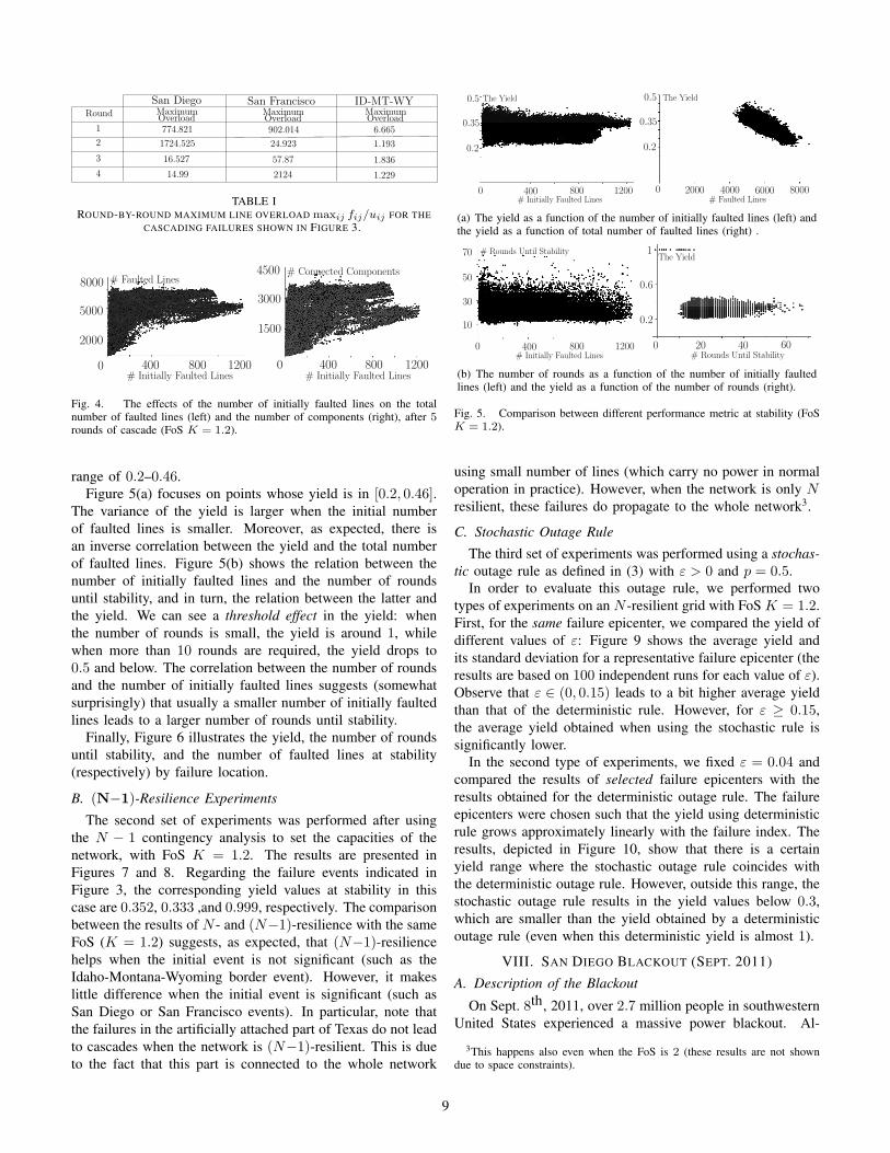
TABLE IROUND-BY-ROUND MAXIMUM LINE OVERLOAD maxij fij/uij FOR THE

CASCADING FAILURES SHOWN IN FIGURE 3.

8000

5000

2000

0 400 800 1200# Initially Faulted Lines

# Faulted Lines4500

3000

1500

0 400 800 1200# Initially Faulted Lines

# Connected Components

Fig. 4. The effects of the number of initially faulted lines on the totalnumber of faulted lines (left) and the number of components (right), after 5rounds of cascade (FoS K = 1.2).

range of 0.2–0.46.Figure 5(a) focuses on points whose yield is in [0.2, 0.46].

The variance of the yield is larger when the initial numberof faulted lines is smaller. Moreover, as expected, there isan inverse correlation between the yield and the total numberof faulted lines. Figure 5(b) shows the relation between thenumber of initially faulted lines and the number of roundsuntil stability, and in turn, the relation between the latter andthe yield. We can see a threshold effect in the yield: whenthe number of rounds is small, the yield is around 1, whilewhen more than 10 rounds are required, the yield drops to0.5 and below. The correlation between the number of roundsand the number of initially faulted lines suggests (somewhatsurprisingly) that usually a smaller number of initially faultedlines leads to a larger number of rounds until stability.

Finally, Figure 6 illustrates the yield, the number of roundsuntil stability, and the number of faulted lines at stability(respectively) by failure location.

B. (N−1)-Resilience Experiments

The second set of experiments was performed after usingthe N − 1 contingency analysis to set the capacities of thenetwork, with FoS K = 1.2. The results are presented inFigures 7 and 8. Regarding the failure events indicated inFigure 3, the corresponding yield values at stability in thiscase are 0.352, 0.333 ,and 0.999, respectively. The comparisonbetween the results of N - and (N−1)-resilience with the sameFoS (K = 1.2) suggests, as expected, that (N−1)-resiliencehelps when the initial event is not significant (such as theIdaho-Montana-Wyoming border event). However, it makeslittle difference when the initial event is significant (such asSan Diego or San Francisco events). In particular, note thatthe failures in the artificially attached part of Texas do not leadto cascades when the network is (N−1)-resilient. This is dueto the fact that this part is connected to the whole network

0 400 800 1200# Initially Faulted Lines

The Yield0.5

0.35

0.2

0.5

0.35

0.2

0 2000 4000 6000 8000# Faulted Lines

The Yield

(a) The yield as a function of the number of initially faulted lines (left) andthe yield as a function of total number of faulted lines (right) .

70

50

30

0 400 800 1200

10

# Initially Faulted Lines

# Rounds Until Stability 1

0.6

0.2

0 20 40 60# Rounds Until Stability

The Yield

(b) The number of rounds as a function of the number of initially faultedlines (left) and the yield as a function of the number of rounds (right).

Fig. 5. Comparison between different performance metric at stability (FoSK = 1.2).

using small number of lines (which carry no power in normaloperation in practice). However, when the network is only Nresilient, these failures do propagate to the whole network3.

C. Stochastic Outage Rule

The third set of experiments was performed using a stochas-tic outage rule as defined in (3) with ε > 0 and p = 0.5.

In order to evaluate this outage rule, we performed twotypes of experiments on an N -resilient grid with FoS K = 1.2.First, for the same failure epicenter, we compared the yield ofdifferent values of ε: Figure 9 shows the average yield andits standard deviation for a representative failure epicenter (theresults are based on 100 independent runs for each value of ε).Observe that ε ∈ (0, 0.15) leads to a bit higher average yieldthan that of the deterministic rule. However, for ε ≥ 0.15,the average yield obtained when using the stochastic rule issignificantly lower.

In the second type of experiments, we fixed ε = 0.04 andcompared the results of selected failure epicenters with theresults obtained for the deterministic outage rule. The failureepicenters were chosen such that the yield using deterministicrule grows approximately linearly with the failure index. Theresults, depicted in Figure 10, show that there is a certainyield range where the stochastic outage rule coincides withthe deterministic outage rule. However, outside this range, thestochastic outage rule results in the yield values below 0.3,which are smaller than the yield obtained by a deterministicoutage rule (even when this deterministic yield is almost 1).

VIII. SAN DIEGO BLACKOUT (SEPT. 2011)A. Description of the Blackout

On Sept. 8th, 2011, over 2.7 million people in southwesternUnited States experienced a massive power blackout. Al-

3This happens also even when the FoS is 2 (these results are not showndue to space constraints).

9

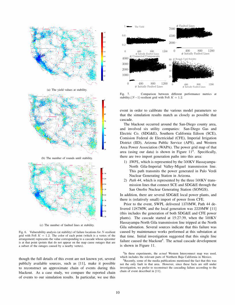
(a) The yield values at stability.

(b) The number of rounds until stability.

(c) The number of faulted lines at stability.

Fig. 6. Vulnerability analysis (at stability) of failure locations for N -resilientgrid with FoS K = 1.2. The color of each point (which is a vertex of thearrangement) represents the value corresponding to a cascade whose epicenteris at that point (points that do not appear on the map cause outages that area subset of the outages caused by a nearby vertex).

though the full details of this event are not known yet, severalpublicly available sources, such as [11], make it possibleto reconstruct an approximate chain of events during thisblackout. As a case study, we compare the reported chainof events to our simulation results. In particular, we use this

0 400 800 1200# Initially Faulted Lines

The Yield1

0.6

0.2

7000

4500

2000

0 400 800 1200# Initially Faulted Lines

# Faulted Lines

4000

3000

1000

0 400 800 1200# Initially Faulted Lines

# Connected Components

2000

80

60

40

0 400 800 1200

20

# Initially Faulted Lines

# Rounds Until Stability

Fig. 7. Comparison between different performance metrics atstability;(N−1)-resilient grid with FoS K = 1.2.

event in order to calibrate the various model parameters sothat the simulation results match as closely as possible thatcascade.

The blackout occurred around the San-Diego county area,and involved six utility companies: San-Diego Gas andElectric Co. (SDG&E), Southern California Edison (SCE),Comision Federal de Electricidad (CFE), Imperial IrrigationDistrict (IID), Arizona Public Service (APS), and WesternArea Power Association (WAPA). The power grid map of thatarea (using our data) is shown in Figure 114. Specifically,there are two import generation paths into this area:

1) SWPL, which is represented by the 500KV Hassayampa-North Gila-Imperial Valley-Miguel transmission line.This path transmits the power generated in Palo VerdiNuclear Generating Station in Arizona.

2) Path 44, which is represented by the three 500KV trans-mission lines that connect SCE and SDG&E through theSan Onofre Nuclear Generating Station (SONGS).

In addition, there are several SDG&E local power plants, andthere is (relatively small) import of power from CFE.

Prior to the event, SWPL delivered 1370MW, Path 44 de-livered 1287MW, and the local generation was 2229MW [11](this includes the generation of both SDG&E and CFE powerplants). The cascade started at 15:27:39, when the 500KVHassayampa-North Gila transmission line tripped at the NorthGila substation. Several sources indicate that this failure wascaused by maintenance works performed at this substation atthat time. Initial investigation suggested that this single linefailure caused the blackout5. The actual cascade developmentis shown in Figure 11.

4In these experiments, the actual Western Interconnect map was used,which includes the relevant parts of Northern Baja California in Mexico.

5Recently, some of the media publications mentioned the fact that this wasnot the only fault in that area. However, since these facts are still underinvestigation, we prefer to reconstruct the cascading failure according to thechain of event described in [11].

10

(a) The yield values at stability.

(b) The number of rounds until stability.

(c) The number of faulted lines at stability.

Fig. 8. Vulnerability analysis (at stability) of failure locations for an (N−1)-resilient grid with FoS K = 1.2. The color of each point (which is a vertexof the arrangement) represents the value corresponding to a cascade whoseepicenter is at that point.

B. Simulation Results

We performed two sets of experiments. In the first set,instead of performing simulation on the entire Western Inter-connect, we chose to use a part of the grid which includes onlythe affected area. The initial conditions were set to match asclose as possible the actual conditions prior to the event. Inparticular, we set the generation of the Palo Verde nuclearplant (which is the main contributing import generation unit)to 3,600 MW out of its nominal 4,300MW. This resulted

(a) (b)

0.04

0.01

0.02

0.03

0.6

0.2

0.4

0.1 0.2 0.3 0.4 0.5 0.1 0.2 0.3 0.4 0.50 0

ε ε

Average Yield Yield Standard Deviation

Fig. 9. The results for a representative failure epicenter, using stochasticoutage rule, based on 100 independent runs. (a) presents the average yield,while (b) presents its standard deviation.

Yield

0 5 10 15 20 25

0.2

0.4

0.6

0.8

1

Failure ID

deterministic

stochastic

Fig. 10. A comparison of the deterministic and stochastic outage rules forselected failure events.

Fig. 11. The development of the San Diego blackout according to [11].

in the following initial conditions of the import generation:SWPL = 1,386MW, Path 44 = 1,284MW.

Moreover, since in the actual event there was no (N − 1)-resilience with respect to the faulted North Gila–Hassyampaline, we used an N -resilient grid with different values ofFoS K (recall Section V-A). In addition, by [11], the actualcapacity of Path 44 is almost 2.7 times the flow in normaloperation. This information also correlates with other sources(e.g., [40]) which indicate that the power capacities are notbased on a uniform FoS parameter. Since Path 44 was a majorfactor of the cascade development, as it carried most of thelost SWPL power, we decided to adjust its FoS accordingly.In particular, its FoS was set to 2.5. After experimenting withthe value of K for other lines, we found out that K = 1.5leads to a behavior that most resembles that of the actual event. The resulting cascade behavior is shown in Figure 12.

Table II presents a brief comparison of the simulation resultsand the known details of the actual event. The description ofthe actual event is presented exactly as in [11], without anyinterpretation. It can be observed that although the simulatedcascade does not follow exactly the actual one, both of themdeveloped in a similar way. This suggests that our model anddata can be used to identify the vulnerable locations and design

11

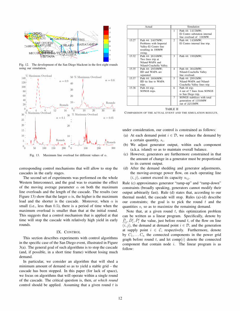
Fig. 12. The development of the San Diego blackout in the first eight roundsusing our simulation.

0 4 8 12 160

20

40

60

80

100

120

140

α = 0.9

% Maximum Overload

Rounds

α = 0.6

% Maximum Overload

Rounds

0 10 20 30 400

10

20

30

40

50

0 50 100 150 200

α = 0.1

% Maximum Overload

Rounds

0

5

10

15

20

25

30

α = 0.05

% Maximum Overload

Rounds

0 100 200 300

30

0

20

10

Fig. 13. Maximum line overload for different values of α.

corresponding control mechanisms that will allow to stop thecascades in the early stages.

The second set of experiments was performed on the wholeWestern Interconnect, and the goal was to examine the effectof the moving average parameter α on both the maximumline overloads and the length of the cascade. The results (seeFigure 13) show that the larger α is, the higher is the maximumload and the shorter is the cascade. Moreover, when α issmall (i.e., less than 0.5), there is a period of time when themaximum overload is smaller than that at the initial round.This suggests that a control mechanism that is applied at thattime will stop the cascade with relatively high yield in earlyrounds.

IX. CONTROL

This section describes experiments with control algorithmsin the specific case of the San Diego event, illustrated in Figure3(a). The general goal of such algorithms is to stop the cascade(and, if possible, in a short time frame) without losing muchdemand.

In particular, we consider an algorithm that will shed aminimum amount of demand so as to yield a stable grid – thecascade has been stopped. In this paper (for lack of space),we focus on algorithms that will operate within a single roundof the cascade. The critical question is, then, at which roundcontrol should be applied. Assuming that a given round t is

Actual Simulation1 Path 44: 1415MW;

El Centro substation internalline overload of 100MW.

15:27 Path 44: 2407MW; 2 Path 44: 1438MW;Problems with Imperial El Centro internal line trip.Valley-El Centro lineresulting in 100MWswing.

15:32 Path 44: 2616MW; 3 Path 44: 1992MW;Two lines trip atNiland-WAPA andNiland-Coachella Valley.

15:35 Path 44: 2959MW; 4 Path 44: 3043MW;IID and WAPA are Niland-Coachella Valleyseparated. line overload.

15:37 Path 44: 3006MW; 5 Path 44: 2991MW;IID tie line to WAPA Niland-WAPA and Niland-trips. Coachella Valley lines trip.

15:38 Path 44 trip; 6 Path 44 trip;SONGS trips. 4 out of 7 lines from SONGS

to San Diego trip.7 SONGS stabilizes with total

generation of 1350MWout of 2253MW.

TABLE IICOMPARISON OF THE ACTUAL EVENT AND THE SIMULATION RESULTS.

under consideration, our control is constrained as follows:(a) At each demand point i ∈ D, we reduce the demand by

a certain quantity, si.(b) We adjust generator output, within each component

(a.k.a. island) so as to maintain overall balance.(c) However, generators are furthermore constrained in that

the amount of change in a generator must be proportionalto its current output.

(d) After the demand shedding and generator adjustments,the moving-average power flow, on each operating line(i, j), cannot exceed its capacity uij .

Rule (c) approximates generator “ramp-up” and “ramp-down”constraints (broadly speaking, generators cannot modify theiroutput arbitrarily fast). Rule (d) states that, according to ourthermal model, the cascade will stop. Rules (a)-(d) describeour constraints; the goal is to pick the round t and thequantities si so as to maximize the remaining demand.

Note that, at a given round t, this optimization problemcan be written as a linear program. Specifically, denote byf tij , D

ti , P

ti the value, just before round t, of the flow on line

(i, j), the demand at demand point i ∈ D, and the generationat supply point i ∈ C, respectively. Furthermore, denoteby C1, . . . Cn the connected components in the power gridgraph before round t, and let comp(i) denote the connectedcomponent that contain node i. The linear program is asfollow:

12

Fig. 14. Illustration of cascading failures over 5 rounds using stochasticoutage rule with ε = 0.05, p = 0.5, and α = 0.1. The colors represent therounds in which the lines faulted.

minimize∑

i∈D si subject to

0 ≤ si ≤ Dti ∀i ∈ D

α|fij | + (1− α)f tij ≤ (1− ε)uij ∀ line (i, j)∑

(i,j)∈δ+(i) fij−∑

(j,i)∈δ−(i) fji=Pi, ∀i ∈ C∑(i,j)∈δ+(i) fij−

∑(j,i)∈δ−(i) fji=−(Dt

i−si) ∀i ∈ D∑(i,j)∈δ+(i) fij−

∑(j,i)∈δ−(i) fji=0, ∀i ∈ N\(C∪D)

θi − θj − xijfij = 0 ∀ line (i, j)0 ≤ λCm ≤ 1 ∀ component Cm

Pi = P ti (1− λcomp(i)) ∀i ∈ C∑

i∈Cm∩C Pi =∑

i∈Cm∩D Di ∀ component Cm

where, as in Section III, δ+(i) (δ−(i)) is the set of linesoriented out of (into) node i. Notice that third-sixth equationsin the linear program above are identical to Equations (1)-(2)in Section III.

As mentioned before, we demonstrate our control mecha-nism by considering a failure event in San Diego area. Figure14 presents the development of this event over the first fiverounds of a particular run obtained using the stochastic linefailure model with ε = 0.05, p = 0.5, and α = 0.1 (that is, asimulation with small time increments).

Table III outlines the performance of the optimal controlmechanism, where “Round” refers to the round on which theoptimal control is applied, while “Yield” refers to the outcome.We see from the table that applying control at the outset of thecascade is not optimal (this is typical, in our experience). Onthe other hand, waiting too long is not optimal either. Rather,there is a critical frame of time where effective control ispossible; the precise time frame can be discovered by runningour simulation upon the failure event, and applying the controlonly when we reach the round with optimal outcome. We alsonote that without control, the cascade stops at round 74 withthe yield of 0.34. Currently, we are developing robust versionsof this algorithm with respect to errors in data, timing, anddelays in implementation.

TABLE IIIOPTIMAL CONTROL OUTCOME.

Round 1 5 10 20 30 40 50 74Yield 0.22 0.55 0.49 0.41 0.39 0.38 0.36 0.34

X. CONCLUSION AND FUTURE WORK

In this paper, we considered a DC power flow and anaccompanied cascading failure model. We showed analyticallythat these models differ from previously-studied model basedon an epidemic-like failures (which are often analyzed usingpercolation theory). Then, we used techniques from optimiza-tion and computational geometry along with detailed GIS datato develop a method for identifying the power grid locationsthat are vulnerable to geographically correlated failures. Weperformed extensive numerical experiments that show therelations between the various parameters and performancemetrics. Specifically, we used a recent major blackout event inSan Diego area as a case study to calibrate different parametersof the simulations. We also demonstrated that the use ofcontrol at the right point in the cascade can mitigate the effectsof a large scale failure. While the presented results are for anintentionally modified version of the US Western Interconnect,they demonstrate the strength of our tools and provide insightsinto the issues affecting the resilience of the grid. These resultscan be used when designing new power grids, when makingdecisions regarding shielding or strengthening existing grids,and when determining the locations for deploying meteringequipment.

This is one of the first steps towards an understanding ofthe grid resilience to large scale failures. Hence, there arestill many open problems. For example, we plan to study theresults’ sensitivity to the failure model (e.g., to consider a ruleunder which the probability of a line failure is a function ofthe overload). Moreover, we plan to study the effectiveness ofsome of the current control algorithms and their capability tocope with geographically correlated failures. Finally, we planto develop control algorithms that will mitigate the effects ofsuch failures and network design tools that would enable toconstruct resilient grids.

ACKNOWLEDGEMENTS

This work was supported in part by DOE award DE-SC000267, the Legacy Heritage Fund program of the Is-rael Science Foundation (Grant No. 1816/10), DTRA grantHDTRA1-09-1-0057, a grant from the from the U.S.-IsraelBinational Science Foundation, and NSF grants CNS-10-18379 and CNS-10-54856. We thank Eric Glass for help withGIS data processing.

REFERENCES

[1] P. Agarwal, A. Efrat, A. Ganjugunte, D. Hay, S. Sankararaman, andG. Zussman, “The resilience of WDM networks to probabilistic geo-graphical failures,” in Proc. IEEE INFOCOM’11, Apr. 2011.

[2] M. Amin and P. F. Schewe, “Preventing blackouts: Building a smarterpower grid,” Scientific American, May 2007.

13

[3] G. Andersson, “Modelling and analysis of electric power sys-tems,” Lecture 227-0526-00, Power Systems Laboratory, ETH Zurich,March 2004, http://www.eeh.ee.ethz.ch/downloads/academics/courses/227-0526-00.pdf.

[4] M. Anghel, K. A. Werley, and A. E. Motter, “Stochastic model for powergrid dynamics,” in Proc. HICSS’07, Jan. 2007.

[5] K. Atkins, J. Chen, V. S. A. Kumar, and A. Marathe, “The structureof electrical networks: a graph theory-based analysis,” Int. J. CriticalInfrastructures, vol. 5, no. 3, pp. 265–284, 2009.

[6] A. R. Bergen and V. Vittal, Power Systems Analysis. Prentice-Hall,1999.

[7] D. Bienstock, “Optimal control of cascading power grid failures,” inPES General Meeting, July 2011.

[8] D. Bienstock and A. Verma, “The N − k problem in power grids:New models, formulations, and numerical experiments,” SIAM J. Optim.,vol. 20, no. 5, pp. 2352–2380, 2010.

[9] V. M. Bier, E. R. Gratz, N. Haphuriwat, W. Magua, and K. Wierzbicki,“Methodology for identifying near-optimal interdiction strategies for apower transmission system,” Reliab. Eng. Syst. Safety, vol. 92, pp. 1155–1161, 2007.

[10] R. Billinton and W. Li, Reliability Assessment of Electrical PowerSystems Using Monte Carlo Methods. Plenum Press, 1994.

[11] California Public Utilities Commission (CPUC), “CPUC briefing onSan Diego blackout,” http://media.signonsandiego.com/news/documents/2011/09/23/CPUC briefing on San Diego blackout.pdf.

[12] D. P. Chassin and C. Posse, “Evaluating north american electric gridreliability using the Barabsi–Albert network model,” Physica A, vol.355, no. 2-4, pp. 667 – 677, 2005.

[13] J. Chen, J. S. Thorp, and I. Dobson, “Cascading dynamics and mitigationassessment in power system disturbances via a hidden failure model,”Int. J. Elec. Power and Ener. Sys., vol. 27, no. 4, pp. 318 – 326, 2005.

[14] T. N. Dinh, Y. Xuan, M. T. Thai, E. K. Park, and T. Znati, “Onapproximation of new optimization methods for assessing networkvulnerability,” in Proc. IEEE INFOCOM’10, 2010.

[15] I. Dobson, “personal communication,” 2010.[16] I. Dobson, B. Carreras, V. Lynch, and D. Newman, “Complex systems

analysis of series of blackouts: cascading failure, critical points, andself-organization,” Chaos, vol. 17, no. 2, p. 026103, June 2007.

[17] W. R. Forstchen, One Second After. Forge Books, 2009.[18] J. S. Foster, E. Gjelde, W. R. Graham, R. J. Hermann, H. M. Kluepfel,

R. L. Lawson, G. K. Soper, L. L. Wood, and J. B. Woodard, “Reportof the commission to assess the threat to the United States fromelectromagnetic pulse (EMP) attack, critical national infrastructures,”Apr. 2008.

[19] H. Gharavi and R. Ghafurian, “Special issue on smart grid: The electricenergy system of the future,” Proc. IEEE., vol. 99, no. 6, 2011.

[20] Gurobi, “Optimizer,” http://www.gurobi.com/.[21] A. F. Hansen, A. Kvalbein, T. Cicic, and S. Gjessing, “Resilient routing

layers for network disaster planning,” in Proc. ICN’05, ser. LNCS,P. Lorenz and P. Dini, Eds. Springer, 2005, vol. 3421, pp. 1097–1105.

[22] P. Hines, K. Balasubramaniam, and E. Cotilla-Sanchez, “Cascadingfailures in power grids,” IEEE Potentials, vol. 28, no. 5, pp. 24–30,2009.

[23] P. Hines, E. Cotilla-Sanchez, and S. Blumsack, “Do topological modelsprovide good information about electricity infrastructure vulenrablity?”Chaos, vol. 20, no. 3, p. 033122, Sept. 2010.

[24] IBM, “ILOG CPLEX Optimizer,” http://www-01.ibm.com/software/integration/optimization/cplex-optimizer/.

[25] Z. Kong and E. M. Yeh, “Resilience to degree-dependent and cascadingnode failures in random geometric networks,” IEEE Trans. Inf. Theory,vol. 56, no. 11, pp. 5533–5546, Nov. 2010.

[26] Y.-C. Lai, A. Motter, and T. Nishikawa, “Attacks and cascades incomplex networks,” in Complex Networks, ser. Lecture Notes in Phys.,E. Ben-Naim, H. Frauenfelder, and Z. Toroczkai, Eds. Springer, 2004,vol. 650, pp. 299–310.

[27] J. Lavaei and S. Low, “Zero duality gap in optimal power flow problem,”to appear IEEE Trans. Power Syst., 2011.

[28] J. Lavaei, A. Rantzer, and S. H. Low, “Power flow optimization usingpositive quadratic programming,” in Proc. 18th IFAC World Congress,Aug. 2011.

[29] S. Neumayer, G. Zussman, R. Cohen, and E. Modiano, “Assessingthe vulnerability of the fiber infrastructure to disasters,” in Proc. IEEEINFOCOM’09, Apr. 2009.

[30] G. A. Pagani and M. Aiello, “The power grid as a complex network: asurvey,” ArXiv e-prints, May 2011.

[31] R. Pfitzner, K. Turitsyn, and M. Chertkov, “Controlled tripping ofoverheated lines mitigates power outages,” ArXiv e-prints, Oct. 2011.

[32] A. Pinar, J. Meza, V. Donde, and B. Lesieutre, “Optimization strategiesfor the vulnerability analysis of the electric power grid,” SIAM J. Optim.,vol. 20, no. 4, pp. 1786–1810, Feb. 2010.

[33] Platts, “GIS Data,” http://www.platts.com/Products/gisdata.[34] J. Salmeron, K. Wood, and R. Baldick, “Worst-case interdiction analysis

of large-scale electric power grids,” IEEE Trans. Power Syst., vol. 24,no. 1, pp. 96 –104, feb. 2009.

[35] C. M. Schneider, A. A. Moreirab, J. J. S. Andrade, S. Havlin, andH. J. Herrmann, “Mitigation of malicious attacks on networks,” inProceedings of the National Academy of Sciences of the United Statesof America, vol. 108, no. 10, Mar. 2011, pp. 3838 – 3841.

[36] A. Sen, S. Murthy, and S. Banerjee, “Region-based connectivity: a newparadigm for design of fault-tolerant networks,” in Proc. IEEE HPSR’09,Jun. 2009.

[37] U.S.-Canada Power System Outage Task Force, “Final report on theAugust 14, 2003 blackout in the United States and Canada: Causes andrecommendations,” Apr. 2004, https://reports.energy.gov.

[38] U.S. Federal Energy Regulatory Commission, Dept. of HomelandSecurity, and Dept. of Energy, “Detailed technical report on EMPand severe solar flare threats to the U.S. power grid,” Oct. 2010,http://www.ornl.gov/sci/ees/etsd/pes/.

[39] Z. Wang, A. Scaglione, and R. Thomas, “Generating statistically correctrandom topologies for testing smart grid communication and controlnetworks,” IEEE Trans. Smart Grid, vol. 1, no. 1, pp. 28 –39, June2010.

[40] Western Electricity Coordinating Council (WECC), “Historical trans-mission paths database,” http://www.wecc.biz.

[41] H. Xiao and E. M. Yeh, “Cascading link failure in the power grid: Apercolation-based analysis,” in Proc. IEEE Int. Work. on Smart GridCommun., June 2011.

APPENDIX

Proof of Observation 3.1: Let fei be the flow along lineei, let xei be its reactance and let θvi be the phase angle ofnode vi. By summing over the equalities of (2) for the linesof path p1 we get θa − θb =

∑ei∈p1

feixei . Similarly, for p2,θa − θb =

∑e′i∈p2

fe′ixe′i, and the claim follows.

Proof of Lemma 4.1: Consider an M -ring, and supposethat M is even (similar arguments can be used when M isodd). Assume that the capacity of all lines is 1, except lines(M/2,M + M/2 + 1) and (M/2,M + M/2 + 1)′ whosecapacity is 0.5. Assume also that α > 0. Initially, the ringoperates flawlessly, and all power flows are within the capacityof the corresponding lines.

Suppose that an initial failure event occur in lines (0,M)and (0,M)′ (that is, a parallel lines failure). As describedabove, all lines will either carry flow of 0 or of 1, and thereforeall lines except (M/2,M+M/2+1) and (M/2,M+M/2+1)′

will continue operating normally.As for lines (M/2,M+M/2+1) and (M/2,M+M/2+1)′,

their post-failure power flow is 1 while their pre-failure flowis 0.5. Since for each α > 0, α · 1 + (1 − α) · 0.5 > 0.5 =uM/2,M+M/2+1, these lines fault in the next round. Thus, thedistance between consecutive failures in this cascade is Θ(M).As one can choose an arbitrarily large M -ring, the distancebetween there two consecutive failures can be made arbitrarilylarge and the claim follows.

Proof of Lemma 4.2: When the power capacity u ofeach line is 0.5, the same failure described in the proof ofLemma 4.1, which starts with 2 lines failure, causes an outage

14

of 3/5 of the lines. Notice that in this case after the firstiteration there is a demand shedding of half the total demand.Only odd lines still operate and each one of them carries apower flow of 0.5 unit (which is below its power capacity).Thus, this specific failure event stops after one iteration.

Proof of Lemma 4.3: Consider an M -ring and assumethat the capacity of all lines is 0.5, and, for ease of presen-tation, that α = 1. Initially, the ring operates flawlessly, andall power flows are within the capacity of the correspondinglines.

Let A = {(0,M), (0,M)′} (parallel lines failure). Asdescribed above, after a single iteration, all tie lines and oddlines will carry power flow of 1 unit, exceeding their capacityand therefore faulting. This will cause a demand shedding of2 unit within Area 1 (no remaining active power lines); in therest of the areas there will be a demand shedding of 1 unit (odddemand node will be disconnected), resulting in a total demandshedding of M + 1, and a total yield of (M − 1)/2M < 0.5.

On the other hand, assume an area failure of Area 0. Clearly,the area failure is a superset of A. However, the area failureevent causes only demand shedding of 2 and therefore a yieldof (M − 1)/M > 0.5 (for every M > 2). The reason is thatin that case the cascade does not propagate outside Area 0,and all other power flows remain the same.

Proof of Lemma 4.4: Consider an M -ring and an M -ring with no tie-lines (which is a subgraph of the M -ring).Assume that the capacity of all lines is 0.5, and, for ease ofpresentation, that α = 1.

As we have shown before that a failure in {(0,M), (0,M)′}causes a yield less than 0.5 in the M -ring. On the other hand,when there are no tie-line, this failure is contained within Area1, resulting in a yield of at least (2M − 2)/2M > 0.5 (forM > 2). The same localization property holds for all othertypes of failures.

Proof of Lemma 4.5: Assume that the flow on line(0,M)′ is y. Thus, (1) and Observation 3.1 imply that theflow of each of the lines (0,M + 1) and (0,M + 1)′ is12 (2 − y) = 1 − y

2 . In addition, (1) implies that the flowon the tie line connecting Area 0 and Area 1 is 1− y.

Focus on Area 1. Similar arguments yield that the flow on(1,M+2) and (1,M+2)′ is y/2, the flow on (1,M+2) and(1,M+2)′ is 1−y/2 and the flow on the tie line is 1−y. Bysymmetry, the same flow assignment holds for all other areas.

Now consider two paths between node 0 and node M . Onetraverses the single line (0,M)′ that carries y unit of powerflow. The other traverses M tie lines, M odd lines, and M−1even lines; the power flow along even lines is in the oppositedirection. Thus, the total flow along this path is M(1− y) +M(1 − y/2) − (M − 1)(y/2) = 2M − 2My + y/2. Thus,by Observation 3.1, y = 2M − 2My + y/2 implying thaty = 2M

(0.5+2M) .Proof of Corollary 4.6: The proof follows by case

analysis. First, consider a failure event of a tie line. Sincethere is no power flow along the tie line, such a failure doesnot change the operations of the power grid and a capacityof 0.5 along internal lines and 0 along tie lines suffices to

11

Fig. 15. Illustration of the proof of Lemma 4.7. The graph Q4 has 4 pathsbetween its generation node and its demand node, two of length 2, one oflength 4, and one of length 8.

withstand such a failure.On the other hand, Lemma 4.5 analyzes a single internal

line failures. In that case, as M goes to infinity, the post-failure flow on an internal lines approaches 1. On the otherhand, the maximum post-failure flow on the tie lines is 1/9when M = 2.

Proof of Lemma 4.7: For any m > 2, let Qm = ⟨C∪D, E⟩be an undirected graph with a single supply node and a singledemand node, that are connected through m disjoint path in thefollowing manner: the first two paths are of length 2 (implyingthat along each of these path there is an additional intermediateneutral node, connected to the generator on one side and tothe demand node on the other side). For any i > 2, path iis of length 2i+1. See Figure 15 depicting Q4. Assume alsothat all lines have the same capacity u = 1/2 and the samereactance x = 1. We note that the total number of lines inQm is 2m and the total number of nodes is 2m −m+ 2.

By Observation 3.1, the sum of flows along each of them path is the same, denoted by y. In addition, since thereis no generation or demand along each path and since eachintermediate node has degree 2, (1) immediately implies thatall lines along the same path carry the same amount of flow.Namely, the flow along the lines of the first two path is y/2and for each line of path i (i > 2) the flow is y/2i−1. Solving(1) for the demand node, implies that y/2 +

∑m−1i=1 y/2i = 1

and therefore y = 11.5− 1

2m−1< 1 (for any m > 2). Since

the largest amount of flow on any line in the graph is y/2 <1/2 = u, there power initially flow flawlessly.

Suppose now that there is a failure event in one of the linesalong the first path. Applying (1) on the intermediate nodeimplies that there is no flow along the other line of that path.We next show that this failure event causes a cascade that lastm iterations, implying that cascades can be made arbitrarilylarge (by choosing larger graph Qm).

After each iteration ℓ, denote by yℓ the total amount of flowon each of the remaining path. We next show by inductionthat the flow yℓ+1/2

ℓ along each of the edges of the (ℓ+1)-thpath exceeds 1/2, implying that these lines fault in the nextiteration. In addition, for each j > ℓ + 1 the flow along alllines of the j-th path is less than 1/2, implying that they stilloperate at the end of the iteration.

In the base case, (1) for the demand node implies that∑m−1i=1 y1/2

i = 1, and therefore y1 = 11− 1

2m−1> 1, thus the

lines along the second path have power flow of y1/2 > 1/2

15

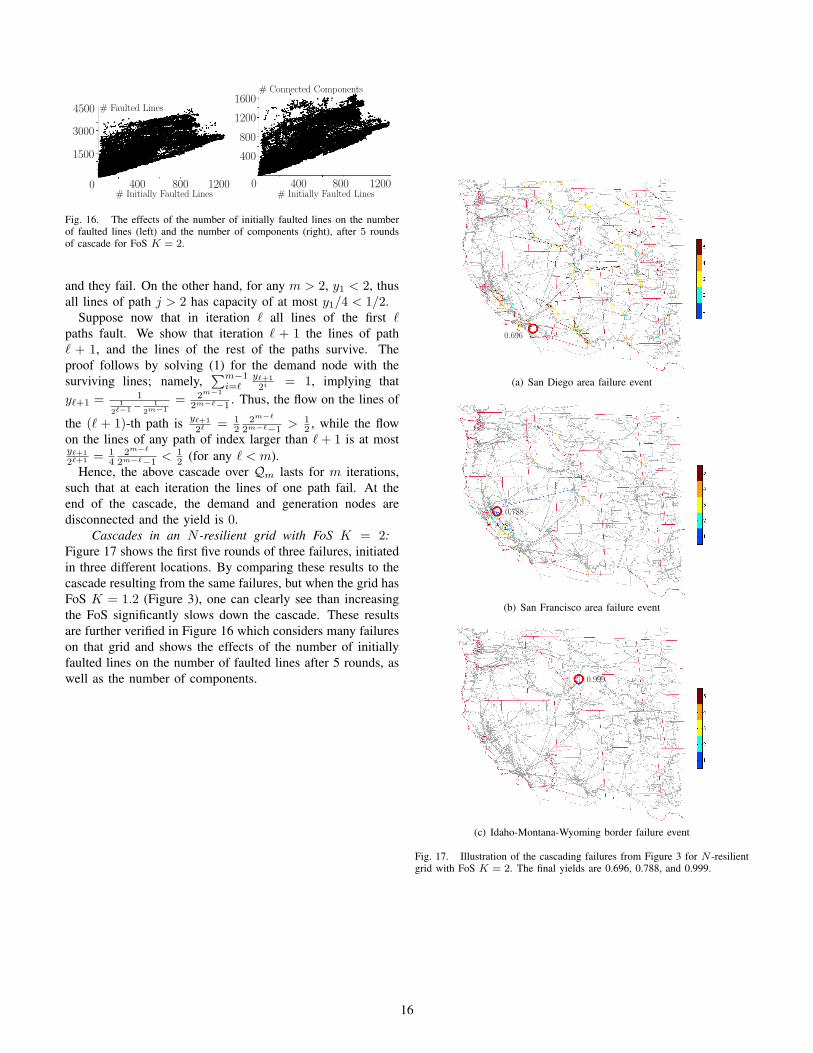
4500

3000

1500

0 400 800 1200# Initially Faulted Lines

# Faulted Lines1200

800

400

0 400 800 1200# Initially Faulted Lines

# Connected Components1600

Fig. 16. The effects of the number of initially faulted lines on the numberof faulted lines (left) and the number of components (right), after 5 roundsof cascade for FoS K = 2.

and they fail. On the other hand, for any m > 2, y1 < 2, thusall lines of path j > 2 has capacity of at most y1/4 < 1/2.

Suppose now that in iteration ℓ all lines of the first ℓpaths fault. We show that iteration ℓ + 1 the lines of pathℓ + 1, and the lines of the rest of the paths survive. Theproof follows by solving (1) for the demand node with thesurviving lines; namely,

∑m−1i=ℓ

yℓ+1

2i = 1, implying thatyℓ+1 = 1

1

2ℓ−1 − 1

2m−1= 2m−1

2m−ℓ−1. Thus, the flow on the lines of

the (ℓ + 1)-th path is yℓ+1

2ℓ= 1

22m−ℓ

2m−ℓ−1> 1

2 , while the flowon the lines of any path of index larger than ℓ+ 1 is at mostyℓ+1

2ℓ+1 = 14

2m−ℓ

2m−ℓ−1< 1

2 (for any ℓ < m).Hence, the above cascade over Qm lasts for m iterations,

such that at each iteration the lines of one path fail. At theend of the cascade, the demand and generation nodes aredisconnected and the yield is 0.

Cascades in an N -resilient grid with FoS K = 2:Figure 17 shows the first five rounds of three failures, initiatedin three different locations. By comparing these results to thecascade resulting from the same failures, but when the grid hasFoS K = 1.2 (Figure 3), one can clearly see than increasingthe FoS significantly slows down the cascade. These resultsare further verified in Figure 16 which considers many failureson that grid and shows the effects of the number of initiallyfaulted lines on the number of faulted lines after 5 rounds, aswell as the number of components.

0.696

(a) San Diego area failure event

0.788

(b) San Francisco area failure event

0.999

(c) Idaho-Montana-Wyoming border failure event

Fig. 17. Illustration of the cascading failures from Figure 3 for N -resilientgrid with FoS K = 2. The final yields are 0.696, 0.788, and 0.999.

16