Power Efficient Range Assignment for Symmetric Connectivity in

Static Ad Hoc Wireless Networks∗

E. Althaus† G. Calinescu‡ I.I. Mandoiu§ S. Prasad¶ N. Tchervenski‡

A.Zelikovsky¶

Abstract

In this paper we study the problem of assigning transmission ranges to the nodes of a static ad hoc wireless

network so as to minimize the total power consumed under the constraint that enough power is provided to the nodes

to ensure that the network is connected. We focus on the MIN-POWER SYMMETRIC CONNECTIVITY problem, in

which the bidirectional links established by the transmission ranges are required to form a connected graph.

Implicit in previous work on transmission range assignment under asymmetric connectivity requirements is the

proof that MIN-POWER SYMMETRIC CONNECTIVITY is NP-hard and that the MST algorithm has a performance

ratio of 2. In this paper we make the following contributions: (1) we show that the related MIN-POWER SYMMETRIC

UNICAST problem can be solved efficiently by a shortest-path computation in an appropriately constructed auxiliary

graph; (2) we give an exact branch and cut algorithm based on a new integer linear program formulation solving

instances with up to 35-40 nodes in 1 hour; (3) we establish the similarity between MIN-POWER SYMMETRIC

CONNECTIVITY and the classic STEINER TREE problem in graphs, and use this similarity to give a polynomial-time

approximation scheme with performance ratio approaching 5/3 as well as a more practical approximation algorithm

with approximation factor 11/6; and (4) we give the results of a comprehensive experimental study comparing new

and previously proposed heuristics with the above exact and approximation algorithms.

∗Preliminary versions of the results in this paper have appeared in [1, 11].†Max-Planck-Institut fur Informatik, Stuhlsatzenhausweg 85, D-66123 Saarbrucken, Germany. E-mail: althaus@mpi-sb.mpg.de.‡Department of Computer Science, Illinois Institute of Technology, Chicago, IL 60616. E-mail: {calinesc,tchenic}@iit.edu. Research of GC

was partially performed while visiting the Department of Combinatorial Optimization of University of Waterloo, where supported by a NSERC

grant, and partially performed while visiting the Max-Planck-Institut fur Informatik, Saarbrucken, Germany. Research of GC and NT supported in

part by an ERIF grant from the Illinois Institute of Technology.§Computer Science and Engineering Department, University of Connecticut, 371 Fairfield Rd., Unit 1155, Storrs, CT 06269. E-mail:

ion@engr.uconn.edu. The research of IIM was partially performed while the author was with the Departments of Computer Science and Engi-

neering and of Electrical and Computer engineering of the University of California at San Diego, La Jolla, CA.¶Department of Computer Science, Georgia State University, Atlanta, GA 30303. E-mail: {sprasad,alexz}@cs.gsu.edu. SP and AZ were

partially supported by the State of Georgia’s Yamacraw Initiative. AZ was also partially supported by NSF Grant CCR-9988331, Award No.

MM2-3018 of MRDA and CRDF.

1

1 Introduction

Ad hoc wireless networks have received significant attention in recent years due to their potential applications in

battlefield, emergency disaster relief, and other application scenarios (see, e.g., [3, 8, 9, 16, 18, 22, 26, 30, 29]).

Unlike wired networks or cellular networks, no wired backbone infrastructure is installed in ad hoc wireless networks.

A communication session is achieved either through single-hop transmission if the recipient is within the transmission

range of the source node, or by relaying through intermediate nodes otherwise. We assume that omnidirectional

antennas are used by all nodes to transmit and receive signals. Thus, a transmission made by a node can be received

by all nodes within its transmission range. This feature is extremely useful for energy-efficient multicast and broadcast

communications.

For the purpose of energy conservation, each node can (possibly dynamically) adjust its transmitting power, based

on the distance to the receiving node and the background noise. In the most common power-attenuation model [23], the

signal power falls as 1rκ where r is the distance from the transmitter antenna and κ is a real constant dependent on the

wireless environment, typically between 2 and 4. Assume that all receivers have the same power threshold for signal

detection, which is typically normalized to one. With this assumption, the power required to support a link between two

nodes separated by a distance r is rκ. A crucial issue is how to find a route with minimum total energy consumption

for a given communication session. This problem is referred to as Minimum-Energy Routing in [26, 30]. Having

every link established in both directions simplifies the one-hop transmission protocols by allowing acknowledgment

messages to be sent back for every packet (see, for example [27]). This motivates the study of the MIN-POWER

SYMMETRIC CONNECTIVITY problem, where a link is established only if both nodes have transmission range at least

as big as the distance between them, and we must ensure that established links form a connected network. Like in

[3], in this paper the objective is to minimize the total power assigned to the nodes; previous research on symmetric

connectivity has also addressed the objective of minimizing the maximum node power [18, 22].

Formally, given a set of points V (representing the nodes in the network) in E 2 (the two-dimensional Euclidean

space) or in E3 (the three-dimensional Euclidean space), a transmission range assignment (or range assignment, for

short) is a function r : V → R+. A unidirectional link from node u to node v is established under the range assignment

r if r(u) ≥ ‖uv‖, where ‖uv‖ denotes the Euclidean distance between u and v. A bidirectional link uv is established

under the range assignment r if r(u) ≥ ‖uv‖ and r(v) ≥ ‖uv‖. Let B(r) denote the set of all bidirectional links

established between pairs of nodes in V under the range assignment r. In this paper we study the following problem:

MIN-POWER SYMMETRIC CONNECTIVITY: Given a set of nodes V and κ ≥ 1, find a transmission range assignment

r : V → R+ minimizing∑

v∈V r(v)κ subject to the constraint that the graph (V, B(r)) is connected.

Implicit in the work of Clementi, Penna, and Silvestri [9] is a proof that MIN-POWER SYMMETRIC CONNECTIV-

ITY in E2 is NP-Hard (radio “bridges” in canonical form gadgets, see Definition 3 on page 10 of [9], can be made to

be bidirectional links). Also implicit in [9] is the proof that, in E 3 and in the graph model, MIN-POWER SYMMETRIC

CONNECTIVITY is APX-complete, and therefore, unless P = NP , does not admit a polynomial-time approximation

2

scheme. Thus, we search for polynomial-time constant approximation factor algorithms for this problem. The ap-

proximation factor, or performance ratio, of approximation algorithm A for a minimization problem is the supremum,

over all possible instances I , of the ratio between the cost of the output of A when running on I and the cost of an

optimal solution for I (the smaller the performance ratio, the better). We say that A is an α-approximation algorithm

if its performance ratio is at most α. A fully polynomial α-approximation scheme is a family of algorithms A ε such

that, for every ε > 0, algorithm Aε (1) has performance ratio at most α + ε, and (2) runs in time polynomial in the

size of the instance and 1/ε.

Kirousis, Kranakis, Krizanc, and Pelc [16] give a minimum spanning tree (MST) based 2-approximation algorithm

for MIN-POWER SYMMETRIC CONNECTIVITY (their algorithm is actually designed for a related problem, which we

discuss in Section 2). In this paper we improve the performance ratio under 2 by exploiting similarities between

MIN-POWER SYMMETRIC CONNECTIVITY and the classic STEINER TREE problem: given an edge-weighted graph

G = (V, E, w) and a set T ⊆ V of terminals, find a minimum weight Steiner tree for T , i.e., a minimum weight

connected subgraph of G which contains T . It is well known that computing an MST in the complete graph on T

with edge-weights equal to the minimum distance in G between corresponding terminals gives a 2-approximation

algorithm for STEINER TREE [6, 17]. Zelikovsky [31] gave the first algorithm with performance ratio less than 2: he

used 3-restricted Steiner trees and the concept of gain to obtain a performance ratio of 11/6. Promel and Steger [21]

extend the results of Camerini, Galbiati, and Maffioli [5] and give a polynomial time 5/3-approximation scheme for

STEINER TREE, by finding an almost optimal 3-restricted Steiner tree.

We show that similar concepts can be used for approximating MIN-POWER SYMMETRIC CONNECTIVITY. In

particular, we show that the algorithms of [21], [31], [2], and [32] can be modified to give similar performance ratios

for MIN-POWER SYMMETRIC CONNECTIVITY. Our main results are a fully polynomial 5/3 approximation scheme

based on [21], and a more practical algorithm with approximation factor of 11/6 [31].

Our algorithms have the same approximation guarantees when network nodes are located in E 3. In fact, since

they work on a graph model of the network, our algorithms can be applied to more general problem formulations,

e.g., observing given upper-bounds on the transmission range of each node and/or taking into account obstacles that

completely block the communication between certain pair of nodes.

The rest of the paper is organized as follows. In Section 2 we discuss several connectivity problems under both

symmetric and asymmetric connectivity models. In particular, we show that the MIN-POWER SYMMETRIC UNICAST

problem (which, for given source and destination nodes, s, t ∈ V , asks for a sequence v 0 = s, v1, . . . , vk = t of

nodes and transmission ranges r(vi), i = 0, . . . , k, under which all bidirectional links vivi+1 are established) can

be solved efficiently by a shortest-path computation in an appropriately constructed auxiliary graph. In Section 3 we

give a new integer program formulation for the MIN-POWER SYMMETRIC CONNECTIVITY problem, and describe an

exact branch and cut algorithm based on this formulation. Experimental results show that the branch and cut algorithm

solves instances with 25 nodes in less than one minute and instances with up to 35-40 nodes in 1 hour. In Section 4 we

show that the MST algorithm has a tight approximation factor of 2 for the MIN-POWER SYMMETRIC CONNECTIVITY

3

problem, and discuss modifications of the MST algorithm for handling given bounds on node transmission ranges. In

Section 5 we give a number of approximation algorithms for MIN-POWER SYMMETRIC CONNECTIVITY based on

the concept of k-restricted decomposition and the similarity to computing k-restricted Steiner trees. In Section 6 we

present the results of a comprehensive experimental study comparing new and previously proposed heuristics with the

above exact and approximation algorithms. The results show that best performing algorithms give an average of 5-6%

reduction in power consumption compared to the simple MST based solution. We conclude in Section 7 with open

problems and directions for future research.

2 Symmetric vs. Asymmetric Connectivity Problem Formulations

Several problems have been previously studied under the related asymmetric connectivity model, in which unidirec-

tional links give raise to a directed graph on V . In this section we discuss these formulations and compare them with

the corresponding symmetric connectivity variants.

2.1 Complete Network Connectivity

In the MIN-POWER ASYMMETRIC CONNECTIVITY problem (also referred to as the complete range assignment

problem) the objective is establishing a strongly connected subgraph of V . Kirousis, Kranakis, Krizanc, and Pelc [16]

prove that MIN-POWER ASYMMETRIC CONNECTIVITY in E3 is NP-Hard and, based on the minimum spanning tree,

give a 2-approximation algorithm. As opposed to the MIN-POWER ASYMMETRIC BROADCAST approximation of

[29], the MIN-POWER ASYMMETRIC CONNECTIVITY approximation of [16] is valid in arbitrary graphs (that is, the

distance between two points could be arbitrary, not necessarily Euclidean). Clementi, Penna, and Silvestri [9] give an

elaborate reduction proving that MIN-POWER ASYMMETRIC CONNECTIVITY in E 2 is also NP-Hard.

The power for the MIN-POWER ASYMMETRIC CONNECTIVITY can be half the power for MIN-POWER SYM-

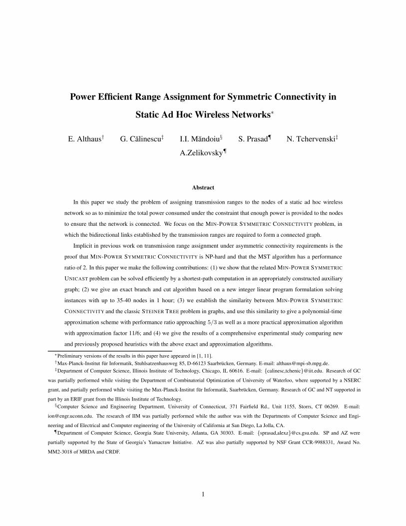
METRIC CONNECTIVITY as illustrated by the following example in which κ = 2. The terminal set (see Figure 1)

consists of n groups of n + 1 points each, located on the sides of a regular 2n-gon. Each group has 2 terminals in

distance 1 of each other (represented as thick circles in Figure 1) and n− 1 equally spaced points (dashes in Figure 1)

on the line segment between them. It is easy to see that the minimum range assignment ensuring asymmetric connec-

tivity assigns a power of 1 to the one thick terminal in each group and a power of ε 2 = (1/n)2 to all other points in

the group. The total power then equals n + 1. For symmetric connectivity it is necessary to assign power of 1 to all

but two of the thick points, and of ε2 to the remaining points, which results in total power of 2n − 1 − 1/n + 2/n2.

2.2 Unicast

The MIN-POWER ASYMMETRIC UNICAST problem requires establishing a minimum power directed path from a

source s to a destination t, and is easily solved in polynomial time by shortest-path algorithms. Below we reformulate

4

ε2ε2

ε ε ε ε ε ε

εεεε 1/n

1

ε=

1

1 1

1

1

1

1 1

1

n times

(b)

1

1ε ε ε ε ε ε

εεεε 1/n

1

ε=

ε

1

2

1 1

1

1

1

1 1

1

n times

(a)

1

Figure 1: Total power for the MIN-POWER ASYMMETRIC CONNECTIVITY can be half the total power for MIN-

POWER SYMMETRIC CONNECTIVITY (κ = 2). (a) Minimum range assignment ensuring asymmetric connectivity

has total power n + n2ε2 = n + n2 1n2 = n + 1. (b) Minimum range assignment ensuring symmetric connectivity has

the total power (2n − 2) + (n2 − n + 2)ε2 = 2n− 1 − 1n + 2

n2 .

MIN-POWER SYMMETRIC UNICAST as a graph problem, and then reduce the latter problem to a single-source single-

sink shortest-path computation in an appropriately constructed graph.

Let G = (V, E, c) be an edge-weighted graph and uv denote the undirected edge between nodes u and v. The cost

c(uv) of an edge uv ∈ E corresponds to the (symmetric) power requirement p(u, v) = p(v, u). The power cost of an

s–t path P = (s = v0, v1, . . . , vk = t) is p(P ) = c(v0v1) + c(vk−1vk) +∑k−1

i=1 max (c(vi−1vi), c(vi, vi+1)). The

MIN-POWER SYMMETRIC UNICAST can thus be reformulated as follows: Given a graph G = (V, E, c) with costs

on edges a source s ∈ V and a destination t ∈ V , find an s–t path in G of the minimum power-cost.

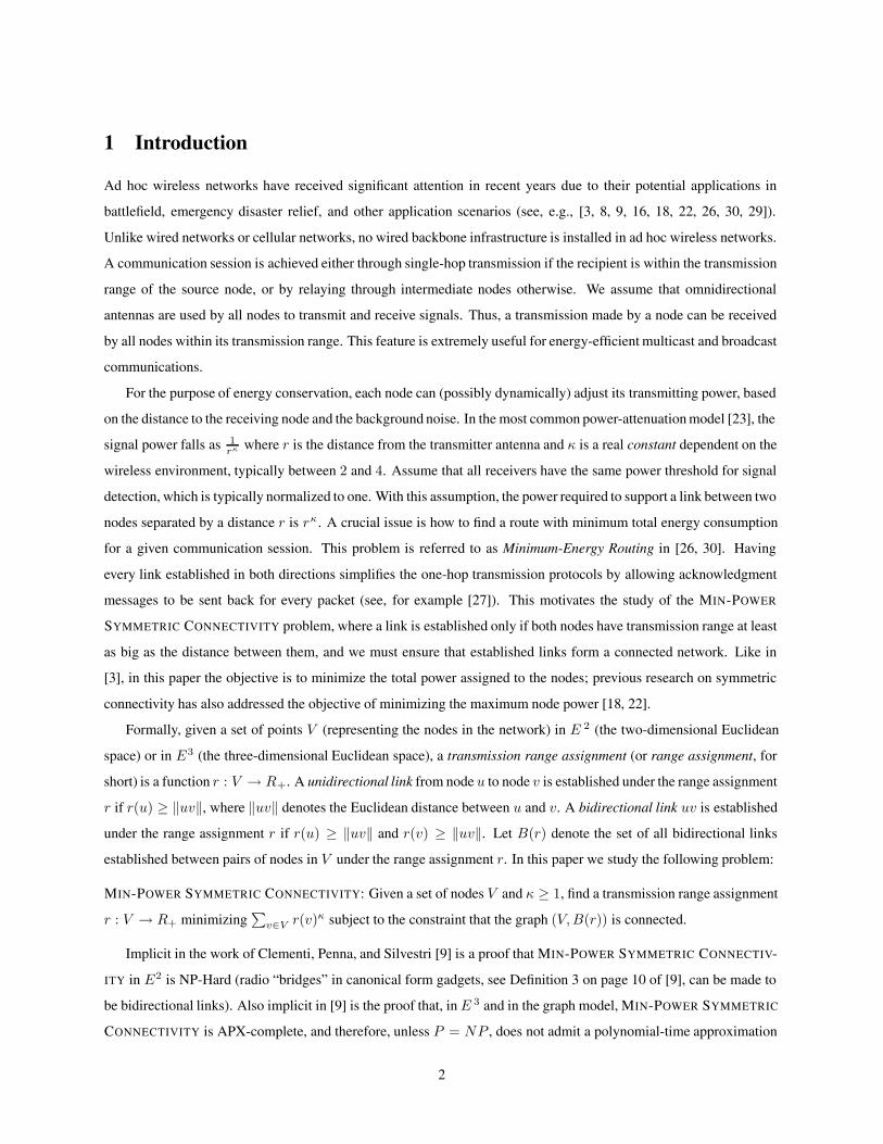
The following example in the Euclidean plane shows that a straightforward application of Dijkstra’s algorithm does

not work, i.e., a minimum cost s–t path does not always have minimum power-cost. Consider a network consisting of

three nodes, s = (0, 3), t = (4, 0), and x = (0, 0) (see Figure 2). If κ = 2, then the two s–t paths, namely, (s, t) and

(s, v, t), have the same cost of 25 but different power-costs: the power-cost of (s, t) is 25+25=50 while the power-cost

of (s, v, t) is 9+16+16=41.

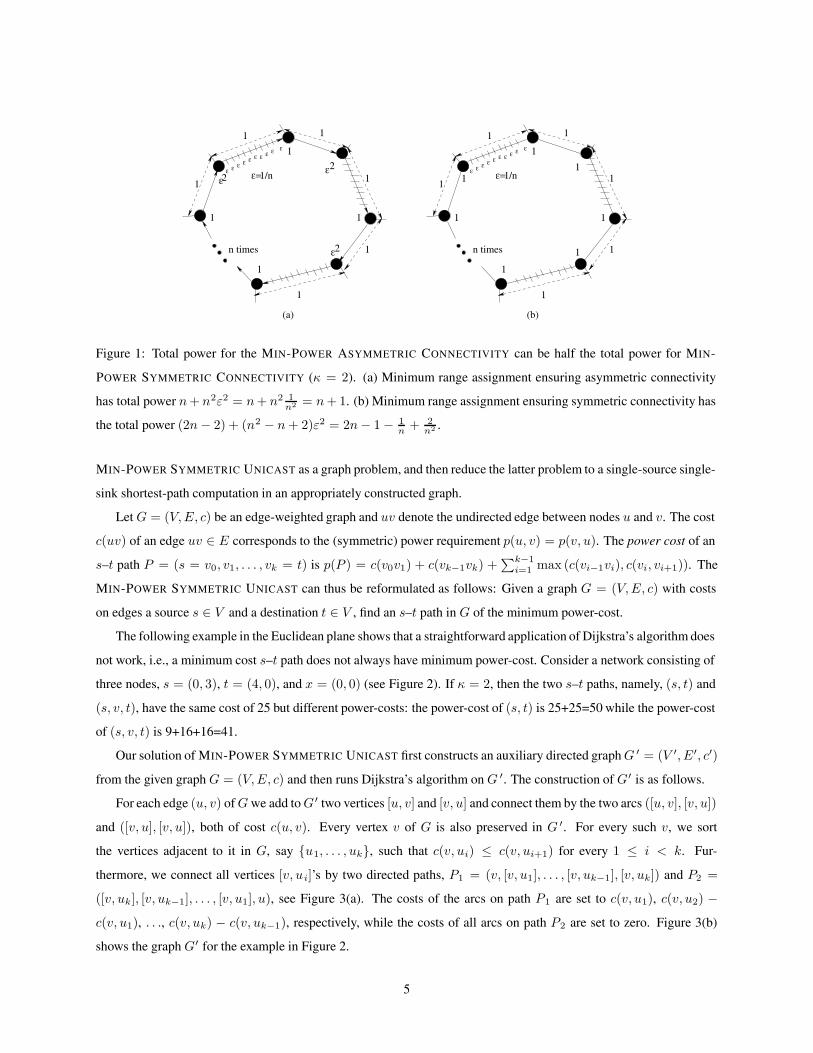
Our solution of MIN-POWER SYMMETRIC UNICAST first constructs an auxiliary directed graph G ′ = (V ′, E′, c′)

from the given graph G = (V, E, c) and then runs Dijkstra’s algorithm on G ′. The construction of G′ is as follows.

For each edge (u, v) of G we add to G′ two vertices [u, v] and [v, u] and connect them by the two arcs ([u, v], [v, u])

and ([v, u], [v, u]), both of cost c(u, v). Every vertex v of G is also preserved in G ′. For every such v, we sort

the vertices adjacent to it in G, say {u1, . . . , uk}, such that c(v, ui) ≤ c(v, ui+1) for every 1 ≤ i < k. Fur-

thermore, we connect all vertices [v, ui]’s by two directed paths, P1 = (v, [v, u1], . . . , [v, uk−1], [v, uk]) and P2 =

([v, uk], [v, uk−1], . . . , [v, u1], u), see Figure 3(a). The costs of the arcs on path P1 are set to c(v, u1), c(v, u2) −c(v, u1), . . ., c(v, uk) − c(v, uk−1), respectively, while the costs of all arcs on path P2 are set to zero. Figure 3(b)

shows the graph G′ for the example in Figure 2.

5

(b)(a)

9

16 160 25

25s

vt t

s

v

25 9

16

Figure 2: An example of two paths with the same cost and different power-costs. (a) The path (s, t) assigns powers

25 to s and to t. (b) The path (s, v, t) assigns powers 9 to s and 16 to v and t.

1

2 1

7

k-19

k

1

9

2

ck

9 9

16

16

16

9

16

u1 2u

u k

uk-1ck-1

2525

0

2

0

1

k-1

k

0

c -

c

c

v

c

v

[v,u ]

(a)

[v,u ]

[v,u ]

[v,u ]

s

c

[t,s]

t

(b)

v

c -c

[v,s]

[s,v] [s,t]

[v,t] [t,v]

Figure 3: (a) A vertex v adjacent to k vertices u1, . . . , uk via edges of cost c1, c2, . . . , ck and a gadget replacing v

with a bidirectional path. The solid edges of the path (v, [v, u2]), ([v, u2]), [v, u3],. . ., ([v, uk−1], [v, uk] have cost c1,

c2 − c1, . . ., ck − ck−1, respectively. The dashed edges have zero cost. (b) The graph G ′ for the example in Figure 2.

Thick edges belong to the shortest path corresponding to the path (s, v, t) in G.

6

We claim that every directed s–t path P in G corresponds to an s–t path P ′ in G′ whose cost is equal to the

power-cost of P . Indeed, consider a directed path P = (s = w1, w2, . . . , wl = t) in G. By construction, there exists

a directed path P ′ of G′ visiting, in order, vertices w1, [w1, w2], [w2, w1], . . ., [wl−1, wl], [wl, wl−1], wl, such that

• The cost of the arc connecting w1 to [w1, w2] in P ′ is c(w1, w2);

• The cost of the arc connecting [wi−1, wi] to [wi, wi−1] in P ′ plus the cost of the subpath connecting [wi, wi−1]

to [wi, wi+1] in P ′ is equal to max{c(wi−1, wi), c(wi, wi+1)} for every 2 ≤ i < l;

• The cost of the arc connecting [wl−1, wl] to [wl, wl−1] is c(wl−1, wl); and

• The cost of the subpath connecting [w l, wl−1] to wl is 0.

Therefore, the cost of P ′ equals the power-cost of P . It is not difficult to see that minimum power-cost paths in G

are necessarily mapped by this correspondence to shortest paths in G ′ and thus MIN-POWER SYMMETRIC UNICAST

reduces to computing a shortest path in G ′.

Using the Fibonacci heaps implementation of Dijkstra’s algorithm [10] to compute a shortest s–t path in G ′, and

observing that |V ′| = O(|V | + |E|) = O(|E|) and |E ′| = O(|E|), we obtain the following:

Theorem 1 MIN-POWER SYMMETRIC UNICAST is solvable in time O(|E| log |V |).

Even in E2, we have examples where the auxiliary graph is not planar, and we do not know faster methods to

compute shortest paths in this auxiliary graph. When edge costs are integers we can use Thorup’s single-source

shortest path algorithm [28], reducing the runtime to O(|V ′| + |E′|) = O(|E|).

2.3 Broadcast and Multicast

The MIN-POWER ASYMMETRIC BROADCAST problem [26, 30] requires establishing a minimum power arbores-

cence rooted at a given vertex s. Clementi et al. [8] prove that MIN-POWER ASYMMETRIC BROADCAST is NP-Hard

when the nodes are in E2. The best known approximation algorithm for MIN-POWER ASYMMETRIC BROADCAST

[29], based on computing a minimum spanning tree, has performance ratio of at most 12 when the nodes are in

E2. We remark that, due to the need of establishing bidirectional connections, MIN-POWER SYMMETRIC BROAD-

CAST and MIN-POWER SYMMETRIC CONNECTIVITY are the same problem. Implicit in the work of Kirousis,

Kranakis, Krizanc, and Pelc [16] is the result that computing an MST gives a 2-approximation for MIN-POWER

SYMMETRIC CONNECTIVITY, even in its graph formulation (see Theorem 2). In contrast, the graph version of

MIN-POWER ASYMMETRIC BROADCAST cannot be approximated within a factor better than (1 − o(1)) ln n unless

NP ⊆ TIME(nO(log log n)) [14].

In MIN-POWER ASYMMETRIC MULTICAST, one is given a root s and a set of terminals T , and the goal is to

establish a minimum-power branching rooted at s which reaches all vertices of T . As a generalization of MIN-POWER

7

ASYMMETRIC BROADCAST, MIN-POWER ASYMMETRIC MULTICAST is also NP-Hard, and the same method as in

[29] implies that an approximate minimum Steiner tree gives a performance ratio of 12ρ, where ρ is the approximation

for Steiner tree in graphs (the best result known at this moment, given in [24], is ρ = 1 + 12 ln 3 + ε).

No previous results have been published for the multicast problem under the symmetric connectivity model. An

immediate consequence of Theorem 2 is that a ρ-approximate minimum Steiner tree gives a performance ratio of 2ρ

for MIN-POWER SYMMETRIC MULTICAST.

3 Integer Linear Program Formulation

In this section we give an integer linear program (ILP) formulation for MIN-POWER SYMMETRIC CONNECTIVITY

and describe a branch and cut algorithm based on it. The results in Section 6 show that the algorithm is practical for

instances with up to 35-40 nodes.

We begin by reformulating MIN-POWER SYMMETRIC CONNECTIVITY in graph theoretical terms. Let G =

(V, E, c) be an edge-weighted graph and uv denote the undirected edge between nodes u and v. The cost c(uv) of an

edge uv ∈ E corresponds to the (symmetric) power requirement p(u, v) = p(v, u). For a node u ∈ V and a spanning

tree T of G, let uuT be the maximum cost edge incident to u in T , i.e., uuT ∈ T and c(uuT ) ≥ c(uv) for all uv ∈ T .

The power cost of a spanning tree T is

p(T ) =∑u∈V

c(uuT )

Since every connected graph contains a spanning tree, an equivalent formulation of MIN-POWER SYMMETRIC CON-

NECTIVITY is to ask for a spanning tree with minimum power-cost in the complete graph on V with edge costs given

by c(uv) = ‖uv‖κ. Thus, MIN-POWER SYMMETRIC CONNECTIVITY can be reformulated as follows: Given a

connected edge-weighted graph G = (V, E, c), find a spanning tree T of G with minimum power-cost.

To formulate the problem as a linear integer program, we use two types of binary decision variables:

• xuv for all uv ∈ E; xuv is set to 1 if uv belongs to the selected spanning tree T and to 0 otherwise. We call

these variables the tree variables; and

• yuv for all uv ∈ E := {uv, vu | uv ∈ E}; yuv is set to 1 if uT = v (i.e., if uv ∈ T and c(uv) ≥ c(uw) for all

uw ∈ T ) and to 0 otherwise. We call these variables the range variables.

Note that there are |E| tree variables and |E| = 2|E| range variables. Let ST be set of the incidence vectors of all

spanning trees of G (viewed as subsets of E). Our ILP formulation is as follows.

min∑

uv∈E

c(uv)yuv

s.t.∑

v∈V |uv∈E

yuv = 1, ∀u ∈ V (1)

8

����

��������

������ ��

����

��

��

�� ��

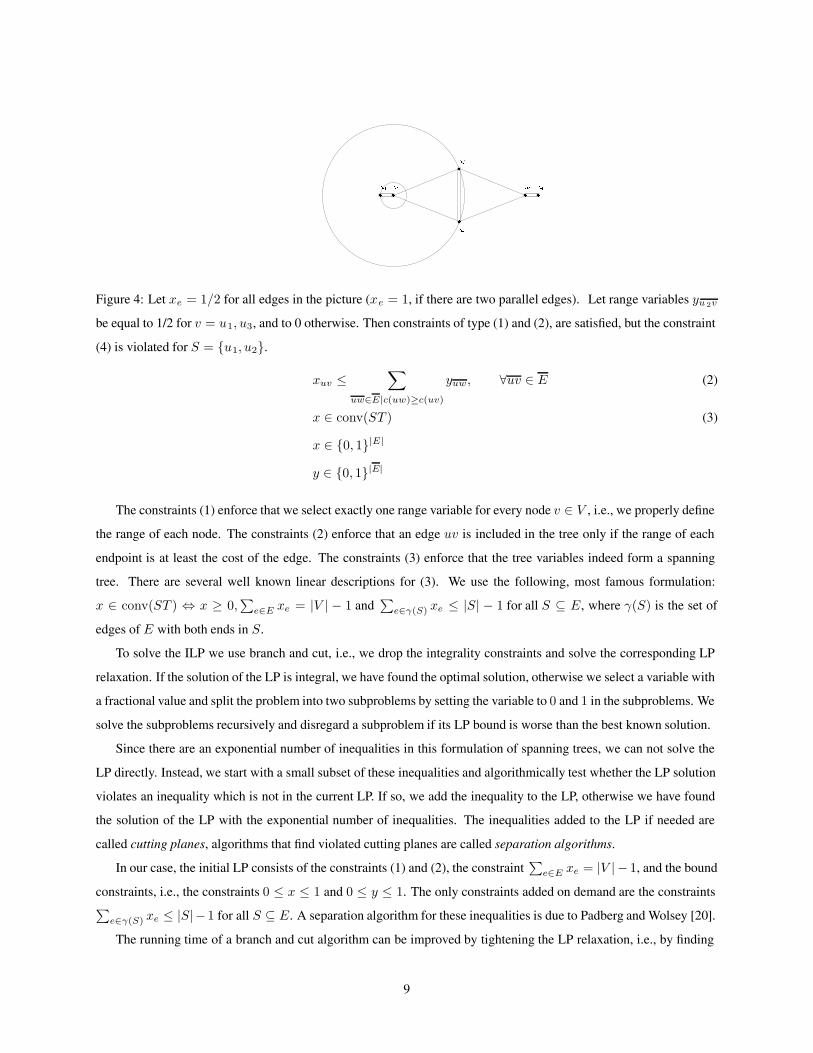
Figure 4: Let xe = 1/2 for all edges in the picture (xe = 1, if there are two parallel edges). Let range variables yu 2v

be equal to 1/2 for v = u1, u3, and to 0 otherwise. Then constraints of type (1) and (2), are satisfied, but the constraint

(4) is violated for S = {u1, u2}.

xuv ≤∑

uw∈E|c(uw)≥c(uv)

yuw, ∀uv ∈ E (2)

x ∈ conv(ST ) (3)

x ∈ {0, 1}|E|

y ∈ {0, 1}|E|

The constraints (1) enforce that we select exactly one range variable for every node v ∈ V , i.e., we properly define

the range of each node. The constraints (2) enforce that an edge uv is included in the tree only if the range of each

endpoint is at least the cost of the edge. The constraints (3) enforce that the tree variables indeed form a spanning

tree. There are several well known linear descriptions for (3). We use the following, most famous formulation:

x ∈ conv(ST ) ⇔ x ≥ 0,∑

e∈E xe = |V | − 1 and∑

e∈γ(S) xe ≤ |S| − 1 for all S ⊆ E, where γ(S) is the set of

edges of E with both ends in S.

To solve the ILP we use branch and cut, i.e., we drop the integrality constraints and solve the corresponding LP

relaxation. If the solution of the LP is integral, we have found the optimal solution, otherwise we select a variable with

a fractional value and split the problem into two subproblems by setting the variable to 0 and 1 in the subproblems. We

solve the subproblems recursively and disregard a subproblem if its LP bound is worse than the best known solution.

Since there are an exponential number of inequalities in this formulation of spanning trees, we can not solve the

LP directly. Instead, we start with a small subset of these inequalities and algorithmically test whether the LP solution

violates an inequality which is not in the current LP. If so, we add the inequality to the LP, otherwise we have found

the solution of the LP with the exponential number of inequalities. The inequalities added to the LP if needed are

called cutting planes, algorithms that find violated cutting planes are called separation algorithms.

In our case, the initial LP consists of the constraints (1) and (2), the constraint∑

e∈E xe = |V | − 1, and the bound

constraints, i.e., the constraints 0 ≤ x ≤ 1 and 0 ≤ y ≤ 1. The only constraints added on demand are the constraints∑e∈γ(S) xe ≤ |S|−1 for all S ⊆ E. A separation algorithm for these inequalities is due to Padberg and Wolsey [20].

The running time of a branch and cut algorithm can be improved by tightening the LP relaxation, i.e., by finding

9

additional inequalities which are valid for all integer points, but may be violated by solutions to the LP relaxation

(Figure 4 shows an example). We use the following class of valid inequalities. Let S ⊂ V . For every u ∈ S let

uS ∈ V \ S so that c(uus) ≤ c(uv) for all v ∈ V \ S. The inequality

∑u∈S

∑v∈V |c(uv)≥c(uuS)

yuv ≥ 1 (4)

is valid for the problem above. We can argue as follows. There is at least one edge in the spanning tree T crossing

the cut S. Let uv be such an edge and u ∈ S. Then c(uv) ≥ c(uuS) and the range of u is at least c(uv). Thus∑v∈V |c(uv)≥c(uuS) yuv is one and the inequality is valid.

Since we do not have a separation algorithm for these inequalities, we use the following heuristic to separate some

of them. We chose an arbitrary node u. For every node v ∈ V \ {u}, we compute the minimal directed cut from u to

v and from v to u, where the capacity of an edge xy is given by∑

xw|c(xw)≥c(xy) yxw. For all computed cuts, we test

whether the corresponding inequality is violated.

4 Analysis of the MST Algorithm

In this section we show that computing an MST gives a 2-approximation for MIN-POWER SYMMETRIC CONNEC-

TIVITY; this result is implicit in the work of Kirousis, Kranakis, Krizanc, and Pelc [16]. Then we give an example

showing that the approximation factor of 2 is tight, and discuss modifications of the MST algorithm for handling given

bounds on node transmission ranges.

Theorem 2 Let G = (V, E, c) be an edge-weighted graph. Computing an MST with respect to c gives a 2-approximation

for MIN-POWER SYMMETRIC CONNECTIVITY.

Proof: Let c(T ) =∑

uv∈F c(uv). Claim 2 of Theorem 3.2 in [16] is equivalent to

p(T ) =∑v∈V

maxu|uv∈F

c(uv) ≤∑v∈V

∑u|uv∈F

c(uv) = 2c(T ) (5)

Let u be a vertex incident to an edge of maximum cost. If we root the tree T at u, and use v ′ to denote the parent of v

in T , since maxu|uv∈F c(uv) ≥ c(vv′) we conclude that p(T ) ≥ c(T ). Therefore, if MST is the minimum spanning

tree with respect to c and OPT is the tree with minimum power-cost, we have

p(MST ) ≤ 2c(MST ) ≤ 2c(OPT ) ≤ 2p(OPT )

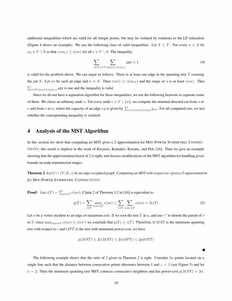
The following example shows that the ratio of 2 given in Theorem 2 is tight. Consider 2n points located on a

single line such that the distance between consecutive points alternates between 1 and ε < 1 (see Figure 5) and let

κ = 2. Then the minimum spanning tree MST connects consecutive neighbors and has power-cost p(MST ) = 2n.

10

22

22 2

2 2ε

1+ε

ε

ε(1+ )εε (1+ )ε(1+ )ε ε (1+ )ε

(b)

ε1+ε 1

1 1 1ε ε

1 1 1 1 1 1 1 1

(a)

1

ε

Figure 5: Tight example for the performance ratio of the MST algorithm (κ = 2). (a) The MST-based range assignment

needs total power 2n. (b) Optimum range assignment has total power n(1 + ε) 2 + (n − 1)ε2 + 1 → n + 1.

On the other hand, the tree T with edges connecting each other node (see Figure 5(b)) has power-cost equal p(T ) =

n(1 + ε)2 + (n − 1)ε2 + 1. When n → ∞ and ε → 0, we obtain that p(MST )/p(T ) → 2.

Our MIN-POWER SYMMETRIC CONNECTIVITY formulation assumes that node transmission ranges can be ar-

bitrary non-negative numbers. In practice node specific lower- and upper-bounds on the transmission ranges may be

required. All the algorithms in this paper (including the MST algorithm) apply to the graph version of MIN-POWER

SYMMETRIC CONNECTIVITY. Hence, they can easily handle upper-bounds on transmission ranges by assigning

infinity cost to edges that cannot be established as bidirected links due to the imposed upper-bounds.

Handling the lower-bounds on transmission ranges is not straightforward. We propose the following modification

of the MST algorithm.

1. Assign to each node the minimum allowed transmission range.

2. Compute the connected components in the graph induced by the biconnected links established by the assignment

in Step 1.

3. For each two components C and C ′, compute a connection cost which is the minimum increase in power

necessary to establish a bidirectional link between some vertex in C and some vertex in C ′.

4. Construct a complete graph G′ with the connected components as vertices and connection costs as edge costs.

5. Increase power ranges according to the MST in the graph G ′.

Theorem 3 The MST algorithm modified as above has an approximation factor of 2 for MIN-POWER SYMMETRIC

CONNECTIVITY problem with lower-bounds on transmission ranges.

11

5 k-Restricted Approach to Symmetric Min-Power Connectivity Approxi-

mation

We first give definitions of k-restricted decompositions and prove an upper bound on the power-cost of such decom-

positions. Then we will describe approximation algorithms whose approximation ratios follow from the performance

ratios of Steiner tree algorithms in graphs.

5.1 k-Restricted Decompositions

A k-restricted decomposition Q of an undirected tree T is a partition of T into subtrees T 1, T2, . . . , Tp each containing

at most k vertices such that each edge of T belongs to exactly one subtree T i. The power-cost p(Q) of Q is defined to

be the sum of the power-costs of all of its elements, i.e., p(Q) =∑

Ti∈Q p(Ti). The tight example for Theorem 5 in

Figure 7 gives examples of 3-restricted decompositions.

The following theorem and its proof are similar to the results of [13, 4] on the k-restricted Steiner ratio. Our current

theoretically best approximation algorithm does not make use of this theorem, but we use the theorem to establish the

performance ratio of more practical algorithms derived from [2, 32].

Theorem 4 For every weighted tree T and every k ≥ 1, there is a 2k-restricted decomposition Q of T such that

p(Q) ≤ (1 + 1/k)p(T ).

Proof: Without loss of generality we can assume that all edge costs are different. Let the endpoints r and s of the

heaviest edge h of T be the roots of T , which means that two subtrees of T − {h} are rooted at r and s, respectively.

Then each vertex v of T , except r and s, has a unique parent. We call the vertices adjacent to v, other than the parent

of v (if defined), the children of v. For each vertex v of T , we sort the edges connecting v to its children in increasing

order of their cost. For the most costly such edge e we define next(e) = f , where f is the edge connecting v to its

parent (if v has a parent), or f = h if v does not have a parent; for every other edge e we define next(e) = e ′, where

e′ is the next edge (in the sorted order above) connecting v to one of its children.

We now construct a rooted directed binary (with arcs going toward the root) tree B as follows. The vertices of B

are the edges of T and the root of B is h, the heaviest edge of T . The arcs of B consist of arcs (e, next(e)) for each

edge e of T . It is immediate that every vertex e = uv of B has at most two incoming arcs. Indeed, if e = rs, then

only the most costly edge of T \ {e} incident to r and the most costly edge of T \ {e} incident to s have e as a parent.

For each other edge e = uv of T , where v is the parent of u, there is at most one arc coming into e from the vertex of

B representing the most costly edge of T \ {e} incident to u, and at most one arc coming into e from the vertex of B

representing the edge of T between v and one of its children that precedes e in the sorted order above. Note that each

vertex of B has an associated cost since it represents an edge of T .

Let Bi be the set of vertices of B in distance i from the root h. There is an integer 0 ≤ l < k such that∑j | j≡l (mod k) c(Bj) ≤ 1

k c(B) = 1kc(T ), and let B = ∪j | j≡l (mod k)Bj . The removal of every edge outgoing

12

from B decomposes B into subtrees Qi corresponding to subtrees Ti of T . The number of vertices in Qi is at most

2k − 1 since Qi is a binary tree of height at most k − 1. Therefore, each T i has at most 2k vertices. We denote by Q

the 2k-restricted decomposition of T into Ti’s.

Let ei = (vi, ui) be the root of Qi (note that ei ∈ B) and, if ei = (r, s), rename vi and ui such that ui is the parent

of vi in T . By the construction of B, we have that maxu | uui∈E(Ti) c(uui) = c(ei). Then we have:

p(Ti) ≤ c(ei) +∑

v∈V (Ti)\{ui}max

(v,u)∈E(T )c(v, u).

For i = j, the sets V (Ti) \ {ui} and V (Tj) \ {uj} are disjoint. We conclude that

p(Q) =∑

i

p(Ti)

≤∑

v∈V (T )

max(v,u)∈E(T )

c(v, u) +∑

i

c(ei)

≤ p(T ) + c(B)

≤ p(T ) +1k

c(T )

≤ (1 +1k

)p(T ).

A subtree of T consisting of a pair of edges sharing a node is called a fork. So a 3-restricted decomposition Q of

T consists of forks and individual edges. The following theorem is the analogue of the Steiner tree theorem in [31],

but has a completely different proof.

Theorem 5 For every tree T , there is a 3-restricted decomposition Q of T such that p(Q) ≤ 53p(T ).

Proof: The proof proceeds in three steps. First we partition the edges of T into disjoint components using structural

information derived from power requirements. Then we construct a weighted subgraph of the line graph of each

component, which we refer to as the “consecutive” line graph. Finally, we show that the consecutive line graph of

each component has a matching exceeding a certain weight; the edges in these matchings give the forks in the desired

3-restricted decomposition of T .

To describe how we partition the edges of T (see Figure 6(a)) we need to introduce some additional notations.

Let max(u) be the maximum edge of T incident to a vertex u. 1 For each vertex u, we direct the edge max(u) away

from u. An edge uv is called root if it is directed both ways (i.e., max(u) = max(v) = uv), and called bridge if it

remains undirected (i.e., max(u) = uv and max(v) = uv). In the power-cost of T , roots are counted twice (for both

endpoints), bridges are not counted at all, and all other edges are counted exactly once. Thus, denoting by R the set of

1W.l.o.g., we assume that no two edges of T have the same cost.

13

root

bridge

e2

e4

e5

e6

(a)

v0

e3root

e1 e7root

bridge

e1

e2 e3

e4

e5

e6

e7

root

(b)

Figure 6: (a) Partitioned tree T . Each vertex has a single outgoing arc denoting its maximum incident edge, double

arcs are roots and dashed edges are bridges. (b) Consecutive line graphs for the components. Vertices represent edges

of T ; “consecutive” forks of T are represented by the solid edges, “parity” edges are dashed.

roots and by B the set of bridges, we have:

p(T ) = c(T ) + c(R) − c(B) (6)

The edges of T are partitioned as follows. First, we start with the connected components of T − B; note that each

such component contains exactly one root. Then we add each bridge b of B to one of the two adjacent components

of T − B, such that each component gets at most one bridge. A bridge assignment with this property is obtained

by selecting an arbitrary vertex v0 and assigning to each component of T − B not containing v 0 the unique adjacent

bridge on the path to v0. We denote by D the resulting partition.

A fork (e1 = uv, e2 = u′v) is called consecutive if c(e1) < c(e2) and there is no edge e∈ D incident to v such

that c(e1) < c(e) < c(e2). For each component D ∈ D, the consecutive line graph LD is defined as follows (see

Figure 6(b)):

– vertices of LD are the edges of D

– LD has “consecutive” edges connecting each consecutive forks of D, and at most two “parity” edges connecting

the root of D and the second most expensive non-root edge incident to each end of the root

– for every edge (e1, e2) of LD, w(e1, e2) = min{c(e1), c(e2)}

By construction, each edge of LD corresponds to a fork of D. Therefore, each matching X of L D corresponds to a

3-restricted decomposition of D (edges of X correspond to forks and isolated vertices correspond to isolated edges)

which we denote QX . It is easy to see that p(QX) = 2c(D) − w(X).

The theorem follows if, for each D ∈ D, we find a matching XD in LD such that

w(XD) ≥ c(D) − c(rD) + c(bD)3

(7)

where c(D) is the total cost of the edges in D, rD is the single root in D, and bD is the single bridge in D, if one

exists. Indeed,

p(⋃

D∈DQXD ) =

∑D∈D

(2c(D) − w(XD))

14

≤∑D∈D

(53c(D) +

13c(rD) − 1

3c(bD)

)

=53c(T ) +

13c(R) − 1

3c(B)

≤ 53p(T )

where the last inequality comes from (6) and the fact that c(T ) ≤ p(T ), as in the proof of Theorem 2.

By Edmonds’ theorem [19] it is sufficient to construct a fractional matching X D satisfying (7). A fractional

matching of LD is an assignment of nonnegative fractions x(e1, e2) to every edge (e1, e2) ∈ LD such that

(i) the sum of fractions assigned to the edges incident to a vertex e of L D is at most 1, and

(ii) the sum of fractions assigned to all edges with both endpoints in a set of 2k + 1 vertices of L D is at most k.

The weight of a fractional matching XD is given by

w(XD) =∑

(e,e′)∈E(D)

x(e, e′)w(e, e′)

We construct a fractional matching XD by assigning 1/3 to each consecutive edge (e1, e2) of LD. This fractional

matching satisfies (i) since each e ∈ D is incident to at most 3 consecutive edges of LD (if e is not the root rD , then it

participates to one consecutive edge of LD as e1, and to at most two edges as e2; the root participates as the heaviest

end in up to two edges). Condition (ii) follows from the fact that consecutive edges form a tree. Since every vertex e

of LD except the root participates in exactly one consecutive fork (e 1, e2) as e1, we get that the weight of X ′D is equal

to (c(D) − c(rD))/3.

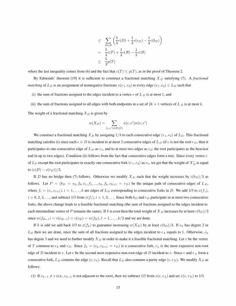
If D has no bridge then (7) follows. Otherwise we modify XD such that the weight increases by c(bD)/3 as

follows. Let P = (bD = e0, f0, e1, f1, ..., ek, fk, ek+1 = rD) be the unique path of consecutive edges of LD,

where fi = (ei, ei+1), i = 1, . . . , k are edges of LD corresponding to consecutive forks in D. We add 1/3 to x(f i),

i = 0, 2, 4, . . ., and subtract 1/3 from x(fi), i = 1, 3, . . .. Since both bD and rD participate in at most two consecutive

forks, the above change leads to a feasible fractional matching (the sum of fractions assigned to the edges incident to

each intermediate vertex of P remains the same). If k is even then the total weight of X D increases by at least c(bD)/3

since w(f2l−1) = c(e2l−1) < c(e2l) = w(f2l), l = 1, . . . , k/2 and we are done.

If k is odd we add back 1/3 to x(fk) to guarantee increasing w(XD) by at least c(bD)/3. If ek has degree 2 in

LD then we are done, since the sum of all fractions assigned to the edges incident to e k equals to 1. Otherwise, ek

has degree 3 and we need to further modify XD in order to make it a feasible fractional matching. Let v be the vertex

of T common to ek and rD . Since fk = (ek, ek+1 = rD) is a consecutive fork, ek is the most expensive non-root

edge of D incident to v. Let e be the second most expensive non-root edge of D incident to v. Since e and e k form a

consecutive fork, LD contains the edge (e, ek). Recall that LD also contains a parity edge (e, rD). We modify XD as

follows:

(1) If ek−1 = e (i.e., ek−1 is not adjacent to the root), then we subtract 1/3 from x(e, ek) and set x(e, rD) to 1/3.

15

2

1 1 1

2222

1

1

222

222

(c)

. . .

. . .

2 2 22

2 2 2

2 2 2 2

1 1 1 1

1

1 1

1 1 1

11

1

v

111

2

. . .

. . .

(b)

2

22 2

1111

2

. . .

. . .

(a)

2

1 1 1 1

2 2 2

Figure 7: (a) Tight example for Theorem 5: a single node is connected via cost-2 edges to k nodes, each of which is

in turn connected via a cost-1 edge to a leaf. The total power-cost of this tree is 2 + 2k + k = 3k + 2. (b-c) Two

minimum 3-restricted decompositions: the power-cost of (b) is 5k since each of k forks has power-cost 5; and the

power-cost of (c) is 6 k2 +2k = 5k since each of k

2 upper forks has power-cost 6 and each of k single-edge components

has power-cost 2.

(2) If ek−1 = e (i.e., ek−1 is adjacent to the root), then we subtract 1/3 from x(fk−1) and set x(e = ek−1, rD) to

1/3.

In both cases, the resulting sums of fractions assigned to the edges incident to e k, respectively to rD, are equal to 1,

and hence XD satisfies (i). In case (1), the condition (ii) is valid since edges with non-zero fraction in X D continue

to form a tree. In case (2), the condition (ii) is still valid: the graph given by the edges with non-zero fraction has only

one cycle, and therefore any set of 2k + 1 vertices of LD induces a subgraph with at most 2k + 1 edges with non-zero

fraction (each of them having fraction 1/3).

Remark: The bound of Theorem 5 is tight (see Figure 7).

5.2 Approximation Algorithms

All approximation algorithms described below have approximation ratios defined in terms of ρ k, where ρk is the

supremum, over all trees T , of the ratio of the power-cost of the minimum power-cost k-restricted decompositions to

the power-cost of T . Theorem 4 implies that ρk ≤ 1 + 1�lg k� , in particular ρ4 ≤ 3

2 . Theorem 5 together with the

example in Figure 7 imply that ρ3 = 5/3, while Theorem 2 together with the example in Figure 5 imply that ρ 2 = 2.

The following Greedy Fork-Contraction (GFC) algorithm, originally formulated for Steiner trees, is based on the

notion of gain, defined below. For a graph G, denote by mst(G) the minimum cost of a spanning tree. For a set of

vertices V ′ ⊆ V (G), we denote by G/V ′ the graph obtained after contracting V ′, i.e., collapsing all vertices of V ′

into a single vertex. Let G be obtained from G0 after contracting some subsets of vertices, H be a subtree of G0, and

VG(H) be the set of vertices of G which, seen as subsets of V (G0), intersect V (H). The gain of H with respect to G

is:

gainG(H) = 2mst(G) − 2mst(G/VG(H)) − p(H)

16

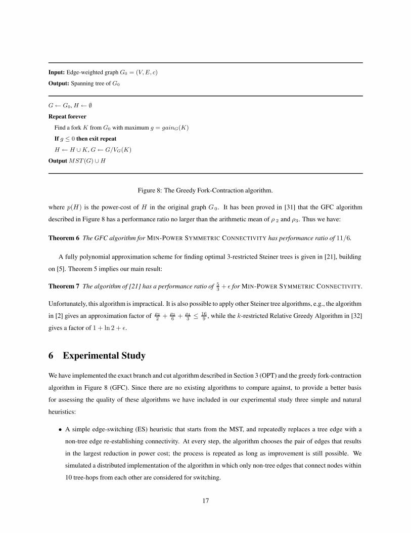
Input: Edge-weighted graph G0 = (V, E, c)

Output: Spanning tree of G0

G ← G0, H ← ∅Repeat forever

Find a fork K from G0 with maximum g = gainG(K)

If g ≤ 0 then exit repeat

H ← H ∪ K, G ← G/VG(K)

Output MST (G) ∪ H

Figure 8: The Greedy Fork-Contraction algorithm.

where p(H) is the power-cost of H in the original graph G0. It has been proved in [31] that the GFC algorithm

described in Figure 8 has a performance ratio no larger than the arithmetic mean of ρ 2 and ρ3. Thus we have:

Theorem 6 The GFC algorithm for MIN-POWER SYMMETRIC CONNECTIVITY has performance ratio of 11/6.

A fully polynomial approximation scheme for finding optimal 3-restricted Steiner trees is given in [21], building

on [5]. Theorem 5 implies our main result:

Theorem 7 The algorithm of [21] has a performance ratio of 53 + ε for MIN-POWER SYMMETRIC CONNECTIVITY.

Unfortunately, this algorithm is impractical. It is also possible to apply other Steiner tree algorithms, e.g., the algorithm

in [2] gives an approximation factor of ρ22 + ρ3

6 + ρ43 ≤ 16

9 , while the k-restricted Relative Greedy Algorithm in [32]

gives a factor of 1 + ln 2 + ε.

6 Experimental Study

We have implemented the exact branch and cut algorithm described in Section 3 (OPT) and the greedy fork-contraction

algorithm in Figure 8 (GFC). Since there are no existing algorithms to compare against, to provide a better basis

for assessing the quality of these algorithms we have included in our experimental study three simple and natural

heuristics:

• A simple edge-switching (ES) heuristic that starts from the MST, and repeatedly replaces a tree edge with a

non-tree edge re-establishing connectivity. At every step, the algorithm chooses the pair of edges that results

in the largest reduction in power cost; the process is repeated as long as improvement is still possible. We

simulated a distributed implementation of the algorithm in which only non-tree edges that connect nodes within

10 tree-hops from each other are considered for switching.

17

• A heuristic performing both edge and fork switching (EFS). At every step the algorithm chooses an edge or fork

whose addition to the tree leads to the largest reduction in power cost. Unlike GFC, forks are not contracted,

which means that an edge of an added fork can be later removed from the tree by other edge or fork switches.

• A Kruskal-like heuristic (KR) that starts with isolated nodes and iteratively adds an edge connecting two dif-

ferent components with minimum increase in power cost. A similar heuristic (called incremental search) was

studied by Chu and Nikolaidis for computing low-power MIN-POWER ASYMMETRIC BROADCAST trees in a

mobile environment [7].

We included in our comparison faster versions of OPT and GFC, OPT-D and GFC-D, which speed-up the computation

by working on the Delaunay graph (see, e.g., [12]) defined by the nodes instead of the complete graph. We also

implemented a faster version of EFS, EFS-D, in which only forks consisting of Delaunay edges (but still all non-tree

edges) are considered as switching candidates.

Note that, by Theorem 2, both ES and EFS produce solutions within a factor of 2 of optimum since they improve

upon an MST for the nodes. A performance of ratio of 2 can be proven for KR as well. Define a new cost function

c(e) as follows: if e is not picked by the KR, then c(e) = c(e), else c(e) is the increase in power cost used by KR

to pick e. It can be proven that the minimum spanning tree in (V, E, c) is the same as the tree picked by KR in G,

and since for every e ∈ E we have c(e) ≤ c(e), the optimum solution in (V, E, c) has power at most the optimum

power in G. An example showing that the performance ratio of 2 is tight for KR in the graph model is given below;

the exact performance ratio in E 2 is not known. The q + 3 vertices are v0, v1, v2, . . . , vq+2, and the edges have cost:

for i = 0, 1, . . . , q, c(vivq+1) = 1 and c(vivq+2) = 2 − 12i − ε, and c(vq+1vq+2) = ε. KR builds a star centered at

vq+2 with a power-cost of about 2q, while the optimum solution is a star centered at v q+1 with a power-cost of about

q.

All algorithms were implemented in C++, including the branch and bound algorithm whose implementation is

built on SCIL [25]. The heuristics were compiled using gpp with -O2 optimization, and run on an AMD Duron

600MHz PC. The experiments were run on randomly generated testcases. For each instance size n between 10 and

100, in increments of 5, 50 different instances were generated by choosing n points uniformly at random from a grid

of size 10, 000× 10, 000.

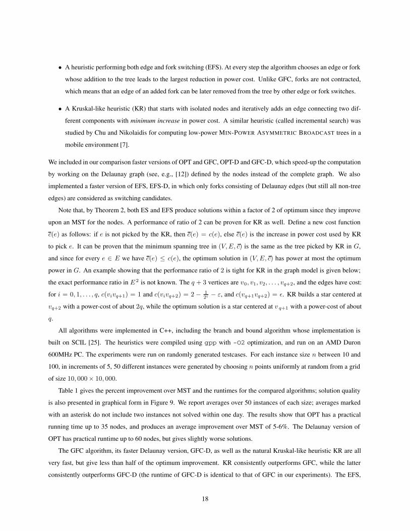
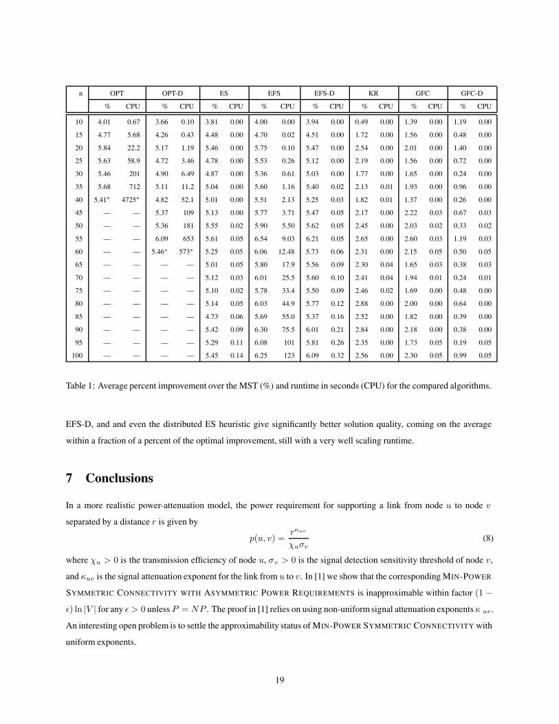
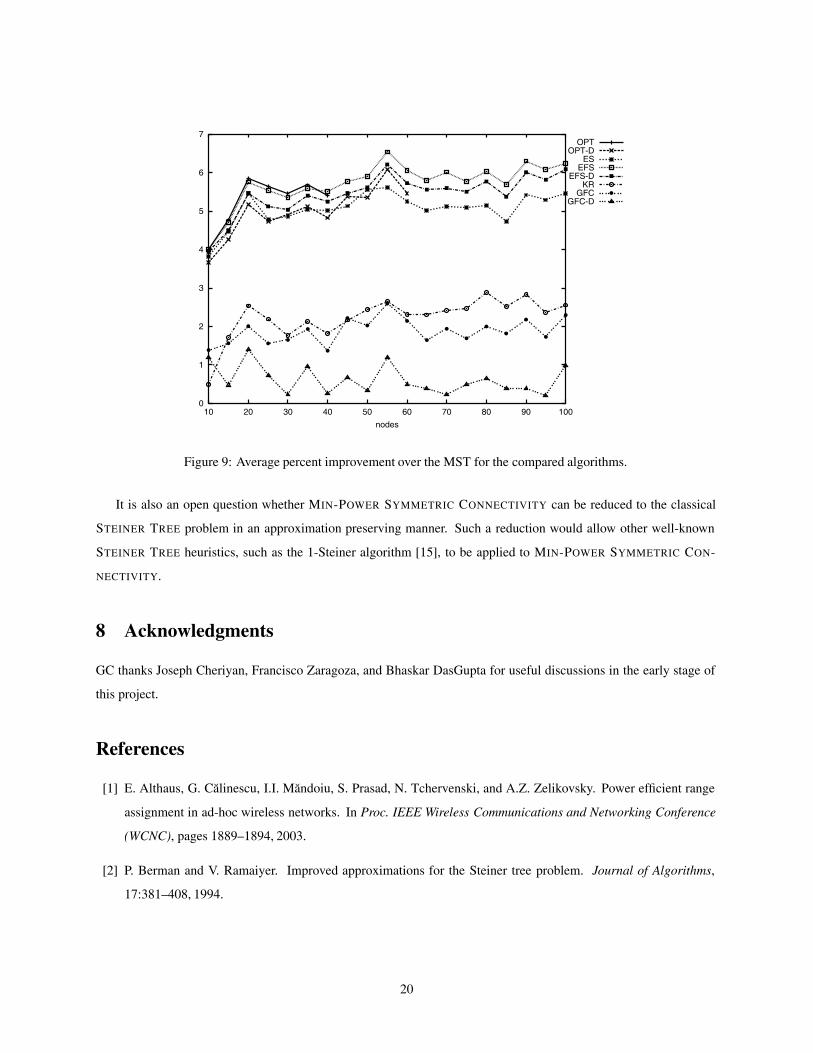
Table 1 gives the percent improvement over MST and the runtimes for the compared algorithms; solution quality

is also presented in graphical form in Figure 9. We report averages over 50 instances of each size; averages marked

with an asterisk do not include two instances not solved within one day. The results show that OPT has a practical

running time up to 35 nodes, and produces an average improvement over MST of 5-6%. The Delaunay version of

OPT has practical runtime up to 60 nodes, but gives slightly worse solutions.

The GFC algorithm, its faster Delaunay version, GFC-D, as well as the natural Kruskal-like heuristic KR are all

very fast, but give less than half of the optimum improvement. KR consistently outperforms GFC, while the latter

consistently outperforms GFC-D (the runtime of GFC-D is identical to that of GFC in our experiments). The EFS,

18

n OPT OPT-D ES EFS EFS-D KR GFC GFC-D

% CPU % CPU % CPU % CPU % CPU % CPU % CPU % CPU

10 4.01 0.67 3.66 0.10 3.81 0.00 4.00 0.00 3.94 0.00 0.49 0.00 1.39 0.00 1.19 0.00

15 4.77 5.68 4.26 0.43 4.48 0.00 4.70 0.02 4.51 0.00 1.72 0.00 1.56 0.00 0.48 0.00

20 5.84 22.2 5.17 1.19 5.46 0.00 5.75 0.10 5.47 0.00 2.54 0.00 2.01 0.00 1.40 0.00

25 5.63 58.9 4.72 3.46 4.78 0.00 5.53 0.26 5.12 0.00 2.19 0.00 1.56 0.00 0.72 0.00

30 5.46 201 4.90 6.49 4.87 0.00 5.36 0.61 5.03 0.00 1.77 0.00 1.65 0.00 0.24 0.00

35 5.68 712 5.11 11.2 5.04 0.00 5.60 1.16 5.40 0.02 2.13 0.01 1.93 0.00 0.96 0.00

40 5.41∗ 4725∗ 4.82 52.1 5.01 0.00 5.51 2.13 5.25 0.03 1.82 0.01 1.37 0.00 0.26 0.00

45 — — 5.37 109 5.13 0.00 5.77 3.71 5.47 0.05 2.17 0.00 2.22 0.03 0.67 0.03

50 — — 5.36 181 5.55 0.02 5.90 5.50 5.62 0.05 2.45 0.00 2.03 0.02 0.33 0.02

55 — — 6.09 653 5.61 0.05 6.54 9.03 6.21 0.05 2.65 0.00 2.60 0.03 1.19 0.03

60 — — 5.46∗ 573∗ 5.25 0.05 6.06 12.48 5.73 0.06 2.31 0.00 2.15 0.05 0.50 0.05

65 — — — — 5.01 0.05 5.80 17.9 5.56 0.09 2.30 0.04 1.65 0.03 0.38 0.03

70 — — — — 5.12 0.03 6.01 25.5 5.60 0.10 2.41 0.04 1.94 0.01 0.24 0.01

75 — — — — 5.10 0.02 5.78 33.4 5.50 0.09 2.46 0.02 1.69 0.00 0.48 0.00

80 — — — — 5.14 0.05 6.03 44.9 5.77 0.12 2.88 0.00 2.00 0.00 0.64 0.00

85 — — — — 4.73 0.06 5.69 55.0 5.37 0.16 2.52 0.00 1.82 0.00 0.39 0.00

90 — — — — 5.42 0.09 6.30 75.5 6.01 0.21 2.84 0.00 2.18 0.00 0.38 0.00

95 — — — — 5.29 0.11 6.08 101 5.81 0.26 2.35 0.00 1.73 0.05 0.19 0.05

100 — — — — 5.45 0.14 6.25 123 6.09 0.32 2.56 0.00 2.30 0.05 0.99 0.05

Table 1: Average percent improvement over the MST (%) and runtime in seconds (CPU) for the compared algorithms.

EFS-D, and and even the distributed ES heuristic give significantly better solution quality, coming on the average

within a fraction of a percent of the optimal improvement, still with a very well scaling runtime.

7 Conclusions

In a more realistic power-attenuation model, the power requirement for supporting a link from node u to node v

separated by a distance r is given by

p(u, v) =rκuv

χuσv(8)

where χu > 0 is the transmission efficiency of node u, σv > 0 is the signal detection sensitivity threshold of node v,

and κuv is the signal attenuation exponent for the link from u to v. In [1] we show that the corresponding MIN-POWER

SYMMETRIC CONNECTIVITY WITH ASYMMETRIC POWER REQUIREMENTS is inapproximable within factor (1 −ε) ln |V | for any ε > 0 unless P = NP . The proof in [1] relies on using non-uniform signal attenuation exponents κ uv .

An interesting open problem is to settle the approximability status of MIN-POWER SYMMETRIC CONNECTIVITY with

uniform exponents.

19

0

1

2

3

4

5

6

7

10 20 30 40 50 60 70 80 90 100

nodes

OPTOPT-D

ESEFS

EFS-DKR

GFCGFC-D

Figure 9: Average percent improvement over the MST for the compared algorithms.

It is also an open question whether MIN-POWER SYMMETRIC CONNECTIVITY can be reduced to the classical

STEINER TREE problem in an approximation preserving manner. Such a reduction would allow other well-known

STEINER TREE heuristics, such as the 1-Steiner algorithm [15], to be applied to MIN-POWER SYMMETRIC CON-

NECTIVITY.

8 Acknowledgments

GC thanks Joseph Cheriyan, Francisco Zaragoza, and Bhaskar DasGupta for useful discussions in the early stage of

this project.

References

[1] E. Althaus, G. Calinescu, I.I. Mandoiu, S. Prasad, N. Tchervenski, and A.Z. Zelikovsky. Power efficient range

assignment in ad-hoc wireless networks. In Proc. IEEE Wireless Communications and Networking Conference

(WCNC), pages 1889–1894, 2003.

[2] P. Berman and V. Ramaiyer. Improved approximations for the Steiner tree problem. Journal of Algorithms,

17:381–408, 1994.

20

[3] D.M. Blough, M. Leoncini, G. Resta, and P. Santi. On the symmetric range assignment problem in wireless ad

hoc networks. In 2nd IFIP International Conference on Theoretical Computer Science (TCS 2002), pages 71–82.

Kluwer Academic Publishers, 2002.

[4] A. Borchers and D.-Z. Du. The k-Steiner ratio in graphs. SIAM Journal on Computing, 26:857–869, 1997.

[5] P.M. Camerini, G. Galbiati, and F. Maffioli. Random pseudo-polynomial algorithms for exact matroid problems.

Journal of Algorithms, 13:258–273, 1992.

[6] E.-A. Choukhmane. Une heuristique pour le probleme de l’arbre de Steiner. RAIRO Rech. Oper., 12:207–212,

1978.

[7] T. Chu and I. Nikolaidis. Energy efficient broadcast in mobile ad hoc networks. In Proc. AD-HOC Networks and

Wireless, 2002.

[8] A.E.F. Clementi, P. Crescenzi, P. Penna, G. Rossi, and P. Vocca. On the complexity of computing minimum

energy consumption broadcast subgraphs. In Symposium on Theoretical Aspects of Computer Science, pages

121–131, 2001.

[9] A.E.F. Clementi, P. Penna, and R. Silvestri. On the power assignment problem in radio networks. Electronic

Colloquium on Computational Complexity (ECCC), (054), 2000.

[10] T.H. Cormen, C.E. Leiserson, and R.L. Rivest. Introduction to algorithms (2nd ed.). MIT Press, Cambridge,

Massachusetts, 2001.

[11] G. Calinescu, I.I. Mandoiu, and A.Z. Zelikovsky. Symmetric connectivity with minimum power consumption

in radio networks. In 2nd IFIP International Conference on Theoretical Computer Science (TCS 2002), pages

119–130. Kluwer Academic Publishers, 2002.

[12] M. de Berg, M. van Kreveld, M. Overmars, and O. Schwarzkopf. Computational Geometry - Algorithms and

Applications. Springer Verlag, Berlin, 1997.

[13] D.-Z. Du, Y.-J. Zhang, and Q. Feng. On better heuristic for Euclidean Steiner minimum trees. In Proc. 32nd

Annual IEEE Symposium on Foundations of Computer Science, pages 431–439, 1991.

[14] S. Guha and S. Khuller. Approximation algorithms for connected dominating sets. Algorithmica, 20:374–387,

1998.

[15] A. B. Kahng and G. Robins. A new class of iterative Steiner tree heuristics with good performance. IEEE

Transactions on Computer-Aided Design, 11:893–902, 1992.

[16] L.M. Kirousis, E. Kranakis, D. Krizanc, and A. Pelc. Power consumption in packet radio networks. Theoretical

Computer Science, 243:289–305, 2000.

21

[17] L. Kou, G. Markowsky, and L. Berman. A fast algorithm for Steiner trees. Acta Informatica, 15:141–145, 1981.

[18] E. Lloyd, R. Liu, M. Marathe, R. Ramanathan, and S.S. Ravi. Algorithmic aspects of topology control problems

for ad hoc networks. In Proc. ACM MobiHoc, pages 123–134, 2002.

[19] L. Lovasz and M.D. Plummer. Matching theory. North-Holland, Amsterdam–New York, 1986.

[20] M. Padberg and L. Wolsey. Trees and cuts. Anals of Discrete Mathematics, 17:511–517, 1983.

[21] H.J. Promel and A. Steger. A new approximation algorithm for the Steiner tree problem with performance ratio

5/3. Journal of Algorithms, 36:89–101, 2000.

[22] R. Ramanathan and R. Hain. Topology control of multihop wireless networks using transmit power adjustment.

In Proc. IEEE INFOCOM, pages 404–413, 2000.

[23] T.S. Rappaport. Wireless Communications: Principles and Practices. Prentice Hall, 1996.

[24] G. Robins and A. Zelikovsky. Improved Steiner tree approximation in graphs. In Proceedings of the 11th

ACM-SIAM Annual Symposium on Discrete Algorithms, pages 770–779, 2000.

[25] SCIL–Symbolic Constraints for Integer Linear programming. www.mpi-sb.mpg.de/SCIL.

[26] S. Singh, C.S. Raghavendra, and J. Stepanek. Power-aware broadcasting in mobile ad hoc networks. In Proceed-

ings of IEEE PIMRC, 1999.

[27] A.S. Tanembaum. Computer Networks (3rd edition). Prentice Hall, 1996.

[28] Mikkel Thorup. Undirected single-source shortest paths with positive integer weights in linear time. Journal of

the ACM, 46:362–394, 1999.

[29] P.-J. Wan, G. Calinescu, X.-Y. Li, and O. Frieder. Minimum energy broadcast routing in static ad hoc wireless

networks. In Proc. IEEE INFOCOM, pages 1162–1171, 2001.

[30] J.E. Wieselthier, G.D. Nguyen, and A. Ephremides. On the construction of energy-efficient broadcast and multi-

cast trees in wireless networks. In Proc. IEEE INFOCOM, pages 585–594, 2000.

[31] A. Zelikovsky. An 11/6-approximation algorithm for the network Steiner problem. Algorithmica, 9:463–470,

1993.

[32] A. Zelikovsky. Better approximation bounds for the network and Euclidean Steiner tree problems. Technical

Report CS-96-06, Department of Computer Science, University of Virginia, 1996.

22

Author biographies

Ernst Althaus received the M.S. degree in 1998 and the Ph.D. degree in 2001, both in Computer Science, from the

Universitat des Saarlandes. He worked as a postdoctoral researcher at the International Computer Science Institute

in Berkeley and at the Max-Planck-Institut fur Informatik in Saarbrucken. Ernst Althaus is now the head of an inde-

pendent research group on “optimization in bioinformatics” at the Laboratoire Lorrain de Recherche en Informatique

et ses Applications (LORIA), Nancy. His research interests include combinatorial optimization, bioinformatics, and

algorithms.

E-mail: althaus@mpi-sb.mpg.de.

Gruia Calinescu is an Assistant Professor of Computer Science at the Illinois Institute of Technology. He has a

Diploma from University of Bucharest and a PhD from Georgia Institute of Technology. His research interests are in

the area of algorithms.

E-mail: calinesc@cs.iit.edu.

Ion I. Mandoiu received the M.S. degree from Bucharest University in 1992 and the Ph.D. degree from Georgia

Institute of Technology in 2000, both in Computer Science. He is now an Assistant Professor with the Computer

Science and Engineering Department at the University of Connecticut. His research focuses on the design and analysis

of exact and approximation algorithms for NP-hard optimization problems, particularly in the areas of VLSI computer

aided design, bioinformatics, and ad-hoc wireless notworks. He authored over 40 refereed scientific publications in

these areas, including a best paper at the joint Asia-South Pacific Design Automation/VLSI Design Conferences.

E-mail: ion@engr.uconn.edu.

Sushil K. Prasad received his B. Tech. in Computer Science and Engineering from Indian Institute of Technology,

Kharagpur, in 1985, M.S. in Computer Science from Washington State University, Pullman, in 1986, and Ph.D. in

Computer Science from University of Central Florida, Orlando, in 1990. Since 1990, he has been a Professor of

Computer Science at Georgia State University (GSU), Atlanta. Currently, as P.I. of the Yamacraw/GEDC Distributed,

Mobile and Embedded Systems research contracts, he is leading a GSU team of seven faculty and 20 Ph.D./M.S.

students on developing System on Mobile Devices (SyD) middleware for collaborative computing over heterogeneous

mobile devices and data sources. Prasad has carried out theoretical as well as experimental research in parallel and

distributed computing, with over 55 publications, and made 3 utility patent applications and over a dozen provisional

patent applications. His current research interests are Parallel Algorithms and Data Structures, Parallel Discrete Event

Simulation, Web-based Distributed and Collaborative Computing, and Middlewares and Collaborative Applications

for Handheld Devices.

E-mail: sprasad@cs.gsu.edu.

Nickolay Tchervenski received his B.S. in Computer Engineering with highest honors from Illinois Institute of Tech-

23

nology in 2004. At IIT, Nickolay was advised by Prof. Calinescu. In Fall 2004, Nickolay joined the Database Research

Group at University of Waterloo where he is doing his Masters Degree in Computer Science. World finalist at the 28th

ACM International Collegiate Programming Contest in Prague, Nickolay’s research interests are in algorithms and

large databases.

E-mail: tchenic@iit.edu.

Alexander Zelikovsky received the Ph.D. degree in Computer Science from the Institute of Mathematics of the Be-

lorussian Academy of Sciences in Minsk (Belarus) in 1989 and worked at the Institute of Mathematics in Kishinev

(Moldova) (1989-1995). Between 1992 and 1995 he visited Bonn University and the Institut fur Informatik in Saar-

brueken (Germany). Dr. Zelikovsky was a Research Scientist at University of Virginia (1995-1997) and a Postdoctoral

Scholar at UCLA (1997-1998). He is an Associate Professor at Computer Science Department of Georgia State Uni-

versity which he joined in 1999. He is the author of more than 90 refereed publications. Dr. Zelikovsky’s research

interests include VLSI physical layout design, ad-hoc wireless networks, discrete and approximation algorithms, com-

binatorial optimization, and computational biology.

E-mail: alexz@cs.gsu.edu

24