Embed Size (px)
DESCRIPTION
Power 14 Goodness of Fit & Contingency Tables. Outline. I. Parting Shots On the Linear Probability Model II. Goodness of Fit & Chi Square III.Contingency Tables. The Vision Thing. Discriminating BetweenTwo Populations Decision Theory and the Regression Line. education. Players. Mean - PowerPoint PPT Presentation
Citation preview

11
Power 14Goodness of Fit
& Contingency Tables
22
Outline
I. Parting Shots On the Linear Probability I. Parting Shots On the Linear Probability ModelModel
II. Goodness of Fit & Chi SquareII. Goodness of Fit & Chi Square III.Contingency TablesIII.Contingency Tables
33
The Vision Thing
Discriminating BetweenTwo PopulationsDiscriminating BetweenTwo Populations Decision Theory and the Regression LineDecision Theory and the Regression Line
44
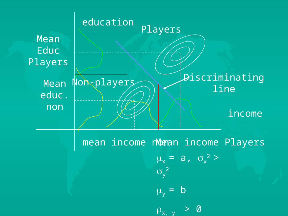
income
education
x = a, x2 > y
2
y = b
x, y > 0
mean income non
Meaneduc.non
MeanEduc
Players
Mean income Players
Players
Non-players Discriminatingline
55
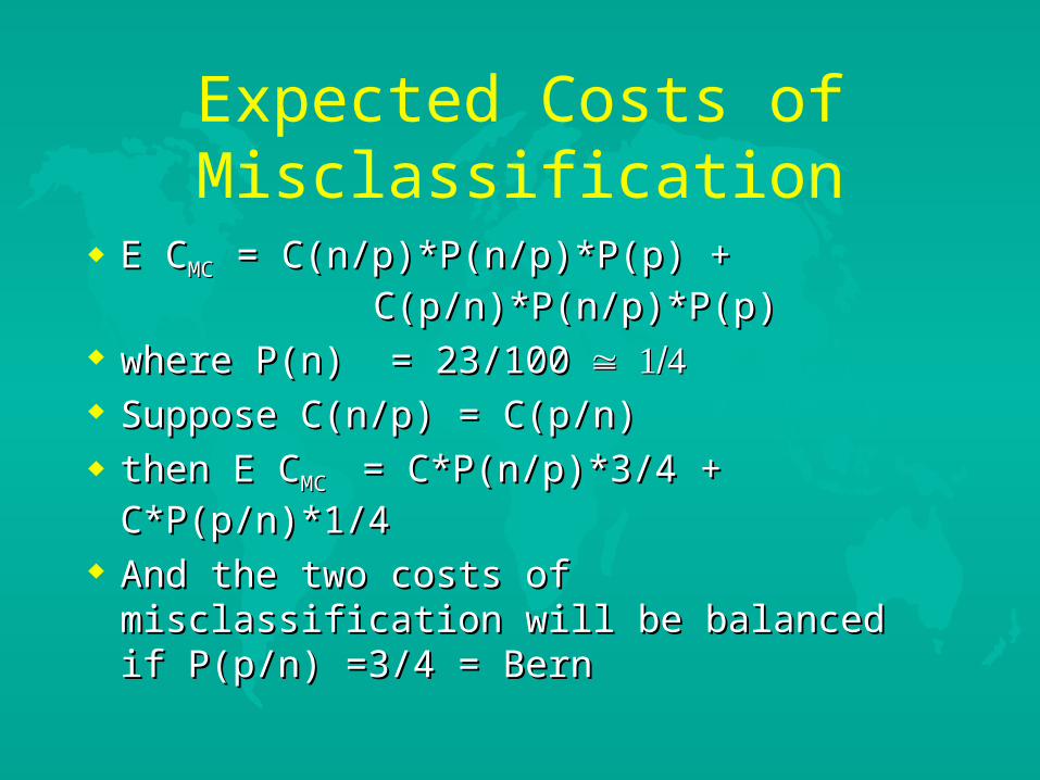
Expected Costs of Misclassification
E CE CMCMC = C(n/p)*P(n/p)*P(p) + = C(n/p)*P(n/p)*P(p) +
C(p/n)*P(n/p)*P(p)C(p/n)*P(n/p)*P(p) where P(n) = 23/100where P(n) = 23/100 Suppose C(n/p) = C(p/n)Suppose C(n/p) = C(p/n) then E Cthen E CMC MC = C*P(n/p)*3/4 + C*P(p/n)*1/4 = C*P(n/p)*3/4 + C*P(p/n)*1/4
And the two costs of misclassification will And the two costs of misclassification will be balanced if P(p/n) =3/4 = Bernbe balanced if P(p/n) =3/4 = Bern
66
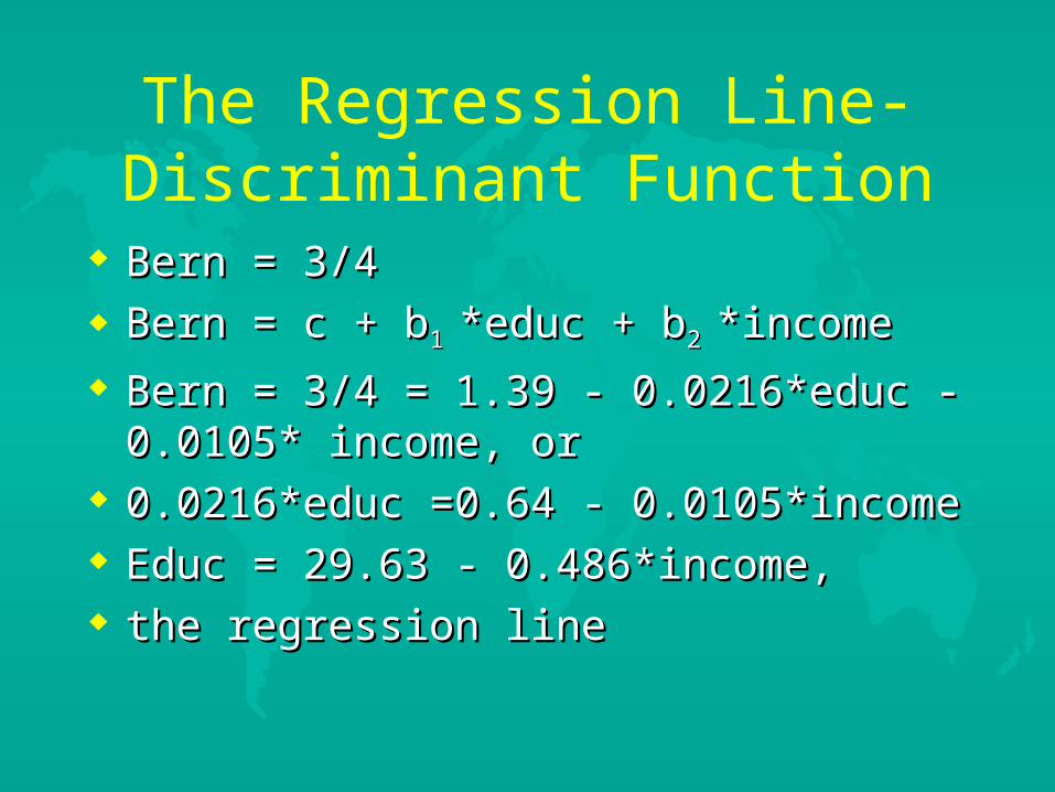
The Regression Line-Discriminant Function
Bern = 3/4Bern = 3/4 Bern = c + bBern = c + b1 1 *educ + b*educ + b2 2 *income*income
Bern = 3/4 = 1.39 - 0.0216*educ -0.0105* Bern = 3/4 = 1.39 - 0.0216*educ -0.0105* income, or income, or
0.0216*educ =0.64 - 0.0105*income0.0216*educ =0.64 - 0.0105*income Educ = 29.63 - 0.486*income, Educ = 29.63 - 0.486*income, the regression linethe regression line
77
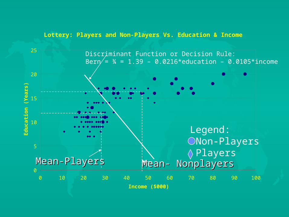
Lottery: Players and Non-Players Vs. Education & Income
0
5
10
15
20
25
0 10 20 30 40 50 60 70 80 90 100
Income ($000)
Ed
uca
tio
n (
Yea
rs)
Discriminant Function or Decision Rule:Bern = ¾ = 1.39 – 0.0216*education – 0.0105*income
Legend: Non-Players Players
Mean- NonplayersMean- NonplayersMean-PlayersMean-Players
88
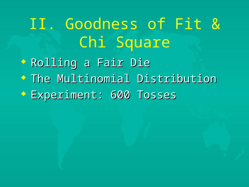
II. Goodness of Fit & Chi Square
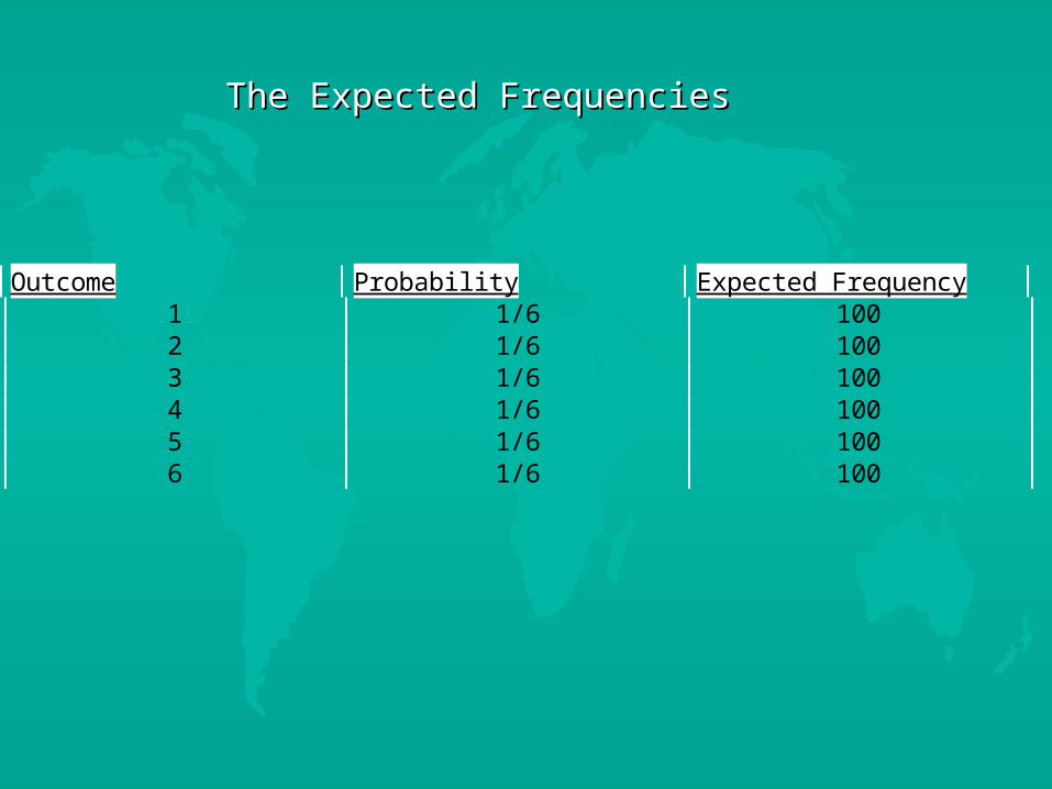
Rolling a Fair DieRolling a Fair Die The Multinomial DistributionThe Multinomial Distribution Experiment: 600 TossesExperiment: 600 Tosses
99
Outcome Probability Expected Frequency1 1/6 1002 1/6 1003 1/6 1004 1/6 1005 1/6 1006 1/6 100
The Expected Frequencies The Expected Frequencies
1010
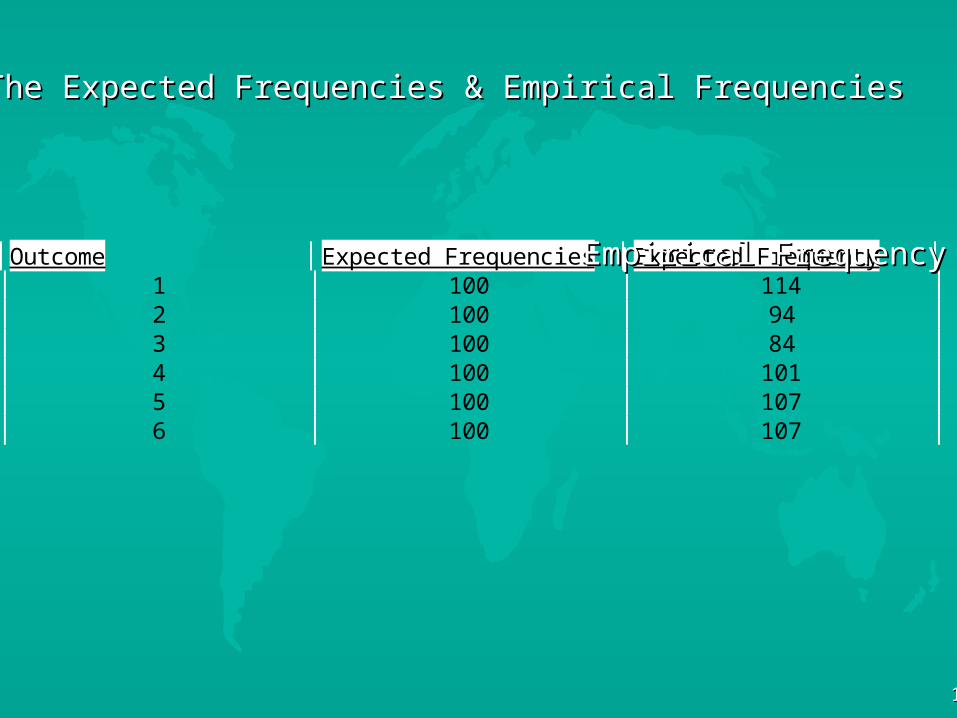
Outcome Expected Frequencies Expected Frequency1 100 1142 100 943 100 844 100 1015 100 1076 100 107
The Expected Frequencies & Empirical FrequenciesThe Expected Frequencies & Empirical Frequencies
Empirical FrequencyEmpirical Frequency
1111
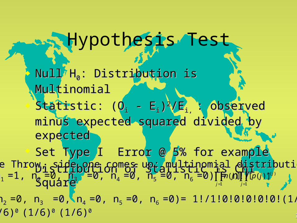
Hypothesis Test
Null HNull H00: Distribution is Multinomial: Distribution is Multinomial
Statistic: (OStatistic: (Oii - E - Eii))22/E/Ei, i, : observed minus : observed minus
expected squared divided by expectedexpected squared divided by expected Set Type I Error @ 5% for exampleSet Type I Error @ 5% for example Distribution of Statistic is Chi SquareDistribution of Statistic is Chi Square
P(nP(n1 1 =1, n=1, n2 2 =0, nn3 3 =0, n =0, n4 4 =0, n=0, n5 5 =0, n=0, n6 6 =0) = n!/=0) = n!/
n
j
jnn
j
jpjn1
)(
1
)]([])(
P(nP(n1 1 =1, n=1, n2 2 =0, nn3 3 =0, n =0, n4 4 =0, n=0, n5 5 =0, n=0, n6 6 =0)= 1!/1!0!0!0!0!0!(1/6)=0)= 1!/1!0!0!0!0!0!(1/6)11(1/6)(1/6)00
(1/6)(1/6)0 0 (1/6)(1/6)0 0 (1/6)(1/6)0 0 (1/6)(1/6)00
One Throw, side one comes up: multinomial distributionOne Throw, side one comes up: multinomial distribution
1212
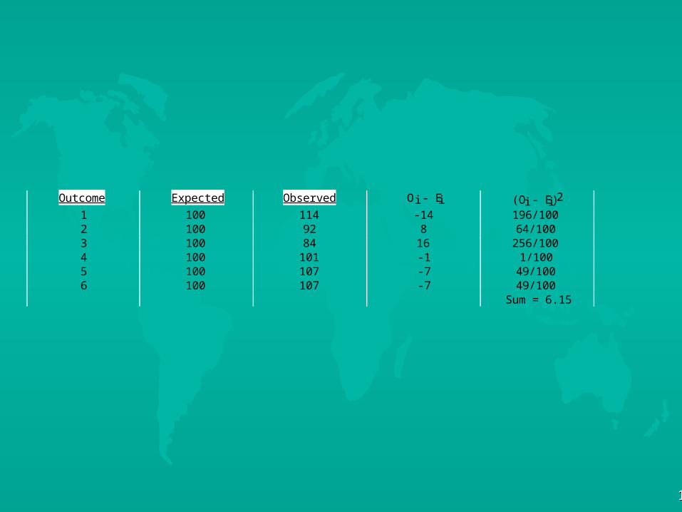
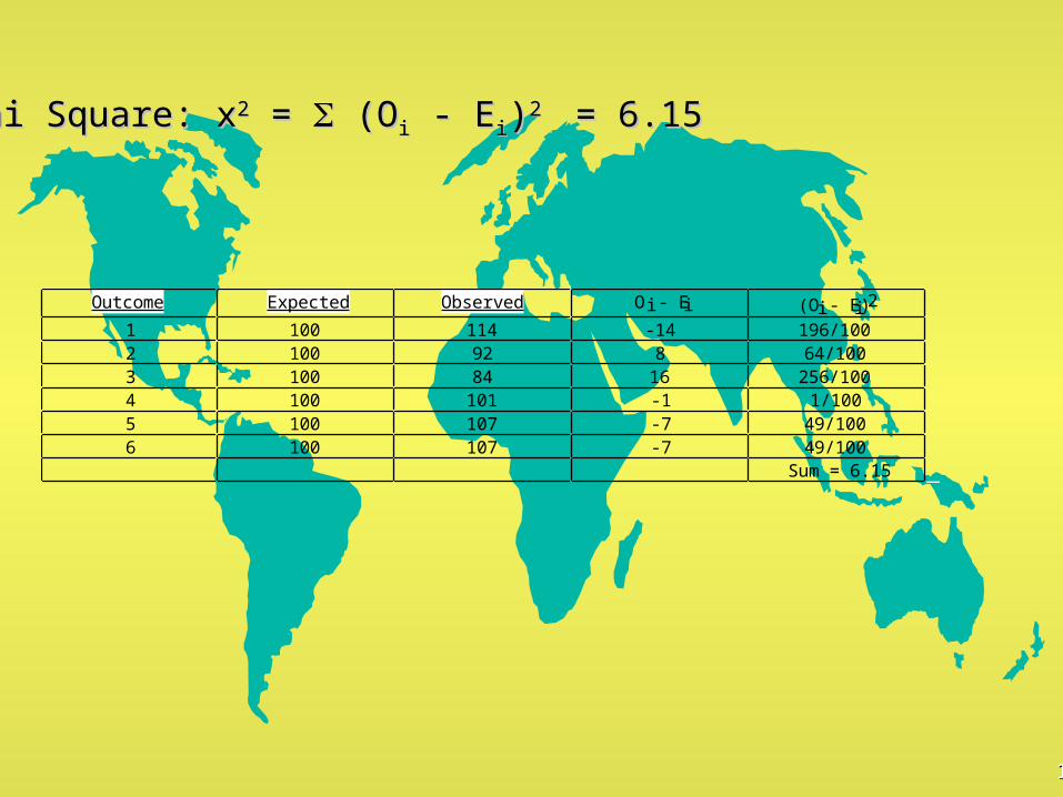
Outcome Expected Observed Oi - E i (Oi - E i)2
1 100 114 -14 196/1002 100 92 8 64/1003 100 84 16 256/1004 100 101 -1 1/1005 100 107 -7 49/1006 100 107 -7 49/100
Sum = 6.15
1313
Outcome Expected Observed Oi - E i (Oi - E i)2
1 100 114 -14 196/1002 100 92 8 64/1003 100 84 16 256/1004 100 101 -1 1/1005 100 107 -7 49/1006 100 107 -7 49/100
Sum = 6.15
Chi Square: xChi Square: x22 = = (O (Oii - E - Eii))2 2 = 6.15 = 6.15
0.00
0.05
0.10
0.15
0.20
0 5 10 15
CHI
DE
NS
ITY
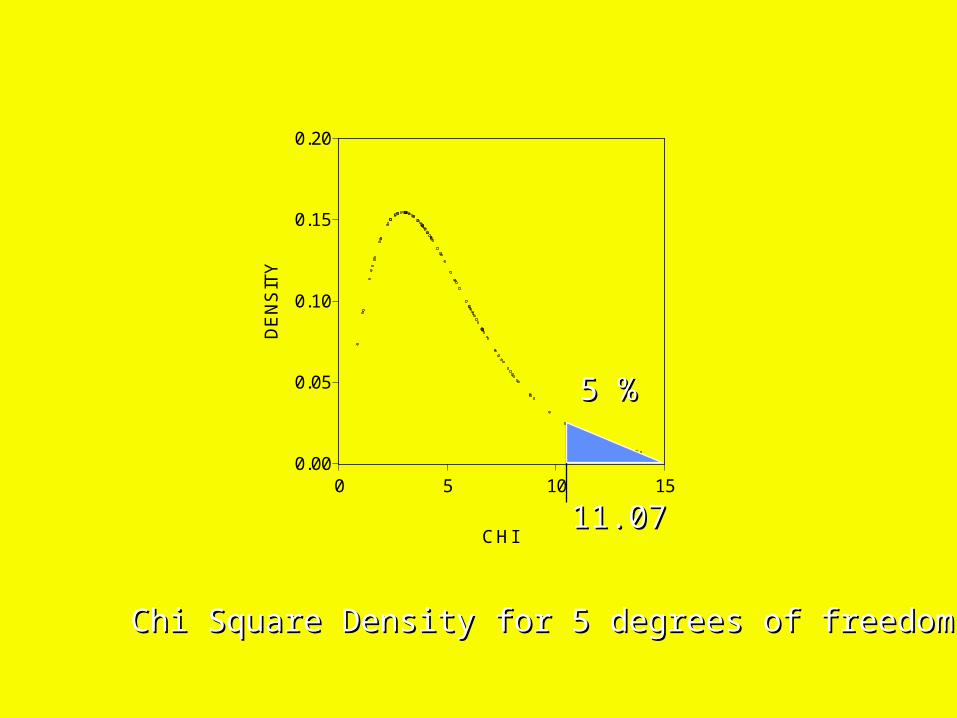
Chi Square Density for 5 degrees of freedomChi Square Density for 5 degrees of freedom
11.0711.07
5 %5 %
1515
Contingency Table Analysis
Tests for Association Vs. Independence For Tests for Association Vs. Independence For Qualitative VariablesQualitative Variables
1616
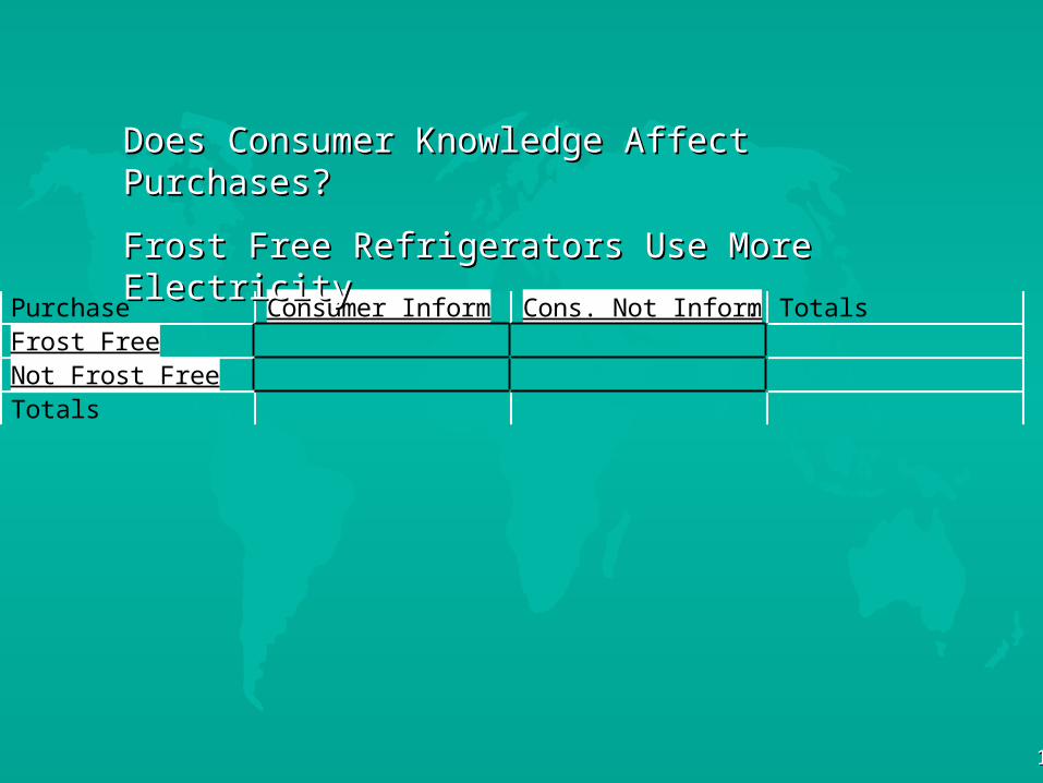
Purchase Consumer Inform Cons. Not Inform . TotalsFrost FreeNot Frost FreeTotals
Does Consumer Knowledge Affect Purchases?Does Consumer Knowledge Affect Purchases?
Frost Free Refrigerators Use More ElectricityFrost Free Refrigerators Use More Electricity
1717
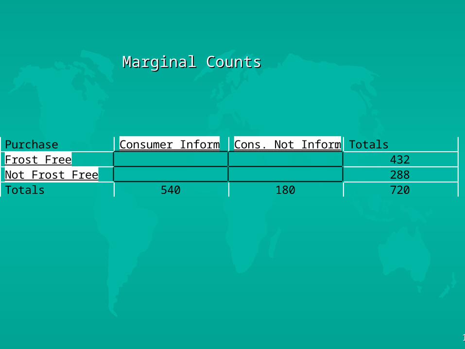
Purchase Consumer Inform Cons. Not Inform . TotalsFrost Free 432Not Frost Free 288Totals 540 180 720
Marginal CountsMarginal Counts
1818
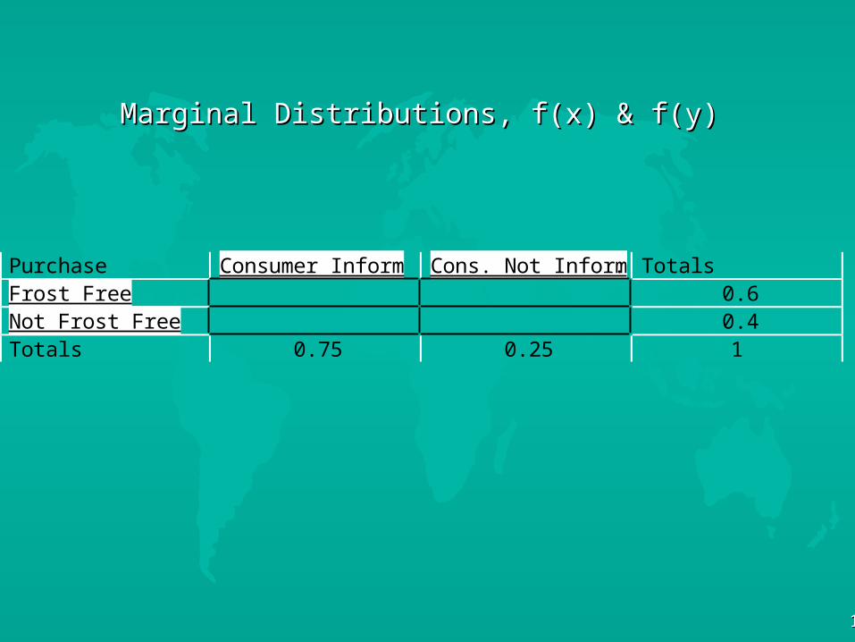
Purchase Consumer Inform Cons. Not Inform . TotalsFrost Free 0.6Not Frost Free 0.4Totals 0.75 0.25 1
Marginal Distributions, f(x) & f(y)Marginal Distributions, f(x) & f(y)
1919
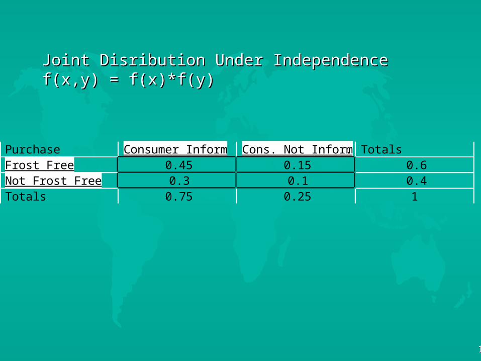
Purchase Consumer Inform Cons. Not Inform . TotalsFrost Free 0.45 0.15 0.6Not Frost Free 0.3 0.1 0.4Totals 0.75 0.25 1
Joint Disribution Under IndependenceJoint Disribution Under Independencef(x,y) = f(x)*f(y)f(x,y) = f(x)*f(y)
2020
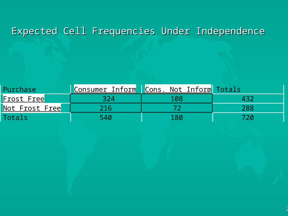
Purchase Consumer Inform Cons. Not Inform . TotalsFrost Free 324 108 432Not Frost Free 216 72 288Totals 540 180 720
Expected Cell Frequencies Under IndependenceExpected Cell Frequencies Under Independence
2121
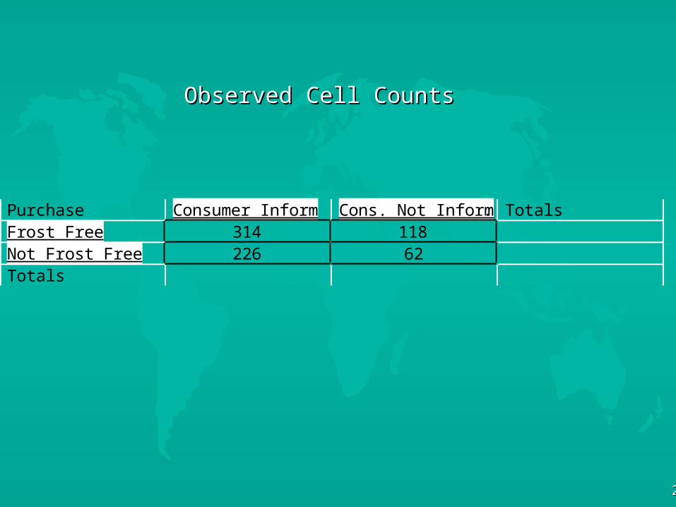
Purchase Consumer Inform Cons. Not Inform . TotalsFrost Free 314 118Not Frost Free 226 62Totals
Observed Cell CountsObserved Cell Counts
2222
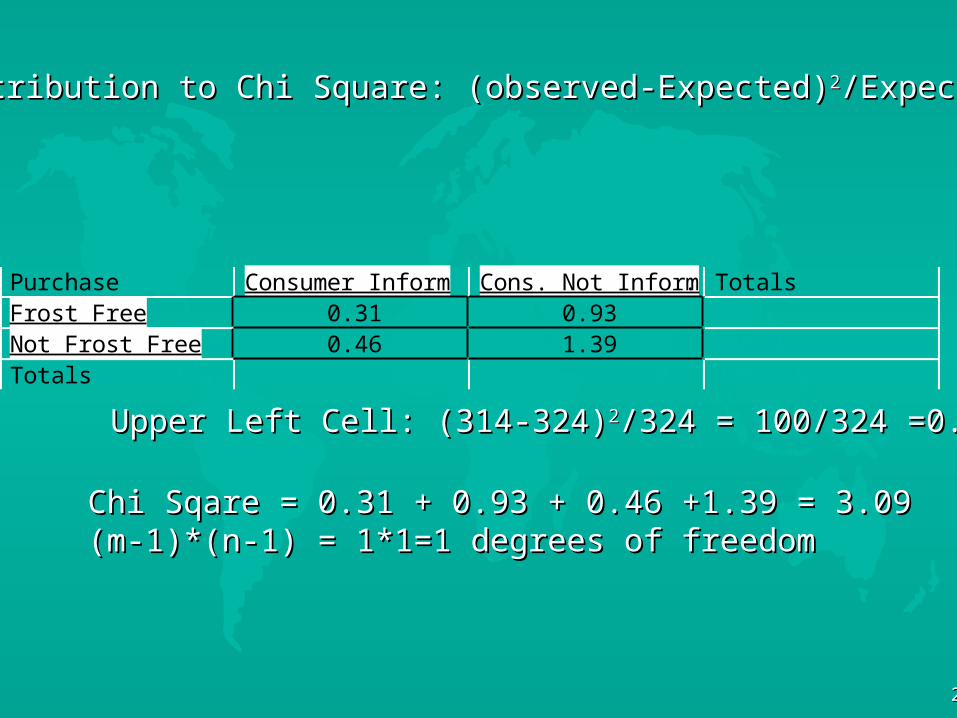
Purchase Consumer Inform Cons. Not Inform . TotalsFrost Free 0.31 0.93Not Frost Free 0.46 1.39Totals
Contribution to Chi Square: (observed-Expected)Contribution to Chi Square: (observed-Expected)22/Expected/Expected
Chi Sqare = 0.31 + 0.93 + 0.46 +1.39 = 3.09Chi Sqare = 0.31 + 0.93 + 0.46 +1.39 = 3.09(m-1)*(n-1) = 1*1=1 degrees of freedom (m-1)*(n-1) = 1*1=1 degrees of freedom
Upper Left Cell: (314-324)Upper Left Cell: (314-324)22/324 = 100/324 =0.31/324 = 100/324 =0.31
0.0
0.2
0.4
0.6
0.8
1.0
0 2 4 6 8 10 12 14
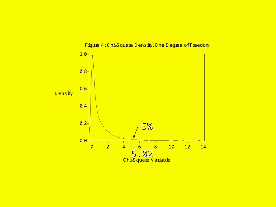
Chi-Square Variable
Figure 4: Chi-Square Density, One Degree of Freedom
Density
5%5%
5.025.02
2424
Using Goodness of Fit to Choose Between Competing
Proabaility Models Men on base when a home run is hitMen on base when a home run is hit
2525
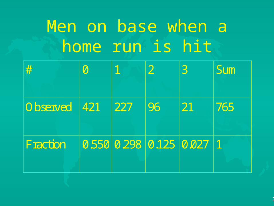
Men on base when a home run is hit
# 0 1 2 3 Sum
Observed 421 227 96 21 765
Fraction 0.550 0.298 0.125 0.027 1

2626
Conjecture
Distribution is binomialDistribution is binomial
2727
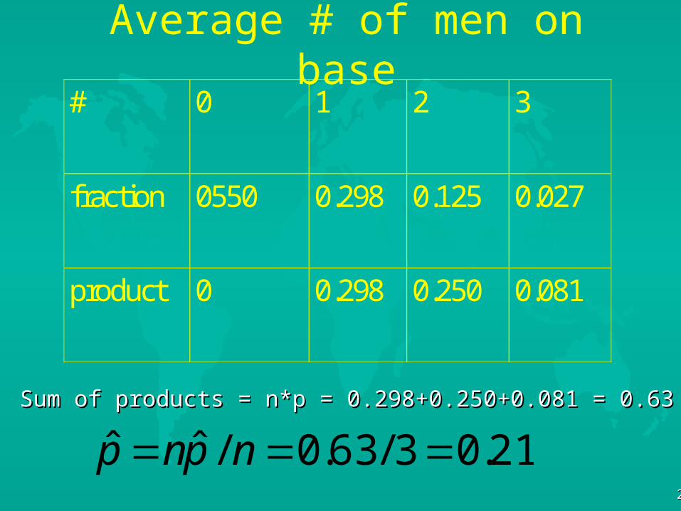
Average # of men on base# 0 1 2 3
fraction 0550 0.298 0.125 0.027
product 0 0.298 0.250 0.081
Sum of products = n*p = 0.298+0.250+0.081 = 0.63Sum of products = n*p = 0.298+0.250+0.081 = 0.63
21.03/63.0/ˆˆ npnp
2828
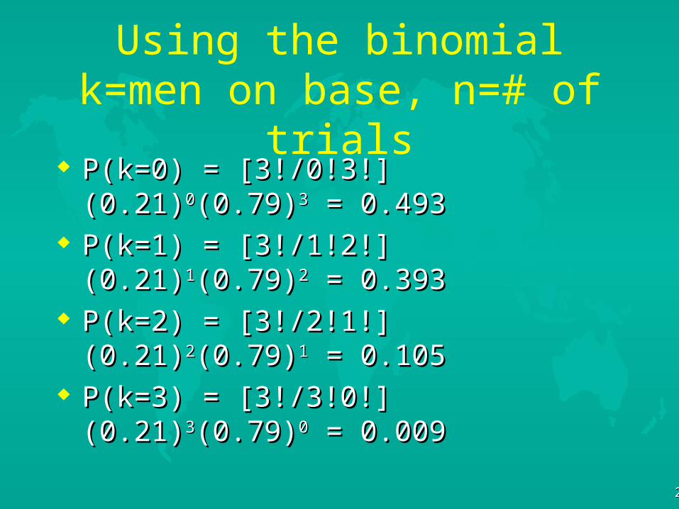
Using the binomialk=men on base, n=# of trials
P(k=0) = [3!/0!3!] (0.21)P(k=0) = [3!/0!3!] (0.21)00(0.79)(0.79)33 = 0.493 = 0.493 P(k=1) = [3!/1!2!] (0.21)P(k=1) = [3!/1!2!] (0.21)11(0.79)(0.79)22 = 0.393 = 0.393 P(k=2) = [3!/2!1!] (0.21)P(k=2) = [3!/2!1!] (0.21)22(0.79)(0.79)11 = 0.105 = 0.105 P(k=3) = [3!/3!0!] (0.21)P(k=3) = [3!/3!0!] (0.21)33(0.79)(0.79)00 = 0.009 = 0.009
2929
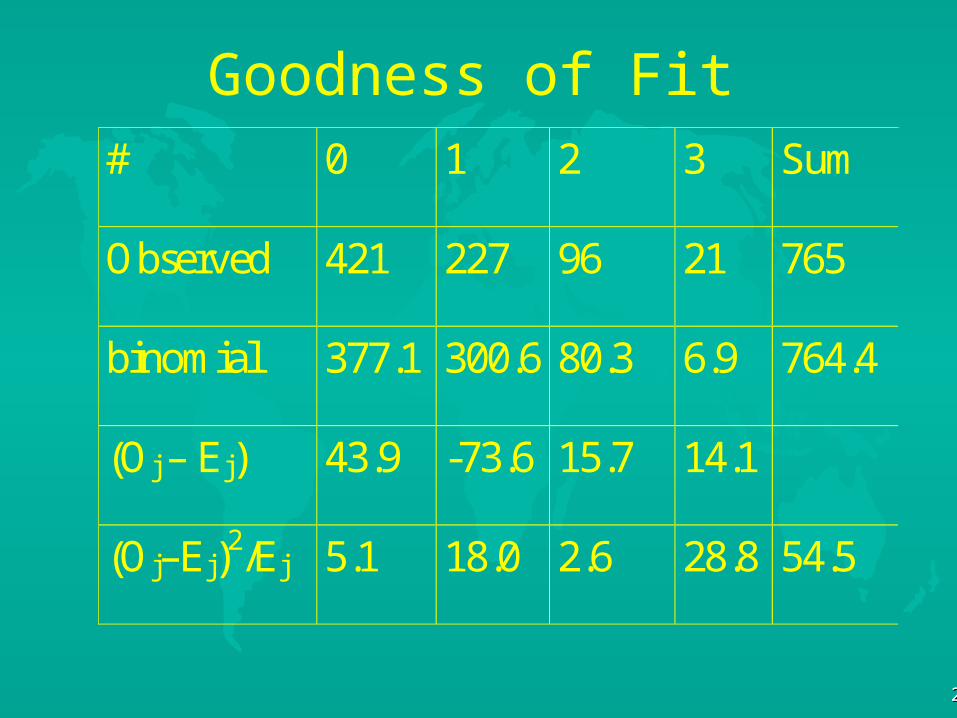
Goodness of Fit# 0 1 2 3 Sum
Observed 421 227 96 21 765
binomial 377.1 300.6 80.3 6.9 764.4
(Oj – Ej) 43.9 -73.6 15.7 14.1
(Oj–Ej)2/Ej 5.1 18.0 2.6 28.8 54.5
0.00
0.05
0.10
0.15
0.20
0.25
0 5 10 15 20
CHI
DE
NS
ITY
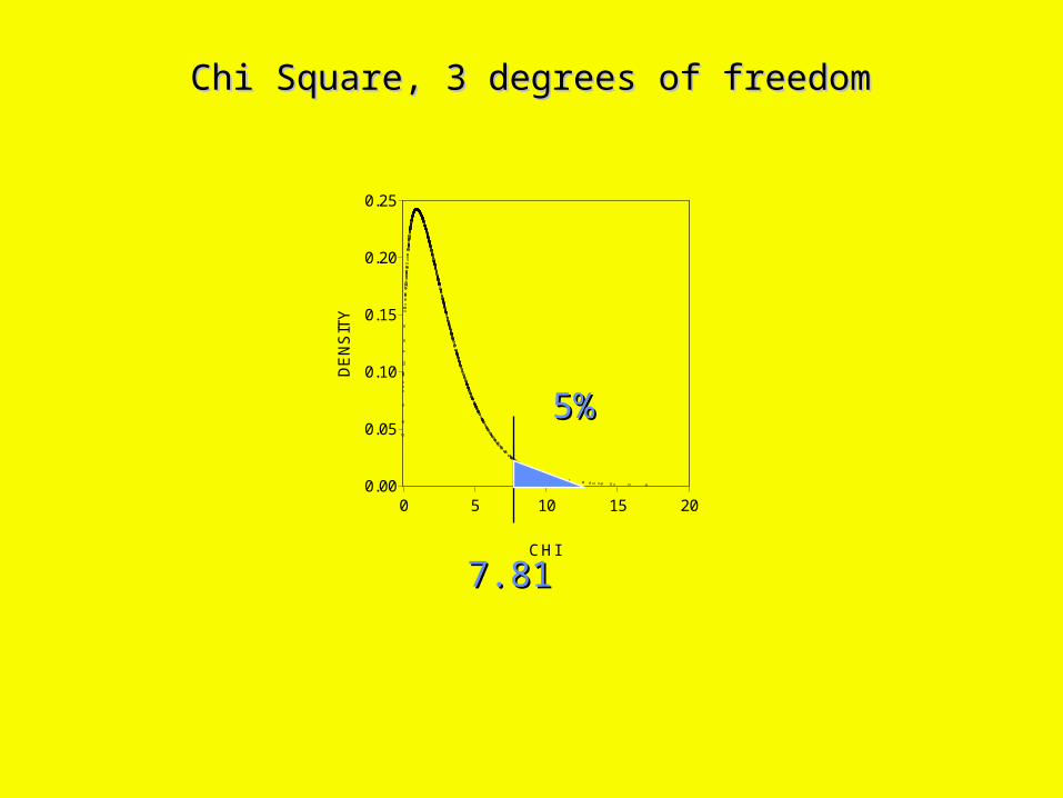
Chi Square, 3 degrees of freedomChi Square, 3 degrees of freedom
5%5%
7.817.81
3131
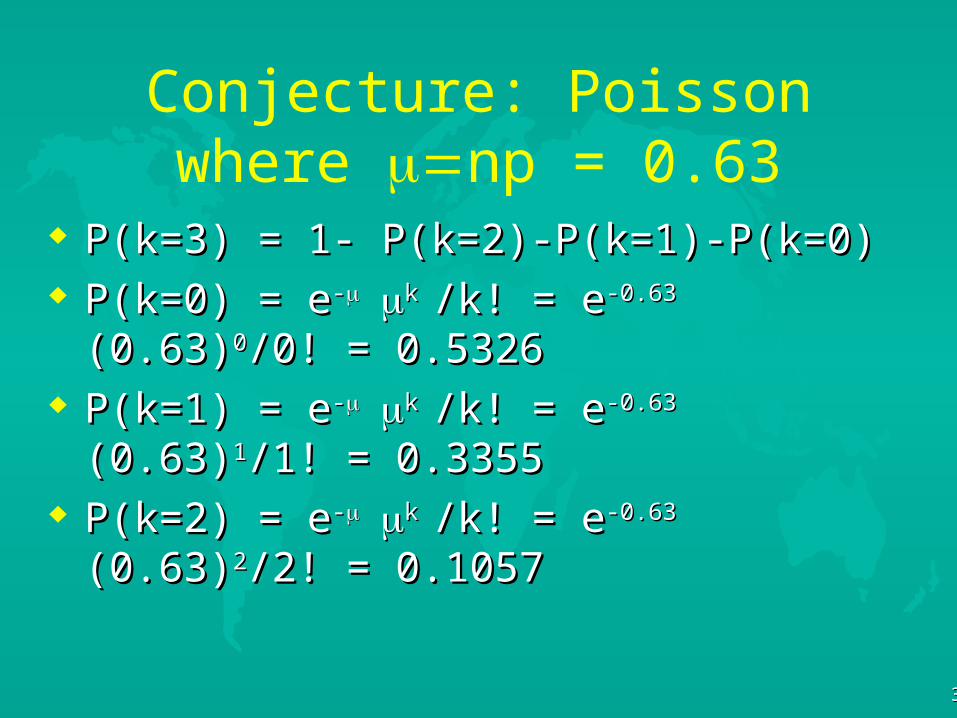
Conjecture: Poisson where np = 0.63
P(k=3) = 1- P(k=2)-P(k=1)-P(k=0)P(k=3) = 1- P(k=2)-P(k=1)-P(k=0) P(k=0) = eP(k=0) = e--k k /k! = e/k! = e-0.63 -0.63 (0.63)(0.63)00/0! = 0.5326/0! = 0.5326 P(k=1) = eP(k=1) = e--k k /k! = e/k! = e-0.63 -0.63 (0.63)(0.63)11/1! = 0.3355/1! = 0.3355 P(k=2) = eP(k=2) = e--k k /k! = e/k! = e-0.63 -0.63 (0.63)(0.63)22/2! = 0.1057/2! = 0.1057
3232
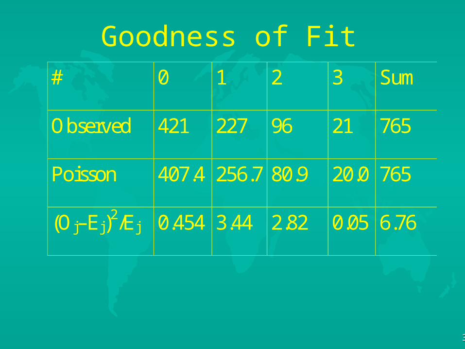
Goodness of Fit# 0 1 2 3 Sum
Observed 421 227 96 21 765
Poisson 407.4 256.7 80.9 20.0 765
(Oj–Ej)2/Ej 0.454 3.44 2.82 0.05 6.76