Poverty, Undernutrition and Intra-household Allocationpeople.ds.cam.ac.uk/ka323/teaching/devt2010/mp-Slides-Lec7.pdf · Prologue Burgess & Zhuang (2002) Nutrition Subramanian & Deaton

Prologue Burgess & Zhuang (2002) Nutrition Subramanian & Deaton

Poverty, Undernutrition and Intra-household

Allocation

EC307 ECONOMIC DEVELOPMENT

Dr. Kumar AniketUniversity of Cambridge & LSE Summer School

Lecture 7created on July 12, 2009

c!Kumar Aniket


READINGS

Tables and figures in this lecture are taken from:

Chapter 8 of Ray (1998)

Chapter 4 of Deaton (1997)

Burgess, R. and Zhuang, J. (2002), Modernisation and SonPreference. mimeo, LSE.

! Class based on Subramanian, S. and Deaton, A. (1996): TheDemand for Food and Calories. Journal of Political Economy, 104(1).

c!Kumar Aniket


INTRODUCTION

So far: Question of the welfare of nations and households

Need to tackle the issue of intra-household allocation, i.e., areresources within household fungible?

– If yes, what the welfare implications of that.

Empirical question:

– Are there biases in the intra-household allocation of resources?

– If there are biases (i.e., imperfect fungibility) – standard householdwelfare measures (e.g., per capita expenditure or income) may notreflect the welfare of household members.

Fungible: mutually interchangeable

c!Kumar Aniket


HOUSEHOLD AND INDIVIDUAL LEVEL DATA

Welfare, Living Standards, Poverty:

– fundamentally characteristics of individuals not households

– expression at household level is just reflects data limitations.

If all household members not treated equally,

e.g., women get less than men, girls less than boys or if children and the elderly

systematically worse off than other household members,

then

social welfare is overstated and

inequality is understated.

c!Kumar Aniket


SOURCE OF BIAS

Where does evidence of biases in intra-household allocation comefrom? e.g., demography/census data.

! We find significantly more men than women (relative to what we would

expect on biological grounds) in certain parts of the world. E.g. SouthAsia, East Asia

! The missing women (Sen etc.) taken as evidence of genderdiscrimination.

Demographic data: skewed sex ratios may be explained by

– big differences between male & female mortality rates in early life

– lower female life expectancy

c!Kumar Aniket

Emily Oster and the Hepatitis B explantion for the missing women


BENCHMARK

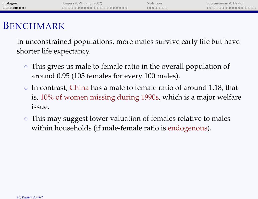
In unconstrained populations, more males survive early life but haveshorter life expectancy.

! This gives us male to female ratio in the overall population ofaround 0.95 (105 females for every 100 males).

! In contrast, China has a male to female ratio of around 1.18, thatis, 10% of women missing during 1990s, which is a major welfareissue.

! This may suggest lower valuation of females relative to maleswithin households (if male-female ratio is endogenous).

c!Kumar Aniket


SON PREFERENCE

Education data: literacy and enrolment rates for females muchlower than those for males.

Can son preference be viewed as structural feature of developingcountries?

Problem: Mechanisms underlying these differences are not fullyunderstood.

c!Kumar Aniket


ONE PARTICULAR VIEW

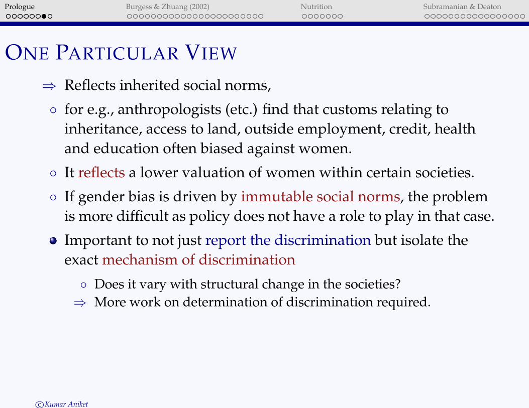
" Reflects inherited social norms,

! for e.g., anthropologists (etc.) find that customs relating toinheritance, access to land, outside employment, credit, healthand education often biased against women.

! It reflects a lower valuation of women within certain societies.

! If gender bias is driven by immutable social norms, the problemis more difficult as policy does not have a role to play in that case.

Important to not just report the discrimination but isolate theexact mechanism of discrimination

! Does it vary with structural change in the societies?" More work on determination of discrimination required.

c!Kumar Aniket


DETECTING GENDER BIASES

Problem with the literature:

Descriptive, quantitative analysis to date has been largelyconfined to census data on mortality and enrolment ratesdifferenced by sex

Doesn’t allow us to examine driving factors behind genderbiases.

The behavioural mechanisms that underlie differential outcomesbetween the sexes remain not clearly understood.

c!Kumar Aniket


Modernisation and Son Preference

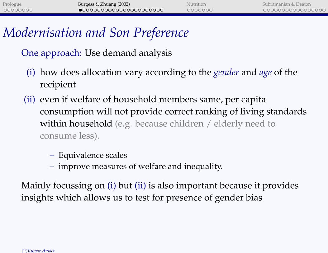
One approach: Use demand analysis

(i) how does allocation vary according to the gender and age of therecipient

(ii) even if welfare of household members same, per capitaconsumption will not provide correct ranking of living standardswithin household (e.g. because children / elderly need toconsume less).

– Equivalence scales– improve measures of welfare and inequality.

Mainly focussing on (i) but (ii) is also important because it providesinsights which allows us to test for presence of gender bias

c!Kumar Aniket


UNPACKING THE DEMAND EQUATIONS

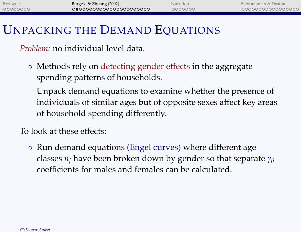
Problem: no individual level data.

! Methods rely on detecting gender effects in the aggregatespending patterns of households.

Unpack demand equations to examine whether the presence ofindividuals of similar ages but of opposite sexes affect key areasof household spending differently.

To look at these effects:

! Run demand equations (Engel curves) where different ageclasses nj have been broken down by gender so that separate !ij

coefficients for males and females can be calculated.

c!Kumar Aniket


ENGLE CURVES

wi = "i +#i lnx+$i lnn+J#1

%j=1

!ij

!

nj

n

"

+&iz+ui

where

wi is the budget share of the ith commodity,

x the total household expenditure,

n the household size,

nj is number of household members in sex-ageclass j.

z vector of variables which control for locationand relevant socio-economic characteristics ofthe household.

Test of gender bias:

!ij = !ik,

where j and k reflect boys and girlsin the same age group.

The hypothesis of equal treatment

can be tested in a straightforward

manner using an F test.

c!Kumar Aniket


ENGLE CURVES

Run two types of variables on left hand side:

(i) Goods that are considered to be integral to welfare of children(i.e., food, health, education).

$ Differential treatment in these areas may have permanent andirreversible welfare effects.

The question is does adding a boy relative to a girl lead to lower/ higher expenditures on these goods assuming that

! children are exogenousnot contributing resources to household andnot involved in food, health, education allocation decisions.

c!Kumar Aniket


ENGLE CURVES

Run two types of variables on left hand side:

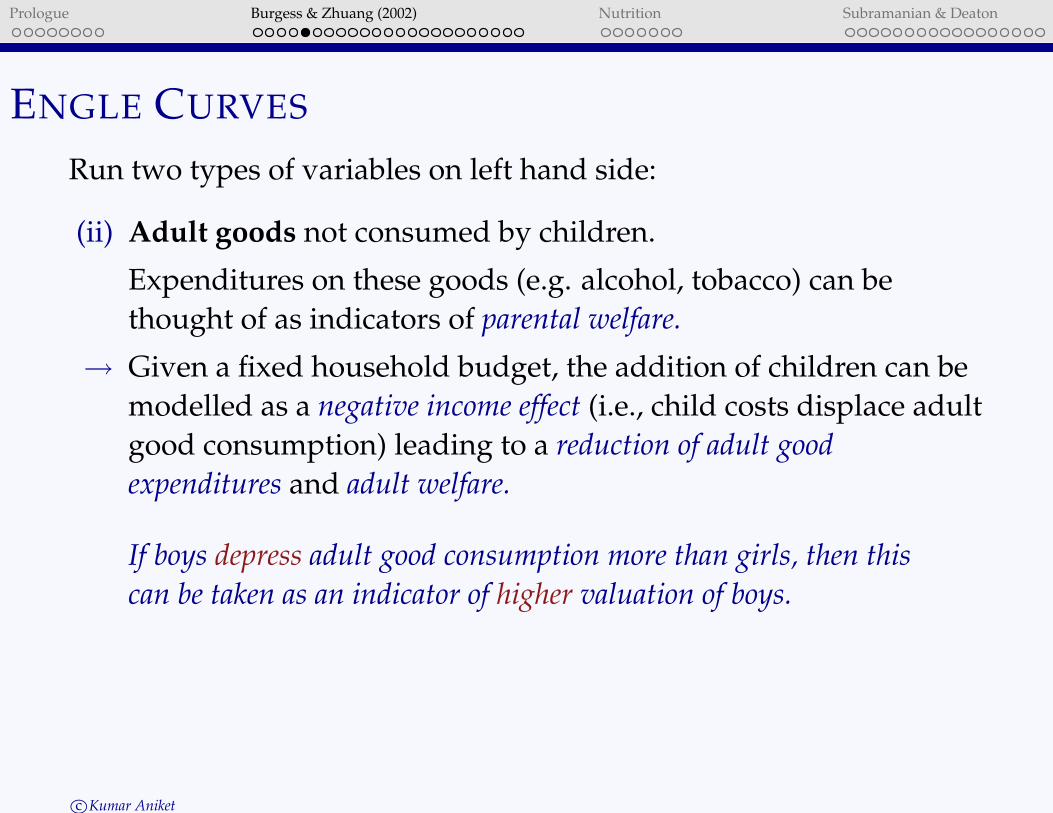
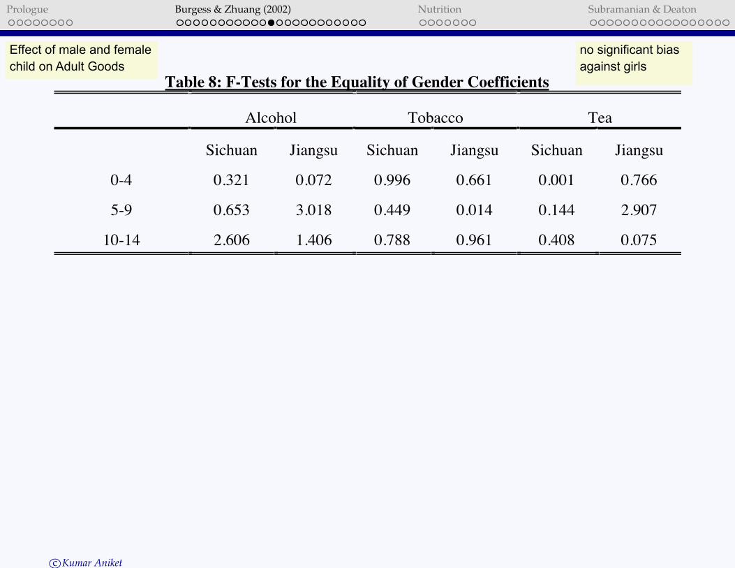
(ii) Adult goods not consumed by children.

Expenditures on these goods (e.g. alcohol, tobacco) can bethought of as indicators of parental welfare.

$ Given a fixed household budget, the addition of children can bemodelled as a negative income effect (i.e., child costs displace adultgood consumption) leading to a reduction of adult goodexpenditures and adult welfare.

If boys depress adult good consumption more than girls, then thiscan be taken as an indicator of higher valuation of boys.

c!Kumar Aniket


ADULT EQUIVALENT RATIO

For adult goods, from equation above, we can calculate “adultequivalent ratio,”

i.e., how much would total expenditure have to be reduced to result in areduction in expenditure on goods i equal to that observed by theaddition of a child of type j to the household.

'ij =

#

(piqi

(nj

$

#

(piqi

(x

$ ·n

x=

%

$i + !ij&

#%j=1J#1 !ij

'

nj

n

(

#i +wi

c!Kumar Aniket


ADULT EQUIVALENT RATIO

Then can look at three things

(i) whether 'ij < 0.

(ii) test of whether 'ij = 'hj,

where i and h are different potential adult goods, that is, test of whether

they are valid adult goods

(iii) test whether 'ib = 'ig

where b and g denote boy and girl. Test of gender bias.

Equivalent to doing an F test on whether !ij = !ik,

where j and k reflect boys and girls in the same age group in regression

where adult good share wi is the left hand side variable.

c!Kumar Aniket


EMPIRICAL EVIDENCE

Deaton (1997): direct comparison by gender of nutrition, health andeducation reveals gender biases.

For example, excess female mortality amongst girls in China,Bangladesh and India.

Further, enrolment and literacy tend to be higher for boys rather thangirls (in cohorts of the same age) in many parts of the developingword.

c!Kumar Aniket


EMPIRICAL EVIDENCE

Mechanisms that underlie these differences are not fully understood.

One suggestion, for example, is that excess female mortality is due tofemale children receiving less medical attention when they are sick.

Burgess and Zhuang (2001) use household expenditure to try and pryopen this black box for China.

c!Kumar Aniket


Table 3: Health Engel Curves, 1990

Health goods Health services

Sichuan Jiangsu Sichuan Jiangsu

Constant -1.108 (1.025) 0.409 (0.339) -1.885 (-4.691) -2.072 (-1.959)

ln(x) 0.483 (3.774) 0.300 (2.211) 0.323 (6.434) 0.306 (2.570)

ln(n) -0.481 (-2.865) -0.421 (1.884) -0.181(-2.752) 0.174 (0.888)

M0-4p 2.002 (2.989) 2.710 (3.059) 0.552 (2.104) 2.120 (2.730)

F0-4p 0.419 (0.621) 3.730 (4.172) 0.559 (2.111) 1.646 (2.100)

M5-9p 0.709 (1.049) 1.702 (1.901) 0.287 (1.083) 0.239 (0.304)

F5-9p 0.325 (0.477) -1.125 (1.198) -0.240 (-0.902) 1.433 (1.741)

M10-14p -0.729 (-1.123) 0.558 (0.621) -0.020 (-0.079) 1.774 (2.254)

F10-14p -0.959 (-1.481) 0.863 (0.971) -0.240 (-0.944) 0.816 (1.048)

M15-19p -1.077 (-1.827) -0.096 (-0.118) -0.062 (-0.267) 0.383 (0.532)

F15-19p -0.413 (-0.697) 0.761 (0.900) 0.029 (0.232) 0.253 (0.341)

M20-29p -1.282 (-2.363) -0.379 (-0.519) -0.022(-0.102) 0.147 (0.230)

F20-29p 0.363 (0.635) 1.045 (1.551) 0.369 (1.953) 0.216 (0.365)

M30-54p -0.006 (-0.010) 0.391 (0.481) 0.412 (1.810) 0.298 (0.418)

M55+p 0.740 (1.302) -0.390 (0.514) 0.496 (2.228) 0.567 (0.852)

F55+p 1.233 (2.506) 0.499 (0.793) 0.345 (1.787) 0.529 (0.959)

EDU 0.056 (1.030) -0.145 (-2.213) -0.021(-0.986) -0.089 (-1.553)

OFF 0.223 (1.094) -0.170 (-0.649) -0.053(-0.663) 0.117 (0.506)

MIN -1.252 (-3.686) -1.347 (-1.660) -0.342(-2.566) -1.089 (-1.531)

Adj R2

0.058 0.026 0.026 0.045

Mean wi 2.089 1.609 0.424 0.793

F tests:

0-4 6.07 1.00 0.00 0.33

5-9 0.41 0.43 0.04 2.48

10-14 0.19 0.17 1.10 1.78

Note: t-statistics in parentheses.c!Kumar Aniket

erosion of gender

biases through

modernisation

health services

subsidisedF tests: Testing the null hypothesis that coefficients for a male and girl child of a particular age group are equal.

A sufficiently high F value indicates that they are not.


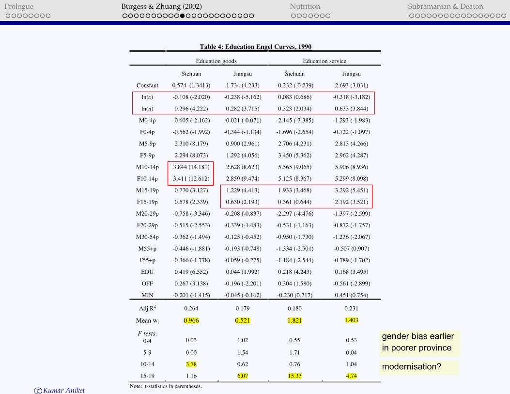
Table 4: Education Engel Curves, 1990

Education goods Education service

Sichuan Jiangsu Sichuan Jiangsu

Constant 0.574 (1.3413) 1.734 (4.233) -0.232 (-0.239) 2.693 (3.031)

ln(x) -0.108 (-2.020) -0.238 (-5.162) 0,083 (0.686) -0.318 (-3.182)

ln(n) 0.296 (4.222) 0.282 (3.715) 0.323 (2.034) 0.633 (3.844)

M0-4p -0.605 (-2.162) -0.021 (-0.071) -2.145 (-3.385) -1.293 (-1.983)

F0-4p -0.562 (-1.992) -0.344 (-1.134) -1.696 (-2.654) -0.722 (-1.097)

M5-9p 2.310 (8.179) 0.900 (2.961) 2.706 (4.231) 2.813 (4.266)

F5-9p 2.294 (8.073) 1.292 (4.056) 3.450 (5.362) 2.962 (4.287)

M10-14p 3.844 (14.181) 2.628 (8.623) 5.565 (9.065) 5.906 (8.936)

F10-14p 3.411 (12.612) 2.859 (9.474) 5.125 (8.367) 5.299 (8.098)

M15-19p 0.770 (3.127) 1.229 (4.413) 1.933 (3.468) 3.292 (5.451)

F15-19p 0.578 (2.339) 0.630 (2.193) 0.361 (0.644) 2.192 (3.521)

M20-29p -0.758 (-3.346) -0.208 (-0.837) -2.297 (-4.476) -1.397 (-2.599)

F20-29p -0.515 (-2.553) -0.339 (-1.483) -0.531 (-1.163) -0.872 (-1.757)

M30-54p -0.362 (-1.494) -0.125 (-0.452) -0.950 (-1.730) -1.236 (-2.067)

M55+p -0.446 (-1.881) -0.193 (-0.748) -1.334 (-2.501) -0.507 (0.907)

F55+p -0.366 (-1.778) -0.059 (-0.275) -1.184 (-2.544) -0.789 (-1.702)

EDU 0.419 (6.552) 0.044 (1.992) 0.218 (4.243) 0.168 (3.495)

OFF 0.267 (3.138) -0.196 (-2.201) 0.304 (1.580) -0.561 (-2.899)

MIN -0.201 (-1.415) -0.045 (-0.162) -0.230 (0.717) 0.451 (0.754)

Adj R2

0.264 0.179 0.180 0.231

Mean wi 0.966 0.521 1.821 1.403

F tests:

0-4 0.03 1.02 0.55 0.53

5-9 0.00 1.54 1.71 0.04

10-14 3.78 0.62 0.76 1.04

15-19 1.16 6.07 15.33 4.74

Note: t-statistics in parentheses.c!Kumar Aniket

gender bias earlier

in poorer province

modernisation?


Table 8: F-Tests for the Equality of Gender Coefficients

Alcohol Tobacco Tea

Sichuan Jiangsu Sichuan Jiangsu Sichuan Jiangsu

0-4 0.321 0.072 0.996 0.661 0.001 0.766

5-9 0.653 3.018 0.449 0.014 0.144 2.907

10-14 2.606 1.406 0.788 0.961 0.408 0.075

c!Kumar Aniket

no significant bias

against girls

Effect of male and female

child on Adult Goods


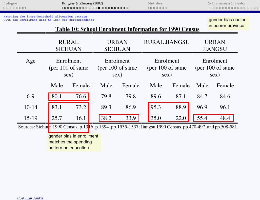
Table 10: School Enrolment Information for 1990 Census

RURAL

SICHUAN

URBAN

SICHUAN

RURAL JIANGSU URBAN

JIANGSU

Enrolment

(per 100 of same

sex)

Enrolment

(per 100 of same

sex)

Enrolment

(per 100 of same

sex)

Enrolment

(per 100 of same

sex)

Age

Male Female Male Female Male Female Male Female

6-9 80.1 76.6 79.8 79.8 89.6 87.1 84.7 84.6

10-14 83.1 73.2 89.3 86.9 95.3 88.9 96.9 96.1

15-19 25.7 16.1 38.2 33.9 35.0 22.0 55.4 48.4

Sources: Sichuan 1990 Census, p.1316, p.1394, pp.1535-1537; Jiangsu 1990 Census, pp.470-497, and pp.508-581.

c!Kumar Aniket

gender bias earlier

in poorer province

gender bias in enrollment

matches the spending

pattern on education

Matching the intra-household allocation pattern with the Enrollment data to look for correspondence


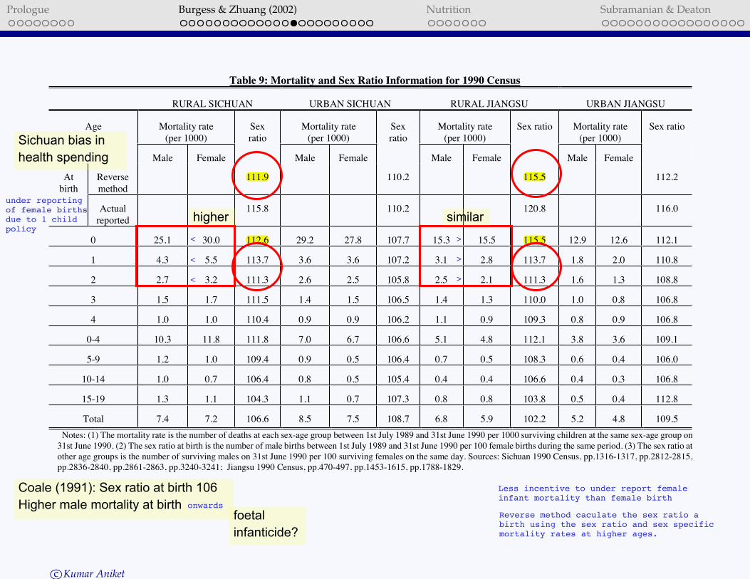
Table 9: Mortality and Sex Ratio Information for 1990 Census

RURAL SICHUAN URBAN SICHUAN RURAL JIANGSU URBAN JIANGSU

Mortality rate

(per 1000)

Mortality rate

(per 1000)

Mortality rate

(per 1000)

Mortality rate

(per 1000)

Age

Male Female

Sex

ratio

Male Female

Sex

ratio

Male Female

Sex ratio

Male Female

Sex ratio

Reverse

method

111.9 110.2 115.5 112.2At

birth

Actual

reported

115.8 110.2 120.8 116.0

0 25.1 30.0 112.6 29.2 27.8 107.7 15.3 15.5 115.5 12.9 12.6 112.1

1 4.3 5.5 113.7 3.6 3.6 107.2 3.1 2.8 113.7 1.8 2.0 110.8

2 2.7 3.2 111.3 2.6 2.5 105.8 2.5 2.1 111.3 1.6 1.3 108.8

3 1.5 1.7 111.5 1.4 1.5 106.5 1.4 1.3 110.0 1.0 0.8 106.8

4 1.0 1.0 110.4 0.9 0.9 106.2 1.1 0.9 109.3 0.8 0.9 106.8

0-4 10.3 11.8 111.8 7.0 6.7 106.6 5.1 4.8 112.1 3.8 3.6 109.1

5-9 1.2 1.0 109.4 0.9 0.5 106.4 0.7 0.5 108.3 0.6 0.4 106.0

10-14 1.0 0.7 106.4 0.8 0.5 105.4 0.4 0.4 106.6 0.4 0.3 106.8

15-19 1.3 1.1 104.3 1.1 0.7 107.3 0.8 0.8 103.8 0.5 0.4 112.8

Total 7.4 7.2 106.6 8.5 7.5 108.7 6.8 5.9 102.2 5.2 4.8 109.5

Notes: (1) The mortality rate is the number of deaths at each sex-age group between 1st July 1989 and 31st June 1990 per 1000 surviving children at the same sex-age group on

31st June 1990. (2) The sex ratio at birth is the number of male births between 1st July 1989 and 31st June 1990 per 100 female births during the same period. (3) The sex ratio at

other age groups is the number of surviving males on 31st June 1990 per 100 surviving females on the same day. Sources: Sichuan 1990 Census, pp.1316-1317, pp.2812-2815,

pp.2836-2840, pp.2861-2863, pp.3240-3241; Jiangsu 1990 Census, pp.470-497, pp.1453-1615, pp.1788-1829.

c!Kumar Aniket

foetal

infanticide?

Sichuan bias in

health spending

Coale (1991): Sex ratio at birth 106

Higher male mortality at birth

similarhigher

onwards

>

>

>

<

<

<

under reporting of female births due to 1 child policy

Less incentive to under report female infant mortality than female birth

Reverse method caculate the sex ratio a birth using the sex ratio and sex specific mortality rates at higher ages.


Table 12: F-tests for the Equality of Gender Coefficients: Degree of Diversification Breakdown

Health Goods Health Services Educational Goods Educational Services

Rural

Sichuan

Rural

Jiangsu

Rural

Sichuan

Rural

Jiangsu

Rural

Sichuan

Rural

Jiangsu

Rural

Sichuan

Rural

Jiangsu

Overall sample

0-4 6.07 1.00 0.00 0.33 0.03 1.02 0.55 0.53

5-9 0.41 0.43 0.04 2.48 0.00 1.54 1.71 0.04

10-14 0.19 0.17 1.10 1.78 3.78 0.62 0.76 1.04

15-19 - - - - 1.16 6.07 15.33 4.74

Bottom ! sample

0-4 6.57 1.54 1.05 0.60 0.16 0.55 0.07 0.90

5-9 0.62 0.12 0.04 1.75 0.00 0.58 0.76 0.00

10-14 0.32 0.83 1.99 3.76 10.81 0.21 6.34 0.08

15-19 - - - - 0.99 3.53 1.73 1.91

Top ! sample

0-4 0.76 0.03 0.99 1.72 0.11 0.64 0.40 0.06

5-9 0.21 0.40 0.28 0.72 0.00 0.71 1.16 0.08

10-14 0.02 2.83 0.01 0.00 0.22 0.64 0.97 1.09

15-19 - - - - 0.15 1.46 13.02 1.62

c!Kumar Aniket

lower the level of diversification, the

higher the level of gender bias


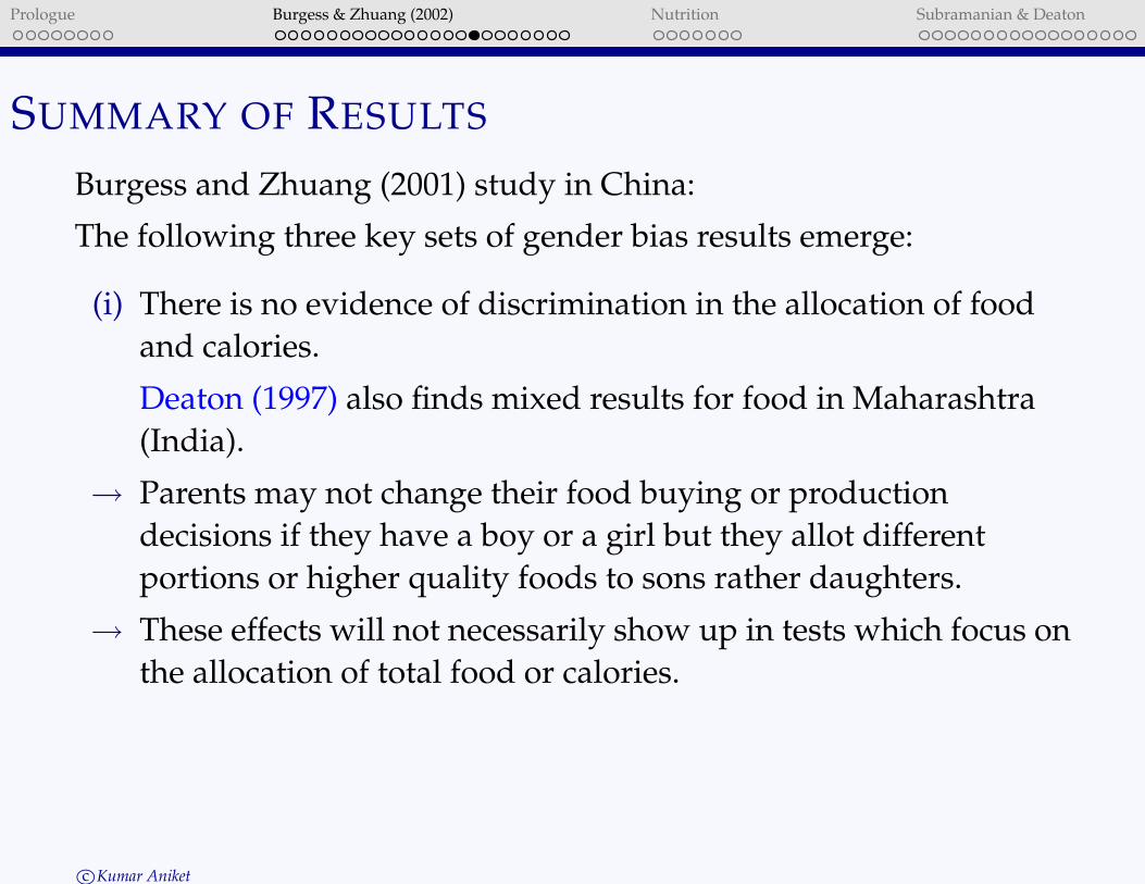
SUMMARY OF RESULTS

Burgess and Zhuang (2001) study in China:

The following three key sets of gender bias results emerge:

(i) There is no evidence of discrimination in the allocation of foodand calories.

Deaton (1997) also finds mixed results for food in Maharashtra(India).

$ Parents may not change their food buying or productiondecisions if they have a boy or a girl but they allot differentportions or higher quality foods to sons rather daughters.

$ These effects will not necessarily show up in tests which focus onthe allocation of total food or calories.

c!Kumar Aniket


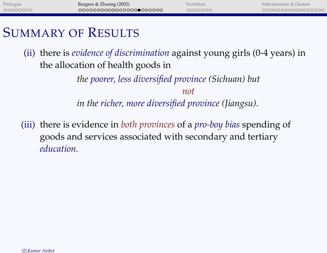
SUMMARY OF RESULTS

(ii) there is evidence of discrimination against young girls (0-4 years) inthe allocation of health goods in

the poorer, less diversified province (Sichuan) butnot

in the richer, more diversified province (Jiangsu).

(iii) there is evidence in both provinces of a pro-boy bias spending ofgoods and services associated with secondary and tertiaryeducation.

c!Kumar Aniket


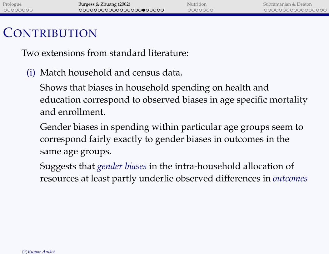
CONTRIBUTION

Two extensions from standard literature:

(i) Match household and census data.

Shows that biases in household spending on health andeducation correspond to observed biases in age specific mortalityand enrollment.

Gender biases in spending within particular age groups seem tocorrespond fairly exactly to gender biases in outcomes in thesame age groups.

Suggests that gender biases in the intra-household allocation ofresources at least partly underlie observed differences in outcomes

c!Kumar Aniket


CONTRIBUTION

Two extensions from standard literature:

(ii) Comparisons across and within (rural and urban) samplesconfirm that discrimination in health good spending against girls0-4 years of age, associated with poorer, less diversifiedhouseholds.

$ Same pattern of results is also found for spending on educationgoods.

Results suggest that income and the composition of income enterinto the parental decision rule.

$ Discrimination is not driven entirely by cultural factors.

c!Kumar Aniket


CONTRIBUTION

This points to a potential serole for public policy in counteractinggender discrimination.

As regards excess female mortality in the 0-5 age group, it wouldappear that policies which promote growth and diversification willreduce this form of gender discrimination.

Households in rural Jiangsu, which do not show evidence of excessfemale mortality in the 0-5 age range, however, appear to adjust sexcomposition prior to birth, most probably through screening andselective abortion.

c!Kumar Aniket


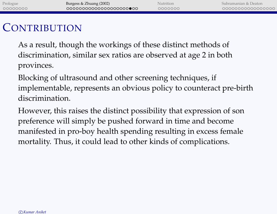
CONTRIBUTION

As a result, though the workings of these distinct methods ofdiscrimination, similar sex ratios are observed at age 2 in bothprovinces.

Blocking of ultrasound and other screening techniques, ifimplementable, represents an obvious policy to counteract pre-birthdiscrimination.

However, this raises the distinct possibility that expression of sonpreference will simply be pushed forward in time and becomemanifested in pro-boy health spending resulting in excess femalemortality. Thus, it could lead to other kinds of complications.

c!Kumar Aniket


CONTRIBUTION

Education: broad suggestion that growth and diversification helpserode these forms of discrimination.

It may reflect both the roles these processes have to play in equalisingreturns to males and females (e.g., in off-farm employment) and ineroding cultural beliefs, which favour focussing secondary and tertiaryeducation on males.

This paper cannot discriminate between these two effects - both arelikely to be going on.

c!Kumar Aniket


PROBLEMS

Adult goods: It is difficult to find any results even when censusindicates presence of discrimination. See Deaton (1997) for a review.

Problems:

(i) difficult to identify adults goods

(ii) they constitute small part of total expenditure

(iii) children may actually contribute resources to household

(iv) children may change tastes of adults

c!Kumar Aniket


INTRODUCTION TO NUTRITION

! Development economics’ objective: Improve human welfare.

However, welfare is multidimensional,

– e.g., income and nutrition have many dimensions

– being poor and being undernourished are not the same thing.

Big question: Will rising economic welfare (associated, for example,with economic diversification and the green revolution) lead toreductions in calorific undernutrition?

Until recently, it was widely accepted in international policycircles that income growth has an important role to play inimproving the nutrition of the poor.

c!Kumar Aniket


INCOME NUTRITION LINK

! Recent studies like Behrman and Deolalikar has questioned thestrength of the association between income and nutrition.

Changes in income $ small impact on nutrient intake

! Policy implication: Income mediated policies will have limited impacton nutritional goals.

! Governments will have to supplement income generationprogrammes with alternative strategies

– i.e., price subsidies, rationing, feeding programmes, nutritionand education to limit hunger and malnutrition.

c!Kumar Aniket


TWO VIEWS

There is also common ground between two distinct views

One View

Treats household welfare(including nutrition) assynonymous with householdincome

Other View

Views household welfare interms the capability to avoidbasic deprivations, includingundernutrition, which is

View eroded if income growth isnot associated withimprovements in nutrition.

Shrinking ground makes it difficult to think of household income as aconvenient shorthand for household welfare.

c!Kumar Aniket


For public policy, nutritional welfare and economic welfare wouldhave to be considered separately.

Two versions of “revisionist” positions:

i. Strong version: No association between income growth andimprovements in nutrition, or at least none that is statisticallydiscernible (Behrman and Deolalikar, 1987).

ii. Weak version: Response of nutrition to income among the poor isstatistically significant but small. The hypothesis does not deny therole of income growth in improving nutrition, it emphasizes itsweakness.

c!Kumar Aniket


LINKING INCOME TO NUTRITION

Size of the calorie response is an an empirical question, which can, inprinciple, be determined with reference to relevant data.

Households in developing countries typically spend a largeproportion of their income on food

e.g., 50%-70%

Elasticity of demand for food with respect to income (ratherexpenditure) is therefore quite high for a substantial proportion ofthe population and may even be close to one for the pooresthouseholds.

c!Kumar Aniket


LINKING INCOME TO NUTRITION

This does not necessarily imply an equally high elasticity of demandfor calories.

As expenditure rises, households switch towards more expensivefoods, which involves both:

i. substitution within broad food groups towards higher qualityfoods (“superior” cereals like rice in place of ‘coarse’ cereals likesorghum or maize), and

ii. substitution between food groups (meat, dairy products or fats inplace of cereals).

Price per unit calorie is thus an increasing function of income.

Elasticity of calories therefore lies below the elasticity of food.

c!Kumar Aniket


c!Kumar Aniket

Adjusted for meal given/receivedExpenditure 115 28248

As income increases, food patterns change with price per calorie of food items increasing

SorghumMillet


FOOD AND CALORIE ELASTICITY

Substitution towards higher priced calories drives a wedge betweenfood elasticity and calorie elasticity.

The size of this wedge depends on household preferences forquality and variety at the margin.

Expect the switch to expensive foods to be more pronounced athigh levels of per-capita expenditure.

Calorie-expenditure elasticity will therefore tend to decline towardszero as expenditure rises.

Whether the elasticity is as low as 0.10 (or even 0.0) at low intakesis what is in dispute.

– Estimates range from around 0.5 on the one hand to near zeroon the other.

c!Kumar Aniket


CALORIE RESPONSE

Problem: Elasticity evaluated at mean as opposed to in the lowerend of distribution. However, controversy is over the size of thecalorie response in poor households.

Benchmark: Reutlinger and Selowsky (1976): calorie elasticities ofaround 0.3 – 0.4 in the poorest households, which falls as calorieavailability increases.

– High estimates reported in the literature broadly reinforce thebenchmark values.

Revisionist: Calorie response is considerably smaller, even in poorhouseholds – closer to a third or a quarter of what was previouslyassumed.

Extreme view: Calorie–expenditure curve is essentially flat over thewhole range of per-capita expenditure.

c!Kumar Aniket


BIASED CALORIE ELASTICITIES: MEASUREMENT

ERROR

Variation in size of calorie elasticities is in part due to differences inthe method of data collection.

Estimates obtained from nutritional surveys based on 24-hourobservation or recall of food consumption tend to be lower than thosebased on household expenditure surveys. Why?

i. Measurement error in expenditure surveys: Food quantities typicallyfigure in the construction of both calories and householdexpenditure.

Any error in the measurement of food is transmitted by construction toboth variables (e.g., in imputation of home produced consumption).

c!Kumar Aniket


BIASED CALORIE ELASTICITIES: MEASUREMENT

ERROR

Spurious positive correlation between calorie availability andhousehold expenditure, which would tend to bias the estimatedelasticity upwards.

Solution: Instrumental Variables – Variables used as instrumentsmust be correlated with household expenditure and arguablyuncorrelated with its measurement error.E.g., income if independently measured, proxies of long-termincome or wealth are other candidates.

Use of instrumental variables leads to a small fall in the estimatedelasticity. Fall is not sufficient to place the estimated elasticity inthe ‘revisionist’ camp (e.g. Subramanian and Deaton, 1998).

Difference between estimates cannot be ascribed tomethodological differences alone.

c!Kumar Aniket


BIASED CALORIE ELASTICITIES: MISREPORTING

ii. Misreporting of food consumption: May be more pronounced in thecase of expenditure surveys as opposed to 24-hour nutritionsurveys.

Food intakes are not directly measured in expenditure surveys,

Food may be given to guests, agricultural labourers, servants or even animals but

nonetheless recorded as household consumption.

Food consumption by non-members is systematically related tohousehold expenditure (richer households have more servants, hiremore labour, feed more guests and own more livestock).

This will lead to an overstatement (understatement) of calorieavailability in richer (poorer) households. Impart an upward biasto calorie elasticities.

c!Kumar Aniket


BIASED CALORIE ELASTICITIES

Solution: Don’t look at mean elasticity but rather at specific parts ofthe distribution.

Non-parametric regression within narrow income band (e.g.,bottom quintile). Scope for this being a problem limited within anarrow income band.

Deaton (1997): Warns against presuming that nutrition surveysprovide superior data. Increased accuracy from observation could beoffset by the artificial and intrusive nature of the survey.

To avoid embarrassment, poor households may consume more onthe day of observation than is average. Similarly, people mayreport better diets than actually consumed. These factors wouldcompress the lower extreme and lead to a downward bias in thecalorie elasticity.

c!Kumar Aniket


THE DEMAND FOR FOOD AND CALORIES

Methodology: Three distinct methods to get calorie elasticityestimates

i. Non-parametric regression

ii. Ordinary least squares (OLS) regression

iii. Instrumental variable (IV) regression

c!Kumar Aniket


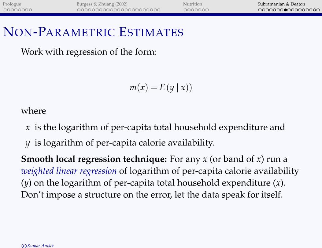
NON-PARAMETRIC ESTIMATES

Work with regression of the form:

m(x) = E(y | x))

where

x is the logarithm of per-capita total household expenditure and

y is logarithm of per-capita calorie availability.

Smooth local regression technique: For any x (or band of x) run aweighted linear regression of logarithm of per-capita calorie availability(y) on the logarithm of per-capita total household expenditure (x).Don’t impose a structure on the error, let the data speak for itself.

c!Kumar Aniket


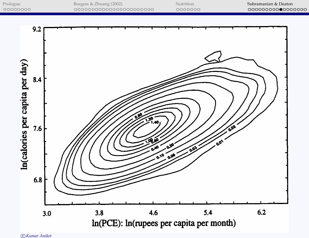
NON-PARAMETRIC REGRESSIONS

Non-parametric regression: Useful for examining bi-variaterelationships, which are potentially non-linear. Look at the shape ofrelationship – is there flattening with increasing income?

$ Use average derivative estimators to calculate the slopes withindifferent bands of x. Allows us to graph out calorie elasticities. Lookfor two things:

i. Is there a decline in elasticity with increasing income.

ii. Are calorie elasticity estimates significantly different from zero, inparticular for the poor. Calculate the confidence intervals to checkthis.

c!Kumar Aniket


c!Kumar Aniket


c!Kumar Aniket


c!Kumar Aniket


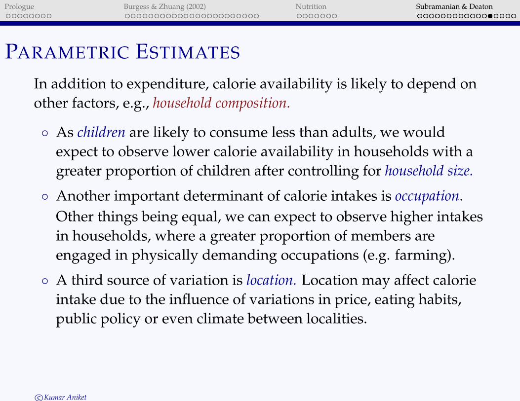
PARAMETRIC ESTIMATES

In addition to expenditure, calorie availability is likely to depend onother factors, e.g., household composition.

! As children are likely to consume less than adults, we wouldexpect to observe lower calorie availability in households with agreater proportion of children after controlling for household size.

! Another important determinant of calorie intakes is occupation.

Other things being equal, we can expect to observe higher intakesin households, where a greater proportion of members areengaged in physically demanding occupations (e.g. farming).

! A third source of variation is location. Location may affect calorieintake due to the influence of variations in price, eating habits,public policy or even climate between localities.

c!Kumar Aniket


ENGLE CURVE

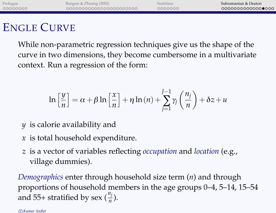
While non-parametric regression techniques give us the shape of thecurve in two dimensions, they become cumbersome in a multivariatecontext. Run a regression of the form:

ln) y

n

*

= "+# ln) x

n

*

+$ ln(n)+J#1

%j=1

!j

!

nj

n

"

+&z+u

y is calorie availability and

x is total household expenditure.

z is a vector of variables reflecting occupation and location (e.g.,village dummies).

Demographics enter through household size term (n) and throughproportions of household members in the age groups 0–4, 5–14, 15–54and 55+ stratified by sex (

nj

n ).

c!Kumar Aniket


OLS ESTIMATE

OLS estimates may be biased as food consumption data may besubject to random error that feeds into the construction of bothhousehold expenditure and calorie availability.

This form of measurement error may be corrected for using incomeas an instrument for expenditure if this is available and collectedindependently of expenditure, for e.g., non-food expenditure.(Deaton, 1997)

c!Kumar Aniket


c!Kumar Aniket


SUMMARY

Calorie availability is strongly associated with household economicwelfare.

! Subramaniam and Deaton (1996) observe high calorie elasticities ofaround 0.55 for the poor in rural Maharashtra which is welloutside the revisionist range.

! Findings clearly refute the extreme view that, “increases inincome . . . will not result in substantial improvements in nutrientintakes?” (Behrman and Deolalikar ,1987, page 505)

• Economic development, as proxied by rising household expenditure,will lead to reductions in calorific undernutrition, which is animportant finding from the perspective of public policy.

c!Kumar Aniket

Documents

Poverty, Undernutrition and Intra-household Allocationpeople.ds.cam.ac.uk/ka323/teaching/devt2010/mp-Slides-Lec7.pdf · Prologue Burgess & Zhuang (2002) Nutrition Subramanian & Deaton