Poverty and Equity:Theory and Estimation

by

Jean-Yves Duclos

Departement d’economique and CREFA,Universite Laval, Canada

Preliminary version

This text is in large part an output of the MIMAP training programme financedby the International Development Research Center of the Government of Canada.The underlying research was also supported by grants from the Social Sciencesand Humanities Research Council of Canada and from the Fonds FCAR of theProvince of Quebec. I am grateful to Abdelkrim Araar and Nicolas Beaulieu fortheir excellent research assistance.

Corresponding address:Jean-Yves Duclos, Departement d’economique, Pavillon de Seve, Universite

Laval, Quebec, Canada, G1K 7P4; Tel.: (418) 656-7096; Fax: (418) 656-7798;Email: jduc@ecn.ulaval.ca

January 2002

Contents

I Introduction 5

1 Well-being and poverty 61.1 The welfarist approach. . . . . . . . . . . . . . . . . . . . . . . 61.2 Non-welfarist approaches. . . . . . . . . . . . . . . . . . . . . . 8

1.2.1 Basic needs and functionings. . . . . . . . . . . . . . . . 81.2.2 Capabilities. . . . . . . . . . . . . . . . . . . . . . . . . 10

1.3 A graphical illustration. . . . . . . . . . . . . . . . . . . . . . . 111.3.1 Exercises. . . . . . . . . . . . . . . . . . . . . . . . . . 14

1.4 Practical measurement difficulties. . . . . . . . . . . . . . . . . 14

2 Poverty measurement and public policy 162.1 Welfarist and non-welfarist policy implications. . . . . . . . . . 17

II Measuring poverty and equity 20

3 Notation 213.1 Continuous distributions. . . . . . . . . . . . . . . . . . . . . . 213.2 Discrete distributions. . . . . . . . . . . . . . . . . . . . . . . . 23

4 The measurement of inequality and social welfare 254.1 Lorenz curves. . . . . . . . . . . . . . . . . . . . . . . . . . . . 254.2 Gini indices . . . . . . . . . . . . . . . . . . . . . . . . . . . . . 274.3 Social welfare. . . . . . . . . . . . . . . . . . . . . . . . . . . . 32

4.3.1 Atkinson indices. . . . . . . . . . . . . . . . . . . . . . 354.3.2 S-Gini indices . . . . . . . . . . . . . . . . . . . . . . . 36

4.4 Decomposable indices of inequality. . . . . . . . . . . . . . . . 374.5 Other popular indices of inequality. . . . . . . . . . . . . . . . . 39

5 Aggregating and comparing poverty 405.1 Cardinal versus ordinal comparisons. . . . . . . . . . . . . . . . 405.2 Aggregating poverty . . . . . . . . . . . . . . . . . . . . . . . . 41

5.2.1 The EDE approach. . . . . . . . . . . . . . . . . . . . . 415.2.2 The poverty gap approach. . . . . . . . . . . . . . . . . 42

5.3 Group-decomposable poverty indices. . . . . . . . . . . . . . . 46

1

5.4 Poverty and inequality. . . . . . . . . . . . . . . . . . . . . . . 475.5 Poverty curves. . . . . . . . . . . . . . . . . . . . . . . . . . . . 485.6 S-Gini poverty indices . . . . . . . . . . . . . . . . . . . . . . . 485.7 The normalization of poverty indices. . . . . . . . . . . . . . . . 495.8 Decomposing differences in poverty. . . . . . . . . . . . . . . . 50

6 Estimating poverty lines 536.1 Absolute and relative poverty lines. . . . . . . . . . . . . . . . . 536.2 Social exclusion and relative deprivation. . . . . . . . . . . . . . 546.3 Estimating poverty lines. . . . . . . . . . . . . . . . . . . . . . 56

6.3.1 Cost of basic needs. . . . . . . . . . . . . . . . . . . . . 566.3.2 Cost of food needs. . . . . . . . . . . . . . . . . . . . . 566.3.3 Non-food poverty lines. . . . . . . . . . . . . . . . . . . 596.3.4 Food energy intake. . . . . . . . . . . . . . . . . . . . . 616.3.5 Illustration for Cameroon. . . . . . . . . . . . . . . . . . 636.3.6 Relative and subjective poverty lines. . . . . . . . . . . . 64

7 The measurement of progressivity, equity and redistribution 687.1 Taxes and concentration curves. . . . . . . . . . . . . . . . . . . 687.2 Indices of concentration. . . . . . . . . . . . . . . . . . . . . . . 707.3 Progressivity comparisons. . . . . . . . . . . . . . . . . . . . . 72

7.3.1 Deterministic tax and benefit systems. . . . . . . . . . . 727.3.2 General tax and benefit systems. . . . . . . . . . . . . . 73

7.4 Reranking and horizontal inequity. . . . . . . . . . . . . . . . . 757.5 Redistribution. . . . . . . . . . . . . . . . . . . . . . . . . . . . 797.6 Indices of progressivity and redistribution. . . . . . . . . . . . . 80

8 Issues in the empirical measurement of well-being and poverty 828.1 Survey issues. . . . . . . . . . . . . . . . . . . . . . . . . . . . 828.2 Income versus consumption. . . . . . . . . . . . . . . . . . . . 848.3 Price variability . . . . . . . . . . . . . . . . . . . . . . . . . . . 858.4 Household heterogeneity. . . . . . . . . . . . . . . . . . . . . . 89

8.4.1 Equivalence scales. . . . . . . . . . . . . . . . . . . . . 898.4.2 Household decision-making and within-household inequal-

ity . . . . . . . . . . . . . . . . . . . . . . . . . . . . . . 93

III Ethical robustness of poverty and equity comparisons 95

2

9 Poverty dominance 969.1 Primal approach. . . . . . . . . . . . . . . . . . . . . . . . . . . 1009.2 Dual approach. . . . . . . . . . . . . . . . . . . . . . . . . . . . 1049.3 Assessing the limits to dominance. . . . . . . . . . . . . . . . . 105

10 Inequality dominance 10710.1 Primal approach. . . . . . . . . . . . . . . . . . . . . . . . . . . 10810.2 Dual approach. . . . . . . . . . . . . . . . . . . . . . . . . . . . 10910.3 Inequality and progressivity. . . . . . . . . . . . . . . . . . . . . 109

11 Welfare dominance 11111.1 Primal approach. . . . . . . . . . . . . . . . . . . . . . . . . . . 11211.2 Dual approach. . . . . . . . . . . . . . . . . . . . . . . . . . . . 113

IV Poverty and equity: policy design and assessment 115

12 Poverty alleviation: policy and growth 11612.1 Measuring the benefits of public spending. . . . . . . . . . . . . 11612.2 Checking the distributive effect of public expenditures. . . . . . 11612.3 The impact of targeting and public expenditure reforms on poverty117

12.3.1 Group-targeting a constant amount. . . . . . . . . . . . . 11912.3.2 Inequality-neutral targeting. . . . . . . . . . . . . . . . . 12012.3.3 Price changes. . . . . . . . . . . . . . . . . . . . . . . . 12112.3.4 Tax/subsidy policy reform. . . . . . . . . . . . . . . . . 12412.3.5 Income-component and sectoral growth. . . . . . . . . . 126

12.4 Overall growth elasticity of poverty. . . . . . . . . . . . . . . . 12612.5 The Gini elasticity of poverty. . . . . . . . . . . . . . . . . . . . 128

13 The impact of policy and growth on inequality 12913.1 Growth, tax and transfer policy, and price shocks. . . . . . . . . 12913.2 Tax and subsidy reform. . . . . . . . . . . . . . . . . . . . . . . 131

V Estimation and inference for distributive analysis 133

14 Non parametric estimation for distributive analysis 13414.1 Density estimation. . . . . . . . . . . . . . . . . . . . . . . . . 134

14.1.1 Univariate density estimation. . . . . . . . . . . . . . . . 134

3

14.1.2 Statistical properties of kernel density estimation. . . . . 13614.1.3 Choosing a window width. . . . . . . . . . . . . . . . . 13714.1.4 Multivariate density estimation. . . . . . . . . . . . . . . 13914.1.5 Simulating from a nonparametric density estimate. . . . 139

14.2 Non-parametric regression. . . . . . . . . . . . . . . . . . . . . 141

15 Symbols 144

16 References 151

17 Graphs and tables 164

4

Part I

Introduction

5

1 Well-being and poverty

The assessment of well-being for poverty analysis is traditionally characterizedaccording to two main approaches, which, following Ravallion (1994), we willterm the welfarist and the non-welfarist approaches. The first approach tends toconcentrate in practice mainly on comparisons of ”economic well-being”, whichwe will also call ”standard of living” or ”income” (for short). As we will see, thisapproach has strong links with traditional economic theory, and it is also widelyused by economists in the operations and research work of organizations such asthe World Bank, the International Monetary Fund, and Ministries of Finance andPlanning of both developed and developing countries. The second approach hashistorically been advocated mainly by social scientists other than economists andpartly in reaction to the first approach. This second approach has neverthelessalso been recently and increasingly advocated by economists and non-economistsalike as a sound multidimensional complement to the classical standard of livingapproach.

1.1 The welfarist approach

The welfarist approach is strongly anchored in classical micro-economics, where,in the language of economists, ”welfare” or ”utility” are generally key in account-ing for the behavior and the well-being of individuals. Classical micro-economicsusually postulates that individuals are rational and that they can be presumed tobe the best judges of the sort of life and activities which maximize their utilityand happiness. Given their initial endowments (including time, land and phys-ical and human capital), individuals make production and consumption choicesusing their set of preferences over bundles of consumption and production activ-ities, and taking into account the available production technology and the con-sumer and producer prices that prevail in the economy. Under these assumptionsand constraints, a process of individual and rational free choice will maximizethe individuals’ utility; under additional assumptions (including that markets arecompetitive, that agents have perfect information, and that there are no externali-ties – assumptions that are thus very restrictive), a society of individuals all actingindependently under this freedom of choice process will also lead to an outcomeknown as Pareto-efficient, in that no one’s utility could be further improved bygovernment intervention without decreasing someone else’s utility.

Underlying the welfarist approach to poverty, there is a premise that goodnote should be taken of the information revealed by individual behavior when

6

it comes to assessing poverty. This says, more particularly, that the assessmentof someone’s well-being should be consistent with the ordering of preferencesrevealed by that person’s free choices. For instance, a person could be observedto be poor by the total consumption or income standard of a poverty analyst. Thatsame person could nevertheless be able (i.e., have the working capacity) to be non-poor. This could be revealed by the observation of a deliberate and free choiceon the part of the individual to work and consume little, when the capability towork and consume more nevertheless exists. By choosing to spend little (possiblyfor the benefit of greater leisure), the person reveals that he is happier than if heworked and spent more. Although he could be considered poor by the standard ofa (non-welfarist) poverty analyst, a welfarist judgement should conclude that thisperson is not poor. As we will discuss later, this can have important implicationsfor the design and the assessment of public policy.

A pure welfarist approach faces important practical problems. To be opera-tional, pure welfarism requires the observation of sufficiently informative revealedpreferences. This is rarely the case, however. For instance, for someone to bedeclared poor or not poor, it is not enough to know that person’s current charac-teristics and living standard status, but it must also be inferred from that person’sactions whether he judges his utility status to be above a certain utility povertylevel. Another – more fundamental – problem with the pure welfarist approach isthe need to assess levels of utility or ”psychic happiness”. How are we to measurethe actual pleasure derived from experiencing economic well-being? Moreover, itis highly problematic to attempt to compare that level of utility across individuals– it is well known that such a procedure poses serious ethical problems. Prefer-ences are heterogeneous, personal characteristics, needs and enjoyment abilitiesare diverse, households differ in size and composition, and prices vary across timeand space. Besides, it is not clear that we should accept as ethically significantthe actual level of utility felt by individuals. Why should a difficult-to-satisfy richperson be judged less happy than an easily-contented poor person? That is, whyshould a ”grumbling rich” be judged ”poorer” than a ”contented peasant” (see Sen(1983), p.160)?

Hence, welfarist comparisons of poverty almost invariably use imperfect butobservable proxies for utilities, such as income or consumption. These money-metric indicators are often adjusted for differences in needs, prices, and householdsizes and compositions, but they clearly do remain far-from-perfect indicators ofutility and well-being. Indeed, economic theory tells us little about how to useconsumption or income to make consistent interpersonal comparisons of well-being. Besides, the consumption and income proxies are rarely able to take full

7

account of the role for well-being of public goods and non-market commodities,such as safety, liberty, peace, health. In principle, such commodities can be val-ued using reference or ”shadow” prices. In practice, this is very difficult to doaccurately and consistently.

1.2 Non-welfarist approaches

1.2.1 Basic needs and functionings

There are two major non-welfarist approaches, the basic-needs approach and thecapability approach. The first approach focuses on the need to attain some basicmultidimensional outcomes that can be observed and monitored relatively easily.These outcomes are usually (explicitly or implicitly) linked with the concept offunctionings, a concept developed in Amartya Sen’s influential work:

Living may be seen as consisting of a set of interrelated ’function-ings’, consisting of beings and doings. A person’s achievement inthis respect can be seen as the vector of his or her functionings. Therelevant functionings can vary from such elementary things as beingadequately nourished, being in good health, avoiding escapable mor-bidity and premature mortality,etc., to more complex achievementssuch as being happy, having self-respect, taking part in the life of thecommunity, and so on (Sen (1997), p.39).

In this view, functionings can be understood to beconstitutiveelements of well-being. The functioning approach would generally not attempt to compress theseelements into a single dimension such as utility or happiness. Utility or hap-piness is viewed as a single and reductive aggregate of functionings, which aremultidimensional in nature. The functioning approach focuses instead on multi-ple specific and separate outcomes, such as the enjoyment of a particular type ofcommodity consumption, being healthy, literate, well-clothed, well-housed, notin shape,etc..

The functioning approach is closely linked with the well-known basic needsapproach, and the two are often difficult to distinguish in their practical applica-tion. Functionings, however, are not synonymous with basic needs. Basic needscan be understood as the physical inputs that are usually required for individualsto achieve some functionings. Hence, basic needs are usually defined in terms ofmeans rather than outcomes, for instance, as living in the proximity of providersof health care services (but not necessarily being in good health), as the number

8

of years of achieved schooling (not necessarily as being literate), as living in ademocracy (but not necessarily as participating in the life of the community), andso on. In other words,

Basic needs may be interpreted in terms of minimum specified quan-tities of such things as food, shelter, water and sanitation that are nec-essary to prevent ill health, undernourishment and the like (Streetenet al. (1981)).

Unlike functionings, which can be commonly defined for all individuals, thespecification of basic needs depends on the characteristics of individuals and ofthe societies in which they live. For instance, the basic commodities required forsomeone to be in good health and not to be undernourished will depend on the cli-mate and on the physiological characteristics of individuals. Similarly, the clothesnecessary for one not to feel ashamed will depend on the norms of the society inwhich he lives, and the means necessary to travel, on whether he is handicappedor not. Hence, although the fulfillment of basic needs is an important elementin assessing whether someone has achieved some functionings, this assessmentmust also use information on one’s characteristics and socio-economic environ-ment. Human diversity is such that equality in the space of basic needs generallytranslates into inequality in the space in functionings.

Whether unidimensional or multidimensional in nature, most applications ofboth the welfarist and the non-welfarist approaches to poverty measurement dorecognize the role of needs and of socio-economic environments in achievingwell-being. Streetenet al. (1981) and others have nevertheless argued that thebasic needs approach is less abstract than the welfarist approach in recognizingthat role. As mentioned above, assessing the fulfillment of basic needs it can alsobe seen as a useful practical and operational step towards appraising the achieve-ment of the more abstract ”functionings”.

Clearly, however, there are important degrees in the multidimensional achieve-ments of basic needs and functionings. For instance, what does it mean preciselyto be ”adequately nourished”? Which degree of nutrition adequacy is relevant forpoverty assessment? Should the means needed for the adequate nutrition function-ing only allow for the simplest possible diet and for highest nutritional efficiency?These problems also crop up in the estimation of poverty lines in the welfaristapproach. A multidimensional approach extends them to several dimensions. Inaddition, how ought we to understand such functionings as the functioning ofself-respect? The appropriate width and depth of the concept of basic needs and

9

functionings is admittedly ambiguous, as there are degrees of functionings whichmake life enjoyable in addition to being purely sustainable or satisfactory. Finally,could some of the dimensions be substitutes in the attainment of a given degreeof well-being? That is, could it be that one could do with lower needs and func-tionings in some dimensions if he has high achievements in the other dimensions?Such possibilities of substitutability are generally ignored (and are indeed hard toidentify precisely) in the multidimensional non-welfarist approaches.

1.2.2 Capabilities

A second alternative to the welfarist approach is called the capability approach,also pioneered and advocated in the last two decades by the work of Sen. Thecapability approach is defined by thecapacityto achieve functionings, as definedabove. In Sen’s words (1997),

the capability to function represents the various combinations of func-tionings (beings and doings) that the person can achieve. Capabilityis, thus, a set of vectors of functionings, reflecting the person’s free-dom to lead one type of life or another. (p.40)

What matters for the capability approach is the ability of an individual to functionwell in society; it isnot the functionings actually attained by the person. Havingthe capability to achieve ”basic” functionings is the source of freedom to livewell, and is thereby sufficient in the capability approach for one not to be poor ordeprived.

The capability approach thus distances itself from achievements of specificoutcomes or functionings. In this, it imparts considerable value to freedom ofchoice: a person will not be judged poor even if he chooses not to achieve somefunctionings, so long as he would be able to attain them if he so chose. Thisdistinction between outcomes and the capability to achieve the outcomes also rec-ognizes the importance of preference diversity and individuality in determiningfunctioning choices. It is, for instance, not everyone’s wish to be well-clothed orto participate in society, even if the capability is present.

An interesting example of the distinction between fulfilment of basic needs,functioning achievement and capability is given by Townsend’s (1979, Table 6.3)deprivation index. The deprivation index is built from answers to questions suchas whether someone ”has not had an afternoon or evening out for entertainment inthe last two weeks”, or ”has not had a cooked breakfast most days of the week”. It

10

may be, however, that one chooses deliberately not to go out for entertainment (heprefers to watch television), or that he chooses not to have a cooked breakfast (be-cause he does not have time to prepare it), although he does have the capacity to doboth. That person therefore achieves the functioning of being entertained withoutmeeting the basic need of going out once a fortnight, and does have the capacityto achieve the functioning of having a good breakfast, although he chooses not to.

The difference between the capability and the functioning or basic needs ap-proach is in fact somewhat analogous to the difference between the use of incomeand consumption as indicators of living standards. Income shows the capability toconsume, and ”consumption functioning” can be understood as the outcome of theexercise of that capability. There is consumption only if a person chooses to enacthis capacity to consume out a given income. In the basic needs and functioningapproach, deprivation comes from a lack of direct consumption or functioning ex-perience; in the capability approach, poverty arises from the lack of incomes andcapabilities, which are imperfectly related to the actual functionings achieved.

Although the capability set is multidimensional, it thus exhibits a parallel withthe unidimensional income indicator, whose size determines the size of the ”bud-get set”:

Just as the so-called ’budget set’ in the commodity space representsa person’s freedom to buy commodity bundles, the ’capability set’ inthe functioning space reflects the person’s freedom to choose frompossible livings (Sen (1997, p. 40)).

This illustrates further the fundamental distinction between the space of achieve-ments, the extents of freedoms and capabilities, and the resources required togenerate these freedoms and to attain these achievements.

1.3 A graphical illustration

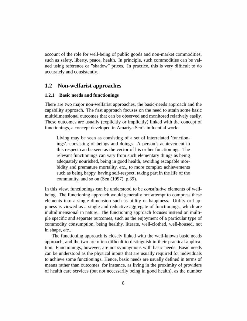
To illustrate the links between the main approaches to assessing poverty, considerFigure1. Figure1 shows in four quadrants the links between income, consump-tion of two commodities – transportation and clothing goods – and the function-ings associated to each of these two goods. The northeast quadrant shows a typicaltwo-good budget set for the two goodsT andC, namely, for transportation andclothing respectively, and with a budget constraintY 1. The curveU1 shows theutility indifference curve along which the consumer chooses his preferred com-modity bundle, which is here located at pointA.

11

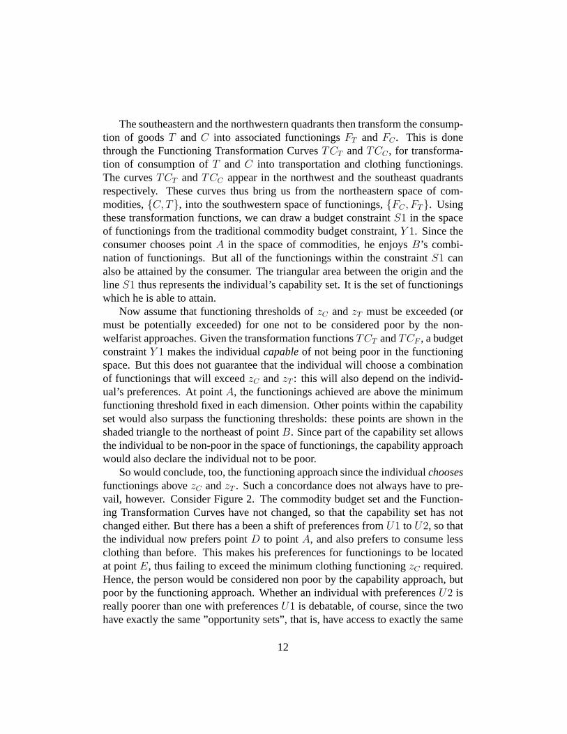
The southeastern and the northwestern quadrants then transform the consump-tion of goodsT and C into associated functioningsFT and FC . This is donethrough the Functioning Transformation CurvesTCT andTCC , for transforma-tion of consumption ofT andC into transportation and clothing functionings.The curvesTCT andTCC appear in the northwest and the southeast quadrantsrespectively. These curves thus bring us from the northeastern space of com-modities,C, T, into the southwestern space of functionings,FC , FT. Usingthese transformation functions, we can draw a budget constraintS1 in the spaceof functionings from the traditional commodity budget constraint,Y 1. Since theconsumer chooses pointA in the space of commodities, he enjoysB’s combi-nation of functionings. But all of the functionings within the constraintS1 canalso be attained by the consumer. The triangular area between the origin and theline S1 thus represents the individual’s capability set. It is the set of functioningswhich he is able to attain.

Now assume that functioning thresholds ofzC andzT must be exceeded (ormust be potentially exceeded) for one not to be considered poor by the non-welfarist approaches. Given the transformation functionsTCT andTCF , a budgetconstraintY 1 makes the individualcapableof not being poor in the functioningspace. But this does not guarantee that the individual will choose a combinationof functionings that will exceedzC andzT : this will also depend on the individ-ual’s preferences. At pointA, the functionings achieved are above the minimumfunctioning threshold fixed in each dimension. Other points within the capabilityset would also surpass the functioning thresholds: these points are shown in theshaded triangle to the northeast of pointB. Since part of the capability set allowsthe individual to be non-poor in the space of functionings, the capability approachwould also declare the individual not to be poor.

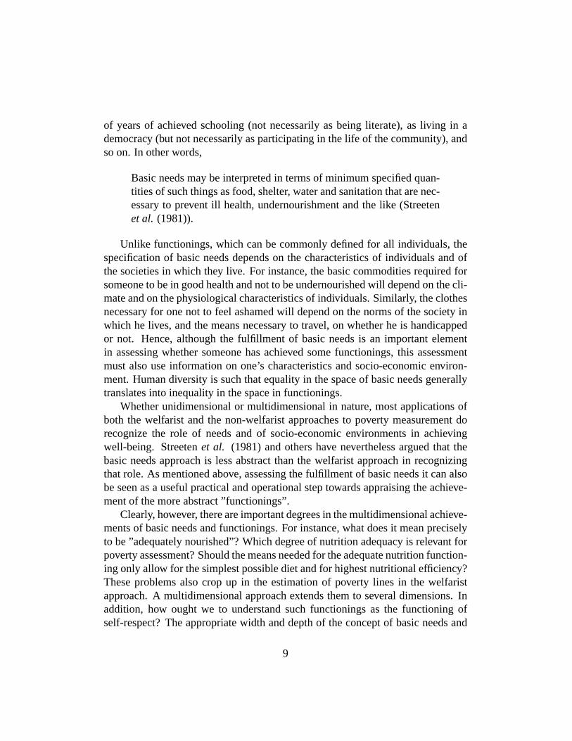
So would conclude, too, the functioning approach since the individualchoosesfunctionings abovezC andzT . Such a concordance does not always have to pre-vail, however. Consider Figure2. The commodity budget set and the Function-ing Transformation Curves have not changed, so that the capability set has notchanged either. But there has a been a shift of preferences fromU1 to U2, so thatthe individual now prefers pointD to pointA, and also prefers to consume lessclothing than before. This makes his preferences for functionings to be locatedat pointE, thus failing to exceed the minimum clothing functioningzC required.Hence, the person would be considered non poor by the capability approach, butpoor by the functioning approach. Whether an individual with preferencesU2 isreally poorer than one with preferencesU1 is debatable, of course, since the twohave exactly the same ”opportunity sets”, that is, have access to exactly the same

12

commodity and capability sets.An important message of the capability approach is that two persons with the

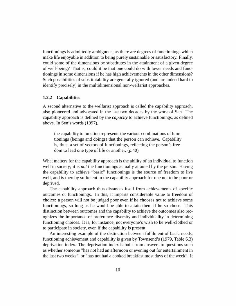
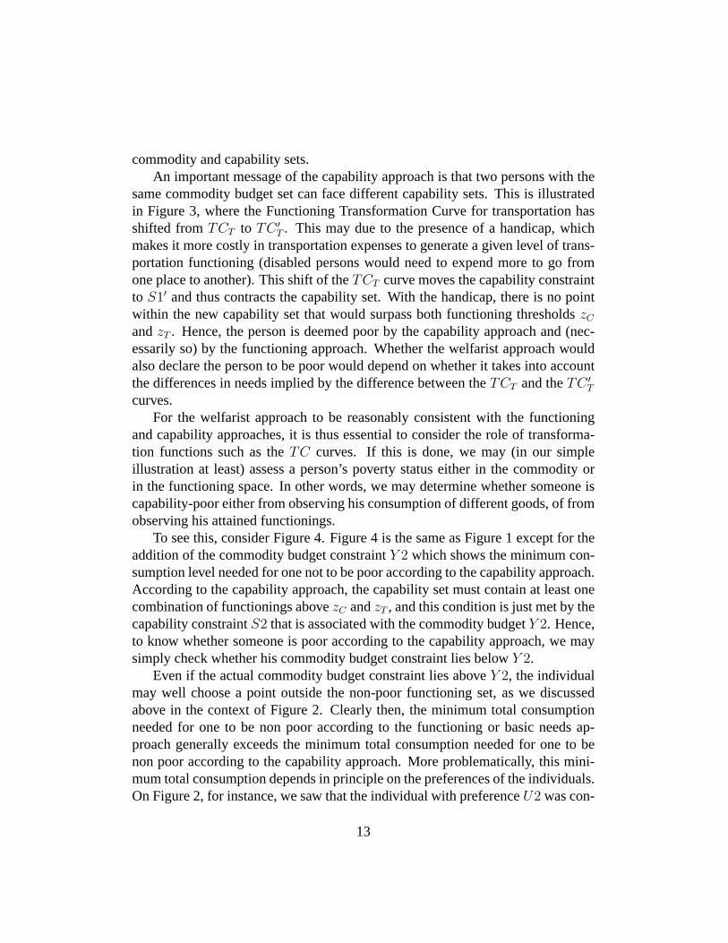
same commodity budget set can face different capability sets. This is illustratedin Figure3, where the Functioning Transformation Curve for transportation hasshifted fromTCT to TC ′

T . This may due to the presence of a handicap, whichmakes it more costly in transportation expenses to generate a given level of trans-portation functioning (disabled persons would need to expend more to go fromone place to another). This shift of theTCT curve moves the capability constraintto S1′ and thus contracts the capability set. With the handicap, there is no pointwithin the new capability set that would surpass both functioning thresholdszC

andzT . Hence, the person is deemed poor by the capability approach and (nec-essarily so) by the functioning approach. Whether the welfarist approach wouldalso declare the person to be poor would depend on whether it takes into accountthe differences in needs implied by the difference between theTCT and theTC ′

T

curves.For the welfarist approach to be reasonably consistent with the functioning

and capability approaches, it is thus essential to consider the role of transforma-tion functions such as theTC curves. If this is done, we may (in our simpleillustration at least) assess a person’s poverty status either in the commodity orin the functioning space. In other words, we may determine whether someone iscapability-poor either from observing his consumption of different goods, of fromobserving his attained functionings.

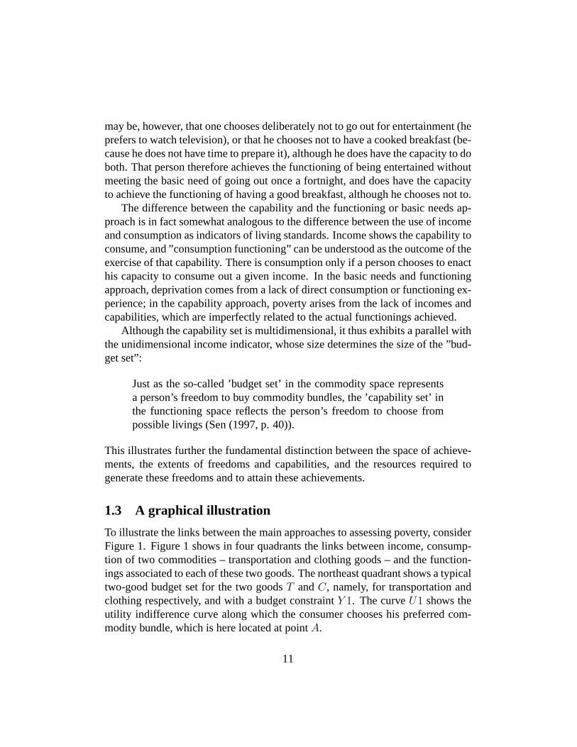
To see this, consider Figure4. Figure4 is the same as Figure1 except for theaddition of the commodity budget constraintY 2 which shows the minimum con-sumption level needed for one not to be poor according to the capability approach.According to the capability approach, the capability set must contain at least onecombination of functionings abovezC andzT , and this condition is just met by thecapability constraintS2 that is associated with the commodity budgetY 2. Hence,to know whether someone is poor according to the capability approach, we maysimply check whether his commodity budget constraint lies belowY 2.

Even if the actual commodity budget constraint lies aboveY 2, the individualmay well choose a point outside the non-poor functioning set, as we discussedabove in the context of Figure2. Clearly then, the minimum total consumptionneeded for one to be non poor according to the functioning or basic needs ap-proach generally exceeds the minimum total consumption needed for one to benon poor according to the capability approach. More problematically, this mini-mum total consumption depends in principle on the preferences of the individuals.On Figure2, for instance, we saw that the individual with preferenceU2 was con-

13

sidered poor by the functioning approach, although another individual with thesame budget and capability sets was considered non-poor by the same approach.

1.3.1 Exercises

1. Show on a figure such as Figure1 the impact of an increase in the price ofthe transportation commodity on the commodity and capability constraints.

2. On a figure such as Figure4, show the minimal commodity budget set thatensures that the person

(a) is just able to attain one of the two minimum levels of functioningszC

or zT ;

(b) chooses a combination of functionings such that one of them exceedsthe corresponding minimum level of functioningszC or zT ;

(c) is just able to attain both minimum levels of functioningszC andzT ;

(d) chooses a combination of functionings such that both exceed the cor-responding minimum level of functioningszC andzT .

(e) How do these four minimal commodity constraints compare to eachother?

1.4 Practical measurement difficulties

How are we to measure capabilities? Unless a person chooses to enact them in theform of functioning achievements, capabilities are not easily inferred. Achieve-ment of all basic functionings implies non-deprivation in the space of all capa-bilities; but a failure to achieve all basic functionings does not imply capabilitydeprivation. This makes the monitoring of functioning and basic needs an imper-fect tool for the assessment of capability deprivation. Besides, and as for basicneeds, there are clearly degrees of capabilities, some basic and some wider.

Non-welfarist (capability and basic needs) approaches to poverty measure-ment also suffer from some comparability problems. This is because they typi-cally generate multidimensional qualitative poverty criteria: their fulfilment typ-ically takes a simple dichotomic yes/no form. It is unlikely that true well-beingis such a dichotomic and discontinuous function of achievement and capabilities.Indeed, for most of the functionings assessed empirically, there are degrees ofachievement, such as for being healthy, literate, living without shame,etc... It

14

is important to take into account the varying degrees of poverty in assessing andcomparing the intensity of poverty. Besides, how should we assess adequately thedegree of poverty of someone who has the capability to achieve two functioningsout of three, but not the third? Is that person necessarily ”better off” than some-one who can achieve only one, or even none of them? Are all capabilities of equalimportance when we assess well-being?

The multidimensionality of the non-welfarist criteria also translates into greaterimplementation difficulties than for the usual proxy indicators of the welfarist ap-proach. In the welfarist approach, the size of the multidimensional budget is or-dinarily summarized by income or total consumption, which can be thought ofas a unidimensional indicator of freedom. A similar transformation into a uni-dimensional indicator is more difficult with the capability and basic needs ap-proaches. One possibility solution is to use ”efficiency-income units reflectingcommand over capabilities rather than command over goods and services” (Sen(1984, p.343), as we illustrated above when discussing Figure4. This, however,is practically difficult to do, since command over many capabilities is hard totranslate in terms of a single indicator, and since the ”budget units” are hardlycomparable across functionings such as well-nourishment, literacy, feeling self-respect, and taking part in the life of the community. On Figure4, anyone withan income belowY 2 would be judged capability-poor. But by how much doespoverty vary among these capability-poor? A natural measure would be a func-tion of the budget constraint. It is more difficult to make such measurements andcomparisons in the capability set.

Furthermore, although there are many different combinations of consump-tion and functionings that are compatible with a unidimensional money-metricpoverty threshold, the welfarist approach will generally not impose multidimen-sional thresholds. For instance, the welfarist approach will usually not require forone not to be poor that both food and non-food expenditures be larger than theirrespective food and non-food poverty lines. As indicated above, this simplifiesthe identification of the poor and the analysis of poverty.

15

2 Poverty measurement and public policy

The measurement of well-being and poverty plays a central role in the discussionof public policy and safety nets in particular. It is used, among other things, toidentify the poor and the non-poor, to design optimal poverty relief schemes, toestimate the errors of exclusion and inclusion in the set of the poor (also known asType I and Type II errors), and to assess the equity of poverty alleviation policy.How many of the poor, for instance, are excluded from safety net programmes? Isit the poorest of the poor who benefit most from public policy? Would a differentsort of poverty alleviation policy reduce deprivation further?

An important example of the central role of poverty measurement in the set-ting of public policy is the optimal selection of safety net targeting indicators. Thetheory of optimal targeting suggests that it will commonly be best to target indi-viduals on the basis of indicators that are as easily observable and as exogenousas possible, while being as correlated as possible with the true poverty status ofthe individuals. Indicators that are not readily observable by programme admin-istrators are of little practical value. Indicators that can be changed effortlesslyby individuals will be distorted by the presence of the programme, and will losetheir poverty-informative value. Whether available indicators are sufficiently cor-related with the deprivation of individuals in a population is given by a povertyprofile. The value of this profile will naturally be highly dependent on the partic-ular assumptions and the approach used to measure well-being and poverty.

Estimation of the errors of inclusion and exclusion of the poor is also a prod-uct of poverty profiling and measurement. These errors are central in the trade-offinvolved in choosing a wide coverage of the population – at relatively low ad-ministrative and efficiency costs – and a narrower coverage – with more generousforms of support for the fewer beneficiaries. However, as Van de Walle (1998)puts it, a narrower coverage of the population, with presumably smaller errors ofinclusion of the non-poor, does not inevitably lead to a more equitable treatmentof the poor:

Concentrating solely on errors of leakage to the non-poor can lead topolicies which have weak coverage of the poor (Van de Walle (1998,p.366)).

The terms of this trade-off are again given by a poverty assessment exercise.Another lesson of optimal redistribution theory is that it is ordinarily better to

transfer resources from groups with a high level of average well-being to those

16

with a lower one. What matters even more, however, is the distribution of well-being within each of the groups. For instance, equalising mean well-being acrossgroups does not usually eliminate poverty since there generally exist within-groupinequalities. Even within the richer group, for instance, there normally will befound some deprived individuals, whom a rich-to-poor cross-group redistributiveprocess would clearly not take out of poverty. The within- and between-groupdistribution of well-being that is required for devising an optimal redistributivescheme can be again revealed by a comprehensive poverty profile.

2.1 Welfarist and non-welfarist policy implications

The distinction between the welfarist and non-welfarist approaches to povertymeasurement often matters (implicitly or explicitly) for the assessment and thedesign of public policy. As described above, a welfarist approach holds that in-dividuals are the best judges of their own well-being. It would thus in principleavoid making appraisals of well-being that conflict with the poor’s views of theirown situation. A typical example of a welfarist public policy would be the provi-sion of adequate income-generating opportunities, leaving individuals decide andreveal whether these opportunities are utility maximising, keeping in mind theother non-income-generating opportunities that are open to them.

A non-welfarist policy analyst would argue, however, that raising income op-portunities is not necessarily the best policy option. This is partly because indi-viduals are not necessarily best left with their own resolutions, at least in an in-tertemporal setting, for their educational and environmental choices for instance.In other words, the poor’s short-run preoccupations may harm their long-termself-interest. For example, individuals may choose not to attend skill-enhancingprogrammes because they appear overly time costly in the short-run, and becausethey are not sufficiently convinced or aware of their long-term benefits.

Hence, if left to themselves, the poor will not necessarily spend their incomeincrease on functionings that basic-needs analysts would normally consider a pri-ority, such as good nutrition and health. Thus, fulfilling ”basic needs” cannotbe satisfied only by the generation of private income, but may require significantamounts of targeted and in-kind public expenditures on areas such as education,public health and the environment. This would be so even if the poor did notpresently believe that these areas were deserving of public expenditures. Further-more, social cohesion concerns are arguably not well addressed by the maximiza-tion of private utility, and raising income opportunities will not fundamentallysolve problems caused by adverse intra-household distributions of well-being, for

17

instance.An objection to the basic needs approach is that it is clearly paternalistic since

it supposes that it is in the absolute interests of all to meet a set of often arbi-trarily specified needs. Indeed, as emphasised above, non-welfarist approachesin general may use criteria for identifying and helping the poor that may con-flict with the poor’s views and utility maximizing options. For poverty alleviationpurposes, this could go as far as enforced enrolment in community developmentprogrammes. This would not only conflict with the preferences of the poor, butwould also clearly undermine their freedom to choose. Freedom to choose may,however, be one of the basic capabilities which contribute fundamentally to well-being.

A further example of the possible tension between welfarist and non-welfaristapproaches to public policy comes from optimal taxation theory, which is linkedto optimal poverty alleviation theory. In the tradition of classical microeconomics,which values leisure in the production and labour market decisions of individu-als, pure welfarists would incorporate the utility of leisure in the overall utilityfunction of workers, poor and non-poor alike. In its support to the poor, the gov-ernment would then take care of minimizing the distortion of their labor/leisurechoices so as not to create overly high ”deadweight losses”. Classical optimal tax-ation theory then shows that giving a positive weight to such things as labor/leisuredistortions suggests a generally lower benefit reduction rates on the income of thepoor than otherwise. Taking into account such abstract things is less typical ofthe basic needs and functioning approaches. Such approaches would, therefore,usually be less reluctant to target programme benefits more sharply on the poor,and exact steeper benefit reduction rates as income or well-being increases.

Relative to the pure welfarist approach, non-welfarist approaches are also typ-ically less reluctant to impose utility-decreasing (or ”workfare”) costs as side ef-fects of participation in poverty alleviation schemes. These side effects are in factoften observed in practice. For instance, it is well-known that income supportprogrammes frequently impose participation costs on benefit claimants. Theseare typically non-monetary costs. Such costs can be both physical and psycholog-ical: providing manual labor, spending energy, spending time away from home,sacrificing leisure and home production, finding information about application andeligibility conditions, corresponding and dealing with the benefit agency, queuing,keeping appointments, complying with application conditions, revealing personalinformation, feeling ”stigma” or a sense of guilt,etc...

Although non-monetary, these costs have a clear impact on participants’ netutility from participating in the programmes. When they are negatively correlated

18

with unobserved (or difficult to observe) entitlement indicators, they can provideself-selection mechanisms that enhance the efficiency of poverty alleviation pro-grammes, for welfarists and non-welfarists alike. One unfortunate effect of thesecosts is, however, that many truly-entitled and truly deserving individuals mayshy away from the programmes because of the costs they impose. Although pro-gramme participation could raise their income and consumption above a money-metric poverty line, some individuals will prefer not to participate, revealing thatthey find apparent poverty utility dominant over programme participation. Wel-farists would in principle take these costs into account when assessing the meritsof the programmes. Non-welfarists would typically not do so, and would thereforejudge the programmes more favorably.

The width of the definition of functionings is clearly also important for theassessment and the design of public policy. For instance, public spending oneducation is often promoted on the basis of its impact on productivity and growth.But education can also be seen as a means to attain the functioning of literacy andparticipation in the community. This provides an additional strong support forpublic expenditures on education. Analogous arguments also apply, for instance,to public expenditures on health, transportation, and the environment.

19

Part II

Measuring poverty and equity

20

3 Notation

In what follows in this book, we will denote living standards by the variabley. The indices we will use will sometimes require these living standards to bestrictly positive, and, for expositional simplicity, we will assume that this is al-ways the case. Strictly positive values ofy are required, for instance, for theWatts poverty index and for many of the decomposable inequality indices. It isof course reasonable to expect indicators of living standards such as monthly oryearly consumption to be strictly positive. This assumption is less natural for otherindicators, such as income, for which capital losses or retrospective tax paymentscan generate negative values.

Let p = F (y) be the proportion of individuals in the population who enjoya level of income that is less than or equal toy. F (y) is called the cumulativedistribution function (cdf) of the distribution of income; it is non-decreasing iny,and varies between 0 and 1, withF (0) = 0 andF (∞) = 1. For expositionalsimplicity, we may assume thatF (y) is continuously differentiable and strictlyincreasing iny (a reasonable assumption for large-population distributions of in-come). The density function, which is the first-order derivative of thecdf, is de-noted asf(y) = F ′(y) and is strictly positive sinceF (y) is assumed to be strictlyincreasing iny.

3.1 Continuous distributions

A useful tool throughout the analysis will be the concept of “quantiles”. Quantileswill help simplify greatly the exposition and the computation of several distribu-tive measures. They will also sometimes serve as direct tools to analyze and com-pare distributions of living standards (to check first-order dominance in the dualapproach for instance). The quantileQ(p) is defined asF (Q(p)) = p, or using theinverse distribution function, asQ(p) = F−1(p). Q(p) is thus the living standardlevel below which we find a proportionp of the population. Alternatively, it is theliving standard of that individual whose rank – or percentile – in the distributionis p. A proportionp of the population is poorer than he is; a proportion1 − p isricher than him.

This is illustrated in Figure14. The horizontal axis shows percentilesp of thepopulation. The quantilesQ(p) that correspond to differentp values are shownon the vertical axis. The larger the rankp, the higher the corresponding livingstandardQ(p). Alternatively, living standardsy appear on the vertical axis ofFigure14, and the proportion of individuals whose income is below or equal to

21

thosey are shown on the horizontal axis. At the maximum income level,ymax,that proportionF (ymax) equals 1. The median is given byQ(0.5), which is theliving standard which splits the distribution exactly in two halves.

We will define most of the distributive measures (indices and curves) in termsof integrals over a range of percentiles. This is a familiar procedure in the contextof continuous distributions. We will see below why this is also generally validin the context of discrete distributions, even though the use of summation signsis more familiar in that context. Using integrals will make the definitions andthe exposition simpler, and will help focus on what matters more, namely, theinterpretation and the use of the various indices and curves that we will consider.

The most common summary index of a distribution is its mean. Using integralsand quantiles, it is defined as:

µ =∫ 1

0Q(p)dp. (1)

µ is therefore simply the area underneath the quantile curve. This corresponds tothe grey area shown on Figure14. Since the horizontal axis varies uniformly from0 to 1,µ is also the average height of the quantile curveQ(p), and this is givenby µ on the vertical axis. As for most distributions of income, the one shownon Figure14 is skewed to the left, which gives rise to a meanµ that exceeds themedianQ(p). Said differently, the proportion of individuals underneath the mean,F (µ), exceeds one half.

For poverty comparisons, we will also need the concept of quantiles censoredat a poverty linez. These are denoted byQ∗(p; z) and defined as:

Q∗(p; z) = min(Q(p), z). (2)

Censored quantiles are therefore just the incomesQ(p) for those in poverty(below z) andz for those whose income exceeds the poverty line. This is illus-trated on Figure15, which is similar to Figure14. QuantilesQ(p) and censoredquantilesQ∗(p; z) are identical up top = F (z), or up toQ(p) = z. After thispoint, censored quantiles equalz and diverge from incomeQ(p).

Censoring income atz helps focus attention on poverty, since the precisevalue of those living standards that exceedz is irrelevant for poverty analysisand poverty comparisons (at least so long as we considerabsolutepoverty; moreon this later). The mean of the censored quantiles is denoted asµ∗(z):

22

µ∗(z) =∫ 1

0Q∗(p; z)dp. (3)

This is again the area underneath the curve of censored incomesQ∗(p; z). Thepoverty gap at percentilep, g(p; z), is the difference between the poverty line andthe censored quantile atp, or equivalently the shortfall (when applicable) of livingstandardQ(p) from the poverty line:

g(p; z) = z −Q∗(p; z) = max(z −Q(p), 0). (4)

When income atp exceeds the poverty line, the poverty gap equals zero. A short-fall g(q; z) at rankq is shown on Figure15 by the distance betweenz andQ(q).The larger one’s rankp in the distribution – the higher up in the distribution ofincome – the lower the poverty gapg(p; z). The proportion of individuals with apositive poverty gap is given byF (z) (see the Figure). The average poverty gapthen equalsµg(z):

µg(z) =∫ 1

0g(p; z)dp. (5)

µg(z) is the size of the area in grey shown in Figure15.

3.2 Discrete distributions

To see how to rewrite the above definitions using summation signs and discretedistributions, we need a little more notation. Say that we are interested in adistribution of n living standards. We first order then observations ofyi inincreasing values ofy, such thaty1 ≤ y2 ≤ y3 ≤ ... ≤ yn−1 ≤ yn. Wethen definen discrete quantiles of living standards asQ(pi) = yi, for pi =1/n, 2/n, 3/n, ..., (n− 1)/n, 1.

This is illustrated in Table?? wheren = 3 and where the incomes in increas-ing values are 10, 20 and 30. Figure13 graphs those quantiles as a function ofp.

The formulae for discrete distributions are then computed in practice by re-placing the integral sign in the continuous case by a summation sign, by summingacross all observed sample quantiles, and by dividing the sum by the number ofobservationsn. Thus, the meanµ of a discrete distribution can be expressed as:

23

µ =1

n

n∑

i=1

Q(pi). (6)

As indicated by equation (1), the mean of the discrete distribution of Table??,which is 20, is simply the integral of the quantile curve shown on Figure13. Inother words, it is the sum of the area of the three boxes each of length 1/3 that canbe found underneath the filled curve.

Discrete distributions are in fact what is always observed in samples and inreal-life populations of households or individuals, however large those samplesor populations may be. For clarity, we will mention from time to time how in-dices and curves can be estimated using the more familiar summation signs. Formore information, you can also consultDAD’s User Guidewhere the estimationformulae shown use summation signs and thus apply to discrete distributions.

24

4 The measurement of inequality and social welfare

4.1 Lorenz curves

The Lorenz curve has been for the several decades the most popular graphi-cal tool for visualizing and comparing the inequality in income. As we will see,it provides complete information on the whole distribution of income as a pro-portion of the mean. It therefore gives a more comprehensive description of therelative standards of living than any one of the traditional summary statistics ofdispersion can give, and it is also a better starting point when looking at the in-equality of income than the computation of the many inequality indices that havebeen proposed. As we will see, its popularity also comes from its use as a deviceto order distributions in terms of inequality, in such a way as to check whether theordering is necessarily the same for (and is therefore robust over) all inequalityindices within a large class of inequality indices. The Lorenz curve is defined asfollows:

L(p) =1

µ

∫ p

0Q(q)dq. (7)

The numerator shows the absolute contribution toper capita income of thebottomp proportion (the100p% poorest) of the population.µ is average income.L(p) thus indicates the cumulative percentage of total income held by a cumu-lative proportionp of the population, when individuals are ordered in increasingvalues of their income. For instance, ifL(0.5) = 0.3, then we know that the 50%poorest individuals hold 30% of the total income in the population.

A discrete formulation of the Lorenz curve is easily provided. Recall thatdiscrete incomeyi are ordered such thaty1 ≤ y2 ≤ ... ≤ yn, with percentilespi = i/n, for i = 1, ..., n. Fori = 1, ...n, the discrete Lorenz curve is then definedas:

L(pi = i/n) =1

nµ

i∑

j=1

Q (pj) . (8)

If needed, other values ofL(p) in (8) can be obtained by interpolation.The Lorenz curve has several interesting properties. It ranges from 0 atp =

0 to 1 atp = 1, since a proportionp = 1 of the population must also hold a

25

proportionL(p = 1) = 1 of the aggregate income. It is increasing asp increases,since more and more incomes are then added up. This is also seen by the fact thatthe derivative ofL(p) equalsQ(p)/µ,

dL(p)

dp=

Q(p)

µ. (9)

This is positive if income are stricly positive, as we have assumed. Hence byobserving the slope of the Lorenz curve at a particular value ofp, we also knowthep-quantile relative to the mean, or in other words, the standard of living of anindividual at rankp as a proportion of the overall mean standard of living. Theslope ofL(p) thus portrays the whole distribution of mean-normalised income.The Lorenz curve is also convex inp, since asp increases, the new incomes thatare being added up are greater than those that have already been counted. Math-ematically, a curve is convex when its second derivative is positive, and the morepositive that second derivative, the more convex is the curve. We can show thatthe second-order derivative of the Lorenz curve equals:

d2L(p)

dp2=

1

f(Q(p))(10)

which is positive. The larger the densityf(Q(p)) of income at a quantileQ(p),the more convex the Lorenx curve atL(p).

Some measures of central tendency can also be identified by a look at theLorenz curve. In particular, the median (as a proportion of the mean) is givenby Q(0.5)/µ, and thus by the slope of the Lorenz curve atp = 0.5. Since manydistributions of incomes are skewed to the right, the mean exceeds the medianand Q(p = 0.5)/µ will typically be less than one. The mean living standardin the population is found at the percentile at which the slope ofL(p) equals 1,that is, whereQ(p) = µ. Again, this percentile will often be larger than 0.5,namely, where the median living standard is located. The percentile of the mode(or modes) is whereL(p) is least convex, since by equation (10) this is where thedensityF (Q(p)) is highest.

If all had the same income, the Lorenz curve would equalp: population sharesand shares of total income would be identical. An important graphical element ofa Lorenz curve is thus its distance,p − L(p), from the line of perfect equality inincome.

Simple summary measures of inequality can already be obtained from thegraph of the Lorenz curve. The share in total income of the bottomp propor-tion of the population is given byL(p); the greater that share, the more equal is

26

the distribution of income. Analogously, the share in total income of the richestpproportion of the population is given by1−L(p); the greater that share, the moreunequal is the distribution of income. These two simple indices of inequality areoften used in the literature. An interesting but less well-known index of inequalityis given by the minimum (hypothetical) proportion of total income that the gov-ernment would need to reallocate across the population to achieve perfect equalityin income; this proportion is given by the maximum value ofp − L(p), which isattained where the slope ofL(p) is 1 (i.e., atL(p = F (µ))). It is therefore equalto F (µ) − LF (F (µ)) and is also called the Schutz coefficient. We will revert tothat coefficient later when we discuss relative poverty.

Mean-preserving equalising transfers of income are often call Pigou-Daltontransfers; in money-metric terms, they involve a marginal transfer of $1, say, froma richer to a poorer person, and they keep the mean of income constant. Allindices of inequality which do not increase (and sometimes fall) following anysuch equalising transfers are said to obey the Pigou-Dalton principle of transfers.These equalising transfers also have the consequence of moving the Lorenz curveunambiguously closer to the line of equality. Let the Lorenz curveLB(p) of adistributionB be everywhere above the Lorenz curveLA(p). We can thus thinkof B as having been obtained fromA through a series of equalising transfers,applied to the distributionA. Hence, inequality indices which obey the principleof transfers will unambiguously indicate more inequality inA than inB. We willcome back to this important link in the Section10on making robust comparisonsof inequality.

4.2 Gini indices

Compared to perfect equality, inequality thus removes a proportionp − L(p) oftotal income from the bottom100 · p% of the population. If we aggregate that“deficit” p − L(p) between population shares,p, and shares in income,L(p),across all values ofp between 0 and 1, we get half the well-known Gini index:

Gini index of inequality2

=∫ 1

0(p− L(p)) dp. (11)

The Gini index thus assumes that all “share deficits” acrossp are equally impor-tant. It thus computes the average distance between cumulated population sharesand cumulated shares in income. One can, however, also think of other weights toaggreate the distancep − L(p). The class oflinear inequality measures is given

27

by the use of rank- or percentile-dependent weights, sayκ(p), applied to that dis-tance. A popular one-parameter functional specification for such weights is givenby

κ(p; ρ) = ρ(ρ− 1)(1− p)(ρ−2) (12)

which depends on the value of a single “ethical” parameterρ which must begreater than 1 for the weightsκ(p; ρ) to be positive everywhere. The shape ofκ(p; ρ) is shown on Figure3 for three different values ofρ. The larger the valueof ρ, the larger the value ofκ(p; ρ) for smallp.

Using (12) gives what is called the class of S-Gini (or “Single-Parameter”Gini) inequality indices:

I(ρ) =∫ 1

0(p− L(p))κ(p; ρ)dp. (13)

Note that whenρ = 2, we have thatI(2) is the standard Gini index. This isbecauseκ(p; ρ = 2) ≡ 2, which then gives equal weight to all distancesp−L(p).When1 < ρ < 2, relatively more weight is given to the distances occurring atlarger values ofp, as shown by Figure3. Conversely, whenρ > 2, relatively moreweight is given to the distances occurring at lower values ofp. Changingρ thuschanges the “ethical” concern which we feel for the “shares deficits” at variouscumulative proportions of the population.

Let ω(p; ρ) be defined as follows:

ω(p; ρ) =∫ 1

pk(q, ρ)dq = ρ(1− p)ρ−1. (14)

Note thatω(p; ρ) > 0 and that∂ω(p; ρ)/∂p < 0 whenρ > 1. The shape ofω(p; ρ)is shown on Figure2 for ρ equal to 1.5, 2 and 3. Since

∫ 10 ω(p; ρ)dp = 1 for any

value ofρ, the area under each of the three curves on Figure2 equals 1 too.The functionsκ(p; ρ) andω(p; ρ) can be given an interpretation in terms of

densities of the poor, densities which will be useful to interpret some of the rela-tionships to be described below. Assume thatr individuals are randomly selectedfrom the population. The probability that the income ofall of theser individualswill exceedQ(p) is given by[1− F (Q(p))]r, and thus the probability of finding aliving standard belowQ(p) in such samples is1− [1− F (Q(p))]r = 1− [1− p]r.The density of the lowest rank of income in a sample ofr randomly selected in-come is the derivative of that probability with respect top, which is

r (1− p)r−1 . (15)

28

This helps us interpret the weightsκ(p; ρ) and ω(p; ρ). By equation (12),κ(p; ρ) is ρ times the density of the lowest living standard in a sample ofρ − 1randomly selected individuals; analogously, by equation (14), ω(p; ρ) is the den-sity of the lowest living standard in a sample ofρ randomly selected individuals.

Using (14) and by integration by parts of equation (13), we can then show that:

I(ρ) =1

µ

∫ 1

0(µ−Q(p))ω(p; ρ)dp. (16)

This says that the deviation of income from the mean is weighted by weightswhich fall with the ranks of individuals in the population. Since, in equation (16),I(ρ) is a (piece-wise) linear function of the incomeQ(p), it is a member of theclass of linear inequality measures, a feature which will prove useful in measuringprogressivity and vertical equity later.

We might be interested in determining the impact of some inequality-changingprocess on the inequality indices of type (16). One such process that can be han-dled nicely spreads income away from the mean by a proportional factorλ, andthus corresponds to some form of bi-polarization of incomes away from the mean(loosely speaking). This is equivalent to a process that adds(λ− 1) (Q(p) − µ)to Q(p), since

µ− (Q(p) + (λ− 1) (Q(p)− µ)) = λ (µ−Q(p)) . (17)

As can be checked from equation (16), this changesI(ρ) proportionally byλ,which also says that the elasticity ofI(ρ) with respect toλ, whenλ equals 1initially, is equal to 1 whatever the value of the parameterρ.

This bi-polarization away from the mean is also equivalent to a process thatincreases the distancep − L(p) by a factorλ. That this gives the same changein I(ρ) can be checked from equation (13). This bi-polarization process thusincreases the ”deficit”p − L(p) between population sharesp and income sharesL(p) by a constant factorλ across population shares or ranks. We will see laterhow this distance-increasing process leads to a nice illustration of the possibleimpact of changes in inequality on poverty.

As shown on Figure2, the larger the value ofρ, the greater the weight givento the deviation of low incomes from the mean. Whenρ becomes very large, theindex I(ρ) equals the proportional deviation from the mean of the lowest livingstandard. Whenρ = 1, the same weightω(p; ρ = 1) ≡ 1 is given to all devi-ations from the mean, which then makes the inequality indexI(ρ = 1) always

29

equal to 0, regardless of the distribution of income under consideration. Hence,ρ is a parameter of inequality aversion that determines our ethical concern for thedeviation of quantiles from the mean at various ranks in the population. In thissense, it is analogous to the parameterε of relative inequality aversion which wewill discuss below in the context of the Atkinson indices. For the standard Giniindex of inequality, we have thatρ = 2 and thus thatω(p; ρ = 2) = 2 · (1 − p);hence in assessing the standard Gini, the weight on the deviation of one’s livingstandard from the mean decreases linearly with one’s rank in the distribution ofincome. In a discrete formulation, the weightsω(p; ρ) take the form of:

ω(pi; ρ) =(n− i + 1)ρ − (n− i)ρ

nρ. (18)

The S-Gini indices of inequality have nice properties. First, they are graphi-cally easily interpreted as a weighted area underneath the Lorenz curve. Second,they range between 0 (when all incomes are equal to the mean or when the ethicalparameterρ is set to 1) and 1 (when incomes are concentrated in the hands of onlyone individual, or whenρ is large and the lowest living standard is close to 0).Since the Lorenz curve moves towardsp when a Pigou-Dalton equalising trans-fer is exerted, the value of the S-Gini indices also decreases with such transfers.Finally, the S-Gini indices can be shown to be equal to the following covarianceformula:

I(ρ) =−cov

(Q(p), ρ (1− p)(ρ−1)

)

µ(19)

which makes their computation simple using common spreadsheet or statisticalsoftwares. The traditional Gini is then simply:

I(ρ = 2) =2 cov(Q(p), p)

µ(20)

which is just a proportion of the covariance between incomes and their ranks.A further useful interpretive property of the standard Gini index is that it equals

half the mean-normalised average distance between all incomes:

I(ρ = 2) =

∫ 10

∫ 10 |Q(p)−Q(q)|dpdq

2 µ. (21)

30

Thus, if we find that the Gini index of a distribution of income equals 0.4, then weknow that the average distance between the incomes of that distribution is of theorder of 80% of the mean.

A final interesting interpretation of the Gini index is in terms of average rel-ative deprivation, which has been linked in the sociological and psychologicalliterature to subjective well-being, social protest and political unrest. For this, itis usual to quote from the classic work of Runciman (1966), who defines relativedeprivation as follows:

The magnitude of a relative deprivation is the extent of the differencebetween the desired situation and that of the person desiring it (as hesees it). (p.10)

Sen (1973), Yitzhaki(1979) and Hey and Lambert(1980) follow Runciman’slead to propose for each individual an indicator of relative deprivation which mea-sures the distance between his income and the income of all those relative to whomhe feels deprived. Thus, let the relative deprivation of an individual with incomeQ(p), when comparing himself to another individual with incomeQ(q), be givenby:

δ(p, q) =

0, if Q(p) ≥ Q(q)Q(q)−Q(p), if Q(p) < Q(q)

. (22)

The expected relative deprivation of an individual at rankp is thenδ(p):

δ(p) =∫ 1

0δ(p, q)dq (23)

which, we can show, can be computed asδ(p) = µ(1− L(p))−Q(p)(1− p). Aswe did for the “shares deficits” above, we can aggregate the relative deprivationat every percentilep by applying the weightsκ(p; ρ). We can show that this givesthe S-Gini index of inequality:

I(ρ) =1

ρ µ

∫ 1

0δ(p)κ(p; ρ)dp. (24)

Hence, the S-Gini indices are also an indicator of the average relative deprivationfelt in a population. By equations (12), (15) and (24), they equal the expectedrelative deprivation of the poorest individual in a sample ofρ − 1 randomly se-lected individuals. The greater the value ofρ, the more important is the relativedeprivation of the poorer in computingI(ρ).

31

4.3 Social welfare

We now introduce the concept of a social welfare function. Unlike the conceptof relative inequality, which considers incomes relative to the mean, the conceptof social welfare will allow us to measure and compare theabsoluteincomesof populations. We will see, however, that under some popular conditions onthe shape of social welfare functions, the measurement of inequality and socialwelfare can be nicely linked and integrated, and that the tools used for the twoconcepts are then similar.

The social welfare functions we will consider will take the form of:

W =∫ 1

0U(Q(p))ω(p)dp (25)

where for expositional simplicity we will restrictω(p) to be of the special formω(p; ρ) defined by equation (14). U(Q(p)) is a “utility function” of incomeQ(p).Social welfare is then the expected utility of the poorest individual in a sample of(ρ− 1) individuals.

The first requirement that we wish to impose on the form ofW is that it behomothetic. Homotheticity ofW is analogous to the requirement on consumerutility functions that expenditure shares of the different consumption goods beconstant as income increases, or the requirement on production functions thatthe ratio of the marginal products of inputs stays constant when all inputs aredoubled. For social welfare measurement, homotheticity implies that the ratio ofthe marginal social utilities of any two individuals in a population stays the sameeven when all incomes are doubled or halved1. For (25) to be homothetic, weneedU(Q(p)) to take the popular form ofU(Q(p); ε), where

U(Q(p); ε) =

Q(p)1−ε

(1−ε), when ε 6= 1

ln Q(p), when ε = 1. (26)

Hence,W in equation (25) will depend on the parametersρ and onε, and we willdenote this asW (ρ, ε).

Homotheticity of a social welfare function has an important advantage: thesocial welfare function can then be used to measure relative inequality, the mostcommon concept of inequality in the literature on the distribution of income. Tosee how this can be done, defineξ(ρ, ε) as the equally distributed living standardthat is equivalent, in terms of social welfare, to the actual distribution of income

1The marginal social utility of a living standardQ(p) is given by∂W/∂Q(p) = W (1).

32

(we will refer toξ as the EDE living standard).ξ(ρ, ε) is then implicitly definedas:

∫ 1

0U (ξ(ρ, ε); ε) ω(p; ρ) dp =

∫ 1

0U(Q(p); ε) ω(p; ρ) dp. (27)

Since∫ 10 ω(p; ρ)dp = 1, ξ(ρ, ε) is such that:

U (ξ(ρ, ε); ε) =∫ 1

0U(Q(p); ε)ω(p; ρ)dp (28)

or, alternatively:

ξ(ρ, ε) = U−1ε

(∫ 1

0Uε(Q(p))ω(p; ρ)dp

)= U−1

ε (W (ρ, ε)) (29)

whereU−1ε (·) is the inverse utility function:

U−1ε (x) =

(1− ε)s

11−ε , when ε 6= 1,

exp (x) , when ε = 1,. (30)

The index of inequalityI corresponding to the social welfare functionW is thendefined as the distance between the EDE living standard and mean income, as aproportion of mean income:

I =µ− ξ

µ= 1− ξ

µ. (31)

When using the specific formsW (ρ, ε) andξ(ρ, ε), this givesI(ρ, ε).Clearly, then, the EDE living standard is a simple function of average living

standard and inequality in its distribution, withξ = µ · (1 − I). Compare to theW , ξ also has the advantage of being money metric and thus of being easily un-derstood and compared to other economic indicators that can also be expressed inmoney-metric terms. To increase social welfare, we can either try to increaseµ,or increase equality of income1− I by decreasing inequalityI. Two distributionsof income can display the same social welfare even with different average incomeif these differences are offset by differences in inequality. This is shown in Figure23, starting initially with two different levels of mean incomeµ0 andµ1 and zeroinequality. We then have thatξ = µ0 andξ = µ1. To preserve the same level ofsocial welfare in the presence of inequality, mean income must be higher: this is

33

shown by the positive slope of the constantξ functions. Furthermore, as inequal-ity becomes large, further increases inI must be matched by higher and higherincreases in mean income for social welfare not to fall.

Defined as in (31), inequality has an interesting interpretation: it measures thedifference between the mean level of actual income and the (lower) level neededinstead to achieve the same level of social welfare when income is distributedequally across the population. This difference being expressed as a proportion ofmean income,I thus shows theper capitaproportion of income that is wastedin social terms because of its unequal distribution. Society as a whole would bejust as well-off with an equal distribution of a proportion of just1− I of the totalactual income.I can thus be interpreted as a money-metric indicator of the socialcost of inequality.

Let a distributionA of income just be a proportional re-scaling of a distributionB. In other words, for a constantλ > 0, we have thatQA(p) = λQB(p) for all p.If the social welfare function used for the computation ofI is homothetic, it mustbe thatIA = IB. This is illustrated in Figure20 for the case of two incomesyA

1

andyA2 for the case of an initial distributionA andyB

1 andyB2 for a ”scaled-up”

distributionB. Social welfare inA is given byWA. The social indifference curveWA shown in Figure20also depicts the many other combinations of incomes thatwould yield the same level of social welfare. One of these combinations, at pointF , corresponds to a situation of equality of income where both individuals enjoyξA. ξA is therefore the equally distributed living standard that is socially equivalentto the distribution(yA

1 , yA2 ).

The average living standard inA is given byµA, which is pointG in Figure20. Hence two distributions of income, one made of the vector(yA

1 , yA2 ) and the

other of the vector(ξA, ξA), generate the same level of social welfare, the firstwith an unequally distributed average living standardµA and the other with anequally distributed average living standardξA. Hence, the distance between pointF and pointG in Figure20 can be understood as the ”cost of inequality” in thedistributionA of income. Taking that distance as a proportion ofµA (see equation(31)) gives the index of inequality in the distributionA.

The fact thatyA1 = λyB

1 andyA2 = λyB

2 for the sameλ can be seen from thefact that the two vectors of income lie along the same ray from the origin. If thefunction W is homothetic, then inequality inA must be the same as inequalityin B. In other words, the distance between pointsD andE as a proportion ofthe distanceOE must be the same as the distance between pointsF andG as aproportion of the distanceOG.

34

4.3.1 Atkinson indices

Two special cases ofW (ρ, ε) are of particular interest in assessing social welfareand relative inequality. The first is when the rank of income is not important incomputing social welfare: this is obtained whenρ = 1, and it yields the well-known Atkinson additive social welfare function,W (ε):

W (ε) = W (ρ = 1, ε) =∫ 1

0U (Q(p); ε)) dp. (32)

The Atkinson social welfare function has often been interpreted as a utilitariansocial welfare function, whereU(Q(p); ε) is an individual utility function dis-playing decreasing marginal utilities of income, or whereU(Q(p); ε) correspondsto a concave social evaluation of a concave individual utility of income. It can beargued, however, that “it is fairly restrictive to think of social welfare as a sumof individual welfare components”, and that one might feel that “the social valueof the welfare of individuals should depend crucially on the levels of welfare (orincomes) of others” (Sen (1973, p.30 and 41). The unrestricted formW (ρ, ε) al-lows for such interdependence and is therefore more flexible than the Atkinsonadditive formulation. In the light of the above, we can also interpretW (ρ, ε) asthe expected utility of the poorest individual in a group ofρ randomly selectedindividuals. This interpretation of the social evaluation functionW (ρ, ε) confirmswhy it is not additive or separable in individual welfare: the social welfare weighton individual utility U(Q(p); ε) depends on the rankp of the individual in thewhole distribution of income.

Figure21shows the shape of the utility functionsU (y; ε)) for different valuesof ε2. Incomes are shown on the horizontal axis as a proportion of their mean, andutility U (y; ε)) can be read on the vertical axis. A normalizationU (µ; ε)) = 1has been applied for graphical convenience. Although for all values ofε, theslope ofU (y; ε)) is positive, it is obviously not always the same across all valuesof y. This is made more explicit on Figure22 which shows the marginal socialutility of incomeU (1) (y; ε)) for different values ofε. Again, a normalization ofU (1) (µ; ε)) = 1 was made. Forε = 0, the marginal social utility is constant:increasing by a given amount a poor person’s living standard has the same socialwelfare impact as increasing by the same amount a richer person’s living standard.For ε > 0, however, increasing the poor’s income is socially more desirable than

2This is drawn from Cowell ???.

35

increasing the rich’s. The larger the value ofε, the faster the marginal social utilityfalls with y.

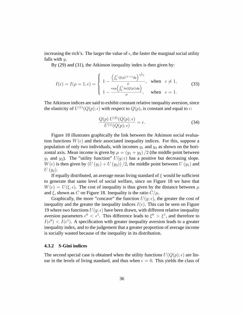
By (29) and (31), the Atkinson inequality index is then given by:

I(ε) = I(ρ = 1, ε) =

1−(∫ 1

0Q(p)(1−ε)dp

) 11−ε

µ, when ε 6= 1,

1−exp

(∫ 1

0ln(Q(p))dp

)

µ, when ε = 1.

(33)

The Atkinson indices are said to exhibit constant relative inequality aversion, sincethe elasticity ofU (1)(Q(p); ε) with respect toQ(p), is constant and equal toε:

Q(p) U (2)(Q(p); ε)

U (1)(Q(p); ε)= ε. (34)

Figure18 illustrates graphically the link between the Atkinson social evalua-tion functionsW (ε) and their associated inequality indices. For this, suppose apopulation of only two individuals, with incomesy1 andy2 as shown on the hori-zontal axis. Mean income is given byµ = (y1 + y2) /2 (the middle point betweeny1 and y2). The ”utility function” U(y; ε) has a positive but decreasing slope.W (ε) is then given by(U (y1) + U (y2)) /2, the middle point betweenU (y1) andU (y2).

If equally distributed, an average mean living standard ofξ would be sufficientto generate that same level of social welfare, since on Figure18 we have thatW (ε) = U(ξ, ε). The cost of inequality is thus given by the distance betweenµandξ, shown asC on Figure18. Inequality is the ratioC/µ.

Graphically, the more ”concave” the functionU(y; ε), the greater the cost ofinequality and the greater the inequality indicesI(ε). This can be seen on Figure19where two functionsU(y; ε) have been drawn, with different relative inequalityaversion parametersε0 < ε1. This difference leads toξ0 > ξ1, and therefore toI(ε0) < I(ε1). A specification with greater inequality aversion leads to a greaterinequality index, and to the judgement that a greater proportion of average incomeis socially wasted because of the inequality in its distribution.

4.3.2 S-Gini indices

The second special case is obtained when the utility functionsU(Q(p); ε) are lin-ear in the levels of living standard, and thus whenε = 0. This yields the class of

36

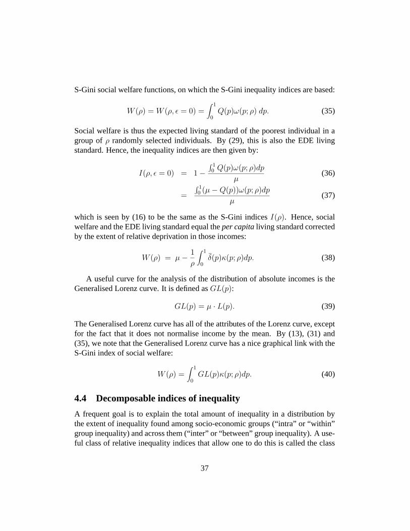
S-Gini social welfare functions, on which the S-Gini inequality indices are based:

W (ρ) = W (ρ, ε = 0) =∫ 1

0Q(p)ω(p; ρ) dp. (35)

Social welfare is thus the expected living standard of the poorest individual in agroup ofρ randomly selected individuals. By (29), this is also the EDE livingstandard. Hence, the inequality indices are then given by:

I(ρ, ε = 0) = 1−∫ 10 Q(p)ω(p; ρ)dp

µ(36)

=

∫ 10 (µ−Q(p))ω(p; ρ)dp

µ(37)

which is seen by (16) to be the same as the S-Gini indicesI(ρ). Hence, socialwelfare and the EDE living standard equal theper capitaliving standard correctedby the extent of relative deprivation in those incomes:

W (ρ) = µ− 1

ρ

∫ 1

0δ(p)κ(p; ρ)dp. (38)

A useful curve for the analysis of the distribution of absolute incomes is theGeneralised Lorenz curve. It is defined asGL(p):

GL(p) = µ · L(p). (39)

The Generalised Lorenz curve has all of the attributes of the Lorenz curve, exceptfor the fact that it does not normalise income by the mean. By (13), (31) and(35), we note that the Generalised Lorenz curve has a nice graphical link with theS-Gini index of social welfare:

W (ρ) =∫ 1

0GL(p)κ(p; ρ)dp. (40)

4.4 Decomposable indices of inequality

A frequent goal is to explain the total amount of inequality in a distribution bythe extent of inequality found among socio-economic groups (“intra” or “within”group inequality) and across them (“inter” or “between” group inequality). A use-ful class of relative inequality indices that allow one to do this is called the class

37

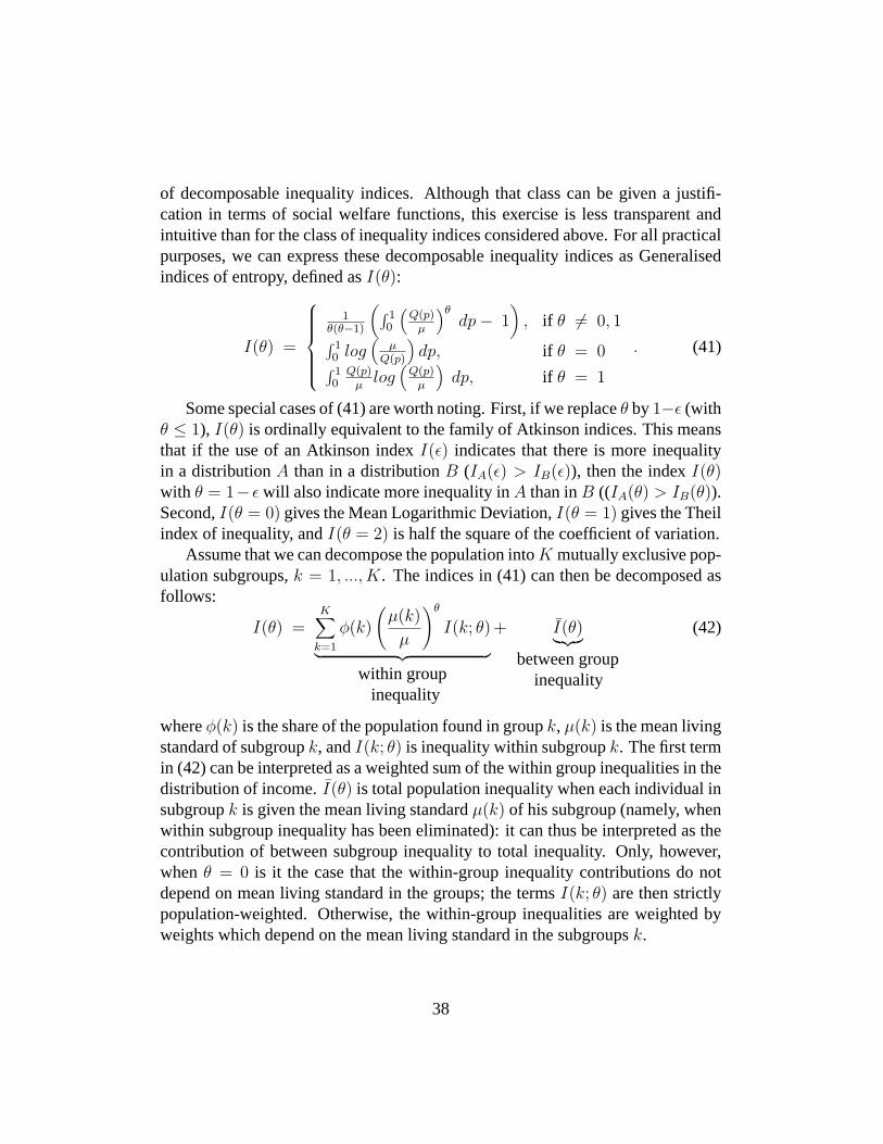
of decomposable inequality indices. Although that class can be given a justifi-cation in terms of social welfare functions, this exercise is less transparent andintuitive than for the class of inequality indices considered above. For all practicalpurposes, we can express these decomposable inequality indices as Generalisedindices of entropy, defined asI(θ):

I(θ) =

1θ(θ−1)

(∫ 10

(Q(p)

µ

)θdp− 1

), if θ 6= 0, 1

∫ 10 log

(µ

Q(p)

)dp, if θ = 0

∫ 10

Q(p)µ

log(

Q(p)µ

)dp, if θ = 1

. (41)

Some special cases of (41) are worth noting. First, if we replaceθ by1−ε (withθ ≤ 1), I(θ) is ordinally equivalent to the family of Atkinson indices. This meansthat if the use of an Atkinson indexI(ε) indicates that there is more inequalityin a distributionA than in a distributionB (IA(ε) > IB(ε)), then the indexI(θ)with θ = 1− ε will also indicate more inequality inA than inB ((IA(θ) > IB(θ)).Second,I(θ = 0) gives the Mean Logarithmic Deviation,I(θ = 1) gives the Theilindex of inequality, andI(θ = 2) is half the square of the coefficient of variation.

Assume that we can decompose the population intoK mutually exclusive pop-ulation subgroups,k = 1, ..., K. The indices in (41) can then be decomposed asfollows:

I(θ) =K∑

k=1

φ(k)

(µ(k)

µ

)θ

I(k; θ)

︸ ︷︷ ︸within group

inequality

+ I(θ)︸ ︷︷ ︸between group

inequality

(42)

whereφ(k) is the share of the population found in groupk, µ(k) is the mean livingstandard of subgroupk, andI(k; θ) is inequality within subgroupk. The first termin (42) can be interpreted as a weighted sum of the within group inequalities in thedistribution of income.I(θ) is total population inequality when each individual insubgroupk is given the mean living standardµ(k) of his subgroup (namely, whenwithin subgroup inequality has been eliminated): it can thus be interpreted as thecontribution of between subgroup inequality to total inequality. Only, however,whenθ = 0 is it the case that the within-group inequality contributions do notdepend on mean living standard in the groups; the termsI(k; θ) are then strictlypopulation-weighted. Otherwise, the within-group inequalities are weighted byweights which depend on the mean living standard in the subgroupsk.

38

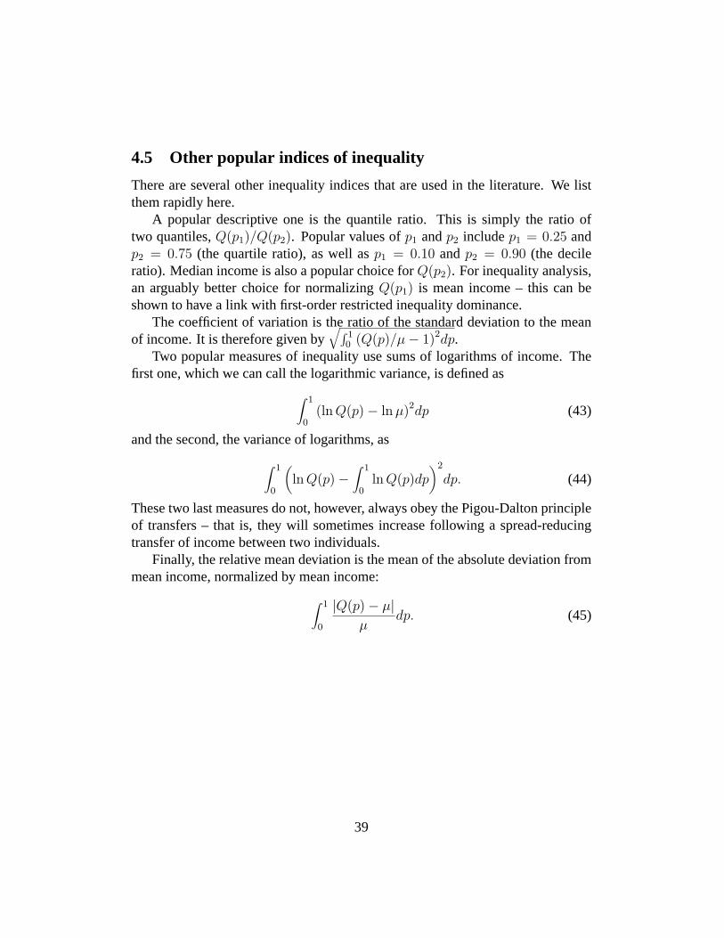
4.5 Other popular indices of inequality

There are several other inequality indices that are used in the literature. We listthem rapidly here.

A popular descriptive one is the quantile ratio. This is simply the ratio oftwo quantiles,Q(p1)/Q(p2). Popular values ofp1 andp2 includep1 = 0.25 andp2 = 0.75 (the quartile ratio), as well asp1 = 0.10 andp2 = 0.90 (the decileratio). Median income is also a popular choice forQ(p2). For inequality analysis,an arguably better choice for normalizingQ(p1) is mean income – this can beshown to have a link with first-order restricted inequality dominance.

The coefficient of variation is the ratio of the standard deviation to the meanof income. It is therefore given by

√∫ 10 (Q(p)/µ− 1)2dp.

Two popular measures of inequality use sums of logarithms of income. Thefirst one, which we can call the logarithmic variance, is defined as

∫ 1

0(ln Q(p)− ln µ)2dp (43)

and the second, the variance of logarithms, as

∫ 1

0

(ln Q(p)−

∫ 1

0ln Q(p)dp

)2

dp. (44)

These two last measures do not, however, always obey the Pigou-Dalton principleof transfers – that is, they will sometimes increase following a spread-reducingtransfer of income between two individuals.

Finally, the relative mean deviation is the mean of the absolute deviation frommean income, normalized by mean income:

∫ 1

0

|Q(p)− µ|µ

dp. (45)

39

5 Aggregating and comparing poverty

Making poverty comparisons is essential to determine whether poverty has changedacross time, or how it compares across countries, regions, or socio-economicgroups. Poverty comparisons are also essential for designing public policy, and forassessing its effects on poverty. They may be used, for instance, to judge whetherand by how much a public safety net reduces poverty and whether a reform to itsstructure could be alleviating poverty further.

5.1 Cardinal versus ordinal comparisons

There are two types of poverty comparisons, cardinal and ordinal. Cardinal povertycomparisons simply involve differences in numerical poverty estimates. Numeri-cal poverty estimates attach a single number to the extent of poverty in a popula-tion, for instance, 40% or $200 per capita. These estimates are valuable when aprecise number must be attached to the extent of poverty in a distribution of well-being. Cardinal poverty estimates require specific and precise assumptions, suchas the nature of the poverty index, the definition of the indicator of well-being,the value of the poverty line, and how that poverty line varies exactly acrosshousehold types, regions and time. Once this information is provided, cardinalpoverty estimates can tell, for instance, that 30% of the individuals in a popula-tion used to have their consumption lie underneath their poverty line, but that arecently-introduced public safety net has decreased that proportion to 25%. Car-dinal poverty estimates can also be used to carry out a money-metric cost-benefitanalysis of the effects of safety nets. Thus, if the above safety net involved yearlyexpenditures of $ 500 million, then we would know immediately that a 1% fall inthe proportion of the poor would seem to cost the government on average $ 100million. That amount could then be compared to the poverty alleviation cost ofother forms of government policy.

The main advantage of cardinal poverty estimates is their ease of communi-cation, their ease of manipulation, and their (apparent) lack of ambiguity. Gov-ernment officials and the media often want the results of poverty comparisons tobe produced in straightforward and precise terms, and can feel annoyed when thisis not possible. Cardinal poverty estimates are, however, necessarily (and oftenhighly) sensitive to the choice of a number of arbitrary measurement assump-tions. It is clear, for example, that choosing a different poverty line will almostalways change the estimated numerical value of any index of poverty. The elas-ticity of the poverty headcount index to the poverty line is, for example, almost

40

always significantly larger than 1. This implies that a variation of 10% in thepoverty line will change by more than 10% the estimated proportion of the poorin the population; this is a substantial impact for those interested in poverty alle-viation, especially since poverty lines are rarely convincingly bounded within anarrow confidence interval. Another source of numerical variability comes fromthe choice of the form of the poverty index. Many procedures have been proposedto aggregate numerically the poverty of individuals. Depending on the chosenprocedure, numerical estimates of poverty will appear large or low. As we willsee later, for instance, the estimation of a ”socially representative poverty gap”will rest particularly on the weight given to the more deprived among the poor.There is little objective guidance in choosing that weight; the greater that weight,however, the greater the estimated socially representative poverty gap, and thegreater the numerical estimate of poverty.

We will return to ordinal comparisons of poverty later. For now, we considerthe construction of aggregate cardinal poverty indices.

5.2 Aggregating poverty

Two approaches have been used to devise cardinal indices of poverty. The firstuses the concept of the equally distributed equivalent (EDE) living standard ofa society where incomes have been censored at the poverty line, and comparesit to the poverty line. The second combines income and the poverty line intopoverty gaps, and aggregates them in social-welfare like functions to assess over-all poverty. We look at these two approaches in turn.

5.2.1 The EDE approach

For the EDE approach to building poverty indices, we simply use the distribu-tion of incomeQ(p). Since, for poverty comparisons, we want to focus on thoseincomes that fall below the poverty line (the “focus axiom”), the incomesQ(p)are censored at the poverty linez, to giveQ∗(p; z). The censored incomes arethen aggregated using one of the many social welfare functions that have beenproposed in the literature. A poverty index is obtained by taking the differencebetween the poverty line and the EDE living standard. For instance, for the so-cial welfare functions proposed in section4.3, this leads to the following class ofpoverty indices:

P (z; ρ, ε) = z − ξ∗(z; ρ, ε) (46)

41

whereξ∗(ρ, ε) is the EDE living standard of the distribution of censored incomeQ∗(p; z) and where we needρ ≥ 1 and ε ≥ 0 for the Pigou-Dalton transferprinciple not to be violated.P (z; ρ, ε) can then be interpreted as the “sociallyrepresentative” or EDE poverty gap.

Examples of such poverty indices include a transformation of the Clark, Hem-ming and Ulph’s (CHU) second class of poverty indices, given byP (z; ε) =P (z; ρ = 1, ε):

P (z; ε) =

z −(∫ 1

0 Q∗(p; z)(1−ε)dp) 1

1−ε , when ε 6= 1,

z − exp(∫ 1

0 ln(Q∗(p; z))dp), when ε = 1.

(47)

The CHU indices are then obviously closely related to the Atkinson social welfarefunctions and inequality indices. Whenε = 1, the CHU poverty index is also theEDE poverty gap corresponding to the Watts poverty index, which is defined as:

PW (z) =∫ 1

0ln

(z

Q∗(p; z)

)dp. (48)

For 0 ≤ ε ≤ 1, the CHU indices also correspond to the EDE poverty gap of theclass of poverty indices proposed by Chakravarty:

PC(z; ε) = 1−∫ 1

0

(Q∗(p; z)

z

)1−ε

dp, 0 ≤ ε ≤ 1. (49)

Moreover, if we imposeε = 0 on the class of indices defined in (46), we obtainthe class of S-Gini indices of poverty:

P (z; ρ) = P (z; ρ, ε = 0) = z −∫ 1

0Q∗(p; z)ω(p; ρ)dp. (50)

P (z; ρ = 2) is known as the Thon-Chakravarty-Shorrocks index of poverty (it canalso be more simply referred to as the “Gini” index of poverty).

5.2.2 The poverty gap approach

The second approach reduces the information necessary to aggregate poverty tothe distribution of poverty gaps,g(p; z) = z − Q∗(p; z). Once this distribution isknown, no other use of the poverty line is allowed or needed in the aggregation ofpoverty. Because of this, the poverty gap approach to constructing poverty indices

42

is more restrictive and puts more structure on the shape of the allowable povertyindices than the previous EDE approach. After the distribution of poverty gapshas been computed, we may use aggregating functions analogous to those usedin section4.3 for the analysis of social welfare . Unlike social welfare functions,however, where we normally wish an increase in someone’s living standard to in-crease social welfare, we would normally wish the poverty indices to bedecreas-ing in poverty gaps. Further, whereas an equalizing Pigou-Dalton transfer wouldoften increase the value of a social welfare function, we would typically wish apoverty index to decrease when such an equalizing transfer of income takes placeamong the poor.

A popular class of poverty gap indices that can obey these axioms is knownas the Foster-Greer-Thorbecke (FGT) class. It differentiates its members using anethical parameterα ≥ 0 and is generally defined as

P (z; α) =∫ 1

0

(g(p; z)

z

)α

dp (51)

for the normalized FGT poverty indices and as

P (z; α) =∫ 1

0g(p; z)αdp (52)

for the un-normalized version (which can sometimes be more useful than the usualnormalized form). Note that poverty gap indices other than the FGT ones canalso be easily proposed, simply by using other aggregating functions of povertygaps that obey some of the desirable axioms (such as that of being increasing andconvex in poverty gaps) discussed in the literature.

Whenα = 0, the FGT index gives the simplest and most common example ofa poverty index. This is called the poverty headcount, and is simply the proportionof the poor (those with a positive poverty gap) in a population,F (z). The nextsimplest and most commonly used index,µg(z), is given by the average povertygap,P (z; α = 1), and is the average shortfall of income from the poverty line:

µg(z) = P (z; α = 1) =∫ 1

0g(p; z)dp. (53)

To see how to interpret the form of the FGT indices for general values ofα,consider Figure27. It shows the (absolute) contributions to total povertyP (z; α)of individuals at different ranksp. These contributions are given by(g(p; z)/z)α.For α = 0, the contribution is a constant 1 for the poor and 0 for the rich (those

43

whose rank exceedsF (z) on the Figure, or equivalently whose incomeQ(p) ex-ceedsz). The headcount is then the area of the dotted rectangle on Figure27. Forα = 1, the contribution equals precisely the normalized poverty gap,g(p; z)/z.The normalized average poverty is then the area underneath theg(p; z)/z drawnon Figure27. The same reasoning is valid for higher values ofα. For instance,the absolute contribution toP (z; α = 3) of individuals at rankp is given by(g(p; z)/z)3 on Figure27.

Notwithstanding the above, interpreting the value of FGT indices forα 6= 0, 1can be problematic. We can easily comprehend what a proportion of the popula-tion in poverty or an average poverty gap signifies, but what, for instance, can asquared-poverty-gap index actually mean? And how to explain it to a governmentminister?... A further difficulty with such indices emerges from another look atFigure27, which suggests that the contribution of the poor (including the poorest)to total povertydecreaseswith α – the contribution curves(g(p)/z)α move downasα rises. This also implies that the normalized FGT indices necessarily fall asαincreases. This is paradoxical since it is often argued that the higher the value ofα, the greater the focus on those who suffer most ”severely” from poverty.

One partial solution to these interpretive problems is to switch one’s focusfrom theabsoluteto therelativecontribution to total FGT poverty of individualswith different poverty gaps. Such relative contribution is depicted on Figure28for α = 0, 1 and 2. It shows the ratio of the absolute contributionsg(p)α to totalpovertyP (z; α) (these ratios are the same for normalized and un-normalized FGTindices). Since we are graphing here relative contributions to total poverty, thearea underneath each of the three curves must in all cases equal 1.

For α = 0, each poor contributes relatively the same constant1/F (z) to thepoverty headcount. The poor’s relative contribution to the average poverty gapnaturally increases with their own poverty gap, as shown by the curveg(p)/P (z; α =1). That relative contribution equals 1 at those individuals whose own poverty gapis precisely equal to the average poverty gap. The rank of such individuals is givenby F (µg(z)), as also shown on Figure28. Thus, those located atp = F (µg(z))have a poverty gap that is representative of the average poverty gap in the popula-tion. Increasingα from 1 to 2 decreases the relative contribution of not-so-poor,but increases reciprocally the contribution of those with the highest poverty gaps.This is then consistent with the general opinion that, in the aggregation of poverty,higher values ofα put more emphasis on those who suffer most severely frompoverty – those with lower values ofp and higher values ofg(p; z).

Figure28 does not, however, solve the main interpretation problems associ-ated with the FGT indices. As mentioned above, explaining to non-technicians or

44

policymakers the practical meaning of FGT indices for general values ofα canprove hazardous since these indices are averages ofpowersof poverty gaps. Theyare also not money metric nor unit-free (except forα = 0 and 1). An anotheralready-mentioned difficulty is that the usual FGT indices will generally fall withan increase in the value of their poverty-severity parameter. A valuable and in-tuitive solution to these two problems is to transform the FGT indices into EDEpoverty gaps. An EDE poverty gap is that poverty gap which – if it were as-signed equally to all individuals – would yield the same aggregate index as thatwhich is currently observed. An EDE poverty gap can then be usefully be in-terpreted as a socially-representative poverty gap. This transformation providesa money-metric measure of poverty which can be usefully compared across dif-ferent poverty indices and/or across different values ofα. As we will see later,it also allows the analyst to determine the impact of poverty-gap inequality uponthe level of poverty. For the un-normalized FGT indices, the EDE poverty gap isgiven simply by (forα > 0)

ξg(z; α) = [P (z; α)]1/α . (54)

For the normalized FGT indices, it is justξg(z; α) = ξg(z; α)/z.

Figure29 shows such socially-representative poverty gapsξg(z; α) for differ-ent values ofα. In each case, we obtain a socially-weightedmoney-metricindica-tor of the distribution of deprivation in the population. This summary aggregateindicator can also be compared to the individual distribution of poverty, given bytheg(p; z) curve. Those whoseg(p; z) exceedsξg(z; α) experience more povertythan the social average. Those exactly atξg(z; α) are exactly representative ofthe socially-weighted average poverty gap. Those representative of populationpoverty are thus found at the rank given byF (ξg(z; α)), which is also shown onFigure29.

An important point to note is that an increase inα moves the socially-representativepoverty gap closer to that experienced by the poorest individuals. This is becausethat, contrary to the usual FGT indices,ξg(z; α + 1) ≥ ξg(z; α) for anyα > 0.Hence, we can interpret increases inα as increases in the relative weight givento the poorer in computing the socially-representative poverty gap. The larger thevalue ofα, the more important are the most severe cases of deprivation in drawingup a representative aggregate picture of poverty.

Note finally that, besides being already in an EDE poverty gap form, the S-Gini index of poverty also has the property of being a poverty gap index. Indeed,by (50), we have that:

45

P (z; ρ) =∫ 1

0g(p; z)ω(p; ρ)dp (55)

5.3 Group-decomposable poverty indices

Much of the literature on the construction of poverty indices has focussed onwhether indices are decomposable across population subgroups. This has led tothe identification of a subgroup of poverty indices known as the “class of decom-posable poverty indices”. These indices have the property of being expressibleas a weighted sum (more generally, as a separable function) of the same povertyindices assessed across population subgroups. They most commonly include theFGT and the Chakravarty classes of indices as well as the Watts index.

Let the population be divided intoK mutually exclusive population subgroups,whereφ(k) is the share of the population found in subgroupk. For the FGT index,we then have that:

P (z; α) =K∑

k

φ(k)P (k; z; α) (56)

whereP (k; z; α) is the FGT poverty index of subgroupk. The Watts and Chakravartyindices are expressible as a sum of the poverty indices of each subgroup in exactlythe same way as for the FGT indices in (56).

To illustrate the practical contents of this property, consider the following two-group (K = 2) example. Let the first group contain 40% of the total population,and let the poverty in group 1 be 0.8 and in group 2 be 0.4. Poverty in the totalpopulation is then a simple weighted mean of the group poverty, and is immedi-ately computable as0.4·0.8+0.6·0.4 = 0.56. Estimates of poverty in a populationcan then be constructed in a decentralized manner, community by community orregion by region, without a need for all micro data to be regrouped in one register.

Subgroup decomposability also implies that an improvement in one of thesubgroups will necessarily improve aggregate poverty if the living standards inthe other groups have not changed. It will further mean that the design of socialsafety nets and benefit targeting within any given group can be done independentlyof the distribution of income in the other groups. This enables targeting to be donein a decentralized manner: only the characteristics of a relevant population matterfor the exercise. If targeting succeeds in decreasing poverty at a local level, thenit must succeed also at the aggregate level.

46

Subgroup decomposability is therefore useful, although it is certainly not im-perative for poverty analysis. In particular, it must be admitted that it is not be-cause an index property facilitates poverty profiling and the analysis of the com-parative advantages of various forms of targeting that this property is ethicallyfine. Among other things, imposing the decomposability and additivity propertycan mean losing some important ethical aspects to the aggregation of poverty. Inthat context, Ravallion (1994) notes that when measuring poverty ”one possibleobjection to additivity is that it attaches no weight to one aspect of a poverty pro-file: the inequality between sub-groups in the extent of poverty”. This can be animportant flaw if considerations of between-group relative deprivation are signifi-cant.

5.4 Poverty and inequality

Expressing poverty indices in the form of EDE poverty gaps allows one to separatethe impact of the average level of poverty and of the inequality in income uponthe index of poverty. Letξg(z) be the EDE poverty gap, andΞg(z) be the cost ofinequality on the level of poverty. Then,

ξg(z)− µg(z) = Ξg(z). (57)

For instance, for the popular FGT indices, we have that:

Ξg(z; α) = ξg(z; α)− µg(z). (58)

Whenα = 1, the inequality of poverty gaps is not taken into account in computingpoverty, and thus the cost of inequality on poverty is nil:Ξg(z; α = 1) = 0. Forα > 1, Ξg(z; α) is positive, but for0 < α < 1, we have thatΞg(z, α) < 0 since(ceteris paribus) the greater the level of inequality, thelower the assessed level ofpoverty.ξg(z; α) andΞg(z; α) are both increasing inα: the larger the value ofα,the larger the cost of inequality in poverty gaps on the level of aggregate poverty.We can thus interpretα as a parameter of inequality aversion in measuring poverty.

A similar decomposition can be done using (46) and the EDE level of censoredincome. The EDE poverty gap corresponding to that approach is defined as

z − ξ∗(z; ρ, ε) = z − µ∗(z)(1− I∗(z; ρ, ε))= µg(z) + Ξ∗(z; ρ, ε)

(59)

whereΞ∗(z; ρ, ε) = µ∗(z) · I∗(z; ρ, ε) is the cost of inequality in censored incomeand whereI∗(z; ρ.ε) is the index of inequality in censored income.

47

5.5 Poverty curves

It is generally informative to portray the whole distribution of poverty gaps on asimple graph, in a way which shows both the incidence and the inequality of thedeprivation in income. Particularly useful are the poverty gap curves, which plotg(p; z) as a function ofp. The poverty gap curve shows the ”intensity of poverty”felt at each rank in the population. The curve naturally decreases with the rankpin the population, and reaches zero at the value ofp equal to the headcount ratio.The integral under the curve gives the average poverty gap, and its steepness, thedegree of inequality in the distribution of poverty gaps.

Another quantile-based curve that is graphically informative and that is usefulfor the measurement and comparison of poverty is called the Cumulative PovertyGap (CPG) curve (also sometimes referred to as the inverse generalized Lorenzcurve, the “TIP” curve, or the poverty profile curve). The CPG curve cumulatesthe poverty gaps of the bottomp proportion of the population. It is defined as:

G(p; z) =∫ p

0g(q; z)dq. (60)

A CPG curve is drawn on Figure5. The slope ofG(p; z) at a given valueof p shows the poverty gapg(p; z). Sinceg(p; z) is non-negative,G(p; z) isnon-decreasing.G(p = 1; z) equals the average poverty gapµg(z), and the per-centile at whichG(p; z) becomes horizontal (whereg(p; z) becomes zero) yieldsthe poverty headcount. Furthermore, the higher his rankp in the population, thericher is an individual, and therefore the lower is his poverty gap.G(p; z) is there-fore concave. Because of this, the CPG curve also enjoys for poverty comparisonsthe same descriptive interest as the Lorenz and Generalized Lorenz curves for in-equality and social welfare analysis. The distance ofG(p; z) from the line ofperfect equality of poverty gaps (namely, the line 0B in Figure5) displays theinequality of poverty gaps among the population. The distance ofG(p; z) fromthe line of perfect equality of poverty gapsamong the poor(namely, the line 0Ain Figure5) displays the inequality of poverty gaps among the poor. Finally, theconcavity ofG(p; z) shows the density of poverty gaps atp.

5.6 S-Gini poverty indices

When weighted byκ(p; ρ), the area underneath the CPG curve generates the classof S-Gini poverty indices:

48

P (z; ρ) =∫ 1

0G(p; z)κ(p; ρ)dp. (61)

P (z; ρ = 1) equals the average poverty gap,µg(z), P (z; ρ = 2) is the povertyindex corresponding to the standard Gini index of inequality, and the well knownSen index of poverty is given by:

P (z; ρ = 2)

F (z) · z . (62)

An interesting feature of theP (z; ρ) indices is their link with absolute andrelative deprivation. Let absolute deprivation,AD(z), be given by the averageabsolute shortfall from the poverty line,µg(z). Relative deprivation in censoredincome at percentilep is given by :

δ∗(p; z) =∫ 1

p(Q∗(q; z)−Q∗(p; z))dq. (63)

Average relative deprivation across the whole population is thus :

RD(z; ρ) =∫ 1

0δ∗(p; z)κ(p; ρ)dp. (64)

We can then show that:

P (z; ρ) = AD(z) + RD(z, ρ). (65)

The larger the value ofρ, the larger is relative deprivation, and the larger isP (z; ρ)and the contribution of relative deprivation and inequality in assessing poverty.This is an alternative way of expressing the impact of inequality upon poverty.

5.7 The normalization of poverty indices

Most of the poverty indices discussed above have initially been introduced in theliterature in a normalized form, that is, by dividing censored income and povertygaps by the poverty line. The FGT indices, for instance, are generally expressedas:

P (z; α) =∫ 1

0

(z −Q∗(p)

z

)α

dp (66)

(see (51). The normalization of poverty indices will make no substantial differ-ence and little expositional difference for poverty analysis when the distributions

49

of income being compared have identical poverty lines. Normalizing poverty in-dices by the poverty line will make the EDE poverty gap lie between 0 and 1, willmake poverty indices insensitive to and independent of the monetary units (e.g.,dollars or cents) used in assessing income, and will make the indices invariant toan equi-proportionate change in all incomes and in the poverty line. This is par-ticularly useful if the poverty lines computed are to be interpreted as price indices,and used to enable comparisons of nominal income across time and areas (priceindices are used to convert nominal incomes into base-year real incomes). We canthus refer to normalized poverty indices as “relative poverty indices”. FGT andother poverty gap indices that are not normalized can be called “absolute” povertyindices since equal additions to all incomes and to the poverty line will not affecttheir value.

When poverty lines are different across distributions, and when they act asmore than simple price indices, the normalization of poverty indices by thesepoverty lines can, however, be problematic, and is surely open to criticism. This isthe case for instance when we are interested in comparing the absolute shortfallsof “real” income from a “real” poverty line, when these real poverty lines varyacross populations or population subgroups. Examples can arise,inter alia, incomparing the poverty of families of different sizes and composition, or compar-ing poverty across countries with different socially or culturally defined povertylines (whose computation is conceptually separate from the construction of costof living or price indices).

To see this more clearly, consider the following example, where all incomesand poverty lines are expressed in real terms (namely, adjusted for differences inthe cost of living). In countryA, the poverty line is $1,000, and a poor personi hasa living standard of $500. Because, say, of cultural, sociological and/or economicdifferences, the poverty line in countryB is larger and equal to $2,000, and apoor personj in it enjoys a living standard equal to $1,100. Which ofi andj isthe poorest? If we adopt the relative view to building poverty indices,i will beconsidered the poorest since as a proportion of the respective poverty lines he isfarther away from it thanj. If, instead, absolute poverty indices are used,j willbe deemed the poorest since his absolute poverty gap ($900) is by far larger thanthat ofi ($500).

5.8 Decomposing differences in poverty

It is often useful to determine whether it is mean-income growth or changes inthe relative income shares accruing to different parts of the population that are

50

responsible for the evolution of poverty across time. This can also help us assesswhether these two factors, mean-income changes and distributive changes, workin the same or in opposite directions across time when it comes to monitoringpoverty. Similarly, we may wish to assess whether differences in poverty acrosscountries are due to differences in inequality or to differences in mean levels ofincome.

There are several ways to do this. All of them suffer from a same basic prob-lem known in the national-accounts literature as the ”index problem”. Say that wehave household data from two time periods, denoted byA andB. Should we usethe relative shares in distributionA or in distributionB to assess the poverty im-pact of the differences in mean income acrossA andB? Analogously, should weuse mean income inA or in B to determine the poverty impact of the differencesin the relative income shares betweenA andB?

The most popular approach until now, due to Datt and Ravallion, uses theinitial distribution as a reference ”anchor point” for the assessment of the impactof mean-income and distributive changes on poverty. To see this, it is easiest to usethe normalized FGT indicesP (z; α) defined in (51), although the methodologycan be used with any poverty indices, additive or not. The change in povertybetweenA and B can be expressed as a sum of a ”growth” (change in meanincome) effect and of a ”distributive” (change in relative income shares) effect,plus an error term that originates from the above-mentioned index problem:

PB (z; α)− PB (z; α)

=

(PA

(zµA

µB

; α

)− PA (z; α)

)

︸ ︷︷ ︸growth effect

+

(PB

(zµB

µA

; α

)− PA (z; α)

)

︸ ︷︷ ︸distributive effect

+error term.

(67)The error term equals

PB (z; α) + PA (z; α)− PB

(zµB

µA

; α

)− PA

(zµA

µB

; α

). (68)

It can be shown to be – and interpreted as – either the difference between thegrowth effect measured usingB as a reference distribution and that usingA as thereference distribution,

PB (z; α)− PB

(zµB

µA

; α

)−

(PA

(zµA

µB

; α

)− PA (z; α)

), (69)

51

or as the difference between the distributive effect measured usingB as the refer-ence distribution and the distributive effect usingA as the reference distribution,

PB (z; α)− PA

(zµA

µB

; α

)−

(PB

(zµB

µA

; α

)− PA (z; α)

). (70)

52

6 Estimating poverty lines

Three major issues arise in the discussion of poverty lines. First, we must definethe space in which well-being is to be measured. As outlined above, this can bethe space of utility, living standards, ”basic needs”, functionings, or capabilities.Second, we must determine whether we are interested in an absolute or in a rel-ative poverty line in the space considered. Third, we must choose whether it isby someone’s ”capacity to attain” or by someone’s ”actual attainment” that wewill judge if that person is poor. We consider here the second issue of the choicebetween an absolute and a relative poverty line.

6.1 Absolute and relative poverty lines

An absolute poverty line can be interpreted as fixed in any of the spaces in whichwe wish to assess well-being. A relative poverty line depends on the distributionof well-being (including the utilities, living standards, functionings or capabili-ties) found in a society. Considerable controversy exists on whether absolutenessor relativity is a better property for a poverty threshold. Most analysts wouldnevertheless agree that a poverty threshold defined in the space of functioningsand capabilities should be absolute (but even on this there is no unanimity). Anabsolute threshold in these spaces would, however, imply relativity of the cor-responding thresholds in the space of the commodities and in the level of basicneeds required to achieve these functionings.

There are two main reasons for this. First, the relative prices and the availabil-ity of commodities depend on the distribution of living standards. For instance, asa society initially develops, the affordability and accessibility of public transporta-tion usually first increases as rising numbers of people need to travel to work andto trade, without first being able to afford the costs of private transportation. Associeties become richer on average, however, their citizens make increasing use ofprivate forms of transportation, which causes a fall in the supply and availabilityof public transportation, and leads to an increase in its price. This makes the ca-pacity to travel (arguably an important functioning) more or less costly, dependingon the state of economic development.

Second, not to be deprived of some capability may require the absence ofrelative deprivation in the space of some commodities. In support of this, thereis Adam Smith’s famous statement that the commodities needed to go withoutshame (an oft-mentioned basic functioning) can be to some extent relative to thedistribution of living standards in a society:

53

By necessities, I understand not only the commodities which are in-dispensably necessary for the support of life but whatever the customof the country renders it indecent for creditable people, even of thelowest order, to be without. (Smith (1776))

Sen (1984) reinforces this by distinguishing clearly the two dimensions of capa-bilities and commodities:

I would like to say that poverty is an absolute notion in the space ofcapabilities but very often it will take a relative form in the space ofcommodities and characteristics (Sen ((1984, p.335)).

This has led some writers (particularly in developed countries) to conclude thatattempts to preserve some degree of absoluteness in the space of commodities areuntenable:

In summary, it does not seem possible to develop an approach topoverty measurement which is linked to absolute standards. Whilesome analysts are uneasy with relativist concepts of poverty on thegrounds that they are difficult to comprehend and can be seen assomewhat arbitrary and open to manipulation, no real practical al-ternative to relativist concepts exists (Saunders (1994), p. 227)

6.2 Social exclusion and relative deprivation

Complete relativity of the poverty line in the space of commodities would nev-ertheless draw poverty analysis very close to the analysis of social exclusion (asexemplified by Rodgers et al. (1995) at the International Labor Organization)and relative deprivation (as propounded for instance by Townsend (1979)). Socialexclusion entails ”the drawing of inappropriate group distinctions between freeand equal individuals which deny access to or participation in exchange or inter-action” [Silver (1994), p.557]. This includes participation in property, earnings,public goods, and in the prevailing consumption level [Silver (1994), p.541]. Rel-ative deprivation focuses on the inability to enjoy living standards and activitiesthat are ordinarily observed in a society. Townsend (1979, p. 30) defines it as asituation in which

Individuals, families and groups in the population (. . . ) lack the re-sources to obtain the types of diet, participate in the activities and

54

have the living conditions and amenities which are customary or atleast widely encouraged or approved, in the society to which theybelong.

Equating absolute deprivation in the space of capabilities with relative depri-vation in the space of commodities can, however, be a source of confusion inpoverty comparisons. First, it tends to blur the operational and conceptual dis-tinction between poverty and inequality. Second, it can hinder the identificationof ”core” or absolute poverty in any of the spaces. Identifying core poverty is,however, probably the most relevant task in the design of public policy in devel-oping countries. Third, although the ethical appeal of Sen’s capability approachhas variously been invoked to justify the use of an entirely relative poverty line inthe space of commodities, Sen himself does not accept this:

Indeed, there is an irreducible core of absolute deprivation in our ideaof poverty, which translates reports of starvation, malnutrition andvisible hardship into a diagnosis of poverty without having to ascer-tain first the relative picture. Thus the approach of relative deprivationsupplements rather than supplants the analysis of poverty in terms ofabsolute dispossession (Sen (1981, p.17)).

Furthermore,

(. . . ) considerations of relative deprivation are relevant in specifyingthe ’basic’ needs, but attempts to make relative deprivation the solebasis of such specification is doomed to failure since there is an ir-reducible core of absolute deprivation in the concept of poverty (Sen(1981, p.17)).

Given the measurement difficulties involved in estimating relative povertylines that correspond adequately to absolute poverty lines in the space of func-tionings and capabilities, analysts often find most transparent to use the space ofliving standards as the space in which to define an absolute threshold below whichindividuals are considered poor. If this is done, however, it must subsequently beadmitted that the procedure will imply a set of thresholds in the space of function-ings and capabilities that depend at least partly on the conditions of the societyin which an individual lives. Indeed, for a given absolute level of living standardin the space of commodities, an individual’s capabilities are relative, that is, theydepend on his social environment, at least for functionings such as shamelessnessand participation in the life of the community.

55

6.3 Estimating poverty lines

Methodologies for the estimation of poverty lines have been most developed inthe context of the need to fulfil basic physiological functionings. Although suchmethodologies have often been set in a welfarist framework, they are also im-portant for the basic needs, functioning or capability approaches since these ap-proaches are also concerned with basic physiological achievements. These method-ologies have recently been most often applied to developing countries.

6.3.1 Cost of basic needs

The estimation of the ”cost of basic needs” usually involves two steps. First, anestimation is made of the minimal food expenditures that are necessary for livingin good health; we will denote this byzF . Second, an analogous estimate of therequired non-food expenditures,zNF , is computed and added tozF to yield a totalpoverty line,zT . We consider now in some detail each of these two steps.

6.3.2 Cost of food needs

The first step in the computation of a global poverty line is usually to estimate afood poverty line. The determination of a food poverty line generally proceedsby asking what amount of food expenditures is required to achieve some minimalrequired level of food-energy intake (or nutrient intake, such as proteins, vitamins,fat, minerals,etc...). Early examples of the application of this approach includeRowntree (1901) and Orshansky (1965). A basket of food commodities is de-signed by ”food specialists” such as to provide those minimal required levels offood-energy intake. The cost of that basket yields the food poverty linezF .

To illustrate how this exercise is carried out in practice, consider Figure6,which plots consumptionx1(p) andx2(p) of two goods, goods 1 and 2, over arange of percentilesp. For simplicity, Figure6 supposes that good 1 is ”income-inelastic” (x1(p) is constant) but that the consumption of good 2 increases withthe rank in the distribution of income. The idea then is to select a combinationof x1(p) andx2(p) that provides a given level of minimum calorie intake. Forthe purposes of our illustration, assume that this minimum energy intake is 3000calories per day, and that 1 unit of good 1 and 2 provides 2000 and 1000 calorieseach respectively. Also assume that each unit of good 1 and 2 costsq$.

The cheapest way to achieve the minimum calorie intake would be to con-sume only of good 1, since good 1 is the most calorie-efficient (we can think of

56

good 1 as ”cereals” and good 2 as ”meat”). Indeed, each calorie provided by theconsumption of good 1 costsq$/2000, whereas each calorie provided by the con-sumption of good 2 costs twice as much, that is,q$/1000. 1.5 units of good 1(1.5 units *2000 calories/unit =3000 calories) would then be required for minimalenergy intake to be met, andzF would then equal1.5q$.

This, however, would suppose a food commodity basket that no (or, at thelimit, very few) individual in Figure6 would be observed to consume. Even atthe very bottom of the distribution of income, individuals consume indeed at leastsome of good 2 at the expense of a diminished consumption of the more calorie-efficient good 1. We should presumably take account of this information if wewished to respect somewhat the cultural and culinary preferences of those whosewell-being we aim to evaluate. This raises the obvious question of which pref-erences we should consider. Note that the preferred ratio of good 2 over good1 increases continuously withp in Figure6. For convenience, denote that ratioby ρ(p) = x2(p)/x1(p). Simple algebra then shows that the cost of attaining theminimum calorie intake is given byzF (p) = 3q$(1 + ρ(p))/(2 + ρ(p)), wherezF (p) indicates thatzF depends on the rankp of those whose preferences we useto compute the food poverty line.

Figure6 plotszF (p) and shows that is not neutral to the choice ofp. Using thepreferences of the poorest, we obtainzF (p = 0) = 1.8q$, but if we use the prefer-ences of the median population, we getzF (p = 0.5) = 2.1q$. This is in fact just aspecial example of a more general standard observation in the literature on povertylines that the choice of reference parameters matters for the estimation of povertylines. In Figure6, the farther are the preferencesρ(p) from the 0 calorie-efficientchoice, the more costly is the estimated food poverty linezF (p). Arguably, thepreferencesρ(p) should be those of individuals around the total poverty line, butthis is a (partly) circular argument sinceρ(p) is itself a determinant of that totalpoverty line. In practice, an arbitrary value ofp is often chosen, reflecting somea priori belief on the position of those at the edge of the total poverty line. Amore common (though arguably less commendable) procedure is to compute anaverage value ofx2(p)/x1(p) over a range ofp, such as the bottom 25% or 50%individuals of a population.

Even if we were to agree on the positionp at which we wish to observe pref-erences such asρ(p), there still remains the awkward fact that preferences willoften vary significantly even at this given value ofp. Said differently, there are inpractice many different actual consumption patterns for a group of ”typical poor”.One solution is simply to ignore these differences and estimate the typical poor’saverage consumption patterns. Following this line, consumption expenditures on

57

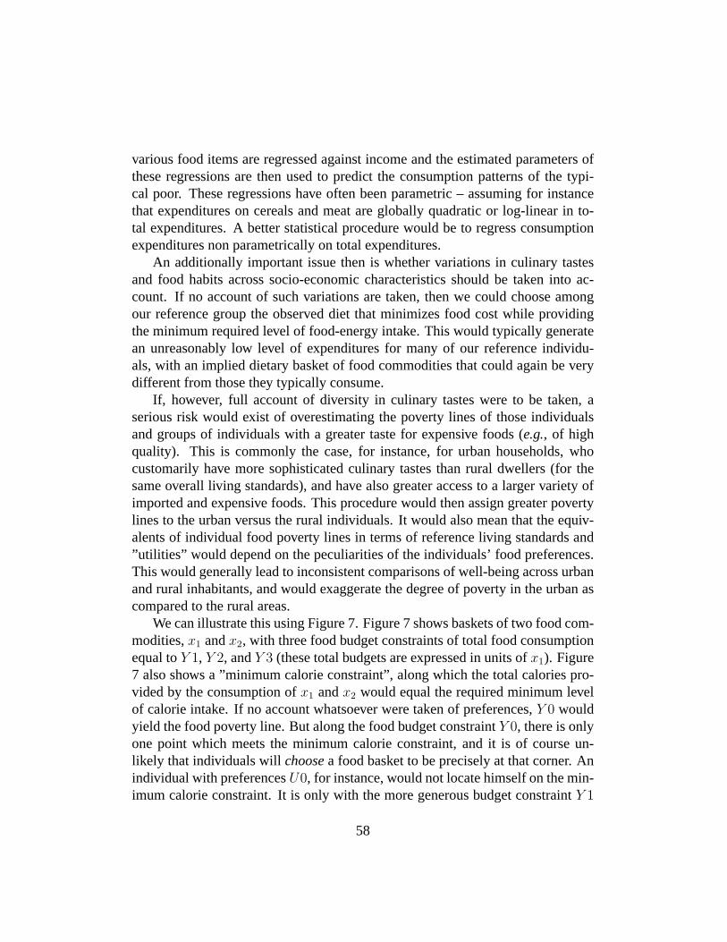
various food items are regressed against income and the estimated parameters ofthese regressions are then used to predict the consumption patterns of the typi-cal poor. These regressions have often been parametric – assuming for instancethat expenditures on cereals and meat are globally quadratic or log-linear in to-tal expenditures. A better statistical procedure would be to regress consumptionexpenditures non parametrically on total expenditures.

An additionally important issue then is whether variations in culinary tastesand food habits across socio-economic characteristics should be taken into ac-count. If no account of such variations are taken, then we could choose amongour reference group the observed diet that minimizes food cost while providingthe minimum required level of food-energy intake. This would typically generatean unreasonably low level of expenditures for many of our reference individu-als, with an implied dietary basket of food commodities that could again be verydifferent from those they typically consume.

If, however, full account of diversity in culinary tastes were to be taken, aserious risk would exist of overestimating the poverty lines of those individualsand groups of individuals with a greater taste for expensive foods (e.g., of highquality). This is commonly the case, for instance, for urban households, whocustomarily have more sophisticated culinary tastes than rural dwellers (for thesame overall living standards), and have also greater access to a larger variety ofimported and expensive foods. This procedure would then assign greater povertylines to the urban versus the rural individuals. It would also mean that the equiv-alents of individual food poverty lines in terms of reference living standards and”utilities” would depend on the peculiarities of the individuals’ food preferences.This would generally lead to inconsistent comparisons of well-being across urbanand rural inhabitants, and would exaggerate the degree of poverty in the urban ascompared to the rural areas.

We can illustrate this using Figure7. Figure7 shows baskets of two food com-modities,x1 andx2, with three food budget constraints of total food consumptionequal toY 1, Y 2, andY 3 (these total budgets are expressed in units ofx1). Figure7 also shows a ”minimum calorie constraint”, along which the total calories pro-vided by the consumption ofx1 andx2 would equal the required minimum levelof calorie intake. If no account whatsoever were taken of preferences,Y 0 wouldyield the food poverty line. But along the food budget constraintY 0, there is onlyone point which meets the minimum calorie constraint, and it is of course un-likely that individuals willchoosea food basket to be precisely at that corner. Anindividual with preferencesU0, for instance, would not locate himself on the min-imum calorie constraint. It is only with the more generous budget constraintY 1

58

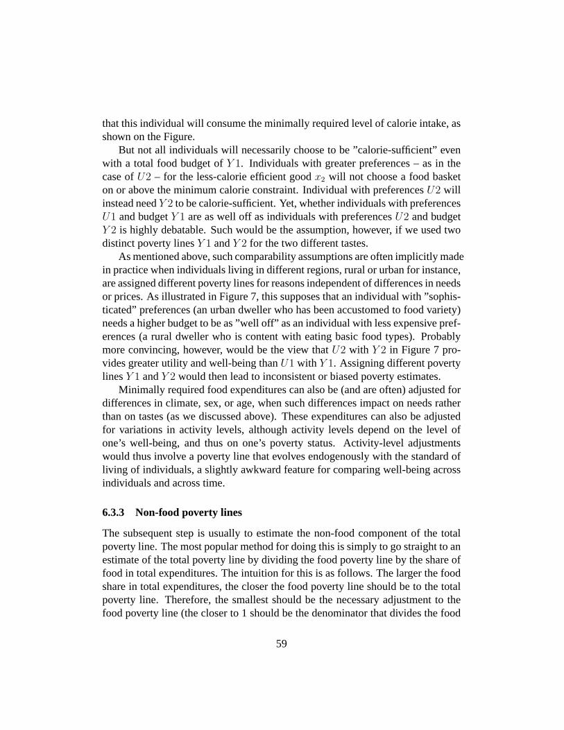
that this individual will consume the minimally required level of calorie intake, asshown on the Figure.

But not all individuals will necessarily choose to be ”calorie-sufficient” evenwith a total food budget ofY 1. Individuals with greater preferences – as in thecase ofU2 – for the less-calorie efficient goodx2 will not choose a food basketon or above the minimum calorie constraint. Individual with preferencesU2 willinstead needY 2 to be calorie-sufficient. Yet, whether individuals with preferencesU1 and budgetY 1 are as well off as individuals with preferencesU2 and budgetY 2 is highly debatable. Such would be the assumption, however, if we used twodistinct poverty linesY 1 andY 2 for the two different tastes.

As mentioned above, such comparability assumptions are often implicitly madein practice when individuals living in different regions, rural or urban for instance,are assigned different poverty lines for reasons independent of differences in needsor prices. As illustrated in Figure7, this supposes that an individual with ”sophis-ticated” preferences (an urban dweller who has been accustomed to food variety)needs a higher budget to be as ”well off” as an individual with less expensive pref-erences (a rural dweller who is content with eating basic food types). Probablymore convincing, however, would be the view thatU2 with Y 2 in Figure7 pro-vides greater utility and well-being thanU1 with Y 1. Assigning different povertylinesY 1 andY 2 would then lead to inconsistent or biased poverty estimates.

Minimally required food expenditures can also be (and are often) adjusted fordifferences in climate, sex, or age, when such differences impact on needs ratherthan on tastes (as we discussed above). These expenditures can also be adjustedfor variations in activity levels, although activity levels depend on the level ofone’s well-being, and thus on one’s poverty status. Activity-level adjustmentswould thus involve a poverty line that evolves endogenously with the standard ofliving of individuals, a slightly awkward feature for comparing well-being acrossindividuals and across time.

6.3.3 Non-food poverty lines

The subsequent step is usually to estimate the non-food component of the totalpoverty line. The most popular method for doing this is simply to go straight to anestimate of the total poverty line by dividing the food poverty line by the share offood in total expenditures. The intuition for this is as follows. The larger the foodshare in total expenditures, the closer the food poverty line should be to the totalpoverty line. Therefore, the smallest should be the necessary adjustment to thefood poverty line (the closer to 1 should be the denominator that divides the food

59

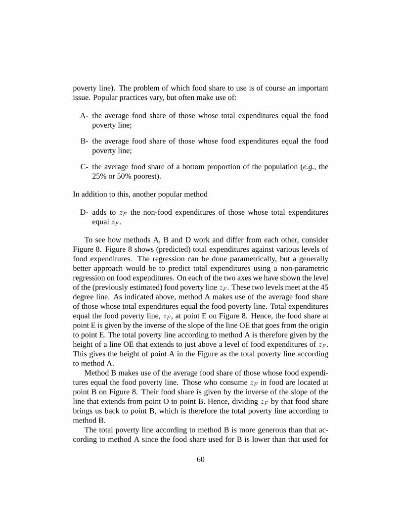
poverty line). The problem of which food share to use is of course an importantissue. Popular practices vary, but often make use of:

A- the average food share of those whose total expenditures equal the foodpoverty line;

B- the average food share of those whose food expenditures equal the foodpoverty line;

C- the average food share of a bottom proportion of the population (e.g., the25% or 50% poorest).

In addition to this, another popular method

D- adds tozF the non-food expenditures of those whose total expendituresequalzF .

To see how methods A, B and D work and differ from each other, considerFigure8. Figure8 shows (predicted) total expenditures against various levels offood expenditures. The regression can be done parametrically, but a generallybetter approach would be to predict total expenditures using a non-parametricregression on food expenditures. On each of the two axes we have shown the levelof the (previously estimated) food poverty linezF . These two levels meet at the 45degree line. As indicated above, method A makes use of the average food shareof those whose total expenditures equal the food poverty line. Total expendituresequal the food poverty line,zF , at point E on Figure8. Hence, the food share atpoint E is given by the inverse of the slope of the line OE that goes from the originto point E. The total poverty line according to method A is therefore given by theheight of a line OE that extends to just above a level of food expenditures ofzF .This gives the height of point A in the Figure as the total poverty line accordingto method A.

Method B makes use of the average food share of those whose food expendi-tures equal the food poverty line. Those who consumezF in food are located atpoint B on Figure8. Their food share is given by the inverse of the slope of theline that extends from point O to point B. Hence, dividingzF by that food sharebrings us back to point B, which is therefore the total poverty line according tomethod B.

The total poverty line according to method B is more generous than that ac-cording to method A since the food share used for B is lower than that used for

60

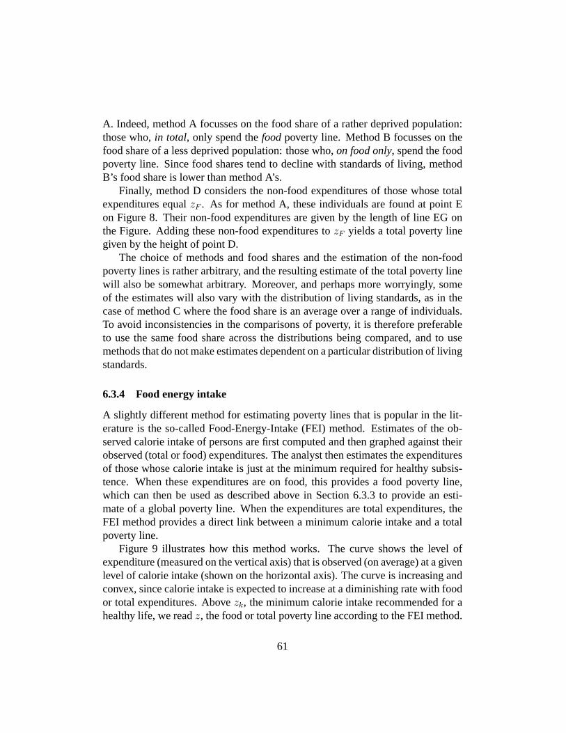
A. Indeed, method A focusses on the food share of a rather deprived population:those who,in total, only spend thefoodpoverty line. Method B focusses on thefood share of a less deprived population: those who,on food only, spend the foodpoverty line. Since food shares tend to decline with standards of living, methodB’s food share is lower than method A’s.

Finally, method D considers the non-food expenditures of those whose totalexpenditures equalzF . As for method A, these individuals are found at point Eon Figure8. Their non-food expenditures are given by the length of line EG onthe Figure. Adding these non-food expenditures tozF yields a total poverty linegiven by the height of point D.

The choice of methods and food shares and the estimation of the non-foodpoverty lines is rather arbitrary, and the resulting estimate of the total poverty linewill also be somewhat arbitrary. Moreover, and perhaps more worryingly, someof the estimates will also vary with the distribution of living standards, as in thecase of method C where the food share is an average over a range of individuals.To avoid inconsistencies in the comparisons of poverty, it is therefore preferableto use the same food share across the distributions being compared, and to usemethods that do not make estimates dependent on a particular distribution of livingstandards.

6.3.4 Food energy intake

A slightly different method for estimating poverty lines that is popular in the lit-erature is the so-called Food-Energy-Intake (FEI) method. Estimates of the ob-served calorie intake of persons are first computed and then graphed against theirobserved (total or food) expenditures. The analyst then estimates the expendituresof those whose calorie intake is just at the minimum required for healthy subsis-tence. When these expenditures are on food, this provides a food poverty line,which can then be used as described above in Section6.3.3 to provide an esti-mate of a global poverty line. When the expenditures are total expenditures, theFEI method provides a direct link between a minimum calorie intake and a totalpoverty line.

Figure 9 illustrates how this method works. The curve shows the level ofexpenditure (measured on the vertical axis) that is observed (on average) at a givenlevel of calorie intake (shown on the horizontal axis). The curve is increasing andconvex, since calorie intake is expected to increase at a diminishing rate with foodor total expenditures. Abovezk, the minimum calorie intake recommended for ahealthy life, we readz, the food or total poverty line according to the FEI method.

61

As just exposed, the FEI method may appear straightforward and simple toimplement. A number of conceptual and measurement problems are, however,hidden behind this apparent simplicity. First, the line traced on Figure9 is theex-pectedlink between expenditure and calorie intake; there is in real life a significantamount of variability around this line. How are we to interpret this variability? Ifit is due to measurement errors, then we may perhaps ignore it. If it is due to vari-ability in preferences, then we may wish to model the calorie-intake-expenditurerelationship separately for different groups of the population, as is often done inpractice, for urban and rural areas for instance. As in the cost-of-basic-needsmethod, however, we then run the risk of estimating higher poverty lines for thosegroups that have more expensive or sophisticated tastes for food. This would leadto inconsistent comparisons of well-being and poverty, as discussed in Section6.3.2.

To compute expected expenditure (given the variability of actual observedspending) at a given calorie intake, we can estimate the parameters of a para-metric regression linking expenditures to calorie intake. The regression is oftenpostulated to be log-linear or quadratic. This parametric specification supposes,however, that the functional relationship between expenditures and calorie intakeis known by the analyst, up to some unknown parameter values. This is unlikelyto be true everywhere, especially for those far from the level of calorie intake ofinterest (e.g., those at the lower and upper tails of the distribution of spending andcalorie intake). In such cases, the parametric procedure will make the estimatedexpenditure poverty line affected by the presence of ”outliers” that are relativelyfar from the minimum level of calorie intake. This procedure will then generate abiased estimator of the ”true” poverty line.

An alternative approach estimates the link between expenditures and calorieintake non parametrically. A non-parametric regression does not impose a fixedfunctional relationship between calorie intake and expenditures along the entirerange of calorie intake. On the contrary, it allows a fair amount of flexibilityby estimating the link between the two variables through a local weighting proce-dure. The local weighting procedure looks at the expenditures of those individualswith a calorie intake in the ”region” of the specified minimum calorie intake. Itweights those values with weights that decrease rapidly with the distance from theminimum calorie intake. Hence, those with calorie intakes far from the minimumspecified level will contribute little to the estimated expenditure needed to attainthat minimum level. The results using this method are thus less affected by thepresence of ”outliers” in the distribution of living standards, and less prone to bi-ases stemming from an incorrect specification of the link between spending and

62

calorie intake.

6.3.5 Illustration for Cameroon

To see whether these differences in methodologies matter, consider the case ofCameroon. Table4 shows the result of estimating food, non-food and total povertylines for the whole of Cameroon and for each of 6 regions separately. Note thatthe figures are in Francs CFA adjusted for price differences, with Yaounde beingthe reference region. The food poverty line was estimated using the FEI methodat 2400 calories per day per adult equivalent. A non parametric regression usingDAD was performed for the whole of Cameroon and separately for each of the 6regions. The lower non-food poverty line was obtained (non parametrically) usingmethod D in section6.3.3, and the upper non-food poverty line using method B.Again, the relevant regressions were carried out for the whole of Cameroon andseparately for each of the 6 regions.

As can be seen, the link between calorie intake and food expenditures variessystematically across regions. Expected food expenditure at 2400 calories per dayare significantly higher in urban areas (Yaounde, Douala and Other Cities) than inthe rural ones. In Douala, for instance, a household would need 408 Francs CFAper day per adult equivalent to reach an intake of 2400 calories per day. In theHighlands, no more than 170 Francs CFA would on average be needed. The linkbetween food and total expenditures also varies across the regions in Cameroon.Combined with the different estimates for the food poverty lines, this leads tovery significant variations across regions in the total poverty lines. Using methodD, a lower total poverty line of 589 Francs CFA is obtained for Douala, but thatsame poverty line is only 235 Francs CFA. Note also that the choice of methodB vsmethod D has a very significant impact on the estimate of the total povertyline. For the whole of Cameroon, the lower and the upper total poverty lines arerespectively 373 and 534 Francs CFA, a difference of 43%.

Unsurprisingly, these large differences across regions and across methods havea large impact on poverty estimates and on regional poverty comparisons. This isillustrated in Table6, which shows the proportion of individuals underneath var-ious poverty lines for various indicators of well-being. ”Calorie poverty” (firstcolumn) is fairly constant across Cameroon. In the whole of Cameroon, 68.1% ofthe population was observed to consume less than 2400 calories per day per adultequivalent. This proportion varies between 59.9% (for Other Cities) and 86.5%(for Forest) across regions. Roughly the same limited variability and the samepoverty rankings appear when food poverty is estimated using for each region its

63

own food poverty line (third column). However, when acommonfood poverty lineis used to assess food poverty in each region (second column), national povertystays roughly unchanged at around 69% but urban regions now appear signifi-cantly less poor than the rural ones. For instance, the poverty headcount in Douala(42.0 %) is now only half that of the Highlands (82.5 %).

The rest of Table6confirms these lessons. When a common poverty line isused to compare the regions, rural areas are very significantly poorer than urbanones. When region-specific poverty lines are used, these differences are muchreduced, and the regional rankings are often even reversed. For example, usinga common lower total poverty line (fourth column), the Highlands have a head-count ratio more than three times that of the urban regions. When regional lowertotal poverty lines are used instead, the Highlands become prominently the leastpoor of all regions. Setting common as opposed to regional poverty lines canthus have a crucial impact on poverty rankings and the determination of subse-quent poverty alleviation policies. The choice of a lower as against an upper totalpoverty line also makes a difference. For the whole of Cameroon, the proportionof the Cameroonian population in poverty increases from 43.9% to 68.0% whenwe move from a common lower total poverty line (fourth column) to a commonupper total poverty line (sixth column). Clearly, this changes significantly one’sunderstanding of the incidence of poverty in Cameroon.

These results also implicitly caution that the choice of well-being indicatorsis not neutral to the identification of the poor. In our context, this is because thecorrelation between calorie intake, food expenditure and total expenditure is im-perfect. Table?? indicates, for example, that in bidimensional poverty analysesusing any two of these three indicators of well-being, around 20% to 25% of thepopulation is characterized as poor in one dimension but non poor in the other. Inthe first part of??, we note for instance that 11.2% of the population would bejudged poor in terms of calorie intake but not poor in terms of food expenditure.Conversely, 9.6% of the population would be deemed non poor in terms of calo-rie intake but poor in terms of food expenditure. These proportions are slightlyhigher for the other bidimensional poverty analyses, which compare food withtotal expenditure poverty, and calorie with total expenditure poverty, respectively.

6.3.6 Relative and subjective poverty lines

Relative poverty linesThere are two other popular methodologies for the estimation of poverty lines.

The first deals with relative poverty lines, which, as we saw above, can be useful

64

to determine the commodities needed for ”living without shame” and for partici-pating in the ”prevailing consumption level”. A relative poverty line is typicallyset as an arbitrary proportion (often around 50%) of the mean or the median ofliving standards. Clearly, such a poverty line will vary with the central tendencyof the distribution of living standards, and will not be the same across regions andtime. One awkward feature of the use of a relative poverty line approach is that apolicy which raises the living standards of all, but proportionately more those ofthe rich, will increase poverty, although the absolute living standards of the poorhave risen. Conversely, a natural catastrophe which hurts absolutely everyone willdecrease poverty if the rich are proportionately the most hurt. When used alone,relative poverty lines can thus be shown to drift the analysis towards the conceptof relative inequality, and away from absoluteness of deprivation in any of thepoverty measurement spaces define above. Because of this, they are probably bestused in conjunction with absolute living standard thresholds, at least when theaim is to capture both absolute deprivation in basic physiological capabilities andsocial exclusion and relative deprivation in more social capabilities.

Subjective poverty linesThe second alternative poverty line approach relies on the use of subjective

information on the link between living standards and well-being. One source ofinformation comes from interviews on what is perceived to be a sound povertyline, using a query found for instance in Goedhartet al. (1977):

We would like to know which net family income would, in your cir-cumstances, be the absolute minimum for you. That is to say, that youwould not be able to make both ends meet if you earned less.

The answers are subsequently regressed on the living standards of the respondents.The subjective poverty line is given by the point at which the predicted answer tothe minimum income question equals the living standard of the respondents. Theidea is that unless someone earns that poverty line, he will not truly know that itis indeed the appropriate minimum income needed to ”make both ends meet”.

This method is illustrated on Figure10. Each point represents a separate an-swer to the above query, namely, the minimum income judged to be needed tomake both ends meet as a function of the actual income of the respondents. Thefilled line shows the predicted response of individuals at a given level of income.For low income levels, this predicted minimum subjective income is well abovethe respondents’ income. The predicted minimum subjective income increaseswith actual income, but not as fast as income itself, such that atz∗ (on the 45-degree line), the predicted minimum subjective income equals actual income.

65

One difficulty with the subjective approach is the sensitivity of poverty lineestimates to the formulation of interview questions. Perhaps a more fundamentaldisquieting output is the considerable variability in the answers provided, evenwithin groups of relatively socio-economically homogeneous respondents. Thepresence of this variability is apparent on Figure10 with points sometimes quitefar away from the predicted response line. This variability has some awkward con-sequences. On Figure10, for instance, pointa is a point at which someone wouldbe judged poor according to the subjective income method, since his income fallsbelow z∗. An individual ata feels, however, that his income exceeds the mini-mum income he feels to be needed (pointa is to the right of the 45-degree line).He would therefore feel that he is not poor. Conversely, someone at pointb feelsthat he is poor, since his reported minimum income exceeds his actual income,but he would be judged not to be poor by the subjective poverty line method.

How, therefore, ought we to interpret this variability? Is it due to measurementerrors? If so, then we may best ignore it. Is it rather that the link between livingstandards and real well-being varies systematically within homogeneous groupsof people? If so, then we should not attempt to use living standards or other director indirect indicators of well-being to classify the poor and the non poor. Instead,we should perhaps take individuals at word on whether they declare themselves tobe poor or not. But this would alternatively raise important practical problems forthe assessment and the implementation of public policy. Can public policy relyappropriately and confidently for its implementation on the provision of subjectiveinformation on the part of individuals?

Subjective poverty lines with discrete informationAn alternative approach to estimating subjective poverty lines is to ask re-

spondents whether they feel that their living standards are below the poverty line,without direct indications of what the value of that poverty line may well be. An-swers are coded 0 or 1 – according to whether respondents feel that they are pooror not – alongside the respondents’ living standards. This is illustrated in Figure11. Each ”dot” is an observation of whether a respondent of a certain income levelfelt poor (1) or not (0). The implicit assumption is that respondents compare theirincome to acommonsubjective poverty linez∗. z∗ is unobserved and must be es-timated. Not everyone with an income belowz∗ says that he is poor; conversely,not everyone abovez∗ says that he is not poor. These ”classification errors” wouldbe explained by measurement and/or misreporting errors. Hence, on Figure11,there are ”false poor” and ”false rich”, as shown within the ellipses at the bottomleft and at the top right of the Figure.

The estimation ofz∗ proceeds by minimizing the probability of observing false

66

poor and false rich. Said differently, the estimator ofz∗ is that which minimizesthe likelihood of observing observations within the ellipses in Figure11.

67

7 The measurement of progressivity, equity and re-distribution

7.1 Taxes and concentration curves

Let X andN represent respectively gross and net incomes. Gross income is pre-tax and/or pre-transfer income, and net income is post-tax and/or post-transferincome. The mapping of gross incomes into net incomes is done byT , with N =X − T . For expositional simplicity, we assume throughout that gross incomesare exogeneous. We can expect a part ofT to be a tax and transfer function,T (X), that depends on the value of gross incomeX. For several reasons, wealso expectT to be stochastically related toX. In real life, taxes and transfersdepend on a number of variables other than gross incomes, such as family sizeand composition, age, sex, area of residence, sources of income, consumption andsavings behaviour, and the ability to avoid taxes or claim transfers. Thus, we canthink of T as being a stochastic function ofX,

T = T (X) + ν, (71)

whereν is a stochastic tax determinant. We will denote byFX,N(·, ·) the jointcumulative distribution function (cdf) of gross and net income. LetX(p) be thep-quantile function for gross incomes, andN(q) the q-quantile function for netincomes. LetFN |X=x(·) be thecdf of N conditional onX = x. Theq-quantilefunction for net incomes conditional on ap-quantile value for gross incomes isthen technically defined asN(q|p) = infs > 0|FN |X=X(p)(s) ≥ q for q ∈ [0, 1].N(q|p) thus gives the net income of the individual whose net income rank isqamong all those whose rank isp in the distribution of gross incomes.

The expected net income of those at rankp in the distribution of gross incomeis given by:

N(p) =∫ 1

0N(q|p)dq. (72)

The expected net tax of those at rankp in the distribution of gross income is thengiven by:

T (p) = N(p)−X(p). (73)

The concentration curve forT is:

68

CT (p) =

∫ p0 T (q)dq

µT

(74)

whereµT =∫ 10 T (p)dp = µN − µX is average taxes across the population.CT (p)

shows the proportion of total taxes paid by thep bottom proportion of the popu-lation. In practice, concentration curves are often estimated by ordering a finitenumber of sample observations(X1, T1), ..., (Xn, Tn) in increasing values of grossincomes, such thatX1 ≤ X2 ≤ ... ≤ Xn, with percentilespi = i/n, i = 1, ..., n.For i = 1, ...n, the discrete (or “empirical”) concentration curve for taxes is thendefined as:

CT (p = i/n) =1

nµT

i∑

j=1

Tj. (75)

As for the empirical Lorenz curves, other values ofCT (p) can be estimated byinterpolation. The concentration curveCN(p) for net incomes is analogously de-fined as:

CN(p) =

∫ p0 N(q)dq

µN

(76)

and typically estimated as:

CN(p = i/n) =1

nµN

i∑

j=1

Nj (77)

where theNj have been ordered in increasing values of the associatedXj. NotethatCN(p) is different from the Lorenz curve of net incomes,LN(p), defined as:

LN(p) =

∫ p0 N(q)dq

µN

. (78)

Empirically, the Lorenz curve for net income is typically estimated as

LN(p = i/n) =1

nµN

i∑

j=1

Nj (79)

69

where the observations have been ordered in increasing values ofnet incomes.Thus,CN(p) sums up the expected value of net incomes (conditional on a per-centile of gross incomes) up to gross income percentilep. LN(p), however, sumsup net incomes up to a net income percentilep. We can show thatCN(p) will neverbe lower thanLN(p), and will be strictly greater thanLN(p) for at least one valueof p if there is “reranking” in the redistribution of incomes (this feature will proveuseful later in building indices of reranking)3. Intuitively, CN(p) cumulates somenet incomes whose percentiles in the net income distribution exceedp. These arenet incomes that are high compared to the expected net income at a gross incomeof percentilep or lower. Such high incomes are nevertheless possible, however,due to the stochastic termν. LN(p) only cumulates the net incomes whose per-centile in the net income distribution isp or lower. Hence,CN(p) ≥ LN(p). Thiscan also be seen by comparing the estimators in equations (77) and (79). In (79),observations ofNj are cumulated in increasing values ofNj, but in (77), obser-vations ofNj are cumulated in increasing values ofXj, which means that somehigher values ofNj may be cumulated before some lower ones.

Denote the average tax rate as a proportion of average gross income ast, witht = µT /µX . Whent 6= 0, we can show the following:

CN(p) − LX(p) =t

1− t[LX(p) − CT (p)] . (80)

For a positivet, this indicates that the more concentrated are the taxes among thepoor (the smaller the differenceLX(p)−CT (p)), the less concentrated among thepoor will net incomes be. The reverse is true for transfers (negativet): the moreconcentrated they are among the poor, the more concentrated net income is amongthe poor. This link will prove useful later in defining indices of tax progressivity.

7.2 Indices of concentration

As for the Lorenz curves and the S-Gini indices of inequality, we can aggregatethe distance betweenp and the concentration curvesC(p) to obtain indices ofconcentration. These indices of concentration are useful to compute aggregateindices of progressivity and vertical equity. More generally, they can also serveto decompose the inequality in total income or total consumption into a sum ofthe inequality in the components of that total income or consumption, such as dif-ferent sources of income (different types of earnings, interests, dividends, capital

3In a continuous distribution, a sufficient condition for reranking is thatν is not degenerate,namely, that it is not a constant.

70

gains, taxes, transfers, etc.) or different types of consumption (of food, clothing,housing, etc.). To define indices of concentration, we can simply weight the dis-tancep−C(p) by a weightκ(p), of which a popular form is again given byκ(p; ρ)in equation (12). This gives the following class of S-Gini indices of concentration:

IC(ρ) =∫ 1

0(p− C(p))κ(p; ρ)dp. (81)

For instance, letX1 andX2 be two types of consumption, and letX = X1+X2

be total consumption. LetCX1(p) and CX2(p) be the concentration curves ofeach of the two types of consumption (usingX as the ordering variable). Theconcentration indices forX1 andX2 are as follows :

ICX1(ρ) =∫ 1

0(p− CX1(p))κ(p; ρ)dp (82)

and

ICX2(ρ) =∫ 1

0(p− CX2(p))κ(p; ρ)dp. (83)

Inequality inX can then be decomposed as a sum of the inequality inX1 and inX2. The Lorenz curve for total consumption is given by:

LX(p) =(µX1CX1(p) + µX2CX2(p))

µX

(84)

which is a simple weighted sum of the concentration curves for each of the twotypes of consumption. The index of inequality in total consumption is similarlya simple weighted sum of the concentration indices of each of the two types ofconsumption:

IX(ρ) =µX1ICX1(ρ) + µX2ICX2(ρ)

µX

. (85)

For givenµX1 andµX2, the higher the concentration indicesICX1(ρ) andICX2(ρ),the larger the S-Gini index of inequality in total consumption. The higher the shareµXi

/µX of the more highly concentrated expenditure, the higher the inequality intotal expenditures.

71

7.3 Progressivity comparisons

7.3.1 Deterministic tax and benefit systems

Let us for a moment assume that the tax system is non-stochastic (or determinis-tic), namely, thatν equals a constant zero. Suppose also for now that the deter-ministic tax system does not rerank individuals, or equivalently thatT (1)(X) ≤ 1.Denote the average rate of taxation at gross incomeX by t(X) = T (X)/X. Anet tax (possibly including a transfer or subsidy)T (X) is said to be progressive ifthe average rate of taxation increases withX, that is, ift(1)(X) > 0; it is propor-tional if t(1)(X) = 0, and it is regressive ift(1)(X) < 0. There are two popularmeasures to capture the change in taxes and net income as gross income increases.One is the elasticity of taxes with respect toX, and is called Liability Progression,LP (X):

LP (X) =X

T (X)T (1)(X) =

T (1)(X)

t(X)(86)

and is therefore simply the ratio of the marginal tax rate over the average taxrate. The larger this measure at everyX, the more concentrated among the richerare the taxes. It is possible to show that a tax system is uniformly progressive(namely,t(1)(X) > 0 everywhere) ifLP (X) > 1 everywhere. One problem withLP (X) is that it is not defined whenT (X) = 0, and that it is awkward to interpretwhen a net tax is sometimes negative and sometimes positive across gross income.Another problem is that it is linked to the relative distribution of taxes, not with therelative distribution of the associated net incomes. These problems are avoided bya second measure, called Residual Progression (RP (X)), which is the elasticityof net income with respect to gross income:

RP (X) =∂(X − T (X))

∂X· X

N=

1− T (1)(X)

1− t(X). (87)

Unlike LP (X), RP (X) is well defined and easily interpretable even when taxesare sometimes negative, positive or zero, so long as gross and net incomes arestrictly positive.

It is then possible to show that a tax system is uniformly progressive (again,this means thatt(1)(X) > 0 everywhere) ifRP (X) < 1 everywhere. This willmake the distribution of net incomes unambiguously more equal than the distri-bution of gross incomes, regardless of that actual distribution of gross incomes.Moreover, if the residual progression for a tax systemA is always lower than thatof a tax systemB, whatever the value ofX, then the tax systemA is said to be

72

uniformly more progressive than the tax systemB, and the distribution of net in-comes will always be more equal underA than underB, again regardless of thedistribution of gross incomes.

Hence, an important distributive consequence of progressive taxation is tomake the inequality of net incomes lower than that of gross income. Analo-gously, proportional taxation will not change inequality, and regressive taxationwill increase inequality. The more progressive the tax system, the more inequality-reducing it is. To check whether a deterministic tax system is progressive, pro-portional or regressive, we may thus simply plot the average tax rate as a functionof X and observe its slope. Alternatively, we may estimate and graph its liabilityprogression or its residual progression at various values ofX. To check whethera tax system is more progressive (and thus more redistributive) than another one,we simply plot and compare the elasticity of net incomes with respect to grossincomes. All of this can be done using non-parametric regressions ofT (X) andN againstX.

Another informative descriptive approach is to compare the share in taxes andbenefits to the share in the population of individuals at various ranks in the dis-tribution of income. This is most easily done by plotting on a graph the ratiosT (X)/µT or T (p)/µT for various values of gross incomeX or ranksp in thepopulation. If these ratios exceed 1, then those individuals with those incomesor ranks pay a greater share of total taxes than their population share. A similarintuition applies whenT (·) is a benefit: a ratioT (X)/µT or T (p)/µT that exceeds1 indicates that the benefit share exceeds the population share.

A competing descriptive tool is to plot the ratio of taxes or benefitsT (X)over gross incomeX, that is,T (X)/X, perhaps assessed at some rankp to giveT (p)/X(p). Such a graph shows how the average tax rate evolves with grossincome or ranks. This can show quite a different picture from that shown byT (X)/µT or T (p)/µT .

7.3.2 General tax and benefit systems

Although graphically informative, the above simple descriptive approaches present,however, some problems. First, ifT (1)(X) > 1, the tax system will induce rerank-ing, even if it is a deterministic function ofX. As we will see below, reranking(and, more generally, horizontal inequity) decreases the redistributive effect oftaxation, besides being of course of significant ethical concern in its own right.Second, and more importantly in empirical applications, taxes are typically not adeterministic function of gross income, and randomness in taxes will introduce

73

greater variability and inequality in net incomes than the above deterministic ap-proach would predict.X − T (X) may then be an unreliable guide to the distri-bution of net incomes. Randomness in taxes will also introduce further reranking.These two features will reduce the redistributive effect of the tax, and may even inthe most extreme cases increase inequality even when the “deterministic trend” ofthe tax is progressive, or such thatt(1)(X) > 0. Finally, the actual redistributioneffected by taxes depends on the distribution of gross incomes, and not only onthe shape of the tax functionT . Said differently, the actual redistributive effectof liability or residual progression will depend on the actual distribution of grossincomes.

To deal with these difficulties, we can use the actual distribution of taxesT andnet incomesN (instead of their predicted valuesT (X) andX − T (X)) to deter-mine whether the actual tax system is progressive and inequality-reducing. Thereare two leading approaches for this exercise. The first is the Tax-Redistribution(TR) approach, and the second is the Income-Redistribution (IR) approach.

A tax T is beTR-progressive if

CT (p) < LX(p) for all p ∈]0, 1[. (88)

A benefitB is TR-progressive if

CB(p) > LX(p) for all p ∈]0, 1[. (89)

A tax T ′ is moreTR-progressive than a taxT 0 if

CT ′(p) < CT 0(p) for all p ∈]0, 1[. (90)

A benefitB′ is moreTR-progressive than a benefitB0 if

CB′(p) > CB0(p) for all p ∈]0, 1[. (91)

A tax T is moreTR-progressive than a benefitB if

LX(p) − CT (p) > CB(p) − LX(p) for all p ∈]0, 1[. (92)

A tax (and/or a transfer)T is IR-progressive if

CN(p) > LX(p) for all p ∈]0, 1[. (93)

A tax (and/ or a transfer)T ′ is moreIR-progressive than a tax (and/or a trans-fer) T 0 if

CN ′(p) > CN0(p) for all p ∈]0, 1[. (94)

74

These twoTR andIR approaches are consistent with the use above of lia-bility and residual progression in a deterministic tax system. Ift(1)(X) > 0 andT (1)(X) ≤ 1 (namely, no reranking), then, whatever the actual distribution ofgross incomes,T (X) is bothTR- andIR-progressive.

Note that these progressivity comparisons have as a reference point the initialLorenz curve. In other words, a tax is progressive if the poorest individuals beara share of the total tax burden that is less than their share in total gross income.As mentioned above, another view is that the poor should pay a tax burden thatis proportional to their share in the population. This is more often argued in thecontext of benefits – the reference point to assess the equity of public expendituresis population share. The analytical framework above can easily allow for thisalternative view – simply by replacingLX(p) by p in the above definitions ofTRprogressivity. This will make more stringent the conditions to declare a benefitprogressive, but it will also make it easier for a tax to be declared progressive –see (88) and (89).

7.4 Reranking and horizontal inequity

As is well-known, the assessment of tax and transfer systems draws on two fun-damental principles: efficiency and equity4 . The former relates to the presenceof distortions in the economic behavior of agents, while the latter focuses on dis-tributive justice. Vertical equity as a principle of distributive justice is rarely ques-tioned as such, although the extent to which it must be precisely weighted againstefficiency is of course a matter of intense disagreement among policy analysts. Inthis section, we examine in more detail a more neglected aspect of the notion ofequity: horizontal equity (HE) in taxation (including negative taxation).

Two main approaches to the measurement ofHE are found in the literature,which has evolved substantially in the last twenty years. The classical formulationof theHE principle prescribes the equal treatment of individuals who share thesame level of welfare before government intervention.HE may also be viewedas implying the absence of reranking: for a tax to be horizontally equitable, theranking of individuals on the basis of pre-tax welfare should not be altered by afiscal system.

Why should concerns for horizontal equity influence the design of an opti-mal tax and transfer system? Several answers have been provided, using either of

4This section draws heavily from a joint paper written with Vincent Jalbert and AbdelkrimAraar.

75

two approaches. The traditional or “classical” approach definesHE as the equaltreatment of equals (see Musgrave (1959)). While this principle is generally wellaccepted, different rationales are advanced to support it. First, a tax which dis-criminates between comparable individuals is liable to create resentment and asense of insecurity, possibly also leading to social unrest. This is supported by thesocio-psychological literature which shows that exclusion and discrimination havean impact both on individual well-being and on social cohesion and welfare. Forinstance, status/role structure theory indicates that one’s relative socio-economicposition (and its variability) “may give rise to definable and measurable socialand psychological reactions, such as different types of alienation” (Durant andChristian (1990), p.210).

Second, the principles of progressivity and income redistribution, which arekey elements of most tax and transfer systems, are generally undermined byHI(as we shall see in our own treatment below). This has indeed been one of themain themes in the development of the reranking approach in the last decades (seefor instance Atkinson (1979) and Jenkins (1988)). Hence, a desire forHE maysimply derive from a general aversion to inequality, without any further appeal toother normative criteria. Feldstein (1976) also notes that when utility functionsare identical across individuals, a utilitarian social welfare function is maximizedwhen equal incomes are taxed equally. This result then makes the principle ofHE become a corollary of the principle of VE. A separate justification ofHEwould, however, generally be required when preferences are heterogeneous (theyusually are), and because in some circumstances a random tax can otherwise befound to be optimal (Stiglitz (1982)).HI may moreover suggest the presence ofimperfections in the operation of the tax and transfer system, such as an imperfectdelivery of social welfare benefits, attributable to poor targeting or to incompletetake-up (see Duclos (1995b)). It can also signal tax evasion, which caninter aliacost the government significant losses of tax revenue (see Bishopet al. (1994)).

Third,HE can be argued to be an ethically more robust principle than VE (VErelates to the reduction of welfare gaps between unequal individuals). TheHEprinciple is often seen as a consequence of the fundamental moral principle of theequal worth of human beings, and as a corollary of the equal sacrifice theoriesof taxation. Depending on the retained specification of distributive fairness, therequirements of vertical justice can vary considerably, while the principle of hor-izontal equity remains essentially invariant (Musgrave (1990)). Plotnick (1982)also supports this view by arguing thatHI in the redistributive process wouldcause a loss of social welfare relative to an horizontally equitable tax, regardlessof any VE value judgments on the final distribution. This has led several authors

76

(including Stiglitz (1982), Balcer and Sadka (1986) and Hettich (1983)) to advo-cate thatHE be treated as a separate principle from VE, and thus to form one ofthe objectives between which an optimal trade-off must be sought in the setting oftax policy.

The value of studying classicalHI has nonetheless been questioned by a fewauthors, among whom figures Kaplow (1989, 1995), who rejects the premise thatthe initial distribution is necessarily just (see also Atkinson (1979) and Lermanand Yitzhaki (1995)) and adds that utilitarianism and the Pareto principle mayjustify the unequal treatment of equals (as seen above)5. A number of authorshave also expressed dissatisfaction with the classical approach toHE becauseof the implementation difficulties it was seen to present. Indeed, since no twoindividuals are ever exactly alike in a finite sample, it was argued (seeinter aliaFeldstein (1976) and Plotnick (1982,1985)) that analysis of equals had to proceedon the basis of groupings of unequals which were ultimately arbitrary and whichrepresented “an artificial way to salvage empirical applicability” (Plotnick (1985),p. 241). The proposed alternative was then to linkHI and reranking and to notethat the absence of rerankingimplies the classical requirement ofHE: “the taxsystem should preserve the utility order, implying that if two individuals wouldhave the same utility level in the absence of taxation, they should also have thesame utility level if there is a tax” (Feldstein (1976), p.94)6.

Various other ethical justifications have also been suggested for the require-ment of no-reranking. For normative consistency, King (1983) argues for addingthe qualification “and treating unequals accordingly” to the classical definition ofHE, by which it then becomes clear that classicalHE also impliesthe absenceof reranking. Indeed, if two unequals are reranked by some redistribution, thenit could be argued at a conceptal level that at a particular point in that processof redistribution, these two unequals became equals and were then made unequal(and reranked), thus violating classicalHE. Hence, from the above, “a neces-sary and sufficient condition for the existence of horizontal inequity is a changein ranking between the ex ante and the ex post distributions” (King (1983), p.102). King (1983) then proposes an additively separable social welfare functionthat is characterized by a parameter of aversion to horizontal inequity and ver-

5The same is true for the reranking of individuals, which is discussed below. See alsoKing(1983), who sees this implication as a flaw of strict utilitarianism since it ignores the fair-ness of the redistributive process.

6The requirement of no reranking further implies that marginal tax rates should not exceed100%, which can be taken as a basic economic requirement for incentive preservation and effi-ciency. On this, seeinter alia Lambert and Yitzhaki (1995).

77

tical inequality. This function decreases with the distance of each net incomefrom its order-preserving level of net income. Chakravarty (1985) also argues thatreranking causes an individual’s utility to differ from what it would have beenotherwise, and moreover suggests that this difference reduces the final level of in-dividual utility, creating a loss of social welfare as measured again by a utilitarianwelfare function.

The theory of relative deprivation also suggests that people often specificallycompare their relative individual fortune with that of others in similar or closecircumstances. The first to formalize the theory of relative deprivation, Davis(1959), expressly allowed for this by suggesting how comparisons with similarvsdissimilar others lead to different kinds of emotional reactions; he used the expres-sion “relative deprivation” for “in-group” comparisons (i.e., for HI), and “relativesubordination” for “out-group” comparisons (i.e., for VE) (Davis (1959), p.283).Moreover, in the words of Runciman (1966), another important contributor to thattheory, “people often choose reference groups closer to their actual circumstancesthan those which might be forced on them if their opportunities were better thanthey are” (p.29).

In a discussion of the post-war British welfare state, Runciman also notes that“the reference groups of the recipients of welfare were virtually bound to remainwithin the broadly delimited area of potential fellow-beneficiaries. It was anoma-lies within this area which were the focus of successive grievances, not the relativeprosperity of people not obviously comparable” (p.71). Finally, in his theory ofsocial comparison processes, Festinger (1954) also argues that “given a range ofpossible persons for comparison, someone close to one’s own ability or opinionwill be chosen for comparison” (p.121). In an income redistribution context, itis thus plausible to assume that comparative reference groups are established onthe basis of similar gross incomes and proximate pre-tax ranks, and that individ-uals subsequently make comparisons of post-tax outcomes across these groups.Individuals would then assess their relative redistributive ill-fortune in referencegroups of comparables by monitoringinter alia whether they are overtaken by orovertake these comparables in income status, thus providing a plausible “micro-foundation” for the use of no-reranking as a normative criterion.

This suggests that comparisons with close individuals (but not necessarily ex-act equals) would be at least as important in terms of social and psychologicalreactions as comparisons with dissimilar individuals, and thus that analysis ofHIand reranking in that context should be at least as important as considerations ofVE. It also says that, although classicalHI and reranking are both necessary andsufficient signs ofHI, they are (and will be perceived as) different manifestations

78

of violations of theHE principle7. Hence, it seems reasonable that VE and theno-reranking requirement be assessed separately from the classical requirementof equal treatment of equals when assessing the impact of taxes and transfers onsocial welfare8.

How do we analyze this empirically?Show the variability ofT (X): σT (X) andσT (X(p)Also: a tax (and/or a transfer)T causes reranking (and hence horizontal in-

equity) if CN(p) > LN(p) for at least one value ofp ∈]0, 1[.

7.5 Redistribution

It is possible to decompose the net redistributive effect of taxes and transfers intocomponents that are called vertical equity (V E) and horizontal inequity (HI).TheV E effect measure the tendency of a tax system to “compress” the distribu-tion of net incomes. As we will see, it is linked to the progressivity of the taxsystem. TheHI term, which contributes negatively to the net redistributive ef-fect of the tax system (hence the use of horizontal “inequity”), accounts for the“unequal tax treatment of equals”. Depending on the choice of the underlyingsocial welfare function or inequality index, the horizontal inequity term can eithertake the form of a “classical” horizontal inequity effect or of a “reranking” effect.Our use of Lorenz and concentration curves and of the associated S-Gini indicesof inequality and redistribution will make us focus here on reranking indices ofhorizontal inequity.

The difference between the Lorenz curve of net and gross incomes is given by:

LN(p)− LX(p) = CN(p)− LX(p)︸ ︷︷ ︸V E

− (CN(p)− LN(p))︸ ︷︷ ︸HI

. (95)

The first term,V E, is clearly linked to the definition ofIR-progressivity in equa-tion (93). As shown in equation (80), it can also be expressed in terms ofTR-progressivity whent 6= 0:

7This is nicely discussed in the survey by Jenkins and Lambert (1999) and by Plotnick’s (1999)comments on it. See also Kaplow (1989), who observes that the goal of limiting reranking mayconflict with that of limiting the unequal treatment of equals.

8In the words of Feldstein (1976): “The problem for tax design is therefore to balance thedesire for horizontal equity against the utilitarian principle of welfare maximisation. Balancingthese two goals requires an explicit measure of the departure from horizontal equity.” (p.83).

79

CN(p)− LX(p) =t

1− t[LX(p)− CT (p)] . (96)

Furthermore, if there is more than one tax and/or benefit that make upT , wecan decompose totalV E as a sum of theIR andTR progressivity of each tax andtransfer. Lettj be the overall average rate of the taxTj, with j = 1, ..., J , suchthat

∑Jj=1 tj = t, and letCTj

(p) andCNj(p) be the concentration curves of net

income and taxes corresponding to taxTj. Then:

CN(p)− LX(p) =J∑

j=1

(1− tj)

(1− t)(CNj

(p)− LX(p)) (97)

whereCNj(p)−LX(p) is the vertical equity of tax or transferj at percentilep, and

again can be easily seen to be an element of the definition ofIR-progressivity.Each of theseV E contributions can also be expressed as a a function ofTRprogressivity atp (whentj = 0):

CNj(p)− LX(p) =

tj1− tj

[LX(p)− CTj

(p)]. (98)

7.6 Indices of progressivity and redistribution

As for comparisons of inequality and concentration, it is often useful to summarisethe progressivity, vertical equity, horizontal inequity as well as the redistributiveeffect of taxes and transfers into summary indices. We can do this by weighting thedifferences expressed above by the weights of the S-Gini indices(κ(p; ρ)) to ob-tain S-indices ofTR-progressivity (IT (ρ)), IR-progressivity and vertical equity(IV (ρ)), horizontal inequity and reranking (IH(ρ)), and redistribution (IR(ρ)):

IT (ρ) =∫ 1

0(LX(p)− CT (p))κ(p; ρ)dp (99)

IV (ρ) =∫ 1

0(CN(p)− LX(p))κ(p; ρ)dp (100)

IH(ρ) =∫ 1

0(CN(p)− LN(p))κ(p; ρ)dp (101)

IR(ρ) =∫ 1

0(LN(p)− LX(p))κ(p; ρ)dp. (102)

These indices can also be computed as differences between S-Gini indices of in-equality and concentration:

80

IT (ρ) = ICT (ρ)− IX(ρ) (103)

IV (ρ) = IX(ρ)− ICN(ρ) (104)

IH(ρ) = IN(ρ)− ICN(ρ) (105)

IR(ρ) = IX(ρ)− IN(ρ). (106)

Many of these indices have first been proposed withρ = 2, which correspondsto the case of the standard Gini index.IT (ρ = 2) is known as the Kakwani indexof TR progressivity,IV (ρ = 2) is known as the Reynolds-Smolensky index ofIR progressivity and vertical equity, andIH(ρ = 2) is known as the Atkinson-Plotnick index of reranking. The general S-Gini formulations have been proposedby Kakwani and Pfahler (TR andIR progressivity) and Duclos (reranking).

81

8 Issues in the empirical measurement of well-beingand poverty

Poverty assessment is customarily carried out using data on households and in-dividuals. These data can be administrative (i.e., stored in government files andrecords), they can come from censuses of the entire population, or (most com-monly) they can be generated by probabilistic surveys on the characteristics andliving conditions of a population of households.

8.1 Survey issues

There are several aspects of the surveying process that are important for povertyassessment. First, there is the coverage of the survey: does it contain represen-tative information on the entire population of interest, or just on some socio-economic subgroups? Whether the representativeness of the data is appropriatedepends on the focus of the poverty assessment. A survey containing observa-tions drawn exclusively from the cities of a particular country may be perfectlyfine if the aim is to design poverty alleviation schemes within these cities; its rep-resentativeness will, however, be clearly insufficient if the objective is to assessthe allocation of resources between the country’s urban and rural areas.

Then, there is the sample frame of the survey. Surveys are usually multi-staged, and built upon strata and clusters. Stratification ensures that a certainminimum amount of information is obtained from each of a given number of ar-eas within a population of interest. Population strata are often geographic andcan represent, for instance, the different regions or provinces of a country. Clus-tering facilitates the interviewing process by concentrating sample observationswithin particular population subgroups or geographic locations. Strata are thusoften divided into a number of different levels of clusters, representing, say, cities,villages, neighborhoods, or households. A complete listing of the clusters in eachstrata is used to select randomly within each strata a given number of clusters.The selected clusters can then be subjected to further stratification or clustering,and the process continues until the last sampling units (usually households or in-dividuals) have been selected and interviewed.

Fundamental in the use of survey data is the role of the randomness of theinformation that is generated. Because households and individuals are not all sys-tematically interviewed (unlike in the case of censuses), the information generatedfrom survey data will depend on the particular selection of households and indi-

82

viduals made from a population. A poverty assessment of a given population willthen vary across the various samples that can be selected from this same popula-tion. For that reason, poverty assessments carried out using survey data will besubject to so-called ”sampling errors”, that is, to sampling variability. When gen-erating poverty assessments from sample survey data, it is therefore important torecognise and assess the statistical imprecision of the sampling results obtained.

By ensuring that a minimum amount of information (typically, a certain num-ber of observations) is obtained from each of a number of strata, stratificationdecreases the extent of sampling errors. A similar effect is obtained by increas-ing the total size of the sample: the greater the number of households surveyed,the greater on average is the precision of the estimates obtained. Conversely, bybundling observations around common geographic or socio-economic indicators,clustering tends to reduce the informative content of the observations made andthus to increase the size of the sampling errors (for a given number of observa-tions). The sampling structure of a survey also impacts on its ability to provideaccurate information on certain population subgroups. For instance, if the clusterswithin a strata represent regions, and between-region variability is large, it wouldnot be reasonable to try to use the information generated by the selected regionsto depict poverty in the other, non-selected, regions.

Survey data are also fraught with measurement and other ”non-sampling” er-rors. For instance, even though they may have been selected for appearance ina sample, some households will not be interviewed, either because they cannotbe reached or because they refuse to be interviewed. Such ”non-response” willraise difficulties for poverty assessments if it is correlated with observable andnon-observable household characteristics. Even if interviewed, households willsometimes consistently misreport their characteristics and living conditions, ei-ther because of ignorance, mischief or self-interest. This tends to make povertyassessments built from survey data diverge systematically from the true (and un-observed) population poverty assessment that would be carried out if there wereno non-sampling errors. Clearly, such a shortcoming can bias the understandingof poverty and the consequent design of public policy.

The empirical analysis of vulnerability and poverty dynamics is particularly”data demanding”. In general, it requires longitudinal (or panel) surveys, whichfollow each other in time and which interview the same final observational units.Because they link the same units across time, longitudinal data contain in somesense more information than transversal (or cross-sectional) surveys, and they areparticularly useful for measuring vulnerability and for understanding poverty dy-namics – in addition to facilitating the assessment of the temporal effects of public

83

policy on well-being. It must be stressed, however, that measurement error prob-lems render the analysis of vulnerability and mobility very difficult, and its resultsmust be interpreted with caution.

8.2 Income versus consumption

It is frequently argued that consumption is better suited than income as an in-dicator of living standard, at least in many developing countries. One reason isthat consumption is believed to vary more smoothly than income, both within anygiven year and across the life cycle. Income is notoriously subject to seasonalvariability, particularly in developing countries, whereas consumption tends to beless variable. Life-cycle theories also predict that individuals will try to smooththeir consumption across their low- and high-income years (in order to equalisetheir ”marginal utility of consumption” across time), through appropriate borrow-ing and saving. In practice, however, consumption smoothing is far from perfect,in part due to imperfect access to commodity and credit markets and to difficultiesin estimating precisely one’s ”permanent” or life-cycle income.

For the non-welfarist interested in outcomes and functionings, consumption isalso preferred over income because it is deemed to be a more ”direct” indicator ofachievements and fulfilment of basic needs. A caveat is, however, that consump-tion is also an outcome of individual free choice, an outcome which may differacross individuals of the same income and ability to consume, just like actualfunctionings vary across people of the same capability sets. At a given capabil-ity to spend, some individuals may choose to consume less (or little), preferringinstead to give to charity, to vow poverty, or to save in order to give importantbequests to their children.

Consumption is also held to be more easily observable and measurable thanincome in developing countries (although this is not always the case). This is notto say that consumption is easy to measure accurately. For one thing, consumptiondoes not equal expenditures. Unlike expenditures, consumption includes the valueof own-produced goods. The value of these goods is not easily assessed, since ithas not been transacted in a market. Distinguishing consumption expendituresfrom investment expenditures is very difficult, but failure to do so properly canlead to double-counting in the consumption measure. For instance, a $1 expendi-ture on education or machinery should not be counted as current consumption ifthe returns and the utility of such expenditure will only accrue later in the form ofhigher future earnings.

Similarly, the value of the services provided by those durable goods owned by

84

individuals ought also to enter into a complete consumption indicator, but the costof these durable goods should not enter entirely into the consumption aggregate ofthe time at which the good was purchased. An important example of this is owner-occupied housing. Again, estimating the service value of durable goods is noteasily done. Further difficulties arise from the assessment of the value of variousnon-market goods and services – such as those provided freely by the government– and the value of intangible benefits such as the quality of the environment, theextent of security and peace, and so on.

8.3 Price variability

Whether it is income or consumption expenditures that are measured and com-pared, an important issue is how to account for the variability of prices acrossspace and time. Conceptually, this also includes variability in quality and in quan-tity constraints. Failure to account for such variability can distort comparisons ofwell-being across time and space. In Ecuador, for instance (see Hentschel andLanjouw (1996)), and in many other countries, some households have free accessto water, and tend to consume relatively large quantities of it with zero water ex-penditure. Others (often peri-urban dwellers) need to purchase water from privatevendors and consequently consume a lower quantity of it at necessarily highertotal expenditures. Ranking of households according to water expenditures couldwrongly suggest that those who need to buy water are richer and derive greaterutility from water consumption (since they spend more on it).

Microeconomic theory suggests that we may wish to account for price vari-ability by comparing real as opposed to nominal consumption expenditures (orincome). This can first be done by estimating the parameters of the indirect util-ity function of the economy’s consumers. These parameters identify the ordinalpreferences of the consumer. Let these parameters be denoted byϑ and the indi-rect utility function be defined byV (y, q, ϑ), whereq is the price vector. Supposethat reference prices are given byqR. Equivalent consumption expenditure is thengiven implicitly byyR:

V (yR, qR, ϑ) = V (y, q, ϑ). (107)

Inversion of the indirect utility function yields an equivalent expenditure func-tion e, which indicates how much expenditure at reference prices is needed tobe equivalent to (or to generate the same utility as) the expenditure observed atcurrent pricesq:

85

yR = e(qR, ϑ, V (y, q, ϑ)

). (108)

Poverty analysis then proceeds by comparing real income to a poverty line definedin terms of the reference pricesqR.

An alternative procedure deflates by a cost-of-living index the level of nominalconsumption expenditures. One way of defining such a cost-of-living index isto ask what expenditure is needed just to attain a poverty level of utilityvz atpricesq. This is given bye (q, ϑ, vz). A similar computation is carried out for theexpenditure needed to attainvz at pricesqR: this ise

(qR, ϑ, vz

). The ratio

e (q, ϑ, vz) /e(qR, ϑ, vz

)(109)

is then a cost-of-living index. Dividingy by (109) yields real consumption ex-penditure, which can then be compared to the expenditure poverty line defined inreference toqR.

In practice, cost-of-living indices are often taken to be those consumer priceindices routinely computed by national statistical agencies. These consumer priceindices vary usually across regions and time, but not across levels of income (e.g.,across the poor and the non-poor). In some circumstances (i.e., for homotheticutility functions and when consumer preferences are identical), all of the aboveprocedures are equivalent. In general, however, they are not the same.

The fact that utility functions are not generally homothetic, and that prefer-ences are highly heterogeneous, has important implications for poverty measure-ment and public policy. First, the true cost-of-living index would normally bedifferent across the poor and the rich. Using the same price index for the twogroups may distort comparisons of well-being. An example is the effect of anincrease in the price of food on economic well-being. Since the share of food intotal consumption is habitually higher for the poor than for the rich, this increaseshould hurt disproportionately more the more deprived. Deflating nominal con-sumption by the same index for the entire population will, however, suggest thatthe impact of the food price increase is shared proportionately by all.

Spatial disaggregation is also important if consumption preferences ad pricechanges vary systematically across regions. In few developing countries, however,are consumer price indices available or sufficiently disaggregated spatially. Thealternative is then to produce different poverty lines for different regions (based onthe same or different consumption baskets, but using different prices) or construct

86

food price indices. In both cases, the analyst would usually be using regional priceinformation derived from LSMS-style survey data. The resulting indices wouldthen be interpreted as cost-of-living indices, and would help correct for spatialprice variation and regional heterogeneity in preferences.

To see why these adjustments are necessarily in part arbitrary, and to see whythey can matter in practice, consider the case of Figure16. It shows 3 indifferencecurvesU1, U2 andU3, for three consumers, 1, 2 and 3. Two of these consumershave relatively strong preferences for meat as opposed to fish, and the third (rep-resented byU3) has strong preferences for fish. Also shown are two budget con-straints, one using relative pricesqc (c for coastalarea), where the price of fish isrelatively low, and the other withqm (m for mountainousarea), where the price offish is high compared to the price of meat.

How is the standard of living for individuals 1,2 or 3 to be compared? Oneway to answer this question is to ”cost” the consumption of the three individuals.For this, we may use eitherqc or qm. If we use the mountains’ relative price,then the consumption bundles chosen by individuals 1 and 3 are equivalent interms of value: they lie on the same budget constraint of valueB in terms of meat(the numeraire). Individual 2 is clearly then the worst off of all three. If insteadwe use the coastal area’s relative price, then the consumption bundles chosen byindividuals 2 and 3 are equivalent, with a common value ofA in terms of meat –and individual 1 is the best off.

Hence, choosing reference prices to assess and compare living standards canmatter significantly. If we knewa priori that individuals 1 and 3 had equivalentliving standards, then reference pricesqm would be the right one (conversely:qc

would be the correct reference prices if 2 and 3 could be assumed equally welloff). But such information is generally not available. In some circumstances, suchas in comparing 1 and 2, we can be fairly certain that one individual is betteroff than another, whatever the choice of reference prices, but even the extent ofthe quantitative difference in well-being will generally depend on the choice ofreference prices.

The choice of reference prices and reference preferences will also matter forestimating the impact of price changes on well-being and poverty. Consider againFigure 16. Suppose that we wish to measure the impact on consumers’ well-being of an increase in the price of fish. Assume for simplicity that this changein relative prices is captured by a move fromqm to qc. If we were to choose asa reference bundle the bundle of meat and fish chosen by individuals 1 and 2 tocapture the impact of this change, then the price impact would be estimated tobe fairly low. For individual 1, for instance, this price increase would generate a

87

fall in real consumption (again with meat as the numeraire) fromB to D. Usinginstead the preferences of individual 3 as reference tastes, real consumption wouldbe estimated to fall fromB to A, a much larger fall.

Furthermore, even if 3 had been deemed better off than 1 before the increasein the price of fish, it could well be that 3’s strong preferences for fish would makehim less well off than 1 after the price change. Hence, when consumer preferencesare heterogeneous, price changes can reverse rankings in terms of well-being andpoverty. Indeed, in Figure16, the increase in the price of fish is visibly much morecostly for fish eaters than for meat ones. And, if 3 had been deemed poorer than1 initially, using 1’s preferences to capture the change of 3’s well-being wouldnot be appropriate since in this case the preferences of the richer are significantlydifferent from those of the poorer. This warns against the use of a common priceindex across all regions, and as well as across all socio-economic groups – richand poor.

ExercisesSuppose the following direct utility function over the two goodsx1 andx2,

U(x1, x2) = xν1x

1−ν2 ,

with ν = 1/3, and let pricesq1 andq2 be set to 1.

1. For a function%(q) independent ofy, prove that the indirect utility functionV (y, q) can be expressed as follows:

V (y, q) = %(q) · y.

2. If reference prices areqR1 = 1 andqR

2 = 1, show that equivalent consump-tion is given by:

yR =y

Υ(q)

for some functionΥ(q) independent ofy.

3. What is the expenditure needed to attain a poverty level of utility ofvz =158.74 at the reference prices? (Call thiszR.)

4. What are the quantities of goods 1 and 2 that are consumed at the povertylevel of utility?

88

5. Suppose that the price of good 2 is increased from 1 to 3. What is the newcost of the poverty level of utility? (Call thisz.)

6. Using definitions (107) and (108), prove the following :

yR/zR = y/z.

What does it imply?

7. Suppose now that a poverty analyst does not believe that consumption ofgoods 1 and 2 will adjust following good 2’s price increase. What is thepoverty linez that he would then obtain? (Hint: compute the cost of theinitial commodity basket using the new prices.)

8. Using indifference curves and budget constraints, show the difference thattaking account of changes in behavior can make for the computation of priceindices and the assessment of poverty.

8.4 Household heterogeneity

8.4.1 Equivalence scales

A fundamental problem arises when comparing the well-being of individuals wholive in households of differing sizes and composition. Differences in householdsize and composition can indeed be expected to create differences in household”needs”. It is essential to take these needs into account when comparing the well-being of individuals living in differing households. This is typically done usingequivalence scales. With these scales, the needs of a household of a particular sizeand composition are said to be comparable to a household of a particular numberof ”reference” or ”equivalent” adults.

Estimation difficultiesStrategies for the estimation of equivalence scales are all contingent on the

choice of comparable indicators of well-being. All such indicators are, however,intrinsically arbitrary. A popular example is food share in total consumption: atequal household food shares, individuals of various household types are deemed tobe equally well-off. But, at equal well-being, one household type can well choosea food share that differs from that of the other household types. This would bethe case, for instance, for households of smaller sizes for which it would make”sense” to spend more on food than on those goods for which economies of scaleare arguably larger, such as housing.

89

Another difficulty arises when household size and composition are the resultof a deliberate free choice. It may be argued, for instance, that a couple whichelects freely to have a child cannot perceive this increase in household size to beutility-decreasing. This would be so even if the household’s total consumptionremained unchanged after the birth of the child (or even if it fell), despite the factthat most poverty analysts would judge this birth to increase household ”needs”.Another difficulty lies in the fact that the intra-household decision-making pro-cess can influence adversely the allocation of resources across household mem-bers, and thereby lead to wrong inferences of comparative needs. This is the case,for instance, when more is spent on boys than girls, not because of differentialneeds, but because of differential gender preferences on the part of the house-hold decision-maker. Such observations may lead analysts to overestimate thereal needs of boys relative to those of girls. Using these observed preferencesfor boys to estimate equivalence scales would then underestimate on average thelevel of deprivation experienced by girls and their households, since it would bewrongly assumed that girls are less ”needy”. An analogous analytical difficultyarises when the household decision-maker is a man, and the consumption of hisspouse is observed to be smaller than his own. Is this due to gender-biased house-hold decision-making, or to gender-differentiated needs?

To illustrate these issues, consider Figure17, which graphs consumption of areference goodxr(y, q) againsthouseholdincomey. The predicted consumptionof the reference good is plotted for two households, the first composed of onlyone man, and the other made of a couple (i.e., a man and a woman). A commonfeature of the literature on the estimation of equivalence scales is the estimationof the total household income at which a reference consumption of a referencegood is equal. The basic argument is that when the consumption of that referencegood is the same across households, the well-being of household members shouldalso be the same across households. Reference goods are often goods consumedexclusively by some members of the household, such as male or female clothing,perfume for women, a night out at the cinema for adults,etc..

For Figure17, take for instance the case of men’s clothing forxr(y, q). Sup-pose that the reference level of that good is given byx0. Leaving aside issues ofconsumption heterogeneity within homogeneous households at a given incomelevel, one would estimate that the one-member household would need an in-comeyc in order to consumex0 (at pointc), and that the two-member householdwould require total household incomeyd to reach that same reference consump-tion. Hence, following this line of argument, the second household would needyd/yc as much income as the first one to be ”as well off” in terms of consumption

90

of men’s clothing. Said differently, the second household’s needs would beyd/ycthat of the single man household. The number of ”equivalent adults” in the secondhousehold would then be said to beyd/yc. This procedures applied to differenthousehold types provides a full equivalence scale, which expresses the needs andthe composition of households as a function of those of a reference (generally aone-adult) household.

This procedure faces many problems, most of which are very difficult to re-solve. First, there is the choice of the reference level ofxr(y, q). If a referencelevel ofx1 instead ofx0 were chosen in Figure17, the number of adult equivalentsin the second household would fall fromyd/yc to yf/ye. There is little that canbe done in general to determine which of these two scales is the right one. In suchcases, one cannot use a welfare-independent equivalence scale – the equivalencescale ratios depend on the levels of the households’ well-being.

Equivalence scale estimates also generally depend on the choice of the refer-ence good that is used to compare well-being across heterogeneous households.For instance, the choice of adult clothingversusthat of tobacco, alcohol or othercommodities consumed strictly by adults will generally matter in trying to com-pare the needs of households with and without children. This is in part becausepreferences for these goods are not independent of – and do not depend in the samemanner on – household composition. One additional problem is the issue of theprice dependence of equivalence scale estimates. Choosing a differentq in Figure17, for instance, would generally lead to the estimation of different equivalencescale ratios.

Sensitivity analysisIn view of these difficulties, recent work has emphasized that the choice of a

particular scale inevitably introduces important value judgements on how needs ofindividuals differing in non-income characteristics are assessed, and that it mighttherefore be appropriate to recognize the lack of agreement in this choice whenmeasuring and comparing inequality and poverty levels.

Allowing the assessment of needs to vary turns out to be especially relevant incross-country comparative analyses, particularly when countries compared differsignificantly in their socio-economic fabric. There is in this case the added issuethat not only can the appropriate scale rates be uncertain in a given country, butthey may also be different between countries. Testing the sensitivity of inequalityand poverty results to changes in the incorporation of needs is then a matter of cru-cial importance particularly for those international comparisons whose results caninfluence redistributive policies,e.g., through the transfer of resources from somecountries or regions to others, or in the assessment of transnational or alternative

91

anti-poverty policies.To see how to carry out such sensitivity analysis, define an equivalence scale

E as an index of household needs. This index will typically depend on the char-acteristics of theM different household members, such as their sex and age, andon household characteristics, such as location and size. BecauseE is normalizedby the needs of a single adult, it can be interpreted as a number of ”equivalentadults”, viz, household needs as a proportion of the needs of a single adult. A”parametric” class of equivalence scales is usually defined as a function of one orof a few relevant household characteristics, with parameters indicating how needsare modified as these characteristics change.

A survey of Buhmannet al. (1988) reported 34 different scales from 10 coun-tries, which they summarized as

E(M) = M s (110)

with s being a single parameter summarizing the sensitivity ofE to householdsizeM . This needs elasticity,s, can be expected to vary between 0 and 1. Fors = 0, no account is taken of household size. Fors = 1, adult-equivalent incomeis equal toper capitahousehold income. The larger the value ofs, the smaller arethe economies of scale in the production of well-being implicitly assumed by theequivalence scale, and the greater is the impact of household size upon householdneeds.

An obvious limitation of such a simple function such as (110) is its dependencesolely on household size and not on household composition or other relevant char-acteristics. Most equivalence scales do indeed distinguish strongly between thepresence of adults and that of children, and some like that of McClements (1977)even discriminate finely between children of different ages. An example of a classof equivalence scales that is more flexible than the above was suggested by Cutlerand Katz (1992) – it takes separately into account the importance of theMA adultsand theM −MC children:

E(M, MA) = (M + c (M −MA))s (111)

wherec is a constant reflecting the resource cost of a child relative to that of anadult, ands is now an indicator of the degree of overall economies of scale withinthe household. Whenc = 1, children count as adults (which is the assumptionmade in (110)); otherwise, adults and children have different needs.

92

8.4.2 Household decision-making and within-household inequality

Finally, and as elsewhere in distributive analysis, there is also the practically insol-uble difficulty of having to make interpersonal comparisons of well-being acrossindividuals – compounded by the fact that individuals here are heterogeneous intheir household composition. On the basis of which observable variable can wereally make interpersonal comparisons of well-being? Again, note that the as-sumption that well-being for the man is the same as well-being for the couplewhenxr(y, q) is equalized in Figure17 is a very strong one. Furthermore, apartfrom influencing preferences and commodity consumption, household formationis as indicated above itself a matter of choice and is presumably the source ofutility in its own right. Preferences for household composition are themselvesheterogeneous, and so is the utility derived from a certain household status. Allof this makes comparisons of well-being across heterogeneous individuals andthe use of equivalence scales subject to arbitrariness and significant measurementerrors.

An additional problem in measuring individual living standards using surveydata comes from the presence of intrahousehold inequality. The final unit of ob-servation in surveys is customarily the household. Little information is typicallygenerated on the intrahousehold allocation of well-being (e.g., of the individualbenefits stemming from total household consumption). Because of this, the usualprocedure is to assume that the adult-equivalent consumption (once computed) isenjoyed identically by all household members.

This, however, is at best an approximation of the true distribution of economicwell-being in a household. If the nature of intrahousehold decision-making leadsto important disparities in well-being across individuals, assuming equal sharingwill significantly underestimate inequality and aggregate poverty. Not being ableto account for intra-household inequities will also have important implications forprofiling the poor, and also for the design of public policy. For instance, a povertyassessment that correctly showed the deprivation effects of unequal sharing withinhouseholds could indicate that it would be relatively inefficient to target supportat the level of the entire household – without taking into account how the targetedresources would subsequently be allocated within the household. Instead, it mightbe better to design public policy such as to self-select the least privileged individ-uals within the households, in the form of specific in-kind transfers or speciallydesigned incentive schemes.

A final and related difficulty concerns who we are counting in aggregatingpoverty: is it individuals or households? Although this distinction is fundamental,

93

it is often surprisingly hidden in applied poverty profile and poverty measurementpapers. The distinction matters since there is habitually a strong positive corre-lation between household size and a household’s poverty status. Said differently,household poverty is usually found disproportionately among the larger house-holds. Because of this, counting households instead of individuals will typicallyunderestimate significantly the true proportion of individuals in poverty.

94

Part III

Ethical robustness of poverty andequity comparisons

95

9 Poverty dominance

The main reason for carrying out analyses of poverty dominance is that compar-isons of poverty across time, regions, socio-demographic groups or fiscal regimes(for instance) may be sensitive to the choice of the poverty line and to the choiceof the poverty index. This is problematic since a different choice of poverty indexor poverty line could reverse an earlier conclusion that poverty is greater in a re-gionA than in a regionB, or that poverty will decrease following the introductionof a particular fiscal policy or macroeconomic adjustment programme. Such sen-sitivity must be checked for one to have some confidence that a poverty orderingis robust to the choice of a poverty line or a poverty index. Another reason is thatunknown errors in measuring well-being will necessarily affect cardinal povertyestimates; under some assumptions (admittedly restrictive), such errors will notcontaminate ordinal poverty comparisons.

To see this better, consider the hypothetical example of Table??. The second,third and fourth lines in the table show the standards of livings of three individualsin two hypothetical distributions,A andB. Thus, distributionA contains threestandards of living of 4, 11 and 20 respectively. The bottom 3 lines of the tableshow the value of the two most popular indices of poverty, the headcount and theaverage poverty gap indices, at two alternative poverty lines, 5 and 10. Recallfrom section5.2.2that the poverty headcount gives the proportion of individualsin a population whose standard of living falls underneath a poverty line. At apoverty line of 5, there is only one such person in poverty in distributionA, andthe headcount is thus equal to 1/3=0.33. The average poverty gap index is the sumof the distance of the poor’s standards of living from the poverty line, divided bythe number of people in the population. For instance, at a poverty line of 10, thereare 2 people in poverty inB, and the sum of their distance from the poverty lineis (10-6)+(10-9)=5. Divided by 3, this gives 1.66 as the average poverty gap inBfor a poverty line of 10.

The last column of Table?? gives the poverty ranking of the two distribu-tions according to the different choices of poverty lines and poverty indices. Ata poverty line of 5, the headcount inA is clearly greater than inB, but this rank-ing is spectacularly reversed if we consider instead the same headcount but at apoverty line of 10. The ranking changes again if we use the same poverty line of10 but now focus on the average poverty gapµg(z) : µg

A(10) = 2 < 1.66 = µgB(z)

. Clearly, rankingA andB in terms of poverty can be quite sensitive to the precisechoice of measurement assumptions.

Ordinal comparisons, on the other hand, do not attempt to put a precise nu-

96

merical value on the extent of poverty. They only try to rank poverty across twodistributions, indicating whether it is higher or lower in the first than in the second.Ordinal comparisons of poverty do not, therefore, provide precise numerical datato compare with metric indicators of other aspects or effects of government policy,such as its administrative or efficiency cost. This is their main defect. They can,however, be highly robust to the choice of measurement assumptions, since theywill sometimes be valid for wide ranges of such assumptions. When the problemis simply of resolving which of two policies will better alleviate poverty, or de-termining which of two distributions has the most poverty, ordinal comparisonscan be sufficiently informative, that is, cardinal estimates will not be needed. Inthat case, ordinal comparisons will also be sufficiently convincing. For instance,we will see later in Section9.1 that we can order robustly distributionsA andBin Table?? for all ”distribution-sensitive” poverty indices and for any choice ofpoverty line.

A focus on ordinal comparisons has two major advantages. First, it savesmost of the considerable energy and time often spent on choosing poverty linesand poverty indices. This includes avoiding the difficult debate on the choiceof appropriate theoretical and econometric methods for estimating poverty lines.It also enables the poverty analyst to escape arguing on the relative merits andproperties of the many poverty indices that have been proposed in the scientificliterature. This is because ordinal poverty comparisons do not require that theprecision of numerical poverty estimates be validated; it is simply their ordinalranking across policies or distributions of well-being that is important, and forthis, the poverty estimates do not require to be precisely known.

In essence, testing poverty dominance allows one to secure poverty compar-isons that necessarily hold for groups (or classes) of poverty indices, as well asfor ranges of poverty lines. These classes are defined for specific orderss ofstochastic dominance. The first-order class of poverty indices regroups all povertyindices that weakly decrease when the living standard of someone in the popula-tion increases. By ”weakly decrease”, we mean that the poverty index will neverincrease following a rise in someone’s living standard, and will sometimes de-crease if the person involved initially had a living standard below the poverty line.These poverty indices have properties that are analogous to those of Paretian so-cial welfare functions:ceteris paribus, the larger the levels of the individual livingstandards, the better off is society (the lower is poverty).

The second-order class of poverty indices contains those indices (among thefirst-order class of indices) that have a greater ethical preference for the pooreramong the poor. Mathematically, these indices are convex in income: all other

97

things the same, the more equal the distribution of income among the poor, thelower the level of poverty. The indices thus display a preference for equality ofincome. If a transfer from a poor to a poorer person takes place without reversingthe ranks of the two individuals, the indices in the class of second-order indiceswill never increase, and will sometimes fall. This equality-preferring propertyis analogous to the Pigou-Dalton principle of transfer for social welfare functions(social welfare increases when an equalizing transfer of income takes place). Theyare therefore ”distribution-sensitive”. All of the indices that belong to the second-order class of indices also belong to the first-order class.

To understand the third-order class of poverty indices, imagine four levels ofliving standard, for individuals 1, 2, 3, and 4, such thaty2 − y1 = y4 − y3 > 0andy1 < y3. Let a marginal transfer of $1 of income be made from individual2 to individual 1 (an equalizing transfer) at the same time as an identical $1 istransferred from individual 3 to individual 4 (a disequalizing transfer). This iscalled in the literature a ”favorable composite transfer”. Note that the equalizingtransfer is made lower down in the distribution of income than the disequalizingtransfer. This can be seen by the fact the recipient of the first transfer, 1, has alower standard of living than the donor of the second transfer, 3, sincey3 > y1.

There are often sound ethical reasons to be socially more sensitive to whathappens towards the bottom of the distribution of income than higher up in it.We may thus be less concerned about the ”bad” disequalizing transfer higher upin the distribution of income than we are pleased about the ”good” equalizingtransfer lower down. Second-order poverty indices which exhibit this property bydecreasing when a favorable composite transfer is effected are said to belong alsoto the third-order class of poverty indices, and to obey the ”transfer-sensitivity”principle.

We can, if we wish, define subsequent classes of poverty indices in an analo-gous manner. As the orders of the class of poverty indices increases, the indicesbecome more and more sensitive to the distribution of income among the poor-est. At the limit, ass becomes very large, only the living standard of the poorestindividual matters in comparing poverty across two distributions.

To see this analytically, we will focus for simplicity on classes of additivepoverty indices denoted asΠs(z). The additive poverty indicesP (z) that aremembers of that class can be expressed as

P (z) =∫ 1

0π(Q(p); z) dp (112)

wherez is a poverty line. For expositional simplicity, we assume thatπ(Q(p); z)

98

is continuously differentiable inQ(p) between 0 andz up to the appropriate or-der. We denote theith-order derivative ofπ(Q(p); z) with respect toQ(p) asπ(i)(Q(p); z). We can think of the functionπ(Q(p); z) as the contribution of anindividual with living standardQ(p) to overall povertyP (z). Hence, we can alsoassume thatπ(Q(p); z) = 0 if Q(p) > z.

As mentioned above, the first class of poverty indices (denoted byΠ1(z)) re-groups all poverty indices that weakly decrease when the living standard of some-one in the population increases. This implies that indices withinΠ1(z) are suchthat:

Π1(z) =P (z) | π(1)(Q(p); z) ≤ 0 whenQ(p) ≤ z

. (113)

The second class of poverty indices,Π2(z), contains those indices that have agreater ethical preference for the poorer among the poor, and are therefore convexin income. This classΠ2(z) is then:

Π2(z) =

P (z)

∣∣∣∣∣π(2)(Q(p); z) ≥ 0 whenQ(p) ≤ zandπ(z; z) = 0

(114)

where, for expositional simplicity, we have added the continuity conditionπ(z, z) =0 (to be discussed further below). Sinceπ(z; z) = 0, π(Q(p); z) ≥ 0 andπ(2)(Q(p); z) ≥ 0 for Q(p) ≤ z jointly imply thatπ(1)(Q(p); z) ≤ 0 for Q(p) ≤ z,we therefore haveΠ2(z) ⊂ Π1(z). All of the indices belonging toΠ2(z) also be-long toΠ1(z).

Mathematically, obeying the ”transfer-sensitivity” principle requires the sec-ond derivativeπ(2)(Q(p); z) to be decreasing inQ(p). Poverty indices belongingto the third-order class of poverty indicesΠ3(z) are then defined as:

Π3(z) =

P (z)

∣∣∣∣∣π(3)(Q(p); z) ≤ 0 whenQ(p) ≤ z,π(z, z) = 0andπ(1)(z, z) = 0

. (115)

As before,Π3(z) ⊂ Π2(z).We can, if we wish, define subsequent classes of poverty indices in an analo-

gous manner. Generally speaking, poverty indicesP (z) will be members of classΠs(z) if (−1)s π(s)(Q(p); z) ≤ 0 and if π(i)(z, z) = 0 for i = 0, 1, 2..., s − 2.As the orders of the class of poverty indices increases, the indices become moreand more sensitive to the distribution of income among the poorest. At the limit,only the living standard of the poorest individual matters in comparing povertyacross two distributions. Increasing the orders makes us focus on smaller subsetsof poverty indices, in the sense thatΠs(z) ⊂ Πs−1(z).

99

A number of well-known poverty indices fit into some of the classes definedabove. The headcount, for whichπ(Q(p); z) = I[Q(p) ≤ z], belongs only toΠ1(z). We will also see below that it plays a crucial role in tests of first-orderdominance. The average poverty gap, for whichπ(Q(p), z) = g(p; z), belongs toΠ1(z) and toΠ2(z). The square of the poverty gaps index belongs toΠ1(z), Π2(z)andΠ3(z). More generally, the FGT indices, for whichπ(Q(p); z) = g(p; z)α,belong toΠs(z) whenα ≥ s − 1. The Watts index, for whichπ(p; z) = ln(z) −ln (Q∗(p)), belongs toΠ1(z) andΠ2(z). A transformation of the Watts index,by whichπ(Q(p); z) = g(p; z) [ln(z)− ln (Q∗(p))], would belong toΠ3(z). TheChakravarty and Clarket al. indices belong toΠ1(z) and Π2(z). The S-Giniindices of poverty also belong toΠ1(z) andΠ2(z).

To check whether poverty inA is greater than inB for all indices that are mem-bers of any one of these classes, there exist two approaches: a primal approachand a dual approach. We look at them in turn.

9.1 Primal approach

We are interested in whether we may assert confidently that poverty in a distribu-tion A, as measured byPA(z), is larger than poverty in a distributionB, PB(z),for all of the poverty indicesP (z) belonging to one of the classes of povertyindices defined above and for a range of possible poverty lines. We are there-fore interested in checking whether the following difference in poverty indices∆P (z) = PA(z)− PB(z) is positive:

∆P (z) =∫ 10 π(QA(p); z)− π(QB(p); z)dp

=∫ z0 π(y; z) (fA(y)− fB(y)) dy

=∫ z0 π(y; z)∆f(y)dy

(116)

where on the second line a change of variable has been effected and where∆f(y)is the difference in the densities of income. To see how to test this, we will makerepetitive use of integration by parts of equation (116). This process will make useof the stochastic dominance curvesDs(z), for orders of dominances = 1, 2, 3, ....D1(z) is simply thecdf, F (z), namely, the proportion of individuals underneathvarying values for the poverty linez. The higher order curves are iteratively de-fined as

Ds(z) =∫ z

0Ds−1(y)dy (117)

wherec = 1/(s − 1)! is a constant that can be safely ignored in the use of dom-inance curves. Thus,D2(z) is simply the integral of the area under thecdf curve

100

until F (z). This is illustrated in Figure25. The curve shows thecdf F (y) at dif-ferent values ofy. The grey-shaded area underneath that curve up toz thus givesD2(z).

Defined as in (117), dominance curves may seem complicated to calculate.Fortunately, there is a very useful link between the dominance curves and the pop-ular FGT indices, a link that greatly facilitates the computation ofDs(z). Indeed,we can show that

Ds(z) = c · ∫ z0 (z − y)s−1 dy

= c · P (z; α = s− 1). (118)

Therefore, to compute the dominance curve of orders, we only need to computethe FGT index atα = s − 1, which isP (z; α = s − 1). Recall thatP (z; α = 1)is the average poverty gap in the population when a poverty linez is used. Hence,the dominance curve of order 1 is simply the average poverty gap for differentpoverty lines. This can also be seen on Figure25. The distance betweenz andy gives (when it is positive) the poverty gap at a given value of incomey. Fory = y′, for instance, Figure25 shows that distancez − y′. dF (y′) – as measuredon the vertical axis – gives the density of individuals at that level of income. Therectangular area given by the product of(z−y′)dF (y′) then shows the contributionof those with incomey′ to the population average poverty gap. Integrating allsuch positive distances betweeny andz across the population thus amounts tocalculating the average poverty gap – again, it is the sum of individual rectanglesof lengths(z− y) and heightsdF (y) or simply the grey-shaded area of Figure25.

Let us now integrate by parts equation (116). This gives:

∆P (z) = π(z; z) ∆D1(z)−∫ z

0π(1)(y; z)∆D1(y)dy (119)

where∆Ds(y) is defined asDsA(y) − Ds

B(y). If we wish to ensure that∆P (z)will be positive for all of the indices that belong toΠs(z), we will need to ensurethat (119) is positive for all poverty indices that satisfy (113), whatever the valuesof the first-order derivativeπ(1)(y; z), so long as the derivative is everywhere non-positive between 0 andz. For this to hold, we need that (recall thatD1(y) =F (y)):

FA(y) > FB(y), for all y ∈ [0, z]. (120)

We refer to this as first-order poverty dominance ofB overA. Since the domi-nance in condition (120) is conditional on the poverty line being between 0 andz,we can also label it as “first-order conditional stochastic dominance”. It is a rela-tively stringent condition: it requires the headcount index inA to be always larger

101

than the headcount inB, for all of the poverty lines between 0 andz. If, however,condition (120) is found to hold in practice, a very robust poverty ordering is ob-tained: we can then unambiguously say that poverty is higher inA than inB forall of the poverty indices with non-positive first-order derivatives (including theheadcount index), that is for all members ofΠ1(z). These indices include all thosewhich are weakly decreasing in income. Since almost all of the poverty indicesthat have been proposed obey this restriction, this is a very powerful conclusionindeed. Furthermore, this same ordering is robustly valid over all of the classesof poverty indicesΠ1(ζ) such that0 ≤ ζ ≤ z, which adds a very useful elementof robustness over the space of poverty lines. This result can be summarized asfollows:

First-order poverty dominance:

PA(ζ)− PB(ζ) > 0 for all P (ζ) ∈ Π1(ζ) and for allζ ∈ [0, z]iff D1

A(ζ) > D1B(ζ) for all ζ ∈ [0, z]

.

We now move on to second-order poverty dominance. For this, we integrateonce more by parts equation (119), and find the following:

∆P (z) = π(z; z) ∆D1(z)−π(1)(z; z) ∆D2(z)+∫ z

0π(2)(y; z)∆D2(y)dy. (121)

Recall that the indices that are members ofΠ2(z) are such thatπ(2)(Q(p); z) ≥ 0whenQ(p) ≤ z andπ(z, z) = 0. Hence, if we wish∆P (z) to be positive for allof the indices that belong toΠ2(z), we must have:

∆D2(y) > 0 for all y ∈ [0, z]. (122)

This is second-order poverty dominance ofB overA. It is a less stringent con-dition than first-order poverty dominance, since by (117), when first-order dom-inance over[0, z] holds, then second-order dominance over[0, z] must also hold,but not necessarily the converse. Second-order poverty dominance requires thatthe average poverty gap inA be always larger than the average poverty gap inB,for all of the poverty lines between 0 andz. If condition (122) is found to hold inpractice, then a rather robust poverty ordering is obtained: we can unambiguouslysay that poverty is higher inA than inB for all of the poverty indices that arecontinuous at the poverty line and with positive second-order derivatives (also in-cluding the average poverty gap itself). Most of the indices found in the literaturefall into that category, a major exception being the headcount (it is discontinuous

102

at the poverty line) and the Sen indices. The same ordering in terms of indicesthat are members ofΠ2(z) is also robustly valid for any choice of a poverty linebetween 0 andz. This can be summarized as follows:

Second-order poverty dominance (primal):

PA(ζ)− PB(ζ) > 0 for all P (ζ) ∈ Π2(z) and for allζ ∈ [0, z]iff D2

A(ζ) > D2B(ζ) for all ζ ∈ [0, z]

.

In fact, a comparison of distributionsA andB in Table?? shows that this condi-tion is obeyed for any choice ofz. Hence, saying thatA has more poverty thanB in that table is quite a robust statement, since it is valid for all distribution-sensitive poverty indices (the headcount is not distribution-sensitive, hence it doesnot always indicate more poverty inA) and for any choice of poverty line. Asmentioned, second-order poverty dominance is a less stringent criterion than first-order dominance to check in practice. The price of this, however, is that the setof indices over which poverty dominance is checked is smaller for second-orderdominance than for first-order dominance.

We can repeat this process for any arbitrary order of dominance, by successiveintegration by parts and by determining the conditions under which all of thepoverty indices that are members of a classΠs(ζ) will indicate more poverty inAthan inB, and this for all of the poverty linesζ between 0 andz. This gives thegeneral formulation ofsmboxth order poverty dominance:

sth-order poverty dominance:

PA(ζ)− PB(ζ) > 0 for all P (ζ) ∈ Πs(z) and for allζ ∈ [0, z]iff Ds

A(ζ) > DsB(ζ) for all ζ ∈ [0, z]

.

This is illustrated in Figure12 for generals-order dominance, where dom-inance holds untilzmax, but would not hold ifzmax exceededzs. Checkingpoverty dominance is thus conceptually straightforward. For first-order domi-nance, we use what has been termed “the poverty incidence curve”, which is theheadcount index as a function of the range of poverty lines[0, z]. For second-order dominance, we use the “poverty deficit curve”, which is the area underneaththe poverty incidence curve or more simply the average poverty gap, again as afunction of the range of poverty lines[0, z]. Third-order dominance makes use ofthe area underneath the poverty deficit curve, or the square of poverty gaps index(also called the poverty severity curve) for poverty lines between 0 andz. Domi-nance curves for greater orders of dominance simply aggregate greater powers ofpoverty gaps, graphed against the same range of poverty lines[0, z].

103

9.2 Dual approach

There exists a dual approach to testing first-order and second-order poverty dom-inance, which is sometimes called ap, percentile or quantile approach. Whereasthe primal approach makes use of curves that censor the population’s income atvarying poverty lines, the dual approach makes use of curves that truncate thepopulation at varying percentiles. The dual approach has interesting graphicalproperties, which makes it useful and informative in checking poverty dominance.

To illustrate this second approach, we focus in this section on indices thataggregate poverty gaps using weights that are functions ofp:

Γ(z) =∫ 1

0g(p; z)ω(p)dp. (123)

Using aggregates of poverty gaps as in (123) is more restrictive than using func-tionsπ(Q(p); z) defined separately overQ(p) andz, as in (112). When the povertylines are identical across distributions (as was implicitly assumed above for theprimal approach), the dominance rankings are, however, the same, as we will seebelow.

Membership in the dual first-order classΠ1(z) of poverty indices only requiresthat the weightsω(p) be non-negative functions ofp:

Π1(z) = Γ(z) | ω(p) ≥ 0 . (124)

If we want that∆Γ(z) = ΓA(z) − ΓB(z) be positive for all of the indices thatbelong toΠ1(z), we need to check thatgA(p; z) − gB(p; z) is positive whenevergB(p; z) > 0. In fact, if this condition is verified,∆Γ(ζ) will be positive for allζ ∈ [0, z]. This yields the dual first-order poverty dominance condition:

First-order poverty dominance (dual approach):

ΓA(ζ)− ΓB(ζ) > 0 for all Γ(ζ) ∈ Π1(ζ) and for allζ ∈ [0, z]iff gA(p; z) > gB(p; z) whenevergB(p; z) > 0

.

This requires poverty gaps to be nowhere lower inA than in B, whateverthe percentilesp considered. We can show that this is also equivalent to the pri-mal first-order poverty dominance condition. Technically, if and only ifΓA(ζ) −ΓB(ζ) > 0 for all Γ(ζ) ∈ Π1(ζ), thenPA(ζ) − PB(ζ) > 0 for all P (ζ) ∈ Π1(ζ),and for allζ ∈ [0, z]. If we have robustness overΠ1(z), we also have robustnessoverΠ1(z). In fact, first-order poverty dominance (primal or dual) implies robust-ness over all poverty indices (additive or otherwise) that are weakly decreasing in

104

income. To check such wide degree of robustness, we can equivalently use theprimal or the dual first-order poverty dominance condition.

Membership in the dual second-order classΠ2(z) of poverty indices requiresthat the weightsω(p) be positive and non-increasing functions ofp:

Π2(z) =Γ(z)

∣∣∣ ω1(p) ≤ 0 andω(p = 1) ≥ 0

. (125)

By integration by parts of (125), we can show that if we want∆Γ(ζ) to be positivefor all of the indices that belong toΠ2(ζ) and for allζ ∈ [0, z], we need to ensurethe following condition:

Second-order poverty dominance (dual approach):

ΓA(ζ)− ΓB(ζ) > 0 for all Γ(ζ) ∈ Π2(ζ) and for allζ ∈ [0, z]iff GA(p; z) > GB(p; z) for all p ∈ [0, 1]

.

Again, we can show that this is equivalent to the primal second-order povertydominance condition. Hence, if and only ifΓA(ζ) − ΓB(ζ) > 0 for all Γ(ζ) ∈Π2(ζ), for all ζ ∈ [0, z], thenPA(ζ) − PB(ζ) > 0 for all P (ζ) ∈ Π2(ζ), for allζ ∈ [0, z]. If we have robustness overΠ2(z), we also have robustness overΠ2(z).Again, second-order poverty dominance (primal or dual) implies robustness overall poverty indices that are continuous atz and that are weakly convex in income.To check robustness over all such poverty indices and for all poverty lines between0 andz, we can use either the primal or the dual second-order poverty dominancecondition.

9.3 Assessing the limits to dominance

We saw above that it is often necessary to specify lower and upper bounds for veri-fying dominance conditions over ranges ofζ andp. These bounds can be obtainedfrom previous empirical or ethical work on plausible ranges of poverty lines and/orpercentiles over which to compare poverty and distributions of income. Alterna-tively, they can be specifieda priori and arbitrarily by the researcher. An oftenbetter research strategy is, however, to use the available sample information andestimate directly from it the lower and upper bounds between which a distribu-tive comparison can be inferred to be robust. We can then interpret these lowerand upper bounds as “critical” bounds. Critical bounds for poverty lines will de-fine the range of poverty lines which must not be exceeded for a robust orderingof poverty betweenA andB to be possible. A similar interpretation is valid for

105

“critical” p values in the dual approach. We will come back later to the samplingdistribution of these estimated critical bounds.

For now, we will assume that these bounds exist in the two populations of in-come being compared. To describe them, we start with our primal or additive classof unrestricted poverty indices. We assume thatB initially dominatesA, but thattheir dominance curves eventually cross and that their ranking is reversed. Hence,for a positiveη, assume thatDs

A(ζ) > DsB(ζ) for all ζ ∈ [0, η]. Let ζ+(s) then

be the first crossing point of the curves, withDsA(ζ+(s)) = Ds

B(ζ+(s)). Distribu-tion B then dominates distributionA up to a critical poverty lineζ+(s). Hence,instead of specifying a more or less arbitrary value ofz in inferring unrestrictedpoverty dominance, we may simply say thatB dominatesA at orders for allpoverty lines between 0 andζ+(s). We can repeat this process for any desiredorder of poverty dominance. Indeed, we can show thatζ+(s) is increasing ins,with ζ+(s + 1) > ζ+(s). Thus, if we find at orders the robust range of povertylines to be too limited, we can extend it by moving to a higher order of dominance.

It is also worth adding that it is empirically unlikely that we will be able toinfer dominance over low values ofζ andp. This leads to a search for restricteddominance. Hence, there will generally be a need and a gain in estimating also thelowercritical bound of the range of poverty lines over which robustness can be in-ferred. Let[ζ−(s), ζ+(s)] be a range ofζ over whichDs

A(ζ) > DsB(ζ). This leads

to restricted poverty dominance over the range[ζ−(s), ζ+(s)]. Sample estimatesof ζ−(s) andζ+(s) can be estimated for any desired order of dominance. Unlikethe case of unrestricted dominance above, neitherζ−(s) nor ζ+(s) is necessarilyincreasing or decreasing ins.

A similar exercise can be done for the dual approach to restricted dominance,assuming an upper boundz+ for z. We defineψ−(s) andψ+(s) as the populationbounds for the intervals of percentilesp over which it is possible to ascertainfirst- or second-order dual restricted dominance. For first-order dominance, thiswill give the range ofp, [ψ−(1), ψ+(1)] over whichgA(p; z+) > gB(p; z+). Forsecond-order dominance, this will give the range ofp, [ψ−(2), ψ+(2)], over whichGA(p; z+) > GB(p; z+).

106

10 Inequality dominance

As for poverty and welfare dominance, we can define classes of relative inequal-ity indices over which to check the robustness of the inequality orderings of twodistributions of income. As we will see, these classes of inequality indices haveproperties which are analogous to those of the classes of social welfare indices.They react in a given manner to changes in or reallocations of income. Unlike so-cial welfare functions, however, relative inequality indices also need to be homo-geneous of degree 0 in all income. This means that an equi-proportionate changein all income will not affect the value of these relative inequality indices.

We will at first ignore the class of inequality indices of the first-order. Be-sides being homogeneous of degree 0 in income, indices that belong to the classΥ2 of second-order inequality indices weakly decrease after a mean-preservingequalizing transfer. Like the class of social welfare indicesΩ2, they thus obey thePigou-Dalton principle of transfers9. These inequality indices are also said to beSchur-convex. Almost all of the frequently used inequality indices (including theAtkinson, S-Gini and generalized entropy indices, with the notable exception ofthe variance of logarithms) are members ofΥ2. Inequality indices that belong tothe classΥ3 of third-order inequality indices belong toΥ2, and weakly decreaseafter a favorable composite transfer. This includes the Atkinson indices and someof the generalized entropy indices, but not the S-Gini indices. Classes of higherorder inequality indices can be similarly defined. For instance, to be members ofthe class of fourth-order inequality indices, inequality indices must be membersof Υ3 and must be more sensitive to favorable composite transfers when they takeplace lower down in the distribution of income.

Comparing the definitions of the classesΩs andΥs, we find that when themeans of the distributions are equal, the social welfare ranking is the same asthe inequality ranking, in the sense that ifIA > IB, thenWA < WB, and vice-versa. Thus, in such cases, checking for inequality dominance can be done bychecking for welfare dominance. When the means are not equal, we can simplynormalize all incomes by their mean, and then use the welfare dominance resultsdescribed in section11 for Ωs to check for dominance over a classΥs of relativeinequality indices. Hence, to check for inequality dominance, we can check forwelfare dominance once incomes have been normalized by their mean. WhenBdominatesA at orders, we can say thatIB is lower thanIA for all of the inequality

9Note, however, that an equalizing transfer increases the value of the social welfare indices thatare members ofΩ2, whereas it decreases the value of the inequality indices that are members ofΥ2.

107

indices that belong toΥs.Further, for each of the relative inequality indices considered above, we can

find a group of homothetic social welfare indices whose common EDE livingstandard is defined in such a way thatξ = µ · (1 − I). In such cases, assessingsocial welfare can be done in two steps: first, compute the mean income, andsecond, assess the level of inequality. If a distributionB has a greater mean livingstandard and a lower level of inequality than a distributionA, it necessarily has agreater level of social welfare. If, besides having a larger mean, distributionB hasa robustly lower level of inequality over the classΥs of inequality indices, thenit also necessarily has a greater level of social welfare over the classΩs of socialwelfare indices that are homothetic.

In what follows, we summarize the inequality dominance results for each ofthe primal and the dual approaches.

10.1 Primal approach

As indicated above, to check for inequality dominance, we may simply use thewelfare dominance curves after a normalization of incomes by their mean. Forthe primal dominance curves, this givesDs(lµ):

Ds(lµ) =Ds(l · µ)

(lµ)(s−1). (126)

The curveDs(lµ) has a nice equivalence in terms of the normalized FGT indicesP (z; α):

Ds(lµ) = cP (z = lµ; α = s− 1). (127)

wherec is again a constant that can be safely neglected. Thus, estimating thenormalized dominance curve atlµ and orders is equivalent to computing thenormalized FGT index for a poverty line equal tolµ and forα equal tos− 1. Theprimal second-order inequality dominance condition is then as follows:

Second-order inequality dominance (primal):

IA − IB > 0 for all I ∈ Υ2

iff D2A(λµ) > D2

B(λµ) for all λ ∈ [0,∞[. (128)

This requires the normalized FGT index to be greater inA than inB for all ofthe poverty lines set to non-negative proportions of the mean. The generals-orderinequality dominance condition is then:

108

s-order inequality dominance (primal):

IA − IB > 0 for all I ∈ Υs

iff DsA(λµ) > Ds

B(λµ) for all λ ∈ [0,∞[. (129)

10.2 Dual approach

The dual approach to (unconditional) inequality dominance is most convenient forsecond-order dominance, and has been extensively applied in the literature. Dualconditions for third-order dominance have also been proposed in the literature, butthey are not as easily checked as the primal conditions.

Second-order inequality dominance (dual):

IA − IB > 0 for all I ∈ Υ2

iff LA(p) < LB(p) for all p ∈]0, 1[.(130)

10.3 Inequality and progressivity

In the absence of reranking, if a tax and/or a transfer isTR- or IR-progressive,then all inequality indices that are members areΥ2 are necessarily reduced bythe progressive tax and/or transfer. Further, again in the absence of reranking, ifa tax and/or transferT1 is moreIR-progressive than a tax and/or transferT2, T1

necessarily reduces inequality more thanT2 when inequality is measured by anyof the inequality indices that belong toΥ2.

This can be seen by the movement of the Lorenz curve, using the concentrationcurve and in the absence of reranking (see equation (95)). A concentration curvefor net income that lies above the Lorenz curve of gross income pushes the Lorenzcurve of net income above, which decreases inequality for most (all ”second-order”) measures of inequality.

An alternative way to see this effect is to display the change in the cumulativeshare of the poorer individuals – that is, simply the change in the Lorenz curve.This change is positive if the tax and benefit system is progressive. We may alsobe concerned about the impact of a tax and benefit system on the class of first-order inequality indices,viz, on indices that are monotonic in income shares, butnot always in cumulative income shares. To check whether this impact reducesfirst-order inequality indices, we must check whetherT (X)/X or T (p)/X(p) isalways lower thanµT /µX for all X or p that are below some censoring pointl+µor p+. This supposes, however, that the tax does not induce reranking. When it

109

does, one way to account for the reranking effect is to compute ”income growth”curves, given by(N(p)−X(p))/X(p). When these curves exceed the growth inaverage income –(µN − µX)/µX – for all p ≤ p+ or p ≤ FX(l+µX), then allfirst-order inequality indices fall.

110

11 Welfare dominance

As for the measurement of poverty, we may wish to determine if the rankingof two distributions of income in terms of social welfare is robust to the choiceof indices. One way to check such robustness would be to verify the rankingof the two distributions for a large number of the many social welfare indicesthat have been proposed in the literature. This, however, would be a relativelytedious task. Another way, simpler and generally more powerful, is through testsof stochastic dominance over the whole distributions of income (as opposed to thecensored or truncated distributions for the comparisons of poverty). As for themeasurement of poverty, there are two approaches, a primal and a dual one. Theprimal approach has the advantage of being applicable to any desired (howeverlarge) order of dominance, and uses curves of the well-known FGT indices foran infinite range of “poverty lines” or censoring points. The second approach isconvenient only for first and second order dominance, but uses curves that aregraphically informative and appealing and which have been used and documentedextensively in the literature. For first and second order dominance, if a robustranking is obtained using one approach, the same ranking will be obtained usingthe other approach: in other words, the two approaches are equivalent in terms oftheir ability to rank distributions robustly over classes of first- and second-ordersocial welfare indices.

As for poverty dominance, for both of these approaches we will make useof classes of social welfare indices defined by the reactions of their indices tochanges in or reallocations of income. The class of first-order social welfare in-dices,Ω1, regroups all anonymous and continuous social welfare indices that areweakly increasing in income (again, by “weakly” increasing, we mean that theindices never fall when the living standard of any one individual increases, andthat they sometimes increase following such a change). They thus obey the Paretoprinciple.

The classΩ2 of social welfare indices regroups all of theΩ1 social welfareindices that are weakly increasing in mean-preserving equalising transfers. Suchtranfers redistribute one dollar of living standard from a richer to a poorer per-son. The indices that are members ofΩ2 thus obey the Pigou-Dalton principle oftransfers.

The classΩ3 of social welfare indices include all indices that are members ofΩ2 and that obey the principle of “transfer sensitivity”. This principle requiresthat equalising transfers have a greater impact on social welfare when they oc-cur lower down in the distribution of income than when they take place across

111

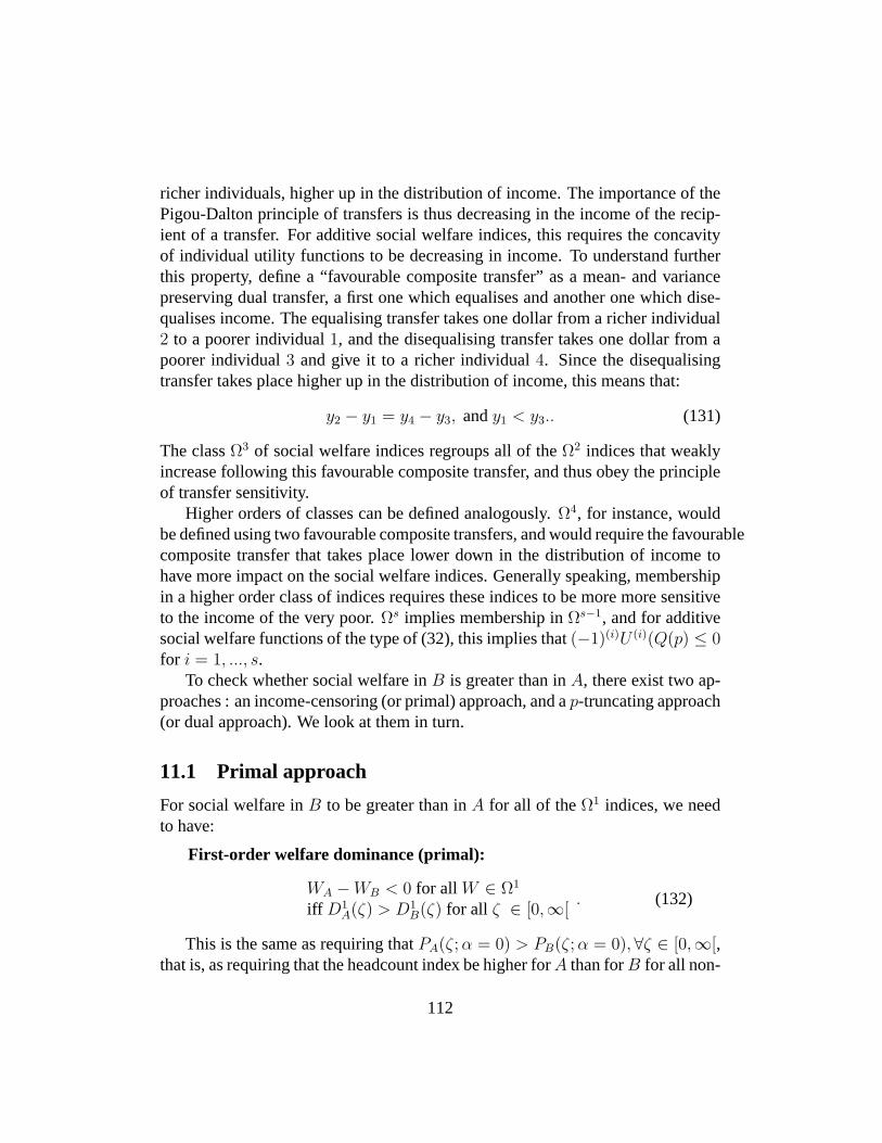
richer individuals, higher up in the distribution of income. The importance of thePigou-Dalton principle of transfers is thus decreasing in the income of the recip-ient of a transfer. For additive social welfare indices, this requires the concavityof individual utility functions to be decreasing in income. To understand furtherthis property, define a “favourable composite transfer” as a mean- and variancepreserving dual transfer, a first one which equalises and another one which dise-qualises income. The equalising transfer takes one dollar from a richer individual2 to a poorer individual1, and the disequalising transfer takes one dollar from apoorer individual3 and give it to a richer individual4. Since the disequalisingtransfer takes place higher up in the distribution of income, this means that:

y2 − y1 = y4 − y3, andy1 < y3.. (131)

The classΩ3 of social welfare indices regroups all of theΩ2 indices that weaklyincrease following this favourable composite transfer, and thus obey the principleof transfer sensitivity.

Higher orders of classes can be defined analogously.Ω4, for instance, wouldbe defined using two favourable composite transfers, and would require the favourablecomposite transfer that takes place lower down in the distribution of income tohave more impact on the social welfare indices. Generally speaking, membershipin a higher order class of indices requires these indices to be more more sensitiveto the income of the very poor.Ωs implies membership inΩs−1, and for additivesocial welfare functions of the type of (32), this implies that(−1)(i)U (i)(Q(p) ≤ 0for i = 1, ..., s.

To check whether social welfare inB is greater than inA, there exist two ap-proaches : an income-censoring (or primal) approach, and ap-truncating approach(or dual approach). We look at them in turn.

11.1 Primal approach

For social welfare inB to be greater than inA for all of theΩ1 indices, we needto have:

First-order welfare dominance (primal):

WA −WB < 0 for all W ∈ Ω1

iff D1A(ζ) > D1

B(ζ) for all ζ ∈ [0,∞[. (132)

This is the same as requiring thatPA(ζ; α = 0) > PB(ζ; α = 0),∀ζ ∈ [0,∞[,that is, as requiring that the headcount index be higher forA than forB for all non-

112

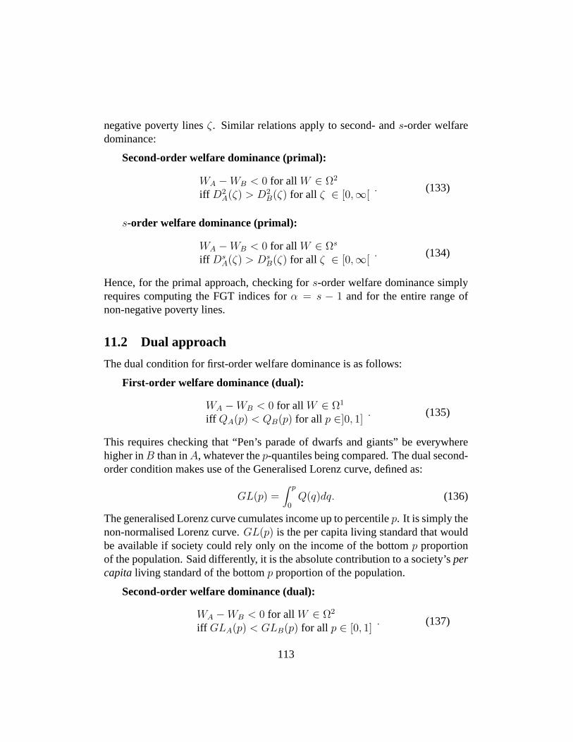
negative poverty linesζ. Similar relations apply to second- ands-order welfaredominance:

Second-order welfare dominance (primal):

WA −WB < 0 for all W ∈ Ω2

iff D2A(ζ) > D2

B(ζ) for all ζ ∈ [0,∞[. (133)

s-order welfare dominance (primal):

WA −WB < 0 for all W ∈ Ωs

iff DsA(ζ) > Ds

B(ζ) for all ζ ∈ [0,∞[. (134)

Hence, for the primal approach, checking fors-order welfare dominance simplyrequires computing the FGT indices forα = s − 1 and for the entire range ofnon-negative poverty lines.

11.2 Dual approach

The dual condition for first-order welfare dominance is as follows:

First-order welfare dominance (dual):

WA −WB < 0 for all W ∈ Ω1

iff QA(p) < QB(p) for all p ∈]0, 1]. (135)

This requires checking that “Pen’s parade of dwarfs and giants” be everywherehigher inB than inA, whatever thep-quantiles being compared. The dual second-order condition makes use of the Generalised Lorenz curve, defined as:

GL(p) =∫ p

0Q(q)dq. (136)

The generalised Lorenz curve cumulates income up to percentilep. It is simply thenon-normalised Lorenz curve.GL(p) is the per capita living standard that wouldbe available if society could rely only on the income of the bottomp proportionof the population. Said differently, it is the absolute contribution to a society’spercapita living standard of the bottomp proportion of the population.

Second-order welfare dominance (dual):

WA −WB < 0 for all W ∈ Ω2

iff GLA(p) < GLB(p) for all p ∈ [0, 1]. (137)

113

Figure24 shows four cases of comparisons of average income and inequalityacross two distributionsA andB. In Case 1,A inequality-dominatesB, and italso has a higher average living standard. Hence, there is generalized-Lorenz-dominance ofA over B. In Case 2,A also inequality-dominatesB accordingto the Lorenz criterion, butµA < µB; GLA(p) crossesGLB(p) and there canbe no unambiguous social welfare ranking. Case 3 depicts an ambiguous rank-ing of inequality acrossA andB. However, becauseµA is well aboveµB, thegeneralized Lorenz curve forA dominates that forB. Finally, Case 4 shows acircumstance in which inequality and social welfare rankings clash.A has unam-biguously less inequality thanB according to the Lorenz criterion, butµA beingsignificantly belowµB, A has unambiguously less social welfare thanB accordingto the generalized-Lorenz criterion.

114

Part IV

Poverty and equity: policy designand assessment

115

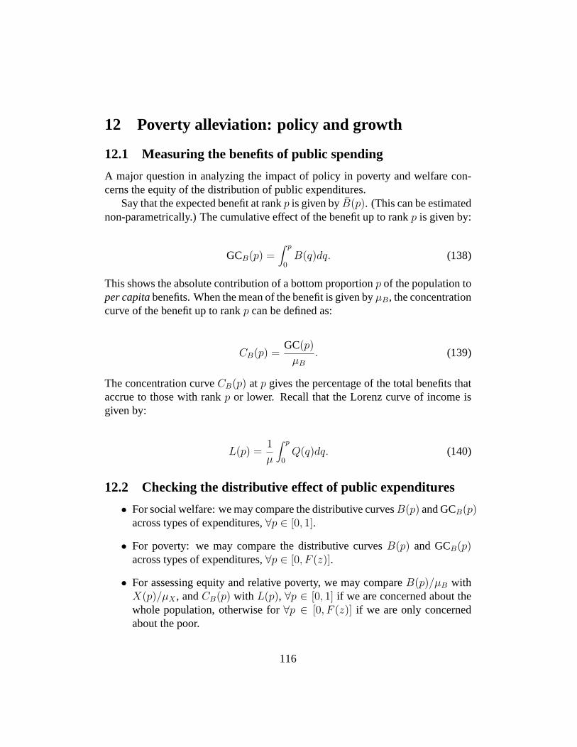
12 Poverty alleviation: policy and growth

12.1 Measuring the benefits of public spending

A major question in analyzing the impact of policy in poverty and welfare con-cerns the equity of the distribution of public expenditures.

Say that the expected benefit at rankp is given byB(p). (This can be estimatednon-parametrically.) The cumulative effect of the benefit up to rankp is given by:

GCB(p) =∫ p

0B(q)dq. (138)

This shows the absolute contribution of a bottom proportionp of the population toper capitabenefits. When the mean of the benefit is given byµB, the concentrationcurve of the benefit up to rankp can be defined as:

CB(p) =GC(p)

µB

. (139)

The concentration curveCB(p) at p gives the percentage of the total benefits thataccrue to those with rankp or lower. Recall that the Lorenz curve of income isgiven by:

L(p) =1

µ

∫ p

0Q(q)dq. (140)

12.2 Checking the distributive effect of public expenditures

• For social welfare: we may compare the distributive curvesB(p) and GCB(p)across types of expenditures,∀p ∈ [0, 1].

• For poverty: we may compare the distributive curvesB(p) and GCB(p)across types of expenditures,∀p ∈ [0, F (z)].

• For assessing equity and relative poverty, we may compareB(p)/µB withX(p)/µX , andCB(p) with L(p), ∀p ∈ [0, 1] if we are concerned about thewhole population, otherwise for∀p ∈ [0, F (z)] if we are only concernedabout the poor.

116

We may also use ”income growth curves”,(N(p) − X(p))/X(p), to detectwhether net incomes are higher than gross (pre-benefit) incomes. This is equiv-alent to graphing changes in quantile curves for net incomes. If growth is every-where positive, absolute poverty must have have been decreased. It the growthcurve for the poor is above mean growth, then the system is ”pro-poor”, in thesense that it increases the incomes of the poor faster than those of the rest of thepopulation. An exactly equivalent test can be done by comparing the normalizedquantiles for gross and net incomes – recall that normalized quantilesQ(p)/µ arejust incomes as a proportion of mean income. If normalized quantiles for the poorare increased by the benefit system, then the system is ”pro-poor”.

Income growth curves may also be used to consider the impact of state benefitsand public expenditures uponrelativepoverty. The procedure is similar to that ofchecking whether the benefit system is pro-poor – we compare income growth forthe poor to the growth of central tendency of the distribution of income for thewhole population. One difference with the measurement of pro-poor growth isthat the central tendency of interest may be median income (or any other quantile)if the relative poverty line is set as a proportion of that median income.

Measuring the benefits of public spending can also be done by assessing byhow much the cumulative income of bottom proportionsp of the poor is affectedby that public spending. If that cumulative income increases for allp lower thanthe initial headcountF (z), then poverty is necessarily reduced by the benefitsof public spending for all distribution-sensitive poverty indices. Further, if thegrowth in the cumulative incomes of the poor is larger than the growth in meanincome, then public spending reduces inequality and enhances for the benefit ofthe poor the vertical equity of the distribution of living standards. It is equivalentto checking whether the Lorenz curve is pushed up by public spending for allpossible cumulative proportions of the poor.

12.3 The impact of targeting and public expenditure reformson poverty

For policy purposes, it is often more useful to assess the impact ofreformsto abenefit or public expenditure system than to evaluate the effect ofexistingsystems.An essential question to answer in the assessment of such reforms is: how will thebenefits of such reforms be spread? There is clearly an infinite number of ways inwhich reforms to the pattern of public expenditures can be made.

We consider five such ”reforms” in this section. The first one channels public

117

expenditure benefits to members of specific and easily observable socio-economicgroups. The main issue then is, ”in which socio-economic group is additionalpublic money best spent to reduce aggregate poverty?” The second type of reformconsists in an increase in public expenditures that raises all incomes in some socio-economic groups by some proportional amount. Again, an important question isfor which socio-economic group this increase of public expenditures would reduceaggregate poverty the fastest. This second type of reform can also be thought asa process that increase the quality of infrastructure and the quantity of economicactivity in a particular group or region – in a way that affects proportionally allincomes and that is thus distributionally neutral in the sense of not affecting in-equality within the groups affected.

The third type of reform considers a change in the price of some commodities,either through some macroeconomic or external shocks, or through a change incommodity taxes or subsidies. How is the distribution of well-being, and povertyin particular, affected by such a price change? The following question we askis: what type of reform to a system of commodity taxes and subsidies could weimplement, with no change in overall government revenues, but with a fall inpoverty? That is, which commodities should be prime targets for a reduction intheir tax rate or for an increase in their rate of subsidy? The fifth and last type ofreform affects proportionally all incomes of a certain type – such as some type offarm income, the labor income of some type of workers,etc...

For all such reforms, we measure their poverty impact by the change in theFGT poverty indices that they cause. Recall also that the use of the FGT povertyindices is closely connected to checks for stochastic dominance and ethical ro-bustness of poverty changes. Hence, we can use the methods below to determinehow the reforms affect poverty as measured not only by the FGT poverty indices,but by all poverty indices which obey some ethical conditions. For instance, ifwe find that some form of targeting decreases a FGT index of someα value for arange[0, z+] of poverty lines, then we know that the reform will also decrease allpoverty indices of ethical orderα + 1, whatever the choice of poverty line within[0, z+].

118

12.3.1 Group-targeting a constant amount

We consider first the effect of a transfer of a constant amount of income to everyone in a groupk. For this, recall that the FGT index can be decomposed as:

P (z; α) =K∑

k=1

φ(k)P (k; z; α). (141)

Theper capitacost to the government of granting anequalamountη(k) to eachmember of a groupk is equal to:

R =K∑

k=1

φ(k)η(k). (142)

Aggregate poverty after such transfers is equal to:

P (k; z; α) =∫ 1

0[z −Q(k; p; z)− η(k)]α+ dp. (143)

To determine which groupk should be of greatest priority for the targeting of gov-ernment expenditures, we need to determine for which groupk government ex-penditures (in the form ofηk) reduce aggregate poverty the most. In other words,we need to compare acrossk the aggregate poverty reduction benefits of targeting$1 to groupk.

Whenα 6= 0, we can show that the marginal reduction of aggregate povertyper dollar ofper capitagovernment expenditures is given by:

∂P (z; α)

∂η(k)/

∂R

∂η(k)= −αP (k; z; α− 1) ≤ 0. (144)

To reduceP (z; α) the most, we must therefore target groups for whichP (k; z; α−1) is the greatest. The greater the value ofα, the greater the chance that we willfavor those groups where extreme poverty is highest.

Whenα = 0, the per dollar reduction of aggregate poverty is given byf(k; z),groupk’s density of income at the poverty line:

∂P (z; α = 0)

∂η(k)/

∂R

∂η(k)= −f(k; z) ≤ 0. (145)

119

We must therefore target those groups with the greatest proportion of peoplejust around the poverty line, regardless of how much poverty there is below thatpoverty line – another consequence of the distributive insensitivity of the head-count index.

12.3.2 Inequality-neutral targeting

Consider now a transfer that is proportional to the incomeQ(k; p; z) of each mem-ber of a groupk. Let this proportional increase beλ(k) − 1. The FGT index forgroupk after such a transfer is then:

P (k; z; α) =∫ 1

0[z −Q(k; p; z) · λ(k)]α+ dp. (146)

The marginal impact of a change inλ(k) is given by

∂P (z; α)

∂λ(k)= αφ(k) [P (k; z; α)− zP (k; z; α− 1)] ≤ 0. (147)

How (147) varies across values ofk depends on two factors. First, there is the fac-tor [P (k; z; α)− zP (k; z; α− 1)]. Groups in which there is a significant presenceof extreme poverty will tend to see theirP (k; z; α) poverty indices fall signifi-cantly withα, thus leading to a large value of[P (k; z; α)− zP (k; z; α− 1)]. Wemay thus expect that theses groups should be a target for government targeting.However, those groups with considerable incidence of extreme poverty are alsothose for which a proportional increase in income has the least impact on the av-erage income of the poor – since there is then little income on which growth maytake effect. Hence, whether those groups with higher incidence of extreme povertywill exhibit a higher value of[P (k; z; α)− zP (k; z; α− 1)] is ambiguous.

The second factor that enters into (147) is population shareφ(k). Ceterisparibus, targeting government expenditures (in the form of an increase inλ(k)) togroups with a high population share will naturally tend to decrease overall povertyfastest. But this fails to take into account that a given increases inλ(k) will gen-erally be more costly for the government to attain for groups with a large share ofthe population. Because of this, we may instead wish to compare across groupsthe ratio of the benefit in poverty reduction to the groupper capita increase inincome. Assume that the cost of this groupper capitaincome increase is entirelyborne by the government. Theper capitarevenue impact of such a transfer on thegovernment budget equals∂R/∂λ(k), where:

120

R = φ(k)µ(k)λ(k). (148)

Whenα 6= 0, the reduction of aggregate poverty per dollarper capitaspent isthen:

∂P (z; α)

∂λ(k)/

∂R

∂λ(k)=

α [P (k; z; α)− zP (k; z; α− 1)]

µ(k)≤ 0. (149)

To reduceP (z; α) the fastest, the government should therefore target those groupsfor which the term on the right is the greatest in absolute value. Compared to(147), (149) does not feature population shares as a factor, since it is cancelled bythe revenue impact of the government transfer. There now appears, however, thetermµ(k) in the denominator. Indeed, if it must bear the entire cost of the incomeincrease, the government will have to pay more to achieve a given increase inλ(k) for those groups with a high average income than for those with a loweraverage income level. Finally, and for the same reasons as above, whether thosegroups with higher incidence of extreme poverty will exhibit a higher value of[P (k; z; α)− zP (k; z; α− 1)] is ambiguous.

Whenα = 0, the per dollar reduction of aggregate poverty from a proportional-to-income transfer is given by

∂P (z; α = 0)

∂λ(k)/

∂R

∂λ(k)= −z · f(k; z)

µ(k)≤ 0. (150)

Those groups with a high density of income at the poverty line, and whoseaverage income is small, are then a prime target for poverty-efficient proportional-to-income transfer scheme.

12.3.3 Price changes

The level of relative prices is an important determinant of the distribution of liv-ing standards, and can therefore matter significantly for poverty analysis. Govern-ments can affect their levels directly or indirectly. Maintaining high import tariffsor failing to implement regulations to foster competition may protect national pro-ducers by maintaining high domestic producer prices, but it will also lead to highconsumption prices, which will hurt consumers. The use of sales and indirect

121

taxes to raise tax revenues also affects relative prices, and thus consumer and pro-ducer well-being. Price subsidies on food, education, energy and transportationare yet another example of government policies which affect relative prices andthus poverty.

To see how changes in relative prices (and therefore how price-changing re-forms) can impact poverty, we denote byy a household-specific level of exoge-nous income, and express consumers’ preferences asϑ . The indirect utility func-tion is given byV (y, q; ϑ), whereq is a vector of consumer and producer prices.We define a vector of reference prices asqR – this is necessary to assess con-sumers’ well-being at constant prices. Denote the real income in the post-reformsituation byyR, whereyR is measured on the basis of the reference pricesqR.yR is implicitly defined byv

(yR, qR; ϑ

)= v (y, q; ϑ), and explicitly by the real

income functionyR = R(y, q, qR; ϑ

), where

V(R

(y, q, qR; ϑ

), qR; ϑ

)≡ V (y, q; ϑ) . (151)

By definition,yR gives the level of income that provides underqR the same realliving standard asy yields underq.

We then wish to determine how real living standards are affected by a marginalchange in prices. Letxc (y, q; ϑ) be the net consumption of goodc (which can benegative if the individual or household is a net producer of goodc) of a con-sumer/producer with incomey, preferencesϑ and facing pricesq. Let qc be theprice of goodc. Using Roy’s identity and setting reference prices to pre-reformprices, we find:

∂R(y, q, qR; ϑ, )

∂qc

∣∣∣∣∣q=qR

=∂V (y, q; ϑ) /∂qc

∂V (yR, qR; ϑ) /∂yR

∣∣∣∣∣q=qR

= − ∂V (y, q; ϑ) /∂y

∂V (yR, qR; ϑ) /∂yR

∣∣∣∣∣q=qR

· xc (y, q; , ϑ)

= −xc

(y, qR; ϑ

). (152)

Equation (152) says that observed pre-reform net consumption of goodc isa sufficient statistic to know the impact on the real living standard of a marginalchange in the price of goodc. This simple relationship is in fact also valid forrationed goods. Equation (152) gives a ”first-order approximation” to the truechange in real income that occurs from a change in the price of goodc. The

122

approximation isexactwhen the price change is marginal. It becomes less exactif the price change is non-marginal and if the compensated demand for goodcvaries significantly withqc.

Assume that preferencesϑ and exogeneous incomey are jointly distributedaccording to the distribution functionF (y, ϑ). The conditional distribution ofϑgiveny is denoted byF (ϑ |y ), and the marginal distribution of incomey is givenby F (y). Let preferences belong to the setΘ, and assume income to be distributedover[0, a]. Expected consumption of goodc at incomey is given byxc(y, q), suchthat

xc(y, q) = Eϑ [xc (y, q; ϑ)] =∫

Ωxc (y, q; ϑ) dF (ϑ|y). (153)

By (152),−xc(y, q) is also proportional to the expected fall in real living standardsof those with incomey that arises from an increase inqc.

Let xc(q) then be theper capitaconsumption of thecth good, defined asxc(q) =

∫ a0 xc (y, q) dF (y) . By (152), xc(q) is also the average welfare cost of

an increase in the price of goodc. As a proportion ofper capitaconsumption,consumption of goodc at incomey is expressed asxc(y, q) = xc(y, q)/xc(q).

It is now at last useful to see how the FGT indicesP (z; α) are affected by achange in the price of goodk10. Using (152), we can show that:

∂P (z; α)

∂qc

∣∣∣∣∣q=qR

=

xc

(z, qR

)f(z), if α = 0

αz−α∫ z0 xc

(y, qR

)(z − y)α−1 dF (y) if α = 1, 2, ...

(154)wheref(z) is again the density of income atz. When the effect on the FGTindices of an increase in the price of a goodc is graphed over a range of povertylinesz, this generates the “consumption dominance”CDc(z; α) curve of goodc:

CDc(z; α) =∂P (z; α)

∂qc

, α = 0, 1, 2, ... (155)

Note that the impact on poverty depends onα andz. By (154), CDc(z; α = 0)only takes into account the consumption pattern of those precisely atz. The im-pact of an increase in the price of goodc on the headcount index will be largeif there are many around the poverty line (f(z) is large) and/or if they consumemuch of goodc (xc

(z, qR

)is large). TheCDc(z; α = 1) curve gives the absolute

contribution to total consumption ofc of those individuals with income less than

10For normalized FGT indices, we simply multiply the results byzα.

123

z. It is therefore an informative statistics on the distribution of consumption ex-penditures, similar in content to the generalized concentration curveGCxc(p) forgoodc – which gives the absolute contribution to totalxc consumption of thosebelow a certain rankp. Forα = 2, 3, ..., progressively greater weight is given forthe computationCDc(z; α) to the shares of those with higher poverty gaps.

12.3.4 Tax/subsidy policy reform

The above section gave us the tools needed to assess the impact of marginal pricechanges on poverty. We may now use these tools to assess whether a revenue-neutral tax and subsidy reform could be implemented that would reduce aggregatepoverty.

For this, we need to consider the government budget constraint, and more par-ticularly the net revenues that the government raises from its policy of commoditytaxes and subsidies. Setting producer prices to1 and assuming them for simplicityto be constant and invariant to changes int, the vector of tax rates on theC goods,we then haveq = 1 + t anddqc = dtc, whereqc andtc denote respectively theconsumer price of and the tax rate on goodc. Let per capita net commodity taxrevenues be denoted asR(q). They are equal toR(q) =

∑Cc=1 tcxc(q). Without

loss of generality, assume that the government’s tax reform increases the tax rateon thejth commodity and uses the proceeds to decrease the tax rate (or to increasethe subsidy) on thelth commodity. Revenue neutrality (a conventional assumptionin the optimal taxation literature) of the tax reform requires that

dR(q) =

[xj(q) +

C∑

c=1

tc∂xc(q)

∂qj

]dqj +

[xl(q) +

C∑

c=1

tc∂xc(q)

∂ql

]dql = 0. (156)

Defineγ as

γ =xl(q) +

∑Cc=1 tc

∂xc(q)∂ql

xl(q)

/xj(q) +

∑Cc=1 tc

∂xc(q)∂qj

xj(q), (157)

The numerator in (157) gives the marginal tax revenue of a marginal increasein the price of goodl, per unit of the average welfare cost that this price increaseimposes on consumers. Equivalently, this is1 minus the deadweight loss of taxinggoodl, or the inverse of the marginal cost of public funds (MCPF) from taxingl(see Wildasin (1984)). The denominator gives exactly the same measures for anincrease in the price of goodj. γ is thus the economic (or “average”) efficiency oftaxing goodl relative to taxing goodj. We may thus interpretγ as the efficiency

124

cost of taxingj relative to that of taxingl (the MCPF forj over that forl). Thehigher the value ofγ, the less economically efficient is taxing goodj.

By simple algebraic manipulation, we can then rewrite equation (156) as

dqj = −γ

(xl(q)

xj(q)

)dql, (158)

which fixesdqj as a revenue-neutral proportion ofdql. This last relationship givesus a nice synthetic expression for the impact on a FGT indexP (z; α) of a revenue-neutral tax reform that increases the tax on a goodl for a benefit of a fall in thetax on a goodj:

∂P (z; α)

∂tl

∣∣∣∣∣revenue neutrality= CDl(z; α)− γxl(q)CDj(z; α)/xj(q), . (159)

As mentioned above, we may wish to check whether such a tax reform wouldlead to an ”ethically robust” fall in poverty, namely, that poverty would fall asmeasured by any one of the poverty indices of some ethical order and for a rangeof poverty lines. To do this, it is useful to define and use normalizedCD curves,denoted asCDc(z; α). NormalizedCD curves are just the above-definedCDcurves for goodc normalized by the average consumption of that good,xc(q):

CDc(z; α) =CDc(z; α)

xc(q). (160)

CD curves are thus the ethically weighted (or social) cost of taxingc as a propor-tion of the average welfare cost. Comparing normalizedCDc(z; α) curves allowsus to compare the distributive benefits of decreasing tax rates (or increasing subsi-dies) across commodities. IfCDl(z; α) > CDj(z; α) ≥ 0, then investing 1 dollarof public expenditures to decrease the burden of taxation onl will have a greaterdistributive benefit (will lead to greater poverty reduction) than for commodityj.

For overall social efficiency, we must also take into the parameter of economicefficiency,γ. We may check whether a tax reform is ”poverty efficient” by veri-fying whether the following condition holds:

CDl(z; α)− γCDj(z; α) ≥ 0,∀z ∈[0, z+

]. (161)

If condition (161) holds, then it iss-order poverty efficient (wheres = α + 1) todecreasethe tax on goodl for a revenue-neutral benefit of anincreasein the taxon goodj. Poverty will decrease following this tax reform for all poverty indicesof thes order and for all poverty lines within[0, z+].

125

12.3.5 Income-component and sectoral growth

It is just a matter of notational change to use the tools developed above to assessthe poverty impact of growth in some income component or in some sector ofeconomic activity. We may assess, for instance, by how much would aggregatepoverty fall per percentage of growth in the industrialized sector, or per dollar ofgrowth in agricultural income (an income component that enters into aggregateincome).

Assume that total incomeX is the sum ofC income components, withX =∑Cc=1 λcXc, and whereλc is a factor that multiplies income componentc and that

can be subject to growth. The derivative of the normalized FGT with respect toλc

is given by

∂PX(z; α)

∂λc

∣∣∣∣∣λc=1,c=1,...,C

= CDc(z; α), (162)

where thisCDc(z; α) curve is now a ”component dominance” curve for incomecomponent or for sectoral incomeXc. Multiplied by a proportional changedλc,CDc(z; α) will give us the marginal change in the FGT indices that we can expectfrom growth in sector or in componentc.

We can reasonably expect, however, that a given percentage change in a largesector or for a large income component will have a larger impact on poverty thanotherwise. To take this factor into account, we may wish instead to compute thechange in the FGT indicesper dollar of per capitagrowth. This is given by thenormalizedCD curves for componentc:

∂P (z; α)/∂λc

∂µX/∂λc

∣∣∣∣∣λc=1,c=1,...,C

= CDc(z; α). (163)

Finally, we may wish to compute theelasticityof poverty with respect to over-all growth, where again that overall growth comes strictly from growth in a com-ponentXc. From (163), this is given by:

∂P (z;α)/∂λc

∂µX/∂λc

∣∣∣∣λc=1,c=1,...,C

P (z; α)/µX

=CDc(z; α)

P (z; α)· µX . (164)

12.4 Overall growth elasticity of poverty

How fast can inequality-neutral growth in the economy be expected to reducepoverty? From which group inequality-neutral growth can be expected to reduce

126

aggregate poverty the fastest? And in which group would poverty fall the fastestdue to such growth?

Using (147) above, it can be shown that the elasticity of total povertyP (z; α)with respect to total income – when growth in total income comes exclusivelyfrom inequality-neutral growth in groupk – equals

εy(k; z; α) =α [P (k; z; α)− zP (k; z; α− 1)]

P (z; α)(165)

for α 6= 0. As discussed above, it is ambiguous whether growth in groups with sig-nificant incidence of extreme poverty would be those whose growth would be mostbeneficial for overall poverty reduction. ReplacingP (k; z; α) andP (k; z; α − 1)by P (z; α) andP (z; α − 1) respectively gives as a special case the elasticity ofpoverty with respect to inequality-neutral growth in the overall economy,εy(z; α).ReplacingP (z; α) by P (k; z; α) provides as another special case the elasticity ofpoverty in groupk with respect to inequality-neutral growth in that same group.

Whenα = 0, (165) becomes:

εy(k; z; α = 0) =−zf(k; z)

F (z). (166)

This expression has a nice graphical interpretation. To see this, consider Fig-ure30 where the densityf(y) of income at differenty is shown. Recall that thearea underneath thef(y) curve up toy = z gives the headcountF (z). The termz ·f(k; z) in (166) is the area in Figure30of the rectangle with widthz and heightf(z). Hence, the elasticity (in absolute value) of the headcount with respect toinequality-neutral growth is given in Figure30by the ratio of the rectangular areaz · f(k; z) over the shaded areaF (z).

It is clear, then, that this elasticity is larger than one whenever the poverty linez is lower than the (first) mode of the distribution. In fact, it will be above one inFigure30 for any poverty line up to approximativelyz′. For poverty lines largerthanz′, the growth elasticity will in absolute value fall below 1. This can haveimportant policy consequences. For societies in which the poverty line is deemedto be lower than the mode (which is usually not far from the median), then theheadcount in these societies will fall at a proportional rate that is faster than thegrowth rate in average living standards. But for societies in which the headcountis initially high (larger than 0.5, say), we can expect the growth elasticity of the

127

headcount to be lower than 1. This means that inequality-neutral growth can beexpected to have a proportionately smaller impact on the number of the poor inpoorer societies than in richer ones.

12.5 The Gini elasticity of poverty

It may also be of interest to predict how changes in inequality will affect poverty.The difficulty is that, unlike for the case of growth in mean income, it is notobvious which pattern of changing inequality we should consider. As discussedabove, a natural reference case for analyzing the impact of growth is the case ofinequality-neutral growth – all incomes vary proportionately by the same growthrate in mean income. For inequality changes, which inequality measure should weuse? And even if we were to agree on the choice of one single summary inequalityindex, there are many different ways in which a given change in such an index maybe obtained, even keeping mean income constant. And these different ways couldalso have a dramatically different impact on poverty.

So trying to predict the effect on poverty of a process of changing inequality,through the use of a single indicator of inequality, is really to ask too much ofsummary indices of inequality. There cannot exist any stable structural relation-ship between inequality indices and poverty, even keeping mean income constant.This casts severe doubt on the structural validity of the many studies that regresschanges in poverty indices upon changes in inequality indices.

What can be done, however, is toillustrate how some peculiar and simplisticpattern of changing inequality can affect poverty. Such an illustration can be madeusing the single-parameter (λ) process of bi-polarization shown by equation (17).How does poverty change when inequality changes due to this bi-polarization?For this, we use the most popular indices of poverty and inequality, the FGT andthe Gini indices (the result is exactly the same for the broader class of S-Giniindices). The elasticity of poverty with respect to the Gini index – when changinginequality comes from aλ that moves marginally away from 1– is given whenα > 0 by

εG(z; α) = α

(1 +

P (z; α− 1)

P (z; α)(µ− z)

)(167)

for the un-normalized FGT indices, and by

εG(z; α) =

(1 +

P (z; α− 1)

P (z; α)

(µ

z− z

))(168)

128

for the normalized FGT. When the headcount is used, we obtain

εG(z; α = 0) = f(z) (µ− z) . (169)

Note that even with this highly simplified process of changing inequality, theimpact of changing inequality on poverty is ambiguous. It depends in part on thesign of(µ− z). When mean income is below the poverty line, an increase in theGini index can – and, for the headcount index,will – mean afall in poverty.

13 The impact of policy and growth on inequality

13.1 Growth, tax and transfer policy, and price shocks

We may now turn to the impact of policy and growth on inequality. The approachwe will use will enable us to consider the impact on inequality of several waysin which income changes may occur. One is growth that takes place within aparticular socio-economic group. Another is growth that affects the value of someincome sources – such as agricultural income of informal urban labor income. An-other is the impact of price changes, which affect real income and its distribution.One more is the impact of changes in some tax or benefit policies, such as chang-ing the subsidy rates on some production or consumption activity, or increasingthe amount of monetary transfers made to some socio-economic groups.

For each such income-changing phenomenon, we may be interested in theabsolute amount by which inequality will change, or in the absolute amount bywhich inequality will change for each percentage change in mean real income, orin the elasticity of inequality with respect to mean income.

Assume that we have as above that total standard of livingX is the sum ofCcomponents,X =

∑Cc=1 λcXc, to which we apply again a factorλc. We then have

thatµX =∑C

c=1 λcµXc . If we are interested in total consumption, then we maythink of theXc as different types of consumption expenditures. If we are thinkingof tax and benefit policy, then some of theXc may be transfers or taxes. If we arealternatively concerned with the impact of sectoral growth on income inequality,then we may think of theXc as different sources of income, or of the income ofdifferent socio-economic groups. By how much, then, is inequality affected byvariations inλc?

We will consider two ways of measuring inequality, the Lorenz curve and theS-Gini inequality indices – of which the traditional Gini is again a special case.The derivative of the Lorenz curve ofX with respect toλc is given by:

129

∂LX(p)

∂λc

∣∣∣∣∣λc=1,c=1,...,C

=µXc

µX

(CXc(p)− LX(p)) . (170)

(170) therefore gives the change in the Lorenz curve per 100% proportional changein the value ofXc. Say that we predict that income componentXc will increaseby approximately by 10% over the next year. Then we can predict that the LorenzcurveLX(p) will move by approximately10% · µXc/µX (CXc(p)− LX(p)) overthat same period. How big an impact this will be on inequality will depend on thesize of the proportional change, on the importance of the component (µXc), andon the concentration of the component relative to that of total living standards (thedifferenceCXc(p)− LX(p)).

A similar result is obtained for the Gini indices:

∂IX(ρ)

∂λc

∣∣∣∣∣λc=1,c=1,...,C

=µXc

µX

(ICXc(ρ)− IX(ρ)) . (171)

Thus, if for instance the removal of a subsidy or the advent of an external shockis foreseen to increase by 10% the price of a goodXc, the Gini index can be pre-dicted to move by approximately− [10% · µXc/µX (CXc(p)− LX(p))] (the neg-ative sign comes from the fact that an increase in the price of a consumption goodleads to a fall in the real value of the expenditures made on that good).

We may also wish to assess the impact on inequality per 100% of mean incomechange. This is given by

µX∂LX(p)/∂λc

∂µX/∂λc

∣∣∣∣∣λc=1,c=1,...,C

= CXc(p)− LX(p) (172)

for the Lorenz curve and by

µX∂IX(ρ)/∂λc

∂µX/∂λc

∣∣∣∣∣λc=1,c=1,...,C

= ICXc(ρ)− IX(ρ) (173)

for the Gini indices. Multiplying the above two expressions by the proportionalimpact that some change inXc is predicted to have on totalper capitaincome willgive the predicted absolute change in inequality. For instance, if we predict thatgrowth in rural areas will lift mean income in a country by 5%, then the Lorenzcurve of total income atp will shift by approximately0.05 (CXc(p)− LX(p)),whereXc is rural income.

130

Finally, it may be preferred to know the elasticity of inequality with respect toµX , when growth comes entirely fromXc. It is given by

CXc(p)

LX

(p)− 1 (174)

for the Lorenz curve and by

ICXc(ρ)

IX(ρ)− 1 (175)

for the Gini indices. Thus, an increase in taxes on formal labor income that reducetotal mean income (net of taxes) by 1 percent will change the Gini index by1 −ICXc(ρ)/IX(ρ) percent.

13.2 Tax and subsidy reform

As in the case of poverty, it is useful to assess the impact of a price reform (throughconsumption and production taxation) on inequality. Assume that we are inter-ested in the effects of a revenue-neutral tax reform that increases the tax on agood l for a benefit of a fall in the tax on a goodj. Recall thatγ is the MCPFfor j over that forl – the larger the value ofγ, the larger the fall intj that we cangenerate for a given revenue-neutral increase intl. A 100% increase in the priceof goodl then has the following impact

∂LX(p)

∂tl

∣∣∣∣∣revenue neutrality=

µxl(q)

µX

[γ

(CXj

(p)− LX(p))− (CXl

(p)− LX(p))]

(176)on the Lorenz curve and

∂IX(ρ)

∂tl

∣∣∣∣∣revenue neutrality=

µxl(q)

µX

[γ

(ICXj

(ρ)− IX(ρ))− (ICXl

(ρ)− IX(ρ))]

(177)for the Gini indices. Whenγ = 1, viz, when the relative economic efficiencyof taxing l or j is not of concern, then expressions (176) and (177) reduce to amultiple of the difference between the concentration curves and the concentrationindices for the two goods. It is then better for inequality reduction to tax more thegood less concentrated among the poor for the benefit of a reduction in the tax rateon the other good, less concentrated among the rich. Changes in the value ofγ

131

may sometimes change the good whose tax rate should be increased for inequalityreduction. We may also wish to express the above changes in inequality per 100%change in the value ofper capitareal income. This is then given by

γ(CXj

(p)− LX(p))− (CXl

(p)− LX(p)) (178)

on the Lorenz curve and

γ(ICXj

(ρ)− IX(ρ))− (ICXl

(ρ)− IX(ρ)) (179)

for the Gini indices.

132

Part V

Estimation and inference fordistributive analysis

133

14 Non parametric estimation for distributive anal-ysis

14.1 Density estimation

14.1.1 Univariate density estimation

The use ofnon-parametricdensity estimation procedures for distributive analysishas grown significantly in the last fifteen years or so11. Before then, a significantliterature had developed on the estimation ofparametricmodels of the distribu-tions of income. These models assumed that the distribution of income followeda particular functional form with unknown parameters, such as the log-normal,the Pareto, or variants of the beta or gamma distributions. A major aim was thento estimate the unknown parameters of that functional form, and to test whethera given functional form appeared to estimate better the density of income thananother functional form.

Non-parametric density estimation does not start by positing a functional formfor the distribution of income. Instead, it lets the ”data speak for themselves”.The method is most easily understood by starting with a review of the densityestimation provided by traditional histograms. Histograms provide an estimate ofthe density of a variabley by counting how many observations fall into bins, andby dividing that number by the width of the bin times the number of observationsin the sample. To see this more precisely, denote the origin of the bins byy0 andthe bins of the histogram by[y0 + mh, y0 + (m + 1)h] for positive or negativeintegersm. For instance, if we takem = 0, then the bin is described by theinterval ranging from the origin to the origin plush. The value of the histogramover each of these bins is then defined by

f(y) =(# of Yi in same bin asy)

n · (width of bin containingy). (180)

Such a histogram is shown on Figure26by the rectangles of varying heights overidentical widths, starting with originy0. For bins defined by[y0 + mh, y0 + (m +1)h], the bin width is a constant set toh, but we can also allow the widths tovary across the bins of the histogram. The choice ofh controls the amount ofsmoothingperformed by the histogram. A small bin width will lead to significantfluctuations in the value of the histogram across theh, and a very large width

11This section draws significantly from Silverman (1986), to which readers are referred for moredetails and in-depth analysis.

134

will set the histogram to the constanth−1. Choosing an appropriate value forsuch a smoothing parameter is in fact a pervasive preoccupation in non-parametricestimation procedures, as we will discuss later. The choice of the origin can alsobe important, especially whenn is not very large. There can be, however, littleguidance on that latter choice, except perhaps when the nature of the data suggesta natural value fory0. One way to avoid choosing such ay0 is by constructingwhat will appear soon to be a ”naive” kernel density estimator, that is, one inwhich the pointy in f(y) is always at the center of the bin:

f(y) = (2hn)−1 (# of Yi falling in [y − h, y + h]). (181)

This naive estimator can also be obtained from the use of a weight functionw(u), defined as:

w(u) =

0.5 if |u| < 10 otherwise

(182)

and by defining

f(y) = (nh)−1n∑

i=1

w(

y − Yi

h

). (183)

This frees the density estimation from the choice ofy0. For the estimation of thenaive density estimator, each observationYi provides a ”box” of width2h andheight 0.5 that is centered atYi. f(y) over a range ofy is just the sum of thesenboxes over that range. Because such boxes are not continuous, their sumf(y) willalso be discontinuous, just like the traditional histogram. There will be ”jumps”in f(y) at the pointsYi±h, making this density estimator expositionally unattrac-tive. The naive estimator can also be improved statistically by choosing weightingfunctions that are smoother thanw(u). For this, we can think of replacing theweight functionw(u) by a general ”kernel function”K(u), such that

f(y) = (nh)−1n∑

i=1

K(

y − Yi

h

). (184)

A smooth kernel estimate of the density function that generated the histogram isshown on Figure26.

In general, we would wish∫∞−∞ K(u)du = 1, since then

∫∞−∞ f(y)dy = 1.

For f(y) to qualify fully as a probability density function, we would also requireK(u) ≥ 0 since we would then be guaranteed thatf(y) ≥ 0, although thereare sometimes reasons to allow for negativity of the kernel function.h is usually

135

referred to as the window width, the bandwidth or the smoothing parameter ofkernel estimation procedures. There are also arguments to adjust the windowwidth that applies for observationYi to the number of observations that surroundYi, makingh larger for areas where there are fewer observations12. As for the naivedensity estimator, each observation will provide a box or a ”bump” to the densityestimation off(y), and that bump will have a shape and a width determined bythe shape ofK(u) and the size ofh respectively.

The definition off(y) in (184) makes it inherit the continuity and differen-tiability properties ofK(u). It is often sound and convenient to choose a kernelfunction that is symmetric around 0, with

∫K(u)du = 1,

∫uK(u)du = 0 and

u2K(u)du = σ2K > 0. One such kernel function that has nice continuity and

differentiability properties is the Gaussian kernel, defined by

K(u) = (2π)−0.5 exp−0.5u2

. (185)

The ”bumps” provided by the Gaussian kernel have the familiar bell shapes, aresmoothly differentiable up to any desired level, and are such thatσ2

K = 1.

14.1.2 Statistical properties of kernel density estimation

The efficiency of non-parametric estimation procedures can be measured naturallyby themean square error(MSE) that there is in estimating a function at a pointy.The MSE in estimatingf(y) is defined by

MSEy

(f

)= E

[(f(y)− f(y)

)2]. (186)

The most common way of defining a measure ofglobalaccuracy simply sums themean square error across values ofy. This yields themean integrated square error(or MISE), a measure of the accuracy of estimatingf(y) over the whole range ofy:

MISE(f

)=

∫MSEy

(f

)dy = E

[∫ (f(y)− f(y)

)2dy

]. (187)

The relative efficiency of a particular choice of a kernel functionK(u) canthen be assessed relative to that choice of the kernel function which would mini-mize the MISE. The Gaussian kernel function has very good efficiency properties,although they are not quite as good as some other (less smooth) kernel functions,

12This is done for instance by the nearest neighbor and the adaptive kernel methods.

136

such as the (efficiency-optimal) Epanechnikov, the biweight or the triangular ker-nels, which are described and discussed for instance in Silverman (1986) (see inparticular Table 3.1).

14.1.3 Choosing a window width

Even, however, if we were to agree on a particular shape for an observation-centered kernel function, there would still remain the question of which windowwidth to choose. Again, conditional on the choice of a particular form forK(u),we can choose the window width that minimizes the MISE. To see what this im-plies, note first that we can decompose the MSE aty as a sum of the squared ofthe bias and of the variance that there is in estimatingf(y):

MSEy

(f

)=

[E

(f(y)− f(y)

)2]

+ varf(y). (188)

For symmetric kernel functions, the bias can be shown to be approximately equalto

0.5h2σ2Kf (2)(y), (189)

and the variance to:

n−1h−1f(y)cK . (190)

wherecK =∫

K(u)2du. Substituting (189) and (190) in (188) then gives:

MSEy

(f

)= 0.5h2σ2

Kf (2)(y) + n−1h−1f(y)cK . (191)

Hence, considering (189), we find that the bias off(y) will be low if the kernelfunction has a low variance, since it is then the observations that are ”closer” toy that will count more, and it is those observations that provide the least biasedestimate of the density aty. But the bias also depends on the curvature off(y):in the absence of such a curvature, the density function is linear and the biasprovided by using observations on the left ofy is just (locally) outweighed by thebias provided by using observations on the right ofy. Looking at (190), we findthat a flatter kernel (with a lowercK) decreases the variance off(y), since theestimator is then more equally dependent on the value of the sample observations.We also obtain the familiar result that the variance of the estimator decreasesproportionately with the size of the sample.

137

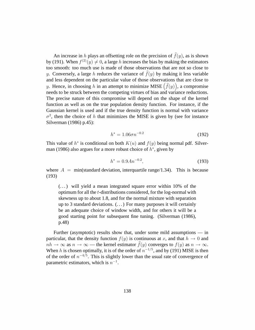
An increase inh plays an offsetting role on the precision off(y), as is shownby (191). Whenf (2)(y) 6= 0, a largeh increases the bias by making the estimatorstoo smooth: too much use is made of those observations that are not so close toy. Conversely, a largeh reduces the variance off(y) by making it less variableand less dependent on the particular value of those observations that are close toy. Hence, in choosingh in an attempt to minimize MISE

(f(y)

), a compromise

needs to be struck between the competing virtues of bias and variance reductions.The precise nature of this compromise will depend on the shape of the kernelfunction as well as on the true population density function. For instance, if theGaussian kernel is used and if the true density function is normal with varianceσ2, then the choice ofh that minimizes the MISE is given by (see for instanceSilverman (1986) p.45):

h∗ = 1.06σn−0.2 (192)

This value ofh∗ is conditional on bothK(u) andf(y) being normal pdf. Silver-man (1986) also argues for a more robust choice ofh∗, given by

h∗ = 0.9An−0.2, (193)

whereA = min(standard deviation, interquartile range/1.34). This is because(193)

(. . . ) will yield a mean integrated square error within 10% of theoptimum for all thet-distributions considered, for the log-normal withskewness up to about 1.8, and for the normal mixture with separationup to 3 standard deviations. (. . . ) For many purposes it will certainlybe an adequate choice of window width, and for others it will be agood starting point for subsequent fine tuning. (Silverman (1986),p.48)

Further (asymptotic) results show that, under some mild assumptions — inparticular, that the density functionf(y) is continuous atx, and thath → 0 andnh → ∞ asn → ∞ — the kernel estimatorf(y) converges tof(y) asn → ∞.Whenh is chosen optimally, it is of the order ofn−1/5, and by (191) MISE is thenof the order ofn−4/5. This is slightly lower than the usual rate of convergence ofparametric estimators, which isn−1.

138

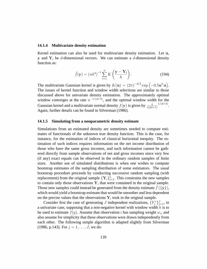
14.1.4 Multivariate density estimation

Kernel estimation can also be used for multivariate density estimation. Letu,y andYi be d-dimensional vectors. We can estimate ad-dimensional densityfunction as:

f(y) = (nhd)−1

n∑

i=1

K

(y −Yi

h

). (194)

The multivariate Gaussian kernel is given byK(u) = (2π)−d/2 exp(−0.5uTu

).

The issues of kernel function and window width selections are similar to thosediscussed above for univariate density estimation. The approximately optimalwindow converges at the raten−1/(d+4), and the optimal window width for theGaussian kernel and a multivariate normal densityf(y) is given by 4

n(2d+1)

1/(d+4).

Again, further details can be found in Silverman (1986).

14.1.5 Simulating from a nonparametric density estimate

Simulations from an estimated density are sometimes needed to compute esti-mates of functionals of the unknown true density function. This is the case, forinstance, for the estimation of indices of classical horizontal inequity. The es-timation of such indices requires information on the net income distribution ofthose who have the same gross incomes, and such information cannot be gath-ered directly from sample observations of net and gross incomes since very few(if any) exact equals can be observed in the ordinary random samples of finitesizes. Another use of simulated distributions is when one wishes to computebootstrap estimates of the sampling distribution of some estimators. The usualbootstrap procedure proceeds by conducting successive random sampling (withreplacement) from the original sampleYin

i=1. This constrains the new samplesto contain only those observationsYi that were contained in the original sample.Those new samples could instead be generated from the density estimatef (y),which would yield a bootstrap estimate that would be smoother and less dependenton the precise values that the observationsYi took in the original sample.

Consider first the case of generatingJ independent realizations,Y ∗j J

j=1, ina univariate case, supposing that a non-negative kernel with window widthh is tobe used to estimatef(y). Assume that observationi has sampling weightwi, andalso assume for simplicity that these observations were drawn independently fromeach other. The following simple algorithm is adapted slightly from Silverman(1986, p.143). Forj = 1, . . . , J , we do:

139

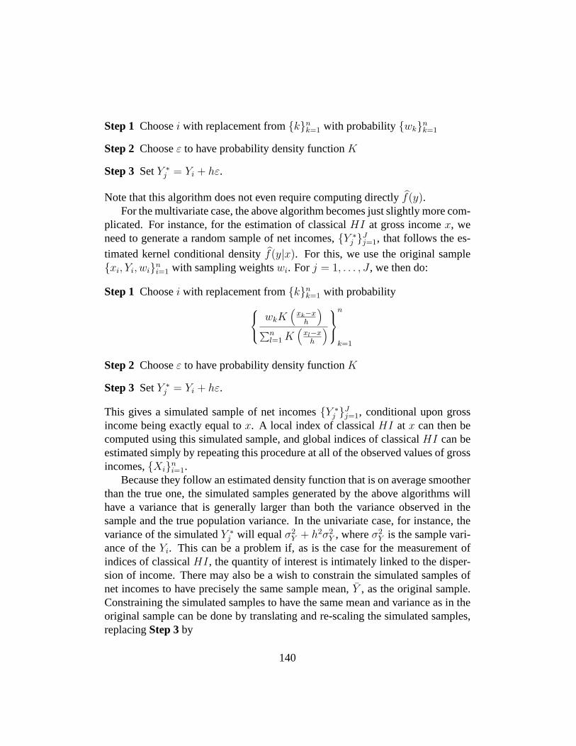
Step 1 Choosei with replacement fromknk=1 with probabilitywkn

k=1

Step 2 Chooseε to have probability density functionK

Step 3 SetY ∗j = Yi + hε.

Note that this algorithm does not even require computing directlyf(y).For the multivariate case, the above algorithm becomes just slightly more com-

plicated. For instance, for the estimation of classicalHI at gross incomex, weneed to generate a random sample of net incomes,Y ∗

j Jj=1, that follows the es-

timated kernel conditional densityf(y|x). For this, we use the original samplexi, Yi, win

i=1 with sampling weightswi. Forj = 1, . . . , J , we then do:

Step 1 Choosei with replacement fromknk=1 with probability

wkK(

xk−xh

)

∑nl=1 K

(xl−x

h

)

n

k=1

Step 2 Chooseε to have probability density functionK

Step 3 SetY ∗j = Yi + hε.

This gives a simulated sample of net incomesY ∗j J

j=1, conditional upon grossincome being exactly equal tox. A local index of classicalHI at x can then becomputed using this simulated sample, and global indices of classicalHI can beestimated simply by repeating this procedure at all of the observed values of grossincomes,Xin

i=1.Because they follow an estimated density function that is on average smoother

than the true one, the simulated samples generated by the above algorithms willhave a variance that is generally larger than both the variance observed in thesample and the true population variance. In the univariate case, for instance, thevariance of the simulatedY ∗

j will equalσ2Y + h2σ2

Y , whereσ2Y is the sample vari-

ance of theYi. This can be a problem if, as is the case for the measurement ofindices of classicalHI, the quantity of interest is intimately linked to the disper-sion of income. There may also be a wish to constrain the simulated samples ofnet incomes to have precisely the same sample mean,Y , as the original sample.Constraining the simulated samples to have the same mean and variance as in theoriginal sample can be done by translating and re-scaling the simulated samples,replacingStep 3by

140

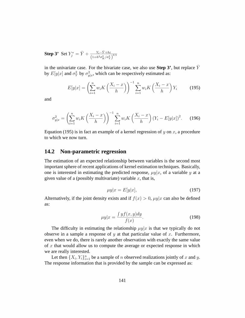
Step 3’ SetY ∗j = Y + Yi−Y +hε

(1+h2σ2K/σ2

Y )0.5

in the univariate case. For the bivariate case, we also useStep 3’, but replaceYby E[y|x] andσ2

Y by σ2y|x, which can be respectively estimated as:

E[y|x] =

(n∑

i=1

wiK(

Xi − x

h

))−1 n∑

i=1

wiK(

Xi − x

h

)Yi (195)

and

σ2y|x =

(n∑

i=1

wiK(

Xi − x

h

))−1 n∑

i=1

wiK(

Xi − x

h

)(Yi − E[y|x])2. (196)

Equation (195) is in fact an example of a kernel regression ofy onx, a procedureto which we now turn.

14.2 Non-parametric regression

The estimation of an expected relationship between variables is the second mostimportant sphere of recent applications of kernel estimation techniques. Basically,one is interested in estimating the predicted response,µy|x, of a variabley at agiven value of a (possibly multivariate) variablex, that is,

µy|x = E[y|x], (197)

Alternatively, if the joint density exists and iff(x) > 0, µy|x can also be definedas:

µy|x =

∫yf(x, y)dy

f(x). (198)

The difficulty in estimating the relationshipµy|x is that we typically do notobserve in a sample a response ofy at that particular value ofx. Furthermore,even when we do, there is rarely another observation with exactly the same valueof x that would allow us to compute the average or expected response in whichwe are really interested.

Let thenXi, Yini=1 be a sample ofn observed realizations jointly ofx andy.

The response information that is provided by the sample can be expressed as:

141

Yi = m(Xi) + εi , whereE[εi] = 0. (199)

To estimateµy|x, kernel regression techniques use a local averaging procedurethat involve weightsK(u) that are analogous to those used in section14.1for den-sity estimation. Recalling (184) and (198), this leads to the following Nadaraya-Watson non-parametric estimator ofµy|x:

m(x) =(nhf(x)

)−1n∑

i=1

K(

x−Xi

h

)Yi

=

∑ni=1 K

(x−Xi

h

)Yi

∑ni=1 K

(x−Xi

h

) . (200)

To reduce the bias of using neighboringYi, the kernel weightsK(

x−Xi

h

)are typ-

ically inversely proportional to the distance betweenx andXi. They also dependon the window widthh.

As for the kernel density estimators, the kernel smootherµy|x can be shownto be consistent under relatively weak conditions, including thatµy|x andf(x)are continuous functions ofx, and thath → 0 andnh → ∞ asn → ∞; seefor instance Hardle (1990), Proposition 3.1.1. Again, the variance ofµy|x alonedoes not fully capture the convergence ofµy|x to µy|x since we must also takeinto account the bias ofµy|x, which comes from the smoothing of theYi in (200).Under suitable regularity conditions, including thath ∼ n−0.2, the asymptotic dis-tribution of the kernel estimator(nh)0.5 (µy|x− µy|x) can be shown to be normal,with its center shifted by its asymptotic bias13. This asymptotic bias is a functionof the form of the kernelK(u) and of the derivatives ofµy|x andf(x). It is givenby:

σ2K

(m(2)(x) + 2m(1)(x)f (1)(x)/f(x)

). (201)

This asymptotic bias can be estimated consistently using estimates ofm(2)(x),m(1)(x), f (1)(x) andf(x). This, however, complicates significantly the computa-tion of the sampling distribution ofµy|x, and it can be avoided if we can expect(or make) the bias to be small compared to the variance. This will be the case ifµy|x is relatively constant, or if we makeh fall just a bit faster than its optimalspeed ofn−0.2; see the discussion of this in Hardle (1990), pp.100–102.

13See Hardle (1990), Theorem 4.2.1, for a demonstration.

142

The variance of(nh)0.5 (µy|x− µy|x) is given by:

σ2y|xcK/f(x). (202)

The conditional varianceσ2y|x can be estimated consistently as in (196). As for

kernel density estimation, note again that the smoothing process makes the rateof convergence of kernel estimatorµy|x to ben−0.4, instead of the usual slightlyfaster parametric convergence rate ofn−0.5.

143

15 Symbols

• y: living standards or income

• yR: ”real” income

• yi: living standard ofith ordered observation

• n: number of observations

• M : household size

• MA: number of adults in household

• E(·): equivalence scale

• s: equivalence scale parameter

• c: equivalence scale parameter

• wi: sampling weight of observationi

• p: percentile

• pi: sample percentile ofith ordered observation

• F (y): distribution function

• f(y): density function

• Q(p): p-quantile

• ymax: maximum income

• µ: mean living standard

• z: poverty line

• Q∗(p; z): p-quantile censored atz

• g(p; z): poverty gap

• µ∗(z): mean of censored income

• µg(z): average poverty gap

144

• L(p): Lorenz curve

• GL(p): generalised Lorenz curve

• G(p; z): Cumulative Poverty Gap (CPG) curve

• κ(p): weight used in linear indices

• κ(p; ρ): weight used in S-Gini indices

• ω(p): weight on income used in linear indices

• ω(p; ρ): weight on income used in S-Gini indices

• I(ρ): S-Gini inequality indices

• δ(p, q): relative deprivation ofQ(p) in relation toQ(q)

• δ(p): expected relative deprivation atp

• δ∗(p; z): expected relative deprivation atp, in censored income

• AD(z): absolute deprivation

• RD(z; ρ): relative deprivation in censored income

• U(Q(p)): utility function of income

• ξ: equally distributed equivalent (EDE) living standard

• ξ∗(z): EDE living standard of censored distribution

• ξg(z): EDE poverty gap

• ξg(z; α): EDE poverty gap for the normalized FGT indices

• ξg(z; α): EDE poverty gap for the un-normalized FGT indices

• Ξ∗(z): cost of inequality in censored income

• Ξg(z): cost of inequality in poverty gaps

• I∗(z): index of inequality in censored income

• W (ρ, ε): Atkinson-Gini social welfare functions

145

• I(ρ, ε): Atkinson-Gini inequality indices

• I(θ): Generalised entropy inequality indices

• K: number of mutually exclusive population subgroups

• φ(k): share of the population found in subgroupk

• µ(k): mean living standard in subgroupk

• I(k; θ): inequality within subgroupk

• I(θ): between-group inequality

• s: order of stochastic dominance

• π(Q(p); z): contribution ofQ(p) to additive poverty index

• P (z): additive poverty index

• ∆P (z): difference in poverty indicesPA(z)− PB(z)

• Ds(y): stochastic dominance curve of orders aty

• Ds(lµ): normalised stochastic dominance curve of orders at lµ

• Πs(z): class of primal (additive) poverty indices of thes-order

• Πs(z): class of dual (linear) poverty indices of thes-order

• Πs(z): class of restricted primal poverty indices of thes-order

• ˙Π

s

(z): class of restricted dual poverty indices of thes-order

• Πs(z): class of poverty indices of thes-order without continuity assump-tions

• Πs(z1, ..., zK): class of additive poverty indices of thes-order for a popula-tion with heterogeneous subgroups

• Πs(z1, ..., zK): class of additive poverty indices of thes-order for a popula-tion with heterogeneous subgroups and without continuuity assumptions

146

• Πsx,sy(zx, zy): class of bidimensional additive poverty indices of thesx andsy orders

• ζ: poverty line at which dominance must be checked

• λ: proportion of the mean at which dominance must be checked; also, scal-ing of a distribution.

• z−: lower bound of range of poverty lines over which dominance must bechecked

• ζ−(s): lower bound of range of poverty lines over which dominance holdsat orders

• z+: upper bound of range of poverty lines over which dominance must bechecked

• ζ+(s): lower bound of range of poverty lines over which dominance holdsat orders

• l: proportion of mean as relative poverty line

• l−: lower bound of range of proportions over which dominance must bechecked

• λ−(s): lower bound of range of proportions over which dominance holds atorders

• l+: upper bound of range of proportions over which dominance must bechecked

• λ+(s): upper bound of range of proportions over which dominance holds atorders

• p−: lower bound of range of percentiles over which dominance must bechecked

• ψ−(s): lower bound of range of percentiles over which dominance holds atorders

• p+: upper bound of range of percentiles over which dominance must bechecked

147

• ψ+(s): upper bound of range of percentiles over which dominance holds atorders

• X: gross income

• X(p): p-quantile of gross income

• N : net income

• N(p): p-quantile of net income

• T (X): deterministic portion of tax atX

• ν: stochastic tax determinant

• FN |X=x: cdfof N conditional onX = x

• N(q|p): q-quantile ofN conditional onp-quantile ofX

• N(p): expected net income of those at rankp in the distribution of grossincomes

• T (p): expected net tax of those at rankp in the distribution of gross incomes

• CN(p): concentration curve ofN (ordered in terms ofX)

• GCN(p): generalized concentration curve ofN (ordered in terms ofX)

• ICN(ρ): S-Gini concentration index ofN (ordered in terms ofX)

• µT : overall average tax

• t: overall average tax as a proportion of average gross income

• t(X): expected tax atX as a proportion ofX

• LP (X): Liability Progression atX

• RP (X): Residual Progression atX

• P (z; ρ, ε): Atkinson-Gini poverty index

• P (z; ε): Clark, Hemming and Ulph (CHU) poverty index

• P (z; ρ): S-Gini poverty index

148

• PW (z): Watts poverty index

• PC(z; ε): Chakravarty poverty index

• P (z; α): Foster-Greer-Thorbecke (FGT) poverty index

• P (k; z; α): FGT poverty index of subgroupk

• P (z; α): normalised FGT poverty index

• εG(z; α): Gini elasticity of FGT indices

• εy(z; α): Income elasticity of FGT indices

• xc(y, q; ϑ): consumption of goodc at incomey and with preferencesϑ,when facing pricesq

• C: number of goods

• xc(y, q): expected consumption of goodc for those at incomey when facingpricesq

• xc(q): average consumption of goodc with pricesq

• ϑ: taste parameter

• Θ: set of possible taste parameters

• V (y, q, ϑ): indirect utility function

• e(q, ϑ, v): expenditure function

• R(y, q, qR; ϑ

): real income function

• vz: poverty level of utility

• q: price vector

• t: vector of tax rates

• qc: price of goodc

• tc: commodity tax rate on goodc

149

• qR: reference prices

• ν: parameter of Cobb-Douglas utility function

• σ2y|x: variance ofy conditional on some valuex

• µy|x: expected value ofy conditional on some valuex

• h: window width in non-parametric estimation

• K(y): kernel function

• η: some positive value

150

16 References

References

[1] Ahmad, E. and N.H. Stern (1984), ”The Theory of Reform and Indian In-direct Taxes”,Journal of Public Economics, 25, 259–298.

[2] Ahmad, E. and N.H. Stern (1991),The Theory and Practice of Tax Reformin Developing Countries, Cambridge University Press, Cambridge.

[3] Araar, A. (1998), “Les mesures d’inegalite relative et les fonctions de bien-etre social”, ch. 3, inLe bien-etre des menages et la transitioneconomiqueen Pologne, Ph.D. thesis, departement d’economique, Universite Laval, 49–68.

[4] Araar, A. and J.-Y. Duclos (1999), “ An Atkinson-Gini Family of So-cial Evalution Functions” Working Paper 9826, CREFA, Departementd’economique, Universite Laval.

[5] Anderson, G. (1996), “Nonparametric Tests of Stochastic Dominance InIncome Distributions”Econometrica, 64 (5), 1183–1193.

[6] Atkinson, A.B. (1995),Incomes and the Welfare State, Cambridge Univer-sity Press, Cambridge.

[7] Atkinson, A.B. (1991), “Measuring Poverty and Differences in FamilyComposition”,Economica, 59 (233), 1–16.

[8] Atkinson, A.B. (1987), “On the Measurement of Poverty”,Econometrica,55 (4), 749–764.

[9] Atkinson, A.B. (1979), “Horizontal Equity and the Distribution of the TaxBurden”, in H.J. Aaron and M.J. Boskin (eds),The Economics of Taxation,ch. 1, Brookings Institution, Washington DC, 3–18.

[10] Atkinson, A.B. (1970), “On the Measurement of Inequality”,Journal ofEconomic Theory, 2, 244–263.

[11] Atkinson, A.B. and F. Bourguignon (1987), “Income Distribution and Dif-ferences in Needs” in George R. Feiwel (ed), ch. 12 inArrow and the Foun-dations of the Theory of Economic Policy, New York University Press, 350–370.

151

[12] Atkinson, A.B. and F. Bourguignon (1982), “The Comparison of Multi-Dimensional Distributions of Economic Status”, ch. 2 inSocial Justice andPublic Policy, Harvester Wheatsheaf, London; and inReview of EconomicStudies, 1983,49, (2), 183–201.

[13] Bahadur, R.R. (1966), “A Note on Quantiles in Large Samples”Annals ofMathematical Statistics, 37, 577–80.

[14] Banks, J. and P. Johnson (1994), “Equivalence Scale Relativities Revis-ited”, The Economic Journal, 104 (425), 883–890.

[15] Barrett, G.F., and K. Pendakur (1995), “The Asymptotic Distribution of theGeneralized Gini Indices of Inequality”,Canadian Journal of Economics,28 (4b), 1042–1055.

[16] Beach, C. and R. Davidson, N. (1983), “Distribution-Free Statistical Infer-ence with Lorenz Curves and Income Shares”,Review of Economic Studies,50 (4), 723–35.

[17] Beach, C. and S.F. Kaliski (1986), “Lorenz Curve Inference with Sam-ple Weights: An Application to the Distribution of Unemployment Experi-ence”,Applied Statistics, 35 (1), 38–45.

[18] Beach, C. and J. Richmond (1985), “Joint Confidence Intervals for IncomeShares and Lorenz ’,International Economic Review, 26 (2), 439–50.

[19] Besley, T. and R. Kanbur (1988), ”Food Subsidies and Poverty Allevia-tion”, The Economic Journal, 98, 701–719.

[20] Bishop, J.A., K.V. Chow and B. Zheng (1995), “Statistical Inference andDecomposable Poverty Measures”Bulletin of Economic Research, 47,329–340.

[21] Bishop, J.A., J.P. Formby and B. Zheng (1997), “Statistical Inference andthe Sen Index of Poverty”International Economic Review, 38, 381–387.

[22] Bishop, J.A., J.P. Formby and W.J. Smith (1991), “Lorenz Dominance andWelfare: Changes in the U.S. Distribution of Income, 1967-1986”,Reviewof Economics and Statistics, 73, 134–140.

152

[23] Bishop, J.A., J.P. Formby and P.D. Thistle (1992), “Convergence of theSouth and Non-South Income Distributions, 1969–1979”,American Eco-nomic Review, 82, 262–72.

[24] Bishop, J.A., S. Chakraborti and P.D. Thistle (1989), “AsymptoticallyDistribution-Free Statistical Inference for Generalized Lorenz Curves”TheReview of Economics and Statistics, LXXI , 725–27.

[25] Blackorby, C. and D. Donaldson (1978), “Measures of Relative Equalityand Their Meaning in Terms of Social Welfare”Journal of Economic The-ory, 18, 59–80.

[26] Blackorby, C. and D. Donaldson (1980), “Ethical Indices for the Measure-ment of Poverty”Econometrica, 48, 1053–1062.

[27] Bourguignon, F. and G. Fields (1997), “Discontinuous Losses fromPoverty, Generalized Measures, and Optimal Transfers to the Poor”Journalof Public Economics, 63, 155–175.

[28] Buhmann, B., L. Rainwater, G. Schmaus and T. Smeeding (1988), “Equiv-alence Scales, Well-Being, Inequality and Poverty: Sensitivity EstimatesAcross Ten Countries Using the Luxembourg Income Study Database”,Re-view of Income and Wealth, 34, 15–142.

[29] Chakravarty, S.R. (1983a), “A New Index of Poverty”Mathematical SocialSciences, 6, 307–313.

[30] Chakravarty, S.R. (1983b), “Ethically Flexible Measures of Poverty”,Canadian Journal of Economics, XVI, (1) , 74–85.

[31] Chakravarty, S.R. (1990),Ethical Social Index Numbers, New York,Springer-Verlag.

[32] Chakravarty, S.R. (1997), “On Shorrocks’ Reinvestigation of the SenPoverty Index”Econometrica, 65, 1241–1242.

[33] Clark, S., R. Hamming and D. Ulph (1981), “On Indices for the Measure-ment of Poverty”,The Economic Journal, 91, 515–526.

[34] Coulter, F.A.E., F.A. Cowell and S.P. Jenkins (1992), “Differences in Needsand Assessment of Income Distributions”,Bulletin of Economic Research,44 (2), 77–124.

153

[35] Coulter, F.A.E., F.A. Cowell and S.P. Jenkins (1992), “Equivalence ScaleRelativities and the Measurement of Inequality and Poverty”,The Eco-nomic Journal, 102, 1–16.

[36] Cowell, Frank (1995),Measuring Inequality, LSE Handbook in Eco-nomics, Prentice Hall / Harvester Wheatsheaf.

[37] Cowell, F.A. (1989), “Sampling Variance and Decomposable InequalityMeasures”,Journal of Econometrics, 42, 27–41.

[38] Cowell, F.A., and M.P. Victoria-Feser (1996), “Robustness Properties ofInequality Measures”,Econometrica, 42, 77–101.

[39] Dalton, H. (1920), “The Measurement of the Inequality of Incomes”,TheEconomic Journal, 30 (119), 348–61.

[40] Dasgupta, P., A. Sen and D. Starret (1973), “Notes on the Measurement ofInequality”,Journal of Economic Theory, 6 (2)180–187.

[41] Datt, G. and M. Ravallion (1992), “Growth and Redistribution Componentsof Changes in Poverty Muasures: a Decomposition with Applications toBrazil and India in the 1980’s”,Journal of Development Economics, 38,275–295.

[42] Davidson, R. and J.Y. Duclos (1997), “Statistical Inference for the Mea-surement of the Incidence of Taxes and Transfers”,Econometrica, 65 (6),1453–1465.

[43] Davidson, R. and J.-Y. Duclos (2000), “Statistical Inference for Stochas-tic Dominance and the for the Measurement of Poverty and Inequality”,Econometrica, 68, 1435–1465.

[44] Davies, J. and M. Hoy (1995), “Making Inequality Comparisons WhenLorenz Curves Intersect”,American Economic Review, 85 (4), 980–986.

[45] Davies, J. and M. Hoy (1994), “The Normative Significance of UsingThird-Degree Stochastic Dominance in Comparing Income Distributions”,Journal of Economic Theory, 64 (2), 520–530.

[46] De Vos, Klaas, and M. Asghar Zaidi (1997), “Equivalence Scale Sensitivityof Poverty Statistics for the Member States of the European Community”,Review of Income and Wealth, 43 (3), 319–334.

154

[47] Donaldson, D. and J.A. Weymark (1983), “Ethically Flexible Gini Indicesfor Income Distributions in the Continuum”,Journal of Economic Theory,29 (2), 353–358.

[48] Donaldson, D. and J.A. Weymark (1980), “A Single Parameter Generaliza-tion of the Gini Indices of Inequality”,Journal of Economic Theory, 22,67–86.

[49] Duclos, J.-Y. (1999) “Gini Indices and the Redistribution of Income”, forth-coming inInternational Tax and Public Finance.

[50] Duclos, J.-Y. (1997), “The Asymptotic Distribution of Linear Indices ofInequality, and Redistribution”,Economics Letters, 54 (1), 51–57.

[51] Duclos, J.-Y. (1996), “Les tendances et les outils de la redistribution desrevenus”, ch.9 inLa reinvention des institutions et le role de l’etat, actes du21 eme congres annuel de l’ASDEQ.

[52] Duclos, J.-Y. (1995), “On Equity Aspects of Imperfect Poverty Relief”,Review of Income and Wealth, 41 (2), 177–190.

[53] Duclos, J.-Y. (1993), “Progressivity, Redistribution and Equity, with Ap-plication to the British Tax and Benefit System”,Public Finance /FinancesPubliques, 48 (3)350–365.

[54] Duclos, J.-Y. and M. Mercader-Prats (1999), “Household Needs andPoverty: With Application to Spain and the UK”,Review of Income andWealth, 45 (1), 77–98.

[55] Duclos, J.-Y., and P.J. Lambert (1999), “A Normative and Statistical Ap-proach to Measuring Classical Horizontal Equity”, forthcoming inCana-dian Journal of Economics.

[56] Duclos, J.-Y., and M. Tabi (1999), “Inegalite et redistribution du revenu,avec une application au Canada”, forthcoming inActualite Economique.

[57] Fields, G.S. (1994), “Data for Measuring Poverty and Inequality Changesin the Developing s”,Journal of Development Economics, 44, 87–102.

[58] Findlay, J., and R.E. Wright (1996), “Gender Poverty and the Intra-Household Distribution of Resources”,Review of Income and Wealth, 42(3), 335–352.

155

[59] Fishburn, P.C., and R.D. Willig (1984), “Transfer Principles in Income Re-distribution”Journal of Public Economics, 25, 323–328.

[60] Formby, J.P., W.J. Smith and B. Zheng (1998), “Inequality Orderings,Stochastic Dominance and Statistical Inference” paper presented at the1998 Chicago Meeting of the Econometric Society.

[61] Foster, J.E. (1998), “What is Poverty and Who Are the Poor? Redefinitionfor the United States in the 1990’s,AEA Papers and Proceedings, 88 (2)335–341.

[62] Foster, J.E., (1984), “On Economic Poverty: A Survey of Aggregate Mea-sures” in R.L. Basmann and G.F. Rhodes, eds.,Advances in Econometrics,3, Connecticut, JAI Press, 215–251.

[63] Foster, .E. and A. Sen (1997), “On Economic Inequality after a QuarterCentury”, inOn Economic Inequality(expanded edition), Oxford, Claren-don Press.

[64] Foster, J.E. and A.F. Shorrocks (1991), “Subgroup Consistent Poverty In-dices”,Econometrica, 59 (3), 687–709.

[65] Foster, J.E. and A.F. Shorrocks (1988a), “Poverty Orderings”,Economet-rica, 56 (1), 173-177.

[66] Foster, J.E. and A.F. Shorrocks (1988b), “Poverty Orderings and WelfareDominance”,Social Choice Welfare, 5, 179–198.

[67] Foster, J.E. and A.F. Shorrocks (1988c), “Inequality and Poverty Order-ings”, European Economic Review, 32, 654–662.

[68] Foster, J.E., J. Greer and E. Thorbecke (1984), “A Class of DecomposablePoverty Measures”,Econometrica, 52 (3), 761–776.

[69] Gottschalk, P. and T.M. Smeeding (1997), “Cross-National Comparisonsof Earnings and Income Inequality”,Journal of Economic Literature, 35,June, 633–687.

[70] Greer, J. and E. Thorbecke (1986), “A Methodology for Measuring FoodPoverty Applied to Kenya”,Journal of Development Economics, 24, 59–74.

156

[71] Gustafsson, B. and L. Nivorozhkina (1996), “Relative Poverty in Two Egal-itarian Societies: A Comparison Between Taganrog, Russia During the So-viet Era and Sweden”,Review of Income and Wealth, 42 (3), 321–334.

[72] Haddad, L. and R. Kanbur (1990), “How Serious is the Neglect of Intra-Household Inequality?”,The Economic Journal, 100, 866–881.

[73] Hagenaars, A, (1987), “A Class of Poverty Indices”,International Eco-nomic Review, 28 (3), 583–607.

[74] Hagenaars, A. and K. de Vos (1988), ”The Definition and Measurement ofPoverty”,The Journal of Human Ressources, XXIII (2) , 211–221.

[75] Hagenaars, A.J.M. and B.M.S. Van Praag (1985), “A Synthesis of PovertyLine Definitions”,The Review of Income and Wealth, 31 (2), 139–153.

[76] Hardle, W. (1990),Applied Nonparametric Regression, Cambridge Univer-sity Press, Cambridge.

[77] Hey, J.D. and P.J. Lambert (1980), “Relative Deprivation and the Gini Co-efficient: Comment”,Quarterly Journal of Economics, 95, 567–573.

[78] Howes, S. (1994), “Distributional Analysis Using Dominance Criteria:With Applications to Chinese Survey Data”, STICERD, London Schoolof Economics.

[79] Howes, S. (1993), “Asymptotic Properties of Four Fundamental Curves ofDistributional Analysis”, STICERD, London School of Economics.

[80] Howes, S., and J.O. Lanjouw (1998), “Does Sample Design Matter forPoverty Rate Comparisons?”,Review of Income and Wealth, 44, 99–109.

[81] Jenkins, S.P. (1988), “Reranking and the Analysis of Income Redistribu-tion”, Scottish Journal of Political Economy, 35,65–76.

[82] Jenkins, S.P. and F.A. Cowell (1994), “Parametric Equivalence Scales andScale Relativities”,Economic Journal, 104, 891–900.

[83] Jenkins, S.P. and P.J. Lambert (1998), “Three ’I’s of Poverty Curves andPoverty Dominance: TIPs for Poverty Analysis”,Research on EconomicInequality, 8.

157

[84] Jenkins, S.P. and P.J. Lambert (1997), “Three ’I’s of Poverty Curves, Withan Analysis of UK Poverty Trends”,Oxford Economic Papers, 49, 317–327.

[85] Jenkins, S.P. and P.J. Lambert (1993), “Ranking Income Distributions whenNeeds Differ”,Review of Income and Wealth, 39 (4), 337–356.

[86] Kakwani, N.C. (1993), “Statistical Inference in the Measurement ofPoverty”,Review of Economics and Statisitics, 75 (3), 632–639.

[87] Kakwani, N.C. (1980), “On a Class of Poverty Measures”Econometrica,48, 437–446.

[88] Kakwani, N.C. (1977), ”Measurement of Tax Progressivity: An Interna-tional Comparison”,Economic Journal, 87, 71–80.

[89] King, M.A. (1983), ”Welfare Analysis of Tax Reforms Using HouseholdData”,Journal of Public Economics, 21, 183–214.

[90] Kodde, D.A. and F.C. Palm (1986), “Wald Criteria for Jointly TestingEquality and Inequality Restrictions”Econometrica, 54, 1243–1248.

[91] Kolm, S.C. (1970), “Unequal Inequalities, I”Journal of Economic Theory,12, 416–42.

[92] Lambert, P. (1993),The Distribution and Redistribution of Income: a Math-ematical Analysis, second edition, Manchester University Press, Manch-ester, 306p.

[93] Lambert, P.J. and J.R. Aronson (1993), “Inequality Decomposition Anal-ysis and the Gini Coefficient Revisited”,Economic Journal, 103, 1221–1227.

[94] Lanjouw, P. and M. Ravallion (1995), “Poverty and Household Size”,TheEconomic Journal, 105, 1415–1434.

[95] Mayshar, J. and S. Yitzhaki (1996), “Dalton-improving Tax Reform: WhenHouseholds Differ in Ability and Needs”,Journal of Public Economics, 62,399–412.

[96] Mayshar, J. and S. Yitzhaki (1995), “Dalton-Improving Indirect Tax Re-form”, American c Review, September,85 (4), 793–807.

158

[97] Mehran, F. (1976), “Linear Measures of Income Inequality”,Economet-rica, 44 (4), 805–809.

[98] Mills, J.A. and S. Zandvakili (1997), “Statistical Inference Via Bootstrap-ping For Measures of Inequality”,Journal of Applied Econometrics, 12,133–150.

[99] Muliere, P. and M. Scarsini (1989), “A Note on Stochastic Dominance andInequality Measures”,Journal of Economic Theory, 49 (2)314–323.

[100] Newbery, D.M. (1995), “The Distributional Impact of Price Changes inHungary and the United Kingdom”,The Economic Journal, 105, 847–863.

[101] O’Higgins, M., G. Schmaus and G. Stephenson (1989), “Income Distri-bution and Redistribution: A Microdata Analysis for Seven Countries”,Review of Income and Wealth, 35 (2), 107–131.

[102] Okun, A.M. (1975),Equality and Efficiency: The Big Tradeoff, BrookingsInstitution, Washington.

[103] Palme, M. (1996), “Income Distribution Effects of the Swedish 1991 TaxReform: An Analysis of a Microsimulation Using Generalized KakwaniDecomposition”,Journal of Policy Modelling, 18, 419–443.

[104] Pfahler, W. (1987), “Redistributive Effects of Tax Progressivity: Evaluat-ing a General Class of Aggregate Measures”,Public Finance/ FinancesPubliques, 42 (3), 1–31.

[105] Phipps, S.A. (1993), “Measuring Poverty Among Canadian Households,Sensitivity to Choice of Measure and Scale”,Journal of Human Resources,28 (1), 162–184.

[106] Plotnick, R. (1981), “A Measure of Horizontal Inequity”,The Review ofEconomics and Statistics, LXII (2) , 283–288.

[107] Preston, I. (1995), “Sampling Distributions of Relative Poverty Statistics”Applied Statistics, 44, 91–99.

[108] Rao, R.C. (1973),Linear Statistical Inference and Its Applications, JohnWiley and Sons , New York, 625 pages.

159

[109] Ravallion, M. (1996), “Issues in Measuring and Modelling Poverty”,TheEconomic Journal, 106, 1328–1343.

[110] Ravallion, M. (1994),Poverty Comparisons, Fundamentals of Pure and Ap-plied Economics, Harwood Academic Publishers, Switzerland.

[111] Ravallion, M. and B. Bidani (1994), “How Robust is a Poverty Profile?”,The World Bank Economic Review, 8 (1), 75–102.

[112] Richmond, J. (1982), “A General Method for Constructing SimultaneousConfidence Intervals”Journal of the American Statistical Association, 77,455–460.

[113] Rongve, I. (1997), “Statistical Inference for Poverty Indices with FixedPoverty Lines”,Applied Economics, 29, 387–392.

[114] Rothschild, M. and J.E. Stiglitz (1973), “Some Further Results on the Mea-surement of Inequality”,Journal of Economic Theory, 6 (2),188–204.

[115] Runciman, W. G. (1966),Relative Deprivation and Social Justice: A Studyof Attitudes to Social Inequality in Twentieth-Century England, Berkeleyand Los Angeles, University of California Press.

[116] Sahn, D.E., Stephen Younger and Kenneth R. Simler (1996), “DominanceTesting of Transfers in Romania”, Cornell University, 1–16.

[117] Sen, A.K. (1992),Inequality Re-examined, Clarendon Press, Oxford.

[118] Sen, A.K. (1985),Commodities and Capabilities, North-Holland, Amster-dam.

[119] Sen, A.K. (1984), “Poor, Relatively Speaking”, inResources, Values andDevelopment, Basil Blackwell, Oxford, 325–345.

[120] Sen, A.K. (1981),Poverty and Famine: An Essay on Entitlement and De-privation, Clarendon Press, Oxford University Press.

[121] Sen, A.K. (1976), “Poverty: An Ordinal Approach to Measurement”,Econometrica, 44, 219–231.

[122] Sen, A.K. (1973),On Economic Inequality, Clarendon Press, Oxford.

160

[123] Shorrocks, A.F. (1998), “Deprivation Profiles and Deprivation Indices”ch.11 inThe Distribution of Household Welfare and Household Produc-tion, ed. S. Jenkins et al., Cambridge University Press.

[124] Shorrocks, A.F. (1995), “Revisiting the Sen Poverty Index”,Econometrica,63 (5), 1225–1230.

[125] Shorrocks, A.F. (1987), “Transfer Sensitive Inequality Measures”,Reviewof Economic Studies, LIV , 485–497.

[126] Shorrocks, A.F. (1984), “Inequality Decomposition by Population Sub-groups”,Econometrica, 52 (6), 1369–1385.

[127] Shorrocks, A.F. (1983), “Ranking Income Distributions”,Economica, 50,3–17.

[128] Shorrocks, A.F. (1980), “The Class of Additively Decomposable InequalityMeasures”,Econometrica, 48 (3), 613–625.

[129] Silverman, B.W. (1986),Density Estimation for Statistics and Data Analy-sis, London, Chapman and Hall.

[130] Smeeding, T, L. Rainwater, and M. O’Higgins (1990).Poverty, Inequal-ity, and the Distribution of Income in an International Context: InitialResearch from the Luxembourg Income Study (LIS), Wheatsheaf Books,London.

[131] Spencer, B.D. and S. Fisher (1992), “On Comparing Distributions ofPoverty Gaps”,The Indian Journal of Statistics, 54 (B), 114–126.

[132] Summers, R. and A. Heston (1991), “The Penn World Table (Mark 5): AnExpanded Set of International Comparisons, 1950–1988”The QuarterlyJournal of Economics, 106, 327–368.

[133] Szulc, A. (1995), “Measurement of Poverty: Poland in the 1980’s”,TheReview of Income and Wealth, 41 (2), 191–206.

[134] Takayama, N. (1979), “Poverty, Income Inequality, and their Measures:Professor sen’s Axiomatic Approach Reconsidered”Econometrica, 47,747–759.

161

[135] Thistle, P.D. (1990), “Large Sample Properties of two Inequality Indices”,Econometrica, 58 (2), March, 725–728.

[136] Thon, D. (1979), “On Measuring Poverty”,Review of Income and Wealth,25, 429–439.

[137] Van den Bosch, K., T. Callan, J. Estivill, P. Hausman, B. Jeandidier, R.Muffels, and J. Yfantopoulos (1993), “A Comparison of Poverty in SevenEuropean Countries and Regions Using Subjective and Relative Measures”Journal of Population Economics, 6, 235–259.

[138] Watts, H.W. (1968), “An Economic Definition of Poverty”, in D.P. Moyni-han (ed.),On Understanding Poverty, New York: Basic Books.

[139] Wildasin, D. (1984), ”On Public Good Provision With Distortionary Taxa-tion”, Economic Inquiry,22, 227–243.

[140] Wolak, F.A. (1989), “Testing Inequality Constraints in Linear EconometricModels”Journal of Econometrics, 41, 205–235.

[141] Xu, K. and L. Osberg (1998), “A Distribution-Free Test for DeprivationDominance” Department of Economics, Dalhousie University, Halifax.

[142] Yitzhaki, S., (1983), “On an Extension of the Gini Index”,InternationalEconomic Review, 24, 617–628.

[143] Yitzhaki, S. (1979), “Relative Deprivation and the Gini Coefficient”,Quar-terly Journal of Economics, 93, 321-324.

[144] Yitzhaki, S. and J. Lewis (1996), “Guidelines on Searching for a Dalton-Improving Tax Reform: An Illustration with Data from Indonesia”,TheWorld Bank Economic Review, 10 (3), 1–562.

[145] Yitzhaki, S. and J. Slemrod (1991), “Welfare Dominance: An Applicationto Commodity Taxation”,American Economic Review, LXXXI , 480–496.

[146] Yitzhaki, S. and W. Thirsk (1990), “Welfare Dominance and the Design ofExcise Taxation in the Cote D’Ivoire”,Journal of Development Economics,33, 1–18.

[147] Zheng, B. (1997a), “Aggregate Poverty Measures”,Journal of EconomicSurveys, 11, 123–63.

162

[148] Zheng, B. (1997b), “Statistical Inferences for Poverty Measures with Rela-tive Poverty Lines” mimeo, Department of Economics, University of Col-orado.

[149] Zheng, Buhong (1999), “On the Power of Poverty Orderings”, forthcomingin Social Choice and Welfare.

163

17 Graphs and tables

164

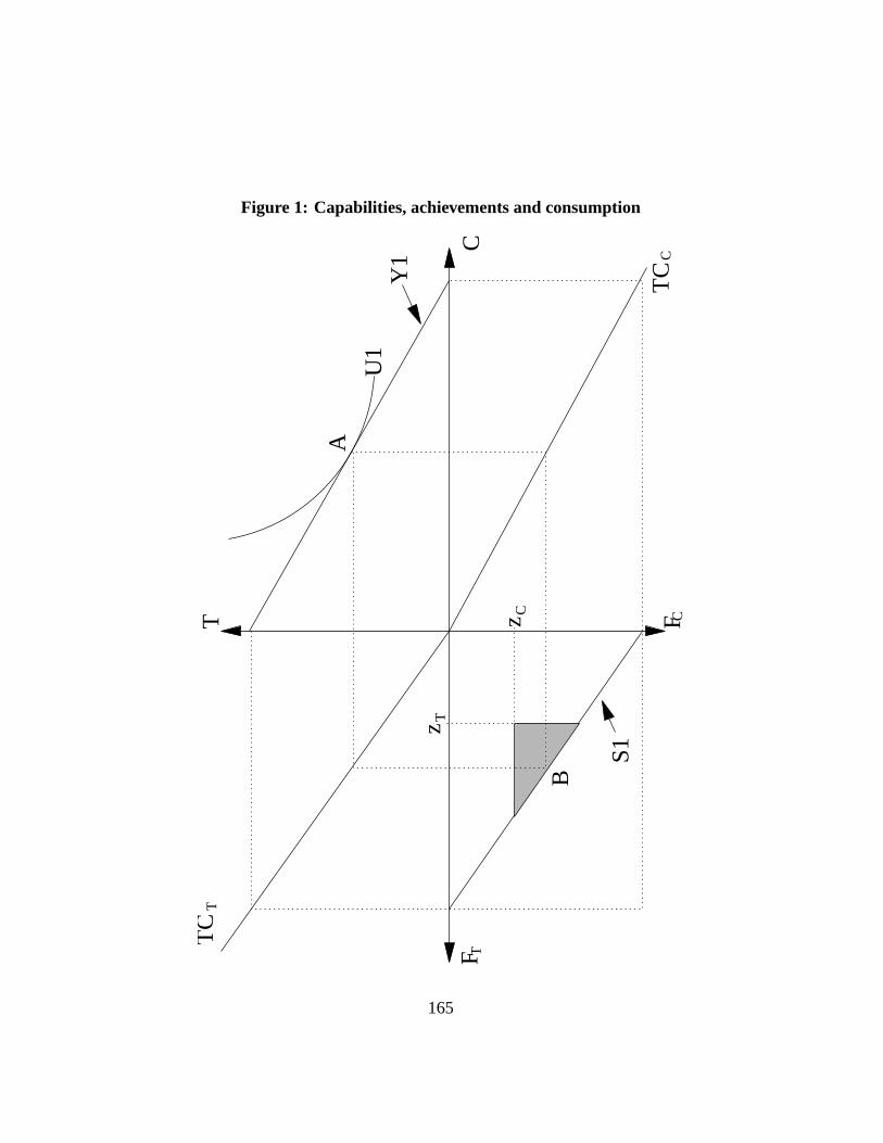
Figure 1: Capabilities, achievements and consumption

CF

F C

T

A

U1

B

z T

z C

TC

TC

T

C

S1

Y1

T

165

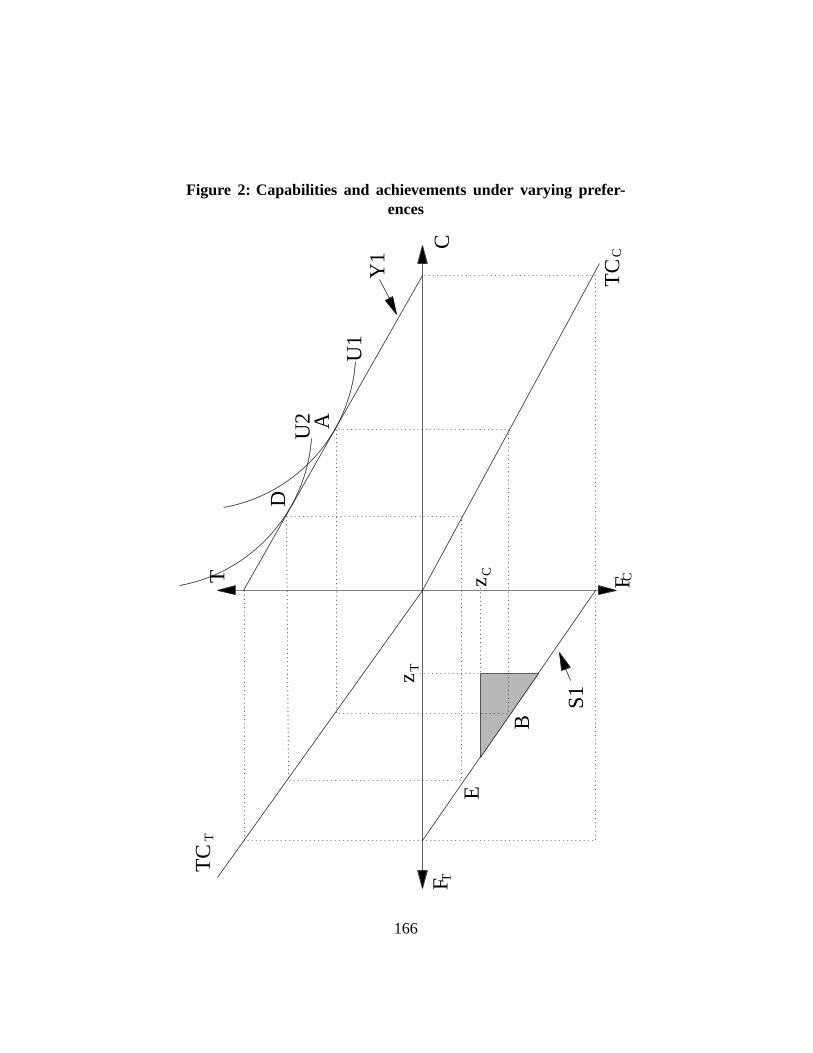
Figure 2: Capabilities and achievements under varying prefer-ences

T

CF

F C

T

A

U1

B

z T

z C

DU

2

E

TC

TC

T

C

S1

Y1

166

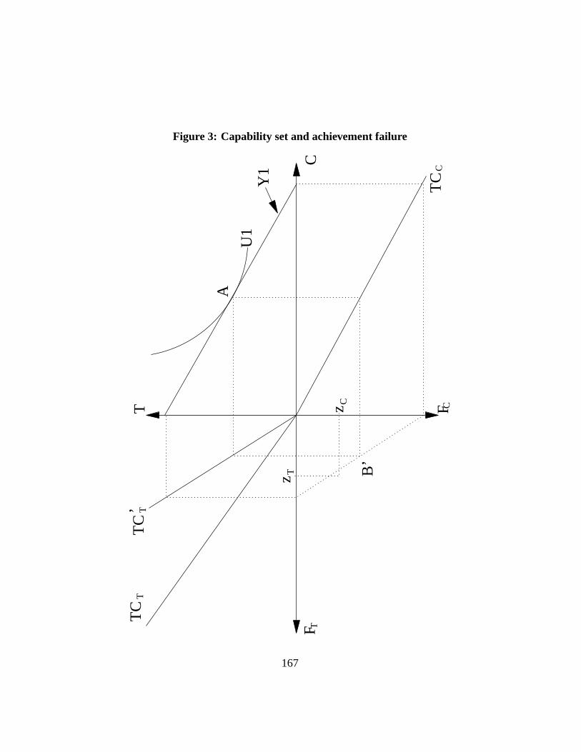
Figure 3: Capability set and achievement failure

CF

F C

T

A

U1

z T

z C

TC

TC

T

C

Y1

TT

CT’

B’

167

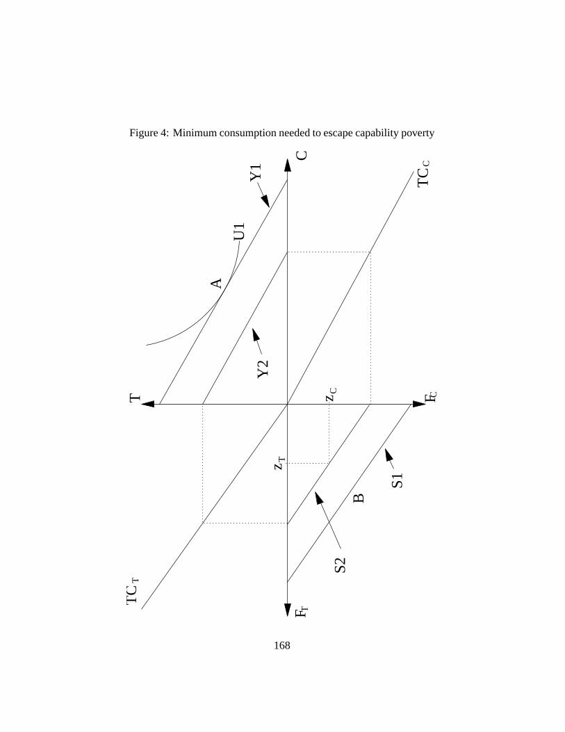
Figure 4:Minimum consumption needed to escape capability poverty

CF

F C

T

A

U1

B

z T

z C

TC

TC

T

C

S1

Y1

T

S2

Y2

168

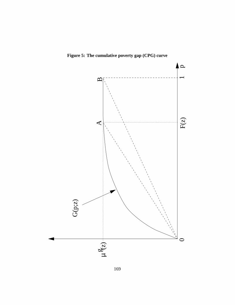
Figure 5: The cumulative poverty gap (CPG) curve

G(p

;z)

µg (z

)

F(z)

p0

1

AB

169

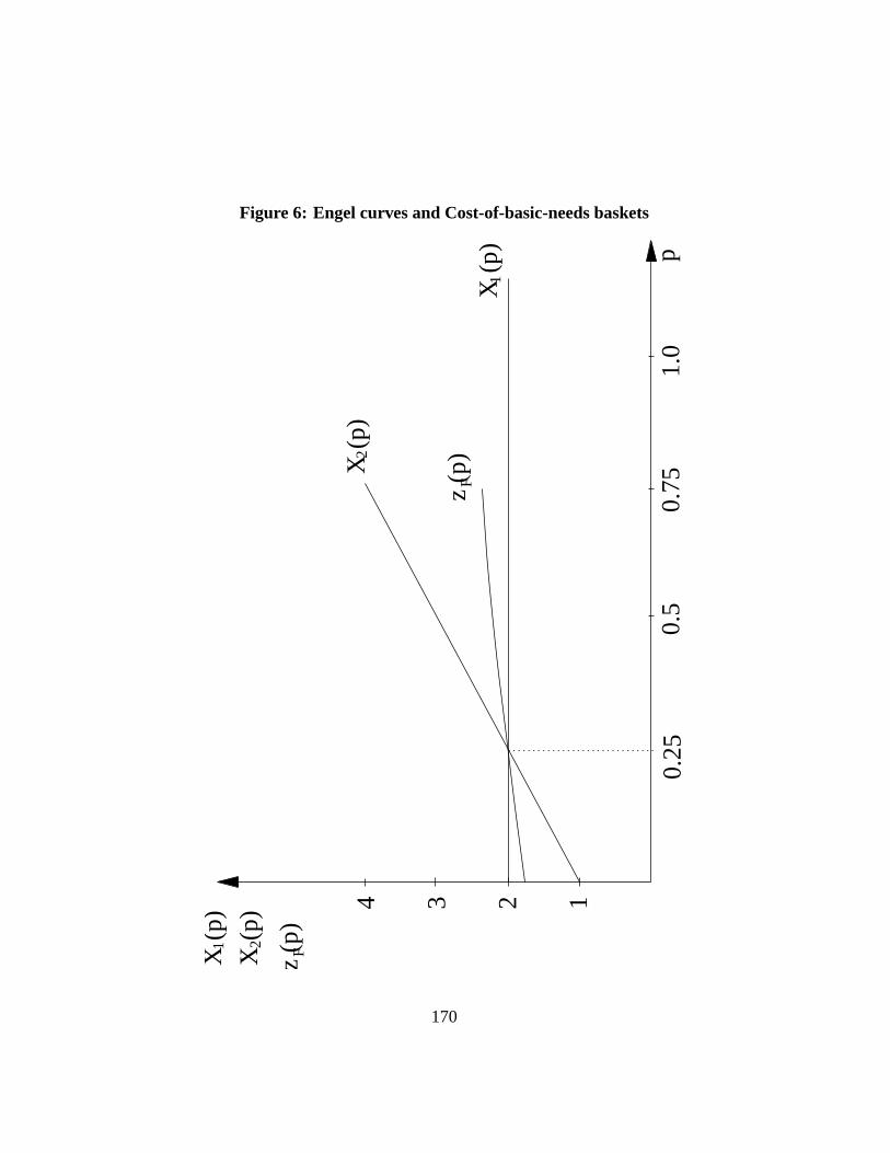
Figure 6: Engel curves and Cost-of-basic-needs baskets

1234

0.25

0.5

0.75

1.0

p

X (

p)1

X (

p)2

X (

p)2

X (

p)1

z (p

)F

z (p

)F

170

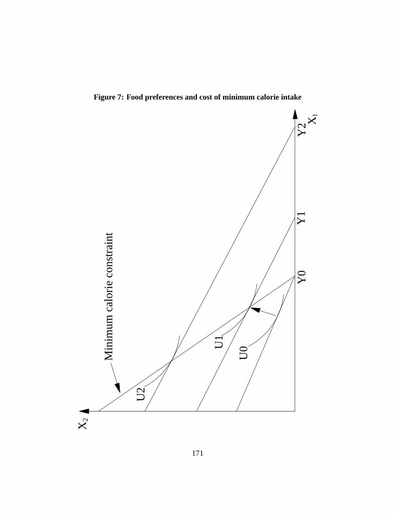
Figure 7: Food preferences and cost of minimum calorie intake

U2

U1

U0

Y0

Y1

Y2 X

1

X2

Min

imum

cal

orie

con

stra

int

171

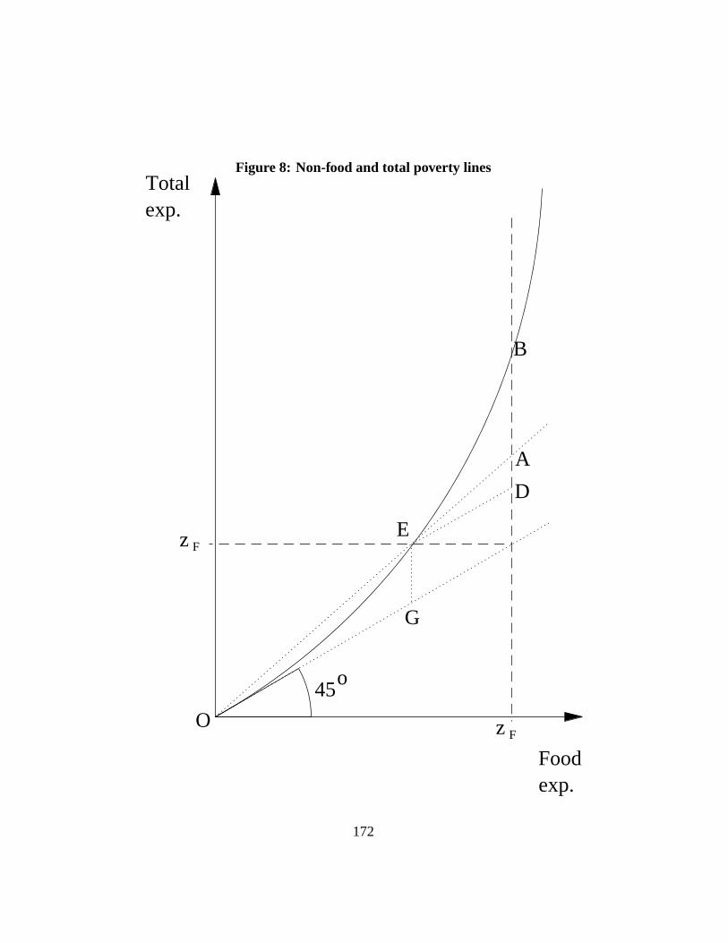
Figure 8: Non-food and total poverty lines

Foodexp.

Totalexp.

z F

45o

z F

A

B

D

E

O

G

172

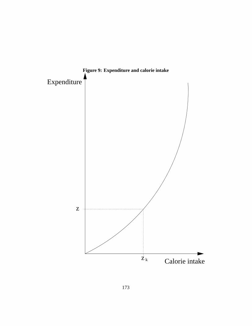
Figure 9: Expenditure and calorie intake

Expenditure

Calorie intakez k

z

173

Figure 10: Subjective poverty linesMinimum subjective income

Inco

me

. ..

.

.

..

.

.

.

.

.

.

.

.

.

.

..

.

.

..

.

..

.

..

z*

z*

a

b

45o

174

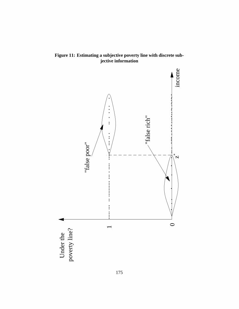
Figure 11: Estimating a subjective poverty line with discrete sub-jective information

Und

er th

epo

vert

y lin

e?

..

..

..

..

..

..

..

....

.. ..

..

..

..

...

..

1 0in

com

e

.....

... .

. ....

......

... .

....

... .

. ..

. .. .

.

. .

. . .

.

z*

"fal

se p

oor" "f

alse

ric

h"

175

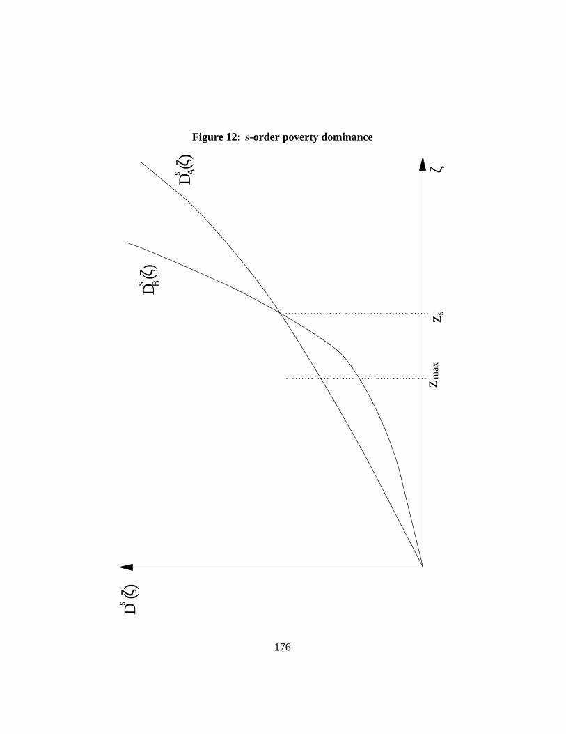
Figure 12: s-order poverty dominanceD

( )

sζ

ζ

D (

)s

ζ

D (

)s

ζA

B

z max

z s

176

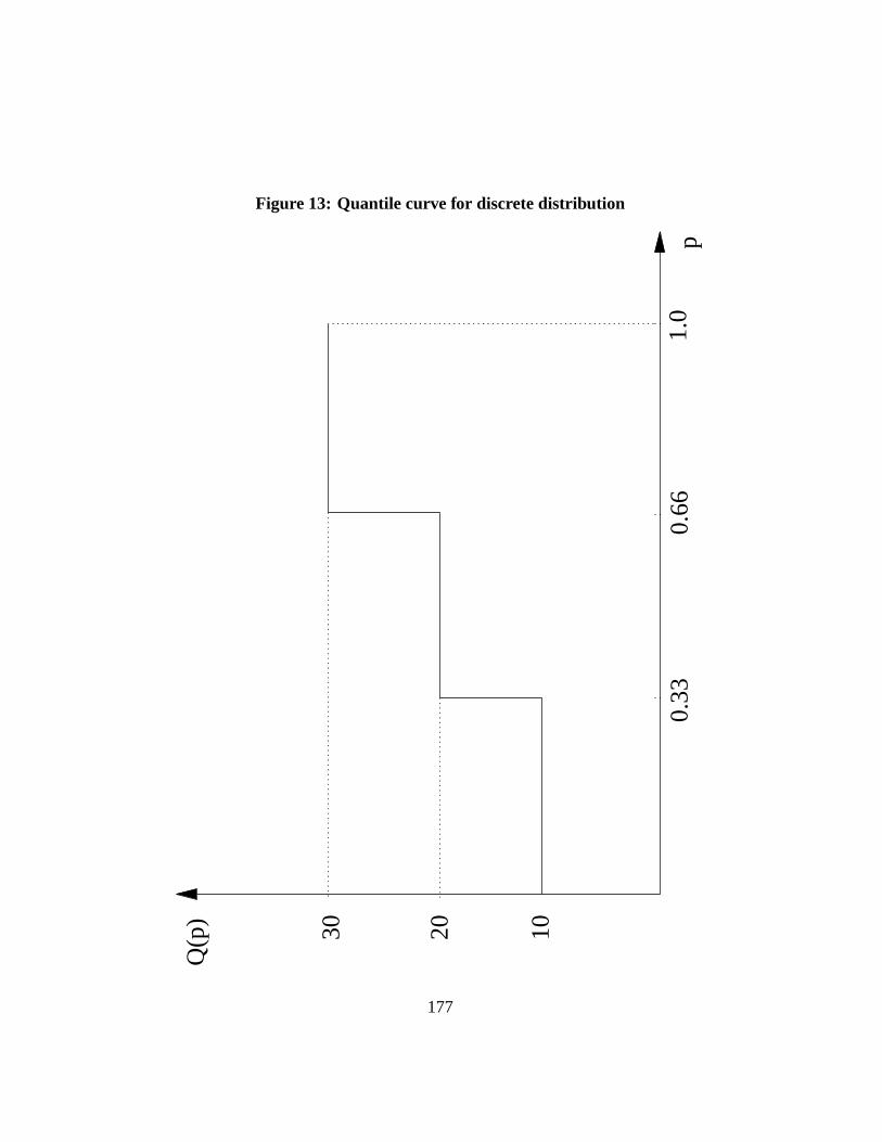
Figure 13: Quantile curve for discrete distributionQ

(p)

p0.

330.

661.

0

102030

177

Figure 14: Quantile curve for continuous distributionQ(p)

y

pF(y)

ymax

1

µ

Q(p)

178

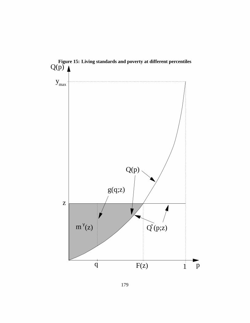
Figure 15: Living standards and poverty at different percentilesQ(p)

p1

ymax

q

g(q;z)

m γ(z)

z

Q (p;z)*

Q(p)

F(z)

179

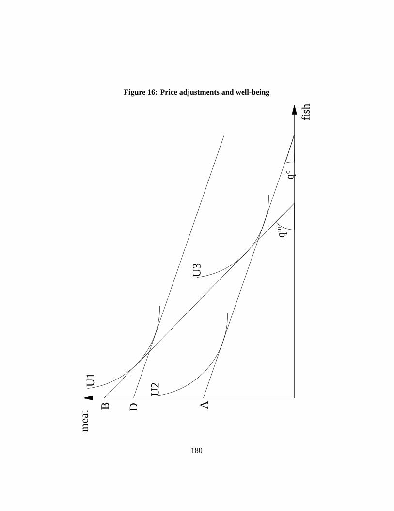
Figure 16: Price adjustments and well-beingm

eat

fish

U1

U3

U2

AB

qm

qc

D

180

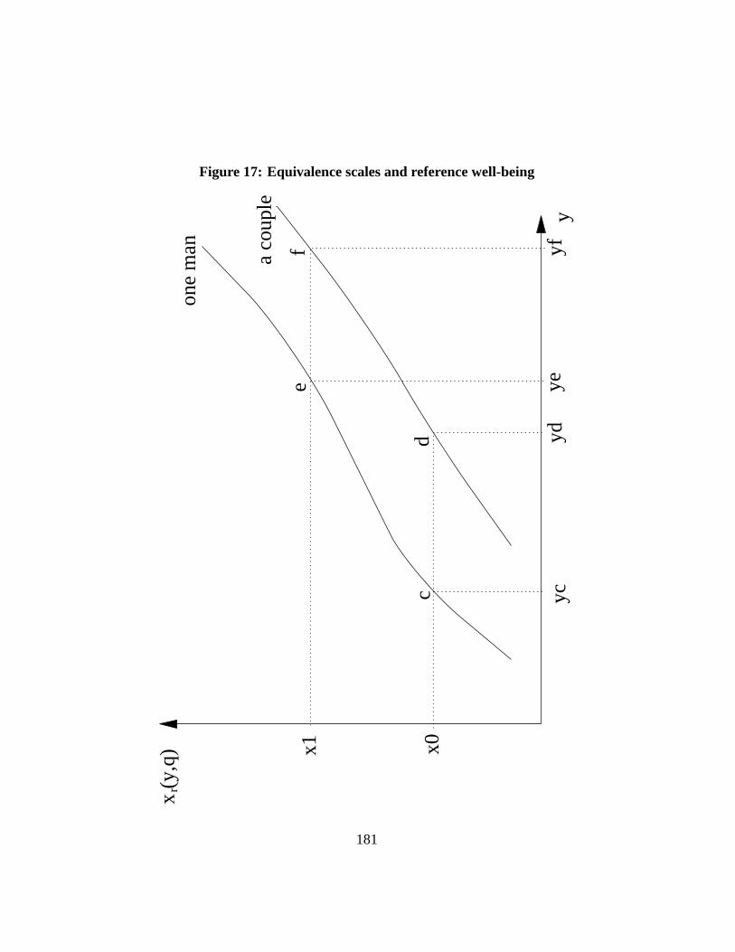
Figure 17: Equivalence scales and reference well-beingx

(y,q

)

y

r

ycyd

yeyf

cd

ef

x0x1

one

man a co

uple

181

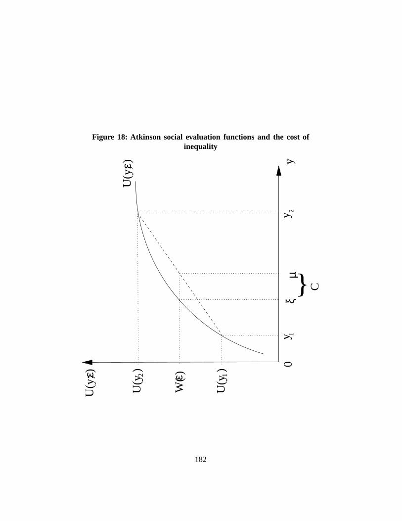
Figure 18: Atkinson social evaluation functions and the cost ofinequality

0y

ξµ

y1

2

C

U(y

; )ε

W(

)ε

y

U(y

; )ε

U(y

) 2

U(y

) 1

182

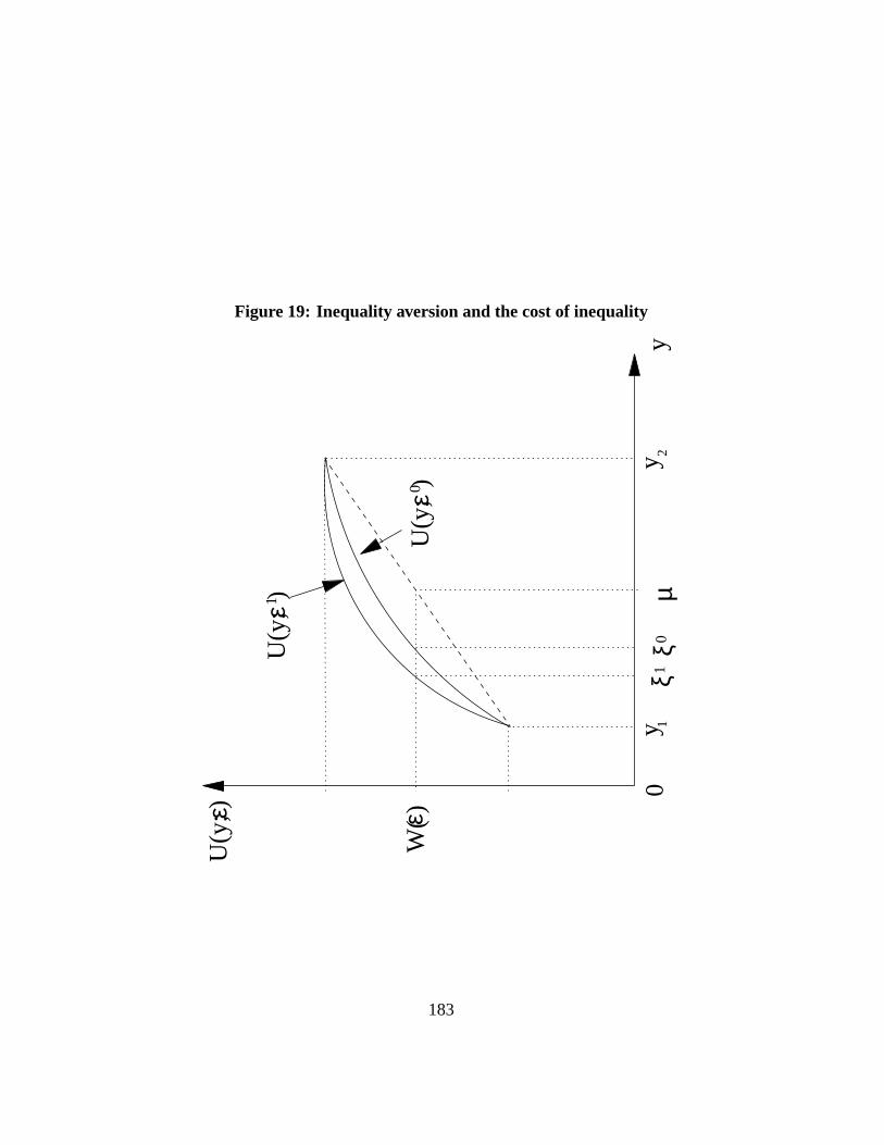
Figure 19: Inequality aversion and the cost of inequality

0y

ξµ

y1

2

U(y

; )

εW

( )ε

y

U(y

; )ε

0

U(y

; )

ε1

0ξ1

183

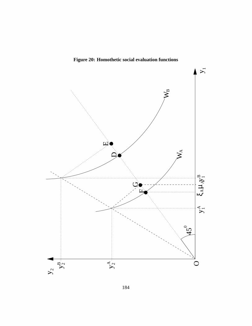
Figure 20: Homothetic social evaluation functions

y 2

y 1

450

WA

WB

y 2 y 2B A

y 1y 1

AB

ξ Aµ

AGF

ED

O

184

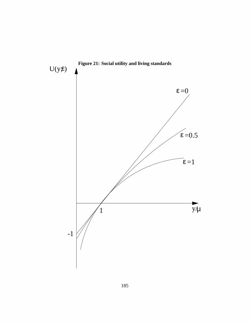
Figure 21: Social utility and living standardsU(y; )ε

y/µ

ε =0.5

ε =0

ε =1

1

-1

185

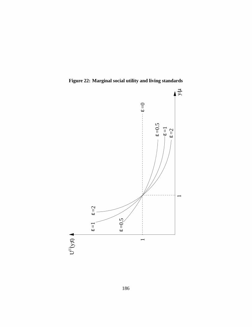
Figure 22: Marginal social utility and living standards

U (

y; )

(1)

ε 1

y/µ

1

ε =0.

5

ε =0

ε =1

ε =2

ε =1

ε =2

ε =0.

5

186

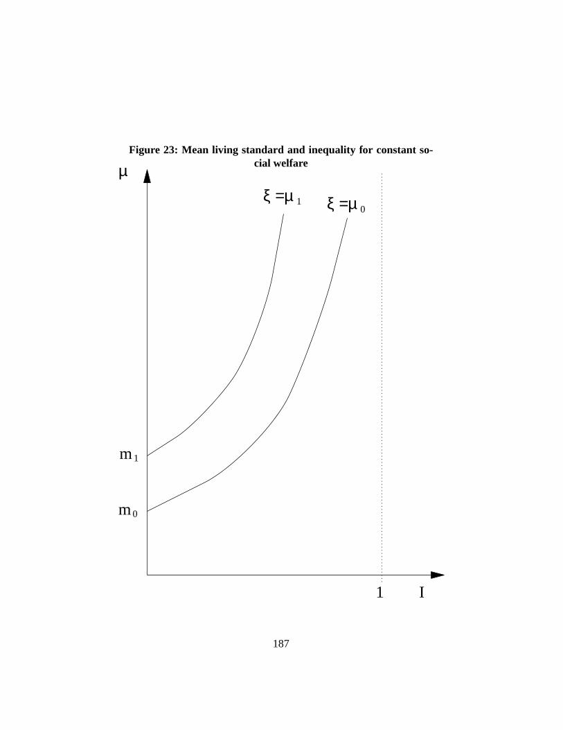
Figure 23: Mean living standard and inequality for constant so-cial welfareµ

I1

m 0

m 1

ξ =µ 1 ξ =µ 0

187

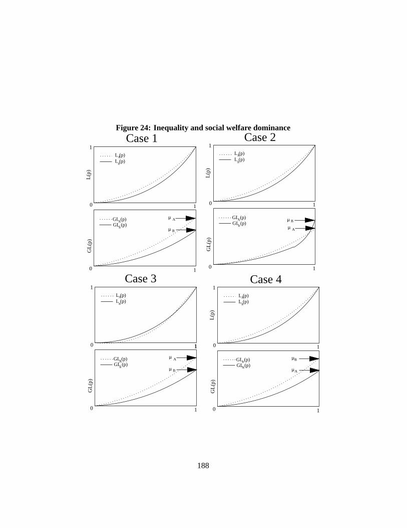
Figure 24: Inequality and social welfare dominance

0

0

1

1

L(p

)G

L(p

)

1

µ

µ

A

B

L (p)L (p)

A

B

A

B

GL (p)GL (p)

0

0

1

1

L(p

)G

L(p

)

1

µ

µ

A

B

L (p)L (p)

A

B

A

B

GL (p)GL (p)

0

1

1

GL

(p)

µ

µ

A

B

A

B

GL (p)GL (p)

0

0

1

1

L(p

)G

L(p

)

1

µ

µA

B

L (p)L (p)

A

B

A

BGL (p)GL (p)

Case 2

Case 3 Case 4

0 1

1

L (p)L (p)

A

B

Case 1

188

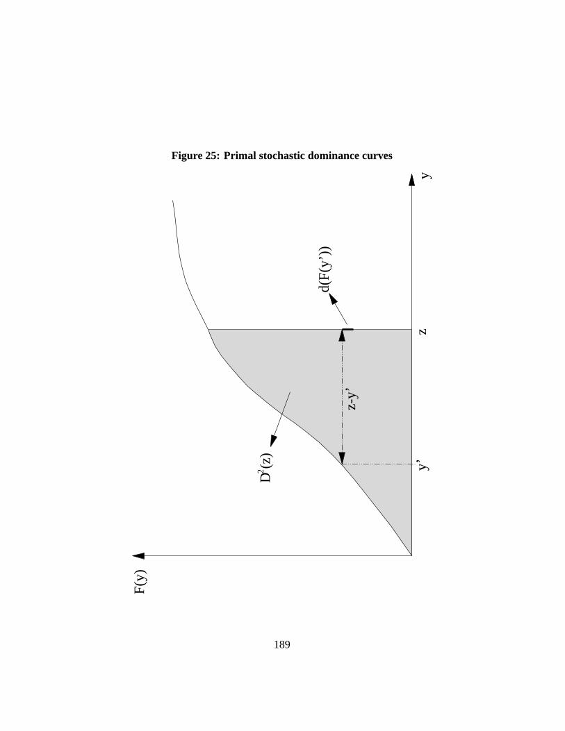
Figure 25: Primal stochastic dominance curvesF(

y)

yz

D (

z)2 y’

z-y’

d(F(

y’))

189

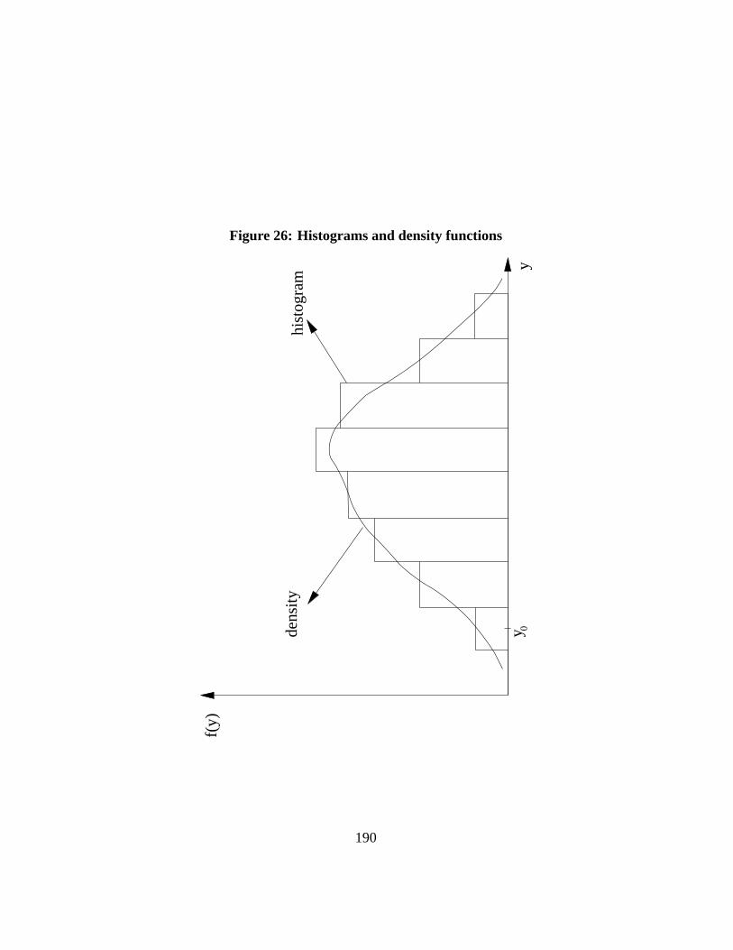
Figure 26: Histograms and density functions

hist

ogra

mde

nsity

f(y)

yy 0

190

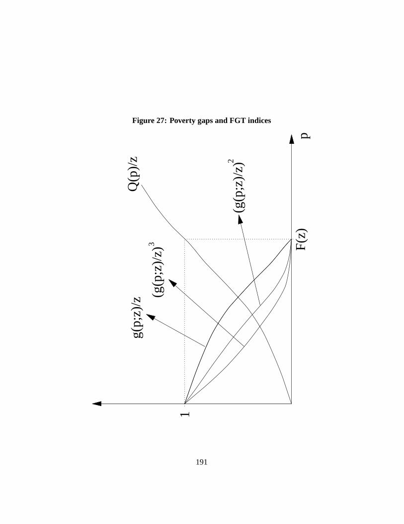
Figure 27: Poverty gaps and FGT indices

pF(

z)

1

Q(p

)/z

g(p;

z)/z

(g(p

;z)/

z)2

(g(p

;z)/

z)3

191

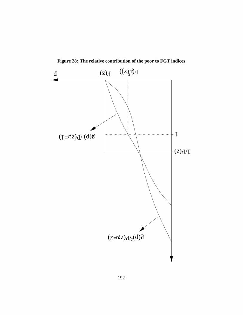
Figure 28: The relative contribution of the poor to FGT indices

p F(z)

1

1/F(z)

g(p) /P(z; =2)2α

g(p) /P(z; =1) α

F( (z)) µg

192

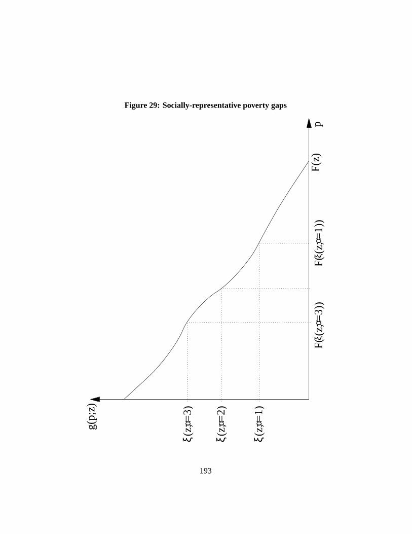
Figure 29: Socially-representative poverty gaps

g(p;

z)

p

ξ(z;

=1)

α

F(z)

ξ(z;

=2)

α

ξ(z;

=3)

α

ξF(

(z;

=3)

)α

ξF(

(z;

=1)

)α

193

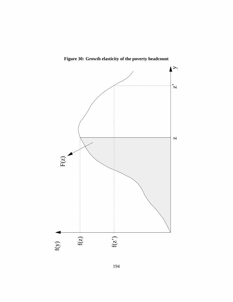
Figure 30: Growth elasticity of the poverty headcountf(

y)F(

z)

zy

f(z)

z’

f(z’

)

194

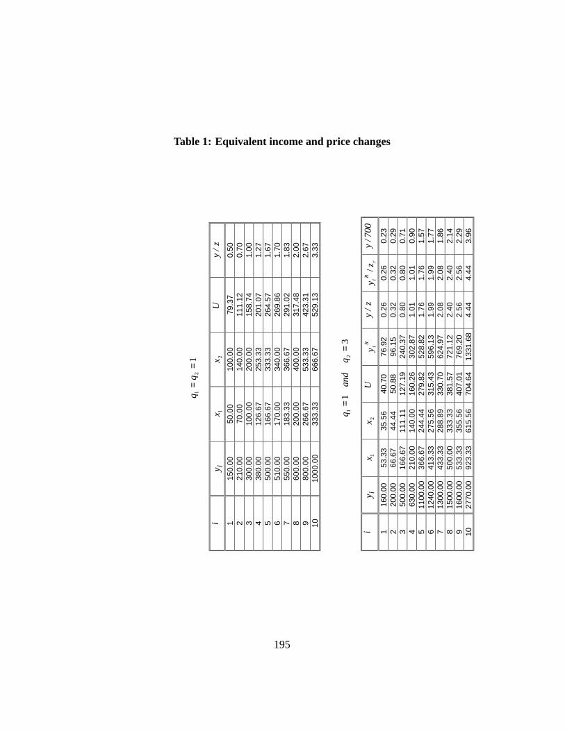
Table 1: Equivalent income and price changes

12

1=

=q

q

i iy

1x

2x

U

z/

y

1 15

0.00

50

.00

100.

00

79.3

7 0.

50

2 21

0.00

70

.00

140.

00

111.

12

0.70

3

300.

00

100.

00

200.

00

158.

74

1.00

4

380.

00

126.

67

253.

33

201.

07

1.27

5

500.

00

166.

67

333.

33

264.

57

1.67

6

510.

00

170.

00

340.

00

269.

86

1.70

7

550.

00

183.

33

366.

67

291.

02

1.83

8

600.

00

200.

00

400.

00

317.

48

2.00

9

800.

00

266.

67

533.

33

423.

31

2.67

10

10

00.0

0 33

3.33

66

6.67

52

9.13

3.

33

31

21

==

qan

dq

i iy

1x

2x

U

R iy

z/

y

rR i

zy

/

700

/y

1 16

0.00

53

.33

35.5

6 40

.70

76.9

2 0.

26

0.26

0.

23

2 20

0.00

66

.67

44.4

4 50

.88

96.1

5 0.

32

0.32

0.

29

3 50

0.00

16

6.67

11

1.11

12

7.19

24

0.37

0.

80

0.80

0.

71

4 63

0.00

21

0.00

14

0.00

16

0.26

30

2.87

1.

01

1.01

0.

90

5 11

00.0

0 36

6.67

24

4.44

27

9.82

52

8.82

1.

76

1.76

1.

57

6 12

40.0

0 41

3.33

27

5.56

31

5.43

59

6.13

1.

99

1.99

1.

77

7 13

00.0

0 43

3.33

28

8.89

33

0.70

62

4.97

2.

08

2.08

1.

86

8 15

00.0

0 50

0.00

33

3.33

38

1.57

72

1.12

2.

40

2.40

2.

14

9 16

00.0

0 53

3.33

35

5.56

40

7.01

76

9.20

2.

56

2.56

2.

29

10

2770

.00

923.

33

615.

56

704.

64

1331

.68

4.44

4.

44

3.96

195

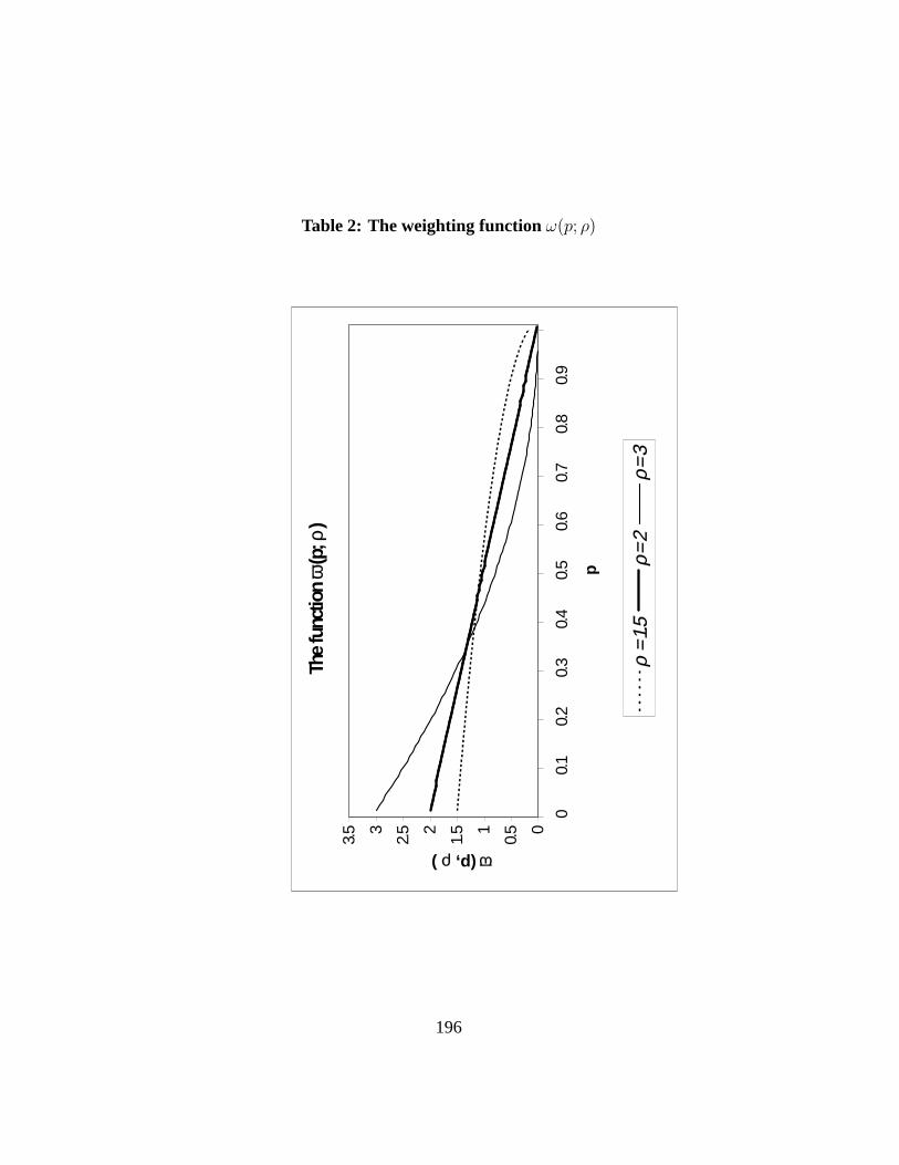
Table 2: The weighting function ω(p; ρ)

The

func

tion

ωω (p

; ρρ )

0

0.51

1.52

2.53

3.5

00.

10.

20.

30.

40.

50.

60.

70.

80.

9

p

ωω (p, ρρ )

ρ =

ρ = 11

..55ρ =

ρ =

22ρ =

ρ =

33

196

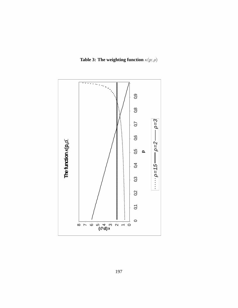
Table 3: The weighting function κ(p; ρ)

The

func

tion

κκ((p ,,

ρρ))

012345678

00,

10,

20,

30,

40,

50,

60,

70,

80,

9

p

κκ(p,ρρ)

ρ =

ρ = 11..

55ρ =

ρ =

22ρ =

ρ =

33

197

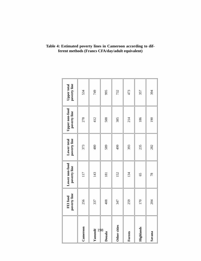
Table 4: Estimated poverty lines in Cameroon according to dif-ferent methods (Francs CFA/day/adult equivalent)

F

EI

food

po

vert

y lin

e

Low

er n

on-f

ood

pove

rty

line

L

ower

tot

al

pove

rty

line

Upp

er n

on-f

ood

pove

rty

line

Upp

er t

otal

po

vert

y lin

e

Cam

eroo

n 25

6 11

7 37

3 27

8 53

4

Yao

undé

33

7 14

3 48

0 41

2 74

9

Dou

ala

408

181

589

588

995

Oth

er c

itie

s 34

7 15

2 49

9 38

5 73

2

For

ests

25

9 13

4 39

3 21

4 47

3

Hig

hlan

ds

170

65

235

186

357

Sava

na

204

78

282

190

394

198

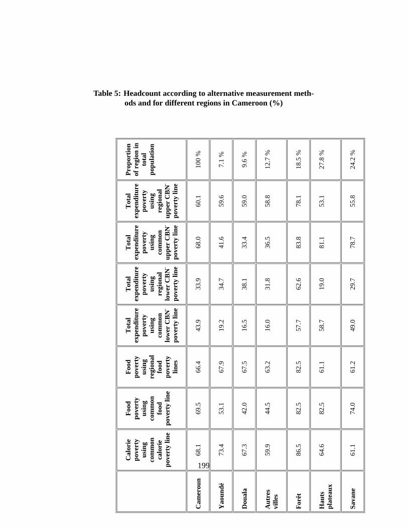
Table 5: Headcount according to alternative measurement meth-ods and for different regions in Cameroon (%)

C

alor

ie

pove

rty

usin

g co

mm

on

calo

rie

pove

rty

line

Foo

d po

vert

y us

ing

com

mon

fo

od

pove

rty

line

Foo

d po

vert

y us

ing

regi

onal

fo

od

pove

rty

lines

Tot

al

expe

ndit

ure

pove

rty

usin

g co

mm

on

low

er C

BN

-

pove

rty

line

Tot

al

expe

ndit

ure

pove

rty

usin

g re

gion

al

low

er C

BN

-

pove

rty

line

Tot

al

expe

ndit

ure

pove

rty

usin

g co

mm

on

uppe

r C

BN

-

pove

rty

line

Tot

al

expe

ndit

ure

pove

rty

usin

g re

gion

al

uppe

r C

BN

-

pove

rty

line

Pro

port

ion

of r

egio

n in

to

tal

popu

lati

on

Cam

erou

n 68

.1

68.1

69

.5

66.4

43

.9

33.9

68

.0

60.1

10

0 %

Yao

undé

73

.4

73.4

53

.1

67.9

19

.2

34.7

41

.6

59.6

7.

1 %

Dou

ala

67.3

67

.3

42.0

67

.5

16.5

38

.1

33.4

59

.0

9.6

%

Aut

res

vill

es

59.9

59

.9

44.5

63

.2

16.0

31

.8

36.5

58

.8

12.7

%

For

êt

86.5

86

.5

82.5

82

.5

57.7

62

.6

83.8

78

.1

18.5

%

Hau

ts

plat

eaux

64

.6

64.6

82

.5

61.1

58

.7

19.0

81

.1

53.1

27

.8 %

Sava

ne

61.1

61

.1

74.0

61

.2

49.0

29

.7

78.7

55

.8

24.2

%

199

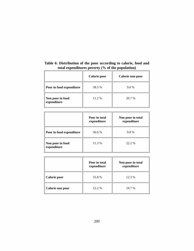
Table 6: Distribution of the poor according to calorie, food andtotal expenditures poverty (% of the population)

Calorie poor Calorie non-poor

Poor in food expenditure 58.5 % 9.6 %

Non poor in food expenditure

11.2 % 20.7 %

Poor in total expenditure

Non poor in total expenditure

Poor in food expenditure 56.6 % 9.8 %

Non poor in food expenditure

11.3 % 22.2 %

Poor in total expenditure

Non poor in total expenditure

Calorie poor 55.8 % 12.3 %

Calorie non poor 12.2 % 19.7 %

200