Embed Size (px)
Citation preview

Poverty Accounting
A fractional response approach to poverty decomposition∗
Richard Bluhm† Denis de Crombrugghe‡ Adam Szirmai§
August 2016
Working Paper
Abstract
This paper proposes a new empirical framework for poverty accounting. Using
a large collection of household surveys from 124 countries, we estimate income and
inequality (semi-)elasticities of poverty for the $2 and $1.25 a day poverty lines as
well as their contributions to poverty alleviation. We show that initial inequality
is a strong moderator of the impact of growth and there has been a shift towards
more pro-poor growth around the turn of the millennium. We project poverty rates
until 2030 and show that an end of extreme poverty within a generation is unlikely.
Keywords: poverty, inequality, income growth, fractional response models
JEL Classification: I32, C25, O10, O15
∗This paper and previous versions have been presented at the World Bank, ECINEQ, Agence Francaisede Developpement, Center for Global Development, IARIW, UGottingen, OECD, a workshop on paneldata methods (UMainz) and several workshops in Paris and Maastricht. We have greatly benefitedfrom discussions with the participants. In particular, we would like to thank Florent Bresson, LaurenceChandy, Martin Gassebner, Gary Hoover, Pierre Mohnen, Charles Kenny, Stephan Klasen, MelanieKrause, Nicolas Meisel, Christophe Muller, D.S. Prasada Rao, Thomas Roca, Susanne Steiner, KajThomsson, Bart Verspagen and Jeffrey Wooldridge. We gratefully acknowledge financial support fromthe Agence Francaise de Developpement (AFD). All remaining errors are unfortunately ours.†Corresponding author. Leibniz University Hannover, Institute of Macroeconomics, and UNU-
MERIT, Maastricht University; e-mail: [email protected]‡Maastricht University; e-mail: [email protected]§UNU-MERIT, Maastricht University; e-mail: [email protected]
1
1 Introduction
The capacity of economic growth to eradicate poverty is at the heart of ongoing debates
over inclusive growth and equitable development. Okun’s famous equality-efficiency
trade-off dominated the discussion until the turn of the 21st century and often meant
that equity was sacrificed in favor of ‘efficiency’. It has since been replaced by a renewed
focus on ‘pro-poor growth’ (World Bank, 2005) and ‘shared prosperity’ (World Bank,
2015). The shift in the policy discussion is underscored by an increasingly large empirical
literature that analyzes the impact of changes in incomes and inequality on poverty, or
their respective contributions towards poverty reduction (see e.g. Ravallion and Chen,
1997; Dollar and Kraay, 2002; Besley and Burgess, 2003; Kraay, 2006; Kalwij and
Verschoor, 2007; Dollar et al., 2016). Collectively, these studies established not only
that income growth is crucial to achieving sustained decreases in poverty, but also that
the benefits of income growth strongly depend on initial levels of income and inequality.
In fact, this dependence arises mechanically, since poverty is functionally linked to average
incomes and inequality (Datt and Ravallion, 1992; Kakwani, 1993; Bourguignon, 2003).
In this paper we present a new unified framework for a set of empirical exercises we
collectively refer to as ‘poverty accounting’. Analogous with growth and development
accounting, poverty accounting is the decomposition of (changes in or levels of) poverty
into its proximate sources. It is concerned with answering several important and related
questions, such as: What is the impact of a one percent change in income growth or in
inequality on poverty rates? How much of the historical variation in poverty is due to
economic growth? How much is due to redistribution? Just as in the decomposition of
growth, there is some uncertainty concerning the correct functional form of the underlying
relationship. Yet, unlike the case of economic growth, there is no ambiguity about the
fact that, at the proximate level, the poverty rate in any country or region is entirely
determined by the average income level and the income distribution.
The key insight we build on in this paper is that the poverty headcount ratio is
a fraction. This fact alone allows us to derive a very natural model of the expected
poverty rate, E[H], given a fixed (absolute) poverty line. The model incorporates two
crucial features: first, E[H] is bounded on the unit interval; and second, E[H] converges
to unity (zero) if mean income becomes arbitrarily small (large) relative to the poverty
line. It is immediately clear that elasticities or semi-elasticities of poverty with respect
to income or inequality must be non-linear. So far, the literature has tried to address
this inherent non-linearity within log-linear models, leading to specifications which are
poor approximations and tend to produce unstable or implausible estimates for anything
but overall mean effects. To policy makers though, cross-country averages of elasticities
are of limited interest. Even within countries, evidence points towards substantially
different impacts of growth on poverty across regions or ethnic groups (Aaron, 1967;
2
Hoover et al., 2008). In other words, when it comes to models of poverty rates, one of
the main virtues of linear regression – its ability to consistently identify average effects –
leads to disappointingly few insights.
We propose a fractional response approach to deal with the inherent non-linearity
of the poverty decomposition (Papke and Wooldridge, 1996, 2008). This approach
dispenses with the constant or linear elasticities assumed by much of the empirical cross-
country literature. It allows us to (i) estimate elasticities and semi-elasticities of poverty
with respect to income or inequality with great precision over the entire range of the
observed data, (ii) recover the conditional expectation of the poverty headcount ratio,
and (iii) estimate the counterfactual quantities needed for computing the contribution
of either factor to overall poverty reduction. Nonetheless, estimation of these quantities
based on household surveys typically entails a number of problems. Hence, we present
extensions of the fractional response framework that deal with unobserved heterogeneity
due to persistent measurement differences between surveys, endogeneity due to time-
varying measurement errors in incomes, and unbalanced panel data due to infrequently
undertaken surveys. While our application focuses on the cross-country distribution of
poverty rates, our framework can also be used to decompose poverty rates across regions
of any country with a fixed poverty line (e.g. the United States, India or China).
A powerful side effect of focusing directly on E[H] is that we can estimate the impact
of changes in the average level or the distribution of income, use in-sample predictions to
estimate their respective historical contributions, and engage in out-of-sample forecasting,
all within a single framework. Note that ‘impact’ refers to the response of poverty to
shifts in its proximate determinants, whereas ‘contribution’ refers to what part of the
historically observed variation in poverty is due to each factor. As a consequence of
Jensen’s inequality, log-linearized models of the poverty headcount ratio (whether in levels
or in differences) cannot recover the conditional expectation of the poverty rate without
imposing strong or implausible assumptions. As a result, impacts and contributions of
the proximate sources of poverty are usually not estimated within the same model. Log-
linearized models also imply the loss of all poverty spells starting or ending with a poverty
rate of zero and extreme sensitivity to small variations in poverty rates near zero.1 Our
approach avoids these shortcomings.
We apply this empirical framework to a new data set of 809 nationally representative
surveys covering 124 countries in the period 1981–2010. In their most basic form, the
data only contain three variables per country-survey-year: the poverty headcount ratio
at a fixed international poverty line, average income, and a measure of dispersion such as
the Gini coefficient. This is the typical data faced by a researcher who lacks a worldwide
1See Santos Silva and Tenreyro (2006) on the pitfalls of log-linear estimation of gravity models. Heretoo, the presence of heteroskedasticity implies that parameter estimates from log-linearized models arenot just inefficient but are also likely to be biased.
3
household (panel) survey. At the micro level, it would be possible to directly estimate
the Lorenz curve, take the corresponding derivatives for the elasticities, and calculate
the relevant counterfactual quantities to estimate the contributions (see e.g. Datt and
Ravallion, 1992). Hence, a viable alternative to our method is to apply the micro-level
approach to all countries by creating synthetic data as in Kraay (2006), but Lorenz curve
estimation based on grouped data has its own problems (see e.g. Chotikapanich et al.,
2007; Bresson, 2009; Krause, 2014, on the characteristics of the implied density functions).
Our approach, in contrast, can closely approximate the shape of the Lorenz curve near
the poverty line using only very limited information.
Our main findings are as follows. Regarding the average impact of growth or
distributional change on poverty, we find that a one percent increase in mean income
or consumption expenditures reduces the proportion of people living below the poverty
line by about two percentage points, while a similar increase in inequality raises the
poverty rate by one and a half percentage points. Both of these average effects are at the
lower end of those typically found in the literature. The upshot is, our approach provides
differentiated and considerably more precise regional and temporal estimates, often at
odds with earlier studies. For example, we find universally higher income elasticities
in Latin America or Eastern Europe and Central Asia but lower income elasticities in
South Asia or Sub-Saharan Africa than reported earlier (Kalwij and Verschoor, 2007).
Since elasticities are concepts of relative change they may give the misleading impression
that richer countries (with fewer poor) are becoming ever better at reducing poverty,
even though the underlying absolute changes are very small. Hence, we also focus on
semi-elasticities which measure the response of poverty in terms of the percentage point
change in the population that is poor (see also Klasen and Misselhorn, 2008). Not only
are these quantities much less sensitive to small variations in the data, they are much
more relevant for policy makers who presumably think about poverty reduction in terms
of people, not relative changes in poverty rates. The choice of elasticities versus semi-
elasticities also matters conceptually. We show that a proportional decomposition (which
implicitly uses elasticities) understates the contribution of growth to poverty reduction
in poorer countries and overstates it in richer countries.2
Regarding historical contributions, we provide new evidence that there has been a shift
in the poverty reducing pattern of growth around the turn of the millennium. Before 2000
about 90% of poverty reduction was due to income growth, and inequality tended to rise
with higher growth rates. Since 2000, changes in inequality are responsible for almost a
third of all poverty reduction. Recent growth has also been substantially more pro-poor,
both in the absolute sense of reducing poverty more often than not, and in the relative
sense of coinciding with reductions in inequality more often. The results are similar at
2See Cuaresma et al. (2016), who highlight that semi-elasticity specifications resolve the puzzlepresented by Ravallion (2012) and recover cross-country convergence in poverty rates.
4
the $2 a day and $1.25 a day poverty lines. This is good news for the prospects of global
poverty reduction. Many countries in Sub-Saharan Africa are in a situation where the
bulk of the distribution is still below the extreme poverty line. As they grow richer,
reductions in inequality could contribute considerably more to poverty reduction than
they have in the past because inequality semi-elasticities are bound to increase.
Finally, we present projections of the poverty headcount ratio for the $2 a day and
$1.25 a day poverty lines until 2030 in 2005 PPPs. We find that absolute poverty in
Sub-Saharan Africa and, as a not too distant second, South Asia remains the primary
development challenge of the twenty-first century. Although economic growth has
accelerated significantly since 2000, poverty reduction in the developing world outside
China has been slow. Most of the poverty reduction potential coming from China is now
exhausted. Nevertheless, we show that the $2 a day poverty rate may halve from about
40% in 2010 to below 20% in 2030. This implies another billion people could be lifted
out of poverty in the meantime. The bad news is that the pace of poverty reduction
at $1.25 a day is bound to slow down significantly in the near future. Extreme poverty
barely falls below 8% of the developing world population in the most optimistic scenario.
These results differ from Ravallion (2013), who first proposed the new 3% target, because
population growth tends to be faster and consumption growth slower in countries with
high poverty rates. Our growth scenarios are based on each country’s own growth record,
not the average experience of the entire developing world. None of our scenarios predicts
a poverty rate near 3% once country-specific trends from 2000 to 2010 are used. Hence,
reaching the first of the new sustainable development goals (SDGs) requires both another
acceleration of growth and significant reductions in interpersonal inequality in the poorer
parts of the developing world.
The remainder of this paper is organized as follows. Section 2 reviews how the existing
literature decomposes poverty rates and estimates poverty elasticities. Section 3 explains
our approach and discusses the econometrics of fractional response models. Section 4
briefly outlines the data used in this paper. Section 5 presents the estimation results,
elasticities, contributions, and poverty projections until 2030. Section 6 concludes.
2 Poverty decompositions and elasticities
With micro-level data it is straightforward to decompose changes in poverty into changes
in the average level and the distribution of income (Datt and Ravallion, 1992; Kakwani,
1993). A key problem for cross-country studies of poverty is that we typically do not have
access to micro-data of incomes or consumption expenditures for all countries but have
to estimate poverty using only grouped data.3 To overcome this limitation, Bourguignon
3There have been some attempts either to collect all the available primary data or to repair gapsin survey coverage with the help of national accounts. Milanovic (2002) compiles a global data set of
5
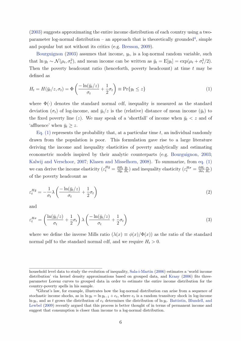
(2003) suggests approximating the entire income distribution of each country using a two-
parameter log-normal distribution – an approach that is theoretically grounded4, simple
and popular but not without its critics (e.g. Bresson, 2009).
Bourguignon (2003) assumes that income, yt, is a log-normal random variable, such
that ln yt ∼ N (µt, σ2t ), and mean income can be written as yt = E[yt] = exp(µt + σ2
t /2).
Then the poverty headcount ratio (henceforth, poverty headcount) at time t may be
defined as
Ht = H(yt/z, σt) = Φ
(− ln(yt/z)
σt+
1
2σt
)≡ Pr{yt ≤ z} (1)
where Φ(·) denotes the standard normal cdf, inequality is measured as the standard
deviation (σt) of log-income, and yt/z is the (relative) distance of mean income (yt) to
the fixed poverty line (z). We may speak of a ‘shortfall’ of income when yt < z and of
‘affluence’ when yt ≥ z.
Eq. (1) represents the probability that, at a particular time t, an individual randomly
drawn from the population is poor. This formulation gave rise to a large literature
deriving the income and inequality elasticities of poverty analytically and estimating
econometric models inspired by their analytic counterparts (e.g. Bourguignon, 2003;
Kalwij and Verschoor, 2007; Klasen and Misselhorn, 2008). To summarize, from eq. (1)
we can derive the income elasticity (εHyt = ∂Ht
∂yt
ytHt
) and inequality elasticity (εHσt = ∂Ht
∂σtσtHt
)
of the poverty headcount as
εHyt = − 1
σtλ
(− ln(yt/z)
σt+
1
2σt
)(2)
and
εHσt =
(ln(yt/z)
σt+
1
2σt
)λ
(− ln(yt/z)
σt+
1
2σt
)(3)
where we define the inverse Mills ratio (λ(x) ≡ φ(x)/Φ(x)) as the ratio of the standard
normal pdf to the standard normal cdf, and we require Ht > 0.
household level data to study the evolution of inequality, Sala-i-Martin (2006) estimates a ‘world incomedistribution’ via kernel density approximations based on grouped data, and Kraay (2006) fits three-parameter Lorenz curves to grouped data in order to estimate the entire income distribution for thecountry-poverty spells in his sample.
4Gibrat’s law, for example, illustrates how the log-normal distribution can arise from a sequence ofstochastic income shocks, as in ln yt = ln yt−1 + et, where et is a random transitory shock in log-incomeln yt, and as t grows the distribution of et determines the distribution of ln yt. Battistin, Blundell, andLewbel (2009) recently argued that this process is better thought of in terms of permanent income andsuggest that consumption is closer than income to a log-normal distribution.
6
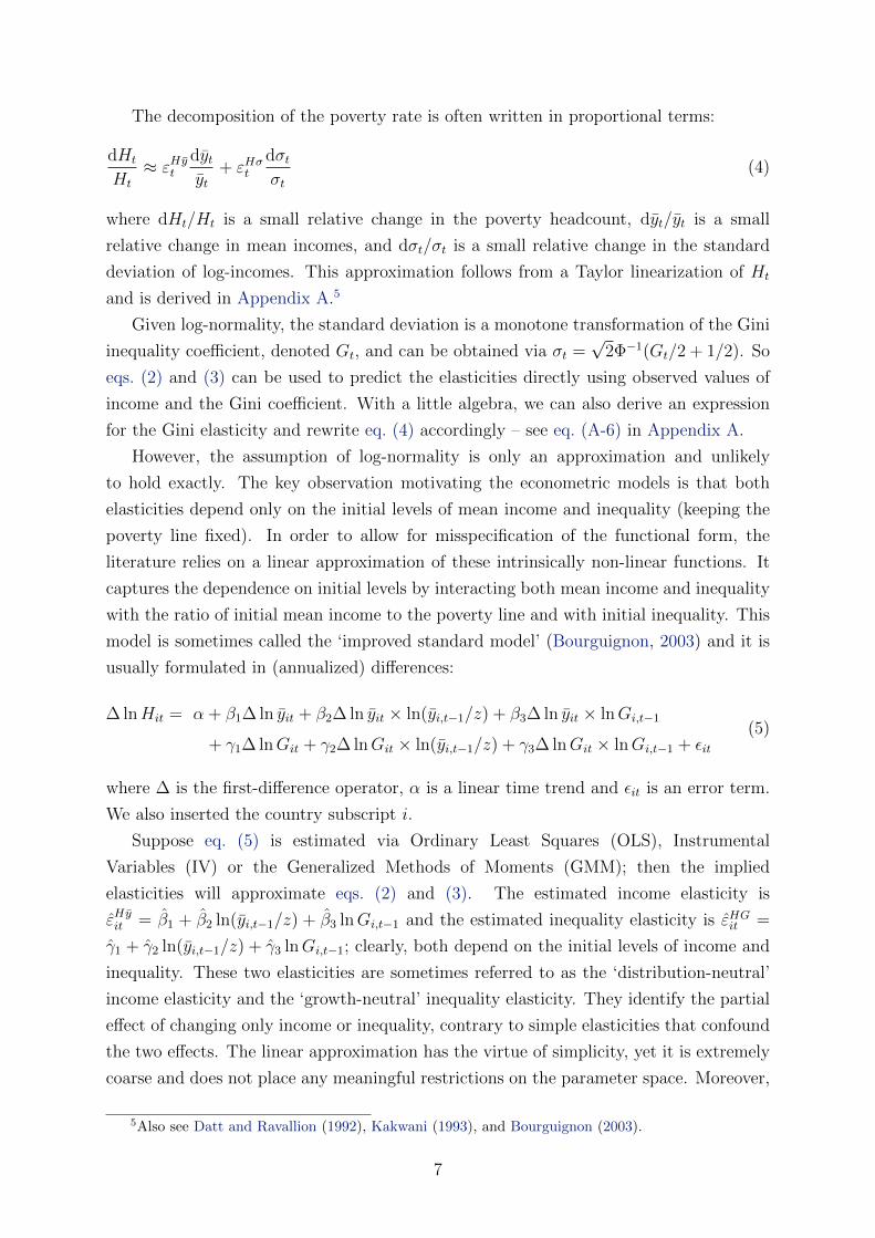
The decomposition of the poverty rate is often written in proportional terms:
dHt
Ht
≈ εHytdytyt
+ εHσtdσtσt
(4)
where dHt/Ht is a small relative change in the poverty headcount, dyt/yt is a small
relative change in mean incomes, and dσt/σt is a small relative change in the standard
deviation of log-incomes. This approximation follows from a Taylor linearization of Ht
and is derived in Appendix A.5
Given log-normality, the standard deviation is a monotone transformation of the Gini
inequality coefficient, denoted Gt, and can be obtained via σt =√
2Φ−1(Gt/2 + 1/2). So
eqs. (2) and (3) can be used to predict the elasticities directly using observed values of
income and the Gini coefficient. With a little algebra, we can also derive an expression
for the Gini elasticity and rewrite eq. (4) accordingly – see eq. (A-6) in Appendix A.
However, the assumption of log-normality is only an approximation and unlikely
to hold exactly. The key observation motivating the econometric models is that both
elasticities depend only on the initial levels of mean income and inequality (keeping the
poverty line fixed). In order to allow for misspecification of the functional form, the
literature relies on a linear approximation of these intrinsically non-linear functions. It
captures the dependence on initial levels by interacting both mean income and inequality
with the ratio of initial mean income to the poverty line and with initial inequality. This
model is sometimes called the ‘improved standard model’ (Bourguignon, 2003) and it is
usually formulated in (annualized) differences:
∆ lnHit = α + β1∆ ln yit + β2∆ ln yit × ln(yi,t−1/z) + β3∆ ln yit × lnGi,t−1
+ γ1∆ lnGit + γ2∆ lnGit × ln(yi,t−1/z) + γ3∆ lnGit × lnGi,t−1 + εit(5)
where ∆ is the first-difference operator, α is a linear time trend and εit is an error term.
We also inserted the country subscript i.
Suppose eq. (5) is estimated via Ordinary Least Squares (OLS), Instrumental
Variables (IV) or the Generalized Methods of Moments (GMM); then the implied
elasticities will approximate eqs. (2) and (3). The estimated income elasticity is
εHyit = β1 + β2 ln(yi,t−1/z) + β3 lnGi,t−1 and the estimated inequality elasticity is εHGit =
γ1 + γ2 ln(yi,t−1/z) + γ3 lnGi,t−1; clearly, both depend on the initial levels of income and
inequality. These two elasticities are sometimes referred to as the ‘distribution-neutral’
income elasticity and the ‘growth-neutral’ inequality elasticity. They identify the partial
effect of changing only income or inequality, contrary to simple elasticities that confound
the two effects. The linear approximation has the virtue of simplicity, yet it is extremely
coarse and does not place any meaningful restrictions on the parameter space. Moreover,
5Also see Datt and Ravallion (1992), Kakwani (1993), and Bourguignon (2003).
7
it is unclear which level relationship eq. (5) derives from.
Specifications like eq. (5) allow for linear variation in the elasticities through the
interaction terms. In fact, the shape of the elasticities (or semi-elasticities) is very
predictably non-linear; the non-linearity arises from the bounded nature of the dependent
variable (Hit ∈ [0, 1]). As a result, any linear approximation is likely to be poor
away from the center, and will take on implausible values (e.g., εHyit > 0) for certain
combinations of income and inequality.6 Yet for the estimates to be policy-relevant,
we are precisely interested in temporal and/or regional elasticities and not just overall
cross-country averages. Additionally, logs or log-differences on the left-hand side make it
impossible to recover the conditional expectation of the poverty rate without imposing
strong independence assumptions. This means that models like eq. (5) are not generally
suitable for the purpose of estimating the contributions of growth and redistribution to
poverty reduction, even though this is straightforward in theory.
On the one hand, there are advantages to relying on a linear framework other than
mere simplicity, such as the well-known robustness properties of popular estimators. On
the other hand, a specification like eq. (5) suffers from several econometric problems:
it completely disregards the information contained in poverty levels ; it most likely
introduces negative serial correlation; and it compounds pre-existing measurement error.7
Further, losing all poverty spells ending or starting with a zero, or ‘winsorizing’ the
estimates by slightly incrementing zero poverty rates, induces sample selection or
inconsistency. More subtly, whereas differencing removes time-constant unobserved
effects, the inserted interaction terms reintroduce the unobserved effects present in the
lagged levels. As a result, if there are systematic measurement differences between
countries, the coefficients will be biased whether the model is estimated by OLS, IV
or GMM methods.8 Finally, as Santos Silva and Tenreyro (2006) pointed out for the case
of gravity equations, heteroskedasticity in the level equation also introduces bias in the
parameter estimates after taking logs. Only the parameters of E[lnH] or E[∆ lnH] may
be consistently estimated, not those of our object of interest, E[H].
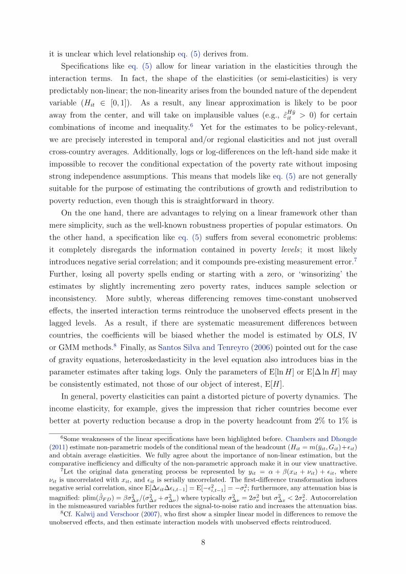
In general, poverty elasticities can paint a distorted picture of poverty dynamics. The
income elasticity, for example, gives the impression that richer countries become ever
better at poverty reduction because a drop in the poverty headcount from 2% to 1% is
6Some weaknesses of the linear specifications have been highlighted before. Chambers and Dhongde(2011) estimate non-parametric models of the conditional mean of the headcount (Hit = m(yit, Git)+εit)and obtain average elasticities. We fully agree about the importance of non-linear estimation, but thecomparative inefficiency and difficulty of the non-parametric approach make it in our view unattractive.
7Let the original data generating process be represented by yit = α + β(xit + νit) + εit, whereνit is uncorrelated with xit, and εit is serially uncorrelated. The first-difference transformation inducesnegative serial correlation, since E[∆εit∆εi,t−1] = E[−ε2i,t−1] = −σ2
ε ; furthermore, any attenuation bias is
magnified: plim(βFD) = βσ2∆x/(σ
2∆x +σ2
∆ν) where typically σ2∆ν = 2σ2
ν but σ2∆x < 2σ2
x. Autocorrelationin the mismeasured variables further reduces the signal-to-noise ratio and increases the attenuation bias.
8Cf. Kalwij and Verschoor (2007), who first show a simpler linear model in differences to remove theunobserved effects, and then estimate interaction models with unobserved effects reintroduced.
8
treated just the same as a drop from 50% to 25%. Recognizing this shortcoming, Klasen
and Misselhorn (2008) suggest to focus on absolute poverty changes instead. Removing
the log from the headcount in eq. (5) turns it into a model of semi-elasticities and alters
the interpretation.9 The coefficients now measure the percentage point change in the
population that is below the poverty line, expected for a given rate of change in income
or inequality. Likewise, eqs. (2) and (3) can be written as semi-elasticities by replacing
the inverse Mills ratio with the standard normal pdf. Contrary to elasticities, the semi-
elasticities converge to zero as mean income becomes large. Klasen and Misselhorn (2008)
also report that their models fit the data better and suggest that the specification in
absolute changes captures more of the inherent non-linearity. Even so, the fit is not
impressive (with an R2 up to 73%), considering the model stems from a decomposition
identity which should capture nearly all the variation short of measurement error.
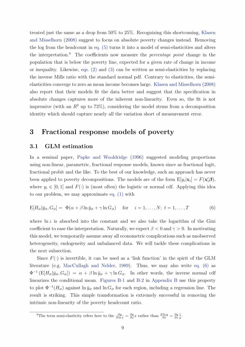
3 Fractional response models of poverty
3.1 GLM estimation
In a seminal paper, Papke and Wooldridge (1996) suggested modeling proportions
using non-linear, parametric, fractional response models, known since as fractional logit,
fractional probit and the like. To the best of our knowledge, such an approach has never
been applied to poverty decompositions. The models are of the form E[yi|xi] = F (x′iβ),
where yi ∈ [0, 1] and F (·) is (most often) the logistic or normal cdf. Applying this idea
to our problem, we may approximate eq. (1) with
E[Hit|yit, Git] = Φ(α + β ln yit + γ lnGit) for i = 1, . . . , N ; t = 1, . . . , T (6)
where ln z is absorbed into the constant and we also take the logarithm of the Gini
coefficient to ease the interpretation. Naturally, we expect β < 0 and γ > 0. In motivating
this model, we temporarily assume away all econometric complications such as unobserved
heterogeneity, endogeneity and unbalanced data. We will tackle these complications in
the next subsection.
Since F (·) is invertible, it can be used as a ‘link function’ in the spirit of the GLM
literature (e.g. MacCullagh and Nelder, 1989). Thus, we may also write eq. (6) as
Φ−1 (E[Hit|yit, Git]) = α + β ln yit + γ lnGit. In other words, the inverse normal cdf
linearizes the conditional mean. Figures B-1 and B-2 in Appendix B use this property
to plot Φ−1(Hit) against ln yit and lnGit for each region, including a regression line. The
result is striking. This simple transformation is extremely successful in removing the
intrinsic non-linearity of the poverty headcount ratio.
9The term semi-elasticity refers here to the ∂y∂ ln x = ∂y
∂xx rather than ∂ ln y∂x = ∂y
∂x1y .
9
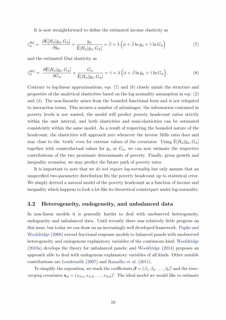
It is now straightforward to define the estimated income elasticity as
εHyit =∂E[Hit|yit, Git]
∂yit× yit
E[Hit|yit, Git]= β × λ
(α + β ln yit + γ lnGit
)(7)
and the estimated Gini elasticity as
εHGit =∂E[Hit|yit, Git]
∂Git
× Git
E[Hit|yit, Git]= γ × λ
(α + β ln yit + γ lnGit
). (8)
Contrary to log-linear approximations, eqs. (7) and (8) closely mimic the structure and
properties of the analytical elasticities based on the log-normality assumption in eqs. (2)
and (3). The non-linearity arises from the bounded functional form and is not relegated
to interaction terms. This secures a number of advantages: the information contained in
poverty levels is not wasted, the model will predict poverty headcount ratios strictly
within the unit interval, and both elasticities and semi-elasticities can be estimated
consistently within the same model. As a result of respecting the bounded nature of the
headcount, the elasticities will approach zero whenever the inverse Mills ratio does and
stay close to the ‘truth’ even for extreme values of the covariates. Using E[Hit|yit, Git]
together with counterfactual values for yit or Git, we can now estimate the respective
contributions of the two proximate determinants of poverty. Finally, given growth and
inequality scenarios, we may predict the future path of poverty rates.
It is important to note that we do not require log-normality but only assume that an
unspecified two-parameter distribution fits the poverty headcount up to statistical error.
We simply derived a natural model of the poverty headcount as a function of income and
inequality which happens to look a lot like its theoretical counterpart under log-normality.
3.2 Heterogeneity, endogeneity, and unbalanced data
In non-linear models it is generally harder to deal with unobserved heterogeneity,
endogeneity and unbalanced data. Until recently there was relatively little progress on
this issue, but today we can draw on an increasingly well developed framework. Papke and
Wooldridge (2008) extend fractional response models to balanced panels with unobserved
heterogeneity and endogenous explanatory variables of the continuous kind; Wooldridge
(2010a) develops the theory for unbalanced panels; and Wooldridge (2014) proposes an
approach able to deal with endogenous explanatory variables of all kinds. Other notable
contributions are Loudermilk (2007) and Ramalho et al. (2011).
To simplify the exposition, we stack the coefficients β = (β1, β2, . . . , βk)′ and the time-
varying covariates xit = (xit,1, xit,2, . . . , xit,k)′. The ideal model we would like to estimate
10
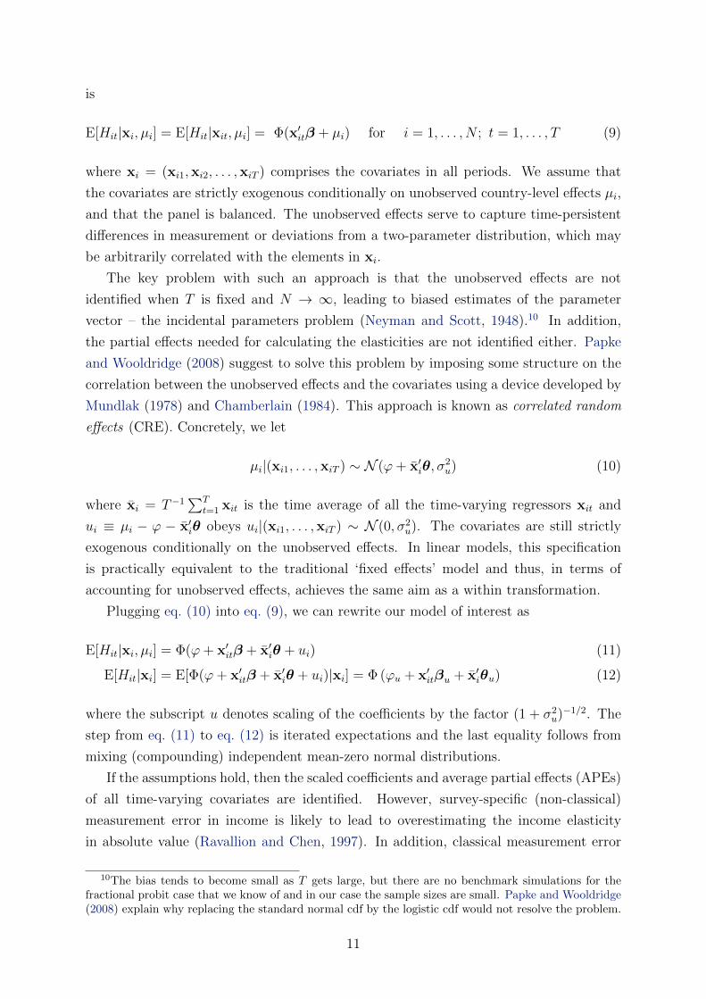
is
E[Hit|xi, µi] = E[Hit|xit, µi] = Φ(x′itβ + µi) for i = 1, . . . , N ; t = 1, . . . , T (9)
where xi = (xi1,xi2, . . . ,xiT ) comprises the covariates in all periods. We assume that
the covariates are strictly exogenous conditionally on unobserved country-level effects µi,
and that the panel is balanced. The unobserved effects serve to capture time-persistent
differences in measurement or deviations from a two-parameter distribution, which may
be arbitrarily correlated with the elements in xi.
The key problem with such an approach is that the unobserved effects are not
identified when T is fixed and N → ∞, leading to biased estimates of the parameter
vector – the incidental parameters problem (Neyman and Scott, 1948).10 In addition,
the partial effects needed for calculating the elasticities are not identified either. Papke
and Wooldridge (2008) suggest to solve this problem by imposing some structure on the
correlation between the unobserved effects and the covariates using a device developed by
Mundlak (1978) and Chamberlain (1984). This approach is known as correlated random
effects (CRE). Concretely, we let
µi|(xi1, . . . ,xiT ) ∼ N (ϕ+ x′iθ, σ2u) (10)
where xi = T−1∑T
t=1 xit is the time average of all the time-varying regressors xit and
ui ≡ µi − ϕ − x′iθ obeys ui|(xi1, . . . ,xiT ) ∼ N (0, σ2u). The covariates are still strictly
exogenous conditionally on the unobserved effects. In linear models, this specification
is practically equivalent to the traditional ‘fixed effects’ model and thus, in terms of
accounting for unobserved effects, achieves the same aim as a within transformation.
Plugging eq. (10) into eq. (9), we can rewrite our model of interest as
E[Hit|xi, µi] = Φ(ϕ+ x′itβ + x′iθ + ui) (11)
E[Hit|xi] = E[Φ(ϕ+ x′itβ + x′iθ + ui)|xi] = Φ (ϕu + x′itβu + x′iθu) (12)
where the subscript u denotes scaling of the coefficients by the factor (1 + σ2u)−1/2. The
step from eq. (11) to eq. (12) is iterated expectations and the last equality follows from
mixing (compounding) independent mean-zero normal distributions.
If the assumptions hold, then the scaled coefficients and average partial effects (APEs)
of all time-varying covariates are identified. However, survey-specific (non-classical)
measurement error in income is likely to lead to overestimating the income elasticity
in absolute value (Ravallion and Chen, 1997). In addition, classical measurement error
10The bias tends to become small as T gets large, but there are no benchmark simulations for thefractional probit case that we know of and in our case the sample sizes are small. Papke and Wooldridge(2008) explain why replacing the standard normal cdf by the logistic cdf would not resolve the problem.
11
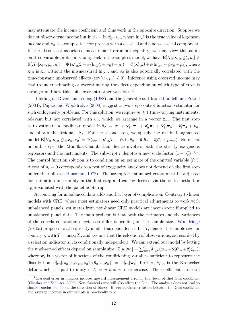
may attenuate the income coefficient and thus work in the opposite direction. Suppose we
do not observe true income but ln yit = ln y∗it+υit, where ln y∗it is the true value of log-mean
income and υit is a composite error process with a classical and a non-classical component.
In the absence of associated measurement error in inequality, we may view this as an
omitted variable problem. Going back to the simplest model, we have E[Hit|x1it, y∗it, µi] 6=
E[Hit|x1it, yit, µi] = Φ (x′1itβ + ψ(ln y∗it + υit) + µi) = Φ(x′1itβ+ψ ln yit+ψυit+µi), where
x1it is xit without the mismeasured ln yit, and υit is also potentially correlated with the
time-constant unobserved effects (cov(υit, µi) 6= 0). Inference using observed income may
lead to underestimating or overestimating the effect depending on which type of error is
stronger and how this spills over into other variables.11
Building on Rivers and Vuong (1988) and the general result from Blundell and Powell
(2004), Papke and Wooldridge (2008) suggest a two-step control function estimator for
such endogeneity problems. For this solution, we require m ≥ 1 time-varying instruments,
relevant but not correlated with υit, which we arrange in a vector zit. The first step
is to estimate a log-linear model ln yit = π0 + x′1itπ1 + z′itπ2 + x′1iπ3 + z′iπ4 + νit,
and obtain the residuals νit. For the second step, we specify the residual-augmented
model E[Hit|x1it, yit, zit, νit] = Φ (ϕr + x′1itβr + ψr ln yit + x′iθr + z′iζr + ρrνit). Note that
in both steps, the Mundlak-Chamberlain device involves both the strictly exogenous
regressors and the instruments. The subscript r denotes a new scale factor (1 + σ2r)−1/2.
The control function solution is to condition on an estimate of the omitted variable (νit).
A test of ρr = 0 corresponds to a test of exogeneity and does not depend on the first step
under the null (see Hausman, 1978). The asymptotic standard errors must be adjusted
for estimation uncertainty in the first step and can be derived via the delta method or
approximated with the panel bootstrap.
Accounting for unbalanced data adds another layer of complication. Contrary to linear
models with CRE, where most estimators need only practical adjustments to work with
unbalanced panels, estimates from non-linear CRE models are inconsistent if applied to
unbalanced panel data. The main problem is that both the estimates and the variances
of the correlated random effects can differ depending on the sample size. Wooldridge
(2010a) proposes to also directly model this dependence. Let Ti denote the sample size for
country i, with T = maxi Ti; and assume that the selection of observations, as recorded by
a selection indicator sit, is conditionally independent. We can extend our model by letting
the unobserved effects depend on sample size: E[µi|wi] =∑T
n=1 δTi,n(ϕrn+ x′iθrn+ z′iζrn),
where wi is a vector of functions of the conditioning variables sufficient to represent the
distribution D[µi|(sit, sitx1it, sit ln yit, sitzit)] = D[µi|wi]; further, δTi,n is the Kronecker
delta which is equal to unity if Ti = n and zero otherwise. The coefficients are still
11Classical error in incomes induces upward measurement error in the (level of the) Gini coefficient(Chesher and Schluter, 2002). Non-classical error will also affect the Gini. The analysis does not lead tosimple conclusions about the direction of biases. However, the correlation between the Gini coefficientand average incomes in our sample is practically zero.
12
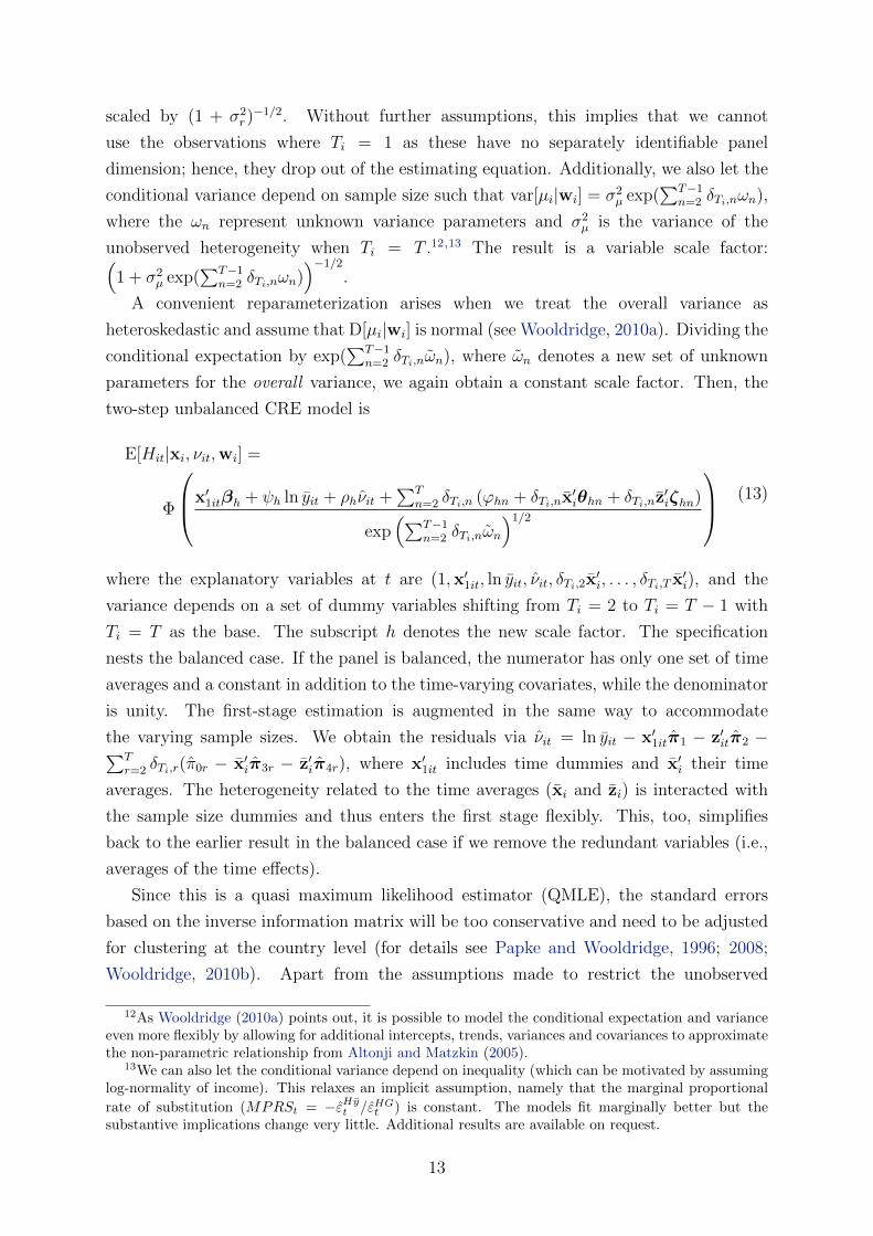
scaled by (1 + σ2r)−1/2. Without further assumptions, this implies that we cannot
use the observations where Ti = 1 as these have no separately identifiable panel
dimension; hence, they drop out of the estimating equation. Additionally, we also let the
conditional variance depend on sample size such that var[µi|wi] = σ2µ exp(
∑T−1n=2 δTi,nωn),
where the ωn represent unknown variance parameters and σ2µ is the variance of the
unobserved heterogeneity when Ti = T .12,13 The result is a variable scale factor:(1 + σ2
µ exp(∑T−1
n=2 δTi,nωn))−1/2
.
A convenient reparameterization arises when we treat the overall variance as
heteroskedastic and assume that D[µi|wi] is normal (see Wooldridge, 2010a). Dividing the
conditional expectation by exp(∑T−1
n=2 δTi,nωn), where ωn denotes a new set of unknown
parameters for the overall variance, we again obtain a constant scale factor. Then, the
two-step unbalanced CRE model is
E[Hit|xi, νit,wi] =
Φ
x′1itβh + ψh ln yit + ρhνit +
∑Tn=2 δTi,n (ϕhn + δTi,nx
′iθhn + δTi,nz
′iζhn)
exp(∑T−1
n=2 δTi,nωn
)1/2
(13)
where the explanatory variables at t are (1,x′1it, ln yit, νit, δTi,2x′i, . . . , δTi,T x
′i), and the
variance depends on a set of dummy variables shifting from Ti = 2 to Ti = T − 1 with
Ti = T as the base. The subscript h denotes the new scale factor. The specification
nests the balanced case. If the panel is balanced, the numerator has only one set of time
averages and a constant in addition to the time-varying covariates, while the denominator
is unity. The first-stage estimation is augmented in the same way to accommodate
the varying sample sizes. We obtain the residuals via νit = ln yit − x′1itπ1 − z′itπ2 −∑Tr=2 δTi,r(π0r − x′iπ3r − z′iπ4r), where x′1it includes time dummies and x′i their time
averages. The heterogeneity related to the time averages (xi and zi) is interacted with
the sample size dummies and thus enters the first stage flexibly. This, too, simplifies
back to the earlier result in the balanced case if we remove the redundant variables (i.e.,
averages of the time effects).
Since this is a quasi maximum likelihood estimator (QMLE), the standard errors
based on the inverse information matrix will be too conservative and need to be adjusted
for clustering at the country level (for details see Papke and Wooldridge, 1996; 2008;
Wooldridge, 2010b). Apart from the assumptions made to restrict the unobserved
12As Wooldridge (2010a) points out, it is possible to model the conditional expectation and varianceeven more flexibly by allowing for additional intercepts, trends, variances and covariances to approximatethe non-parametric relationship from Altonji and Matzkin (2005).
13We can also let the conditional variance depend on inequality (which can be motivated by assuminglog-normality of income). This relaxes an implicit assumption, namely that the marginal proportional
rate of substitution (MPRSt = −εHyt /εHGt ) is constant. The models fit marginally better but thesubstantive implications change very little. Additional results are available on request.
13
heterogeneity and endogeneity, fractional probit only requires correct specification of
the conditional mean, irrespective of the true distribution of the dependent variable
(Gourieroux, Monfort, and Trognon, 1984). Hence, it is as robust as non-linear least
squares but potentially more efficient.14
We still need to define the average partial effects (APEs) and the relevant elasticities.
Both can be derived from the average structural function (ASF) computed over the
selected sample (see Blundell and Powell, 2004; Wooldridge, 2010a), which highlights that
in fact only the APEs of time-varying covariates are identified. Let the linear predictors
inside the cumulative normal be m′it1ξ1 for the main equation and m′it2ξ2 for the variance
equation. Then, ASF(x1t, . . . ,xNt) = N−1∑N
i=1 Φ(m′it1ξ1/exp(m′it2ξ2)1/2
), where xit
refers to all time-varying covariates including mismeasured income, and the ξ coefficients
are the scaled QMLE estimates. We need to average over the cross-sectional dimension
in order to get rid of the unobserved effects, varying panel sizes, and endogeneity due to
measurement error. The APE at time t of a particular continuous variable is simply the
derivative of the ASF with respect to that variable. We later plug in interesting values
for the xit and obtain the corresponding APEs.
By analogy, the (average) elasticity with respect to an element xk of xit, assuming xk
is in logs and does not show up in the variance equation, is found to be
εHxkt = βk ×N−1
N∑
i=1
exp(−m′it2ξ2/2
)λ(m′it1ξ1/exp(m′it2ξ2)1/2
)(14)
and the semi-elasticity (ηHxkt ) is the derivative of the ASF with respect to xk; that is,
the average partial effect (APE). It can be obtained by simply replacing λ(·) with φ(·) in
eq. (14) above. Since the surveys are irregularly spaced and often cover only parts of a
given year, it is not straightforward to obtain and describe the evolution of the ASF over
time. Hence, we usually also average over time in order to obtain a single scale factor
and a single APE for each variable of interest.
The basic structure is exactly the same as in the simpler versions derived in the
previous section with the addition of a variance equation adjusting for the degree of
unbalancedness. If the panel is balanced, the non-redundant sums inside the linear
predictors simplify and we again obtain the CRE analogues of eqs. (7) and (8).
14This is a complicated model to fit but it can be estimated by any software that has a heteroskedasticprobit implementation without any restrictions on the dependent variable (Wooldridge, 2010a). However,most implementations (e.g. Stata’s hetprob) only allow binary dependent variables. We implementthe estimator in a new module called fhetprob with analytic first and second derivatives, see www.
richard-bluhm.com/data/. Since the arrival of Stata 14, end users may also use the built-in commandfracreg probit with properly defined heteroskedastic terms to estimate our models.
14
4 Data
Based on the World Bank’s PovcalNet database15, we compile a new and comprehensive
data set consisting of 809 nationally-representative surveys spanning 124 countries from
1981 to 2010.16 Smaller panels of this data have been used in previous studies (e.g.
Chambers and Dhongde, 2011; Kalwij and Verschoor, 2007; Adams, 2004) and the World
Bank’s methodology is described in more detail in Chen and Ravallion (2010). Here we
only briefly summarize the main features.
All data originate from household surveys. We consider poverty headcount ratios (Hit)
under two different poverty lines (z) widely used for international comparisons: $2 a day
($60.80 a month) and $1.25 a day ($38 a month). The latter is typically used to assess
extreme poverty. In addition to these poverty rates, the data contain monthly per capita
household income or consumption expenditures (yit)17, the Gini coefficient of inequality
(Git) for income or consumption expenditures, and the size of the surveyed population
(popit). We generate two dummy variables indicating whether welfare is measured by
income or consumption, and whether it is reported at the level of units (households)
or groups (deciles or finer quantiles). Reported poverty is typically lower in income
surveys than consumption surveys, and the availability of grouped versus unit-level data
in PovcalNet may proxy for other systematic survey differences. About 63% of the data
come from expenditure surveys and about 74% are estimated from grouped data. All
monetary quantities are in constant international dollars at 2005 PPP-adjusted prices.
Three large countries, China, India and Indonesia, do not conduct nationally
representative surveys, but instead report urban and rural data separately. To construct
national series we simply weigh the poverty and income data using the relative
urban/rural population shares. As to the Gini coefficient, since it is not subgroup-
decomposable, we estimate a national Gini coefficient via an approximation due to Young
(2011), based on a mixture of two log-normal distributions.18 If only one urban or rural
survey is available in any given year, we usually drop the survey, except in the case of
Argentina where urbanization is near or above 90% for most of the sampled period and
we thus consider the urban series nationally representative. The result is an unbalanced
panel of 124 countries spanning 30 years, with an average time series length (T ) of about
6.5 surveys for a total of 809 observations. Table 1 provides summary statistics for
15The data is publicly available at http://iresearch.worldbank.org/PovcalNet (we use the 2005PPP version).
16Supporting materials and the panel data set are available at www.richard-bluhm.com/data/.17Computed as a simple per capita average without equivalence scaling.18PovcalNet omits weighting some recent data. To use a single consistent method, we apply Young’s
formula in all cases where separate urban and rural surveys are combined. The approximation is very
accurate. The formula is G =∑Ki=1
∑Kj=1
sisj yiY
(2K
[ln yi−ln yj+ 1
2σ2i + 1
2σ2j
(σ2i +σ2
j )1/2
]− 1)
where K is the total
number of subgroups, si is the population share of the i-th subgroup, yi is mean income, σ2i is the
variance, and Y is the population-weighted mean income across all subgroups.
15
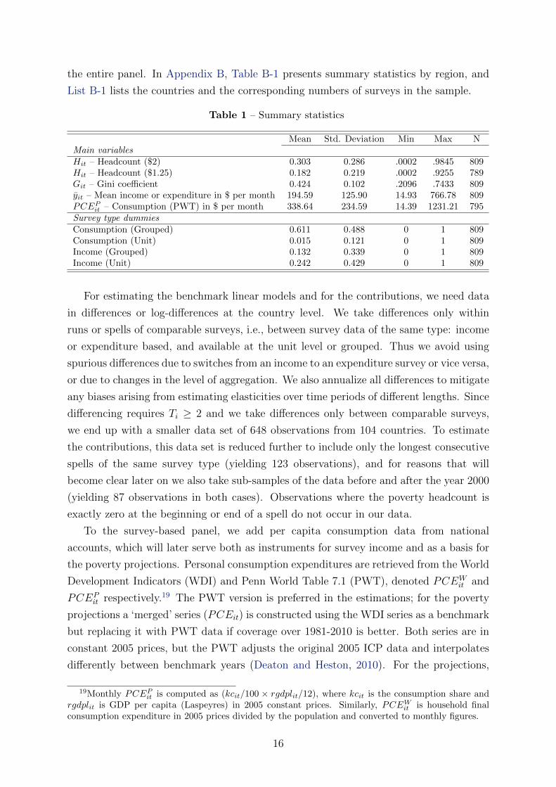
the entire panel. In Appendix B, Table B-1 presents summary statistics by region, and
List B-1 lists the countries and the corresponding numbers of surveys in the sample.
Table 1 – Summary statistics
Mean Std. Deviation Min Max NMain variablesHit – Headcount ($2) 0.303 0.286 .0002 .9845 809Hit – Headcount ($1.25) 0.182 0.219 .0002 .9255 789Git – Gini coefficient 0.424 0.102 .2096 .7433 809yit – Mean income or expenditure in $ per month 194.59 125.90 14.93 766.78 809PCEPit – Consumption (PWT) in $ per month 338.64 234.59 14.39 1231.21 795Survey type dummiesConsumption (Grouped) 0.611 0.488 0 1 809Consumption (Unit) 0.015 0.121 0 1 809Income (Grouped) 0.132 0.339 0 1 809Income (Unit) 0.242 0.429 0 1 809
For estimating the benchmark linear models and for the contributions, we need data
in differences or log-differences at the country level. We take differences only within
runs or spells of comparable surveys, i.e., between survey data of the same type: income
or expenditure based, and available at the unit level or grouped. Thus we avoid using
spurious differences due to switches from an income to an expenditure survey or vice versa,
or due to changes in the level of aggregation. We also annualize all differences to mitigate
any biases arising from estimating elasticities over time periods of different lengths. Since
differencing requires Ti ≥ 2 and we take differences only between comparable surveys,
we end up with a smaller data set of 648 observations from 104 countries. To estimate
the contributions, this data set is reduced further to include only the longest consecutive
spells of the same survey type (yielding 123 observations), and for reasons that will
become clear later on we also take sub-samples of the data before and after the year 2000
(yielding 87 observations in both cases). Observations where the poverty headcount is
exactly zero at the beginning or end of a spell do not occur in our data.
To the survey-based panel, we add per capita consumption data from national
accounts, which will later serve both as instruments for survey income and as a basis for
the poverty projections. Personal consumption expenditures are retrieved from the World
Development Indicators (WDI) and Penn World Table 7.1 (PWT), denoted PCEWit and
PCEPit respectively.19 The PWT version is preferred in the estimations; for the poverty
projections a ‘merged’ series (PCEit) is constructed using the WDI series as a benchmark
but replacing it with PWT data if coverage over 1981-2010 is better. Both series are in
constant 2005 prices, but the PWT adjusts the original 2005 ICP data and interpolates
differently between benchmark years (Deaton and Heston, 2010). For the projections,
19Monthly PCEPit is computed as (kcit/100 × rgdplit/12), where kcit is the consumption share andrgdplit is GDP per capita (Laspeyres) in 2005 constant prices. Similarly, PCEWit is household finalconsumption expenditure in 2005 prices divided by the population and converted to monthly figures.
16
we also use population estimates covering the period 2010-2030 from the World Bank’s
Health, Nutrition and Population Statistics database.
5 Results
5.1 Regressions
Table 2 presents our main results, with each specification progressively addressing more
estimation issues: unobserved effects, unbalancedness and measurement error, in that
order. All specifications include time averages a la Mundlak to proxy for measurement
differences across countries (unobserved effects), and survey type dummies (consumption
or income, grouped or unit data) to control for measurement differences across surveys.
In addition, a full set of year dummies allows for unspecified common time effects.
Column (1) includes correlated random effects but ignores unbalancedness. As
expected, the coefficient on average income is negative and the coefficient on inequality
is positive. Since the estimated coefficients are arbitrarily scaled, the adjacent column
reports average partial effects (APEs); the scale factor is reported separately in the
bottom panel. The APEs in column (1) are interpreted as average semi-elasticities :
income growth of one percent results in a reduction in the number of poor by 0.284
percentage points ; and a Gini increase of one percent corresponds to an increase in
the number of poor by 0.232 percentage points. As for elasticities, the average income
elasticity across the entire estimation sample is about −1.83 (SE = 0.084) and the average
Gini elasticity is about 1.5 (SE = 0.167). For instance, one percent income growth would
lead to about a 1.83 percent reduction in poverty. These two estimates are located near
the lower end of the figures typically found in the literature.20
Our first specification could be biased due to the strong unbalancedness of the panel
and the presence of time-varying measurement error in income and inequality. Column
(2) addresses unbalancedness by including panel size dummies, interactions of the time
averages with the panel size dummies, and a separate variance equation. We consider
this our best specification without correcting for measurement error. The substantive
conclusions change very little. The APE of income is virtually unchanged and the APE
of inequality increases by less than one standard error. Tentatively, we conclude that
varying sample sizes introduce little bias on average. Nonetheless, they may still have
non-negligible effects on the (semi-)elasticities at particular points in time.
Our preferred specification, column (3), is the empirical counterpart of the two-
20The typical range for the income elasticity in earlier studies is from about -2 to -5, while the rangefor the Gini elasticity is much wider. Newer studies suggest the income elasticity is closer to -2. This islargely owed to parameter instability in linear approximations and changing data coverage. However, asChambers and Dhongde (2011) report, estimates of the income elasticity using the 2005 PPPs are alsouniversally lower (in absolute value) than estimates based on the earlier 1993 PPPs.
17
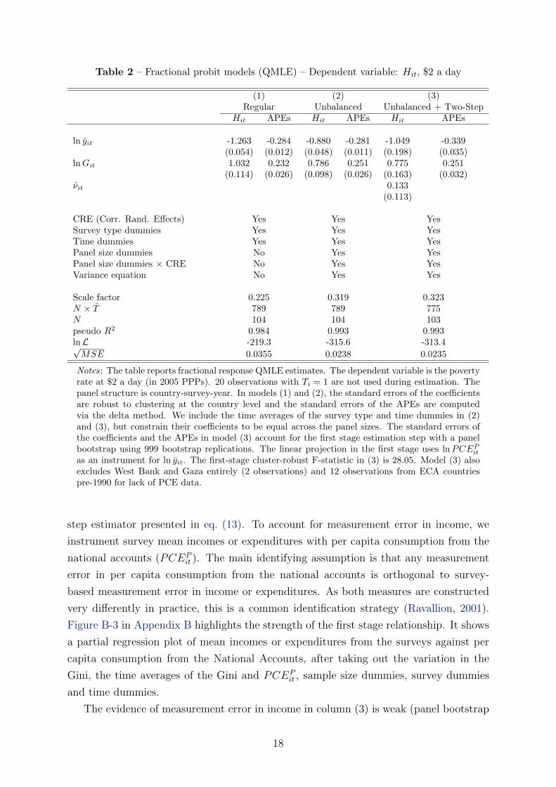
Table 2 – Fractional probit models (QMLE) – Dependent variable: Hit, $2 a day
(1) (2) (3)Regular Unbalanced Unbalanced + Two-Step
Hit APEs Hit APEs Hit APEs
ln yit -1.263 -0.284 -0.880 -0.281 -1.049 -0.339(0.054) (0.012) (0.048) (0.011) (0.198) (0.035)
lnGit 1.032 0.232 0.786 0.251 0.775 0.251(0.114) (0.026) (0.098) (0.026) (0.163) (0.032)
νit 0.133(0.113)
CRE (Corr. Rand. Effects) Yes Yes YesSurvey type dummies Yes Yes YesTime dummies Yes Yes YesPanel size dummies No Yes YesPanel size dummies × CRE No Yes YesVariance equation No Yes Yes
Scale factor 0.225 0.319 0.323N × T 789 789 775N 104 104 103pseudo R2 0.984 0.993 0.993lnL -219.3 -315.6 -313.4√MSE 0.0355 0.0238 0.0235
Notes: The table reports fractional response QMLE estimates. The dependent variable is the povertyrate at $2 a day (in 2005 PPPs). 20 observations with Ti = 1 are not used during estimation. Thepanel structure is country-survey-year. In models (1) and (2), the standard errors of the coefficientsare robust to clustering at the country level and the standard errors of the APEs are computedvia the delta method. We include the time averages of the survey type and time dummies in (2)and (3), but constrain their coefficients to be equal across the panel sizes. The standard errors ofthe coefficients and the APEs in model (3) account for the first stage estimation step with a panelbootstrap using 999 bootstrap replications. The linear projection in the first stage uses lnPCEPitas an instrument for ln yit. The first-stage cluster-robust F-statistic in (3) is 28.05. Model (3) alsoexcludes West Bank and Gaza entirely (2 observations) and 12 observations from ECA countriespre-1990 for lack of PCE data.
step estimator presented in eq. (13). To account for measurement error in income, we
instrument survey mean incomes or expenditures with per capita consumption from the
national accounts (PCEPit ). The main identifying assumption is that any measurement
error in per capita consumption from the national accounts is orthogonal to survey-
based measurement error in income or expenditures. As both measures are constructed
very differently in practice, this is a common identification strategy (Ravallion, 2001).
Figure B-3 in Appendix B highlights the strength of the first stage relationship. It shows
a partial regression plot of mean incomes or expenditures from the surveys against per
capita consumption from the National Accounts, after taking out the variation in the
Gini, the time averages of the Gini and PCEPit , sample size dummies, survey dummies
and time dummies.
The evidence of measurement error in income in column (3) is weak (panel bootstrap
18
t-stat ≈ 1.18). If we ignore first-stage sampling error, the evidence is stronger (cluster-
robust t-stat ≈ 1.69).21 The APE of income is considerably larger in absolute value than
in the previous two specifications, though the APE of inequality is not. We tentatively
conclude that the coefficient of income in models (1) and (2) is moderately attenuated.
This would suggest that classical attenuation bias is more of a problem than systematic
survey bias, but we cannot rule out that more complex error structures are at play.
Like the APE, the average income elasticity of poverty in model (3) is larger in
absolute value (¯εHy ≈ −2.21, SE = 0.156). Income growth of one percent leads to a
0.339 percentage point or 2.21 percent reduction in the number of poor, on average. The
inequality APE and elasticity remain about the same (¯εHG ≈ 1.64, SE = 0.188). Actually,
there may also be non-negligible measurement error in observed inequality as measured
by the Gini coefficient. However, since inequality is estimated from household surveys
and estimates based on alternative sources such as tax records are not available on a
cross-country basis, we are lacking a corresponding instrument for the Gini coefficient.
At first sight, all three models may suggest that the effect of income growth is only
moderately stronger than the effect of inequality when the other variable is held constant.
This does not imply that both variables have the same scope for change, or have to change
independently for that matter. For now, we only estimate the impact of each component
and not its contribution to overall poverty reduction. While there is substantial variation
in inequality, it shows no systematic trend over the sample period from 1981 to 2010.22
In contrast, incomes and expenditures have increased substantially in all regions over
the same time span (see Table B-3 in Appendix B). Yet, the effect of income growth
is not constant. In these models, it depends strongly on the levels of inequality and
income. There is a ‘double dividend’ to improvements in distribution (Bourguignon,
2003) and substantial heterogeneity in the estimated poverty (semi-)elasticities across
time and space – an issue to which we return shortly.
Perhaps the most striking fact about all three specifications is how well they fit.23
The last row of Table 2 shows the square root of the mean squared residual for each
column. We predict the observed poverty headcount for each country-year with about
three and a half percentage points accuracy in the first model, and with better than two
and a half percentage points accuracy in the next two. This is what one would expect
from a well-defined decomposition. A simple pseudo-R2 measure, the squared correlation
between the observed and fitted values, suggests near perfect fit (R2 > 0.98). Figure 1
21As mentioned earlier, the Hausman (1978) test does not depend on the first stage under the null.22In a simple regression of the Gini coefficient on time, we fail to reject the null hypothesis that the
time trend is zero (cluster-robust t-stat ≈ 0.07 and p > 0.94).23To examine if there is evidence of omitted non-linearity, we add squares (m′it1ξ1)2 and cubes
(m′it1ξ1)3 of the linear predictors in columns (1) and (2) for a RESET-type test as suggested by Papkeand Wooldridge (1996). In column (1), this yields a robust χ2
2-statistic of 4.65 (p = 0.098), giving noreason for concern; in column (2), the statistic is χ2
2 = 9.15 (p = 0.010), signaling missing non-linearity.We see no theoretical rationale, though, to enter additional powers or interactions into the model.
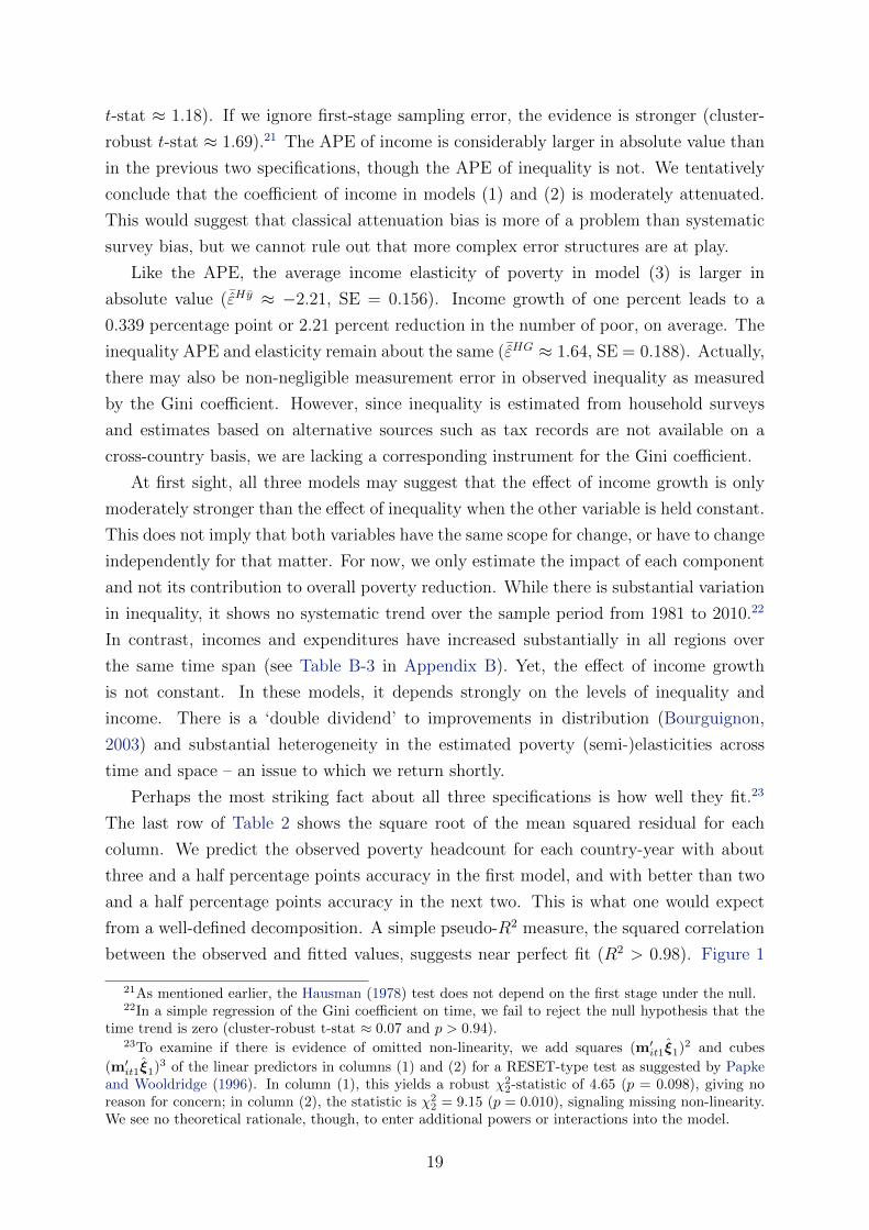
19
illustrates this point and shows the shape of the estimated effects. Using our preferred
specification, we plot both the observed headcount and the predicted headcount over the
range of observed mean income or expenditures (left panel) and inequality (right panel).
The quality of the non-linear approach is apparent. The fit is very close at either bound
(near unity or near zero) and the model predicts no nonsensical values. Furthermore, the
entire range of variation of the observed values is covered by the model predictions.
Figure 1 – Data versus fitted values, preferred specification, $2 a day
0.00
0.25
0.50
0.75
1.00
0 200 400 600 800Mean income (yit)
Pov
erty
Hea
dco
unt
(Hit
)
0.00
0.25
0.50
0.75
1.00
0.2 0.4 0.6Gini (Git)
Pov
erty
Hea
dco
unt
(Hit
)
E[H|X]
Actual
Notes: Illustration of the model fit from the estimates presented in column (3) of Table 2. The leftpanel shows the observed poverty rates (actual) and predicted poverty rates (E[H|X]) over meanincomes; the right panel plots both over the Gini coefficient.
For comparison, Table B-2 in Appendix B reproduces the linear approach so common
in the literature. As is typical for such comparisons, linearly and non-linearly estimated
elasticities are very similar on average. Yet the various linear estimates suffer from
the expected problems (see Section 2). First, the step from within-transformed data
in column (1) to annualized differences in the following columns seems to worsen the
impact of measurement error and attenuate the income effect. Second, the models with
interaction terms do not fit nearly as well as the fractional probit models and many
coefficients are insignificant. Third, the two-step GMM estimates of the interaction
models are unstable and unable to convincingly reverse the attenuation effect. The
last model, which mimics the preferred specification of Kalwij and Verschoor (2007),
even implies a negative Gini elasticity, and all coefficients are estimated with great
imprecision. In sum, these models perform poorly in comparison to the fractional
response counterparts and are unlikely to produce reliable estimates over a wide range of
circumstances.
20
5.2 Impacts
The strength of the fractional response approach lies in its ability to deliver precise
and unbiased estimates of effects other than the overall mean response. Table 3 and
Table 4 illustrate this point by estimating income and Gini elasticities (Panel a)) and
semi-elasticities (Panel b)) over different time periods for six large geographic regions.
The elasticities are computed according to eq. (14) by plugging in time-period and region-
specific averages of mean income (ln yit) and inequality (lnGit), and then averaging over
the entire sample; the semi-elasticities are computed analogously. Standard errors are
computed via a panel bootstrap and thus take into account the sampling uncertainty of
the first stage.
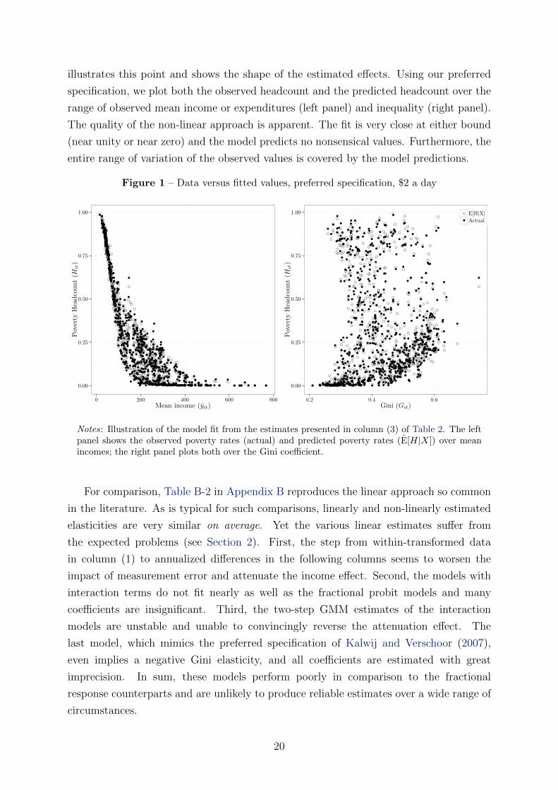
Table 3 – Income elasticities and semi-elasticities, $2 a day, by region
Time period
1981–1989 1990–1994 1995–1999 2000–2004 2005–2010
Panel a) Regional income elasticities
East Asia and Pacific -0.991 -1.029 -1.237 -1.139 -1.578(0.030) (0.033) (0.055) (0.043) (0.101)
Eastern Europe and Central Asia -4.358 -2.892 -2.700 -2.846 -3.304(0.555) (0.309) (0.277) (0.304) (0.384)
Latin America and Caribbean -2.284 -2.374 -2.425 -2.349 -2.985(0.243) (0.257) (0.271) (0.258) (0.366)
Middle East and North Africa -2.176 -2.116 -2.024 -1.966 -2.501(0.203) (0.188) (0.168) (0.161) (0.246)
South Asia -0.548 -0.629 -0.810 -1.024 -1.192(0.053) (0.048) (0.030) (0.032) (0.046)
Sub-Saharan Africa -0.831 -0.437 -0.436 -0.592 -0.632(0.027) (0.039) (0.040) (0.035) (0.033)
Panel b) Regional income semi-elasticities
East Asia and Pacific -0.568 -0.573 -0.585 -0.583 -0.552(0.034) (0.036) (0.046) (0.042) (0.051)
Eastern Europe and Central Asia -0.031 -0.214 -0.260 -0.225 -0.134(0.008) (0.015) (0.020) (0.015) (0.010)
Latin America and Caribbean -0.374 -0.348 -0.334 -0.355 -0.194(0.028) (0.025) (0.024) (0.026) (0.013)
Middle East and North Africa -0.405 -0.422 -0.447 -0.463 -0.313(0.034) (0.037) (0.042) (0.043) (0.024)
South Asia -0.418 -0.458 -0.526 -0.572 -0.585(0.023) (0.019) (0.022) (0.036) (0.044)
Sub-Saharan Africa -0.532 -0.354 -0.353 -0.440 -0.459(0.024) (0.020) (0.020) (0.015) (0.015)
Notes: The table reports regional income elasticities in panel a) and regional income semi-elasticitiesin panel b). The estimates are computed by plugging period and region-specific averages of meanincome and inequality into eq. (14) or its semi-elasticity counterpart and then averaging over theentire sample. Standard errors are obtained via a panel bootstrap using 999 replications.
There are considerable regional and temporal differences in the estimated income
elasticities. As the theoretical derivations in Section 2 show, the origin of the
21
heterogeneity of elasticities is essentially mechanical: it is a consequence of heterogeneity
in incomes and inequality. More affluent regions (Eastern Europe and Central Asia,
Latin America and the Caribbean, and the Middle East and North Africa) have higher
income elasticities than poorer regions (East Asia and Pacific, South Asia, and Sub-
Saharan Africa). Income dynamics over time are also clearly visible. In Eastern Europe
and Central Asia, for example, income is comparatively high before the post-communist
transition, sharply collapses through the 1990s, and recovers during the 2000s. Compared
to earlier results (e.g. Kalwij and Verschoor, 2007), we find markedly higher average
income elasticities in more affluent regions and lower elasticities in poorer regions. All
standard errors in Table 3 are small compared to the point estimates and remain small
for regions with extreme values (like Sub-Saharan Africa, with its very low incomes and
above average inequalities in the 1980s).
Panel b) presents the region and time specific income semi-elasticities of poverty.
There the picture is reversed. Comparatively affluent regions have fewer people near the
poverty line, and thus the poverty reduction potential from a one percent increase in
incomes is much smaller in terms of the numbers lifted out of poverty. This pattern is
(again) best visible in Eastern Europe and Central Asia, where absolute poverty at the
$2 a day poverty line is almost non-existent just before the post-communist transition,
but rises sharply in the 1990s as incomes decline. Correspondingly, the semi-elasticity is
close to zero in the 1980s but then increases as more people fall into poverty. Likewise,
the biggest poverty reduction potential in 2005-2010 was in East Asia, South Asia, and
Sub-Saharan Africa. This highlights an important point. For development policy, what
we really care about is the percent of the population lifted out of poverty rather than the
percentage reduction in the poverty rate.
The region and time specific Gini elasticities in Panel a) of Table 4 show where the
potential of redistributive policies in terms of proportionate reductions in the poverty
headcount was largest over the last three decades. Unsurprisingly, these regions are
Eastern Europe and Central Asia, Latin America and the Caribbean, and the Middle East
and North Africa – all of which have above average inequality. Sub-Saharan Africa starts
out with high inequality in the 1980s24 but incomes are very low relative to the poverty
line, so that the Gini elasticity is small. This is the flip side of the dependency on initial
levels: countries can be so poor and unequal that the immediate effects of equalization
and income growth on relative changes in the poverty headcount are relatively small.
Again, though, the semi-elasticities presented in Panel b) overhaul the picture. There
the relative position of poorer and richer countries is reversed. The potential for reducing
poverty through redistribution in terms of percent of the population that is poor was
larger in poorer regions throughout the entire period from 1981 to 2010.
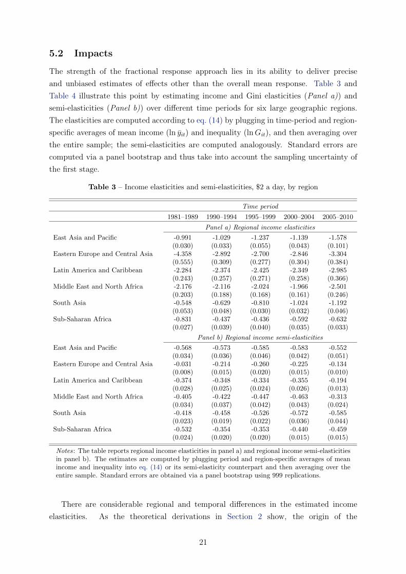
The ‘double dividend’ of reductions in inequality is illustrated in Figure 2 by graphing
24The population-weighted mean Gini in the 1980s is 0.4608.
22
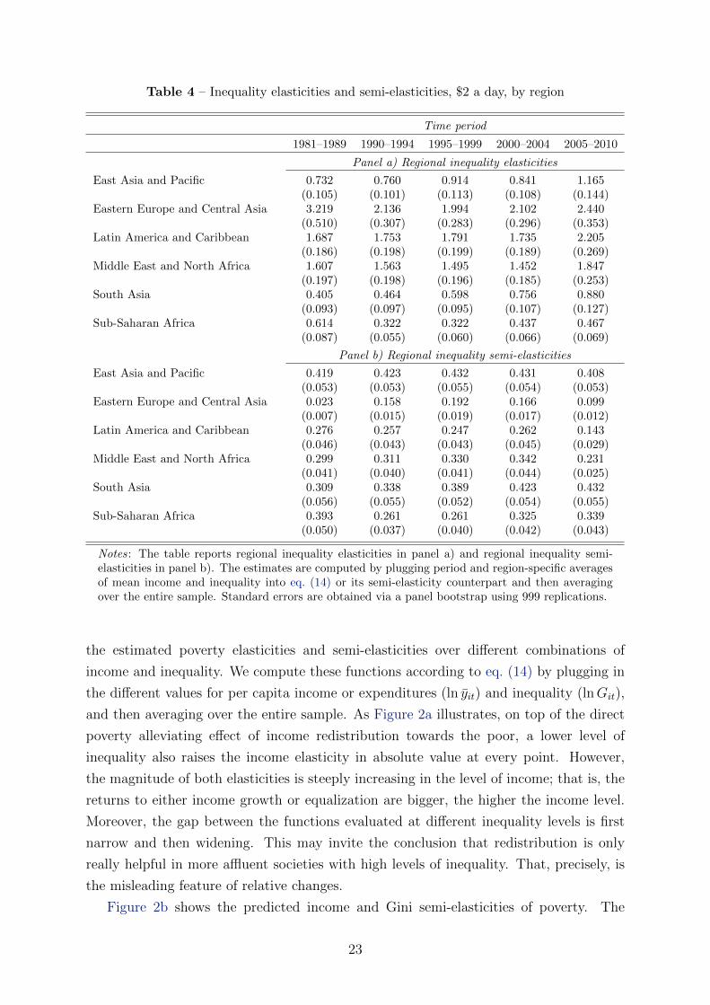
Table 4 – Inequality elasticities and semi-elasticities, $2 a day, by region
Time period
1981–1989 1990–1994 1995–1999 2000–2004 2005–2010
Panel a) Regional inequality elasticities
East Asia and Pacific 0.732 0.760 0.914 0.841 1.165(0.105) (0.101) (0.113) (0.108) (0.144)
Eastern Europe and Central Asia 3.219 2.136 1.994 2.102 2.440(0.510) (0.307) (0.283) (0.296) (0.353)
Latin America and Caribbean 1.687 1.753 1.791 1.735 2.205(0.186) (0.198) (0.199) (0.189) (0.269)
Middle East and North Africa 1.607 1.563 1.495 1.452 1.847(0.197) (0.198) (0.196) (0.185) (0.253)
South Asia 0.405 0.464 0.598 0.756 0.880(0.093) (0.097) (0.095) (0.107) (0.127)
Sub-Saharan Africa 0.614 0.322 0.322 0.437 0.467(0.087) (0.055) (0.060) (0.066) (0.069)
Panel b) Regional inequality semi-elasticities
East Asia and Pacific 0.419 0.423 0.432 0.431 0.408(0.053) (0.053) (0.055) (0.054) (0.053)
Eastern Europe and Central Asia 0.023 0.158 0.192 0.166 0.099(0.007) (0.015) (0.019) (0.017) (0.012)
Latin America and Caribbean 0.276 0.257 0.247 0.262 0.143(0.046) (0.043) (0.043) (0.045) (0.029)
Middle East and North Africa 0.299 0.311 0.330 0.342 0.231(0.041) (0.040) (0.041) (0.044) (0.025)
South Asia 0.309 0.338 0.389 0.423 0.432(0.056) (0.055) (0.052) (0.054) (0.055)
Sub-Saharan Africa 0.393 0.261 0.261 0.325 0.339(0.050) (0.037) (0.040) (0.042) (0.043)
Notes: The table reports regional inequality elasticities in panel a) and regional inequality semi-elasticities in panel b). The estimates are computed by plugging period and region-specific averagesof mean income and inequality into eq. (14) or its semi-elasticity counterpart and then averagingover the entire sample. Standard errors are obtained via a panel bootstrap using 999 replications.
the estimated poverty elasticities and semi-elasticities over different combinations of
income and inequality. We compute these functions according to eq. (14) by plugging in
the different values for per capita income or expenditures (ln yit) and inequality (lnGit),
and then averaging over the entire sample. As Figure 2a illustrates, on top of the direct
poverty alleviating effect of income redistribution towards the poor, a lower level of
inequality also raises the income elasticity in absolute value at every point. However,
the magnitude of both elasticities is steeply increasing in the level of income; that is, the
returns to either income growth or equalization are bigger, the higher the income level.
Moreover, the gap between the functions evaluated at different inequality levels is first
narrow and then widening. This may invite the conclusion that redistribution is only
really helpful in more affluent societies with high levels of inequality. That, precisely, is
the misleading feature of relative changes.
Figure 2b shows the predicted income and Gini semi-elasticities of poverty. The
23
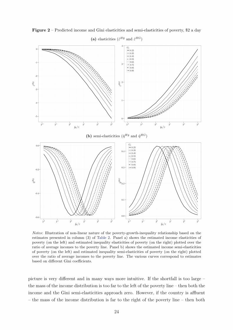
Figure 2 – Predicted income and Gini elasticities and semi-elasticities of poverty, $2 a day
(a) elasticities (εHy and εHG)
-5
-4
-3
-2
-1
0
2-2 2-1 20 21 22 23
yt/z
εHy
0
1
2
3
4
2-2 2-1 20 21 22 23
yt/z
εHG
Gt
0.25
0.35
0.45
0.55
0.65
0.75
0.85
0.95
(b) semi-elasticities (ηHy and ηHG)
-0.6
-0.4
-0.2
0.0
2-2 2-1 20 21 22 23
yt/z
ηH
y
0.0
0.1
0.2
0.3
0.4
2-2 2-1 20 21 22 23
yt/z
ηH
G
Gt
0.25
0.35
0.45
0.55
0.65
0.75
0.85
0.95
Notes: Illustration of non-linear nature of the poverty-growth-inequality relationship based on theestimates presented in column (3) of Table 2. Panel a) shows the estimated income elasticities ofpoverty (on the left) and estimated inequality elasticities of poverty (on the right) plotted over theratio of average incomes to the poverty line. Panel b) shows the estimated income semi-elasticitiesof poverty (on the left) and estimated inequality semi-elasticities of poverty (on the right) plottedover the ratio of average incomes to the poverty line. The various curves correspond to estimatesbased on different Gini coefficients.
picture is very different and in many ways more intuitive. If the shortfall is too large –
the mass of the income distribution is too far to the left of the poverty line – then both the
income and the Gini semi-elasticities approach zero. However, if the country is affluent
– the mass of the income distribution is far to the right of the poverty line – then both
24
semi-elasticities also approach zero. In between those two extremes, improvements in the
income distribution can make a very large difference in terms of percent of the population
lifted out of poverty, both directly through redistribution and indirectly through growth.
When mean income is at the poverty line (yt/z = 1), for example, a Gini of 0.25 implies
that one percent income growth leads to a 0.584 percentage point reduction in the poverty
headcount; and a Gini of 0.55 implies that one percent income growth leads to a 0.378
percentage point reduction in the poverty headcount. Especially at very low average
income levels the initial income distribution is decisive; it practically determines whether
there is potential for poverty alleviation through income growth at all (in terms of the
proportion of poor). Moreover, improvements in the income distribution will have a larger
poverty reducing effect at lower (initial) levels of inequality. Contrary to elasticities,
semi-elasticities suggest that poverty reduction strategies should focus both on income
growth and equalization, especially in low-income countries where the total returns to
redistribution are large. Again, for policy purposes, these relationships are much more
pertinent than relative changes in the poverty headcount.25
Could the decomposition be improved by allowing for other, ‘more ultimate’
determinants of poverty? If the assumption of log-normality is justified, mean income and
the Gini fully describe the distribution of incomes and expenditures, and there is no scope
for additional determinants. Yet log-normality is restrictive and we deliberately do not
rely on it; in fact, we expect it to be violated at least in some cases (see, e.g., the host of
alternative distributions analyzed by Bresson, 2009). More realistic distributions usually
have more than one shape parameter in order to better capture skewness, a long tail, or
the existence of multiple modes. ‘Ultimate factors’ could thus be proxies for systematic
deviations from equiproportional shifts in the distribution of incomes and expenditures.
Weak institutions, for example, might explain the fact that the rich capture more of the
gains of growth. Table B-4 in Appendix B extends the heteroskedastic fractional probit
models with data on institutions, human capital, access to credit and trade openness.
The APEs of income and inequality are not affected by the inclusion of the additional
covariates and the APEs of the latter are virtually zero. Thus we conclude that with
only two variables, some dummies and correlated random effects, these specifications
are essentially saturated. Contrary to linear approximations, the fractional response
approach leaves little room for underspecification of the decomposition.
While the literature on poverty reduction has produced mixed results so far, it is
largely consistent with this view. Prominent examples are two studies by Dollar and
Kraay (2002, 2004). These authors find that trade, inflation and other factors influence
the incomes of the poorest quintile, while several other variables do not. However, they
25This finding should stand with the new 2011 PPPs as well. Different PPPs would shift incomes,the poverty line and the poverty rates, and so countries would be located differently on the graph; butthe position of the curves in terms of relative incomes, yt/z, would be comparable.
25
emphasize that the effects run predominantly through growth of GDP per capita. The
relevant link is not between some factor X and a measure of poverty, but between X
and income or inequality; those are the relationships deserving a theoretical basis with
attention for causality issues. Thus if one is interested in the effects of, say, institutions
on poverty, our recommendation is to investigate the effects of institutions on income (cf.
Acemoglu et al., 2001) and inequality (cf. Easterly, 2007). Distinguishing this layer of
relationships is important, as the impacts of income and distributional changes themselves
depend on the initial levels of income and inequality.
5.3 Contributions
We now turn to the contributions of growth and redistribution to poverty reduction
since the early 1980s. We are going to show that there has been a marked shift in
the distributional pattern of growth towards pro-poor growth around the turn of the
millennium.
The contribution of growth or redistribution to poverty changes in some predefined
period is the product of their impact (partial effect, semi-elasticity) and their actual
variation, usually expressed as a proportion of the total change in the poverty rate over
the same period. Together with the stylized fact, illustrated in Figure B-4, that growth
tends to be distribution-neutral, the relative contributions of growth and redistribution
have been used to highlight the primacy of growth for poverty reduction (see e.g. Dollar
and Kraay, 2002; Kraay, 2006; Kraay et al., 2014; Dollar et al., 2016). Kraay (2006), for
example, concludes that long-run differences in poverty reduction can largely be explained
by growth in average incomes, as opposed to changes in inequality, which seem to matter
only in the short run. A good deal of the primacy of growth is due to the fact that there is
a lot more long-run variation in growth than in inequality. Even so, the poverty reducing
quality of growth is of legitimate concern. While the cross-country correlation between
growth and changes in inequality is near zero, this correlation varies across countries,
regions, and time periods (see also Ravallion and Chen, 2003). In fact, the variability of
the (semi-)elasticities emphasized above, together with the variability of average incomes
and inequality, can give rise to all sorts of relative contributions.
Some additional notation will prove useful. Following Datt and Ravallion (1992), a
discrete-time, non-logarithmic version of the decomposition of poverty changes is
∆Ht ≈[H(yt/z, Lt−1)−H(yt−1/z, Lt−1)
]+[H(yt−1/z, Lt)−H(yt−1/z, Lt−1)
](15)
where Lt is the Lorenz curve which, given micro-data, can be estimated non-
parametrically. The first brackets on the right-hand side contain the ‘growth component’,
the second the ‘distributional component’ of poverty reduction; we will refer to them as
Y and D respectively. Two of the four terms inside the brackets are unobservable:
26
H(yt/z, Lt−1) is the poverty rate when average income has evolved but the Lorenz curve
is kept unchanged; H(yt−1/z, Lt) is the poverty rate when the distribution has shifted but
average income is kept constant. The decomposition is approximate and ‘path dependent’,
generating a residual.26
In the present, cross-country context, the fractional response model estimated
above suggests a simple approach: we approximate H(yt/z, Lt) by our earlier function
H(yt/z,Gt), and replace the unknown quantities by predicted counterparts H(yt/z,Gt−1)
and H(yt−1/z,Gt).
Eq. (15) is deliberately written in absolute differences, even though the decomposition
is often carried out in relative terms (using logarithmic differences). This is in line
with the fractional response approach, where poverty levels are the natural metric. Two
other considerations motivate this choice. First, proportional decompositions are very
sensitive to levels approaching zero. Second, they overstate the growth component in
relatively rich regions and understate it in relatively poor regions, due to the mechanical
rise of the income elasticity over the development process. As a result, decompositions in
relative terms affect our ability to assess the contributions correctly and to detect poverty
convergence (Ravallion, 2012; Cuaresma et al., 2016).
It is interesting to carry out the decomposition over different time periods. We
construct three data sets for this purpose: one using the longest possible spells of surveys
of the same type between 1981 and 2010; and two for the sub-periods 1981-2000 and 2000-
2010. Since the availability of surveys before 2000 is more limited, the average spell length
in the two sub-periods is comparable: both have a mean and median duration between the
initial and final surveys of about seven years. The break point is not chosen by accident.
The turn of the millennium marked a qualitative change in the growth performance
of developing countries, who collectively grew faster than the developed world for the
subsequent decade. What we are interested in here is whether this development might
have coincided with a shift in the quality of growth.
We borrow from the growth accounting literature to define the shares of growth and
inequality (see e.g. Klenow and Rodriguez-Clare, 1997; Caselli, 2005). Table 5 shows
the results of a regional variance-covariance decomposition of all spells occurring within
a particular region and period using the $2.00 a day poverty line. Within each of
the three periods we compute the variance of the growth component, VAR(Y ), the
variance of the distribution component, VAR(D), and their covariance, COV(Y,D).
From these we obtain the cross-country share of the growth component as sY =
[VAR(Y ) + COV(Y,D)]/[VAR(Y ) + VAR(D) + 2COV(Y,D)], and the share of the
26To get rid of the path dependency we may average eq. (15) with a second decomposition swappingt and t − 1 in eq. (15); this delivers what Shorrocks (2013) calls the ‘Shapley decomposition’. In ourcase, the decomposition residual also includes prediction errors which should probably not be distributedacross the two input factors.
27
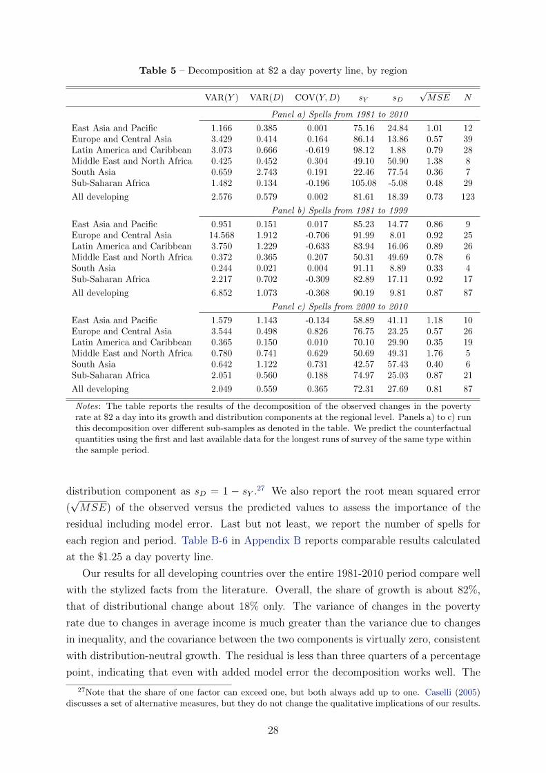
Table 5 – Decomposition at $2 a day poverty line, by region
VAR(Y ) VAR(D) COV(Y,D) sY sD√MSE N
Panel a) Spells from 1981 to 2010
East Asia and Pacific 1.166 0.385 0.001 75.16 24.84 1.01 12Europe and Central Asia 3.429 0.414 0.164 86.14 13.86 0.57 39Latin America and Caribbean 3.073 0.666 -0.619 98.12 1.88 0.79 28Middle East and North Africa 0.425 0.452 0.304 49.10 50.90 1.38 8South Asia 0.659 2.743 0.191 22.46 77.54 0.36 7Sub-Saharan Africa 1.482 0.134 -0.196 105.08 -5.08 0.48 29
All developing 2.576 0.579 0.002 81.61 18.39 0.73 123
Panel b) Spells from 1981 to 1999
East Asia and Pacific 0.951 0.151 0.017 85.23 14.77 0.86 9Europe and Central Asia 14.568 1.912 -0.706 91.99 8.01 0.92 25Latin America and Caribbean 3.750 1.229 -0.633 83.94 16.06 0.89 26Middle East and North Africa 0.372 0.365 0.207 50.31 49.69 0.78 6South Asia 0.244 0.021 0.004 91.11 8.89 0.33 4Sub-Saharan Africa 2.217 0.702 -0.309 82.89 17.11 0.92 17
All developing 6.852 1.073 -0.368 90.19 9.81 0.87 87
Panel c) Spells from 2000 to 2010
East Asia and Pacific 1.579 1.143 -0.134 58.89 41.11 1.18 10Europe and Central Asia 3.544 0.498 0.826 76.75 23.25 0.57 26Latin America and Caribbean 0.365 0.150 0.010 70.10 29.90 0.35 19Middle East and North Africa 0.780 0.741 0.629 50.69 49.31 1.76 5South Asia 0.642 1.122 0.731 42.57 57.43 0.40 6Sub-Saharan Africa 2.051 0.560 0.188 74.97 25.03 0.87 21
All developing 2.049 0.559 0.365 72.31 27.69 0.81 87
Notes: The table reports the results of the decomposition of the observed changes in the povertyrate at $2 a day into its growth and distribution components at the regional level. Panels a) to c) runthis decomposition over different sub-samples as denoted in the table. We predict the counterfactualquantities using the first and last available data for the longest runs of survey of the same type withinthe sample period.
distribution component as sD = 1 − sY .27 We also report the root mean squared error
(√MSE) of the observed versus the predicted values to assess the importance of the
residual including model error. Last but not least, we report the number of spells for
each region and period. Table B-6 in Appendix B reports comparable results calculated
at the $1.25 a day poverty line.
Our results for all developing countries over the entire 1981-2010 period compare well
with the stylized facts from the literature. Overall, the share of growth is about 82%,
that of distributional change about 18% only. The variance of changes in the poverty
rate due to changes in average income is much greater than the variance due to changes
in inequality, and the covariance between the two components is virtually zero, consistent
with distribution-neutral growth. The residual is less than three quarters of a percentage
point, indicating that even with added model error the decomposition works well. The
27Note that the share of one factor can exceed one, but both always add up to one. Caselli (2005)discusses a set of alternative measures, but they do not change the qualitative implications of our results.
28
results for the $1.25 a day poverty line (Table B-6) are qualitatively similar and broadly
match those reported in Kraay (2006).
The breakdown of the results by region also tells a familiar story. Growth dominated
poverty reduction in Sub-Saharan Africa (where incomes first declined, then stagnated
and then recovered again), in Latin America (where inequality was persistently high
for most of the period in question), and in Europe and Central Asia (where the
post-communist transition was accompanied by rapid movements in average incomes).
Distributional change played a larger role in East Asia and Pacific, Middle East and
North Africa, and South Asia, where it was responsible for about one, two and three
quarters of the poverty evolution, respectively. Some of these results come with a caveat,
though. In South Asia, although we have all but one countries represented, the sample
size is very small.28 In the Middle East and North Africa, survey coverage is notoriously
bad, we have less than half of all countries in the sample, and the residual is more than
twice the average.
So what’s new? A very different picture emerges once we split the sample at the
turn of the millennium. The corresponding results are reported in Panel b) and Panel
c) of Table 5. Growth was responsible for nearly all of the changes in the poverty rate
before 2000, but its share fell to 72% in the following decade. Since the mean spell
lengths are about the same, this is not due to a long run vs. short run difference.
Instead, this development seems to be the result of a shift in the poverty reducing quality
of growth. Panel b) shows that before 2000 the correlation between the growth and
distribution component was negative for all developing countries as a whole and for half
of the regions. Panel c) demonstrates that after 2000 the correlation between the two
components turned positive for the sample as a whole and in all regions apart from East
Asia. Positive growth coincided with reductions in inequality more often. Table B-6 in
Appendix B confirms that this pattern also holds at the $1.25 a day poverty line.
Figure 3 helps to make this point more tangible. The upper panel shows how the
correlation between the estimated growth and distribution components changed over the
turn of the millennium. Before 2000, reductions in poverty through growth often coincided
with adverse distributional change (the lower right quadrant), while negative economic
growth often coincided with pro-poor distributional change (the upper left quadrant).
Since 2000, the situation is very different. In the great majority of cases, poverty reduction
through growth was aided by pro-poor distributional change (the lower left quadrant).
In fact, only in a few cases, distributional change did not occur in tandem with growth
(the lower right quadrant). Growth itself only contributed to rising poverty in a handful
of cases (both upper quadrants). The lower panel also shows that our estimated growth
components closely track the observed change in the poverty rate in both samples. Here
28The large share of the distribution component is driven by the Maldives and Bhutan, where nearlyall or about half of poverty reduction can be attributed to changes in distribution.
29
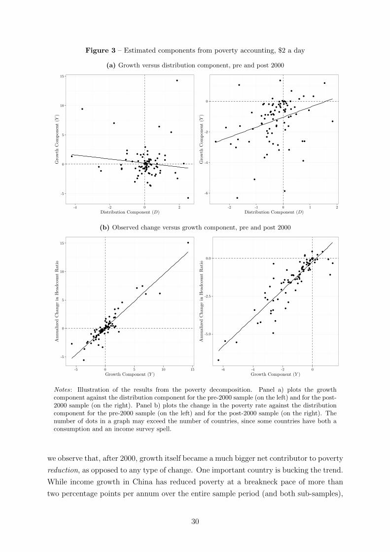
Figure 3 – Estimated components from poverty accounting, $2 a day
(a) Growth versus distribution component, pre and post 2000
-5
0
5
10
15
-4 -2 0 2
Distribution Component (D)
Growth
Com
ponent(Y
)
-6
-4
-2
0
-2 -1 0 1 2
Distribution Component (D)
Growth
Com
ponent(Y
)
(b) Observed change versus growth component, pre and post 2000
-5
0
5
10
15
-5 0 5 10 15
Growth Component (Y )
Annualized
Chan
gein
HeadcountRatio
-5.0
-2.5
0.0
-6 -4 -2 0
Growth Component (Y )
Annualized
Change
inHeadcountRatio
Notes: Illustration of the results from the poverty decomposition. Panel a) plots the growthcomponent against the distribution component for the pre-2000 sample (on the left) and for the post-2000 sample (on the right). Panel b) plots the change in the poverty rate against the distributioncomponent for the pre-2000 sample (on the left) and for the post-2000 sample (on the right). Thenumber of dots in a graph may exceed the number of countries, since some countries have both aconsumption and an income survey spell.
we observe that, after 2000, growth itself became a much bigger net contributor to poverty
reduction, as opposed to any type of change. One important country is bucking the trend.
While income growth in China has reduced poverty at a breakneck pace of more than
two percentage points per annum over the entire sample period (and both sub-samples),
30
rising inequality has worked in the opposite direction. China’s share of world poverty is
falling rapidly, but this trend may pose challenges of its own farther down the road.
Overall, our interpretation of these results challenges the conventional wisdom
that growth is distribution-neutral. The evidence suggests that growth has become
substantially more pro-poor since the turn of the millennium, in two ways: (i) in the
relative sense, that is, it benefits the poor disproportionately, and (ii) in the absolute
sense, that is, it reduces poverty more often than not. If this trend can be maintained
this is good news for the goal of ending absolute poverty within a few decades.
5.4 Projections
So what can we say about the prospects of poverty reduction? In 2015, all member states
of the United Nations agreed to ‘eradicate extreme poverty for all people everywhere,
currently measured as people living on less than $1.25 a day’ by 2030. The key question
we ask now is whether this new goal is attainable, or if the global goalpost has been set
so high, that it may fail to promote a sensible allocation of development assistance.
We begin with comparing the in-sample predictions of our model for 2010 to the
official World Bank data to show that they match up well. Then, we extrapolate poverty
until 2030. Clearly, this is a hypothetical exercise and is not intended to replace any
official estimates by the World Bank or national authorities. Rather, it allows us to make
somewhat more sophisticated predictions than back-of-the-envelope trend extrapolations
and can provide a useful benchmark for setting global poverty reduction goals. Using our
models for this purpose has the added advantage that we can predict poverty responses
to any combination of shifts in mean income and inequality.
The official World Bank regional poverty figures involve a considerable amount
of interpolation and extrapolation, since most household surveys are not undertaken
annually (for details see Chen and Ravallion, 2004). The basic steps are as follows. Lorenz
curves are fitted to either unit-level or group-level data in the actual survey years. Next,
average real household incomes are lined up to a reference year by interpolating between
surveys or extrapolating with the growth rate of personal consumption expenditures per
capita (PCEit). The poverty headcount for the reference year is then calculated using the
new income level and the Lorenz curve from the nearest earlier year; or, if two surveys are
available, one before and one after the reference year, the poverty headcount is calculated
with both Lorenz curves and then averaged.
Our method is similar in spirit. It involves four steps. First, we extrapolate the
last available survey income to 2010 using actually observed country growth rates in
PCEit from the national accounts.29 Second, we project mean income into the future,
29The term ‘national accounts’ refers to data from the World Development Indicators or the PennWorld Table 7.1, whichever has more data over the 30 year horizon.
31
using one of three constant-growth scenarios and one of three distributional scenarios.
Third, we predict each country’s poverty rate in 5-year intervals from 2010 to 2030 using
the estimates from column (2) in Table 2.30 We may neglect measurement errors in
income or inequality for forecasting purposes, implicitly assuming that their influence
remains stable over time. Fourth and finally, regional aggregates and the world total are
calculated as population-weighted averages of the country estimates, using World Bank
population projections. No standard errors are provided for the projections in view of
the fundamental uncertainty in the assumed growth rates and distributional patterns of
growth.
We base our three different constant-growth scenarios on the historical PCEit growth
rates from the national accounts in three predefined periods. An ‘optimistic’ scenario uses
the average PCEit growth rate of each country over 2000-2010, a decade characterized
by fast growth. A ‘moderate’ growth scenario uses the average PCEit growth rate of
each country from 1980 to 2010 – the long run average over the entire sample period.
Finally, a ‘pessimistic’ growth scenario uses the 1980-2000 growth rates. The latter
scenario is hopefully unlikely; it implies that mean consumption in Sub-Saharan Africa,
in particular, is shrinking at a rate of about 0.82% per year.31 Table B-3 in the appendix
reports population-weighted regional growth rates over these periods to illustrate the
implied regional income dynamics.32
For each growth scenario, we also simulate three different inequality patterns. ‘Pro-
poor growth’ implies an annual decline in the Gini coefficient of approximately -0.5%;
‘distribution-neutral growth’ keeps inequality constant at the level prevailing in 2010, in
line with the observed zero correlation between changes in inequality and income growth
over the entire sample; and ‘pro-rich growth’ implies an annual increase in the Gini
coefficient of approximately 0.5%. For illustration consider the following example. If a
country’s Gini coefficient is 0.40 in 2010 and we apply the pro-poor pattern, then by 2030
we project a Gini coefficient of about 0.36; if we apply the pro-rich pattern, then the
Gini coefficient is about 0.44 in 2030. Changes of this magnitude are in line with the
population-weighted regional trends obtained from the surveys.
Our in-sample estimates for 2010 compare well with the ‘official’ World Bank figures.
We can almost perfectly match the World Bank’s results for the world total. We estimate
a poverty rate of 40.37% in 2010 at the $2 a day poverty line, whereas the World Bank
reports 40.67%.33 Using the same population data, our estimates imply about 2.378
30Although this specification is only estimated on the sub-sample where Ti ≥ 2, we can use theestimates to predict poverty for the entire sample (Ti ≥ 1). We only lack estimates of the panel sizeeffects for Ti = 1, so we assign these observations to the adjacent group (Ti = 2).
31Owing to the post-communist transition, consumption and incomes in Europe and Central Asiawere shrinking over the same period. However, given the small number of poor in 2010, the influence ofthat region on the global poverty headcount in 2030 is minimal.
32All reported growth rates are computed as log-differences unless noted otherwise.33This was the official number until the Oct. 9, 2014 update of PovcalNet.
32
billion people under the $2 line versus 2.395 billion as reported by the World Bank. For
three regions, our estimates are within one percentage point of the official figures; for the
other three, they are within 3 percentage points.34 The performance of our predictions
at the $1.25 a day line is comparable. We estimate a poverty rate of 20.41% in 2010 and
the World Bank reports 20.63%. In absolute numbers, this means that about 1.2 billion
people on the planet were extremely poor in 2010. Note that in 2010 the composition of
countries (or people) near the $2 a day poverty line is reminiscent of its $1.25 counterpart
in the early 2000s. Fast growing East Asia and moderately fast growing South Asia still
make up more than half of global poverty, implying that progress in these two regions
will have a large effect on the overall poverty headcount.
Table 6 shows our projections for 2030 under the $2 poverty line. Our moderate
growth scenario predicts that about 1.87 billion people (26%) live on less than $2 a day
in 2030, vs. 2.4 billion (40.37%) in 2010. However, much greater gains are possible.
Global poverty under the $2 line falls by half to less than 20% of the developing world’s
population in the optimistic growth scenario with distribution-neutral or pro-poor growth.
If this happens by 2030, then more than one billion people will have left poverty at the
$2 line – undeniably a remarkable achievement.
Examining the regional distribution, we find that $2 poverty in East Asia is likely
to fall to around 5% by 2030, down from 29.7% in 2010. Nearly everyone in East Asia
will have entered the middle class by developing country standards. This forecast largely
hinges on fast growth in China.35 Progress in South Asia is also likely to be rapid.
According to our moderate growth estimate the expected poverty rate is 35.9% in 2030,
meaning about 716 million poor, down from 66.7% or 1.1 billion poor in 2010. In the
optimistic pro-poor growth case, the headcount ratio falls further to less than 20% and
the number of poor to less than 400 million. In stark contrast, the $2 a day poverty
rate in Sub-Saharan Africa is expected to remain very high. Our moderate growth
scenario predicts a poverty rate of about 66%, down from 69.9% in 2010, which at current
population projections implies almost one billion poor in Sub-Saharan Africa alone. Even
in the optimistic and pro-poor growth scenario, we project a poverty rate of over 50%
and more than 700 million poor. The bulk of the consumption distribution is too far to
the left of the $2 a day poverty line in 2010 for most of the subcontinent. Hence, poverty
alleviation in Sub-Saharan Africa remains the primary development challenge of the first
half of the 21st century.
These observations can in part be explained by a process of ‘bunching up above $1.25
34For Sub-Saharan Africa, for instance, we estimate a poverty rate of 69.36% and the World Bankreports 69.87%. For East Asia, we estimate 26.78%, whereas the World Bank figure is 29.73%.
35However, some observers suggest that China runs a non-negligible risk of falling into a ‘middle-income trap’ (Eichengreen, Park, and Shin, 2013) which might make East Asian poverty stick around10%. Our estimates suggest that this would require a very severe slowdown. For poverty in East Asiato remain above 10% at $2 a day, growth needs to be less than half of the 2000-2010 trend.
33
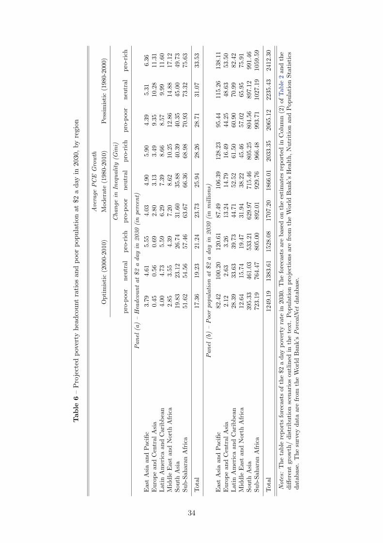
Table
6–
Pro
ject
edp
over
tyh
ead
cou
nt
rati
osan
dp
oor
pop
ula
tion
at$2
ad
ayin
2030
,by
regi
on
Ave
rage
PC
EG
row
th
Op
tim
isti
c(2
000-2
010)
Mod
erate
(1980-2
010)
Pes
sim
isti
c(1
980-2
000)
Chan
gein
Ineq
uali
ty(G
ini)
pro
-poor
neu
tral
pro
-ric
hp
ro-p
oor
neu
tral
pro
-ric
hp
ro-p
oor
neu
tral
pro
-ric
h
Pan
el(a
)–
Hea
dco
un
tat$2
aday
in2030
(in
perc
ent)
Eas
tA
sia
and
Pac
ific
3.7
94.6
15.5
54.0
34.9
05.9
04.3
95.3
16.3
6E
uro
pe
and
Cen
tral
Asi
a0.4
50.5
60.6
92.8
03.1
33.4
99.3
510.2
811.3
1L
atin
Am
eric
aan
dC
arib
bea
n4.0
04.7
35.5
96.2
97.3
98.6
68.5
79.9
911.6
0M
idd
leE
ast
and
Nor
thA
fric
a2.8
53.5
54.3
97.2
08.6
210.2
512.8
614.8
817.1
2S
outh
Asi
a19.8
323.1
226.7
431.6
035.8
840.3
940.3
545.0
049.7
3S
ub
-Sah
aran
Afr
ica
51.6
254.5
657.4
663.6
766.3
668.9
870.9
373.3
275.6
3
Tot
al17.3
619.2
321.2
423.7
325.9
428.2
628.7
131.0
733.5
3
Pan
el(b
)–
Poo
rpo
pu
lati
on
at$2
aday
in2030
(in
mil
lion
s)
Eas
tA
sia
and
Pac
ific
82.4
2100.2
0120.6
187.4
9106.3
9128.2
395.4
4115.2
6138.1
1E
uro
pe
and
Cen
tral
Asi
a2.1
22.6
33.2
613.2
414.7
916.4
944.2
548.6
353.5
0L
atin
Am
eric
aan
dC
arib
bea
n28.3
933.6
339.7
344.7
152.5
261.5
060.9
070.9
982.4
2M
idd
leE
ast
and
Nor
thA
fric
a12.6
415.7
419.4
731.9
438.2
245.4
657.0
265.9
575.9
1S
outh
Asi
a395.3
3461.0
3533.2
1629.9
7715.4
6805.2
5804.5
6897.1
2991.4
6S
ub
-Sah
aran
Afr
ica
723.1
9764.4
7805.0
0892.0
1929.7
6966.4
8993.7
11027.1
91059.5
9
Tot
al1249.1
91383.6
11528.0
81707.2
01866.0
12033.3
52065.1
22235.4
32412.3
0
Note
s:T
he
tab
lere
por
tsfo
reca
sts
ofth
e$2
ad
ayp
over
tyra
tein
2030.
Th
efo
reca
sts
are
base
don
the
esti
mate
sre
port
edin
Colu
mn
(2)
of
Tab
le2
an
dth
ed
iffer
ent
grow
th/
dis
trib
uti
onsc
enar
ios
outl
ined
inth
ete
xt.
Pop
ula
tion
pro
ject
ion
sare
from
the
Worl
dB
an
k’s
Hea
lth
,N
utr
itio
nan
dP
op
ula
tion
Sta
tist
ics
dat
abas
e.T
he
surv
eyd
ata
are
from
the
Wor
ldB
ank’s
Povc
alN
etd
ata
base
.
34
a day and just below $2 a day’ occurring in East Asia and, to a lesser extent, in South
Asia over the last two decades (Chen and Ravallion, 2010). These two regions have a
relatively large population near the poverty line and hence most of the advances are
projected to occur there. Latin America and the Caribbean, as well as the Middle East
and North Africa, are richer and require stronger income growth to continuously reduce
poverty. Sub-Saharan Africa, on the other hand, has a considerable proportion of poor
far below the $2 a day line in 2010 (with almost half the population below $1.25 a day).
It is facing a lower income elasticity and an income semi-elasticity that is below its peak.
Hence, the subcontinent needs exceptionally strong income growth to make significant
strides against poverty.
We repeat this exercise using the $1.25 a day poverty line. Table B-7 in Appendix B
shows the results based on the estimates of Table B-5. Under moderate growth we project
a global poverty rate of 13.2% in 2030, meaning about 950 million extremely poor people
versus 1.2 billion in 2010. The pace of poverty reduction will have slowed significantly
both in terms of relative changes and in terms of numbers of poor people. About 70% of
the world’s poor will live in Sub-Saharan Africa and about 23% in South Asia by 2030.
Under optimistic, distribution-neutral growth, we find a global poverty rate of 9.11% in
2030, with about 655 million people remaining extremely poor. About 76% of those live
in Sub-Saharan Africa and about 17% in South Asia. Under a pessimistic, distribution-
neutral growth scenario, there is almost no progress at all. The global poverty headcount
is estimated at 16.82% and the world is still home to 1.2 billion extremely poor people.
What do these results imply for the post-2015 development agenda? In a nutshell,
2030 is unlikely to mark the end of extreme poverty, even under very optimistic
assumptions. Figure 4 plots the historical evolution of world poverty from 1981 to 2010,
a trend fitted through the observed data and extrapolated until 2030, and our different
scenarios. The linear trend serves as a reference for the non-linear projections. The
distribution-neutral scenarios are the solid lines, with the moderate growth case in solid
black and the other two cases in gray. The dotted lines are the pro-rich and pro-poor
cases. The left panel shows the results at the $1.25 a day poverty line, the right panel at
the $2 a day poverty line.
Several points are worth noting. First, only the linear extrapolation predicts an
extreme poverty rate in the vicinity of zero by 2030. Regressing the global $1.25 a day
poverty rate on time yields a downward slope of about one percentage point per year (as
in Ravallion, 2013). Starting from a global poverty rate of 20.6% in 2010, the linear trend
predicts that extreme poverty will be vanquished around 2030. Second, at the $1.25 a
day line, all projections show a decelerating trend in of poverty reduction. Even in the
optimistic scenarios, the pace of poverty reduction slows down, though the slowdown
becomes noticeable later. Third, most scenarios suggest a $1.25 poverty rate higher
than 10% in 2030; the optimistic pro-poor and distribution-neutral scenarios project
35
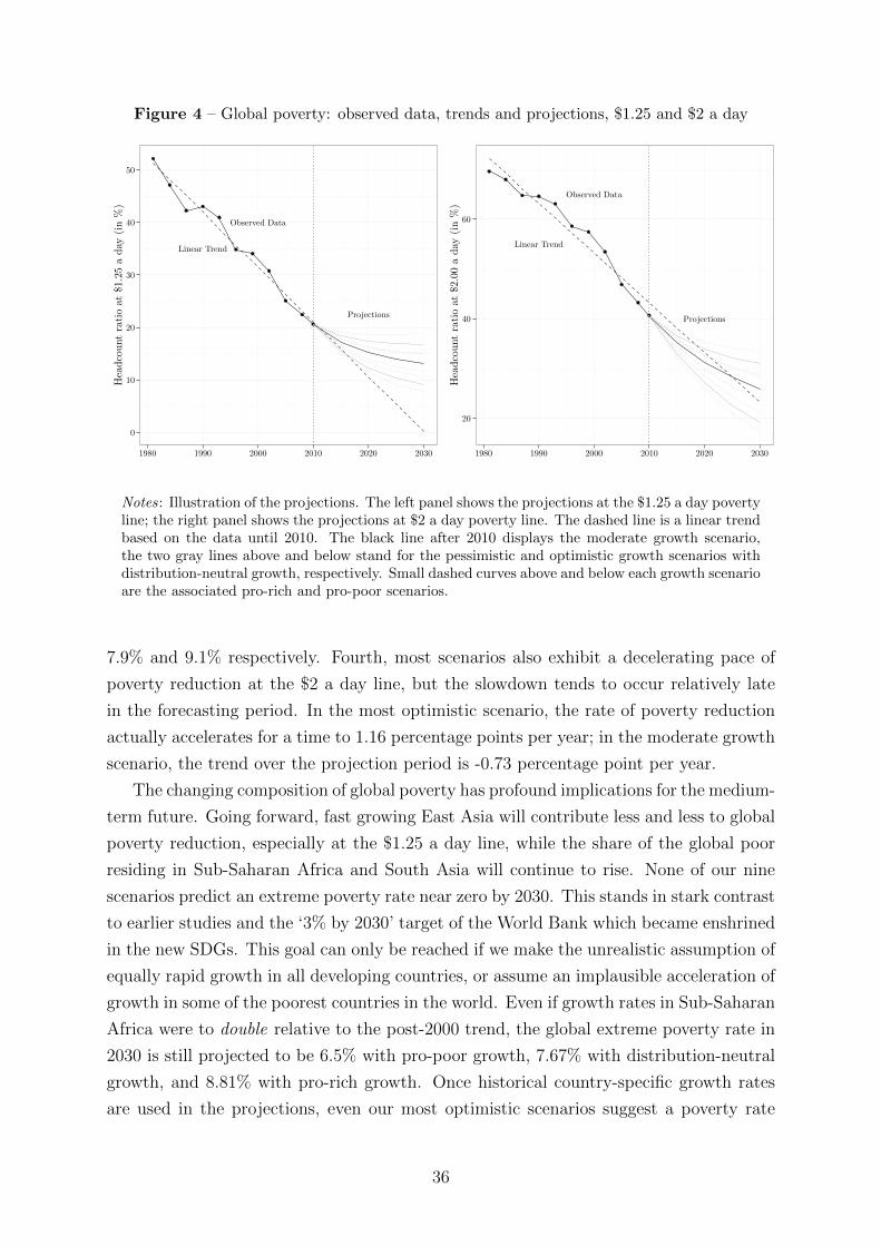
Figure 4 – Global poverty: observed data, trends and projections, $1.25 and $2 a day
Observed Data
Linear Trend
Projections
0
10
20
30
40
50
1980 1990 2000 2010 2020 2030
Headcountratioat
$1.25aday
(in%)
Observed Data
Linear Trend
Projections
20
40
60
1980 1990 2000 2010 2020 2030Headcountratioat$2.00aday
(in%)
Notes: Illustration of the projections. The left panel shows the projections at the $1.25 a day povertyline; the right panel shows the projections at $2 a day poverty line. The dashed line is a linear trendbased on the data until 2010. The black line after 2010 displays the moderate growth scenario,the two gray lines above and below stand for the pessimistic and optimistic growth scenarios withdistribution-neutral growth, respectively. Small dashed curves above and below each growth scenarioare the associated pro-rich and pro-poor scenarios.
7.9% and 9.1% respectively. Fourth, most scenarios also exhibit a decelerating pace of
poverty reduction at the $2 a day line, but the slowdown tends to occur relatively late
in the forecasting period. In the most optimistic scenario, the rate of poverty reduction
actually accelerates for a time to 1.16 percentage points per year; in the moderate growth
scenario, the trend over the projection period is -0.73 percentage point per year.
The changing composition of global poverty has profound implications for the medium-
term future. Going forward, fast growing East Asia will contribute less and less to global
poverty reduction, especially at the $1.25 a day line, while the share of the global poor
residing in Sub-Saharan Africa and South Asia will continue to rise. None of our nine
scenarios predict an extreme poverty rate near zero by 2030. This stands in stark contrast
to earlier studies and the ‘3% by 2030’ target of the World Bank which became enshrined
in the new SDGs. This goal can only be reached if we make the unrealistic assumption of
equally rapid growth in all developing countries, or assume an implausible acceleration of
growth in some of the poorest countries in the world. Even if growth rates in Sub-Saharan
Africa were to double relative to the post-2000 trend, the global extreme poverty rate in
2030 is still projected to be 6.5% with pro-poor growth, 7.67% with distribution-neutral
growth, and 8.81% with pro-rich growth. Once historical country-specific growth rates
are used in the projections, even our most optimistic scenarios suggest a poverty rate
36
of between 7.9% and 10.5%, depending on the evolution of inequality. However, at $2
a day, the slowdown will occur much later and bigger gains are possible, mirroring the
achievements of the last two decades.
Two caveats are in order when it comes to comparing our estimates to recent figures
from the World Bank. First, the World Bank switched from reporting global poverty
in percent of the developing world population to percent of the global population.
This shaves a few percentage points off their estimates and makes the goal seem more
attainable. Second, although the recently released 2011 PPPs suggest that the poorest
regions are a little less poor and middle-income regions a little poorer, the global poverty
rate in 2010 only changed by about one tenth of a percentage point. This is a trivial
difference in comparison with the fundamental uncertainties involved in estimating such
a global number.36
6 Concluding remarks
The impact of income growth and changes in inequality on poverty, and their contribution
to poverty reduction, have attracted considerable attention among policy makers and the
academic literature in recent decades. In this paper we develop a new approach to
estimating these quantities within a unified poverty accounting framework, apply this
approach to a large cross-country data set, and show that it generates interesting and
new findings. Our starting point is that the well-established non-linearity of the income
and inequality elasticities of poverty arises primarily from the bounded nature of the
poverty headcount ratio. Once this inherent non-linearity is taken into account, we can
derive an empirical approximation of the poverty decomposition that implies income and
inequality (semi-)elasticities with desirable properties.
We use our approach to estimate income and inequality (semi-)elasticities of poverty
based on a large new data set of 809 surveys from 124 developing countries over the
period 1981-2010. Our model fits the data extremely well. We provide evidence that
the average income elasticity is around minus two and the average inequality elasticity
is about one and a half. However, since these two averages are not very informative, we
show that differences in income and inequality levels create strong regional heterogeneity
in the estimated elasticities and semi-elasticities. We also highlight that the semi-
elasticities which we argue policy makers should care about are distinctly non-linear.
Studies based on linear approximations do not capture this heterogeneity and non-
linearity. Compared to earlier results, our approach provides estimates that are often
substantially different, very stable and considerably more accurate. This holds for a wide
range of different combinations of income and inequality. While we restrict the nature
36See Ravallion (2016) for an up-to-date discussion of these challenges.
37
of the unobserved heterogeneity (measurement differences), we require no distributional
assumptions other than a correctly specified conditional mean. In other words, our models
closely approximate the shape of the Lorenz curve near the poverty line using only two
summary measures of the distribution: the mean and the Gini coefficient.
Another advantage of the proposed approach is that it allows us to recover the
conditional expectation of the poverty rate. We use this property to predict the
counterfactual terms needed to identify the historical contribution of income growth
and distributional change on poverty reduction. We then show that growth was chiefly
responsible for poverty reduction in the pre-2000 period, but that changes in inequality
play a much larger role since the turn of the millennium. Hence, inequality matters, not
just in the short run.
To further illustrate the usefulness of our framework, we project global and regional
poverty rates from 2010 until 2030 based on several scenarios about how historical
consumption growth and patterns of inequality extend into the medium-term future.
We show that the regional landscape of poverty is likely to change dramatically over
the next two decades. Two findings stand out in particular. First, with strong growth
and moderate pro-poor distributional change another billion people may be lifted out of
poverty at the $2 a day poverty line. Second, poverty reduction at the $1.25 a day poverty
line is likely to slow down towards the end of the projection period. As a result, the goal
of ending extreme poverty within a generation is unlikely to be achieved. Our optimistic
forecasts hinge on very favorable assumptions about the future growth trajectories of
some of the world’s poorest economies. This, coupled with strong expected population
growth in those countries, implies that at least half a billion people are still likely to be
extremely poor by 2030.
Our results should not be very sensitive to the use of 2005 rather than the recently
released 2011 PPPs, provided we shift the international poverty line accordingly to $1.90
or $2.65 a day. Although the relative incomes of some regions changed with the new 2011
PPPs and price levels in many developing countries were revised downwards, the new
poverty lines were re-drawn with the explicit aim of keeping the global yardstick constant
(see Ferreira et al., 2015).
Finally, it may be tempting to interpret some of our findings as confirming the primacy
of growth. Yet, we are promoting a rather different view. There is a potentially large
‘double dividend’ to be reaped if growth can be achieved in combination with simultaneous
reductions in inequality. It is also important to emphasize that the causal effect of
any particular policy on aggregate household income and the relative distribution of
income cannot be discerned from a decomposition exercise such as ours. Hence, the
importance of institutions, trade and a host of other factors for poverty alleviation remains
undiminished. What we do identify is how a given change in average incomes or the
distribution of incomes translates into poverty outcomes.
38
References
Aaron, H. (1967). The foundations of the “war on poverty” reexamined. American EconomicReview 57 (5), 1229–1240.
Acemoglu, D., S. Johnson, and J. A. Robinson (2001). The colonial origins of comparative development:An empirical investigation. American Economic Review 91 (5), 1369–1401.
Adams, R. H. (2004). Economic growth, inequality and poverty: Estimating the growth elasticity ofpoverty. World Development 32 (12), 1989–2014.
Altonji, J. G. and R. L. Matzkin (2005). Cross section and panel data estimators for nonseparable modelswith endogenous regressors. Econometrica 73 (4), 1053–1102.
Barro, R. J. and J. W. Lee (2013). A new data set of educational attainment in the world, 1950–2010.Journal of Development Economics 104, 184–198.
Battistin, E., R. Blundell, and A. Lewbel (2009). Why is consumption more log normal than income?Gibrat’s law revisited. Journal of Political Economy 117 (6), 1140–1154.
Beck, T., A. Demirguc-Kunt, and R. Levine (2010). Financial institutions and markets across countriesand over time: The updated financial development and structure database. World Bank EconomicReview 24 (1), 77–92.
Besley, T. and R. Burgess (2003). Halving global poverty. Journal of Economic Perspectives 17 (3), 3–22.
Blundell, R. W. and J. L. Powell (2004). Endogeneity in semiparametric binary response models. Reviewof Economic Studies 71 (3), 655–679.
Bourguignon, F. (2003). The growth elasticity of poverty reduction: Explaining heterogeneity acrosscountries and time periods. In T. S. Eicher and S. J. Turnovsky (Eds.), Inequality and Growth:Theory and Policy Implications, pp. 3–26. Cambridge, MA: MIT Press.
Bresson, F. (2009). On the estimation of growth and inequality elasticities of poverty with grouped data.Review of Income and Wealth 55 (2), 266–302.
Caselli, F. (2005). Accounting for cross-country income differences. Volume 1, Part A of Handbook ofEconomic Growth, Chapter 9, pp. 679–741. Elsevier.
Chamberlain, G. (1984). Panel data. Volume 2 of Handbook of Econometrics, pp. 1247–1318. Elsevier.
Chambers, D. and S. Dhongde (2011). A non-parametric measure of poverty elasticity. Review of Incomeand Wealth 57 (4), 683–703.
Chen, S. and M. Ravallion (2004). How have the world’s poorest fared since the early 1980s? The WorldBank Research Observer 19 (2), 141–169.
Chen, S. and M. Ravallion (2010). The developing world is poorer than we thought, but no less successfulin the fight against poverty. Quarterly Journal of Economics 125 (4), 1577–1625.
Chesher, A. and C. Schluter (2002). Welfare measurement and measurement error. Review of EconomicStudies 69 (2), 357–378.
Chotikapanich, D., W. E. Griffiths, and D. S. P. Rao (2007). Estimating and combining national incomedistributions using limited data. Journal of Business & Economic Statistics 25 (1), 97–109.
Cuaresma, J. C., S. Klasen, and K. M. Wacker (2016). There is poverty convergence. Technical report,Vienna University of Economics and Business, Department of Economics.
Datt, G. and M. Ravallion (1992). Growth and redistribution components of changes in povertymeasures: A decomposition with applications to Brazil and India in the 1980s. Journal of DevelopmentEconomics 38 (2), 275–295.
Deaton, A. and A. Heston (2010). Understanding PPPs and PPP-based national accounts. AmericanEconomic Journal: Macroeconomics 2 (4), 1–35.
Dollar, D., T. Kleineberg, and A. Kraay (2016). Growth still is good for the poor. European EconomicReview 81, 68–85.
Dollar, D. and A. Kraay (2002). Growth is good for the poor. Journal of Economic Growth 7 (3),195–225.
Dollar, D. and A. Kraay (2004). Trade, growth, and poverty. Economic Journal 114 (493), F22–F49.
Easterly, W. (2007). Inequality does cause underdevelopment: Insights from a new instrument. Journalof Development Economics 84 (2), 755–776.
Eichengreen, B., D. Park, and K. Shin (2013, January). Growth slowdowns redux: New evidence on themiddle-income trap. Working Paper 18673, National Bureau of Economic Research.
Ferreira, F. H., S. Chen, Y. Dikhanov, N. Hamadeh, D. Jolliffe, A. Narayan, E. B. Prydz, A. Revenga,P. Sangraula, U. Serajuddin, and N. Yoshida (2015, October). A global count of the extreme poor in
39
2012: data issues, methodology and initial results. Policy Research Working Paper 7432, The WorldBank.
Gourieroux, C., A. Monfort, and A. Trognon (1984). Pseudo maximum likelihood methods: Theory.Econometrica 52 (3), 681–700.
Hausman, J. A. (1978). Specification tests in econometrics. Econometrica 46 (6), 1251–1271.
Hoover, G. A., W. Enders, and D. G. Freeman (2008). Non-white poverty and macroeconomy: Theimpact of growth. American Economic Review 98 (2), 398–402.
Kakwani, N. (1993). Poverty and economic growth with application to Cote d’Ivoire. Review of Incomeand Wealth 39 (2), 121–139.
Kalwij, A. and A. Verschoor (2007). Not by growth alone: The role of the distribution of income inregional diversity in poverty reduction. European Economic Review 51 (4), 805–829.
Klasen, S. and M. Misselhorn (2008). Determinants of the growth semi-elasticity of poverty reduction.Working paper, Ibero America Institute for Economic Research.
Klenow, P. and A. Rodriguez-Clare (1997). The neoclassical revival in growth economics: Has it gone toofar? In B. S. Bernanke and J. J. Rotemberg (Eds.), NBER Macroeconomics Annual 1997, Volume 12,pp. 73–103. Cambridge, MA: MIT Press.
Kraay, A. (2006). When is growth pro-poor? Evidence from a panel of countries. Journal of DevelopmentEconomics 80 (1), 198–227.
Kraay, A., T. Kleineberg, and D. Dollar (2014). Growth, inequality, and social welfare: Cross-countryevidence. Working paper, Centre for Economic Policy Research.
Krause, M. (2014). Parametric lorenz curves and the modality of the income density function. Reviewof Income and Wealth 60 (4), 905–929.
Loudermilk, M. S. (2007). Estimation of fractional dependent variables in dynamic panel data modelswith an application to firm dividend policy. Journal of Business & Economic Statistics 25 (4), 462–472.
MacCullagh, P. and J. A. Nelder (1989). Generalized linear models (2nd ed.). Chapman & Hall/ CRCPress.
Milanovic, B. (2002). True world income distribution, 1988 and 1993: First calculation based onhousehold surveys alone. Economic Journal 112 (476), 51–92.
Mundlak, Y. (1978). On the pooling of time series and cross section data. Econometrica 46 (1), 69–85.
Neyman, J. and E. L. Scott (1948). Consistent estimates based on partially consistent observations.Econometrica 16 (1), 1–32.
Papke, L. E. and J. M. Wooldridge (1996). Econometric methods for fractional response variables withan application to 401(k) plan participation rates. Journal of Applied Econometrics 11 (6), 619–632.
Papke, L. E. and J. M. Wooldridge (2008). Panel data methods for fractional response variables with anapplication to test pass rates. Journal of Econometrics 145 (1–2), 121–133.
Ramalho, E. A., J. J. Ramalho, and J. M. Murteira (2011). Alternative estimating and testing empiricalstrategies for fractional regression models. Journal of Economic Surveys 25 (1), 19–68.
Ravallion, M. (2001). Growth, inequality and poverty: Looking beyond averages. WorldDevelopment 29 (11), 1803–1815.
Ravallion, M. (2012). Why don’t we see poverty convergence? American Economic Review 102 (1),504–523.
Ravallion, M. (2013). How long will it take to lift one billion people out of poverty? World Bank ResearchObserver 28 (2), 139–158.
Ravallion, M. (2016). Toward better global poverty measures. Journal of Economic Inequality 14 (2),227–248.
Ravallion, M. and S. Chen (1997). What can new survey data tell us about recent changes in distributionand poverty? World Bank Economic Review 11 (2), 357–382.
Ravallion, M. and S. Chen (2003). Measuring pro-poor growth. Economics Letters 78 (1), 93–99.
Rivers, D. and Q. H. Vuong (1988). Limited information estimators and exogeneity tests for simultaneousprobit models. Journal of Econometrics 39 (3), 347–366.
Sachs, J. D. and A. Warner (1995). Economic reform and the process of global integration. BrookingsPapers on Economic Activity 1995 (1), 1–118.
Sala-i-Martin, X. (2006). The world distribution of income: Falling poverty and . . . convergence, period.Quarterly Journal of Economics 121 (2), 351–397.
Santos Silva, J. and S. Tenreyro (2006). The log of gravity. Review of Economics and Statistics 88 (4),641–658.
40
Shorrocks, A. F. (2013). Decomposition procedures for distributional analysis: a unified framework basedon the Shapley value. Journal of Economic Inequality 11 (1), 99–126.
Wacziarg, R. and K. H. Welch (2008). Trade liberalization and growth: New evidence. World BankEconomic Review 22 (2), 187–231.
Wooldridge, J. M. (2010a, May). Correlated random effects models with unbalanced panels. Manuscript.
Wooldridge, J. M. (2010b). Econometric Analysis of Cross Section and Panel Data (2nd ed.). The MITPress.
Wooldridge, J. M. (2014). Quasi-maximum likelihood estimation and testing for nonlinear models withendogenous explanatory variables. Journal of Econometrics 182, 236–234.
World Bank (2005). World development report 2006: Equity and development. Technical report, TheWorld Bank.
World Bank (2015). A measured approach to ending poverty and boosting shared prosperity. Technicalreport, The World Bank.
Young, A. (2011, December). The Gini coefficient for a mixture of ln-normal populations. Manuscript.The London School of Economics and Political Science, London, UK.
41
For Online Publication: Appendix A
Let the poverty line (z) be fixed and assume the poverty headcount is described by a
two-parameter distribution, so that H(yt/z, σt) = H(yt, σt) = Ht. A Taylor linearization
of H(·) about (yt, σt) gives
H(yt + dyt, σt + dσt) = H(yt, σt) +∂Ht
∂ytdyt +
∂Ht
∂σtdσt + ξt (A-1)
where dx denotes a differential of x, and ξt is a second-order remainder. This can be
easily extended to allow for a vector of Lorenz curve parameters as in Kakwani (1993).
Subtracting H(yt, σt) from both sides, dropping the remainder by approximation,
dividing through by Ht (provided Ht > 0), and multiplying the first (second) term by
yt/yt (σt/σt), we arrive at eq. (4) from the main text:
dHt
Ht
≈(∂Ht
∂yt
ytHt
)dytyt
+
(∂Ht
∂σt
σtHt
)dσtσt
= εHytdytyt
+ εHσtdσtσt. (A-2)
If we do not divide by Ht, we get a decomposition of the (non-relative) change of poverty
in terms of income and inequality semi-elasticities.
Similar steps starting from H(yt, Gt) lead to a decomposition in terms of mean income
and Gini. Using the chain rule for elasticities, an expression for the Gini elasticity is
εHGt = εHσt
(dGt
dσt
σtGt
)−1
(A-3)
enabling us to write
dHt
Ht
≈ εHytdytyt
+ εHGtdGt
Gt
= εHytdytyt
+ εHσt
(dGt
dσt
σtGt
)−1dGt
Gt
(A-4)
where eqs. (2) and (3) give εHyt and εHσt under log-normality, but we still need an
expression for dGt/dσt to get an explicit formula for εHGt .
Even though we restricted our attention to one inequality parameter, the results thus
far are quite general. Now if we also assume log-normality, we arrive at an explicit form
for the Gini elasticity. Using σt =√
2Φ−1(Gt/2 + 1/2), we have
dGt
dσt=
d[2Φ(σt/√
2)− 1]
dσt=√
2φ
(σt√
2
). (A-5)
Inverting and substituting eq. (A-5) together with eq. (3) from the main text into
42
eq. (A-3) gives the Gini elasticity
εHGt =
(ln(yt/z)
σt+
1
2σt
)(σtGt
√2φ
(σt√
2
))−1
λ
(− ln(yt/z)
σt+
1
2σt
)(A-6)
where σt =√
2Φ−1(Gt/2 + 1/2). This result corrects for the missing σt/Gt in Kalwij
and Verschoor (2007, p. 824). The Gini semi-elasticity (ηHGt ) is just eq. (A-6) with φ(·)replacing λ(·). Clearly, both the Gini elasticity and the Gini semi-elasticity are highly
non-linear functions, as illustrated in Figure 2.
43
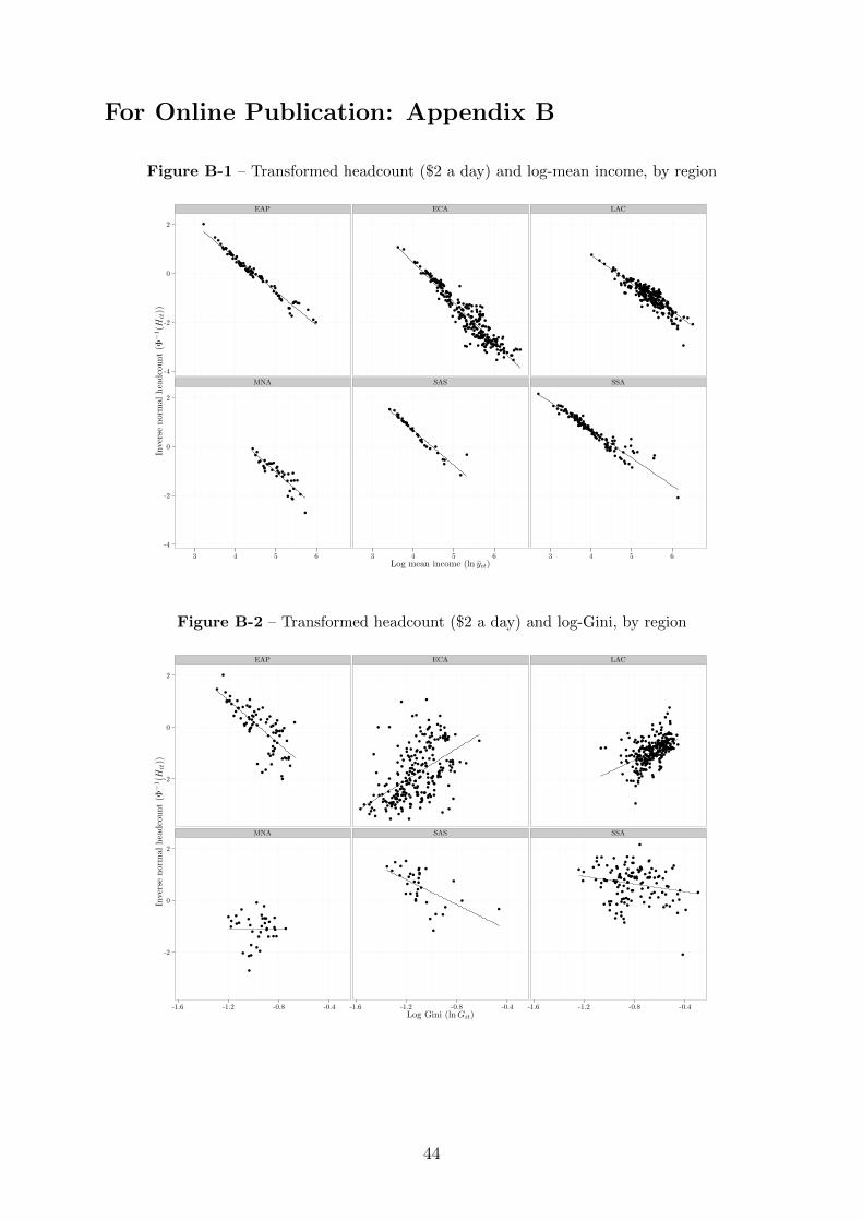
For Online Publication: Appendix B
Figure B-1 – Transformed headcount ($2 a day) and log-mean income, by region
EAP ECA LAC
MNA SAS SSA
-4
-2
0
2
-4
-2
0
2
3 4 5 6 3 4 5 6 3 4 5 6Log mean income (ln yit)
Inve
rse
norm
al
hea
dco
unt
(Φ−1(H
it))
Figure B-2 – Transformed headcount ($2 a day) and log-Gini, by region
EAP ECA LAC
MNA SAS SSA
-2
0
2
-2
0
2
-1.6 -1.2 -0.8 -0.4 -1.6 -1.2 -0.8 -0.4 -1.6 -1.2 -0.8 -0.4Log Gini (lnGit)
Inve
rse
nor
mal
hea
dco
unt
(Φ−1(H
it))
44
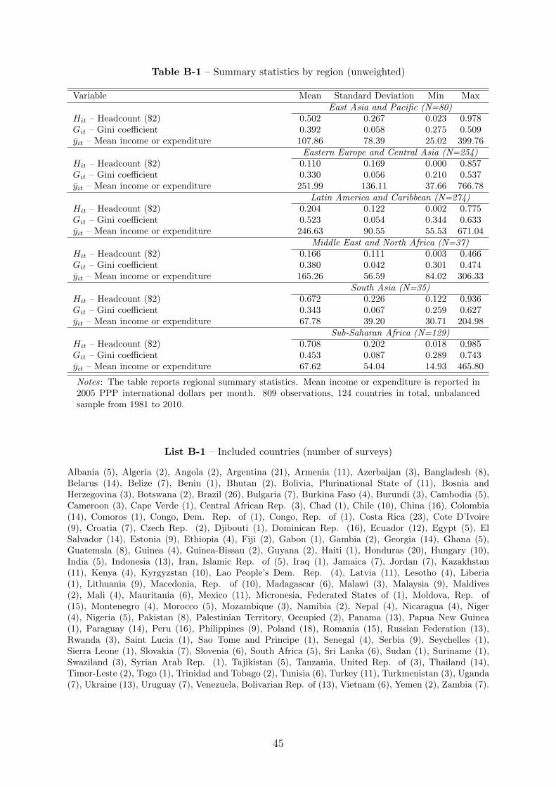
Table B-1 – Summary statistics by region (unweighted)
Variable Mean Standard Deviation Min MaxEast Asia and Pacific (N=80)
Hit – Headcount ($2) 0.502 0.267 0.023 0.978Git – Gini coefficient 0.392 0.058 0.275 0.509yit – Mean income or expenditure 107.86 78.39 25.02 399.76
Eastern Europe and Central Asia (N=254)Hit – Headcount ($2) 0.110 0.169 0.000 0.857Git – Gini coefficient 0.330 0.056 0.210 0.537yit – Mean income or expenditure 251.99 136.11 37.66 766.78
Latin America and Caribbean (N=274)Hit – Headcount ($2) 0.204 0.122 0.002 0.775Git – Gini coefficient 0.523 0.054 0.344 0.633yit – Mean income or expenditure 246.63 90.55 55.53 671.04
Middle East and North Africa (N=37)Hit – Headcount ($2) 0.166 0.111 0.003 0.466Git – Gini coefficient 0.380 0.042 0.301 0.474yit – Mean income or expenditure 165.26 56.59 84.02 306.33
South Asia (N=35)Hit – Headcount ($2) 0.672 0.226 0.122 0.936Git – Gini coefficient 0.343 0.067 0.259 0.627yit – Mean income or expenditure 67.78 39.20 30.71 204.98
Sub-Saharan Africa (N=129)Hit – Headcount ($2) 0.708 0.202 0.018 0.985Git – Gini coefficient 0.453 0.087 0.289 0.743yit – Mean income or expenditure 67.62 54.04 14.93 465.80
Notes: The table reports regional summary statistics. Mean income or expenditure is reported in2005 PPP international dollars per month. 809 observations, 124 countries in total, unbalancedsample from 1981 to 2010.
List B-1 – Included countries (number of surveys)
Albania (5), Algeria (2), Angola (2), Argentina (21), Armenia (11), Azerbaijan (3), Bangladesh (8),Belarus (14), Belize (7), Benin (1), Bhutan (2), Bolivia, Plurinational State of (11), Bosnia andHerzegovina (3), Botswana (2), Brazil (26), Bulgaria (7), Burkina Faso (4), Burundi (3), Cambodia (5),Cameroon (3), Cape Verde (1), Central African Rep. (3), Chad (1), Chile (10), China (16), Colombia(14), Comoros (1), Congo, Dem. Rep. of (1), Congo, Rep. of (1), Costa Rica (23), Cote D’Ivoire(9), Croatia (7), Czech Rep. (2), Djibouti (1), Dominican Rep. (16), Ecuador (12), Egypt (5), ElSalvador (14), Estonia (9), Ethiopia (4), Fiji (2), Gabon (1), Gambia (2), Georgia (14), Ghana (5),Guatemala (8), Guinea (4), Guinea-Bissau (2), Guyana (2), Haiti (1), Honduras (20), Hungary (10),India (5), Indonesia (13), Iran, Islamic Rep. of (5), Iraq (1), Jamaica (7), Jordan (7), Kazakhstan(11), Kenya (4), Kyrgyzstan (10), Lao People’s Dem. Rep. (4), Latvia (11), Lesotho (4), Liberia(1), Lithuania (9), Macedonia, Rep. of (10), Madagascar (6), Malawi (3), Malaysia (9), Maldives(2), Mali (4), Mauritania (6), Mexico (11), Micronesia, Federated States of (1), Moldova, Rep. of(15), Montenegro (4), Morocco (5), Mozambique (3), Namibia (2), Nepal (4), Nicaragua (4), Niger(4), Nigeria (5), Pakistan (8), Palestinian Territory, Occupied (2), Panama (13), Papua New Guinea(1), Paraguay (14), Peru (16), Philippines (9), Poland (18), Romania (15), Russian Federation (13),Rwanda (3), Saint Lucia (1), Sao Tome and Principe (1), Senegal (4), Serbia (9), Seychelles (1),Sierra Leone (1), Slovakia (7), Slovenia (6), South Africa (5), Sri Lanka (6), Sudan (1), Suriname (1),Swaziland (3), Syrian Arab Rep. (1), Tajikistan (5), Tanzania, United Rep. of (3), Thailand (14),Timor-Leste (2), Togo (1), Trinidad and Tobago (2), Tunisia (6), Turkey (11), Turkmenistan (3), Uganda(7), Ukraine (13), Uruguay (7), Venezuela, Bolivarian Rep. of (13), Vietnam (6), Yemen (2), Zambia (7).
45
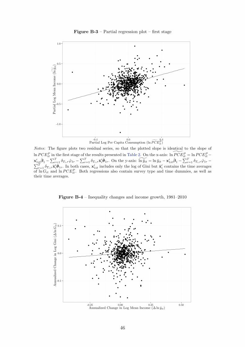
Figure B-3 – Partial regression plot – first stage
-1.0
-0.5
0.0
0.5
1.0
-0.4 0.0 0.4Partial Log Per Capita Consumption ( ˜lnPCEP
it )
Par
tial
Log
Mea
nIn
com
e(˜ lny i
t)
Notes: The figure plots two residual series, so that the plotted slope is identical to the slope of
lnPCEPit in the first stage of the results presented in Table 2. On the x-axis: ˜lnPCEPit = lnPCEPit−x′1itβ1 −
∑Tr=1 δTi,rϕ1r −
∑Tr=1 δTi,rx
′iθ1r. On the y-axis: ln yit = ln yit − x′1itβ1 −
∑Tr=1 δTi,rϕ1r −∑T
r=1 δTi,rx′iθ1r. In both cases, x′1it includes only the log of Gini but x′i contains the time averages
of lnGit and lnPCEPit . Both regressions also contain survey type and time dummies, as well astheir time averages.
Figure B-4 – Inequality changes and income growth, 1981–2010
-0.1
0.0
0.1
-0.25 0.00 0.25 0.50Annualized Change in Log Mean Income (∆ ln yit)
Annualize
dC
hange
inL
og
Gin
i(∆
lnG
it)
46
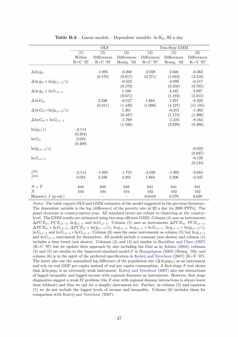
Table B-2 – Linear models – Dependent variable: lnHit, $2 a day
OLS Two-Step GMM(1) (2) (3) (4) (5) (6)
Within Differences Differences Differences Differences DifferencesR+C ’97 R+C ’97 Bourg. ’03 R+C ’97 Bourg. ’03 K+V ’07
∆ ln yit -1.895 -0.268 -2.028 2.046 -0.362(0.170) (0.617) (0.271) (1.043) (3.216)
∆ ln yit × ln(yi,t−1/z) -0.552 -0.995 -0.517(0.179) (0.258) (0.785)
∆ ln yit × lnGi,t−1 1.108 3.445 2.097(0.671) (1.192) (2.315)
∆ lnGit 2.336 -0.527 1.664 1.257 -8.222(0.311) (1.449) (1.008) (4.127) (11.185)
∆ lnGit×ln(yi,t−1/z) 1.261 -0.315 -1.382(0.427) (1.172) (1.996)
∆ lnGit × lnGi,t−1 -1.769 -1.416 -8.164(1.586) (3.929) (8.296)
ln(yit/z) -2.114(0.204)
lnGit 3.024(0.409)
ln(yi,t−1/z) -0.023(0.037)
lnGi,t−1 -0.129(0.134)
¯εHy -2.114 -1.895 -1.755 -2.028 -1.905 -2.684¯εHG 3.024 2.336 2.201 1.664 2.206 -2.345
N × T 648 648 648 641 641 641N 104 104 104 102 102 102Hansen’s J (p-val.) – – – 0.0418 0.579 0.639
Notes: The table reports OLS and GMM estimates of the model suggested in the previous literature.The dependent variable is the log (difference) of the poverty rate at $2 a day (in 2005 PPPs). Thepanel structure is country-survey-year. All standard errors are robust to clustering at the country-level. The GMM results are estimated using two-step efficient GMM. Column (4) uses as instruments∆PCEit, PCEi,t−1, ln yi,t−1 and lnGi,t−1. Column (5) uses as instruments ∆PCEit, PCEi,t−1,∆PCEit × lnGi,t−1, ∆PCEit × ln(yi,t−1/z), ln yi,t−1, ln yi,t−1 × lnGi,t−1, ln yi,t−1 × ln(yi,t−1/z),lnGi,t−1 and lnGi,t−1× lnGi,t−1. Column (6) uses the same instruments as column (5) but ln yi,t−1
and lnGi,t−1 instrument for themselves. All models include a constant (not shown) and column (1)includes a time trend (not shown). Columns (2) and (4) are similar to Ravallion and Chen (1997)(R+C ’97) but we update their approach by also including the Gini as in Adams (2004); columns(3) and (5) are similar to the ‘improved standard model 2’ in Bourguignon (2003) (Bourg. ’03); andcolumn (6) is in the spirit of the preferred specification in Kalwij and Verschoor (2007) (K+V ’07).The latter also use the annualized log difference of the population size (∆ ln popit) as an instrumentand rely on real GDP per capita instead of real per capita consumption. A first-stage F -test showsthat ∆ ln popit is an extremely weak instrument. Kalwij and Verschoor (2007) also use interactionsof lagged inequality and lagged income with regional dummies as instruments. However, first stagediagnostics suggest a weak IV problem (the F -stat with regional dummy interactions is always lowerthan without) and thus we opt for a simpler instrument set. Further, in column (5) and equation(5) we do not include the lagged levels of income and inequality. Column (6) includes them forcomparison with Kalwij and Verschoor (2007).
47
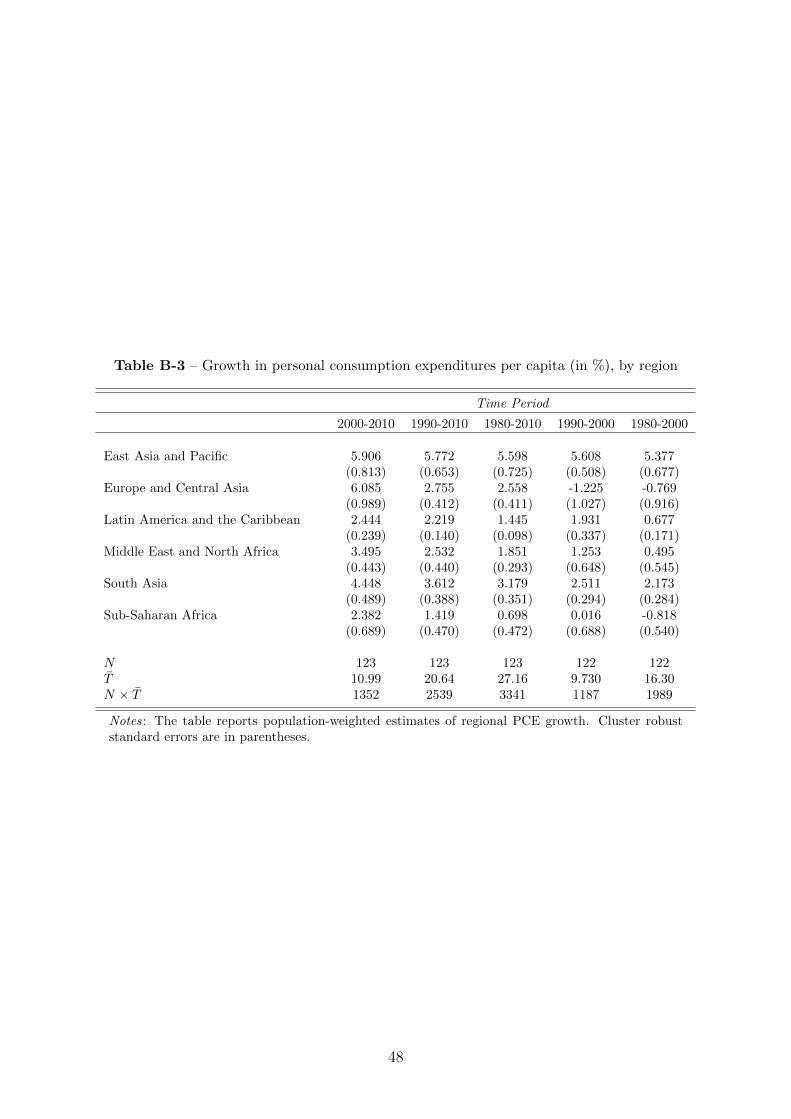
Table B-3 – Growth in personal consumption expenditures per capita (in %), by region
Time Period
2000-2010 1990-2010 1980-2010 1990-2000 1980-2000
East Asia and Pacific 5.906 5.772 5.598 5.608 5.377(0.813) (0.653) (0.725) (0.508) (0.677)
Europe and Central Asia 6.085 2.755 2.558 -1.225 -0.769(0.989) (0.412) (0.411) (1.027) (0.916)
Latin America and the Caribbean 2.444 2.219 1.445 1.931 0.677(0.239) (0.140) (0.098) (0.337) (0.171)
Middle East and North Africa 3.495 2.532 1.851 1.253 0.495(0.443) (0.440) (0.293) (0.648) (0.545)
South Asia 4.448 3.612 3.179 2.511 2.173(0.489) (0.388) (0.351) (0.294) (0.284)
Sub-Saharan Africa 2.382 1.419 0.698 0.016 -0.818(0.689) (0.470) (0.472) (0.688) (0.540)
N 123 123 123 122 122T 10.99 20.64 27.16 9.730 16.30N × T 1352 2539 3341 1187 1989
Notes: The table reports population-weighted estimates of regional PCE growth. Cluster robuststandard errors are in parentheses.
48
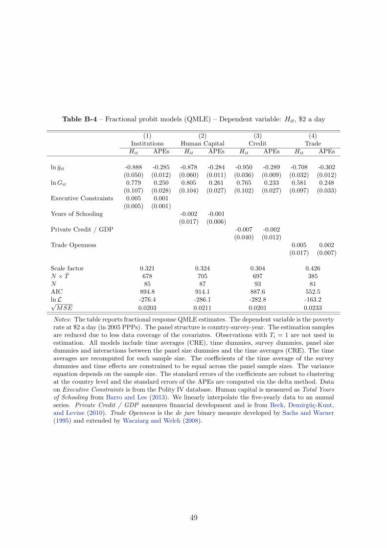
Table B-4 – Fractional probit models (QMLE) – Dependent variable: Hit, $2 a day
(1) (2) (3) (4)Institutions Human Capital Credit TradeHit APEs Hit APEs Hit APEs Hit APEs
ln yit -0.888 -0.285 -0.878 -0.284 -0.950 -0.289 -0.708 -0.302(0.050) (0.012) (0.060) (0.011) (0.036) (0.009) (0.032) (0.012)
lnGit 0.779 0.250 0.805 0.261 0.765 0.233 0.581 0.248(0.107) (0.028) (0.104) (0.027) (0.102) (0.027) (0.097) (0.033)
Executive Constraints 0.005 0.001(0.005) (0.001)
Years of Schooling -0.002 -0.001(0.017) (0.006)
Private Credit / GDP -0.007 -0.002(0.040) (0.012)
Trade Openness 0.005 0.002(0.017) (0.007)
Scale factor 0.321 0.324 0.304 0.426N × T 678 705 697 385N 85 87 93 81AIC 894.8 914.1 887.6 552.5lnL -276.4 -286.1 -282.8 -163.2√MSE 0.0203 0.0211 0.0201 0.0233
Notes: The table reports fractional response QMLE estimates. The dependent variable is the povertyrate at $2 a day (in 2005 PPPs). The panel structure is country-survey-year. The estimation samplesare reduced due to less data coverage of the covariates. Observations with Ti = 1 are not used inestimation. All models include time averages (CRE), time dummies, survey dummies, panel sizedummies and interactions between the panel size dummies and the time averages (CRE). The timeaverages are recomputed for each sample size. The coefficients of the time average of the surveydummies and time effects are constrained to be equal across the panel sample sizes. The varianceequation depends on the sample size. The standard errors of the coefficients are robust to clusteringat the country level and the standard errors of the APEs are computed via the delta method. Dataon Executive Constraints is from the Polity IV database. Human capital is measured as Total Yearsof Schooling from Barro and Lee (2013). We linearly interpolate the five-yearly data to an annualseries. Private Credit / GDP measures financial development and is from Beck, Demirguc-Kunt,and Levine (2010). Trade Openness is the de jure binary measure developed by Sachs and Warner(1995) and extended by Wacziarg and Welch (2008).
49
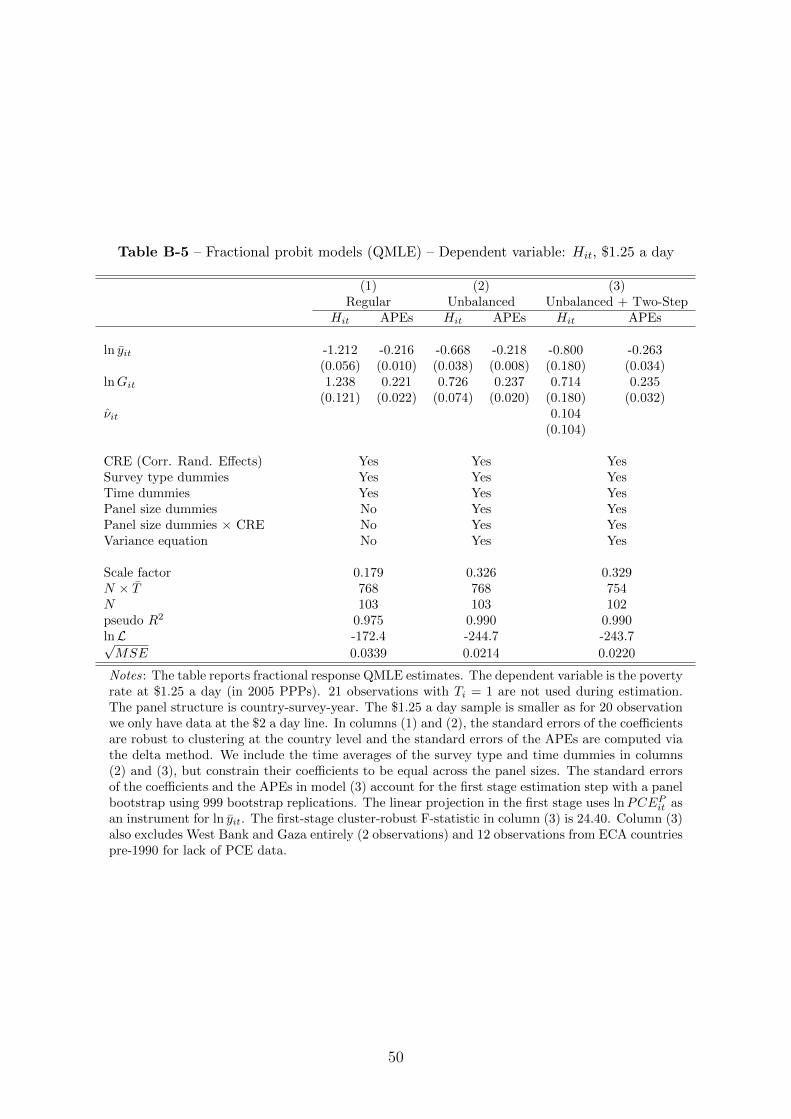
Table B-5 – Fractional probit models (QMLE) – Dependent variable: Hit, $1.25 a day
(1) (2) (3)Regular Unbalanced Unbalanced + Two-Step
Hit APEs Hit APEs Hit APEs
ln yit -1.212 -0.216 -0.668 -0.218 -0.800 -0.263(0.056) (0.010) (0.038) (0.008) (0.180) (0.034)
lnGit 1.238 0.221 0.726 0.237 0.714 0.235(0.121) (0.022) (0.074) (0.020) (0.180) (0.032)
νit 0.104(0.104)
CRE (Corr. Rand. Effects) Yes Yes YesSurvey type dummies Yes Yes YesTime dummies Yes Yes YesPanel size dummies No Yes YesPanel size dummies × CRE No Yes YesVariance equation No Yes Yes
Scale factor 0.179 0.326 0.329N × T 768 768 754N 103 103 102pseudo R2 0.975 0.990 0.990lnL -172.4 -244.7 -243.7√MSE 0.0339 0.0214 0.0220
Notes: The table reports fractional response QMLE estimates. The dependent variable is the povertyrate at $1.25 a day (in 2005 PPPs). 21 observations with Ti = 1 are not used during estimation.The panel structure is country-survey-year. The $1.25 a day sample is smaller as for 20 observationwe only have data at the $2 a day line. In columns (1) and (2), the standard errors of the coefficientsare robust to clustering at the country level and the standard errors of the APEs are computed viathe delta method. We include the time averages of the survey type and time dummies in columns(2) and (3), but constrain their coefficients to be equal across the panel sizes. The standard errorsof the coefficients and the APEs in model (3) account for the first stage estimation step with a panelbootstrap using 999 bootstrap replications. The linear projection in the first stage uses lnPCEPit asan instrument for ln yit. The first-stage cluster-robust F-statistic in column (3) is 24.40. Column (3)also excludes West Bank and Gaza entirely (2 observations) and 12 observations from ECA countriespre-1990 for lack of PCE data.
50
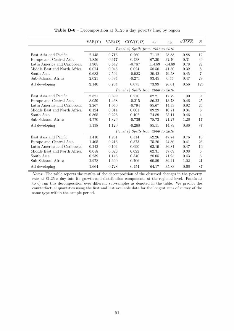
Table B-6 – Decomposition at $1.25 a day poverty line, by region
VAR(Y ) VAR(D) COV(Y,D) sY sD√MSE N
Panel a) Spells from 1981 to 2010
East Asia and Pacific 2.145 0.716 0.260 71.12 28.88 0.88 12Europe and Central Asia 1.856 0.677 0.438 67.30 32.70 0.31 39Latin America and Caribbean 1.905 0.642 -0.787 114.89 -14.89 0.78 28Middle East and North Africa 0.074 0.045 0.024 58.50 41.50 0.32 8South Asia 0.683 2.594 -0.023 20.42 79.58 0.45 7Sub-Saharan Africa 2.021 0.394 -0.271 93.45 6.55 0.47 29
All developing 2.140 0.704 0.075 73.99 26.01 0.56 123
Panel c) Spells from 2000 to 2010
East Asia and Pacific 2.821 0.399 0.270 82.21 17.79 1.00 9Europe and Central Asia 8.059 1.468 -0.215 86.22 13.78 0.46 25Latin America and Caribbean 2.267 1.040 -0.794 85.67 14.33 0.92 26Middle East and North Africa 0.124 0.014 0.001 89.29 10.71 0.34 6South Asia 0.865 0.223 0.102 74.89 25.11 0.46 4Sub-Saharan Africa 4.770 1.826 -0.736 78.73 21.27 1.26 17
All developing 5.138 1.120 -0.268 85.11 14.89 0.86 87
Panel c) Spells from 2000 to 2010
East Asia and Pacific 1.410 1.261 0.314 52.26 47.74 0.76 10Europe and Central Asia 1.405 0.213 0.373 75.20 24.80 0.41 26Latin America and Caribbean 0.243 0.104 0.090 63.19 36.81 0.47 19Middle East and North Africa 0.058 0.026 0.022 62.31 37.69 0.38 5South Asia 0.239 1.146 0.340 28.05 71.95 0.43 6Sub-Saharan Africa 2.978 1.690 0.706 60.59 39.41 1.02 21
All developing 1.664 0.728 0.454 64.17 35.83 0.66 87
Notes: The table reports the results of the decomposition of the observed changes in the povertyrate at $1.25 a day into its growth and distribution components at the regional level. Panels a)to c) run this decomposition over different sub-samples as denoted in the table. We predict thecounterfactual quantities using the first and last available data for the longest runs of survey of thesame type within the sample period.
51
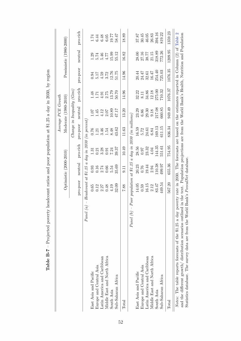
Table
B-7
–P
roje
cted
pov
erty
hea
dco
unt
rati
osan
dp
oor
pop
ula
tion
at$1
.25
ad
ayin
2030
,by
regi
on
Ave
rage
PC
EG
row
th
Op
tim
isti
c(2
000-2
010)
Mod
erate
(1980-2
010)
Pes
sim
isti
c(1
980-2
000)
Chan
gein
Ineq
uali
ty(G
ini)
pro
-poor
neu
tral
pro
-ric
hp
ro-p
oor
neu
tral
pro
-ric
hp
ro-p
oor
neu
tral
pro
-ric
h
Pan
el(a
)–
Hea
dco
un
tat$1
.25
aday
in2030
(in
perc
ent)
Eas
tA
sia
and
Pac
ific
0.6
50.9
31.3
10.7
61.0
71.4
80.9
41.2
91.7
4E
uro
pe
and
Cen
tral
Asi
a0.1
20.1
60.2
11.2
11.4
51.7
15.1
75.7
46.4
4L
atin
Am
eric
aan
dC
arib
bea
n2.2
72.7
43.2
83.4
64.1
24.9
14.5
95.4
66.4
8M
idd
leE
ast
and
Nor
thA
fric
a0.4
80.6
60.9
11.5
42.0
72.7
53.7
24.7
76.0
5S
outh
Asi
a4.1
95.5
47.2
48.4
810.8
913.7
912.7
615.9
919.7
7S
ub
-Sah
aran
Afr
ica
32.0
935.6
939.3
743.6
247.1
750.7
051.7
555.1
258.4
7
Tot
al7.8
89.1
110.4
911.6
313.2
014.9
614.9
616.8
218.8
9
Pan
el(b
)–
Poo
rpo
pu
lati
on
at$1.2
5a
day
in2030
(in
mil
lion
s)
Eas
tA
sia
and
Pac
ific
14.0
520.2
328.5
616.5
923.2
932.2
220.4
428.0
037.8
7E
uro
pe
and
Cen
tral
Asi
a0.5
90.7
60.9
75.7
26.8
68.1
124.4
727.1
630.4
5L
atin
Am
eric
aan
dC
arib
bea
n16.1
519.4
423.3
224.6
129.3
034.8
632.6
138.7
746.0
5M
idd
leE
ast
and
Nor
thA
fric
a2.1
22.9
44.0
46.8
49.1
812.1
816.4
721.1
526.8
3S
outh
Asi
a83.4
7110.3
8144.3
5169.1
3217.0
8275.0
0254.4
0318.8
9394.1
6S
ub
-Sah
aran
Afr
ica
449.5
4499.9
7551.6
1611.1
5660.8
5710.3
2725.0
3772.2
6819.2
2
Tot
al567.2
0655.3
6754.9
5836.3
4949.4
91076.3
71076.3
51209.9
51359.2
3
Note
s:T
he
tab
lere
por
tsfo
reca
sts
ofth
e$1
.25
ad
ayp
over
tyra
tein
2030.
Th
efo
reca
sts
are
base
don
the
esti
mate
sre
port
edin
Colu
mn
(2)
of
Tab
le2
and
the
diff
eren
tgr
owth
/d
istr
ibuti
onsc
enar
ios
outl
ined
inth
ete
xt.
Popu
lati
on
pro
ject
ion
sare
from
the
Worl
dB
an
k’s
Hea
lth
,N
utr
itio
nan
dP
op
ula
tion
Sta
tist
ics
dat
abas
e.T
he
surv
eyd
ata
are
from
the
Wor
ldB
an
k’s
Povc
alN
etd
ata
base
.
52