Embed Size (px)
Citation preview

i
Potential Water Supply of the Mnyabezi Catchment
A case study of a small reservoir and alluvial aquifer system
in the arid region of southern Zimbabwe
Enschede, July 2007
Wouter de Hamer

ii
Title
Potential Water Supply of the Mnyabezi Catchment: a case study of a small
reservoir and alluvial aquifer system in the arid region of southern Zimbabwe
Author Wouter de Hamer
Date 6 July, 2007
Project
This study represents Wouter de Hamer’s thesis to the MSc degree in
Water Engineering & Management at the University of Twente.
Graduation Committee prof. dr. ir. A.Y. Hoekstra University of Twente
dr. ir. M.J. Booij University of Twente
D. Love MSc WaterNet, Zimbabwe
Contact: [email protected] [email protected]

iii
Acknowledgements
Six months ago, I started to work on this research for my graduation to the MSc degree in Water
Engineering & Management at the University of Twente. At the end of this period, the time has come
to evaluate my research and thank some people who were very important for me.
Zimbabwe is not the first country thinking of for your graduation, because of its bad political and
economical situation, but I have experienced these working conditions as a challenge. On the 6th of
February, I flew to Harare knowing nothing more than the name of my supervisor, the company I
would work for and the address I would sleep at. Already in the first week, I visited my study area in
southern Zimbabwe, met several local people, experienced the African hospitality and knew this
would become a fabulous time. Due to the alternation between fieldwork and desktop work, and the
integration between several subjects in the field of geology, hydrology, ecology, soil science and water
resource management, I have experienced my graduation period as very interesting and pleasant time.
Several people have assisted me during my research. First, I would like to thank my supervisors.
Martijn, you always responded very elaborately on my questions, which was of great importance to
improve my report adequately. Arjen, thank for the opportunity you gave me to do my graduation in
Zimbabwe and your comments on mainly the structure of the report. David, your invitation to stay at
your home in Zimbabwe says much about your hospitality and kindness. Thanks for your assistance
and great time in Zimbabwe! I wish you all the best coming years with Faith and your daughter
Kathleen. Patrick and Tutanang, I owe you much gratitude for your help during my field trips and the
daily readings of the measuring equipments. Richard, your experience with the MODFLOW-model
was of great help to me. At last, I would like to thank the people at WaterNet - Zimbabwe, ICRISAT -
Bulawayo, Dabane Trust, the Zimbabwean Water Authority (ZINWA), the department of Civil
Engineering and the department of Geology at the University of Zimbabwe for facilitating me with
several things during my research period.
At last, I would like to thank my parents for supporting me during my whole study period. Thanks, for
giving me the opportunities to explore the life as a student in Enschede and abroad.
Enschede, July 2007
Wouter de Hamer

iv
Abstract
In the arid regions of southern Zimbabwe, dam reservoirs normally meet the domestic and agricultural
water requirements of smallholder farmers in dry periods. Groundwater use by accessing alluvial
aquifers of non-perennial rivers can be an important extra water resource. However, the storage
capacity of alluvial aquifers is not used very intensively in southern Zimbabwe at this moment. The
research objective is to calculate the potential water supply for the upper-Mnyabezi catchment in the
arid region of southern Zimbabwe under current conditions and after implementation of two storage
capacity measures. These measures are heightening the spillway of the Mnyabezi dam and
constructing a sand storage dam in the alluvial aquifer of the Mnyabezi River. The upper-Mnyabezi
catchment covers 22 km2 and is a tributary of the Thuli River in southern Zimbabwe.
In this study, three coupled models are used to simulate the hydrological processes in the Mnyabezi
catchment. The first is a rainfall-runoff model, based on the SCS-method. The second model is a
spreadsheet-based water balance model of the dam reservoir, which is used to calculate the water level
in the reservoir. This model has three functions; i) simulate the water balance of the reservoir, ii)
calculate the potential water supply and iii) calculate the days of dam overflow. The finite difference
groundwater model MODFLOW is used to simulate the water balance and drying process of the
alluvial aquifer for a section of 1.0 km downstream of the Mnyabezi dam. For the calibration process,
daily measured data from the period March to May 2007 is used.
Under current conditions, the period of water supply ranges from 5.7 months in an extreme dry year
(total amount of water supply is 2,107 m3) to 8.7 months in an extreme wet year (total amount of water
supply is 3,162 m3). In the case of a heightened spillway, the potential water supply increases
respectively with 417 m3 and 139 m3. When constructing a sand storage dam in the alluvial aquifer,
the potential water supply increases respectively with 252 m3 and 316 m3. After these two water
management measures are implemented, the maximum period of water supply in an extreme dry year
is 8.4 months (total amount of water supply is 2,776 m3) and in an extreme wet year 10.8 months (total
amount of water supply is 3,617 m3).
For the Mnyabezi catchment, the alluvial aquifer is too small to sustain a storage capacity large
enough to supply water whole year round. Thus, a sand storage dam can only be used as an additional
water resource. However, when an ephemeral river is underlain by a larger alluvial aquifer, a sand
storage dam is a promising way of water supply for smallholder farmers in southern Zimbabwe.

1
Contents
1. Introduction ......................................................................................................................................... 3 1.1 UN Millennium Development Goals............................................................................................. 3 1.2 Water availability in southern Africa ............................................................................................ 3 1.3 WaterNet Challenge Program on Food and Water........................................................................ 5 1.4 Project scope ................................................................................................................................. 5 1.5 Research objective......................................................................................................................... 6 1.6 Outline........................................................................................................................................... 7
2. Literature Study................................................................................................................................... 8 2.1 Definition of the river continuum.................................................................................................. 8 2.2 Hydrological characteristics of alluvial aquifers ........................................................................... 9 2.3 Water balance of an alluvial aquifer system................................................................................ 11 2.4 Water use in arid regions............................................................................................................. 12
3. Study Area......................................................................................................................................... 14 3.1 General characteristics of the Mnyabezi catchment .................................................................... 14 3.2 Precipitation in the Mnyabezi catchment .................................................................................... 15 3.3 Evapotranspiration in the Mnyabezi catchment .......................................................................... 15 3.4 Hydrogeological characteristics of the Mnyabezi catchment...................................................... 16
4. Method .............................................................................................................................................. 17 4.1 Calculation potential water supply .............................................................................................. 17 4.2 Rainfall-runoff model.................................................................................................................. 18 4.3 Reservoir model .......................................................................................................................... 19 4.4 Groundwater model ..................................................................................................................... 19 4.5 Measuring strategy ...................................................................................................................... 21 4.6 Calibration method ...................................................................................................................... 25

2
5. Results field measurements ............................................................................................................... 28 5.1 Rainfall-runoff model.................................................................................................................. 28 5.2 Reservoir model .......................................................................................................................... 30 5.3 Groundwater model ..................................................................................................................... 31
6. Results models................................................................................................................................... 36 6.1 Sensitivity of the reservoir and rainfall-runoff models ............................................................... 36 6.2 Calibration of the reservoir and rainfall-runoff models............................................................... 37 6.3 Sensitivity of the groundwater model.......................................................................................... 38 6.4 Calibration of the groundwater model......................................................................................... 39 6.5 Uncertainty in outcomes.............................................................................................................. 39
7. Analysis............................................................................................................................................. 42 7.1 Water balance of the Mnyabezi reservoir.................................................................................... 42 7.2 Potential water supply of the Mnyabezi reservoir ....................................................................... 43 7.3 Water balance of the alluvial aquifer........................................................................................... 44 7.4 Potential water supply alluvial aquifer ........................................................................................ 45 7.5 Discussion ................................................................................................................................... 46
8. Conclusions ....................................................................................................................................... 48
References ............................................................................................................................................. 50
Appendices ............................................................................................................................................ 54

3
1. Introduction
This chapter introduces the water resource management problems in (semi-)arid regions and in
particular to the Limpopo basin. Furthermore, this chapter provides insight into the way this MSc-
thesis contributes to these problems by defining a research scope and objective. At last, an outline for
the report is presented.
1.1 UN Millennium Development Goals
In the year 2000, the governments of the world adopted eight UN Millennium Development Goals as a
blueprint to achieve a better world in the 21st century. These Millennium Development Goals try to
meet the needs of the world’s poorest on issues like poverty, health and education. The first
millennium goal is to halve the proportion of people who suffer from hunger between 1990 and 2015
(UN Millennium Project, 2005). Approximately 50 % of the 850 million people living in serious and
chronic hunger worldwide are smallholder farmers (FAO, 2004). For this reason the Millennium
Project recommendations on rural development and food security focuses on improving the production
and livelihoods of smallholder farmers (UN Millennium Project, 2005).
The Millennium Development Goals’ target to halve the proportion of people who suffer from hunger
is extremely important in southern Africa, where food security has become increasingly problematic.
Although the poverty rate declined marginally, the number of people living in extreme poverty in
southern Africa increased by 140 million between 1990 and 2005 (UN Millennium Project, 2005).
Agriculture by smallholder farmers is the dominant economic activity in these countries, accounting
for approximately 70 % of total employment (Love et al., 2006). Despite the technological advances in
agricultural research in recent years, poverty, food insecurity and malnutrition remain major
challenges in southern Africa (Sanchez & Swami Nathan, 2005).
1.2 Water availability in southern Africa
Agriculture by smallholder farmers in southern Africa is largely rain fed, which is risky in the event of
recurrent droughts (Twomlow & Bruneau, 2000). A drought is a period of months or years in which a
region suffers from a deficit in its water supply. A deficit in water supply occurs when the amount of
available water is not enough to meet the local agricultural and domestic water requirements. To
unlock paths for more food security and to improve the livelihoods of smallholder farmers, integrated

4
water resource management (IWRM) is a basic requirement (Falkenmark & Rockström, 2003). IWRM
is defined by Mostert et al. (1999) as “the management of the water system, being part of the broader
natural environment and in relation to their socio-economic environment”.
An example of a poverty-stricken area in southern Africa is the Limpopo basin (see figure 1Figure 1).
The basin covers an area of approximately 282,000 km2 and is draining an extensive area of Botswana,
South Africa, Zimbabwe and Mozambique. Approximately 14 million people live in this basin area.
Translating IWRM from concept to action, to secure water availability and food production for
smallholder farmers, remains largely undone in this area (Love et al., 2004). New policies and
structures developed by the water reforms since 1990 do not generally penetrate to the smallholder
farmer (Jaspers, 2003). Water policy and institutions in the Limpopo Basin are mainly concerned with
water for large-scale irrigation, cities, mines and industry, while rain fed agriculture is sustaining the
production of smallholder farmers (Love et al., 2004).
Figure 1: The Limpopo basin; the red dot indicates the location of the Mnyabezi catchment (INGC, 2003)
The rain fed production of food in semi-arid regions is risky and crop failure often occurs (Mwenge
Kahinda, 2004; Mwakalila, 2006). Besides, many smallholder farmers cultivate on poor soils, which
makes crop yields low (Twomlow & Bruneau, 2000). Mwakalila (2006) demonstrated for an arid area
in Tanzania that the return on labour for smallholder farmers who irrigate their fields is about three
times as high as smallholder farmers who cultivate rain-fed fields. Nevertheless, access to irrigation

5
water for smallholder farmers remains limited in the Limpopo basin (Love et al., 2006). In the past,
large-scale irrigation projects for food security have often failed due to the high maintenance costs.
Therefore, the Millennium Project urges the use of appropriate irrigation technology such as low-cost
drip kits (Moyo et al., 2006). Drip technology tends to improve water use efficiency, compared to the
initial situation, but does not always increase yield especially during dry seasons (Maisiri et al., 2005).
Alternatively, the availability of water can be improved through agricultural interventions in dry land
farming (Twomlow et al., 1999; Woltering, 2005), through supplementary irrigation using rainwater
harvesting (Mwenge Kahinda, 2004) or by accessing alluvial aquifers (Dahlin & Owen, 2005; Moyce
et al., 2006).
1.3 WaterNet Challenge Program on Food and Water
WaterNet is a regional network in southern Africa of university departments and research and training
institutes specialized in water resource management. The mission of WaterNet is to “enable the people
of southern Africa to efficiently and effectively manage their water resources” (WaterNet, 2001). As
elaborated on in the previous section, the high-risk failure of rain fed agriculture has a negative
influence on food security in the Limpopo basin. This problem formed the basis for WaterNet to
develop a project under the Challenge Program on Water and Food. The Challenge Program is a
research initiative of the Consultative Group on International Agricultural Research (CGIAR). The
overall goal of the WaterNet Challenge Program is contributing to the improvement of rural
livelihoods of smallholder farmers through the development of an IWRM framework for increased
productive use of water and risk management for drought and dry-spell mitigation at all scales in the
Limpopo basin (WaterNet, 2004). The research focuses on three pilot sub-catchments of the Limpopo
River basin in Zimbabwe (Mzingwane catchment), Mozambique (Chòkwé catchment) and South
Africa (Olifants catchment).
1.4 Project scope
In the arid regions of the world, rivers are mostly non-perennial (do not flow throughout the year).
These arid areas centre along the tropics, north and south of the equator, where over a billion people in
110 countries live on more than 30 % of the Earth’s surface. Twenty African countries have more than
90 % of their productive lands in vulnerable arid regions, illustrating the human dimensions of the
issue (Turnbull, 2002). Although drought is a normal occurrence in arid regions, people are often
unprepared when it happens. Periods of drought often result in increased pressure on the surface and
subsurface water resources as well as the vegetation associated with non-perennial rivers (Seely et al.,
2003).

6
In the arid regions of Zimbabwe, dam reservoirs meet the domestic and agricultural water
requirements of smallholder farmers in dry periods. However, a few months after the main rainy
season these reservoirs dry out during years with little rainfall. Groundwater use by accessing alluvial
aquifers of non-perennial rivers can be an important additional water resource, because in several arid
regions people harvest water from these systems during droughts. Barker & Molle (2004) describe an
alluvial aquifer as a groundwater unit, generally unconfined, hosted in laterally discontinuous layers of
sand, silt and clay and deposited by a river in a river channel, banks or flood plain. On a small scale,
alluvial aquifers in large perennial rivers meet agricultural and domestic water requirements in
southern Africa (Seely et al, 2003; Love, 2006b). The groundwater storage of the alluvial aquifers of
these large rivers, has a large potential water supply (Owen & Dahlin, 2005; Moyce et al., 2006).
However, most smallholder farmers in southern Zimbabwe live near to smaller non-perennial rivers
that make research to groundwater resources in these smaller alluvial aquifers interesting. In this
study, with ‘small non-perennial rivers’ is meant a water systems with a catchment below 500 km2.
This MSc-thesis concentrates on the hydrological processes occurring in the upper-Mnyabezi
catchment. The upper-Mnyabezi catchment covers 22 km2 and is situated in southern Zimbabwe (see
figure 1; the red dot indicates the location of the catchment). Water is stored in the Mnyabezi dam
reservoir (caused by human intervention) and in the alluvial aquifer of the Mnyabezi River (which is a
natural process). These two ways of water storage ensure a water resource during the dry season for
plants, animals and people, but is still not enough to bridge the gap of surface water shortage in a
normal or dry year. Possible water management interventions to improve the total storage in the upper-
Mnyabezi catchment are the heightening of the spillway of the reservoir dam, and the construction of a
sand storage dam in the alluvial aquifer.
1.5 Research objective
The research objective is to calculate the potential water supply for the upper-Mnyabezi catchment in
the arid region of southern Zimbabwe for current conditions and after implementation of two storage
capacity measures. These measures are heightening the spillway of the Mnyabezi dam reservoir and
constructing a sand storage dam in the alluvial aquifer of the Mnyabezi River.
What is not included
The study concentrates on surface water and sub-surface groundwater. Thus, it does not monitor
groundwater storage in deeper layers. Furthermore, the research does not focus on the water quality.
Possible long-term changes in input parameters and variables, for example due to climate change or
change in land use, has not been taken into account as well.

7
Research questions
The formulation of research questions is important to acquire the knowledge, which is essential to
answer the research objective.
a) What are the hydro(geo)logical characteristics of the upper-Mnyabezi catchment, the
Mnyabezi dam reservoir and the alluvial aquifer system of the Mnyabezi River?
b) What are the relations between the inflows and outflows (water balance) of the upper-
Mnyabezi catchment, the Mnyabezi dam reservoir and the alluvial aquifer system of the
Mnyabezi River?
c) What are the influences on the amount of water supply, when heightening the spillway of the
Mnyabezi dam reservoir and constructing a sand storage dam in the alluvial aquifer of the
Mnyabezi River?
1.6 Outline
This report provides insight into the hydrological processes in a small catchment in the arid regions of
southern Zimbabwe. The results contribute to the drought problems in small catchments in the
Limpopo Basin as explained in section 1.2. The second chapter describes the theoretical background
information about alluvial aquifer systems. The third chapter explains the characteristics of the study
area. The fourth chapter clarifies the research, modelling and measuring methods. The fifth chapter
presents the field measurement results and the sixth chapter the results of the calibration of the models.
The seventh chapter is dedicated to the analysis of the results and the calculation of the potential water
supply. The study ends with the conclusion of the MSc-thesis.

8
2. Literature Study
This chapter explains the theoretical concepts used in this MSc-thesis, concentrating on alluvial
aquifer systems. The first section explains the definition of the river continuum. The second and third
sections describe the complex water system of alluvial aquifer. The last section provides a review
about the water use of alluvial aquifer systems and reservoirs of non-perennial rivers in arid regions of
southern Africa.
2.1 Definition of the river continuum
In humid climates, rivers are generally perennial. Perennial rivers are characterized by periodic high
flow events of varying magnitude and duration (occurring in response to individual rainfall events),
superimposed on continuous, more slowly varying low flows derived from drainage out of catchment
storages, including soil moisture, ground water and surface water (Hughes, 2005). In arid regions,
most rivers are non-perennial (also referred to as temporal). Regarding hydroclimatic conditions,
several different definitions of a (semi-)arid tropical environment exist. In this study the definition
mentioned by Sandstrom (1997), based on annual values of rainfall in tropical dry lands, is used;
500 – 900 mm is semi-arid, 200 – 500 mm is arid and less than 200 mm per year is a hyper-arid area.
Perennial seasonal
Perennial aseasonal
Intermittent aseasonal
Intermittent seasonal
Ephemeral: flow for short periods during the year
Flow variability increasesNatural distribution increases
Flow
pre
dict
abili
ty in
crea
ses
Con
nect
ivity
sur
face
hab
itat i
ncre
ases
Biot
ic/a
biot
ic c
ontro
ls in
crea
ses
Surface water flow stops annually or two out of five years
Surface water dissapears
Episodic: flow once in several years
Figure 2: River continuum (Uys & O’Keeffe, 1997)
9
Non-perennial rivers are characterized by the phenomenon that flow stops and surface water may
disappear along parts of the channel either yearly or during two or more years in a five-year period
(Rossouw et al., 2005). Various authors have attempted to classify non-perennial rivers according to
the percentage of annual flow, source of flow and periodicity of flow into for example ephemeral and
intermittent streams. However, other descriptive terms such as seasonal and episodic rivers confuse
the terminology. Uys & O’Keeffe (1997) provide a functional classification for non-perennial rivers
(see figure 2). The most important characteristic of this classification is the definition of two
hydrological state changes, which results in major biotic and a-biotic changes in the river system. The
non-perennial river continuum represents these stages as steps.
The first step is where surface water flow stops, but surface water is still present in pools in the
majority of a channel. The so-called intermittent rivers cease to flow and dry partly for a variable
period during the year, or for two or more years in a five-year period. Flow may recommence
seasonally, or highly variable (a-seasonal), depending on climatic influences and predictability of
rainfall. An intermittent river may experience several cycles of flow and drying in a single year.
The second step is where surface water totally disappears from the majority of the channel. Ephemeral
rivers flow for a shorter period than they are dry. They flow, in response to unpredictable high rainfall
events, for short periods of most years during a five-year period. The rivers support a series of pools in
parts of the channel. Episodic rivers are highly flashy systems that flow or flood only in response to
extreme rainfall events, usually high in their catchments. They may not flow in a five-year period, or
may flow only once in several years.
2.2 Hydrological characteristics of alluvial aquifers
Ephemeral and intermittent rivers primary drain (semi-)arid regions of the world. These arid regions
are typically subjected to occasional high rainfall events and a consequent high degree of surface
erosion (Nord, 1985). The rivers are not able to cope with the large sediment load, which cause
settlement of large amounts of sand within the river channel. As a result, many of the rivers have
become so-called ‘sand rivers’ (Hussey, 2003). ‘Sand rivers’ refer to the dry riverbed and the
underlying alluvial aquifer, which usually contains groundwater throughout the year. Because of their
shallow depth and vicinity to the streambed, alluvial aquifers have a direct relationship with the stream
flow (Townley, 1998) and can significantly contribute to the water balance (De Vries & Simmers,
2002). River flow usually dominates recharge of alluvial aquifers (Nord, 1985; Owen & Dahlin,
2005). As a flood travels down a non-perennial river, water infiltrates into the sandy and gravel
alluvial deposits of the channel beds. The amount of recharge depends on the intensity, volume and
duration of a flood (Heyns et al., 1997). In non-perennial rivers in Botswana and Zimbabwe flow only

10
occurs after the aquifer channel sands have become fully saturated (Nord, 1985; Hughes, 2005; Owen
& Dahlin, 2005). Figure 3 shows the groundwater table development typical for alluvial aquifer
systems. After a rainfall event, the groundwater table declines away from the stream, and thus
groundwater flow leaks away from alluvial aquifer into the underlying granite (Sandstrom, 1997).
Groundwater stored in the riverbed can also be perched above the weathered basement (Wikner, 1980;
Davis et al., 1995; Anderson, 1997). Silt and fine sediments form an almost impermeable seal at the
base of the river channel, which prevent seepage into the underlying basement layer.
Water table
River flow
Saturated sediment
Alluvial aquifer directly after a heavy rain event
Water table
Saturated sediment
Alluvial aquifer some days after a heavy rain event
Water table
Dry sediment
Alluvial aquifer some weeks after a heavy rain event
Water table
Dry sediment
Alluvial aquifer after a long dry period Figure 3: Groundwater development for alluvial aquifer systems (Hussey, 2003)
The recharge of alluvial aquifers ensures a water source during the dry season for plants, animals and
people (Jacobson et al., 1995). The recharge process is therefore fundamental to an understanding of
livelihood conditions and the sustainability of different types of water consuming activities. In arid
areas, evaporation and transpiration have great effect on the hydrological cycle and thereby on the
availability of water for vegetation (Sandstrom, 1997). Wipplinger (1958) and Nord (1985) showed
the evaporation following saturation causing a 0.9 m drop of the groundwater table within three
months. Evaporation stops when the water table recedes 0.9 m below the surface of the sand. Below
this elevation, water is only lost due to evapotranspiration by riparian vegetation and leakage to deeper
layers. Riparian vegetation can determine the character of the river. Gorgens & Lee (1992) show that
removal of vegetation increases the total runoff in a South African catchment. Additionally, when
eucalyptus plantations grow in the riverbanks a perennial river may turn ephemeral.
Despite the high hydraulic conductivity, the groundwater flow through the alluvial aquifers itself is
rather slow due to the gentle slopes. Nord (1985) estimated the water velocity roughly to be about 1 –
2 m per day. During the dry season, the seepage and evapotranspiration are the main losses in alluvial
aquifers. The groundwater flow in these smaller systems even seem to cease towards the end of the dry
season, while there is still a substantial subsurface flow in the larger alluvial aquifers (Nord, 1985).

11
2.3 Water balance of an alluvial aquifer system
Sustainable water resource management requires an understanding of the hydrological processes
dominant in an aquifers-river system (Uhlenbrook et al., 2004), therefore there is a need to quantify
the water balance of such a system. The water balance is the equilibrium between the volume of water
inputs, outputs and net changes over a fixed period in the alluvial aquifer (Shaw, 1994). The water
balances of an alluvial aquifer and a river are presented in equations 1 and 2 (Schicht & Walton, 1961;
Healy & Cook, 2002). Figure 4 visualizes the flows of the water balance of the alluvial aquifer system.
PEQQQQQS pumpseepageleakageoutgroundingroundground +−−+−+−=Δ ,, (1)
outstreaminstreamleakagestream QQQS ,, −+−=Δ (2)
Where all variables are in equal units [mm.day-1],
ΔSground is the change in groundwater storage,
ΔSstream is the change in surface water storage,
Qleakage is the leakage from the river to the aquifer,
Qseepage is the seepage from the alluvial aquifer to the underlying ground layer,
Qpump includes the amount of pumping,
Qground,in – Qground,out is the net groundwater water flows,
Qstream,in – Qstream,out is the net surface water flow,
E is evapotranspiration from the unsaturated zone and
P is the precipitation, which percolates through the unsaturated zone.
RiverE
Water table
Surface
P
Unsaturated groundwater layer
Saturated groundwater layerQground,in Qground,out
Qstream,in Qstream,out
Qpump
Qseepage
Qleakage
Figure 4: Water balance of an alluvial aquifer

12
Figure 4 visualizes the river as an isolated unit, while in nature the stream partially penetrates the
unconfined aquifer (Osman & Bruen, 2002). This distinction between the surface water and
groundwater flows is common in surface-groundwater models (Harbaugh, 2005; Arnold & Fohrer,
2005). The figure does not show lateral flows, but these form a part of the groundwater in- and
outflow as well. In this MSc-thesis, a surface-groundwater model simulates the water balance of a
small section of the Mnyabezi alluvial aquifer system.
Traditionally, groundwater models solve surface water without much detail. Similarly, groundwater
models applied to aquifer-management problems assesses surface water without much detail (El-Kadi,
1989). Nowadays, alluvial aquifer systems can be modelled using a surface water model, with a
groundwater component, such as SWAT (Arnold et al., 1993; Arnold et al., 1998; Arnold & Fohrer,
2005), or using a groundwater model with a stream component, such as MODFLOW (McDonald &
Harbraugh, 1988; Harbaugh, 2005). Alternatively, a coupling between a surface water model and a
groundwater model can be made with continuous communication or as a single integrated model. A
drawback is that the increased flexibility comes at the expense of increased complexity. Another major
source of difficulty in coupling surface- and groundwater models is the intrinsic difference in time
scales between the two systems (Sophocleous & Perkins, 2000).
2.4 Water use in arid regions
In the arid regions of Zimbabwe, normally dam reservoirs meet the domestic and agricultural water
requirements of smallholder farmers in dry periods. The rapid accumulation of silt in the reservoirs
reduces the functionality of most reservoirs. In practice, cattle are the only consumer of the water in
the smaller reservoir dams. Under normal circumstances, these reservoirs dry out a few months after
the main rainy season. During these droughts, cattle have to move to other places or people have to
pump the water from deeper groundwater layers. At several places in southern Zimbabwe the spillway
of reservoirs are heightened to increase the period of water availability in the reservoirs. However, this
heightening is limited to the strength of the dam.
An important feature of ephemeral rivers is that although the surface of a river channel may remain
dry for most of the year, there is usually a significant volume of water stored in the alluvial aquifers of
these rivers (Jacobson et al., 1995; Seely et al., 2003; Moyce et al., 2006). Thus, in arid regions
groundwater use by accessing alluvial aquifers of ephemeral rivers can be important to meet the
domestic and agricultural water requirements in dry periods. Boreholes and pumps along intermittent
rivers already make water accessible for communities of southern Africa all year round. Examples are
the water abstractions along the Mzingwane, Shashe and Save River in Zimbabwe (Hussey, 2003;
Love, 2006b). The water supports farms and plantations by irrigation schemes. The alluvial aquifers of

13
these larger non-perennial rivers in southern Zimbabwe do have a large potential water supply (Owen
& Dahlin, 2005; Moyce et al., 2006). One small hand pump in such an alluvial aquifer is sufficient to
supply the domestic water requirements and can adequately water more than 200 m2 of garden
(Hussey, 2003). On a smaller scale communities in the (semi-) arid regions of southern Africa, for
example in western Namibia and southern Zimbabwe, dig wells in the riverbed of ephemeral systems
after floods to obtain water for human and livestock consumption (Seely et al., 2003; Love, 2006b).
To improve the storage and use of groundwater in alluvial aquifers it is possible to build groundwater
dams. An advantage of water abstractions from alluvial aquifers is that due to the natural filtration
effect of sand, the water from alluvial aquifers contain only small quantities of particulate
contaminants and is considerably less polluted with bacteria contaminants than surface water (Hussey,
2003). There are two types of groundwater dams; subsurface and sand storage dam (Hanson, 1987).
Subsurface dams are constructed below ground level and arrest groundwater flow in an alluvial
aquifer, which is fed by natural groundwater. Sand storage dams store water in sediments caused to
accumulate by the dam itself. The sediment becomes only saturated after a river flow event. Sand
storage dams can hold more water due to the larger dimensions, but require a substantial amount of
sediment accumulation to fill the storage dam every year. Figure 5 shows the principle of a sand
storage dam, where every stage represents one year of sediment accumulation upstream of the sand
storage dam. Wipplinger (1958) has experimentally established that a slope of approximately 0.3 % is
minimum required.
1st stage
2nd stage
3rd stage
4th stage
Tap
Dam
Alluvial aquifer
Groundwater table
Granite layer
Figure 5: Sand storage dam; every stage representing one year of sediment accumulation upstream of the dam.
Most smallholder farmers in southern Zimbabwe live near to small ephemeral rivers. At this moment,
little research is done on these smaller alluvial aquifer systems and the possibilities to increase the
water supply. This study concentrates on the potential water supply of a small alluvial aquifer in the
Mnyabezi River in southern Zimbabwe (see chapter 3) available for local smallholder farmers.

14
3. Study Area
This chapter describes the study area of the Mnyabezi catchment. The first section describes the
general characteristics of Mnyabezi catchment. The second and third sections provide the precipitation
and evapotranspiration within this area. The last section presents the hydrogeological characteristics of
the Mnyabezi catchment.
3.1 General characteristics of the Mnyabezi catchment
The study area is located upstream of the Mnyabezi reservoir dam. The river upstream of the dam is
about 8 km long and the study area covers approximately 22 km2 (see figure 6). The study also
concentrates on the alluvial aquifer 1.0 km downstream of the dam. The Mnyabezi River is a tributary
of the Thuli River (Tuli River) in the arid region of southern Zimbabwe. The Thuli catchment is part
of the Limpopo basin and covers an area of approximately 9,710 km2 (Love, 2006c). The red dot in
figure 1 shows the location of the Mnyabezi catchment.
14 15 16 17 18 19 20
24
25
26
27
28
29
30
23
22
1 km
River
Agricultural field
Catchment boundary
Large RoadSmall road
Reservoir
Dam
N
713000EScale: UTM-GridDatum: WGS-84
7621000N
Researched alluvial aquifer
Figure 6: Mnyabezi catchment
15
The catchment soil consists of sandy loam soils and the underlying layer consists of weathered granite.
The soil layer is shallow to moderately deep and is on average 50 cm thick (Moyo, 2001). The land
use is a mixture of agricultural fields (4.0 %), farmsteads (0.5 %) and sparsely wooded degraded
rangeland (95.5 %) where cattle graze.
3.2 Precipitation in the Mnyabezi catchment
A meteorological year is divided into four seasons, shown in table 1 (Meteorological Service of
Zimbabwe, 1981). There is considerable variation from year to year in the time of change from one
season to another. Moreover, the changes may be abrupt or gradual. The main rains tend to start and
finish earlier in the south compared to the north.
Table 1: Seasons in Zimbabwe (Meteorological Service of Zimbabwe, 1981)
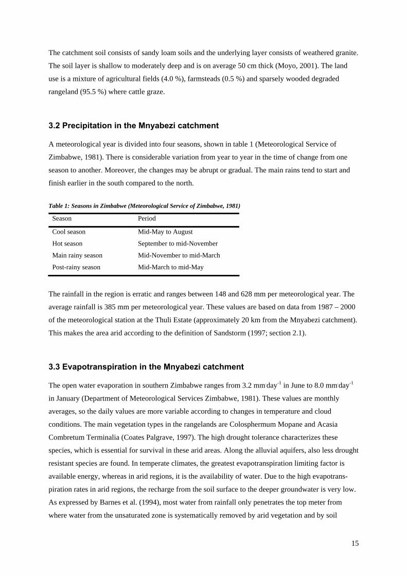
Season Period
Cool season Mid-May to August
Hot season September to mid-November
Main rainy season Mid-November to mid-March
Post-rainy season Mid-March to mid-May
The rainfall in the region is erratic and ranges between 148 and 628 mm per meteorological year. The
average rainfall is 385 mm per meteorological year. These values are based on data from 1987 – 2000
of the meteorological station at the Thuli Estate (approximately 20 km from the Mnyabezi catchment).
This makes the area arid according to the definition of Sandstorm (1997; section 2.1).
3.3 Evapotranspiration in the Mnyabezi catchment
The open water evaporation in southern Zimbabwe ranges from 3.2 mm.day-1 in June to 8.0 mm.day-1
in January (Department of Meteorological Services Zimbabwe, 1981). These values are monthly
averages, so the daily values are more variable according to changes in temperature and cloud
conditions. The main vegetation types in the rangelands are Colosphermum Mopane and Acasia
Combretum Terminalia (Coates Palgrave, 1997). The high drought tolerance characterizes these
species, which is essential for survival in these arid areas. Along the alluvial aquifers, also less drought
resistant species are found. In temperate climates, the greatest evapotranspiration limiting factor is
available energy, whereas in arid regions, it is the availability of water. Due to the high evapotrans-
piration rates in arid regions, the recharge from the soil surface to the deeper groundwater is very low.
As expressed by Barnes et al. (1994), most water from rainfall only penetrates the top meter from
where water from the unsaturated zone is systematically removed by arid vegetation and by soil

16
evaporation following capillary rise. Seepage to groundwater is localised to places where rainwater
concentrates, for example in streambeds and in reservoirs (Sandstrom, 1997). Nevertheless, high
transpiration rates (actual equals potential evapotranspiration) can develop in riparian zones where
water supply is plentiful, for example in alluvial aquifers (Graf, 1988).
3.4 Hydrogeological characteristics of the Mnyabezi catchment
The main water use of the nearly silted reservoir is by drinking of cattle (see figure 8). The local
community is planning to build a new spillway. The difference in maximum water level from the
bottom of the reservoir until the top of the spillway is 0.73 m (for the new spillway it is 1.00 m). When
the reservoir is full it covers an area of approximately 1.54 ha and reaches a total volume of 5600 m3.
The reservoir dries up during long periods of drought. In this period, people can still gain water from
the alluvial aquifer downstream of the dam for a couple of months. Two pumping wells are located
just upstream and downstream from the dam, which are used for domestic purposes and some
gardening. The groundwater level is approximately 4.0 m deep.
Figure 7: Alluvial aquifer of the Mnyabezi River Figure 8: Reservoir of the Mnyabezi River
The Mnyabezi River is highly ephemeral, which means it only flows after a heavy rain event. The
alluvial aquifer downstream of the dam (see figure 7) has a width of approximately 10 meter, an
average depth of 0.9 m and the slope is 0.28 %. The suggested silt or clay layer at the base of the
aquifer by Davis et al. (1995) is not observed in the alluvial aquifer of the Mnyabezi River. The
physical probing done during the field visits only indicate some locally thin clay layers at several
depths, but the main material is fine to medium sand. The underlying granite layer has optimum
weathering conditions. The vegetation along the aquifer is very drought resistant and is not directly
dependent on the water table from the alluvial aquifer itself, because the alluvial aquifer dries out
within a month.
17
4. Method
This chapter describes the methods used in this research. The first section explains the calculation of
the potential water supply. The second and third sections describe the modelling process. The fourth
section explains the measuring strategy for all the parameters and variables. The last section explains
the calibration process of the models.
4.1 Calculation potential water supply
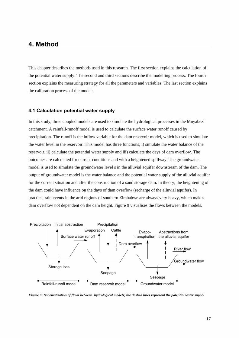
In this study, three coupled models are used to simulate the hydrological processes in the Mnyabezi
catchment. A rainfall-runoff model is used to calculate the surface water runoff caused by
precipitation. The runoff is the inflow variable for the dam reservoir model, which is used to simulate
the water level in the reservoir. This model has three functions; i) simulate the water balance of the
reservoir, ii) calculate the potential water supply and iii) calculate the days of dam overflow. The
outcomes are calculated for current conditions and with a heightened spillway. The groundwater
model is used to simulate the groundwater level s in the alluvial aquifer downstream of the dam. The
output of groundwater model is the water balance and the potential water supply of the alluvial aquifer
for the current situation and after the construction of a sand storage dam. In theory, the heightening of
the dam could have influence on the days of dam overflow (recharge of the alluvial aquifer). In
practice, rain events in the arid regions of southern Zimbabwe are always very heavy, which makes
dam overflow not dependent on the dam height. Figure 9 visualises the flows between the models.
Precipitation
Surface water runoff
Dam overflow
Seepage
River flow
Seepage
Evaporation Evapo-transpiration
Rainfall-runoff model Dam reservoir model Groundwater model
Abstractions from the alluvial aquifer
Cattle
Storage loss
Initial abstraction Precipitation
Groundwater flow
Figure 9: Schematization of flows between hydrological models; the dashed lines represent the potential water supply
18
Because of the sluggishness of the groundwater system, groundwater models usually use a monthly
time step (Sophocleous & Perkins, 2000). However, the alluvial aquifers in the arid regions recharge
relatively fast to normal conditions (Gorgens & Boroto, 1997; Moyce et al., 2006). Furthermore, the
Mnyabezi River is highly ephemeral and thus only flows during and a short period after a rainfall
event. These short hydrological processes require at least a daily time step for the modelling process.
A daily modelling step requires daily input data as well, which has been collected between March
2007 until May 2007.
Every year the dispersion of rainfall events and the amount of rainfall differs. Consequently, the
potential water supply differs for each year as well. The focus of the study is to calculate the potential
water supply and the period of drought during a typical dry, normal and wet year. Note that in arid
regions, the dispersion of rainfall events during a year mainly determines if a year will be typified as
dry, moderate or wet. A period starting at the beginning of the main rainy season (1st of November)
until the end of the hot season (31st of October) is used to make a year simulation. Three typical years
are selected from the daily rainfall records of the Thuli Estate meteorological station between 1987
and 2000. A typical dry year was ‘88/’89 (259.2 mm), a normal year was ‘97/’98 (331.9 mm) and wet
year was ‘96/’97 (568.4 mm).
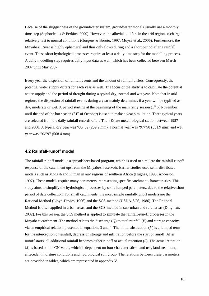
4.2 Rainfall-runoff model
The rainfall-runoff model is a spreadsheet-based program, which is used to simulate the rainfall-runoff
response of the catchment upstream the Mnyabezi reservoir. Earlier studies used semi-distributed
models such as Monash and Pitman in arid regions of southern Africa (Hughes, 1995; Anderson,
1997). These models require many parameters, representing specific catchment characteristics. This
study aims to simplify the hydrological processes by some lumped parameters, due to the relative short
period of data collection. For small catchments, the most simple rainfall-runoff models are the
Rational Method (Lloyd-Davies, 1906) and the SCS-method (USDA-SCS, 1986). The Rational
Method is often applied in urban areas, and the SCS-method in sub-urban and rural areas (Dingman,
2002). For this reason, the SCS method is applied to simulate the rainfall-runoff processes in the
Mnyabezi catchment. The method relates the discharge (Q) to total rainfall (P) and storage capacity
via an empirical relation, presented in equations 3 and 4. The initial abstraction (Ia) is a lumped term
for the interception of rainfall, depression storage and infiltration before the start of runoff. After
runoff starts, all additional rainfall becomes either runoff or actual retention (S). The actual retention
(S) is based on the CN-value, which is dependent on four characteristics: land use, land treatment,
antecedent moisture conditions and hydrological soil group. The relations between these parameters
are provided in tables, which are represented in appendix V.

19
SIP
IPQ
a
a
+−−
=2)(
(3)
25425400−=
CNS (4)
Where ,
Q [mm.day-1] is the runoff,
Ia is the initial abstraction,
S [mm.day-1] is the actual retention,
P [mm.day-1] is the precipitation and
CN [-] is the curve number.
4.3 Reservoir model
The spreadsheet-based model directly couples the dam reservoir model and the rainfall-runoff model.
The runoff from the Mnyabezi catchment, which is calculated by the SCS-method, forms the inflow
variable for the reservoir model. The model also incorporates the variables direct recharge by
precipitation, open water evaporation and abstraction by cattle to calculate the water level in the
reservoir. Groundwater flow into the reservoir is negligible, because the groundwater table in the
underlying granite layer is relatively deep (approximately 4.0 m deep). The model does not simulate
pump abstractions by people from this deeper aquifer. It was not possible to measure the seepage loss
from the reservoir directly, which is the reason the seepage is used as a fitting parameter during the
calibration process.
Besides the determination of the water balance during a dry, normal and wet year, the reservoir model
is also used to calculate the potential water supply and the days of dam overflow for the current
situation and the situation with a heightened spillway. The potential water supply is the summation of
the amount of water that cattle could consume from the reservoir. Dam overflow occurs when the
water level in the reservoir is higher than the height of the spillway.
4.4 Groundwater model
The finite difference ground water model MODFLOW (McDonald and Harbaugh 1988; Harbaugh,
2005) divides the alluvial aquifer system into smaller units supposed to be homogeneous in terms of
their physical characteristics. Based on this distributed character and the relative small spatial scale of
the water system, Visual MODFLOW 4.2 is considered most suitable to simulate the hydrological
processes in the alluvial aquifer.

20
The model consists of three layers (see appendix I). The grid is 230 m in width and 1000 m in length
with a horizontal resolution of 5x5 m. The horizontal resolution of the grid, representing the alluvial
aquifer and the riverbanks (width 10 m each), has a higher resolution of 2x5 m. The alluvial aquifer is
modelled as a rectangular shape with a depth of 0.9 m, a width of 10 m and a slope of 0.28 %. The top
layer (0.7 m) represents the soil, the second layer represents the alluvial aquifer and the lowest layer
the granite. In the MODFLOW model, hydrogeological characteristics, like hydraulic conductivity,
specific yield and porosity, have to be assigned to every layer seperately. Due to the loose
characteristic of the alluvial material, the hydrogeological parameters are assumed to be constant in all
directions. This is not true for granite due to its complex rock structure. Normally, fresh granite has a
very low primary porosity, but granite always has a secondary porosity due to weathering and an
interconnected system of fractures, fissures and joints, which allows the flow and storage of
groundwater. Due to this secondary porosity the hydraulic conductivity, porosity and specific yield of
granite are non-homogeneous. Nevertheless, MODFLOW calculates with average values. Due to the
lack of a good measuring method to determine the value of the hydrolgeological parameters of the
granite layer, these parameters are changed during the calibration process to make a best fit.
The head difference between the water level in the granite layer and the surface level of the alluvial
aquifer is assumed to be constant over the entire length and is used as the initial water head in the
MODFLOW model. At the up- and downstream side, a general head boundary condition is used to
model the groundwater outflow. The RIVER-package is used to model the recharge from the river to
the alluvial aquifer, assuming a constant water level of 1 cm above the riverbed. The streambed
conductance is set high (200 m2.day-1), which allows the aquifer to recharge completely within one
day, like in the natural situation. Direct recharge by precipitation is modelled with the RECHARGE-
package, which directly assigns the amount of recharge to the groundwater table. Overland flow due to
recharge cannot be simulated in MODFLOW model. This is no problem, because most rain events in
arid regions are or very small (negligible overland flow) or very heavy (cause dam overflow, in which
case the alluvial aquifer saturates anyway). In the MODFLOW model evapotranspiration can only be
assigned to the top-layer. The MODFLOW model simulates evapotranspiration with a linear relation
between the user defined maximum rate at the surface of the top-layer and zero evapotranspiration at
the user-defined ‘extinction depth’. Wipplinger (1958) has measured that the evaporation depth from
alluvial aquifers in the arid regions of Botswana is 0.9 m. Borst and DeHaas (2006) found similar
results for a small alluvial aquifer in Kenia. The evapotranspiration of the riparian vegetation is
modelled by multiplying the potential evaporation rate by the crop coefficient and by enlarging the
evaporation depth (equal to the root depth) for the riverbanks. It is assumed that the effective root
depth of the riparian vegetation reaches to the bottom of the alluvial aquifer (1.6 m from the surface).

21
The potential water supply of the alluvial aquifer is calculated for the current situation and the
situation with a sand storage dam. The potential water supply is the summation of daily domestic use
during the period of water storage. The daily abstraction is equal to the domestic use and the water
needed to maintain 10 gardens of 100 m2. The sand storage dam is simulated by the WALL-package,
which uses an impermeable row of cells perpendicular to the alluvial aquifer. The maximum height of
the dam equals the height of the riverbanks at that point. The thickness of the alluvial aquifer is
increased upstream of the dam until the maximum height of the dam, which causes an upstream
influence of 200 m. When in the natural situation the tap in the sand storage dam opens (see figure 5),
the water flows out of the dam with drains situated just above the impermeable underlying ground
layer. A 200 m drain, using the DRAIN-package, is used to simulate this process in the MODFLOW
model. Since the drainage capacity depends on the height of the groundwater level, the drain
conductance [m2.day-1] has to be adjusted to regulate a constant daily discharge. Sand storage dams are
normally built on top of a rock layer with a very low permeability. Since the underlying layer of the
Mnyabezi catchment consists of heavily weathered granite, the seepage loss is large. To make sure
that the sand storage dam has effect in this particular situation, a layer with a low permeability (for
example clay) is modelled at the bottom.
4.5 Measuring strategy
This section discusses the measuring methods of the parameters and variables. Data acquisition is
necessary to acquire direct quantitative information from the Mnyabezi catchment. Some weeks has
been spent doing on-site field measurements in Zimbabwe, while two field assistants measured the
hydrological variables every day. Two catchments have been observed during the measuring period;
the Mnyabezi catchment itself and the Bengu catchment. The extra data from the Bengu catchment
gives the opportunity to calibrate the rainfall-runoff and reservoir models better. The Bengu catchment
covers 8 km2, is located next to the Mnyabezi catchment and has similar hydro(geo)logical
characteristics. The measurements in the alluvial aquifer have only been done for the Mnaybezi
catchment, because the alluvial aquifer of Bengu River is to small to sustain a substantial amount of
water in the sands.
By working with the models insight was obtained into the sensitivity of parameters and variables
before the measurements started. The results of the sensitivity analyses are presented in sections 6.2
and 6.4. The analyses are performed by recording the change in output [%] after changing an input
value [%] of certain parameter or variable, while keeping the other parameters and variables constant.
The parameters and variables with a high sensitivity value required more attention to determine than
those with a low sensitivity.

22
Tables 2, 3 and 4 provide an overview of the methods, locations and frequencies for all the measured
parameters and variables in the Mnyabezi catchment. In the Bengu catchment the same measurements
are conducted to determine the parameters and variables used in rainfall-runoff and the reservoir
models.
Table 2: Measuring strategy parameters and variables rainfall-runoff model
Parameter Measuring Method Location Frequency
Precipitation rate [mm.day-1]
7 standard rain gauges
Documents
Distributed over the catchment
Thuli Estate meteorological Station
Daily at 8 a.m.
Daily; in the period from
1987 – 2000
Area catchment Topographical map - Once
Hydrological soil group Sieving test 3 ground samples of soil Once
Land use catchment area [ha] Survey with GPS
Topographical map
Upper-Mnyabezi catchment Once
Land treatment Observation field Upper-Mnyabezi catchment Once
Hydrological condition Observation field
Satellite image
Upper-Mnyabezi catchment Once
Initial abstraction [%] Calibration - -
Table 3: Measuring strategy parameters and variables reservoir model
Parameter Measuring Method Location Frequency
River inflow Rainfall-runoff model - -
Water level reservoir [mm] Gauging plate In the reservoir Daily at 9 a.m.
Evaporation rate [mm.day-1] American class A Pan
Documents
Pan at Bengu School
Beitbridge metrological station
Daily at 8 a.m.
Monthly (average); in the
period from 1935 - 1980
Profile of the reservoir [m3] GPS-device
Dumpy level
Points where the height of the
reservoir equals the spillway height
Once
Height spillway [m] Dumpy level Spillway Once
Abstractions cattle [m3.day-1] Survey farmsteads in
the surroundings
Number of cattle in the surroundings
of the dam
Once
Water use livestock unit [l.day-1] Literature - -
Seepage [mm.day-1] Calibration - -
Table 4: Measuring strategy parameters en variables MODFLOW model
Parameter Measuring Method Location Time scale
Days of river flow Reservoir model - -
Hydraulic head in alluvial aquifer [m] 8 piezometers 4 perpendicular lines along the aquifer
every 250 m downstream of the dam
Daily at 9 a.m.
Hydraulic head in granite layer [m] Dip-measure Wells up-and downstream of the dam Monthly
Potential Evapotranspiration rate
[mm.day-1]
Documents
Penman equation
Beitbridge metrological station
Monthly (average); in the
period from 1935 - 1980
Crop coefficient Literature - -
Evaporation depth Literature - -

23
Domestic use people [m3.day-1] Survey farmsteads in
the surroundings
Amount of water used per day per
farmstead
Average of 5 days
Water use people to maintain a garden
for personal use [m3.day-1]
Survey farmsteads in
the surroundings
Water used to maintain a garden near
the pump.
Average of 10 gardens
Profile of the aquifer [m] Physical probing
Resistivity test
4 perpendicular lines along the aquifer Once
Slope riverbed [%] Dumpy-level
Tape-line
In the riverbed Once
Streambed conductance Literature - -
Hydraulic conductivity of the alluvial
aquifer [m.day-1]
Sieving test
Permeability test
Slug test
6 samples alluvial material (in lab)
60 dm3 of alluvial material (in lab)
In the alluvial aquifer itself (in situ)
Once
Once
Once
Hydraulic conductivity of the soil
[m.day-1]
Sieving test
Literature
3 ground samples of the soil Once
Porosity [-] for the alluvial material
and the soil layer
Porosity test for alluvial
material and soil
6 ground samples of alluvial material
and the 2 ground samples of soil
Once
Specific yield [-] for the alluvial
material and the soil layer
Literature - -
Hydraulic conductivity [m.day-1],
specific yield [-] and porosity [-] of
the underlying granite
Calibration - -
Most parameters and variables mentioned in the previous tables are determined with straightforward
hydro(geo)logical methods and need no extra explanation. The only methods that need some
explanation are those determining the hydraulic conductivity of the alluvial material. Since this
parameter depends on the grain size distribution and structure of the alluvial material, the value can
differ per area. According to Wipplinger (1958) the composition of sands in an alluvial aquifer
generally shifts from fine sands at the top, medium sands in the middle to coarse sand at the bottom.
Sieving tests have been conducted to determine the grain size distribution of the alluvial material
(samples were taken from the mid-section of the alluvial aquifer). Shephard (1989) developed a
commonly used equation, which relates the grain size and the hydraulic conductivity. He found
equation 5, which represents the relation for alluvial deposits.
65.1
5050 450 dCdK j ⋅== (5)
Where,
K [ft.day-1] is the hydraulic conductivity,
d50 [mm] is the mean grain size,
C [-] is the shape factor and
j is an exponent.

24
Supplementary to the sieving test, a slug test and a permeability test have been conducted to measure
the vertical hydraulic conductivity. Darcy’s law is the basis for these tests (see respectively equations
6 and 7). Figures 10 and 11 visualize the tests schematically. The tests work with a vertical slope (i =
1). For the slug test a pvc-tube has been used with a length of 1.00 m and a diameter of 0.07 m
representing a vertical water column. The tube has been dug into the alluvial aquifer 19 cm under the
groundwater level. Sluts has been made within the reach of the groundwater level and the end of the
tube was closed (H = 0.165 m and h = 0.835; first slut have been made 0.025 m above the bottom of
the tube). Next, water has been poured into the pvc-tube until the top. A stopwatch measured the time
needed to attain the initial water level.
HdThd
AQK
iKiA
QK
z⋅⋅⋅⋅
==⎪⎭
⎪⎬⎫
=⋅
=π
π /))5.0((
1:
2
(6)
2)5.0(/
1: dTV
AQK
iKiA
QK
z⋅
==⎪⎭
⎪⎬⎫
=⋅
=π
(7)
Where,
K [m.day-1] is the hydraulic conductivity, A1 [m2] is the cross-sectional area of the sample,
Q [m3.day-1] is the flow rate, T [day] is the time,
i [-] is the slope, d[m] is the diameter of the sample and
h [m] is the head difference V [m3] is the volume of percolated water
h
H
d
Inflow
V
Overflow
d Figure 10: Schematization of the slug test Figure 11: Schematization of the permeameter test
For the permeability test a bucket with a volume of 60 dm3 has been filled until the top with alluvial
material (dtop = 0.48 m, dbottum = 0.41 m, h = 0.40 m). A continual inflow of water held the hydraulic
head constant. The outlet at the bottom of the bucket was 25 mm in diameter. A coarse gravel filter
placed at the outlet prevented sediment flowing out of the bucket. A stopwatch measured the time
needed to fill another 5 dm3 bucket.
25
4.6 Calibration method
It is desirable that models reflect the physical reality as closely as possible. In a calibration process,
some parameters are varied to make a best fit between the measured and equivalent simulated values
(Hill, 1998). Three calibration approaches are commonly used; manual calibration, automatic
calibration and Monte Carlo simulations. In this research a manual calibration is conducted, since it
provides most insight into the behaviour of models. To reduce subjectivity in fitting models, it is
necessary to use an index of agreement or disagreement between the observed and simulated results
(Weglarczyk, 1998). Nash & Sutcliffe (1970) developed one of the most used methods for
hydrological purposes, i.e. the efficiency coefficient represented by equation 8. As a “rule of thump”,
it can be said that the model performs reasonably well when values between 0.6 and 0.8 are obtained.
Values between 0.8 and 0.9 indicate that the model performs very well and values between 0.9 and 1.0
indicate that the model performs extremely well.
∑
∑
=
=
−
−−= N
ii
N
iii
OO
POE
1
2
1
2
)(
)(1 (8)
Where, E [-] is the efficiency coefficient, O [-] are the observed values andP [-] are the predicted values.
The efficiency coefficient is used to judge on the rainfall-runoff and reservoir model, using the
observed and calculated water levels of the Mnyabezi and Bengu reservoirs. Since the Mnyabezi and
Bengu rivers are ungauged, it is necessary to calibrate the rainfall-runoff model in combination with
the reservoir model. Figure 12 shows this relation between both models during the calibration process.
By knowing the increase in water level of the reservoir after a rain event, the amount of river inflow is
calculated. This value is used to calibrate the rainfall-runoff model. For the rainfall runoff model the
initial abstraction is used as the fitting parameter for the calibration of the model. The initial
abstraction is difficult to determine in arid regions due to surface crust forming (FAO, 1991) and the
high transmission losses into the alluvial aquifer (Anderson, 1997). These features make the normal
assumption of Ia = 0.2.S (Soil Conservation Service, 1972) not valid. Studies in southern Africa have
used percentages of 10 % and less (Schulze et al., 1993; Hranova, 2006). To obtain the best fit, the
initial abstraction is changed between 5.0 and 15.0 % of actual retention S. For the reservoir model the
seepage is used as the fitting parameters for the calibration of the model, due to the lack of a good
method to determine this parameter. The seepage is assumed less than the open water evaporation and
has been varied between 0.0 and 1.0 mm.day-1.

26
Land-use
CN-values [-] Storage [mm.day-1]
Precipitation [mm.day-1] Discharge
River [m3.day-1]
Evaporation from reservoir
[m3.day-1]Evaporation [mm.day-1]
Area catchment
[m2]
Pricipitation P[m3.day-1]
Surface area reservoir [m2]
Abstractions by cattle [m3.day-1]
Cattle drinking from reservoir
[#.day-1]
Water use per life stock unit
[m3]
Calculated water level
reservoir [m]
Days of dam overflow [m3.day-1]
Seepage [m3.day-1]
Precipitation [mm.day-1]
Surface of the reservoir [m2]
Dimensions of the reservoir
[m-m-m]
Fitting parameter/variable for calibration
Input parameter/variable
Calculated parameter/variable
Output parameter/variable
Variable used for calibration
Antecedent moisture
conditions
Hydrological soil group
Initial abstraction [% storage]
Hydrological condition
Rainfall-runoff model
Reservoir model
Seepage [mm.day-1]
Height spillway [m]
Land treatment
Figure 12: Relation between parameters and variables for the rainfall-runoff and reservoir models
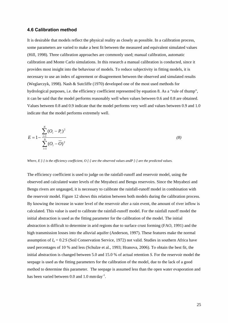
In the MODFLOW model the observed and calculated groundwater level in the alluvial aquifer are
used to calibrate the model. Figure 13 shows the relation between the parameters and variables during
the calibration process. The MODFLOW model calculates automatically a correlation coefficient after
importing ‘observation wells’. The underlying granite layer consists of rock with heavy weathering
conditions. Due to the lack of a good method to determine the values for the hydraulic conductivity,
specific yield and effective porosity for the granite layer, these parameters are used as fitting
parameters for the calibration of the model. The hydraulic conductivity for weathered granite ranges
between 0.5 – 1.4 m.day-1 (Morris & Johnson, 1967; Davis, 1969; Shaw, 1994). The specific yield for
weathered granite ranges between 0.01 and 0.05 and the effective porosity ranges between 0.05 and
0.15 (Todd, 1980; Rushton & Weller, 1989). The hydraulic conductivity and the specific yield were
manually varied between the above ranges to make a best fit. Since the sensitivity of the porosity was
low, this value was assumed constant at a value 0.08. After the manual calibration, the PEST-module
of the MODFLOW model fine-tuned the calibration automatically.
27
Days of dam overflow [m3.day-1]
Boundary head in- and
outflow [m3.day-1]
Slope [m/m]
Evaporation depth [m]
evapotranspiration [m3.day-1]
Recharge aquifer
[m3.day-1]
Streambed conductance
[m2.day-1]
Fitting parameter for calibration
Input parameter/variable
Calculated parameter/variable
Output parameter/variable
Water table depth [m]
Porosity, specific yield and hydraulic conductivity aquifer [-]
Porosity, specific yield and hydraulic conductivity
soil [-]
Dimensions ground layers
[m3]Hydrogeological characteristics ground layers
Abstraction [m3.day-1]
Variable used for calibration
Porosity, specific yield and hydraulic conductivity granite [-]
Surface area aquifer [m2]
Crop coefficient
Open water evaporation [mm.day-1]
Surface area river bank [m2]
Figure 13: Relation between parameters and variables for the groundwater model

28
5. Results field measurements
This chapter presents the results of the field measurements. The first section describes the field
measurement results of the rainfall-runoff model. The second section provides the results for the
reservoir model. At last, the results for the groundwater model are presented
5.1 Rainfall-runoff model
This section provides the results for the parameters and variables used in the rainfall-runoff model.
The first sub-section describes the determination of the hydrological soil group. The second sub-
section discusses the average CN-value and the last the rainfall records.
5.1.1 Hydrological soil group
According to Moyo (2001), who has done soil analysis in the Fumukwe catchment (10 km away from
the Mnyabezi catchment), soils in the area are well drained and consist of loamy sand. The results of
the sieving tests for the Mnyabezi catchment provide similar results (see table 5; appendix XIII).
According to Maidment (1992), soils consisting of loamy sand result in hydrological soil group “A”.
Table 5: Comparison results grain size analysis soil (* estimates; total is 11 %)
Fumukwe catchment Mnyabezi catchment
Clay 7 % 7 %*
Silt 3 % 4 %*
Fine sand 36 % 35 %
Medium sand 27 % 31 %
Coarse sand 20 % 20 %
Gravel 8 % 3 %
Soil type (USDA classification) Loamy sand Loamy sand
Soil type (BSI) Fine sand Fine sand
Appendix VI presents hydraulic conductivities for several soil textures. The average K-value for
loamy sand is 13.48 m.day-1 (Dingmans, 2002), which is used for the hydraulic conductivity of the soil
in the MODFLOW model.

29
5.1.2 Average CN-value
The Thiessen polygons divide the Mnyabezi catchments into seven polygons (each rain gauge
representing one polygon). For each polygon, a specific CN-value is calculated based on the land-use,
land treatment, hydrological condition and antecedent moisture conditions. A field survey has been
done to map the land use (see appendix III). Appendix IV presents the results for the Bengu
catchment. The rangelands are classified as “pasture lands”. The hydrological condition depends on
the intensity of grazing activities and vegetation coverage (see appendix II). In general, there is much
activity near the reservoir (poor condition), which decreases upstream (good condition). The
agricultural fields are classified as “row crops” in poor hydrological conditions, because the maize is
planted in rows far enough apart that most of the soil surface is directly exposed to rainfall. Table 6
presents the average curve numbers per polygon for the Mnyabezi catchment with normal antecedent
moisture condition. The rainfall-runoff model calculates automatically the antecedent moisture
conditions based on the amount of rainfall in the preceding five days.
Table 6: CN-value of the Thiessen polygons for the Mnyabezi catchment
Polygon Area [ha] Rangeland [%] fields [%] Farmsteads [%] Hydrological
condition
CN-value [-]
1 20 90 0 10 (2 farms) Poor 67.1
2 50 88 2 10 (5 farms) Poor 67.2
3 220 75 20 5 (5 farms) Fair 54.1
4 150 80 18 2 (3 farms) Fair 53.3
5 350 97 3 0 Fair 49.7
6 400 100 0 0 Good 39.0
7 1010 100 0 0 Good 39.0
5.1.3 Rainfall-events
It was extremely dry in southern Zimbabwe during the measuring period, which was caused by El
Niño effects (FewsNet, 2006). Due to this drought, only three major rain events occurred; on the 26th
of February (20 – 40 mm), on the 29th of March (40 – 70 mm) and on the 5th of April (2.5 – 30 mm).
The effects on the water level in the reservoir of the first rain event has not been recorded with
gauging plates, because they had not been installed yet. However, the field assistant for the Bengu
reservoir recorded a water level heightening from nearly dry to approximately 50 cm on the 26th of
February. The heavy rain event of the 29th of March was followed by dam overflow at both
catchments. The rainfall event on the 5th of April only lead to water level rise in the Mnyabezi
reservoir. Appendix VII presents the rough precipitation records. Figure 14 shows the effects of the
rainfall on the water level in both reservoirs.

30
5.2 Reservoir model
This section provides the results for the parameters and variables used in the reservoir model. The
variables are described in the first sub-section and the parameters in the second sub-section.
5.2.1 Variables concerning the water level in the reservoir
Figure 14 presents the water level of the Mnyabezi and Bengu reservoirs, which has been measured
with gauging plates in the reservoir. As stated in sub-section 5.1.3 a heavy rain event occurred on the
29th of March. The figure shows clearly the dam overflow events in both reservoirs, caused by this rain
event. The open water evaporation, measured with a standard American A pan, is on average 6.1
mm.day-1 (s.d. = 2.5 mm.day-1) in March and 5.0 mm.day-1 (s.d. = 1.8 mm.day-) in April 2007. The
open water evaporation at Beitbridge meteorological station for these months, which are based on data
from 1935 – 1980, are respectively 6.4 mm.day-1 and 5.0 mm.day-1 (see table 8). Thus, the recorded
pan evaporation at Bengu are comparable to the evaporation records of this meteorological station.
The abstractions by cattle from the reservoir, determined by a field survey, are 11.6 m3.day-1 for the
Mnyabezi reservoir and 31.8 m3.day-1 for the Bengu catchment. Appendices VIII to XI present all the
rough data for the precipitation, open water evaporation and abstraction by cattle.
0
10
20
30
40
50
60
70
80
90
10-03-07 17-03-07 24-03-07 31-03-07 07-04-07 14-04-07 21-04-07 28-04-07 05-05-07
Date [dd-mm-yy]
Wat
er le
vel r
eser
voir
[cm
]
Water level Mnyabezi
Spillway Mnyabezi
Water level Bengu
Spillway Bengu
Figure 14: Water level Mnyabezi and Bengu reservoirs
Appendix XII provides the results of the survey done to determine the total domestic water use from
the people in the surroundings of the Mnyabezi reservoir dam (3.6 m3.day-1) and the amount of water
needed to maintain one garden of 100 m2 (0.35 m3.day-1).
5.2.2 Dimensions of the reservoir
The dimensions of the reservoir have been determined by a GPS-device and a dumpy level. Points
have been marked for the Mnyabezi and Bengu reservoir where the height of the surface area equalled
the height of the spillway, which resulted in the maximum supply level of both reservoirs (see table 7).
After consult from a water engineer of ZINWA (Zimbabwe Water Authority), a 1.00 m height of the
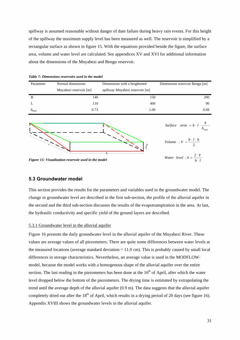
31
spillway is assumed reasonable without danger of dam failure during heavy rain events. For this height
of the spillway the maximum supply level has been measured as well. The reservoir is simplified by a
rectangular surface as shown in figure 15. With the equations provided beside the figure, the surface
area, volume and water level are calculated. See appendices XV and XVI for additional information
about the dimensions of the Mnyabezi and Bengu reservoir.
Table 7: Dimensions reservoirs used in the model
Parameter Normal dimensions
Mnyabezi reservoir [m]
Dimensions with a heightened
spillway Mnyabezi reservoir [m]
Dimensions reservoir Bengu [m]
B 140 150 200
L 110 400 90
hmax 0.73 1.00 0.69
b
l hm
ax
Figure 15: Visualization reservoir used in the model
5.3 Groundwater model
This section provides the results for the parameters and variables used in the groundwater model. The
change in groundwater level are described in the first sub-section, the profile of the alluvial aquifer in
the second and the third sub-section discusses the results of the evapotranspiration in the area. At last,
the hydraulic conductivity and specific yield of the ground layers are described.
5.3.1 Groundwater level in the alluvial aquifer
Figure 16 presents the daily groundwater level in the alluvial aquifer of the Mnyabezi River. These
values are average values of all piezometers. There are quite some differences between water levels at
the measured locations (average standard deviation = 11.0 cm). This is probably caused by small local
differences in storage characteristics. Nevertheless, an average value is used in the MODFLOW-
model, because the model works with a homogenous shape of the alluvial aquifer over the entire
section. The last reading in the piezometers has been done at the 16th of April, after which the water
level dropped below the bottom of the piezometers. The drying time is estimated by extrapolating the
trend until the average depth of the alluvial aquifer (0.9 m). The data suggests that the alluvial aquifer
completely dried out after the 18th of April, which results in a drying period of 20 days (see figure 16).
Appendix XVIII shows the groundwater levels in the alluvial aquifer.
lbVhlevelWater
hlbVVolume
hhlbareaSurface
⋅⋅
=
⋅⋅=
⋅⋅=
2:
2:
max

32
Figure 16: Groundwater level in the alluvial aquifer; measured from the surface area (average values over the
piezometers; s.d. = 11.0 cm)
The initial water level in the granite layer is 3.9 m beneath the surface of the alluvial aquifer, which
has been measured with a dip measure in the water pumps.
5.3.2 Profile of the ground layers
The width of the alluvial aquifer has been measured with a tapeline. The depth of the alluvial aquifer
has been measured at four rectangular lines by physical probing. A weathered granite layer underlies
the river, so it was easy to determine the depth manually with an iron rod. Appendix XVII shows the
results of the physical probing of the aquifer. The average width in the first 1.0 km downstream of the
dam ranges between 9.0 and 10.5 m. The maximum depth is 1.30 m with an average of 0.91 m. The
thickness of the soil layer, observed at the riverbed of the alluvial aquifer, is estimated between 0.5
and 0.8 m.
Figure 17: Measuring the height with a dumpy level Figure 18: Resistivity test in the alluvial aquifer
Supplementary to the physical probing, direct current electronical resistivity tests has been done to
determine the thickness and hydrogeological characteristics of the underlying granite layer (see figure
18). In earlier studies, resistivity tests gave valuable results for the Mzingwane River and Shangani

33
River in Zimbabwe (Beckman & Liberg, 1997; Owen & Dahlin, 2005). The sand of the alluvial
aquifer has a high resistivity signature and this made it relatively easy to distinguish from underlying
bedrock (Owen & Dahlin, 2005). After analysing the results, the measurements for only two lines gave
reasonable results. Based on the recorded data it is possible to distinguish two ranges of resistivity
values, one representing the alluvial material and one the granite. Alluvial material has resistivity
values above 100 Ω.m and has a maximum depth of 2.0 m. The resistivity values for granite ranges
between 40 to 100 Ω.m and has a depth between 2.0 and 15.0 m. This range indicates rock with heavy
weathering conditions and optimum groundwater potential (Mudzingwa, 1998). The resistivity in the
granite remains quite constant for an increasing measuring depth, which indicates that the granite layer
is uniform for at least 15 m.
5.3.3 Potential evapotranspiration for riparian vegetation
The potential evapotranspiration rate (PET0) is the rate of evapotranspiration from a large area covered
by green grass which grows actively, completely shades the ground and which is not short of water
(FAO, 1991). To calculate the evapotranspiration of riparian vegetation (PETt), the PET0 has been
multiplied by a crop coefficient (kc). The crop coefficient for riparian vegetation has been estimated
from similar drought resistant crop vegetation (olives and citrus trees) and is equal to 0.7 (FAO, 1991).
Table 8: Data meteorological station Beitbridge (Metereological Service of Zimbabwe, 1981)
Month Average
temp. [ºC]
Dry bulb
temp. [ºC]
Wet bulb
temp. [ºC]
Wind
[m.s-1]
Sunshine
[h.day-1]
PET0
[mm.day-1]
PETt
[mm.day-1]
ET0
[mm.day-1]
Jan 27.45 24.0 22.0 4.30 7.2 3.34 2.34 7.97
Feb 27.05 22.6 19.6 3.99 7.0 4.22 2.95 7.07
Mar 25.90 24.5 20.5 3.79 7.8 4.62 3.23 6.42
Apr 23.55 22.2 19.4 3.17 8.1 3.91 2.74 4.97
May 19.95 22.7 19.4 2.46 8.9 3.79 2.65 3.81
Jun 16.80 22.4 19.8 2.35 8.5 3.16 2.21 3.17
Jul 16.65 23.4 20.8 2.56 9.1 2.99 2.09 3.58
Aug 19.10 25.4 23.6 3.17 9.6 2.85 2.00 4.74
Sep 22.60 23.4 22.8 4.09 9.6 2.57 1.80 6.63
Oct 25.35 23.8 22.4 4.81 8.8 3.23 2.26 7.52
Nov 26.35 22.4 21.8 4.50 7.1 2.73 1.91 7.43
Dec 26.95 24.0 22.6 4.30 6.7 3.24 2.27 7.58
Table 8 provides monthly data of the meteorological station in Beitbridge, the calculated evapotrans-
piration and the open water evaporation per month. The meteorological station in Beitbridge has
approximately the same height as the Mnyabezi catchment (450 m above sea level and atmospheric
pressure of 96.1 kPa) and is located about 110 km eastwards. According to the Meteorological Service

34
of Zimbabwe (1981), the meteorological conditions from Beitbridge are similar to those in the
Mnyabezi catchment.
5.3.4 Hydraulic conductivity of the alluvial material
The hydraulic conductivity (Kx, Ky and Kz)) of the alluvial material is an important parameter. This
section presents the results of the sieving test, slug test and permeability test. The sieving test results
show a hydraulic conductivity (K-value) of 76.2 m.day-1 for a d50-value of 0.7 mm. However, the d50-
value can vary +/- 0.05 mm, resulting in a range for the hydraulic conductivity between 67.4 and 85.4
m.day-1. Appendix XIV presents the rough data of the sieving tests.
Table 9 shows the results of the slug test. The last four measurements are used to calculate the
hydraulic conductivity. The first two measurements are not taken into account, because here the
equilibrium was not reached yet. The average K-value is 62.2 m.day-1. However, the results are most
sensitive to the diameter of the pvc-tube (7 cm). The uncertainty in thickness of the tube is +/- 3 mm,
which cause a possible range in diameter between 6.7 and 7.3 cm. This results in a hydraulic
conductivity between 59.7 m.day-1 and 65.0 m.day-1. Table 10 shows the results of the permeability
test. The average K-value is 63.6 m.day-1. The results are very sensitive to the average diameter of the
bucket (44.5 cm). Assuming an error of +/- 1.0 cm in average diameter, the hydraulic conductivity
value ranges between 62.0 m.day-1 and 64.9 m.day-1.
To conclude, the average hydraulic conductivities of the three tests do not differ much, although the
uncertainty differs for each test. The average hydraulic conductivity is 62.9 m.day-1. Due to the large
uncertainty in the sieving test results, this value is not taken into account to calculate the average
value. The result is comparable to the value Wipplinger (1958) found for the hydraulic conductivity
(61 m.day-1) for alluvial sands in Namibia.
Table 9: Results slug test Table 10: Results permeability test Test T [s] Q [m3.day-1] K [m.day-1] Test T [s] Q [m3.day-1] K [m.day-1]
1 105 2.56 70.69 1 43.5 9.93 64.07
2 110 2.45 67.48 2 42.4 10.19 65.73
3 119 2.26 62.73 3 45.2 9.56 61.66
4 120 2.24 61.85 4 43.7 9.89 63.78
5 118 2.28 62.90 5 43.5 9.93 64.07
6 121 2.22 61.34 6 44.1 9.80 63.20
7 43.9 9.84 63.49
8 44.4 9.73 62.77

35
5.3.5 Specific yield and porosity
The total porosity n [-] is defined as the portion of pore spaces in a volume of soil (Mainment, 1992;
Shaw, 1994). The specific yield sy [-] describes the volume of water that drains by gravity out of a
ground layer (Mainment, 1992; Shaw, 1994). The value is an indication of an aquifer’s storage
characteristics. Tables are known in literature (see appendix VI), which provide values for the porosity
and specific yield for different soil and rock types. In this study ground sample analysis of the alluvial
material and soils near to the river have been conducted to determine the porosity. Table 11 presents
the porosity results for the alluvial material. According to Dingman (2002), the porosity of alluvial
material (medium sand) ranges from 0.29 to 0.49. Therefore, the value found for the porosity (0.33)
seems to be realistic. When linearly interpolating the values provided by Dingman (2002), the specific
yield in medium sand equals 0.27 (for a porosity of 0.33).
Table 11: Porosity of the alluvial material
Test Weight dried sample
[g]
Weight saturated sample
[g]
Volume water
[ml]
Volume baker
[ml]
Porosity
[-]
1 1008.3 1177.7 169.4 500 0.339
2 976.7 1156.3 179.6 500 0.359
3 698.5 799.2 100.7 300 0.336
4 636.4 732.7 96.3 300 0.321
5 617.8 713.1 95.3 300 0.318
6 668.8 769.9 101.1 300 0.337
Average 0.33
Table 12 presents the porosity results for the soil samples, which has been measured in a baker with a
volume of 500 ml. According to Dingman (2002), the porosity of the soil ranges from 0.29 to 0.53.
Therefore, the calculated value for the porosity (0.37) seems to be realistic. When linearly
interpolating the values presented by Dingman (2002), the specific yield in fine sand equals 0.22 (for a
porosity of 0.37).
Table 12: Porosity of the surface soil
Test Weight dried sample [g] Weight saturated sample [g] Volume water [ml] Porosity [-]
1 1139.0 1327.6 188.6 0.377
2 972.1 1155.6 183.5 0.367
Average 0.37

36
6. Results models
This chapter shows the results of the sensitivity and calibration process. The first two sections
highlight the results for the rainfall-runoff model. The third and fourth sections provide the
MODFLOW model results. The last section discusses the uncertainty in the outcomes.
6.1 Sensitivity of the reservoir and rainfall-runoff models
A sensitivity analysis shows the parameters and variables that mostly contribute to the output
variability. The parameters mentioned in table 2 and 3 are analysed together. This is done by varying
the input values between -20 % and 20 %, while keeping the other parameters and variables constant.
Figure 19 presents the results for the parameters and variables with the largest sensitivity values. The
figure shows clearly that the parameters and variables concerning the rainfall-runoff relation are most
sensitive. The sensitivity of the parameters concerning the reservoir model are less sensitive, except
for the parameter ‘height spillway’.
0
10
20
30
40
50
60
70
-20 -15 -10 -5 0 5 10 15 20
Change in input [%]
Sens
itivi
ty o
utpu
t [%
]
EvaporationHeight spillwayPrecipitationCN-valueInitial abstraction
Figure 19: Sensitivity parameters and variables rainfall runoff model
Precipitation is the only input variable; the output is logically very sensitive to changes in this
variable. The most sensitive parameters are the ‘CN-value’ and the ‘initial abstraction’. The initial
abstraction is a very complex lumped parameter dependent in soil characteristics. The CN-value is
also a lumped parameter, which include land use, land treatment, antecedent moisture conditions and a
hydrological soil group. Since both depend on soil characteristics in the catchment, is it necessary to
investigate the combined sensitivity. Figure 20 shows that the combined sensitivity does not have a
higher sensitivity values than the separate sensitivity values.

37
-15% -7%
-2% 2% 7% 15%
-1 5 %
-7 %
-2 %
2%
7%
15 %
C h a n g e in In it ia l a b s tra c t io n [% ]
Change in
CN
-value [%]
6 0 % -8 0 %
4 0 % -6 0 %
2 0 % -4 0 %
0 % -2 0 %
Figure 20: Sensitivity CN-value and initial abstraction
6.2 Calibration of the reservoir and rainfall-runoff models
As stated in section 4.6, the water level records of the Mnyabezi and Bengu reservoirs are used to
calibrate the models. During the measuring period, three rainfall events occurred; one without dam
overflow on the 26th of February (only recorded for the Bengu reservoir) and one with dam overflow
on the 29th of March (in both reservoirs) and one without dam overflow on the 5th of April (only in the
Mnaybezi reservoir). The effects on the water level in the reservoirs of the first rainfall event have not
been recorded with gauging plates, because they had not been installed yet. However, the field
assistant recorded a water level heightening from nearly 0 cm until approximately 50 cm during this
rain event. Because of this extra information, the calibration process started with the Bengu rainfall-
runoff model. Next, the value found for the initial abstraction [% of actual retention] is used for the
Mnyabezi reservoir model. Hereafter, the seepage [mm.day-1] is used to calibrate the Mnyabezi
reservoir model further and this seepage value is transferred to the Bengu reservoir model. In the
Bengu rainfall-runoff model the initial abstraction is changed again to make an even better fit. This
iterative way gave eventually the optimum values for the initial abstraction and seepage. An efficiency
coefficient of 0.99 is obtained for both models, using an initial abstraction of 7.6% of the actual
retention and seepage of 0.0 mm.day-1. These results are in line with similar studies conducted in arid
regions in southern Africa (Schulze et al., 1993; Hranova, 2006).
During the calibration process, it has been assumed that both reservoirs have equal values for the
initial abstraction and seepage. Since both catchments have the same meteorological conditions, land
use and hydrogeological characteristics, this assumption seems to be justifiable. The graphs in figures
21 and 22 show clearly an increase of water level in both reservoirs after the heavy rain event on the
29th of March. The model does not simulate the water level above the spillway, which gives the
Sensitivity output [%]

38
opportunity to calculate the amount of dam overflow (amount of water inflow after reaching the
spillway height). This can also be seen in the figures, where the observed water levels are higher than
calculated water levels just after the heavy rain event on the 29th of March.
0102030405060708090
10-feb 2-mrt 22-mrt 11-apr 1-mei
Date [dd-mm]
Wat
er le
vel [
cm]
Measuredwater level
Calculatedwater level
Figure 21: Calibration results Bengu reservoir
0102030405060708090
4-mrt 14-mrt 24-mrt 3-apr 13-apr 23-apr 3-mei
Date [dd-mm]
Wat
er le
vel [
cm]
Measuredwater level
Calculatedwater level
Figure 22: Calibration results Mnyabezi reservoir
6.3 Sensitivity of the groundwater model
The sensitivity analysis for the MODFLOW model is not performed as extensively as for the rainfall-
runoff model. The analysis is more qualitatively, based on experiences obtained during the model
building process and the calibration process. The main sensitivity lies within the hydraulic
conductivity and specific yield of the granite layer, which are the fitting parameters during the
calibration process. The porosity has a negligible sensitivity, which makes the assumed constant value
of 0.08 during the calibration process legitimate. The hydraulic conductivities of the alluvial aquifer
and soil layer have a minor influence on the output. Another parameter with a significant influence on
the output is the streambed conductance, which regulates the river leakage into the alluvial aquifer.
This value is chosen in such a way that it exactly recharges the alluvial aquifer during one river flow
event.

39
6.4 Calibration of the groundwater model
In the MODFLOW model, two “head observation wells” (at 100 m and 600 m downstream of the
dam) were imported. These wells compared the groundwater levels measured with piezometers and
the calculated groundwater levels (see figure 23). Hereafter, the MODFLOW model calculated
automatically a correlation coefficient between the observed and calculated values for every run.
During the calibration process the hydraulic conductivity of the granite layer was changed between 0.5
and 1.4 m.day-1 and the specific yield between 0.01 and 0.05 to make the best fit. At the end, the
PEST-module automatically fine-tuned the manual calibration process. A correlation coefficient of
0.99 is obtained using a value of 0.55 m.day-1 for the hydraulic conductivity and 0.03 for the specific
yield.
4.5
5
5.5
6
6.5
7
7.5
0 5 10 15 20 25
Time [days]
Wat
er le
vel f
rom
bot
tom
mod
el [m
]
Calculated water level 600 mdownstream of the damMeasured water level 600 mdownstream of the damCalculated water level 100 mdownstream of the damMeasured water level 100 mdownstream of the dam
Figure 23: Calibration results groundwater model
The MODFLOW model also provides the discrepancy in mass balance results. In general, a
discrepancy between in- and outputs of less than 2% is a good performance of the model (Waterloo
Hydrologic, 2006). The water mass balance resulted in a maximum error of 5.0 % (during the day of
river flow). Hereafter, the river flow discrepancy in mass balance remained within a +/- 1.0 %
boundary.
6.5 Uncertainty in outcomes
Walker et al. (2003) describe uncertainty as “being any deviation from the unachievable ideal of
completely deterministic knowledge of the relevant system”. Due to uncertainty in input data and
relations between parameters and variables, the results used in the models are always subjected to
uncertainty. However, downplaying the usefulness of models by claiming that modelling by definition
denies the essence of uncertainty was not very useful either. A more constructive approach is to
analyse how uncertainty materializes in the catchment modelling (Van Asselt & Rotmans, 2002). Due

40
to a lack of data to verify the outcomes and due to a short measuring period, the uncertainty in
outcomes for the Mnyabezi catchment is high. The main interest for this study lies in the uncertainty
of the measuring and modelling methods, for which a qualitative analysis has been performed.
Walker et al. (2003) provide a framework to describe systematically uncertainties in models, which is
used in this study. Appendix XX presents one framework for every model. The “context uncertainty”
is negligible in all models, because there is no discussion about the boundaries of the hydrological
system. The “technical uncertainty” in the spreadsheet-based models is negligible as well, because the
calculation method does not have errors in water balance outcomes. There is a small “technical
uncertainty” in the groundwater model, because the finite difference model has a small error in water
balance outcomes (+/- 1%). The uncertainty caused by external driving forces that produce changes
within the system, like in influence of climate change, goes outside the scope of this research and is
therefore not relevant in this situation. The natures of all “parameter uncertainties” are epistimetic,
which means that uncertainty can reduce by more research and empirical efforts. The most important
uncertainties for each model are described in more detail below.
The main uncertainty for the rainfall-runoff model lies within the model structure on scenario level. At
this moment, the complex hydrogeological relations are lumped in an equation to calculate the runoff,
linking the parameters CN-value, initial abstraction and the variable precipitation. The CN-value and
initial abstraction, which are sensitive parameters (see figure 19), are assumed to be constant during
the whole year. Nevertheless, the CN-value can vary in time due to change in land use or land
treatment. The initial abstraction can vary in time due to crust forming on the surface or saturation of
the alluvial aquifer. The rainfall-runoff model has only been calibrated on one rainfall event in the
Bengu and Mnyabezi catchment. This causes a large uncertainty in the outcomes of the rainfall-runoff
model. Nevertheless, the drying periods of the reservoirs have been monitored quite well. Since the
main objective of the study is to calculate the potential water supply after the start of main rainy
season (where the reservoir fills up completely anyway), the results still provide useable outcomes.
The main “parameter uncertainty” within the reservoir model, besides the uncertainty in the river
inflow described above, are the dimensions of the reservoir in relation to the water level. The
dimensions of the reservoir have not only influence on the “statistical uncertainty” under normal
circumstances, but on the “scenario uncertainty” (heightening of the spillway) as well. The sensitivity
analysis (see figure 19) also shows a relative high sensitivity of this parameter. At this moment, a
simple rectangular shape simulates the dimensions of the reservoir. This can be improved by
measuring the exact shape of the reservoir with a dumpy level when the reservoir is dry.
In arid regions, heavy rain events are mostly followed by large amounts of dam overflow, which
causes a complete saturation of the alluvial aquifer. In that situation, the uncertainty in amount of dam

41
overflow, caused by the “parameter uncertainty” in the dimensions of the reservoir, has no influence
on the groundwater model outcomes. Only when the dam overflow is very small, which causes the
alluvial aquifer to saturate only partly, the outcomes of the groundwater model are influenced by the
uncertainty in the reservoir model.
One uncertainty in the MODFLOW model structure is the calculation of evapotranspiration from
riparian vegetation. The model has some disadvantages in modelling evapotranspiration. MODFLOW
uses a linear relation for the evapotranspiration, which depends on the groundwater depth from the
top-layer. Since the evapotranspiration highly depends on the water content characteristics of the
unsaturated soil, this is not the most accurate way to model evapotranspiration. The MODFLOW-
SURFACT engine can solve this problem, but than information about pf-curves, water contents in the
unsaturated zone and other soil science parameters are required. The sensitivity analysis results in a
small influence from the evapotranspiration of riparian vegetation on the output (the water level in the
alluvial aquifer). Most of the water evaporated directly from the alluvial aquifer itself, which makes it
possible to work with the current data. Nevertheless, the model restriction causes a little
underestimation of the total evapotranspiration.
Another main uncertainty in the MODFLOW model structure is on scenario level. The calculations for
the sand storage dam are conceptual and the outcomes are not verified with measured data. This
causes a large uncertainty in the relations between seepage, evapotranspiration and abstractions by
users. In continuation of this research, it would be very interesting to monitor the hydrological
processes of a sand storage dam in situ to reduce this uncertainty.

42
7. Analysis
This chapter presents the analysis of the modelling results. The first and second sections provide the
water balance and potential water supply of the rainfall-runoff model. The third and fourth sections
describe the same results for the MODFLOW model. The last section discusses the outcomes of the
models.
7.1 Water balance of the Mnyabezi reservoir
The reservoir model has been used to analyse the hydrological characteristics of the reservoir during a
dry year (‘89/’99), a normal (‘97/’98) and wet year (‘96/’97). Note that in arid regions, the dispersion
of rainfall events during a year mainly determines if a year will be typified as dry, moderate or wet.
The water balance results of the reservoir for these three years are presented in figure 24. The results
show approximately the same proportions between natural losses; the evaporation loss is 79 %, cattle
abstractions count for 21 % and the seepage losses are negligible. Of course, this means that the total
amount of evaporation and abstractions by cattle increases for wetter years in comparison to drier
years. The differences in reservoir inflow are caused by the different rainfall patterns: in dry years, the
rainfall is mainly concentrated during a few heavy rain events and in wetter years, the rain events are
less heavy, but more frequent and better dispersed over a longer period. In drier years all rain events
cause river flow, that directly spills over the dam (99%). In wetter years smaller rain events without
causing river flow occur more frequently, which is the reason the proportion of direct precipitation in
the reservoir is higher.
River inflow [100%]
River inflow Reservoir [1%]
Dam overflow [99%]
P [43%]River inflow
Reservoir [57%]
E [79%] Cattle [21%]
Seepage [0%]Dry year
River inflow [100%]
River inflow Reservoir [1%]
Dam overflow [99%]
P [55%]River inflow
Reservoir [45%]
E [78%] Cattle [22%]
Seepage [0%]Normal year
River inflow [100%]
River inflow Reservoir [3%]
Dam overflow [97%]
P [69%]River inflow
Reservoir [31%]
E [80%] Cattle [20%]
Seepage [0%]Wet year
Figure 24: Water balance results of the Mnyabezi reservoir for a dry, normal and wet year

43
7.2 Potential water supply of the Mnyabezi reservoir
The reservoir model is used to calculate the amount of potential water supply for the current situation
and the situation with a heightened spillway. The period of available water in the reservoir is
calculated as well. The potential water supply is the summation of the amount of water that cattle
consume in days when the reservoir is not dry. Dam overflow occurs when the water level in the
reservoir is higher than the height of the spillway. Figure 25, 26 and 27 show the calculated water
levels in the reservoir for the current situation and the situation with a heightened spillway.
0102030405060708090
100110
1-11-88 1-12-88 1-01-89 1-02-89 1-03-89 1-04-89 1-05-89 1-06-89 1-07-89 1-08-89 1-09-89 1-10-89 1-11-89
Date [dd-mm-yy]
Wat
er le
vel [
cm]
Spillw ay 1.00 mSpillw ay 0.73 m
Figure 25: Water level in the Mnyabezi reservoir during the dry year ‘88/’89
0102030405060708090
100110
1-11-97 1-12-97 1-01-98 1-02-98 1-03-98 1-04-98 1-05-98 1-06-98 1-07-98 1-08-98 1-09-98 1-10-98 1-11-98
Date [dd-mm-yy]
Wat
er le
vel [
cm]
Spillw ay 1.00 mSpillw ay 0.73 m
Figure 26: Water level in the Mnyabezi reservoir during the dry year‘97/’98
0102030405060708090
100110
1-11-96 1-12-96 1-01-97 1-02-97 1-03-97 1-04-97 1-05-97 1-06-97 1-07-97 1-08-97 1-09-97 1-10-97 1-11-97
Date [dd-mm-yy]
Wat
er le
vel [
cm]
Spillw ay 1.00 mSpillw ay 0.73 m
Figure 27: Water level in the Mnyabezi reservoir during the dry year ‘96/’97
The results show clearly that the potential water supply increases when the yearly rainfall rate
increases. The days of dam overflow concentrate during a small period in the main rainy season for all
years (see appendix IXX). The drying time of the reservoir is approximately 4.5 months, based on a

44
situation after the last dam overflow event and without rain events during that period. The potential
water supply increases from 1,984 m3 in a dry year and 2,424 m3 in a normal year to 3,039 m3 in a wet
year. Figure 25, 26 and 27 also show that the reservoir holds water for approximately five weeks
longer after increasing the spillway to a height of 1.0 m. During a wet year this increase in drying
period is only two weeks, which is caused by the rainfall event in the beginning of April. Table 13
provides an overview of the results in several situations. The water supply after the last dam overflow
event in the normal year shows a low value in comparison to other years, because no rain events
occurred after the last dam overflow in that year.
Table 13: Potential water supply reservoir for several situations
Water supply and
period for a dry year
Water supply and period
for a normal year
Water supply and
period for a wet year
Reservoir spillway 0.73;
including rainy season 1,984 m3
5.7 months
2,424 m3
7.0 months
3,039 m3
8.7 month
Reservoir spillway 0.73;
after last overflow-event
1,865 m3
5.4 months
1,531 m3
4.4 months
2,192 m3
6.3 month
Reservoir spillway 1.00;
including rainy season
2,401 m3
6.9 months
2,807 m3
8.1 month
3,178 m3
9.1 month
Reservoir spillway 1.00;
after last overflow-event 2,285 m3
6.6 months
1,926 m3
5.5 month
2,320 m3
6.7 month
7.3 Water balance of the alluvial aquifer
The MODFLOW model is used to analyse the hydrological characteristics of the alluvial aquifer. An
analysis is made for the natural losses in the period after a single river flow event. The total amount of
water that can be stored in the alluvial aquifer over the section of 200 m is 630 m3. The total amount of
evapotranspiration is approximately 88 m3 (14 %) and the seepage to the underlying granite layer is
529 m3 (86%). The in- and outflow through the alluvial aquifer is 13 m3 (2%), which is small
compared to the other flows. This is logical, taking into account the average vK-value (69 m.day-1).
The K-value is a measure of the permeability in the vertical direction. Therefore, when the alluvial
aquifer has a slope of 0.28 % the velocity of the water in the aquifer is only 0.18 m.day-1 and the
maximum outflow equals 1.6 m3.day-1. An overview of the water balance is shown in figure 28.
The same analysis is done for the situation with a sand storage dam constructed in the alluvial aquifer.
The total amount that can be stored in the sand storage dam is 980 m3. The maximum water
abstraction from the sand storage dam equals 603 m3 (62%). The only natural loss is due to

45
evapotranspiration (38%), since the groundwater flow is blocked and the underground of the sand
storage dam is made of an impermeable layer.
E
Qground,in Qground,out
Qabstraction
Qseepage
Qleakage
(2%) (2%)
(98%)
(0%)
(14%)
(84%)Without sand storage dam
E
Qground,in Qground,out
Qabstraction
Qseepage
Qleakage
(1%) (0%)
(99%)
(62%)
(38%)
(0%)With sand
storage dam
Figure 28: Water balance alluvial aquifer
7.4 Potential water supply alluvial aquifer
As stated in section 4.4 the potential water supply is calculated for the current situation and the
situation with a sand storage dam after the last dam overflow event. The abstractions are held constant
on 7.0 m3, which is the amount of domestic water use plus the water needed to maintain 10 gardens of
100 m2 as stated in section 5.1 and appendix XII. An advantage of a sand storage dam is that the water
does not have to be used immediately. However, the longer the water is stored behind the dam, the
larger the amount of natural losses (only evapotranspiration) becomes. Figure 29 provides insight into
the relation between the potential water supply and start of the abstractions after the last river flow
event for the sand storage dam in the Mnyabezi River.
300
350
400
450
500
550
600
650
0 10 20 30 40 50 60 70 80 90 100 110 120 130 140 150
Start abstractions after the last river flow event [days]
Pot
entia
l wat
er s
uppl
y [m
3 ]
Figure 29: Water storage in the sand dam
The total water supply after the last dam overflow event from the alluvial aquifer of the Mnyabezi
River in the current situation equals 123 m3. In that situation, the alluvial aquifer can provide water for
only 14 days. In the situation of the sand storage dam, water is provided for a maximum of 70 days.
46
The water supply than improves with 480 m3 to a total amount of 603 m3 and extent the period of
supply with 56 days. When the water is not used directly, but for example after 100 days, the potential
water supply is 375 m3 for maximum period of 45 days. During the wet year ‘96/’97 a rain event (35
mm) occurred two months after the last dam overflow event, which increased the potential water
supply in the sand storage dam (total of 439 m3) and extended the drying period with an extra 2 weeks.
Table 14 provides an overview of the results for the reservoir and alluvial aquifer in several situations.
Table 14: Potential water supply alluvial aquifer for several situations
Water supply and
period for a dry year
Water supply and period
for a normal year
Water supply and
period for a wet year
Alluvial aquifer;
including rainy season
193 m3
0.8 month
235 m3
1.0 month
242 m3
1.1 month
Alluvial aquifer; 0 days
after last overflow-event
123 m3
0.5 month
123 m3
0.5 month
123 m3
1.5 month
Sand storage dam;
including rainy season
673 m3
2.6 month
715 m3
2.8 month
800 m3
3.1 month
Sand storage dam; 0 days
after last overflow-event
603 m3
2.3 month
603 m3
2.3 month
681 m3
2.5 month
Sand storage dam; 100 days
after last overflow-event
375 m3
1.5 month
375 m3
1.5 month
439 m3
1.7 month
The water supply from the Mnyabezi reservoir is meant for cattle drinking and the water supply from
the sand storage dam is meant for domestic purposes. But, in other catchments in southern Zimbabwe
sometimes both are used for irrigation of small agricultural fields. For this reason, it is interesting to
investigate the combined use of both measures. The results show that the period of water supply
extends for 1.5 to 1.7 months after the reservoir has been dried out. This makes the total period of
water supply approximately 7.2 months in an extreme dry year and 10.4 months in an extreme wet
year. Heightening the spillway increases this period to respectively 8.4 (total amount of water supply
is 2776 m3) and 10.8 months (total amount of water supply is 3617 m3). Thus, there is still a gap to
bridge of maximum 3.6 months and minimum 1.2 months, depending on the rainfall that year.
7.5 Discussion
One solution to overcome the gap in water supply is to strengthen the reservoir dam, where after the
spillway can be heightened even further. Another solution is to build several sand storage dams in the
alluvial aquifer. A disadvantage of this solution is that it is not possible to build sand storage dams
short after each other, because they require a distance of several kilometres to function properly. For
the Mnyabezi catchment the alluvial aquifer is too small to sustain a large storage capacity, and can

47
only be used as an additional water recourse. However, when an ephemeral river is underlain by a
larger alluvial aquifer, a sand storage dam is a very efficient way of storing water in the arid regions of
southern Zimbabwe. An alluvial aquifer twice as large as the Mnyabezi catchment, could store
between 1000 m3 to 1500 m3 water (depending on the seepage losses) for the whole year. Assuming
the same domestic water use as in the Mnyabezi catchment, the sand storage dam could supply water
for 4.5 to 7.0 months.
Sand storage dams in Zimbabwe are normally built on top of a fresh granite layer, which has a low
permeability. The granite layer underlying the alluvial aquifer of the Mnyabezi River is heavily
weathered (relative high permeability), which allows water to percolate downwards relatively fast. In
this study, a layer with a low permeability is assumed at the bottom that reduced the amount of
seepage. The results of the calculations for the sand storage dam are conceptual and the outcomes
could not be verified with measured data. This causes a large uncertainty in the water balance results.
Nevertheless, the drying time results (2 to 3 months) are comparable with the information obtained
during field visits at similar sand storage dams in southern Zimbabwe. The practical implication of the
assumption is that an impermeable layer (for example a clay layer) has to be constructed at the bottom
of the sand storage dam. Since the sand of the alluvial aquifer has to be removed to place drains
anyway, this seems to be a possibility. However, a proper feasibility study would be interesting.
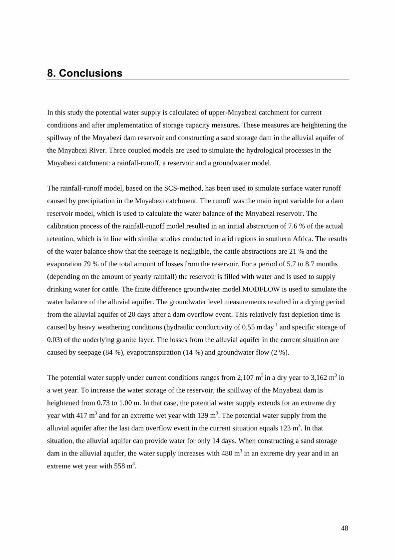
48
8. Conclusions
In this study the potential water supply is calculated of upper-Mnyabezi catchment for current
conditions and after implementation of storage capacity measures. These measures are heightening the
spillway of the Mnyabezi dam reservoir and constructing a sand storage dam in the alluvial aquifer of
the Mnyabezi River. Three coupled models are used to simulate the hydrological processes in the
Mnyabezi catchment: a rainfall-runoff, a reservoir and a groundwater model.
The rainfall-runoff model, based on the SCS-method, has been used to simulate surface water runoff
caused by precipitation in the Mnyabezi catchment. The runoff was the main input variable for a dam
reservoir model, which is used to calculate the water balance of the Mnyabezi reservoir. The
calibration process of the rainfall-runoff model resulted in an initial abstraction of 7.6 % of the actual
retention, which is in line with similar studies conducted in arid regions in southern Africa. The results
of the water balance show that the seepage is negligible, the cattle abstractions are 21 % and the
evaporation 79 % of the total amount of losses from the reservoir. For a period of 5.7 to 8.7 months
(depending on the amount of yearly rainfall) the reservoir is filled with water and is used to supply
drinking water for cattle. The finite difference groundwater model MODFLOW is used to simulate the
water balance of the alluvial aquifer. The groundwater level measurements resulted in a drying period
from the alluvial aquifer of 20 days after a dam overflow event. This relatively fast depletion time is
caused by heavy weathering conditions (hydraulic conductivity of 0.55 m.day-1 and specific storage of
0.03) of the underlying granite layer. The losses from the alluvial aquifer in the current situation are
caused by seepage (84 %), evapotranspiration (14 %) and groundwater flow (2 %).
The potential water supply under current conditions ranges from 2,107 m3 in a dry year to 3,162 m3 in
a wet year. To increase the water storage of the reservoir, the spillway of the Mnyabezi dam is
heightened from 0.73 to 1.00 m. In that case, the potential water supply extends for an extreme dry
year with 417 m3 and for an extreme wet year with 139 m3. The potential water supply from the
alluvial aquifer after the last dam overflow event in the current situation equals 123 m3. In that
situation, the alluvial aquifer can provide water for only 14 days. When constructing a sand storage
dam in the alluvial aquifer, the water supply increases with 480 m3 in an extreme dry year and in an
extreme wet year with 558 m3.

49
The sand storage dams stores water underground, which reduces the evaporation loss from 79 % to
38 % compared to the reservoir. Since the Mnyabezi reservoir dries out after 5.7 to 8.7 months, the
sand storage dam could be used as an additional water resource. The results show that the period of
water supply could be extended for 1.5 to 1.7 months after the reservoir has been dried out. This
makes the total period of water supply 7.2 months in an extreme dry year and 10.4 months in an
extreme wet year. Heightening the spillway will increase this period to respectively 8.4 (total amount
of water supply is 2,776 m3) and 10.8 months (total amount of water supply is 3,617 m3).
The rainfall-runoff model is calibrated on only one rainfall event, which causes a large uncertainty in
the inflow of the reservoir model. Nevertheless, the drying periods of the reservoirs are monitored
quite well. Since the main interest of the study is to calculate the potential water supply after the main
rainy season, the water balance results of the reservoir still provide useable outcomes. Besides, rainfall
events in the arid region of southern Zimbabwe are usually very heavy, which cause dam overflow in
the reservoir and complete saturation of alluvial aquifer anyway. Since the results concerning the sand
storage dam are not validated at this moment the results are uncertain. It would be very interesting to
monitor the hydrological processes of a sand storage dam in situ to reduce this uncertainty. The
suggested implementation of an impermeable bottom-layer to prevent water percolating to the
underlying granite is a new concept, for which the practical implementation needs further research.
This study has researched the hydrological processes in the alluvial aquifer of the Mnyabezi River. For
the Mnyabezi catchment the alluvial aquifer is too small to sustain a large storage capacity, and can
only be used as an additional water resource. However, when an ephemeral river is underlain by a
larger alluvial aquifer, a sand storage dam is a promising way of water supply for smallholder farmers
in southern Zimbabwe. In this study, the main concepts are established for a small catchment.
Possibly, these results can also be used for a better understanding of the hydrological processes in
larger alluvial aquifer systems in the Mzingwane catchment.

50
References
Anderson, N.J. (1997). Modelling the Sustainable Yield of Groundwater Resource in Riverbed Aquifers in Arid and Semi-arid
Areas. MPhil to PhD Transfer Report. London, England: University of London, Department of Civil Engineering.
Arnold, J.G., Allen, P.M. , Bernhardt, G. (1993). A comprehensive surface-ground water flow model. Journal of
Hydrology, 142: 47-69.
Arnold, J.G., Srinivasan, R., Muttiah, R.S., Williams, J.R. (1998). Large area hydrologic modelling and assessment. Part I.
Model development. Journal of the American Water Resource Association, 34: 73–89.
Arnold, J.G., Fohrer, N. (2005). SWAT2000: current capabilities and research opportunities in applied watershed modelling.
Hydrological Processes, 19: 563-572.
Asselt van, B.A., Rotmans, J. (2002). Uncertainty and integrated assessment modelling: From positivism to pluralism.
Climate change, 54: 75-105.
Astatke, A., Bunning, S., Anderson, F. (1986). Building ponds with animal power in the Ethiopian highlands: A manual.
Addis Ababa, Ethiopia: International Livestock Centre for Africa.
Barker, R., Molle, F. (2004). Evolution of irrigation in South and Southeast Asia. Comprehensive Assessment Research
Report 4. Colombo, Ski Lanka: IWMI.
Barnes, C.J., Jacobsson, G, Smith, G.D. (1994). The diffuse recharge mechanism in the Australian arid zone. SSSA Journal,
58: 31 - 40.
Borst, L., DeHaas, S.A. (2006). Hydrology of Sand Storage Dams. A case study in the kiindu catchment, Kitui District,
Kenia. MSc-thesis. Amsterdam, The Netherlands: Vrije Universiteit.
Coates Palgrave, K. (1997). Trees of Southern Africa. Cape Town, South Africa: Struik Publishers.
Davis, S.N. (1969). Porosity and permeabiliy of natural materials. Flow through porous media, ed. R.J.M. De Wiest,
Academic Press, New York, 54-89.
Davis, J., Herbert, R., Rastall, P. (1995). Collector Well Systems for Sand Rivers. Technical Report WD/95/53C. London,
England: British Geological Survey.
Department of Meteorological Services Zimbabwe (1981). Climate Handbook of Zimbabwe. Salisbury (Harare), Zimbabwe:
Department of meteorological Services.
Dingman, S.L. (2002). Physical Hydrology (2nd ed). Upper Sattle River, New Jersey, USA: Prentice-Hall, Inc.
Domenico, P.A., Schwartz, F.W. (1998). Physical and Chemical Hydrogeology (2nd ed.). New York, USA: John Wiley &
Sons, Inc.
El-Kadi, A.I. (1989). Watershed models and their applicability to conjunctive use management. Water Resources Bulletin,
25: 125–137.
Falkenmark, M., Rockström, J. (2003). Balancing Water for Man and Nature: The new approach in Ecohydrology. London,
England: EarthScan.
FAO (1991). Water Harvesting: A manual for the Design and Construction of Water Harvesting Schemes for Plant
Production. AGL/MISC/17/91. Italy, Rome: FAO.
FAO (2004). The State of Food Insecurity in the World: Monitoring progress towards the World Food Summit and
Millennium Development Goals. Italy, Rome: FAO.
Fetter, C.W. (1994). Applied hydrogeology (3rd ed). New York, USA: MacMillian College Publishing Company.
FewsNet (2006). Special Report: El Nino and Indian Ocean Dipole conditions likely into early 2007, with drought and
flooding implications for Southern and Eastern Africa. FewsNet: www.fews.net

51
Gorgens, A.H.M., Boroto, R.A. (1997). Limpopo River: flow balance anomalies, surprises and implications for integrated
water resources management. Pretoria, South Africa: Proceedings of the 8th National Hydrology Symposium.
Gorgens, A.H.M., Lee, J. (1992). Hydrological impacts of forestry; a research planning study. Petoria, South Africa: Water
Resource Commission.
Graf, W.L. (1988). Fluvial processes in dryland rivers. Berlin-Heidelberg, Germany: Springer-Verlag
Hanson, G. (1987). Groundwater dam research and development in the Hararghe Region, Addis Abeda, Ethiopia: National
Water Resource Commission.
Harbaugh, A.W. (2005). A16: MODFLOW-2005, the U.S. Geological Survey modular ground-water module – the Ground-
water flow process. Techniques of Water-Resources Investigations of the United States Geological Survey Book 6,
Modeling Techniques, Section A: Ground Water. Washington, DC: US Geological Survey.
Hazen, A. (1911). Dams on sand foundations. American Society of Civil Engineers, 73: 199-204.
Healy, R.W., Cook, P.G. (2002). Using groundwater levels to estimate recharge, Hydrogeology Journal, 10: 91-109.
Heyns, P., Montgomery, S., Pallett, S., Seely, M.K. (1997). Namibia’s water: A decision makers’ guide. Namibia, Windhoek:
Ministry of Agriculture, Water and Rural Development/Desert Research Foundation of Namibia.
Hill, M.C. (1998). Methods and guideline or effective model calibration. Report 98–4005. Washington, DC: US Geological
Survey Water Resource Investigations.
Hranova, R. (2006). Diffuse pollution of water resources. Principles and case studies in the southern African region. Leiden,
The Netherlands: Taylor & Francis Group/A.A. Balkema Publishers.
Hughes, D.A. (1995). Monthly rainfall–runoff models applied to arid and semi-arid catchments for water resource estimation
purposes. Hydrological Science Journal, 40: 751-769.
Hughes, D.A. (2005). Hydrological issue associated with the determination of environmental water requirements for
ephemeral rivers. River Research and Applications, 21: 899-908.
Hussey, S.W. (2003). The feasibility of sand-abstraction as a viable method of groundwater abstraction. MSc-thesis.
Leicestershire, UK: Loughborough University.
INGC, UEM-Department of Geography and FEWS NET MIND (2003). Atlas for Disaster Preparedness and Response in the
Limpopo Basin. Cape Town, South Africa: Creda Communications (Pty) Ltd.
Jacobson, P.J.; Jacobson, K.M., Seely, M.K. (1995). Ephemeral rivers and their catchments: sustaining people and
development in western Namibia. Windhoek, Namibia: Desert Research Foundation.
Jaspers, F.G.W. (2003). Institutional arrangements for integrated river basin management. Water Policy, 5: 77-90.
Love, D., Jonker, L., Rockström J., van der Zaag, P., Twomlow, S. (2004). The Challenge of Integrated Water Resource
Management for Improved Rural Livelihoods in the Limpopo Basin – an introduction to WaterNet’s first network
research program. In: Abstract volume of the 5th WaterNet-WARFSA Symposium, Windhoek, Namibia.
Love, D., Twomlow, S., Mupangwa, W., van der Zaag, P., Gumbo, B. (2006). Implementing the millennium development
food security goals – challenges of the southern African context. Physics and Chemistry on the Earth, 31: 731-737.
Love, D. (2006a). Land/water/livelihood strategies and water resource availability. 5th Draft PhD Proposal (unpublished).
Harare, Zimbabwe: WaterNet, Challenge Program Project Partnership.
Love, D. (2006b). Alluvial aquifers in the Mzingwane catchment: A preliminary report (Unpublished). Delft, The
Netherlands: UNESCO-IHE.
Love, D. (2006c). Schematization of the Thuli basin. Delft, The Netherlands: UNESCO-IHE.
Maidment, D.R. (1992). Handbook of Hydrology, Texas: R.R. Donnelly & Sons Company.
Maisiri, N., Rockstrom, J., Senzanje, A., Twomlow, S.J. (2005). An on farm evaluation of the effects of low cost drip
irrigation on water and crop productivity, compared to conventional surface irrigation system. Physics and
Chemistry of the Earth, 30: 783–791.
McDonald, M.G. , Harbaugh, A.W. (1988). A modular three-dimensional finite-difference ground-water flow.
Washington, DC: US Geological Survey.

52
Morris, D.A., A.I. Johnson, A.I. (1967). Summary of hydrologic and physical properties of rock and soil materials, as
analysed by the Hydrologic Laboratories of the U.S. Geological Survey 1948-1960. Water Supply Paper, 1839-D.
Washington, DC: U.S. Geological Survey.
Mostert, E., Beek van, E., Bouwman, E., Hey, E., Savenije, H.H.G., Thissen, W.A.H. (1999). River Basin Management and
Planning. Keynote paper for international workshop on River Basin Management, 2nd World Water Forum, The
Hague, 27-19 October 2000.
Moyce, W., Mangeya, P., Owen, R., Love, D. (2006). Alluvial aquifers in the Mzingwane Catchment: their distribution,
properties, current usage and potential expansion. Physics and Chemistry of the Earth, 31: 988-994.
Moyo, M (2001). Representative soil profiles of ICRISAT research sites. Soil report No. A666. Reference No.
1787/FS/5/1/57. Zimbabwe, Harare: Chemistry and Soil Research Institute
Moyo, R., Love, D., Mul, M., Twomlow, S., Mupangwa, W. (2006). Impact and sustainability of drip irrigation kits in the
semi-arid Lower Mzingwane Subcatchment, Limpopo Basin. Physics and Chemistry of the Earth, 31: 885-892
Mudzingwa, B. (1998). Hardrock hydrogeology of the Nyatisme Catchment, Zimbabwe. MSc-thesis. Enschede, The
Netherlands,: ITC.
Mwakalila, S. (2006). Socio-economic impacts of irrigated agriculture in Mbarali District of South-West Tanzania. Physics
and Chemistry of the Earth, 31: 876-884
Mwenge Kahinda, J.M. (2004). Water productivity and yield cap analysis of water harvesting systems in the semi arid
Mzingwane catchment, Zimbabwe. MSc-thesis. Harare: University of Zimbabwe, Department of Civil Engineering.
Nash, J.E., Sutcliffe, J.V. (1970). River flow forecasting through conceptual models. Part I – A discussion of principles.
Journal of hydrology, 10: 282–290.
Neretnieks, I., Abelin, H., Birgersson, L., Moreno, L., Widen, H., Argen, T. (1990). A large scale flow and tracer experiment
in granite, in Hydrology of Low Permeability Environments, S.P. Neuman and I Neretnieks (Eds.), International
Association of Hydrologists.
Nord, M. (1985). Sand Rivers of Botswana, Results from phase 2 of the Sand Rivers Project. Gaborone: Government of
Botswana, Department of Water Affairs.
Osman, Y.Z., Bruen, M.P. (2002). Modelling stream- aquifer seepage in an alluvial aquifer; an improved loosing-stream
package for MODFLOW, Journal of Hydrology, 264: 69-86.
Owen R.J. (1991). Water resources for small scale irrigation from shallow alluvial aquifers in the communal lands of
Zimbabwe. MPhil-thesis. Harare: University of Zimbabwe, Department of Civil Engineering.
Owen, R.J, Dahlin, T. (2005). Alluvial aquifers at geological boundaries: geophysical investigations and groundwater
resources. Groundwater and Human Development, pp233-246. Rotterdam: AA Balkema Publishers.
Rossouw, L., Avenant, M.F., Seaman, M.T., King, J.M., Barker, C.H., Du Preez, P.J., Pelser, A.J., Roos, J.C., Staden van
J.J., Tonder van, G.J., Watson, M. (2005). Environmental water requirements in non-perennial rivers. South
Africa, Bloemfontijn: University of Free State, The Centre of Environmental Science.
Rushton, K.R.; Weller, J. (1985). Response to pumping of a weathered granite aquifer, Journal of Hydrology, 80: 299-309.
Sanchez, P.A., Swaminathan, M.S. (2005). Hunger in Africa: the link between unhealthy people and unhealthy soils. Lancet,
365: 442–444.
Sandstrom, K. (1997). Ephemeral rivers in the tropics. Hydrological processes and water resources assessment and
management: a review and pathfinder. Research Report No. 8. EPOS. Linkoping, Sweden: Linkoping University,
Institute of Tema Research.
Schicht R.J., Walton W.C. (1961). Hydrologic budgets for three small watersheds in Illinois. Illinois, US: State Water Surv
Rep Invest 40.
Schulze, R.E.; Schmidt, E.J.; Smithers, J.C. (1993). SCS-SA User Manual: PC-Based SCS design flood estimates for small
catchments in Southern Africa. In ACRU Report No 40, University of Natal, South Africa.

53
Seely, M., Henderson, J., Heyns, P., Jacobson, P., Nakale, T., Nantanga, K., Schachtschneider, K., 2003. Ephemeral and
endorheic river systems: Relevance and management challenges. In: Turton, A., Ashton, P. and Cloete, E. (eds).
Transboundary rivers, sovereignty and development: Hydropolitical drivers in the Okavango River basin. Pretoria,
South Africa.
Shaw, E.M. (1994). Hydrology in Practice (3rd Ed.). Abington, England: Routledge.
Shephard, R.G. (1989). Geology and ground water in Door Country, Wisconsin, with emphasis on contamination potential in
the Silurian dolomite. Washinton, DC: US Geological Survey Water-Supply Paper 2047.
Sophocleous, M., Perkins, S.P. (2000). Methodology of application of combined watershed and ground-water models in
Kansas, Journal of hydrology, 236: 185-201.
Thiessen, A.H. (1911). Precipitation for large areas. Mon. Wealth. Review, 39: 1082-1084.
Todd, D.K. (1980). Groundwater Hydrology (2nd Ed). New York: John Wiley & Sons Inc.
Townley, L.R. (1998). Shallow groundwater systems. International Contributions to Hydrogeology 18, pp3-12. Rotterdam:
AA Balkema Publishers.
Turnbull, M. (2002). Life in the extreme. Africa Geographic, June 2003: 46-51.
Twomlow, S., Riches, C., O’Neill, D., Brookes, P., Ellis-Jones, J. (1999). Sustainable dryland smallholder farming in
Sub-Saharan Africa. Annals of Arid Zone, 38: 93-135.
Twomlow, S., Bruneau, P. (2000). Semi-arid soil water regimes in Zimbabwe. Geoderma, 95: 33-51.
Uhlenbrook, S., Roser, S., Tilch, N. (2004). Hydrological process representation at the meso-scale: the potential of a
distributed, conceptual catchment model. Journal of Hydrology, 291: 278-296.
UN Millennium Project. (2005). Investing in Development: A Practical Plan to Achieve the Millennium Development Goals.
New York: UNDP.
USDA-Soil Conservation Service (1972). National engineering handbook, Section 4, Hydrology. Washington, DC: USDA-
Soil Conservation Service.
USDA-Soil Conservation Service (1986). Technical Release 55: urban hydrology for small watersheds. Washington, DC:
USDA-Soil Conservation Service.
Vries, de J.J., Simmers, I. (2002). Groundwater recharge: an overview of processes and challenges. Hydrogeology Journal,
10: 5-17.
Walker, W.E., Harremoes, P, Rotmans, J., Van der Sluis, J.P., Van Asselt, M.B.A., Janssen, P., Krayer von Krauss, M.P.
(2003). Defining Uncertainty: A conceptual basis for uncertainty management in model-based decision support.
Integrated Assessment, 4: 5-17.
Waterloo Hydrologic (2006). Helpfile Visual MODFLOW vs 4.2. Canada, Waterloo Hydrologic Inc.
WaterNet (2001). Constitution of WaterNet. Harare, Zimbabwe: WaterNet.
WaterNet (2004). Integrated Water Resource Management for Improved Rural Livelihoods: managing risks, mitigate
drought and improving water productivity in the water scares Limpopo basin. Harare, Zimbabwe: WaterNet,
Challenge Program Project Partnership.
Weglarczyk, S. (1998). The interdependence and applicability of some statistical quality measures for hydrological models.
Journal of Hydrology, 206: 98–103.
Wikner, T. (1980). Sand Rivers of Botswana. Results from phase 1 of the Sand Rivers Project. Gaborone: Government of
Botswana, Department of Water Affairs.
Wipplinger, O. (1958). Storage of Water in Sand. Namibia, Windhoek: South West Africa Administration Water Affair
Branch.
Woltering, L. (2005). Estimating the influence of on-farm Conservation Practices on the Water Balance: Case of the
Mzinyathini Catchment in Zimbabwe. MSc-thesis (unpublished), Delft, The Netherlands: Technical University
Delft, Department of Civil Engineering.

54
Appendices
Appendix I: Grid MODFLOW model................................................................................................... 55 Appendix II: Satellite image study area ................................................................................................ 56 Appendix III: Thiessen polygons Mnyabezi catchment ........................................................................ 57 Appendix IV: Thiessen polygons Bengu catchment ............................................................................. 58 Appendix V: Tables for CN-values....................................................................................................... 59 Appendix VI: Tables for hydro-geological characteristics.................................................................... 60 Appendix VII: Rainfall data .................................................................................................................. 61 Appendix VIII: Open water evaporation data ....................................................................................... 63 Appendix IX: Water level reservoir data............................................................................................... 65 Appendix X: Abstractions Mnyabezi reservoir ..................................................................................... 67 Appendix XI: Abstractions Bengu reservoir ......................................................................................... 68 Appendix XII: Abstractions people....................................................................................................... 71 Appendix XIII: Sieving tests soil .......................................................................................................... 73 Appendix XIV: Sieving tests alluvial material...................................................................................... 75 Appendix XV: Dimension Mnyabezi reservoir..................................................................................... 78 Appendix XVI: Dimension Bengu reservoir......................................................................................... 79 Appendix XVII: Dimensions of the alluvial aquifer ............................................................................. 80 Appendix XVIII: Groundwater table data alluvial aquifer.................................................................... 84 Appendix IXX: Results dam overflow.................................................................................................. 87 Appendix XX: Qualitative uncertainty analyses ................................................................................... 88
55
Appendix I: Grid MODFLOW model
Figure I.1: Cross-section; green = alluvial, bleu = soil, white = granite
Figure I.2: Cross-section representing the water level after 20 days
Figure I.3: Top-view water level after 20 days

56
Appendix II: Satellite image study area
Figure II.1: Satellite image (band 3,4,5 false colour composite of Landsat Scene p170r075, dated 02-06-2000)
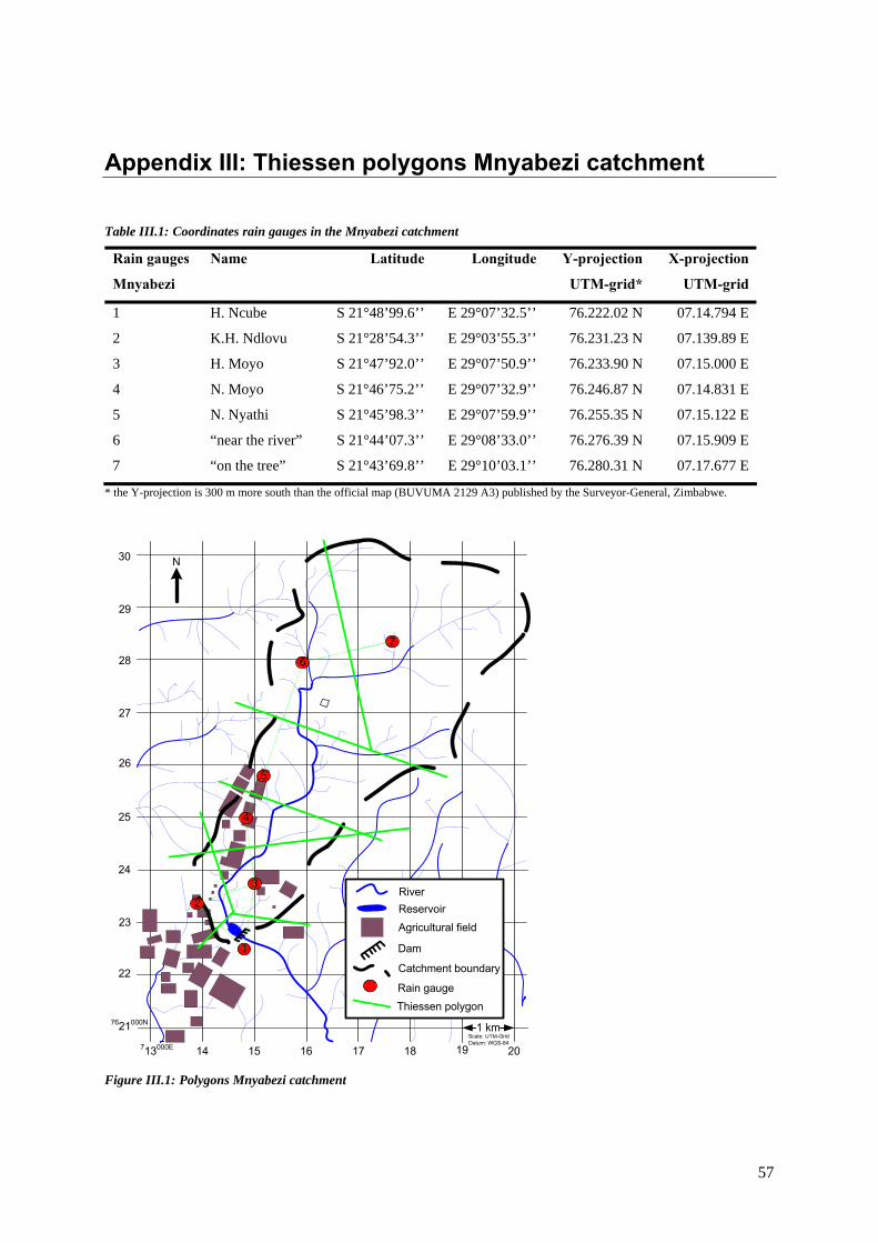
57
Appendix III: Thiessen polygons Mnyabezi catchment Table III.1: Coordinates rain gauges in the Mnyabezi catchment
Rain gauges
Mnyabezi
Name Latitude Longitude Y-projection
UTM-grid*
X-projection
UTM-grid
1 H. Ncube S 21°48’99.6’’ E 29°07’32.5’’ 76.222.02 N 07.14.794 E
2 K.H. Ndlovu S 21°28’54.3’’ E 29°03’55.3’’ 76.231.23 N 07.139.89 E
3 H. Moyo S 21°47’92.0’’ E 29°07’50.9’’ 76.233.90 N 07.15.000 E
4 N. Moyo S 21°46’75.2’’ E 29°07’32.9’’ 76.246.87 N 07.14.831 E
5 N. Nyathi S 21°45’98.3’’ E 29°07’59.9’’ 76.255.35 N 07.15.122 E
6 “near the river” S 21°44’07.3’’ E 29°08’33.0’’ 76.276.39 N 07.15.909 E
7 “on the tree” S 21°43’69.8’’ E 29°10’03.1’’ 76.280.31 N 07.17.677 E
* the Y-projection is 300 m more south than the official map (BUVUMA 2129 A3) published by the Surveyor-General, Zimbabwe.
713000E 14 15 16 17 18 19 20
7621000N
24
25
26
27
28
29
30
23
22
River
Agricultural field
Catchment boundary
Reservoir
Dam
N
5
7
6
3
4
1
2
Rain gaugeThiessen polygon
Scale: UTM-GridDatum: WGS-84
1 km
Figure III.1: Polygons Mnyabezi catchment

58
Appendix IV: Thiessen polygons Bengu catchment Table IV.1: Coordinates rain gauges in the Bengu catchment
Rain gauges
Bengu
Name Latitude Longitude Y-projection
UTM-grid*
X-projection
UTM-grid
1 Bengu School S 21°30’39.0’’ E 29°03’01.8’’ 76.199.21 N 07.124.07 E
2 K. Ngwenya S 21°30’19.3’’ E 29°03’40.5’’ 76.205.12 N 07.135.28 E
3 N. Denya S 21°29’48.4’’ E 29°03’31.4’’ 76.214.65 N 07.132.79 E
4 K.F. Ndlovu S 21°29’48.8’’ E 29°03’41.4’’ 76.214.49 N 07.135.67 E
5 T. Moyo S 21°29’35.2’’ E 29°03’29.9’’ 76.218.74 N 07.132.42 E
6 F. Nyathi S 21°29’35.4’’ E 29°03’44.0’’ 76.218.63 N 07.136.47 E
7 K.H. Ndlovu S 21°28’54.3’’ E 29°03’55.3’’ 76.231.23 N 07.139.89 E
* the Y-projection is 300 m more south than the official map (BUVUMA 2129 A3) published by the Surveyor-General, Zimbabwe.
Table IV.2: CN-values of Thiessen-polygons in the Bengu catchment
711000E 12 13 14 15 16 17 18
7619000N
22
23
24
21
20
River
Agricultural field
Catchment boundary
Reservoir
Dam
N
Rain gaugeThiessen polygon
Scale: UTM-GridDatum: WGS-84
1 km
1
2
3 4
5 6
7
Main road
Figure IV.1: Polygons Bengu catchment
Polygon Area [ha] Rangeland
[%]
Fields [%] Farmsteads
[%]
Hydological
condition
CN-value [-]
1 50 90 0 10 (5 farms) Poor 67.1
2 130 76 20 4 (5 farms) Poor 68.4
3 80 63 31 6 (5 farms) Poor 68.7
4 100 48 50 2 (2 farms) Poor 69.8
5 100 36 60 4 (4 farms) Fair 63.2
6 90 37 60 3 (3 farms) Fair 63.1
7 150 85 13 2 (3 farms) Fair 52.2

59
Appendix V: Tables for CN-values
Table V.1: Curve numbers for hydrological soil cover complexes for AMC class II (SCS, 1972)
Table VI.2: Seasonal rainfall limits to determine AMC classes (SCS, 1972)
Table V.3: Conversion table from AMC class II to AMC class I and III (SCS, 1972)
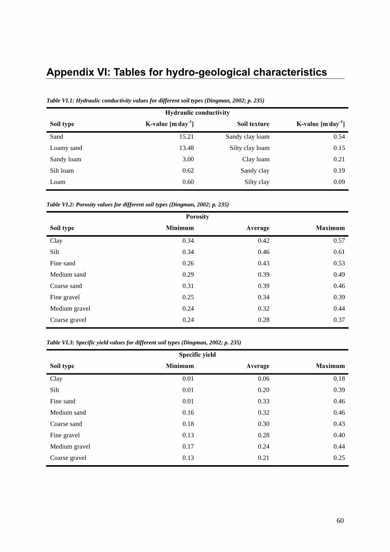
60
Appendix VI: Tables for hydro-geological characteristics
Table VI.1: Hydraulic conductivity values for different soil types (Dingman, 2002; p. 235)
Hydraulic conductivity
Soil type K-value [m.day-1] Soil texture K-value [m.day-1]
Sand 15.21 Sandy clay loam 0.54
Loamy sand 13.48 Silty clay loam 0.15
Sandy loam 3.00 Clay loam 0.21
Silt loam 0.62 Sandy clay 0.19
Loam 0.60 Silty clay 0.09
Table VI.2: Porosity values for different soil types (Dingman, 2002; p. 235)
Porosity
Soil type Minimum Average Maximum
Clay 0.34 0.42 0.57
Silt 0.34 0.46 0.61
Fine sand 0.26 0.43 0.53
Medium sand 0.29 0.39 0.49
Coarse sand 0.31 0.39 0.46
Fine gravel 0.25 0.34 0.39
Medium gravel 0.24 0.32 0.44
Coarse gravel 0.24 0.28 0.37
Table VI.3: Specific yield values for different soil types (Dingman, 2002; p. 235)
Specific yield
Soil type Minimum Average Maximum
Clay 0.01 0.06 0.18
Silt 0.01 0.20 0.39
Fine sand 0.01 0.33 0.46
Medium sand 0.16 0.32 0.46
Coarse sand 0.18 0.30 0.43
Fine gravel 0.13 0.28 0.40
Medium gravel 0.17 0.24 0.44
Coarse gravel 0.13 0.21 0.25

61
Appendix VII: Rainfall data Mnyabezi
Table VII.1: Rainfall data Mnyabezi catchment (*estimate)
Rain gauge number
Date 1 [mm] 2 [mm] 3 [mm] 4 [mm] 5 [mm] 6 [mm] 7 [mm]
11-03-2007 0 0 0 0 0 0 0
…
27-03-2007 0 0 0 0 0 0 0
28-03-2007 1 3 2 0 0 0 1
29-03-2007 40 39.5 40 48 50 60 70
30-03-2007 10 4 5 10 10 20 20*
31-03-2007 0 5 0 0 0 0 0
01-04-2007 0 0 0 0 0 0 0
02-04-2007 0 0 0 0 0 0 0
03-04-2007 0 4 0 0 0 0 0
04-04-2007 0 3 0 0 0 0 0
05-04-2007 21 15 23 5 20 30 2.5
06-04-2007 0 0 0 0 0 0 0
…
03-05-2007 0 0 0 0 0 0 0
Bengu
Table VII.2: Rainfall data Bengu catchment
Rain gauge number
Date 1 [mm] 2 [mm] 3 [mm] 4 [mm] 5 [mm] 6 [mm] 7 [mm]
10-02-2007 9 8 5 4 2 2 0
11-02-2007 2 2 1.5 1.5 1.5 1 0
12-02-2007 0 0 0 0 0 0 0
13-02-2007 0 0 0 0 0 0 0
14-02-2007 0 0 0 0 0 0 0
15-02-2007 0 0 0 0 0 0 0
16-02-2007 0 0 0 0 0 0 0
17-02-2007 0 0 0 0 0 0 0
18-02-2007 0 0 0 0 0 0 0
19-02-2007 5 4.5 7 8 8 8 16
20-02-2007 0 0 0 0 0 0 0

62
Rain gauge number
Date 1 [mm] 2 [mm] 3 [mm] 4 [mm] 5 [mm] 6 [mm] 7 [mm]
21-02-2007 0 0 0 0 0 0 0
22-02-2007 0 0 0 0 0 0 0
23-02-2007 0 0 0 0 0 0 0
24-02-2007 0 0 0 0 0 0 0
25-02-2007 0 0 0 0 0 0 0
26-02-2007 0 0 0 0 0 0 0
26-02-2007 26 20 30 30 30 32 40
27-02-2007 1.5 1 1.5 1.5 1.5 1.5 2.5
28-02-2007 0 0 0 0 0 0 0
…
27-03-2007 0 0 0 0 0 0 0
28-03-2007 2 2 2 2 2 2 3
29-03-2007 32 36 36 36 32 28 39.5
30-03-2007 12 16 19 20 14 15 4
31-03-2007 2 1 2 2 2 3 5
01-04-2007 0 0 0 0 0 0 0
02-04-2007 0 0 0 0 0 0 0
03-04-2007 3 4 4 6 5 6 4
04-04-2007 1.5 1.5 2 1.5 2 2 3
05-04-2007 1.5 10 12 12 15 16 15
06-04-2007 0 0 0 0 0 0 0
…
03-05-2007 0 0 0 0 0 0 0

63
Appendix VIII: Open water evaporation data Table VIII.1: Open water evaporation data (* rainfall rate ** estimated value before refill pan)
Date Reading evaporation
pan [mm]
Weather
during the day
Pan- evaporation
[mm.day-1]
Evaporation with
Pan factor [mm.day-1]
11-03-2007 46 Clear 10 7.0
12-03-2007 56 Clear 10 7.0
13-03-2007 66 Clear 10 7.0
14-03-2007 76 Clear 10 7.0
15-03-2007 86 Clear 10 7.0
16-03-2007 96 Clear 10 7.0
17-03-2007 106 A few clouds 10 7.0
18-03-2007 116 A few clouds 12 8.4
19-03-2007 128 Totally clouded 2 1.4
20-03-2007 130** - 74 Moderately clouded 9 6.3
21-03-2007 83 Clear 13 9.1
22-03-2007 96 Clear 11 7.7
23-03-2007 107 A few clouds 7 4.9
24-03-2007 114 Clear 12 8.4
25-03-2007 126 Clear 10 7.0
26-03-2007 136 A few clouds 9 6.3
27-03-2007 145** – 74 Heavily cloudy 4 2.8
28-03-2007 76 (2 mm*) Totally clouded 3 2.1
29-03-2007 47 (32 mm*) Totally clouded 7 4.9
30-03-2007 42 (12 mm*) Totally clouded 2 1.4
31-03-2007 42 (2 mm*) Totally clouded 2 1.2
01-04-2007 44 Totally clouded 4 2.8
02-04-2007 48 Heavily clouded 3 2.1
03-04-2007 48 (3 mm*) Totally clouded 3.5 2.5
04-04-2007 50 (1.5 mm*) Totally clouded 5.5 3.9
05-04-2007 53 (1.5 mm*) Totally clouded 5 3.5
06-04-2007 58 Totally clouded 5 3.5
07-04-2007 63 Totally clouded 6 4.2
08-04-2007 69 Totally clouded 3 2.1
09-04-2007 72 Totally clouded 4 2.8
10-04-2007 76 Moderate clouded 6 4.2
11-04-2007 82 Clear 10 7.0

64
Date Reading evaporation
pan [mm]
Weather during the
day
Pan-evaporation
[mm.day-1]
Evaporation with
pan factor [mm.day-1]
12-04-2007 92 Moderate clouded 6 4.2
13-04-2007 98 Heavily clouded 4 2.8
14-04-2007 102 A few clouds 5 3.5
15-04-2007 107 Clear 9 6.3
16-04-2007 116 Clear 6 4.2
17-04-2007 122 Clear 9 6.3
18-04-2007 131 A few clouds 8 5.6
19-04-2007 139 – 64 Moderate clouded 8 5.6
20-04-2007 72 Clear 9 6.3
21-04-2007 81 Clear 11 7.7
22-04-2007 92 Clear 7 7.0
23-04-2007 99 A few clouds 6 6.3
24-04-2007 105 Clear 8 5.6
25-04-2007 113 Clear 8 5.6
26-04-2007 121 Clear 14 9.8
27-04-2007 135 – 22 Clear 8 5.6
28-04-2007 30 Heavily clouded 7 4.9
29-04-2007 37 Clear 10 7.0
30-04-2007 47 Clear 8 5.6
01-05-2007 55 Clear 9 7.3
02-05-2007 64 Heavily clouded 6 4.2
03-05-2007 7 A few clouds 8.6*** 6.0***
Average evaporation March: 6.0 mm
Average evaporation April: 5.0 mm
Average evaporation clear sky: 6.9 mm
Average evaporation with a few clouds: 6.0 mm
Average evaporation moderate clouded: 5.1 mm
Average evaporation heavily clouded: 3.4 mm
Average evaporation totally clouded: 2.8 mm

65
Appendix IX: Water level reservoir data
Table IX.1: Water level Mnyabezi and Bengu reservoirs (* estimates)
Date Mnyabezi
reservoir [cm]
Difference [cm] Bengu
reservoir [cm]
Difference [cm]
11-03-2007 57.8 35.1
12-03-2007 57.0 - 0.8 34.2 - 0.9
13-03-2007 56.3 - 0.7 33.1 - 1.1
14-03-2007 54.0 - 2.3 32.0* - 1.1
15-03-2007 52.2 - 1.8 31.1 - 1.1
16-03-2007 50.0 - 2.2 30.8 - 0.3
17-03-2007 48.3 -1.7 29.8 - 1.0
18-03-2007 47.5 - 0.8 28.1 - 1.7
19-03-2007 47.1 - 0.4 27.8 - 0.3
20-03-2007 46.5 - 0.6 27.0 - 0.8
21-03-2007 45.3 - 0.8 26.2 - 0.8
22-03-2007 45.1* - 0.2 25.3 - 0.9
23-03-2007 44.9* - 0.2 24.1 - 1.2
24-03-2007 44.0 - 0.9 23.3* - 0.8
25-03-2007 43.0* - 1.0 21.8* - 1.5
26-03-2007 42.0 - 1.0 20.2 - 1.6
27-03-2007 41.5 - 0.5 18.8 - 1.4
28-03-2007 40.0 -1.5 17.5 - 1.3
29-03-2007 76.0 + 36.0 73.2 + 65.8
30-03-2007 78.0 + 2.0 80.0 + 6.8
31-03-2007 75.0 - 3.0 72.0 - 8.0
01-04-2007 72.1* - 2.9 68.2 - 3.8
02-04-2007 71.0 - 1.1 66.0 - 2.2
03-04-2007 70.0 - 1.0 65.8 - 0.2
04-04-2007 69.0 - 1.0 64.8 - 1.0
05-04-2007 73.0* + 4.0 63.7 - 1.1
06-04-2007 72.0* - 1.0 62.2* - 1.5
07-04-2007 71.0* -1.0 60.7* - 1.5
08-04-2007 70.0* -1.0 59.2* - 1.5
09-04-2007 69.0 -1.0 58.0 - 1.2
10-04-2007 68.0 -1.0 58.8 - 0.8
11-04-2007 67.0 - 1.0 57.9 - 0.9
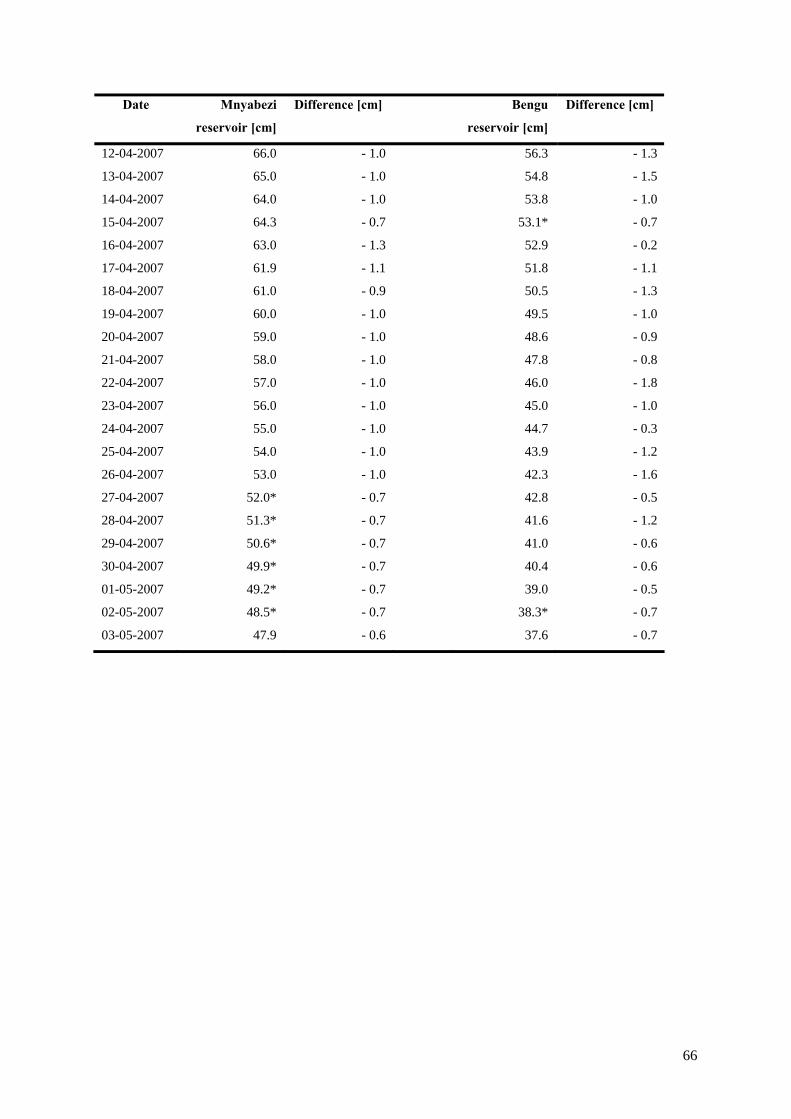
66
Date Mnyabezi
reservoir [cm]
Difference [cm] Bengu
reservoir [cm]
Difference [cm]
12-04-2007 66.0 - 1.0 56.3 - 1.3
13-04-2007 65.0 - 1.0 54.8 - 1.5
14-04-2007 64.0 - 1.0 53.8 - 1.0
15-04-2007 64.3 - 0.7 53.1* - 0.7
16-04-2007 63.0 - 1.3 52.9 - 0.2
17-04-2007 61.9 - 1.1 51.8 - 1.1
18-04-2007 61.0 - 0.9 50.5 - 1.3
19-04-2007 60.0 - 1.0 49.5 - 1.0
20-04-2007 59.0 - 1.0 48.6 - 0.9
21-04-2007 58.0 - 1.0 47.8 - 0.8
22-04-2007 57.0 - 1.0 46.0 - 1.8
23-04-2007 56.0 - 1.0 45.0 - 1.0
24-04-2007 55.0 - 1.0 44.7 - 0.3
25-04-2007 54.0 - 1.0 43.9 - 1.2
26-04-2007 53.0 - 1.0 42.3 - 1.6
27-04-2007 52.0* - 0.7 42.8 - 0.5
28-04-2007 51.3* - 0.7 41.6 - 1.2
29-04-2007 50.6* - 0.7 41.0 - 0.6
30-04-2007 49.9* - 0.7 40.4 - 0.6
01-05-2007 49.2* - 0.7 39.0 - 0.5
02-05-2007 48.5* - 0.7 38.3* - 0.7
03-05-2007 47.9 - 0.6 37.6 - 0.7

67
Appendix X: Abstractions Mnyabezi reservoir Table X.1: Abstractions by cattle from the Mnyabezi reservoir
Name Cows
[-]
Calves
[-]
Goats
[-]
Kids
[-]
Donkeys
[-]
Water use livestock
[l.day-1] *
1 D. Dube 8 3 12 1 9 472
2 T. Madzikiti 11 2 11 4 3 418
3 M. Mdlongwa 10 3 6 5 4 400
4 H. Moyo 8 2 10 5 9 460
5 Ja. Moyo 4 1 14 2 5 284
6 Jo. Moyo 2 0 30 0 11 420
7 K. Moyo 4 1 15 1 4 267
8 M. Moyo 3 1 7 4 9 308
9 N. Moyo 7 1 9 1 2 272
10 Sa. Moyo 3 0 5 0 5 200
11 Sh. Moyo 2 1 9 0 2 145
12 O. Nare 30 3 20 1 10 1,082
13 T. Nare 1 1 29 30 9 420
14 H. Ncube 5 1 13 5 4 290
15 W. Ncube 3 1 4 2 0 109
16 J. Ndlovu 9 3 15 0 5 430
17 M. Ndlovu 34 10 32 10 12 1,370
18 G. Ndlovu 5 1 12 3 6 321
19 S. Ngulube 5 2 5 0 3 230
20 M. Ngwenya 9 2 15 3 6 446
21 O. Ngwenya 10 3 20 4 6 508
22 El. Nyathi 8 1 32 15 4 480
23 Ep. Nyathi 16 6 20 10 6 700
24 F. Nyathi 2 2 24 0 5 290
25 K. Nyathi 1 1 8 7 4 169
26 N. Nyathi 4 3 4 2 4 234
27. P. Nyathi 20 6 30 10 7 870
Total 224 61 411 125 153 11,595
* 1 cow uses 25 l.day-1 1 calve uses 10 l.day-1
1 donkey uses 20 l.day-1 1 kid uses 2 l.day-1
1 goat uses 5 l.day-1

68
Appendix XI: Abstractions Bengu reservoir Table XI.1: Abstractions by cattle from the Bengu reservoir
Name Cows
[-]
Calves
[-]
Goats
[-]
Kids
[-]
Donkeys
[-]
Water use livestock
[l.day-1] *
1 T. Bedza 0 0 8 3 2 86
2 E. Chinamure 10 3 32 12 4 544
3 N. Denya 0 0 15 6 6 207
4 B. Dube 6 2 25 10 3 375
5 El. Dube 1 0 10 2 6 199
6 Ev. Dube 6 2 10 2 5 324
7 P. Dube 5 2 15 5 2 270
8 A. Homela 0 0 5 2 0 29
9 D. Khumalo 0 0 10 3 0 56
10 C. Mabetha 5 2 8 2 4 269
11 M. Mabetha 1 0 4 4 3 113
12 S. Mabhena 0 0 13 2 0 69
13 E. Malutha 0 0 14 6 7 222
14 T. Malutha 0 0 15 7 0 89
15 H. Magaya 13 0 38 21 0 557
16 K. Magaya 0 0 15 4 5 183
17 G. Maphosa 0 0 6 1 6 152
18 Nd. Maphosa 0 0 8 2 2 84
19 Nk. Maphosa 0 0 8 2 0 44
20 G. Mapfumo 5 2 39 11 7 502
21 V. Masendeke 2 1 2 0 0 70
22 K. Masiane 0 0 12 4 0 68
23 S. Masiane 0 0 15 5 3 145
24 M. Masiane 0 0 10 3 4 136
25 L. Masuku 10 4 28 5 6 560
26 E. Mathe 20 4 35 10 1 755
27 M. Mathe 3 3 3 4 3 188
28 S. Mathnodi 0 0 10 3 3 116
29 N. Mbedzi 0 0 15 5 7 225
30 Al. Moyo 31 10 44 12 4 1,199
31 Au. Moyo 0 0 10 0 0 50
32 A. S. Moyo 5 1 20 5 5 345

69
Name Cows
[-]
Calves
[-]
Goats
[-]
Kids
[-]
Donkeys
[-]
Water use livestock
[l.day-1] *
33 G. Moyo 0 0 10 0 0 50
34 L. Moyo 8 2 28 6 6 492
35 M. Moyo 4 2 29 9 6 403
36 O. Moyo 35 5 46 21 10 1,397
37 P. Moyo 0 0 12 2 3 124
38 S. Moyo 22 10 46 12 9 1,084
39 T. Moyo 12 3 21 6 4 527
40 S. Mpofu 15 3 32 10 6 705
41 S. Mtembo 6 2 21 7 8 449
42 A. Nare 0 0 2 0 0 10
43 B. Nare 0 0 9 1 0 47
44 E. Nare 0 0 28 12 4 244
45 L. Nare 2 1 5 1 6 207
46 Ma. Nare 10 3 22 6 7 542
47 Me. Nare 4 0 10 3 4 236
48 S. Nare 6 2 39 12 8 549
49 Th. Nare 0 0 8 2 0 44
50 Ti. Nare 5 2 12 3 8 371
51 Ts. Nare 0 0 13 4 6 193
52 B. Ncube 28 7 52 12 6 1,174
53 D. Ncube 8 4 35 6 8 587
54 H. Ncube 12 4 38 12 9 734
55 K. Ncube 0 0 38 9 6 328
56 Lu. Ncube 0 0 5 1 0 27
57 Le. Ncube 0 0 9 10 3 125
58 N. Ncube 0 0 7 3 4 121
59 O. Ncube 8 2 15 6 6 427
60 R. Ncube 0 0 15 5 4 165
61 S. Ncube 0 0 21 7 0 119
62 Ma. Ndlovu 6 2 12 3 0 236
63 Mi. Ndlovu 10 3 20 6 6 512
64 E. Ndlovu 0 0 28 8 6 276
65 Joi. Ndlovu 0 0 15 5 5 185
66 Jon. Ndlovu 0 0 12 4 0 68
67 N. Ndlovu 6 2 21 6 6 407
68 Sim. Ndlovu 8 3 24 9 6 488
69 Sip. Ndlovu 1 0 5 2 0 54
70 Sit. Ndlovu 0 0 15 6 6 207

70
Name Cows
[-]
Calves
[-]
Goats
[-]
Kids
[-]
Donkeys
[-]
Water abstraction
[l.day-1] *
71 T. Ndlovu 3 1 0 0 0 85
72 G. Ngulube 0 0 6 3 0 36
73 L. Ngulube 0 0 15 5 0 85
74 K. Ngwenya 6 2 24 9 12 548
75 T. Ngwenya 0 0 10 3 0 56
76 P. Nkala 7 3 0 0 6 325
77 F. Nkomo 0 0 5 1 0 27
78 L. Ntini 0 0 18 6 3 162
79 A. Nyathi 0 0 8 3 4 126
80 B. Nyathi 0 0 10 1 0 52
81 Md. Nyathi 41 12 52 15 12 1,675
82 Mi. Nyathi 28 8 45 15 8 1,195
83 O. Nyathi 58 15 30 10 9 1,950
84 P. Nyathi 0 0 9 3 2 91
85 T. Nyathi 0 0 30 12 16 494
86 M. Nyoni 0 0 10 2 3 114
87 B. Sibanda 0 0 30 10 3 230
88 E. Sibanda 0 0 16 6 0 92
89 H. Sibanda 0 0 4 1 0 22
90 S. Sibanda 0 0 15 4 0 83
91 R. Sebata 31 11 42 18 10 1,331
92 T. Sijiye 0 0 15 4 6 203
93 K. Sithole 0 0 15 8 3 151
94 D. Tlou 0 0 52 15 8 450
95 P. Zhou 0 0 6 1 0 32
Total 513 150 1,749 555 379 31,760
* 1 cow uses 25 l.day-1
1 donkey uses 20 l.day-1
1 goat uses 5 l.day-1
1 calve uses 10 l.day-1
1 kid uses 2 l.day-1

71
Appendix XII: Abstractions people Table XII.1: Pump abstractions for domestic use in the Mnyabezi catchment
Name Water use
11 April
[l.day-1]
Water use
24 April
[l.day-1]
Water use
27 April
[l.day-1]
Water use
28 April
[l.day-1]
Water use
30 April
[l.day-1]
Average
water use
[l.day-1]
1 D. Dube 120 140 120 140 140 132
2 T. Madzikiti 200 200 200 120 120 168
3 M. Mdlongwa 80 100 160 30 60 86
4 H. Moyo 120 160 140 160 160 148
5 Ja. Moyo 40 80 80 210 200 122
6 Jo. Moyo 160 100 160 140 140 140
7 K. Moyo 100 100 100 200 200 140
8 M. Moyo 240 140 240 140 80 168
9 N. Moyo 100 160 120 200 80 132
10 Sa. Moyo 200 200 200 180 180 192
11 Sh. Moyo 80 80 180 160 160 132
12 O. Nare 120 120 120 160 160 136
13 T. Nare 60 120 80 40 80 76
14 H. Ncube 140 120 140 130 120 130
15 W. Ncube 120 100 120 80 80 100
16 J. Ndlovu 100 130 130 140 140 128
17 M. Ndlovu 200 200 200 140 180 184
18 G. Ndlovu 120 80 180 120 180 136
19 S. Ngulube 130 80 80 40 40 74
20 M. Ngwenya 180 200 100 200 70 150
21 O. Ngwenya 100 100 80 210 200 138
22 El. Nyathi 160 140 120 120 40 116
23 Ep. Nyathi 160 180 200 100 120 152
24 F. Nyathi 180 180 130 180 180 170
25 K. Nyathi 80 60 90 60 60 70
26 N. Nyathi 120 120 200 80 80 120
27 P. Nyathi 120 200 200 100 100 144
Total 3,530 3,590 3,870 3,580 3,350 3,584

72
Table XII.2: Pump abstractions for gardening in the Bengu catchment (* gardens are 100 m2)
Name Water use [l.day-1]*
1 N. Denya 380
2 N. Mabetha 540
3 L .Magaya 160
4 A. Masuku 200
5 E. Mathe 400
6 E. Nare 600
7 Sip. Ndolvu 100
8 Sit. Ndlovu 320
9 C. Phiri 460
10 B. Sibanda 460
11 H. Sibanda 200
Average 347
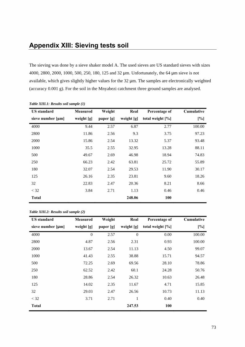
73
Appendix XIII: Sieving tests soil
The sieving was done by a sieve shaker model A. The used sieves are US standard sieves with sizes
4000, 2800, 2000, 1000, 500, 250, 180, 125 and 32 μm. Unfortunately, the 64 μm sieve is not
available, which gives slightly higher values for the 32 μm. The samples are electronically weighted
(accuracy 0.001 g). For the soil in the Mnyabezi catchment three ground samples are analysed.
Table XIII.1: Results soil sample (1)
US standard
sieve number [μm]
Measured
weight [g]
Weight
paper [g]
Real
weight [g]
Percentage of
total weight [%]
Cumulative
[%]
4000 9.44 2.57 6.87 2.77 100.00
2800 11.86 2.56 9.3 3.75 97.23
2000 15.86 2.54 13.32 5.37 93.48
1000 35.5 2.55 32.95 13.28 88.11
500 49.67 2.69 46.98 18.94 74.83
250 66.23 2.42 63.81 25.72 55.89
180 32.07 2.54 29.53 11.90 30.17
125 26.16 2.35 23.81 9.60 18.26
32 22.83 2.47 20.36 8.21 8.66
< 32 3.84 2.71 1.13 0.46 0.46
Total 248.06 100
Table XIII.2: Results soil sample (2)
US standard
sieve number [μm]
Measured
weight [g]
Weight
paper [g]
Real
weight [g]
Percentage of
total weight [%]
Cumulative
[%]
4000 0 2.57 0 0.00 100.00
2800 4.87 2.56 2.31 0.93 100.00
2000 13.67 2.54 11.13 4.50 99.07
1000 41.43 2.55 38.88 15.71 94.57
500 72.25 2.69 69.56 28.10 78.86
250 62.52 2.42 60.1 24.28 50.76
180 28.86 2.54 26.32 10.63 26.48
125 14.02 2.35 11.67 4.71 15.85
32 29.03 2.47 26.56 10.73 11.13
< 32 3.71 2.71 1 0.40 0.40
Total 247.53 100

74
Table XIII.3: Results soil sample (3)
US standard
sieve number [μm]
Measured
weight [g]
Weight
paper [g]
Real
weight [g]
Percentage of
total weight [%]
Cumulative
[%]
4000 0.00 2.57 0.00 0.00 100.00
2800 6.60 2.56 4.04 1.61 100.00
2000 12.7 2.54 10.16 4.06 98.39
1000 44.21 2.55 41.66 16.65 94.32
500 67.97 2.69 65.28 26.09 77.67
250 72.21 2.42 69.79 27.89 51.58
180 24.93 2.54 22.39 8.95 23.69
125 15.19 2.35 12.84 5.13 14.74
32 25.11 2.47 22.64 9.05 9.61
< 32 4.11 2.71 1.40 0.56 0.56
Total 250.20 100
Table XIII.4: Results samples alluvial material
US standard
sieve number [μm]
Average of
total weight [%]
Cumulative
[%]
4000 0.92 100.00
2800 2.10 99.08
2000 4.64 96.98
1000 15.21 92.34
500 24.38 77.12
250 25.97 52.74
180 10.50 26.78
125 6.48 16.28
32 9.33 9.80
Total 100.00
0
10
20
30
40
50
60
70
80
90
100
0,01 0,1 1 10
Grain size [mm]
Perc
enta
ge fi
ner b
y w
eigh
t [%
]
Figure XIII.1: Distribution grain sizes soil Mnyabezi catchment

75
Appendix XIV: Sieving tests alluvial material
The sieving was done by a sieve shaker model A. The used sieves are US standard sieves with sizes
4000, 2800, 2000, 1000, 500, 250, 180, 125 and 32 μm. Unfortunately the 64 μm sieve is not
available, which gives slightly higher values for the 32 μm. The samples are electronically weighted
(accuracy 0.001 g). For the alluvial material from the Mnyabezi River four ground samples are
analysed.
Table XIV.1: Results sample alluvial material (1)
US standard
sieve number [μm]
Measured
weight [g]
Weight
paper [g]
Real
weight [g]
Percentage of
total weight [%]
Cumulative
[%]
4000 25.85 2.57 23.28 9.00 100.00
2800 23.02 2.56 20.46 7.91 91.00
2000 27.95 2.54 25.41 9.83 83.08
1000 62.08 2.55 59.53 23.02 73.26
500 67.58 2.69 64.89 25.10 50.23
250 51.19 2.42 48.77 18.86 25.14
180 14.63 2.54 12.09 4.68 6.27
125 5.25 2.35 2.9 1.12 1.60
32 3.7 2.47 1.23 0.48 0.48
Total 258.56 100.00
Table XIV.2: Results sample alluvial material (2)
US standard
sieve number [μm]
Measured
weight [g]
Weight
paper [g]
Real
weight [g]
Percentage of
total weight [%]
Cumulative
[%]
4000 40.57 2.57 38 15.04 100.00
2800 29.47 2.56 26.91 10.65 84.96
2000 33.53 2.54 30.99 12.27 74.30
1000 72.62 2.55 70.07 27.74 62.04
500 60.34 2.69 57.65 22.82 34.30
250 26.88 2.42 24.46 9.68 11.48
180 5.1 2.54 2.56 1.01 1.79
125 3.42 2.35 1.07 0.42 0.78
32 3.37 2.47 0.9 0.36 0.36
Total 252.61 100.00

76
Table XIV.3: Results sample alluvial material (3)
US standard
sieve number [μm]
Measured
weight [g]
Weight
paper [g]
Real
weight [g]
Percentage of
total weight [%]
Cumulative
[%]
4000 48.49 2.57 45.92 17.88 100.00
2800 25.37 2.56 22.81 8.88 82.12
2000 29.78 2.54 27.24 10.60 73.24
1000 64.96 2.55 62.41 24.30 62.64
500 62.1 2.69 59.41 23.13 38.34
250 33.44 2.42 31.02 12.08 15.22
180 7.68 2.54 5.14 2.00 3.14
125 4.43 2.35 2.08 0.81 1.14
32 3.32 2.47 0.85 0.33 0.33
Total 256.88 100.00
Table XIV.4: Results sample alluvial material (4)
US standard
sieve number [μm]
Measured
weight [g]
Weight
paper [g]
Real
weight [g]
Percentage of
total weight [%]
Cumulative
[%]
4000 65.62 2.57 63.05 24.89 100.00
2800 30.9 2.56 28.34 11.19 75.11
2000 31.5 2.54 28.96 11.43 63.93
1000 52.8 2.55 50.25 19.83 52.50
500 49.76 2.69 47.07 18.58 32.66
250 31.51 2.42 29.09 11.48 14.09
180 6.62 2.54 4.08 1.61 2.60
125 4.06 2.35 1.71 0.67 0.99
32 3.28 2.47 0.81 0.32 0.32
Total 253.36 100.00
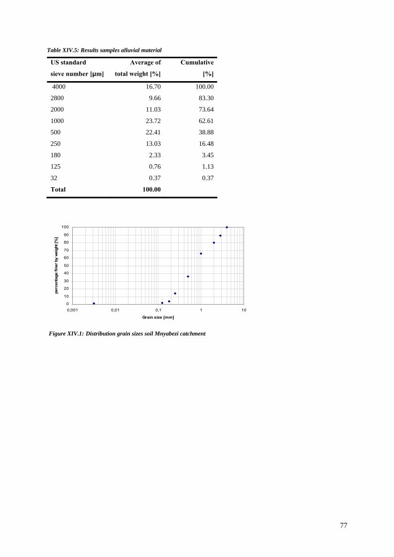
77
Table XIV.5: Results samples alluvial material
US standard
sieve number [μm]
Average of
total weight [%]
Cumulative
[%]
4000 16.70 100.00
2800 9.66 83.30
2000 11.03 73.64
1000 23.72 62.61
500 22.41 38.88
250 13.03 16.48
180 2.33 3.45
125 0.76 1.13
32 0.37 0.37
Total 100.00
0
10
20
30
40
50
60
70
80
90
100
0,001 0,01 0,1 1 10
Grain size [mm]
perc
enta
ge fi
ner b
y w
eigh
t [%
]
Figure XIV.1: Distribution grain sizes soil Mnyabezi catchment

78
Appendix XV: Dimension Mnyabezi reservoir Table XV.15: Coordinates of the Mnyabezi reservoir
GPS-point Latitude Longitude Y-projection UTM-grid* X-projection UTM-grid
1 S 21°48’73.2’’ E 29°07’21.7’’ 76.22.495 N 07.14.686 E
2 S 21°48’73.8’’ E 29°07’25.5’’ 76.22.488 N 07.147.26 E
3 S 21°48’68.9’’ E 29°07’32.8’’ 76.22.542 N 07.14.801 E
4 S 21°48’61.5’’ E 29°07’36.2’’ 76.22.623 N 07.14.838 E
5 S 21°48’53.6’’ E 29°07’33.6’’ 76.22.710 N 07.14.812 E
6 S 21°48’47.0’’ E 29°07’27.6’’ 76.22.785 N 07.14.751 E
7 S 21°48’38.3’’ E 29°07’19.8’’ 76.22.882 N 07.14.672 E
8 S 21°48’40.1’’ E 29°07’05.8’’ 76.22.864 N 07.14.526 E
9 S 21°48’57.7’’ E 29°07’07.9’’ 76.22.668 N 07.14.545 E
10 S 21°48’71.6’’ E 29°07’20.3’’ 76.22.514 N 07.14.672 E
11 S 21°48’71.9’’ E 29°07’23.2’’ 76.22.509 N 07.14.701 E
12 S 21°48’64.5’’ E 29°07’15.1’’ 76.22.592 N 07.14.619 E
13 S 21°48’59.2’’ E 29°07’14.7’’ 76.22.651 N 07.14.616 E
14 S 21°48’65.7’’ E 29°07’24.1’’ 76.22.578 N 07.14.588 E
15 S 21°48’56.5’’ E 29°07’26.7’’ 76.22.680 N 07.14.842 E
16 S 21°48’58.8’’ E 29°07’13.3’’ 76.22.654 N 07.14.787 E
17 S 21°48’60.3’’ E 29°07’36.4’’ 76.22.636 N 07.14.840 E
* the Y-projection is 300 m more south than the official map (BUVUMA 2129 A3) published by the Surveyor-General, Zimbabwe.
0714500E 0714600E 0714700E 0714800E
7622400N
7622500N
7622600N
7622700N
7622800N
7622900N
0714900E
Scale: UTM-GridDatum: WGS-84
100 m
N River
Reservoir 1m
1 2
3
4
5
6
78
9
10 11
12
1315
1617
14
Reservoir 0.75 m
Reservoir model 0.73 m
Reservoir model 1.00 m
Figure XV.1: Dimensions of the Mnyabezi reservoir

79
Appendix XVI: Dimension Bengu reservoir
Table XVI.1: Coordinates of the Bengu reservoir
GPS-point Latitude Longitude Y-projection UTM-grid* X-projection UTM-grid
1 S 21°30’304’’ E 29°02’586’’ 76.20.187 N 07.12.317 E
2 S 21°30’289’’ E 29°02’595’’ 76.20.232 N 07.12.344 E
3 S 21°30’295’’ E 29°03’013’’ 76.20.215 N 07.12.394 E
4 S 21°30’329’’ E 29°03’022’’ 76.20.110 N 07.12.420 E
5 S 21°30’361’’ E 29°03’004’’ 76.20.010 N 07.12.367 E
* the Y-projection is 300 m more south than the official map (BUVUMA 2129 A3) published by the Surveyor-General, Zimbabwe.
0712300E 0712400E 0712500E 0712600E
7620000N
7620100N
7620200N
7620300N
0712700E
Scale: UTM-GridDatum: WGS-84
100 m
N
River1
2
3
4
5
Reservoir
Reservoir model
Figure XVI.1: Dimensions Bengu reservoir
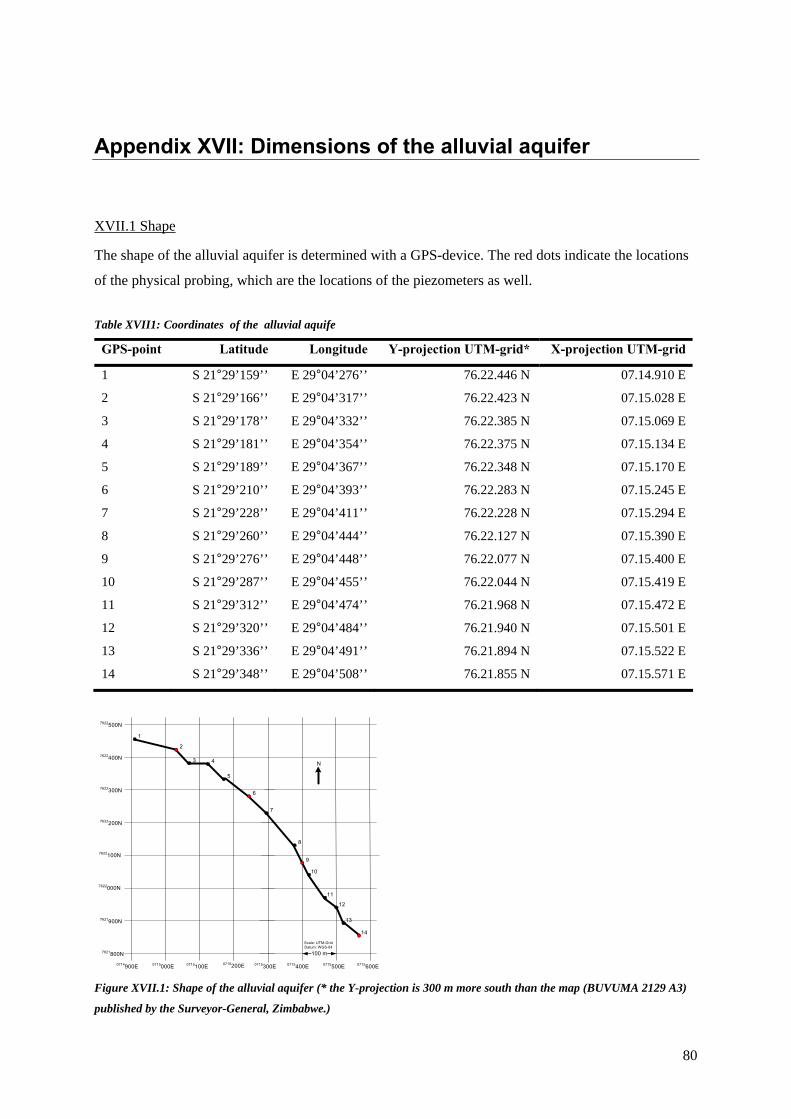
80
Appendix XVII: Dimensions of the alluvial aquifer
XVII.1 Shape
The shape of the alluvial aquifer is determined with a GPS-device. The red dots indicate the locations
of the physical probing, which are the locations of the piezometers as well.
Table XVII1: Coordinates of the alluvial aquife
GPS-point Latitude Longitude Y-projection UTM-grid* X-projection UTM-grid
1 S 21°29’159’’ E 29°04’276’’ 76.22.446 N 07.14.910 E
2 S 21°29’166’’ E 29°04’317’’ 76.22.423 N 07.15.028 E
3 S 21°29’178’’ E 29°04’332’’ 76.22.385 N 07.15.069 E
4 S 21°29’181’’ E 29°04’354’’ 76.22.375 N 07.15.134 E
5 S 21°29’189’’ E 29°04’367’’ 76.22.348 N 07.15.170 E
6 S 21°29’210’’ E 29°04’393’’ 76.22.283 N 07.15.245 E
7 S 21°29’228’’ E 29°04’411’’ 76.22.228 N 07.15.294 E
8 S 21°29’260’’ E 29°04’444’’ 76.22.127 N 07.15.390 E
9 S 21°29’276’’ E 29°04’448’’ 76.22.077 N 07.15.400 E
10 S 21°29’287’’ E 29°04’455’’ 76.22.044 N 07.15.419 E
11 S 21°29’312’’ E 29°04’474’’ 76.21.968 N 07.15.472 E
12 S 21°29’320’’ E 29°04’484’’ 76.21.940 N 07.15.501 E
13 S 21°29’336’’ E 29°04’491’’ 76.21.894 N 07.15.522 E
14 S 21°29’348’’ E 29°04’508’’ 76.21.855 N 07.15.571 E
0714900E 0715000E 0715100E
7621800N
7621900N
7622000N
7622100N
7622200N
7622300N
0715200E 0715400E 0715500E 0715600E
Scale: UTM-GridDatum: WGS-84
100 m
N
0715300E
7622400N
7622500N
1
2
3 4
5
6
7
8
9
10
11
12
13
14
Figure XVII.1: Shape of the alluvial aquifer (* the Y-projection is 300 m more south than the map (BUVUMA 2129 A3)
published by the Surveyor-General, Zimbabwe.)

81
XVII.2 Physical Probing
The physical probing is done at four lines along the alluvial aquifer. The probing started on the right
bank, while looking downstream.
Table XVI.2: Physical probing line 1
Point [m] Depth [m] Point [m] Depth [m]
0 0.00 5 0.97
2 1.02 6 0.85
3 1.30 7 1.00
4 1.30 9 0.00
Location line 1 120 m downstream dam Width of line 1 9 meter
Table XVII.3: Physical probing line 2
Point [m] Depth [m] Point [m] Depth [m]
0 0.00 6.5 0.66
0.5 0.42 8.5 0.63
2.5 0.98 10.5 0.00
4.5 0.87
Location line 2 370 m downstream dam Width of line 2 10.5 m
Table XVII.4: Physical probing line 3
Point [m] Depth [m] Point [m] Depth [m]
0 0.00 6 0.82
2 1.16 8 0.75
4 1.12 10 0.00
Location line 3 620 m downstream dam Width of line 3 10 m
Table XVII.5: Physical probing line 4
Point [m] Depth [m] Point [m] Depth [m]
0 0.00 5 0.89
1 0.64 7 1.00
3 0.89 9 0.00
Location line 4 900 m downstream dam Width of line 9 9 m
XVII.3 Resistivity test
The resistivity test is done at the same four lines along the alluvial aquifer as the physical probing.
Unfortunately, the reading for line 1 and 3 gave unrealistic results, so these are not presented here. The
location is measured from the right riverbank, while looking downstream.

82
Table XVII.6: Resistivity test line 2
Line 2 Location 2m Line 2 Location 4m
AB/2 [m] MN/2 [m] ρ [Ω.m] s.d. [%] AB/2 [m] MN/2 [m] ρ [Ω.m] s.d. [%]
1.5 0.5 257.22 0.1 1.5 0.5 123.33 0.1
2 0.5 158.05 0.1 2 0.5 78.94 0.2
2.5 0.5 97.43 0.1 2.5 0.5 52.54 0.0
3 0.5 71.73 1.1 3 0.5 44.58 0.1
5 0.5 55.30 0.2 5 0.5 40.98 0.0
7 2.0 50.18 0.3 7 2.0 49.25 0.5
10 2.0 70.83 1.1 10 2.0 52.36 0.2
15 2.0 81.88 3.1 15 2.0 60.93 1.9
Table XVII.7: Resistivity test line 4
Line 4 Location 3m Line 4 Location 7m
AB/2 [m] MN/2 [m] ρ [Ω.m] s.d. [%] AB/2 [m] MN/2 [m] ρ [Ω.m] s.d. [%]
1.5 0.5 397.48 0.3 1.5 0.5 529.09 0.3
2 0.5 74.39 7.7 2 0.5 280.07 0.1
2.5 0.5 2.5 0.5 124.39 0.1
3 0.5 87.80 0.7 3 0.5 62.01 0.7
5 0.5 79.27 1.1 5 0.5 67.16 1.2
7 2.0 147.72 0.0 7 2.0 61.14 0.9
10 2.0 158.42 0.5 10 2.0 78.89 2.2
15 2.0 142.44 4.3 15 2.0 56.59 6.6
10
100
1000
1 10 100
Depth [m]
Res
istiv
ity [O
hm. m
2 ]
line 2 - 2mline 4 - 3mline 2 - 4mline 4 - 7m
Figure XVII.2: Results resistivity test
XVII.4 Slope
The slope of the alluvial aquifer is determined with a dumpy level and a tape measure. The heights are
measured from the reference level 99.000, which represents the top of the gauging plate in the
reservoir.

83
Table XVII.8: Slope of the alluvial aquifer
Measuring
Point
Distance [m] Measured height [m] Difference in height [m] Slope [%]
1 0.00 95.043 0.082 0.259
2 31.65 94.961 0.090 0.424
3 21.25 94.871 0.070 0.307
4 22.80 94.801 0.048 0.162
5 29.61 94.753 0.150 0.595
6 25.22 94.603 - 0.009 - 0.035
7 25.44 94.612 0.120 0.490
8 24.50 94.492 0.060 0.002
9 30.00 94.432 0.068 0.273
10 24.90 94.364 0.038 0.141
11 26.93 94.326 0.110 0.409
12 26.93 94.216 0.047 0.173
13 27.10 94.169 0.082 0.259
Total 316.33 0.874 0.276

84
Appendix XVIII: Groundwater table data alluvial aquifer
Two piezometers per physical probing line were dug into the alluvial aquifer on the deepest points
according to the physical probing. Due to the pointed end of the piezometers the tapeline can not reach
the end of the piezometer, see Figure XVIII.1 and XVIII.2 for a representation of the field situation.
So a few cm per piezometer have to be added to calculate the water level. It was often not possible to
dig the piezometers in until the granite layer. The difference between the physical probing (the real
physical depth) and the depth of the piezometers is recorded. So, this height difference have to be
added to the water level as well. Piezometers 1, 2, 3, 4, 7 and 8 were pulled out of the alluvial aquifer
by kids on the 3rd of April. The piezometers were dug in on the 4th of April again. Due to this the depth
of the piezometers were changed. All the data according to the depth is given in Table XVIII.1. The
location is measured from the right riverbank, while looking downstream.
Figure XVIII.1: Piezometer (1) Figure XVIII.2: Piezometer (2) Table XVIII.1: Depth of the piezometers (from surface area of the alluvial aquifer)
Piezometer Location [m] Real depth
aquifer [cm]
Depth piezometer
until 3rd of April [cm]
Depth piezometer
after 3rd of April [cm]
1 3.0 130 109 104
2 7.0 100 70.5 75.5
3 2.5 98 91.5 93.5
4 4.5 87 71.5 67.5
5 4.0 82 77 77
6 6.0 112 93 93
7 3.0 89 86 80
8 7.0 100 97 89

85
The results of the measurements are given in Table XVIII.2. Some days are missing, because the field
assistant was not able to do the readings these days.
Table XVIII.2: Rough data from the piezometers in the alluvial aquifer
Number piezometer
Date 1 [cm] 2 [cm] 3 [cm] 4 [cm] 5 [cm] 6 [cm] 7 [cm] 8 [cm]
11-03-2007 8 2.4 20 22 29 0 30 0
12-03-2007 5 2.2 14.2 10 18 0 20 0
13-03-2007 3 1.2 13 7.5 13.6 0 15 0
14-03-2007 3 1 12.2 5 8.2 0 10 0
15-03-2007 0 0 5 1 2 0 3 0
16-03-2007 0 0 0 0 0 0 0 0
…
28-03-2007 0 0 0 0 0 0 0 0
29-03-2007 flow flow flow flow flow flow flow flow
30-03-2007 90 70 80 86.4 60.3 50.2 80 79
31-03-2007 80 65 69 70 50.5 49.3 72 70.2
01-04-2007 70 50 70.5 55.1 50 70 78 55
02-04-2007 - - - - - - - -
03-04-2007 - - - - - - - -
04-04-2007 40 60 58 28 30 20 11 39
05-04-2007 - - - - - - - -
06-04-2007 - - - - - - - -
07-04-2007 - - - - - - - -
08-04-2007 - - - - - - - -
09-04-2007 - - - - - - - -
10-04-2007 - - - - - - - -
11-04-2007 - - - - - - - -
12-04-2007 10 8 missing missing 9.3 16.2 6.3 16.2
13-04-2007 5 4.2 missing missing 5.1 10 3.1 11.1
14-04-2007 2 1 missing missing 3.1 4 2.1 5.3
15-04-2007 0 0 missing missing 2 3.1 2 1
16-04-2007 0 0 missing missing 0 0 0 0
17-04-2007 0 0 missing missing 0 0 0 0
18-04-2007 0 0 missing missing 0 0 0 0
19-04-2007 0 0 missing missing 0 0 0 0
20-04-2007 0 0 missing missing 0 0 0 0
21-04-2007 0 0 missing missing 0 0 0 0
…
04-05-2007 0 0 missing missing 0 0 0 0

86
In Table XVIII.3 the calculated results of the groundwater depth are given for the period from the 28th
of March until the 16th of April. In Figure XVIII.3 the data is visualized in a graph. Piezometer 3 and 4
are not presented, because the data suggest some reading errors and besides the last part is missing.
Table XVIII.3: Groundwater level in the alluvial aquifer (* estimates)
Number piezometer
Date 1 [cm] 2 [cm] 3 [cm] 4 [cm] 5 [cm] 6 [cm] 7 [cm] 8 [cm]
28-03-2007 0 0 0 0 0 0 0 0
29-03-2007 130 100 98 87 82 112 89 100
30-03-2007 116 94.5 84.5 105.9 65.3 69.2 89 90
31-03-2007 106 89.5 73.5 89.5 55.5 68.3 81 81.2
01-04-2007 96 74.5 75 74.6 55 59* 77* 66
02-04-2007 - - - - - - - -
03-04-2007 - - - - - - - -
04-04-2007 66 64.5* 62.5 47.5 35 39 40* 50
05-04-2007 - - - - - - - -
06-04-2007 - - - - - - - -
07-04-2007 - - - - - - - -
08-04-2007 - - - - - - - -
09-04-2007 - - - - - - - -
10-04-2007 - - - - - - - -
11-04-2007 - - - - - - - -
12-04-2007 36 32.5 missing missing 14.3 35.2 15.3 27.2
13-04-2007 31 28.7 missing missing 10.1 29 12.1 22.1
14-04-2007 28 25.5 missing missing 8.1 23 11.1 16.3
15-04-2007 26 24.5 missing missing 7 22.1 11 12
16-04-2007 24 23.5 missing missing 5 19 9 11
0
20
40
60
80
100
120
140
28-mrt 30-mrt 1-apr 3-apr 5-apr 7-apr 9-apr 11-apr 13-apr 15-apr 17-apr
Date [dd-mm]
Wat
er d
epth
[cm
]
Piezometer 1Piezometer 2Piezometer 5Piezometer 6Piezometer 7Piezometer 8
Figure XVIII.3: Groundwater level in the alluvial aquifer

87
Appendix IXX: Results dam overflow
1
10
100
1000
10000
100000
1000000
01-11-88 01-12-88 01-01-89 01-02-89 01-03-89 01-04-89 01-05-89 01-06-89 01-07-89 01-08-89 01-09-89 01-10-89 01-11-89
Date [dd-mm-yy]
Dam
ove
rflow
[m3.
day]
Figure IXX.1: Days over dam overflow for the Mnyabezi reservoir for the dry year ‘88/’89
1
10
100
1000
10000
100000
1000000
01-11-97 01-12-97 01-01-98 01-02-9801-03-98 01-04-98 01-05-98 01-06-98 01-07-98 01-08-98 01-09-98 01-10-98 01-11-98
Date [dd-mm-yy]
Dam
ove
rflo
w [m
3.da
y]
Figure IXX.2: Water level for the Mnyabezi reservoir for the normal year ‘97/’98
1
10
100
1000
10000
100000
1000000
01-11-96 01-12-96 01-01-97 01-02-9701-03-97 01-04-97 01-05-97 01-06-97 01-07-97 01-08-97 01-09-97 01-10-97 01-11-97
Date [dd-mm-yy]
Dam
ove
rflo
w [m
3.da
y]
Figure IXX.3: Days over dam overflow for the Mnyabezi reservoir for the wet year ‘96/’97
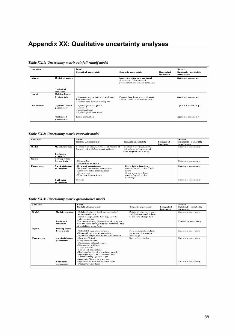
88
Appendix XX: Qualitative uncertainty analyses Table XX.1: Uncertainty matrix rainfall-runoff model
Table XX.2: Uncertainty matrix reservoir model
Table XX.3: Uncertainty matrix groundwater model