Embed Size (px)
Citation preview

2017
UNIVERSIDADE DE LISBOA
FACULDADE DE CIÊNCIAS
DEPARTAMENTO DE ENGENHARIA GEOGRÁFICA, GEOFÍSICA E ENERGIA
Potential of bifacial PV installation and its integration with
storage solutions
Sofia Carvalho Ganilha
Mestrado Integrado em Engenharia da Energia e do Ambiente
Dissertação orientada por:
Prof. Doutor Miguel Brito (FCUL)
Doutora Filipa Reis (EDP Inovação)

ii

iii
Agradecimentos
A presente dissertação representa o culminar de 5 anos de trabalho árduo e aprendizagem
constante, a qual não seria possível de realizar sem o apoio e orientação de várias pessoas. Por este
motivo, esta primeira página serve como agradecimento a todos os que direta e/ou indiretamente
estiveram envolvidos: o meu mais sincero OBRIGADA.
Em primeiro lugar, gostaria de expressar a minha eterna gratidão aos meus orientadores, o
professor Miguel Brito, a doutora Filipa Reis e o doutor André Botelho, não só pela disponibilidade
constante, a supervisão e orientação do trabalho realizado, mas também pelas soluções, ideias e
sugestões que surgiram em momentos que pareciam “becos sem saída”. Quero igualmente agradecer ao
professor Miguel Brito por me ter ensinado a “dar os primeiros passos” no grande mundo do fotovoltaico
e por ser um docente “outside the box” que cultiva nos seus alunos o mesmo espírito.
A seguir, quero agradecer à engenheira Joana Jacinto e ao doutor Mário Simões por terem feito
questão de acompanhar o meu trabalho, ajudando-me sempre que lhes foi solicitado, e por estarem
presentes em todas as reuniões de orientação.
À Sara Freitas, pela disponibilidade, pela simpatia contagiante, pela paciência que teve ao ensinar-
me a trabalhar num novo software e, especialmente, pelo altruísmo em partilhar o seu conhecimento.
Aos investigadores e especialistas em fotovoltaico bifacial, Dr. Matthieu Chiodetti e Dr. Radovan
Kopecek, que partiharam comigo o seu trabalho e prontamente responderam aos meus pedidos de ajuda.
Por último, quero agradecer àqueles que indiretamente me deram o suporte necessário para
finalizar a dissertação e sem os quais não seria a pessoa que sou hoje.
Aos meus mais-que-tudo, os meus pais Celestino e Maria João, que sempre apoiaram as minhas
decisões, que tiveram a paciência para suportar o meu mau humor em períodos de pressão e que me
deram o que precisava para seguir os meus sonhos.
À minha família, não de sangue, mas de coração, que eu escolhi e me criou desde bebé, e com
quem eu partilho todos os momentos da minha vida, bons e menos bons. Obrigada por me deixarem ser
uma “Cordeiro Serra”.
Ainda aos meus amigos de sempre, particularmente à Inês e à Sara, e aqueles que acompanharam
todo o meu percurso na faculdade e se tornaram amigos para sempre, em especial ao Filipe, ao Rafael,
à Filipa, ao Márcio e ao João Lopes.
Finalmente, o meu agradecimento ao Hugo Ventura, pelo amor e por me incentivar a sorrir em
todos os momentos.
iv
Resumo
O conceito de usar ambos os lados de um módulo solar fotovoltaico para converter a radiação
solar em energia elétrica surgiu no final do século XX e é conhecido como tecnologia bifacial
fotovoltaica. Para além da radiação incidente na parte frontal, as células solares bifaciais convertem a
radiação difusa, refletida e direta recebida pela superfície traseira e ativa da célula. Para tal, é necessário
que os módulos onde se encontram inseridas permitam a penetração da radiação em ambas as faces, o
que pode ser conseguido utilizando vidro temperado ou uma backsheet transparente. Este tipo de
tecnologia tem demonstrado grande potencial, sendo os ganhos bifaciais já reportados de algumas
instalações da ordem dos 30%.
De modo a quantificar o desempenho dos módulos bifaciais, três indicadores são utilizados. O
ganho bifacial de irradiância é a razão entre a irradiância intercetada pela parte traseira e frontal do
módulo, sendo que esta última pode ser interpretada como a irradiância total útil incidente num módulo
monofacial, ou seja, a que incide na sua superfície dianteira e é utilizada para a conversão em energia
elétrica. O ganho bifacial de energia é o quociente entre a energia convertida por um módulo bifacial e
aquela que é convertida por um módulo monofacial, ambas ponderadas pela área do painel solar. Por
último, dado que a potência instalada é atualmente mais valorizada do que a produção por unidade de
área efetiva instalada, utiliza-se também o ganho bifacial simples que é semelhante ao ganho bifacial de
energia, mas a energia convertida é ponderada pela potência nominal do módulo. Notar que se hoje o
preço dos módulos bifaciais é de alguma forma proporcional à potência, é de esperar que com economias
de escala possa ser proporcional à sua área.
A presente dissertação tem como principal objetivo analisar e avaliar as diferenças que estão
associadas à utilização de módulos fotovoltaicos bifaciais comparativamente à tecnologia monofacial
tradicional, tanto em termos de irradiância incidente como de produção de energia elétrica. Além disso,
é analisado como e quais os benefícios de integrar a tecnologia fotovoltaica bifacial com soluções de
armazenamento de forma a otimizar sistemas de autoconsumo para um consumidor típico residencial,
podendo este estar ou não conectado à rede elétrica.
Uma instalação bifacial é mais sensível à sua envolvente e à sua própria configuração do que um
sistema fotovoltaico monofacial. Por este motivo, a configuração ideal de um módulo bifacial é
investigada recorrendo a um software de modelação, Rhinoceros®, de forma a determinar o ângulo de
inclinação, elevação, posição de montagem e distância entre fileiras de módulos e entre módulos
adequados para maximizar quer o ganho bifacial de irradiância, quer a irradiância total que atinge ambas
as superfícies do módulo. Para além disso, também é estudada de que maneira a refletividade do solo
pode potenciar o ganho bifacial.
As modelações foram efetuadas com base nas características conhecidas da futura instalação da
EDP que tem como intuito testar módulos fotovoltaicos bifaciais. Os dados meteorológicos típicos de
Lisboa, Portugal, servem de base às simulações posteriores.
Os resultados mostram que, para uma instalação fotovoltaica típica, o ganho bifacial de irradiância
de um único módulo varia entre 37% e 45%, dependendo do ângulo de inclinação. O ângulo de
inclinação que maximiza o ganho bifacial de irradiância é geralmente maior do que o ângulo ótimo que
maximiza a radiação total intercetada. Módulos mais elevados e solos com maior refletividade
aumentam o ganho bifacial de irradiância. Também foi visto que a irradiação intercetada pelo lado
traseiro do módulo bifacial é mais homogénea no caso de este estar numa posição de paisagem e não

v
retrato, o que influencia a conversão em energia elétrica devido ao mismatch da corrente fotogerada por
cada célula solar bifacial.
Relativamente à simulação para um conjunto de módulos bifaciais, as distâncias ideais entre filas
e entre painéis numa mesma fila para minimizar a interferência entre eles são superiores ao caso
monofacial, e tanto maiores quanto mais refletivo for o solo.
O segundo objetivo da dissertação passa por desenvolver um modelo elétrico com base no qual
se pode estimar a produção dos módulos fotovoltaicos bifaciais. Para o efeito, considera-se que uma
célula bifacial pode ser representada eletricamente como duas células monofaciais em paralelo, cada
uma delas representada pelo circuito equivalente de um díodo. Este modelo foi desenvolvido recorrendo
ao software MATLAB® Simulink e foi testado para várias orientações, ângulos de inclinação e posições
de montagem.
A partir das simulações efetuadas, verificou-se que, para um módulo bifacial, o ganho bifacial de
energia é proporcional ao ganho bifacial de irradiância e ambos aumentam com a fração difusa. Para
uma instalação fotovoltaica típica da EDP, o ganho bifacial de energia varia entre 28% a 35%,
dependendo do ângulo de inclinação.
Se a orientação do módulo bifacial for diferente da ótima, isto é, se se encontrar orientado a este
ou oeste, é possível observar-se alterações da curva típica de produção fotovoltaica, nomeadamente o
aparecimento de dois picos, um de manhã e outro ao anoitecer.
Por último, foi avaliado o papel que os módulos bifaciais poderiam ter em soluções de
autoconsumo residencial. Os resultados mostram que os módulos solares bifaciais e monofaciais
orientados a sul se comportam de maneira semelhante, por unidade de potência instalada, pelo que o
maior investimento em sistemas bifaciais não se justifica. Porém, módulos bifaciais na vertical,
orientados a este ou oeste, permitem maior consumo de eletricidade gerada localmente, o que pode ser
vantajoso dado que a energia excedentária que se vende à rede não é tão lucrativa para o consumidor
como a que se deixa de comprar. Os módulos bifaciais na vertical permitem, em média, a redução de
cerca 1 kWh/kWp no sistema de baterias, comparativamente com módulos virados a sul e com inclinação
ótima, assegurando ainda assim uma taxa de autoconsumo superior a 90%.
Se a comparação entre módulos bifaciais e monofaciais considerar a área de implantação em
oposição à potência instalada, a utilização de painéis bifaciais verticais orientados a este ou oeste permite
não só aumentar a fração de energia autoconsumida em mais de 10%, relativamente a módulos bifaciais
com configuração ótima, mas também diminuir a capacidade do sistema de armazenamento necessária,
o que se traduz numa possível redução dos custos associados.
Se o sistema de autoconsumo estiver isolado da rede elétrica, a autossuficiência (i.e. fração das
necessidades energéticas do consumidor asseguradas pelo sistema de geração fotovoltaica) garantida
por módulos bifaciais orientados a sul é aproximadamente 7% superior à dos módulos monofaciais com
a mesma configuração, para a mesma capacidade nominal de armazenamento instalada (kWh).
Finalmente, verificou-se que para soluções de autoconsumo isoladas da rede elétrica, a
combinação de módulos fotovoltaicos bifaciais com diversas orientações, nomeadamente virados a sul,
a este e/ou oeste, permite obter uma taxa de autossuficiência mais elevada, podendo mesmo aproximar-
se dos 100% durante as horas solares se a área de módulos e a capacidade da bateria instaladas forem
suficientemente elevadas.
Palavras-Chave: Fotovoltaico Bifacial, Modelo de Irradiância, Modelo Elétrico, Autoconsumo,
Armazenamento

vi
Abstract
The concept of using both faces of a photovoltaic module to convert solar radiation into electrical
energy emerged at the end of the 20th century and is known as bifacial photovoltaics. Along with the
incident radiation on the front side, bifacial solar cells take advantage of the diffuse, reflected and direct
radiation that reaches the cell’s active rear side.
This dissertation focuses on evaluating and analysing the differences of using bifacial over
traditional monofacial photovoltaic technology, both in terms of collected irradiance and power
production. Also, it explores how to integrate this technology with storage to optimize self-consumption
solutions.
In this study, the optimum configuration for a bifacial photovoltaic module is investigated
numerically, using the software Rhinoceros and Simulink, in order to determine the suitable tilt angle,
elevation and mounting position of the module and the ground reflectivity that optimises bifacial gain.
Modelling a bifacial photovoltaic system for a case study, Lisbon, Portugal, showed that power
production is highly dependent on the incident radiation, stand design and reflectivity of the ground. For
a typical photovoltaic plant, the bifacial gain varies from 28%-35% for power production and from 37%-
45% for the irradiation received, depending on the tilt angle. Higher stands and more reflective ground
surfaces boost the bifacial gains. It is also shown that the electrical generation gain is proportional to the
irradiance gain and both increase with the diffuse fraction.
Finally, the analysis of a residential self-consumption solution that seeks to integrate a bifacial
photovoltaic installation and batteries showed that south-facing bifacial and monofacial modules behave
similarly, with similar yields per unit of power installed. Per unit module area, south facing bifacial solar
modules clearly outperform standard monofacial modules, since the self-sufficiency rate (i.e. fraction
of the energy demand that is fulfilled by on-site photovoltaic generation) can be approximately 7%
higher, for the same nominal capacity of the storage system (kWh).
Results also showed that, the combination of bifacial photovoltaic modules with different
orientations, namely south, east and/or west, allows a higher self-sufficiency rate that can almost reach
100% during solar hours, if the module area and storage capacity installed is high enough.
The use of bifacial modules in the vertical, orientated towards the east or the west, increases the
fraction of the self-consumed energy in more than 10%, decreasing the excess energy sold to the grid
and reducing the required storage capacity, which means the associated costs may be significantly
reduced.
Keywords: Bifacial Photovoltaic, Irradiance Model, Electrical Model, Self-consumption, Storage
vii
Contents
Agradecimentos ...................................................................................................................... iii
Resumo ................................................................................................................................... iv
Abstract ................................................................................................................................... vi
List of Figures ......................................................................................................................... ix
List of Tables ......................................................................................................................... xii
List of Notations, Abbreviations and Acronyms .................................................................. xiv
1. Introduction ..................................................................................................................... 1
1.1. Solar energy and photovoltaic technology .............................................................. 1
1.2. Motivation for bifacial PV ...................................................................................... 1
1.3. Research objectives ................................................................................................. 2
1.4. Dissertation outline ................................................................................................. 3
2. Overview of the bifacial concept ..................................................................................... 4
2.1. History of bifacial technology ................................................................................. 4
2.2. Bifacial PV technology ........................................................................................... 5
2.3. Working principles .................................................................................................. 7
2.4. Testing modules and standardization ...................................................................... 7
2.5. Bifacial market and associated costs ....................................................................... 8
2.6. Modelling a bifacial system .................................................................................. 10
2.6.1. Irradiance model ............................................................................................... 10
2.6.2. Bifacial cell model ........................................................................................... 12
2.6.2.1. Bifacial electrical model ............................................................................ 13
2.6.2.2. Thermal model ........................................................................................... 15
2.7. Vertical installations .............................................................................................. 16
3. Irradiance bifacial model ............................................................................................... 18
3.1. Methodology ......................................................................................................... 18
3.1.1. Optimization of a bifacial PV installation’s configuration ............................... 19
3.2. Results and discussion ........................................................................................... 21
3.2.1. Reference module configuration ...................................................................... 21
3.2.2. Optimization of the configuration for a single module .................................... 22
3.2.3. Optimization of the configuration for a PV stand ............................................ 26
4. Electrical bifacial model ................................................................................................ 31
4.1. Methodology ......................................................................................................... 31
4.1.1. Cell design ........................................................................................................ 31
viii
4.1.2. Thermal model ................................................................................................. 33
4.1.3. Model dynamics ............................................................................................... 34
4.1.4. Performance indicators ..................................................................................... 35
4.2. Results and discussion ........................................................................................... 36
4.2.1. Performance analysis ........................................................................................ 36
4.2.2. Externalities that affect the bifacial gain .......................................................... 42
5. Integration of bifacial PV with storage solutions .......................................................... 44
5.1. Methodology ......................................................................................................... 44
5.1.1. Self-consumption performance indicators ........................................................ 44
5.1.2. Load consumption profile ................................................................................ 45
5.1.3. Configuration of the PV installation ................................................................ 46
5.1.4. Self-consumption installation ........................................................................... 46
5.1.5. Model dynamics ............................................................................................... 47
5.2. Results and discussion ........................................................................................... 48
5.2.1. PV generation ................................................................................................... 48
5.2.2. Electricity consumption .................................................................................... 51
5.2.3. Self-consumption system dynamics ................................................................. 52
5.2.4. Self-consumption system performance ............................................................ 55
5.2.5. Ideal PV technology for a self-consumption solution ...................................... 58
6. Conclusion and further work ......................................................................................... 64
7. Bibliographic references ............................................................................................... 68
8. Annexes ......................................................................................................................... 72
Annex I – Deduction of the method to electrical characterize bifacial PV modules .......... 72
Annex II – Predicted IBG and annual incident irradiation for all the module configurations
and ground surfaces in study ......................................................................................................... 76
Annex III - PrismSolar® MODEL Bi60-343BSTC ............................................................ 86
Annex IV – Predicted energy yield for all the module configurations in study .................. 87
Annex V – Daily power density PV curve for the module’s configurations considered for
the self-consumption solution ....................................................................................................... 88
Annex VI – SSR and SCR for the module configurations and battery capacities in study. 89

ix
List of Figures
CHAPTER 2. Overview of the bifacial concept
Figure 2.1 - Schematic of bifacial solar cell’s architecture proposed by H. Mori. 1 is a n-type thick
silicon layer, 2 and 2’ are thin p-type layers, 3 is the negative electrode and 4 is the positive electrode
in contact with the connecting portion of the layers 2 and 2’. [5] ...................................................... 4
Figure 2.2 - Cumulative Bifacial PV Installed Capacity. Adapted from [14] .................................... 5
Figure 2.3 - Efficiency and Bifaciality of different bifacial solar cells according to the manufacturer
and the architecture. [6] ...................................................................................................................... 6
Figure 2.4 - Schematic of a bifacial module and the components of the incident radiation on both
sides of the module. ............................................................................................................................ 7
Figure 2.5 - Prevision of the world market share of bifacial solar cells and modules. [15] ............... 8
Figure 2.6 - Results of the simulation of LCOE and COO calculation for different technologies.
Adapted from [14] .............................................................................................................................. 9
Figure 2.7 - Geometry for determining the view-factor between the shaded and unshaded region of
the ground and the module rear surface. .......................................................................................... 11
Figure 2.8 - Single diode equivalent circuit for a monofacial solar cell. ......................................... 12
Figure 2.9 - Typical equivalent electrical circuit for a bifacial solar cell. ........................................ 13
Figure 2.10 - Absorption behaviour of a monofacial and bifacial cell and a silicon wafer. [42] ..... 15
Figure 2.11 – Example of a daily generated power curve for bifacial and monofacial modules with
specific orientations, using radiation data from Mito City [47]. ...................................................... 17
CHAPTER 3. Irradiance bifacial model
Figure 3.1 - Rendering of the Rhinoceros geometry for a single solar cell (a) and a PV module (b)
used for incident irradiance estimation. The dimensions are in cm. ................................................ 19
Figure 3.2 - Inter-row and within row spacings visual demonstration. ............................................ 21
Figure 3.3 - Modelled annual cumulative irradiation dependency on the tilt angle for the reference
bifacial module (elevation=1m; ground=white gravel; mounting=landscape; orientation=south).
Right axis shows irradiance bifacial gain (IBG). ............................................................................. 22
Figure 3.4 - Inhomogeneity of the radiation on the rear side for two different module’s mounting
positions (ground=white painted concrete; tilt=45º; elevation=0.15m). The solar radiant exposure
presented is for a year....................................................................................................................... 23
Figure 3.5 - Modelled annual cumulative rear irradiation dependency on the tilt angle for the
reference bifacial module (elevation=1m; mounting=landscape; orientation=south). ..................... 24
Figure 3.6 - Annual IBG as a function of the albedo for different tilt angles (left) and elevations
(right). (mounting=landscape; orientation=south) ........................................................................... 25
Figure 3.7 – Dependency of the annual rear cumulative irradiation (lines) and the IBG (dots) on the
elevation and ground surface (tilt=45º; mounting=landscape; orientation=south). ......................... 26
Figure 3.8 - Effect of the distance between rows in the inhomogeneity of the radiation in the front of
the array (left) and in the back (right). The solar radiant exposure presented is for a year. ............. 27
Figure 3.9 - Total irradiation loss difference between rows with bifacial PV modules. The same losses
for monofacial modules are represented by the dotted line (tilt=45º; elevation=1m;
mounting=landscape; orientation=south). ........................................................................................ 28
Figure 3.10 - Effect of the distance between the modules within rows in the inhomogeneity of the
rear radiation. The solar radiant exposure presented is for a year. ................................................... 29
Figure 3.11 - IBG difference within a row for different spacing between modules, considering the
reference module (tilt=45º; elevation=1m; orientation=south). ....................................................... 29

x
Figure 3.12 - Module's spacing dependency on elevation (left) and tilt angle (right) considering the
reference model (ground=white gravel; orientation=south). ............................................................ 30
CHAPTER 4. Electrical bifacial model
Figure 4.1 - Simulated monofacial (a) and bifacial (b) solar cells in Simulink®. The -C- block
represents the input of the hourly irradiance (W/m2) from MATLAB workspace and -BS- converts
the input signal to a physical signal. ................................................................................................ 32
Figure 4.2 - Representation of the cell connection path for the monofacial and bifacial PV modules
simulated. ......................................................................................................................................... 32
Figure 4.3 - Simulink electrical model of a PV module. .................................................................. 34
Figure 4.4 - Flowchart of the algorithm implemented in MATLAB to find the MPP. .................... 34
Figure 4.5 - Simulated annual power output for the reference bifacial and monofacial PV modules
(tilt=30º; elevation=1m; orientation=south; ground=white gravel). ................................................ 36
Figure 4.6 - Daily variation of the EBG and predicted power production for the reference module on
17/August (tilt=30º; elevation=1m; orientation=south; ground=white gravel). ............................... 37
Figure 4.7 - Hourly EBG for the reference bifacial module during one year (tilt=30º; elevation=1m;
orientation=south; ground=white gravel). A logarithmic scale is applied to the vertical axis for
visualization purposes. The black dots represent a divergent behaviour. ........................................ 38
Figure 4.8 - EBG in function of the correspondent hour. The black dots represent a divergent
behaviour. (tilt=30º; elevation=1m; orientation=south; ground=white gravel) ............................... 38
Figure 4.9 - Monthly evaluation of the PR for a single monofacial and bifacial modules with the
reference configuration (tilt=30º; elevation=1m; orientation=south; ground=white gravel). .......... 39
Figure 4.10 - Annual energy production estimation for monofacial and bifacial modules with the
reference configuration (elevation=1m; orientation=south; ground=white gravel). In the right vertical
axis is represented the IBG and EBG for the bifacial PV module. .................................................. 39
Figure 4.11 - Daily generated power curve for three bifacial modules with specific orientations and
tilt angles on 17/August (elevation=1m; ground=white gravel). ..................................................... 41
Figure 4.12 - Representation of the EBG as a function of the IBG for the bifacial reference module
(tilt=30º; elevation=1m; orientation=south; ground=white gravel). ................................................ 42
Figure 4.13 - Representation of the EBG as a function of the kd for the bifacial reference module.
The black dots represent a divergent behaviour. (tilt=30º; elevation=1m; orientation=south;
ground=white gravel). ...................................................................................................................... 43
CHAPTER 5. Integration of bifacial PV with storage solutions
Figure 5.1 - Annual consumption of the residential sector (profile C) during 2015 [65]. ............... 45
Figure 5.2 - Schematic representation of the main components and energy fluxes in a self-
consumption installation. ................................................................................................................. 47
Figure 5.3 - Flowchart of the algorithm implemented in MATLAB to model the dynamics of a self-
consumption with storage system. ................................................................................................... 48
Figure 5.4 - Simulated monthly mean power output normalized by the area for the modules’ types
and configurations analysed for a self-consumption solution. The mean values were calculated only
for the solar hours. ............................................................................................................................ 49
Figure 5.5 - PV specific daily production for: (a) 30º South Monofacial; (b) 30º South Bifacial; (c)
90º East Bifacial; and (d) 90º West Bifacial. ................................................................................... 51
Figure 5.6 - Annual hourly consumption diagram of a typical residential considered for the
simulation, throughout 2015. The red dots represent the standard deviation of the hourly energy
demand relatively to the monthly average. ...................................................................................... 51
Figure 5.7 - Daily hourly load diagram for the residence of the analysis. ....................................... 52

xi
Figure 5.8 - Self-consumption dynamic for a system with two 30º bifacial solar modules facing south
with 343 W each (17/August). ......................................................................................................... 53
Figure 5.9 - Self-consumption dynamic for a system with two 30º monofacial solar modules facing
South with 270 W each (17/August). ............................................................................................... 54
Figure 5.10 - Self-consumption dynamic for a system with two vertical bifacial solar modules facing
east with 343 W each (17/August). .................................................................................................. 55
Figure 5.11 - SSR in function of the installed PV power for different storage system's capacities,
considering 30º south-facing bifacial PV modules. ......................................................................... 56
Figure 5.12 - SCR in function of the installed PV power for different storage system's capacities. 57
Figure 5.13 - SSR in function of the PV module for different storage system's capacities: (a) 686 Wp
PV installed; (b) 2.06 kWp PV installed. .......................................................................................... 58
Figure 5.14 - SCR in function of the PV module for different storage system's capacities: (a) 686 Wp
PV installed; (b) 2.06 kWp PV installed. .......................................................................................... 59
Figure 5.15 - SSR in function of the PV module for different storage system's capacities, for an
installed PV area of 2.68 m2. ............................................................................................................ 60
Figure 5.16 - SCR in function of the PV module for different storage system's capacities, for an
installed PV area of 2.68 m2. ............................................................................................................ 61
Figure 5.17 – Mean average of the hourly SSR for the different modules’ types and configurations
considered, a storage capacity of 1 kWh/kWp and a PV installation area of 2.68 m2. ..................... 62
CHAPTER 8. Annexes
Figure 8.1 - PV power density daily production for: (a) 30º South Monofacial; (b) 30º South Bifacial;
(c) 90º East Bifacial; and (d) 90º West Bifacial. .............................................................................. 88

xii
List of Tables
CHAPTER 2. Overview of the bifacial concept
Table 2.1 - Empirically determined coefficients used to predict the module's temperature based on
the mounting mode and module type [45]. 1 The module is mounted on an open rack allowing air to
circulate freely around the module; 2 The module is mounted on a rack with little clearance between
the building surface and module’s back allowing little air to flow over the module back; 3 The module
is mounted directly to a building surface in a building-integrated PV (BIPV) application preventing
air from flowing over the module back. ........................................................................................... 16
CHAPTER 3. Irradiance bifacial model
Table 3.1 - Reflectance, specularity and roughness of the PV materials used in the model. [55] .. 19
Table 3.2 – Overall reflectivity in the RGB visible spectrum of certain ground surfaces according to
[55]. .................................................................................................................................................. 20
Table 3.3 - Optimum tilt angle according to the elevation of the PV module and the type of ground
surface (mounting=landscape; orientation=south). .......................................................................... 23
CHAPTER 4. Electrical bifacial model
Table 4.1 - Electrical parameters for the front and rear sides of the solar cell introduced in Simulink®.
.......................................................................................................................................................... 33
Table 4.2 - Annual energy generation and EBG for the reference module in a portrait and landscape
mounting position (tilt=30º; elevation=1m; orientation=south; ground=white gravel). .................. 40
CHAPTER 5. Integration of bifacial PV with storage solutions
Table 5.1 - Configurations of the PV modules tested to integrate in a PV system with storage. ..... 46
Table 5.2 – Specific and absolute energy yield for the modules’ types and configurations analysed
for the self-consumption solution. .................................................................................................... 50
CHAPTER 8. Annexes
Table 8.1 - Annual cumulative energy density for the front and rear sides of a landscape solar module
above asphalt and correspondent IBG. ............................................................................................. 76
Table 8.2 - Annual cumulative energy density for the front and rear sides of a portrait solar module
above asphalt and correspondent IBG. ............................................................................................. 77
Table 8.3 - Annual cumulative energy density for the front and rear sides of a landscape solar module
above white painted concrete and correspondent IBG. .................................................................... 78
Table 8.4 - Annual cumulative energy density for the front and rear sides of a portrait solar module
above white painted concrete and correspondent IBG. .................................................................... 79
Table 8.5 - Annual cumulative energy density for the front and rear sides of a landscape solar module
above grass and correspondent IBG. ................................................................................................ 80
Table 8.6 - Annual cumulative energy density for the front and rear sides of a portrait solar module
above grass and correspondent IBG. ................................................................................................ 81
Table 8.7 - Annual cumulative energy density for the front and rear sides of a landscape solar module
above grey tiles and correspondent IBG. ......................................................................................... 82
Table 8.8 - Annual cumulative energy density for the front and rear sides of a portrait solar module
above grey tiles and correspondent IBG. ......................................................................................... 83
Table 8.9 - Annual cumulative energy density for the front and rear sides of a landscape solar module
above white gravel and correspondent IBG. .................................................................................... 84

xiii
Table 8.10 - Annual cumulative energy density for the front and rear sides of a portrait solar module
above white gravel and correspondent IBG. .................................................................................... 85
Table 8.11 - Annual energy converted normalized by the area of the module - Energy Yield (kWh/m2)
- or by the peak power - Specific Yield (kWh/kWp) -, for all the module configurations considered
in the electrical model. ..................................................................................................................... 87
Table 8.12 - SSR for a self-consumption system depending on the storage capacity and the
configuration and area of the modules installed. .............................................................................. 89
Table 8.13 - SCR for a self-consumption system depending on the storage capacity and the
configuration and area of the modules installed. .............................................................................. 90

xiv
List of Notations, Abbreviations and Acronyms
BG Bifacial Gain
BOS Balance of System Costs
BSF Back Surface Field
COO Cost of Ownership
CPC Compound Parabolic Concentrators
DHI Diffuse Horizontal Irradiation
DoD Depth of Discharge
EBG Energy Bifacial Gain
FF Fill Factor
GHI Global Horizontal Irradiation
HIT Heterojunction with Intrinsic Thin layer
IBC Interdigitated Back Contact
IBG Irradiance Bifacial Gain
IR Infrared (radiation)
kd Diffuse fraction
LCOE Levelized Cost of Electricity
MPP Maximum Power Point
NOCT Normalized Operating Cell Temperature
PV Photovoltaic
PERC Passivated Emitter and Rear Cell
PERT Passivated Emitter, Rear Totally diffused
PR Performance Ratio
RES Renewable Energy Sources
RMSE Root Mean Square Error
SCR Self-Consumption Rate
SOC State-Of-Charge
SSR Self-Sufficiency Rate
STC Standard Test Conditions (Cell Temperature = 25ºC, Irradiance =
1000W/m2 and Air Mass 1.5)

xv
UPAC Units of Production for Self-Consumption

Potential of bifacial PV installation and its integration with storage solutions
Sofia Carvalho Ganilha 1
1. Introduction
This chapter briefly reviews the use of solar technologies, such as photovoltaic (PV), to provide
part of the electricity that humankind requires, and discusses the most relevant challenges and
opportunities for the development of bifacial PV. Then, it presents the main research objectives of this
dissertation and, finally, the outline of the document.
1.1. Solar energy and photovoltaic technology
The potential shortage of supply to the demand of fossil fuels, as well as the awareness to the
environmental impacts caused by their irresponsible and continuous use, has significantly increased the
growing interest on more efficient and eco-friendly alternative technologies to convert energy.
Photovoltaics is one of the solutions to break the bond once created with fossil fuels and has great
potential since the solar radiation is a clean, widely accessible and unlimited energy resource and can
address a substantial fraction of the world’s energy demand.
In 2016, PV registered a record annual growth rate of energy capacity, making up about 47%
among all Renewable Energy Sources (RES) and totalling a worldwide installed capacity of 303 GW
[1]. Despite the positive outlook, solar PV had an estimated share of only 1.5% of the global electricity
generation [1]. The Roadmap of Solar Photovoltaic foresees that PV will achieve a 16% share in the
global electricity mix by 2050 [2]. In order to reach the objective, it is necessary to reduce the PV capital
cost and, simultaneously, increase the generated electricity throughout the system’s lifetime.
Over the last few years, low-cost electricity has increasingly been provided by solar technologies,
owing to technological improvements, upgraded financial solutions, manufacturing economies of scale
and the expansion into new markets. The continuous research for high tech and materials to make PV
cost-effective led to the enrichment of the solar market with a more sophisticated knowledge and
efficient use of solar radiation.
The incorporation of bifacial solar cells into glass-glass or glass-transparent backsheet modules
is one of the emerging solutions to achieve higher throughput at lower costs. It not only enhances the
energy yield of a PV system over its lifetime and its durability (due to a more robust and reliable
encapsulation that reduces degradation over time), which allows a reduction of the Levelized Cost of
Electricity (LCOE) [3], but also facilitates its incorporation in many applications, e.g. optimizing self-
consumption solutions with storage, since these solar modules are able to peak-shift the typical PV
production curve.
1.2. Motivation for bifacial PV
Bifaciality opens a new world of possibilities for the traditional PV knowledge, encouraging new
investments and the search for a new paradigm.
Despite being relatively expensive, mainly because of the additional manufacturing steps, the
requirement for high quality silicon wafers and lacking the opportunities for economies of scale as
CHAPTER 1. Introduction
Sofia Carvalho Ganilha 2
standard PV modules do, bifacial technology continues to be investigated to develop more practical and
cost-effective solar cells able to take advantage of the incident radiation that reaches their both active
surfaces. The simplicity of the concept is attractive, especially because relevant improvements can be
achieved merely by adjusting the manufacturing process of advanced cell architectures, which are (in
most cases) intrinsically bifacial.
The valuable purpose of using bifacial PV is mainly justified by the energy conversion boost over
the system’s lifetime, which strongly depends on the installation configuration and location, and the
improved performance and durability. Furthermore, it also enables the Balance Of System (BOS) costs
reduction and, hence, the decrease of LCOE. BOS reduction is essentially justified by a decrease of the
required area to install the PV power plant and, consequently, the related costs.
In addition, bifacial has an obvious advantage over monofacial PV, since it occupies the same
physical area but converts relatively more solar energy into electricity. Consequently, bifaciality can be
used to face space limitations in highly populated places (e.g. building integrated PV) or the shortage of
suitable sites with a reasonable capacity potential.
Finally, it is important to mention that bifacial can be used in many other applications, even when
monofacial would underperform. For example, bifacial modules mounted vertically could be beneficial
in terms of increasing dispersed PV generation in space-limited self-consumption systems, since they
can easily meet the consumer energy demand peaks in the morning and evening. Besides, they can be
installed in multiple applications where single rows of solar modules are appropriate, such as railways
and highways, using both surfaces to produce energy.
Nevertheless, as any other new technology trying to enter the market and open roads for
widespread use, bifacial faces some challenges related to the inexistence of an international standard for
rating the bifacial electrical characteristics, the manufacturing challenges that results in higher modules’
prices and the absence of long-term data to testify the theoretically calculated energy boost. Lastly, there
is the necessity to devise a methodology to effortlessly and accurately predict the energy gains in outdoor
conditions.
The last point will be one of the main objectives of the present dissertation, which aims to provide
the basis for a future performance analysis of bifacial PV technology. Although the results of the
simulations performed are purely theoretical, they may be soon used for comparison with real
quantitative measurements of the future EDP outdoor facility to test bifacial PV.
1.3. Research objectives
This dissertation explores the potential of bifacial PV installations and its integration with storage
solutions. The objectives are three-fold:
i. To evaluate the bifacial PV’s gains,
ii. To suggest the system design that increases the advantage of bifaciality and,
iii. To analyse how to integrate this technology with storage solutions and quantify the
advantages comparatively to monofacial PV systems.
Potential of bifacial PV installation and its integration with storage solutions
Sofia Carvalho Ganilha 3
To achieve the proposed goals, the work was divided into the following tasks:
▪ Identify the most widely used models to evaluate the performance of bifacial PV;
▪ Analyse the irradiation gain of a bifacial PV module;
▪ Investigate the impacts of relevant factors in the design and geometry of a bifacial power plant,
e.g. tilt angle, elevation, ground’s albedo, mounting, intra-row spacing and distance between
rows;
▪ Develop a simulation strategy to estimate the energy output of a bifacial system;
▪ Sizing a PV system with storage for a residential consumer and analysing the ideal configuration
of the modules and the capacity of the battery.
1.4. Dissertation outline
The outline of this dissertation is as follows.
In chapter 2, a state-of-art overview is given, whereas the principles and challenges of the bifacial
PV technology are described as well as the models already proposed for the evaluation of its
performance.
Then, the dissertation is divided in three major chapters, according to each one of the subjects
analysed and the algorithms implemented. The case study and assumptions made are thoroughly
described as well as the simulation input data.
Namely, chapter 3 covers the methodology to predict the incident radiation that reaches both
surfaces of bifacial PV modules. The results are also presented, analysed and discussed, focusing on the
evaluation of the bifacial gain in terms of irradiance received comparatively to a monofacial PV module
and on the determination of the ideal system design and module configuration.
Chapter 4 focuses on the bifacial PV power production and how it is affected by some intrinsic
and extrinsic variables to the system itself. After the methodology’s description, the results are analysed
based on performance indicators and the influence of some variables on the electrical power production
is discussed.
The focus of chapter 5 is to size a residential self-consumption system with storage and analyse
its dynamics. The influence of the installed PV power/area and the storage capacity on the capacity to
fulfil the consumer energy demand is also determined.
Finally, in chapter 6, the main conclusions of the dissertation are drawn and some
recommendations for future work are given.

CHAPTER 2. Overview of the bifacial concept
Sofia Carvalho Ganilha 4
2. Overview of the bifacial concept
Over the past few years, the PV market and solar manufacturers have shown a renewed and strong
interest for bifacial technology. This chapter briefly presents the history and principles of bifacial PV
and discusses the most relevant challenges for its development, such as bankability, lack of
standardization, associated costs and the modelling and simulation of bifacial PV systems.
2.1. History of bifacial technology
The invention of the bifacial concept is a subject of doubt since it could have been created not to
take advantage of the incident radiation on both sides of the solar cell, but as a consequence of the
structure and properties of certain types of cells.
The first silicon solar cell was produced in Bell Labs, in 1954, with an n-type Interdigitated Back
Contact (IBC) structure [4]. The architecture of this cell allows it to be operated in bifacial mode with
two active surfaces. However, credit of the creation of bifacial solar cells goes to the Japanese expert H.
Mori [5] and the Russian scientists A.K. Zaitseva and O.P. Fedoseeva [6] who developed the same idea
independently. In 1960, H. Mori patented a solar cell with a collecting p-n junction on each side of a n-
type silicon wafer, forming a p+np+ structure, and describes the possibility of being double-sided
illuminated [7], as can be seen in Figure 2.1. Since then, the efficiency evolved from residual values to
21.3% at the front and 19.8% at the rear side [7].
Many researchers investigated and continue to develop bifacial PV technology. The number and
diversity of bifacial solar cell structures is large, with over 166 accumulated patents in 2016a [8]. The
path of bifacial design often crosses Heterojunction with Intrinsic Thin layer (HIT), Passivated Emitter
and Rear Cell (PERC) and Passivated Emitter, Rear Totally diffused (PERT) solar cells [6].
Since its conception, bifacial technology evolved and many applications were proposed to make
use of this innovative idea, including for example its integration in Russian satellites since the 70s [9].
The advantages of using bifacial cells in space instead of monofacial are the enhancement of incident
radiation from the Sun and Earth’s albedo and the lower infrared (IR) absorbance that leads to reduced
a The results were obtained for the search terms “bifacial” + “solar”.
Figure 2.1 - Schematic of bifacial solar cell’s architecture proposed by H. Mori. 1 is a n-type thick silicon layer, 2 and 2’ are
thin p-type layers, 3 is the negative electrode and 4 is the positive electrode in contact with the connecting portion of the
layers 2 and 2’. [5]
Potential of bifacial PV installation and its integration with storage solutions
Sofia Carvalho Ganilha 5
operating temperature. Nowadays there are still 10 kW bifacial modules installed at the International
Space Station, with a proven power generation increase of 10-20% [7].
In terrestrial applications, bifacial started to be used with flat mirrors and, later, with Compound
Parabolic Concentrators (CPC), directing sunlight towards the rear side. Only in the early 80s, it was
realized that bifacial solar cells were sensitive to natural or artificially enhanced albedo of the
environment. Commercial applications have so far been restricted to few niche areas, such as noise
barriers on Swiss railways and highways and some research facilities [9]. Still, because of their improved
performance and potential, bifacial cells have entered the PV industry and market, although with a
relatively low share.
The installation of the world’s first large scale bifacial PV power plant took place in Hokuto,
Japan, in 2013, with a total power of 1.25 MW. This plant has reported a bifacial gainb (BG) of 19.5%,
producing more than 1.2 MWh/kW/year [10]. Since then, other bifacial power plants were installed in
Chile (2.5 MW), in the USA (12.8 MW) [11] and the largest project to date in China (50 MW) [12].
Recently, the Dutch Tempress Systems B.V. inaugurated one of Europe’s largest bifacial PV facilities
in Netherlands with 400 kW [13].
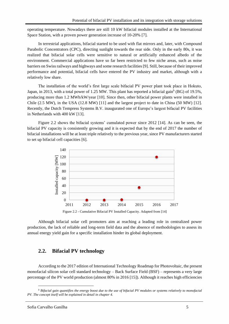
Figure 2.2 shows the bifacial systems’ cumulated power since 2012 [14]. As can be seen, the
bifacial PV capacity is consistently growing and it is expected that by the end of 2017 the number of
bifacial installations will be at least triple relatively to the previous year, since PV manufacturers started
to set up bifacial cell capacities [6].
Although bifacial solar cell promoters aim at reaching a leading role in centralized power
production, the lack of reliable and long-term field data and the absence of methodologies to assess its
annual energy yield gain for a specific installation hinder its global deployment.
2.2. Bifacial PV technology
According to the 2017 edition of International Technology Roadmap for Photovoltaic, the present
monofacial silicon solar cell standard technology – Back Surface Field (BSF) – represents a very large
percentage of the PV world production (almost 80% in 2016 [15]). Although it reaches high efficiencies
b Bifacial gain quantifies the energy boost due to the use of bifacial PV modules or systems relatively to monofacial
PV. The concept itself will be explained in detail in chapter 4.
0
20
40
60
80
100
120
140
2011 2012 2013 2014 2015 2016 2017
Inst
alle
d c
apac
ity [
MW
]
Figure 2.2 - Cumulative Bifacial PV Installed Capacity. Adapted from [14]

CHAPTER 2. Overview of the bifacial concept
Sofia Carvalho Ganilha 6
(up to 19% at the module level), its performance is limited by recombination at the rear surface and,
consequently, it is essential to develop new approaches to produce solar cells with higher efficiencies.
A running high efficiency alternative is double-sided contact cell concepts which are intrinsically
bifacial [15].
The main difference between conventional monofacial structures and a bifacial cell is that, in the
latter, the rear surface must have metal contacts instead of being fully covered by metal (usually an
aluminum-based paste). As a result, radiation can be collected both from the front and rear surfaces of
the solar cell.
When a PV manufacturer choses to go bifacial, the technical choice is essentially among three
structures: HIT, PERT and PERC, each one with different bifaciality levels. Bifaciality is defined as the
ratio between the rear side efficiency and the front side efficiency or as the ratio of the power output at
STC from the rear side upon the power output at STC from the front side.
Bifaciality =𝜂𝑟𝑒𝑎𝑟
𝜂𝑓𝑟𝑜𝑛𝑡 =
𝑃𝑆𝑇𝐶,𝑟𝑒𝑎𝑟
𝑃𝑆𝑇𝐶,𝑓𝑟𝑜𝑛𝑡 (2.1)
n-PERT and HIT are the most effective since they have a bifaciality of more than 90%, followed by
PERC with 70% [6]. Bifaciality depends strongly on the type of cell as seen in Figure 2.3.
As for the bifacial PV modules, the opaque backsheet must be replaced by an additional glass
layer or by an UV-resistant transparent backsheet. Although this type of encapsulation increases the
thermal insulation on the back side, bifacial cells still have a lower absorbance relatively to IR radiation,
which decreases the temperature of operation comparatively to monofacial PV modules. Besides, it
prevents the penetration of water in the module’s interior and reduces degradation over time, increasing
the duration of the module [9]. In the case of glass-glass modules, the package is also more rigid, which
reduces de mechanical stress on cells [16]. Although these advantages might not be sufficient to switch
the typical encapsulation of PV modules (regardless of technology), they come for free in bifacial PV
modules, since their rear surface must ensure that the incident radiation can reach the back side of the
bifacial PV cells.
In addition, the design of stable mounting systems and junction boxes should be changed to not
disturb the light-sensitive areas causing undesirable shading. Furthermore, the junction boxes must
handle higher currents [17], [9], [6].
Eff
icie
ncy
[%
] Bifaciality
[%]
Figure 2.3 - Efficiency and Bifaciality of different bifacial solar cells according to the manufacturer and the architecture. [6]

Potential of bifacial PV installation and its integration with storage solutions
Sofia Carvalho Ganilha 7
2.3. Working principles
Along with the incident radiation on the front side, bifacial PV take advantage of the diffuse,
reflected and direct radiation that reach the module’s active rear side, depending on its orientation,
elevation and tilt, site’s characteristics and the position of the sun in the sky, Figure 2.4. Thus, the power
output of the rear side is highly dependent upon the local ground’s albedo and its surroundings, the
module installation configuration and meteorological conditions. From the shadow region on the
ground, only diffuse radiation is captured by the solar module, while in the unshaded area, both direct
and diffuse radiation are reflected, affecting the rear side of the bifacial module.
When considering a PV stand, the evaluation of bifacial gains becomes more complex due to the
different variables involved, not only the aforementioned ones, but also the packing density (distance
between and within rows), the shadows produced by the mounting, the additional shading caused by the
neighbouring modules and the obstruction of reflected radiation. These considerations make bifacial PV
power plants more sensitive to the installation layout than the traditional ones that integrate monofacial
modules.
2.4. Testing modules and standardization
Making an accurate prediction of the annual yield of a PV stand and setting the system design
requires a precise and standardized electrical characterization of the solar modules in use. All PV solar
cells are characterized by a normalized operating curve obtained under Standard Test Conditions (STC),
which correspond to a normal irradiance of 1000 W/m2, an operating temperature of 25 ºC and an Air
Mass of 1.5, this allows a fair comparison between the many structures and commercial cells.
Characterizing bifacial solar cells is much more challenging because of the contribution of the
rear side’s power production to the measurements. There is no commonly accepted procedure to
consider this extra input which affects the estimation of the solar module’s performance.
Some companies are reporting bifacial PV by flashing the front side of the module with 1.1 suns
and taping the rear side with a black foil, others are reporting independently the values for both sides of
the module obtained at STC by covering one of the surfaces with a non-reflective sheet while
illuminating the other one [18]. It was also proposed the simultaneous measurements of both sides with
a double-sun simulator [19] and quoting the I-V parameters under different rear illumination conditions
[9], which indirectly assesses the interference between both sides.
Figure 2.4 - Schematic of a bifacial module and the components of the incident radiation on both sides of the module.
Direct and Diffuse
Diffuse
Reflected
Reflected
CHAPTER 2. Overview of the bifacial concept
Sofia Carvalho Ganilha 8
Despite all this procedural diversity, the PV community is making an effort to set international
testing standards for bifacial modules and lifetime testing conditions [21]. This is a step that can
contribute to increase the mass production and deployment of bifacial modules. The “IEC 60904-1-2:
Measurement of current-voltage characteristics of bifacial photovoltaic devices” initiated in 2016 is
expected to be published in 2018, after the ongoing revision [6].
Besides the obvious consequences of the lack of standardization of the characterization of bifacial
PV modules’ performance, it can also be difficult to develop an analytical and electrical model for
bifacial PV, since the current and voltage characteristics of the cell are considered as an input, as will
be seen in the chapter 4. Also, the indoor characterization is not appropriated to predict the outdoor
output of the module due to the inhomogeneous irradiation on the rear side that results in distortions in
the I-V curve, often altered by the effect of the module’s by-pass diodes [20].
2.5. Bifacial market and associated costs
The biggest barrier for bifacial PV is the high associated costs related to the cells’ manufacturing
and their integration in solar modules, which is one of the main reasons why bifacial has been a
technology for niche applications and with a low market share (2% in 2016 [15]).
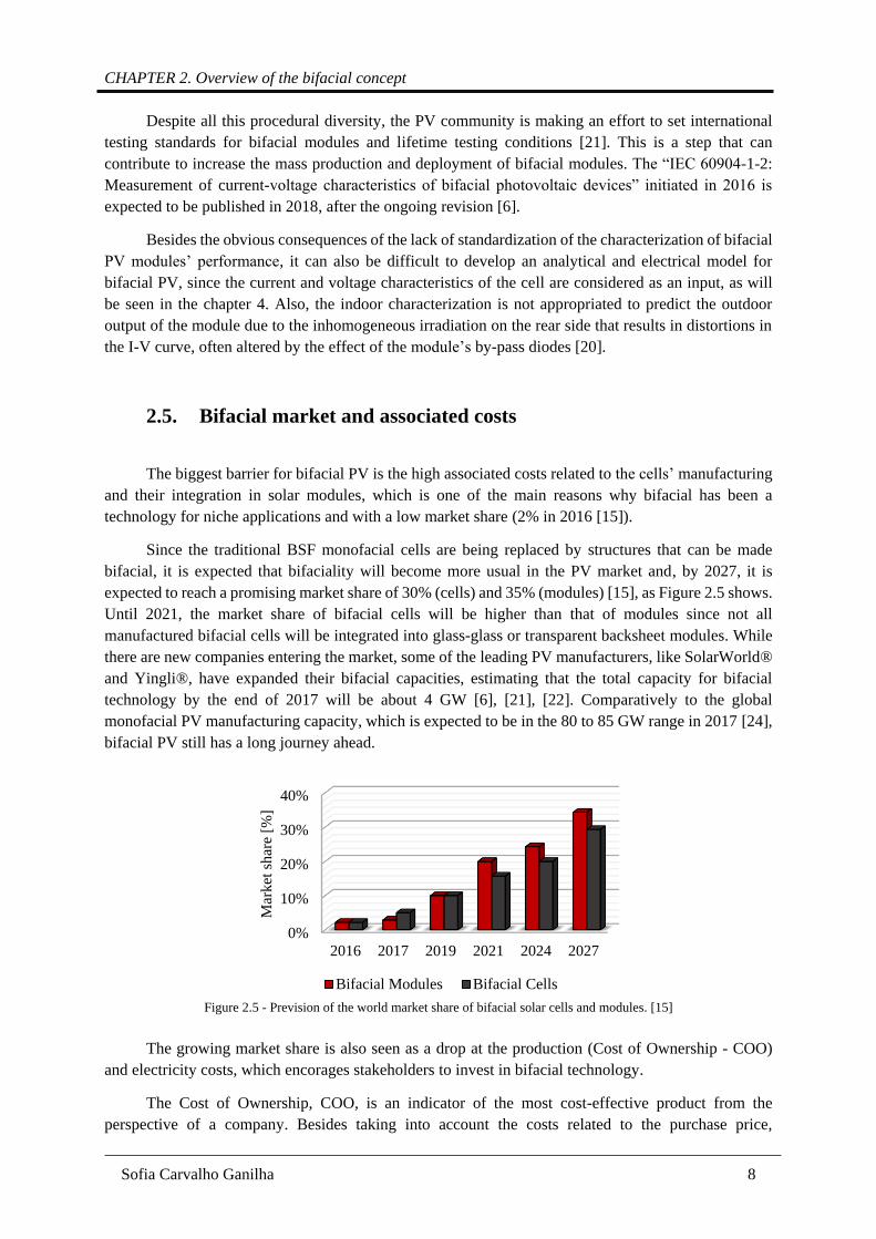
Since the traditional BSF monofacial cells are being replaced by structures that can be made
bifacial, it is expected that bifaciality will become more usual in the PV market and, by 2027, it is
expected to reach a promising market share of 30% (cells) and 35% (modules) [15], as Figure 2.5 shows.
Until 2021, the market share of bifacial cells will be higher than that of modules since not all
manufactured bifacial cells will be integrated into glass-glass or transparent backsheet modules. While
there are new companies entering the market, some of the leading PV manufacturers, like SolarWorld®
and Yingli®, have expanded their bifacial capacities, estimating that the total capacity for bifacial
technology by the end of 2017 will be about 4 GW [6], [21], [22]. Comparatively to the global
monofacial PV manufacturing capacity, which is expected to be in the 80 to 85 GW range in 2017 [24],
bifacial PV still has a long journey ahead.
The growing market share is also seen as a drop at the production (Cost of Ownership - COO)
and electricity costs, which encorages stakeholders to invest in bifacial technology.
The Cost of Ownership, COO, is an indicator of the most cost-effective product from the
perspective of a company. Besides taking into account the costs related to the purchase price,
0%
10%
20%
30%
40%
2016 2017 2019 2021 2024 2027
Mar
ket
shar
e [%
]
Bifacial Modules Bifacial Cells
Figure 2.5 - Prevision of the world market share of bifacial solar cells and modules. [15]
Potential of bifacial PV installation and its integration with storage solutions
Sofia Carvalho Ganilha 9
maintenance and operation, this tool also takes the product quality and the failure costs into
consideration [24].
The Levelized Cost Of Electricity, LCOE, is the cost per unit of the electricity produced by a
system and includes its total life cycle costs, such as the investment, the operation and maintenance
costs, etc. It provides an economic assessment to compare various RES with electricity prices. The
LCOE’s calculation of a PV system requires a record of the total electricity produced during the useful
lifetime and information about the financing, operation and maintenance costs, which are still
unaddressed data for bifacial PV. Also, the price of the energy generated by PV that is marketed can
vary significantly between countries due to the taxes and feed-in tariffs, reason why these are sometimes
omitted from the analysis [14].
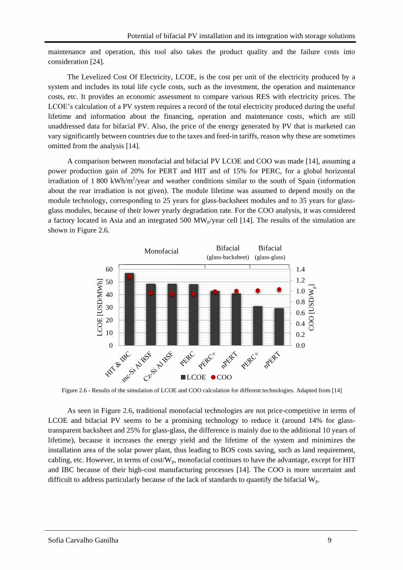
A comparison between monofacial and bifacial PV LCOE and COO was made [14], assuming a
power production gain of 20% for PERT and HIT and of 15% for PERC, for a global horizontal
irradiation of 1 800 kWh/m2/year and weather conditions similar to the south of Spain (information
about the rear irradiation is not given). The module lifetime was assumed to depend mostly on the
module technology, corresponding to 25 years for glass-backsheet modules and to 35 years for glass-
glass modules, because of their lower yearly degradation rate. For the COO analysis, it was considered
a factory located in Asia and an integrated 500 MWp/year cell [14]. The results of the simulation are
shown in Figure 2.6.
As seen in Figure 2.6, traditional monofacial technologies are not price-competitive in terms of
LCOE and bifacial PV seems to be a promising technology to reduce it (around 14% for glass-
transparent backsheet and 25% for glass-glass, the difference is mainly due to the additional 10 years of
lifetime), because it increases the energy yield and the lifetime of the system and minimizes the
installation area of the solar power plant, thus leading to BOS costs saving, such as land requirement,
cabling, etc. However, in terms of cost/Wp, monofacial continues to have the advantage, except for HIT
and IBC because of their high-cost manufacturing processes [14]. The COO is more uncertaint and
difficult to address particularly because of the lack of standards to quantify the bifacial Wp.
Figure 2.6 - Results of the simulation of LCOE and COO calculation for different technologies. Adapted from [14]
Monofacial
0.0
0.2
0.4
0.6
0.8
1.0
1.2
1.4
0
10
20
30
40
50
60
CO
O [
US
D/W
p]
LC
OE
[U
SD
/MW
h]
LCOE COO
Bifacial
(glass-backsheet)
Bifacial
(glass-glass)

CHAPTER 2. Overview of the bifacial concept
Sofia Carvalho Ganilha 10
2.6. Modelling a bifacial system
The potential of bifacial technology has been demonstrated by simulations and measurements not
only for single modules, where energy boosts between 5% [25] up to 54% [26] have been reported, but
also for small and larger PV stands, with reported power output increments between 5% and 25% [27],
depending on the size of the system. However, these references from literature refer to small systems
and the success of bifacial technology depends on demonstrating the same gains on larger scale PV
power plants. Bankability, which is the collection of real-world existing bifacial energy-yield data, is
one of the challenges that bifacial PV technology has to face in order to facilitate its wider deployment
[14].
For a given installation, it is fundamental to accurately predict the energy production and the
Bifacial Gain (BG) expected for the various possible stand geometries and different solar cells’
architectures.
The BG is defined as the ratio between the surplus energy produced by bifacial PV and the energy
yield of standard monofacial PV, calculated using the following equation.
Bifacial Gain (BG) =𝑒𝑏𝑖−𝑒𝑚𝑜𝑛𝑜
𝑒𝑚𝑜𝑛𝑜 (2.2)
Where 𝑒𝑏𝑖 is the energy yield of bifacial PV and 𝑒𝑚𝑜𝑛𝑜 is the energy yield of standard monofacial
PV. The BG can also be calculated in terms of specific yield (Wh/Wp).
The modelling of bifacial PV systems requires the development of a suitable irradiance model as
well as a specific electrical model of the bifacial PV modules.
2.6.1. Irradiance model
The irradiance model is required for the prediction of the incident irradiance on the front and rear
surfaces of the solar module.
Modelling a bifacial PV system is complex, mostly because the estimation of rear radiation not
only depends on correlated variables, such as the location, ground’s albedo and design of the stand, but
also due to uneven incident light (caused by shadings of the mounting structure, junction boxes, module
frames, irregular reflectors and even the neighbouring modules in the same array). Thus, the model must
consider the externalities imposed by the installation’s design, the environment and the shading of the
ground and its albedo, and is typically based on two distinct approaches.
The “View-Factor Method” calculates the radiation “emitted” from the underlying surface and
received by each cell. The ground beneath the module is divided into two parts: the shaded and unshaded
region; in the former only diffuse radiation is reflected, while in the latter both direct and diffuse
radiation are reflected. Coding this method is complex, since the view-factors must be calculated for
every instant (the position and shape of the shadow change with time due to the motion of the Sun in
the sky), it depends on the distance between each cell and the reflective surface and the inhomogeneity
caused by the mounting structure cannot be evaluated straightforwardly [11].

Potential of bifacial PV installation and its integration with storage solutions
Sofia Carvalho Ganilha 11
Numerically, the view-factor is defined as a geometric quantity that determines the fraction of
radiation leaving a surface A1 that directly impinges surface A2. It depends on the relative orientation
and distance between the two surfaces and, for finite surfaces, is given by
𝑉𝑖𝑒𝑤 𝐹𝑎𝑐𝑡𝑜𝑟𝐴1→𝐴2 =1
𝐴1∫ ∫
𝑐𝑜𝑠𝜃1 × 𝑐𝑜𝑠𝜃2
𝜋𝑟2𝑑𝐴2𝑑𝐴1
𝐴2𝐴1
(2.3)
Where 𝑟 is the distance between the differential areas 𝑑𝐴1 and 𝑑𝐴2 and 𝜃1 and 𝜃2 are the angles between
the normal vectors of the surfaces and the line that connects 𝑑𝐴1 and 𝑑𝐴2, respectively.
EDF R&D applied this model to a single module [26]. After calculating the view-factors between
the illuminated ground and the module and between the shadowed ground and the module, the total
irradiance on the rear surface is given by the flux of direct, diffuse and reflected irradiance (both from
the shaded and unshaded regions). The mean error varied between 1% and 3%, depending on the
configurations considered and the irradiance level, but the absolute error reached almost 15%, when
compared with measured data. Applying the same model to a string of modules resulted in a Root Mean
Square Error (RMSE) of 18.9 W/m2, i.e. 14% relatively to the mean of the measured values [28].
At the Sandia PV facility constructed in 2016 for testing bifacial PV modules, the back-surface
irradiance was also modelled by the “View-Factor Method” for cells installed near the middle of each
row, at the top and bottom of the module. Considering only the rear irradiance, the RMSE varied
between 4.8 W/m2 and 16.5 W/m2, being the deviation of the measured value from the modelled value
higher for the top cells [29].
The same approach was used by a partnership between ISC Konstanz and some universities in
Germany [30], [31] and J. Appelbaum from the School of Electrical Engineering in Israel [32] to
determine the input to the electrical model.
The second approach is called “Ray-tracing Method” and uses a 3D modelling software with a
daylighting and energy modelling plug-in. The simulation tool provides a precise and realistic rendering
of the PV system and radiation map distribution and can calculate the reflections between surfaces based
in their reflectivity. Commonly, the software uses an illumination model based on Perez model for direct
and diffuse irradiance that assumes the sky is isotropic for all weather conditions and all module’s
orientations [33]. It was tested, for example, by a group of researchers from NREL, Iowa University and
Sandia National Laboratories [34] and by Fraunhofer Institute for Solar Energy Systems [27]. EDF
calculated the RMSE of the method as 15.7 W/m2 which was found to be close to the pyranometers’
uncertainties [35].
Figure 2.7 - Geometry for determining the view-factor between the shaded and unshaded region of the ground and the
module rear surface.
CHAPTER 2. Overview of the bifacial concept
Sofia Carvalho Ganilha 12
For simple cases, there is a good agreement between the two methods [35], but as the complexity
increases, their pros and cons become more noticeable. For the “View-Factor Method”, as the size of
the system becomes larger and there are more externalities to take into account (e.g. structures that cause
shading, as the module frame and the mounting assembly), the processing time and complexity
increases. As for the “Ray-tracing Method”, it offers a great flexibility and accuracy in the prediction of
the incident irradiance, it also allows the representation of several configurations, surface properties and
considers the impact of inhomogeneous radiation, reflection and shading. Nevertheless, the
computational representation of the system cannot be generalized to every PV stand or location, i.e. it
is not universal, since it must reliably represent the real system, assuming it is already implemented,
which may not be the case.
2.6.2. Bifacial cell model
The rear and front radiation estimated by the irradiance model will be directly introduced as an
input in the electrical model to obtain the simulated bifacial power production. The system’s
characteristics that englobe the details of the module performance and the system installation are also
included in the electrical model.
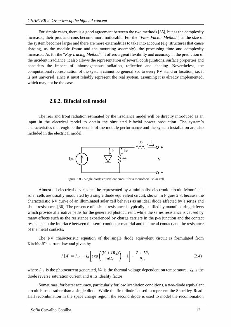
Almost all electrical devices can be represented by a minimalist electronic circuit. Monofacial
solar cells are usually modulated by a single diode equivalent circuit, shown in Figure 2.8, because the
characteristic I-V curve of an illuminated solar cell behaves as an ideal diode affected by a series and
shunt resistances [36]. The presence of a shunt resistance is typically justified by manufacturing defects
which provide alternative paths for the generated photocurrent, while the series resistance is caused by
many effects such as the resistance experienced by charge carriers in the p-n junction and the contact
resistance in the interface between the semi-conductor material and the metal contact and the resistance
of the metal contacts.
The I-V characteristic equation of the single diode equivalent circuit is formulated from
Kirchhoff’s current law and given by
𝐼 [𝐴] = 𝐼𝑝ℎ − 𝐼0 [exp ((𝑉 + 𝐼𝑅𝑠)
𝑛𝑉𝑇) − 1] −
𝑉 + 𝐼𝑅𝑠
𝑅𝑠ℎ (2.4)
where 𝐼𝑝ℎ is the photocurrent generated, 𝑉𝑇 is the thermal voltage dependent on temperature, 𝐼0 is the
diode reverse saturation current and 𝑛 its ideality factor.
Sometimes, for better accuracy, particularly for low irradiation conditions, a two-diode equivalent
circuit is used rather than a single diode. While the first diode is used to represent the Shockley-Read-
Hall recombination in the space charge region, the second diode is used to model the recombination
Figure 2.8 - Single diode equivalent circuit for a monofacial solar cell.

Potential of bifacial PV installation and its integration with storage solutions
Sofia Carvalho Ganilha 13
processes, such as Shockley-Read-Hall and Auger, elsewhere, in the base and emitter or in the front and
rear surfaces [37].
2.6.2.1. Bifacial electrical model
Different electrical models of bifacial solar cells have been proposed, developed and tested to
predict its power production output. Most of the models developed consider that a bifacial solar cell can
be represented as two monofacial cells in parallel, represented by the single diode or two-diodes
equivalent circuit. The electrical diagram of the model is presented in Figure 2.9.
The number of possible combinations for the incident radiation at the front and rear sides of a
bifacial module is virtually infinite, so it is neither practical nor feasible to determine the electrical
parameters of the PV module for all those conditions.
J. Singh et al. have synthesized a method to electrically characterize bifacial PV modules for all
illumination conditions [38]. The basis is the one-diode model of a monofacial cell and the electrical
parameters given as an input to the model are extracted from the I-V curves obtained independently for
the front and rear sides of the cell at STC. Therefore, the interference between both sides is not
considered, which can lead to slight deviations between the experimental data and the simulation results.
These extracted parameters include the short circuit currents, 𝐼𝑠𝑐,𝑓𝑟𝑜𝑛𝑡 and 𝐼𝑠𝑐,𝑟𝑒𝑎𝑟, and open circuit
voltages, 𝑉𝑜𝑐,𝑓𝑟𝑜𝑛𝑡 and 𝑉𝑜𝑐,𝑟𝑒𝑎𝑟, for front and rear sides of the bifacial solar cell, respectively.
The method assumes a linear response of the short circuit current for different radiation levels and
considers bifacial as a monofacial module operating at a current which is the sum of the currents
generated independently by the front and rear sides, because once the charge carriers have been
generated, it makes no difference to the cell from which side the incident radiation entered. In order to
define some parameters, the model also defines the irradiance ratio as the ratio of rear and front
irradiances, as following [38]:
𝐼𝑟𝑟𝑎𝑑𝑖𝑎𝑛𝑐𝑒 𝑅𝑎𝑡𝑖𝑜 (𝜒) =𝐺𝑟𝑒𝑎𝑟
𝐺𝑓𝑟𝑜𝑛𝑡 (2.5)
where 𝐺𝑟𝑒𝑎𝑟 and 𝐺𝑓𝑟𝑜𝑛𝑡 are the incident irradiances on the rear and front sides, respectively.
The power of bifacial modules can be defined as follows:
𝑃𝑏𝑖𝑓𝑎𝑐𝑖𝑎𝑙 = 𝐼𝑠𝑐,𝑏𝑖 𝑉𝑜𝑐,𝑏𝑖 𝐹𝐹𝑏𝑖 (2.6)
Figure 2.9 - Typical equivalent electrical circuit for a bifacial solar cell.
CHAPTER 2. Overview of the bifacial concept
Sofia Carvalho Ganilha 14
with 𝐼𝑠𝑐,𝑏𝑖, the short circuit current for bifacial modules, defined using the notion of short circuit current
gain (ℛ𝐼𝑠𝑐) relative to monofacial PV:
𝐼𝑠𝑐,𝑏𝑖 = ℛ𝐼𝑠𝑐 𝐼𝑠𝑐,𝑓𝑟𝑜𝑛𝑡 = (1 + 𝜒
𝐼𝑠𝑐,𝑟𝑒𝑎𝑟
𝐼𝑠𝑐,𝑓𝑟𝑜𝑛𝑡) 𝐼𝑠𝑐,𝑓𝑟𝑜𝑛𝑡 (2.7)
The bifacial open circuit voltage, 𝑉𝑜𝑐,𝑏𝑖, is
𝑉𝑜𝑐,𝑏𝑖 = 𝑉𝑜𝑐,𝑓𝑟𝑜𝑛𝑡 +(𝑉𝑜𝑐,𝑟𝑒𝑎𝑟 − 𝑉𝑜𝑐,𝑓𝑟𝑜𝑛𝑡)ln (ℛ𝐼𝑠𝑐
)
ln (𝐼𝑠𝑐,𝑟𝑒𝑎𝑟 − 𝐼𝑠𝑐,𝑓𝑟𝑜𝑛𝑡) (2.8)
And the bifacial fill factor, 𝐹𝐹𝑏𝑖 is
𝐹𝐹 𝑏𝑖 = 𝑝𝐹𝐹 − ℛ𝐼𝑠𝑐
𝑉𝑜𝑐,𝑓𝑟𝑜𝑛𝑡
𝑉𝑜𝑐,𝑏𝑖(𝑝𝐹𝐹 − 𝐹𝐹𝑓𝑟𝑜𝑛𝑡) (2.9)
In Equation 2.9, 𝑝𝐹𝐹 is the pseudo Fill Factor (FF) of the module considering no series resistance loss
which can be calculated using Equation 2.10.
𝑝𝐹𝐹 =(𝐼𝑠𝑐,𝑟𝑒𝑎𝑟/𝐼𝑠𝑐,𝑓𝑟𝑜𝑛𝑡)𝐹𝐹𝑓𝑟𝑜𝑛𝑡 − (𝑉𝑜𝑐,𝑟𝑒𝑎𝑟/𝑉𝑜𝑐,𝑓𝑟𝑜𝑛𝑡)𝐹𝐹𝑟𝑒𝑎𝑟
(𝐼𝑠𝑐,𝑟𝑒𝑎𝑟/𝐼𝑠𝑐,𝑓𝑟𝑜𝑛𝑡) − (𝑉𝑜𝑐,𝑟𝑒𝑎𝑟/𝑉𝑜𝑐,𝑓𝑟𝑜𝑛𝑡) (2.10)
This method has been shown to estimate the power output within 1% of measured results, for
different sets of irradiance conditions [43]. Its demonstration can be found in Annex I – Deduction of
the method to electrical characterize bifacial PV modules.
A collaborative investigation developed by ISC Konstanz and University of Stuttgart used a
simplified version of the model suggested by Singh et al., considering FF as a fixed value measured at
STC, which leads to an overestimation of the output power for high irradiance levels and an
underestimation for low irradiance levels. Although the good agreement between the measured and
simulated BG proves the reliability of the model, the authors defend that the simulation tool requires
some improvements, which include quantifying the daily and seasonal variation of ground’s albedo
(counting the influence of the diffuse fraction and the solar zenith angle), develop a more accurate
electrical model and considering shadowing effects [30].
The aforementioned analytical model gives accurate modulation for homogeneous irradiance
conditions, but it does not take into account the possible electric current mismatch in different cells in
the module due to the inhomogeneous patterns of intercepted radiation. Besides, the temperature of a
cell can also influence the power production and this effect is not included in the model. These
conditions are difficult to address analytically with the previous model without being onerous and time-
consuming. For this reason, numerical PV simulation software has been used to predict the enhanced
output of bifacial modules dates since 1993 [39].
P. Dupeyrat et al. developed a bifacial solar cell electrical model on Modelica/Dymola® based
on the two-diode approach. This model was used to study the influence of the tilt angle and several
albedos in three different locations. The results indicate that the BG in terms of energy yield is highly
dependent on the aforesaid variables, and the higher values are obtained for places where the global
irradiance is predominantly diffuse and installations with more reflective underlying surfaces. [26]

Potential of bifacial PV installation and its integration with storage solutions
Sofia Carvalho Ganilha 15
C. Reise and A. Schmid also used a PV simulation tool developed by Fraunhofer ISE to model,
simulate and validate the equivalent electrical system of a bifacial solar cell. The method produced quite
precise results with measured BG reaching 21.9%, while the modelled value reached 21.1%. [27]
The simulators and approaches used are diverse and generally need to account the specifications
of the system, the connection to the grid, the neighbouring environment and the module’s temperature
[31], [40], [41].
2.6.2.2. Thermal model
The thermal behaviour of a solar cell strongly influences its electrical performance. Hence, to
obtain a more reliable prediction of the annual energy yield, the temperature of the bifacial cells must
be calculated and, when possible, measured. The temperature of any solar cell is determined by the
energy balance between the absorbed radiation that is not converted in electrical energy and the heat lost
to the environment in form of convection and radiation.
Although the encapsulation (glass or transparent backsheet) increases the thermal insulation, the
fact that bifacial cells are almost transparent to infrared radiation leads to lower operating temperatures
and a corresponding increase of the power output. Figure 2.10 shows the difference in absorption of a
bifacial and monofacial cell above 1000 nm, but considering that this range only represents 20% of the
energy of AM 1.5, the absortion difference betweem the two technologies becomes about 6.5% [42]. It
was also shown that bifaciality does not affect the thermal properties of the cell and has only a slightly
effect on the voltage of the module [43].
Most PV manufacturers specify the Normalized Operating Cell Temperature (NOCT) which is
the temperature of a PV module under 800 W/m2, wind speed of 1 m/s (almost no convection) and
ambient temperature of 20ºC. The formula to calculate the cell temperature based on NOCT is the
following:
𝑇𝑐𝑒𝑙𝑙 = 𝑇𝑎𝑚𝑏𝑖𝑒𝑛𝑡 +𝑁𝑂𝐶𝑇 − 20°𝐶
800 𝑊/𝑚2× 𝐺 (2.11)
where 𝐺 is the irradiance in the solar cell plane (W/m2) and 𝑇𝑎𝑚𝑏𝑖𝑒𝑛𝑡 is the ambient temperature
measured (ºC).
However, NOCT is obtained for a “nude” module with free air circulation, which means it does
not include information about the mounting mode and the value is only slightly dependent on the
Figure 2.10 - Absorption behaviour of a monofacial and bifacial cell and a silicon wafer. [42]
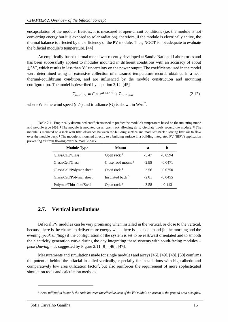
CHAPTER 2. Overview of the bifacial concept
Sofia Carvalho Ganilha 16
encapsulation of the module. Besides, it is measured at open-circuit conditions (i.e. the module is not
converting energy but it is exposed to solar radiation), therefore, if the module is electrically active, the
thermal balance is affected by the efficiency of the PV module. Thus, NOCT is not adequate to evaluate
the bifacial module’s temperature. [44]
An empirically-based thermal model was recently developed at Sandia National Laboratories and
has been successfully applied to modules mounted in different conditions with an accuracy of about
±5°𝐶, which results in less than 3% uncertainty on the power output. The coefficients used in the model
were determined using an extensive collection of measured temperature records obtained in a near
thermal-equilibrium condition, and are influenced by the module construction and mounting
configuration. The model is described by equation 2.12. [45]
𝑇𝑚𝑜𝑑𝑢𝑙𝑒 = 𝐺 × 𝑒𝑎+𝑏×𝑊 + 𝑇𝑎𝑚𝑏𝑖𝑒𝑛𝑡 (2.12)
where W is the wind speed (m/s) and irradiance (G) is shown in W/m2.
Table 2.1 - Empirically determined coefficients used to predict the module's temperature based on the mounting mode
and module type [45]. 1 The module is mounted on an open rack allowing air to circulate freely around the module; 2 The
module is mounted on a rack with little clearance between the building surface and module’s back allowing little air to flow
over the module back; 3 The module is mounted directly to a building surface in a building-integrated PV (BIPV) application
preventing air from flowing over the module back.
Module Type Mount a b
Glass/Cell/Glass Open rack 1 -3.47 -0.0594
Glass/Cell/Glass Close roof mount 2 -2.98 -0.0471
Glass/Cell/Polymer sheet Open rack 1 -3.56 -0.0750
Glass/Cell/Polymer sheet Insulated back 3 -2.81 -0.0455
Polymer/Thin-film/Steel Open rack 1 -3.58 -0.113
2.7. Vertical installations
Bifacial PV modules can be very promising when installed in the vertical, or close to the vertical,
because there is the chance to deliver more energy when there is a peak demand (in the morning and the
evening, peak shifting) if the configuration of the system is set to be east/west orientated and to smooth
the electricity generation curve during the day integrating these systems with south-facing modules –
peak shaving – as suggested by Figure 2.11 [9], [46], [47].
Measurements and simulations made for single modules and arrays [46], [49], [48], [50] confirms
the potential behind the bifacial installed vertically, especially for installations with high albedo and
comparatively low area utilization factorc, but also reinforces the requirement of more sophisticated
simulation tools and calculation methods.
c Area utilization factor is the ratio between the effective area of the PV module or system to the ground area occupied.

Potential of bifacial PV installation and its integration with storage solutions
Sofia Carvalho Ganilha 17
Vertically installed bifacial modules reduce soiling and snow accumulation, which decrease
cleaning costs. Also, it is possible to integrate bifacial PV in balconies [48] or in a vertical facade, for
example through a double skin configuration, which is practical since facades have a large collection
area and this structure can also provide a solution for natural or forced ventilation. However, the risk of
shading in an urban environment is higher [49].
For self-consumption solutions, the storage system is used to provide the energy in need when
there is not enough radiation to ensure the load’s necessities. If the installation uses a combination of
bifacial and monofacial PV modules with a very specific layout, the storage capacity of the battery’s
bank can be potentially lower than a system that only uses monofacial south orientated PV modules.
Another advantage is the bifaciality concept itself, since the bifacial modules convert more energy
occupying the same physical area as monofacial modules, the number of PV modules installed and the
area-related costs might decrease for the residential user.
However, the integration of this technology with storage solutions for self-consumption purposes
have not been analysed yet and is one of the main objectives of this dissertation work. The last task will
focus on sizing the storage capacity based on the load profile, the system characteristics and the bifacial
PV power production.
Figure 2.11 – Example of a daily generated power curve for bifacial and monofacial modules with specific orientations,
using radiation data from Mito City [47].

CHAPTER 3. Irradiance bifacial model
Sofia Carvalho Ganilha 18
3. Irradiance bifacial model
In the current chapter, the basis of the irradiance bifacial model developed in this dissertation is
presented. Primarily, the methodology implemented and the assumptions made are described. Then, the
influence of some relevant factors, which are associated to the configuration of a bifacial PV module
and system, on the intercepted radiation is analysed. The ideal designs to favour bifaciality and to ensure
the maximization of the radiation collected are suggested.
3.1. Methodology
The Typical Meteorological Year (TMY) data for Lisbon (38.73ºN, -9.15ºW) forms the basis of
the irradiance model. The data representative of the long-term average climatic conditions is extracted
from the EnergyPlus® database [51]. It contains yearly information about the global and diffuse
horizontal irradiation (GHI and DHI, respectively), dry bulb temperature, wind velocity and relative
humidity.
The irradiance model uses the “Ray-tracing Method” approach, in which the TMY data will be
an input in the 3D modelling software, Rhinoceros® [52]. Using a daylighting and energy modelling
plug-in, DIVA® [53], the program computes a complete sky radiance distribution based on Perez model
and a cumulative sky approach [54], based on any pair of GHI and DHI.
The Irradiance Bifacial Gain (IBG) is defined as the ratio of the rear side contribution (difference
between the radiation intercepted by a bifacial and a monofacial module) to the front side over a certain
time, as shown in Equation 3.1. This variable is used for comparison and it is not a module property, so
each system layout needs to be assessed individually.
𝐼𝐵𝐺 =𝐺𝑏𝑖𝑓𝑎𝑐𝑖𝑎𝑙 − 𝐺𝑚𝑜𝑛𝑜𝑓𝑎𝑐𝑖𝑎𝑙
𝐺𝑚𝑜𝑛𝑜𝑓𝑎𝑐𝑖𝑎𝑙=
𝐺𝑟𝑒𝑎𝑟
𝐺𝑓𝑟𝑜𝑛𝑡 (3.1)
To analyse the IBG of a stand-alone south-facing module, a bifacial solar module inspired on
standardized measurements was designed in Rhinoceros® as two parallel collections of 60 cells in
opposite directions. Each cell has an effective area of 223 cm2 corresponding to 15×15 cm, as shown in
Figure 3.1 (a). The total area of the PV module is approximately 1.34 m2. The support structure and
junction box were not considered to allow the extrapolation of the results to all modules and mounting
structures, however, this will overestimate the incident radiation and, consequently, the energy yield.

Potential of bifacial PV installation and its integration with storage solutions
Sofia Carvalho Ganilha 19
The optical properties, such as reflectivity, roughness and specularity, of the cells, frame and
silver strings were defined according to the database of materials provided by Singapore University of
Technology and Design [55] and are listed in Table 3.1. The detail allows the model to take into
consideration the interaction of the frame with the intercepted radiation and how this affects the
illumination profile of the PV cells.
Table 3.1 - Reflectance, specularity and roughness of the PV materials used in the model. [55]
Material Total Reflectance (%) Specularity (%) Roughness (%)
Frame 4.75 0.62 0
Silver Strips 31.9 21.1 0
PV Cell 3.87 2.99 0
The irradiance analysis was made for the total radiation received over a typical year both for a
monofacial and a bifacial PV modules to allow the comparison between them. The model output consists
in the energy density (kWh/m2) obtained by 70 light sensors equidistantly distributed over the analysis
surface.
3.1.1. Optimization of a bifacial PV installation’s configuration
The irradiance model is used not only to determine the IBG of bifacial PV relatively to
monofacial, but also to optimize the configuration of the bifacial power plant that enhances the collection
of radiant energy in absolute terms.
Bifacial PV systems are more sensitive to the stand configuration and neighbouring characteristics
than standard monofacial PV systems. There are some key factors that need to be addressed in order to
determine the most efficient configuration for a single module or power plant. The annual energy yield
depends on the latitude, the ground’s albedo, the elevation of the module, its tilt angle, the mounting
and the distances between the modules within the same row and between arrays.
(a) (b)
Figure 3.1 - Rendering of the Rhinoceros geometry for a single solar cell (a) and a PV module (b) used for incident
irradiance estimation. The dimensions are in cm.

CHAPTER 3. Irradiance bifacial model
Sofia Carvalho Ganilha 20
Albedo dependency
The albedo is a property of a non-luminous surface that describes the ratio between the reflected
and the incident radiation. In order to simulate outdoor surface materials with different albedos, the
optical properties were defined using the database of Singapore University [55]. The ground surfaces
selected cover a wide range of reflectivity (listed in Table 3.2) and are the most common materials in
PV applications. Although the surface’s albedo was considered constant, it has spectral and directional
dependencies that vary with time [56].
Table 3.2 – Overall reflectivity in the RGB visible spectrum of certain ground surfaces according to [55].
Surface type Overall Reflectivity (%)
Asphalt 8.2
Grass 10.4
Grey Tiles 45.5
White Gravel 44.0
White Painted Concrete 82.4
Elevation of the module
The elevation is defined as the distance between the ground, assumed flat, and the lowest edge of
the module. This variable has also a great influence on the bifacial energy yield. The elevations analysed
were 0.15 m (placing the modules too close to the reflective surface enhances self-shading, thus reducing
the radiation available on the rear side [57]), 0.5 m, 1 m, 1.5 m and 2 m.
Tilt angle
The tilt angle influences the fraction of the sky and ground “seen” by the front and rear sides of
the module and, consequently, the irradiation intercepted by them. Tilt angles from 0º to 90º were
analysed within a 15º interval.
Landscape vs. portrait module
The mounting position of the module may be landscape (i.e. the longer edge is parallel to the
ground) or portrait (i.e. the shorted edge is parallel to the ground). The chosen layout will be relevant
for electric current mismatch in different cells/strings in the module due to the patterns of inhomogeneity
of the intercepted radiation.
Inter-row and within row spacing
After the ideal values for the aforesaid parameters have been determined for a single module, the
next step is to evaluate the configuration of a bifacial PV plant, which is expected to be negatively
affected by the presence of adjacent modules in the same row or in the front and back queues that can
cause mutual-shading and lead to a decrease of the total incident radiation, particularly on the rear side.

Potential of bifacial PV installation and its integration with storage solutions
Sofia Carvalho Ganilha 21
Consequently, the availability of rear surface irradiance for a bifacial PV stand depends upon inter
and within rows spacings (Figure 3.2). These were also analysed to determine the optimal configuration
for the system, considering their relationship with other variables already enunciated. The simulations
for the row-to-row distance considered the range from 1 m (minimum spacing for maintenance of the
modules) to 4 m, and the distance between modules within a row – intra-row spacing – was changed
from 0 to 2 m with an interval of 0.5 m.
3.2. Results and discussion
The environment, ground reflectivity and design of the system have a great influence on the
energy yield of a bifacial PV stand. The impacts are now analysed in the subsequent sections. It is
important to remember that results are expected to be slightly overestimated, since the mounting
structure and the junction box were not considered.
3.2.1. Reference module configuration
For readability, results are presented considering a reference bifacial PV system configuration
that is set according to the information known about the bifacial PV plants being installed.
It will be located in mainland Portugal, with a ground surface of white gravel, the module's
elevation will be about 1 m and the tilt angle will be 30º.
Although the portrait mounting is more typical for PV modules, the reference system has
landscape modules, which is the configuration of the modules in EDP facilities that will be used to
validate the theoretical results obtained, albeit not in time of this dissertation.
Figure 3.3 presents the annual cumulative energy density determined for bifacial solar modules
facing south for the climatic conditions of Lisbon, with an elevation of 1 m, in a landscape mounting
and a white gravel ground (the reference configuration). The results show that the optimal tilt angle is
found to be about 41º, which maximizes not only the global irradiation but also the rear energy density
intercepted annually. Despite all tilt angles were simulated, the comparisons made to study the irradiance
received and the optimal configuration for a bifacial PV stand were done using a more practical reference
slope of 45º, which is very close to the mean tilt angle that maximizes the yearly radiation received by
the module.
Figure 3.2 - Inter-row and within row spacings visual demonstration.

CHAPTER 3. Irradiance bifacial model
Sofia Carvalho Ganilha 22
It may be noticed that the angle that maximizes the IBG is 90º, since the annual cumulative energy
density of a monofacial module is relatively small when compared to the rear side. This happens because
IBG only informs about how much more irradiation a bifacial module receives than a monofacial.
However, to specify an optimum tilt angle, the interest will always be in maximizing the overall
irradiation received.
It can also be noticed that the amplitude and variation of the annual cumulative energy density
for the rear side with the tilt angle of the module is much lower when compared to the front side.
Consequently, the front side is decisive for the quantification of the total solar energy received and
intercepted by the PV module.
The annual cumulative irradiation received by the front and rear surfaces, as well as the IBG, are
presented in Annex II – Predicted IBG and annual incident irradiation for all the module configurations
and ground surfaces in study, for all the module configurations and ground surfaces studied.
3.2.2. Optimization of the configuration for a single module
Landscape vs. portrait module
In the rear side of the module, the irradiation intercepted is more inhomogeneous than in the front
side, which will result in a cell mismatch. Since the cells are connected in series in most bifacial modules,
this inhomogeneity is expected to affect the total output of the module.
The uniformity of the radiation received by the rear side of the module is related to its landscape
or portrait mounting and elevation. The non-uniformity of solar radiant exposure is larger for portrait
modules with lower elevation, as shown in Figure 3.4. Both mounting positions were simulated over
different conditions. The simulations for a single module gave the same results except for the case of a
solar module close to the ground in the presence of a highly reflective surface. In this situation, the IBG
is higher for the portrait case due to the bigger portion of reflected radiation captured (the portion of the
39%37% 37% 38% 41%
45%
0%
10%
20%
30%
40%
50%
0
500
1000
1500
2000
2500
3000
15 30 45 60 75 90
IBG
[%
]
Ann
ual
cu
mula
tiv
e en
erg
y d
ensi
ty
[kW
h/m
²]
Tilt [°]
Front Rear Total IBG
Figure 3.3 - Modelled annual cumulative irradiation dependency on the tilt angle for the reference bifacial module
(elevation=1m; ground=white gravel; mounting=landscape; orientation=south). Right axis shows irradiance bifacial gain
(IBG).
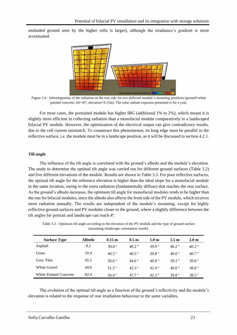
Potential of bifacial PV installation and its integration with storage solutions
Sofia Carvalho Ganilha 23
unshaded ground seen by the higher cells is larger), although the irradiance’s gradient is more
accentuated.
For most cases, the portraited module has higher IBG (additional 1% to 2%), which means it is
slightly more efficient in collecting radiation than a monofacial module comparatively to a landscaped
bifacial PV module. However, the optimization of the electrical output can give contradictory results,
due to the cell current mismatch. To counteract this phenomenon, its long edge must be parallel to the
reflective surface, i.e. the module must be in a landscape position, as it will be discussed in section 4.2.1.
Tilt angle
The influence of the tilt angle is correlated with the ground’s albedo and the module’s elevation.
The study to determine the optimal tilt angle was carried out for different ground surfaces (Table 3.2)
and five different elevations of the module. Results are shown in Table 3.3. For poor reflective surfaces,
the optimal tilt angle for the reference elevation is higher than the ideal slope for a monofacial module
in the same location, owing to the extra radiation (fundamentally diffuse) that reaches the rear surface.
As the ground’s albedo increases, the optimum tilt angle for monofacial modules tends to be higher than
the one for bifacial modules, since the albedo also affects the front side of the PV module, which receives
more radiation annually. The results are independent of the module’s mounting, except for highly
reflective ground surfaces and PV modules closer to the ground, where a slightly difference between the
tilt angles for portrait and landscape can reach 4º.
Table 3.3 - Optimum tilt angle according to the elevation of the PV module and the type of ground surface
(mounting=landscape; orientation=south).
Surface Type Albedo 0.15 m 0.5 m 1.0 m 1.5 m 2.0 m
Asphalt 8.2 39.8 º 40.2 º 39.9 º 40.2 º 40.2 º
Grass 10.4 40.5 º 40.5 º 39.8 º 40.0 º 40.7 º
Grey Tiles 45.5 50.6 º 44.6 º 40.9 º 39.2 º 39.8 º
White Gravel 44.0 51.5 º 45.3 º 41.0 º 40.0 º 38.8 º
White Painted Concrete 82.4 56.4 º 47.7 º 42.3 º 39.8 º 38.3 º
The evolution of the optimal tilt angle as a function of the ground’s reflectivity and the module’s
elevation is related to the response of rear irradiation behaviour to the same variables.
Figure 3.4 - Inhomogeneity of the radiation on the rear side for two different module’s mounting positions (ground=white
painted concrete; tilt=45º; elevation=0.15m). The solar radiant exposure presented is for a year.

CHAPTER 3. Irradiance bifacial model
Sofia Carvalho Ganilha 24
In Figure 3.5, the rear annual cumulative irradiation variation with the tilt angle for different
ground surfaces is shown. For the less reflective surfaces, the rear irradiation received increases with
the slope of the module, since the diffuse and direct irradiation exceed the reflected component. As the
tilt increases, the rear surface area of the module exposed to diffuse radiation is higher, although the
reflective effects decrease, because the distance between the cells and the reflective surface (i.e. the
illuminated part of the ground) increases and, therefore, the view-factor decreases.
For white painted concrete, with high albedo, the reflecting surface is crucial for the overall rear
radiation. Despite the increase of the diffuse component, the rear irradiation declines for high tilt angles,
since the view-factor between the unshaded ground and the module is smaller. Up to 45º, for this
elevation, the self-shading effect is not relevant and the radiation intercepted by the rear side is almost
constant, but, as the elevation decreases, the rear side intercepted radiation decreases for low tilt angles
due to this effect.
For surfaces with a moderate albedo, the rear irradiation that strikes the bifacial module is
practically independent of the tilt angle, although there is a slightly increase until 45º, caused by the
intensification of the diffuse and reflected components, and a little decrease after that value since the
reflection decreases.
Albedo dependency
To study how the irradiation gain in a bifacial module depends on the ground’s reflectivity, the
IBG over monofacial modules was calculated and found to be proportional to the surface’s albedo, as
shown in Figure 3.6. As expected, except for economical constrains, the investment in a highly reflective
surface that maximizes the radiation reflected onto the rear side of the module will have a larger impact
in the collected and converted energy by bifacial modules.
Figure 3.5 - Modelled annual cumulative rear irradiation dependency on the tilt angle for the reference bifacial module
(elevation=1m; mounting=landscape; orientation=south).
0
200
400
600
800
1000
1200
1400
15 30 45 60 75 90
Rea
r A
nn
ual
Cum
ula
tive
En
ergy
Den
sity
[kW
h/m
²/y
ear]
Tilt [°]
Asphalt White Painted Concrete Grass Grey Tiles White Gravel
Self-Shading
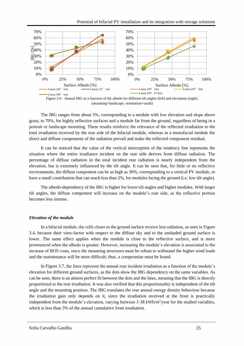
Potential of bifacial PV installation and its integration with storage solutions
Sofia Carvalho Ganilha 25
The IBG ranges from about 5%, corresponding to a module with low elevation and slope above
grass, to 70%, for highly reflective surfaces and a module far from the ground, regardless of being in a
portrait or landscape mounting. These results reinforce the relevance of the reflected irradiation to the
total irradiation received by the rear side of the bifacial module, whereas in a monofacial module the
direct and diffuse components of the radiation prevail and make the reflected component residual.
It can be noticed that the value of the vertical interception of the tendency line represents the
situation where the entire irradiance incident on the rear side derives from diffuse radiation. The
percentage of diffuse radiation in the total incident rear radiation is nearly independent from the
elevation, but is extremely influenced by the tilt angle. It can be seen that, for little or no reflective
environments, the diffuse component can be as high as 30%, corresponding to a vertical PV module, or
have a small contribution that can reach less than 2%, for modules facing the ground (i.e. low tilt angle).
The albedo-dependency of the IBG is higher for lower tilt angles and higher modules. With larger
tilt angles, the diffuse component will increase on the module’s rear side, as the reflective portion
becomes less intense.
Elevation of the module
In a bifacial module, the cells closer to the ground surface receive less radiation, as seen in Figure
3.4, because their view-factor with respect to the diffuse sky and to the unshaded ground surface is
lower. The same effect applies when the module is close to the reflective surface, and is more
pronounced when the albedo is greater. However, increasing the module’s elevation is associated to the
increase of BOS costs, since the mounting structures must be robust to withstand the higher wind loads
and the maintenance will be more difficult; thus, a compromise must be found.
In Figure 3.7, the lines represent the annual rear incident irradiation as a function of the module’s
elevation for different ground surfaces, as the dots show the IBG dependency on the same variables. As
can be seen, there is an almost perfect fit between the dots and the lines, meaning that the IBG is directly
proportional to the rear irradiation. It was also verified that this proportionality is independent of the tilt
angle and the mounting position. The IBG translates the rear annual energy density behaviour because
the irradiation gain only depends on it, since the irradiation received at the front is practically
independent from the module’s elevation, varying between 3-38 kWh/m2/year for the studied variables,
which is less than 3% of the annual cumulative front irradiation.
0%
10%
20%
30%
40%
50%
60%
70%
0% 25% 50% 75% 100%
IBG
[%
]
Surface Albedo [%]Linear (45º 1m) Linear (15º 1m)
Linear (90º 1m)
0%
10%
20%
30%
40%
50%
60%
70%
0% 25% 50% 75% 100%
Surface Albedo [%]Linear (45º 1m) Linear (45º 2m)
Linear (45º 0.15m)
Figure 3.6 - Annual IBG as a function of the albedo for different tilt angles (left) and elevations (right).
(mounting=landscape; orientation=south)

CHAPTER 3. Irradiance bifacial model
Sofia Carvalho Ganilha 26
As the module’s elevation increases, the self-shadowing of the rear side decreases and the diffuse
radiation intercepted intensifies, the mix of the two effects results in the full benefit of the reflected
radiation from the underlying surface and the growth of rear annual cumulative energy density. These
effects are more accentuated for landscape modules closer to the ground surface, because the view-
factor between the upper cells and the unshaded part of the ground is less than for portrait modules, as
well as the diffuse radiation collected.
Above an elevation of 0.6 meters, for 45º inclined portrait modules, the rear irradiation saturates,
as well as the total irradiation. The saturation behaviour is explained by the fact that the regions of the
underlying reflective surface farther away from the bifacial solar module have less contribution to the
irradiation intercepted by the rear surface of the module. This saturation can be reached for lower
elevations if the tilt angle is very pronounced, since the diffuse radiation that can be captured is
maximum and more relevant than the reflected component. If the PV module has a low tilt angle, the
effects of self-shading are more noticeable and the elevation from which the rear irradiation saturates is
higher. The mounting position also impacts the elevation when the saturation is reached, nearly
duplicating it in the case of landscape modules, as explained in the previous paragraph.
3.2.3. Optimization of the configuration for a PV stand
The IBG of a single bifacial module and a bifacial PV stand are not comparable, because the
reflected irradiance captured by the rear side of the modules depends on the ground shading that is
influenced by the area utilization and PV packing density, i.e. the distance between and within rows.
Therefore, it is important to estimate these effects on the bifacial gains of a PV power plant.
0%
10%
20%
30%
40%
50%
60%
70%
0
200
400
600
800
1000
1200
1400
0.0 0.5 1.0 1.5 2.0
IBG
[%
]
Rea
r an
nu
al c
um
ula
tiv
e en
erg
y d
ensi
ty
[kW
h/m
²]
Elevation [m]Asphalt White Painted Concrete Grass Grey Tiles White Gravel
Figure 3.7 – Dependency of the annual rear cumulative irradiation (lines) and the IBG (dots) on the elevation and ground
surface (tilt=45º; mounting=landscape; orientation=south).
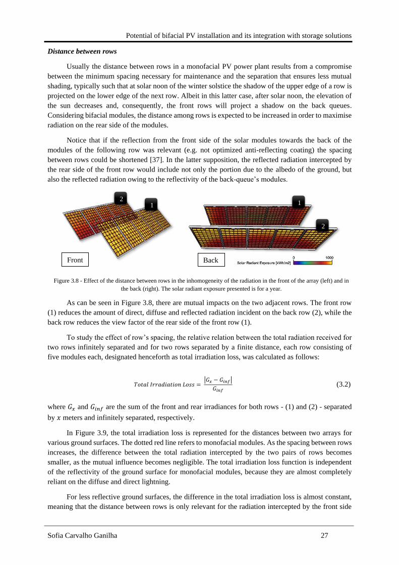
Potential of bifacial PV installation and its integration with storage solutions
Sofia Carvalho Ganilha 27
Distance between rows
Usually the distance between rows in a monofacial PV power plant results from a compromise
between the minimum spacing necessary for maintenance and the separation that ensures less mutual
shading, typically such that at solar noon of the winter solstice the shadow of the upper edge of a row is
projected on the lower edge of the next row. Albeit in this latter case, after solar noon, the elevation of
the sun decreases and, consequently, the front rows will project a shadow on the back queues.
Considering bifacial modules, the distance among rows is expected to be increased in order to maximise
radiation on the rear side of the modules.
Notice that if the reflection from the front side of the solar modules towards the back of the
modules of the following row was relevant (e.g. not optimized anti-reflecting coating) the spacing
between rows could be shortened [37]. In the latter supposition, the reflected radiation intercepted by
the rear side of the front row would include not only the portion due to the albedo of the ground, but
also the reflected radiation owing to the reflectivity of the back-queue’s modules.
As can be seen in Figure 3.8, there are mutual impacts on the two adjacent rows. The front row
(1) reduces the amount of direct, diffuse and reflected radiation incident on the back row (2), while the
back row reduces the view factor of the rear side of the front row (1).
To study the effect of row’s spacing, the relative relation between the total radiation received for
two rows infinitely separated and for two rows separated by a finite distance, each row consisting of
five modules each, designated henceforth as total irradiation loss, was calculated as follows:
where 𝐺𝑥 and 𝐺𝑖𝑛𝑓 are the sum of the front and rear irradiances for both rows - (1) and (2) - separated
by 𝑥 meters and infinitely separated, respectively.
In Figure 3.9, the total irradiation loss is represented for the distances between two arrays for
various ground surfaces. The dotted red line refers to monofacial modules. As the spacing between rows
increases, the difference between the total radiation intercepted by the two pairs of rows becomes
smaller, as the mutual influence becomes negligible. The total irradiation loss function is independent
of the reflectivity of the ground surface for monofacial modules, because they are almost completely
reliant on the diffuse and direct lightning.
For less reflective ground surfaces, the difference in the total irradiation loss is almost constant,
meaning that the distance between rows is only relevant for the radiation intercepted by the front side
𝑇𝑜𝑡𝑎𝑙 𝐼𝑟𝑟𝑎𝑑𝑖𝑎𝑡𝑖𝑜𝑛 𝐿𝑜𝑠𝑠 = |𝐺𝑥 − 𝐺𝑖𝑛𝑓|
𝐺𝑖𝑛𝑓 (3.2)
1 2
2
1
Front Back
Figure 3.8 - Effect of the distance between rows in the inhomogeneity of the radiation in the front of the array (left) and in
the back (right). The solar radiant exposure presented is for a year.
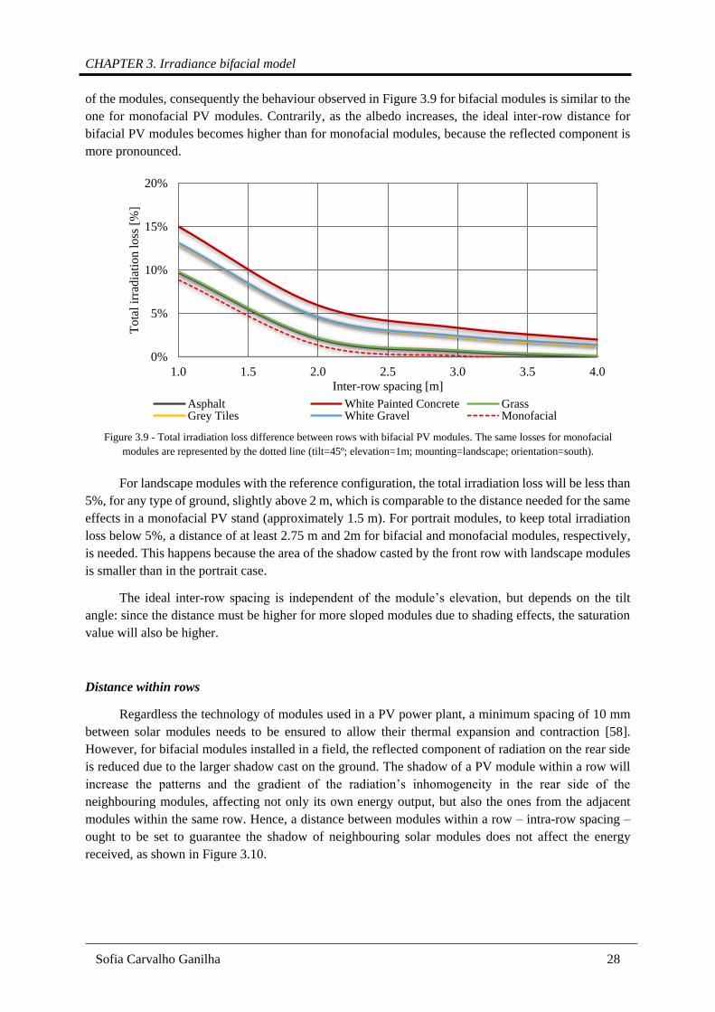
CHAPTER 3. Irradiance bifacial model
Sofia Carvalho Ganilha 28
of the modules, consequently the behaviour observed in Figure 3.9 for bifacial modules is similar to the
one for monofacial PV modules. Contrarily, as the albedo increases, the ideal inter-row distance for
bifacial PV modules becomes higher than for monofacial modules, because the reflected component is
more pronounced.
For landscape modules with the reference configuration, the total irradiation loss will be less than
5%, for any type of ground, slightly above 2 m, which is comparable to the distance needed for the same
effects in a monofacial PV stand (approximately 1.5 m). For portrait modules, to keep total irradiation
loss below 5%, a distance of at least 2.75 m and 2m for bifacial and monofacial modules, respectively,
is needed. This happens because the area of the shadow casted by the front row with landscape modules
is smaller than in the portrait case.
The ideal inter-row spacing is independent of the module’s elevation, but depends on the tilt
angle: since the distance must be higher for more sloped modules due to shading effects, the saturation
value will also be higher.
Distance within rows
Regardless the technology of modules used in a PV power plant, a minimum spacing of 10 mm
between solar modules needs to be ensured to allow their thermal expansion and contraction [58].
However, for bifacial modules installed in a field, the reflected component of radiation on the rear side
is reduced due to the larger shadow cast on the ground. The shadow of a PV module within a row will
increase the patterns and the gradient of the radiation’s inhomogeneity in the rear side of the
neighbouring modules, affecting not only its own energy output, but also the ones from the adjacent
modules within the same row. Hence, a distance between modules within a row – intra-row spacing –
ought to be set to guarantee the shadow of neighbouring solar modules does not affect the energy
received, as shown in Figure 3.10.
0%
5%
10%
15%
20%
1.0 1.5 2.0 2.5 3.0 3.5 4.0
To
tal
irra
dia
tion
lo
ss [
%]
Inter-row spacing [m]
Asphalt White Painted Concrete GrassGrey Tiles White Gravel Monofacial
Figure 3.9 - Total irradiation loss difference between rows with bifacial PV modules. The same losses for monofacial
modules are represented by the dotted line (tilt=45º; elevation=1m; mounting=landscape; orientation=south).

Potential of bifacial PV installation and its integration with storage solutions
Sofia Carvalho Ganilha 29
To study the effect of module’s spacing, the IBG for each module within a row (consisting of
eight modules) was calculated, which is possible because the front irradiance is assumed to be equal for
all modules and, consequently, the IBG difference between the modules at the middle and extreme of
the row translates the difference between the rear irradiance collected by the two. Results are shown in
Figure 3.11.
As expected, duo to the shadows casted by neighbouring modules that reduce the reflected
radiation, the modules on the extremities of a row receive more radiant energy than those in the middle.
Thus, the modules at the edge of the field have a higher IBG. This effect is more accentuated if the
distance between adjacent modules is small. The mutual shading is negligible for module’s spacing
above 1 m. It can also be seen that the IBG difference is higher for surfaces with a higher albedo, given
its dependency of optimal rear conditions for reflection.
The acceptable intra-row distance for modules with the longer edge parallel to the surface is
slightly less than the one for portrait PV modules, varying between 0.5 and 1 m, since the casted shadow
is also smaller and the distance between the highest cells and the reflective surface is lower.
Figure 3.12 shows that the shading effects affect more the modules closer to the ground, because
of the larger view factors between the shaded region and the solar cells. For vertical modules, as they
rely more on the diffuse component than on the reflected radiation, the intra-row distance is constant.
However, as the tilt angle decreases, the IBG difference between the extreme and middle modules
increases, because the view-factor relatively to the shadowed ground increases, thus the intra-row
Figure 3.10 - Effect of the distance between the modules within rows in the inhomogeneity of the rear radiation. The solar
radiant exposure presented is for a year.
0%
5%
10%
15%
20%
0.0 0.5 1.0 1.5 2.0IBG
dif
fere
nce
bet
wee
n t
he
edge
and
mid
dle
mod
ule
s [%
]
Intra or within row spacing [m]
Asphalt White Painted Concrete Grass Grey Tiles White Gravel
Figure 3.11 - IBG difference within a row for different spacing between modules, considering the reference module (tilt=45º;
elevation=1m; orientation=south).

CHAPTER 3. Irradiance bifacial model
Sofia Carvalho Ganilha 30
spacing must be bigger. Nevertheless, the differences of IBG between the modules in the edge and
middle of the PV array are small enough to be attributed to the simulation accuracy.
It ought to be noticed that the optimum distance between modules and rows is not only determined
by the irradiance optimization but also other relevant factors such as the land available or the increasing
cost of BOS with installation area.
0%
5%
10%
15%
20%
25%
30%
0.0 0.5 1.0 1.5 2.0
IBG
dif
fere
nce
bet
wee
n t
he
edg
e an
d m
idd
le m
od
ule
s [%
]
Intra-row spacing [m]
15º 1m 45º 1m 90º 1m
0%
5%
10%
15%
20%
25%
30%
0.0 0.5 1.0 1.5 2.0
IBG
dif
fere
nce
bet
wee
n t
he
edg
e an
d m
idd
le m
od
ule
s [%
]
Intra-row spacing [m]
45º 0.15m 45º 1m 45º 2m
Figure 3.12 - Module's spacing dependency on elevation (left) and tilt angle (right) considering the reference model
(ground=white gravel; orientation=south).
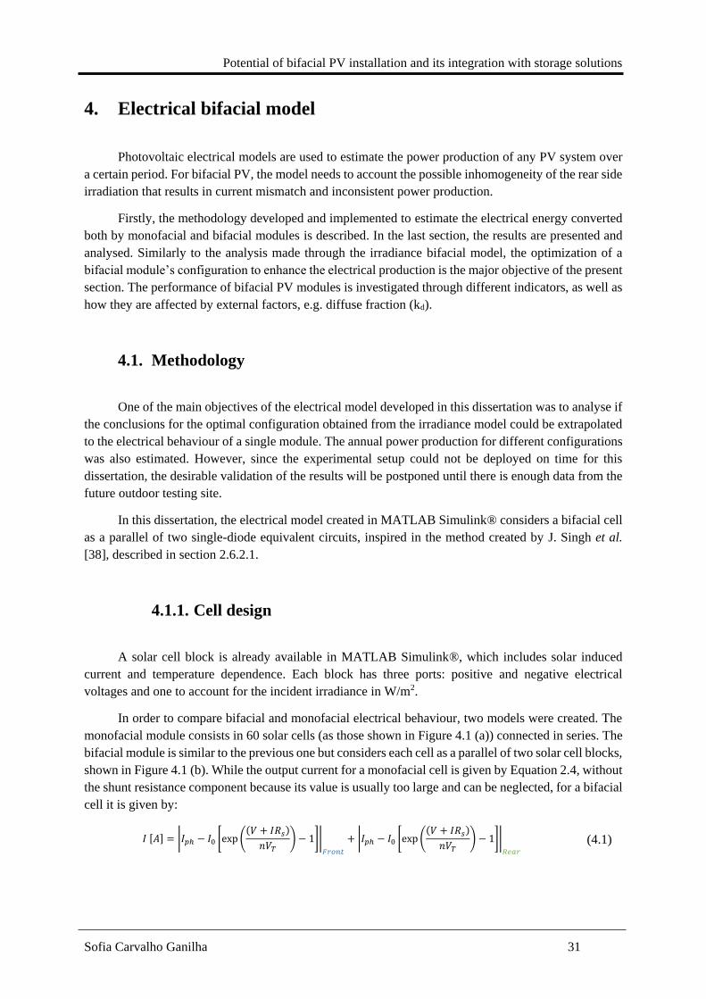
Potential of bifacial PV installation and its integration with storage solutions
Sofia Carvalho Ganilha 31
4. Electrical bifacial model
Photovoltaic electrical models are used to estimate the power production of any PV system over
a certain period. For bifacial PV, the model needs to account the possible inhomogeneity of the rear side
irradiation that results in current mismatch and inconsistent power production.
Firstly, the methodology developed and implemented to estimate the electrical energy converted
both by monofacial and bifacial modules is described. In the last section, the results are presented and
analysed. Similarly to the analysis made through the irradiance bifacial model, the optimization of a
bifacial module’s configuration to enhance the electrical production is the major objective of the present
section. The performance of bifacial PV modules is investigated through different indicators, as well as
how they are affected by external factors, e.g. diffuse fraction (kd).
4.1. Methodology
One of the main objectives of the electrical model developed in this dissertation was to analyse if
the conclusions for the optimal configuration obtained from the irradiance model could be extrapolated
to the electrical behaviour of a single module. The annual power production for different configurations
was also estimated. However, since the experimental setup could not be deployed on time for this
dissertation, the desirable validation of the results will be postponed until there is enough data from the
future outdoor testing site.
In this dissertation, the electrical model created in MATLAB Simulink® considers a bifacial cell
as a parallel of two single-diode equivalent circuits, inspired in the method created by J. Singh et al.
[38], described in section 2.6.2.1.
4.1.1. Cell design
A solar cell block is already available in MATLAB Simulink®, which includes solar induced
current and temperature dependence. Each block has three ports: positive and negative electrical
voltages and one to account for the incident irradiance in W/m2.
In order to compare bifacial and monofacial electrical behaviour, two models were created. The
monofacial module consists in 60 solar cells (as those shown in Figure 4.1 (a)) connected in series. The
bifacial module is similar to the previous one but considers each cell as a parallel of two solar cell blocks,
shown in Figure 4.1 (b). While the output current for a monofacial cell is given by Equation 2.4, without
the shunt resistance component because its value is usually too large and can be neglected, for a bifacial
cell it is given by:
𝐼 [𝐴] = |𝐼𝑝ℎ − 𝐼0 [exp ((𝑉 + 𝐼𝑅𝑠)
𝑛𝑉𝑇) − 1]|
𝐹𝑟𝑜𝑛𝑡
+ |𝐼𝑝ℎ − 𝐼0 [exp ((𝑉 + 𝐼𝑅𝑠)
𝑛𝑉𝑇) − 1]|
𝑅𝑒𝑎𝑟
(4.1)
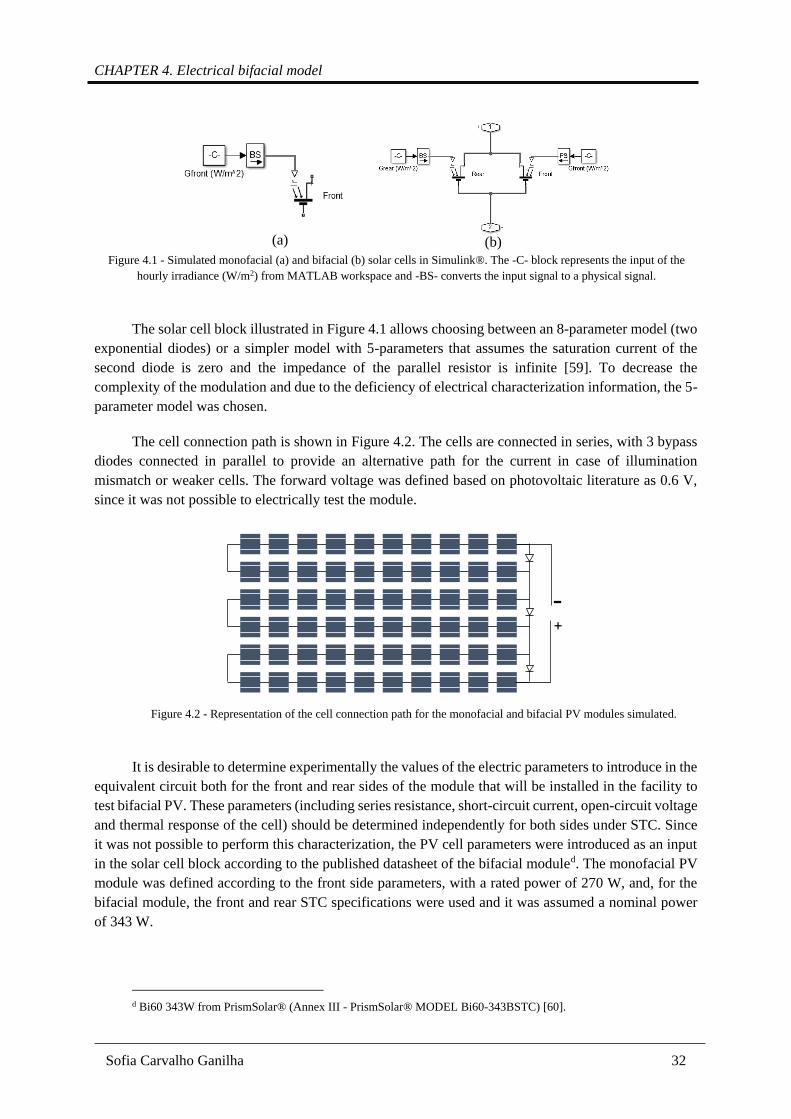
CHAPTER 4. Electrical bifacial model
Sofia Carvalho Ganilha 32
The solar cell block illustrated in Figure 4.1 allows choosing between an 8-parameter model (two
exponential diodes) or a simpler model with 5-parameters that assumes the saturation current of the
second diode is zero and the impedance of the parallel resistor is infinite [59]. To decrease the
complexity of the modulation and due to the deficiency of electrical characterization information, the 5-
parameter model was chosen.
The cell connection path is shown in Figure 4.2. The cells are connected in series, with 3 bypass
diodes connected in parallel to provide an alternative path for the current in case of illumination
mismatch or weaker cells. The forward voltage was defined based on photovoltaic literature as 0.6 V,
since it was not possible to electrically test the module.
It is desirable to determine experimentally the values of the electric parameters to introduce in the
equivalent circuit both for the front and rear sides of the module that will be installed in the facility to
test bifacial PV. These parameters (including series resistance, short-circuit current, open-circuit voltage
and thermal response of the cell) should be determined independently for both sides under STC. Since
it was not possible to perform this characterization, the PV cell parameters were introduced as an input
in the solar cell block according to the published datasheet of the bifacial moduled. The monofacial PV
module was defined according to the front side parameters, with a rated power of 270 W, and, for the
bifacial module, the front and rear STC specifications were used and it was assumed a nominal power
of 343 W.
d Bi60 343W from PrismSolar® (Annex III - PrismSolar® MODEL Bi60-343BSTC) [60].
(a)
(b)
Figure 4.1 - Simulated monofacial (a) and bifacial (b) solar cells in Simulink®. The -C- block represents the input of the
hourly irradiance (W/m2) from MATLAB workspace and -BS- converts the input signal to a physical signal.
Figure 4.2 - Representation of the cell connection path for the monofacial and bifacial PV modules simulated.

Potential of bifacial PV installation and its integration with storage solutions
Sofia Carvalho Ganilha 33
Table 4.1 summarizes the electrical characteristics for the solar cell block parameterization.
While Isc and Voc were extracted from the module’s datasheet (STC), the series resistance was calculated
according to 4.2 [61].
𝑅𝑠 [Ω] =
𝛼𝑆𝑇𝐶 ln (1 −𝐼𝑚𝑝𝑝,𝑆𝑇𝐶
𝐼𝑠𝑐,𝑆𝑇𝐶) + 𝑉𝑜𝑐,𝑆𝑇𝐶 − 𝑉𝑚𝑝𝑝,𝑆𝑇𝐶
𝐼𝑚𝑝𝑝,𝑆𝑇𝐶 (4.2)
where 𝛼𝑆𝑇𝐶 is the thermal voltage timing completion factor for STC [61]. The value of the remaining
parameters was left as default. TIPH1, TXIS1 and TRS1 are coefficients for the temperature dependence
upon the solar-induced current, the diode’s saturation current and the series resistance, respectively [59].
Table 4.1 - Electrical parameters for the front and rear sides of the solar cell introduced in Simulink®.
Parameter Front Side Cell Rear Side Cell
Short-circuit current (A) 8.98 7.96
Open-circuit voltage (V) 0.65 0.64
Quality factor (diode
emission coefficient) 1.5 1.5
Series resistance (𝛀) 0.072 0.079
TIPH1 (1/K) 0 0
TXIS1 3 3
TRS1 0 0
4.1.2. Thermal model
One of the inputs of the solar cell block is the cell’s temperature. Although the temperature
variation of each cell within the module is highly dependent on the speed and direction of the wind and
on the incident radiation, which may not be homogenous throughout the module, this variable is assumed
to be constant for the entire PV module. Despite the simplicity of the assumption made in order to
decrease the complexity of the electrical modulation, its limitations are kept in mind.
Following the discussion in section 2.6.2.2., the temperature of monofacial modules was
calculated using Equation 2.11 and the thermal behaviour of bifacial PV modules was predicted by the
model developed by Sandia National Laboratories and given by Equation 2.12, in which the wind speed
and ambient temperature from TMY were used. For a glass/cell/glass module type mounted on an open
rack, 𝑎 = −3.47 and 𝑏 = −0.0594 [45].
Once the experimental setup is deployed, the temperature may be assessed by sensors or IR
thermography of operating modules.

CHAPTER 4. Electrical bifacial model
Sofia Carvalho Ganilha 34
4.1.3. Model dynamics
For each cell, the hourly rear and front incident irradiances were estimated in Rhinoceros® based
on the mean value of 16 radiation sensors distributed uniformly throughout the PV cell. These
predictions are processed in MATLAB®, as well as the wind velocity and ambient temperature of
Lisbon’s TMY. Then, the temperature of the module is estimated based on the equations presented in
section 4.1.2. and using the imported data. These values are directly introduced in the corresponding
ports of the solar cell blocks in the Simulink® electrical model.
Figure 4.3 presents the Simulink model where the solar module is connected to a variable resistor.
The resistance varies linearly according to an input ramp with a slope of 1 ohm. An amperemeter and a
voltmeter are used to determine the photo-generated current and the voltage at the terminals of the
resistor, respectively. The product of both variables is registered in a power array and sent to
MATLAB’s workspace. This power array consists in the power delivered by the module according to
the value of the load’s resistance, during a simulation time of 100 seconds.
a A MATLAB® routine was developed to determine the Maximum Power Point (MPP) of
operation for the solar module. A flowchart of the MPP tracker technique implemented is presented in
Figure 4.4.
After the routine is complete, the MPP of operation for all hours of the year is recorded.
Figure 4.3 - Simulink electrical model of a PV module.
Figure 4.4 - Flowchart of the algorithm implemented in MATLAB to find the MPP.
Potential of bifacial PV installation and its integration with storage solutions
Sofia Carvalho Ganilha 35
4.1.4. Performance indicators
To assess the performance of bifaciality and compare bifacial PV systems with those that use
monofacial PV modules, different indicators can be used. The comparison must cover economical,
efficiency and energy generation factors.
Bifacial Gain (BG)
BG has already been defined in Equation 2.2. The main focus of this work is the assessment of
the energy boost attributed to bifacial PV, which is why most of the comparisons will be made using a
BG calculated only according to the absolute energy yield, henceforth designated by Energy Bifacial
Gain (EBG). This indicator is adequate to compare the energy converted per unit area. Thus, it will be
considered that a 270 W monofacial PV module approximately occupies the same effective area than a
343 W bifacial PV module. EBG is adequate to express an idealistic perspective of the PV market, where
the kWh produced is more valuable than the Wp installed.
Though, to take into account the economical point of view, some investigators defend that BG
should be calculated using the energy generated divided by the nominal peak power - specific yield
(Wh/Wp) -, which allows the evaluation of the system also in terms of technology costs. This perspective
translates the current paradigm of the PV market.
In order to allow a comprehensive comparison, both indicators will be used when appropriate.
Performance Ratio (PR)
PR is an indicator commonly used to evaluate the energy efficiency and reliability of a PV system
and compare it with that of other PV plants, independently of the incident solar irradiation, location and
time period. It is defined as the ratio of the measured to the theoretically expected energy output of the
system, and numerically it is given by:
𝑃𝑅 =∫ 𝑃𝑀𝑃𝑃 𝑑𝑡
𝑃𝑛𝑜𝑚 ×∫ 𝐼𝑟𝑟𝑎𝑑𝑖𝑎𝑛𝑐𝑒 𝑑𝑡
𝑅𝑒𝑓𝑒𝑟𝑒𝑛𝑐𝑒 𝐼𝑟𝑟𝑎𝑑𝑖𝑎𝑛𝑐𝑒
(4.3)
whereas 𝑃𝑀𝑃𝑃 is the power output at the MPP and 𝑃𝑛𝑜𝑚 is the rated nominal power of the PV module. The
reference irradiance was considered 1000 W/m2 (front) plus 300 W/m2 (rear) for bifacial modules, and
only 1000 W/m2 for monofacial modules under STC, as specified in the datasheet. For bifaciality
analysis, the total irradiance over 1 year was used, taking into account data from both front and rear
sides.
An efficient PV system usually achieves an average PR that lies between 80% and 90%
throughout the year [2].
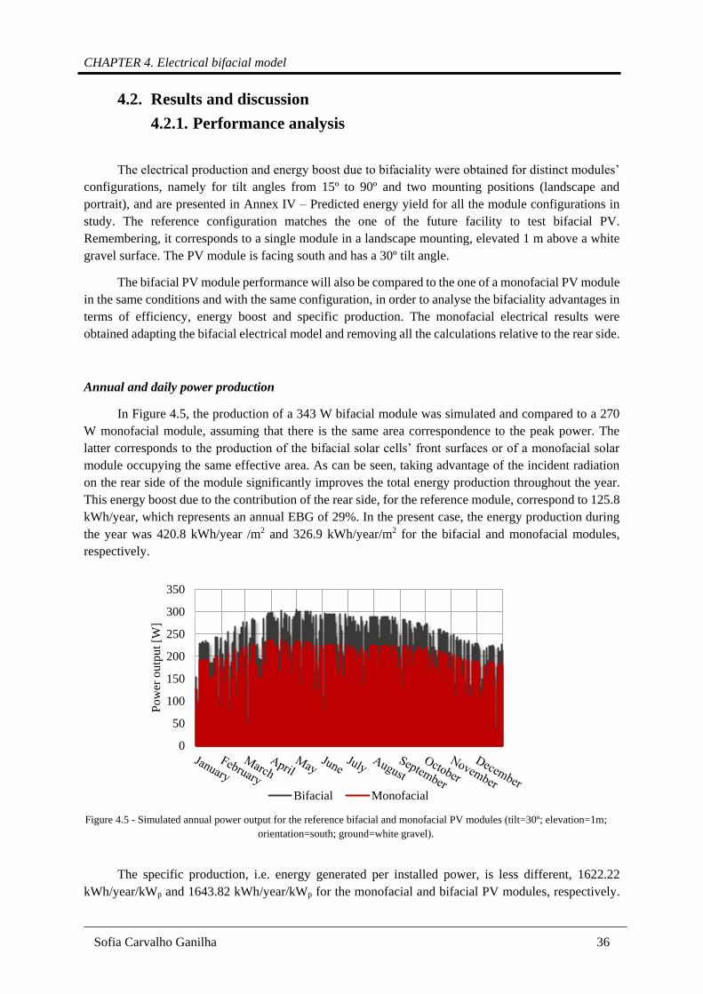
CHAPTER 4. Electrical bifacial model
Sofia Carvalho Ganilha 36
4.2. Results and discussion
4.2.1. Performance analysis
The electrical production and energy boost due to bifaciality were obtained for distinct modules’
configurations, namely for tilt angles from 15º to 90º and two mounting positions (landscape and
portrait), and are presented in Annex IV – Predicted energy yield for all the module configurations in
study. The reference configuration matches the one of the future facility to test bifacial PV.
Remembering, it corresponds to a single module in a landscape mounting, elevated 1 m above a white
gravel surface. The PV module is facing south and has a 30º tilt angle.
The bifacial PV module performance will also be compared to the one of a monofacial PV module
in the same conditions and with the same configuration, in order to analyse the bifaciality advantages in
terms of efficiency, energy boost and specific production. The monofacial electrical results were
obtained adapting the bifacial electrical model and removing all the calculations relative to the rear side.
Annual and daily power production
In Figure 4.5, the production of a 343 W bifacial module was simulated and compared to a 270
W monofacial module, assuming that there is the same area correspondence to the peak power. The
latter corresponds to the production of the bifacial solar cells’ front surfaces or of a monofacial solar
module occupying the same effective area. As can be seen, taking advantage of the incident radiation
on the rear side of the module significantly improves the total energy production throughout the year.
This energy boost due to the contribution of the rear side, for the reference module, correspond to 125.8
kWh/year, which represents an annual EBG of 29%. In the present case, the energy production during
the year was 420.8 kWh/year /m2 and 326.9 kWh/year/m2 for the bifacial and monofacial modules,
respectively.
The specific production, i.e. energy generated per installed power, is less different, 1622.22
kWh/year/kWp and 1643.82 kWh/year/kWp for the monofacial and bifacial PV modules, respectively.
0
50
100
150
200
250
300
350
Pow
er o
utp
ut
[W]
Bifacial Monofacial
Figure 4.5 - Simulated annual power output for the reference bifacial and monofacial PV modules (tilt=30º; elevation=1m;
orientation=south; ground=white gravel).

Potential of bifacial PV installation and its integration with storage solutions
Sofia Carvalho Ganilha 37
Although the lack of standards for bifacial PV modules affects these values, a tenuous advantage due to
bifaciality and associated to the system costs can be confirmed, since most of intrinsic costs relative to
the module (e.g. price of the module) are proportional to Wp.
The daily power production of the reference module and EBG for a typical day (17/August) is
represented in Figure 4.6. The peak power in a clear sky day PV production curve is achieved by both
monofacial and bifacial modules at solar noon. However, it is when the diffuse fraction is higher that
we observe a major EBG, because the contribution of the irradiance on the back of the module is higher
comparatively to the front side. Thus, the maximum EBG is not achieved when the energy production
is larger.
The main contribution of the rear side of the PV module relatively to the front surface happens
mostly during sunrise and sunset and cloudy days. At these latitudes (Lisbon) between equinoxes (during
the spring and summer months), the sun’s azimuth on the sunset and sunrise is closer to North, meaning
that there is direct irradiation striking directly the rear side of the PV module.
If the EBG is represented through the year and in function of the hour, the effects described
previously can be visualized, resulting in Figure 4.7 and Figure 4.8, respectively.
In Figure 4.7, the hourly EBG for the entire year of analysis is represented by the red dots. As can
be seen, the EBG is always positive, which means bifacial PV modules convert more energy per square
meter comparatively to a monofacial module throughout the year. The majority of the divergent EBG,
represented by the overlapped black dots, occurs between March and September, during which happens
the equinoxes. Also, higher EBG are verified in the spring and summer, not only because of the
contribution of direct irradiance, but also because the reflected component increases.
0%
10%
20%
30%
40%
50%
60%
0
50
100
150
200
250
300
350
EB
G [
%]
Pow
er o
utp
ut
[W]
Bifacial Monofacial EBG
Figure 4.6 - Daily variation of the EBG and predicted power production for the reference module on 17/August (tilt=30º;
elevation=1m; orientation=south; ground=white gravel).
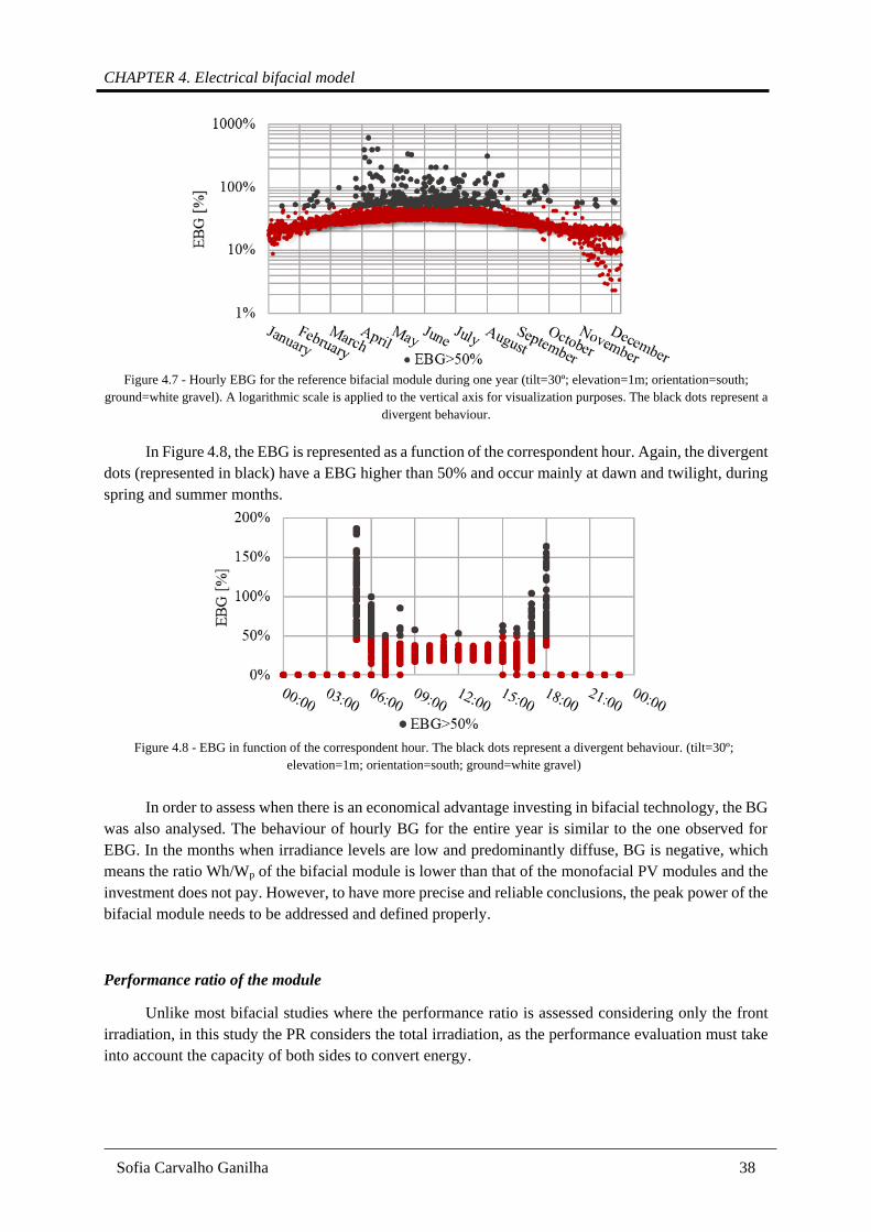
CHAPTER 4. Electrical bifacial model
Sofia Carvalho Ganilha 38
In Figure 4.8, the EBG is represented as a function of the correspondent hour. Again, the divergent
dots (represented in black) have a EBG higher than 50% and occur mainly at dawn and twilight, during
spring and summer months.
In order to assess when there is an economical advantage investing in bifacial technology, the BG
was also analysed. The behaviour of hourly BG for the entire year is similar to the one observed for
EBG. In the months when irradiance levels are low and predominantly diffuse, BG is negative, which
means the ratio Wh/Wp of the bifacial module is lower than that of the monofacial PV modules and the
investment does not pay. However, to have more precise and reliable conclusions, the peak power of the
bifacial module needs to be addressed and defined properly.
Performance ratio of the module
Unlike most bifacial studies where the performance ratio is assessed considering only the front
irradiation, in this study the PR considers the total irradiation, as the performance evaluation must take
into account the capacity of both sides to convert energy.
a
a
Figure 4.7 - Hourly EBG for the reference bifacial module during one year (tilt=30º; elevation=1m; orientation=south;
ground=white gravel). A logarithmic scale is applied to the vertical axis for visualization purposes. The black dots represent a
divergent behaviour.
Figure 4.8 - EBG in function of the correspondent hour. The black dots represent a divergent behaviour. (tilt=30º;
elevation=1m; orientation=south; ground=white gravel)

Potential of bifacial PV installation and its integration with storage solutions
Sofia Carvalho Ganilha 39
Figure 4.9 shows the monthly average PR for the reference bifacial and monofacial PV modules.
The PR is stable, with a slightly seasonal variation. In the summer months when the direct component
of irradiance is predominant, both PV modules perform less efficiently comparatively to the rest of the
year.
The annual average PR for the monofacial is 85.8%, while for the bifacial is 83.8%, which means
an annual difference of 2% is found between the two technologies; but monofacial is consistently higher.
Tilt angle optimization and its influence on the power production
Figure 4.10 presents the simulation results for the annual production of a bifacial and monofacial
PV modules as a function of the tilt angle as well as the energy and irradiance bifacial gains.
Once again, it can be noticed that the angle that maximizes the annual energy production, thus the
optimum value for the tilt of the bifacial module, does not match the angle that maximizes the EBG.
Through a polynomial regression, it was determined the optimum tilt angle as approximately 39º, which
is slightly less than the angle that maximizes the total irradiation intercepted by the bifacial module
(41º).
0%
20%
40%
60%
80%
100%
PR
[%
]
Bifacial Monofacial
Figure 4.9 - Monthly evaluation of the PR for a single monofacial and bifacial modules with the reference configuration
(tilt=30º; elevation=1m; orientation=south; ground=white gravel).
Figure 4.10 - Annual energy production estimation for monofacial and bifacial modules with the reference configuration
(elevation=1m; orientation=south; ground=white gravel). In the right vertical axis is represented the IBG and EBG for the
bifacial PV module.
0%
10%
20%
30%
40%
50%
-
100
200
300
400
500
600
15 30 45 60 75 90
IBG
an
d E
BG
[%
]
Ann
ual
en
erg
y p
rodu
ctio
n
[kW
h]
Tilt [°]
Bifacial Monofacial EBG IBG

CHAPTER 4. Electrical bifacial model
Sofia Carvalho Ganilha 40
The EBG is maximum in the case of 90º, because at a higher tilt angle, the rear side of the module
is more exposed to diffuse and reflected irradiation and, simultaneously, the front side production
decreases due to less direct radiation intercepted (non-optimal conditions), consequently the ratio
between the rear and front side production increases. As the tilt angle approximates the ideal conditions,
the front side production has a larger influence, since more direct radiation is intercepted, and the EBG
decreases. Lastly, when the tilt angle is lower than the optimum value, the ratio rear/front irradiances
and EBG increases, since the photo-generated current of the front side in non-optimal conditions also
decreases.
There is a high correspondence between EBG and IBG, suggesting a proportionality relation that
will be analysed in the subsequent sections (4.2.2.).
Influence of the mounting position on the power production
The inhomogeneity of the radiation at the back of the bifacial PV module will result in a photo-
generated current mismatch that negatively affects its electrical output. The radiation gradient in the rear
side is strongly influenced by the distance between the reflector (unshaded part of the ground) and the
cell, the tilt angle and the ground surface’s reflectivity. Mounting the modules in a landscape or portrait
mode provides a way to control how the irregular incident irradiation impacts a series of cells actuated
by a bypass diode, which euphemizes the effects of irradiation inhomogeneity.
To understand the influence of the mounting position in the electrical output, the annual energy
generated and the EBG for the reference module are shown in Table 4.2. The landscape modules allow
a more efficient utilization of the bypass diodes. However, the annual advantage is negligible for
landscape modules (additional 0.1%) and, since the annual front irradiation is almost independent of the
mounting mode, it indicates that the amplitude and gradient of the front irradiation far exceeds the rear
surface effects.
Table 4.2 - Annual energy generation and EBG for the reference module in a portrait and landscape mounting position
(tilt=30º; elevation=1m; orientation=south; ground=white gravel).
Mounting
Position
Energy
Generated
(kWh/year)
EBG (%)
Landscape 563.8 28.7
Portrait 563.5 28.6
Module’s mounting is expected to be irrelevant only when a single module or a stand with a
proper inter-row and intra-row distances is being considered, because, in these cases, the casted shadow
by each PV module does not influence the radiation received by the rear sides of the neighbouring
bifacial PV modules.
Besides, in real conditions where the area utilization factor is determined not only by efficiency
reasons, but also economical and logistical ones, landscape mounting is associated to a minor self-
shadowing phenomenon. Choosing this configuration to increase the energy conversion is associated
with other advantages, such as the minor inter and within rows distances comparatively to portrait
modules; thus, all these considerations must be taken into account.

Potential of bifacial PV installation and its integration with storage solutions
Sofia Carvalho Ganilha 41
Influence of the module’s orientation on the power production
The orientation of PV modules is a powerful tool to regulate and passively control the energy
generation. For instance, installing a bifacial PV module in a vertical position facing east/west may be
more suitable to balance the power production and consumption.
Before exploring a self-consumption installation implementing this configuration (in terms of tilt
angle and orientation), in chapter 5, it is desirable to analyse the daily and annual power production of
vertical east and west modules and compare it with the production of the reference module facing south.
The visual comparison between the daily power production curves of vertical bifacial modules
orientated towards east and west and a south-facing 30º tilted bifacial module is shown in Figure 4.11.
For the east and west-facing bifacial modules, two power peaks occur in the early and later hours
of the day, between 7h-10h and 14h-16h, respectively, because in this time period the total incident
irradiation is almost completely direct irradiation, since the PV modules are directly facing the sun.
However, at solar noon, the sun is approximately in the same plane as the modules’ surfaces and most
of the collected irradiation is diffuse and reflected by the ground, which can be visualized in the figure
by the midday valley.
In spite of its potential for peak shifting, the power estimated at solar noon for bifacial vertical
modules facing east/west is in an annual average 32% lower than the same module with optimum tilt
and orientation, which cumulatively represents a reduction of the annual output.
It is important to reinforce that the rear and front sides of the bifacial PV module are electrically
different and, therefore, the power output will be different for a module facing east or west. The surface
facing east receives annually more irradiation than the other one, which numerically translates into
1 675.5 kWh/year and 1 349.9 kWh/year, respectivelye, because according to the TMY, the radiation in
the morning hours is tendentially greater than it is after solar noon. Besides, the morning peak of the
east-facing PV module (i.e. most efficient side turned to east) is, in an annual average, 6% higher than
the one turned to west (i.e. most efficient side turned to west) and, in opposition, the afternoon peak of
the west-facing PV module is, in an annual average, 7% higher than the west-facing PV module.
e This asymmetry may be dramatically increased or decreased in the urban environment, when the shading from other
buildings is considered.
0
50
100
150
200
250
300
350
Pow
er o
utp
ut
[W]
90º East 30º South 90º West
Figure 4.11 - Daily generated power curve for three bifacial modules with specific orientations and tilt angles on 17/August
(elevation=1m; ground=white gravel).

CHAPTER 4. Electrical bifacial model
Sofia Carvalho Ganilha 42
For the whole year, the absolute energy yield is 496.19 kWh for the east-facing PV module and
489.04 kWh for west-facing module, which corresponds to a 1% difference, which is not significant in
terms of production. However, in terms of suitability to the load diagram, the orientation can be used as
a tool to supply energy the consumer in the morning or evening peak.
4.2.2. Externalities that affect the bifacial gain
Relation between IBG and EBG
Figure 4.10 suggested that there is proportionality between the IBG and the EBG, which means
the energy generation boost increases linearly with the incident radiation boost of a bifacial module.
This relation is confirmed in Figure 4.12. This result has a big impact in the early stage of the
construction of a bifacial PV installation, because it allows to be more time-efficient when determining
the configuration of the modules that allows to take the biggest advantage of bifaciality, since the
optimization can be based on the incident irradiation, avoiding the calculations related to the energy
output, which must include the electric and thermal models of the modules.
It must be noticed that the configuration that increases bifacial gains does not guarantee the
maximization neither of the intercepted irradiance nor of the energy produced.
In Figure 4.12, it is possible to observe the “outliers” due to the direct received irradiation at the
back of the module at dawn and at twilight in spring and summer months. Although there are higher
EBG and IBG than those represented, they were omitted from the figure to facilitate its readability.
Relation between diffuse fraction (kd) and EBG
The performance of a bifacial module strongly depends on the diffuse fraction (kd), i.e. the ratio
between the diffuse and the total irradiance.
To study the effect of the total irradiance components (direct and diffuse) on the energy boost of
bifacial modules relatively to monofacial PV modules, the EBG is plotted against the diffuse fraction
a
R² = 0.994
0%
15%
30%
45%
60%
75%
90%
105%
120%
135%
150%
0% 20% 40% 60% 80% 100% 120% 140% 160% 180% 200%
EB
G [
%]
IBG [%]
Figure 4.12 - Representation of the EBG as a function of the IBG for the bifacial reference module (tilt=30º;
elevation=1m; orientation=south; ground=white gravel).

Potential of bifacial PV installation and its integration with storage solutions
Sofia Carvalho Ganilha 43
(kd is calculated hourly according to the TMY of Lisbon) and shown in Figure 4.13. Once again, the
divergent dots that have an EBG higher than 50% are represented in black.
The results show that there is a slight increase of EBG with the diffuse fraction, as clearly shown
by the best fit line (in black) shown. This result was to be expected, as a high diffuse content is related
to a significant increase of the incident irradiation on the rear side of the module and, simultaneously, a
decrease on the front surface due to the lower direct irradiance comparatively to a clear-sky day. Thus,
the photo-generated current from the front side decreases as the bifacial energy boost increases due to
the rear side photo-generated current. This is the same reason why EBG is relatively lower around solar
noon. The impacts of having a high diffuse fraction occur predominantly in cloudy days, early in the
morning or late in the afternoon.
Nevertheless, these results also show that there are many other factors affecting EBG, such as the
module temperature, determined by the ambient temperature and the PV technology itself, which
introduce a high level of variability. For this reason, there is no clear pattern in Figure 4.13.
EBG = 0.061*kd + 0.258
R² = 0.0333
0%15%30%45%60%75%90%
105%120%135%150%
0% 20% 40% 60% 80% 100%
EB
G [
%]
kd [%]
EBG>50%
Figure 4.13 - Representation of the EBG as a function of the kd for the bifacial reference module. The black dots represent a
divergent behaviour. (tilt=30º; elevation=1m; orientation=south; ground=white gravel).

CHAPTER 5. Integration of bifacial PV with storage solutions
Sofia Carvalho Ganilha 44
5. Integration of bifacial PV with storage solutions
Finally, in the present chapter, the methodology to determine which configuration and modules
should be implemented in order to optimize the storage capacity of a residential self-consumption
solution is described. The results are presented later in this chapter.
In Portugal, the law decree n. º 153/2014 published in October 2014, defines the legal framework
for Units of Production for Self-Consumption (UPAC). Self-consumption is a convenient solution for a
distributed production regime. It consists in RES electricity’s production, mainly intended to be
consumed on-site of use. It is possible for an UPAC to be connected to the electrical grid, so the electrical
energy produced can either be injected to the grid and sold in the market or stored for later consumption
when it is required [62].
The possibility of self-consumption enables the PV systems’ wider deployment for residential
consumers and contributes to the integration of RES onto the electricity grid, possibly mitigating some
of its technical challenges, such as power ramps, frequency regulation, voltage amplitude fluctuations
and grid energy losses [63].
5.1. Methodology
5.1.1. Self-consumption performance indicators
As it was already seen in discussed section 2.6.3., bifacial PV brings new possibilities for self-
consumption at a residential scale, not only because bifaciality is more area-effective, but also because
it may allow a better fit of the electricity generation to the daily load consumption profile, which opens
a feasible possibility to decrease the storage capacity and its the associated costs.
For yearly simulations, the main performance indicator is the total volume of self-consumption,
which is commonly expressed as Self-Consumption Rate (SCR) or as Self-Sufficiency Rate (SSR) [64].
In numerical terms, SCR is the fraction of PV generation directly self-consumed (without passing
through the battery) or from the storage unit, defined by Equation 5.1.
𝑆𝐶𝑅 = 𝐸𝑠𝑡𝑜𝑟𝑎𝑔𝑒 𝑑𝑖𝑠𝑐ℎ𝑎𝑟𝑔𝑒 + 𝐸𝑃𝑉 𝑑𝑖𝑟𝑒𝑐𝑡𝑙𝑦 𝑠𝑒𝑙𝑓−𝑐𝑜𝑛𝑠𝑢𝑚𝑒𝑑
𝑁𝑒𝑡 𝑔𝑒𝑛𝑒𝑟𝑎𝑡𝑖𝑜𝑛 (5.1)
The SSR assesses the percentage of the energy demand that is fulfilled by on-site PV production,
presented in Equation 5.2.
𝑆𝑆𝑅 = 𝐸𝑠𝑡𝑜𝑟𝑎𝑔𝑒 𝑑𝑖𝑠𝑐ℎ𝑎𝑟𝑔𝑒 + 𝐸𝑃𝑉 𝑑𝑖𝑟𝑒𝑐𝑡𝑙𝑦 𝑠𝑒𝑙𝑓−𝑐𝑜𝑛𝑠𝑢𝑚𝑒𝑑
𝑁𝑒𝑡 𝑙𝑜𝑎𝑑 (5.2)
Both indicators will be determined considering two different perspectives. The first one
normalizes by the area the energy converted by the monofacial and bifacial modules, which privileges
the price per m2, and the second one normalizes it by the PV nominal peak power, which is associated
to the current price/Wp mentality.
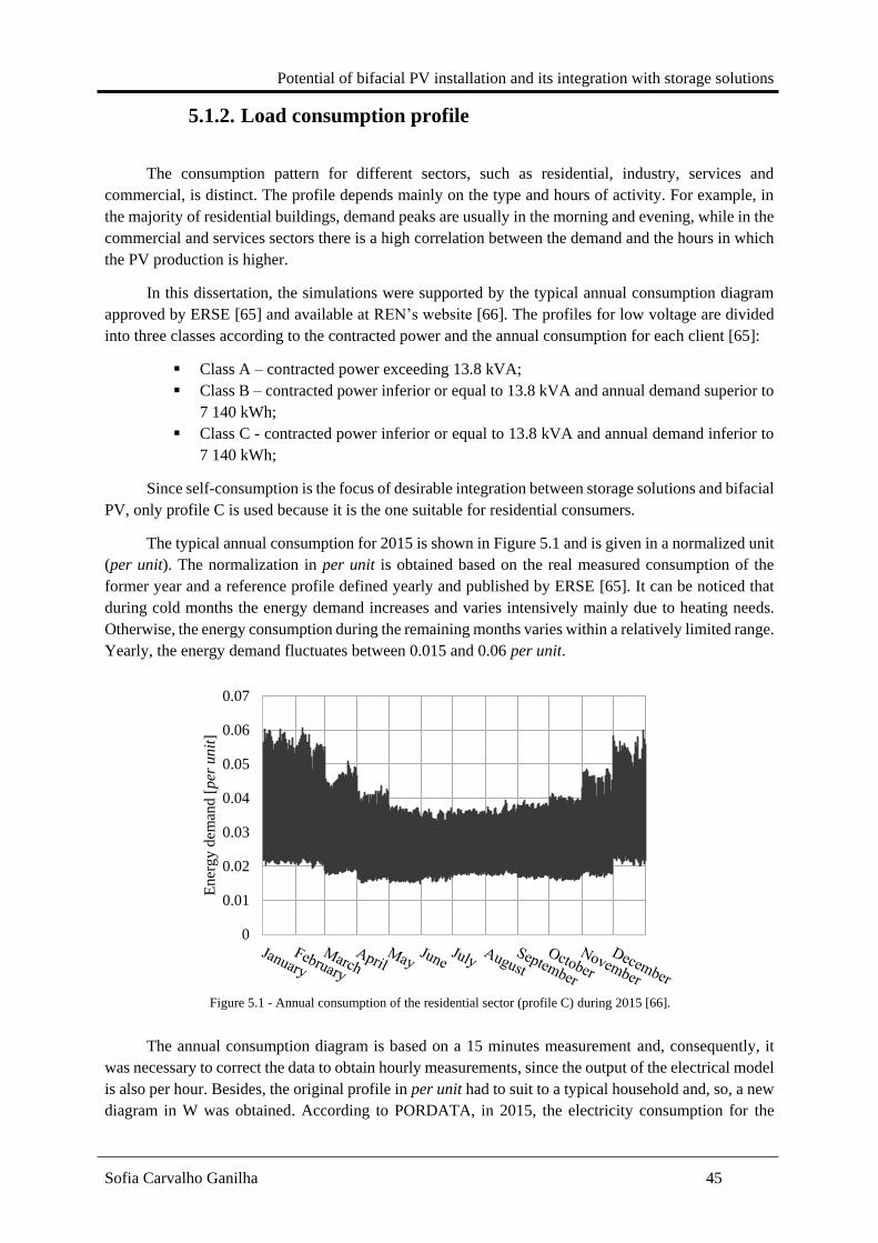
Potential of bifacial PV installation and its integration with storage solutions
Sofia Carvalho Ganilha 45
5.1.2. Load consumption profile
The consumption pattern for different sectors, such as residential, industry, services and
commercial, is distinct. The profile depends mainly on the type and hours of activity. For example, in
the majority of residential buildings, demand peaks are usually in the morning and evening, while in the
commercial and services sectors there is a high correlation between the demand and the hours in which
the PV production is higher.
In this dissertation, the simulations were supported by the typical annual consumption diagram
approved by ERSE [65] and available at REN’s website [66]. The profiles for low voltage are divided
into three classes according to the contracted power and the annual consumption for each client [65]:
▪ Class A – contracted power exceeding 13.8 kVA;
▪ Class B – contracted power inferior or equal to 13.8 kVA and annual demand superior to
7 140 kWh;
▪ Class C - contracted power inferior or equal to 13.8 kVA and annual demand inferior to
7 140 kWh;
Since self-consumption is the focus of desirable integration between storage solutions and bifacial
PV, only profile C is used because it is the one suitable for residential consumers.
The typical annual consumption for 2015 is shown in Figure 5.1 and is given in a normalized unit
(per unit). The normalization in per unit is obtained based on the real measured consumption of the
former year and a reference profile defined yearly and published by ERSE [65]. It can be noticed that
during cold months the energy demand increases and varies intensively mainly due to heating needs.
Otherwise, the energy consumption during the remaining months varies within a relatively limited range.
Yearly, the energy demand fluctuates between 0.015 and 0.06 per unit.
The annual consumption diagram is based on a 15 minutes measurement and, consequently, it
was necessary to correct the data to obtain hourly measurements, since the output of the electrical model
is also per hour. Besides, the original profile in per unit had to suit to a typical household and, so, a new
diagram in W was obtained. According to PORDATA, in 2015, the electricity consumption for the
0
0.01
0.02
0.03
0.04
0.05
0.06
0.07
En
erg
y d
eman
d [
per
un
it]
Figure 5.1 - Annual consumption of the residential sector (profile C) during 2015 [66].

CHAPTER 5. Integration of bifacial PV with storage solutions
Sofia Carvalho Ganilha 46
residential sector per capita was 1 156.1 kWh, and the average size of private households was 2.5 people
[67]. Thus, for simulation purposes, it was considered a residence with an annual demand of 2 890.2
kWh.
5.1.3. Configuration of the PV installation
One of the major challenges to self-consumption based on a PV system in a residential scale is
the time lag between peaks in the daily load profile and in the optimized power production diagram. To
enlarge the potential of self-consumption for household units it is possible to modify the configuration
of the PV modules, such as their orientation and tilt angle.
Using vertical bifacial PV modules facing east/west can partially solve the problem, because it
can shift the production peaks from noon to the morning and evening, when more energy is needed in a
typical household. In addition, if monofacial or bifacial modules facing south are included in the system,
the generation profile can be softened.
To study which configuration or combination of the PV modules is more suitable to ensure a good
correlation between the load profile and the PV generation diagram, the hourly production estimated in
the electrical model for four modules’ configurations was used, as presented in Table 5.1. It is important
to notice that a bifacial module facing east means that it has its most efficient side turned to that direction,
and the same happens with the bifacial PV module turned to west.
Table 5.1 - Configurations of the PV modules tested to integrate in a PV system with storage.
Number Module Type Tilt Angle Orientation
1 Monofacial 30º South
2 Bifacial 30º South
3 Bifacial 90º East
4 Bifacial 90º West
The study considered that the PV modules are above white gravel.
5.1.4. Self-consumption installation
A storage system may be used to increase the SCR and the SSR, in a self-consumption scenario.
Besides the battery storage system, the PV installation also includes an inverter, the PV modules and
the charge controller, as shown in Figure 5.2.
The charge controller sets the strategy to determine the energy fluxes’ direction. Firstly, the
energy generated by the PV modules is used to fulfil the load demand. If there is surplus energy, it is
used to charge the battery, if needed, and the remaining is sold to the grid. When the PV production is
lower than the consumption, the energy gap will be assured by the battery, if charged, and the remaining
bought from the grid.
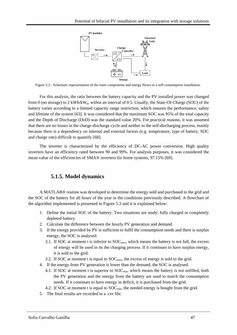
Potential of bifacial PV installation and its integration with storage solutions
Sofia Carvalho Ganilha 47
For this analysis, the ratio between the battery capacity and the PV installed power was changed
from 0 (no storage) to 2 kWh/kWp, within an interval of 0.5. Usually, the State-Of-Charge (SOC) of the
battery varies according to a limited capacity range restriction, which ensures the performance, safety
and lifetime of the system [63]. It was considered that the maximum SOC was 95% of the total capacity
and the Depth of Discharge (DoD) was the standard value 20%. For practical reasons, it was assumed
that there are no losses in the charge-discharge cycle and neither in the self-discharging process, mainly
because there is a dependency on internal and external factors (e.g. temperature, type of battery, SOC
and charge rate) difficult to quantify [68].
The inverter is characterized by the efficiency of DC-AC power conversion. High quality
inverters have an efficiency rated between 90 and 99%. For analysis purposes, it was considered the
mean value of the efficiencies of SMA® inverters for home systems, 97.15% [69].
5.1.5. Model dynamics
A MATLAB® routine was developed to determine the energy sold and purchased to the grid and
the SOC of the battery for all hours of the year in the conditions previously described. A flowchart of
the algorithm implemented is presented in Figure 5.3 and it is explained below:
1. Define the initial SOC of the battery. Two situations are study: fully charged or completely
depleted battery.
2. Calculate the difference between the hourly PV generation and demand.
3. If the energy provided by PV is sufficient to fulfil the consumption needs and there is surplus
energy, the SOC is analysed.
3.1. If SOC at moment t is inferior to SOCmax, which means the battery is not full, the excess
of energy will be used in its the charging process. If it continues to have surplus energy,
it is sold to the grid.
3.2. If SOC at moment t is equal to SOCmax, the excess of energy is sold to the grid.
4. If the energy from PV generation is lower than the demand, the SOC is analysed.
4.1. If SOC at moment t is superior to SOCmin, which means the battery is not unfilled, both
the PV generation and the energy from the battery are used to match the consumption
needs. If it continues to have energy in deficit, it is purchased from the grid.
4.2. If SOC at moment t is equal to SOCmin, the needed energy is bought from the grid.
5. The final results are recorded in a .csv file.
Figure 5.2 - Schematic representation of the main components and energy fluxes in a self-consumption installation.

CHAPTER 5. Integration of bifacial PV with storage solutions
Sofia Carvalho Ganilha 48
5.2. Results and discussion
Vertically mounted bifacial PV systems are thought to have a large potential to be implemented
in a diverse range of applications. Taking advantage of bifaciality in order to upgrade self-consumption
solutions is one of the promising applications. It is desirable to have a timely coincidence between the
PV generation and the power consumption profiles for economic (locally consumed electricity is more
valued than surplus electricity sold to the grid) and technical reasons (lower interaction with the grid
reduces losses) and it is expected that vertical bifacial PV modules may contribute to a better matching
between the two daily diagrams.
In this chapter, the energy consumption, generation and storage are analysed from the point of
view of a residential consumer with a self-consumption system that integrates one of four possible PV
module configurations and technologies.
5.2.1. PV generation
The PV generation system is a component of a self-consumption installation. It not only directly
provides energy to respond to the load, but also enables the charge process of the battery’s bank and an
economic income from the sale of the surplus solar electricity.
There are three main factors affecting the generation diagram and energy yield of the PV system:
its size (Wp or m2 installed, both are analysed), orientation/inclination and location.
Figure 5.3 - Flowchart of the algorithm implemented in MATLAB to model the dynamics of a self-consumption with storage
system.

Potential of bifacial PV installation and its integration with storage solutions
Sofia Carvalho Ganilha 49
The PV system is considered to be installed in Lisbon, so the meteorological conditions will
equally affect all the PV modules, independently of their orientations or installed capacities. Three
orientations will be analysed: single monofacial and bifacial PV modules orientated towards south, and
single bifacial PV modules facing east and west.
In a “power produced by m2” perspective, for each one of the previous configurations, the number
of PV modules will vary between 1 and 6 modules, i.e. an effective area that ranges between 1.34 and
8.04 m2, and therefore the installed capacity varies between 0.27 and 1.62 kWp or between 0.34 and 2.06
kWp for the monofacial and bifacial PV systems, respectively. However, it will also be considered a
different perspective: “power produced by Wp installed”. In this case, the PV technologies considered
(monofacial and bifacial) are forced to have the same nominal peak power, which varies between 0.34
and 2.06 kWp, without having in consideration the area installed.
To illustrate the annual PV generation variability, the original estimation of the average monthly
power production calculated through the electrical model for a 270 W monofacial module and a 343 W
bifacial module are shown in Figure 5.4, highlighting the orientations in study.
The solar power is higher when the incident direct irradiance is more intense, i.e. during the
summer months, independently of the technology or orientation of the modules. However, the
monofacial production is more constant during the year. This comparison is only valid if the interest is
in the energy produced per square meter, i.e. the annual energy produced is normalized by the effective
area of the modules. In this case, there is a clear advantage in using a bifacial solar module with an
optimal tilt angle and orientation, because the energy produced is higher than in the remain cases for the
same installation area.
The comparison presented in the previous paragraph is an unrealistic vision, because currently
the PV power installed is more valued than the PV production area. However, to enable bifacial’s
worldwide spreading, the PV market paradigm must be changed from cost/Wp to cost/m2.
To ensure a fair comparison between the modules also through an economical point of view, the
PV data must be normalized by the peak power, i.e. the annual power production is divided by the
nominal peak power of the modules, since it is only possible to compare the energy yield and the cost
Figure 5.4 - Simulated monthly mean power output normalized by the area for the modules’ types and configurations
analysed for a self-consumption solution. The mean values were calculated only for the solar hours.
0
50
100
150
200
250
Mo
nth
ly M
ean
Pow
er O
utp
ut
[W]
30º South Monofacial 30º South Bifacial 90º East Bifacial 90º West Bifacial

CHAPTER 5. Integration of bifacial PV with storage solutions
Sofia Carvalho Ganilha 50
of different systems if their installed capacity is equal. Therefore, the specific and absolute energy yield
for the PV configurations analysed are presented in Table 5.2.
Table 5.2 – Specific and absolute energy yield for the modules’ types and configurations analysed for the self-consumption
solution.
Module Type Tilt Angle Peak Power
(W) Orientation
Specific Yield
(kWh/kWp)
Absolute Energy
Yield (kWh/m2)
Monofacial 30º 270 South 1.62 326.86
Bifacial 30º 343 South 1.64 420.77
Bifacial 90º 343 East 1.45 370.29
Bifacial 90º 343 West 1.43 364.96
As expected, bifacial modules facing south improve the energy yield of the system for the entire
year and, consequently, the EBG and BG. However, the energy boost for the same production area, i.e.
EBG, is higher than the improvements in terms of kWh/kWp, i.e. BG.
Even if the orientation and tilt are not optimal for a bifacial solar module, the energy produced
per unit area is bigger than in the monofacial case. However, in economic terms, the specific yield of
the vertical modules is not comparable to south-facing modules. For this reason, the only advantages of
using bifacial modules facing east or west may be an improved area-production efficiency and a better
match between the production and consumption’s daily profiles, as will be seen latter.
The daily specific yield for the four configurations studied is shown in Figure 5.5. The red line
represents the annual average specific yield for each hour.
The daily behaviour of (a) and (b) is very similar, which means apparently there is no economical
advantage investing in a bifacial solar system. Comparatively to the remaining orientations, the specific
yield is higher and the peaks of power production occur around 12:00. During summer, the peak
increases and can reach 0.89 kW/kWp.
However, in an energy converted per m2 perspective, i.e. analysing the energy produced within
the same area, albeit the format of the curves remains the same (the daily power density for the four
configurations studied is shown in Annex V – Daily power density PV curve for the module’s
configurations considered for the self-consumption solution), the power peak in (b) is considerably
higher than that in (a). The average peak power density is 155.58 W/m2 for the south-facing bifacial PV
and only 123.25 W/m2 for the monofacial PV module.
On the other hand, the power curves (c) and (d) have two humps, one early in the morning (7h-
10h) and the other in the afternoon (14h-16h). These peaks correspond to the moments when one of the
bifacial module’s surfaces is receiving direct radiation from the sun. (c) corresponds to the vertical
bifacial module whose more efficient side is facing east and so, associated to the fact that the east surface
receives annually more irradiation, the morning peak is higher than the one in the afternoon. For (c), the
mean morning peak is 0.46 kW/kWp or 116.55 W/m2 and the afternoon peak is 0.35 kW/kWp or 90.14
W/m2. Relatively to (d), its peaks are more similar, because the more efficient side is facing west, which
is the side that receives less irradiation, thus increasing the afternoon’s production comparatively to (c),
and, simultaneously, the combination of the less efficient cell surface with the side that receives more
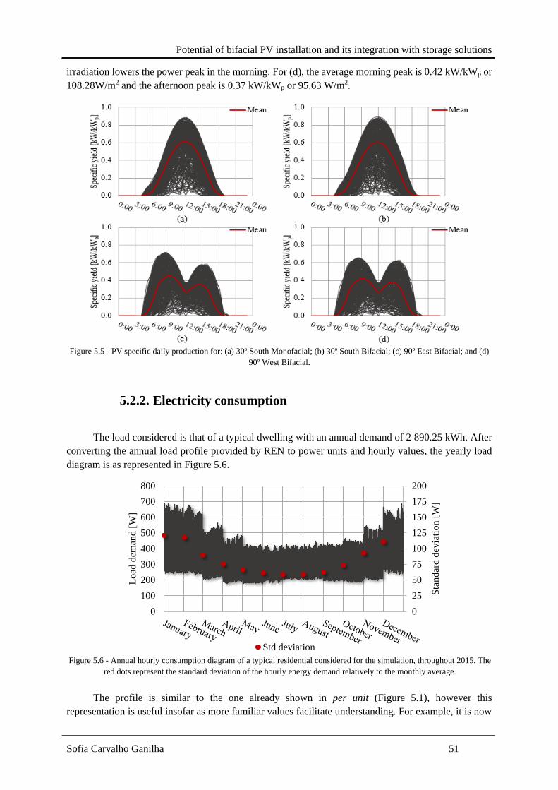
Potential of bifacial PV installation and its integration with storage solutions
Sofia Carvalho Ganilha 51
irradiation lowers the power peak in the morning. For (d), the average morning peak is 0.42 kW/kWp or
108.28W/m2 and the afternoon peak is 0.37 kW/kWp or 95.63 W/m2.
5.2.2. Electricity consumption
The load considered is that of a typical dwelling with an annual demand of 2 890.25 kWh. After
converting the annual load profile provided by REN to power units and hourly values, the yearly load
diagram is as represented in Figure 5.6.
The profile is similar to the one already shown in per unit (Figure 5.1), however this
representation is useful insofar as more familiar values facilitate understanding. For example, it is now
a
Figure 5.5 - PV specific daily production for: (a) 30º South Monofacial; (b) 30º South Bifacial; (c) 90º East Bifacial; and (d)
90º West Bifacial.
0
25
50
75
100
125
150
175
200
0
100
200
300
400
500
600
700
800
Sta
ndar
d d
evia
tion [
W]
Lo
ad d
eman
d [
W]
Std deviation
Figure 5.6 - Annual hourly consumption diagram of a typical residential considered for the simulation, throughout 2015. The
red dots represent the standard deviation of the hourly energy demand relatively to the monthly average.

CHAPTER 5. Integration of bifacial PV with storage solutions
Sofia Carvalho Ganilha 52
obvious that the hourly demand in cold months varies between approximately 200 and 700 W, while in
the rest of the year it ranges between 200 and 450 W. The standard deviation for each month is also
represented. It shows that the variability of the hourly demand relatively to the mean value in January,
February, November and December is higher than for the rest of the year. Thus, the demand range is
wider during the cold months, not only because of the heating systems usage but also because people
tend to stay indoors. Considering an annual scale, the demand peak is 688 W.
The consumption profile can also be represented according to the daily hour, in order to
understand the habits of the inhabitants with regard to electricity needs. In Figure 5.7 the individual
hourly demand is represented based on the hour of the day, as well as the annual, summer and winter
mean load diagrams.
There are mainly two peaks of electricity demand in the daily load diagram. The first one happens
during 10:00 to 13:00 period and the second one from 18:00 to 21:00. These peaks occur during time
periods of high activity, generally associated to lunch and dinner time. There is also a high variability
of energy demand during all day, except from 3:00 to 6:00, which is correlated to the activity and
inactivity time of the inhabitants, respectively.
It is possible to observe a decrease of the energy needs during summer and an increase throughout
winter relatively to the mean electricity demand, which is in accordance with the reasons already
presented (heating necessities and longer periods of human occupancy).
5.2.3. Self-consumption system dynamics
The self-consumption system (PV-Battery-Load-Grid) was simulated for different battery
capacities and PV systems, in terms of installed power, technology and orientation. The dynamic of the
system consists in the energy flows’ determination, in time steps of one hour:
▪ The amount of PV generated energy (including the fraction that is directly consumed, fed
into the grid or used to charge the battery);
▪ The quantity of self-consumed energy that comes from the battery;
0
100
200
300
400
500
600
700
800
Lo
ad d
eman
d [
W]
Annual mean Summer mean Winter mean
Figure 5.7 - Daily hourly load diagram for the residence of the analysis.

Potential of bifacial PV installation and its integration with storage solutions
Sofia Carvalho Ganilha 53
▪ The total purchased energy from the grid.
To better understand the dynamic of a self-consumption system, the energy fluxes will be
illustrated in the following figures, assuming that the capacity of the storage unit is fixed at 1 kWh/kWp.
For now, there is no interest in comparing the performance of the self-consumption system among the
different PV systems’ configurations neither the storage capacities, which will be the focus of section
5.2.4.
Once again, two different perspectives will be analysed: the first one considers that the energy
should be normalized and, consequently, charged by the unit area. The second one is the current PV
market reality that privileges the Wp thinking and, therefore, the energy converted is normalized by the
nominal peak capacity. For the first perspective, the dynamic of a self-consumption system with two
solar modules, as exposed in section 5.2.1., independently of the technology employed, will be analysed.
As for the second perspective, it will be considered that the bifacial and monofacial modules have the
same peak power, 343 W. Two solar modules will be used, in order to surpass the annual peak demand
and, simultaneously, minimize the surplus energy.
For a PV system constituted by two 30º bifacial solar modules south-facing, the fluxes of energy
to satisfy the load demand are represented in Figure 5.8. This system is able to completely satisfy the
consumption needs from 8:00 to 16:00. Besides, during this period, 918.7 Wh are injected to the grid
and 514.5 Wh are used to charge the battery’s bank. The presence of a storage system extends the self-
consumption period until 19:00. On 17th August, approximately 45.3% of the load demand was provided
directly by the PV system and 7.2% by the battery, which means that self-consumption was assured by
the solar energy generation in more than 50%.
For the entire year, approximately 64% of the energy needed was supplied from the grid and only
36% was provided by the PV system.
If the intention is to analyse and compare the use of a bifacial solar module with a monofacial one
with the same installed peak, the energy produced by two 30º monofacial solar modules south-facing
must be normalized by the PV peak power. In this case, the installed power of the monofacial PV module
was that of the bifacial PV module and, consequently, the profiles in analysis overlap to the ones
represented in Figure 5.8, reason why the representation of the energy fluxes is omitted. The annual
amount of energy provided by the monofacial PV system+storage and by the grid to the load is similar
a
Figure 5.8 - Self-consumption dynamic for a system with two 30º bifacial solar modules facing south with 343 W each
(17/August).
0
100
200
300
400
500
600
700
Pow
er [
W]
PV generated Battery Discharge From Grid PV Directly Consumed Load

CHAPTER 5. Integration of bifacial PV with storage solutions
Sofia Carvalho Ganilha 54
to the bifacial case, approximately 35% and 65%, respectively. Although the difference is very small,
there is still a slight advantage for the bifacial technology.
Bifacial solar modules are more area-effective in this type of applications, because to produce as
much as a bifacial PV module, it would require larger monofacial PV modules. However, if the area
available is limited, the distances between bifacial PV modules to ensure that there isn’t mutual shading
may not be respected and the power production will be compromised.
If one considers the case where within the same area the power reason between monofacial and
bifacial solar modules is 270 W:343 W, the energy fluxes are represented in Figure 5.9 for the
monofacial PV module. As can be seen, the surplus energy during the period in which the PV generation
is superior to the load energy needs is inferior, approximately 600.1 Wh (202.5Wh are used to charge
the battery and 397.6 Wh are injected to the grid). Therefore, bifaciality is beneficial, as it increases the
self-sufficiency period and the possibility to generate more income thanks to the energy sold to the grid,
occupying the same area as a less powerful monofacial module. For the entire year, approximately 70%
of the energy needed was injected from the grid and only 30% was provided by the PV system+storage.
For the same area, the PV power installed is different for monofacial and bifacial modules (Figure
5.8 and Figure 5.9), therefore the storage capacity also changes because it is thinking in a kWh/kWp
perspective. Thus, for the bifacial cases considered, the battery can store and provide more energy when
required. This is the main reason why the portion correspondent to “Battery Discharge” in Figure 5.8 is
bigger than the one in Figure 5.9.
For a PV system constituted by two vertical bifacial solar modules facing east, the fluxes of energy
to satisfy the load demand are represented in Figure 5.10. In this case, the two humps in the production
diagram are immediately before consumption’s peaks, and therefore excess energy in those periods can
be used to charge the batteries in order to be used in the peaks, increasing self-consumption and self-
sufficiency rates. On 17th August, almost half (48.5%) of the load demand was provided directly by the
PV system and 8.8% by the battery, which means that, for this day in particular, there is a significant
benefit for the vertical bifacial module.
Figure 5.9 - Self-consumption dynamic for a system with two 30º monofacial solar modules facing South with 270 W each
(17/August).
0
100
200
300
400
500
600
700
Pow
er [
W]
PV generated Battery Discharge From Grid PV Directly Consumed Load
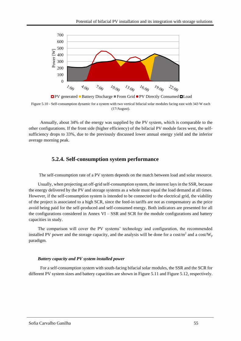
Potential of bifacial PV installation and its integration with storage solutions
Sofia Carvalho Ganilha 55
Annually, about 34% of the energy was supplied by the PV system, which is comparable to the
other configurations. If the front side (higher efficiency) of the bifacial PV module faces west, the self-
sufficiency drops to 33%, due to the previously discussed lower annual energy yield and the inferior
average morning peak.
5.2.4. Self-consumption system performance
The self-consumption rate of a PV system depends on the match between load and solar resource.
Usually, when projecting an off-grid self-consumption system, the interest lays in the SSR, because
the energy delivered by the PV and storage systems as a whole must equal the load demand at all times.
However, if the self-consumption system is intended to be connected to the electrical grid, the viability
of the project is associated to a high SCR, since the feed-in tariffs are not as compensatory as the price
avoid being paid for the self-produced and self-consumed energy. Both indicators are presented for all
the configurations considered in Annex VI – SSR and SCR for the module configurations and battery
capacities in study.
The comparison will cover the PV systems’ technology and configuration, the recommended
installed PV power and the storage capacity, and the analysis will be done for a cost/m2 and a cost/Wp
paradigm.
Battery capacity and PV system installed power
For a self-consumption system with south-facing bifacial solar modules, the SSR and the SCR for
different PV system sizes and battery capacities are shown in Figure 5.11 and Figure 5.12, respectively.
Figure 5.10 - Self-consumption dynamic for a system with two vertical bifacial solar modules facing east with 343 W each
(17/August).
0
100
200
300
400
500
600
700
Pow
er [
W]
PV generated Battery Discharge From Grid PV Directly Consumed Load
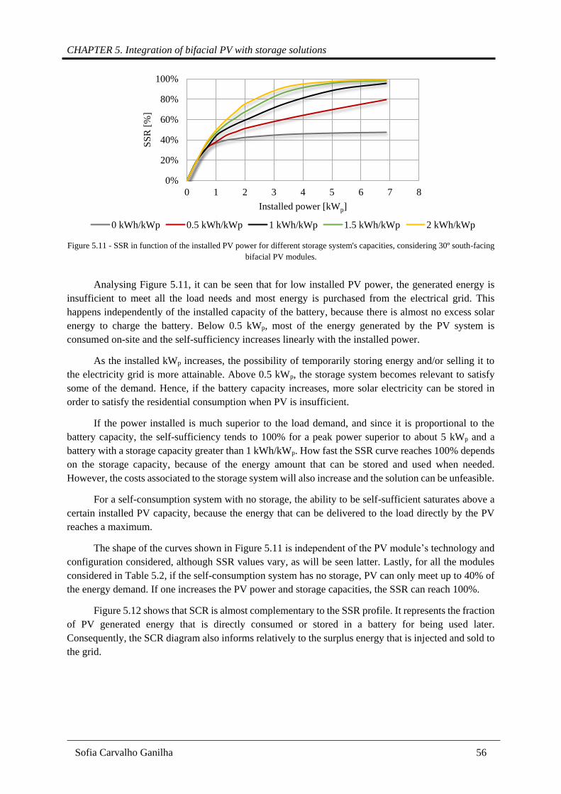
CHAPTER 5. Integration of bifacial PV with storage solutions
Sofia Carvalho Ganilha 56
Analysing Figure 5.11, it can be seen that for low installed PV power, the generated energy is
insufficient to meet all the load needs and most energy is purchased from the electrical grid. This
happens independently of the installed capacity of the battery, because there is almost no excess solar
energy to charge the battery. Below 0.5 kWp, most of the energy generated by the PV system is
consumed on-site and the self-sufficiency increases linearly with the installed power.
As the installed kWp increases, the possibility of temporarily storing energy and/or selling it to
the electricity grid is more attainable. Above 0.5 kWp, the storage system becomes relevant to satisfy
some of the demand. Hence, if the battery capacity increases, more solar electricity can be stored in
order to satisfy the residential consumption when PV is insufficient.
If the power installed is much superior to the load demand, and since it is proportional to the
battery capacity, the self-sufficiency tends to 100% for a peak power superior to about 5 kWp and a
battery with a storage capacity greater than 1 kWh/kWp. How fast the SSR curve reaches 100% depends
on the storage capacity, because of the energy amount that can be stored and used when needed.
However, the costs associated to the storage system will also increase and the solution can be unfeasible.
For a self-consumption system with no storage, the ability to be self-sufficient saturates above a
certain installed PV capacity, because the energy that can be delivered to the load directly by the PV
reaches a maximum.
The shape of the curves shown in Figure 5.11 is independent of the PV module’s technology and
configuration considered, although SSR values vary, as will be seen latter. Lastly, for all the modules
considered in Table 5.2, if the self-consumption system has no storage, PV can only meet up to 40% of
the energy demand. If one increases the PV power and storage capacities, the SSR can reach 100%.
Figure 5.12 shows that SCR is almost complementary to the SSR profile. It represents the fraction
of PV generated energy that is directly consumed or stored in a battery for being used later.
Consequently, the SCR diagram also informs relatively to the surplus energy that is injected and sold to
the grid.
Figure 5.11 - SSR in function of the installed PV power for different storage system's capacities, considering 30º south-facing
bifacial PV modules.
0%
20%
40%
60%
80%
100%
0 1 2 3 4 5 6 7 8
SS
R [
%]
Installed power [kWp]
0 kWh/kWp 0.5 kWh/kWp 1 kWh/kWp 1.5 kWh/kWp 2 kWh/kWp

Potential of bifacial PV installation and its integration with storage solutions
Sofia Carvalho Ganilha 57
For small PV systems, all the energy generated is consumed on-site, thus the SCR is 100%,
independently of the battery capacity. As the installed PV power increases, the self-consumption
decreases, because the surplus energy during the generation peaks is either injected to the grid or stored
in the battery. The SCR decreases more rapidly for systems with low storage capacity, because the
battery is faster in reaching the highest SOC possible and the extra energy sold to the electrical grid
increases, not being consumed locally. In contrast, if the storage capacity is larger, more surplus energy
from the PV generation can be stored and used when needed.
For a self-consumption system connected to the electrical grid, if the installed PV power is small,
the absence of a storage system is an attractive and economical solution, since the size of the battery
almost does not influence the SCR. However, this combination also means that the consumer cannot
satisfy his own needs (low SSR). For larger PV systems, batteries with higher capacities allow an
increase of the self-consumed energy and the possibility to the consumer save money from the self-
produced energy that avoids buying from the grid.
Nevertheless, if the PV installed capacity is too big, SCR tends to zero because there is a large
fraction of energy that is not useful locally and is sold to the grid. Like SSR, how fast SCR reaches 0%
depends on the storage capacity. For systems using batteries with low capacity, the decrease of SCR
from 100% to 0% is faster.
Again, the shape of the curves shown in Figure 5.12 is independent of the PV module’s
technology and configuration considered, although the SCR values vary. Independently of the storage
size considered, 0% to 100% of the PV generated energy (depending on the nominal power of the PV
system) can be self-consumed and the remain sold to the grid. However, there must be a balance between
SSR and SCR that is determined by the PV power installed, especially for systems connected to the
electrical grid.
For an off-grid self-consumption system, a higher battery capacity and installed PV power is
desirable but, for example, for a 2 kWp solar generation system with a 2 kWh/kWp storage system,
almost 20% of the energy needs are not satisfied (Figure 5.11). Therefore, the storage capacity must be
increased.
Figure 5.12 - SCR in function of the installed PV power for different storage system's capacities.
0%
20%
40%
60%
80%
100%
0 1 2 3 4 5 6 7 8
SC
R [
%]
Installed power [kWp]
0 kWh/kWp 0.5 kWh/kWp 1 kWh/kWp 1.5 kWh/kWp 2 kWh/kWp

CHAPTER 5. Integration of bifacial PV with storage solutions
Sofia Carvalho Ganilha 58
5.2.5. Ideal PV technology for a self-consumption solution
To study the consequences of integrating a bifacial solar module in a self-consumption system,
the SCR and the SSR are both analysed, considering two approaches.
PV system installed power
Firstly, the self-consumption system’s performance will be analysed for the same PV installed
capacity, independently of the type and configuration of the PV modules. In this case, the energy output
of the monofacial module is normalized by the peak power, forcing it to approximately produce as much
as a bifacial system with the same configuration. This approach is disadvantageous to bifacial
technology, because of its higher cost per Wp. Two different installed PV power capacities were
considered: 686 Wp, which also corresponds to the peak consumption power of the present case study,
and 2.06 kWp.
For 686 Wp and 2.06 kWp, the SSR and SCR for different PV modules and battery capacities are
demonstrated in Figure 5.13 and Figure 5.14, respectively.
Analysing Figure 5.13, the SSR’s increase tendency with the storage capacity is easily identified,
independently of the technology and orientation considered for the PV module. However, since the
energy generated by the modules with an optimal orientation (south) is higher, the possibility of this
energy being directly delivered to the load or stored in the battery, to be used when needed, is also
bigger, which is translated by a larger SSR. Since the energy generated for all the modules was
normalized by the peak power, the fraction of energy generated by bifacial and monofacial modules
orientated towards south that is self-consumed is practically the same and certainly more than in the rest
of the cases. Using this paradigm is disadvantageous for bifacial PV modules, since there are no reasons
to justify the extra costs associated to this technology instead of monofacial PV.
Increasing the PV power installed in a self-consumption system, also increases the SSR,
independently of the PV technology and orientation considered, since more energy is generated and can
be directly consumed or stored. Besides, for 2.06 kWp installed, there is almost no difference among the
Figure 5.13 - SSR in function of the PV module for different storage system's capacities: (a) 686 Wp PV installed; (b) 2.06
kWp PV installed.
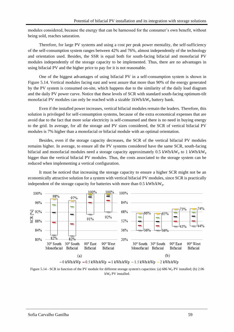
Potential of bifacial PV installation and its integration with storage solutions
Sofia Carvalho Ganilha 59
modules considered, because the energy that can be harnessed for the consumer’s own benefit, without
being sold, reaches saturation.
Therefore, for large PV systems and using a cost per peak power mentality, the self-sufficiency
of the self-consumption system ranges between 42% and 76%, almost independently of the technology
and orientation used. Besides, the SSR is equal both for south-facing bifacial and monofacial PV
modules independently of the storage capacity to be implemented. Thus, there are no advantages in
using bifacial PV and the higher price to pay for it is not reasonable.
One of the biggest advantages of using bifacial PV in a self-consumption system is shown in
Figure 5.14. Vertical modules facing east and west assure that more than 90% of the energy generated
by the PV system is consumed on-site, which happens due to the similarity of the daily load diagram
and the daily PV power curve. Notice that these levels of SCR with standard south-facing optimum-tilt
monofacial PV modules can only be reached with a sizable 1kWh/kWp battery bank.
Even if the installed power increases, vertical bifacial modules remain the leaders. Therefore, this
solution is privileged for self-consumption systems, because of the extra economical expenses that are
avoid due to the fact that more solar electricity is self-consumed and there is no need in buying energy
to the grid. In average, for all the storage and PV sizes considered, the SCR of vertical bifacial PV
modules is 7% higher than a monofacial or bifacial module with an optimal orientation.
Besides, even if the storage capacity decreases, the SCR of the vertical bifacial PV modules
remains higher. In average, to ensure all the PV systems considered have the same SCR, south-facing
bifacial and monofacial modules need a storage capacity approximately 0.5 kWh/kWp to 1 kWh/kWp
bigger than the vertical bifacial PV modules. Thus, the costs associated to the storage system can be
reduced when implementing a vertical configuration.
It must be noticed that increasing the storage capacity to ensure a higher SCR might not be an
economically attractive solution for a system with vertical bifacial PV modules, since SCR is practically
independent of the storage capacity for batteries with more than 0.5 kWh/kWp.
Figure 5.14 - SCR in function of the PV module for different storage system's capacities: (a) 686 Wp PV installed; (b) 2.06
kWp PV installed.
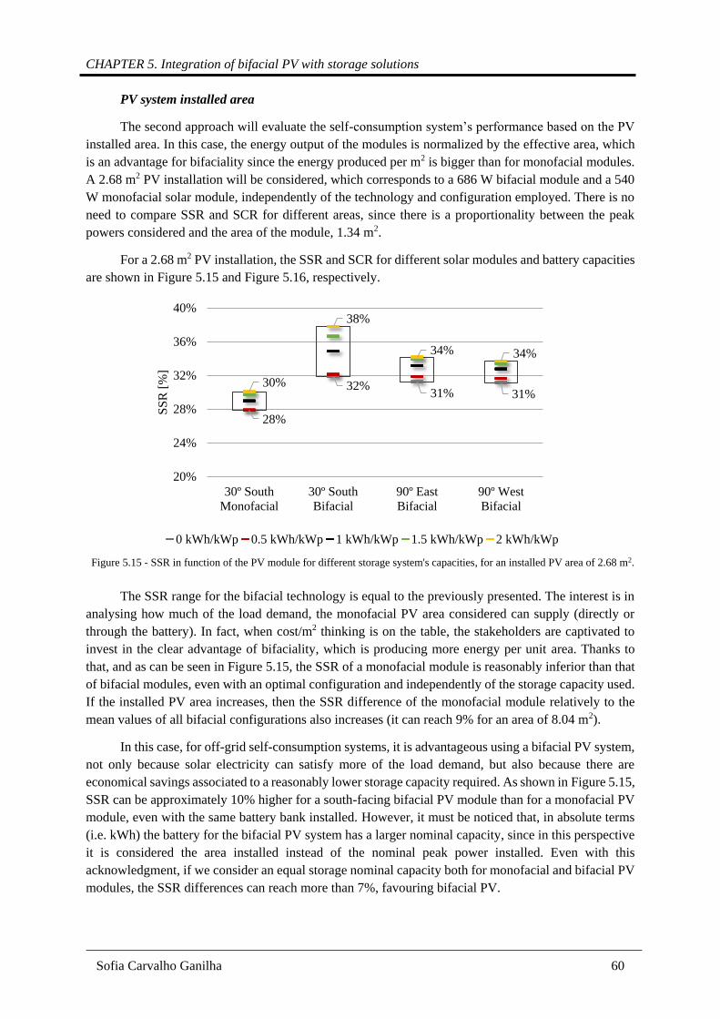
CHAPTER 5. Integration of bifacial PV with storage solutions
Sofia Carvalho Ganilha 60
PV system installed area
The second approach will evaluate the self-consumption system’s performance based on the PV
installed area. In this case, the energy output of the modules is normalized by the effective area, which
is an advantage for bifaciality since the energy produced per m2 is bigger than for monofacial modules.
A 2.68 m2 PV installation will be considered, which corresponds to a 686 W bifacial module and a 540
W monofacial solar module, independently of the technology and configuration employed. There is no
need to compare SSR and SCR for different areas, since there is a proportionality between the peak
powers considered and the area of the module, 1.34 m2.
For a 2.68 m2 PV installation, the SSR and SCR for different solar modules and battery capacities
are shown in Figure 5.15 and Figure 5.16, respectively.
The SSR range for the bifacial technology is equal to the previously presented. The interest is in
analysing how much of the load demand, the monofacial PV area considered can supply (directly or
through the battery). In fact, when cost/m2 thinking is on the table, the stakeholders are captivated to
invest in the clear advantage of bifaciality, which is producing more energy per unit area. Thanks to
that, and as can be seen in Figure 5.15, the SSR of a monofacial module is reasonably inferior than that
of bifacial modules, even with an optimal configuration and independently of the storage capacity used.
If the installed PV area increases, then the SSR difference of the monofacial module relatively to the
mean values of all bifacial configurations also increases (it can reach 9% for an area of 8.04 m2).
In this case, for off-grid self-consumption systems, it is advantageous using a bifacial PV system,
not only because solar electricity can satisfy more of the load demand, but also because there are
economical savings associated to a reasonably lower storage capacity required. As shown in Figure 5.15,
SSR can be approximately 10% higher for a south-facing bifacial PV module than for a monofacial PV
module, even with the same battery bank installed. However, it must be noticed that, in absolute terms
(i.e. kWh) the battery for the bifacial PV system has a larger nominal capacity, since in this perspective
it is considered the area installed instead of the nominal peak power installed. Even with this
acknowledgment, if we consider an equal storage nominal capacity both for monofacial and bifacial PV
modules, the SSR differences can reach more than 7%, favouring bifacial PV.
28%
32%31% 31%
30%
38%
34% 34%
20%
24%
28%
32%
36%
40%
30º South
Monofacial
30º South
Bifacial
90º East
Bifacial
90º West
Bifacial
SS
R [
%]
0 kWh/kWp 0.5 kWh/kWp 1 kWh/kWp 1.5 kWh/kWp 2 kWh/kWp
Figure 5.15 - SSR in function of the PV module for different storage system's capacities, for an installed PV area of 2.68 m2.
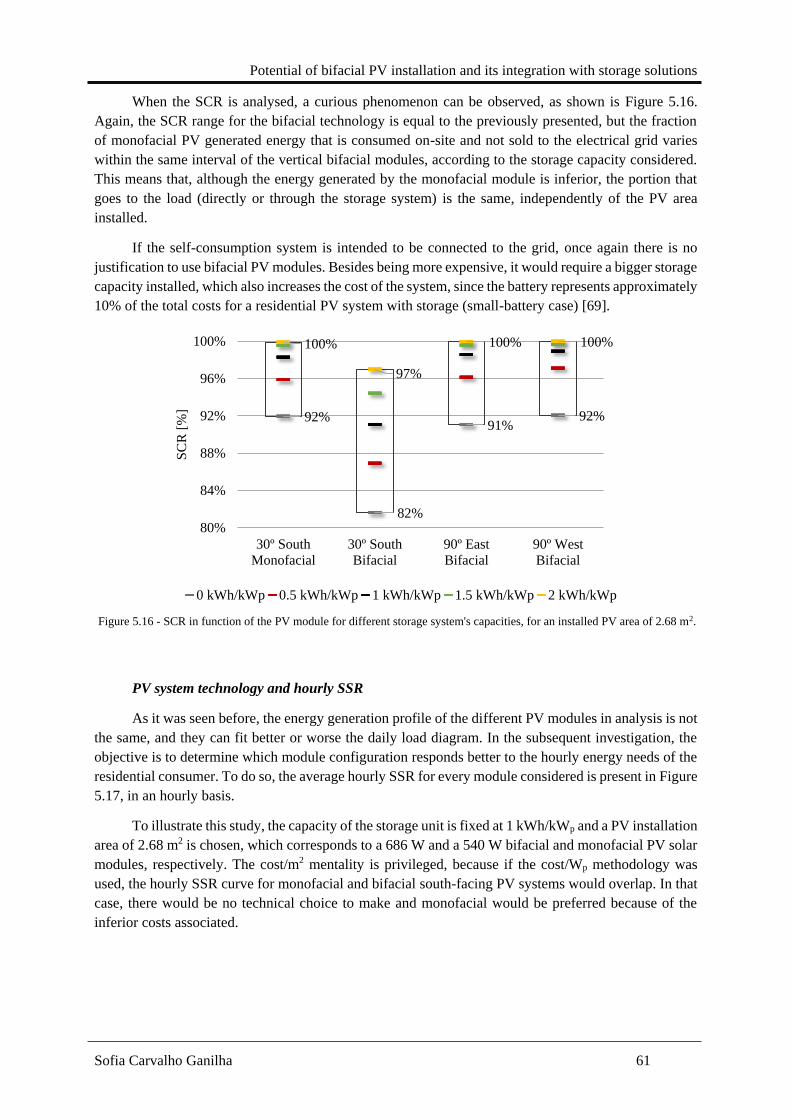
Potential of bifacial PV installation and its integration with storage solutions
Sofia Carvalho Ganilha 61
When the SCR is analysed, a curious phenomenon can be observed, as shown is Figure 5.16.
Again, the SCR range for the bifacial technology is equal to the previously presented, but the fraction
of monofacial PV generated energy that is consumed on-site and not sold to the electrical grid varies
within the same interval of the vertical bifacial modules, according to the storage capacity considered.
This means that, although the energy generated by the monofacial module is inferior, the portion that
goes to the load (directly or through the storage system) is the same, independently of the PV area
installed.
If the self-consumption system is intended to be connected to the grid, once again there is no
justification to use bifacial PV modules. Besides being more expensive, it would require a bigger storage
capacity installed, which also increases the cost of the system, since the battery represents approximately
10% of the total costs for a residential PV system with storage (small-battery case) [69].
PV system technology and hourly SSR
As it was seen before, the energy generation profile of the different PV modules in analysis is not
the same, and they can fit better or worse the daily load diagram. In the subsequent investigation, the
objective is to determine which module configuration responds better to the hourly energy needs of the
residential consumer. To do so, the average hourly SSR for every module considered is present in Figure
5.17, in an hourly basis.
To illustrate this study, the capacity of the storage unit is fixed at 1 kWh/kWp and a PV installation
area of 2.68 m2 is chosen, which corresponds to a 686 W and a 540 W bifacial and monofacial PV solar
modules, respectively. The cost/m2 mentality is privileged, because if the cost/Wp methodology was
used, the hourly SSR curve for monofacial and bifacial south-facing PV systems would overlap. In that
case, there would be no technical choice to make and monofacial would be preferred because of the
inferior costs associated.
Figure 5.16 - SCR in function of the PV module for different storage system's capacities, for an installed PV area of 2.68 m2.
92%
82%
91%92%
100%
97%
100% 100%
80%
84%
88%
92%
96%
100%
30º South
Monofacial
30º South
Bifacial
90º East
Bifacial
90º West
Bifacial
SC
R [
%]
0 kWh/kWp 0.5 kWh/kWp 1 kWh/kWp 1.5 kWh/kWp 2 kWh/kWp

CHAPTER 5. Integration of bifacial PV with storage solutions
Sofia Carvalho Ganilha 62
As can be seen in Figure 5.17, there are certain time periods of the day where implementing one
particular PV configuration can be more advantageous in order to meet the energy needs. During the
first sun hours, approximately until 9:00, vertical modules facing east or west have a higher SSR,
because their orientation enables the collection of direct radiation. However, SSR is slightly higher for
east-facing modules in this period, since the most efficient side is orientated to the sunrise. From 9:00
to 18:00, south bifacial solar modules can deliver (directly or through the battery) more energy to the
consumer. Lastly, in the latter hours of the day, after 18:00, verticality resumes the lead, because the
bifacial module is facing the sunset.
Even though the orientation can determine which module performs better in terms of matching
the production and demand, the technology type that consistently have the higher SSR is undoubtedly
bifacial PV. Combining modules with different orientations to achieve the highest SSR possible is an
attractive and feasible solution that helps softening the power production profile throughout the day.
For monofacial and bifacial modules facing south, the SSR is nearly symmetrical in relation to
12:00. Like the energy production curve shown in Figure 5.5, the hourly SSR profile during the day for
the vertical configurations in analysis also has two humps and, while the module turned to east performs
better in the morning, the west-facing solar module achieves a higher SSR during the afternoon.
For the system shown in the previous figure, the maximum SSR is 88% and is achieved only
between 11:00 and 12:00. Nevertheless, if the PV installation area increases, the PV power production
also grows and more energy can be used to immediately suppress the residential energy demand or to
charge the battery to be used when required, extending the self-sufficiency period between 5:00 and
21:00. For example, for an area of 8.04 m2, almost 100% of the load demand comes from PV generated
energy between 8:00 and 16:00, independently of the configuration used.
In turn, if the storage system capacity increases, only the self-sufficiency period widens, because
more energy can be stored to be used in periods of need. However, the maximum SSR achievable is the
same.
Concluding, a better fit to the residential energy needs can be obtained through the combination
of bifacial modules with different orientations. If a higher storage system capacity and PV area
installation are chosen, then SSR increases, as well as the time period during which is possible for the
0%
20%
40%
60%
80%
100%S
SR
[%
]
30º South Monofacial 30º South Bifacial 90º East Bifacial 90º West Bifacial
Figure 5.17 – Mean average of the hourly SSR for the different modules’ types and configurations considered, a storage
capacity of 1 kWh/kWp and a PV installation area of 2.68 m2.
Potential of bifacial PV installation and its integration with storage solutions
Sofia Carvalho Ganilha 63
consumer to be self-sufficient, what is intended especially for self-consumption solutions isolated from
the electrical grid.
Final notes
All the previous self-consumption systems have been simulated and analysed without considering
practical economical constrains. However, when investing in a project like this, the economical
evaluation is a key element to help making a decision. In order to access this type of analysis, the costs
of the PV system (investment, operation and maintenance), of the battery (including the replacement
costs) and the price of the electricity from grid must be considered, as well as the “green” financial
incentives and the sale price of the energy generated by RES.
In this dissertation, it was chosen to study a self-consumption solution for a residential consumer,
mainly to investigate the better match between the daily load diagram and the power PV generation
curve of a bifacial module in a vertical position facing either east or west. Besides, since no economic
considerations were taken into account, bifacial technology performs always better than the traditional
monofacial PV, especially in this type of applications, where the installation area plays an important
role. As a consequence, even if the consumption profile for commercial or services sectors, for example,
was considered (in this case the peak demand coincides with the PV power peak), SSR would be higher
for bifacial solar modules. Nevertheless, if the self-consumption system implemented in the
aforementioned sectors was intended to be connected to the electrical grid, probably a higher SCR would
be achieved using monofacial PV modules and, therefore, the choice would probably be on this
technology.
CHAPTER 6. Conclusion and further work
Sofia Carvalho Ganilha 64
6. Conclusion and further work
Making photovoltaic systems more affordable and cost competitive is the main driver to continue
the research for new devices and concepts able to convert solar radiation more efficiently. The
investigations seek new ways of generating more electricity throughout the PV systems’ lifetime
associated to a decrease of their costs over the same period. Bifacial PV is one of the concepts proposed
to reach those objectives, although it requires the implantation of a new paradigm, mainly focused on
the energy converted by unit area and not by Watt peak. Conceptually, the savings are achieved by the
possibility to install a higher PV power capacity within the same area as a monofacial system, able to
take advantage of the incident reflected and diffuse radiation that reaches the rear surface of the PV
module and, consequently, increasing the generated electricity. The potential of using bifacial PV was
briefly reviewed in Chapter 2, where bifacial gains of 54% and 25% were already reported for single
modules and small testing systems, respectively.
The research aim of this dissertation was to compare the responses of bifacial solar modules with
monofacial PV modules, in terms of incident irradiation, electricity generation and integration in a
residential self-consumption system with storage. Based on these raw theoretical results, bifacial gains
were quantified and the optimal configuration of a single bifacial module and a PV system was proposed.
The irradiance model, described in Chapter 3.1, was based on the “Ray-tracing Method” and was
developed in Rhinoceros®, using the energy modelling plug-in DIVA®. To quantify the incident
irradiation differences between bifacial and monofacial modules, a new quantity was introduced, IBG,
defined as the ratio between the rear and front irradiances. A bifacial PV system is more sensitive to the
stand configuration and external neighbouring factors than a monofacial PV system. For this reason, the
study explored the impact of the variables that directly affect the amount of radiation collected by the
solar module and, consequently, the energy output, such as the ground’s albedo, the elevation and tilt
angle of the module, the landscape versus portrait position and the inter-row and within row spacings.
A directly proportional relation between the IBG and the ground’s albedo was confirmed, which
may justify the initial investment in a highly reflective surface and the corresponding maintenance costs.
This dependency is more intense for low tilt angles and bigger elevations.
As the elevation of the module increases, the increase of both IBG and the rear annual radiation
is similar, because the self-shadowing effect of the rear side of the module decreases and the intercepted
diffuse radiation increases, as the radiation collected by the front side remains practically the same.
Above a certain elevation, the IBG saturates and there is no reason to invest in more complex and
expensive mounting structures for higher stands. The saturation height is lower for landscaped modules
with a very pronounced tilt angle and above a surface with low albedo.
It was also seen that the irradiation intercepted by the rear side of a portrait module is more
inhomogeneous, albeit more intense and with a higher IBG (additional 1% to 2%), comparatively to
landscape modules. Hence, the mounting position affects the electrical output of the module.
The optimal tilt angle that maximizes the total intercepted irradiation is generally different from
the one that optimises the IBG. Highest IBG are achieved with almost vertical tilt angles, to conciliate
the incident radiation boost on the rear side with a decrease of the radiation intercepted by the front side
of the module. In order to improve the total irradiation collection, the tilt angle must be slightly higher
than in the monofacial case, to take advantage of the incident irradiation on the rear side of the module.

Potential of bifacial PV installation and its integration with storage solutions
Sofia Carvalho Ganilha 65
The difference between the optimum tilt angles for bifacial and monofacial modules is more accentuated
for highly reflective ground surfaces.
The IBG varied from 5%, corresponding to a module with low elevation and slope above grass,
to 70%, for highly reflective surfaces and a module far from the ground, independently of being in a
portrait or landscape mounting.
For a system with more than one module, the ideal distances between rows and between modules
within a row were determined to minimize cross shading. For less reflective grounds, the ideal inter-row
spacing is equal for monofacial and bifacial solar modules, with less than 5% losses above 1.5 meters.
As the albedo increases, to keep the loss below 5% requires larger spacings between rows of bifacial
modules. For highly reflective ground surfaces, the ideal inter-row spacing can exceed almost 2.25
meters, which is clearly a disadvantage for this technology.
The ideal distance within a row is a variable of low relevance for monofacial modules and bifacial
solar modules above surfaces with low albedo. Nevertheless, as the ground’s albedo increases, the
modules should be separated to guarantee that the shadows of the neighbouring solar modules do not
affect the energy received. The mutual shading is negligible (less than 5%) for module’s spacing above
0.5 m.
Optimizing the design of a bifacial PV system is not simple, since there is a compromise between
the maximization of the energy yield and the cost minimization. For example, the higher mounting
structure for modules is more expensive and the artificial ground with a high reflectivity will increase
its maintenance costs [27].
If economic factors are considered, the optimal design of the bifacial PV stand will simultaneously
maximize the total production and the specific production [28]. Comparatively to monofacial PV power
plants, the distance between and within rows for a bifacial system ought to be increased, as well as the
module’s elevation and tilt angle. These design specifications have a direct impact on the investment.
On the other hand, their energy yield per unit area is higher for bifacial modules and therefore it is not
very clear in which conditions, if any, the bifacial LCOE estimation might be competitive to the
monofacial LCOE [28].
The electrical model, described in Chapter 4, was inspired in the method proposed by Singh et al.
to characterize bifacial PV modules as the parallel of two one-diode model solar cells, hence assuming
that the front and rear sides of a bifacial solar cell are independent. This assumption can lead to slight
deviations between simulation results and experimentally collected data, since it does not consider the
interaction between the two sides. The model constructed to estimate the hourly power output of a PV
module was developed in MATLAB Simulink® and was tested for different orientations, tilt angles and
mounting positions (landscape versus portrait) of the module.
First of all, it is important to highlight the proportionality between the irradiation (IBG) and the
energy (EBG) bifacial gains, since it implies that the boost for the collected irradiation discussed in
Chapter 3 can be extrapolated in terms of the energy output. However, this proportionality does not
assure that the optimum IBG configuration also maximizes the overall energy conversion. Indeed, the
optimum tilt angle for a bifacial module was found to be very similar to the monofacial case.
It was also observed that EBG increases with the diffuse fraction. This behaviour is clearly
detected when assessing the daily variation of the EBG, because higher EBG is reached when the diffuse
fraction is higher (sunrise and sunset) since the contribution of the irradiance on the back of the module
is higher comparatively to the front side.

CHAPTER 6. Conclusion and further work
Sofia Carvalho Ganilha 66
Relatively to the mounting positions (landscape versus portrait), the conclusions made in Chapter
3 were confirmed, as there is an annual slightly advantage for landscape modules. The smallness of the
effect indicates that the amplitude and gradient of the front irradiation overlays the rear surface effects.
In quantitative terms, the EBG varies between 28% and 35%, depending on the tilt angle.
However, if the aforementioned comparisons are done independently of the power capacity of the PV
solar module, i.e. the power output is normalized by the peak capacity of the module, there is almost no
advantage in choosing bifacial over monofacial, especially due to economic factors.
Regarding to the module’s orientation, a peak-shifting effect can be obtained when bifacial PV
modules are installed vertically and oriented towards east/west. In these cases, two humps can be
visualized at dawn and twilight.
Chapter 5 explores the dynamic and performance of a residential self-consumption PV system,
with different levels of storage capacity, assessed using two indicators: the self-consumption rate (SCR)
and the self-sufficiency rate (SSR). The first one is relevant for systems connected to the electrical grid
and quantifies the fraction of generated PV energy that is consumed on-site. The second one is more
relevant for off-grid systems, because it determines how much of the electrical demand the PV system
can supply (directly or through the storage unit). For this study, four PV systems were analysed,
considering different modules’ technologies (monofacial or bifacial) and configurations (orientation and
tilt angle). For simulation purposes, a typical residence with an annual demand of 2 890.25 kWh was
considered.
To analyse which PV technology and configuration is better to implement in a self-consumption
solution, two different approaches were used. The first one considers that the energy output of the
monofacial module is normalized by the peak power, forcing it to approximately produce as much as
the bifacial south-facing system. The second one evaluates the self-consumption system’s performance
based on the PV effective area, i.e. the energy output of the modules is normalized by the module’s area.
Using the first approach, it was seen that there is almost no difference in using south-facing
bifacial or monofacial modules. If the interest is in a system isolated from the electrical grid, then,
technically, either bifacial or monofacial solar modules south-facing could be chosen, increasing the PV
power and storage capacity installed. In the best-case scenario studied, 76% of the energy needs are
assured by PV generation. For off-grid self-consumption systems, SSR is higher but practically the same
for monofacial and bifacial PV modules with an optimal orientation and tilt angle.
For self-consumption systems connected to the electrical grid, bifacial modules towards east or
west can assure that more than 90% of the PV generation is consumed on-site, which also enables a
decrease of the storage capacity and the PV power installed. The storage capacity can be decreased by
more than 1 kWh/kWp relatively to south facing (monofacial or bifacial) PV modules.
Per unit area, the performance of the bifacial PV system is even more advantageous: to ensure the
same SSR, a monofacial PV system would require at least a storage capacity +2 kWh/kWp higher than
if the modules were bifacial and south-facing. Vertical bifacial modules would require an intermediate
storage capacity +1 kWh/kWp higher than south-facing tilted bifacial modules.
For self-consumption systems connected to the electrical grid, the choice is not so clear between
vertical bifacial modules facing east or west and a south-facing monofacial module, since both
configurations have similar SCR, independently of the PV area installed. In this case, the choice would
be economical and monofacial technology would certainly be the appropriate choice.

Potential of bifacial PV installation and its integration with storage solutions
Sofia Carvalho Ganilha 67
Finally, there are specific time periods of the day where a certain PV configuration can be more
advantageous in order to meet the load demand. Therefore, the combination of bifacial modules with
different orientations can not only soften the power production profile throughout the day, but also
extend the self-sufficiency period.
During the simulations and the analysis of the results, the assumptions and simplifications made
were always kept in mind, because they intrinsically influence the outcomes and conclusions. The
simplifications include the absence of the mounting structure and the junction box, which, when
considered, introduce more shadow effects to be analysed, and this influences the radiation gradient on
both sides of the PV module. Also, the electrical model was developed based on a pre-existent datasheet,
and the electrical parameters could not be experimentally confirmed. In addiction, the shunt resistance
was neglected due to the same difficulty expressed before, thus some losses were not quantified.
Further work
The validation of the theoretical results exposed in this dissertation with experimental data from
the future facility to test bifacial PV is of utmost importance, in order to develop and upgrade an
analytical model that can accurately estimate the energy output, independently of the location and time
of year. Unfortunately, the experimental setup was not deployed on time for analysis in this dissertation.
As it was already stated, the electrical parameters should be determined experimentally and the
temperature of the modules should be monitored, e.g. by sensors or IR thermography for each one of
the solar cells.
After addressing the principal limitations of the irradiance and electrical models, an economic
analysis should be done. This way, the bifaciality will be analysed not only in terms of energy, but also
in terms of economic factors that can influence the investment of stakeholders. This study ought to be
complemented by sensitivity analysis, identifying the cost thresholds that enable economic viability of
bifacial PV modules.

CHAPTER 7. Bibliographic references
Sofia Carvalho Ganilha 68
7. Bibliographic references
[1] J. L. Sawin et al. Renewables 2017: Global Status Report. REN21. 2017.
[2] C. Philibert et al. Technology Roadmap - Solar Photovoltaic Energy. International Energy
Agency IEA. 2014.
[3] A. Hauser, A. Richter, and S. Leu. Cell and module design from the LCOE perspective.
Meyer Burger Technology Ltd., 2014.
[4] A. Halm et al. The Zebra cell concept - Large area n-type interdigitated back contact solar
cells and one-cell modules fabricated using standard industrial processing equipment. Proceeding 27th
Eur. Photovolt. Sol. Energy Conf. Exhib. Frankfurt, Ger., pp. 567–570. 2012.
[5] Mori H. U.S. patent No. 3278811A; October 1966.
[6] S. Chunduri and M. Schmela, Bifacial Solar Module Technology. TaiyanNews. 2017.
[7] A. Cuevas. The early history of bifacial solar cells. 20th European PV solar energy
conference, pp. 801–805. 2005.
[8] WIPO, “WIPO - World Intellectual Property Organization”, PCT – The International
Patent System, 2015.
[9] R. Kopecek and Y. Veschetti. Bifaciality: One small step for technology, one giant leap for
kWh cost reduction. Photovoltaics Int., vol. 26, pp. 32–45. 2015.
[10] N. Ishikawa and S. Nishiyama. World First Large Scale 1.25MW Bifacial PV Power Plant
on Snowy Area in Japan. 3rd Bifacial PV Workshop. 2016.
[11] J. Libal and R. Kopecek. Review of Bifacial PV Systems. 3rd Bifacial PV Workshop. 2016.
[12] Yingli Connects a 50 MW "Top Runner" PV Project in Shanxi Province, China to the Grid.
Yingli Green Energy Holding Company Limited. 2016. URL: http://www.prnewswire.com/news-
releases/yingli-connects-a-50-mw-top-runner-pv-project-in-shanxi-province-china-to-the-grid-
300293164.html (visited on 8/August/2017).
[13] Opening of Europe's Largest Bifacial Solar PV Plant in the Netherlands. Yingli Green
Energy Holding Company Limited. 2017. URL: http://www.prnewswire.com/news-releases/opening-
of-europes-largest-bifacial-solar-pv-plant-in-the-netherlands-300472168.html (visited on
8/August/2017).
[14] R. Kopecek and J. Libal. Quo vadis bifacial PV?. Photovoltaics Int., vol. 35, pp. 86–91.
2017.
[15] International Technology Roadmap for Photovoltaic – 2016 Results. ITRPV. 2017.
[16] D. Brearley. Bifacial PV Systems. SolarPro magazine. 2017. URL:
http://solarprofessional.com/articles/design-installation/bifacial-pv-systems (visited on 8/August/2017).
[17] R. Guerrero-Lemus et al. Bifacial solar photovoltaics - a technology review. Renew.
Sustain. Energy Rev., vol. 60, pp. 1533–1549. 2016.

Potential of bifacial PV installation and its integration with storage solutions
Sofia Carvalho Ganilha 69
[18] C. Comparotto et al. Energy Yield Estimation of Monofacial and Bifacial Solar Modules.
31st European Photovoltaic Solar Energy Conference and Exhibition, pp. 1858–1862. 2015.
[19] G. Razongles et al. Bifacial Photovoltaic Modules: Measurement Challenges. Energy
Procedia, vol. 92, pp. 188–198. 2016.
[20] R. Kopecek, I. Shoukry, and J. Libal. Cost/kWh thinking and bifacialty: Two allies for low-
cost PV of the future. Photovoltaics Int., vol. 4th Quarte, pp. 88–97. 2015.
[21] SolarWorld’s Mono-PERC Bifacial Modules on Way to University of Richmond Test Bed.
SolarWorld Americas Inc. 2017. URL:
http://www.businesswire.com/news/home/20160307005250/en/SolarWorld%E2%80%99s-Mono-
PERC-Bifacial-Modules-University-Richmond-Test (visited on 8/August/2017).
[22] ISC Konstanz and MegaCell Sign License Agreement. MegaCell. 2014. URL:
http://www.mega-group.it/megacell/en/news-megacell-en/2790-isc-konstanz-and-megacell-sign-
license-agreement/ (visited on 8/August/2017).
[23] A. Jäger-Waldau. Snapshot of photovoltaics-March 2017. Sustainability, vol. 9, no. 5.
2017.
[24] D. Jimenez. Cost of ownership and overall equipment efficiency: a photovoltaics
perspective. Photovoltaics Int., vol. 4, pp. 16–22, 2009.
[25] M. Marzoli et al. Field Performance Assessment and Comparison of Mono & Bifacial PV
Modules. 2015.
[26] P. Dupeyrat et al. Investigations on Albedo Dependency of Bifacial PV Yield. 2014.
[27] S. Wendlandt et al. Realistic Yield Expectations for Bifacial PV Systems – an Assessment
of Announced, Predicted and Observed Benefits. 2015.
[28] A. Lindsay et al. Key Elements in the Design of Bifacial PV Power Plants. 31st European
Photovoltaic Solar Energy Conference and Exhibition, pp. 1764–1769. 2015.
[29] B. Marion, S. Macalpine, and C. Nrel. A Practical Irradiance Model for Bifacial PV
Modules. 2017.
[30] I. Shoukry et al. Modelling of Bifacial Gain for Stand-alone and in-field Installed Bifacial
PV Modules. Energy Procedia, vol. 92, pp. 600–608. 2016.
[31] U. A. Yusufoglu et al. Analysis of the annual performance of bifacial modules and
optimization methods. IEEE J. Photovoltaics, vol. 5, no. 1, pp. 320–328. 2015.
[32] J. Appelbaum. Bifacial photovoltaic modules field. Renew. Energy, vol. 85, pp. 338–343.
2016.
[33] P. G. Loutzenhiser et al. Empirical validation of models to compute solar irradiance on
inclined surfaces for building energy simulation. Sol. Energy, vol. 81, no. 2, pp. 254–267. 2007.
[34] C. Deline, S. Macalpine, B. Marion, and J. S. Stein. Evaluation and Field Assessment of
Bifacial Photovoltaic Module Power Rating Methodologies. 43rd IEEE Photovolt. Spec. Conf. 5-10
June 2016, Portland, Oregon, no. June. 2016.

CHAPTER 7. Bibliographic references
Sofia Carvalho Ganilha 70
[35] M. Chiodetti et al. Enhancing Bifacial PV Modelling with Ray-tracing. 6th PV
Performance Modeling Collaborative Workshop. 2016.
[36] A. Smets et al. Solar Cell Parameters and Equivalent Circuit. Sol. Energy Phys. Eng.
Photovolt. conversion, Technol. Syst., pp. 111–124. 2016.
[37] S. Suckow, T. M. Pletzer, and H. Kurz. Fast and reliable calculation of the two-diode
model without simplifications. Prog. Photovoltaics,vol. 22, pp. 494–501. 2014.
[38] J. P. Singh, A. G. Aberle, and T. M. Walsh. Electrical characterization method for bifacial
photovoltaic modules. Sol. Energy Mater. Sol. Cells, vol. 127, pp. 136–142. 2014.
[39] Y. K. Chieng and M.A. Green. Computer Simulation of Enhanced Output from Bifacial
Photovoltaic Modules. Progress in photovoltaics: research and applications vol. 1, pp. 293–299. 1993.
[40] T. Mrabti, M. El Ouariachi, and B. T. K. Kassmi. Caractérisation et modélisation fine du
fonctionnement électrique des panneaux photovoltaïques. 2009.
[41] J. Johnson, D. Yoon, and Y. Baghzouz. Modeling and analysis of a bifacial grid-connected
photovoltaic system. IEEE Power Energy Soc. Gen. Meet., pp. 1–6. 2012.
[42] A. Hübner, A. Aberle, and R. Hezel. Temperature behavior of monofacial and bifacial
silicon solar cells. Conf. Rec. Twenty Sixth IEEE Photovolt. Spec. Conf. - 1997, pp. 223–226. 1997.
[43] Calculating the Additional Energy Yield of Bifacial Solar Modules. SolarWorld. 2015.
[44] NOCT definition. PVsyst – Photovoltaic Software. 2014. URL:
http://files.pvsyst.com/help/noct_definition.htm (visited on 8/August/2017).
[45] D. L. King, W. E. Boyson, and J. A. Kratochvil. Photovoltaic array performance model.
Sandia Rep. No. 2004-3535, vol. 8, no. December, pp. 1–19. 2004.
[46] H. Nussbaumer et al. PV Installations Based on Vertically Mounted Bifacial Modules. 31st
European Photovoltaic Solar Energy Conference and Exhibition, pp. 2029–2033. 2015.
[47] T. Joge et al. Basic application technologies of bifacial photovoltaic solar modules. Electr.
Eng. Japan (English Transl. Denki Gakkai Ronbunshi), vol. 149, no. 3, pp. 32–42. 2004.
[48] S. Freitas and M. C. Brito. Bifacial PV integrated on building balconies. 2016.
[49] B. Soria, E. Gerritsen, and P. Lefillastre. Vertical Façade Integration of Bifacial PV
Modules: Outdoor Testing & Optical Modeling. 28th European Photovoltaic Solar Energy Conference
and Exhibition, pp. 3216–3221. 2013.
[50] S. Guo, T. M. Walsh, and M. Peters. Vertically mounted bifacial photovoltaic modules: a
global analysis. Energy, vol. 61, pp. 447–454. 2013.
[51] EnergyPlus (2017). URL: https://energyplus.net/weather (visited on 8/August/2017).
[52] Rhinoceros 3D (2017). URL: http://www.rhino3d.com (visited on 8/August/2017).
[53] Diva For Rhino (2017). URL: http://diva4rhino.com (visited on 8/August/2017).
[54] D. Robinson and A. Stone. Irradiation modelling made simple: the cumulative sky
approach and its applications. PLEA - Passiv. Low Energy Archit. Eindhoven, Netherlands, no.
September, pp. 19–22. 2004.
Potential of bifacial PV installation and its integration with storage solutions
Sofia Carvalho Ganilha 71
[55] Lighting Materials for Simulation. URL: http://www.lighting-materials.com (visited on
8/August/2017).
[56] R. Guerrero-Lemus, R. Vega, T. Kim, A. Kimm, and L. E. Shephard. Bifacial solar
photovoltaics - A technology review. Renew. Sustain. Energy Rev., vol. 60, pp. 1533–1549. 2016.
[57] Design Guide for Bifacial Solar Modules Design Guide for Bifacial Solar Modules.
PrismSolar Technologies, Inc.
[58] Simscape Blocks: Solar Cell. MathWorks documentation. 2014. URL:
https://www.mathworks.com/help/physmod/elec/ref/solarcell.html (visited on 8/August/2017).
[59] Datasheet PrismSolar® Bi60-343BSTC.
[60] Krismadinata, N. A. Rahim, H. W. Ping, and J. Selvaraj. Photovoltaic Module Modeling
using Simulink/Matlab. Procedia Environ. Sci., vol. 17, pp. 537–546. 2013.
[61] MINISTÉRIO DO AMBIENTE ORDENAMENTO DO TERRITÓRIO. Produção de
Energia Distribuída: Decreto-Lei n.o 153/2014. Diário da República - I Série, vol. N.o 202, pp. 5298–
5311. 2014.
[62] V. A. Reis. Community storage for small urban units including dwelling and small
businesses. Faculdade de Ciências da Universidade de Lisboa. Dissertação de mestrado, 2017.
[63] S. Quoilin et al. Quantifying self-consumption linked to solar home battery systems:
statistical analysis and economic assessment. Applied Energy 182, pp. 58–67. 2016.
[64] Guia de Medição, Leitura e Disponibilização de Dados. ERSE. 2016.
[65] Informação de Mercado: Perfis de Consumo. REN – Sistema de Informação de Mercados
de Energia. 2015. URL:
http://www.mercado.ren.pt/PT/Electr/InfoMercado/Consumo/Paginas/PerfisConsumo.aspx (visited on
8/August/2017).
[66] PORDATA – Base de Dados Portugal Contemporâneo. URL: http://www.pordata.pt/Home
(visited on 8/August/2017).
[67] D. Linden and T. B. Reddy. Handbook of batteries. Third Edit. McGraw-Hill, 2004.
[68] SMA Solar Technology SG. URL: http://www.sma.de/en.html (visited on 8/August/2017).
[69] K. Ardani et al. Installed Cost Benchmarks and Deployment Barriers for Residential Solar
Photovoltaics with Energy Storage: Q1 2016. NREL. 2016
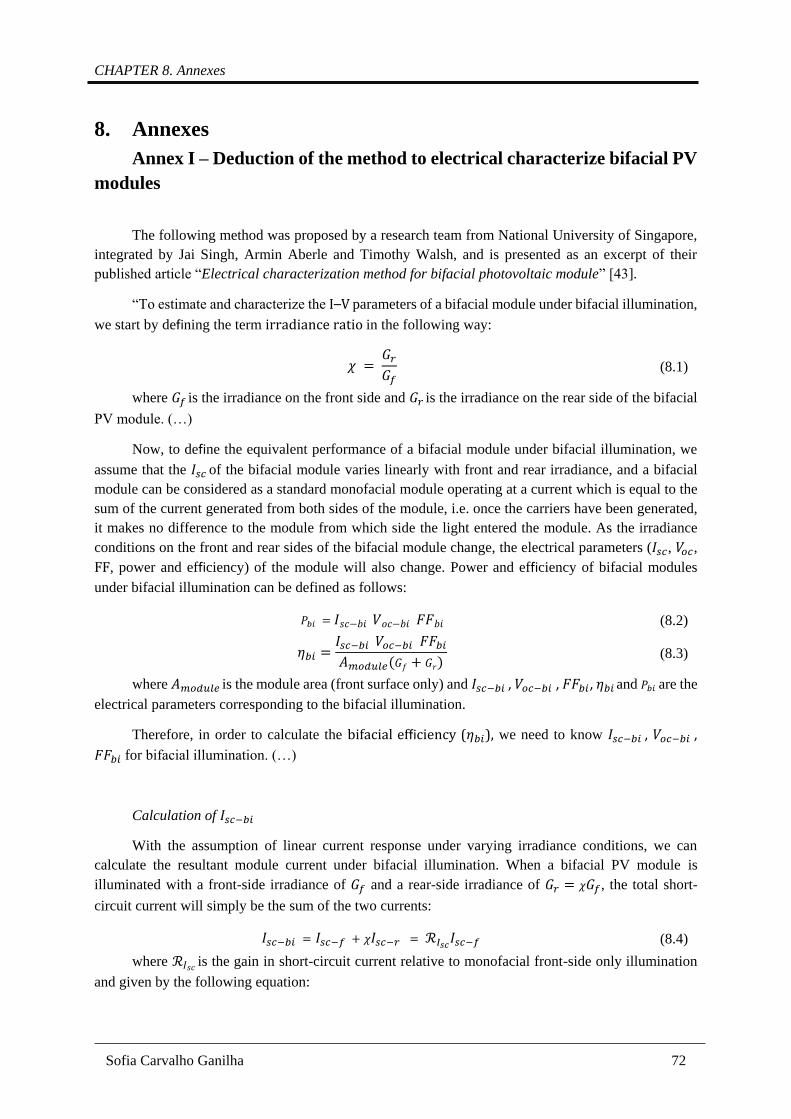
CHAPTER 8. Annexes
Sofia Carvalho Ganilha 72
8. Annexes
Annex I – Deduction of the method to electrical characterize bifacial PV
modules
The following method was proposed by a research team from National University of Singapore,
integrated by Jai Singh, Armin Aberle and Timothy Walsh, and is presented as an excerpt of their
published article “Electrical characterization method for bifacial photovoltaic module” [43].
“To estimate and characterize the I–V parameters of a bifacial module under bifacial illumination,
we start by defining the term irradiance ratio in the following way:
𝜒 = 𝐺𝑟
𝐺𝑓 (8.1)
where 𝐺𝑓 is the irradiance on the front side and 𝐺𝑟 is the irradiance on the rear side of the bifacial
PV module. (…)
Now, to define the equivalent performance of a bifacial module under bifacial illumination, we
assume that the 𝐼𝑠𝑐 of the bifacial module varies linearly with front and rear irradiance, and a bifacial
module can be considered as a standard monofacial module operating at a current which is equal to the
sum of the current generated from both sides of the module, i.e. once the carriers have been generated,
it makes no difference to the module from which side the light entered the module. As the irradiance
conditions on the front and rear sides of the bifacial module change, the electrical parameters (𝐼𝑠𝑐, 𝑉𝑜𝑐,
FF, power and efficiency) of the module will also change. Power and efficiency of bifacial modules
under bifacial illumination can be defined as follows:
𝑃𝑏𝑖 = 𝐼𝑠𝑐−𝑏𝑖 𝑉𝑜𝑐−𝑏𝑖 𝐹𝐹𝑏𝑖 (8.2)
𝜂𝑏𝑖 =𝐼𝑠𝑐−𝑏𝑖 𝑉𝑜𝑐−𝑏𝑖 𝐹𝐹𝑏𝑖
𝐴𝑚𝑜𝑑𝑢𝑙𝑒(𝐺𝑓 + 𝐺𝑟) (8.3)
where 𝐴𝑚𝑜𝑑𝑢𝑙𝑒 is the module area (front surface only) and 𝐼𝑠𝑐−𝑏𝑖 , 𝑉𝑜𝑐−𝑏𝑖 , 𝐹𝐹𝑏𝑖, 𝜂𝑏𝑖 and 𝑃𝑏𝑖 are the
electrical parameters corresponding to the bifacial illumination.
Therefore, in order to calculate the bifacial efficiency (𝜂𝑏𝑖), we need to know 𝐼𝑠𝑐−𝑏𝑖 , 𝑉𝑜𝑐−𝑏𝑖 ,
𝐹𝐹𝑏𝑖 for bifacial illumination. (…)
Calculation of 𝐼𝑠𝑐−𝑏𝑖
With the assumption of linear current response under varying irradiance conditions, we can
calculate the resultant module current under bifacial illumination. When a bifacial PV module is
illuminated with a front-side irradiance of 𝐺𝑓 and a rear-side irradiance of 𝐺𝑟 = 𝜒𝐺𝑓, the total short-
circuit current will simply be the sum of the two currents:
𝐼𝑠𝑐−𝑏𝑖 = 𝐼𝑠𝑐−𝑓 + 𝜒𝐼𝑠𝑐−𝑟 = ℛ𝐼𝑠𝑐𝐼𝑠𝑐−𝑓 (8.4)
where ℛ𝐼𝑠𝑐 is the gain in short-circuit current relative to monofacial front-side only illumination
and given by the following equation:
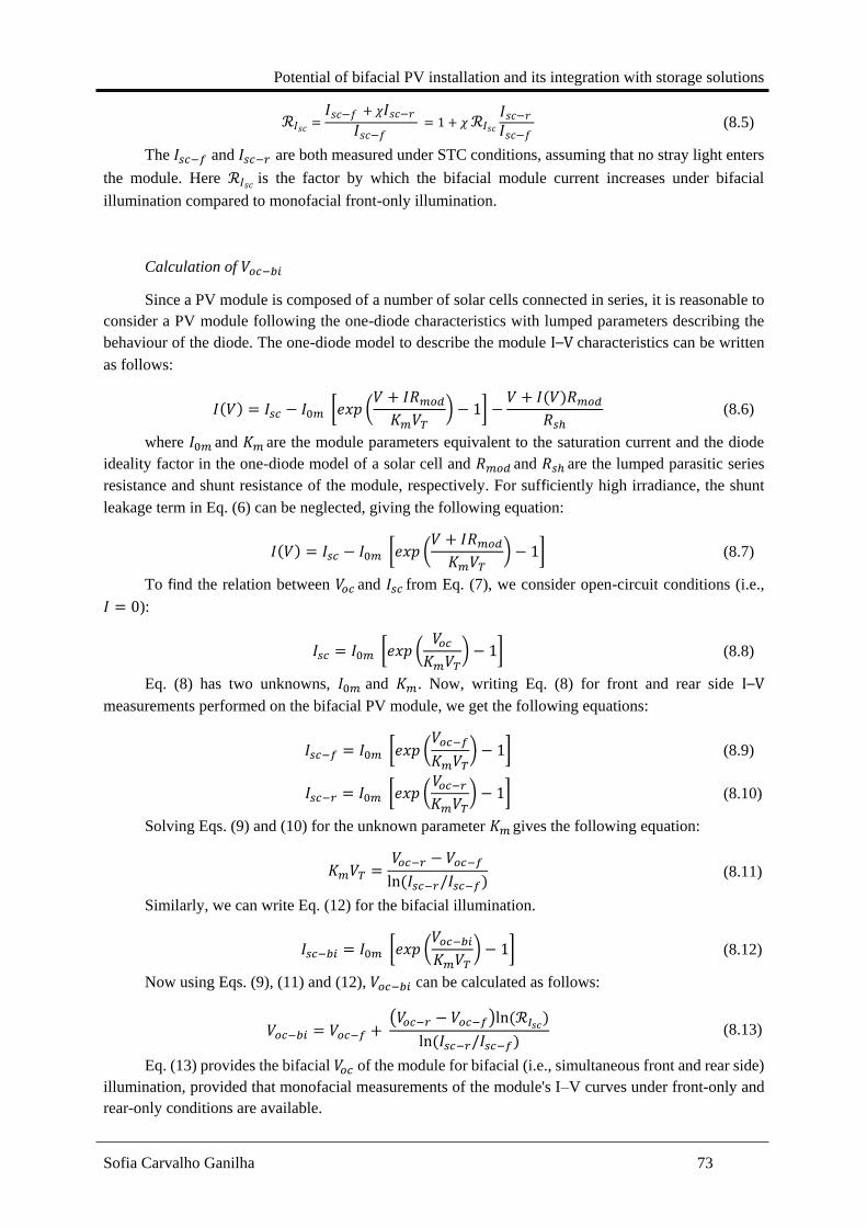
Potential of bifacial PV installation and its integration with storage solutions
Sofia Carvalho Ganilha 73
ℛ𝐼𝑠𝑐=
𝐼𝑠𝑐−𝑓 + 𝜒𝐼𝑠𝑐−𝑟
𝐼𝑠𝑐−𝑓 = 1 + 𝜒 ℛ𝐼𝑠𝑐
𝐼𝑠𝑐−𝑟
𝐼𝑠𝑐−𝑓 (8.5)
The 𝐼𝑠𝑐−𝑓 and 𝐼𝑠𝑐−𝑟 are both measured under STC conditions, assuming that no stray light enters
the module. Here ℛ𝐼𝑠𝑐 is the factor by which the bifacial module current increases under bifacial
illumination compared to monofacial front-only illumination.
Calculation of 𝑉𝑜𝑐−𝑏𝑖
Since a PV module is composed of a number of solar cells connected in series, it is reasonable to
consider a PV module following the one-diode characteristics with lumped parameters describing the
behaviour of the diode. The one-diode model to describe the module I–V characteristics can be written
as follows:
𝐼(𝑉) = 𝐼𝑠𝑐 − 𝐼0𝑚 [𝑒𝑥𝑝 (𝑉 + 𝐼𝑅𝑚𝑜𝑑
𝐾𝑚𝑉𝑇) − 1] −
𝑉 + 𝐼(𝑉)𝑅𝑚𝑜𝑑
𝑅𝑠ℎ (8.6)
where 𝐼0𝑚 and 𝐾𝑚 are the module parameters equivalent to the saturation current and the diode
ideality factor in the one-diode model of a solar cell and 𝑅𝑚𝑜𝑑 and 𝑅𝑠ℎ are the lumped parasitic series
resistance and shunt resistance of the module, respectively. For sufficiently high irradiance, the shunt
leakage term in Eq. (6) can be neglected, giving the following equation:
𝐼(𝑉) = 𝐼𝑠𝑐 − 𝐼0𝑚 [𝑒𝑥𝑝 (𝑉 + 𝐼𝑅𝑚𝑜𝑑
𝐾𝑚𝑉𝑇) − 1] (8.7)
To find the relation between 𝑉𝑜𝑐 and 𝐼𝑠𝑐 from Eq. (7), we consider open-circuit conditions (i.e.,
𝐼 = 0):
𝐼𝑠𝑐 = 𝐼0𝑚 [𝑒𝑥𝑝 (𝑉𝑜𝑐
𝐾𝑚𝑉𝑇) − 1] (8.8)
Eq. (8) has two unknowns, 𝐼0𝑚 and 𝐾𝑚. Now, writing Eq. (8) for front and rear side I–V
measurements performed on the bifacial PV module, we get the following equations:
𝐼𝑠𝑐−𝑓 = 𝐼0𝑚 [𝑒𝑥𝑝 (𝑉𝑜𝑐−𝑓
𝐾𝑚𝑉𝑇) − 1] (8.9)
𝐼𝑠𝑐−𝑟 = 𝐼0𝑚 [𝑒𝑥𝑝 (𝑉𝑜𝑐−𝑟
𝐾𝑚𝑉𝑇) − 1] (8.10)
Solving Eqs. (9) and (10) for the unknown parameter 𝐾𝑚 gives the following equation:
𝐾𝑚𝑉𝑇 =𝑉𝑜𝑐−𝑟 − 𝑉𝑜𝑐−𝑓
ln (𝐼𝑠𝑐−𝑟/𝐼𝑠𝑐−𝑓) (8.11)
Similarly, we can write Eq. (12) for the bifacial illumination.
𝐼𝑠𝑐−𝑏𝑖 = 𝐼0𝑚 [𝑒𝑥𝑝 (𝑉𝑜𝑐−𝑏𝑖
𝐾𝑚𝑉𝑇) − 1] (8.12)
Now using Eqs. (9), (11) and (12), 𝑉𝑜𝑐−𝑏𝑖 can be calculated as follows:
𝑉𝑜𝑐−𝑏𝑖 = 𝑉𝑜𝑐−𝑓 + (𝑉𝑜𝑐−𝑟 − 𝑉𝑜𝑐−𝑓)ln (ℛ𝐼𝑠𝑐
)
ln (𝐼𝑠𝑐−𝑟/𝐼𝑠𝑐−𝑓) (8.13)
Eq. (13) provides the bifacial 𝑉𝑜𝑐 of the module for bifacial (i.e., simultaneous front and rear side)
illumination, provided that monofacial measurements of the module's I–V curves under front-only and
rear-only conditions are available.

CHAPTER 8. Annexes
Sofia Carvalho Ganilha 74
Calculation of 𝐹𝐹𝑏𝑖
(…)
To calculate the bifacial FF (𝐹𝐹𝑏𝑖) for a bifacial module, we calculate the relative resistive losses
using two different approaches, and then equate the two. The first approach uses Ohm's law to calculate
the relative resistive losses. The second approach considers the change in the module FF due to the
additional rear-side irradiance. In the first approach, the resistive loss (due to series resistance) for a
bifacial module with series resistance 𝑅𝑚𝑜𝑑, is given by the following equation:
𝑃𝑅𝑠 = 𝐼2𝑅𝑚𝑜𝑑 (8.14)
where 𝐼 is the module current. Using this relation, the additional resistive loss due to bifacial
operation of the module can be calculated from Eq. (4), the module current with bifacial illumination
will increase by a factor equal to the current gain (ℛ𝐼𝑠𝑐). Thus, the relative increase in power loss with
additional current generation due to the bifacial operation is given by the following equation:
𝑃′𝑅𝑠 =𝐼𝑏𝑖
2𝑅𝑚𝑜𝑑 − 𝐼𝑓2𝑅𝑚𝑜𝑑
𝐼𝑓2𝑅𝑚𝑜𝑑
=(ℛ𝐼𝑠𝑐
𝐼𝑓 )2𝑅𝑚𝑜𝑑 − 𝐼𝑓
2𝑅𝑚𝑜𝑑
𝐼𝑓2𝑅𝑚𝑜𝑑
(8.15)
which can be simplified to
𝑃′𝑅𝑠 = ℛ𝐼𝑠𝑐
2 − 1 (8.16)
For simplification, we have assumed that the module operating current changes in a similar way
with irradiance as the short-circuit current does. This assumption is valid for PV modules with
reasonably good FF (>75%).
In the second approach, we consider the change in power loss and hence module FF because of
the change in module operating current. If pFF is the pseudo FF of the module considering no series
resistance loss, then the power loss due to the series resistance for front side, rear side, and bifacial
illumination can be written as follows:
𝑃𝑅𝑠−𝑓 = (𝑝𝐹𝐹 − 𝐹𝐹𝑓)𝑉𝑜𝑐−𝑓𝐼𝑠𝑐−𝑓 (8.17)
𝑃𝑅𝑠−𝑟 = (𝑝𝐹𝐹 − 𝐹𝐹𝑟)𝑉𝑜𝑐−𝑟𝐼𝑠𝑐−𝑟 (8.18)
𝑃𝑅𝑠−𝑏𝑖 = (𝑝𝐹𝐹 − 𝐹𝐹𝑏𝑖)𝑉𝑜𝑐−𝑏𝑖𝐼𝑠𝑐−𝑏𝑖 (8.19)
where 𝑃𝑅𝑠−𝑓, 𝑃𝑅𝑠−𝑟 and 𝑃𝑅𝑠−𝑏𝑖 are the resistive losses due to the front, rear, and bifacial
illuminations, respectively.
Here, we assume that pFF remains the same for the change in irradiance under consideration. The
relative increase in loss under bifacial illumination with respect to front-only illumination can then be
written as
𝑃′𝑅𝑠 =(𝑝𝐹𝐹 − 𝐹𝐹𝑏𝑖)𝑉𝑜𝑐−𝑏𝑖𝐼𝑠𝑐−𝑏𝑖 −= (𝑝𝐹𝐹 − 𝐹𝐹𝑓)𝑉𝑜𝑐−𝑓𝐼𝑠𝑐−𝑓
(𝑝𝐹𝐹 − 𝐹𝐹𝑓)𝑉𝑜𝑐−𝑓𝐼𝑠𝑐−𝑓 (8.20)
Comparing the relative resistive losses in Eqs. (16) and (20) from both approaches, we get
ℛ𝐼𝑠𝑐
2 − 1 =(𝑝𝐹𝐹 − 𝐹𝐹𝑏𝑖)𝑉𝑜𝑐−𝑏𝑖𝐼𝑠𝑐−𝑏𝑖 − (𝑝𝐹𝐹 − 𝐹𝐹𝑓)𝑉𝑜𝑐−𝑓𝐼𝑠𝑐−𝑓
(𝑝𝐹𝐹 − 𝐹𝐹𝑓)𝑉𝑜𝑐−𝑓𝐼𝑠𝑐−𝑓 (8.21)
Eq. (21) has two unknowns, pFF and 𝐹𝐹𝑏𝑖. The pFF of the module can be calculated using the
front and rear I–V parameters measured under STC. Writing Eq. (21) for rear side STC measurement,
we get:

Potential of bifacial PV installation and its integration with storage solutions
Sofia Carvalho Ganilha 75
(𝐼𝑠𝑐−𝑟
𝐼𝑠𝑐−𝑓 )
2
− 1 =(𝑝𝐹𝐹 − 𝐹𝐹𝑟)𝑉𝑜𝑐−𝑟𝐼𝑠𝑐−𝑟 − (𝑝𝐹𝐹 − 𝐹𝐹𝑓)𝑉𝑜𝑐−𝑓𝐼𝑠𝑐−𝑓
(𝑝𝐹𝐹 − 𝐹𝐹𝑓)𝑉𝑜𝑐−𝑓𝐼𝑠𝑐−𝑓 (8.22)
After simplifying Eq. (22), we get the following value for pFF:
𝑝𝐹𝐹 =
(𝐼𝑠𝑐−𝑟 𝐼𝑠𝑐−𝑓
) 𝐹𝐹𝑓 − (𝑉𝑜𝑐−𝑟 𝑉𝑜𝑐−𝑓
) 𝐹𝐹𝑟
(𝐼𝑠𝑐−𝑟 𝐼𝑠𝑐−𝑓
) − (𝑉𝑜𝑐−𝑟 𝑉𝑜𝑐−𝑓
) (8.23)
Inserting this result into Eq. (21) gives the following equation:
𝐹𝐹𝑏𝑖 = 𝑝𝐹𝐹 − ℛ𝐼𝑠𝑐(
𝑉𝑜𝑐−𝑓
𝑉𝑜𝑐−𝑏𝑖) (𝑝𝐹𝐹 − 𝐹𝐹𝑓) (8.24)
Eq. (24) gives the bifacial FF under bifacial illumination, for the case of known front-only and
rear-only illumination of the bifacial PV module. Now, with the calculation of 𝐼𝑠𝑐−𝑏𝑖 , 𝑉𝑜𝑐−𝑏𝑖 and 𝐹𝐹𝑏𝑖
for the bifacial PV module, the module power and efficiency under bifacial illumination can be
calculated using Eqs. (2) and (3). It is emphasized that this method of calculating the bifacial parameters
of the bifacial module requires only standard I–V measurements under single-sided illumination
conditions.”
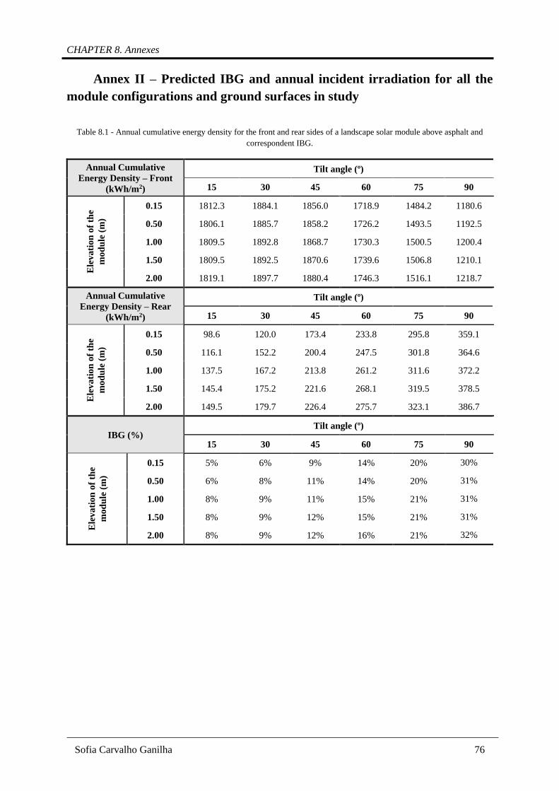
CHAPTER 8. Annexes
Sofia Carvalho Ganilha 76
Annex II – Predicted IBG and annual incident irradiation for all the
module configurations and ground surfaces in study
Table 8.1 - Annual cumulative energy density for the front and rear sides of a landscape solar module above asphalt and
correspondent IBG.
Annual Cumulative
Energy Density – Front
(kWh/m2)
Tilt angle (º)
15 30 45 60 75 90
Ele
va
tio
n o
f th
e
mo
du
le (
m)
0.15 1812.3 1884.1 1856.0 1718.9 1484.2 1180.6
0.50 1806.1 1885.7 1858.2 1726.2 1493.5 1192.5
1.00 1809.5 1892.8 1868.7 1730.3 1500.5 1200.4
1.50 1809.5 1892.5 1870.6 1739.6 1506.8 1210.1
2.00 1819.1 1897.7 1880.4 1746.3 1516.1 1218.7
Annual Cumulative
Energy Density – Rear
(kWh/m2)
Tilt angle (º)
15 30 45 60 75 90
Ele
va
tio
n o
f th
e
mo
du
le (
m)
0.15 98.6 120.0 173.4 233.8 295.8 359.1
0.50 116.1 152.2 200.4 247.5 301.8 364.6
1.00 137.5 167.2 213.8 261.2 311.6 372.2
1.50 145.4 175.2 221.6 268.1 319.5 378.5
2.00 149.5 179.7 226.4 275.7 323.1 386.7
IBG (%) Tilt angle (º)
15 30 45 60 75 90
Ele
va
tio
n o
f th
e
mo
du
le (
m)
0.15 5% 6% 9% 14% 20% 30%
0.50 6% 8% 11% 14% 20% 31%
1.00 8% 9% 11% 15% 21% 31%
1.50 8% 9% 12% 15% 21% 31%
2.00 8% 9% 12% 16% 21% 32%

Potential of bifacial PV installation and its integration with storage solutions
Sofia Carvalho Ganilha 77
Table 8.2 - Annual cumulative energy density for the front and rear sides of a portrait solar module above asphalt and
correspondent IBG.
Annual Cumulative
Energy Density – Front
(kWh/m2)
Tilt angle (º)
15 30 45 60 75 90
Ele
va
tio
n o
f th
e
mo
du
le (
m)
0.15 1808.1 1887.3 1854.6 1722.0 1491.5 1192.7
0.50 1814.7 1890.8 1866.5 1729.4 1496.3 1195.6
1.00 1812.7 1890.7 1869.2 1736.5 1503.6 1207.1
1.50 1817.4 1898.3 1882.2 1744.7 1506.6 1214.8
2.00 1819.9 1897.0 1887.4 1752.6 1520.2 1224.8
Annual Cumulative
Energy Density – Rear
(kWh/m2)
Tilt angle (º)
15 30 45 60 75 90
Ele
va
tion
of
the
mo
du
le (
m)
0.15 96.7 131.8 188.3 241.8 303.4 362.6
0.50 121.7 157.7 205.6 257.2 307.3 368.8
1.00 139.0 170.2 217.4 262.3 316.6 376.9
1.50 146.0 176.5 230.3 272.7 321.8 383.5
2.00 150.2 181.6 232.7 278.7 327.6 390.5
IBG (%) Tilt angle (º)
15 30 45 60 75 90
Ele
va
tio
n o
f th
e
mo
du
le (
m)
0.15 5% 7% 10% 14% 20% 30%
0.50 7% 8% 11% 15% 21% 31%
1.00 8% 9% 12% 15% 21% 31%
1.50 8% 9% 12% 16% 21% 32%
2.00 8% 10% 12% 16% 22% 32%

CHAPTER 8. Annexes
Sofia Carvalho Ganilha 78
Table 8.3 - Annual cumulative energy density for the front and rear sides of a landscape solar module above white painted
concrete and correspondent IBG.
Annual Cumulative
Energy Density – Front
(kWh/m2)
Tilt angle (º)
15 30 45 60 75 90
Ele
va
tio
n o
f th
e
mo
du
le (
m)
0.15 1819.7 1959.3 2018.9 2007.4 1910.0 1764.6
0.50 1822.7 1962.2 2021.0 2005.8 1920.4 1755.6
1.00 1828.9 1962.0 2020.3 2008.7 1919.3 1762.4
1.50 1834.3 1960.5 2021.6 2009.9 1921.5 1766.8
2.00 1827.5 1959.4 2022.6 2008.8 1920.2 1771.2
Annual Cumulative
Energy Density – Rear
(kWh/m2)
Tilt angle (º)
15 30 45 60 75 90
Ele
va
tio
n o
f th
e
mo
du
le (
m)
0.15 687.4 763.8 940.2 884.4 915.7 894.7
0.50 1003.9 1047.1 1048.7 1022.2 974.7 926.5
1.00 1183.4 1168.3 1134.2 1094.3 1030.4 927.3
1.50 1245.4 1219.9 1191.2 1106.2 1026.4 945.8
2.00 1277.0 1274.7 1192.0 1107.5 1042.2 945.9
IBG (%) Tilt angle (º)
15 30 45 60 75 90
Ele
va
tio
n o
f th
e
mo
du
le (
m)
0.15 38% 39% 47% 44% 48% 51%
0.50 55% 53% 52% 51% 51% 53%
1.00 65% 60% 56% 54% 54% 53%
1.50 68% 62% 59% 55% 53% 54%
2.00 70% 65% 59% 55% 54% 53%

Potential of bifacial PV installation and its integration with storage solutions
Sofia Carvalho Ganilha 79
Table 8.4 - Annual cumulative energy density for the front and rear sides of a portrait solar module above white painted
concrete and correspondent IBG.
Annual Cumulative
Energy Density – Front
(kWh/m2)
Tilt angle (º)
15 30 45 60 75 90
Ele
va
tio
n o
f th
e
mo
du
le (
m)
0.15 1830.7 1958.1 2024.0 2006.4 1914.1 1762.5
0.50 1822.8 1955.0 2022.7 2003.8 1915.3 1769.3
1.00 1833.1 1956.3 2024.1 2004.6 1917.3 1770.6
1.50 1820.0 1962.8 2027.2 2012.0 1924.1 1775.3
2.00 1831.1 1957.8 2022.8 2011.1 1920.8 1771.3
Annual Cumulative
Energy Density – Rear
(kWh/m2)
Tilt angle (º)
15 30 45 60 75 90
Ele
va
tion
of
the
mo
du
le (
m)
0.15 871.4 882.0 946.4 959.5 954.3 914.5
0.50 1082.4 1166.6 1142.1 1055.4 999.3 927.4
1.00 1199.2 1186.0 1165.7 1108.1 1032.1 950.4
1.50 1254.1 1232.1 1184.3 1125.8 1037.6 949.8
2.00 1298.9 1246.1 1203.5 1107.8 1047.1 947.0
IBG (%) Tilt angle (º)
15 30 45 60 75 90
Ele
va
tio
n o
f th
e
mo
du
le (
m)
0.15 48% 45% 47% 48% 50% 52%
0.50 59% 60% 56% 53% 52% 52%
1.00 65% 61% 58% 55% 54% 54%
1.50 69% 63% 58% 56% 54% 53%
2.00 71% 64% 59% 55% 55% 53%
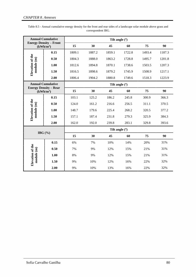
CHAPTER 8. Annexes
Sofia Carvalho Ganilha 80
Table 8.5 - Annual cumulative energy density for the front and rear sides of a landscape solar module above grass and
correspondent IBG.
Annual Cumulative
Energy Density – Front
(kWh/m2)
Tilt angle (º)
15 30 45 60 75 90
Ele
va
tio
n o
f th
e
mo
du
le (
m)
0.15 1809.1 1887.2 1859.1 1722.8 1493.4 1187.3
0.50 1804.3 1888.0 1863.2 1728.8 1495.7 1201.8
1.00 1812.6 1894.8 1870.1 1738.6 1503.5 1207.3
1.50 1816.5 1898.6 1879.2 1745.9 1508.9 1217.1
2.00 1806.4 1904.2 1880.8 1749.6 1518.3 1223.9
Annual Cumulative
Energy Density – Rear
(kWh/m2)
Tilt angle (º)
15 30 45 60 75 90
Ele
va
tio
n o
f th
e
mo
du
le (
m)
0.15 103.1 125.2 186.2 245.8 300.9 366.3
0.50 124.0 161.2 216.6 256.5 311.1 370.5
1.00 148.7 179.6 225.4 268.2 320.5 377.2
1.50 157.1 187.4 231.8 279.3 325.9 384.3
2.00 162.0 192.0 239.8 283.1 329.8 393.6
IBG (%) Tilt angle (º)
15 30 45 60 75 90
Ele
va
tio
n o
f th
e
mo
du
le (
m)
0.15 6% 7% 10% 14% 20% 31%
0.50 7% 9% 12% 15% 21% 31%
1.00 8% 9% 12% 15% 21% 31%
1.50 9% 10% 12% 16% 22% 32%
2.00 9% 10% 13% 16% 22% 32%
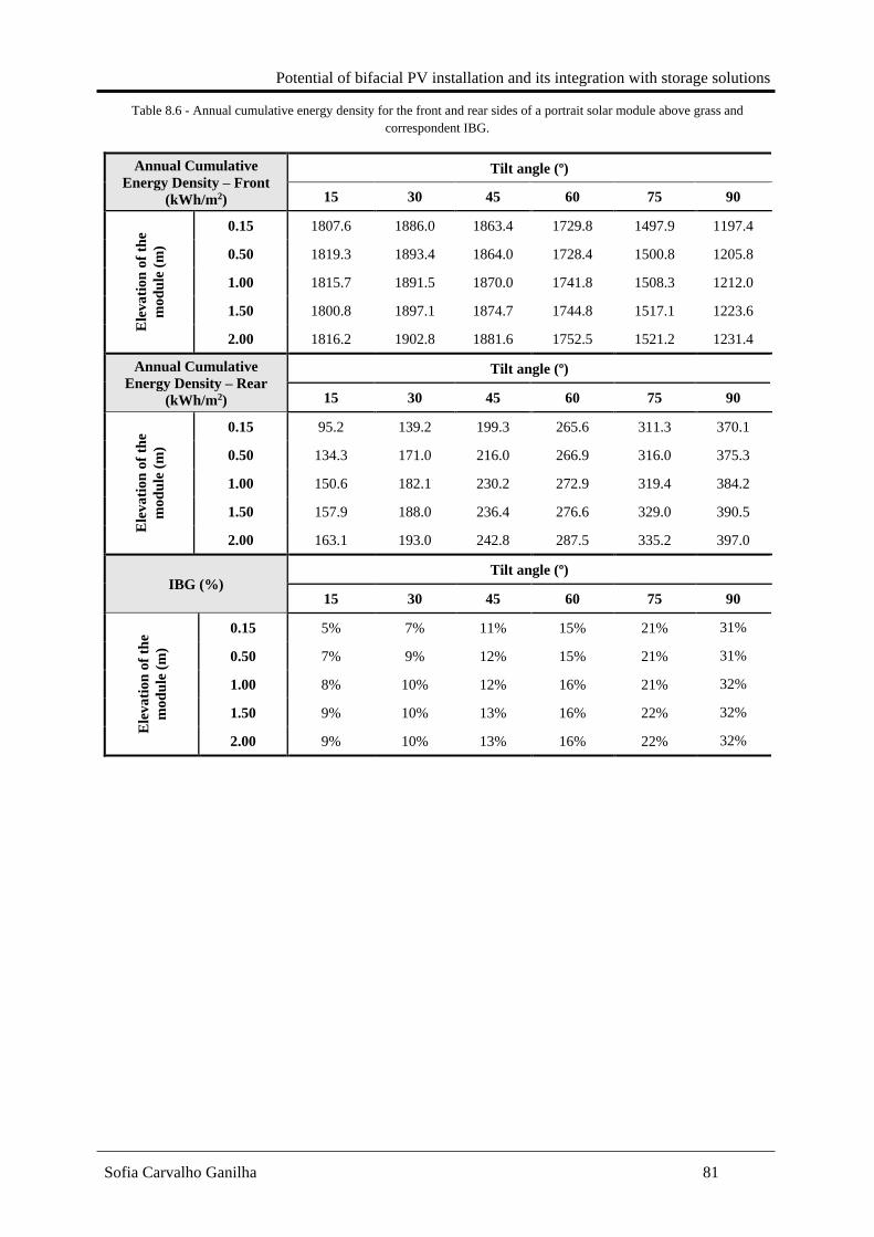
Potential of bifacial PV installation and its integration with storage solutions
Sofia Carvalho Ganilha 81
Table 8.6 - Annual cumulative energy density for the front and rear sides of a portrait solar module above grass and
correspondent IBG.
Annual Cumulative
Energy Density – Front
(kWh/m2)
Tilt angle (º)
15 30 45 60 75 90
Ele
va
tio
n o
f th
e
mo
du
le (
m)
0.15 1807.6 1886.0 1863.4 1729.8 1497.9 1197.4
0.50 1819.3 1893.4 1864.0 1728.4 1500.8 1205.8
1.00 1815.7 1891.5 1870.0 1741.8 1508.3 1212.0
1.50 1800.8 1897.1 1874.7 1744.8 1517.1 1223.6
2.00 1816.2 1902.8 1881.6 1752.5 1521.2 1231.4
Annual Cumulative
Energy Density – Rear
(kWh/m2)
Tilt angle (º)
15 30 45 60 75 90
Ele
va
tion
of
the
mo
du
le (
m)
0.15 95.2 139.2 199.3 265.6 311.3 370.1
0.50 134.3 171.0 216.0 266.9 316.0 375.3
1.00 150.6 182.1 230.2 272.9 319.4 384.2
1.50 157.9 188.0 236.4 276.6 329.0 390.5
2.00 163.1 193.0 242.8 287.5 335.2 397.0
IBG (%) Tilt angle (º)
15 30 45 60 75 90
Ele
va
tio
n o
f th
e
mo
du
le (
m)
0.15 5% 7% 11% 15% 21% 31%
0.50 7% 9% 12% 15% 21% 31%
1.00 8% 10% 12% 16% 21% 32%
1.50 9% 10% 13% 16% 22% 32%
2.00 9% 10% 13% 16% 22% 32%
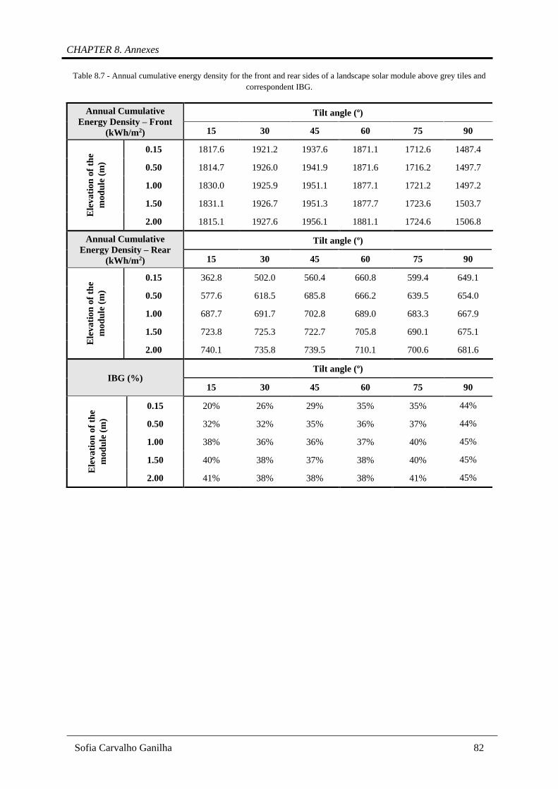
CHAPTER 8. Annexes
Sofia Carvalho Ganilha 82
Table 8.7 - Annual cumulative energy density for the front and rear sides of a landscape solar module above grey tiles and
correspondent IBG.
Annual Cumulative
Energy Density – Front
(kWh/m2)
Tilt angle (º)
15 30 45 60 75 90
Ele
va
tio
n o
f th
e
mo
du
le (
m)
0.15 1817.6 1921.2 1937.6 1871.1 1712.6 1487.4
0.50 1814.7 1926.0 1941.9 1871.6 1716.2 1497.7
1.00 1830.0 1925.9 1951.1 1877.1 1721.2 1497.2
1.50 1831.1 1926.7 1951.3 1877.7 1723.6 1503.7
2.00 1815.1 1927.6 1956.1 1881.1 1724.6 1506.8
Annual Cumulative
Energy Density – Rear
(kWh/m2)
Tilt angle (º)
15 30 45 60 75 90
Ele
va
tio
n o
f th
e
mo
du
le (
m)
0.15 362.8 502.0 560.4 660.8 599.4 649.1
0.50 577.6 618.5 685.8 666.2 639.5 654.0
1.00 687.7 691.7 702.8 689.0 683.3 667.9
1.50 723.8 725.3 722.7 705.8 690.1 675.1
2.00 740.1 735.8 739.5 710.1 700.6 681.6
IBG (%) Tilt angle (º)
15 30 45 60 75 90
Ele
va
tio
n o
f th
e
mo
du
le (
m)
0.15 20% 26% 29% 35% 35% 44%
0.50 32% 32% 35% 36% 37% 44%
1.00 38% 36% 36% 37% 40% 45%
1.50 40% 38% 37% 38% 40% 45%
2.00 41% 38% 38% 38% 41% 45%
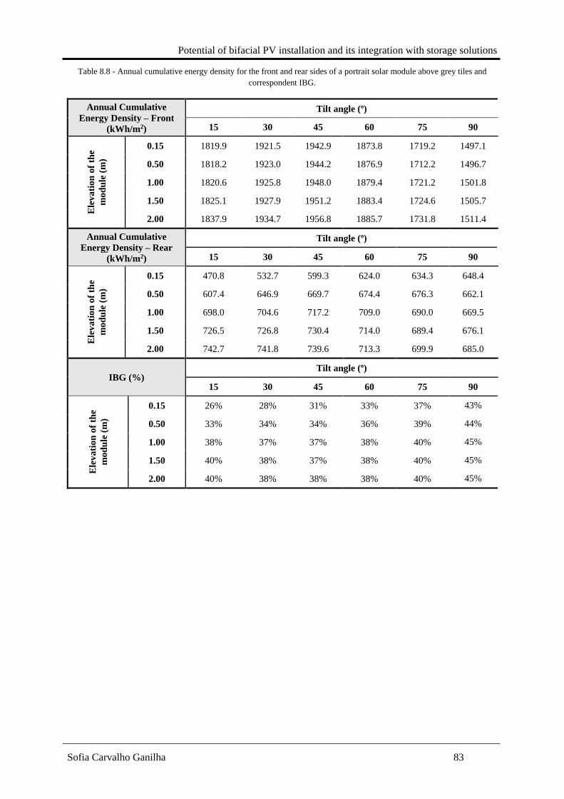
Potential of bifacial PV installation and its integration with storage solutions
Sofia Carvalho Ganilha 83
Table 8.8 - Annual cumulative energy density for the front and rear sides of a portrait solar module above grey tiles and
correspondent IBG.
Annual Cumulative
Energy Density – Front
(kWh/m2)
Tilt angle (º)
15 30 45 60 75 90
Ele
va
tio
n o
f th
e
mo
du
le (
m)
0.15 1819.9 1921.5 1942.9 1873.8 1719.2 1497.1
0.50 1818.2 1923.0 1944.2 1876.9 1712.2 1496.7
1.00 1820.6 1925.8 1948.0 1879.4 1721.2 1501.8
1.50 1825.1 1927.9 1951.2 1883.4 1724.6 1505.7
2.00 1837.9 1934.7 1956.8 1885.7 1731.8 1511.4
Annual Cumulative
Energy Density – Rear
(kWh/m2)
Tilt angle (º)
15 30 45 60 75 90
Ele
va
tion
of
the
mo
du
le (
m)
0.15 470.8 532.7 599.3 624.0 634.3 648.4
0.50 607.4 646.9 669.7 674.4 676.3 662.1
1.00 698.0 704.6 717.2 709.0 690.0 669.5
1.50 726.5 726.8 730.4 714.0 689.4 676.1
2.00 742.7 741.8 739.6 713.3 699.9 685.0
IBG (%) Tilt angle (º)
15 30 45 60 75 90
Ele
va
tio
n o
f th
e
mo
du
le (
m)
0.15 26% 28% 31% 33% 37% 43%
0.50 33% 34% 34% 36% 39% 44%
1.00 38% 37% 37% 38% 40% 45%
1.50 40% 38% 37% 38% 40% 45%
2.00 40% 38% 38% 38% 40% 45%

CHAPTER 8. Annexes
Sofia Carvalho Ganilha 84
Table 8.9 - Annual cumulative energy density for the front and rear sides of a landscape solar module above white gravel and
correspondent IBG.
Annual Cumulative
Energy Density – Front
(kWh/m2)
Tilt angle (º)
15 30 45 60 75 90
Ele
va
tio
n o
f th
e
mo
du
le (
m)
0.15 1816.6 1919.0 1945.1 1876.3 1721.6 1508.3
0.50 1818.9 1921.7 1948.9 1883.3 1724.2 1509.9
1.00 1822.7 1928.1 1951.6 1882.2 1723.6 1512.3
1.50 1820.3 1931.2 1957.5 1885.6 1731.7 1517.0
2.00 1832.8 1935.2 1956.3 1890.8 1736.6 1517.5
Annual Cumulative
Energy Density – Rear
(kWh/m2)
Tilt angle (º)
15 30 45 60 75 90
Ele
va
tio
n o
f th
e
mo
du
le (
m)
0.15 555.3 355.4 491.4 526.6 576.1 657.2
0.50 550.0 589.4 627.6 657.7 673.2 690.5
1.00 702.9 712.3 718.3 727.1 719.4 704.1
1.50 757.1 752.2 755.5 756.4 724.4 718.0
2.00 772.0 772.3 775.2 768.8 736.8 714.6
IBG (%) Tilt angle (º)
15 30 45 60 75 90
Ele
va
tio
n o
f th
e
mo
du
le (
m)
0.15 20% 26% 27% 31% 38% 42%
0.50 32% 33% 34% 36% 40% 44%
1.00 39% 37% 37% 38% 41% 45%
1.50 41% 39% 39% 38% 41% 45%
2.00 42% 40% 39% 39% 41% 46%

Potential of bifacial PV installation and its integration with storage solutions
Sofia Carvalho Ganilha 85
Table 8.10 - Annual cumulative energy density for the front and rear sides of a portrait solar module above white gravel and
correspondent IBG.
Annual Cumulative
Energy Density – Front
(kWh/m2)
Tilt angle (º)
15 30 45 60 75 90
Ele
va
tio
n o
f th
e
mo
du
le (
m)
0.15 1817.4 1923.7 1949.1 1880.6 1724.0 1507.8
0.50 1811.7 1926.5 1950.8 1884.4 1725.6 1508.9
1.00 1821.7 1925.4 1953.4 1882.5 1730.7 1517.1
1.50 1823.5 1937.0 1959.2 1887.9 1734.2 1524.3
2.00 1817.7 1933.9 1962.8 1892.8 1733.5 1525.7
Annual Cumulative
Energy Density – Rear
(kWh/m2)
Tilt angle (º)
15 30 45 60 75 90
Ele
va
tion
of
the
mo
du
le (
m)
0.15 428.4 578.6 631.8 639.8 650.4 664.9
0.50 639.1 689.4 729.7 703.5 674.2 674.3
1.00 722.0 735.8 752.1 734.0 701.2 688.5
1.50 756.8 758.1 764.4 719.9 718.2 694.0
2.00 773.0 773.2 773.4 743.3 720.2 698.7
IBG (%) Tilt angle (º)
15 30 45 60 75 90
Ele
va
tio
n o
f th
e
mo
du
le (
m)
0.15 24% 30% 32% 34% 38% 44%
0.50 35% 36% 37% 37% 39% 45%
1.00 40% 38% 39% 39% 41% 45%
1.50 42% 39% 39% 38% 41% 46%
2.00 43% 40% 39% 39% 42% 46%

CHAPTER 8. Annexes
Sofia Carvalho Ganilha 86
Annex III - PrismSolar® MODEL Bi60-343BSTC

Potential of bifacial PV installation and its integration with storage solutions
Sofia Carvalho Ganilha 87
Annex IV – Predicted energy yield for all the module configurations in
study
Table 8.11 - Annual energy converted normalized by the area of the module - Energy Yield (kWh/m2) - or by the peak power
- Specific Yield (kWh/kWp) -, for all the module configurations considered in the electrical model.
Technology Orientation Mounting
Position
Tilt angle
(º)
Energy Yield
(kWh/m2)
Specific Yield
(kWh/kWp)
Monofacial South Landscape 15 309.57 1536.40
Bifacial South Landscape 15 403.74 1577.28
Monofacial South Landscape 30 326.86 1622.22
Bifacial South Landscape 30 420.77 1643.82
Bifacial South Portrait 30 420.53 1642.88
Monofacial South Landscape 45 329.38 1634.70
Bifacial South Landscape 45 422.26 1649.65
Monofacial South Landscape 60 317.10 1573.75
Bifacial South Landscape 60 408.72 1596.75
Monofacial South Landscape 75 290.78 1443.15
Bifacial South Landscape 75 380.67 1487.15
Monofacial South Landscape 90 252.90 1255.12
Bifacial South Landscape 90 336.66 1315.25
Bifacial East Portrait 90 370.29 1446.61
Bifacial West Portrait 90 364.96 1425.79
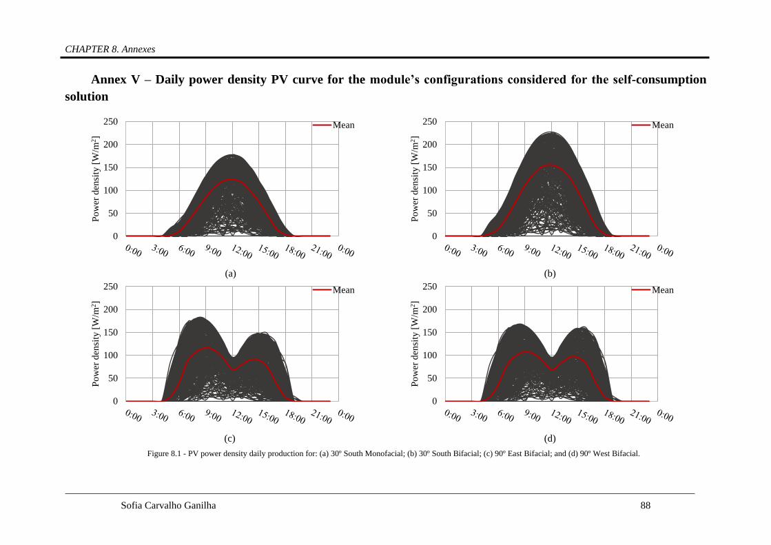
CHAPTER 8. Annexes
Sofia Carvalho Ganilha 88
Annex V – Daily power density PV curve for the module’s configurations considered for the self-consumption
solution
Figure 8.1 - PV power density daily production for: (a) 30º South Monofacial; (b) 30º South Bifacial; (c) 90º East Bifacial; and (d) 90º West Bifacial.
0
50
100
150
200
250
Pow
er d
ensi
ty [
W/m
2]
Mean
0
50
100
150
200
250
Pow
er d
ensi
ty [
W/m
2]
Mean
0
50
100
150
200
250
Pow
er d
ensi
ty [
W/m
2]
Mean
0
50
100
150
200
250
Pow
er d
ensi
ty [
W/m
2]
Mean
(b)
(c)
(d)
(a)

Potential of bifacial PV installation and its integration with storage solutions
Sofia Carvalho Ganilha 89
Annex VI – SSR and SCR for the module configurations and battery
capacities in study
Table 8.12 - SSR for a self-consumption system depending on the storage capacity and the configuration and area of the
modules installed.
PV
installation
area (m2)
Technology Orientation Tilt angle
(º)
Battery Capacity (kWh/kWp)
0 0.5 1.0 1.5 2.0
1.34
Monofacial South 30 15% 15% 15% 15% 15%
Bifacial South 30 20% 20% 20% 20% 20%
Bifacial East 90 17% 17% 17% 17% 17%
Bifacial West 90 17% 17% 17% 17% 17%
2.68
Monofacial South 30 28% 28% 28% 30% 30%
Bifacial South 30 32% 32% 32% 37% 38%
Bifacial East 90 31% 32% 31% 34% 34%
Bifacial West 90 31% 32% 31% 33% 34%
4.02
Monofacial South 30 34% 35% 39% 41% 43%
Bifacial South 30 37% 39% 44% 48% 50%
Bifacial East 90 38% 39% 44% 46% 48%
Bifacial West 90 38% 39% 43% 46% 48%
5.36
Monofacial South 30 37% 39% 45% 49% 52%
Bifacial South 30 39% 45% 51% 56% 60%
Bifacial East 90 41% 46% 51% 55% 58%
Bifacial West 90 41% 46% 51% 55% 58%
6.70
Monofacial South 30 39% 44% 50% 55% 60%
Bifacial South 30 41% 48% 56% 62% 69%
Bifacial East 90 43% 50% 57% 63% 67%
Bifacial West 90 43% 50% 57% 62% 67%
8.04
Monofacial South 30 40% 47% 54% 60% 66%
Bifacial South 30 42% 51% 60% 69% 76%
Bifacial East 90 44% 53% 62% 69% 75%
Bifacial West 90 44% 53% 62% 69% 75%

CHAPTER 8. Annexes
Sofia Carvalho Ganilha 90
Table 8.13 - SCR for a self-consumption system depending on the storage capacity and the configuration and area of the
modules installed.
PV
installation
area (m2)
Technology Orientation Tilt angle
(º)
Battery Capacity (kWh/kWp)
0 0.5 1.0 1.5 2.0
1.34
Monofacial South 30 100% 100% 100% 100% 100%
Bifacial South 30 100% 100% 100% 100% 100%
Bifacial East 90 100% 100% 100% 100% 100%
Bifacial West 90 100% 100% 100% 100% 100%
2.68
Monofacial South 30 92% 96% 98% 100% 100%
Bifacial South 30 82% 87% 91% 94% 97%
Bifacial East 90 91% 96% 99% 99% 100%
Bifacial West 90 92% 97% 99% 100% 100%
4.02
Monofacial South 30 74% 81% 86% 90% 94%
Bifacial South 30 63% 70% 76% 81% 86%
Bifacial East 90 74% 81% 85% 90% 93%
Bifacial West 90 75% 82% 86% 90% 94%
5.36
Monofacial South 30 61% 68% 75% 81% 86%
Bifacial South 30 51% 58% 65% 71% 77%
Bifacial East 90 60% 68% 75% 80% 85%
Bifacial West 90 61% 69% 75% 81% 85%
6.70
Monofacial South 30 51% 59% 66% 73% 79%
Bifacial South 30 42% 50% 57% 64% 70%
Bifacial East 90 50% 59% 66% 73% 78%
Bifacial West 90 51% 60% 67% 74% 79%
8.04
Monofacial South 30 45% 52% 60% 67% 73%
Bifacial South 30 36% 44% 52% 59% 65%
Bifacial East 90 43% 52% 60% 67% 73%
Bifacial West 90 44% 53% 61% 68% 74%


![Simplified Robust Control Design Method F Wide Area ... · Regulador Linear Quadrático assim como em [9]. Esse ... Nas simulações não-lineares (seção VII.C) os atrasos foram](https://img.pdfslide.us/doc/110x75/5ba8a5f409d3f2592c8c8669/simplified-robust-control-design-method-f-wide-area-regulador-linear-quadratico.jpg)