Potential for radio occultation to identify/correct other satellite observation biases

Sean Healy

Outline• Describe the GPS radio occultation measurement technique and

outline the processing of the raw observations. Outline strengths weaknesses.

• Show comparisons from different processing centres (Wickert et al).

• Describe the forward problem and summarise forecast impact experiments where GPS RO bending angles have been assimilated without bias correction and have partially corrected known model problems.

• Implications for identifying/correcting biases in other observations.

• Summary.

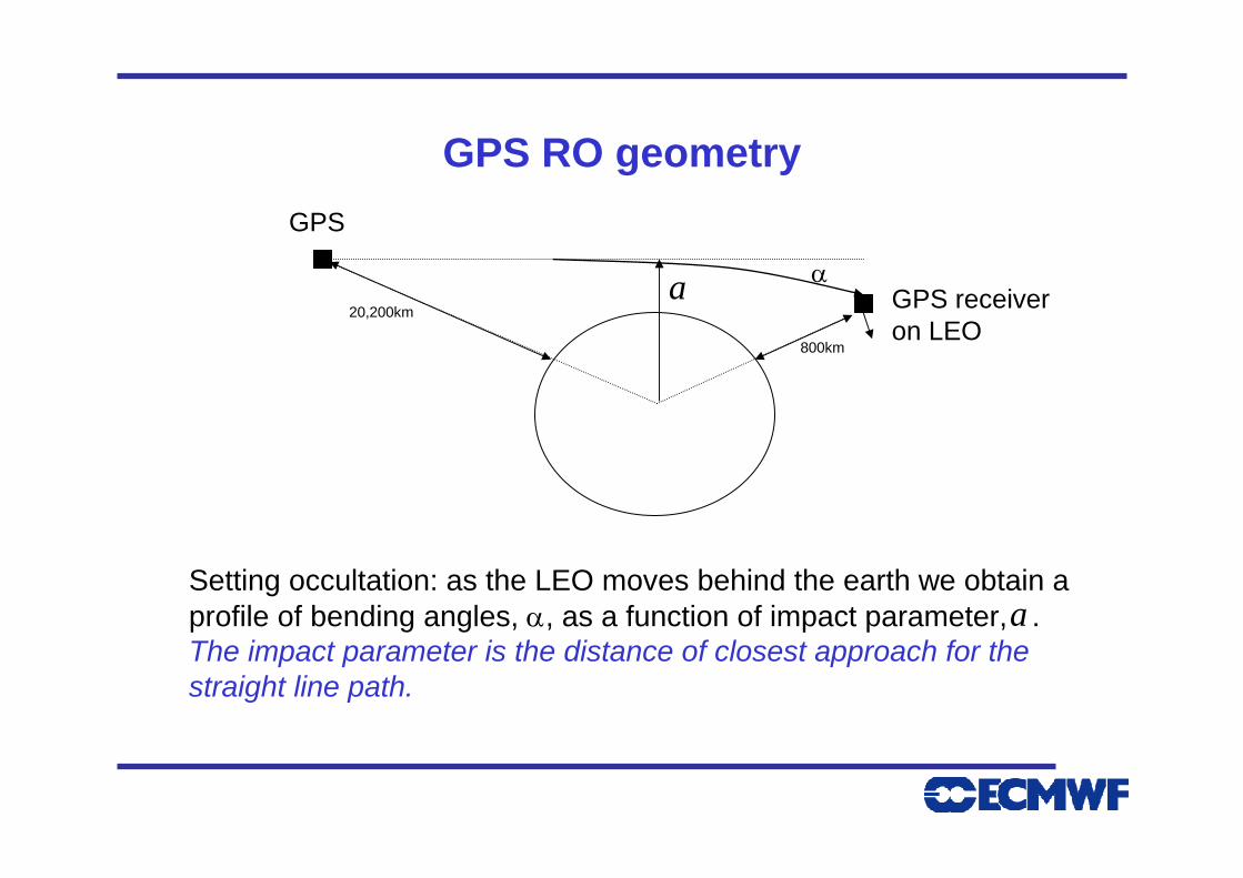
GPS RO geometryGPS

GPS receiveron LEO

α

Setting occultation: as the LEO moves behind the earth we obtain a profile of bending angles, α, as a function of impact parameter, . The impact parameter is the distance of closest approach for thestraight line path.

20,200km

800km

a

a

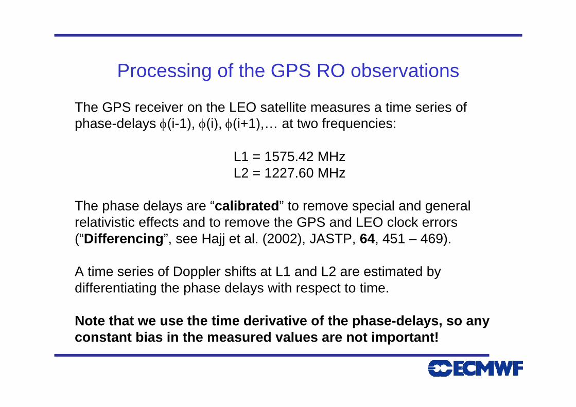
Processing of the GPS RO observations

The GPS receiver on the LEO satellite measures a time series of phase-delays φ(i-1), φ(i), φ(i+1),… at two frequencies:

L1 = 1575.42 MHzL2 = 1227.60 MHz

The phase delays are “calibrated” to remove special and general relativistic effects and to remove the GPS and LEO clock errors (“Differencing”, see Hajj et al. (2002), JASTP, 64, 451 – 469).

A time series of Doppler shifts at L1 and L2 are estimated by differentiating the phase delays with respect to time.

Note that we use the time derivative of the phase-delays, so any constant bias in the measured values are not important!

Processing of the GPS RO observations (2)

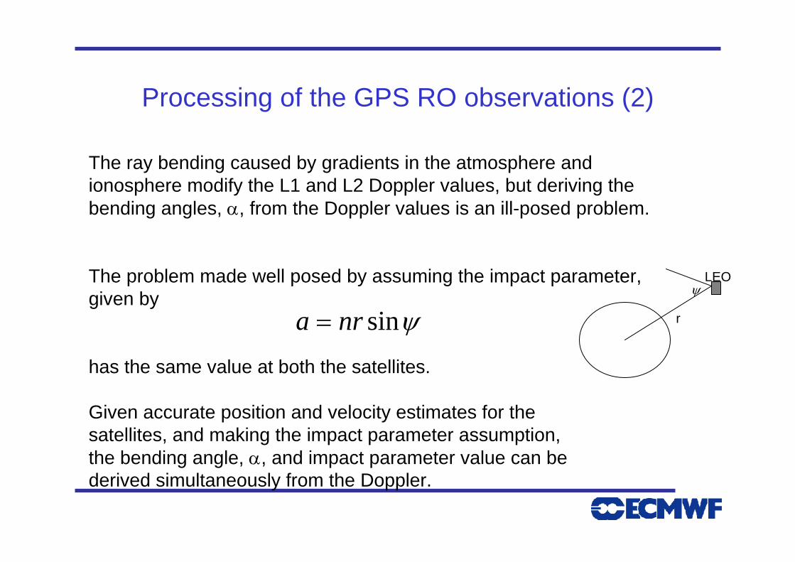
The ray bending caused by gradients in the atmosphere and ionosphere modify the L1 and L2 Doppler values, but deriving thebending angles, α, from the Doppler values is an ill-posed problem.

The problem made well posed by assuming the impact parameter, given by

has the same value at both the satellites.

Given accurate position and velocity estimates for thesatellites, and making the impact parameter assumption,the bending angle, α, and impact parameter value can bederived simultaneously from the Doppler.

LEOψ

rψsinnra =

The ionospheric correction

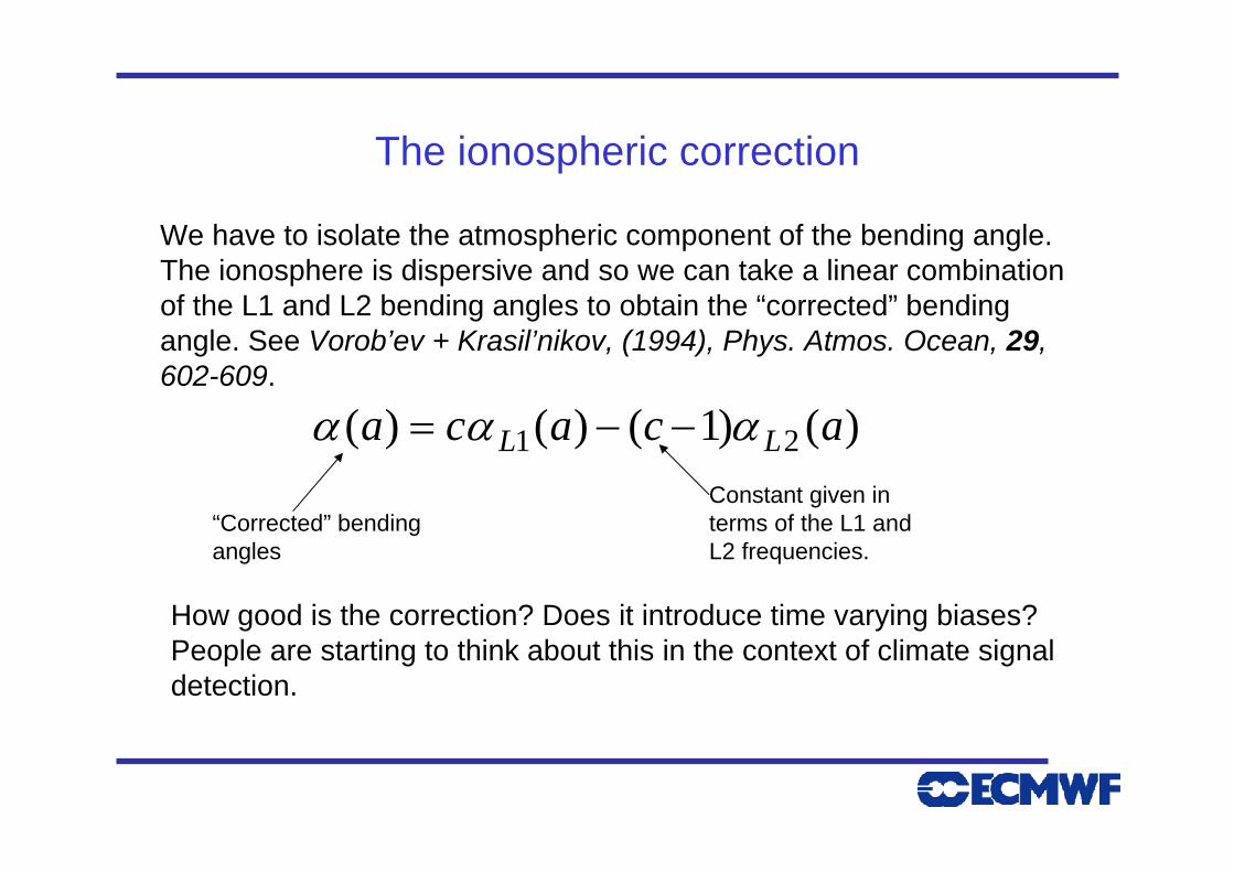
We have to isolate the atmospheric component of the bending angle. The ionosphere is dispersive and so we can take a linear combination of the L1 and L2 bending angles to obtain the “corrected” bending angle. See Vorob’ev + Krasil’nikov, (1994), Phys. Atmos. Ocean, 29, 602-609.

)()1()()( 21 acaca LL ααα −−=

“Corrected” bendingangles

Constant given in terms of the L1 and L2 frequencies.

How good is the correction? Does it introduce time varying biases? People are starting to think about this in the context of climate signal detection.

The ionospheric correction: A simulated example

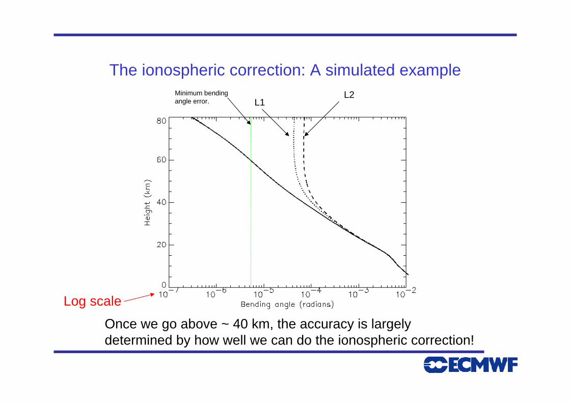
L1L2

Once we go above ~ 40 km, the accuracy is largely determined by how well we can do the ionospheric correction!

Minimum bendingangle error.

Log scale

Deriving the refractive index profiles

∫∞

−−=

a

dxaxdx

ndaa

22

ln2)(α

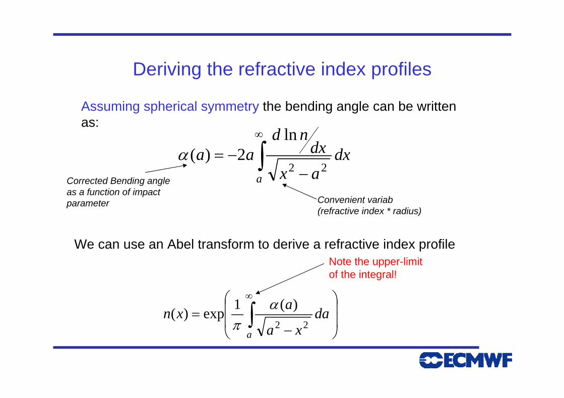
Assuming spherical symmetry the bending angle can be written as:

We can use an Abel transform to derive a refractive index profile

Convenient variab(refractive index * radius)

Corrected Bending angle as a function of impactparameter

⎟⎟

⎠

⎞

⎜⎜

⎝

⎛

−= ∫

∞

a

daxa

axn22

)(1exp)( απ

Note the upper-limitof the integral!

Refractivity and Pressure/temperature profiles:“Classical retrieval”

221

6 )1(10

TPc

TPc

nN

w+=

−= −

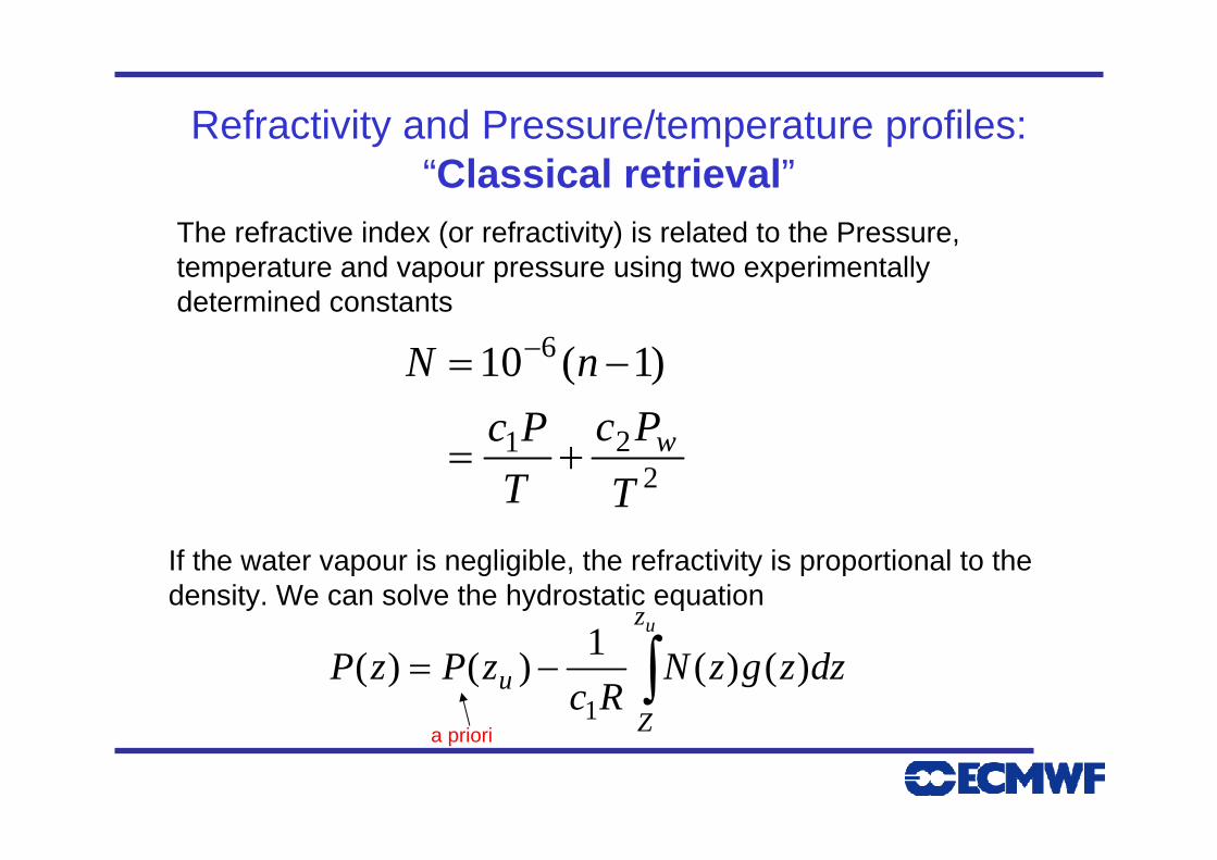
The refractive index (or refractivity) is related to the Pressure, temperature and vapour pressure using two experimentally determined constants

If the water vapour is negligible, the refractivity is proportional to the density. We can solve the hydrostatic equation

∫−=uz

Zu dzzgzN

RczPzP )()(1)()(

1a priori

Limitations (1)

In order to derive refractivity the (noisy) bending angle profiles must be extrapolated to infinity – i.e., we have to introduce a-priori. This blending of the observed and simulated bending angles is called “statistical optimisation”. The refractivity profiles above ~35 km are sensitive to the choice of a priori.

The temperature profiles require a-priori information to initialise the hydrostatic integration. Sometimes ECMWF temperature at 40km!

I would be sceptical about any GPSRO temperature profile above ~30-35 km, derived with the classical approach. It will be very sensitive to the a-priori!

Limitations(2)

The refractivity profiles in the lower troposphere are biased low when compared to NWP models, particularly in the tropics. See Ao et al JGR, (2003), 108, doi10.1029/2002JD003216.

This is an area of on-going research:

•Multipath processing – more than one ray is measured by the receiver (Full Spectral Inversion).

•Improved receiver software (Open-loop processing).

But there are also physical limitations: “ducting regions”. If the vertical refractive index gradient exceeds a critical value, thesignal is lost.

eRdrdn 1≥−

ROSE: Comparison of CHAMP RO analysis results from GFZ, UCAR

and JPL

J. Wickert, C.O. Ao, W.B. Schreinerand the GFZ, JPL, and UCAR analysis teams

CHAMP occultation dataprovision and analysis at GFZ, JPL & UCARThe question is:Are the resultscomparable?

Wickert et al.

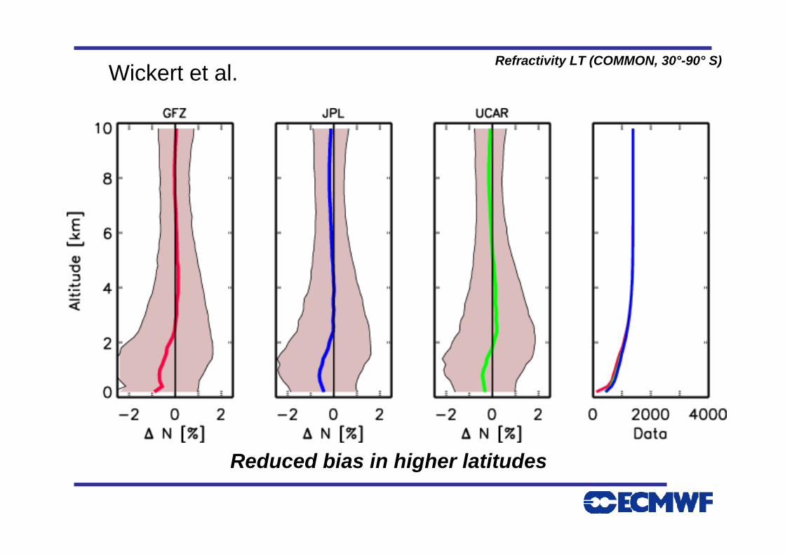
Refractivity LT (COMMON, 30°-90° S)

Reduced bias in higher latitudes

Wickert et al.

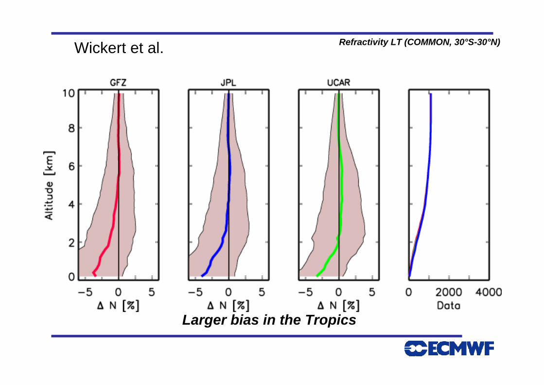
Refractivity LT (COMMON, 30°S-30°N)

Larger bias in the Tropics

Wickert et al.

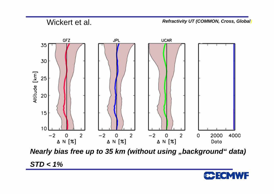
Refractivity UT (COMMON, Cross, Global)

Nearly bias free up to 35 km (without using „background“ data)

STD < 1%

Wickert et al.

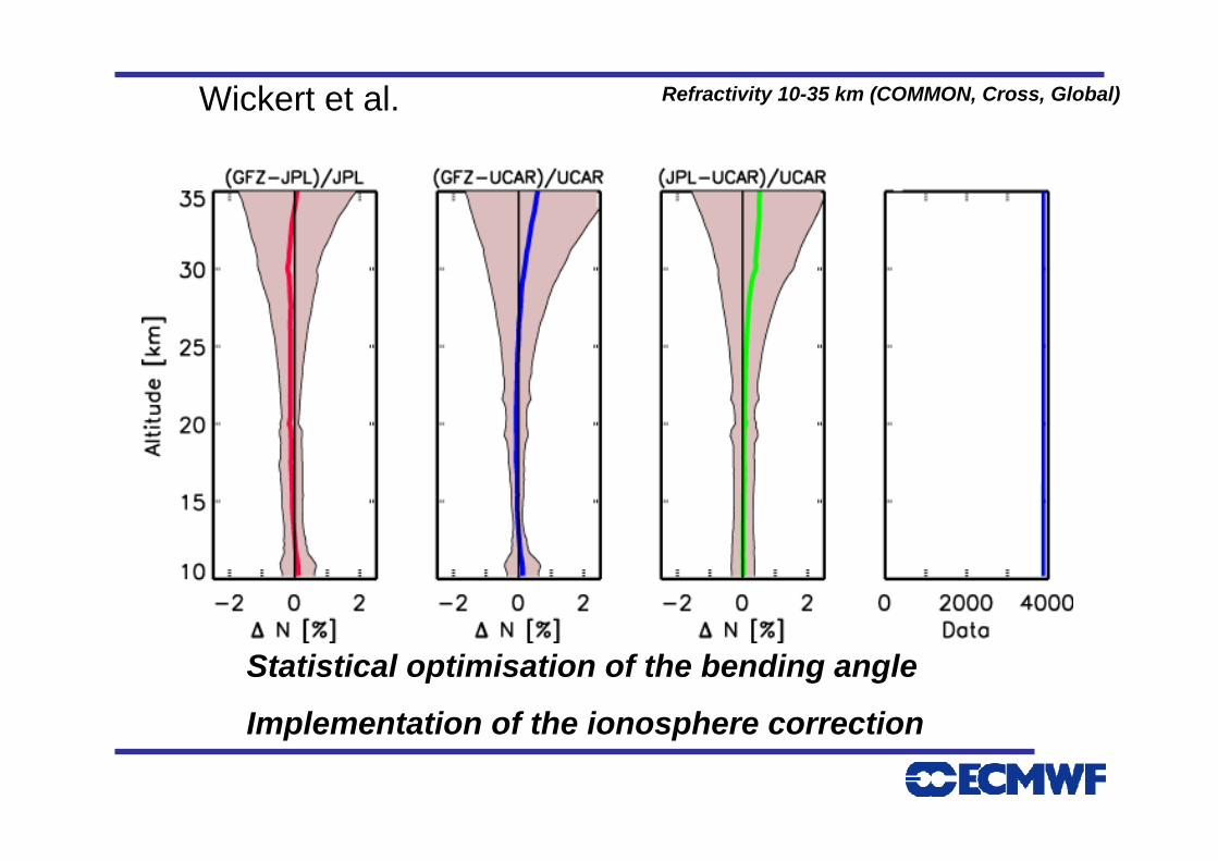
Refractivity 10-35 km (COMMON, Cross, Global)

Statistical optimisation of the bending angle

Implementation of the ionosphere correction

Wickert et al.

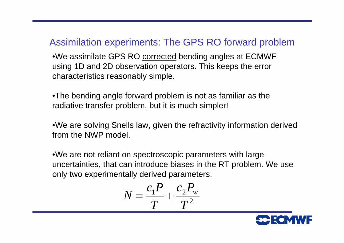
Assimilation experiments: The GPS RO forward problem •We assimilate GPS RO corrected bending angles at ECMWF using 1D and 2D observation operators. This keeps the error characteristics reasonably simple.

•The bending angle forward problem is not as familiar as the radiative transfer problem, but it is much simpler!

•We are solving Snells law, given the refractivity information derived from the NWP model.

•We are not reliant on spectroscopic parameters with large uncertainties, that can introduce biases in the RT problem. We use only two experimentally derived parameters.

221

TPc

TPcN w+=

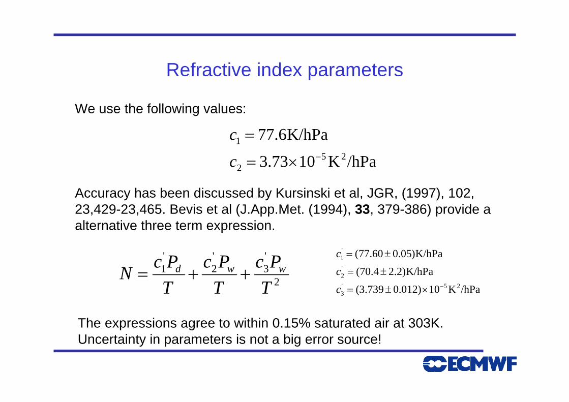
Refractive index parameters

/hPaK1073.3

K/hPa6.7725

2

1−×=

=

c

c

2

'3

'2

'1

TPc

TPc

TPcN wwd ++=

We use the following values:

Accuracy has been discussed by Kursinski et al, JGR, (1997), 102, 23,429-23,465. Bevis et al (J.App.Met. (1994), 33, 379-386) provide a alternative three term expression.

/hPaK10)012.0739.3(

K/hPa)2.24.70(

K/hPa)05.060.77(

25'3

'2

'1

−×±=

±=

±=

c

c

c

The expressions agree to within 0.15% saturated air at 303K. Uncertainty in parameters is not a big error source!

Assimilation experiments

• We have run forecast experiments assimilating CHAMP radio occultation measurements from June 1st – 31st July, 2004, in addition to the observation that are assimilated operationally.

• We can assimilate the CHAMP ionospheric corrected bending angles with 1D and 2D observation, but only the 1D results are presented here.

• CHAMP provides around 80 profiles per 12 hour assimilation window. This gives a total of ~12500 bending angles. We use the data processed at UCAR, with tangent heights up to 40km.

• The bending angles are assimilated without bias correction.

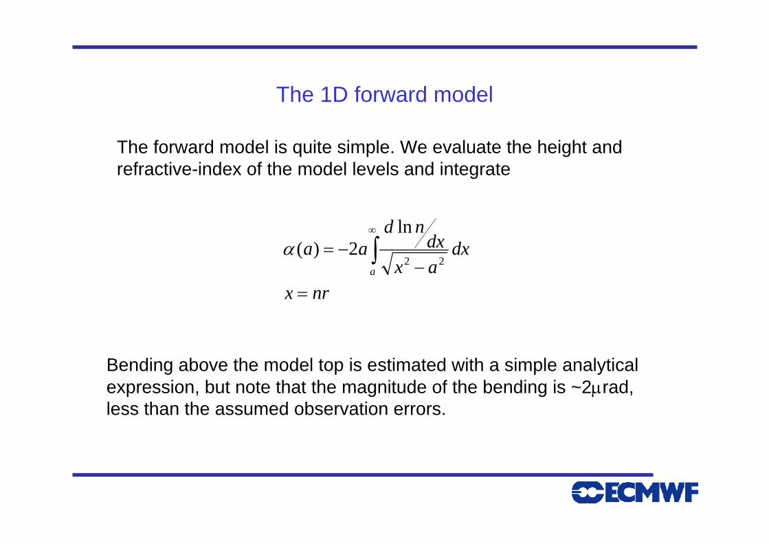
The 1D forward model

The forward model is quite simple. We evaluate the height and refractive-index of the model levels and integrate

nrx

dxaxdx

ndaa

a

=−

−= ∫∞

22

ln2)(α

Bending above the model top is estimated with a simple analytical expression, but note that the magnitude of the bending is ~2µrad, less than the assumed observation errors.

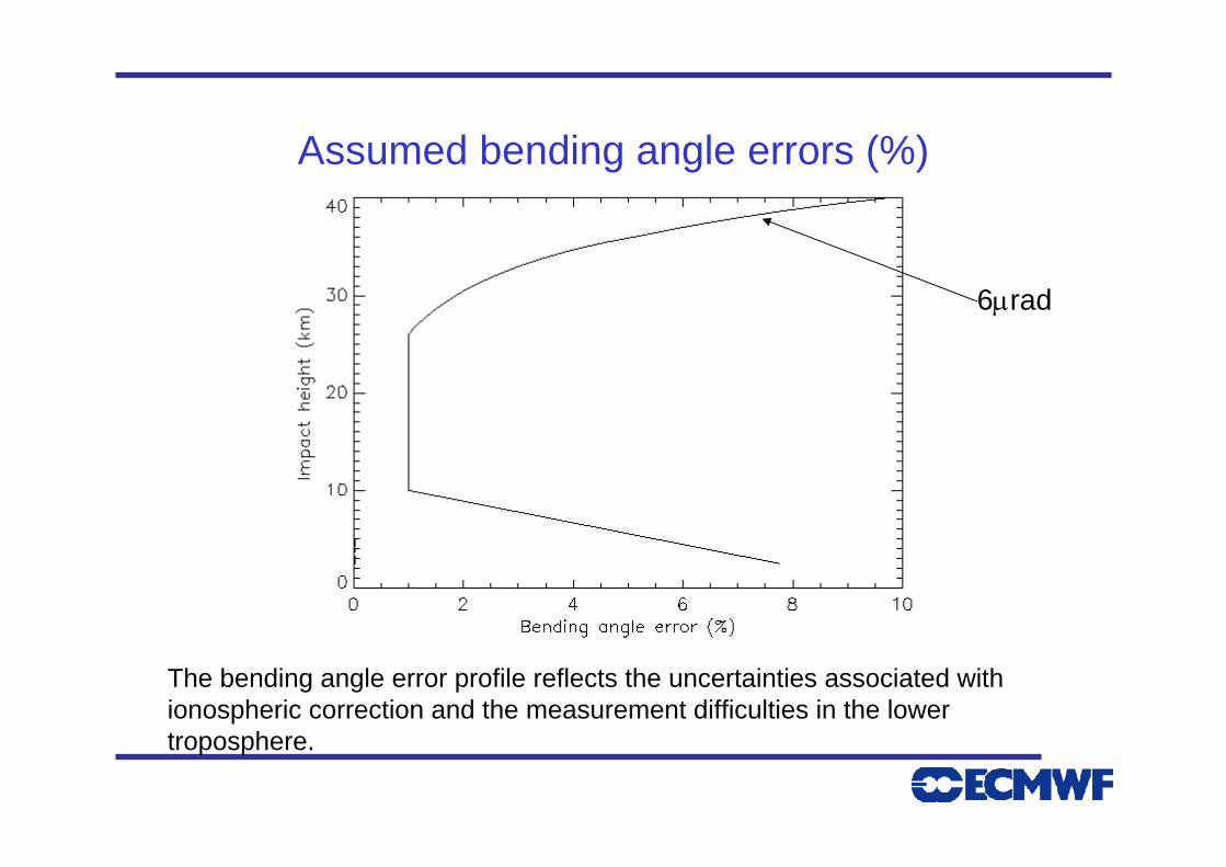
Assumed bending angle errors (%)

The bending angle error profile reflects the uncertainties associated with ionospheric correction and the measurement difficulties in the lower troposphere.

6µrad

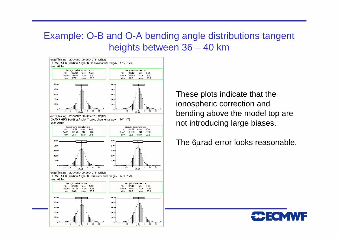
Example: O-B and O-A bending angle distributions tangent heights between 36 – 40 km

These plots indicate that the ionospheric correction and bending above the model top are not introducing large biases.

The 6µrad error looks reasonable.

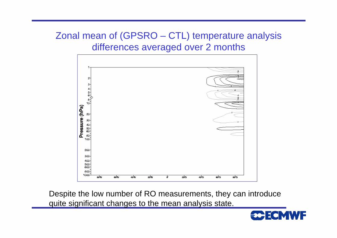
Zonal mean of (GPSRO – CTL) temperature analysis differences averaged over 2 months

Despite the low number of RO measurements, they can introduce quite significant changes to the mean analysis state.

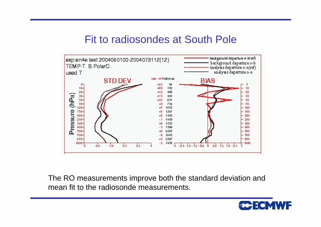
Fit to radiosondes at South Pole

The RO measurements improve both the standard deviation and mean fit to the radiosonde measurements.

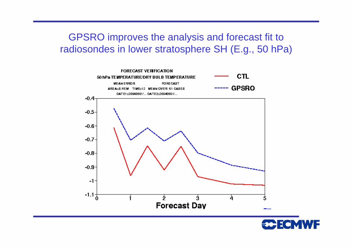
GPSRO improves the analysis and forecast fit to radiosondes in lower stratosphere SH (E.g., 50 hPa)

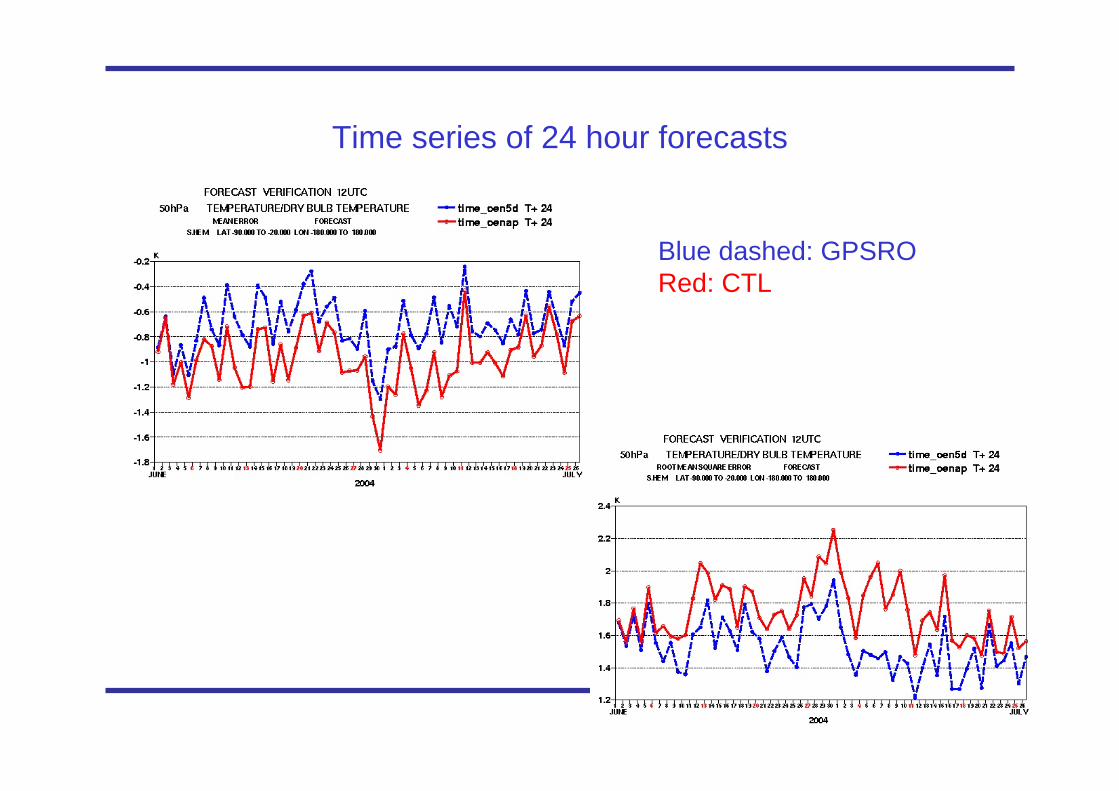
Time series of 24 hour forecasts

Blue dashed: GPSRORed: CTL

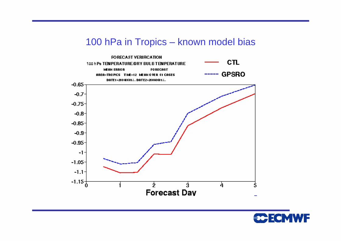
100 hPa in Tropics – known model bias

Implications for bias correction of other measurements

• We have not observed any significant changes in the radiance bias statistics as a result of assimilating the GPS RO measurements in these experiments.

• The radiance measurements are bias corrected against the model. It is hoped that the assimilation of radiosondes prevents the model from drifting, so the radiances are indirectly “tied” to the radiosondes.

• The CHAMP GPS RO measurements have improved the fit to radiosondesin regions where there are known model problems.

• We expect to obtain GRAS and COSMIC measurements next year – almost an order of magnitude more data.

• GRAS and COSMIC data should improve the temperature analyses in the upper-troposphere and lower-stratosphere. The measurements should help distinguish between model and observation biases.

Summary

• Raw GPS RO measurements are based on the time derivative of a measured phase delay. However, a number of pre-processing steps are required to derive the bending angle and refractivity profiles that are assimilated. These steps will introduce a-priori and limit the height range of which the measurements are accurate. E.g., we won’t correct errors at the stratopause with GPS RO.

• The GPS RO information content is highest in the ~10 – 30 km height region.

• The GPS RO forward problem is relatively simple. The refractive index parameters are well known and do not introduce large biases. Errors less than 0.15%.

Summary (2)

• We have performed a 2 month forecast impact experiment and assimilated CHAMP GPS RO corrected bending angles without bias correction.

• Assimilating the measurements has improved the fit to radiosondemeasurements in regions where there are known model problems (S.Pole, 100hPa in the tropics).

• GRAS and COSMIC GPS RO measurements will be available from 2006. The measurements should improve the temperature analyses in the upper-troposphere and lower-stratosphere.

• This will help distinguish between observation and model biases and should indirectly aid the bias correction of satellite radiances.