For comments, suggestions or further inquiries please contact:

Philippine Institute for Development StudiesSurian sa mga Pag-aaral Pangkaunlaran ng Pilipinas

The PIDS Discussion Paper Seriesconstitutes studies that are preliminary andsubject to further revisions. They are be-ing circulated in a limited number of cop-ies only for purposes of soliciting com-ments and suggestions for further refine-ments. The studies under the Series areunedited and unreviewed.

The views and opinions expressedare those of the author(s) and do not neces-sarily reflect those of the Institute.

Not for quotation without permissionfrom the author(s) and the Institute.

The Research Information Staff, Philippine Institute for Development Studies18th Floor, Three Cyberpod Centris - North Tower, EDSA corner Quezon Avenue, 1100 Quezon City, PhilippinesTelephone Numbers: (63-2) 3721291 and 3721292; E-mail: publications@mail.pids.gov.ph

Or visit our website at http://www.pids.gov.ph

August 2016

Potential Effects of the RegionalComprehensive Economic Partnership

on the Philippine EconomyCaesar B. Cororaton

DISCUSSION PAPER SERIES NO. 2016-30

Potential Effects of the Regional Comprehensive Economic Partnership

(RCEP) on the Philippine Economy

Submitted to the Philippine Institute for Development Studies

Caesar B. Cororaton

October 6, 2015

Keywords: RCEP, ASEAN, Regional trade, Philippines, Global CGE

JEL Classification: C68, D58, F15

* Research funding provided by the Philippine Institute for Development Studies.

i

Abstract

Using a global CGE model, the paper analyzes the potential effects of RCEP on the Philippine

economy. The analysis involves an 80-percent reduction in tariffs and 10 percent in non-tariff

barriers within RCEP member countries over a 10-year period. The results indicate trade creation

within RCEP. Exports of RCEP to non-member decline. Within RCEP, the improvement in

exports of the 6 non-ASEAN members are relatively higher than ASEAN countries. Vietnam

benefits the most among ASEAN countries. Exports of the rest of ASEAN increase as well,

including the Philippines. The entry of cheaper rice in the Philippines benefits lower income

households. The entry of cheaper textiles benefits the garments industry. On the whole, Philippine

GDP improves by 3 percent and welfare by US$2 billion. Philippine Poverty declines from 24.9

percent to 23.3 percent.

ii

Summary

The objective of the paper is to assess the potential effects of the reduction in trade barriers within

RCEP on the Philippine economy using a global CGE model. The results indicate that RCEP

exports within the area increase while exports to countries outside the region decline. Exports of

non-RCEP countries exports to RCEP decline. With the area, the improvement in exports of 6 non-

ASEAN RCEP members is higher than the increase in ASEAN exports.

The effects vary within ASEAN. Indonesia benefits the most in terms of higher exports within

RCEP, but its exports to the rest of the world decline. Vietnam benefits both in terms of higher

exports within RCEP and exports to the rest of the world. Although Cambodia benefits from higher

exports within RCEP, this is offset by the reduction in its exports to the rest of the world. The net

export effects in Malaysia and Thailand are smaller because of negative exports to the rest of the

world. Philippine exports within RCEP improve. Initially, its exports to the rest of the world

decline, but they recover over time.

The export effects of the 6 non-ASEAN RCEP vary as well. Japan benefits the most in terms of

higher exports within RCEP. There are also notable improvements in exports of China, Australia,

and New Zealand within RCEP. India benefits from higher exports within RCEP and as well as

exports to the rest of the world.

In the Philippines, the entry of cheaper imported rice negatively affects domestic rice production,

but benefits lower income households since rice is a major item in their food basket. The inflow

of cheaper textile imports leads to lower textile production, but benefits the wearing apparel sector.

The construction sector benefits from higher inflows of foreign investments. Output of

transportation and machinery equipment sector improves along with the increase in the

construction sector. There are notable positive output effects in the service sectors, particularly in

the transportation sector which benefits from the improvement in agriculture and manufacturing.

The returns to land and wages improve while the returns to capital decline. These effects are

progressive in the sense that they favor lower income household groups. The effects decrease the

poverty incidence in 10 years from 24.9 percent at present to 23.3 percent 2023. In addition, the

effects lower the GINI coefficient, indicating favorable distributional effects. As a result of RCEP,

Philippine real GDP is higher by 3 percent and welfare by US$2 billion in 2023.

iii

Contents

Abstract ............................................................................................................................................ i

Summary ......................................................................................................................................... ii

1. Introduction ............................................................................................................................ 1

2. Framework of Analysis .......................................................................................................... 6

3. Definition of Simulation ...................................................................................................... 21

4. Simulation Results ............................................................................................................... 22

5. Policy Insights ...................................................................................................................... 28

References ..................................................................................................................................... 31

Appendix A: Mapping to GTAP 8 Database ................................................................................ 33

Appendix B: Specification of a Global CGE Model .................................................................... 39

Appendix C: Philippine Poverty and Income Distribution Simulation Model ............................. 60

List of Tables

Table 1. RCEP Countries: Population and Gross Domestic Product............................................. 2

Table 2. Philippine Trade with Partners ......................................................................................... 3 Table 3. Net Foreign Direct Investments in the Philippines (US$ million) .................................... 4

Table 4. Estimates of Average AVE of NTBS in RCEP .............................................................. 17 Table 5. Tariff Rates ..................................................................................................................... 19

Table 6. Alternative Foreign Direct Investment Scenarios (US$ millions) .................................. 20 Table 7. Regional Effects, % change from Baseline .................................................................... 23

Table 8. Country-Level Effects, % change from the baseline ...................................................... 24 Table 9. Philippine Sectoral Output, % change from baseline ..................................................... 25 Table 10. Factor Price Effects, % change from baseline .............................................................. 26

Table 11. Philippine Macro Effects .............................................................................................. 27 Table 12. Real Household Income Effects in the Philippines, % change from baseline .............. 27

Table 13. Poverty Effects in the Philippines ................................................................................. 28 Table 14. Mapping of Global CGE Sectors to GTAP 8 Database Sectors ................................... 33 Table 15. Mapping of Global CGE Countries/Regions to GTAP 8 Countries/Regions ............... 35

1

1. Introduction

The Regional Comprehensive Economic Partnership (RECP) is a free trade area (FTA)

consisting of 10 members of the Association of South East Asian Nations, ASEAN (Brunei,

Indonesia, Cambodia, Lao PDR, Myanmar, Malaysia, Philippines, Singapore, Thailand and

Vietnam) and 6 non-ASEAN countries in Asia and Oceania (Australia, China, Japan, South Korea,

New Zealand, and India). The economies covered in RCEP have a total gross domestic product

(GDP) of $21 trillion in 2013, and a population of 3.4 billion. RCEP includes two of the world’s

largest nations (China and India), and the second and the third largest economies, China and Japan

(Table 1). Within RCEP, ASEAN has combined GDP of US$2.6 trillion and a population of 622

million, while the 6 non-ASEAN countries (“+6” from here on) have a population of 2.8 billion

and a total GDP of US$19 trillion.

Several rounds of negotiations, based on ASEAN’s centrality, have taken place since its

initial launch during the East Asia Summit in November 2012, and more negotiations are expected

in the years ahead before its conclusion. The overriding goals of the on-going negotiations include:

(a) To “achieve a model, comprehensive, high-quality and mutually beneficial

economic partnership agreement establishing an open trade and investment environment in the

region to facilitate the expansion of regional trade and investment and contribute to global

economic growth and development; and

(b) To boost economic growth and equitable economic development, advance

economic cooperation and broaden and deepen integration in the region through the RCEP, which

will build upon existing linkages”2.

2 http://www.asean.org/news/asean-statement-communiques/item/regional-comprehensive-economic-partnership-

rcep-joint-statement-the-first-meeting-of-trade-negotiating-committee

2

Table 1. RCEP Countries: Population and Gross Domestic Product

2013 Population, million 2013 GDP, US$ billion*

ASEAN

Brunei 0.4 16.1

Cambodia 15.0 15.2

Indonesia 248.8 868.3

Lao 6.7 10.6

Malaysia 29.9 312.4

Myanmar 61.6 80.7

Philippines 97.4 272.1

Singapore 5.4 297.9

Thailand 66.8 416.1

Vietnam 89.7 171.2

Total ASEAN 621.8 2,460.7

"+6"

Australia 23.1 1,468.5

New Zealand 4.5 185.8

Japan 127.3 4,898.1

S. Korea 50.2 1,304.6

China 1,360.7 9,181.2

India 1,228.8 1,798.6

Total "+6" 2,794.7 18,836.8

Overall total (ASEAN and "+ 6") 3,416.4 21,297.5

Source: ADB Economic Indicators

*Local currency converted to US$ using average US$ rate; 2012 for Myanmar

The negotiations in RCEP have several components which include: (i) trade in goods

wherein tariffs and non-tariff barriers are eliminated within RCEP; (ii) trade in services wherein

possible and existing restrictions and discriminatory measures that restrict trade in services within

RCEP are eliminated; (iii) facilitate the flow of investment within RCEP; (iv) economic and

technical cooperation; (v) protection and enforcement of intellectual property rights; (vi)

competition promotion; and (vii) establishment of dispute settlement mechanism3.

The Philippines is one of the founding members and a key economy in ASEAN. If

concluded, RCEP will have an impact on the Philippine economy because Japan, China, and South

3 http://www10.iadb.org/intal/intalcdi/PE/CM%202013/11581.pdf

3

Korea are key markets for Philippine exports and major sources of imports (Table 2). The

Philippines is an open economy with merchandize exports representing 21.1 percent and

merchandize imports 24.1 percent of GDP. Of the total exports, manufactures account for 86

percent, agriculture (including forestry) 7 percent and mining (including petro products) 5 percent.

The leading export items of the Philippines are electronics and related products which accounted

for an average share of 55 percent of total exports in 2010-2012. Raw materials and intermediate

goods accounted for 51 percent of Philippine merchandise imports in 2010-2012. The other major

import items are oil and fuel (19 percent), capital goods (17 percent), and consumer goods (12

percent).

Table 2. Philippine Trade with Partners

Exports, 2010-2013 Imports, 2010-2013

Average, Average Average, Average

Countries US $mil. Share,% Countries US $mil. Share,%

Japan 9,507 18.5 USA 6,558 11.0

USA 7,474 14.5 European Union 6,363 10.6

European Union 6,363 12.4 China 6,357 10.6

China 6,178 12.0 Japan 6,229 10.4

Singapore 5,120 9.9 Singapore 4,680 7.8

Hong Kong 4,308 8.4 Taiwan 4,405 7.4

South Korea 2,622 5.1 South Korea 4,395 7.3

Thailand 2,018 3.9 Thailand 3,544 5.9

Taiwan 1,872 3.6 Indonesia 2,558 4.3

Malaysia 1,203 2.3 Malaysia 2,487 4.2

Indonesia 680 1.3 Hong Kong 1,436 2.4

Canada 451 0.9 Australia 1,058 1.8

Australia 485 0.9 Canada 451 0.8

New Zealand 44 0.1 New Zealand 466 0.8

Others 3,147 6.1 Others 8,863 14.8

Total 51,470 100.0 Total 59,847 100.0

% of GDP 22.9 % of GDP 26.6 Source: Bangko Sentral ng Pilipinas

4

In addition, Japan is a major source of foreign direct investments in the Philippines. In

2009-2013, the total inflow of Japanese investment into the Philippines amounted to US$1.8

billion, representing 41 percent of the total inflows during the period (Table 3).

Table 3. Net Foreign Direct Investments in the Philippines (US$ million)

Total Percent

2009 2010 2011 2012 2013 2009-2013 Share, %

Total 1,731 -396 558 2,006 563 4,462 100.0

United States 719 229 225 554 -653 1,073 24.0

Japan 626 247 367 146 438 1,823 40.9

European Union 25 -13 -1,411 -292 369 61 -1,286 -28.8

ASEAN /1/ 19 44 43 -62 -42 3 0.1

ANIEs /2/ 424 240 132 659 -80 1,375 30.8

South Korea 14 7 21 4 2 49 1.1

Hong Kong 408 216 100 655 -86 1,292 29.0

Taiwan 1 17 11 0 4 34 0.8

Others -43 254 83 339 840 1,473 33.0

/1/ Association of South East Asian Nations

/2/ Asian Newly Industrializing Economies

Source: Bangko Sentral ng Pilipinas

The objective of this paper is to estimate the potential trade impact of RCEP at the regional

level as well as at the individual member countries using a global computable general equilibrium

(CGE) model. The paper will present estimates of the potential creation trade effects within RCEP

as well as the trade diversion effects in countries outside the area.

There are two mega-FTAs in Asia and the Pacific: the Trans-Pacific Partnership (TPP) and

RCEP. TPP is far advanced that RCEP. In February 2016, the TPP proposal was finalized and

signed. The agreement is now being discussed in the respective congress/parliament of each the

member countries. The Philippines is not in the 12-country TPP, but the government is currently

performing due diligence to assess the potential benefits and the domestic policy adjustments

required should it decides to join in the coming years. Cororaton and Orden (2014) used a global

5

CGE model to estimate the potential effects on the Philippines if decides to participate in the TPP.

Their results indicate that the trade diversion effects on the Philippines of non-participation are

small, but the trade creation effects of participation may be notable.

Petri, Plummer, and Zhai (2012) calibrated the global CGE model of Zhai (2008) using a

preliminary release version of the GTAP 8 database and analyzed trade liberalization within TPP

in the context of other trade initiatives in Asia. In the analysis, changes in tariffs (including the

reduction in preferential tariffs and the utilization rate of preferences) and non-tariff barriers were

considered. Itakura and Lee (2012) used the dynamic GTAP model of Ianchovichina and

Walmsley (2012) calibrated to the GTAP 7 database analyzed trade liberalization (reduction in

tariffs and non-tariff barriers) within the TPP and within the current trade negotiations in the

region. Both studies find steady and increasing gains over time among participating nations. Using

the dynamic GTAP model calibrated to the GTAP 8 database, Cheong (2013) analyzed the

potential effects of trade liberalization within the TPP and found that not all TPP member countries

would benefit from the liberalization. Some countries would have negative GDP effects. Non-TPP

countries will face economic losses from trade diversion.

In addition, the paper will calculate the potential effects on the Philippine economy,

particularly on sectoral production, factor and commodity prices, GDP, welfare, household

incomes, poverty and income distribution. The poverty and income distribution effects are

estimated separately using a poverty microsimulation model that is calibrated to the 2012

Philippine Family Income and Expenditure Survey (FIES).

The analysis in the paper focuses on the effects of a reduction in tariffs and non-tariff

barriers (NTBs) within RCEP. The tariff data used in the analysis was calculated from the GTAP

8 database. There are no official information on NTBs. In the paper the average ad valorem tariff

6

equivalent (AVE) of NTBs in RCEP was estimated econometrically using a gravity-border effect

model, also using GTAP 8 database.

The paper is organized in 5 sections. After an introduction in this section, Section 2

discusses briefly the global CGE and the poverty microsimulation models used in the analysis, the

framework used in the estimation of NTBs, and the dataset used. Section 3 defines two simulations:

(i) a baseline scenario, and (ii) a scenario involving a reduction in trade barriers (tariffs and NTBs)

in RCEP. Section 4 presents the simulation results on regional and country trade creation and

diversion effects, and on the potential effects in the Philippine economy. The paper ends in Section

5 with a summary of results and some insights for policy.

In addition, the paper includes 3 appendices. Appendix A presents the sectoral and country

mapping in the global CGE model with the GTAP 8 database. Appendix B presents the detailed

specification of the global CGE model. Appendix C discusses the poverty microsimulation model.

2. Framework of Analysis

This section discusses the GTAP 8 database, the specification of the global CGE model

and the poverty microsimulation. The gravity-border effect method used in estimating the average

AVE of NTBs in RCEP is presented in this section, as well as the average applied tariff rates

computed from the GTAP 8 database. In addition, the performance of the Philippines in attracting

foreign investments relative to its neighbors is presented.

Data Aggregation. The GTAP 8 database consists of 57 commodities in 129 countries and

regions. The database was aggregated in the analysis to 24 commodities in 20 countries and

regions. The database includes two types of labor (skilled and unskilled), capital, land, and natural

resources. The 24 commodity sectors reflect the disaggregation of important sectors in RCEP as

7

well as in the Philippine economy. Critical agricultural commodities which have high trade barriers

such as rice, other cereals, meat and dairy have separate accounts in the model. The manufacturing

sector was also appropriately disaggregated. The model has separate accounts for textile and

wearing apparel and electronic equipment sectors, which are important sectors in the regions. The

service sectors was also disaggregated.

In the model, RCEP region includes 8 ASEAN and 6 non-ASEAN countries4. In addition,

the other main geographic regions in the model are the other East Asian countries, North American

Free Trade Agreement (NAFTA), European Union 25 (EU25), Latin America (excluding Mexico),

Africa and a remaining Rest of the World.

Structure of the Global CGE Model. The detailed specification of the model is given in

Appendix B. The important features of the model include (Robichaud, et al., 2011): (a) a three-

level production structure where value added and intermediate inputs are used in fixed proportion

to produce output and the second and third levels are constant elasticity of substitution (CES)

functions of various disaggregated factor inputs; (b) a linear expenditure system demand structure;

(c) domestically produced and imported goods are imperfect substitutes and modeled using CES

function; (d) imports of each commodity are disaggregated using another CES function to the

various sources of imports, which implies product differentiation among imports from the various

origins; (e) exports of each commodity are disaggregated using constant elasticity of

transformation (CET) function to the various export destinations, which also implies imperfect

substitutability among exports to the destinations; and (f) the system of prices in the model reflects

the cost of production plus a series of mark-ups which consists of layers of taxes and international

transport margins.

4 Brunei and Myanmar are not in the model because these countries do not have data in the GTAP 8 database.

8

Production. Specifically, the production sector of the model has a three-level structure.

At the first level, sectoral output is produced using value added and aggregate intermediate

consumption using a set of fixed coefficients. At the second level, the aggregate intermediate

consumption is broken down into intermediate demand for goods and services using another set

of fixed coefficients. Also at the second level, sectoral value added is specified as a constant

elasticity of substitution (CES) function of composite capital and composite labor. At the third

level, composite labor is specified as a CES function of two types of labor (skilled and unskilled).

Also at the third level, composite capital is specified as a CES function of three types of capital:

physical capital, land, and natural resources.

Household. There is only one household in each country/region in the model. This

household earns income from earnings from the two types of labor and the two types of capital. It

pays income tax. Household savings is a linear function of disposable income. Household demand

for goods and service is specified as a linear expenditure system (LES).

Government. In each country/region, the government earns revenue from income taxes,

indirect taxes on commodities, taxes on the use of capital and labor in each sector, import tariffs,

export taxes, and production taxes. Government savings is determined as the difference between

total government revenue and total government expenditure. Total government expenditure is

distributed among commodities using a set of fixed shares. For a given amount of government

expenditure budget, the quantity demanded for each commodity varies inversely with the price of

the commodity.

Investment. In the model, investment expenditure (gross fixed capital formation, GFCF)

in each country/region is constrained by the savings-investment equilibrium. GFCF is distributed

among commodities using a set of fixed shares. For a given amount of investment expenditure,

9

the quantity demanded for each commodity for investment purposes varies inversely with the price

of the commodity.

Exports. The producer allocates output to three market outlets in order to maximize sales

revenue for a given set of prices in these market outlets. These outlets are: domestic market, export

market, and international transport margin services. Imperfect substitutability is assumed among

products sold in these outlets by means of a CET aggregator function. Sales revenue maximization

will result in a supply function in each of the outlets: supply to the domestic market, supply to the

export market, and supply to the international transport margin services.

Export of each commodity is further disaggregated using another CET function to the

various export destinations. This specification implies imperfect substitutability among exports to

these destinations. The producer maximizes export revenue for a given set of export prices. This

will result in a supply function of each commodity in each export destination.

Domestic Demand. The goods and services available in the domestic market consist of

those that are domestically produced and imports. In the model, domestically produced and

imported goods are imperfect substitutes and are differentiated by prices. This product

differentiation is through a CES function. Prices of domestically produced goods include indirect

taxes, while prices of imported goods include import tariffs, international transport margins, and

indirect taxes. Cost minimization will result in demand functions for domestically produced goods

and imports.

Imports. Imports of each commodity are further disaggregated using another CES function

to the various sources of imports or import origin, which also implies product differentiation

among imports from the various origins. Cost minimization will result in demand functions for

imports in each of the import origins.

10

External Account. In the GTAP 8 database, information is available on the amount of trade

margin in each sector associated with each bilateral trade flows between countries/regions.

However, there is no information available matching the producers of the international transport

margin services to the individual bilateral trade flows. Therefore, disaggregating the international

transport margin services similar to the breaking down of exports of goods and services to the

various export destinations may not be possible as there is no information available in the GTAP

8 database needed to calibrate this part. Thus in the model, the supply of international transport

margin services in each country/region is pooled in “external account (EA),” and its production is

shared among suppliers in each country/region through a competitive process. Furthermore, this

EA vis-à-vis each country/region includes payments for the value of the country’s/region’s imports

including international transport margins. The expenditure in the EA consists of the value of

exports, including international margins. The difference between revenue and expenditure in the

EA is foreign savings. The negative of foreign savings is the current account balance of each

country/region.

Prices and Mark-Ups. The model has a system of prices that reflects the cost of production

plus a series of mark-ups which consists of layers of taxes and international transport margins.

The model has a unique price vector that clears the market for goods and services and the market

for factors of production.

Model Closure. The details of the model closure is given in Appendix A. Some of its

features include fixing the following variables: nominal exchange rate, real government

expenditure, government investment demand, supply of factors of production in each period, and

current account balance. The numeraire of the model is the GDP deflator of a reference

country/region.

11

Model Dynamics. The model is dynamic-recursive. The model links one period to the next

using two types of equations. One equation updates exogenous variables that increase from one

period to the next. For example, labor is updated using the population projections of the United

Nations. Another equation controls the accumulation of capital in each country/region using a rule

that determines the sectoral capital stock in the succeeding period using information on the sectoral

capital stock in the preceding period, the volume of new sectoral capital investment, and the

sectoral depreciation rate. The new sectoral capital comes on-line one period after the new sectoral

capital investment has been made. The sectoral capital stock is updated using a sectoral capital

investment function similar to Tobin’s q where sectoral capital investment is a function of the ratio

of the rental rate of capital and the user cost of capital in each sector. The user cost is the sum of

interest rate and the sectoral depreciation rate.

Poverty Microsimulation. The global CGE model generates sectoral volume and price

effects on exports, imports, output, and consumption at the country level. It also generates country

level results on sectoral employment, as well as on factor prices: wages of skilled and unskilled

labor, and returns to capital and land. Country GDP results are also generated, while equivalent

variation as a measure of welfare are computed. However, there is only one aggregated household

in each country in the model. Poverty analysis however requires results on disaggregated

households, in particular results on household income at various groups and consumer prices at

the respective groups. The poverty analysis also requires movements of skilled and unskilled labor

across agriculture and non-agriculture.

Cororaton (2013) has constructed a social accounting matrix (SAM) of the Philippine

economy for 2012. The SAM consists of 241 sectors, 10 household groups (decile), for factors

(skilled labor, unskilled labor, capital and land). In the analysis, the original SAM was aggregated

12

to 24 commodity sectors similar to the commodity aggregation in the global CGE model. The

sources of factor income of the 10 household groups in the Philippine SAM is similar to the sources

of household income in the global CGE, which are income from skilled and unskilled labor, land

and capital. Furthermore, each of the 10 household groups in the Philippine SAM has expenditure

shares across the 24 commodities.

Changes in factor prices generated from the global CGE model together the factor income

of household groups in the Philippine SAM can be used to disaggregate the changes in household

incomes across the 10 household groups in the Philippines. Changes in the Armington sectoral

composite prices generated from the global CGE model can be applied to the 24-commodity

expenditure shares of each of the 10 household groups in the Philippine SAM to compute the

changes in consumer prices facing each group. These changes in household income, consumer

prices and movement of labor across sectors are applied to a randomized poverty microsimulation

process using data in the 2012 FIES to compute the potential impact of RCEP on Philippine

poverty and income distribution.

There are several approaches to linking CGE models with data in the household survey to

analyze poverty issues. One approach is a top-down method where the results of CGE models with

representative households are applied recursively to data in the household survey with no further

feedback effects. Within the top-down method there are wide variations. A popular one is to

assume a lognormal distribution of income within household category where the variance is

estimated from data in the survey (De Janvry, et al 1991). In this method, the change in income of

the representative household generated in the CGE model is used to estimate the change in the

average income for each household category, while the variance of this income is assumed fixed.

Decaluwé et al (2000) argue that a beta distribution is preferable to other distributions such as the

13

lognormal because it can be skewed left or right and thus may better represent the types of intra-

category income distributions commonly observed. Instead of using an assumed distribution,

Cockburn et al. (2001) apply the actual incomes from a household survey and use the change in

income of the representative household generated in the CGE model to each individual household

in that category.

There are recent more sophisticated microsimulation methods that link CGE models with

household data to analyze poverty issues through the labor market transmission channel. Ganuza

et al (2002) introduce a randomized process to simulate the effects of changes in the labor market

structure. Random numbers are used to determine key parameters in the labor market such as: (i)

which persons at working age change their labor force status; (ii) who will change occupational

category; (iii) which employed persons obtain a different level of education; and (iv) how are new

mean labor incomes assigned to individuals in the sample. The random process is repeated a

number of time in a Monte Carlo fashion to construct 95% confidence intervals for the indices of

poverty. The CGE model is used to quantify the effects of a macroeconomic shock on key labor

market variables such as wages, employment, etc., and apply them to the microsimulation process.

The advantage of this method is that it works through the labor market channel.

The top-down method usually uses CGE models with representative households. One

criticism of this approach is that it does not account for the heterogeneity of income sources and

consumption patterns of households within each category. Intra-category income variances could

be significant part of the total income variance. That is, there is increasing evidence that

households within a given category may be affected quite differently according to their asset

profiles, location, household composition, education, etc. To address this issue an integrated CGE

microsimulation allows full integration of all households in the survey in the CGE model. As

14

demonstrated by Cockburn (2001) and Cororaton and Cockburn (2007), this poses no particular

technical difficulties because it involves constructing a standard CGE model with as many

household categories as there are households in the household survey providing the base data.

In this paper we apply a simpler version of the Ganuza et al (2002) method. The idea is to

allow a change in employment status after a policy change. Thus, if a household does not earn

labor income initially because of unemployment, it will have a chance to gain employment after

the policy shock. Similarly, if it earns labor income initially, it will have a chance of getting zero

labor income after the policy change. Thus, household labor income is affected by changes in

wages as well as the chance of getting unemployed after the policy shock. Similar to the Ganuza

et al (2002) method we introduce a randomized process to simulate the effects of changes in

sectoral employment. This approach has been applied in Cororaton and Corong (2009). Appendix

C describes the details of the randomized poverty microsimulation model.

Gravity-Border Effect Estimation of NTBs. Because of the difficultly in estimating directly

the protection due to NTBs and their effects on international trade, there is a growing literature

that uses an indirect approach which utilizes the gravity-border effect methodology Some of the

papers in this area include Anderson and van Wincoop (2003); Baier and Bergstrand (2006); Befus,

Brockmeier, and Bektasoglu (2013); Chang and Hayakawa (2010); Egger, Francois, Manchin, and

Nelson (2014); Feenstra, (2002); Olper and Raimondi (2008); and Winchester (2009).

If the allocation of trade across countries is separated from the allocation of production and

consumption within countries, Anderson and van Wincoop (2003) argued that a gravity-like

structure of trade model can be derived. Assume a constant elasticity of substitution (CES)

preferences over goods differentiated by country of origin and transport margin/cost that is

proportional to the quantity of trade. The maximization of the CES preference function by a

15

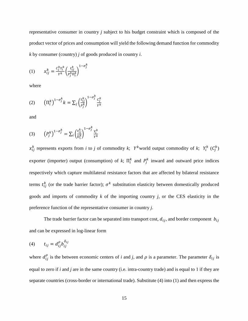
representative consumer in country j subject to his budget constraint which is composed of the

product vector of prices and consumption will yield the following demand function for commodity

k by consumer (country) j of goods produced in country i.

(1) 𝑥𝑖𝑗𝑘 =

𝐶𝑗𝑘𝑌𝑖

𝑘

𝑌𝑘 (𝑡𝑖𝑗

𝑘

𝑃𝑗𝑘Π𝑖

𝑘)1−𝜎𝑗

𝑘

where

(2) (Π𝑖𝑘)

1−𝜎𝑗𝑘

𝑘 = ∑ (𝑡𝑖𝑗

𝑘

𝑃𝑗𝑘)

1−𝜎𝑗𝑘

𝑗

𝐶𝑗𝑘

𝑌𝑘

and

(3) (𝑃𝑗𝑘)

1−𝜎𝑗𝑘

= ∑ (𝑡𝑖𝑗

𝑘

Π𝑖𝑘)

1−𝜎𝑗𝑘

𝑖𝑌𝑖

𝑘

𝑌𝑘

𝑥𝑖𝑗𝑘 represents exports from i to j of commodity k; 𝑌𝑘world output commodity of k; 𝑌𝑖

𝑘 (𝐶𝑗𝑘)

exporter (importer) output (consumption) of k; Π𝑖𝑘 and 𝑃𝑗

𝑘 inward and outward price indices

respectively which capture multilateral resistance factors that are affected by bilateral resistance

terms 𝑡𝑖𝑗𝑘 (or the trade barrier factor); 𝜎𝑘 substitution elasticity between domestically produced

goods and imports of commodity k of the importing country j, or the CES elasticity in the

preference function of the representative consumer in country j.

The trade barrier factor can be separated into transport cost, 𝑑𝑖𝑗, and border component 𝑏𝑖𝑗

and can be expressed in log-linear form

(4) 𝑡𝑖𝑗 = 𝑑𝑖𝑗𝜌

𝑏𝑖𝑗

𝛿𝑖𝑗

where 𝑑𝑖𝑗𝜌

is the between economic centers of i and j, and 𝜌 is a parameter. The parameter 𝛿𝑖𝑗 is

equal to zero if i and j are in the same country (i.e. intra-country trade) and is equal to 1 if they are

separate countries (cross-border or international trade). Substitute (4) into (1) and then express the

16

equation in log-linear form. This will result in the following estimable equation (omitting the

constant and the superscript k)

(5) 𝑥𝑖𝑗 = 𝑦𝑖 + 𝑐𝑗 + (1 − 𝜎𝑗)𝜌 ln 𝑑𝑖𝑗 + (1 − 𝜎𝑗)𝑑𝑖𝑗 ln 𝑏𝑖𝑗 − ln(Π𝑖)𝜎𝑗−1 − ln(𝑃𝑗)𝜎𝑗−1

where the lower case variables represent the natural logarithms of their uppercase variables.

Equation (5) is a gravity equation. But the main difficulty in estimating (5) is that it involves

unobservable multilateral resistance factors, Π𝑖 and 𝑃𝑗. These factors capture the cost of bilateral

trade between two countries relative to the average trade cost of country with the rest of its trading

partners. Anderson and Van Wincoop (2003) refer these multilateral resistance factors as the

substitutability between the country’s different trading partners. Traditional gravity equations omit

these relative trade costs. The omission leads to misspecification error.

There are three suggested ways of estimating (5): (a) the use of consumer price index to

measure the price effects in the gravity equation; (b) the use of non-linear least squares to solve

the system of equations involving (1) and (2); and (c) the use of country dummies to capture the

multilateral resistance factors. Feenstra (2002) argued that only (b) and (c) approaches lead to

consistent estimates. However, approach (b) entails complex computer programming. The use of

country dummies in approach (c) is preferable because equation (5) can be estimated using fixed

effects. Another advantage of using approach (c) is that the fixed effects estimation will eliminate

any other unobservable variables omitted in the trade cost functions in (4). In estimating (5)

approach (c) was used.

Equation (5) can further be simplified into the following estimating equation

(6) 𝑥𝑖𝑗 = 𝛽0 + 𝜃𝑖 + 𝜆𝑗 + (1 − 𝜎𝑗)𝜌 ln 𝑑𝑖𝑗 + 𝛾𝑗𝛿𝑖𝑗 + (1 − 𝜎𝑗)휀𝑖𝑗

where 𝛽0 is the constant term; 𝜃𝑖 = 𝑦𝑖 − (1 − 𝜎𝑗) ln Π𝑖 is a fixed effect of the exporting country;

𝜆𝑗 = 𝑐𝑗 − (1 − 𝜎𝑗) ln P𝑗 a fixed effect of the importing country; and 휀𝑖𝑗the error term. Aside from

17

the fixed effects, the key parameters to be estimated in (6) are the distance coefficient (1 − 𝜎𝑗)𝜌

and border coefficient 𝛾𝑗 = (1 − 𝜎𝑗). The border coefficient is [−𝑒𝑥𝑝(−𝛾𝑗)], where 𝑒𝑥𝑝 is anti-

log. The border coefficient shows how much trade within a country is above the international trade

due to cross border measures such as tariffs, NTBs, and all other factors that limit the flow of

goods internationally. As shown by Anderson and van Wincoop (2004), the formula of ad valorem

(AVE) tariff equivalent of border barriers facing exports from country i and country j is

(7) 𝑡𝑖𝑗 = 𝑒𝑥𝑝 (𝛾𝑗

𝜎𝑗) − 1

There were two databases used to estimate the gravity equation in (6). Data on country

exports, production, consumption, tariffs, and export taxes were from the GTAP 8. Information of

the other variables such as distance between major ports of trading countries, and other country-

specific geographical variables such as whether trading countries are contiguous or not, whether

they share common official language or not were taken from the GeoDist database (Mayer and

Zignago, 2011).

The GTAP 8 contains the 2007 data on 57 commodities of 129 countries and regions. The

data of 42 countries were used in the regression. These countries include the 8 countries in the

ASEAN, the additional 6 countries in the RCEP, 3 countries in the North American Free Trade

Agreement (NAFTA), and 25 countries in the European Union. Cororaton (2015) provides the list

of countries in the database used in the regression and the mapping of commodities to the GTAP

8 database. Table 4 summarizes the average AVE of NTBs in RCEP.

Table 4. Estimates of Average AVE of NTBS in RCEP

Agri-Food Crops Cereals Sugar Meat Dairy-Milk Manu. Services

RCEP 11.63 17.15 20.43 17.13 12.02 16.68 2.49 28.31

Source: Author’s calculations

18

Tariff Rates. The tariff rates applied by each country/region on imports from each of the

import origins were calibrated from the GTAP 8 database. Over the past couple of decades the

series of tariff reduction programs implemented globally under the World Trade Organization

(WTO) and regionally under the various regional trading agreements have lowered quite

considerably the level of tariff rates across countries. However, despite the trade reform programs,

tariff rates in a few commodities remain high, especially those goods that fall under the special

product categories. Table 5 presents the applied tariff rates computed from GTAP 8.

19

Table 5. Tariff Rates S1 S2 S3 S4 S5 S6 S7 S8 S9 S10 S11 S12 S13 S14 S15 S16

AUS 0.00 0.00 0.00 0.02 0.01 0.01 0.00 0.02 0.02 0.08 0.13 0.02 0.03 0.05 0.01 0.03

NZL 0.00 0.00 0.00 0.02 0.00 0.01 0.00 0.02 0.02 0.04 0.13 0.01 0.03 0.04 0.01 0.03

JPN 3.14 0.22 0.39 0.84 0.01 0.11 0.04 0.00 0.10 0.06 0.07 0.01 0.00 0.00 0.00 0.02

KOR 0.03 2.18 0.10 0.51 0.61 0.16 0.59 0.03 0.32 0.07 0.10 0.04 0.01 0.04 0.01 0.03

CHN 0.46 0.14 0.40 0.07 0.09 0.07 0.11 0.04 0.10 0.10 0.12 0.23 0.04 0.06 0.02 0.04

IND 0.52 0.82 0.83 0.33 0.60 0.15 0.27 0.12 0.47 0.15 0.14 0.14 0.17 0.13 0.04 0.13

MYS 0.31 0.00 0.00 0.02 0.01 0.01 0.20 0.05 0.16 0.07 0.11 0.03 0.08 0.04 0.00 0.05

PHL 0.40 0.07 0.21 0.02 0.06 0.09 0.06 0.04 0.07 0.07 0.10 0.04 0.03 0.04 0.01 0.05

SGP 0.00 0.00 0.00 0.00 0.00 0.00 0.00 0.00 0.01 0.00 0.00 0.00 0.00 0.00 0.00 0.00

VNM 0.16 0.06 0.20 0.13 0.11 0.11 0.10 0.07 0.26 0.20 0.26 0.06 0.03 0.09 0.06 0.09

IDN 0.08 0.02 0.16 0.04 0.02 0.02 0.02 0.03 0.09 0.06 0.10 0.03 0.03 0.04 0.01 0.04

THA 0.10 0.09 0.16 0.14 0.17 0.10 0.13 0.05 0.15 0.08 0.38 0.07 0.03 0.10 0.01 0.22

KHM 0.06 0.04 0.07 0.13 0.06 0.16 0.08 0.08 0.19 0.08 0.20 0.08 0.10 0.14 0.13 0.13

LAO 0.05 0.02 0.04 0.05 0.05 0.13 0.14 0.03 0.23 0.06 0.07 0.07 0.04 0.09 0.06 0.08

EAS 0.02 0.01 0.06 0.04 0.02 0.03 0.04 0.02 0.07 0.03 0.04 0.02 0.01 0.03 0.01 0.01

NAFTA 0.03 0.02 0.16 0.29 0.01 0.02 0.02 0.01 0.03 0.08 0.09 0.01 0.01 0.01 0.00 0.02

EU25 0.14 0.06 0.39 0.19 0.05 0.10 0.04 0.01 0.08 0.05 0.07 0.01 0.01 0.01 0.01 0.02

LTN 0.08 0.04 0.14 0.11 0.08 0.05 0.07 0.05 0.12 0.13 0.14 0.05 0.07 0.09 0.06 0.10

AFR 0.08 0.07 0.16 0.15 0.09 0.09 0.10 0.07 0.15 0.16 0.25 0.07 0.09 0.08 0.05 0.12

ROW 0.14 0.05 0.12 0.11 0.09 0.13 0.07 0.05 0.15 0.08 0.09 0.10 0.04 0.06 0.03 0.06

Source: GTAP 8

AUS Australia IDN Indonesia S1 Rice S9 All other food

NZL New Zealand THA Thailand S2 Wheat and all other cereals S10 Textile

JPN Japan KHM Cambodia S3 Sugar S11 Wearing apparel

KOR Korea LAO Lao Peoples Dem Rep. S4 Milk S12 Petroleum and chemical

CHN China EAS Rest of East Asia S5 Oils fats S13 Metal products

IND India NAFTA North America Free Trade S6 Meat S14 Transport and machinery

MYS Malaysia EU25 European Union 25 S7 All other agriculture S15 Electronic equipment

PHL Philippines LTN Latin America S8 Mining S16 All other manufacturing

SGP Singapore AFR Africa

VNM Viet Nam ROW Rest of the World

20

Foreign Investments. One of the benefits of participating in trade agreements is the

expected increase in the volume of trade flows among the participating parties as trade barriers are

minimized. Another benefit that normally goes with higher volume of trade is higher investment

flows and active transfer of technology among the participating parties. The Philippines is located

in a dynamic zone in Asia where a rapid increase in inflows of FDI has been observed in the past

couple of decades. Unfortunately, the inflows of FDI into the Philippines have been low; the

country has been underperforming in terms of attracting FDI. Using a concept called global FDI

frontier, Petri, Plummer, and Zhai (2012) have shown that the stock of FDI inflows as of 2006 into

the Philippine are significantly below the global FDI frontier by about US$30 – 40 billion (Table

6). The Philippines has a large absorptive capacity for higher inflows of FDI given its large and

young population base and educated work force and its rich natural resources. Thus, the country

may be able to improve its FDI performance as it seeks deeper integration with its trading partners

in the TPP, especially with the United States and Japan, the two major sources of FDI in the

Philippines.

Table 6. Alternative Foreign Direct Investment Scenarios (US$ millions)

Actual FDI Alternative estimated stocks (2006)

stock (2006) Top 3 years 75th percentile 1/2 to 90th

ASEAN 420,025 536,993 648,178 643,649

Brunei 9,861 19,057 15,312 15,312

Cambodia 2,954 3,245 3,481 3,969

Indonesia 19,056 77,545 178,794 134,655

Lao 856 1,209 1,686 1,599

Malaysia 53,575 90,704 73,067 78,074

Myanmar 5,005 7,165 6,378 7,280

Philippines 17,120 17,849 57,364 48,757

Singapore 210,089 211,070 210,521 210,521

Thailand 68,068 68,928 101,180 104,599

Vietnam 33,451 40,221 36,395 38,883

Source: Petri, Plummer, and Zhai (2011).

21

3. Definition of Simulation

To analyze the potential effects of the RCEP, a baseline and a reduction in trade barrier in

RCEP scenarios were simulated using the global CGE model. The details of the scenarios are:

Baseline. This is also called the business as usual (BaU) scenario. The global CGE was

simulated for 10 years (T1 to T10) using the projected GDP growth of the United States

Department of Agriculture/Economic Research Service (USDA/ERS) and the population

projection of the United Nations. A calibrated (pre-solved) multifactor productivity in each

country/region is used to ensure that the model replicates exactly the real GDP used in the baseline.

Reduction in Trade Barriers in RCEP. The trade barriers in RCEP were reduced starting in

T1 until T10. RCEP negotiations are still ongoing and no definite agreements have been reached

as of October 2015. For this reason, an assumed adjustment is hypothesized in the paper to occur

in the following manner. The applied tariffs in RCEP were reduced in the simulation from the

current level by 80 percent over the 10-year period (T1 to T10). Tariffs were reduced using a

geometric growth formula and no exceptions are provided for special products.

Issues related to NTBs are sometimes contentious, and their negotiations are quiet involved

and their resolutions are often times protracted. Thus, the reduction in NTBs is expected to be

much lower compared to the reduction in tariff rates over the 10-year period. In the analysis, the

AVE of NTBs in RCEP were by 10 percent. The NTBs were reduced using a geometric growth

formula over the 10-year period (T1 to T10). Both tariffs and NTBs in non-RCEP countries were

retained.

Furthermore, this simulation assumes a gradual increase in foreign investment inflows into

the Philippine over the 10 year period. The increase in the inflow was calculated using a geometric

growth formula. Over this period, the inflows were increased by US$2.5 billion, which is about 50

22

percent of the total foreign investment in 2009-2013. However, this level is significantly less

compared to the amount needed for the Philippines to move towards the FDI frontier in Table 6

estimated by Petri, Plummer, and Zhai (2012).

4. Simulation Results

This section presents the trade creation and trade diversion effects of RCEP at the regional

level as well as at the country members. Detailed effects on the Philippine economy is also

discussed. To facilitate the analysis, the results are presented as percentage differences from the

baseline over the simulation period from T1 to T10. The trade barriers outside of RCEP are

retained during the simulation.

Regional and Country Effects. Table 7 summarizes the gains from trade in RCEP and the

loss in regions outside RCEP. The total exports in RCEP increases from 0.6 percent relative to the

baseline in T1, and improves further over time to 3.3 percent in T10. There are notable trade

creation effects within RCEP as indicated by higher exports within the area. Exports within RCEP

improve from 1.9 percent relative to the baseline in T1 and to 9.9 percent in T10. There are

however diversion of exports as indicated by RCEP’s declining exports to the countries outside of

the area. RCEP’s exports to the rest of the world decline from -0.2 percent in T1 to -1.1 percent in

T10.

The results indicate that within RCEP, ASEAN as a whole has relatively smaller positive

exports effects compared to “+6”. ASEAN’s exports within RCEP increase by 1 percent in T1,

relatively smaller compared to the export improvement in “+6”, which is 2.3 percent. In T10, the

increase in ASEAN’s exports within the area is 5.4 percent, which is lower than the 12.3 percent

23

improvement in “+6”. The total exports of countries outside RCEP decline, largely due to the

declining exports to RCEP.

Table 7. Regional Effects, % change from Baseline

Initial T1 T2 T3 T4 T5 T6 T7 T8 T9 T10

RCEP

Total Exports 0.00 0.60 1.11 1.57 1.95 2.28 2.56 2.80 3.00 3.17 3.31

To RCEP 0.00 1.87 3.48 4.83 5.99 6.97 7.80 8.48 9.04 9.51 9.89

To Outside RCEP 0.00 -0.20 -0.37 -0.51 -0.63 -0.74 -0.84 -0.92 -1.00 -1.07 -1.14

ASEAN

Total Exports 0.00 0.44 0.83 1.16 1.42 1.64 1.81 1.94 2.05 2.14 2.21

To RCEP 0.00 1.03 1.95 2.70 3.34 3.87 4.32 4.69 4.99 5.24 5.44

To Outside RCEP 0.00 -0.20 -0.36 -0.52 -0.69 -0.86 -1.04 -1.21 -1.39 -1.56 -1.73

"+6"

Total Exports 0.00 0.65 1.20 1.70 2.12 2.49 2.80 3.08 3.32 3.51 3.68

To RCEP 0.00 2.26 4.20 5.86 7.30 8.51 9.55 10.42 11.15 11.76 12.27

To Outside RCEP 0.00 -0.20 -0.37 -0.51 -0.62 -0.71 -0.79 -0.85 -0.91 -0.95 -1.00

Non-RCEP

Total Exports 0.00 -0.02 -0.04 -0.06 -0.08 -0.09 -0.10 -0.11 -0.12 -0.13 -0.14

To RCEP 0.00 -0.26 -0.51 -0.71 -0.88 -1.03 -1.16 -1.27 -1.37 -1.46 -1.53

To Outside RCEP 0.00 0.02 0.05 0.06 0.08 0.10 0.12 0.14 0.15 0.17 0.18

Source: Author's calculations

The export effects vary significantly across the member countries as indicated in Table 8.

Within ASEAN, Indonesia benefits the most in terms of higher exports within RCEP. However,

Indonesia’s exports to the rest of the world decline. Vietnam benefits both in terms of higher

exports within RCEP and exports to the rest of the world. Although Cambodia benefits from higher

exports within RCEP, this is offset by the reduction in its exports to the rest of the world. The net

export effects in Malaysia and Thailand are smaller because of negative exports to the rest of the

world. Philippine exports within RCEP improve. Initially, its exports to the rest of the world

decline, but they recover towards T10.

24

The export effects across “+6” countries vary as well. Japan benefits the most in terms of

higher exports within RCEP. There are also notable improvements in exports of China, Australia,

and New Zealand within RCEP. India benefits from higher exports within RCEP and as well as

exports to the rest of the world.

Table 8. Country-Level Effects, % change from the baseline Initial T1 T2 T3 T4 T5 T6 T7 T8 T9 T10

ASEAN

Philippines

Total Exports 0.00 -0.16 0.16 0.53 0.87 1.20 1.53 1.84 2.13 2.40 2.65

To RCEP 0.00 0.11 0.63 1.16 1.63 2.07 2.49 2.87 3.21 3.50 3.76

To Outside RCEP 0.00 -0.58 -0.55 -0.44 -0.32 -0.19 -0.02 0.15 0.32 0.50 0.66

Malaysia

Total Exports 0.00 0.35 0.56 0.69 0.74 0.73 0.68 0.61 0.52 0.42 0.32

To RCEP 0.00 0.92 1.61 2.11 2.48 2.73 2.90 3.00 3.04 3.05 3.04

To Outside RCEP 0.00 -0.20 -0.45 -0.71 -0.99 -1.29 -1.59 -1.89 -2.17 -2.45 -2.71

Singapore

Total Exports 0.00 0.35 0.66 0.95 1.20 1.43 1.62 1.80 1.97 2.12 2.25

To RCEP 0.00 0.90 1.65 2.29 2.83 3.28 3.66 3.98 4.25 4.48 4.68

To Outside RCEP 0.00 -0.30 -0.53 -0.68 -0.80 -0.90 -0.96 -1.01 -1.05 -1.08 -1.10

Vietnam

Total Exports 0.00 1.06 1.95 2.66 3.26 3.74 4.10 4.38 4.59 4.75 4.86

To RCEP 0.00 1.65 3.01 4.06 4.94 5.63 6.16 6.59 6.92 7.18 7.38

To Outside RCEP 0.00 0.62 1.16 1.59 1.95 2.23 2.41 2.53 2.58 2.59 2.55

Indonesia

Total Exports 0.00 0.72 1.35 1.92 2.43 2.88 3.27 3.63 3.95 4.23 4.48

To RCEP 0.00 1.63 3.17 4.48 5.73 6.81 7.79 8.64 9.39 10.04 10.61

To Outside RCEP 0.00 -0.48 -0.97 -1.44 -1.92 -2.36 -2.77 -3.15 -3.50 -3.82 -4.11

Thailand

Total Exports 0.00 0.51 0.88 1.17 1.37 1.50 1.59 1.63 1.64 1.63 1.59

To RCEP 0.00 1.18 2.10 2.84 3.43 3.89 4.25 4.52 4.72 4.86 4.95

To Outside RCEP 0.00 -0.10 -0.23 -0.38 -0.57 -0.76 -0.97 -1.19 -1.42 -1.65 -1.88

Cambodia

Total Exports 0.00 0.62 0.94 1.06 1.01 0.83 0.55 0.24 -0.09 -0.42 -0.74

To RCEP 0.00 1.29 2.22 2.97 3.47 3.86 4.13 4.36 4.54 4.68 4.81

To Outside RCEP 0.00 0.52 0.75 0.78 0.64 0.38 0.02 -0.39 -0.81 -1.24 -1.64

Laos

Total Exports 0.00 0.39 0.74 1.06 1.33 1.57 1.78 1.97 2.13 2.27 2.38

To RCEP 0.00 0.51 0.94 1.32 1.64 1.90 2.13 2.33 2.48 2.61 2.70

To Outside RCEP 0.00 0.23 0.47 0.69 0.91 1.10 1.28 1.45 1.60 1.74 1.88

"+6"

Australia

Total Exports 0.00 0.73 1.40 2.01 2.56 3.05 3.49 3.88 4.24 4.56 4.85

To RCEP 0.00 1.55 3.00 4.25 5.42 6.43 7.34 8.13 8.84 9.47 10.02

To Outside RCEP 0.00 -0.48 -0.94 -1.38 -1.80 -2.17 -2.51 -2.84 -3.15 -3.45 -3.73

New Zealand

Total Exports 0.00 0.48 0.88 1.26 1.59 1.88 2.14 2.39 2.61 2.82 3.01

To RCEP 0.00 1.46 2.70 3.82 4.81 5.64 6.36 7.02 7.61 8.13 8.59

To Outside RCEP 0.00 -0.31 -0.58 -0.84 -1.06 -1.25 -1.42 -1.58 -1.74 -1.88 -2.01

Japan

Total Exports 0.00 0.88 1.66 2.37 3.02 3.58 4.09 4.58 5.03 5.44 5.82

To RCEP 0.00 3.25 6.12 8.63 10.88 12.79 14.49 15.98 17.27 18.40 19.38

25

To Outside RCEP 0.00 -0.75 -1.42 -1.99 -2.52 -2.96 -3.34 -3.71 -4.05 -4.35 -4.62

Korea

Total Exports 0.00 0.60 1.10 1.51 1.85 2.14 2.37 2.58 2.75 2.89 3.02

To RCEP 0.00 1.69 3.12 4.25 5.21 5.97 6.61 7.12 7.54 7.87 8.15

To Outside RCEP 0.00 -0.27 -0.50 -0.68 -0.85 -0.99 -1.11 -1.23 -1.34 -1.45 -1.55

China

Total Exports 0.00 0.54 0.99 1.40 1.74 2.05 2.29 2.50 2.68 2.82 2.93

To RCEP 0.00 2.00 3.72 5.17 6.43 7.48 8.36 9.10 9.72 10.24 10.68

To Outside RCEP 0.00 0.01 0.00 0.02 0.02 0.03 0.03 0.02 0.01 -0.01 -0.04

India

Total Exports 0.00 0.52 0.99 1.39 1.74 2.04 2.29 2.51 2.70 2.85 2.99

To RCEP 0.00 1.59 2.94 4.04 4.97 5.72 6.34 6.86 7.29 7.65 7.95

To Outside RCEP 0.00 0.27 0.53 0.76 0.96 1.14 1.30 1.42 1.53 1.61 1.68

Source: Author's calculations

Philippine Effects. Table 9 summarizes the effects of RCEP across Philippine sectors. Rice,

which is the most protected sector in the country, is negatively affected by the reduction in trade

barriers within RCEP. Rice output declines by 4.3 percent relative to the baseline in T10. Another

sector that is negatively affected is the textile sector. However, the inflow of cheaper textile

imports benefits the wearing apparel sector. The sector that benefits the most is construction,

mainly due to higher inflows of foreign investments. Output of the transportation and machinery

equipment sector improves along with the increase in the construction sector. Output of the

electronic equipment sector, which produces the country’s largest export item, declines initially,

but recovers over time. There are notable positive output effects in the service sectors, particularly

in the transportation sector which benefits from the improvement in agriculture and manufacturing.

Table 9. Philippine Sectoral Output, % change from baseline

Initial T1 T2 T3 T4 T5 T6 T7 T8 T9 T10

Rice 0.00 -0.91 -1.59 -2.11 -2.63 -3.07 -3.38 -3.67 -3.91 -4.10 -4.26

Wheat and all other cereals 0.00 -0.07 0.05 0.16 0.25 0.31 0.36 0.40 0.43 0.44 0.45

Sugar 0.00 -0.22 -0.11 0.03 0.17 0.31 0.49 0.65 0.81 0.98 1.13

Milk 0.00 -0.24 0.08 0.46 0.82 1.18 1.54 1.89 2.21 2.51 2.79

Oils fats 0.00 -0.42 -0.43 -0.36 -0.28 -0.18 -0.04 0.11 0.27 0.42 0.57

Meat 0.00 0.14 0.39 0.63 0.87 1.12 1.39 1.65 1.92 2.18 2.44

All other agriculture 0.00 0.03 0.32 0.57 0.75 0.91 1.06 1.18 1.27 1.35 1.41

Mining 0.00 -0.23 -0.18 0.05 0.42 0.88 1.45 2.12 2.82 3.55 4.30

All other food 0.00 0.07 0.51 0.93 1.32 1.68 2.02 2.34 2.65 2.92 3.18

26

Textile 0.00 -0.83 -1.15 -1.35 -1.52 -1.63 -1.65 -1.61 -1.53 -1.41 -1.28

Wearing apparel 0.00 -0.16 0.14 0.49 0.81 1.13 1.45 1.77 2.07 2.37 2.65

Petroleum and chemical prod. 0.00 -0.27 -0.05 0.23 0.50 0.80 1.13 1.49 1.85 2.20 2.55

Metal products 0.00 -0.32 -0.11 0.21 0.59 1.02 1.53 2.09 2.67 3.27 3.87

Transport and Machinery equip. 0.00 0.04 0.65 1.34 2.07 2.85 3.67 4.55 5.43 6.30 7.17

Electronic equipment 0.00 -0.42 -0.36 -0.20 -0.03 0.14 0.33 0.50 0.66 0.80 0.91

All other manufacturing 0.00 -0.33 -0.14 0.13 0.40 0.69 1.01 1.36 1.70 2.03 2.36

Utilities 0.00 -0.01 0.35 0.71 1.07 1.43 1.82 2.21 2.61 3.00 3.38

Construction 0.00 2.13 3.13 3.83 4.71 5.70 6.70 7.76 8.88 10.04 11.21

Trade 0.00 0.04 0.41 0.79 1.17 1.56 1.95 2.34 2.73 3.10 3.46

Transportation 0.00 0.14 0.62 1.08 1.52 1.96 2.40 2.85 3.29 3.72 4.14

Communications 0.00 -0.02 0.36 0.75 1.14 1.53 1.92 2.31 2.70 3.07 3.43

Finance business services 0.00 -0.11 0.22 0.59 0.95 1.32 1.70 2.09 2.48 2.85 3.22

Other services 0.00 0.02 0.52 0.99 1.47 1.92 2.37 2.81 3.24 3.65 4.04

Public administration 0.00 0.01 0.10 0.19 0.27 0.34 0.42 0.50 0.57 0.65 0.72

Source: Author's calculations

Table 10 presents the effects on factor prices. The results indicate higher improvement in

the returns to land largely due to the improvement in agricultural output. The improvement in

wages and in the returns to capital are higher relative to the returns to land initially in T1, but over

time the improvement in the returns to land surpasses the increase in all other factor prices. The

returns to capital decline over time. The increase in wages of skilled labor is slightly higher

compared to the improvement in wages of unskilled labor.

Table 10. Factor Price Effects, % change from baseline

Initial T1 T2 T3 T4 T5 T6 T7 T8 T9 T10

Skilled wages 0.00 0.88 1.24 1.56 1.91 2.26 2.60 2.94 3.26 3.58 3.88

Unskilled wages 0.00 0.95 1.25 1.54 1.87 2.21 2.54 2.87 3.19 3.50 3.80

Returns to capital 0.00 0.77 0.69 0.55 0.42 0.27 0.08 -0.12 -0.33 -0.53 -0.74

Returns to land 0.00 0.60 1.00 1.50 2.03 2.62 3.27 3.88 4.49 5.10 5.69

Source: Author's calculations

The Philippine macro effects presented in Table 11 are expressed in 2013 prices. The

results indicate that RCEP generates higher Philippine real GDP growth of 3 percent in 2023

27

relative to the baseline. From US$272 billion GDP in 2013, Philippine GDP increases to US$450

billion in 2023 in 2013 prices. RCEP also results in higher Philippine welfare as indicated by

positive equivalent variation (EV). Expressed in 2013 prices, the EV is US$2 billion in 2023.

Table 11. Philippine Macro Effects

2013 2014 2015 2016 2017 2018 2019 2020 2021 2022 2023

Real GDP, % change from baseline 0.00 0.00 0.29 0.61 0.92 1.25 1.59 1.94 2.28 2.62 2.95

Real GDP, US$ billion 272.1 285.8 301.0 317.2 334.2 351.2 369.2 388.1 407.9 428.7 450.1

Equivalent Variation, US$ billion 0.00 0.06 0.18 0.33 0.49 0.67 0.87 1.12 1.39 1.70 2.04

Source: Author's calculations

The positive factor price effects presented in Table 10 translate to higher real household

income effects (Table 12). The higher positive effects on the returns to land and labor wages lead

to higher increase in real income in the first decile relative to the 10th decile. Thus, despite the

reduction in output of the rice sector shown in Table 9, the effects of RCEP are generally

progressive in the sense that they favor lower income household groups.

Table 12. Real Household Income Effects in the Philippines, % change from baseline

Households Initial T1 T2 T3 T4 T5 T6 T7 T8 T9 T10

H1 0.00 0.26 0.73 1.26 1.79 2.34 2.93 3.48 4.05 4.60 5.13

H2 0.00 0.12 0.44 0.84 1.27 1.74 2.28 2.79 3.31 3.83 4.33

H3 0.00 0.13 0.46 0.87 1.31 1.79 2.33 2.84 3.37 3.89 4.40

H4 0.00 0.12 0.45 0.85 1.29 1.76 2.30 2.81 3.33 3.85 4.36

H5 0.00 0.13 0.44 0.85 1.27 1.74 2.26 2.76 3.28 3.79 4.29

H6 0.00 0.12 0.44 0.84 1.26 1.72 2.24 2.74 3.26 3.77 4.27

H7 0.00 0.16 0.48 0.88 1.30 1.76 2.28 2.78 3.29 3.81 4.31

H8 0.00 0.18 0.51 0.90 1.33 1.79 2.31 2.82 3.34 3.86 4.37

H9 0.00 0.16 0.47 0.86 1.27 1.73 2.23 2.73 3.24 3.76 4.27

H10 0.00 0.10 0.41 0.82 1.24 1.70 2.23 2.74 3.27 3.80 4.33

Source: Author's calculations

28

The progressive effects of RCEP on the Philippines can also be observed from the

reduction in the poverty index shown in Table 13. Over the 10 year simulation period, the poverty

incidence declines from 24.9 percent to 23.3 percent. Among poor households, those under

extreme poverty (P2) benefit the most as indicated by a higher decline in the index. The poverty

results also indicate that the reduction in urban poor is relatively higher compared to rural poor. In

addition, the GINI coefficient declines, indicating favorable distributional effects.

Table 13. Poverty Effects in the Philippines End of simulation period: T10

2012 /1/ Index % change from 2012

Philippines

P0 /2/ 24.85 23.29 -6.26

P1 6.84 6.26 -8.39

P2 2.68 2.42 -9.76

Urban

P0 11.57 10.77 -6.94

P1 2.79 2.51 -10.01

P2 0.99 0.88 -11.40

Rural

P0 35.58 33.42 -6.09

P1 10.10 9.29 -8.03

P2 4.04 3.66 -9.44

GINI Coefficient 0.4713 0.4709 -0.080 Source: 2012 FIES and author's calculations

/1/ FIES

/2/ P0 - poverty incidence; P1 - poverty gap; P2 - poverty severity

5. Policy Insights

Significant progress has been achieved over the past three decades in reducing tariffs on

international trade under the World Trade Organization (WTO) and subsequently in the context of

regional and bilateral preferential trade agreements. However, there are still several agricultural

products that are protected by high tariffs and NTBs. Rice, cereals, sugar, and milk are still

29

protected by high trade barriers. One of the major goals of RCEP is the elimination of trade barriers

(tariff and NTBs).

The objective of the paper is to assess the potential effects of the reduction in trade barriers

in RCEP using a global CGE model. The simulation results indicate that RCEP exports within the

area increase while exports to countries outside the region decline. Exports of non-RCEP countries

exports to RCEP decline.

ASEAN exports within RCEP improve, but the increase is less than the improvement of

exports the other 6 non-ASEAN RCEP members. Within ASEAN, the effects vary. Indonesia

benefits the most in terms of higher exports within RCEP, but its exports to the rest of the world

decline. Vietnam benefits both in terms of higher exports within RCEP and exports to the rest of

the world. Although Cambodia benefits from higher exports within RCEP, this is offset by the

reduction in its exports to the rest of the world. The net export effects in Malaysia and Thailand

are smaller because of negative exports to the rest of the world. Philippine exports within RCEP

improve. Initially, its exports to the rest of the world decline, but they recover over time.

The export effects across “+6” countries vary as well. Japan benefits the most in terms of

higher exports within RCEP. There are also notable improvements in exports of China, Australia,

and New Zealand within RCEP. India benefits from higher exports within RCEP and as well as

exports to the rest of the world.

The paper also looks in detail the impact on the Philippine economy. The production of

rice, which is the most protected sector in the economy, declines as imported rice with lower prices

enter the market. This would greatly benefit lower income households since rice is a major item in

their food basket. The inflow of cheaper textile imports leads to lower textile production, but this

benefits the wearing apparel sector. The construction sector benefits from higher inflows of foreign

30

investments. Output of the transportation and machinery equipment sector improves along with

the increase in the construction sector. There are notable positive output effects in the service

sectors, particularly in the transportation sector which benefits from the improvement in

agriculture and manufacturing.

The returns to land and as well as wages improve while the returns to capital decline. These

effects are progressive in the sense that they favor lower income household groups. The effects

decrease the poverty incidence in 10 years from 24.9 percent at present to 23.3 percent in 2023. In

addition, the effects lower the GINI coefficient, indicating favorable distributional effects.

Philippine real GDP is higher by 3 percent as a result of RCEP. RCEP also generates

additional Philippine welfare of US$2 billion in 2023.

31

References

Anderson, J. E. and E. van Wincoop. 2003. Trade Costs. Journal of Economic Literature, XLII

(3), 691-751.

Baier, S. and J. Bergstrand. 2006. “Bonus Vetus OLS: A Simple Approach for Addressing the

‘Border Puzzle” and other Gravity-Equations Issues.

http://www3.nd.edu/~jbergstr/Working_Papers/BVOLSMarch2006.pdf

Befus, T., M. Brockmeier, and B. Bektasoglu. 2013. Comparing Gravity Model Specifications to

Estimate NTBs Using the GTAP Framework. GTAP Resource #3910

https://www.gtap.agecon.purdue.edu/resources/download/6013.pdf

Chang, K. and Hayakawa, K. 2010. Border Barriers in Agricultural Trade and the Impact of their

Elimination: Evidence from East Asia. The Developing Economies 48 (2), 232-246

Cheong, I. 2013. Negotiations for the Trans-Pacific Partnership Agreement: Evaluation and

Implications for East Asian Regionalism. ADBI Working Paper Series No. 428. Asian

Development Bank Institute: Tokyo, Japan.

Cockburn, J. (2001). Trade Liberalization and Poverty in Nepal: A Computable General

Equilibrium Micro Simulation Analysis, mimeo, Department of Economics, Laval

University.

Cororaton, C. B. (2013). Economic Impact Analysis of the Reduction in Sugar Tariffs Under the

ASEAN Trade in Goods Agreement: The Case of the Philippine Sugar Sector. Global

Issues Initiative Working Paper No. 2013-1. Virginia Polytechnic Institute and State

University, Arlington, Virginia (http://www.gii.ncr.vt.edu/docs/GII_WP2013-1.pdf)

Cororaton, C. B., and E. Corong (2009). Philippine Agricultural and Food Policies: Implications

on Poverty and Income Distribution. International Food Policy Research Institute (IFPRI)

Research Report No. 161. Washington DC: IFPRI.

Decaluwé, B., A. Patry, L. Savard and E. Thorbecke (2000). "Poverty Analysis within a General

Equilibrium Framework", Working paper 9909, Department of Economics, Laval

University.

Egger, P., J. Francois, M. Manchin, and D. Nelson. 2014. Non-Tariff Barriers, Integration, and the

Trans-Atlantic Economy http://econ.tulane.edu/seminars/Nelson_Barriers.pdf

Feenstra, R. 2002. Border Effects and Gravity Equation: Consistent Methods for Estimation.

Scottish Journal of Political Economy. 49(5), 491-506.

Fergusson, I., and B. Vaughn. 2010. The Trans-Pacific Partnership. Congressional Research

Service 7-5700. Washington D.C.

32

Fugazza, M., and J. Maur. 2008. Non-Tariff Barriers in Computable General Equilibrium

Modeling. Policy Issues in International Trade and Commodities Study Series N. 38.

United Nations Conference on Trade and Development.

Ganuza, E., R. Barros, R., and R. Vos (2002). Labor Market Adjustment, Poverty and Inequality

During Liberalization. In Economic Liberalization, Distribution and Poverty: Latin

America in the 1990s. (Rob Vos, Lance Taylor and Ricardo Paes de Barros, R., eds)

Cheltenham (UK) and Northampton (US): Edward Elgar Publishing, pp. 54-88.

Ianchovichina, E. and T. Walmsley. 2012. GDyn Book: Dynamic Modeling and Applications in

Global Economic Analysis. Cambridge University Press: Cambridge, U.K.

Itakura, K, and H. Lee. 2012. Welfare Changes and Sectoral Adjustments of Asia-Pacific

Countries under Alternative Sequencings of Free Trade Agreements. Osaka School of

International Public Policy Discussion Paper DP-2012-E-005.

Mayer, T. and S. Zignago. 2011. “Notes of CEPII’s distance measures: The GeoDist database”.

CEPII Working Paper No. 2011-25. http://www.cepii.fr/PDF_PUB/wp/2011/wp2011-

25.pdf.

Olper. A. and V. Raimondi. 2008. Agricultural Market Integration in the OECD: A gravity-border

effect approach. Food Policy 33, 165-175

Petri, P., M. Plummer, and F. Zhai. 2012. The Trans-Pacific Partnership and Asia-Pacific

Integration: A Quantitative Assessment. 98 Policy Analyses in International Economics.

November. Peterson Institute for International Economics: Washington, D.C.

Petri, P., M. Plummer, and F. Zhai. 2012. “The ASEAN Economic Community: A General

Equilibrium Analysis”. Asian Economic Journal. Vol. 26. Issue 2. Pages 93-118.

Robichaud, V., A. Lemelin, H. Maisonnave and B. Decaluwe. 2011. The PEP Standard Multi-

Region, Recursive Dynamic World Model, PEP Global Model (PEP-w-t_v1_4.gms).

Available from URL: www.pep-net.org.

Winchester, N. 2009. Is there a dirty secret? Non-barriers and the gains from trade. Journal of

Policy Modeling. 32, 819-834.

Zhai, F. 2008. Armington Meets Meltiz: Introducing Firm Heterogeneity in a Global CGE Model

of Trade. Journal of Economic Integration 23(3), September, pp. 575-604.

33

Appendix A: Mapping to GTAP 8 Database

The GTAP 8 database contains information for 57 sectors in 129 countries/regions. To

facilitate the computation of the model solution and analysis of results, the database was

aggregated to 24 sectors in 20 countries/regions and used to calibrate the global CGE model. Table

14 presents the mapping of the 24 sectors in the model to 57 sectors the GTAP 8, while Table 15

the mapping of the 20 countries/regions to the 129 countries/regions in the database. The model

specifies each individual countries in the RCEP except for Brunei and Myanmar which are not in

the GTAP 8 database.

Table 14. Mapping of Global CGE Sectors to GTAP 8 Database Sectors

Global CGE model GTAP 8 Database Sectors

Sector

no. Description

Sector

no. Code Description

1 Rice 1 pdr Paddy rice

24 pcr Processed rice

2 Wheat 2 wht Wheat

3 Sugar 25 sgr Sugar

6 c_b Sugar cane-sugar beet

4 Milk/Dairy 11 rmk Raw milk

23 mil Dairy products

5 Oils/Fats 5 osd Oil seeds

22 vol Vegetable oils-fats

6 Meat 9 ctl Cattle-sheep-goats-horses

10 oap Animal products nec

20 cmt Meat-cattle-sheep-goats-horse

21 omt Meat products nec

7 Other Agriculture 3 gro Cereal grains nec

4 v_f Vegetables-fruit-nuts

7 pfb Plant-based fibers

8 ocr Crops nec

12 wol Wool-silk-worm cocoons

13 frs Forestry

14 fsh Fishing

8 Other Food 26 ofd Food products nec

27 b_t Beverages-tobacco products

9 Mining/Minerals 18 omn Minerals nec

19 nmm Mineral products nec

34

10 Textile 28 tex Textiles

11 Wearing apparel 29 wap Wearing apparel

12 Oil/Petroleum/Coal/Chem. 30 p_c Petroleum-coal products

15 coa Coal

16 oil Oil

17 gas Gas

31 crp Chemical-rubber-plastic prods

13 Metals 32 i_s Ferrous metals

33 nfm Metals nec

34 fmp Metal products

14

Transport/Machinery

Equip. 35 mvh Motor vehicles-parts

36 otn Transport equipment nec

37 ome Machinery-equipment nec

15 Electronics 38 ele Electronic equipment

16 Other Manufacturing 39 lea Leather products

40 lum Wood products

41 ppp Paper products-publishing

42 omf Manufactures nec

17 Utilities 43 ely Electricity

44 gdt Gas manufacture-distribution

45 wtr Water

18 Construction 46 cns Construction

19 Trade 47 trd Trade

20 Transport Services 48 otp Transport nec

49 wtp Sea transport

50 atp Air transport

21 Communications 51 cmn Communication

22 Finance/Business Services 52 ofi Financial services nec

53 isr Insurance

54 obs Business services nec

23 Other services 55 ros Recreation-other services

56 dwe Dwellings

24 Public Administration 57 osg PubAdmin-Defense-Health-Educ.

35

Table 15. Mapping of Global CGE Countries/Regions to GTAP 8 Countries/Regions

Global CGE GTAP 8 Database Countries/Regions

No. Code Description Code Description

1 1MYS Malaysia MYS Malaysia

2 1PHL Philippines PHL Philippines

3 1SGP Singapore SGP Singapore

4 1VNM Viet Nam VNM Viet Nam

5 1IDN Indonesia IDN Indonesia

6 1THA Thailand THA Thailand

7 1KHM Cambodia KHM Cambodia

8 1LAO Lao Peoples Dem. Rep LAO Lao Peoples Dem. Rep

9 1AUS Australia AUS Australia

10 1NZL New Zealand NZL New Zealand

11 1JPN Japan JPN Japan

12 1KOR Korea KOR Korea

13 1CHN China CHN China

14 1IND India IND India

15 1NFTA NAFTA CAN Canada

USA United States of America

MEX Mexico

16 1EU25 European Union 25 AUT Austria

BEL Belgium

CYP Cyprus

CZE Czech Republic

DNK Denmark

EST Estonia

FIN Finland

FRA France

DEU Germany

GRC Greece

HUN Hungary

IRL Ireland

ITA Italy

LVA Latvia

LTU Lithuania

LUX Luxembourg

MLT Malta

NLD Netherlands

POL Poland

PRT Portugal

SVK Slovakia

SVN Slovenia

36

ESP Spain

SWE Sweden

GBR United Kingdom

17 1LTN Latin America ARG Argentina

BOL Bolivia

BRA Brazil

CHL Chile

COL Colombia

ECU Ecuador

PRY Paraguay

URY Uruguay

VEN Venezuela

XSM Rest of South America

CRI Costa Rica

GTM Guatemala

HND Honduras

NIC Nicaragua

PAN Panama

1PER Peru

SLV El Salvador

XCA Rest of Central America

XCB Caribbean

18 1AFR Africa EGY Egypt

MAR Morocco

TUN Tunisia

XNF Rest of North Africa

CMR Cameroon

CIV Cote d_Ivoire

GHA Ghana

NGA Nigeria

SEN Senegal

XWF Rest of Western Africa

XCF Central Africa

XAC South Central Africa

ETH Ethiopia

KEN Kenya

MDG Madagascar

MWI Malawi

MUS Mauritius

MOZ Mozambique

TZA Tanzania

UGA Uganda

ZMB Zambia

37

ZWE Zimbabwe

XEC Rest of Eastern Africa

BWA Botswana

NAM Namibia

ZAF South Africa

XSC Rest of South African Custom

19 1EAS East Asia HKG Hong Kong

MNG Mongolia

TWN Taiwan

XEA Rest of East Asia

20 1ROW Rest of the World XOC Rest of Oceania

XSE Rest of Southeast Asia

BGD Bangladesh

NPL Nepal

PAK Pakistan

LKA Sri Lanka

XSA Rest of South Asia

XNA Rest of North America

CHE Switzerland

NOR Norway

XEF Rest of EFTA

ALB Albania

BGR Bulgaria

BLR Belarus

HRV Croatia

ROU Romania

RUS Russian Federation

UKR Ukraine

XEE Rest of Eastern Europe

XER Rest of Europe

KAZ Kazakhstan

KGZ Kyrgyzstan

XSU Rest of Former Soviet Union

ARM Armenia

AZE Azerbaijan

GEO Georgia

BHR Bahrain

IRN Iran Islamic Republic of

ISR Israel

KWT Kuwait

OMN Oman

QAT Qatar

SAU Saudi Arabia

38

TUR Turkey

ARE United Arab Emirates

XWS Rest of Western Asia

XTW Rest of the World

39

Appendix B: Specification of a Global CGE Model

Indices

The following are the indices used in the variables of the model

(i, j, ij): sectors

(m): imported commodities

(nm): non-imported, domestically produced commodities

(x): exports

(nx): domestically produced sold to the domestic market only

(z, zj): countries or regions

(k): capital type

(l): labor type

(t): period

Production

Sectoral value added (𝑉𝐴𝑗,𝑧,𝑡) is a fixed proportion of sectoral output (𝑋𝑆𝑗,𝑧,𝑡)

(B1) 𝑉𝐴𝑗,𝑧,𝑡 = 𝜐𝑗,𝑧𝑋𝑆𝑗,𝑧,𝑡

where (𝜐𝑗,𝑧) is a set of fixed value added coefficients.

Sectoral intermediate consumption is also a fixed proportion of sectoral output

(B2) 𝐶𝐼𝑗,𝑧,𝑡 = 𝑖𝑜𝑗,𝑧𝑋𝑆𝑗,𝑧,𝑡

where (𝑖𝑜𝑗,𝑧) is a set of fixed intermediate consumption coefficients.

Sectoral value added is a CES function of composite labor and composite capital. The

breakdown of these composite factor inputs is discussed below. Cost minimization by firms yields

40

the following first order conditions: the demand functions for the composite labor (𝐿𝐷𝐶𝑗,𝑧,𝑡) and

the composite capital (𝐾𝐷𝐶𝑗,𝑧,𝑡), and a unit cost function of value added (𝑃𝑉𝐴𝑗,𝑧,𝑡).

The demand for the composite labor is

(B3) 𝐿𝐷𝐶𝑗,𝑧,𝑡 = 𝛽𝐿𝐷𝐶,𝑗,𝑧

𝜎𝑉𝐴,𝑗,𝑧 (𝛿𝐿𝐷𝐶,𝑗,𝑧𝛼𝑉𝐴,𝑗,𝑧)𝜎𝑉𝐴,𝑗,𝑧−1

(𝑃𝑉𝐴𝑗,𝑧,𝑡

𝑊𝐶𝑗,𝑧,𝑡)

𝜎𝑉𝐴,𝑗,𝑧

𝑉𝐴𝑗,𝑧,𝑡

where (𝛽𝐿𝐷𝐶,𝑗.𝑍) is the composite labor share parameter, (𝛼𝑉𝐴,𝑗,𝑧) the scale parameter in the CES

function, (𝛿𝐿𝐷𝐶,𝑗,𝑧) the composite labor productivity factor, (𝜎𝑉𝐴,𝑗,𝑧) the elasticity of substitution

between the composite labor and the composite capital, (𝑊𝐶𝑗,𝑧,𝑡) the composite wage, and (𝑉𝐴𝑗,𝑧,𝑡)

the value added.

The demand for the composite capital is

(B4) 𝐾𝐷𝐶𝑗,𝑧,𝑡 = 𝛽𝐾𝐷𝐶,𝑗,𝑧

𝜎𝑉𝐴,𝑗,𝑧 (𝛿𝐾𝐷𝐶,𝑗,𝑧𝛼𝑉𝐴,𝑗,𝑧)𝜎𝑉𝐴,𝑗,𝑧−1

(𝑃𝑉𝐴𝑗,𝑧,𝑡

𝑅𝐶𝑗,𝑧,𝑡)

𝜎𝑉𝐴,𝑗,𝑧

𝑉𝐴𝑗,𝑧,𝑡

where (𝛽𝐾𝐷𝐶,𝑗.𝑍 ) is the composite capital share parameter, (𝛿𝐾𝐷𝐶,𝑗,𝑧) the composite capital

productivity factor, and (𝑅𝐶𝑗,𝑧,𝑡) the composite rental rate of capital.

The unit cost function of value added is

(B5) 𝑃𝑉𝐴𝑗,𝑧,𝑡 = (1

𝛼𝑉𝐴,𝑗,𝑧) (𝛽𝐿𝐷𝐶,𝑗,𝑧 (

𝑊𝐶𝑗,𝑧,𝑡

𝛿𝐿𝐷𝐶,𝑗,𝑧)

1−𝜎𝑉𝐴,𝑗,𝑧

+ 𝛽𝐾𝐷𝐶,𝑗,𝑧 (𝑅𝐶𝑗,𝑧,𝑡

𝛿𝐾𝐷𝐶,𝑗,𝑧)

1−𝜎𝑉𝐴,𝑗,𝑧

)

1

1−𝜎𝑉𝐴,𝑗,𝑧

where (𝑃𝑉𝐴𝑗,𝑧,𝑡) is the CES dual price; it is the aggregate price of the CES components: the prices

of composite labor and composite capital.

The composite labor is a CES function of two types of labor: (l ) = skilled and unskilled

labor. Cost minimization by firms will yield the following first order conditions: the demand

functions for each type of labor, and a unit cost function of the composite labor.

The demand for type l labor is

41

(B6) 𝐿𝐷𝑙,𝑗,𝑧,𝑡 = 𝛽𝑙,𝑗,𝑧

𝜎𝐿𝐷,𝑗,𝑧(𝛿𝑙,𝑗,𝑧𝛼𝐿𝐷,𝑗,𝑧)𝜎𝐿𝐷,𝑗,𝑧−1

(𝑊𝐶𝑗,𝑧,𝑡

𝑊𝑇𝐼𝑙,𝑗,𝑧,𝑡)

𝜎𝐿𝐷,𝑗,𝑧

𝐿𝐷𝐶𝑗,𝑧,𝑡

where (𝛽𝑙,𝑗.𝑍) is the share parameter of type l labor, (𝛿𝑙,𝑗,𝑧t) the productivity factor of type l labor,

(𝛼𝐿𝐷,𝑗,𝑧) the scale parameter in the CES function, (𝜎𝐿𝐷,𝑗,𝑧) the elasticity of substitution between the

two types of labor, and (𝑊𝑇𝐼𝑙,𝑗,𝑧,𝑡) the wage rate of type l labor including payroll tax.

The unit cost function of the composite labor is

(B7) 𝑊𝐶𝑗,𝑧,𝑡 = (1

𝛼𝐿𝐷,𝑗,𝑧) ( ∑ 𝛽𝑙,𝑗,𝑧𝑙 (

𝑊𝑇𝐼𝑙,𝑗,𝑧,𝑡

𝛿𝑙,𝑗,𝑧)

1−𝜎𝐿𝐷,𝑗,𝑧

)

1

1−𝜎𝐿𝐷,𝑗,𝑧

This is a CES dual price.

The composite capital is a CES function of two types of capital: (k) = physical capital and

land (which includes natural resources). However, land is only used in agriculture and mining

while physical capital in all sectors.

The demand for type k capital is

(B8) 𝐾𝐷𝑘,𝑗,𝑧,𝑡 = 𝛽𝑘,𝑗,𝑧

𝜎𝐾𝐷,𝑗,𝑧(𝛿𝑘,𝑗,𝑧𝛼𝐾𝐷,𝑗,𝑧)𝜎𝐾𝐷,𝑗,𝑧−1

(𝑅𝐶𝑗,𝑧,𝑡

𝑅𝑇𝐼𝑘,𝑗,𝑧,𝑡)

𝜎𝐾𝐷,𝑧

𝐾𝐷𝐶𝑗,𝑧,𝑡

where (𝛽𝑘,𝑗.𝑍) is the share parameter of type k capital, (𝛿𝑘,𝑗,𝑧t) the productivity factor of type k

capital, (𝛼𝐾𝐷,𝑗,𝑧) the scale parameter in the CES function, (𝜎𝐾𝐷,𝑗,𝑧) the elasticity of substitution

between the two types of capital, and (𝑅𝑇𝐼𝑘,𝑗,𝑧,𝑡) the rental rate of type k capital including factor

tax on capital.

The unit cost function of the composite capital is

(B9) 𝑅𝐶𝑗,𝑧,𝑡 = (1

𝛼𝐾𝐷,𝑗,𝑧) ( ∑ 𝛽𝑘,𝑗,𝑧𝑘 (

𝑅𝑇𝐼𝑘,𝑗,𝑧,𝑡

𝛿𝑘,𝑗,𝑧)

1−𝜎𝐾𝐷,𝑗,𝑧

)

1

1−𝜎𝐾𝐷,𝑗,𝑧

This is a CES dual price.

Income and Savings

42

In each region there is a single household and a government. Household income (𝑌𝐻𝑧,𝑡) is

composed of labor (𝑌𝐻𝐿𝑧,𝑡) and capital income (𝑌𝐻𝐾𝑧,𝑡).

(B10) 𝑌𝐻𝑧,𝑡 = 𝑌𝐻𝐿𝑧,𝑡 + 𝑌𝐻𝐾𝑧,𝑡

Labor income is the sum of labor earnings from the two types of labor, while capital income

is the sum of rentals paid for the two types of capital less depreciation. That is,

(B11) 𝑌𝐻𝐿𝑧,𝑡 = ∑ 𝑊𝑙,𝑧,𝑡𝐿𝐷𝑙,𝑗,𝑧,𝑡𝑙,𝑗

(B12) 𝑌𝐻𝐾𝑧,𝑡 = ∑ 𝑅𝑘,𝑗,𝑧,𝑡𝐾𝐷𝑘,𝑗,𝑧,𝑡𝑘,𝑗 − 𝐷𝑒𝑝𝑧,𝑡

where (𝑊𝑙,𝑧,𝑡) is the wage rate of type l labor before payroll tax, (𝑅𝑘,𝑗,𝑧,𝑡) the sectoral rental rate of

type k capital before rental tax, and (𝐷𝑒𝑝𝑧,𝑡) the amount of depreciation (capital consumption

allowance).

The household disposable income (𝑌𝐷𝐻𝑧,𝑡), the household consumption budget (𝐶𝑇𝐻𝑧,𝑡),

and the household savings (𝑆𝐻𝑧,𝑡 ) are

(B13) 𝑌𝐷𝐻𝑧,𝑡 = 𝑌𝐻𝑧,𝑡 − 𝑇𝐷𝐻𝑧,𝑡

(B14) 𝐶𝑇𝐻𝑧,𝑡 = 𝑌𝐷𝐻𝑧,𝑡 − 𝑆𝐻𝑧,𝑡

(B15) 𝑆𝐻𝑧,𝑡 = 𝑃𝐼𝑋𝐶𝑂𝑁𝑧,𝑡𝜂

𝑠ℎ0𝑧,𝑡 + 𝑠ℎ1𝑧𝑌𝐷𝐻𝑧,𝑡

where (𝑇𝐷𝐻𝑧,𝑡) is the household income tax, (𝑃𝐼𝑋𝐶𝑂𝑁𝑧,𝑡) the consumer price index, (𝑠ℎ0𝑧,𝑡) the

intercept in the savings function in t, (𝑠ℎ1𝑧) the slope of the savings function, and (𝜂) the price-

elasticity of indexed transfers and parameters.

Government

The revenue of the government (𝑌𝐺𝑧,𝑡) comes from three sources: household income tax

(𝑇𝐷𝐻𝑧,𝑡), production-related taxes (𝑇𝑃𝑅𝑂𝐷𝑁𝑧,𝑡), and products and imports taxes (𝑇𝑃𝑅𝐶𝑇𝑧,𝑡).

(B16) 𝑌𝐺𝑧,𝑡 = 𝑇𝐷𝐻𝑧,𝑡 + 𝑇𝑃𝑅𝑂𝐷𝑁𝑧,𝑡 + 𝑇𝑃𝑅𝐶𝑇𝑧,𝑡

43

Income taxes paid by households are a linear function of total income, i.e.,

(B17) 𝑇𝐷𝐻𝑧,𝑡 = 𝑃𝐼𝑋𝐶𝑂𝑁𝑧,𝑡𝜂

𝑡𝑡𝑑ℎ0𝑧,𝑡 + 𝑡𝑡𝑑ℎ0𝑧,𝑡𝑌𝐻𝑧,𝑡

The production-related taxes are: the taxes on payroll (𝑇𝐼𝑊𝑇𝑧,𝑡), the taxes on the use capital

(𝑇𝐼𝐾𝑇𝑧,𝑡), and the taxes on production (𝑇𝐼𝑃𝑇𝑧,𝑡).

(B18) 𝑇𝑃𝑅𝑂𝐷𝑁𝑧,𝑡 = 𝑇𝐼𝑊𝑇𝑧,𝑡 + 𝑇𝐼𝐾𝑇𝑧,𝑡 + 𝑇𝐼𝑃𝑇𝑧,𝑡

The tax on payroll is

(B19) 𝑇𝐼𝑊𝑇𝑧,𝑡 = ∑ 𝑇𝐼𝑊𝑙,𝑗,𝑧,𝑡𝑙,𝑗 = ∑ 𝑡𝑡𝑖𝑤𝑙,𝑗,𝑧,𝑡𝑊𝑙,𝑧,𝑡𝐿𝐷𝑙,𝑗,𝑧,𝑡𝑙,𝑗

where (𝑇𝐼𝑊𝑙,𝑗,𝑧,𝑡) is the revenue from payroll tax on type l labor, and (𝑡𝑡𝑖𝑤𝑙,𝑗,𝑧,𝑡) the rate of payroll

tax.

Similarly, the tax on the use of capital is

(B20) 𝑇𝐼𝐾𝑇𝑧,𝑡 = ∑ 𝑇𝐼𝐾𝑘,𝑗,𝑧,𝑡𝑘,𝑗 = ∑ 𝑡𝑡𝑖𝑘𝑘,𝑗,𝑧,𝑡𝑅𝑘,𝑗,𝑧,𝑡𝐾𝐷𝑘,𝑗,𝑧,𝑡𝑘,𝑗

where (𝑇𝐼𝐾𝑘,𝑗,𝑧,𝑡) is the revenue from the tax on the use of type k capital, and (𝑡𝑡𝑖𝑘𝑘,𝑗,𝑧,𝑡) the tax

rate on the use of capital.

The production tax is

(B21) 𝑇𝐼𝑃𝑇𝑧,𝑡 = ∑ 𝑇𝐼𝑃𝑗,𝑧,𝑡𝑗 = ∑ 𝑡𝑡𝑖𝑝𝑗,𝑧,𝑡𝑃𝑃𝑗,𝑧,𝑡𝑋𝑆𝑗,𝑧,𝑡𝑗

where (𝑇𝐼𝑃𝑗,𝑧,𝑡) is the revenue from the tax on production, (𝑡𝑡𝑖𝑃𝑗,𝑧,𝑡) the tax rate on the use of

capital, and (𝑃𝑃𝑗,𝑧,𝑡) the unit cost of sector j.

The taxes on products and imports are: the indirect taxes on commodities (𝑇𝐼𝐶𝑇𝑧,𝑡), the

duties levied on imports (𝑇𝐼𝑀𝑇𝑧,𝑡), and the export taxes (𝑇𝐼𝑋𝑇𝑧,𝑡).

(B22) 𝑇𝑃𝑅𝐶𝑇𝑆𝑧,𝑡 = 𝑇𝐼𝐶𝑇𝑧,𝑡 + 𝑇𝐼𝑀𝑇𝑧,𝑡 + 𝑇𝐼𝑋𝑇𝑧,𝑡

The indirect tax on commodities is

(B23) 𝑇𝐼𝐶𝑇𝑧,𝑡 = ∑ 𝑇𝐼𝐶𝑖,𝑧,𝑡𝑖

44

where (𝑇𝐼𝐶𝑖,𝑧,𝑡) is the revenue from indirect tax. Since commodities available in the domestic

market are composed of domestically produced goods and imports, (𝑇𝐼𝐶𝑖,𝑧,𝑡) has two components:

(𝑇𝐼𝐶𝑛𝑚,𝑧,𝑡) the indirect tax on non-imported commodities, and (𝑇𝐼𝐶𝑚,𝑧,𝑡) the indirect tax on

imported commodities.

The indirect tax on non-imported commodities is

(B24) 𝑇𝐼𝐶𝑛𝑚,𝑧,𝑡 = 𝑡𝑡𝑖𝑐𝑛𝑚,𝑧,𝑡𝑃𝐿𝑛𝑚,𝑧,𝑡𝐷𝐷𝑛𝑚,𝑧,𝑡

where (𝑡𝑡𝑖𝑐𝑛𝑚,𝑧,𝑡) is the indirect tax rate on non-imported commodities, (𝑃𝐿𝑛𝑚,𝑧,𝑡) the price of

locally produced commodities excluding taxes, and (𝐷𝐷𝑛𝑚,𝑧,𝑡) the domestic demand for

commodity nm.

Import duties are levied on commodities that enter the border. When these commodities

are moved beyond the border into the various domestic markets, similar to the domestically

produced goods, they are charged with indirect taxes as well. Moreover, the border price of imports

includes trade margins. Taking all these factors together, the indirect tax on imported commodities

(𝑇𝐼𝐶𝑚,𝑧,𝑡) is

(B25) 𝑇𝐼𝐶𝑚,𝑧,𝑡 = 𝑡𝑡𝑖𝑐𝑚,𝑧,𝑡{𝑃𝐿𝑚,𝑧,𝑡𝐷𝐷𝑚,𝑧,𝑡 ∑ [(1 + 𝑡𝑡𝑖𝑚𝑚,𝑧𝑗,𝑧,𝑡)(𝑃𝑊𝑀𝑚,𝑧𝑗,𝑧,𝑡 +𝑧𝑗

∑ 𝑃𝑊𝑀𝐺𝑖𝑗,𝑡𝑡𝑚𝑟𝑔𝑖𝑗,𝑚,𝑧𝑗,𝑧,𝑡𝑖𝑗 )𝑒𝑧,𝑡𝐼𝑀𝑚,𝑧𝑗,𝑧,𝑡]}

where (𝑡𝑡𝑖𝑐𝑚,𝑧,𝑡) the indirect tax rate on imports, (𝑡𝑡𝑖𝑚𝑚,𝑧𝑗,𝑧,𝑡) the rate of import duties,

(𝑃𝑊𝑀𝑚,𝑧𝑗,𝑧,𝑡) the world price of m imported from country/region zj by country/region z in

international currency, (𝑃𝑊𝑀𝐺𝑖𝑗,𝑡) the world price of trade margins in international currency,

(𝑡𝑚𝑟𝑔𝑖𝑗,𝑚,𝑧𝑗,𝑧,𝑡) the rate of international transport margin services, (𝑒𝑧,𝑡) the exchange rate, and

(𝐼𝑀𝑚,𝑧𝑗,𝑧,𝑡) imports.

The total government revenue (𝑇𝐼𝑀𝑇𝑧,𝑡) from duties on imports is given as

45

(B26) 𝑇𝐼𝑀𝑇𝑧,𝑡 = ∑ 𝑇𝐼𝑀𝑚,𝑧𝑗,𝑧,𝑡𝑚,𝑧𝑗 = ∑ 𝑡𝑡𝑖𝑚𝑚,𝑧𝑗,𝑧,𝑡(𝑃𝑊𝑀𝑚,𝑧𝑗,𝑧,𝑡 +𝑚,𝑧𝑗

𝑃𝑊𝑀𝑚,𝑧𝑗,𝑧,𝑡)𝑒𝑧,𝑡𝐼𝑀𝑚,𝑧𝑗,𝑧,𝑡

The total government revenue (𝑇𝐼𝑋𝑇𝑧,𝑡) from export taxes is defined as

(B27) 𝑇𝐼𝑋𝑇𝑧,𝑡 = ∑ 𝑇𝐼𝑋𝑥,𝑧,𝑧𝑗,𝑡𝑥,𝑧𝑗 = ∑ 𝑡𝑡𝑖𝑥𝑥,𝑧,𝑧𝑗,𝑡𝑃𝐸𝑥,𝑧,𝑧𝑗,𝑡𝐸𝑋𝑥,𝑧,𝑧𝑗,𝑡𝑥,𝑧𝑗

where (𝑇𝐼𝑋𝑥,𝑧,𝑧𝑗,𝑡) is the revenue from taxes on export by country/region z to country/region zj,

(𝑡𝑡𝑖𝑥𝑥,𝑧,𝑧𝑗,𝑡) the rate of export taxes, (𝑃𝐸𝑥,𝑧,𝑧𝑗,𝑡) the price of exports excluding export taxes, and

(𝐸𝑋𝑥,𝑧,𝑧𝑗,𝑡) exports.

Government savings (𝑆𝐺𝑧,𝑡) is total government revenue net of total current government

expenditure (𝐺𝑧,𝑡).

(B28) 𝑆𝐺𝑧,𝑡 = 𝑌𝐺𝑧,𝑡 − 𝐺𝑧,𝑡

Domestic Demand

Household demand (𝐶𝑖,𝑧,𝑡) is derived by utility maximization subject to a budget constraint.

This process will yield the following consumption function5

(B29) 𝐶𝑖,𝑧,𝑡𝑃𝐶𝑖,𝑧,𝑡 = 𝐶𝑖,𝑧,𝑡𝑀𝐼𝑁𝑃𝐶𝑖,𝑧,𝑡 + 𝛾𝑖,𝑧

𝐿𝐸𝑆(𝐶𝑇𝐻𝑧,𝑡 − ∑ 𝐶𝑖𝑗,𝑧,𝑡𝑀𝐼𝑁

𝑖𝑗 )

where (𝐶𝑖,𝑧,𝑡𝑀𝐼𝑁) is the minimum consumption of commodity, (𝑃𝐶𝑖,𝑧,𝑡) the purchaser price of

commodity, and (𝛾𝑖,𝑧𝐿𝐸𝑆) the marginal share of commodity in the household consumption budget.

The volume of government expenditure on commodities (𝐶𝐺𝑖,𝑧,𝑡) is given by

(B30) 𝐶𝐺𝑖,𝑧,𝑡𝑃𝐶𝑖,𝑧,𝑡 = 𝛾𝑖,𝑧𝐺𝑉𝑇𝐺𝑧,𝑡

5 This is a linear expenditure system (LES).

46

where (𝛾𝑖,𝑧𝐺𝑉𝑇) is the share of expenditure on commodities in the total current government

expenditure. The total current government expenditure is equal to the total real government

expenditure (𝑅𝐺𝑧,𝑡) multiplied by a public (government) expenditure price index (𝑃𝐼𝑋𝐺𝑉𝑇𝑧,𝑡), i.e.,

(B31) 𝐺𝑧,𝑡 = 𝑅𝐺𝑧,𝑡𝑃𝐼𝑋𝐺𝑉𝑇𝑧,𝑡

The public expenditure price index is defined later. The equation (B31) allows for alternative

model closures in the sense that government expenditure can either be fixed in real or in nominal

terms.

The total investment in each country/region is determined by the savings-investment

equilibrium constraint which is be defined later. The total available investment (𝐼𝑇𝑧,𝑡) is distributed

across sectors using a set of fixed shares

(B32) 𝐼𝑁𝑉𝑖,𝑧,𝑡𝑃𝐶𝑖,𝑧,𝑡 = 𝛾𝑖,𝑧𝐼𝑁𝑉𝐼𝑇𝑧,𝑡

where (𝐼𝑁𝑉𝑖,𝑧,𝑡) is the final demand for commodity for investment purposes (or the gross fixed

capital formation), and (𝛾𝑖,𝑧𝐼𝑁𝑉) the share of commodity in the total investment expenditures6.

The total intermediate demand (𝐷𝐼𝑇𝑖,𝑧,𝑡) for each commodity is the sum of the industry

demands for production inputs (𝐷𝐼𝑖,𝑗,𝑧,𝑡), i.e.,

(B33) 𝐷𝐼𝑇𝑖,𝑧,𝑡 = ∑ 𝐷𝐼𝑖,𝑗,𝑧,𝑡𝑗

Supplies and International Trade

The supply of produced output in each country/region is represented by two-level nested

CET functions: (a) in the first nest, each sectoral output produced (𝑋𝑆𝑗,𝑧,𝑡) is allocated to three

outlets: domestic demand (𝐷𝑆𝑗,𝑧,𝑡), exports (𝐸𝑋𝑇𝑗,𝑧,𝑡), and international transport margin services

6As pointed out in Robichaud, et al (2011), this specification implies that the production of new capital is Cobb-

Douglas. Thus, the quantity demanded for each commodity for investment purposes under a given amount of

investment expenditure is inversely related to its price.

47

(𝑀𝑅𝐺𝑁𝑗,𝑧,𝑡); and (b) in the second nest, the total export of each country/region is distributed to the

various export market destinations. However, not all output produced are exportable. Some goods

are only sold in the domestic market. Thus, the commodities are grouped in two sets: (x) for output

sold in both exports and the domestic markets, and (nx) for output sold in the domestic market

only.

Producers allocate output to the three outlets in order to maximize revenue given product

prices in each of the outlets. Assuming imperfect substitutability among the three outlets, the

product is supplied to each outlet based on a CET function. The first order conditions yield supply

of exports, domestic demand, and international transport margin services.

The supply of exports is

(B34) 𝐸𝑋𝑇𝑥,𝑧,𝑡 = 𝛽𝑥,𝑧𝐸𝑋𝑇𝛼1𝑥,𝑧

−(1+𝜎1𝑥,𝑧)(

𝑃𝑥,𝑧,𝑡

𝑃𝐸𝑇𝑥,𝑧,𝑡)

−𝜎1𝑥,𝑧

𝑋𝑆𝑥,𝑧,𝑡

where (𝛽𝑥,𝑧𝐸𝑋𝑇) is the share parameter in the CET function for exports, (𝛼1𝑥,𝑧) the scale parameter

in the CET function in the first nest, (𝜎1𝑥,𝑧) the elasticity of transformation in the first nest, (𝑃𝑥,𝑧,𝑡)

the basic price of commodities, and (𝑃𝐸𝑇𝑥,𝑧,𝑡) the border price of exports excluding export taxes.

The supply of goods sold in the domestic market is

(B35) 𝐷𝑆𝑥,𝑧,𝑡 = 𝛽𝑥,𝑧𝐷𝑆𝛼1𝑥,𝑧

−(1+𝜎1𝑥,𝑧)(

𝑃𝑥,𝑧,𝑡

𝑃𝐿𝑥,𝑧,𝑡)

−𝜎1𝑥,𝑧

𝑋𝑆𝑥,𝑧,𝑡

where (𝛽𝑥,𝑧𝐷𝑆) is the share parameter in the CET function for domestic demand, and (𝑃𝐿𝑥,𝑧,𝑡) the

price of locally produced commodities excluding indirect taxes.

The supply of international transport margin services is

(B36) 𝑀𝑅𝐺𝑁𝑥,𝑧,𝑡 = 𝛽𝑥,𝑧𝑀𝑅𝐺𝑁𝛼1𝑥,𝑧

−(1+𝜎1𝑥,𝑧)(

𝑃𝑥,𝑧,𝑡

𝑒𝑧,𝑡𝑃𝑊𝑀𝐺𝑥,𝑧,𝑡)

−𝜎1𝑥,𝑧

𝑋𝑆𝑥,𝑧,𝑡

where (𝛽𝑥,𝑧𝑀𝑅𝐺𝑁) is the share parameter in the CET function for domestic demand, and (𝑃𝑊𝑀𝐺𝑥,𝑧,𝑡)

the world price of imports of international transport margin services in international currency.

48

The basic price is the CET dual price which is an aggregate price of the CET components.

It is given by

(B37) 𝑃𝑥,𝑧,𝑡 = (1

𝛼1𝑥,𝑧) (𝛽𝑥,𝑧

𝐸𝑋𝑇(𝑃𝐸𝑇𝑥,𝑧,𝑡)1+𝜎1𝑥,𝑧

+ 𝛽𝑥,𝑧𝐷𝑆(𝑃𝐿𝑥,𝑧,𝑡)

1+𝜎1𝑥,𝑧+

𝛽𝑥,𝑧𝑀𝑅𝐺𝑁(𝑒𝑧,𝑡𝑃𝑊𝑁𝐺𝑥,𝑧,𝑡)

1+𝜎1𝑥,𝑧)

1

1+𝜎1𝑥,𝑧

The total exports of each country/region is disaggregated to the various export destinations

using a second nest CET function. The first order conditions for revenue maximization yield the

supply of exports of country/region z in export destination zj

(B38) 𝐸𝑋𝑥,𝑧,𝑧𝑗,𝑡 = 𝛽𝑥,𝑧,𝑧𝑗𝛼2𝑥,𝑧−(1+𝜎2𝑥,𝑧)

(𝑃𝐸𝑇𝑥,𝑧,𝑡

𝑃𝐸𝑥,𝑧,𝑧𝑗,𝑡)

−𝜎2𝑥,𝑧

𝐸𝑋𝑇𝑥,𝑧,𝑡

where (𝛽𝑥,𝑧,𝑧𝑗) is the share parameter in the CET function, (𝛼2𝑥,𝑧) the scale parameter in the CET

function in the second nest, (𝜎2𝑥,𝑧) the elasticity of transformation in the second nest, and (𝑃𝐸𝑥,𝑧,𝑡)

the price of exports excluding export taxes.

The dual CET price is

(B39) 𝑃𝐸𝑇𝑥,𝑧,𝑡 = (1

𝛼2𝑥,𝑧) (∑ 𝛽𝑥,𝑧,𝑧𝑗𝑧𝑗 𝑃𝐸𝑥,𝑧,𝑧𝑗,𝑡

1+𝜎2𝑥,𝑧 )

1

1+𝜎2𝑥,𝑧

For commodities which are not exported their output prices are

(B40) 𝑃𝑛𝑥,𝑧,𝑡 = 𝑃𝐿𝑛𝑥,𝑧,𝑡

The supply of each commodity in the domestic market of each country/region is

represented by two-level nested CES function: (a) in the first level is an Armington composite

good consisting of domestically produced commodities and composite imports; and (2) in the

second level is a disaggregation of imports from various countries/regions of origin. Also, since

not all commodities have competing imports, commodities are grouped in two sets: (m) for

49

commodities with competing imports, and (nm) for commodities supplied by domestically

produced goods only.

The first order conditions for cost minimization will yield the demand for domestically

produced goods, and the demand for the composite imports, and a composite import price. The

demand for domestically produced goods (𝐷𝐷𝑚,𝑧,𝑡) is

(B41) 𝐷𝐷𝑚,𝑧,𝑡 = 𝛽𝐷𝐷,𝑚,𝑧

𝜎1𝑚,𝑧 (𝛼1𝑚,𝑧)𝜎1𝑚,𝑧−1

(𝑃𝐶𝑚,𝑧,𝑡

𝑃𝐷𝑚,𝑧,𝑡)

𝜎1𝑚,𝑧

𝑄𝑚,𝑧,𝑡

where (𝛽𝐷𝐷,𝑚,𝑧) is the share parameter for domestically produced goods, (𝛼1𝑚,𝑧) the scale

parameter in the CES function in the first nest, (𝜎1𝑚,𝑧) the elasticity of substitution in the first

nest, (𝑃𝐶𝑚,𝑧,𝑡) the purchaser price of commodity, (𝑃𝐷𝑚,𝑧,𝑡) the price of locally produced goods

sold in the domestic market including taxes, and (𝑄𝑚,𝑧,𝑡) the Armington composite good.

The demand for the composite imports (𝐼𝑀𝑇𝑚,𝑧,𝑡) is given by

(B42) 𝐼𝑀𝑇𝑚,𝑧,𝑡 = 𝛽𝐼𝑀𝑇,𝑚,𝑧

𝜎1𝑚,𝑧 (𝛼1𝑚,𝑧)𝜎1𝑚,𝑧−1

(𝑃𝐶𝑚,𝑧,𝑡

𝑃𝑀𝑇𝑚,𝑧,𝑡)

𝜎1𝑚,𝑧

𝑄𝑚,𝑧,𝑡

where (𝛽𝐼𝑀𝑇,𝑚,𝑧) is the share parameter for the composite imports, and (𝑃𝑀𝑇𝑚,𝑧,𝑡) the price of the

composite imports.

The CES dual price is the composite price of (𝑃𝐷𝑚,𝑧,𝑡) and (𝑃𝑀𝑇𝑚,𝑧,𝑡), i.e.,

(B43) 𝑃𝐶𝑚,𝑧,𝑡 = (1

𝛼1𝑚,𝑧) (𝛽𝐷𝐷,𝑚,𝑧(𝑃𝐷𝑚,𝑧,𝑡)

1−𝜎1𝑚,𝑧+ 𝛽𝐼𝑀𝑇,𝑚,𝑧(𝑃𝑀𝑇𝑚,𝑧,𝑡)

1−𝜎1𝑚,𝑧)

1

1−𝜎1𝑚,𝑧

The total imports of each commodity in each country/region is disaggregated into imports

from various countries/regions of origin using a second CES nest. The first order conditions for

cost minimization yields the import demand for imports by z from zj

(B44) 𝐼𝑀𝑚,𝑧𝑗,𝑧,𝑡 = 𝛽𝑚,𝑧𝑗,𝑧

𝜎2𝑚,𝑧 (𝛼2𝑚,𝑧)𝜎2𝑚,𝑧−1

(𝑃𝑀𝑇𝑚,𝑧,𝑡

𝑃𝑀𝑚,𝑧𝑗,𝑧,𝑡)

𝜎2𝑚,𝑧

𝐼𝑀𝑇𝑚,𝑧,𝑡

50

where (𝛽𝑚,𝑧𝑗,𝑧) is the share parameter for imports from origin zj, (𝜎2𝑚,𝑧) the elasticity of

substitution in the second nest, (𝛼2𝑚,𝑧) the scale parameter in the CES function in the second nest,

and (𝑃𝑀𝑚,𝑧𝑗,𝑧,𝑡) the price of imports inclusive of taxes, duties and trade margins.

The CES dual price is

(B45) 𝑃𝑀𝑇𝑚,𝑧,𝑡 = (1

𝛼2𝑚,𝑧) (∑ 𝛽𝑚,𝑧𝑗,𝑧𝑧𝑗 (𝑃𝑀𝑚,𝑧𝑗,𝑧,𝑡)

1−𝜎2𝑚,𝑧)

1

1−𝜎2𝑚,𝑧

For commodities without competing imports their purchasing prices are given by

(B46) 𝑃𝐶𝑛𝑚,𝑧,𝑡 = 𝑃𝐷𝑛𝑚,𝑧,𝑡

External Account

In the GTAP 8 database, information is available on the amount of trade margin in each

sector i associated with each bilateral trade flows between countries/regions z and zj. However,

there is no information available matching the producers of the international transport margin

services (𝑀𝑅𝐺𝑁𝑗,𝑧,𝑡) to the individual bilateral trade flows. Therefore, the disaggregating

international transport margin services similar to the breaking down of exports of goods and

services to the various export destination cannot be done because there are no information available

in the GTAP 8 database needed to calibrate this nest. Thus similar to the PEP-w-t- model, the

present model has the supply of 𝑀𝑅𝐺𝑁𝑥,𝑧,𝑡 in each country/region pooled in a sector called

‘external account’ (EA)’ and its production is shared among suppliers in each country/region

through a competitive process.

The EA receives payments (𝑌𝐸𝐴𝑧,𝑡) for the value imports of the country/region including

international transport margin services, i.e.,

(B47) 𝑌𝐸𝐴𝑧,𝑡 = 𝑒𝑧,𝑡 ∑ {𝐼𝑀𝑚,𝑧𝑗,𝑡(𝑃𝑊𝑀𝑚,𝑧𝑗,𝑧,𝑡 + ∑ 𝑃𝑊𝑀𝐺𝑖,𝑡𝑡𝑚𝑟𝑔𝑖,𝑚,𝑧𝑗,𝑧𝑖 )}𝑚,𝑧𝑗

51

The saving in the EA (𝑆𝐸𝐴𝑧,𝑡) is the difference between total receipts and spending which

is given by

(B48) 𝑆𝐸𝐴𝑧,𝑡 = 𝑌𝐸𝐴𝑧,𝑡 − 𝑒𝑧,𝑡 ∑ 𝑃𝑊𝑋𝑥,𝑧,𝑧𝑗,𝑡𝑥,𝑧𝑗 𝐸𝑋𝑥,𝑧,𝑧𝑗,𝑡 − 𝑒𝑧,𝑡 ∑ 𝑃𝑊𝑀𝐺𝑚,𝑡𝑚 𝑀𝑅𝐺𝑁𝑚,𝑧,𝑡

where (𝑃𝑊𝑋𝑥,𝑧,𝑧𝑗,𝑡) is the world price of x exported by country/region z to zj in international

currency.

The current account balance (𝐶𝐴𝐵𝑧,𝑡) of each country/region is the negative of (𝑆𝐸𝐴𝑧,𝑡),

i.e.,

(B49) 𝐶𝐴𝐵𝑧,𝑡 = −𝑆𝐸𝐴𝑧,𝑡

Prices

The unit cost of a sector’s output (including taxes related to the use of capital and labor,

but excluding other production taxes) is given by

(B50) 𝑃𝑃𝑗,𝑧,𝑡 =𝑃𝑉𝐴𝑗,𝑧,𝑡𝑉𝐴𝑗,𝑧,𝑡+𝑃𝐶𝐼𝑗,𝑧,𝑡𝐶𝐼𝑗,𝑧,𝑡

𝑋𝑆𝑗,𝑧,𝑡

where (𝑃𝐶𝐼𝑗,𝑧,𝑡) is the price of intermediate consumption which is given as

(B51) 𝑃𝐶𝐼𝑗,𝑧,𝑡 =∑ 𝑃𝐶𝑖,𝑧,𝑡𝐷𝐼𝑖,𝑗,𝑧,𝑡𝑖

𝐶𝐼𝑗,𝑧,𝑡

There are various forms of taxes that appear in the model. The relationship between prices

before and after taxes are defined below. The basic price of production in (B37) is the unit cost in

(B50) plus production taxes, excluding taxes on the use of labor and capital which have already

been included in the unit cost. That is,

(B52) 𝑃𝑗,𝑧,𝑡 = (1 + 𝑡𝑡𝑖𝑝𝑗,𝑧,𝑡)𝑃𝑃𝑗,𝑧,𝑡

where (𝑡𝑡𝑖𝑝𝑗,𝑧,𝑡) is the production tax rate.

The wage rate of type l labor including payroll tax in (B6) and (B7) is

(B53) 𝑊𝑇𝐼𝑙,𝑗,𝑧,𝑡 = (1 + 𝑡𝑡𝑖𝑤𝑙,𝑗,𝑧,𝑡)𝑊𝑙,𝑧,𝑡

52

where (𝑡𝑡𝑖𝑤𝑙,𝑗,𝑧,𝑡) is the payroll tax rate, and (𝑊𝑙,𝑧,𝑡) is the wage rate of type l labor.

Similarly, the rental rate of type k capital including the rental tax rate on the use of capital

in (B8) and (B9) is

(B54) 𝑅𝑇𝐼𝑘,𝑗,𝑧,𝑡 = (1 + 𝑡𝑡𝑖𝑘𝑘,𝑗,𝑧,𝑡)𝑅𝑘,𝑗,𝑧,𝑡

where (𝑡𝑡𝑖𝑘𝑘,𝑗,𝑧,𝑡) is the rental tax rate, and (𝑅𝑘,𝑗,𝑧,𝑡) is the rental rate of type k capital in sector j.

The price of locally produced commodities in (B41) and (B46) is

(B55) 𝑃𝐷𝑖,𝑧,𝑡 = (1 + 𝑡𝑡𝑖𝑐𝑖,𝑧,𝑡)𝑃𝐿𝑖,𝑧,𝑡

where (𝑡𝑡𝑖𝑐𝑖,𝑧,𝑡) is the indirect tax rate.

The relationship between the export price and the world price of exports is

(B56) 𝑃𝐸𝑥,𝑧,𝑧𝑗,𝑡(1 + 𝑡𝑡𝑖𝑥𝑥,𝑧,𝑧𝑗,𝑡) = 𝑒𝑧,𝑡𝑃𝑊𝑋𝑥,𝑧,𝑧𝑗,𝑡

where (𝑡𝑡𝑖𝑥𝑥,𝑧,𝑧𝑗,𝑡) is the export tax rate, and (𝑃𝑊𝑋𝑥,𝑧,𝑧𝑗,𝑡) is the world price of exports in

international currency.

The local price of imports is

(B57) 𝑃𝑀𝑚,𝑧𝑗,𝑧,𝑡 = 𝑒𝑧,𝑡(1 + 𝑡𝑡𝑖𝑐𝑚,𝑧,𝑡)(𝑃𝑊𝑀𝑚,𝑧𝑗,𝑡 + ∑ 𝑃𝑊𝑀𝐺𝑖,𝑟𝑡𝑚𝑟𝑔𝑖,𝑚,𝑧𝑗,𝑧𝑖 )(1 +

𝑡𝑡𝑖𝑚𝑚,𝑧𝑗,𝑧,𝑡)

where (𝑃𝑊𝑀𝑚,𝑧𝑗,𝑡) is the world price of imports, and (𝑡𝑡𝑖𝑚𝑚,𝑧𝑗,𝑧,𝑡) is the import tariff rate.

The world price of exports and imports are the same

(B58) 𝑃𝑊𝑋𝑥,𝑧,𝑧𝑗,𝑡 = 𝑃𝑊𝑀𝑚,𝑧,𝑧𝑗,𝑡 ∀ 𝑥 = 𝑚

The consumer price index is a Laspeyres index defined as

(B59) 𝑃𝐼𝑋𝐶𝑂𝑁𝑧,𝑡 =∑ 𝑃𝐶𝑖,𝑧,𝑡𝐶𝑖,𝑧

0𝑖

∑ 𝑃𝐶𝑖𝑗,𝑧0 𝐶𝑖𝑗,𝑧

0𝑖𝑗

where (𝐶𝑖,𝑧0 ) is household demand at the base value, and (𝑃𝐶𝑖𝑗,𝑧

0 ) is consumer price at the base

value.

53

The investment price index is

(B60) 𝑃𝐼𝑋𝐼𝑁𝑉𝑧,𝑡 = ∏ (𝑃𝐶𝑖,𝑧,𝑡

𝑃𝐶𝑖𝑗,𝑧0 )

𝛾𝑖,𝑧𝐼𝑁𝑉

𝑖

This price index is the dual price of a Cobb-Douglas function which describes the commodity

demand for investment purposes in (B32).

Similarly, the public expenditure price index is

(B61) 𝑃𝐼𝑋𝐺𝑉𝑇𝑧,𝑡 = ∏ (𝑃𝐶𝑖,𝑧,𝑡

𝑃𝐶𝑖𝑗,𝑧0 )

𝛾𝑖,𝑧𝐺𝑉𝑇

𝑖

which is also a dual price of a Cobb-Douglas function which describes the commodity demand for

public consumption in (B31).

The GDP price deflator is a Fisher index defined as

(B62) 𝑃𝐼𝑋𝐺𝐷𝑃𝑧,𝑡 = √∑ (𝑃𝑉𝐴𝑗,𝑧,𝑡)𝑗 (𝑉𝐴𝑗,𝑧

0 ) ∑ (𝑃𝑉𝐴𝑗,𝑧,𝑡)𝑗 (𝑉𝐴𝑗,𝑧,𝑡)

∑ (𝑃𝑉𝐴𝑗,𝑧0 )𝑗 (𝑉𝐴𝑗,𝑧

0 ) ∑ (𝑃𝑉𝐴𝑗,𝑧0 )𝑗 (𝑉𝐴𝑗,𝑧,𝑡)

Equilibrium

The equilibrium in the labor market is

(B63) 𝐿𝑆𝑙,𝑧,𝑡 = ∑ 𝐿𝐷𝑙,𝑗,𝑧,𝑡𝑗

where (𝐿𝑆𝑙,𝑧,𝑡) is the supply of type l labor. This will determine the value of the wage rate (𝑊𝑙,𝑧,𝑡)

in (B53).

The equilibrium in the capital market is

(B64) 𝐾𝑆𝑘,𝑗,𝑧,𝑡 = ∑ 𝐾𝐷𝑘,𝑗,𝑧,𝑡𝑗

where (𝐾𝑆𝑙,𝑗,𝑧,𝑡) is the supply of type k capital in sector j. This will determine the value of the

sectoral rental rate of type k capital (𝑅𝑘,𝑗,𝑧,𝑡) in (B54).

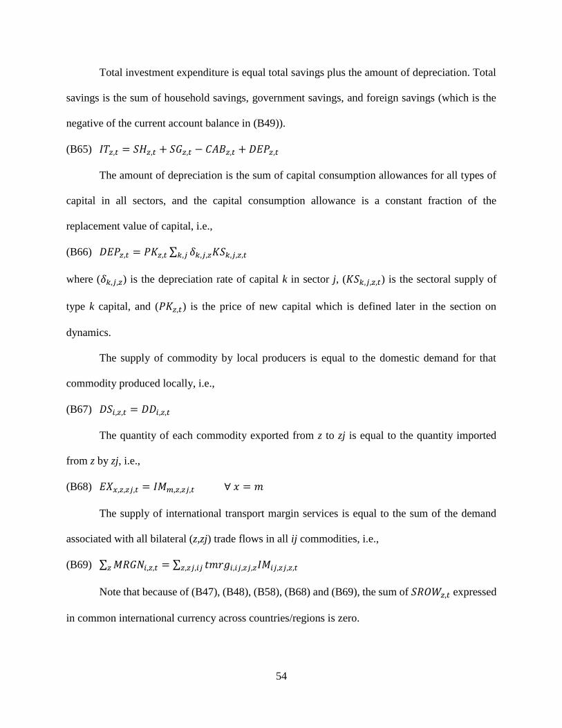
54

Total investment expenditure is equal total savings plus the amount of depreciation. Total

savings is the sum of household savings, government savings, and foreign savings (which is the

negative of the current account balance in (B49)).

(B65) 𝐼𝑇𝑧,𝑡 = 𝑆𝐻𝑧,𝑡 + 𝑆𝐺𝑧,𝑡 − 𝐶𝐴𝐵𝑧,𝑡 + 𝐷𝐸𝑃𝑧,𝑡

The amount of depreciation is the sum of capital consumption allowances for all types of

capital in all sectors, and the capital consumption allowance is a constant fraction of the

replacement value of capital, i.e.,

(B66) 𝐷𝐸𝑃𝑧,𝑡 = 𝑃𝐾𝑧,𝑡 ∑ 𝛿𝑘,𝑗,𝑧𝐾𝑆𝑘,𝑗,𝑧,𝑡𝑘,𝑗

where (𝛿𝑘,𝑗,𝑧) is the depreciation rate of capital k in sector j, (𝐾𝑆𝑘,𝑗,𝑧,𝑡) is the sectoral supply of

type k capital, and (𝑃𝐾𝑧,𝑡) is the price of new capital which is defined later in the section on

dynamics.

The supply of commodity by local producers is equal to the domestic demand for that

commodity produced locally, i.e.,

(B67) 𝐷𝑆𝑖,𝑧,𝑡 = 𝐷𝐷𝑖,𝑧,𝑡

The quantity of each commodity exported from z to zj is equal to the quantity imported

from z by zj, i.e.,

(B68) 𝐸𝑋𝑥,𝑧,𝑧𝑗,𝑡 = 𝐼𝑀𝑚,𝑧,𝑧𝑗,𝑡 ∀ 𝑥 = 𝑚

The supply of international transport margin services is equal to the sum of the demand

associated with all bilateral (z,zj) trade flows in all ij commodities, i.e.,

(B69) ∑ 𝑀𝑅𝐺𝑁𝑖,𝑧,𝑡 = ∑ 𝑡𝑚𝑟𝑔𝑖,𝑖𝑗,𝑧𝑗,𝑧𝐼𝑀𝑖𝑗,𝑧𝑗,𝑧,𝑡𝑧,𝑧𝑗,𝑖𝑗𝑧

Note that because of (B47), (B48), (B58), (B68) and (B69), the sum of 𝑆𝑅𝑂𝑊𝑧,𝑡 expressed

in common international currency across countries/regions is zero.

55

The product market equilibrium where supply is equal to demand for each commodity in

the domestic market of each country/region is defined as

(B70) 𝑄𝑖−1,𝑧,𝑡 = 𝐶𝑖−1,𝑧,𝑡 + 𝐶𝐺𝑖−1,𝑧,𝑡 + 𝐼𝑁𝑉𝑖−1,𝑧,𝑡 + 𝐷𝐼𝑇𝑖−1,𝑧,𝑡

Note that because of Walras Law, one of the demand-supply product equilibrium

conditions is redundant. Thus, (B70) is over (i-1) only.

Gross Domestic Product

The gross domestic product at basic prices (𝐺𝐷𝑃𝑧,𝑡𝐵𝑃) of each country/region is defined as

the payments to factors plus taxes on production but excluding taxes on factors, i.e.,

(B71) 𝐺𝐷𝑃𝑧,𝑡𝐵𝑃 = ∑ 𝑃𝑉𝐴𝑗,𝑧,𝑡𝑉𝐴𝑗,𝑧,𝑡 + 𝑇𝐼𝑃𝑇𝑧,𝑡𝑗

GDP at market price (𝐺𝐷𝑃𝑧,𝑡𝑀𝑃) is GDP at basic prices plus taxes on products and imports,

i.e.,

(B72) 𝐺𝐷𝑃𝑧,𝑡𝑀𝑃 = 𝐺𝐷𝑃𝑧,𝑡

𝐵𝑃 + 𝑇𝑃𝑅𝐶𝑇𝑆𝑧,𝑡

Model Closure

The present global CGE model adopts the PEP-w-t model closure with the following

features:

(a) The numeraire is the GDP deflator of the reference country/region (𝑃𝐼𝑋𝐺𝐷𝑃𝑧𝑟,𝑡), where zr

is the reference country/region. In the present case, zr = NAFTA. In the PEP-w-t model zr

= United States.

(b) Government expenditure in real terms (𝑅𝐺𝑧,𝑡) in (B31) is fixed in each period t in each

country/region.

(c) Public capital investment (𝐼𝑁𝐷𝑘=𝑐𝑎𝑝𝑖𝑡𝑎𝑙,𝑗=𝑔𝑜𝑣𝑟𝑛𝑚𝑒𝑛𝑡,𝑧,𝑡) is fixed in each period t in each

country/region.

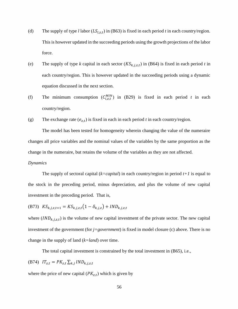
56

(d) The supply of type l labor (𝐿𝑆𝑙,𝑧,𝑡) in (B63) is fixed in each period t in each country/region.

This is however updated in the succeeding periods using the growth projections of the labor

force.

(e) The supply of type k capital in each sector (𝐾𝑆𝑘,𝑗,𝑧,𝑡) in (B64) is fixed in each period t in

each country/region. This is however updated in the succeeding periods using a dynamic

equation discussed in the next section.

(f) The minimum consumption (𝐶𝑖,𝑧,𝑡𝑀𝐼𝑁) in (B29) is fixed in each period t in each

country/region.

(g) The exchange rate (𝑒𝑧,𝑡) is fixed in each in each period t in each country/region.

The model has been tested for homogeneity wherein changing the value of the numeraire

changes all price variables and the nominal values of the variables by the same proportion as the

change in the numeraire, but retains the volume of the variables as they are not affected.

Dynamics

The supply of sectoral capital (k=capital) in each country/region in period t+1 is equal to

the stock in the preceding period, minus depreciation, and plus the volume of new capital

investment in the preceding period. That is,

(B73) 𝐾𝑆𝑘,𝑗,𝑧,𝑡+1 = 𝐾𝑆𝑘,𝑗,𝑧,𝑡(1 − 𝛿𝑘,𝑗,𝑧) + 𝐼𝑁𝐷𝑘,𝑗,𝑧,𝑡

where (𝐼𝑁𝐷𝑘,𝑗,𝑧,𝑡) is the volume of new capital investment of the private sector. The new capital

investment of the government (for j=government) is fixed in model closure (c) above. There is no

change in the supply of land (k=land) over time.

The total capital investment is constrained by the total investment in (B65), i.e.,

(B74) 𝐼𝑇𝑧,𝑡 = 𝑃𝐾𝑧,𝑡 ∑ 𝐼𝑁𝐷𝑘,𝑗,𝑧,𝑡𝑘,𝑗

where the price of new capital (𝑃𝐾𝑧,𝑡) which is given by

57

(B75) 𝑃𝐾𝑧,𝑡 = (1

𝐴𝑧𝐾) ∏ (

𝑃𝐶𝑖,𝑧,𝑡

𝛾𝑖,𝑧𝐼𝑁𝑉 )

𝛾𝑖,𝑧𝐼𝑁𝑉

𝑖

where (𝐴𝑧𝐾) is a scale parameter.

Following Jung and Thorbecke (2001) the sectoral capital investment of the private sector

(j=private) is patterned after the specification of the Tobin’s q. That is,

(B76) 𝐼𝑁𝐷𝑘,𝑗,𝑧,𝑡 = ∅𝑘,𝑗,𝑧 (𝑅𝑘,𝑗,𝑧,𝑡

𝑈𝑘,𝑗,𝑧,𝑡)

𝜎𝑘,𝑗,𝑧𝐼𝑁𝐶

𝐾𝑆𝑘,𝑗,𝑧,𝑡

where (𝑈𝑘,𝑗,𝑧,𝑡) is user cost of type k capital in sector j, (𝜎𝑘,𝑗,𝑧𝐼𝑁𝐶 ) is the elasticity of investment

demand relative to Tobin’s q. The user cost of capita is given as

(B77) 𝑈𝑘,𝑗,𝑧,𝑡 = 𝑃𝐾𝑧,𝑡(𝛿𝑘,𝑗,𝑧 + 𝐼𝑅𝑗,𝑧,𝑡)

where (𝐼𝑅𝑗,𝑧,𝑡) is the interest rate in z in period t. This interest rate is a rationing device that adjusts

so as to satisfy the investment constraint in (B74).

Baseline Scenario

The standard reference scenario is called the ‘business as usual (BaU)’ scenario. This

scenario is generated using the individual countries/regions projections on population (from the

population projections of the United Nations) and on GDP per capita (from the GDP growth

projections of the World Bank). The growth of the per capita GDP (𝑔𝑟𝑧,𝑡

𝐺𝐷𝑃𝑝𝑐) is

(B78) 𝑔𝑟𝑧,𝑡

𝐺𝐷𝑃𝑝𝑐 =𝑔𝑟𝑧,𝑡

𝐺𝐷𝑃+1

𝑔𝑟𝑧,𝑡𝑝𝑜𝑝

+1− 1

where (𝑔𝑟𝑧,𝑡𝐺𝐷𝑃) is the growth rate of GDP, and (𝑔𝑟𝑧,𝑡

𝑝𝑜𝑝) is the growth rate of the population.

Following the PEP-w-t model, some variables and parameters are updated using an index

that incorporates the growth projections of the population and GDP. This index is

(B79) 𝑔𝑑𝑝𝑖𝑛𝑑𝑒𝑥𝑧,𝑡 = (1 + 𝑔𝑟𝑧,𝑡𝑝𝑜𝑝)(1 + 𝑔𝑟𝑧

𝐺𝐷𝑃̅̅ ̅̅ ̅̅ ̅̅ ̅)𝑔𝑑𝑝𝑖𝑛𝑑𝑒𝑥𝑧,𝑡−1, 𝑤𝑖𝑡ℎ 𝑔𝑑𝑝𝑖𝑛𝑑𝑒𝑥𝑧,𝑡=1 = 1

where ( 𝑔𝑟𝑧𝐺𝐷𝑃̅̅ ̅̅ ̅̅ ̅̅ ̅) is defined as

58

(B80) 𝑔𝑟𝑧𝐺𝐷𝑃̅̅ ̅̅ ̅̅ ̅̅ ̅ = (

1

𝑇𝑇−𝑡=1) (∑ 𝑔𝑟𝑧,𝑡

𝐺𝐷𝑃𝑝𝑐𝑇𝑇−1𝑡=1 )

where t=1 is the first period and TT the last period. This index (𝑔𝑑𝑝𝑖𝑛𝑑𝑒𝑥𝑧,𝑡) is used to update the

following variables: 𝐶𝑖,𝑧,𝑡𝑀𝐼𝑁 in (B29), 𝐿𝑆𝑙,𝑧,𝑡 in (B63), 𝐼𝑁𝐷𝑘=𝑐𝑎𝑝𝑖𝑡𝑎𝑙,𝑗=𝑔𝑜𝑣𝑟𝑛𝑚𝑒𝑛𝑡,𝑧,𝑡 in item (c) of the

model closure, 𝑠ℎ0𝑧,𝑡 in (B15), 𝑡𝑡𝑑ℎ0𝑧,𝑡 in (B17), and 𝑅𝐺𝑧,𝑡 in (B31).

Similar to PEP-w-t, the model can be solved so the value of the GDP of each country/region

align with the GDP projections of the World Bank. This is done by setting (𝑔𝑟𝑧,𝑡𝐺𝐷𝑃) equal to the

World Bank projections and solving for a multifactor productivity factor (𝐴𝑧,𝑡𝑉𝐴) for each

country/region over the simulation period (from t=1 to TT). The solution of the model using these

values of (𝐴𝑧,𝑡𝑉𝐴) will generate the GDP growth projections of the World Bank.

Elasticity of Substitution

(a) Between Domestic Products and Imports, and Among Imports of Origin

The elasticity of substitution between domestically produced commodities and imports (in

the first nest in the CES structure in (B41), (B42), and (B43)) is

(B81) 𝜎1𝑚,𝑧 = ∑ 𝑠ℎ𝑖,𝑚,𝑧𝑄

𝑖 𝐸𝑆𝑈𝐵𝐷𝑖

where (𝐸𝑆𝑈𝐵𝐷𝑖) is the elasticity parameter in the GTAP model, and (𝑠ℎ𝑖,𝑚,𝑧𝑄

) is share of sector i

in the base aggregate composite commodities (∑ 𝑄𝑚,𝑧0

𝑚 ) in each country/region. The value of the

elasticity of substitution among imports from the different trading partners (in the second nest in

the CES structure in (B44) and (B45)) is 𝜎2𝑚,𝑧 = 2 ∗ 𝜎1𝑚,𝑧.

(b) Between Factors of Production

The elasticity of substitution between the composite labor and composite capital (the first

nest in the CES structure in (B3), (B4), and (B5)) is

(B82) 𝜎𝑉𝐴,𝑗,𝑧 = ∑ 𝑠ℎ𝑗,𝑧𝑉𝐴

𝑗 𝐸𝑆𝑈𝐵𝑉𝐴𝑗

59

where (𝐸𝑆𝑈𝐵𝑉𝐴𝑖) is the elasticity parameter in the GTAP model, and (𝑠ℎ𝑗,𝑧𝑉𝐴) is share of sector j

in the base aggregate value added (∑ 𝑉𝐴𝑗,𝑧0

𝑗 ) in each country/region. The value of the elasticity of

substitution between the two types of labor (the second nest in the CES structure in (B6) and (B7))

is 𝜎𝐿𝐷,𝑗,𝑧 = 2 ∗ 𝜎𝑉𝐴,𝑗,𝑧. Similarly, the value of the elasticity of substitution between the two types

of capital (the second nest in the CES structure in (B8) and (B9)) is 𝜎𝐾𝐷,𝑗,𝑧 = 2 ∗ 𝜎𝑉𝐴,𝑗,𝑧.

(c) Between Domestic Market and Exports, and Among Export Destination

The elasticity of transformation in the first nest of the CET structure (B34), (B35), and

(B36) is 𝜎1𝑥,𝑧 = 2, while in the second nest in (B38), and (B39) is 𝜎2𝑥,𝑧 = 3.

The welfare measure used in the analysis is equivalent variation (EV). The global model

used in the analysis utilizes a LES system whose demand functions are given in (B29). Robichaud

(2001) has shown that the EV corresponding to a demand system which is LES may be written as

(B83) 𝐸𝑉𝑧,𝑡 = ∏ (𝑃𝐶𝑖,𝑧,𝑡

𝐵

𝑃𝐶𝑖,𝑧,𝑡𝑆 )

𝑔𝑎𝑚𝑚𝑎_𝐿𝐸𝑆𝑖,𝑧

(𝐶𝑇𝐻𝑧,𝑡𝑆 − ∑ 𝐶𝑀𝐼𝑁𝑖,𝑧,𝑡

𝐵𝑖 𝑃𝐶𝑖,𝑧,𝑡

𝑆 )𝑖 − (𝐶𝑇𝐻𝑧,𝑡𝐵 −

∑ 𝐶𝑀𝐼𝑁𝑖,𝑧,𝑡𝐵

𝑖 𝑃𝐶𝑖,𝑧,𝑡𝐵 )

where the superscript B refers to the baseline solution, while S to the simulation solution.

60

Appendix C: Philippine Poverty and Income Distribution Simulation Model

The FIES provides information on household income. Household income is composed of

labor income (total wages and salaries, which is further divided into wages and salaries from

agriculture and non-agriculture) and all other income (which includes net share of crops, income

from entrepreneurial activities, remittances, etc.). Let the total household income be

(C1) 𝑌ℎ = 𝑤 ∙ 𝐿 + 𝑟 ∙ 𝑂𝑌

where Yh is total household income, w wage rate, L labor, rate of return or payment to other income,

OY. w and r are factor prices while L and OY are factor endowments of households, which include

income from land ownership. In the poverty microsimulation model, the results from the CGE

simulation are used to change w, L, and r to determine the change in Yh.

The poverty threshold can be specified as

(C2) 𝑃𝑜𝑣∗ = 𝑃 ∙ 𝑀𝐵𝑁

where Pov* is value of the poverty threshold, P commodity prices, and MBN the minimum basic

needs. The value of the poverty thresholds changes with changes in commodity prices. Changes

in commodity prices are taken from the CGE simulation results. MBN is held fixed.

Consider a situation where a certain household is initially below poverty, i.e., Yh < Pov*.

Changes in w, r, L and P as a result of the implementation of the NGP could lead to a situation

where the household could either remain in poverty (i.e. Yh < Pov*) or move up the poverty

threshold (Yh > Pov*). This is poverty analysis is conducted in the project. In addition, since Yh

changes across households, the distribution of income also changes. This is also analyzed in the

project. These effects across households are analyzed using the poverty microsimulation model

that utilizes data from the FIES. The FIES provides several household information including

61

job/business indicator for the household heads, occupation, as well as employment status

(employed/unemployed).

Based on the FIES, households can be grouped into those whose household heads are

unemployed and those with employment. This is illustrated in Figure 2 below as the employment

bar divided into two parts by a line7. Those above the line are employed, while those below are

unemployed. Employed household heads earn labor income, while those who are unemployed do

not.

Poverty Microsimulation

A CGE policy simulation generates changes in sectoral employment, factor prices (wages,

returns to capital, and returns to land), and commodity prices. These results are used to change the

7 Detailed discussion of the poverty microsimulation is give in Cororaton, C. B., and E. Corong. 2009. Philippine

Agricultural and Food Policies: Implications on Poverty and Income Distribution. International Food Policy Research

Institute (IFPRI) Research Report No. 161. Washington DC: IFPRI.

62

employment bar in the figure shown. To illustrate, assume the employment bar represents

employment in agriculture. Assume a CGE policy shock generates a relative sectoral price ratio

that favors agriculture. Since agriculture is profitable relative to industry and services, assuming

fixed supply of resources (labor, capital, and land), some of the resources used in industry and

services will move to agriculture, thereby increasing the output of the agricultural sector. The

demand for labor in agriculture will increase, as well as the demand for other factor inputs.

Higher employment in agriculture will move the employment bar in agriculture up as

shown in the figure in the post CGE simulation. The number of unemployed in agriculture will

decline (those below the horizontal line), while the number of employed will expand (those above

the line). The change in agricultural employment from the CGE simulation will determine how far

the employment bar is shifted upwards.

There is an area in the employment bar (Area E) which represents those who were

originally unemployed during the pre-CGE simulation but have gained employment in the post-

CGE simulation. The question then is: how does one select who among the unemployed household

heads during the pre-CGE simulation will gain employment in the post-CGE simulation? In the

poverty microsimulation model, the previously unemployed household heads in Area E are

randomly selected from a pool of unemployed household heads in the pre-CGE simulation. Once

they are selected and included in Area E, they are assigned a wage, w, which is determined from

the CGE simulation. As a results, these household heads will start generating labor income which

will increase their total household income.

The random selection of unemployed household heads is repeated for 30 times. In each

repeated random selection of household heads, the composition of households in Area E is

different. In each repeated random selection, poverty indices and income distribution coefficient

63

are calculated. This repeated random selection will allow one to establish confidence interval of

the estimates of the poverty indices and the income distribution coefficient.

Conversely, the same process is applied to household heads who belong to the contracting

sectors, industry and services. Unemployment in these sectors will increase and some of the

employed household heads will get unemployed and will lose labor income. The random selection

of the employed household heads is also done for 30 times to establish confidence intervals for the

estimates of the poverty indices and income distribution coefficient.

In the project, the Foster-Greer-Thorbecke (FGT) poverty indices (see below for the

formula) are computed using data in the FIES data. The income distribution coefficient that will

be used is the GINI coefficient. The FGT indices and the GINI coefficient are computed separately

during the pre-CGE simulation and in the post-CGE simulation. The results are then compared to

determine whether the NGP generates favorable poverty and distributional impacts or not.

FGT Poverty Indices. The simplest measurement of poverty, for a given poverty line, is to

assess how many households or individuals fall below that line. Expressed as a proportion of the

whole population this constitutes the poverty headcount ratio (P0). However, this measure

overlooks how intense household’s poverty is, and for instance does not differentiate between a

household living just below the poverty line and another far below. A common measure to account

for the intensity of poverty is the poverty gap (P1), which measures the average distance of poor

households from the poverty line. Finally, a third measure is used to capture poverty severity index

(P2) which captures the degree of inequality amongst the poor. All three measures are specific

measures of the generalized FGT poverty metric, where alpha equals 0, 1 and 2 respectively.

(C3) 𝑃𝛼 =1

𝑁∑ (

𝑧−𝑦𝑖

𝑧)𝛼𝐻

𝑖=1

64

There are several ways of measuring inequality. The most common is through the GINI

ratio, which measures the area between the 450 perfect equality line and the Lorenz Curve. The

value of the coefficient ranges between 0 (perfect equality) and 1 (complete inequality). This

measurement of inequality is used in the project. The formula of the GINI coefficient is given by

(C4) 𝐺𝐼𝑁𝐼 =1

2𝑛2�̅�∑ ∑ |𝑦𝑖 − 𝑦𝑗|𝑛

𝑗=1𝑛𝑖=1

where n is the number of individuals, yi and yj are income of the individuals, and �̅� is the mean

income.

The step-by-step procedure given below adopts some features of the process in Vos (2005).

1. The household head represents the entire family. In the first phase of this procedure,

household heads are distinguished by: (a) skill level; and (b) sector of employment. Sector of

employment is differentiated into agriculture and non-agriculture whereas skill level is classified

into unskilled (no education to non-high school graduates) and skilled (high school graduates and

higher). There are 4 labor income sources/sectoral employment groups: unskilled agriculture,

skilled agriculture, unskilled non-agriculture, and skilled non-agriculture.

2. Generate a dummy variable called employed where 1 = households with wage income and

zero otherwise. Compute the total employment rate u*for each of the four groups defined in step

5. The total employment rate for each group, u* is the weighted mean of the dummy variable

employed and weights in the household survey. Note that the dummy variable is only a subset of

the survey as it only covers those with wage income (dummy variable =1) and those with zero

wage income but unemployed (dummy variable = 0).

3. Update the total sectoral employment u*in the household survey by using the variation in

sectoral employment from the CGE model.

65

4. Assign a random number from a normal distribution to those identified as employed. This

is called random. The variables random and employed are then sorted by descending order.

5. Compute the accumulated weight of employed in each group (by sector and by skill level

as defined in 5).

6. Compute the over-all weight of each group. This is simply the sum of accumulated weight

by sector and by skill level as defined in 5.

7. Take the ratio of accumulated weight and the overall weight of each group. This ratio is

called rij.

8. Compare rijand u*. If rij ≤ u*, then that household head is employed, and unemployed

otherwise (rij> u*).

9. Arrange each group in decile. The decile grouping is based on the sum of labor income and

capital income, where capital income is the sum of ‘total income from entrepreneurial activities’

and ‘net share of crops’ in the household survey. Other incomes such as dividends, interest income

and others are not used in grouping households into decile.

10. Assign the decile mean labor income to those who become newly employed (after a change

in u*), and reduce labor income of those who become unemployed8 (after a change in u*,). For

those who become newly employed, and if they belong to the first decile for example, the mean

labor income in the first decile will be assigned to them. Those with labor income, but not picked

by the random process will retain their labor income. On the other hand, those with zero labor

income but not picked by the random process will continue to have no labor income earnings.

8 In reducing labor income of those who become unemployed, that is, they will move to the area where rij> u*after

the change in u*. The one we adopted involves deducting the decile mean labor income from the labor income if the

former is less than the latter. Otherwise, labor income is reduced to zero.

66

11. Define total income. It is composed of three major items: labor income, capital income,

and other income. Capital income is income derived from the various production sectors other than

labor income, while other income includes income from dividends, government transfers, and

remittances. Note that similar income sources are found in the CGE model and in the household

survey.

12. Derive the change in capital and other income of each household in the survey using the

average change in capital and other income per household category from the CGE model.

13. Derive the change in labor income in a two-step procedure: (a) use the change in labor

income of each household in the survey from the average change in labor income per household

category from the CGE model; (b) update the final labor income using the result of the random

process carried in step 8.

14. Compute for the total household income by taking the sum of labor income, capital income,

and other income.

15. Update the nominal value of the poverty line of each household in the survey by applying

the variation in household specific consumer price index from the CGE model.

16. Calculate the GINI coefficient using the new column of income, as well as the FGT poverty

indices using the income and new nominal poverty line.

17. The FGT poverty indices are calculated according to the demographic characteristics of

the household head: (1) gender; (2) skill level; and (3) location, urban-rural. In total, the final FGT

indices are derived for households both in decile and socio-economic categories. The micro-

simulation process is repeated 30 times9. Thus, there will be 30 estimates of GINI coefficient and

9 Vos (2005) observes that 30 iterations are sufficient. Repeating this process additionally does not significantly alter

the results.

67

FGT indices in each simulation. Confidence intervals of estimates from the 30 simulations/runs

are derived.