Potential benefits from data assimilation of carbon observations for modellers and

observers - prerequisites and current state

J. Segschneider, Max-Planck-Institute for Meteorology, Hamburg

WP 1: Prediction towards sustainable development

with input from B. Pfeil (UiB), C.Heinze(UiB)

directly linked WPs: 6, 11

why data assimilation?

data assimilation is the general term for the combination of models and observations. it can

be used to

• fill gaps in data sets• identify errors in models and observations• optimize initial conditions for future projections

can data assimilation fill gaps in observational data sets?

• in principle: yes

• examples: SST maps, sea level from altimeter maps

two basic approaches:

• dynamic interpolation ( use a model to spread the

information in space/time)

• statistical/optimal interpolation (requires definition of

observation error to provide weights in a least squares fit

and the definition of a radius of information in space and

time)

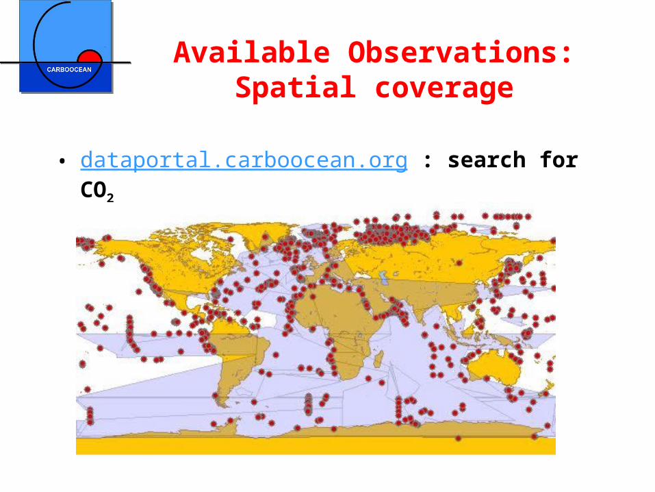
Available Observations: Spatial coverage

• dataportal.carboocean.org : search for CO2

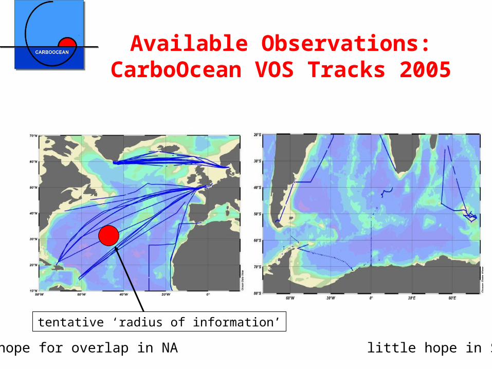
tentative ‘radius of information’

some hope for overlap in NA little hope in SA/I

Available Observations: CarboOcean VOS Tracks 2005

Quality control in the context of data assimilation

• do the observations represent scales that the models can resolve (‘null space’)?

• are neighbouring observations consistent? • for which time window are the observations

valid?• observation error usually determined by standard

deviation of data (as a whole), but different data sources could have different weights if instrumental errors are known

• whole work field in itself

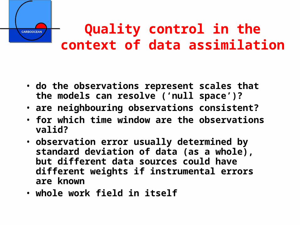
Quality control in the context of data assimilation

• do the observations represent scales that the models can resolve (‘null space’)?

• are neighbouring observations consistent? • for which time window are the observations

valid?• observation error usually determined by standard

deviation of data (as a whole), but different data sources could have different weights if instrumental errors are known

• whole work field in itself

can we use data assimilation to optimize our initial conditions for

climate projections?

The general problem of state estimation

• numerical models have errors B (background error)

• forcing fields have errors B

• observations have errors R (observation error)

the ‘true’ state is not known

• but: initial conditions impact on predictions

• The task is, to optimally combine models and observations

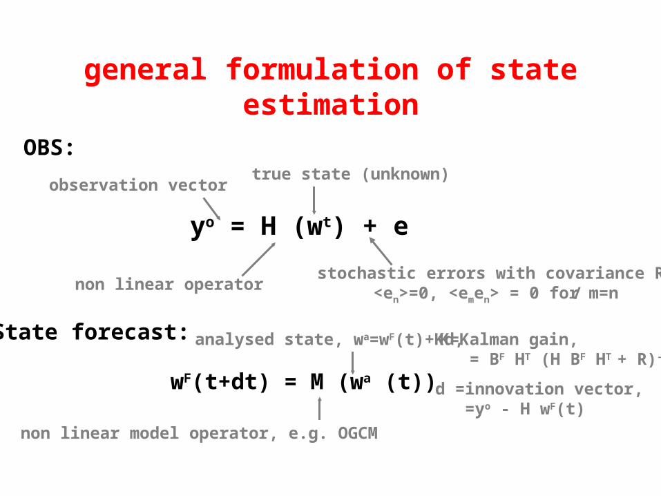
general formulation of state estimation

yo = H (wt) + e

stochastic errors with covariance R,<en>=0, <emen> = 0 for m=n

observation vectortrue state (unknown)

non linear operator

OBS:

State forecast:

wF(t+dt) = M (wa (t))

non linear model operator, e.g. OGCM

analysed state, wa=wF(t)+Kd, K=Kalman gain, = BF HT (H BF HT + R)-1

d =innovation vector, =yo - H wF(t)

/

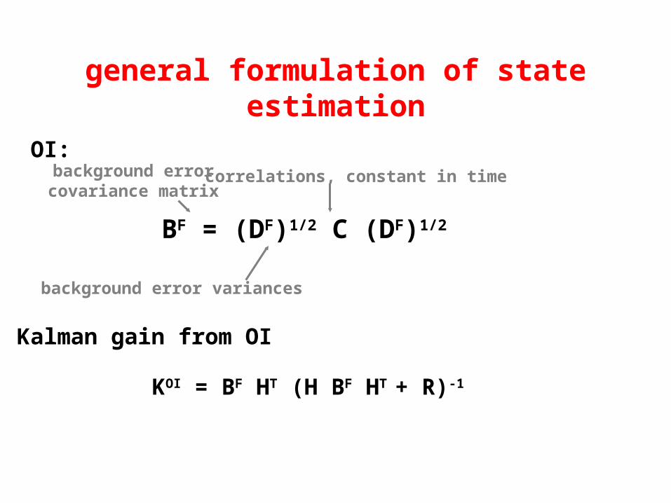
general formulation of state estimation

BF = (DF)1/2 C (DF)1/2

background errorcovariance matrix

correlations, constant in time

background error variances

OI:

Kalman gain from OI

KOI = BF HT (H BF HT + R)-1

Analysis cycle

time. observed state at time t [t-tobs/2, t+tobs/2]

simulated state (background, first guess)x

state vector

.x

+.x+.x+

.x

+

.x+

.x

+

+ analysis, xt = f (xt-1,wt-1, (, Q, P-E[t-1,t]))

analysis incrementw

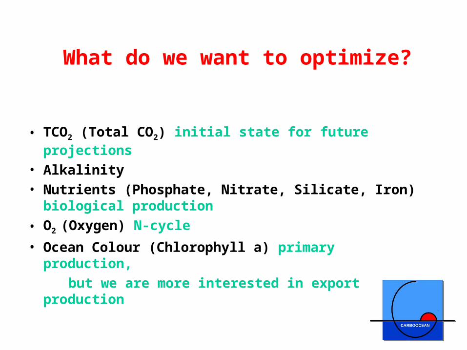
What do we want to optimize?

• TCO2 (Total CO2) initial state for future projections

• Alkalinity • Nutrients (Phosphate, Nitrate, Silicate, Iron)

biological production

• O2 (Oxygen) N-cycle

• Ocean Colour (Chlorophyll a) primary production,

but we are more interested in export production

www.ncof.gov.uk

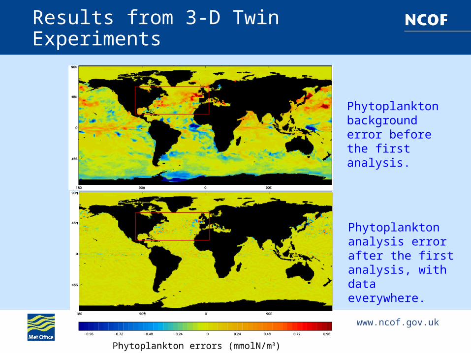
Phytoplankton background error before the first analysis.

Phytoplanktonanalysis error after the first analysis, with data everywhere.

Phytoplankton errors (mmolN/m3)

Results from 3-D Twin Experiments

www.ncof.gov.uk

Daily mean RMS Errors in the North Atlantic

Total Dissolved Inorganic Carbon (mmolC/m3)

Control - truth

Assimilation - truth

Results from 3-D Twin Experiments

Potential specifications of an operational carbon cycle analysis

system

• A relatively simple assimilation scheme like multivariate OI should do. (but we could learn more from 4dVAR -- AWI: adjoint -- WP6)

• Seasonal or even annual averages will suffice for most purposes – no ‘near real time’ issues but test within PIRATA buoy array (Atlantic)

• How to define background and observation errors?

• Manual quality control or automatic?• One or more carbon cycle models?

Potential Analysis Systems - Variables and WPs

• Sea Surface + in-situ Temperature, Salinity

• Total CO2 , alkalinity (WP8)

• Oxygen (WP 4)

• CO2 flux atmosphere – ocean (WPs 5,6)

• Ocean colour (WP 6)• Gas exchange coefficient (?)

• Cant (?) (WP 9)

Potential Analysis Systems - Requirements

• Automatic data acquisition and quality control• Automized model/assimilation system runs • Control of output quality• Dissemination of analysis to potential users

Conclusion: Not a trivial task!