Posterior Distributions for Welfare Changes in Agricultural

Commodity Markets

Adam Bialowas and William Griffiths

Department of Economics

The University of Melbourne

Victoria 3010, Australia

May 2008

A formal Bayesian-based methodology is presented for evaluating the welfare effects

of economic changes in agricultural commodity markets. The procedure is applied to

an empirical example, demonstrating how posterior densities may be obtained for

estimated welfare changes. These posterior densities provide an intuitive and rigorous

method for illustrating the robustness of the results from an applied welfare analysis

to the effects of parameter uncertainty. The procedure is used to explore the

implications of stochastic error terms in supply and demand curves for the

measurement of welfare changes.

Keywords: Bayesian, welfare analysis, sensitivity analysis

2

1. Introduction

Applied welfare analyses are frequently conducted by agricultural and resource

economists in order to examine a wide variety of issues and problems which are

relevant to the agricultural and resource sector. For instance, following the example

set by Griliches (1958), they have been used extensively to estimate the rates of return

to agricultural research and promotional activities. Similarly, Wallace (1962)

illustrated how applied welfare analyses may be used in a benefit cost framework to

differentiate between alternative policies which have been designed to achieve the

same goal. Subsequent to these early examples, many articles have appeared in the

literature which are either advances, refinements or applications of the concepts used

in these studies.

One such stream of research has been concerned with developing methodologies for

incorporating the effects of parameter uncertainty into applied welfare analyses. This

work has been motivated by the acknowledgement that estimates of the various

measures which may be used in such studies are entirely dependent upon the

parameter values use to calculate them. For instance, estimates for the commonly

used Marshallian welfare measures of consumer and producer surplus are dependent

on the parameters of demand and supply functions. Irrespective of whether these

parameter values have been obtained from econometrically estimated structural

models, previously published estimates, or guided by economic theory and individual

expert opinion, there is uncertainty regarding their true values. Consequently, these

estimates, and by extension, the results and conclusions which may be drawn from

them, are also subject to uncertainty.

This uncertainty has been incorporated into previous studies in different ways. The

most common method is to propose a set of plausible, alternative parameter values,

and then use these values compute the corresponding series of welfare changes.

Examples can be found in Wallace (1962), Harrison and Vinod (1992) and Mullen,

Alston and Wholgenant (1989). This approach provides a quick and simple method

for determining whether apparently small changes in parameter values may lead to

qualitatively different results or conclusions. This basic methodology may be given a

more rigorous footing by specifying subjective probability distributions for the

parameters based on the knowledge of experts, and then using simulation techniques

3

to trace out the implied subjective probability distributions for the welfare changes

themselves as has been done by Abler, Rodrieguez and Shortle (1999), Davis and

Espinoza (1998) and Zhao et al (2000).

Where data has been available, other studies have been able to appeal to the sampling

theory properties of econometrically obtained parameter values to find estimates for

the moments of a particular welfare change estimate. This may be achieved through

the use Taylor’s series approximations to approximate the variance of an estimated

welfare change, which is often a complex nonlinear function of the parameters in the

model (Alston and Larson, 1993; Chotikapanich and Griffiths, 1998). Alternatively,

bootstrapping techniques may be used to determine the statistical properties

associated with an estimate (Kling and Sexton, 1990). Further studies have treated the

sampling distributions of the estimated parameters like a posterior distribution, from

which draws are simulated to estimate welfare changes (Adamowicz, et al., 1989);

Creel and Loomis, 1991).

Bayesian inference provides an alternative methodology for accommodating the

effects of parameter uncertainty in applied welfare analyses. It may be considered to

be an advance on previous approaches in that it explicitly allows for the incorporation

of both sample and non-sample. Consequently, Bayesian inference has been

promoted as providing an ideal framework for accommodating the impacts of

parameter uncertainty in applied welfare analysis (Zhao et al., 2000); Pannell, 1997).

Despite such recommendations however, no such methodology has been thus far been

developed which is suitable for investigating the types of examples relevant to the

agricultural sector. Hence in this paper we present a formal Bayesian-based

methodology for evaluating the welfare effects of economic changes in agricultural

commodity markets.

This methodology may also be extended to allow for the effects of other sources of

uncertainty. For instance, the proposed methodology is dependent upon the

availability of econometrically obtained parameter estimates. Associated with every

econometric model is a stochastic error term which may be interpreted as representing

the predictive uncertainty of the model. Traditional approaches ignore this source of

uncertainty by only considering the deterministic component of an econometric model

when calculating estimates of consumer and producer surplus. However, Bockstael

4

and Strand (1987) provided some results illustrating that the results from an applied

welfare analysis may be affected by the convention taken regarding the error term.

To help illustrate the various elements of this procedure, a simple empirical example

will be used in which the welfare impacts associated with an exogenous demand shift

in the domestic demand for Australian lamb are evaluated. In Section 2 we describe a

2-equation dynamic model for the demand and supply of lamb. Because the model is a

dynamic one, and because we are considering welfare changes that occur when

moving from one equilibrium position to another, we derive expressions for

equilibrium price and quantity. In Section 3 we introduce an exogenous permanent

shock that increases the demand for lamb and we derive expressions for the welfare

changes that result from this increase in demand. In Section 4 we describe how to

estimate posterior densities for the welfare changes given in Section 3. The results

from an empirical illustration are presented in Section 5 and some concluding remarks

given in Section 6.

2. Model

One of the characteristics of the Australian agricultural sector is the various

interrelationships which exist between different commodities in either demand or

supply. In general this has led to the use of multi-equation modelling frameworks,

which explicitly incorporate as many of these relationships as is feasible, when

describing agricultural commodity markets, e.g., Vere, Griffith and Jones (2000).

When conducting an applied welfare analyses, this approach also has the advantage of

providing information on the distribution of welfare effects amongst different groups

following an economic change. To help demonstrate the practicality of the proposed

Bayesian approach, the econometric model of the Australian lamb industry used in the

example to demonstrate this procedure will follow this convention.

The model of the Australian lamb industry in the example consists of two equations

linked in a recursive relationship with a third equation imposing a market clearing

condition. It is given by

(1) 1 2 , 3 4 5

L L B C

t D t t t t tP Q Y Q P d= α + α + α + α + α + ε

(2) , 1 2 1 3 , 1 4 1

L L L

S t t S t t tQ P Q DT s− − −= β + β + β + β + ε

5

(3) , ,

L L

D t S tQ Q=

where

,

L

D tQ = Australian per-capita consumption of lamb in kg

L

tP = The deflated Australian retail price for lamb in c/kg

B

tQ = Australian per-capita consumption of beef in kg

tY = The deflated Australian per capita disposable income in dollars

C

tP = deflated Australian retail price for chicken in c/kg.

,

L

S tQ = Australian per-capita supply of lamb in kg

tDT = Incidence of drought: A dummy variable denoting a drought in period t.

t = index for time

&t t

d sε ε = error terms where ( , ) (0, )t t

d s N′ε ε Σ�

Given the market clearing condition in (3), in what follows we will not distinguish

between quantity demanded and quantity supplied. We will simply write L

tQ ,

dropping the S and D subscripts as well as equation (3).

In equation (2) quantity supplied depends only on previously determined values of

price and quantity as well as the drought incidence variable. It can be viewed as a

partial adjustment model where quantity supplied cannot adjust fully to desired

quantity within one period and where lagged price is a proxy for price expectations.

Then, given quantity supplied depends only on predetermined variables, the demand

curve can be viewed as one where price adjusts to clear the market. Thus, the demand

equation in (1) is written as a price dependent one. Also writing it in this way proves

convenient for later estimation.

The inclusion of income in the demand equation is natural, but the presence of the

quantity of beef and the price of chicken needs more explanation. An increase in the

demand (or supply) of beef will lead to a decrease in the price of lamb. An increase in

the price of chicken will lead to increase in the demand for lamb and hence a higher

lamb price. While it would have been more consistent to include the quantities of both

6

substitute meats instead of the price of chicken, data on the price of chicken was more

readily available, and if one views the equations as a subset of a more complete set of

simultaneous equations, there are a variety of ways in which the effects of price-

quantity changes in the other markets, treated as exogenous for the purpose of this

example, can be represented.

The welfare changes, for which the posterior densities will be obtained, are to be

generated by an exogenous shift in the demand for lamb. Given the dynamic nature

of the supply equation, the effects of such a shift will be felt for several periods and it

will take time to reach a new equilibrium. This observation raises questions about

how consumer and producer surplus change in each time period, about the aggregate

changes over all periods and about the changes when one goes from equilibrium

position to the next. The dynamic welfare changes, how they are defined and

estimated, are described in Bialowas (2007) and will be the subject of another paper.

At this time we focus on a comparison of consumer and producer surpluses at initial

and final equilibrium points.

The first step in this direction is to define equilibrium prices and quantities. To do so

we need to set specific values for the exogenous variables and assume that these

values are constant at these particular values. Using an over-bar to denote these

values, a notation consistent with setting them at the sample means, it is convenient to

redefine the intercepts in the model to include the constant exogenous variables. Thus

we have

(4) 1 1 3 4 5

B

CY Q P

∗α = α + α + α + α

(5) 1 1 4 DT∗β = β + β

Then, the model can be written as

(6) 2 1 1

*2 3 1 1

0 01

0 1

L L

tt t

L Ltt t

dP P

sQ Q

∗−

−

ε−α α − = + β β εβ

Letting

2

0

1

0 1A

−α =

1

2 3

0 0A

= β β

and multiplying through by 1

0A− , equation (6) can be rewritten as

7

(7) 1 1 11 1

0 1 0 0*

1 1

L Ltt t

L L

tt t

dP PA A A A

sQ Q

∗− − −−

−

ε α − = + εβ

or

(8) 1 1 110 1 0 0*

1

( )L

tt

Ltt

dPI A A L A A

sQ

∗− − −

ε α − = + εβ

where L is the lag operator. Solving for price and quantity yields

(9) 1 1 1 1 1 11

0 1 0 0 1 0*

1

( ) ( )L

tt

L

tt

dPI A A A I A A L A

sQ

∗− − − − − −

ε α = − + − εβ

where the lag operator drops out of the first right-hand-side term because 1 1( , )∗ ∗α β is

constant. We use (9) to distinguish between a stochastic equilibrium and a

deterministic equilibrium. The deterministic equilibrium is obtained by ignoring the

error terms. Thus we have

(10) 1 1 1 1

0 1 0 *

1

( )L

DIE

L

DIE

PI A A A

Q

∗− − − α

= − β

where DIE refers to deterministic initial equilibrium, the deterministic equilibrium

before the shift in demand. Letting

(11) 1 1 1 1

0 1 0

2

( )tE

tE

dvI A A L A

sv

− − −ε

= − ε

be a realization of the equilibrium error terms, the stochastic initial equilibrium is

given by

(12) 1

2

L L

ESIE DIE

L L

ESIE DIE

vP P

vQ Q

= +

To complete the specification of this stochastic equilibrium, we need the distribution

of the errors. Given that ( , ) (0, )t t

d s N′ε ε Σ� , it can be shown that

1 2( , ) (0, )E E v

v v N′ Σ� where, given that conditions necessary for the stability of the

model are satisfied, the covariance matrix v

Σ is obtained from

1vec( ) ( ) vec( )v

I B B−Σ = − ⊗ Σ where 1

0 1B A A−=

See, for example, Lütkepohl (1991, p.21).

8

To be able to define consumer and producer surplus at equilibrium prices and

quantities, it is necessary to define equilibrium demand and supply curves consistent

with the equilibrium prices and quantities in equations (10) and (12). Using the

subscript E to denote equilibrium, the equilibrium equations are given by

(13) 1 2

L L

E E EP Q d

∗= α + α + ε

(14) 1 2

L L

E E EQ P w∗= δ + δ +

where 1 1 3/(1 )∗ ∗δ = β −β and 2 2 3/(1 )δ = β − β . The subscript E on the error terms

denotes a realized error at equilibrium. The error E

w is a realization from the

distribution of 1

2 3(1 )t

L s−β −β ε . The deterministic equilibrium values L

DIEP and L

DIEQ in

(10) are given by the simultaneous solution of (13) and (14) with the error terms

ignored. The stochastic equilibrium values L

SIEP and L

SIEQ in (12) are given by the

simultaneous solution of (13) and (14), with appropriate recognition given to the

bivariate distribution for ( , )E E

d w ′ε .

We are now in a position to examine the welfare changes that occur when going from

an initial equilibrium point to a final equilibrium point following a shift in the demand

curve.

3. Welfare effects

The shift in the demand function is represented by a change in the intercept of

equation (2) by an amount equal to k ( 0k > ) units. Thus, the new demand curve

becomes

(15) 1 2 , 3 4 5

L L B C

t D t t t t tP k Q Y Q P d= α + + α + α + α + α + ε

The resulting new deterministic and stochastic equilibrium values, subscripted as DFE

and SFE to denote a final equilibrium, are given by

(16) 1 1 1 10 1 0 *

1

( )L

DFE

L

DFE

P kI A A A

Q

∗− − −

α += −

β

and

9

(17) 1

2

L L

ESFE DFE

L L

ESFE DFE

vP P

vQ Q

= +

The errors in equations (12) and (17) are assumed to be the same. Thus, we are

comparing two hypothetical equilibrium points where the demand is greater in one

than the other, but the realized error terms are the same for each scenario. The new

equilibrium demand equation obtained by modifying (13) is

(18) 1 2

L L

E E EP k Q d∗= α + + α + ε

The equilibrium supply equation remains the same as (14). The deterministic

equilibrium values L

DFEP and L

DFEQ in (16) are given by the simultaneous solution of

(18) and (14) with the error terms ignored. The stochastic equilibrium values L

SFEP and

L

SFEQ in (17) are given by the simultaneous solution of (18) and (14) with due

recognition of the error terms.

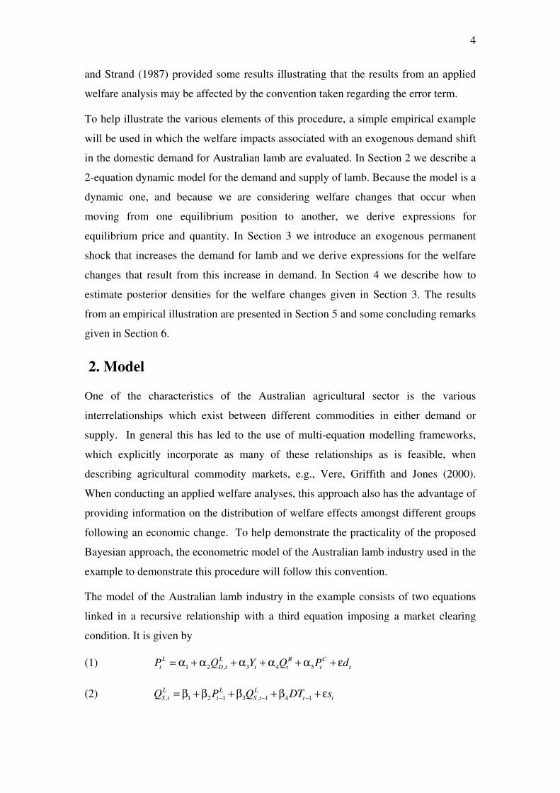
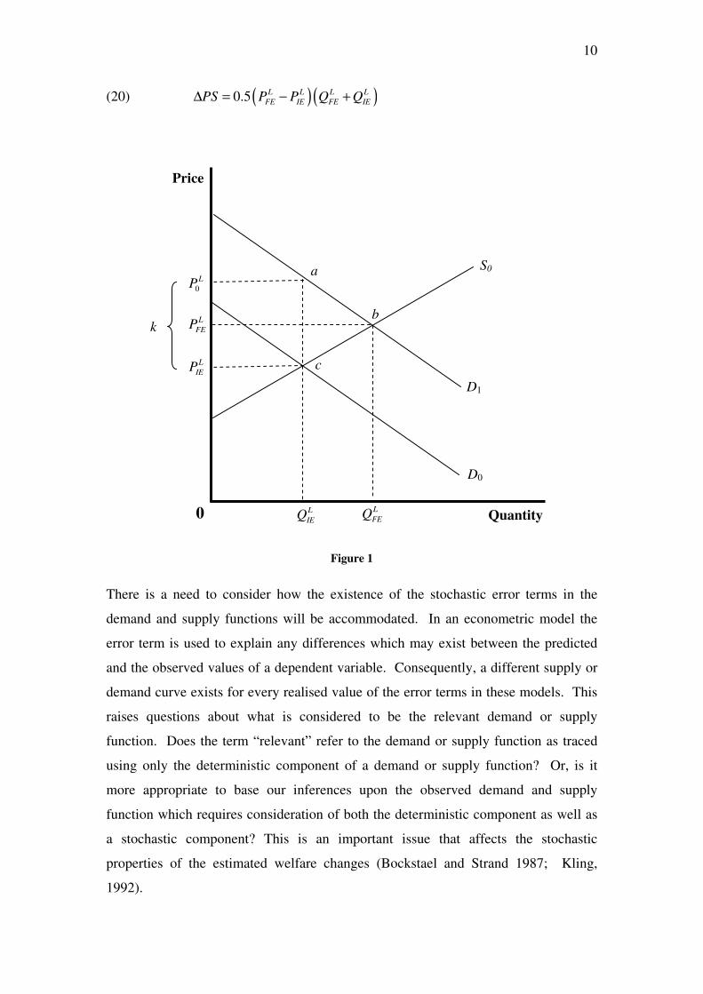
The effects of the proposed demand shock may be illustrated diagrammatically using

Figure 1. The demand equations in (13) and (18) are represented by 0D and 1D ,

respectively; the supply equation in (14) is denoted by 0S . Abstracting for the

moment from the question of deterministic versus stochastic equilibrium, the effect of

the demand shock is to shift the demand function vertically along the price axis by an

amount equal to k, to increase equilibrium quantity from L

IEQ to L

FEQ and to increase

equilibrium price from L

IEP to L

FEP .

When defining the welfare changes caused by the demand shift the Marshallian

welfare measures of consumer and producer surplus will be used. These welfare

measures are frequently conceptualised as geometric areas behind demand and supply

curves. For instance, in the current example, the change in consumer surplus resulting

from the demand shift may be represented geometrically as the area 0

L L

FEP abP behind

the demand curve 1D , where 0

0

L

FEP P k= + . Similarly, the change in producer surplus

resulting from the demand shift is represented by the trapezoidal area L L

FE IEP bcP behind

the supply function S0. In terms of equilibrium prices and quantities, these quantities

are

(19) ( )0.5( )L L L L

IE FE FE IECS P k P Q Q∆ = + − +

10

(20) ( )( )0.5 L L L L

FE IE FE IEPS P P Q Q∆ = − +

Figure 1

There is a need to consider how the existence of the stochastic error terms in the

demand and supply functions will be accommodated. In an econometric model the

error term is used to explain any differences which may exist between the predicted

and the observed values of a dependent variable. Consequently, a different supply or

demand curve exists for every realised value of the error terms in these models. This

raises questions about what is considered to be the relevant demand or supply

function. Does the term “relevant” refer to the demand or supply function as traced

using only the deterministic component of a demand or supply function? Or, is it

more appropriate to base our inferences upon the observed demand and supply

function which requires consideration of both the deterministic component as well as

a stochastic component? This is an important issue that affects the stochastic

properties of the estimated welfare changes (Bockstael and Strand 1987; Kling,

1992).

D1

S0

L

FEP

L

IEP

L

FEQ L

IEQ0 Quantity

Price

k

D0

c

a

b

0

LP

11

In the first approach that we adopt only the deterministic components of the demand

and supply functions are considered when deriving algebraic expressions for the

changes in consumer and producer surplus. The premise for this approach is that,

should the same exogenous shift to be repeated at different times, there would be

different realisations for the errors. On average however, these realisations will

average out to zero and only the welfare estimate which corresponds to this value for

the error is considered to be of interest. For this reason, under this approach the

welfare changes may be interpreted as a long-run effect.

Expressions derived under this approach will be called deterministic changes in

consumer and producer surplus. Including the subscript D to denote deterministic,

these changes are given by

(21) ( )0.5( )L L L L

D DIE DFE DFE DIECS P k P Q Q∆ = + − +

(22) ( )( )0.5 L L L L

D DFE DIE DFE DIEPS P P Q Q∆ = − +

The objective of this study is to show how to derive posterior densities for these

changes and hence provide a means for expressing the uncertainty associated with

estimating these quantities. Assuming the model specification is correct, when

deterministic quantities are used, the only source of uncertainty in (21) and (22) will

be the unknown parameters in the supply and demand curves. However, realized

prices and quantities depend on realized error terms. Thus, it seems reasonable to also

consider the uncertainty associated with the error terms when deriving the posterior

densities of the changes in consumer and producer surplus. To describe the surplus

changes that include error uncertainty we use the subscript S, recognizing that these

changes are stochastic. They are given by

(23)

( )( )

( )( ) ( )

( )

2

2

0.5

0.5

L L L L

S SIE SFE SFE SIE

L L L L L L

DIE DFE DFE DIE DIE DFE E

L L

D DIE DFE E

CS P k P Q Q

P k P Q Q P k P v

CS P k P v

∆ = + − +

= + − + + + −

= ∆ + + −

(24)

( )( )

( ) ( )

( )

2

2

0.5

0.5

L L L L

S SFE SIE SFE SIE

L L L L

DFE DIE DFE DIE E

L L

D DFE DIE E

PS P P Q Q

P P P P v

PS P P v

∆ = − +

= − + −

= ∆ + −

12

Having derived algebraic expressions for the welfare changes resulting from the

demand shift, the next step in the procedure involves deriving Bayesian posterior

densities for the parameters in the model. The deterministic changes in welfare

depend on the equilibrium prices and quantities that depend in turn on the parameters

through the expression 1 1 1 *

0 1 0 1 1( , ) ( ) ( , )L L

DIE DIEP Q I A A A

− − − ∗′ ′= − α β . Once posterior

densities for the parameters have been obtained they imply a particular density for the

welfare changes. The stochastic welfare changes also depend on 2Ev which in turn is a

function of the errors dε and sε ; thus, to derive posterior densities for these welfare

changes, we need the predictive densities for the errors.

4. Bayesian estimation

To proceed with Bayesian estimate we begin by writing the demand and supply

equations as

(25) 1 2 3 4 5

1 2 1

L L B C

L

P j Q Y Q P d

j Q Z d

= α + α + α + α + α + ε

= α + α + λ + ε

(26) 1 2 1 3 1 4

1 2

L L LQ j P Q DT s

j Z s

− −= β + β + β + β + ε

= β + δ + ε

where j is a 1T × vector of ones, LP and L

Q are 1T × vectors containing observations

on the endogenous variables, ( )1 , ,B CZ Y Q P= is a 3T × matrix of observations on the

exogenous parameters exclusive to the demand function, ( )2 1 1, ,L BZ P Q DT− −= is a

3T × matrix of observations on the exogenous and predetermined variables which are

not included in the demand function, dε and sε are 1T × vectors of random

disturbances where it is assumed that ( ) ( ), ~ 0,T

d s N I′ε ε Σ ⊗ . The coefficients of the

variables in 1Z and 2Z are ( )3 4 5, , ′λ = α α α and ( )2 3 4, , ′δ = β β β respectively.

Allowing for the covariance matrix Σ to be nondiagonal means we are allowing for

contemporaneous correlation in the errors of the supply and demand equations.

It is convenient to write the model in terms of its reduced form and to make this form

the basis for estimation. Working in this direction we have

13

(27) ( )1 2 1 2 2 1 2

LP j Z Z s d= α + α β + α δ + λ + α ε + ε

(28) 1 2

LQ j Z s= β + δ + ε

Also, let the reduced form errors in these equations be given by 2Pu s d= α ε + ε and

Qu s= ε and let

uΣ be to covariance matrix for ( ),Pt Qtu u so that

(29) ( )~ 0,P

u

Q

uu N I

u

= Σ ⊗

We will estimate the model in terms of the parameters ( )1 2 1, , , ,′ ′ ′θ = α α β δ λ and u

Σ .

The first task is to set up a prior density for these parameters. In doing so, we seek a

prior that (i) is relatively uninformative and hence is not subject to the criticism of

incorporating too much personal subjectivity , (ii) includes generally acceptable

information from economic theory, and (iii) does not suffer from a local

nonidentification problem that can exist in simultaneous equation models when

noninformative priors are used. Considering the last issue first, it can be seen from

the reduced form that the parameter 2α is identified from its product with the vector

δ . Thus, if 0δ = , which is equivalent to saying there are no predetermined variables

excluded from the demand equation, 2α is not identified. Thus if 0δ = , which is

equivalent to saying there are no predetermined variables excluded from the demand

equation, 2α is not identified. This property can cause problems if a uniform

noninformative prior is used for the parameters. The posterior density function can

become non-integrable because it approaches infinity at the point 0δ = . This

characteristic has led Kliebergen and Van Dijk (1994, 1988), and Chao and Phillips

(1998) to explore other alternatives. In line with Chao and Phillips, we include a term

in the prior, one that comes from a Jeffrey’s prior, that places zero weight on the point

0δ = and a small weight in the neighbourhood of 0δ = . Our prior density is

(30) ( ) ( ) ( )1

1 21 2

2 2,m

u u Z Rp Z Q Z I− +

′ ′ ′θ Σ ∝ Σ δ δ θ

where 2m = is the number of equations and ( )1

1

1 1 1 1ZQ I Z Z Z Z

−′ ′= − . The term

1

1 2

2 2ZZ Q Z′ ′ ′δ δ overcomes the problem at 0δ = . The term ( )1 2m

u

− +Σ is the

14

conventional multivariate non-informative prior. The remaining term is the indicator

function

(31) ( )1 if

0 if otherwiseR

RI

θ∈θ =

where R is a set of restrictions implied by economic theory. Specifically,

32 3 4 5 2 3 3 2 2

2 2

10, 0, 0, 0, 0, 0 1, 0, 1LR Q

α= θ α ≤ α ≥ α ≤ α ≥ β ≥ ≤ β < + ≤ β + α β <

α α

The inequalities in R that involve single parameters are sign expectations from

economic theory. The condition 3

2 2

10

LQ

α+ ≤

α α is the integrability condition

evaluated at the mean quantity of lamb. This condition makes the analysis consistent

with utility maximising behaviour. It is equivalent to saying the substitution effect

from a price change is negative. The last restriction 3 2 2 1β + α β < is a stability one

required for the system to converge to a new equilibrium following an exogenous

shift.

Under the normal distribution the likelihood function is

(32) ( ) ( )2 11, exp tr

2

T

u u up y S− −

θ Σ ∝ Σ − Σ

where ( )P

P Q

Q

uS u u

u

′ = ′

and y is used to denote all observations on LP and L

Q . In

this likelihood we have not explicitly accommodated the fact that the lagged price and

lagged quantity appear as explanatory variables. To do so we need to assume the

initial values 1

LP and 1

LQ are fixed and to view ( ), up y θ Σ as being derived from

( ) ( )12

, , ,T

u t t ut

p y p y y −=

θ Σ = θ Σ∏ . Assuming 1

LP and 1

LQ fixed may seem contrary to

the assumptions made to find stochastic equilibrium price and quantity where the

distribution of errors into the infinite past was used to find the distribution of the

equilibrium errors. It is, however, a convenient assumption and not one likely to have

a big impact on estimation.

Combining the prior and the likelihood yields the joint posterior density

15

(33)

( ) ( ) ( )

( ) ( ) ( )1

1 21 2 1

2 2

, , ,

1exp tr

2

u u u

m T

u Z u R

p y p p y

Z Q Z S I− + + −

θ Σ ∝ θ Σ θ Σ

′ ′ ′∝ Σ δ δ − Σ θ

Given we are interested in θ and the deterministic welfare changes that are functions

of θ , it is useful to obtain the marginal posterior density for θ , which is given by

(34) ( ) ( )

( )1

1 22

2 2

,u u

T

Z R

p y p y d

S Z Q Z I−

θ = θ Σ Σ

′ ′ ′∝ δ δ θ

∫

Also, for the stochastic welfare changes, we need the conditional posterior density for

uΣ given θ . It is the inverted Wishart distribution

(35) ( ) ( ) ( )1 2 11, exp tr

2

m T

u u up y S

− + + − Σ θ ∝ Σ − Σ

The posterior density ( )p yθ is an intractable one, but one from which a random-

walk Metropolis algorithm can be used to draw observations ( ) ( ) ( )1 2, , ,

Mθ θ θK which

can then be used to estimate the posterior means and variances of the parameters as

well as plot marginal posterior densities of individual parameters. In turn the θ -

draws can be used in the expressions for the deterministic welfare changes to obtain

their posterior means and variances and to plot their posterior densities.

One can also proceed to include the effect of the error term, necessary for the

stochastic welfare changes. A full Bayesian analysis of this effect is more

complicated. We need to obtain draws from the predictive density ( )p v y where

1 2( , )E E

v v v ′= is a ( )2 1× vector of errors from the equilibrium form of the model.

Taking draws from ( )p v y is equivalent to obtaining draws from the joint density

(36) ( ) ( ) ( ) ( ), , , , ,v v vp v y p y p y p v yΣ θ = θ Σ θ Σ θ

Now, for each draw of θ from ( | )p yθ obtained using equation (34), we can obtain a

draw of u

Σ from ( ),u

p yΣ θ given in equation (35). This draw for u

Σ can be

16

transformed to a draw v

Σ from ( ),vp yΣ θ , the second term on the left side of (36),

using the relationship between u

Σ and v

Σ . To define this relationship, note that

Pt t

t t

Qt t

u du C C

u s

ε = = = ε

ε where

2 1

0 1C

α =

Thus, 1

t tC u

−ε = and 1 1

uC C

− −′Σ = Σ . Given draws for θ and u

Σ , we can compute a

value for Σ from 1 1

uC C− −′Σ = Σ followed then by a value for

vΣ from the expression

1vec( ) ( ) vec( )v I B B−Σ = − ⊗ Σ . Using this value for

vΣ we can draw v from the

distribution 1 2( , ) (0, )E E v

v v N′ Σ� which, given the sequence of draws we have

described, will be a draw from ( ), ,vp v yΣ θ , the third density on the left side of (36).

We then have all the values needed to compute the value for a draw from the posterior

density of the stochastic welfare changes.

5. Empirical illustration

In this section, the investigation culminates in an empirical example which ties all of

the various elements of the procedure together to assess the welfare impacts of an

exogenous 1% demand shock in the domestic demand for lamb. Within the context of

this example the demand shift may be interpreted as being the result of a successful

marketing and advertising campaign for lamb such as may be undertaken funded by a

producer funded organisation. Thus the results may be interpreted as evaluating the

welfare impact of such a campaign and the likely distribution of benefits amongst

consumers and producers. The data used in the analysis consists of 30 annual time

series observations obtained from the NSW Department of Agriculture.

The random walk Metropolis-Hastings algorithm was used to generate 110,000

observations on θ from its marginal posterior density function, with the first 10,000

being discarded as a burn-in, leaving an effective sample of 100,000 observations.

Summary statistics for the marginal posterior densities for the parameters in the

demand function are presented in Table 1 while summary statistics for the marginal

posterior densities for the parameters in the supply function are presented in Table 2.

17

Name Mean Median S.D.

α1 381.9900 384.9534 185.0100 12.2610 740.9950

α2 -52.9630 -53.0556 6.9730 -66.4186 -38.9354

α3 0.0304 0.0302 0.0103 0.0103 0.0509

α4 -6.8443 -6.8594 1.1717 -9.1115 -4.5004

α5 2.3950 2.3944 0.2958 1.8158 2.9864

95% PI

Table 1: Summary statistics for the demand equation

Name Mean Median St.Dev

β1 -3.0487 -2.9164 2.3053 -7.9425 0.9289

β2 0.0056 0.0053 0.0032 0.0006 0.0126

β3 0.9311 0.9392 0.0482 0.8187 0.9968

β4 0.6090 0.5999 0.4199 -0.1964 1.4793

95% PI

Table 2: Summary statistics for the supply equation

The sample means are typically taken as the Bayesian estimators of the coefficients.

Not only these values but the complete range of the parameter draws over their entire

distributions is consistent with economic theory because of the prior restrictions. The

effect of this prior can be most easily seen in the marginal posterior densities for the

slope coefficient and the coefficient of the lagged dependent variable in the supply

equation. For example, examination of the mean and standard deviation for 2β

suggests that, without the prior density, the posterior density for this parameter would

assign positive density to a negative region. In addition to such simple restrictions

upon individual parameters, the prior was used to impose other restrictions which are

necessary in order to be able to obtain meaningful results. Particularly, care was

taken in order to ensure that the econometric model satisfied the integrability

conditions at all points so that valid values for welfare changes were obtained.

The 95% probability intervals are obtained by taking the 0.025 and 0.975 empirical

quantiles of the generated observations. They allow us to make probability statements

about the likely value for each parameter. For example, for the coefficient of quantity

of lamb in the demand equation 2Pr( 66.4 38.9) 0.95− < α < − = .

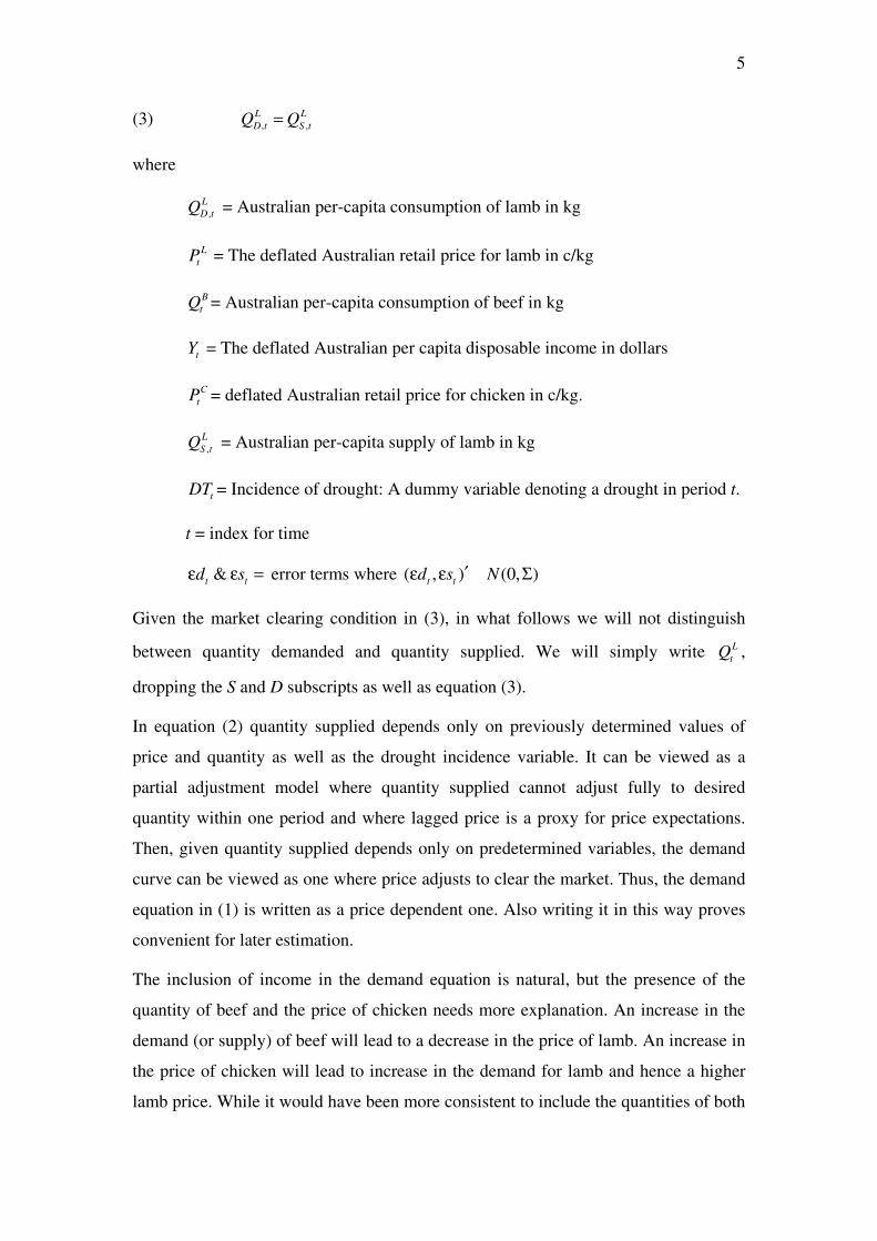
Draws of the parameters were used to obtain draws from the posterior densities for the

welfare changes using the procedure describe in Section 4. This information may be

18

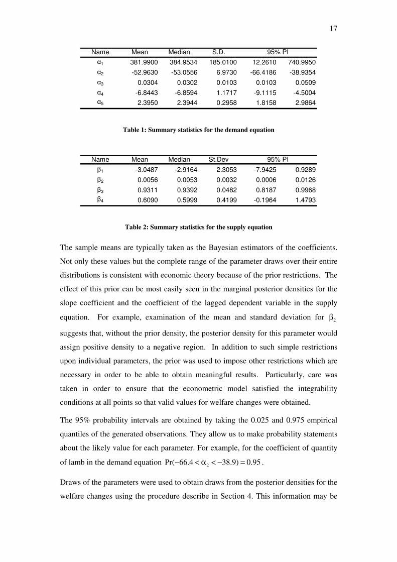
presented using tables of summary statistics or graphically using histograms as

estimates of the posterior densities. The summary statistics are presented in Table 3.

Estimates of the posterior densities are presented diagrammatically in Figures 2, 3 and

4.

Name Mean Median S.D

∆CS D 18.1920 18.7201 5.9317 14.8874 22.2448

∆CS S 18.1990 18.6071 6.4600 14.4044 22.5119

∆PS D 5.1668 4.1288 4.2562 2.0706 7.0271

∆PS S 5.1715 4.0710 4.4299 2.0243 6.9740

∆TS D 23.3590 23.6778 5.0170 20.5143 26.5871

∆TS S 23.3710 23.5811 6.0572 19.8347 27.2275

95% PI

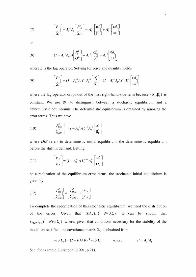
Table 1 Summary Statistics for Posterior Densities of Welfare Changes

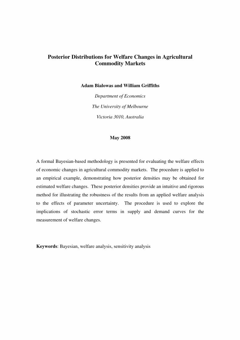
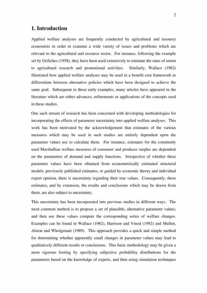
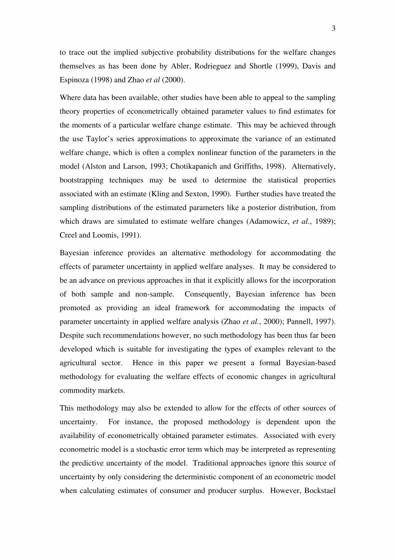
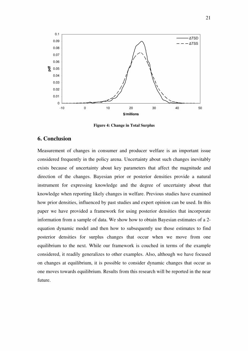
The posterior distributions for the deterministic welfare changes indicate a domestic

1% increase in the demand for lamb will results in an unambiguous increase in social

welfare. The magnitude of the increase is given by the posterior density for the

change in deterministic total surplus, D D D

TS CS PS∆ = ∆ + ∆ . From this density we

see that the magnitude of the gain is expected to lie between $20.5 million to $26.6

million with a point estimate given by the mean of $23.3 million. The distribution of

this welfare gain amongst consumer and producer groups indicates that consumers are

the primary beneficiaries, appropriating the majority of the gain. The posterior

density for the deterministic change in consumer surplus, D

CS∆ , indicates that

consumers’ welfare increases by between $14.9 million and $22.2 million and has a

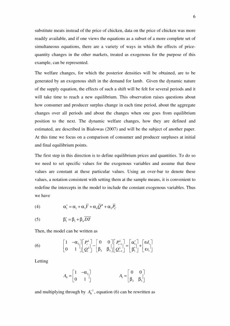
mean of $18.2 million. Producers are able to appropriate only a relatively small

proportion of the benefits from the demand shift. The posterior density for the

deterministic change in producer surplus, D

PS∆ , indicates that the total benefit

accruing to producers lies between $2.1 million and $7 million and has a mean of $5.2

million.

The posterior densities pertaining to the stochastic versions of the alternative welfare

measures produce results which are almost identical to those for the deterministic

specifications. It can be seen from Table 3 that summary statistics used to describe

the posterior densities for both the deterministic and stochastic welfare measures

differ only in the third or later digit. What this result implies is that, in this particular

example, the measurement of consumer and producer surplus changes are not

19

sensitive to the way in which the error terms have been introduced. Although the

difference is small, the stochastic changes do have higher standard deviations,

reflecting the additional uncertainty that arises from the error terms and the additional

uncertainty from estimation of the error covariance matrix. This additional uncertainty

can also be seen from the comparison of the posterior densities for the deterministic

and stochastic changes that appears in the figures. Those for the stochastic changes

have a slightly greater spread.

0

0.01

0.02

0.03

0.04

0.05

0.06

0.07

0.08

0.09

-10 0 10 20 30 40 50

$/millions

pd

f

∆CSD

∆CSS

Figure 2: Change in Consumer Surplus

There is another observation that can be made from the figures. Economic theory

implies that both consumers and producer should gain from the demand shift. Once

the new equilibrium has been reached consumers gain because they are able to

consumer more lamb at a lower price. Similarly, once the demand shift has occurred

producers gain because they are able to sell more lamb at a higher price. These results

imply the histograms should assign zero weight to negative regions of the welfare

changes. The histograms describing the deterministic welfare changes can be seen to

conform to this expectation as they are all truncated at zero. This is most obviously

the case for the posterior density for D

PS∆ , although it is also present in the posteriors

for the other welfare measures. It is most noticeable for D

PS∆ because the truncation

occurs in a region of high density as opposed to the tails. In contrast, the posterior

densities for the stochastic welfare changes all assign a small amount of weight to

20

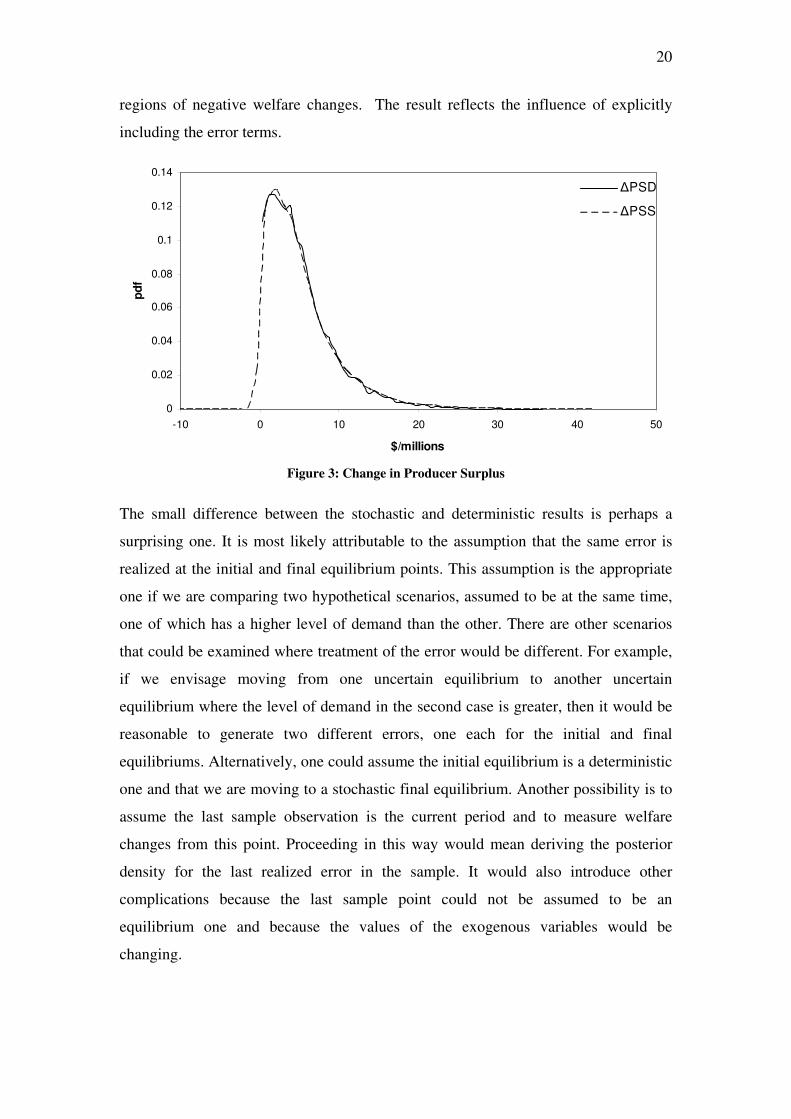
regions of negative welfare changes. The result reflects the influence of explicitly

including the error terms.

0

0.02

0.04

0.06

0.08

0.1

0.12

0.14

-10 0 10 20 30 40 50

$/millions

pd

f

∆PSD

∆PSS

Figure 3: Change in Producer Surplus

The small difference between the stochastic and deterministic results is perhaps a

surprising one. It is most likely attributable to the assumption that the same error is

realized at the initial and final equilibrium points. This assumption is the appropriate

one if we are comparing two hypothetical scenarios, assumed to be at the same time,

one of which has a higher level of demand than the other. There are other scenarios

that could be examined where treatment of the error would be different. For example,

if we envisage moving from one uncertain equilibrium to another uncertain

equilibrium where the level of demand in the second case is greater, then it would be

reasonable to generate two different errors, one each for the initial and final

equilibriums. Alternatively, one could assume the initial equilibrium is a deterministic

one and that we are moving to a stochastic final equilibrium. Another possibility is to

assume the last sample observation is the current period and to measure welfare

changes from this point. Proceeding in this way would mean deriving the posterior

density for the last realized error in the sample. It would also introduce other

complications because the last sample point could not be assumed to be an

equilibrium one and because the values of the exogenous variables would be

changing.

21

0

0.01

0.02

0.03

0.04

0.05

0.06

0.07

0.08

0.09

0.1

-10 0 10 20 30 40 50

$/millions

pd

f

∆TSD

∆TSS

Figure 4: Change in Total Surplus

6. Conclusion

Measurement of changes in consumer and producer welfare is an important issue

considered frequently in the policy arena. Uncertainty about such changes inevitably

exists because of uncertainty about key parameters that affect the magnitude and

direction of the changes. Bayesian prior or posterior densities provide a natural

instrument for expressing knowledge and the degree of uncertainty about that

knowledge when reporting likely changes in welfare. Previous studies have examined

how prior densities, influenced by past studies and expert opinion can be used. In this

paper we have provided a framework for using posterior densities that incorporate

information from a sample of data. We show how to obtain Bayesian estimates of a 2-

equation dynamic model and then how to subsequently use those estimates to find

posterior densities for surplus changes that occur when we move from one

equilibrium to the next. While our framework is couched in terms of the example

considered, it readily generalizes to other examples. Also, although we have focused

on changes at equilibrium, it is possible to consider dynamic changes that occur as

one moves towards equilibrium. Results from this research will be reported in the near

future.

22

References

Abler, D. G., A. G. Rodriguez, and J. Shortle (1999). "Parameter Uncertainty in CGE

Modeling of the Environmental Impacts of Economic Policies."

Environmental and Resource Economics 14: 75-94.

Adamowicz, W. L., J. J. Fletcher and T. Graham-Tomasi (1989). "Functional Form

and the Statistical Properties of Welfare Measures." American Journal of

Agricultural Economics 71(May): 414-221.

Alston, J. M. and D. M. Larson (1993). "Hicksian vs. Marshallian Welfare Measures:

Why Do We Do What We Do?" American Journal of Agricultural Economics

75(August): 764-769.

Bialowas, A. (2007), “Using Bayesian Inference to Accommodate Parameter

Uncertainty in the Estimation of Welfare Markets in Agricultural Commodity

Markets” forthcoming PhD Dissertation, University of Melbourne.

Bockstael, N. E. and I. E. Strand (1987). "The Effect of Common Sources of

Regression Error on Benefit Estimates." Land Economics 63(1): 11-20.

Chao, J. C. and P. C. B. Phillips (1998). "Posterior Distributions in Limited

Information Analysis Of The Simultaneous Equations Model Using The

Jeffreys Prior." Journal of Econometrics 87: 49-86.

Chotikapanich, D. and W. E. Griffiths (1998). "Canarvon Gorge: A Comment on the

Sensitivity Analysis of Consumer Surplus Estimation." Australian Journal of

Agricultural and Resource Economics 42(3): 249-261.

Creel, M. D. and J. B. Loomis (1991). "Confidence Intervals for Welfare Measures

with Application to a Problem of Truncated Counts." The Review of

Economic Studies 73(2): 370-370.

Davis, G. C. and M. C. Espinoza (1998). "A Unified Approach to Sensitivity Analysis

in Equilibrium Displacement Models." American Journal of Agricultural

Economics 80: 868-879.

Griliches, Z. (1958). "Research Costs and Social Returns: Hybrid Corn and Related

Innovations." The Journal of the Political Economy 66(5): 419-431.

Harrison, G. W. and H. D. Vinod (1992). "The Sensitivity Analysis of Applied

General Equilibrium Demand Models: Completely Randomized Factorial

Sampling Designs." The Review of Economics and Statistics 74: 357-362.

23

Kleibergen, F. and H. K. van Dijk (1994). "On The Shape Of The

Likelihood/Posterior In Cointegration Models." Econometric Theory 10: 514-

551.

Kling, C. L. (1992). "Some Results on the Variance of Welfare Estimates from

Recreational Demand Models." Land Economics 68(3): 318-28.

Kling, C. L. and R. J. Sexton (1990). "Bootstrapping in applied welfare analysis."

American Journal of Agricultural Economics 72(2): 406-418.

Lütkepohl, H. (1991). Introduction to Multiple Time Series Analysis. Berlin, Springe-

Verlag.

Mullen, J. D., J. M. Alston and M. K. Wohlgenant. (1989). "The impact of farm and

processing research on the Australian wool industry." Australian Journal of

Agricultural and Resource Economics 33(1): 32-47.

Pannell, D. J. (1997). "Sensitivity Analysis of Normative Econometric Models:

Theoretical Framework and Practical Strategies." Agricultural Economics 16:

139-152.

Vere, D., G. R. Griffith and R. Jones (2000). The Specification, Estimation and

Validation of a Quarterly Structural Econometric Model of the Australian

Grazing Industries. Adelaide, CRC for Weed Management Systems: 56.

Wallace, T. D. (1962). "Measures of social costs of agricultural programs." Journal of

Farm Economics 44(2): 580-97.

Zhao, X., W. E. Griffiths, G. R. Griffith and J. D. Mullen (2000). "Probability

Distributions for Economic Surplus Changes: The Case of Technical Change

in the Australian Wool Industry." The Australian Journal of Agricultural and

Resource Economics 44(1): 83-106.