Post-processing of solutions of incompressible Navier

ANZIAM J. 50 (CTAC2008) pp.C90–C106, 2008 C90

Post-processing of solutions of incompressibleNavier–Stokes equations on rotating spheres

M. Ganesh1 Q. T. Le Gia2

(Received 14 August 2008; revised 03 October 2008)

Abstract

We describe a post-processing technique (requiring only solutionsof linear stationary problems) to improve the resolution of Galerkin so-lutions of the time dependent nonlinear incompressible Navier–Stokesequations on the rotating unit sphere. Numerical experiments illus-trate the advantage of this more efficient method to simulate highermodes to approximate the divergence-free velocity field.

Contents

1 Introduction C91

2 The NSE on the rotating surface C93

http://anziamj.austms.org.au/ojs/index.php/ANZIAMJ/article/view/1436gives this article, c© Austral. Mathematical Soc. 2008. Published October 18, 2008. issn1446-8735. (Print two pages per sheet of paper.)

http://anziamj.austms.org.au/ojs/index.php/ANZIAMJ/article/view/1436

1 Introduction C91

3 A post-processing pseudospectral method C95

4 Numerical results C98

References C105

1 Introduction

The pseudospectral Galerkin method is a standard approach for computermodelling of the large scale atmospheric dynamics through the Navier–Stokesequations (nse) on the rotating Earth, see for example the recent work byFengler and Freeden [3] and references therein. The computable pseudospec-tral solution with N modes, approximating the unknown tangential surfacedivergence free velocity field of the nse, is of the form

uN =

N∑n=1

∑|m|≤n

αn,m(t)Zn,m, (1)

where Zn,m are the tangential surface divergence free eigenfunctions of theStokes operator on the chosen manifold, approximating the shape of theEarth. The rotating manifold was chosen to be the unit sphere by Fengler andFreeden [3]. (A standard surface model to study the atmospheric circulationon large planets is the sphere.) The number of time dependent unknownsin (1) is N2 + 2N and in pseudospectral methods these are obtained by firstprojecting the spatial part of the nse into the approximation space spannedby the N2 + 2N eigenfunctions, leading to the Galerkin (Fourier coefficient)equations, and then simulating the resulting (N2+2N)-dimensional nonlinearstiff ordinary differential systems in time. At each small time step of theevolution process the computational cost is dominated by setting up of thequadratic nonlinearity in the projected nse with O(N4) terms. Recall thateach Fourier coefficient requires integration on the sphere and approximationby quadratures which substantially increases the computational complexity.

1 Introduction C92

In order to obtain a fine resolution in the approximate velocity field, thevalue of N in (1) needs to be high. In the case of three dimensional time-dependent nonlinear partial differential equations, due to O(N4) complexityin setting up the nonlinear equations at each time step and evolving over along period of time, it is desirable to simulate with as small a value of N aspossible and yet obtain accurate velocity and pressure fields.

In particular, for the nse on periodic domains, after solving appropriatenonlinear time dependent systems only for low frequency approximations,one may obtain some of the remaining modes using approximate inertialmanifolds (Marion and Temam [8]). The exact inertial manifold is an opera-tor that determines the high frequency modes as a function of the computedlow frequency modes.

There are several ways to approximate the exact inertial manifold. Forexample one may restrict to 2N modes and then, based on the physicalbehaviour of the velocity field, use a linearised version of the nse. One suchwell known approximate inertial manifold method, leading to higher modes inthe velocity field from low frequency modes, is called the nonlinear Galerkinmethod, introduced by Marion and Temam [8] for the nse on bounded twodimensional domains with the nonslip boundary condition or on the plane R2

with periodic boundary conditions. For the rotating sphere model, Fenglerand Freeden [3] used the nonlinear Galerkin method to obtain approximatevelocity fields with 2N modes.

The nonlinear Galerkin method has the advantage of reducing the non-linearity in the evolution system of the standard Galerkin approximations.However, for each small positive evolution time step, to obtain the low fre-quency nonlinear Galerkin solutions, the corresponding high frequency modesshould be computed as well. In particular, the main disadvantage of the non-linear Galerkin method [3] is that for computing the 2N modes, a 4(N2 +N)-dimensional coupled system of differential equations needs to be simulated,with the first (N2 + 2N)-dimensional equation being nonlinear and the restbeing linear elliptic problems.


An ideal approach would be to first compute low frequency approxima-tions, say uN(t), for all t ∈ [0, T ] and then, for any particular desired time t∗,obtain high-resolution modes by solving just one simple stationary equationusing uN(t∗). Such a method, known as the post-processing technique, wasintroduced by Archilla et al. [1] as a novel approach to approximate inertialmanifolds. This method was applied for some parabolic problems on do-mains and yielded solutions with accuracy similar to the nonlinear Galerkinsolutions.

This article develops a post-processing version of the recent work [5]on the pseudospectral quadrature Galerkin method for the nse on rotat-ing spheres. We recall the weak form of the nse in the next section anddescribe the post-processing approach in Section 3. Numerical experimentsin Section 4 for a known velocity field with 2N Fourier modes and a bench-mark velocity flow generated by a random initial velocity field with Reynoldsnumber of the order 104 highlight the efficiency of this post-processing ap-proach.

2 The NSE on the rotating surface

We are interested in simulating a tangential velocity flow on the unit sphere S,denoted by u = u(x, t) = (u1(x, t), u2(x, t), u3(x, t))

T , x ∈ S and t ∈ [0, T ],with pressure p = p(x, t), satisfying the the incompressible nse [3, 6, 7, 9]

∂

∂tu +∇uu − ν∆u + ω× u +

1

ρGradp = f on S , (2)

u|t=0 = u0 , Div u = 0 on S, (3)

where the velocity flow is driven by the external field f = f(x, t), the rotationeffect is included in the normal vector field Coriolis term ω(x) = 2xΩ cos θ ,with constant rotation rate Ω, cos θ being the vertical third component of


x ∈ S and θ is the latitudinal variable. In (2), ν and ρ are respectively theconstant viscosity and density of the fluid.

Note that all spatial differential operators in (2)–(3) are defined on thesurface S. Among these, the surface divergence and gradient, denoted respec-tively by Div,Grad, are well known [6, 7], and the vector Laplace–Beltramioperator -∆ satisfies

− ∆v = Curl Curlx v − Grad Div v (4)

where the rate of rotation of a scalar function v, a normal vector field w =

wx , and a tangential vector field v on S are respectively defined by

Curl v = −x×Grad v , Curl w = −x×Gradw , Curlx v = −x Div(x×v).

In (2), the nonlinear term ∇uu is the covariant derivative

2∇wv = − Curl(w × v) + Grad(w · v) − v Div w + w Div v

− v × Curlx w − w × Curlx v . (5)

Restriction of the vector Laplace–Beltrami operator in (4) to the tangentialdivergence free functions reduces to the Stokes operator

A = Curl Curlx = −∆PCurl, (6)

where PCurl is the projection onto the space of smooth tangential divergencefree functions, denoted throughout by V . The infinite dimensional space Vis spanned by all polynomial eigenfunctions of the Stokes operator of degreen = 1, 2, . . . . For a fixed degree n, there are 2n + 1 degree n orthonormaleigenfunctions, denoted throughout by Zn,m, m = −n, . . . , n . Here theorthonormality is with respect to the L2-inner product (·, ·) for vector fields(and the associated L2-norm is denoted throughout by ‖ · ‖).

The next step is to remove the pressure term Gradp in (2). This isachieved by a weak formulation. That is, multiply (2) by functions in V andintegrate using the Gauss surface divergence theorem to remove Gradp:

(Gradp,w) :=

∫S

Gradp · w dS = −

∫S

p ·Div w dS = 0 , w ∈ V. (7)


For the nonlinear term in the weak formulation of (2), we consider

b(v,w, z) = (∇vw, z) =

∫S

∇vw · zdS , v,w, z ∈ V . (8)

The Coriolis operator on V is defined by

(Cv)(x) = ω(x)× v(x) = ω(x)(x× v), ω(x) = 2Ω cos θ ,

for v ∈ V and x ∈ S . Thus, a weak form of the nse (2)–(3) is

∂

∂t(u,v)+b(u,u,v)+ν(Curlx u,Curlx v)+(Cu,v) = (f ,v), v ∈ V , (9)

or in operator form with (B(u,u),v) = b(u,u,v), (9) is written as

∂

∂tu + νAu + B(u,u) + Cu = f , u(0) = u0 . (10)

3 A post-processing pseudospectral method

The pseudospectral quadrature Galerkin method for the nse was developedand analysed in detail by Ganesh et al. [5] with approximate velocity in

VN := spanZn,m : n = 1, . . . ,N , m = −n, . . . , n. (11)

Let ΠN be the orthogonal projection from V onto VN and let QN = I−ΠN .The solution of (9) is decomposed uniquely as

u = pN + qN , pN = ΠNu , qN = QNu .

Details described by Ganesh et al. [5] lead to computation and analysis of

uN(t) :=

N∑n=1

∑|m|≤n

αn,m(t)Zn,m , (12)


duN

dt+ ΠNB(uN,uN) + νAuN + CuN = ΠNf , uN(0) = ΠNu0 ,(13)

where we used that A and C map VN to VN because Zn,m are eigenfunctionsof A, for n = 1, . . . ,N , m = −n, . . . , n , and (CZn,m,Zj,k) = 0 if n 6= j orm 6= k , for j = 1, 2, . . . and k = −j, . . . , j .

The system (13) has N2 + 2N coupled ordinary differential equationsfor the unknown coefficients αn,m(t) in (12). Error analysis by Ganesh etal. [5] gives a spectrally accurate upper bound for ‖u − uN‖. For a lowerbound, note that the Galerkin error u − uN can never be smaller than thebest-approximation error u − pN = qN , that is

‖u − uN‖ ≥ ‖u − pN‖ = ‖qN‖.

To construct a solution with higher resolution, we rewrite (10) as

dpN

dt+ (νA + C)pN + ΠNB(pN + qN,pN + qN) = ΠNf , pN ∈ VN , (14)

dqN

dt+ (νA + C)qN +QNB(pN + qN,pN + qN) = QNf , qN ∈ V \ VN .

(15)

The existence of a function Φ such that qN = Φ(pN) was proven by severalresearchers (Temam and Wang [9] for example). The graph of Φ is known asthe inertial manifold. The existence of the inertial form suggests that in thefirst equation (14), qN may be replaced by Φ(pN) to obtain solutions withhigh resolution, but an analytical or computable form of the exact inertialmanifold is not known in general.

The next step is to consider a computable Φapp that approximates theexact inertial form Φ. The graph of Φapp, (v, Φapp(v)) | v ∈ VN is knownas an approximate inertial manifold. A concrete representation of Φapp canbe obtained using the observation by Foias et al. [4], that, under certainconstraints, in (15), terms containing qN other than (νA + C)qN can be


considered negligible compared to other terms in the full system. Hencefrom (15), the observation leads to an approximation

Φapp(pN) = Φ1(pN) := (νA + C)−1QN[f − B(pN,pN)]. (16)

Approximating QN by QN = Π2N−ΠN yields the computable approximation

Φapp(pN) = Φ1(pN) := (νA + C)−1QN[f − B(pN,pN)]. (17)

The nonlinear Galerkin method is based on (17). More precisely, to obtainnonlinear Galerkin solutions with 2N modes, we get a 4(N2+N)-dimensionalcoupled system, with the first N2 + 2N equations given by (14) with qN

replaced by Φ1(pN) and the remaining 3N2 + 2N equations for the un-known Φ1(pN) given by (17), leading to the system requiring higher res-olution solutions for simulation to move from one time step to the next.Thus each time step requires solutions of elliptic problems on the surface.

A less expensive approach is the post-processing Galerkin method, whichwas proposed initially for partial differential equations on periodic domainsby Archilla et al. [1]. The post-processing algorithm to compute a field wN

with 2N modes, approximating the velocity field u of (2)–(3) at any fixedtime t∗ is to

1. use a pseudospectral quadrature Galerkin algorithm to compute uN(t∗)

in (12)–(13);

2. solve the linear stationary elliptic problem

(νA + C)zN = Q2N

f − B

(uN(t∗),uN(t∗)

), Q2N = Π2N − ΠN ;

3. The new post-processed higher resolution approximation to the velocityfield u(t∗) is wN(t∗) := uN(t∗) + zN .

In the above post-processing algorithm, 2N can be replaced by cN, for anyinteger c ≥ 2 . A complete mathematical analysis of the algorithm, following


details as described by Archilla et al. [1] and the recent work by Ganesh etal. [5], proving the spectral accuracy of the post-processed solution, is beyondthe scope of this article.

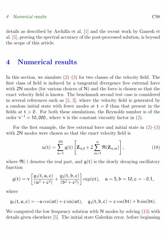
4 Numerical results

In this section, we simulate (2)–(3) for two classes of the velocity field. Thefirst class of field is induced by a tangential divergence free external forcewith 2N modes (for various choices of N) and the force is chosen so that theexact velocity field is known. The benchmark second test case is consideredin several references such as [2, 3], where the velocity field is generated bya random initial state with fewer modes at t = 0 than that present in thefields at t > 0 . For both these simulations, the Reynolds number is of theorder ν−1 = 10, 000 , where ν is the constant viscosity factor in (2).

For the first example, the free external force and initial state in (2)–(3)with 2N modes were chosen so that the exact velocity field is

u(t) =

2N∑n=1

g(t)

[Zn,0 + 2

n∑m=1

<(Zn,m)

], (18)

where <(·) denotes the real part, and g(t) is the slowly decaying oscillatoryfunction

g(t) = ν

[g1(t, a, c)

(a2 + c2)+g2(t, b, c)

(b2 + c2)

]exp(ct), a = 5, b = 10, c = −0.1,

where

g1(t, a, c) = −a cos(at) + c sin(at), g2(t, b, c) = c cos(bt) + b sin(bt).

We computed the low frequency solution with N modes by solving (13) withdetails given elsewhere [5]. The initial state Galerkin error, before beginning


0 5 10 15 20 25 30 3510

−5

10−4

10−3

time

l 2 err

or

Error in post−processed solution with Galerkin initial state error = 1.243e−03

Error in post−processed solution with 2N = 100 modes

Figure 1: Error in post-processed solution with 2N = 100 and Galerkininitial state error 0.1243× 10−2.


the adaptive time simulation of (13), is measured by the l2-norm of theunused vector with Fourier coefficients of the modes N + 1 to 2N. Theadaptive time simulation error tolerance was chosen to be smaller than theinitial state Galerkin error. The power of the post-processing approach toapproximate the velocity field (18) is demonstrated in Figure 1, where thepost-processed solution error for all time is better than the initial Galerkinerror with N = 50 . (We observed similar results for various values of N.)

The second example is (2)–(3) with a random field initial state having20 modes and the external force being a tangential surface divergence free

field with only one non-vanishing time-dependent Fourier coefficient f(t)3,0 .These two source fields, given in Figure 2, are similar to those considered bymany researchers [2, 3, 5] and differ mainly by the randomness of the initialstate.

For this unknown velocity field test case, as discussed by Debussche etal. [2] and by Ganesh et al. [5], after a sufficient large time, the nth mode en-ergy spectrum decays with O(n−4) for n within the inertial range and decaysexponentially for n in the dissipation range. Hence in this random initial fieldtest case, the post-processing solution effect is seen mainly at earlier evolu-tion time periods. In particular, the evolution process is such that the initialrandom flow with several smaller structures will slowly evolve into regularflow with larger structures. Simulation of this flow was carried out first withN = 50 and then post-processed to obtain approximate velocity field with2N modes. The simulation results in Figure 3–5, for t = 10, 20, 30 high-light the power of the post-processing that captures the transition of initialrandom flow to a regular flow, while the standard Galerkin pseudospectralsolution with N = 50 leads to regular flow even at t = 10 .

Acknowledgments The support of the Australian Research Council underits Discovery and Centre of Excellence grant is gratefully acknowledged. Wethank the referees for their valuable comments on the article.


(a)

(b)

0 5 10 15 20 25 30 35−0.4

−0.2

0

0.2

0.4

0.6

0.8

1

time

Fou

rier

coef

ficie

nt f 3,

0(t)

f3,0

(t), the only non−zero Fourier coeffcient of f

Figure 2: (a) Random initial state u0; and (b) time dependent external

force Fourier coefficient f(t)3,0.


Figure 3: Velocity u50(t) (above) and post-processed velocity (below) att = 10 .





References C105

References

[1] B. G. Archilla, J. Novo, and E. S. Titi. Postprocessing the Galerkinmethod: a novel approach to approximate inertial manifolds. SIAM J.Numer. Anal., 35:941–972, 1998. doi:10.1137/S0036142995296096 C93,C97, C98

[2] A. Debussche, T. Dubois, and R. Temam. The nonlinear Galerkinmethod: a multiscale method applied to the simulation of homogeneousturbulent flows. Theoret. Comput. Fluid Dynamics, 7:279–315, 1995.doi:10.1007/BF00312446 C98, C100

[3] M. J. Fengler and W. Freeden. A nonlinear Galerkin scheme involvingvector and tensor spherical harmonics for solving the incompressibleNavier–Stokes equation on the sphere. SIAM J. Sci. Comput.,27:967–994, 2004. doi:10.1137/040612567 C91, C92, C93, C98, C100

[4] C. Foias, O. Manley, and R. Temam. Modelling of the interaction ofsmall and large eddies in two dimensional turbulence flows, RAIROModel. Math. Anal. Numer., 22:93–118, 1988. C96

[5] M. Ganesh, Q. T. Le Gia, and I. H. Sloan. A pseudospectral quadraturemethod for Navier–Stokes equations on rotating spheres. Preprint.http://www.mines.edu/~mganesh/NSE-08-pap.pdf C93, C95, C96,C98, C100

[6] A. A. Il’in. The Navier-Stokes and Euler equations on two dimensionalclosed manifolds, Math. USSR Sbornik, 69:559–579, 1991.doi:10.1070/SM1991v069n02ABEH002116 C93, C94

[7] A. A. Il’in and A. N. Filatov. On unique solvability of the Navier–Stokesequations on the two dimensional sphere. Soviet Math. Dokl., 38:9–13,1989. C93, C94

http://dx.doi.org/10.1137/S0036142995296096

http://dx.doi.org/10.1007/BF00312446

http://dx.doi.org/10.1137/040612567

http://www.mines.edu/~mganesh/NSE-08-pap.pdf

http://dx.doi.org/10.1070/SM1991v069n02ABEH002116

References C106

[8] M. Marion and R. Temam. Nonlinear Galerkin methods, SIAM J.Numer. Anal., 26:1139–1157, 1989. doi:10.1137/0726063 C92

[9] R. Temam and S. Wang, Inertial forms of Navier–Stokes equations onthe sphere. J. Funct. Anal., 117:215–24, 1993.doi:10.1006/jfan.1993.1126 C93, C96

Author addresses

1. M. Ganesh, Department of Mathematical and Computer Sciences,Colorado School of Mines, Golden, CO 80401, USA.mailto:[email protected]

2. Q. T. Le Gia, School of Mathematics and Statistics, University ofNew South Wales, Sydney, NSW 2052, Australia.mailto:mailto:[email protected]

http://dx.doi.org/10.1137/0726063

http://dx.doi.org/10.1006/jfan.1993.1126

mailto:[email protected]

mailto:mailto:[email protected]

Documents

Post-processing of solutions of incompressible Navier