Embed Size (px)
Citation preview

ETSI TS 102 250-6 V1.2.1 (2004-10)
Technical Specification
Speech Processing, Transmission and Quality Aspects (STQ);QoS aspects for popular services in GSM and 3G networks;
Part 6: Post processing and statistical methods
ETSI
ETSI TS 102 250-6 V1.2.1 (2004-10) 2
Reference RTS/STQ-00061m
Keywords 3G, GSM, network, QoS, service, speech
ETSI
650 Route des Lucioles F-06921 Sophia Antipolis Cedex - FRANCE
Tel.: +33 4 92 94 42 00 Fax: +33 4 93 65 47 16
Siret N° 348 623 562 00017 - NAF 742 C
Association à but non lucratif enregistrée à la Sous-Préfecture de Grasse (06) N° 7803/88
Important notice
Individual copies of the present document can be downloaded from: http://www.etsi.org
The present document may be made available in more than one electronic version or in print. In any case of existing or perceived difference in contents between such versions, the reference version is the Portable Document Format (PDF).
In case of dispute, the reference shall be the printing on ETSI printers of the PDF version kept on a specific network drive within ETSI Secretariat.
Users of the present document should be aware that the document may be subject to revision or change of status. Information on the current status of this and other ETSI documents is available at
http://portal.etsi.org/tb/status/status.asp
If you find errors in the present document, please send your comment to one of the following services: http://portal.etsi.org/chaircor/ETSI_support.asp
Copyright Notification
No part may be reproduced except as authorized by written permission. The copyright and the foregoing restriction extend to reproduction in all media.
© European Telecommunications Standards Institute 2004.
All rights reserved.
DECTTM, PLUGTESTSTM and UMTSTM are Trade Marks of ETSI registered for the benefit of its Members. TIPHONTM and the TIPHON logo are Trade Marks currently being registered by ETSI for the benefit of its Members. 3GPPTM is a Trade Mark of ETSI registered for the benefit of its Members and of the 3GPP Organizational Partners.
ETSI
ETSI TS 102 250-6 V1.2.1 (2004-10) 3
Contents
Intellectual Property Rights ................................................................................................................................6
Foreword.............................................................................................................................................................6
Introduction ........................................................................................................................................................7
1 Scope ........................................................................................................................................................8
2 References ................................................................................................................................................8
3 Definitions, symbols and abbreviations ...................................................................................................8 3.1 Definitions..........................................................................................................................................................8 3.2 Symbols..............................................................................................................................................................9 3.3 Abbreviations .....................................................................................................................................................9
4 Important measurement data types in mobile communications ...............................................................9 4.1 Data with binary values ....................................................................................................................................10 4.2 Data out of time-interval measurements...........................................................................................................10 4.3 Measurement of data throughput......................................................................................................................10 4.4 Data concerning quality measures....................................................................................................................10
5 Distributions and moments.....................................................................................................................11 5.1 Introduction ......................................................................................................................................................11 5.2 Continuous and discrete distributions...............................................................................................................12 5.3 Definition of density function and distribution function ..................................................................................12 5.3.1 Probability Distribution Function (PDF) ....................................................................................................12 5.3.2 Cumulative Distribution Function (CDF) ...................................................................................................13 5.4 Moments and quantiles.....................................................................................................................................13 5.5 Estimation of moments and quantiles...............................................................................................................15 5.6 Important distributions .....................................................................................................................................16 5.6.1 Continuous distributions .............................................................................................................................16 5.6.1.1 Normal distribution ...............................................................................................................................16 5.6.1.1.1 Standard normal distribution ...........................................................................................................17 5.6.1.1.2 Central limit theorem.......................................................................................................................18 5.6.1.1.3 Transformation to normality............................................................................................................18 5.6.1.2 Log-Normal distribution .......................................................................................................................18 5.6.1.2.1 Use-case: transformations................................................................................................................19 5.6.1.3 Exponential distribution ........................................................................................................................19 5.6.1.4 Weibull distribution ..............................................................................................................................20 5.6.1.5 Pareto distribution .................................................................................................................................21 5.6.1.6 Extreme distribution (Fisher-Tippett distribution) ................................................................................22 5.6.2 Testing distributions ...................................................................................................................................22 5.6.2.1 Chi-Square distribution with n degrees of freedom ..............................................................................23 5.6.2.1.1 Further relations...............................................................................................................................24 5.6.2.1.2 Relation to empirical variance .........................................................................................................24 5.6.2.2 Student t-distribution.............................................................................................................................24 5.6.2.2.1 Relation to normal distribution........................................................................................................25 5.6.2.3 F distribution .........................................................................................................................................26 5.6.2.3.1 Quantiles..........................................................................................................................................27 5.6.2.3.2 Approximation of quantiles .............................................................................................................27 5.6.2.3.3 Relations to other distributions........................................................................................................28 5.6.3 Discrete distributions ..................................................................................................................................28 5.6.3.1 Bernoulli distribution ............................................................................................................................28 5.6.3.2 Binomial distribution ............................................................................................................................29 5.6.3.3 Geometric distribution ..........................................................................................................................30 5.6.3.4 Poisson distribution...............................................................................................................................31 5.6.4 Transitions between distributions and appropriate approximations............................................................32 5.6.4.1 From binomial to Poisson distribution ..................................................................................................32 5.6.4.2 From binomial to Normal distribution ..................................................................................................32 5.6.4.3 From Poisson to Normal distribution ....................................................................................................32
ETSI
ETSI TS 102 250-6 V1.2.1 (2004-10) 4
5.6.5 Truncated distributions ...............................................................................................................................33 5.6.6 Distribution selection and parameter estimation.........................................................................................33 5.6.6.1 Test procedures .....................................................................................................................................33 5.6.6.1.1 Chi-Square test ................................................................................................................................33 5.6.6.1.2 Kolmogorov-Smirnov test ...............................................................................................................33 5.6.6.1.3 Shapiro-Wilk test.............................................................................................................................33 5.6.6.2 Parameter estimation methods ..............................................................................................................34 5.7 Evaluation of measurement data ......................................................................................................................34 5.7.1 Statistical tests ............................................................................................................................................34 5.7.1.1 Formulation of statistical tests...............................................................................................................34 5.7.1.2 Classes of statistical tests ......................................................................................................................35 5.7.1.3 Tests for normal and binomial data.......................................................................................................35 5.7.1.3.1 One-sample tests for normal data ....................................................................................................35 5.7.1.3.2 Two-sample tests for normal data....................................................................................................36 5.7.1.3.3 Test for binomial data......................................................................................................................37 5.7.1.4 Distribution-free tests for location ........................................................................................................38 5.7.1.4.1 Sign tests..........................................................................................................................................38 5.7.1.4.2 Sign rank test ...................................................................................................................................38 5.7.1.4.3 Wilcoxon rank sum test ...................................................................................................................39 5.7.2 Confidence interval.....................................................................................................................................39 5.7.2.1 Binomial distribution ............................................................................................................................40 5.7.2.2 Normal (Gaussian) distribution.............................................................................................................41 5.7.3 Required sample size for certain confidence levels ....................................................................................42
6 Visualization techniques.........................................................................................................................43 6.1 Visualization of static data ...............................................................................................................................43 6.1.1 Histograms..................................................................................................................................................43 6.1.2 Barplots.......................................................................................................................................................43 6.1.3 QQ-Plots .....................................................................................................................................................44 6.1.4 Boxplots......................................................................................................................................................44 6.2 Visualization of dynamic data ..........................................................................................................................45 6.2.1 Line Diagrams ............................................................................................................................................45 6.2.2 Temporal changing Boxplots......................................................................................................................45 6.2.3 MMQ-Plots .................................................................................................................................................46
7 Time series modelling ............................................................................................................................46 7.1 Descriptive characterization .............................................................................................................................47 7.1.1 Empirical moments .....................................................................................................................................48 7.1.2 Decomposition of time series......................................................................................................................49 7.1.3 Determination of the trend component .......................................................................................................50 7.1.3.1 Trend function types .............................................................................................................................51 7.1.3.1.1 Linear trend function .......................................................................................................................51 7.1.3.1.2 Polynomial trend function ...............................................................................................................51 7.1.3.1.3 Non-linear trend models ..................................................................................................................52 7.1.3.2 Trend estimation ...................................................................................................................................52 7.1.3.3 Transformation of time series by filtering.............................................................................................53 7.1.3.3.1 Linear filters ....................................................................................................................................54 7.1.3.3.2 Exponential filters ...........................................................................................................................56 7.1.4 Seasonal component ...................................................................................................................................57
8 Data aggregation ....................................................................................................................................58 8.1 Basic data aggregation operators......................................................................................................................58 8.2 Data sources, structures and properties ............................................................................................................59 8.2.1 Raw data .....................................................................................................................................................59 8.2.1.1 Performance data...................................................................................................................................59 8.2.1.2 Event data..............................................................................................................................................59 8.2.2 Key Performance Indicators / Parameters...................................................................................................60 8.3 Aggregation hierarchies ...................................................................................................................................60 8.3.1 Temporal aggregation .................................................................................................................................60 8.3.2 Spatial aggregation .....................................................................................................................................61 8.4 Parameter estimation methods..........................................................................................................................61 8.4.1 Projection method .......................................................................................................................................61 8.4.2 Substitution method ....................................................................................................................................61
ETSI
ETSI TS 102 250-6 V1.2.1 (2004-10) 5
8.4.3 Application of estimation methods .............................................................................................................62 8.4.4 Attributes of aggregation operators ............................................................................................................62 8.5 Weighted aggregation.......................................................................................................................................63 8.5.1 Perceived QoS ............................................................................................................................................63 8.5.2 Weighted quantiles .....................................................................................................................................64 8.6 Additional data aggregation operators..............................................................................................................65 8.6.1 MAWD and BH..........................................................................................................................................65 8.6.2 AVGn..........................................................................................................................................................65
9 Assessment of performance indices .......................................................................................................65 9.1 Estimation of performance parameters based on active service probing systems ............................................65 9.2 Monitoring concepts.........................................................................................................................................65 9.2.1 Control charts..............................................................................................................................................66 9.2.1.1 Shewhart control charts.........................................................................................................................66 9.2.1.2 CUSUM and EWMA charts..................................................................................................................66 9.2.2 Other alarming rules ...................................................................................................................................66 9.3 Methods for evaluation of objectives ...............................................................................................................66 9.3.1 Desirability functions..................................................................................................................................67 9.3.2 Loss functions .............................................................................................................................................67
Annex A (informative): Examples of statistical calculations ..............................................................68
A.1 Confidence intervals for binomial distribution.......................................................................................68 A.1.1 Step by step computation .................................................................................................................................68 A.1.2 Computation using statistical software.............................................................................................................70 A.1.2.1 Computation in R........................................................................................................................................70 A.1.2.2 Computation in Excel .................................................................................................................................71
A.2 Transition from binomial to normal distribution....................................................................................71
A.3 Definitions of EG 201 769 .....................................................................................................................72
A.4 Calculation of confidence intervals ........................................................................................................73 A.4.1 Estimated rate 5 %............................................................................................................................................73 A.4.2 Estimated rate 50 %..........................................................................................................................................74 A.4.3 Estimated rate 95 %..........................................................................................................................................74 A.4.4 Lower limit of confidence intervals according to Pearson-Clopper formula....................................................75 A.4.5 Upper limit of confidence intervals according to Pearson-Clopper formula ....................................................76 A.4.6 Span of confidence intervals according to Pearson-Clopper formula ..............................................................78
A.5 Different sample sizes ............................................................................................................................80
A.6 Calculation methods...............................................................................................................................82 A.6.1 Calculation of quantiles....................................................................................................................................82
A.7 Reporting of results ................................................................................................................................84 A.7.1 Methods to use .................................................................................................................................................84 A.7.2 Number of significant decimals........................................................................................................................85 A.7.3 Rounding of end results....................................................................................................................................85
Annex B (informative): Bibliography...................................................................................................86
History ..............................................................................................................................................................87

ETSI
ETSI TS 102 250-6 V1.2.1 (2004-10) 6
Intellectual Property Rights IPRs essential or potentially essential to the present document may have been declared to ETSI. The information pertaining to these essential IPRs, if any, is publicly available for ETSI members and non-members, and can be found in ETSI SR 000 314: "Intellectual Property Rights (IPRs); Essential, or potentially Essential, IPRs notified to ETSI in respect of ETSI standards", which is available from the ETSI Secretariat. Latest updates are available on the ETSI Web server (http://webapp.etsi.org/IPR/home.asp).
Pursuant to the ETSI IPR Policy, no investigation, including IPR searches, has been carried out by ETSI. No guarantee can be given as to the existence of other IPRs not referenced in ETSI SR 000 314 (or the updates on the ETSI Web server) which are, or may be, or may become, essential to the present document.
Foreword This Technical Specification (TS) has been produced by ETSI Technical Committee Speech Processing, Transmission and Quality Aspects (STQ).
The present document is part 6 of a multi-part deliverable covering the QoS aspects for popular services in GSM and 3G networks, as identified below:
Part 1: "Identification of Quality of Service aspects";
Part 2: "Definition of Quality of Service parameters and their computation";
Part 3: "Typical procedures for Quality of Service measurement equipment";
Part 4: "Requirements for Quality of Service measurement equipment";
Part 5: "Definition of typical measurement profiles";
Part 6: "Post processing and statistical methods";
Part 7: "Sampling methodology".
Part 1 identifies QoS aspects for popular services in GSM and 3G networks. For each service chosen QoS indicators are listed. They are considered to be suitable for the quantitatively characterization of the dominant technical QoS aspects as experienced from the end-customer perspective.
Part 2 defines QoS parameters and their computation for popular services in GSM and 3G networks. The technical QoS indicators, listed in part 1, are the basis for the parameter set chosen. The parameter definition is split into two parts: the abstract definition and the generic description of the measurement method with the respective trigger points. Only measurement methods not dependent on any infrastructure provided are described in the present document. The harmonized definitions given in the present document are considered as the prerequisites for comparison of QoS measurements and measurement results.
Part 3 describes typical procedures used for QoS measurements over GSM, along with settings and parameters for such measurements.
Part 4 defines the minimum requirements of QoS measurement equipment for GSM and 3G networks in the way that the values and trigger-points needed to compute the QoS parameter as defined in part 2 can be measured following the procedures defined in part 3. Test-equipment fulfilling the specified minimum requirements, will allow to perform the proposed measurements in a reliable and reproducible way.
Part 5 specifies test profiles which are required to enable benchmarking of different GSM or 3G networks both within and outside national boundaries. It is necessary to have these profiles so that when a specific set of tests are carried out then customers are comparing "like for like" performance.

ETSI
ETSI TS 102 250-6 V1.2.1 (2004-10) 7
Part 6 describes procedures to be used for statistical calculations in the field of QoS measurement of GSM and 3G network using probing systems.
Part 7 describes the field measurement method procedures used for QoS measurements over GSM where the results are obtained applying inferential statistics.
Introduction All the defined quality of service parameters and their computations are based on field measurements. That indicates that the measurements were made from customers point of view (full end-to-end perspective, taking into account the needs of testing).
It is assumed that the end customer can handle his mobile and the services he wants to use (operability is not evaluated at this time). For the purpose of measurement it is assumed:
• that the service is available and not barred for any reason;
• routing is defined correctly without errors; and
• the target subscriber equipment is ready to answer the call.
Voice quality values measured should only be employed by calls ended successfully for statistical analysis.
However, measured values from calls ended unsuccessfully (e.g. dropped) should be available for additional evaluations and therefore, must be stored.
Further preconditions may apply when reasonable.

ETSI
ETSI TS 102 250-6 V1.2.1 (2004-10) 8
1 Scope The present document describes definitions and procedures to be used for statistical calculations which are related to Quality of Service (QoS) measurements done by serving probing systems in mobile communications networks, especially GSM and 3G networks. Network performance measurements and their related post-processing are only marginally covered in the present document.
2 References The following documents contain provisions which, through reference in this text, constitute provisions of the present document.
• References are either specific (identified by date of publication and/or edition number or version number) or non-specific.
• For a specific reference, subsequent revisions do not apply.
• For a non-specific reference, the latest version applies.
Referenced documents which are not found to be publicly available in the expected location might be found at http://docbox.etsi.org/Reference.
[1] ETSI EG 201 769: "Speech Processing, Transmission and Quality Aspects (STQ); QoS parameter definitions and measurements; Parameters for voice telephony service required under the ONP Voice Telephony Directive 98/10/EC".
3 Definitions, symbols and abbreviations
3.1 Definitions For the purposes of the present document, the following terms and definitions apply:
rate: measurement result which is related to the portion of time during which it has been executed
NOTE: The denominator's unit is related to time.
ratio: measurement result which represents a subgroup of all single measurements is related to the total number of executed single measurements
NOTE: Usually, nominator and denominator share the same unit, namely a counter for measurements (subgroup/all).
ETSI
ETSI TS 102 250-6 V1.2.1 (2004-10) 9
3.2 Symbols For the purposes of the present document, the following symbols apply:
E(x)=µ Expected value of random variable x Var(x)=σ2 Variance of random variable x σ Standard deviation of random variable x f(x) Probability Density Function (PDF) of random variable x F(x) Cumulative Distribution Function (CDF) of random variable x S, x∈ S Set of discrete values or interval of values the random variable x may take IR Set of real numbers s, s2 Empirical standard deviation / variance, analogous to σ and σ2 (theoretical) qα α-Quantile
uα α-Quantile of standard normal distribution
x(i), x(1), x(n) i-th ordered value, minimum and maximum of a given data set xi, i =1,...,n
3.3 Abbreviations For the purposes of the present document, the following abbreviations apply:
3G Third Generation ARMA Auto-Regressive Moving Average AVGn Averaging Operator (regarding n days) BH Busy Hour BSC Base Station Controller CDF Cumulative Distribution Function or Cumulative Density Function (used synonymously) CUSUM CUmulated SUM EWMA Exponentially Weighted Moving Average GSM Global System for Mobile communications KPI Key Performance Indicator LSL Lower Specification Level MAWD Monthly Average Working Day MMQ-Plot Median-Mean-Quantile Plot MMS Multimedia Messaging Service MOS Mean Opinion Score MSC Mobile Switching Centre NE Network Element PDF Probability Density Function QoS Quality of Service QQ-Plot Quantile-Quantile Plot SMS Short Message Service USL Upper Specification Level
4 Important measurement data types in mobile communications
Appropriate data analysis methods should depend on the type of the given data as well as on the scope of the analysis. Therefore before analysis methods are described, different data types are introduced and differences between them are pointed out.
Four general categories of measurement results are expected when QoS measurements are done in mobile communications.
ETSI
ETSI TS 102 250-6 V1.2.1 (2004-10) 10
4.1 Data with binary values Single measurements related to the topics:
• service accessibility, service availability;
• service retainability, service continuity;
• error ratios, error probabilities;
in general show a binary outcome, i.e. only two outcomes are possible. This means the result of a single trial leads to a result which is either valued positive or negative related to the considered objective. The result may be recorded as decision-results Yes / No or True / False or with numerical values 0 = successful and 1 = unsuccessful (i.e. errors occur) or vice versa. Aggregation of trials of both types allows to calculate the according ratios which means the number of positive / negative results is divided by the number of all trials. Usually, the units of nominator and denominator are the same, namely number of trials.
EXAMPLE: If established voice calls are considered to test the service retainability of a voice telephony system, every successfully completed call leads to the positive result "Call completed", every unsuccessfully ended call is noticed as "Dropped call" which represents the negative outcome. After 10 000 established calls, the ratio of dropped calls related to all established calls can be calculated. The result is the call drop probability.
4.2 Data out of time-interval measurements Measurements related to the time domain occur in the areas:
• duration of a session or call;
• service access delay;
• round trip time and end-to-end delay of a service;
• blocking times, downtimes of a system.
The outcome of such measurements is the time span between two time stamps marking the starting and end point of the time periods of interest. Results are related to the unit "second" or multiples or parts of it. Depending on the measurement tools and the precision needed, arbitrarily small measurement units may be realized.
EXAMPLE: Someone can define the end-to-end delivery time for the MMS service by a measurement which starts when the user at the A party pushes the "Send" button and which stops when the completely received MMS is signalled to the user at the B party.
4.3 Measurement of data throughput Measurements related to data throughput result in values which describe the ratio of transmitted data volume related to the required portion of time. The outcome of a single measurement is the quotient of both measures. Used units are "bit" or multiples thereof for the data amount and "second" or multiples or parts thereof for the portion of time.
EXAMPLE: If a data amount of 1 Mbit is transmitted within a period of 60 seconds, this results in a mean data rate of approximately 16,66 kbit/s.
4.4 Data concerning quality measures Examples are given by the quality of data transfer which may be measured by its speed or evaluations of speech quality measured on a scale, respectively.

ETSI
ETSI TS 102 250-6 V1.2.1 (2004-10) 11
Measurements related to audio-visual quality can be done objectively by algorithms or subjectively by human listeners. The outcome of audio-visual quality evaluation is related to a scaled value which is called Mean Opinion Score (MOS) for subjective testing. Thereby two types of quality measurement are distinguished subjective and objective measurements. If quantitative measures are identified which are highly correlated to the quality of interest, this will simplify the analysis. However, if this is not possible, some kind of evaluation on a standardized scale by qualified experts is needed. The result may therefore be given either as the measurement result or as a mark on a pre-defined scale.
EXAMPLE: Within a subjective test, people are asked to rate the overall quality of video samples which are presented to them. The allowed scale to rate the quality is defined in the range from 1 (very poor quality) to 5 (brilliant quality).
Table 4.1 summarizes the different kinds of QoS related measurements, typical outcomes and some examples.
Table 4.1: QoS related measurements, typical outcomes and examples
Category Relevant measurement types Examples Binary values Service accessibility, service availability
Service retainability, service continuity Error ratios, error probabilities
Service accessibility telephony, service non-availability SMS Call completion rate, call drop rate Call set-up error rate
Duration values Duration of a session or call Service access delay Round trip time, end-to-end delay Blocking times, system downtimes
Mean call duration Service access delay WAP ICMP Ping roundtrip time Blocking time telephony, SGSN downtime
Throughput values Throughput Mean data rate GPRS Peak data rate UMTS
Content quality values Audio-visual quality MOS scores out of subjective testing
5 Distributions and moments
5.1 Introduction The objective of data analyses is to draw conclusions about the state of a process based on a given data set, which may or may not be a sample of the population of interest. If distributions are assumed, these specify the shape of the data mass up to parameters associated with each family of distributions specifying properties like the mean of the data mass. Location or dispersion shifts of the process will in general result in different parameter estimates specifying the distribution. Therefore the information available from the data is compressed into one or few sufficient statistics specifying the underlying distribution.
Many statistical applications and computations rely in some sense on distributional assumptions, which are not always explicitly stated. Results of statistical measures are often only sensible if underlying assumptions are met and therefore only interpretable if users know about these assumptions.
This clause is organized as follows. Firstly, distributions, moments and quantiles are introduced in theory in clauses 5.2 to 5.4. This part of the document is based on the idea of random variables having certain distributions. Random variables do not take single values but describe the underlying probability model of a random process. They are commonly denoted by:
X ~ distribution (parameters)
From the distributional assumptions, moments and quantiles of random variables are derived in theory.
Data is often viewed as being realizations of random variables. Therefore, data analysis mainly consists of fitting an appropriate distribution to the data and drawing conclusions based on this assumption. Clause 5.5 briefly summarizes the estimation of moments and quantiles.
Subsequently, a number of important distributions is introduced in clause 5.6, each of which is visualized graphically to give an idea of meaningful applications. Within this clause, testing distributions are also introduced as they are needed in clause 5.7 for the derivation of statistical tests.
ETSI
ETSI TS 102 250-6 V1.2.1 (2004-10) 12
5.2 Continuous and discrete distributions The main difference between the data types described above can be explained in terms of continuous and discrete distributions. Data with binary values follow a discrete distribution, since the probability mass is distributed only over a fixed number of possible values. The same holds for quality measurements with evaluation results on a scale with a limited number of possible values (i.e. marks 1 to 6 or similar).
On the contrary, time-interval measurements as well as quality measurements based on appropriate quantitative variables may take an infinitely large number of possible values. In theory, since the number of possible outcomes equals infinity, the probability that a single value is exactly realized is zero. Probabilities greater than zero are only realized for intervals with positive width. In practice, each measurement tool will only allow a limited precision resulting in discrete measurements with a large number of possible outcomes. Nevertheless, data from measurement systems with reasonable precision are treated as being continuous.
Formal definitions for continuous and discrete distributions are based on probability density functions as will be described in the following.
5.3 Definition of density function and distribution function
5.3.1 Probability Distribution Function (PDF)
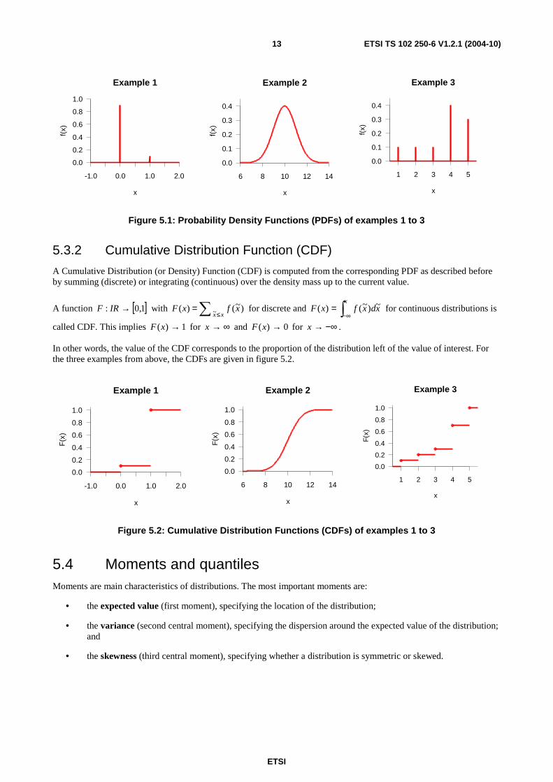
Probability Density Functions (PDF) specify the probability mass either for single outcomes (discrete distributions) or for intervals (continuous distributions).
A PDF is defined as a function [ )∞→ ,0: IRf with properties:
i) 0)( ≥xf for all x∈ S.
ii) ∫ =S
dxxf 1)( for continuous distributions or ∑ =S
xf 1)( for discrete distributions.
In other words, firstly the values of the PDF are always non-negative, meaning that negative probabilities are neither assigned to values nor intervals, and secondly the summation or integration over the PDF always results in 1 (= 100 %), meaning that any data value will always be realized.
EXAMPLE 1: A PDF for binary data may be given by
==
=0 x :9,0
1 x :1,0)(xf , which implies that the probability for
a faulty trial (x=1) is 10 %, while tests are completed successfully with probability 90 %.
EXAMPLE 2: For time-interval measurements PDFs may take any kind of shape, as an example a normal distribution with mean 10 (seconds) is assumed here. The PDF for this distribution is given by
( ){ }221
21 10exp)( −−= xxfπ
. Other examples for continuous distributions will follow later on.
EXAMPLE 3: If for instance categories for speech quality are defined as 1 = very poor up to 5 = brilliant, a PDF
for the resulting data may be given by
{ }
==
∈=
5:3,0
4:4,0
3,2,1:1,0
)(
x
x
x
xf .
Figure 5.1 summarizes all three assumed example PDFs for the different data types.
ETSI
ETSI TS 102 250-6 V1.2.1 (2004-10) 13
Example 1
x
f(x)
-1.0 0.0 1.0 2.0
0.0
0.2
0.4
0.6
0.8
1.0
Example 2
x
f(x)
6 8 10 12 14
0.0
0.1
0.2
0.3
0.4
Example 3
x
f(x)
1 2 3 4 5
0.0
0.1
0.2
0.3
0.4
Figure 5.1: Probability Density Functions (PDFs) of examples 1 to 3
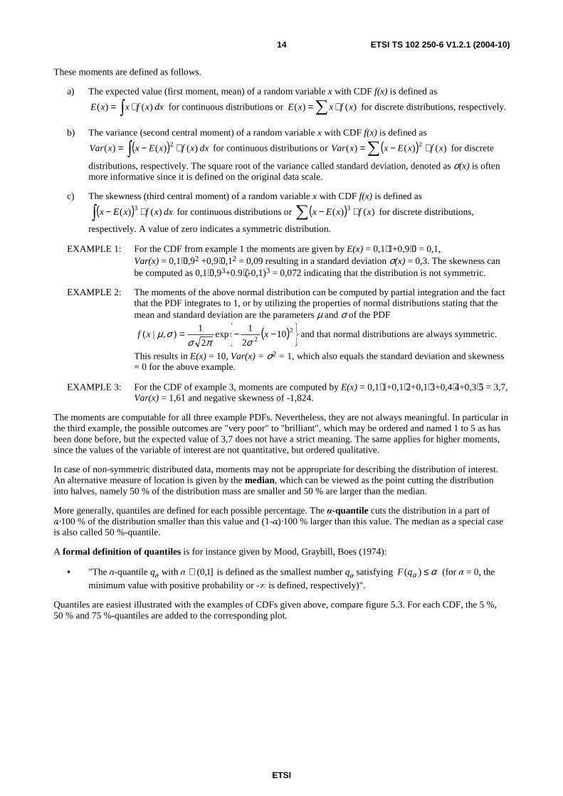
5.3.2 Cumulative Distribution Function (CDF)
A Cumulative Distribution (or Density) Function (CDF) is computed from the corresponding PDF as described before by summing (discrete) or integrating (continuous) over the density mass up to the current value.
A function [ ]1,0: →IRF with ∑ ≤=
xxxfxF ~
)~()( for discrete and ∫ ∞−=
xxdxfxF ~)~()( for continuous distributions is
called CDF. This implies 1)( →xF for ∞→x and 0)( →xF for −∞→x .
In other words, the value of the CDF corresponds to the proportion of the distribution left of the value of interest. For the three examples from above, the CDFs are given in figure 5.2.
Example 1
x
F(x
)
-1.0 0.0 1.0 2.0
0.0
0.2
0.4
0.6
0.8
1.0
Example 2
x
F(x
)
6 8 10 12 14
0.0
0.2
0.4
0.6
0.8
1.0
Example 3
x
F(x
)
1 2 3 4 5
0.0
0.2
0.4
0.6
0.8
1.0
Figure 5.2: Cumulative Distribution Functions (CDFs) of examples 1 to 3
5.4 Moments and quantiles Moments are main characteristics of distributions. The most important moments are:
• the expected value (first moment), specifying the location of the distribution;
• the variance (second central moment), specifying the dispersion around the expected value of the distribution; and
• the skewness (third central moment), specifying whether a distribution is symmetric or skewed.
ETSI
ETSI TS 102 250-6 V1.2.1 (2004-10) 14
These moments are defined as follows.
a) The expected value (first moment, mean) of a random variable x with CDF f(x) is defined as
∫ ⋅= dxxfxxE )()( for continuous distributions or ∑ ⋅= )()( xfxxE for discrete distributions, respectively.
b) The variance (second central moment) of a random variable x with CDF f(x) is defined as
( )∫ ⋅−= dxxfxExxVar )()()( 2 for continuous distributions or ( )∑ ⋅−= )()()( 2 xfxExxVar for discrete
distributions, respectively. The square root of the variance called standard deviation, denoted as σ(x) is often more informative since it is defined on the original data scale.
c) The skewness (third central moment) of a random variable x with CDF f(x) is defined as
( )∫ ⋅− dxxfxEx )()( 3 for continuous distributions or ( )∑ ⋅− )()( 3 xfxEx for discrete distributions,
respectively. A value of zero indicates a symmetric distribution.
EXAMPLE 1: For the CDF from example 1 the moments are given by E(x) = 0,1⋅1+0,9⋅0 = 0,1, Var(x) = 0,1⋅0,92 +0,9⋅0,12 = 0,09 resulting in a standard deviation σ(x) = 0,3. The skewness can be computed as 0,1⋅0,93+0.9⋅(-0,1)3 = 0,072 indicating that the distribution is not symmetric.
EXAMPLE 2: The moments of the above normal distribution can be computed by partial integration and the fact that the PDF integrates to 1, or by utilizing the properties of normal distributions stating that the mean and standard deviation are the parameters µ and σ of the PDF
( )
−−= 2
210
2
1exp
2
1),|( xxf
σπσσµ and that normal distributions are always symmetric.
This results in E(x) = 10, Var(x) = σ2 = 1, which also equals the standard deviation and skewness = 0 for the above example.
EXAMPLE 3: For the CDF of example 3, moments are computed by E(x) = 0,1⋅1+0,1⋅2+0,1⋅3+0,4⋅4+0,3⋅5 = 3,7, Var(x) = 1,61 and negative skewness of -1,824.
The moments are computable for all three example PDFs. Nevertheless, they are not always meaningful. In particular in the third example, the possible outcomes are "very poor" to "brilliant", which may be ordered and named 1 to 5 as has been done before, but the expected value of 3,7 does not have a strict meaning. The same applies for higher moments, since the values of the variable of interest are not quantitative, but ordered qualitative.
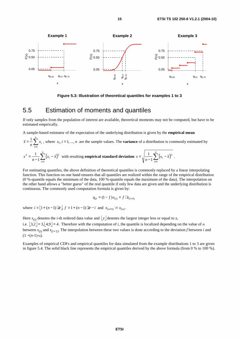
In case of non-symmetric distributed data, moments may not be appropriate for describing the distribution of interest. An alternative measure of location is given by the median, which can be viewed as the point cutting the distribution into halves, namely 50 % of the distribution mass are smaller and 50 % are larger than the median.
More generally, quantiles are defined for each possible percentage. The α-quantile cuts the distribution in a part of α·100 % of the distribution smaller than this value and (1-α)·100 % larger than this value. The median as a special case is also called 50 %-quantile.
A formal definition of quantiles is for instance given by Mood, Graybill, Boes (1974):
• "The α-quantile qα with α ]1,0(∈ is defined as the smallest number q
α satisfying αα ≤)(qF (for α = 0, the
minimum value with positive probability or -∞ is defined, respectively)".
Quantiles are easiest illustrated with the examples of CDFs given above, compare figure 5.3. For each CDF, the 5 %, 50 % and 75 %-quantiles are added to the corresponding plot.
ETSI
ETSI TS 102 250-6 V1.2.1 (2004-10) 15
Example 1
x
F(x
)
q0.05 q0.5, q0.75
0.05
0.50
0.75
Example 2
x
F(x
)
q 0.0
5
q 0.5
q 0.7
5
0.05
0.50
0.75
Example 3
x
F(x
)
q0.05 q0.5 q0.75
0.05
0.50
0.75
Figure 5.3: Illustration of theoretical quantiles for examples 1 to 3
5.5 Estimation of moments and quantiles If only samples from the population of interest are available, theoretical moments may not be computed, but have to be estimated empirically.
A sample-based estimator of the expectation of the underlying distribution is given by the empirical mean
∑=
=n
iix
nx
1
1, where nixi ...,,1, = are the sample values. The variance of a distribution is commonly estimated by
( )∑=
−−
=n
ii xx
ns
1
22
1
1 with resulting empirical standard deviation ( )∑
=
−−
=n
ii xx
ns
1
2
1
1.
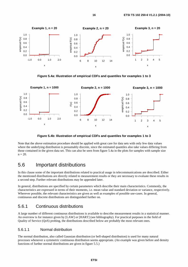
For estimating quantiles, the above definition of theoretical quantiles is commonly replaced by a linear interpolating function. This function on one hand ensures that all quantiles are realized within the range of the empirical distribution (0 %-quantile equals the minimum of the data, 100 %-quantile equals the maximum of the data). The interpolation on the other hand allows a "better guess" of the real quantile if only few data are given and the underlying distribution is continuous. The commonly used computation formula is given by:
)1()()1( +⋅+−= ii xfxfqα
where infni −⋅−+=⋅−+= αα )1(1 ,)1(1 and )()1( : nn xx =+ .
Here x(i) denotes the i-th ordered data value and z denotes the largest integer less or equal to z,
i.e. 49,4,32,3 == . Therefore with the computation of i, the quantile is localized depending on the value of α
between x(i) and x(i+1). The interpolation between these two values is done according to the deviation f between i and (1 +(n-1)·α).
Examples of empirical CDFs and empirical quantiles for data simulated from the example distributions 1 to 3 are given in figure 5.4. The solid black line represents the empirical quantiles derived by the above formula (from 0 % to 100 %).
ETSI
ETSI TS 102 250-6 V1.2.1 (2004-10) 16
Example 1, n = 20
x
empi
rical
F(x
)
-1.0 0.0 1.0 2.0
0.0
0.2
0.4
0.6
0.8
1.0
Example 2, n = 20
x
empi
rical
F(x
)
6 8 10 12 14
0.0
0.2
0.4
0.6
0.8
1.0
Example 3, n = 20
x
empi
rical
F(x
)
1 2 3 4 5
0.0
0.2
0.4
0.6
0.8
1.0
Figure 5.4a: Illustration of empirical CDFs and quantiles for examples 1 to 3
Example 1, n = 1000
x
empi
rica
l F(x
)
-1.0 0.0 1.0 2.0
0.0
0.2
0.4
0.6
0.8
1.0
Example 2, n = 1000
x
F(x
)
6 8 10 12 14
0.0
0.2
0.4
0.6
0.8
1.0
Example 3, n = 1000
xem
piric
al F
(x)
1 2 3 4 5
0.0
0.2
0.4
0.6
0.8
1.0
Figure 5.4b: Illustration of empirical CDFs and quantiles for examples 1 to 3
Note that the above estimation procedure should be applied with great care for data sets with only few data values where the underlying distribution is presumably discrete, since the estimated quantiles also take values differing from those contained in the given data set. This can also be seen from figure 5.4a in the plots for samples with sample size n = 20.
5.6 Important distributions In this clause some of the important distributions related to practical usage in telecommunications are described. Either the mentioned distributions are directly related to measurement results or they are necessary to evaluate these results in a second step. Further relevant distributions may be appended later.
In general, distributions are specified by certain parameters which describe their main characteristics. Commonly, the characteristics are expressed in terms of their moments, i.e. mean value and standard deviation or variance, respectively. Wherever possible, the relevant characteristics are given as well as examples of possible use-cases. In general, continuous and discrete distributions are distinguished further on.
5.6.1 Continuous distributions
A large number of different continuous distributions is available to describe measurement results in a statistical manner. An overview is for instance given by [LAW] or [HART] (see bibliography). For practical purposes in the field of Quality of Service (QoS) probing, the distributions described below are probably the most relevant ones.
5.6.1.1 Normal distribution
The normal distribution, also called Gaussian distribution (or bell-shaped distribution) is used for many natural processes whenever a symmetric continuous distribution seems appropriate. (An example was given before and density functions of further normal distributions are given in figure 5.5.)
ETSI
ETSI TS 102 250-6 V1.2.1 (2004-10) 17
Normal distribution Notation X ~ ),( 2σµN
Parameters σµ,
PDF ( ){ }2
21
21
2exp)( µσπσ
−−= xxf
CDF ( ){ } dttxF
x
∫∞−
−−= 2
21
21
2exp)( µσπσ
Expected value µ=)(XE
Variance 2)( σ=XVar
Remarks Standard normal distribution with 0=µ and 1=σ , see clause 5.6.1.1.1
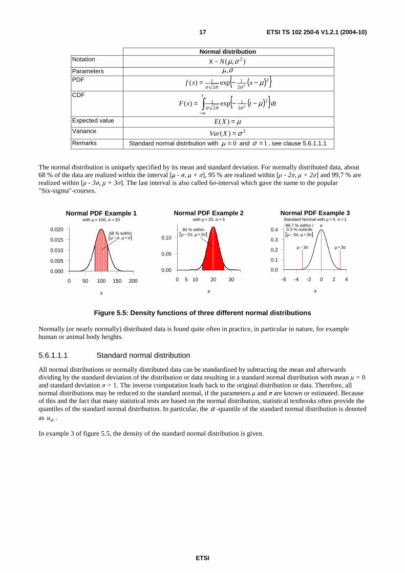
The normal distribution is uniquely specified by its mean and standard deviation. For normally distributed data, about 68 % of the data are realized within the interval [µ - σ, µ + σ], 95 % are realized within [µ - 2σ, µ + 2σ] and 99,7 % are realized within [µ - 3σ, µ + 3σ]. The last interval is also called 6σ-interval which gave the name to the popular "Six-sigma"-courses.
Normal PDF Example 1
x
with µ = 100, σ = 20
68 % within[µ − σ, µ+ σ]
0 50 100 150 200
0.000
0.005
0.010
0.015
0.020
Normal PDF Example 2
x
with µ = 20, σ = 3
95 % within[µ − 2σ, µ +2σ]
0 5 10 20 30
0.00
0.05
0.10
Normal PDF Example 3
x
Standard Normal with µ = 0, σ = 1
µ − 3σ µ +3σ
µ99.7 % within /0.3 % outside[µ − 3σ, µ +3σ]
-6 -4 -2 0 2 4
0.0
0.1
0.2
0.3
0.4
Figure 5.5: Density functions of three different normal distributions
Normally (or nearly normally) distributed data is found quite often in practice, in particular in nature, for example human or animal body heights.
5.6.1.1.1 Standard normal distribution
All normal distributions or normally distributed data can be standardized by subtracting the mean and afterwards dividing by the standard deviation of the distribution or data resulting in a standard normal distribution with mean µ = 0 and standard deviation σ = 1. The inverse computation leads back to the original distribution or data. Therefore, all normal distributions may be reduced to the standard normal, if the parameters µ and σ are known or estimated. Because of this and the fact that many statistical tests are based on the normal distribution, statistical textbooks often provide the quantiles of the standard normal distribution. In particular, the α -quantile of the standard normal distribution is denoted as αu .
In example 3 of figure 5.5, the density of the standard normal distribution is given.
ETSI
ETSI TS 102 250-6 V1.2.1 (2004-10) 18
Standard normal distribution Notation X ~ )1,0(N
Parameters none PDF { }2
21
21 exp)( xxf −=π
CDF { } dttxF
x
∫∞−
−= 221
21 exp)(π
Expected value 0)( =XE
Variance 1)( =XVar
Remarks
5.6.1.1.2 Central limit theorem
Another reason for the frequent use of normal distributions (in particular for testing purposes) is given by the central limit theorem, one of the most important theorems in statistical theory. It states that the mean of n equally distributed random variables with mean µ and variance σ2 approaches a normal distribution with mean µ and variance σ2/n as n becomes larger. This holds for arbitrary distributions and commonly the typical shape of the normal distribution is sufficiently reached for n ≥ 4. For further details about the central limit theorem see [LAW] or [MOOD] (see bibliography).
A number of tools was developed for checking whether data (or means) are normal, namely test procedures like the well-known Kolmogorov-Smirnov goodness-of-fit test (see clause 5.6.6.1.2) among others or graphical tools like histograms or QQ-plots. The mentioned graphical tools will be introduced in clause 6.
5.6.1.1.3 Transformation to normality
As has been seen, the normal distribution is very powerful and can be applied in many situations. Nevertheless, it is not always appropriate, in particular in technical applications, where many parameters of interest have non-symmetric distributions. However, in these situations it may be possible to transform the data to normality. This idea leads for instance to the Log-Normal distribution, which is often assumed for technical parameters.
5.6.1.2 Log-Normal distribution
The distribution of a random variable is said to be Log-Normal, if the logged random variable is normally distributed, which is denoted by log(x) ~ N(µ, σ2).
Log-Normal distribution Notation ),(~ 2σµLNX or ),(~)log( 2σµNX
Parameters σµ,
PDF ( )0 xif
else 02
)ln(exp
2
1)( 2
2
>
−−= σ
µπσ
x
xxf x
CDF
( ){ } dttxF
x
∫∞−
−−= 2
21
21
2exp)( µσπσ
Expected value )
2
1exp()( 2σµ +=xE
Variance )1))(exp(2exp()( 22 −+= σσµxVar
Remarks
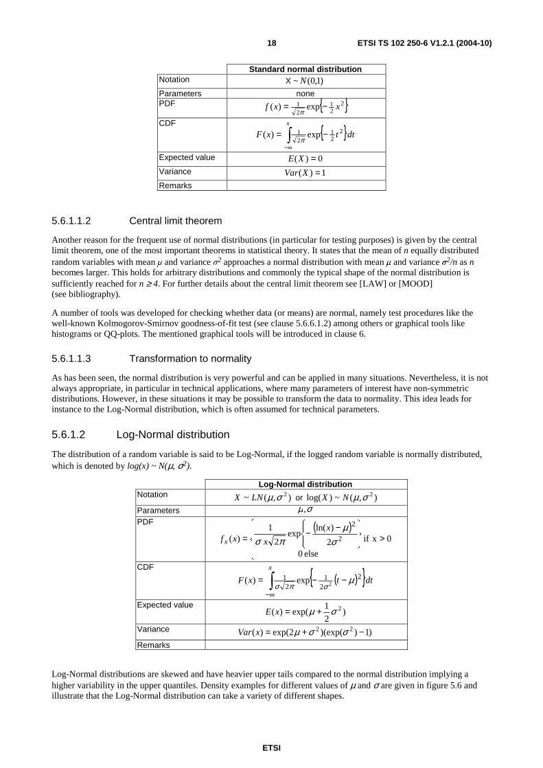
Log-Normal distributions are skewed and have heavier upper tails compared to the normal distribution implying a higher variability in the upper quantiles. Density examples for different values of µ and σ are given in figure 5.6 and illustrate that the Log-Normal distribution can take a variety of different shapes.
ETSI
ETSI TS 102 250-6 V1.2.1 (2004-10) 19
Log-Normal Example 1
x
log(x) is standard normal
0 1 2 3 4 5 6 7
0.00.10.20.30.40.50.6
Log-Normal Example 2
x
log(x) is normal with µ = 2, σ = 0.5
0 5 10 15 20 25 30
0.00
0.05
0.10
Log-Normal Example 3
x
log(x) is normal with µ = 2, σ = 1.5
0 10 20 30 40 50
0.00
0.02
0.04
0.06
0.08
0.10
Figure 5.6: Density functions of Log-Normal distributions
5.6.1.2.1 Use-case: transformations
A given data set can be checked whether it is distributed according to a Log-Normal distribution by computing the log of the data values and using one of the graphical tools mentioned before for verifying the normal distribution for the logged data. Empirical mean and standard deviation of the transformed data can then be used for estimating the parameters of the distribution, respectively.
Similarly, other transformation-based distributions can be derived from the normal distribution, for instance for the
square-root transformation x ~ IN(µ, σ2) or the reciprocal transformation 1/x ~ IN(µ, σ2). A general concept based on power-transformations of x was proposed by Box and Cox (1964).
5.6.1.3 Exponential distribution
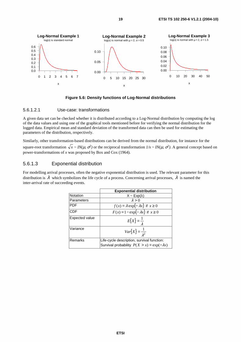
For modelling arrival processes, often the negative exponential distribution is used. The relevant parameter for this distribution is λ which symbolizes the life cycle of a process. Concerning arrival processes, λ is named the inter-arrival rate of succeeding events.
Exponential distribution Notation X ~ Exp(λ) Parameters 0>λ PDF ( )xxf λλ −= exp)( if 0≥x
CDF ( )xxF λ−−= exp1)( if 0≥x
Expected value { }λ1=XE
Variance { }2
1
λ=XVar
Remarks Life-cycle description, survival function: Survival probability )exp()( xxXP λ−=>
ETSI
ETSI TS 102 250-6 V1.2.1 (2004-10) 20
Negative Exponential Example
x
Lambda is 0.5
0 1 2 3 4 5 6 7
0.0
0.1
0.2
0.3
0.4
0.5
0.6
Negative Exponential Example
x
Lambda is 1
0 1 2 3 4 5 6 7
0.0
0.2
0.4
0.6
0.8
1.0
Negative Exponential Example
x
Lambda is 2
0 1 2 3 4 5 6 7
0.0
0.5
1.0
1.5
2.0
Figure 5.7: Density functions of negative exponential distributions
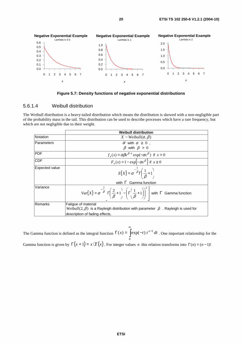
5.6.1.4 Weibull distribution
The Weibull distribution is a heavy-tailed distribution which means the distribution is skewed with a non-negligible part of the probability mass in the tail. This distribution can be used to describe processes which have a rare frequency, but which are not negligible due to their weight.
Weibull distribution Notation ),(~ βαWeibullX
Parameters α with 0≥α , β with 0>β
PDF )exp()( 1 ββ ααβ xxxf x −= − if 0>x
CDF ( )βαxxFx −−= exp1)( if 0≥x
Expected value
{ }
+Γ=
−1
11
βα βXE
with Γ Gamma function Variance
{ }
+Γ−
+Γ=
− 22
11
12
ββα βXVar with Γ Gamma function
Remarks Fatigue of material ),2( βWeibull is a Rayleigh distribution with parameter β . Rayleigh is used for
description of fading effects.
The Gamma function is defined as the integral function ∫∞
−−=Γ0
1)exp()( dtttx x. One important relationship for the
Gamma function is given by ( ) ( )xxx Γ⋅=+Γ 1 . For integer values n this relation transforms into )!1()( −=Γ nn
ETSI
ETSI TS 102 250-6 V1.2.1 (2004-10) 21
Weibull Example 1
x
Weibull data with α = 1 and β = 1
0 1 2 3 4 5 6 7
0.0
0.2
0.4
0.6
0.8
1.0
Weibull Example 2
x
Weibull data with α = 2 and β = 1
0 1 2 3 4 5 6 7
0.0
0.2
0.4
0.6
0.8
1.0
Weibull Example 3
x
Weibull data with α = 3 and β =1
0 1 2 3 4 5 6 7
0.0
0.2
0.4
0.6
0.8
1.0
1.2
Figure 5.8: Density functions of Weibull distributions
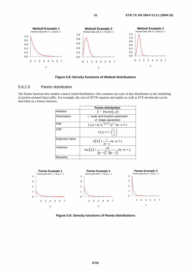
5.6.1.5 Pareto distribution
The Pareto function also models a heavy tailed distribution. One common use-case of this distribution is the modelling of packet-oriented data traffic. For example, the size of HTTP requests and replies as well as FTP downloads can be described as a Pareto function.
Pareto distribution Notation ( )α,~ cParetoX
Parameters c scale and location parameter α shape parameter
PDF ( ) ααα cxxf ⋅⋅= +− 1)( for x c>
CDF
−=x
cxF 1)(
Expected value { }1−
=α
cXE for 1>α
Variance { }( ) ( )21 2 −⋅−
=αα
αcXVar for 2>α
Remarks
Pareto Example 1
x
Pareto data with α = 1 and c = 1
2 3 4 5 6 7
0
1
2
3
4
Pareto Example 2
x
Pareto data with α = 2 and c = 1
2 3 4 5 6 7
0
1
2
3
4
Pareto Example 3
x
Pareto data with α = 4 and c = 1
2 3 4 5 6 7
0
1
2
3
4
Figure 5.9: Density functions of Pareto distributions
ETSI
ETSI TS 102 250-6 V1.2.1 (2004-10) 22
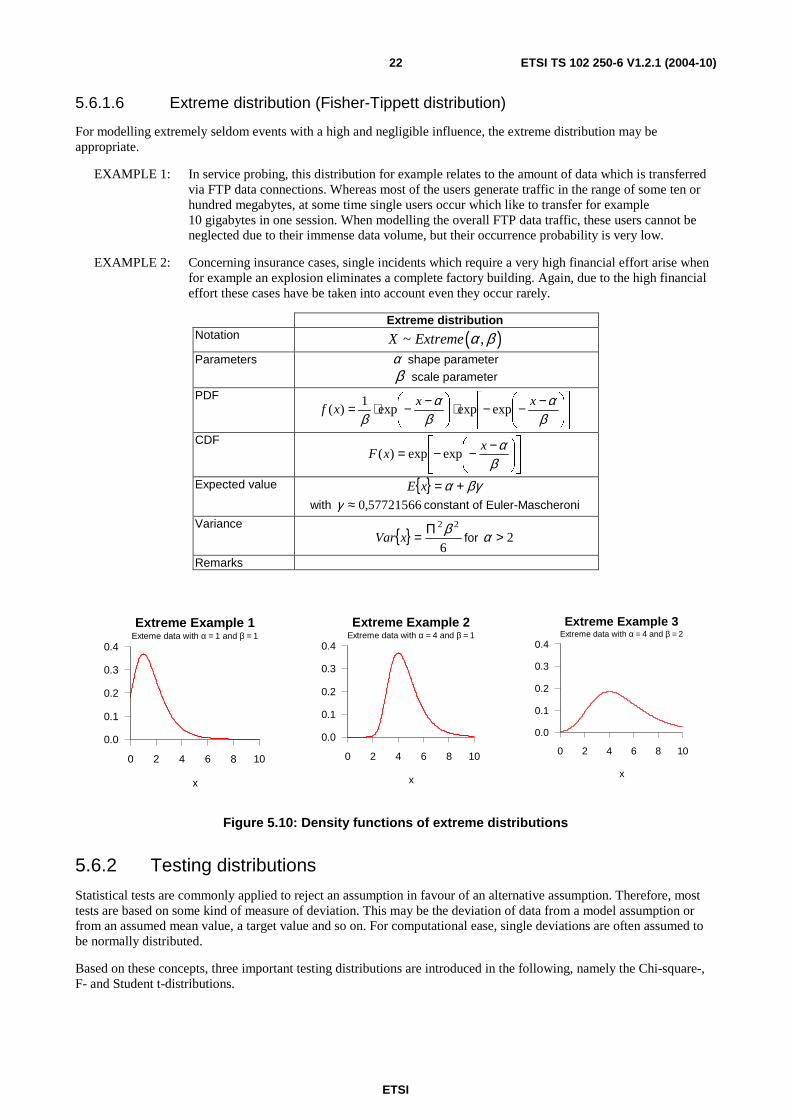
5.6.1.6 Extreme distribution (Fisher-Tippett distribution)
For modelling extremely seldom events with a high and negligible influence, the extreme distribution may be appropriate.
EXAMPLE 1: In service probing, this distribution for example relates to the amount of data which is transferred via FTP data connections. Whereas most of the users generate traffic in the range of some ten or hundred megabytes, at some time single users occur which like to transfer for example 10 gigabytes in one session. When modelling the overall FTP data traffic, these users cannot be neglected due to their immense data volume, but their occurrence probability is very low.
EXAMPLE 2: Concerning insurance cases, single incidents which require a very high financial effort arise when for example an explosion eliminates a complete factory building. Again, due to the high financial effort these cases have be taken into account even they occur rarely.
Extreme distribution Notation ( )~ ,X Extreme α β
Parameters α shape parameter
β scale parameter
−−−⋅
−−⋅=β
αβ
αβ
xxxf expexpexp
1)(
CDF
−−−=β
αxxF expexp)(
Expected value { } βγα +=xE
with 57721566,0≈γ constant of Euler-Mascheroni
Variance { }
6
22βΠ=xVar for 2>α
Remarks
Extreme Example 1
x
Exteme data with α = 1 and β = 1
0 2 4 6 8 10
0.0
0.1
0.2
0.3
0.4
Extreme Example 2
x
Extreme data with α = 4 and β = 1
0 2 4 6 8 10
0.0
0.1
0.2
0.3
0.4
Extreme Example 3
x
Extreme data with α = 4 and β = 2
0 2 4 6 8 10
0.0
0.1
0.2
0.3
0.4
Figure 5.10: Density functions of extreme distributions
5.6.2 Testing distributions
Statistical tests are commonly applied to reject an assumption in favour of an alternative assumption. Therefore, most tests are based on some kind of measure of deviation. This may be the deviation of data from a model assumption or from an assumed mean value, a target value and so on. For computational ease, single deviations are often assumed to be normally distributed.
Based on these concepts, three important testing distributions are introduced in the following, namely the Chi-square-, F- and Student t-distributions.
ETSI
ETSI TS 102 250-6 V1.2.1 (2004-10) 23
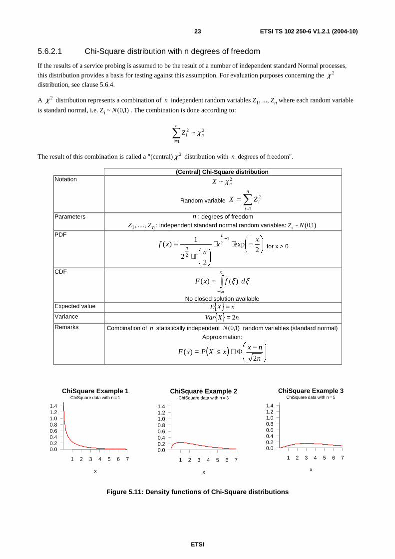
5.6.2.1 Chi-Square distribution with n degrees of freedom
If the results of a service probing is assumed to be the result of a number of independent standard Normal processes,
this distribution provides a basis for testing against this assumption. For evaluation purposes concerning the 2χ
distribution, see clause 5.6.4.
A 2χ distribution represents a combination of n independent random variables Z1, ..., Zn where each random variable
is standard normal, i.e. Zi ~ )1,0(N . The combination is done according to:
2
1
2 ~ n
n
iiZ χ∑
=
The result of this combination is called a "(central) 2χ distribution with n degrees of freedom".
(Central) Chi-Square distribution Notation 2~ nX χ
Random variable ∑=
=n
iiZX
1
2
Parameters n : degrees of freedom
nZZ ....,,1 : independent standard normal random variables: Zi ~ )1,0(N
−⋅⋅
Γ⋅
=−
2exp
22
1)(
12
2
xx
nxf
n
n for x > 0
CDF
ξξ dfxFx
∫∞−
= )()(
No closed solution available Expected value { } nXE =
Variance { } nXVar 2=
Remarks Combination of n statistically independent )1,0(N random variables (standard normal)
Approximation:
( )
−Φ≅≤=n
nxxXPxF
2)(
ChiSquare Example 1
x
ChiSquare data with n = 1
1 2 3 4 5 6 7
0.00.20.40.60.81.01.21.4
ChiSquare Example 2
x
ChiSquare data with n = 3
1 2 3 4 5 6 7
0.00.20.40.60.81.01.21.4
ChiSquare Example 3
x
ChiSquare data with n = 5
1 2 3 4 5 6 7
0.00.20.40.60.81.01.21.4
Figure 5.11: Density functions of Chi-Square distributions
ETSI
ETSI TS 102 250-6 V1.2.1 (2004-10) 24
5.6.2.1.1 Further relations
The referenced gamma function is defined as the integral function:
∫∞
−⋅−=Γ0
1)exp()( dtttx x
Additional useful relations according to this function are:
)()1( xxx Γ⋅=+Γ
and
( )!1)( −=Γ nn if nx = is an integer value
5.6.2.1.2 Relation to empirical variance
• If the mean value µ is known, the empirical variance of n normally distributed random variables reads
( )22
1
1 n
ii
s xnµ µ
=
= ⋅ −∑ . With this piece of information, a chi-square distribution is given for the following
expression: 2
22
~ n
sn µ χ
σ⋅ .
• Without knowledge of µ , the empirical variance ( )22
1
1
1
n
ii
s x xn =
= ⋅ −− ∑ estimates the variance of the
process. The appropriate relation in this case reads ( )2
212
1 ~ n
sn χ
σ −− ⋅ .
5.6.2.2 Student t-distribution
If a standard normal and a statistically independent chi-square distribution with n degrees of freedom are combined
according to
nZ
UX = , where Z ~ χ2 (chi-square distributed) and U ~ N(0,1) (standard normal distributed), the
constructed random variable X is said to be t-distributed with n degrees of freedom. Alternatively, the denomination "Student t-distribution" can be used.
ETSI
ETSI TS 102 250-6 V1.2.1 (2004-10) 25
Student t-distribution Notation
ntX ~
Random variable
nZ
UX = with U ~ N(0,1), Z~χn
2, independent.
Parameters n : degrees of freedom
2
12
1
2
2
1
)(
+−
+⋅
⋅Π⋅
Γ
+Γ=
n
n
x
nn
n
xf
CDF
ξξ dfxFx
∫∞−
= )()(
No closed solution available Expected value 2≥n : { } 0=ZE
Variance 3≥n : { }
2−=
n
nZVar
Remarks The PDF is a symmetric function with symmetry axis 0=x . Additional relation for α -quantiles α;nt : αα −−= 1;; nn tt
Student-t Example 1
x
Student-t data with n = 2
-3 -2 -1 0 1 2 3
0.0
0.1
0.2
0.3
0.4
Student-t Example 2
x
Student-t data with n = 4
-3 -2 -1 0 1 2 3
0.0
0.1
0.2
0.3
0.4
Student-t Example 3
x
Student-t data with n = 40
-3 -2 -1 0 1 2 3
0.0
0.1
0.2
0.3
0.4
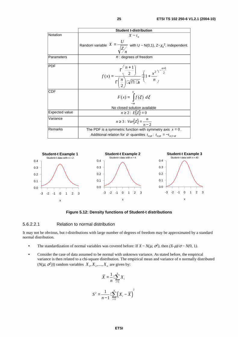
Figure 5.12: Density functions of Student-t distributions
5.6.2.2.1 Relation to normal distribution
It may not be obvious, but t-distributions with large number of degrees of freedom may be approximated by a standard normal distribution.
• The standardization of normal variables was covered before: If X ~ N(µ, σ2), then (X-µ)/σ ~ N(0, 1).
• Consider the case of data assumed to be normal with unknown variance. As stated before, the empirical variance is then related to a chi-square distribution. The empirical mean and variance of n normally distributed (N(µ, σ2))) random variables 1 2, ,..., nX X X are given by:
1
1 n
ii
X Xn =
= ⋅∑
( )2
2
1
1
1
n
ii
S X Xn =
= ⋅ −− ∑
ETSI
ETSI TS 102 250-6 V1.2.1 (2004-10) 26
With these relations, the relation between the t-distribution and the n normal distributed random variables reads:
12~ n
Xn t
S
µ−
−⋅ .
5.6.2.3 F distribution
The F distribution is a combination of m standard normal distributed random variables iY and n standard normal
distributed random variables Vi which are combined as described below. Again, m and n are called "degrees of freedom" of this distribution.
This distribution is often used for computation and evaluation purposes, for example in relation with confidence intervals for the binomial distribution (Pearson-Clopper formula). In general, it compares two types of deviations, for instance if two different models are fitted.
F distribution Notation
nmFX ,~
Random variable
∑
∑
=
=
⋅
⋅
=n
i
i
m
i
i
Vn
Ym
X
1
2
1
2
1
1
Parameters nm, : degrees of freedom
nYY ,....,1 : independent random variables according to )1,0(N
nVV ,....,1 : independent random variables according to )1,0(N
2
122
1
2,
2
)(
nm
mm
xn
m
nmB
xn
m
xf
+−−
⋅+⋅
⋅
= for 0>x
with ( ))()()(
,qp
qpqpB
+ΓΓ⋅Γ=
Eularian beta function CDF
ξξ dfxFx
∫∞−
= )()(
No closed solution available Expected value
2>n : { }2−
=n
nZE
Variance 4>n : { } ( )
( ) ( )42
222
2
−−−+=
nnm
mmnZVar
Remarks A nmF , related distribution can be interpreted as the quotient of a 2mχ
distribution and a 2nχ distribution multiplied with
m
n .
ETSI
ETSI TS 102 250-6 V1.2.1 (2004-10) 27
F Example 1
x
F data with m = 4 and n = 40
0 1 2 3 4 5 6 7
0.0
0.2
0.4
0.6
0.8
1.0
F Example 2
x
F data with m = 2 and n = 2
0 1 2 3 4 5 6 7
0.0
0.2
0.4
0.6
0.8
1.0
F Example 3
x
F data with m = 40 and n = 4
0 1 2 3 4 5 6 7
0.0
0.2
0.4
0.6
0.8
1.0
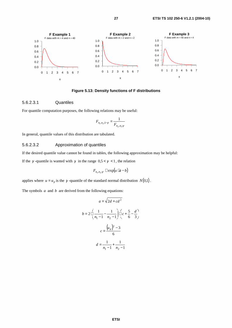
Figure 5.13: Density functions of F distributions
5.6.2.3.1 Quantiles
For quantile computation purposes, the following relations may be useful:
γ
γ;,
1;,12
21
1
nnnn F
F =−
In general, quantile values of this distribution are tabulated.
5.6.2.3.2 Approximation of quantiles
If the desired quantile value cannot be found in tables, the following approximation may be helpful:
If the γ -quantile is wanted with γ in the range 15,0 << γ , the relation
( )bauF nn −⋅≅ exp;, 21 γ
applies where γuu = is the γ -quantile of the standard normal distribution ( )1,0N .
The symbols a and b are derived from the following equations:
22 cdda +=
−+⋅
−−
−⋅=
36
5
1
1
1
12
21
dc
nnb
( )
6
32 −= γu
c
1
1
1
1
21 −+
−=
nnd
ETSI
ETSI TS 102 250-6 V1.2.1 (2004-10) 28
5.6.2.3.3 Relations to other distributions
When the F distribution comes to usage, the following relations may ease the handling of this distribution:
• Relation to t distribution for 11 =n :
2
2
1;
;,12
2
= +γγ
nn tF .
• Relation to 2χ distribution for ∞→2n : 2;
1;, 11
1γγ χ nn n
F ⋅=∞ .
• If ∞→1n and ∞→2n , the distribution simplifies to: 1;, =∞∞ γF
5.6.3 Discrete distributions
Discrete distributions describe situations where the outcome of measurements is restricted to integer values. For example, the results of service access tests show either that service access is possible (mostly represented by a logical "1" value) or that it is not possible (mostly represented by a logical "0" value). Depending on the circumstances under which such "drawing a ball out of a box" tests are executed, different statistical distributions apply like shown in clauses 5.6.3.1 to 5.6.3.4.
5.6.3.1 Bernoulli distribution
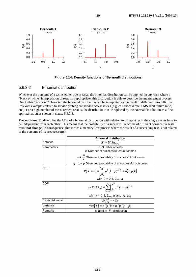
The starting point of different discrete distributions is given by the Bernoulli distribution. It simply describes the probability p of a positive outcome of a single test where only two states are allowed, generally a positive one and a
negative one. As soon as more than one single test is executed, further discrete distribution may be applied as shown in the following clauses.
Bernoulli distribution Notation )(~ pBernoulliX
Parameters ( )1,0∈p
==−
= otherwise 0
1 xif
0 xif 1
)( p
p
xp
CDF
≤<≤−
<=
x 1 if 1
1 x0 if 1
0 xif 0
)( pxF
Expected value { } pXE =
Variance { } ( )ppXVar −⋅= 1
Remarks
ETSI
ETSI TS 102 250-6 V1.2.1 (2004-10) 29
Bernoulli 1
x
f(x)
p is 0.8
-1.0 0.0 1.0 2.0
0.0
0.2
0.4
0.6
0.8
1.0
Bernoulli 2
x
f(x)
p is 0.6
-1.0 0.0 1.0 2.0
0.0
0.2
0.4
0.6
0.8
1.0
Bernoulli 3
x
f(x)
p is 0.3
-1.0 0.0 1.0 2.0
0.0
0.2
0.4
0.6
0.8
1.0
Figure 5.14: Density functions of Bernoulli distributions
5.6.3.2 Binomial distribution
Whenever the outcome of a test is either true or false, the binomial distribution can be applied. In any case where a "black or white" interpretation of results is appropriate, this distribution is able to describe the measurement process. Due to this "yes or no" character, the binomial distribution can be interpreted as the result of different Bernoulli tries. Relevant examples related to service probing are service access issues (e.g. call success rate, SMS send failure ratio, etc.). For a high number of measurement results, the distribution can be replaced by the Normal distribution as a first approximation as shown in clause 5.6.3.3.
Precondition: To determine the CDF of a binomial distribution with relation to different tests, the single events have to be independent from each other. This means that the probability of a successful outcome of different consecutive tests must not change. In consequence, this means a memory-less process where the result of a succeeding test is not related to the outcome of its predecessor(s).
Binomial distribution Notation ( )pnBinX ,~
Parameters n Number of tests m Number of successful test outcomes
n
mp = Observed probability of successful outcomes
pq −=1 Observed probability of unsuccessful outcomes
PDF ( )kpnbpp
k
nkXP knk ,,)1()( =−
== −
with nk ,...,2,1,0=
CDF
∑=
−−
=≤
0
00 )1()(
k
k
knk ppk
nkXP
with nk ,...,2,1,0= and kk ≥0
Expected value { } pnXE ⋅=
Variance { } )1( ppnqpnXVar −⋅⋅=⋅⋅=
Remarks Related to F distribution
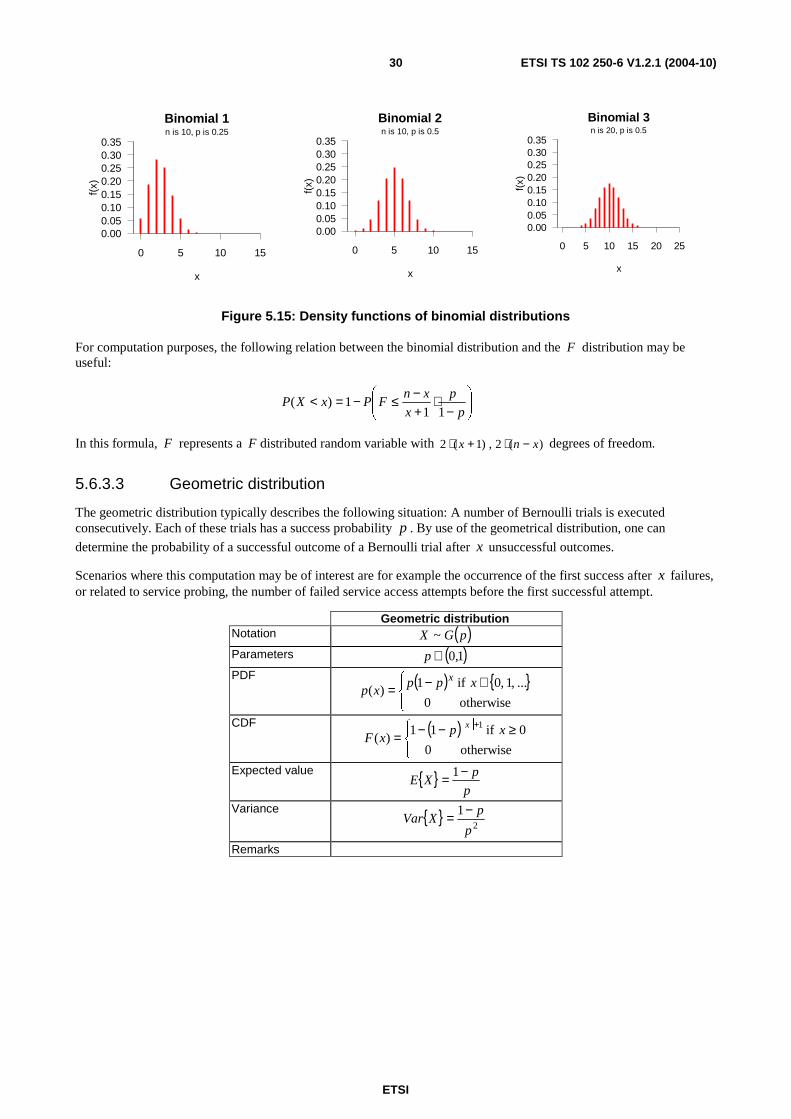
ETSI
ETSI TS 102 250-6 V1.2.1 (2004-10) 30
Binomial 1
x
f(x)
n is 10, p is 0.25
0 5 10 15
0.000.050.100.150.200.250.300.35
Binomial 2
x
f(x)
n is 10, p is 0.5
0 5 10 15
0.000.050.100.150.200.250.300.35
Binomial 3
x
f(x)
n is 20, p is 0.5
0 5 10 15 20 25
0.000.050.100.150.200.250.300.35
Figure 5.15: Density functions of binomial distributions
For computation purposes, the following relation between the binomial distribution and the F distribution may be useful:
−⋅
+−≤−=<
p
p
x
xnFPxXP
111)(
In this formula, F represents a F distributed random variable with )(2,)1(2 xnx −⋅+⋅ degrees of freedom.
5.6.3.3 Geometric distribution
The geometric distribution typically describes the following situation: A number of Bernoulli trials is executed consecutively. Each of these trials has a success probability p . By use of the geometrical distribution, one can
determine the probability of a successful outcome of a Bernoulli trial after x unsuccessful outcomes.
Scenarios where this computation may be of interest are for example the occurrence of the first success after x failures, or related to service probing, the number of failed service access attempts before the first successful attempt.
Geometric distribution Notation ( )pGX ~
Parameters ( )1,0∈p
PDF ( ) { }
∈−=
otherwise 0
...,1,0 if 1)(
xppxp
x
CDF ( )
≥−−=
+
otherwise 0
0 if 11)(
1 xpxF
x
Expected value { }p
pXE
−= 1
Variance { }2
1
p
pXVar
−=
Remarks
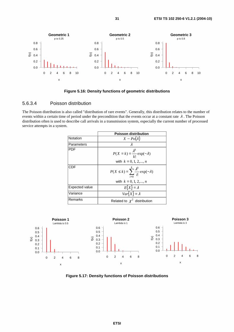
ETSI
ETSI TS 102 250-6 V1.2.1 (2004-10) 31
Geometric 1
x
f(x)
p is 0.25
0 2 4 6 8 10
0.0
0.2
0.4
0.6
0.8
Geometric 2
x
f(x)
p is 0.5
0 2 4 6 8 10
0.0
0.2
0.4
0.6
0.8
Geometric 3
x
f(x)
p is 0.8
0 2 4 6 8 10
0.0
0.2
0.4
0.6
0.8
Figure 5.16: Density functions of geometric distributions
5.6.3.4 Poisson distribution
The Poisson distribution is also called "distribution of rare events". Generally, this distribution relates to the number of events within a certain time of period under the precondition that the events occur at a constant rate λ . The Poisson distribution often is used to describe call arrivals in a transmission system, especially the current number of processed service attempts in a system.
Poisson distribution Notation ( )λPoX ~
Parameters λ PDF
)exp(!
)( λλ −==k
kXPk
with nk ,...,2,1,0=
CDF
∑=
−=≤k
i
k
ikXP
0
)exp(!
)( λλ
with nk ,...,2,1,0=
Expected value { } λ=XE
Variance { } λ=XVar
Remarks Related to 2χ distribution
Poisson 1
x
f(x)
Lambda is 0.5
0 2 4 6 8
0.00.10.20.30.40.50.6
Poisson 2
x
f(x)
Lambda is 1
0 2 4 6 8
0.00.10.20.30.40.50.6
Poisson 3
x
f(x)
Lambda is 3
0 2 4 6 8
0.00.10.20.30.40.50.6
Figure 5.17: Density functions of Poisson distributions
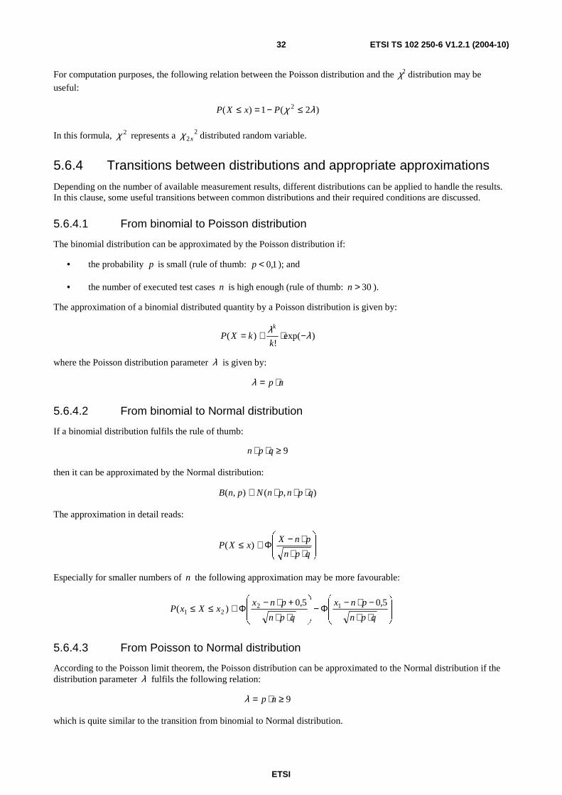
ETSI
ETSI TS 102 250-6 V1.2.1 (2004-10) 32
For computation purposes, the following relation between the Poisson distribution and the 2χ distribution may be
useful:
)2(1)( 2 λχ ≤−=≤ PxXP
In this formula, 2χ represents a 22xχ distributed random variable.
5.6.4 Transitions between distributions and appropriate approximations
Depending on the number of available measurement results, different distributions can be applied to handle the results. In this clause, some useful transitions between common distributions and their required conditions are discussed.
5.6.4.1 From binomial to Poisson distribution
The binomial distribution can be approximated by the Poisson distribution if:
• the probability p is small (rule of thumb: 1,0<p ); and
• the number of executed test cases n is high enough (rule of thumb: 30>n ).
The approximation of a binomial distributed quantity by a Poisson distribution is given by:
)exp(!
)( λλ −⋅≅=k
kXPk
where the Poisson distribution parameter λ is given by:
np ⋅=λ
5.6.4.2 From binomial to Normal distribution
If a binomial distribution fulfils the rule of thumb:
9≥⋅⋅ qpn
then it can be approximated by the Normal distribution:
),(),( qpnpnNpnB ⋅⋅⋅≅
The approximation in detail reads:
⋅⋅⋅−Φ≅≤qpn
pnXxXP )(
Especially for smaller numbers of n the following approximation may be more favourable:
⋅⋅−⋅−
Φ−
⋅⋅+⋅−
Φ≅≤≤qpn
pnx
qpn
pnxxXxP
5,05,0)( 12
21
5.6.4.3 From Poisson to Normal distribution
According to the Poisson limit theorem, the Poisson distribution can be approximated to the Normal distribution if the distribution parameter λ fulfils the following relation:
9≥⋅= npλ
which is quite similar to the transition from binomial to Normal distribution.
ETSI
ETSI TS 102 250-6 V1.2.1 (2004-10) 33
Then, the approximation reads:
−Φ≅≤λλk
kXP )(
5.6.5 Truncated distributions
According to resource constraints of measurement equipment, some measurements have to consider timeout values. By the use of timeouts, the maximal period of time in which measurement results are considered as relevant for the measurement is limited. The resulting density function then is clipped at the right-hand side. Truncation may also occur at both ends of a density function.
For example, if the end-to-end delivery time of some message service is subject of a measurement, the introduction of timeout values may reduce the number of measurement samples. This is because all delivery times which are higher than the defined timeout value are discarded. By discarding some samples, the entirety of data is reduced which means that probabilities describing the measurement may be influenced.
In general, truncation can be described by conditional probabilities. The condition is given by the timeout value. Furthermore, probabilities are then computed under the constraint of the timeout. Truncated Normal and Poisson distributions are covered in more detail by [MOOD] (see bibliography).
5.6.6 Distribution selection and parameter estimation
If a distribution is sought to describe a given data set, two steps have to be carried out. Firstly, an appropriate distribution family (type of distribution) has to be selected and secondly, the corresponding parameters specifying this distribution have to be estimated. Test procedures or graphical methods may be applied for the first step, parameter estimation procedures are needed for the second.
5.6.6.1 Test procedures
The formulation of tests is covered in detail in clause 5.7.1. In this clause, three well-known tests that may be used for checking distributional assumptions are described briefly. It focuses mainly on the fundamental ideas leading to these tests.
All test procedures are based on comparisons between assumed and empirical distribution. That is, from the data on hand, the underlying distribution is guessed and then verified by applying one of the test procedures described in clauses 5.6.6.1.1 to 5.6.6.1.3.
5.6.6.1.1 Chi-Square test
The main idea of the Chi-Square test is to test whether a set of data comes from a normal distribution by building classes and checking whether the expected number of observations and the number of data in each class are similar. If the deviations between both numbers - in terms of squared differences - exceeds a corresponding χ2-value, the distribution assumed has to be rejected.
5.6.6.1.2 Kolmogorov-Smirnov test
The Kolmogorov-Smirnov test is based on the cumulative distribution functions of the theoretical (assumed) and empirical distribution of the data at hand. The main idea is that the distributional assumption is rejected, if the maximum vertical distance between both Cumulative Density Functions (CDFs) exceeds a critical value.
5.6.6.1.3 Shapiro-Wilk test
Shapiro and Wilk suggested a test procedure that is based on quantiles and related to the QQ-Plot introduced in clause 6. The main idea of this test is to compare the sum of squared deviations between the points of the QQ-Plot and the best fitting straight line with a given χ2-value.
ETSI
ETSI TS 102 250-6 V1.2.1 (2004-10) 34
5.6.6.2 Parameter estimation methods
Most frequently applied methods for parameter estimation are Maximum-Likelihood or Moment estimation methods. For the mean of a normal distribution, both methods yield identical results. For further details compare [MOOD] (see bibliography).
5.7 Evaluation of measurement data Related to active service probing, certain issues can become much easier to handle if it is able to describe the gathered data in a very compact way. One possible way to reach this aim is to execute different tests and thereby to check some assumptions. These assumptions are stated before any testing is done. They are called "hypotheses".
From a slightly more theoretical point of view, this topic can be expressed as follows:
With every measurement sample some information about the investigated process is retrieved. Since commonly the characteristics of the process are unknown, with every piece of additional information (i.e. every sample) the degree of knowledge increases. This knowledge is formalized by the application of statistical tests or the determination of confidence intervals for the distributional parameters of interest.
The idea of statistical tests and some simple examples are presented in clause 5.7.1. Subsequently, the construction of confidence intervals and the relation between test and confidence intervals will be covered in clause 5.7.2.
5.7.1 Statistical tests
Statistical tests are introduced by specifying the test components first and afterward distinguishing different test classes and giving examples where appropriate.
5.7.1.1 Formulation of statistical tests
Statistical tests are formulated by specifying the following components:
• (Null-)Hypothesis: This hypothesis is commonly denoted by H or H0.
EXAMPLE 1: H: µ = 60.
• Alternative Hypothesis: This one is commonly denoted by A or H1.
EXAMPLE 2: A: 60µ ≠ or A: µ > 60.
• Test statistic: A test statistic is derived so that it is sensitive for deviation from the hypothesis in favour of the alternative. That is, the meaning of the test statistic is to notice if in fact A is true instead of H. Test statistics are commonly denoted by T.
• Testing rule and critical value: The testing rule states the condition under which H is rejected in favour of the alternative A. So it represents something like a switching condition.
EXAMPLE 3: "Reject H, if x c> " or "Reject H, if x c> ".
The value c is called "critical value".
• Type I: Error level α : The probability of rejection H, although true, is controlled by the value α . The specification of α has direct impact on c and thereby on the testing rule. Commonly, the type I error is restricted to 5 % or 1 %, that is α = 0,05 or α = 0,01, respectively.
A statistical test is carried out by specifying all of the above components, computing the test statistic and comparing it with the critical value. Test results are usually documented by reporting the value of the test statistic as well as the corresponding test result. Alternatively, the so called p-value may be reported. This value measures the "significance" or a test result in the way that if the p-value is smaller than the error level α , the hypothesis is rejected, otherwise it may not be rejected. A p-value corresponds to the smallest α -level for which the test would have been rejected.
ETSI
ETSI TS 102 250-6 V1.2.1 (2004-10) 35
5.7.1.2 Classes of statistical tests
Commonly, statistical tests are formulated in the way that the alternative makes the statement one wishes to prove in a statistical sense. That is, in general tests seek to reject a given hypothesis and are therefore formulated accordingly. This is done due to the fact that if the Type I error is specified, a rejection implies that the hypothesis is untrue with user-defined certainty.
However, a number of test procedures exist that differ from the mentioned general test philosophy. Some of these examples are the tests used for selecting distributions (compare clause 5.6.6). Their purpose is to support the hypothesis. Nevertheless, strictly speaking it is impossible to proof any equality hypothesis, therefore the test result can either be that there is no hint that the hypothesis is violated or that there is evidence that the assumed distribution is not appropriate. In the following, it is assumed that one wishes to reject the hypothesis in favour of the alternative.
Two major classes of tests are distinguished, namely one-sample and two-sample tests.
• If a test is based on only one data set for which a reference alternative is to be checked, this is a one-sample test.
• On the other hand, two data sets may be compared by testing for instance the hypothesis H related to the Multimedia Messaging Service (MMS).
H: MMS-E2E-Delivery Time [this week] > MMS-E2E-Delivery Time [last week]
against the alternative that the MMS-E2E-Delivery Time was reduced from last week to this week.
Furthermore, tests that are based on distributional assumptions and distribution-free tests are distinguished. Most distribution-based tests are testing for the location and dispersion / variation of an assumed distribution. For two-sample tests, both samples are assumed to be from the same type of distribution, but possibly with different parameters, for instance different location. In contrast, distribution-free tests should be applied, if there is not enough knowledge about the distribution of the data. However, distribution-free tests are in general less powerful, therefore distribution-based tests should be preferred, if appropriate.
5.7.1.3 Tests for normal and binomial data
In the following clauses, two of the main use-cases of statistical data are taken into concern. These clauses deal with test for normal distributed and binomial distributed data.
5.7.1.3.1 One-sample tests for normal data
If data are from a normal distribution with known variance 20σ , i.e. 2
1 0,..., ~ ( , )nX X N µ σ , three different
location tests may be carried out. All of these compare the location of a given sample to a value µ0, that may be chosen arbitrarily.
• Test for H: µ = µ0 vs. A: µ ≠ µ0: The corresponding test statistic is given by 0
x µT n
σ−=
H is rejected, if T > u1-α/2.
• Test for H: µ ≤ µ0 vs. A: µ >µ0: The corresponding test statistic is given by 0
0
x µT n
σ−
=
H is rejected, if T > u1-α (for α < 0,5).
• Test for H: µ ≥ µ0 vs. A: µ <µ0: The corresponding test statistic is again given by 0
0
x µT n
σ−
=
H is rejected, if T < uα = − u1−α (for α < 0,5).
ETSI
ETSI TS 102 250-6 V1.2.1 (2004-10) 36
If data are from a normal distribution, but the variance is unknown, i.e. 21,..., ~ ( , )nX X N µ σ , the variance has to
be estimated from the data and the above "normal-tests" are replaced by student t-tests. In this case, the variance estimator:
( )22
1
1
1
n
ii
s x xn =
= −− ∑
is applied. Test statistics are replaced as follows: 0x µT n
S
−= or 0
0
x µT n
σ−
= , respectively. Critical values are
given by the quantiles of the t-distribution: tn-1, 1-α/2 , tn-1, 1-α or tn-1, α, respectively.
If instead the variance is unknown and subject of a test, i.e. 21,..., ~ ( , )nX X N µ σ with unknown µ and σ2, the
following tests comparing the variance of a given sample to a value 0σ , that may be carried out.
• Test for H: σ = σ0 vs. A: σ ≠ σ0: The corresponding test statistic is given by T = (n-1)/σ0 2 s2 with
( )22
1
1
1
n
ii
s x xn =
= −− ∑ . H is rejected, if T > χ2
1-α/2, n-1 or T < χ2α/2, n-1.
• Test for H: σ ≤ σ 0 vs. A: σ >σ 0: The corresponding test statistic is again given by T = (n-1)/σ02 s2 with s2 as
given above. H is rejected, if T > χ21-α,, n-1.
• Test for H: σ ≥ σ 0 vs. A: σ <σ 0: Test statistic and empirical variance are as before. In this case, H is rejected,
if T < χ2α,, n-1.
5.7.1.3.2 Two-sample tests for normal data
In the case of two samples, that are to be compared, two very different situations are distinguished. The two samples can either be collected on the same observational units or can be observed independently. If both samples are from the same units, for example measuring the cut-of-call-ratio at different network elements before and after a new piece of software is installed, the two samples are called paired and two observations from the same unit will generally be correlated. In this case, the differences between both measurements for each unit are computed and the new observations Di = Xi - Yi are assumed to be normal with expectation µD = µ X − µY . Then, the above tests for normal
data may be applied, for instance to test for µD=0, i.e. µ X =µY to prove that there is a significant difference between
both samples.
For independent data from two samples, both assumed to be normally distributed with the same known variance,
but possibly different expectations, i.e. 21,..., ~ ( , )n XX X N µ σ and 2
1,..., ~ ( , )m YY Y N µ σ , tests to compare both
means are given as follows.
The following test statistic T is defined for testing the hypotheses:
mn
yxT
11 +
−=σ
• Test for H: µX = µY vs. A: µX ≠ µY: H is rejected, if |T| > u1-α/2
• Test for H: µX ≤ µY vs. A: µX > µY: H is rejected, if T > u1-α
• Test for H: µX ≥ µY vs. A: µX < µY: H is rejected, if T < uα
If the variance is unknown but assumed to be equal for both samples, the normal distribution is again replaced by a Student t-distribution resulting in the following test procedures.
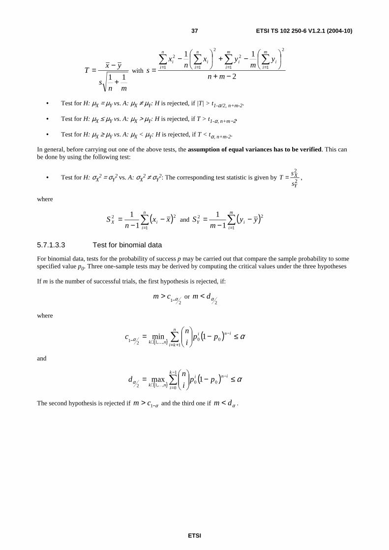
ETSI
ETSI TS 102 250-6 V1.2.1 (2004-10) 37
mns
yxT
11 +
−= with 2
112
11
2
2
11
2
−+
−+
−=
∑∑∑∑====
mn
ym
yxn
x
s
m
ii
m
ii
n
ii
n
ii
• Test for H: µX = µY vs. A: µX ≠ µY: H is rejected, if |T| > t1-α/2, n+m-2.
• Test for H: µX ≤ µY vs. A: µX > µY: H is rejected, if T > t1-α, n+m−2.
• Test for H: µX ≥ µY vs. A: µX < µY: H is rejected, if T < tα, n+m-2.
In general, before carrying out one of the above tests, the assumption of equal variances has to be verified. This can be done by using the following test:
• Test for H: σX2 = σY
2 vs. A: σX2 ≠ σY
2: The corresponding test statistic is given by 2
2
Y
X
s
sT = ,
where
( )∑=
−−
=n
iiX xx
nS
1
22
1
1 and ( )∑
=
−−
=m
iiY yy
mS
1
22
1
1
5.7.1.3.3 Test for binomial data
For binomial data, tests for the probability of success p may be carried out that compare the sample probability to some specified value p0. Three one-sample tests may be derived by computing the critical values under the three hypotheses
If m is the number of successful trials, the first hypothesis is rejected, if:
21 α−
> cm or 2
αdm <
where
{ }
( ) αα ≤−
= −
+=∈− ∑ini
n
kink
ppi
nc 00
1,,121
1minK
and
{ }
( ) αα ≤−
= −
−
=∈ ∑ini
k
ink
ppi
nd 00
1
0,,12
1maxK
The second hypothesis is rejected if α−> 1cm and the third one if αdm < .
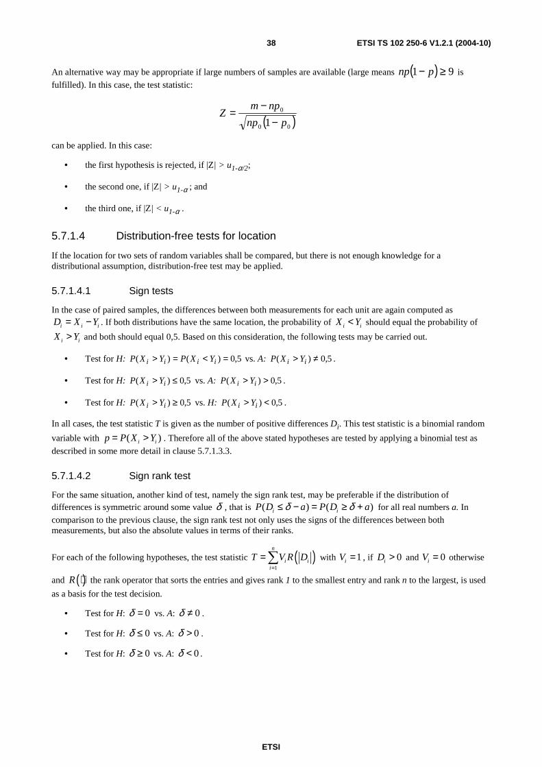
ETSI
ETSI TS 102 250-6 V1.2.1 (2004-10) 38
An alternative way may be appropriate if large numbers of samples are available (large means ( ) 91 ≥− pnp is
fulfilled). In this case, the test statistic:
( )00
0
1 pnp
npmZ
−−
=
can be applied. In this case:
• the first hypothesis is rejected, if |Z| > u1-α/2;
• the second one, if |Z| > u1-α ; and
• the third one, if |Z| < u1-α .
5.7.1.4 Distribution-free tests for location
If the location for two sets of random variables shall be compared, but there is not enough knowledge for a distributional assumption, distribution-free test may be applied.
5.7.1.4.1 Sign tests
In the case of paired samples, the differences between both measurements for each unit are again computed as
i i iD X Y= − . If both distributions have the same location, the probability of i iX Y< should equal the probability of
i iX Y> and both should equal 0,5. Based on this consideration, the following tests may be carried out.
• Test for H: 5,0)()( =<=> iiii YXPYXP vs. A: 5,0)( ≠> ii YXP .
• Test for H: 5,0)( ≤> ii YXP vs. A: 5,0)( >> ii YXP .
• Test for H: 5,0)( ≥> ii YXP vs. H: 5,0)( <> ii YXP .
In all cases, the test statistic T is given as the number of positive differences Di. This test statistic is a binomial random
variable with ( )i ip P X Y= > . Therefore all of the above stated hypotheses are tested by applying a binomial test as
described in some more detail in clause 5.7.1.3.3.
5.7.1.4.2 Sign rank test
For the same situation, another kind of test, namely the sign rank test, may be preferable if the distribution of differences is symmetric around some value δ , that is ( ) ( )i iP D a P D aδ δ≤ − = ≥ + for all real numbers a. In
comparison to the previous clause, the sign rank test not only uses the signs of the differences between both measurements, but also the absolute values in terms of their ranks.
For each of the following hypotheses, the test statistic ( )1
n
i ii
T V R D=
=∑ with 1iV = , if 0iD > and 0iV = otherwise
and ( )R ⋅ the rank operator that sorts the entries and gives rank 1 to the smallest entry and rank n to the largest, is used
as a basis for the test decision.
• Test for H: 0δ = vs. A: 0δ ≠ .
• Test for H: 0δ ≤ vs. A: 0δ > .
• Test for H: 0δ ≥ vs. A: 0δ < .
ETSI
ETSI TS 102 250-6 V1.2.1 (2004-10) 39
For the test statistic, we have a distribution with expectation ( ) ( )11
4E T n n= + and variance
( ) ( )( )11 2 1
24Var T n n n= + + . The quantiles of the resulting distribution are given in statistical text books on
nonparametric methods. However, in case 20n ≥ , the distribution of ( )( )
T E T
Var T
− may be approximated by a standard
normal distribution.
5.7.1.4.3 Wilcoxon rank sum test
In contradiction to both tests explained before, the rank sum test suggested by Wilcoxon is used for independent samples. It assumes that both samples come from the same kind of distribution, but with a shifted location, that is
1,..., nX X and 1,..., mY Y ( n m≤ ) are independent and have continuous distribution functions XF and YF respectively.
These are shifted by δ , i.e. ( ) ( )X YF x F x δ= + . Meaningful hypotheses are the following:
• Test for H: 0δ = vs. A: 0δ ≠ .
• Test for H: 0δ ≤ vs. A: 0δ > .
• Test for H: 0δ ≥ vs. A: 0δ < .
In this situation, for instance a rejection of the third hypothesis, i.e. 0δ < would imply that the location of the second distribution function is significantly smaller, that is the y-values are in general be smaller than the x-values.
For the above tests, a sensible test statistic is derived by combining both data sets to one sample and computing ranks by ordering the values according to their size. The test statistic T is now given by the sum of all ranks for values from the first sample, i.e. the x-values. For this test statistic, expectation and variance are given by:
( ) ( )11
2E T n n m= + +
and
( ) ( )11
12Var T n m n m= + +
respectively. Again, exact critical values for these tests are not easy to derive, but approximations exist. If , 4n m ≥ and
30n m+ ≥ , the distribution of ( )( )
T E T
Var T
− may be approximated by a standard normal distribution.
5.7.2 Confidence interval
In contrast to point estimators where a single number is used to summarize measurement data (compare methods for estimating moments or quantiles in clause 5.5), confidence intervals describe an interval that covers the true parameter value with a certain probability. Usual probability measures are in the 90 percent range. For example, a confidence interval represents the interval in which the mean of the underlying distribution lies with a probability of 95 percent or with a probability of 99 percent.
Confidence intervals are related to statistical tests in the sense that a confidence interval with a given confidence level, for instance 95 %, contains all Confidence levels are denoted by 1-α, where α corresponds to the Type I error level for tests.
As a rule of thumb the number of samples within a measurement campaign correlate with the reliability of results. In other word: The higher the number of collected samples, the more precise and trustworthy the results are.
The computation of confidence intervals depends heavily on the assumed kind of distribution. In the following, the computation of confidence intervals is described for the binomial and the normal (Gaussian) distribution.
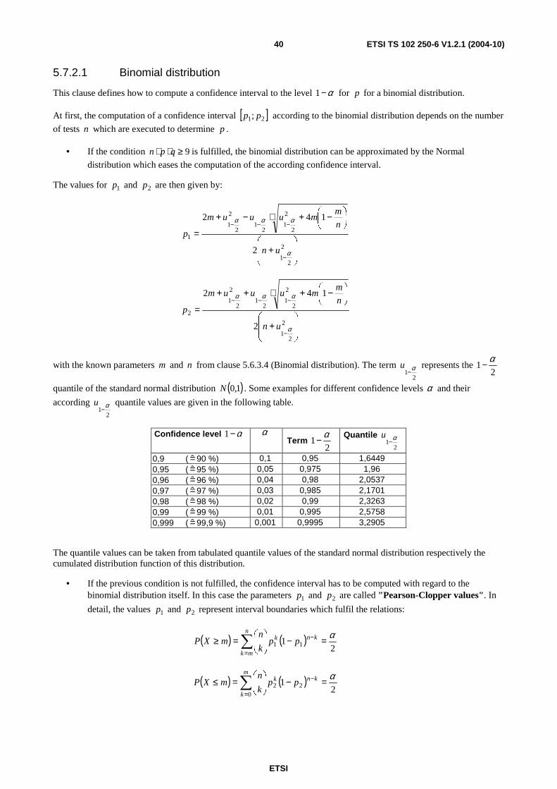
ETSI
ETSI TS 102 250-6 V1.2.1 (2004-10) 40
5.7.2.1 Binomial distribution
This clause defines how to compute a confidence interval to the level α−1 for p for a binomial distribution.
At first, the computation of a confidence interval [ ]21; pp according to the binomial distribution depends on the number
of tests n which are executed to determine p .
• If the condition 9≥⋅⋅ qpn is fulfilled, the binomial distribution can be approximated by the Normal
distribution which eases the computation of the according confidence interval.
The values for 1p and 2p are then given by:
+
−+⋅−+
=
−
−−−
2
21
2
21
21
2
21
1
2
142
α
ααα
un
n
mmuuum
p
+
−+⋅++
=
−
−−−
2
21
2
21
21
2
21
2
2
142
α
ααα
un
n
mmuuum
p
with the known parameters m and n from clause 5.6.3.4 (Binomial distribution). The term 2
1α−
u represents the 2
1α−
quantile of the standard normal distribution ( )1,0N . Some examples for different confidence levels α and their
according 2
1α−
u quantile values are given in the following table.
Confidence level α−1 α Term
21
α− Quantile
21
α−u
0,9 ( =̂ 90 %) 0,1 0,95 1,6449 0,95 ( =̂ 95 %) 0,05 0,975 1,96 0,96 ( =̂ 96 %) 0,04 0,98 2,0537 0,97 ( =̂ 97 %) 0,03 0,985 2,1701 0,98 ( =̂ 98 %) 0,02 0,99 2,3263 0,99 ( =̂ 99 %) 0,01 0,995 2,5758 0,999 ( =̂ 99,9 %) 0,001 0,9995 3,2905
The quantile values can be taken from tabulated quantile values of the standard normal distribution respectively the cumulated distribution function of this distribution.
• If the previous condition is not fulfilled, the confidence interval has to be computed with regard to the binomial distribution itself. In this case the parameters 1p and 2p are called "Pearson-Clopper values". In
detail, the values 1p and 2p represent interval boundaries which fulfil the relations:
( ) ( )∑=
− =−
=≥
n
mk
knk ppk
nmXP
21 11
α
( ) ( )∑=
− =−
=≤
m
k
knk ppk
nmXP
022 2
1α
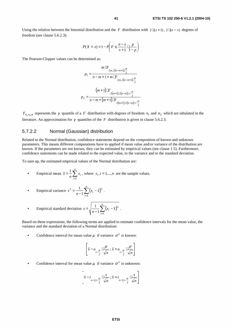
ETSI
ETSI TS 102 250-6 V1.2.1 (2004-10) 41
Using the relation between the binomial distribution and the F distribution with )(2,)1(2 xnx −⋅+⋅ degrees of
freedom (see clause 5.6.2.3):
−⋅
+−≤−=<
p
p
x
xnFPxXP
111)(
The Pearson-Clopper values can be determined as:
( )
( )2
;12,2
2;12,2
1 1 α
α
+−
+−
⋅++−
⋅
=mnm
mnm
Fmmn
Fm
p
( )( ) ( )
( )( ) ( )
21;2,12
21;2,12
2 1
1
α
α
−−+
−−+
⋅++−
⋅+
=mnm
mnm
Fmmn
Fm
p
γ;, 21 nnF represents the γ quantile of a F distribution with degrees of freedom 1n and 2n which are tabulated in the
literature. An approximation for γ quantiles of the F distribution is given in clause 5.6.2.3.
5.7.2.2 Normal (Gaussian) distribution
Related to the Normal distribution, confidence statements depend on the composition of known and unknown parameters. This means different computations have to applied if mean value and/or variance of the distribution are known. If the parameters are not known, they can be estimated by empirical values (see clause 1.5). Furthermore, confidence statements can be made related to the expected value, to the variance and to the standard deviation.
To sum up, the estimated empirical values of the Normal distribution are:
• Empirical mean ∑=
=n
iix
nx
1
1, where nixi ,...,1, = are the sample values.
• Empirical variance ( )∑=
−−
=n
ii xx
ns
1
22
1
1.
• Empirical standard deviation ( )∑=
−−
=n
ii xx
ns
1
2
1
1.
Based on these expressions, the following terms are applied to estimate confidence intervals for the mean value, the variance and the standard deviation of a Normal distribution:
• Confidence interval for mean value µ if variance 2σ is known:
⋅+⋅−
−− nux
nux
σσαα2
12
1;
• Confidence interval for mean value µ if variance 2σ is unknown:
⋅+⋅−
−−−− n
stx
n
stx
nn2
1;12
1;1; αα
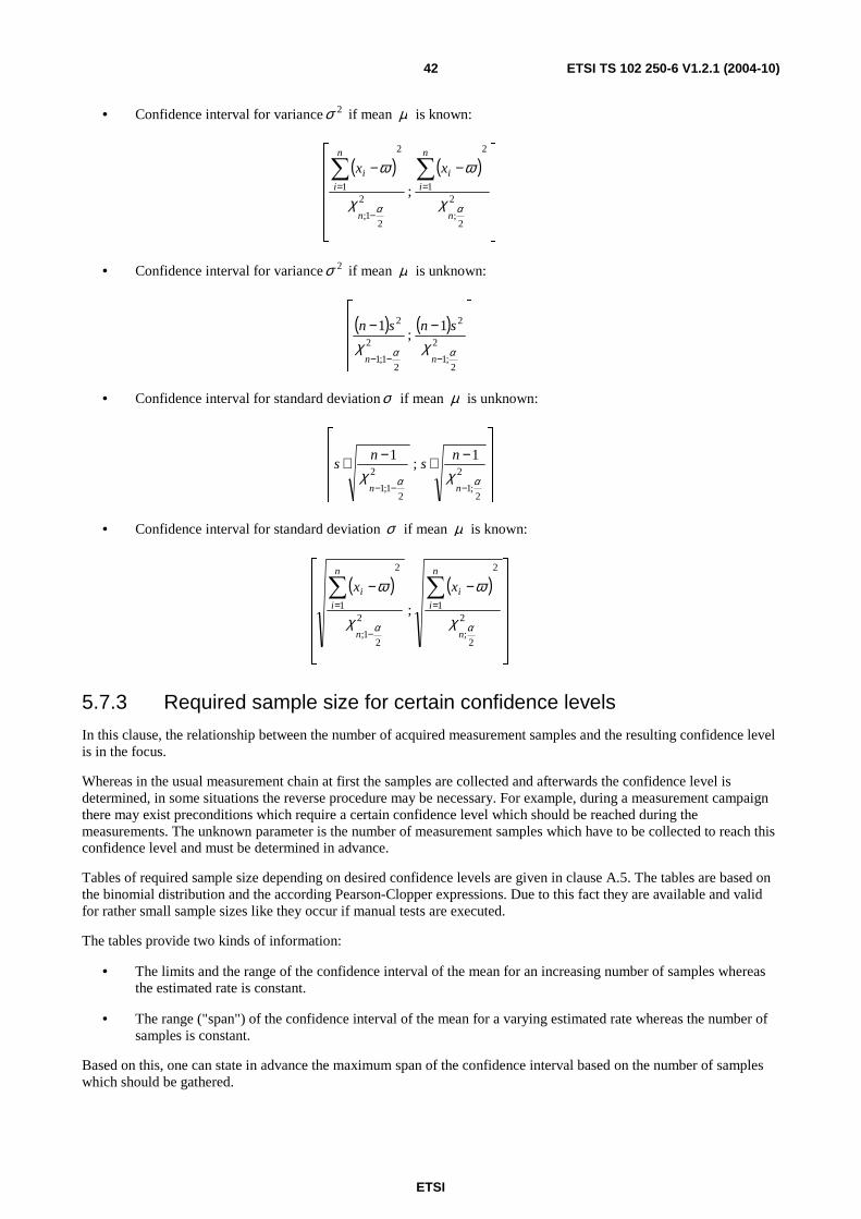
ETSI
ETSI TS 102 250-6 V1.2.1 (2004-10) 42
• Confidence interval for variance 2σ if mean µ is known:
( ) ( )
−− ∑∑
=
−
=2
2;
2
12
21;
2
1 ;αα χ
ϖ
χ
ϖ
n
n
ii
n
n
ii xx
• Confidence interval for variance 2σ if mean µ is unknown:
( ) ( )
−−
−−−
2
2;1
2
2
21;1
2 1;
1
αα χχnn
snsn
• Confidence interval for standard deviationσ if mean µ is unknown:
−⋅−⋅−−−
2
2;1
2
21;1
1;
1
αα χχnn
ns
ns
• Confidence interval for standard deviation σ if mean µ is known:
( ) ( )
−− ∑∑=
−
=2
2;
2
12
21;
2
1 ;αα χ
ϖ
χ
ϖ
n
n
ii
n
n
ii xx
5.7.3 Required sample size for certain confidence levels
In this clause, the relationship between the number of acquired measurement samples and the resulting confidence level is in the focus.
Whereas in the usual measurement chain at first the samples are collected and afterwards the confidence level is determined, in some situations the reverse procedure may be necessary. For example, during a measurement campaign there may exist preconditions which require a certain confidence level which should be reached during the measurements. The unknown parameter is the number of measurement samples which have to be collected to reach this confidence level and must be determined in advance.
Tables of required sample size depending on desired confidence levels are given in clause A.5. The tables are based on the binomial distribution and the according Pearson-Clopper expressions. Due to this fact they are available and valid for rather small sample sizes like they occur if manual tests are executed.
The tables provide two kinds of information:
• The limits and the range of the confidence interval of the mean for an increasing number of samples whereas the estimated rate is constant.
• The range ("span") of the confidence interval of the mean for a varying estimated rate whereas the number of samples is constant.
Based on this, one can state in advance the maximum span of the confidence interval based on the number of samples which should be gathered.
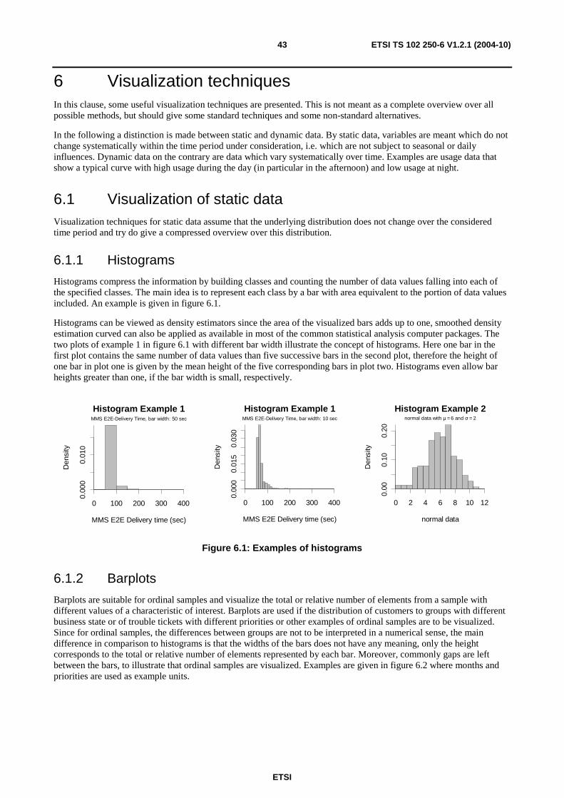
ETSI
ETSI TS 102 250-6 V1.2.1 (2004-10) 43
6 Visualization techniques In this clause, some useful visualization techniques are presented. This is not meant as a complete overview over all possible methods, but should give some standard techniques and some non-standard alternatives.
In the following a distinction is made between static and dynamic data. By static data, variables are meant which do not change systematically within the time period under consideration, i.e. which are not subject to seasonal or daily influences. Dynamic data on the contrary are data which vary systematically over time. Examples are usage data that show a typical curve with high usage during the day (in particular in the afternoon) and low usage at night.
6.1 Visualization of static data Visualization techniques for static data assume that the underlying distribution does not change over the considered time period and try do give a compressed overview over this distribution.
6.1.1 Histograms
Histograms compress the information by building classes and counting the number of data values falling into each of the specified classes. The main idea is to represent each class by a bar with area equivalent to the portion of data values included. An example is given in figure 6.1.
Histograms can be viewed as density estimators since the area of the visualized bars adds up to one, smoothed density estimation curved can also be applied as available in most of the common statistical analysis computer packages. The two plots of example 1 in figure 6.1 with different bar width illustrate the concept of histograms. Here one bar in the first plot contains the same number of data values than five successive bars in the second plot, therefore the height of one bar in plot one is given by the mean height of the five corresponding bars in plot two. Histograms even allow bar heights greater than one, if the bar width is small, respectively.
Histogram Example 1
MMS E2E Delivery time (sec)
Den
sity
0 100 200 300 400
0.00
00.
010
MMS E2E-Delivery Time, bar width: 50 sec
Histogram Example 1
MMS E2E Delivery time (sec)
Den
sity
0 100 200 300 400
0.00
00.
015
0.03
0
MMS E2E-Delivery Time, bar width: 10 sec
Histogram Example 2
normal data
Den
sity
0 2 4 6 8 10 12
0.00
0.10
0.20
normal data with µ = 6 and σ = 2
Figure 6.1: Examples of histograms
6.1.2 Barplots
Barplots are suitable for ordinal samples and visualize the total or relative number of elements from a sample with different values of a characteristic of interest. Barplots are used if the distribution of customers to groups with different business state or of trouble tickets with different priorities or other examples of ordinal samples are to be visualized. Since for ordinal samples, the differences between groups are not to be interpreted in a numerical sense, the main difference in comparison to histograms is that the widths of the bars does not have any meaning, only the height corresponds to the total or relative number of elements represented by each bar. Moreover, commonly gaps are left between the bars, to illustrate that ordinal samples are visualized. Examples are given in figure 6.2 where months and priorities are used as example units.
ETSI
ETSI TS 102 250-6 V1.2.1 (2004-10) 44
Barplot Example 1
Tro
uble
Tic
kets
050
100
150
Jan
Feb
Mrz
Apr
Mai
Jun
Jul
Aug
Trouble Tickets in a specific category
Barplot Example 1
Tro
uble
Tic
kets
050
100
150
Jan
Feb
Mrz
Apr
Mai
Jun
Jul
Aug
Trouble Tickets in a specific category
Source 1Source 2
Barplot Example 2
Tro
uble
Tic
kets
020
040
060
080
0
P 1 P 2 P 3 P 4
Trouble Tickets by Priority
Figure 6.2: Examples of barplots
6.1.3 QQ-Plots
An important tool for checking the normality assumption is the so called Quantile-Quantile-Plot or QQ-Plot. This plot compares the quantiles of two distributions in a scatter plot. In particular the theoretical quantiles of the normal distribution may be compared to empirical quantiles from a sample of interest, but also any other distributional assumptions can be checked, respectively.
In case of a normal QQ-Plot, theoretical quantiles can be taken from the standard normal distribution. The points of the resulting scatter plot should then fall on a straight line with slope corresponding to the empirical standard deviation of the sample. Figure 6.3 gives three example normal QQ-Plots for normal and non-normal samples.
In the first plot, the sample is in fact normal and the normal QQ-Plot also supports the assumption of normal data. For both other plots, non-normal data are simulated to visualize the normal QQ-Plot in cases where the assumptions are violated. In the second example, the entire distribution disagrees with the normal assumption while in example three, only the right tail of the distribution does not agree with the normality assumption.
-3 -2 -1 0 1 2 3
02
46
812
Normal QQ-Plot Example 1
Theoretical Quantiles
Sam
ple
Qua
ntile
s
Slope: σ̂ = 2.04
normal data with µ = 6 and σ = 2
-3 -2 -1 0 1 2 3
010
2030
Normal QQ-Plot Example 2
Theoretical Quantiles
Sam
ple
Qua
ntile
s
Slope: σ̂ = 5.25
exponential data with λ = 1 6
-3 -2 -1 0 1 2 3
05
1015
Normal QQ-Plot Example 3
Theoretical Quantiles
Sam
ple
Qua
ntile
s
Slope: σ̂ = 2.31
t-distributed data (10 df) × 2 +6
Figure 6.3: Examples of normal QQ-Plots
6.1.4 Boxplots
Boxplots, as the name suggests, consist of a box and some additional shapes called whiskers. These visualize the data information compressed in only a few numbers based on quantiles of the empirical distribution. The end-points of the box are given by the 25 % and 75 %-Quantile (also called Quartiles), the horizontal line is given by the median of the data (50 %-Quantile). Therefore the box contains 50 % of the given data. The whiskers (in the example plots represented by dotted lines) extend to the most extreme data point which is no more than 1,5 times the interquartile range (between the 25 %-Quantile and the 75 %-Quantile) from the box. All data points outside this interval are individually added and may be viewed as outliers. Figure 6.4 gives some boxplot examples.
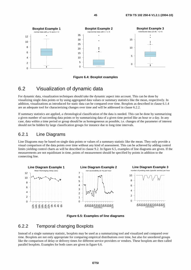
ETSI
ETSI TS 102 250-6 V1.2.1 (2004-10) 45
0
2
4
6
8
10
12
Boxplot Example 1normal data with µ = 6 and σ = 2
0
5
10
15
20
25
30
35
Boxplot Example 2exponential data with λ = 1 6
0
5
10
15
Boxplot Example 3t-distributed data (10 df) × 2 +6
Figure 6.4: Boxplot examples
6.2 Visualization of dynamic data For dynamic data, visualization techniques should take the dynamic aspect into account. This can be done by visualizing single data points or by using aggregated data values or summary statistics like the mean, respectively. In addition, visualizations as introduced for static data can be compared over time. Boxplots as described in clause 6.1.4 are an adequate tool for characterizing changes over time and will be addressed in clause 6.2.2.
If summary statistics are applied, a chronological classification of the data is needed. This can be done by summarizing a given number of succeeding data points or by summarizing data of a given time period like an hour or a day. In any case, data within a time period or group should be as homogeneous as possible, i.e. changes of the parameter of interest should not be hidden by large classification groups for instance due to long time intervals.
6.2.1 Line Diagrams
Line Diagrams may be based on single data points or values of a summary statistic like the mean. They only provide a visual comparison of the data points over time without any kind of assessment. This can be achieved by adding control limits yielding control charts as will be described in clause 9.2. In figure 6.5, examples of line diagrams are given. If the measurements are not equidistant in time, points of measurement should be specified by points in addition to the connecting line.
Line Diagram Example 1
12h
14h
16h
18h
20h
22h 0h 2h 4h 6h
0
2
4
6
8
10
12Mean Recharging Delay (sec)
Line Diagram Example 2
0
1
2
3
4
5
6
7
0h 3h 6h 9h 12h
15h
18h
21h 0h 3h 6h 9h 12h
non-accessibility (in %) per hour
Line Diagram Example 3
0
2
4
6
8
10
0h 3h 6h 9h 12h
15h
18h
21h 0h 3h 6h 9h 12h
number of probing trials (specific service) per hour
Figure 6.5: Examples of line diagrams
6.2.2 Temporal changing Boxplots
Instead of a single summary statistic, boxplots may be used as a summarizing tool and visualized and compared over time. Boxplots are not only appropriate for comparing empirical distributions over time, but also for unordered groups like the comparison of delay or delivery times for different service providers or vendors. These boxplots are then called parallel boxplots. Examples for both cases are given in figure 6.6.
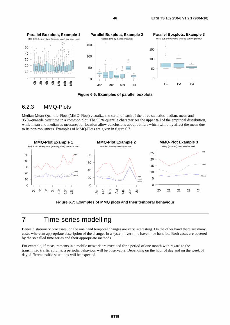
ETSI
ETSI TS 102 250-6 V1.2.1 (2004-10) 46
Parallel Boxplots, Example 1
0
10
20
30
40
50
0h 3h 6h 9h 12h
15h
18h
SMS E2E-Delivery time (probing trials) per hour (sec)
Parallel Boxplots, Example 2
0
50
100
150
Jan Mrz Mai Jul
reaction time by month (minutes)
Parallel Boxplots, Example 3
0
50
100
150
P1 P2 P3
MMS E2E Delivery time (sec) by service provider
Figure 6.6: Examples of parallel boxplots
6.2.3 MMQ-Plots
Median-Mean-Quantile-Plots (MMQ-Plots) visualize the serial of each of the three statistics median, mean and 95 %-quantile over time in a common plot. The 95 %-quantile characterizes the upper tail of the empirical distribution, while mean and median as measures for location allow conclusions about outliers which will only affect the mean due to its non-robustness. Examples of MMQ-Plots are given in figure 6.7.
MMQ-Plot Example 1
Q95
Median
Mean
0
10
20
30
40
50
0h 3h 6h 9h 12h
15h
18h
SMS E2E-Delivery time (probing trials) per hour (sec)
MMQ-Plot Example 2
Q95
MedianMean
0
20
40
60
80
Jan
Feb
Mrz
Apr
Mai
Jun
Jul
reaction time by month (minutes)
MMQ-Plot Example 3
Q95
Median
Mean
0
5
10
15
20
25
20 21 22 23 24
delay (minutes) per calendar week
Figure 6.7: Examples of MMQ plots and their temporal behaviour
7 Time series modelling Beneath stationary processes, on the one hand temporal changes are very interesting. On the other hand there are many cases where an appropriate description of the changes in a system over time have to be handled. Both cases are covered by the so called time series and their appropriate methods.
For example, if measurements in a mobile network are executed for a period of one month with regard to the transmitted traffic volume, a periodic behaviour will be observable. Depending on the hour of day and on the week of day, different traffic situations will be expected.
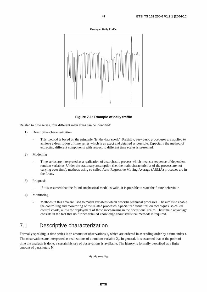
ETSI
ETSI TS 102 250-6 V1.2.1 (2004-10) 47
Example: Daily Traffic
Figure 7.1: Example of daily traffic
Related to time series, four different main areas can be identified:
1) Descriptive characterization
- This method is based on the principle "let the data speak". Partially, very basic procedures are applied to achieve a description of time series which is as exact and detailed as possible. Especially the method of extracting different components with respect to different time scales is presented.
2) Modelling
- Time series are interpreted as a realization of a stochastic process which means a sequence of dependent random variables. Under the stationary assumption (i.e. the main characteristics of the process are not varying over time), methods using so called Auto-Regressive Moving Average (ARMA) processes are in the focus.
3) Prognosis
- If it is assumed that the found stochastical model is valid, it is possible to state the future behaviour.
4) Monitoring
- Methods in this area are used to model variables which describe technical processes. The aim is to enable the controlling and monitoring of the related processes. Specialized visualization techniques, so called control charts, allow the deployment of these mechanisms in the operational realm. Their main advantage consists in the fact that no further detailed knowledge about statistical methods is required.
7.1 Descriptive characterization Formally speaking, a time series is an amount of observations xt which are ordered in ascending order by a time index t.
The observations are interpreted as realizations of a random variable Xt. In general, it is assumed that at the point of time the analysis is done, a certain history of observations is available. The history is formally described as a finite amount of parameters N.
Nxxx ,...,, 21
ETSI
ETSI TS 102 250-6 V1.2.1 (2004-10) 48
Talking in a more practical manner, the observations are represented by certain measurement results which are collected over time and which are analysed in their order of occurrence. Furthermore, the observations can be distinguished according to their timely occurrence: A stochastical process can be observed at fixed points of time which leads to equally spaced intervals between the observations. Another way to observe a process is by executing permanent measurements which deliver measurement results related to some events, so called event data. In effect, the time intervals between consecutive events may vary heavily. In this case it may be appropriate to approximate the situation at fixed points of time. This allows to use mechanisms which are designed for discrete time series.
7.1.1 Empirical moments
Similar to the handling of one-dimensional measurement results, descriptive characteristics (clause 5) can be deployed to describe the main characteristics of a time series. In particular, the arithmetic mean value or the variance respectively the standard deviation are addressed by this issue.
However, these global parameters of time series are only applicable if there is no systematic change in the series, so called stationary time series. In these cases, a movement in a certain direction (i.e. a trend) is not allowed. Concerning non-stationary time series it might be useful to fragment the series in smaller parts. Then, the partial time series can be assumed to be approximately stationary. This allows to use some procedures with a local meaning which are presented in clause 7.1.4.
Beyond this, the question arises if dependencies exist between different observations at different points of time. Corresponding to the covariance, the autocovariance function:
∑ −−= +t
jttj xxxxN
c ))((1
and the autocorrelation function:
0c
cr j
j =
are defined to measure linear dependencies between succeeding observations of a process. Both functions are defined as functions of the temporal difference (lags) j = - (N-1), .., -1, 0, 1, ..., (N-1) between the observations.
The graphical representation of the autocorrelation function rj is named correlogram. Correlograms are of high relevance for finding cyclic (i.e. periodic) structures in the gathered measurement data.
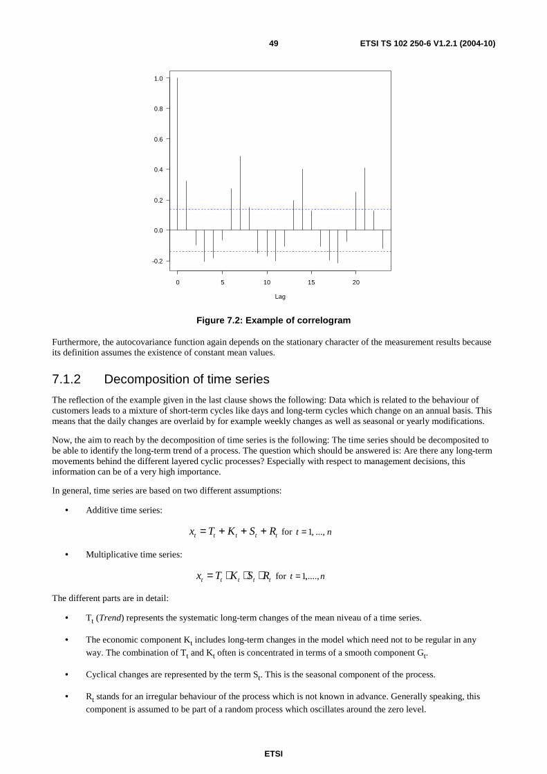
ETSI
ETSI TS 102 250-6 V1.2.1 (2004-10) 49
0 5 10 15 20
-0.2
0.0
0.2
0.4
0.6
0.8
1.0
Lag
Figure 7.2: Example of correlogram
Furthermore, the autocovariance function again depends on the stationary character of the measurement results because its definition assumes the existence of constant mean values.
7.1.2 Decomposition of time series
The reflection of the example given in the last clause shows the following: Data which is related to the behaviour of customers leads to a mixture of short-term cycles like days and long-term cycles which change on an annual basis. This means that the daily changes are overlaid by for example weekly changes as well as seasonal or yearly modifications.
Now, the aim to reach by the decomposition of time series is the following: The time series should be decomposited to be able to identify the long-term trend of a process. The question which should be answered is: Are there any long-term movements behind the different layered cyclic processes? Especially with respect to management decisions, this information can be of a very high importance.
In general, time series are based on two different assumptions:
• Additive time series:
ttttt RSKTx +++= for nt ...,,1=
• Multiplicative time series:
ttttt RSKTx ⋅⋅⋅= for nt ,....,1=
The different parts are in detail:
• Tt (Trend) represents the systematic long-term changes of the mean niveau of a time series.
• The economic component Kt includes long-term changes in the model which need not to be regular in any
way. The combination of Tt and Kt often is concentrated in terms of a smooth component Gt.
• Cyclical changes are represented by the term St. This is the seasonal component of the process.
• Rt stands for an irregular behaviour of the process which is not known in advance. Generally speaking, this
component is assumed to be part of a random process which oscillates around the zero level.
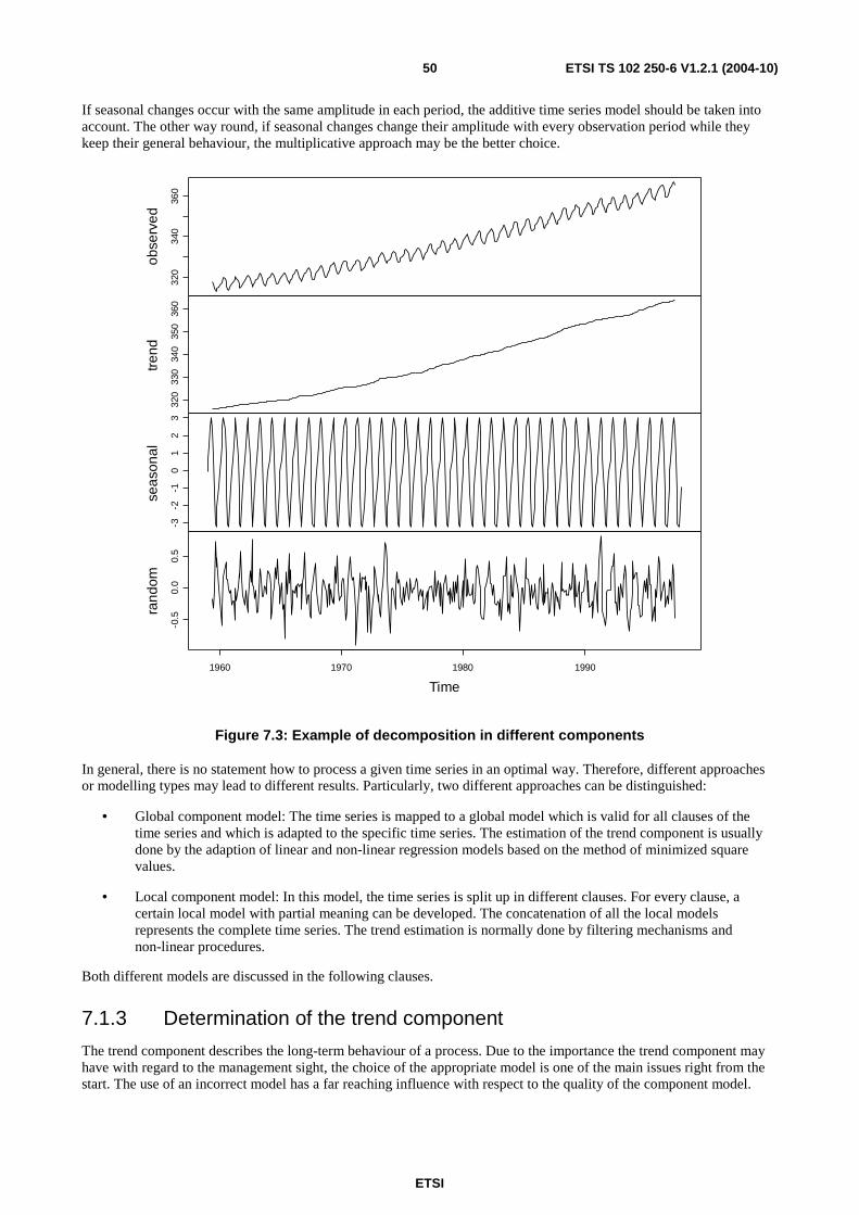
ETSI
ETSI TS 102 250-6 V1.2.1 (2004-10) 50
If seasonal changes occur with the same amplitude in each period, the additive time series model should be taken into account. The other way round, if seasonal changes change their amplitude with every observation period while they keep their general behaviour, the multiplicative approach may be the better choice.
320
340
360
obse
rved
320
330
340
350
360
trend
-3-2
-10
12
3
seas
onal
-0.5
0.0
0.5
rand
om
1960 1970 1980 1990
Time
Figure 7.3: Example of decomposition in different components
In general, there is no statement how to process a given time series in an optimal way. Therefore, different approaches or modelling types may lead to different results. Particularly, two different approaches can be distinguished:
• Global component model: The time series is mapped to a global model which is valid for all clauses of the time series and which is adapted to the specific time series. The estimation of the trend component is usually done by the adaption of linear and non-linear regression models based on the method of minimized square values.
• Local component model: In this model, the time series is split up in different clauses. For every clause, a certain local model with partial meaning can be developed. The concatenation of all the local models represents the complete time series. The trend estimation is normally done by filtering mechanisms and non-linear procedures.
Both different models are discussed in the following clauses.
7.1.3 Determination of the trend component
The trend component describes the long-term behaviour of a process. Due to the importance the trend component may have with regard to the management sight, the choice of the appropriate model is one of the main issues right from the start. The use of an incorrect model has a far reaching influence with respect to the quality of the component model.
ETSI
ETSI TS 102 250-6 V1.2.1 (2004-10) 51
Furthermore, wrong assumptions may lead to misinterpretations. For example, if a linear trend model is introduced, the conclusions drawn from such a model are restricted to a linear character. It is not possible to describe processes which own a more complex function which such a simple model. If it is done anyhow, the resulting conclusions may be completely wrong.
7.1.3.1 Trend function types
Different types of trend functions are possible. All of them introduce some unknown coefficients ai which must be
determined by calculation or estimation. The subsequent clauses introduce different approaches and their characteristics.
7.1.3.1.1 Linear trend function
The most well-known approach to model a trend function is a linear function. It is assumed that the observations xt
depend on the time index t in a linear manner. This relation can be formalized by the expression:
taaxt 21 +=
It is very easy to interpret this model since the sign of a1 represents if the time series increases (positive sign) or
decreases (negative sign) over time.
7.1.3.1.2 Polynomial trend function
Extending the linear approach, the polynomial approach assumes that a time series can be described as the composition of different functions m:
)()()( 2211 tmatmatmax kkt +++= K
mi(t) are arbitrary known functions. It is important that the combination of all the single expressions aimi(t) is linear.
A very simple approach is to define the mi functions as polynomials of rank (i-1). Then, the approach reads:
121
−+++= kkt tataax K
According to the theory, p + 1 points of a function can be perfectly approximated if a polynomial of rank p is used. This means it is possible to reach a perfect approximation between model and any time series in any case. However, there are two serious disadvantages:
• Resulting models are very complex and cannot be interpreted in a simple manner (compared with the basic trend model).
• The assimilation takes only the available data into account. Therefore, it is not possible to make statements about the behaviour in the future.
Both effects are considered as overfitting effects.
ETSI
ETSI TS 102 250-6 V1.2.1 (2004-10) 52
7.1.3.1.3 Non-linear trend models
Lots of different non-linear trend models are available. Because of difficulties to describe all models in a general manner, this clause concentrates on some important cases with a very special meaning:
1) Exponential models:
)()()( 2211 tmatmatmat
kkex +++= K
2) Power models:
kak
aat tmtmtmx )()()( 2
211
K⋅⋅=
Both models can be reduced to linear models if a logarithmic operation is applied. Then, the multiplication respective exponentiation is reduced to a simple addition.
3) Logistic models.
In many use cases, it can be assumed that natural limits exist which can be reached by a time series if observations are done over a longer period of time. For example, the growth of customers in a network follows a function which is shaped like an S. In other words, these processes are constrained by saturation effects.
Formally, these time series can be described the following approach:
tat
ea
ax
32
1−+
=
In this case the values of the time series converge to the saturation at the value G = a1/a2.
7.1.3.2 Trend estimation
The common principle behind the different presented approaches is to determine the unknown parameters ai. Regularly,
this is done by estimating the minimization of a squared expression based on a difference. The difference is built by comparing the measurement value xt with the according approximation given by the chosen approach. Afterwards, the
resulting difference is squared and summed up. For the polynomial approach, the according overall expression reads:
( ) Minimum)()()(
2
12211 →+++−=∑
=
N
ikkt tmatmatmaxQ K
Now, the task is to minimize the expression for Q.
To solve the minimization problem, partial derivatives are calculated. In detail, Q is derived with respect to each of the parameters ai:
nia
Q
i
,,1,0!
K==∂∂
A system of so called normal equations is the result of this calculation. Under the assumption of linear independency of the different functions mi, a closed solution exists so that the different parameters ai can be identified.
Related to non-linear models, the minimization approach leads to normal equations that cannot be solved explicitly. A further leading approach which might solve these problems is based on linear approximations and is called the Gauss-Newton procedure. Additional information can be found in [BAT] (see bibliography).
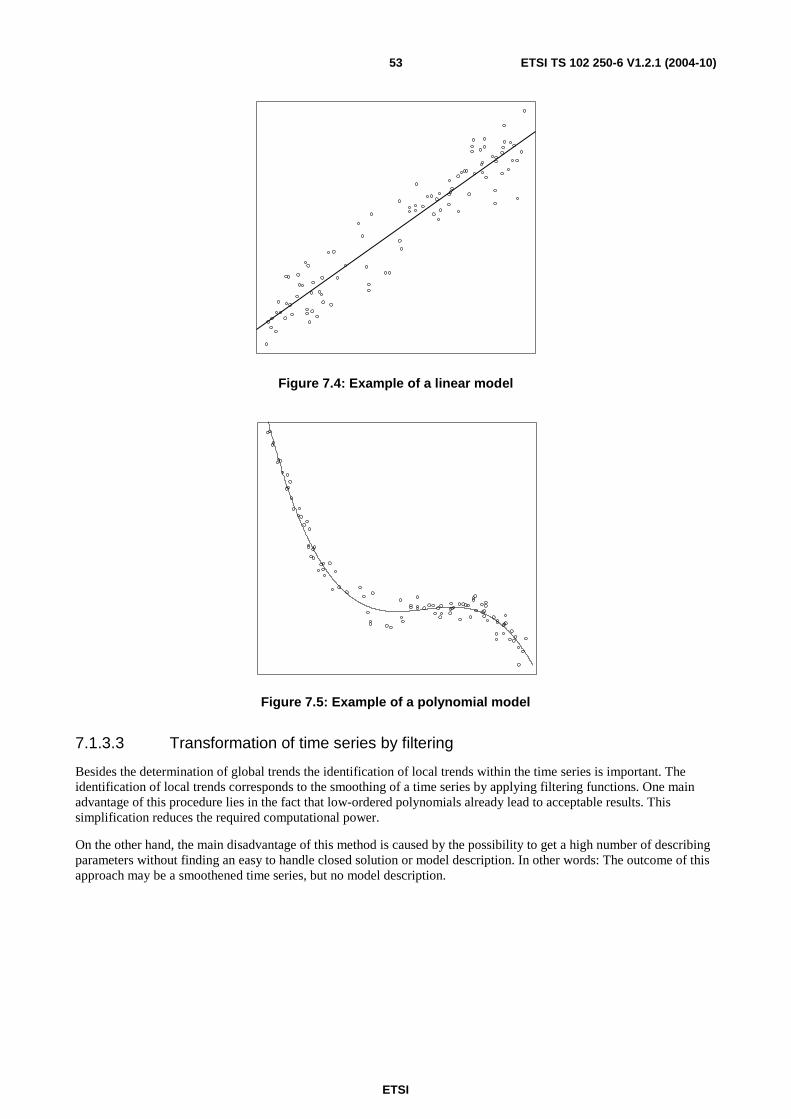
ETSI
ETSI TS 102 250-6 V1.2.1 (2004-10) 53
Figure 7.4: Example of a linear model
Figure 7.5: Example of a polynomial model
7.1.3.3 Transformation of time series by filtering
Besides the determination of global trends the identification of local trends within the time series is important. The identification of local trends corresponds to the smoothing of a time series by applying filtering functions. One main advantage of this procedure lies in the fact that low-ordered polynomials already lead to acceptable results. This simplification reduces the required computational power.
On the other hand, the main disadvantage of this method is caused by the possibility to get a high number of describing parameters without finding an easy to handle closed solution or model description. In other words: The outcome of this approach may be a smoothened time series, but no model description.
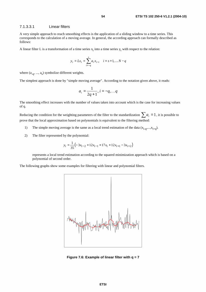
ETSI
ETSI TS 102 250-6 V1.2.1 (2004-10) 54
7.1.3.3.1 Linear filters
A very simple approach to reach smoothing effects is the application of a sliding window to a time series. This corresponds to the calculation of a moving average. In general, the according approach can formally described as follows:
A linear filter L is a transformation of a time series xt into a time series yt with respect to the relation:
qNsixaLxys
qiititt −+=== ∑
−=− K,1
where (a-q, ..., as) symbolize different weights.
The simplest approach is done by "simple moving average". According to the notation given above, it reads:
qqiq
ai K,,12
1 −=+
=
The smoothing effect increases with the number of values taken into account which is the case for increasing values of q.
Reducing the condition for the weighting parameters of the filter to the standardization ∑ =1ia , it is possible to
prove that the local approximation based on polynomials is equivalent to the filtering method:
1) The simple moving average is the same as a local trend estimation of the data (xi-q,...,xi+q).
2) The filter represented by the polynomial:
( )2112 3121712335
1++−− −+++−= tttttt xxxxxy
represents a local trend estimation according to the squared minimization approach which is based on a polynomial of second order.
The following graphs show some examples for filtering with linear and polynomial filters.
Figure 7.6: Example of linear filter with q = 7
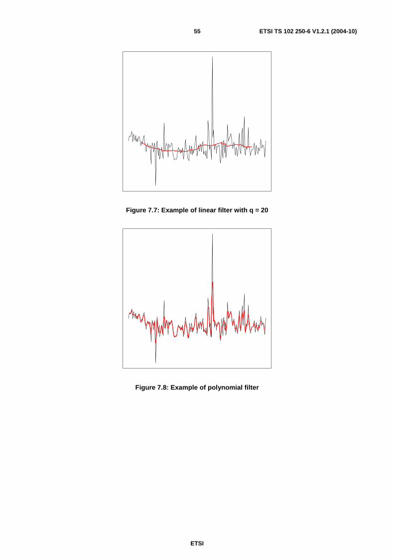
ETSI
ETSI TS 102 250-6 V1.2.1 (2004-10) 55
Figure 7.7: Example of linear filter with q = 20
Figure 7.8: Example of polynomial filter
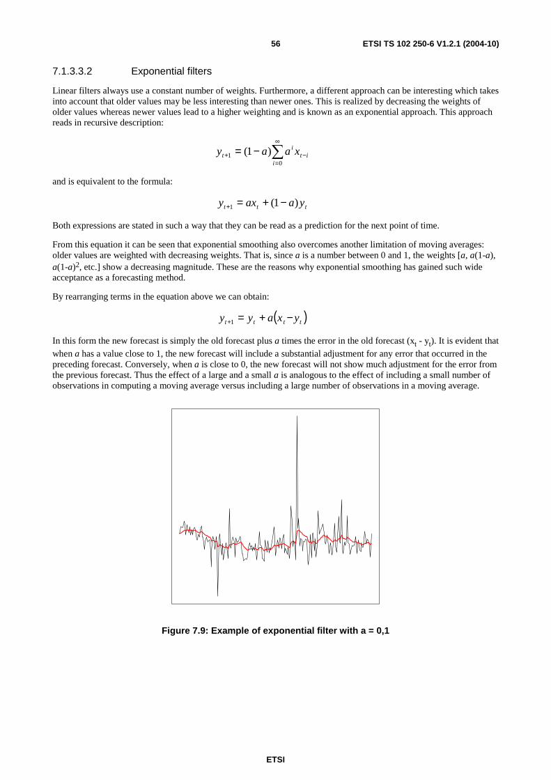
ETSI
ETSI TS 102 250-6 V1.2.1 (2004-10) 56
7.1.3.3.2 Exponential filters
Linear filters always use a constant number of weights. Furthermore, a different approach can be interesting which takes into account that older values may be less interesting than newer ones. This is realized by decreasing the weights of older values whereas newer values lead to a higher weighting and is known as an exponential approach. This approach reads in recursive description:
∑∞
=−+ −=
01 )1(
iit
it xaay
and is equivalent to the formula:
ttt yaaxy )1(1 −+=+
Both expressions are stated in such a way that they can be read as a prediction for the next point of time.
From this equation it can be seen that exponential smoothing also overcomes another limitation of moving averages: older values are weighted with decreasing weights. That is, since a is a number between 0 and 1, the weights [a, a(1-a), a(1-a)2, etc.] show a decreasing magnitude. These are the reasons why exponential smoothing has gained such wide acceptance as a forecasting method.
By rearranging terms in the equation above we can obtain:
( )tttt yxayy −+=+1
In this form the new forecast is simply the old forecast plus a times the error in the old forecast (xt - yt). It is evident that when a has a value close to 1, the new forecast will include a substantial adjustment for any error that occurred in the preceding forecast. Conversely, when a is close to 0, the new forecast will not show much adjustment for the error from the previous forecast. Thus the effect of a large and a small a is analogous to the effect of including a small number of observations in computing a moving average versus including a large number of observations in a moving average.
Figure 7.9: Example of exponential filter with a = 0,1
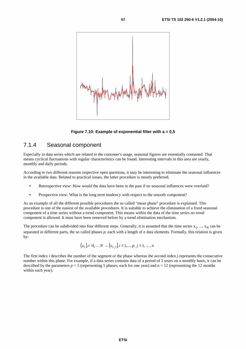
ETSI
ETSI TS 102 250-6 V1.2.1 (2004-10) 57
Figure 7.10: Example of exponential filter with a = 0,5
7.1.4 Seasonal component
Especially in data series which are related to the customer's usage, seasonal figures are essentially contained. That means cyclical fluctuations with regular characteristics can be found. Interesting intervals in this area are yearly, monthly and daily periods.
According to two different reasons respective open questions, it may be interesting to eliminate the seasonal influences in the available data. Related to practical issues, the latter procedure is mostly preferred.
• Retrospective view: How would the data have been in the past if no seasonal influences were overlaid?
• Prospective view: What is the long term tendency with respect to the smooth component?
As an example of all the different possible procedures the so called "mean phase" procedure is explained. This procedure is one of the easiest of the available procedures. It is suitable to achieve the elimination of a fixed seasonal component of a time series without a trend component. This means within the data of the time series no trend component is allowed. It must have been removed before by a trend elimination mechanism.
The procedure can be subdivided into four different steps. Generally, it is assumed that the time series x1, ..., xN can be separated in different parts, the so called phases p, each with a length of n data elements. Formally, this relation is given by:
( ) ( ) njpixNtx jit ,,1,,1, ,1, , KKK ==→=
The first index i describes the number of the segment or the phase whereas the second index j represents the consecutive number within this phase. For example, if a data series contains data of a period of 5 years on a monthly basis, it can be described by the parameters p = 5 (representing 5 phases, each for one year) and n = 12 (representing the 12 months within each year).
ETSI
ETSI TS 102 250-6 V1.2.1 (2004-10) 58
The following calculations implement the already mentioned four steps to achieve data without underlying seasonal impacts:
1) Calculation of the average of different phases:
∑=
=p
ijij x
px
1,
1
2) Calculation of the total average:
∑=
=n
jjxx
1
3) Calculation of seasonal indices (seasonal factors):
x
xs j
j =
Related to the last mentioned calculation, the averaged phases jx are set into relation to the total average x . In the
example, the average of January is for example divided by the total average. This step is done for all of the different monthly averages. If January data is much above average, then si > 1. According to this, if January data is much below
average, si < 1 will be the result.
4) Calculation of seasonally adjusted values:
njpis
xy
j
jiji KK ,1,,1,,
, ===
This step concludes the basic calculation scheme related to the determination of the seasonal component.
8 Data aggregation Depending on the objective, i.e. for monitoring or reporting purposes, different types of aggregation may be of interest. Firstly, different granularities in time and space may be needed. Secondly, weighting of data may be considered for instance to generate the QoS perceived by the customer. This may be more or less straightforward, if the smallest time granularity is evenly spaced and the full information at any time point or interval is available, i.e. there are no missing data. However, data aggregation becomes more challenging if event data are considered, like data from active probing systems, or if data are missing and substitution algorithms are needed for defining meaningful results at higher aggregation levels.
In the following, after presenting some basic aggregation operators, different data sources and corresponding structures are distinguished, temporal and spatial aggregation levels are defined and estimation methods for incomplete data are suggested. Based on a summary of desirable attributes of aggregation procedures, an aggregation strategy is suggested and discussed. Subsequently, weighted aggregations are motivated and weighting methods are introduced.
8.1 Basic data aggregation operators Most common data aggregation operators are sums and means. Sums are applied if the total number of events, usage, etc. within a given time period is of interest, while means are commonly applied if some kind of averaging is needed. However, in particular for data out of time-interval measurements, means may not lead to interpretable and convincing aggregation results, therefore other summarizing statistics like the minimum, maximum, median and other quantiles of data are also used as aggregation operators. For quality of services measures like accessibilities, retainabilities and so on, ratios in the sense of fractions are used.
ETSI
ETSI TS 102 250-6 V1.2.1 (2004-10) 59
The combination of aggregation operators in a row might raise problems, even if the same operator is used at each single step. If the data basis is complete, the combination of sums on different aggregation levels, that is summing sums of lower levels for a higher level aggregation result, ensures a meaningful interpretation. If the considered time intervals are equidistant in addition, the same holds true for the combination of means on different aggregation levels. Minimum and maximum operators are also examples where this kind of combination is possible and meaningful. However, for other quantiles like the median or Q95, it is not recommended to base aggregations on higher levels on the results of lower aggregation levels, since for instance the median of subgroup-medians is not guaranteed to be near the overall median. Aggregation methods for fractions will be discussed later.
If different aggregation operators are combined one after another, the resulting values should be interpreted with great care. For instance the minimum and maximum of mean values from lower aggregation levels should not be mistaken as the range of the original data values. However, one can think of many examples where this kind of combination yields meaningful results that are of interest, for instance if different BSCs are compared with regard to QoS parameters, the median or quantiles of the values for all BSCs may be used as cut-points to identify BSCs performing particularly good or bad.
8.2 Data sources, structures and properties In the following, a distinction between raw data that may result from data sources with different attributes and parameters that are defined based on these raw data is made.
8.2.1 Raw data
For measuring QoS, data from a number of different data sources are used. These "raw data" are based on different measurement systems with possibly different granularities, differences due to release changes of the underlying systems and so on. Therefore raw data often come with a number of attributes that need to be taken into account for aggregation. Here performance data and event data are considered, although other data sources and types could also provide valuable information about QoS (like fault management data).
In the situation that not all data are available - which is a common problem not only in mobile communications - raw data are rarely substituted or adjusted, but are stored with the full source information to allow suitable parameter definition and estimation. This is often only possible by applying all available reference knowledge, for instance which or how many cells were supposed to deliver data for a given time period.
8.2.1.1 Performance data
Most performance data are given by Network Element (NE) counters. Due to different underlying systems or releases, these may be available in different temporal granularities, like values for 15 minutes from one system and values for hours from another system, respectively. Here basic operations are needed to enable a common data format in order to ensure that values are comparable and basic aggregations are needed for total NE counter values independent of underlying systems. In addition to results of basic aggregations, the total number of aggregated values or even additional detailed reference information needs to be stored.
Examples for performance data are the number of calls per hour per cell, the total number of call minutes per quarter-hour per cell or the number of started WAP-sessions per hour per cell.
8.2.1.2 Event data
Billing data are one example of event data that may provide information about the QoS. On the other hand, results from active probing systems are also in general not equally spaced over time. This may be due to varying duration of trials, possibly depending on network performance or other influences. Also there may be reasons to do a larger number of tests regarding a specific service over a given period of time, for instance if new services are launched.
Event data do not provide information of a time interval, but just a number of results, each for a corresponding point in time. To allow statements about time periods, it is either possible to use all original data points for defining and aggregating parameters for each time interval of interest, or as an alternative, relatively small time intervals have to be defined for which a first, "basic", aggregation step is carried out which then allows higher aggregations independent of the original data.
ETSI
ETSI TS 102 250-6 V1.2.1 (2004-10) 60
8.2.2 Key Performance Indicators / Parameters
A particular feature of a Key Performance Indicator (KPI or parameter) - in comparison to raw data - is given by the fact that KPIs are defined in an abstract manner, thereby allowing a common interpretation for parameters computed from different data sources and on various aggregation levels. Usually, there are two possible reasons for a parameter to be identified as a KPI, either:
• the KPI is a function aggregation of different parameters; or
• the KPI represents a very important quality measure related to the customer's perspective.
In the latter case, data aggregation is not necessarily implied.
Parameters are defined to serve specific purposes like answering questions about QoS or performance by utilizing raw data or basic aggregations of raw data. This might also include combinations of different data by mathematical operations like ratios. Unlike raw data, parameters are independent of the underlying software releases or system vendors. One could also define them as being independent of different underlying systems, if appropriate.
Parameters based on performance data are for instance the Cut-of-Call Ratio, which is based on two different NE counters, namely the number of unintentionally terminated calls divided by the number of successful call attempts times 100 %. Data from active probing systems allow the definition of parameters like the Recharging-Failure-Ratio, SMS-E2E-Failure-Ratios and so on.
For the definition and computation of parameters, rules for handling missing data are needed. Therefore methods for data substitution become a major point when talking about parameter computation and aggregation and will be covered in some detail after defining aggregation hierarchies of interest.
8.3 Aggregation hierarchies Aggregation hierarchies are commonly divided into temporal and spatial aggregation hierarchies, where temporal in fact refers to different time intervals while the term spatial may also cover aggregations over items with similar properties with respect to an attribute of interest.
8.3.1 Temporal aggregation
Temporal aggregation levels that should be used for a given parameter will depend on the intended use of the parameter as well as on the raw data frequency. For most parameters, sensible aggregations levels will be some or all of the ones given in the following set:
• quarter-hour;
• hour;
• day;
• week;
• month;
• quarter year;
• calendar year; and
• business year.
In addition, incomplete temporal aggregation levels can be defined, for instance cumulative values for the current week based on the daily values that are available so far. This is of particular interest for parameters that are based on ratios or mean values because these may be interpreted directly. For the interpretation of incomplete parameters that are based on sums, the number of covered time units has to be taken into account.
ETSI
ETSI TS 102 250-6 V1.2.1 (2004-10) 61
8.3.2 Spatial aggregation
Spatial aggregation originally refers to aggregation levels from the smallest possible units like radio cells (or even sectors) in mobile communications up to the entire network. This can be done from a technical point of view for instance by taking the order "cell - BSC - MSC - (branch) - entire network", or from a regional point of view by "cell - state / region - entire network".
As mentioned before, the term "spatial" may also be used in the context of summarizing cells with similar properties regarding an attribute of interest, like all cells that cover motorways, or the position of a cell in terms of the surrounding area, whether it belongs to a large city, a small town or a rural area. In these cases, spatially incoherent units are aggregated.
8.4 Parameter estimation methods The ideal situation of full information is rarely met in practice. Network elements or branches failing to deliver data in time are common reasons for missing data. Since in most situations, missing values as parameter values are unacceptable, even if parts of the raw data are missing, data estimation methods are needed. Depending on the situation, projection, substitution or combined estimation methods are suitable.
8.4.1 Projection method
The easiest method of data substitution is to project the available data to the entire time interval of interest. For example, if a fraction of 90 % of the expected data measuring the quality of a specific service within one hour is available and an hour-value is sought, these 90 % of the data are viewed as being representative for the hour of interest. If the aggregation contained of cumulating the entries, the value achieved by the available data has to be multiplied by a factor 100/90. If aggregated values are mean (or median) values, the mean (or median) of the available data is used as an aggregated value. If minimum or maximum values (or other quantiles besides the median) are sought as aggregated values, more sophisticated estimation methods should be applied like maximum likelihood methods.
Provided that a high percentage of data is available and there are no systematic reasons for missing data, the above procedure is sufficiently reasonable. However, an analysis of the times and circumstances of missing data might be of interest to identify the reasons, if missing values are becoming more frequent or appear suspect that there might be an underlying pattern.
If only a low percentage of data is available for a time period of interest, for instance less than 50 %, the above projection procedure is more than questionable. In particular if the parameter of interest is subject to dynamic changes over time, the results may be heavily biased. As an example consider usage data where a high percentage of missing data consists of records that should have been taken at night. If the usage is then estimated by projecting the available results, the usage is extremely overestimated. Therefore it seems sensible to define a "critical percentage" of data that need to be available for applying the method above. This percentage should depend on the specific service which is evaluated and on the needed precision of the aggregation results.
8.4.2 Substitution method
If the estimation of parameters can or should not be based on the available data, since a large number of data is missing or the data are not credible for some reason, substitution methods apply values from former time periods. This can either be done by using the last available value for the parameter of interest, which is only sensible for static parameters that are not subject to dynamic changes over time, or by using the last available value of a comparable time period with similar properties like the same day-type (weekday/Saturday/holiday or Sunday) or the same day of the week and the same time.

ETSI
ETSI TS 102 250-6 V1.2.1 (2004-10) 62
8.4.3 Application of estimation methods
Common problems that complicate the application of the methods suggested above are given by:
1) Unavailability of reference data: The number of missing data is needed for deciding which method should be used and for the application of the projection method.
2) Determination of values for substitution: Comparable time intervals have to be defined and substitution values may be stored in a data base, which needs to be updated and maintained. In addition, calendar information about holidays/working days, weekdays and so on is needed.
3) Parameters that are defined as ratios: Either numerator and denominator are estimated separately based on the available information for each part, or the ratio is estimated as a whole by using only data with information about both, numerator and denominator. In the situation of full information, there is no difference between both possibilities, in case some data are available for one part of the ratio and not for the other, both strategies yield different results.
Referring to data aggregation, the question arises, at which aggregation level an estimation should take place. Is it acceptable to use estimated values as a basis for higher aggregations? Data aggregation procedures combining both introduced methods are derived in the following, originating from a summary of desirable attributes of aggregation procedures.
8.4.4 Attributes of aggregation operators
Aggregation methods may be evaluated according to the following attributes:
1) The result should be meaningful, that is as near as possible to the true value of interest. In particular, NULL-values are not sensible as a result of a higher level aggregation. In addition, all information about missing values should be used to take non-available data into account, to avoid biased parameter values. (Moreover, the variance of parameter values caused by estimation methods should be as small as possible.)
2) Aggregation results should be reproducible and understandable. In particular, at higher aggregation levels no estimation procedure should be used so that results on a higher aggregation level are in accordance with values of the underlying level.
3) Aggregation results should not depend on the used aggregation paths, i.e. there should be no difference of results, if spatial or temporal aggregation steps are interchanged as well as direct aggregation and aggregation with intermediate steps should not lead to different results. Independence of paths refers to aggregation calculations.
4) Results should be consistent. On a given aggregation level, individual aggregation results should agree with total result, i.e. the sums for different branches should add up to the total sum for the company and so on. Consistency refers to aggregation results.
5) The applied calculation procedures should be rather easy. This also implies independence of past values like those from previous time periods.
6) Independence of network references like assignment of results to network elements.
In general, it is not possible to meet all requirements at the same time. Easy methods may lead to non-sensible results, while methods that contain estimation procedures often rely on values from previous time periods or network references and may be more sophisticated. In particular the requirements 1 and 5/6 are contradicting as estimation methods ignoring network references and past values will presumably often lead to worse results compared to methods that take into account all available information.
One idea to combine the above requirements to a certain extent is to define a smallest temporal and spatial aggregation level for which the data are completed by estimation procedures (for missing parameter data) or basic aggregations (for event data and parameter data with different lowest levels), like per hour per cell. This yields an equally spaced "complete" data pool and therefore simplifies all further aggregation steps and in particular ensures consistency of results and independence of aggregation paths.
ETSI
ETSI TS 102 250-6 V1.2.1 (2004-10) 63
One major disadvantage of this method is the fact that estimation procedures have to be applied on low aggregation levels which rely heavily on reference data and good substitution values or projection procedures. For parameters that are dynamic over time, time series methods as covered in clause 7 should be considered, which then implies more complicated calculation procedures for low aggregation levels and therefore might take some computation time.
8.5 Weighted aggregation In many situations, in particular if the QoS perceived by the customer is of interest, simple aggregations of the available information or estimated values are not very meaningful. A better approach would be to take into account e.g. how many users are affected if a service fails. That leads to the idea of weighted aggregation, where for instance the usage can be applied for weighting, respectively. It should be noted, however, that weighted aggregation methods will in general lead to non-consistent results in the sense of property 4 from clause 8.4.4.
8.5.1 Perceived QoS
Depending on the point of view and the corresponding intention of a parameter of interest, it appears reasonable to only consider users view instead of the network view e.g. by taking the usage of a service into account. Depending on the applied aggregation procedure, this may have already been done implicitly. For instance, if the aggregated cut-of-call-ratio for a particular week is considered, different aggregation procedures imply different weightings (it is assumed that values are available hourly):
1) If the cut-of-call-ratio is stored for hourly intervals and the weekly aggregation is done by averaging all values for the week of interest, no weighting is carried out and each hour viewed as being equally important. This does not correspond with the users perspective. (Note that a geometric rather than an arithmetic mean should be applied for averaging ratios.)
2) If the numerator and denominator are stored for hourly intervals and the weekly aggregation is done by first summing all entries for the numerator and denominator separately and then dividing both numbers, an implicit weighting is carried out. Since high usage time intervals contribute a larger number of call attempts than low usage intervals, thereby the users perspective is expressed.
When applying the first method, one should consider using weighted means instead of simple means. Depending on the type of parameter, weighted arithmetic means are computed according to:
∑=
=n
iiiw wxx
1
where 11
=∑=
n
iiw , weighted geometric means are given by:
( ) niiw wxx /1~ ∏=
where 1=∏ iw . (For unweighted arithmetic or geometric means, all weights are given by wi ≡ 1/n or wi ≡ 1,
respectively.)
Weights can either be based on true or average usage curves, but also on strategic reasons or any other procedure in accordance with the aim of the analysis. An average usage curve may for instance be achieved by averaging over the past 30 working days, the past 5 Saturdays and the past 5 Sundays or holidays or by applying some kind of time series modelling and forecasting methods. Weights based on usage curves are then computed as:
ii
i
uw
u=∑
or ii
i
uw
u=
∏
respectively, where ui is the true or estimated usage within time period i.
ETSI
ETSI TS 102 250-6 V1.2.1 (2004-10) 64
If the second method from above is applied, weighting is done implicitly with the actual usage curve. However, other problems arise in particular regarding missing data handling as mentioned in clause 8.4.3. For each time period, the percentage of missing data might be of interest for applying projection or substitution methods and to ensure that the cut-of-call-ratio does not exceed 1, e.g. the number of unintentionally terminated calls should not exceed the number of successful call attempts, one might only want to consider data pairs where both numbers are known. When using the first method, this could be avoided by estimating only on an hourly basis.
Remark: For ratios, higher level aggregations are commonly achieved by applying the second method because of the implicit weighting, which is more intuitive.
Data from active probing systems are generally not weighted implicitly, since probing frequencies are commonly non-representative for customer behaviour. In this context, the idea of weighting might even be of importance in more than one respect.
1) Since data from active probing systems are not equally spaced, a weighting of each trial result by the time between two trials in some way could be considered. This can either be realized by defining (rather small) time intervals for which all trials done within this interval are summarized without weighting or alternatively by computing using half of the time interval between the last trial and the current one and half of the time interval between the current trial and the next one as a basis for weighting. If such weighting is considered, an upper bound for the defined underlying intervals should be considered and strategies for the situation that the active probing system does not work or data are not delivered for a longer time period are to be thought of (estimation or NULL-values, depending on the situation and parameters of interest).
2) A second - and probably more important - way of weighting results from active probing system is the usage weighting for achieving the perceived QoS as explained before.
If both types of weighting are applied, combined weights are computed as ( )
( )i
ii
u tw
u t=∑
, where u(ti) is the usage
within time period ti assigned to probing trial i according to the distribution of trials over time (1st weighting), either for a basic aggregation level for further aggregation or for the desired aggregation level directly.
8.5.2 Weighted quantiles
For duration values as results from active probing trials, quantiles represent meaningful aggregation results on higher aggregation levels. From the above weighting discussion the necessity of determining weighted quantiles arises. Due to the calculation of quantiles based on ordered data values, a weighting similar to those for mean values is not applicable. Instead, a replication algorithm could be used for computing weighted quantiles. This algorithm simply repeats each value according to an assigned weight and calculates the desired quantile of the resulting new data set. (If weights are irrational, sensible rounding is needed.)
EXAMPLE: The original (ordered) data set of 10 MMS-E2E delivery times is given by 51, 55, 60, 61, 65, 70, 71, 72, 72, 80 seconds. These measurements have been taken at different daytimes and therefore get a weight of 1, if taken at night, 2, if taken in the morning or late in the evening and 4, if taken between noon and 8 p.m. for instance. According weights are therefore given by 1, 4, 2, 2, 1, 4, 4, 2, 1, 4 resulting in a data set with 25 data: 51, 55, 55, 55, 55, 60, 60, 61, 61, 65, 70, 70, 70, 70, 71, 71, 71, 71, 72, 72, 72, 80, 80, 80, 80. Quantiles from the original and the replicated data set will in general lead to slightly different results.
If a weighting according to some kind of usage curve is aimed, this curve can be used as a replication function or replication curve and represent the basis for defining the needed weights. To simplify the computation, weights may be defined by identifying the minimum of the replication function rmin and to define the weights according to:
=
min r
rroundw ii .
If a uniform concept for weighting of any kind of parameter is sought, the approach based on replication functions might also be used for means or non-accessibilities or other parameters of interest. Differences for instance between conventionally weighted means and means weighted by replication curves are only due to the applied rounding step for the latter approach.
ETSI
ETSI TS 102 250-6 V1.2.1 (2004-10) 65
8.6 Additional data aggregation operators In the following, some additional data aggregation operators are covered, adding to those mentioned in clause 8.1, that are in some sense individual regarding their attributes and/or application.
8.6.1 MAWD and BH
In particular for network maintenance an aggregation operator of interest is the "Monthly Average Working Day" (MAWD). This operator can be viewed as being an aggregation result as well as a possible weighting function for other aggregation operators.
The monthly average working day of a given data set is computed by filtering all data from working days within a given month first and then computing the mean value for each hour of the day over all data from corresponding hours. The result is therefore given by a vector of 24 entries, each corresponding to one hour of the day (0 h - 1 h, ..., 23 h - 24 h).
Based on the MAWD, the "Busy Hour" (BH) is defined as the hour in which the MAWD-vector takes its maximum value. In mathematical notation, this is argmax(m), where m = (m1, ..., m24)T is the vector resulting from applying the
MAWD operator.
8.6.2 AVGn
The class of parameters AVGn is applied for similar reasons as the BH-operator mentioned in clause 8.6.1. Both try to identify peaks of high usage or traffic, where the BH-operator considers hours where the highest usage is observed on average, while the AVGn-operators are interested in the maximum usage or traffic for a given calendar week. The mean of the n largest values realized on n different days (n between 1 and 5 or 7, depending on intended use) is defined as AVGn.
9 Assessment of performance indices
9.1 Estimation of performance parameters based on active service probing systems
End-to-end service probing systems yield valuable information about services and systems that may not be provided by the network elements alone. Active probing systems are used to view the customer perspective of the Quality of Service, i.e. the perceived QoS. Typical parameters that may be computed based on active probing systems are failure ratios, accessibilities and end-to-end-delivery times for a number of different services.
One characteristic of active probing systems is that the tests are often done more or less equally distributed over time for utilizing the equipment as exhaustingly as possible. In this respect they fail to reflect the customers perspective, since derogation during the day will be a lot more severe than after midnight due to lower volume of traffic for almost all services at night.
From a statistical point of view, end-to-end active probing systems try to estimate the real behaviour of a service by taking a defined number of samples. Therefore, the results of measurement campaigns have to be interpreted as the current view on a certain service and need not necessarily represent customer experience. Depending on the number of considered samples, the connection between observed measurement results and unknown real behaviour may vary.
9.2 Monitoring concepts To ensure that network problems are noticed and remedied as quickly as possible, monitoring concepts based on active probing results are important tools for an efficient alarming system. Such monitoring tools may be based on control charts or other alarming rules.
ETSI
ETSI TS 102 250-6 V1.2.1 (2004-10) 66
9.2.1 Control charts
Control charts are based on the assumption that if the service under study works properly, data gained from active probing systems follow a stable distribution with given parameters. From former observations, the underlying distribution may be identified and parameters have to be estimated. Control charts are now set up based on statistical considerations such that in case of network problems, i.e. the process is "out of control", an alarm is created. On the other hand, false alarms have to be avoided, that is as long as the process is "in control", no alarming should occur.
Control charts generally visualize the development of a quality characteristic of interest over time similar to a line diagram as shown in figure 9.1. Further, a target line and control and or warning limits are added to the plot. The target line represents the line around which data values are expected. Warning and control limits may be used to define identify realizations indicating that the process it "out of control". Different types of control charts were invented for different types of data.
9.2.1.1 Shewhart control charts
If data are normal or mean values are considered (central limit theorem, compare section), Shewhart charts for normal data may be applied. In this case, the current short-term data is compared against an underlying data model which represents the long-term behaviour. According to this model it is possible to define the usual or "normal" situation. This is required to pay attention to unusual situations. Shewhart control charts are widely used in different sections of the industry.
9.2.1.2 CUSUM and EWMA charts
Two other approaches can be used to introduce some kind of weighting into control charts. The CUSUM approach uses sums data up over time and therefore indicates the behaviour over a greater period of time. A slightly different approach is represented by "exponentially weighted moving average" charts where older values gain less influence than newer data does.
9.2.2 Other alarming rules
Furthermore, the deviation between the long-term data model and the short-term monitoring data should lead to consecutive actions if a critical state is reached. This relation is defined as "alarming rules". One example for alarming rules is the set of the Western Electric Rules.
9.3 Methods for evaluation of objectives Commonly objectives are formulated in terms of target values for important parameters. Then the evaluation of objectives could mean to assess to which extend these aims have been achieved within a given time-period (i.e. month or business year). If there is only one important parameter, this is a rather easy task. However, if a number of pre-defined parameters are to be combined in an overall measure and in addition different groups (i.e. branches or departments) are to be compared regarding their performance, the main issue for evaluation will be to define a common measurement scale for all parameters. This allows the combination to an overall evaluation index of some kind and thereby a comparison of groups is facilitated.
In the following, two methods are described that allow the evaluation of objectives, namely the desirability approach and the loss function approach. Both approaches rely on definitions of target values and specification limits for the parameters. In this context, parameter values are denoted by Piyi ,...,1, = and target values are denoted by
Pii ,...,1, =τ . Specification limits are given as upper and / or lower specification limits ii , LSLUSL for each parameter
under consideration i = 1,...,P. (It might also be sensible to consider lower and upper target values, if the target is given as an interval instead of a numerical value.)

ETSI
ETSI TS 102 250-6 V1.2.1 (2004-10) 67
9.3.1 Desirability functions
Desirability functions use a transformations of the values iy to the interval [0,1] based on system requirements by
defining a transformation function based on target values and specification limits. Desirability functions are piecewise defined continuous linear functions where desirability values of 0 are assigned to parameter values iy outside the
specification limits, realizations on target get desirability values of 1 and outcomes between target and specification limits are assigned by a linear connection or a power transformation thereof.
The principle of desirabilities is best explained by providing example desirability functions as summarized in figure 9.1.
0 1 2 3 4
0.0
0.4
0.8
Desirability function
Cut-of-Call-Ratio (in %)
desi
rabi
lity
valu
e
Example 1: Cut-of-Call-Ratio
τ USL
USL − y
USL − τ
0 10 20 30 40
0.0
0.4
0.8
Desirability function
SMS E2E Delivery time (in sec)
desi
rabi
lity
valu
e
Example 2: SMS E2E Delivery time
τ USL
(USL −y
USL − τ)2
50 60 70 80 90 100
0.0
0.4
0.8
Desirability function
Time Service Factor (in %)
desi
rabi
lity
valu
e
Example 3: Time Service Factor
τLSL
3y −LSL
τ − LSL
Figure 9.1: Examples of different desirability functions
9.3.2 Loss functions
Loss functions in contrary evaluate a realized parameter value in terms of costs arising due to deviation from target or realization outside the specification limits. Therefore values within the interval [0,∞) will be achieved. The main issue for the specification of loss functions is the assignment of arising costs. The loss of earnings if services are not fully usable may be stated rather easily, but quantifying the image loss and corresponding costs might be a much more difficult task.
For each parameter of interest, the arising loss for a value iy is given by 2)()( iii ycyL τ−= or alternatively
( )22 )(,)(min )( iiiii SLLyUSLycyL −−= , where IRc ∈ quantifies the arising cost.
Mainly, normal distributed values are in the focus if loss functions are discussed. Generally speaking, the area which is covered by the lower and upper tails of the normal (or Gaussian) distribution is in the main interest. These branches violate the guaranteed specification levels Upper Specification Level (USL) for the upper and Lower Specification Level (LSL) for the lower tail. All values in these areas represent defects referring to the observed process. The underlying theory specifies rules how to set the limits and how to proceed with asymmetric cases. One useful hint for further research in this area is the "six sigma approach" which is wide-spread in the industry.
ETSI
ETSI TS 102 250-6 V1.2.1 (2004-10) 68
Annex A (informative): Examples of statistical calculations In the following, some example computations are given for different topics. All computations are done step by step as well as by applying statistical software tools. The statistical software mainly applied here is the open source language and environment R, based on the S language which is widely spread in the statistics area. For further information and download, the reader is referred to:
• http://www.r-project.org
R is a piece of freely distributed software, its installation is straightforward and commonly done within five minutes. For further applications and more sophisticated statistical methods, a number of libraries is available from the website. For creating graphics and first steps in programming see also [VEN] (see bibliography). For reliable results, the use of R is highly recommended.
As Excel is a standard software used for calculations, also some commands are given for Excel-users. Nevertheless, it must be said that Excel does not have a uniform definition for the computation of different expressions or operators, e.g. quantiles. Most of the mathematical functions are defined only with regard to specific desired tests. The user should therefore be warned to use any of Excels mathematical procedures without a deeper understanding of the functionality differences between these procedures.
A.1 Confidence intervals for binomial distribution This example tries to clarify the usage of the Pearson-Clopper formula which is related to the binomial distribution and may be used for measurements with a small amount of measurement data.
EXAMPLE: During a one hour manual test of service X the service access attempts lead to the following results ("0" represents an unsuccessful attempt, "1" a successful attempt).
No. 1-10 1 0 1 0 1 1 1 1 0 0 No. 11-20 0 1 1 1 1 0 1 1 0 1 No. 21-30 1 1 0 1 1 1 1 1 1 1 No. 31-40 0 1 0 0 1 1 1 1 1 1
Within the 40=n attempts 29=m have been successful. The point estimation leads to 725,040
29 ===n
mp .
A.1.1 Step by step computation Since the results show a binary outcome, the binomial distribution can be applied in any case. At first, the allowance of the easier to handle Normal distribution has to be checked via the following expression:
( ) 9975,71 <=−⋅⋅ ppn
Therefore, the Normal distribution should not be used for this measurement. Furthermore, the following computations are directly based on the binomial distribution.
If the required confidence level is defined as 95,01 =−α , the resulting α value is 05,0=α . According to this, the Pearson-Clopper formulas now read:
( )
( ) 025,0;24,58
025,0;24,58
2;12,2
2;12,2
1 2912
29
1 F
F
Fmmn
Fm
p
mnm
mnm
⋅+⋅
=⋅++−
⋅
=+−
+−
α
α
ETSI
ETSI TS 102 250-6 V1.2.1 (2004-10) 69
( )( ) ( )
( )( ) ( ) 975,0;22,60
975,0;22,60
21;2,12
21;2,12
2 3011
30
1
1
F
F
Fmmn
Fm
p
mnm
mnm
⋅+⋅
=⋅++−
⋅+
=−−+
−−+
α
α
Eventually, four steps have to be executed to get the relevant confidence interval:
1) Lookup if the needed quantile values of the F distribution are tabulated.
2) If the quantiles are not tabulated, try the relation γ
γ;,
1;,12
21
1
nnnn F
F =− to get the required information.
3) If both approaches do not succeed, try the approximation ( )bauF nn −⋅≅ exp;, 21 γ for γ in the range
15,0 << γ .
4) Determine the confidence interval by using the quantile values.
Now, the quantiles 025,0;24,58F and 975,0;22,60F have to be retrieved before the Pearson-Clopper values are computable.
1) Looking up some tabulated quantile values may lead to the following results:
145,2975,0;22,60 =F
If the quantile 025,0;24,58F can not be found, the following steps may be appropriate.
2) If 025,0;24,58F is missing in the tables, perhaps the quantile
025.0;24,58
975,0;58,241
FF =
is available. If this is also not the case, a first sight approximation is given by a neighbouring quantile value:
882,11
025,0;24,60975,0;60,24 ==
FF
5313,01
975,0;60,24025,0;24,60 ==⇒
FF
3) Since the quantile variable 975,0=γ lies in the range 15,0 << γ , the approximation
( )bauF nn −⋅≅ exp;, 21 γ
can be applied. Therefore, the following computational steps have to be executed to determine 975.0;58,24F in a
more precise way:
- At first, the parameter d is done:
06102,0158
1
124
1
1
1
1
1
21≈
−+
−=
−+
−=
nnd
- Before computing ( )
6
32 −= γu
c , the 0,975-quantile of the standard normal distribution ( )1,0N has to be
retrieved from a table:
96,1975,0 975,0 =⇒= uγ
ETSI
ETSI TS 102 250-6 V1.2.1 (2004-10) 70
So c reads
( )
61402,06
396,1 2=−=c
- As a result, b is given by:
04944,03
06102,0
6
514026,0
158
1
124
12
36
5
1
1
1
12
21=
−+⋅
−−
−⋅=
−+⋅
−−
−⋅= d
cnn
b
- With these results, a leads to:
35,006102.014026,006102,022 22 =⋅+⋅=+= cdda
- Finally, the approximation for the quantile value reads:
( ) 8899.104944.035.096.1exp975,0;24,58 =−⋅≅F
The originally searched quantile value 975.0;58,24
025,0;24,581
FF = results then in:
5291,08899,1
1025,0;24,58 ==F
4) After the quantiles of the F distribution are known, in the last step the Pearson-Clopper values itself can be determined:
( )
( )5611,0
5291,02912
5291,029
2912
29
1 025,0;24,58
025,0;24,58
2;12,2
2;12,2
1 =⋅+
⋅=⋅+
⋅=
⋅++−
⋅
=+−
+−
F
F
Fmmn
Fm
p
mnm
mnm
α
α
( )( ) ( )
( )( ) ( )
854,0145,23011
145,230
3011
30
1
1
975,0;22,60
975,0;22,60
21;2,12
21;2,12
2 =⋅+
⋅=⋅+
⋅=
⋅++−
⋅+
=−−+
−−+
F
F
Fmmn
Fm
p
mnm
mnm
α
α
With these values, the confidence interval for the given measurement can be described as:
[ ] [ ]854,0;5611,0; 21 =pp
A.1.2 Computation using statistical software The different calculations can be executed by R. To enable a user-oriented simplicity, the according expressions are given in the next clauses.
A.1.2.1 Computation in R
Required quantiles of the F-distribution may also be obtained in R. Here no approximation is carried out. Commands (marked by " >") and results (marked by "[1..]") are given by:
> qf(0.025, 24, 58) [1] 0.4797205 > qf(0.975, 60, 22) [1] 2.144594
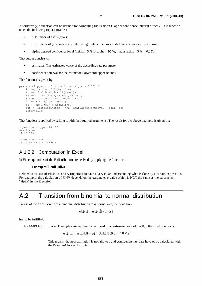
ETSI
ETSI TS 102 250-6 V1.2.1 (2004-10) 71
Alternatively, a function can be defined for computing the Pearson-Clopper confidence interval directly. This function takes the following input variables:
• n: Number of trials (total);
• m: Number of (un-)successful interesting trials, either successful ones or non-successful ones;
• alpha: desired confidence level (default: 5 % 1- alpha = 95 %, means alpha = 5 % = 0,05).
The output consists of:
• estimator: The estimated value of the according rate parameter;
• confidence interval for the estimator (lower and upper bound).
The function is given by:
pearson.clopper <- function(n, m, alpha = 0.05) { # computation of F-quantiles f1 <- qf(alpha/2,2*m,2*(n-m+1)) f2 <- qf(1-alpha/2,2*(m+1),2*(n-m)) # computation of confidence limits p1 <- m * f1/(n-m+1+m*f1) p2 <- (m+1)*f2/(n-m+(m+1)*f2) out <- list(estimator = m/n, confidence.interval = c(p1, p2)) return(out) }
The function is applied by calling it with the required arguments. The result for the above example is given by:
> pearson.clopper(40, 29) $estimator [1] 0.725 $confidence.interval [1] 0.5611171 0.8539910
A.1.2.2 Computation in Excel
In Excel, quantiles of the F-distribution are derived by applying the functions:
FINV(p-value;df1;df2)
Related to the use of Excel, it is very important to have a very clear understanding what is done by a certain expression. For example, the calculation of FINV depends on the parameter p-value which is NOT the same as the parameter "alpha" in the R section!
A.2 Transition from binomial to normal distribution To use of the transition from a binomial distribution to a normal one, the condition:
( ) 91 ≥−⋅⋅=⋅⋅ ppnqpn
has to be fulfilled.
EXAMPLE 1: If n = 30 samples are gathered which lead to an estimated rate of p = 0,8, the condition reads:
98,42,08,030)1( <=⋅⋅=−⋅⋅=⋅⋅ ppnqpn
This means, the approximation is not allowed and confidence intervals have to be calculated with the Pearson-Clopper formula.
ETSI
ETSI TS 102 250-6 V1.2.1 (2004-10) 72
EXAMPLE 2: Now, the same rate p = 0,8 is estimated on a basis of n = 300 samples. The according relation reads
9482,08,0300)1( >=⋅⋅=−⋅⋅=⋅⋅ ppnqpn
In this case, the approximation of the binomial distribution by a normal distribution is allowed. The confidence intervals can be calculated with the according expressions of the normal distribution.
A.3 Definitions of EG 201 769 The following clause presents another definition of confidence intervals related to the normal distribution. It can be found in EG 201 769-1 [1]:
• Relationship between the accuracy of estimator of the unsuccessful call ratio and the number of calls to be observed.
If k unsuccessful calls are observed out of N call attempts, then the true value of the unsuccessful call ratio lies between
∆−N
k and ∆+
N
k with a confidence level α−1 , ∆ being approximated (for large value of N) by:
N
pp )1()(
−××≈∆ ασ
where p is the expected unsuccessful call ratio and )(ασ is the 100)2
1( ×− α percentile of the normal distribution with
mean 0 and standard deviation 1 (N(0,1)). I.e. the number of call attempts to be observed should be:
2
2 )1()(
∆−×= pp
Nασ
• If the confidence level is 95,01 =−α then 296,1)( ≈=ασ .
• If the required accuracy for 01,0≤p is 001,0=∆ , then the number of call attempts to be observed should be
N = 4 × 10⁶ × p(1-p) for a confidence level of 95 %.
• If the required accuracy for p>0,01 is 1,0=∆p
, then the number of call attempts to be observed should be
N = 400 × ((1 - p)/p) for a confidence level of 95 %.
• For example, if the expected unsuccessful call ratio is 1 %, the number of call attempts to be observed should be
N = 4 × 106 × 0,01(1 - 0,01) = 39 600
for an accuracy of ∆ = 0,001 with a confidence level of 95 %.
• If the unsuccessful call ratio is expected to be 3 %, then the number of call attempts should be:
N = 400 × ((1 - 0,03)/0,03) 13 000
for a relative accuracy of 1,0=∆p
and with a confidence level of 95 %
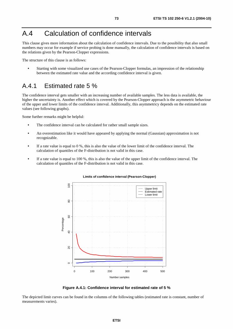
ETSI
ETSI TS 102 250-6 V1.2.1 (2004-10) 73
A.4 Calculation of confidence intervals This clause gives more information about the calculation of confidence intervals. Due to the possibility that also small numbers may occur for example if service probing is done manually, the calculation of confidence intervals is based on the relations given by the Pearson-Clopper expressions.
The structure of this clause is as follows:
• Starting with some visualized use cases of the Pearson-Clopper formulas, an impression of the relationship between the estimated rate value and the according confidence interval is given.
A.4.1 Estimated rate 5 % The confidence interval gets smaller with an increasing number of available samples. The less data is available, the higher the uncertainty is. Another effect which is covered by the Pearson-Clopper approach is the asymmetric behaviour of the upper and lower limits of the confidence interval. Additionally, this asymmetricy depends on the estimated rate values (see following graphs).
Some further remarks might be helpful:
• The confidence interval can be calculated for rather small sample sizes.
• An overestimation like it would have appeared by applying the normal (Gaussian) approximation is not recognizable.
• If a rate value is equal to 0 %, this is also the value of the lower limit of the confidence interval. The calculation of quantiles of the F-distribution is not valid in this case.
• If a rate value is equal to 100 %, this is also the value of the upper limit of the confidence interval. The calculation of quantiles of the F-distribution is not valid in this case.
0 100 200 300 400 500
020
4060
8010
0
Limits of confidence interval (Pearson-Clopper)
Number samples
Per
cent
age
Upper limitEstimated rateLower limit
Figure A.4.1: Confidence interval for estimated rate of 5 %
The depicted limit curves can be found in the columns of the following tables (estimated rate is constant, number of measurements varies).
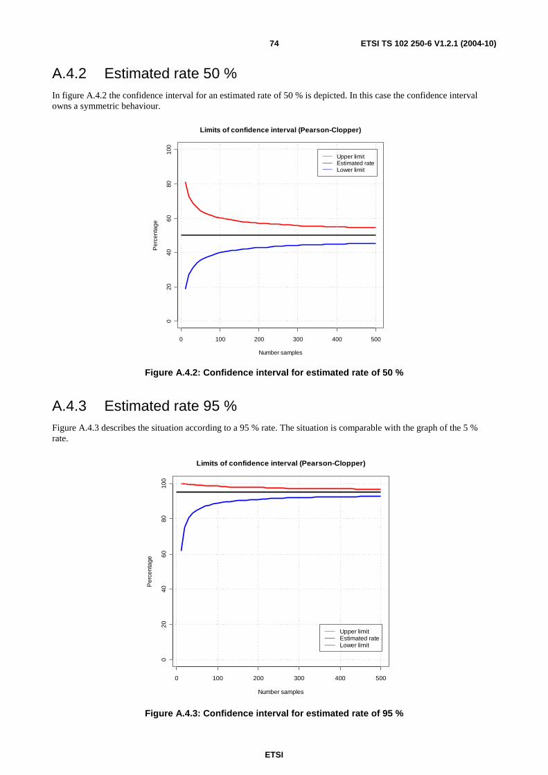
ETSI
ETSI TS 102 250-6 V1.2.1 (2004-10) 74
A.4.2 Estimated rate 50 % In figure A.4.2 the confidence interval for an estimated rate of 50 % is depicted. In this case the confidence interval owns a symmetric behaviour.
0 100 200 300 400 500
020
4060
8010
0
Limits of confidence interval (Pearson-Clopper)
Number samples
Per
cent
age
Upper limitEstimated rateLower limit
Figure A.4.2: Confidence interval for estimated rate of 50 %
A.4.3 Estimated rate 95 % Figure A.4.3 describes the situation according to a 95 % rate. The situation is comparable with the graph of the 5 % rate.
0 100 200 300 400 500
020
4060
8010
0
Limits of confidence interval (Pearson-Clopper)
Number samples
Per
cent
age
Upper limitEstimated rateLower limit
Figure A.4.3: Confidence interval for estimated rate of 95 %
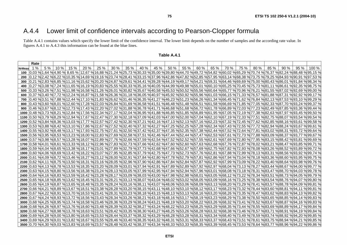
ETSI
ETSI TS 102 250-6 V1.2.1 (2004-10) 75
A.4.4 Lower limit of confidence intervals according to Pearson-Clopper formula Table A.4.1 contains values which specify the lower limit of the confidence interval. The lower limit depends on the number of samples and the according rate value. In figures A.4.1 to A.4.3 this information can be found at the blue lines.
Table A.4.1
Rate NrMeas 1 % 5 % 10 % 15 % 20 % 25 % 30 % 35 % 40 % 45 % 50 % 55 % 60 % 65 % 70 % 75 % 80 % 85 % 90 % 95 % 100 %
100 0,03 % 1,64 % 4,90 % 8,65 % 12,67 %16,88 % 21,24 % 25,73 % 30,33 %35,00 % 39,80 % 44,70 % 49,72 %54,82 % 60,02 % 65,29 % 70,74 % 76,37 % 82,24 %88,48 % 95,15 %200 0,12 % 2,42 % 6,22 %10,35 % 14,69 %19,16 % 23,74 % 28,41 % 33,15 %37,96 % 42,86 % 47,82 % 52,85 %57,95 % 63,14 % 68,38 % 73,75 % 79,25 % 84,93 %90,91 % 97,53 %300 0,21 % 2,83 % 6,85 %11,16 % 15,62 %20,20 % 24,87 % 29,61 % 34,41 %39,28 % 44,19 % 49,17 % 54,21 %59,31 % 64,46 % 69,69 % 75,00 % 80,43 % 86,01 %91,84 % 98,34 %400 0,27 % 3,08 % 7,24 %11,65 % 16,19 %20,83 % 25,55 % 30,33 % 35,16 %40,05 % 44,99 % 49,98 % 55,01 %60,10 % 65,25 % 70,45 % 75,73 % 81,11 % 86,61 %92,35 % 98,75 %500 0,33 % 3,26 % 7,51 %11,98 % 16,58 %21,26 % 26,01 % 30,82 % 35,67 %40,58 % 45,53 % 50,52 % 55,56 %60,64 % 65,77 % 70,96 % 76,21 % 81,55 % 87,02 %92,69 % 99,00 %600 0,37 % 3,40 % 7,72 %12,24 % 16,87 %21,58 % 26,36 % 31,18 % 36,05 %40,97 % 45,92 % 50,92 % 55,96 %61,03 % 66,15 % 71,33 % 76,57 % 81,88 % 87,31 %92,92 % 99,17 %700 0,40 % 3,51 % 7,88 %12,44 % 17,10 %21,83 % 26,62 % 31,46 % 36,35 %41,27 % 46,23 % 51,23 % 56,26 %61,34 % 66,45 % 71,62 % 76,84 % 82,13 % 87,53 %93,10 % 99,29 %800 0,43 % 3,60 % 8,01 %12,60 % 17,28 %22,03 % 26,84 % 31,69 % 36,58 %41,51 % 46,48 % 51,48 % 56,51 %61,58 % 66,69 % 71,85 % 77,05 % 82,33 % 87,70 %93,24 % 99,37 %900 0,46 % 3,67 % 8,12 %12,73 % 17,43 %22,20 % 27,02 % 31,88 % 36,78 %41,71 % 46,68 % 51,68 % 56,72 %61,78 % 66,89 % 72,03 % 77,23 % 82,49 % 87,85 %93,36 % 99,44 %
1000 0,48 % 3,73 % 8,21 %12,84 % 17,56 %22,34 % 27,17 % 32,04 % 36,95 %41,88 % 46,85 % 51,85 % 56,89 %61,95 % 67,05 % 72,19 % 77,38 % 82,63 % 87,97 %93,45 % 99,50 %1100 0,50 % 3,79 % 8,29 %12,94 % 17,67 %22,47 % 27,30 % 32,18 % 37,09 %42,03 % 47,00 % 52,00 % 57,04 %62,10 % 67,19 % 72,33 % 77,51 % 82,75 % 88,07 %93,54 % 99,54 %1200 0,52 % 3,84 % 8,36 %13,03 % 17,77 %22,57 % 27,42 % 32,30 % 37,21 %42,16 % 47,13 % 52,13 % 57,16 %62,23 % 67,32 % 72,45 % 77,62 % 82,85 % 88,16 %93,61 % 99,58 %1300 0,53 % 3,88 % 8,42 %13,10 % 17,86 %22,67 % 27,52 % 32,40 % 37,32 %42,27 % 47,25 % 52,25 % 57,28 %62,34 % 67,43 % 72,55 % 77,72 % 82,94 % 88,24 %93,67 % 99,61 %1400 0,55 % 3,92 % 8,48 %13,17 % 17,93 %22,75 % 27,61 % 32,50 % 37,42 %42,37 % 47,35 % 52,35 % 57,38 %62,44 % 67,52 % 72,64 % 77,81 % 83,02 % 88,31 %93,72 % 99,64 %1500 0,56 % 3,95 % 8,53 %13,23 % 18,00 %22,83 % 27,69 % 32,58 % 37,51 %42,46 % 47,44 % 52,44 % 57,47 %62,53 % 67,61 % 72,73 % 77,88 % 83,09 % 88,37 %93,77 % 99,67 %1600 0,57 % 3,98 % 8,57 %13,28 % 18,07 %22,89 % 27,76 % 32,66 % 37,59 %42,54 % 47,52 % 52,52 % 57,55 %62,61 % 67,69 % 72,80 % 77,95 % 83,15 % 88,42 %93,81 % 99,69 %1700 0,58 % 4,01 % 8,61 %13,33 % 18,12 %22,96 % 27,83 % 32,73 % 37,66 %42,62 % 47,60 % 52,60 % 57,63 %62,68 % 67,76 % 72,87 % 78,02 % 83,21 % 88,47 %93,85 % 99,71 %1800 0,59 % 4,04 % 8,65 %13,38 % 18,17 %23,01 % 27,89 % 32,79 % 37,73 %42,68 % 47,66 % 52,67 % 57,69 %62,75 % 67,82 % 72,93 % 78,08 % 83,26 % 88,52 %93,89 % 99,72 %1900 0,60 % 4,06 % 8,69 %13,42 % 18,22 %23,07 % 27,95 % 32,85 % 37,79 %42,75 % 47,73 % 52,73 % 57,76 %62,81 % 67,88 % 72,99 % 78,13 % 83,31 % 88,56 %93,92 % 99,74 %2000 0,61 % 4,09 % 8,72 %13,46 % 18,27 %23,12 % 28,00 % 32,91 % 37,84 %42,80 % 47,78 % 52,79 % 57,81 %62,86 % 67,94 % 73,04 % 78,18 % 83,36 % 88,60 %93,95 % 99,75 %2100 0,62 % 4,11 % 8,75 %13,50 % 18,31 %23,16 % 28,05 % 32,96 % 37,90 %42,86 % 47,84 % 52,84 % 57,87 %62,92 % 67,99 % 73,09 % 78,22 % 83,40 % 88,64 %93,98 % 99,76 %2200 0,63 % 4,13 % 8,78 %13,53 % 18,35 %23,20 % 28,09 % 33,01 % 37,94 %42,91 % 47,89 % 52,89 % 57,92 %62,97 % 68,04 % 73,13 % 78,27 % 83,44 % 88,67 %94,00 % 99,77 %2300 0,63 % 4,15 % 8,80 %13,56 % 18,38 %23,24 % 28,13 % 33,05 % 37,99 %42,95 % 47,94 % 52,94 % 57,96 %63,01 % 68,08 % 73,18 % 78,31 % 83,47 % 88,70 %94,03 % 99,78 %2400 0,64 % 4,16 % 8,83 %13,59 % 18,42 %23,28 % 28,17 % 33,09 % 38,03 %43,00 % 47,98 % 52,98 % 58,01 %63,05 % 68,12 % 73,22 % 78,34 % 83,51 % 88,73 %94,05 % 99,79 %2500 0,65 % 4,18 % 8,85 %13,62 % 18,45 %23,31 % 28,21 % 33,13 % 38,07 %43,04 % 48,02 % 53,02 % 58,05 %63,09 % 68,16 % 73,25 % 78,38 % 83,54 % 88,76 %94,07 % 99,80 %2600 0,65 % 4,19 % 8,87 %13,65 % 18,48 %23,35 % 28,24 % 33,16 % 38,11 %43,07 % 48,06 % 53,06 % 58,09 %63,13 % 68,20 % 73,29 % 78,41 % 83,57 % 88,78 %94,09 % 99,81 %2700 0,66 % 4,21 % 8,89 %13,67 % 18,51 %23,38 % 28,28 % 33,20 % 38,15 %43,11 % 48,10 % 53,10 % 58,12 %63,17 % 68,23 % 73,32 % 78,44 % 83,60 % 88,81 %94,11 % 99,81 %2800 0,67 % 4,22 % 8,91 %13,70 % 18,53 %23,41 % 28,31 % 33,23 % 38,18 %43,15 % 48,13 % 53,13 % 58,16 %63,20 % 68,26 % 73,35 % 78,47 % 83,62 % 88,83 %94,13 % 99,82 %2900 0,67 % 4,24 % 8,93 %13,72 % 18,56 %23,43 % 28,34 % 33,26 % 38,21 %43,18 % 48,16 % 53,17 % 58,19 %63,23 % 68,29 % 73,38 % 78,50 % 83,65 % 88,85 %94,14 % 99,83 %3000 0,68 % 4,25 % 8,95 %13,74 % 18,58 %23,46 % 28,36 % 33,29 % 38,24 %43,21 % 48,19 % 53,20 % 58,22 %63,26 % 68,32 % 73,41 % 78,52 % 83,67 % 88,87 %94,16 % 99,83 %3100 0,68 % 4,26 % 8,97 %13,76 % 18,60 %23,48 % 28,39 % 33,32 % 38,27 %43,24 % 48,22 % 53,23 % 58,25 %63,29 % 68,35 % 73,44 % 78,55 % 83,69 % 88,89 %94,17 % 99,84 %3200 0,68 % 4,27 % 8,98 %13,78 % 18,63 %23,51 % 28,42 % 33,35 % 38,30 %43,27 % 48,25 % 53,26 % 58,28 %63,32 % 68,38 % 73,46 % 78,57 % 83,71 % 88,91 %94,19 % 99,84 %3300 0,69 % 4,28 % 9,00 %13,80 % 18,65 %23,53 % 28,44 % 33,37 % 38,32 %43,29 % 48,28 % 53,28 % 58,31 %63,34 % 68,40 % 73,49 % 78,59 % 83,74 % 88,92 %94,20 % 99,85 %3400 0,69 % 4,29 % 9,01 %13,82 % 18,67 %23,55 % 28,46 % 33,40 % 38,35 %43,32 % 48,31 % 53,31 % 58,33 %63,37 % 68,43 % 73,51 % 78,61 % 83,75 % 88,94 %94,21 % 99,85 %3500 0,70 % 4,30 % 9,03 %13,83 % 18,69 %23,57 % 28,48 % 33,42 % 38,37 %43,34 % 48,33 % 53,33 % 58,35 %63,39 % 68,45 % 73,53 % 78,64 % 83,77 % 88,96 %94,22 % 99,86 %
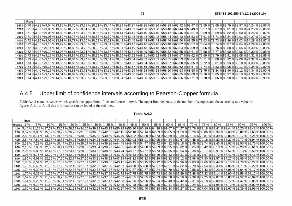
ETSI
ETSI TS 102 250-6 V1.2.1 (2004-10) 76
Rate 3600 0,70 % 4,31 % 9,04 %13,85 % 18,70 %23,59 % 28,51 % 33,44 % 38,39 %43,37 % 48,35 % 53,36 % 58,38 %63,42 % 68,47 % 73,55 % 78,65 % 83,79 % 88,97 %94,24 % 99,86 %3700 0,71 % 4,32 % 9,05 %13,86 % 18,72 %23,61 % 28,53 % 33,46 % 38,42 %43,39 % 48,38 % 53,38 % 58,40 %63,44 % 68,49 % 73,57 % 78,67 % 83,81 % 88,99 %94,25 % 99,86 %3800 0,71 % 4,33 % 9,06 %13,88 % 18,74 %23,63 % 28,55 % 33,48 % 38,44 %43,41 % 48,40 % 53,40 % 58,42 %63,46 % 68,51 % 73,59 % 78,69 % 83,82 % 89,00 %94,26 % 99,87 %3900 0,71 % 4,34 % 9,08 %13,89 % 18,75 %23,65 % 28,56 % 33,50 % 38,46 %43,43 % 48,42 % 53,42 % 58,44 %63,48 % 68,53 % 73,61 % 78,71 % 83,84 % 89,01 %94,27 % 99,87 %4000 0,72 % 4,35 % 9,09 %13,91 % 18,77 %23,66 % 28,58 % 33,52 % 38,48 %43,45 % 48,44 % 53,44 % 58,46 %63,50 % 68,55 % 73,63 % 78,73 % 83,86 % 89,03 %94,28 % 99,87 %4100 0,72 % 4,35 % 9,10 %13,92 % 18,79 %23,68 % 28,60 % 33,54 % 38,50 %43,47 % 48,46 % 53,46 % 58,48 %63,52 % 68,57 % 73,64 % 78,74 % 83,87 % 89,04 %94,29 % 99,88 %4200 0,72 % 4,36 % 9,11 %13,93 % 18,80 %23,70 % 28,62 % 33,56 % 38,51 %43,49 % 48,48 % 53,48 % 58,50 %63,54 % 68,59 % 73,66 % 78,76 % 83,88 % 89,05 %94,30 % 99,88 %4300 0,72 % 4,37 % 9,12 %13,95 % 18,81 %23,71 % 28,63 % 33,57 % 38,53 %43,51 % 48,49 % 53,50 % 58,52 %63,55 % 68,61 % 73,68 % 78,77 % 83,90 % 89,06 %94,30 % 99,88 %4400 0,73 % 4,37 % 9,13 %13,96 % 18,83 %23,73 % 28,65 % 33,59 % 38,55 %43,52 % 48,51 % 53,52 % 58,53 %63,57 % 68,62 % 73,69 % 78,79 % 83,91 % 89,08 %94,31 % 99,89 %4500 0,73 % 4,38 % 9,14 %13,97 % 18,84 %23,74 % 28,66 % 33,61 % 38,56 %43,54 % 48,53 % 53,53 % 58,55 %63,59 % 68,64 % 73,71 % 78,80 % 83,92 % 89,09 %94,32 % 99,89 %4600 0,73 % 4,39 % 9,15 %13,98 % 18,85 %23,75 % 28,68 % 33,62 % 38,58 %43,56 % 48,54 % 53,55 % 58,57 %63,60 % 68,65 % 73,72 % 78,81 % 83,93 % 89,10 %94,33 % 99,89 %4700 0,74 % 4,39 % 9,16 %13,99 % 18,86 %23,77 % 28,69 % 33,64 % 38,60 %43,57 % 48,56 % 53,56 % 58,58 %63,62 % 68,67 % 73,74 % 78,83 % 83,95 % 89,11 %94,34 % 99,89 %4800 0,74 % 4,40 % 9,17 %14,00 % 18,88 %23,78 % 28,71 % 33,65 % 38,61 %43,59 % 48,58 % 53,58 % 58,60 %63,63 % 68,68 % 73,75 % 78,84 % 83,96 % 89,12 %94,34 % 99,90 %4900 0,74 % 4,41 % 9,17 %14,01 % 18,89 %23,79 % 28,72 % 33,66 % 38,62 %43,60 % 48,59 % 53,59 % 58,61 %63,65 % 68,69 % 73,76 % 78,85 % 83,97 % 89,13 %94,35 % 99,90 %5000 0,74 % 4,41 % 9,18 %14,02 % 18,90 %23,80 % 28,73 % 33,68 % 38,64 %43,61 % 48,60 % 53,61 % 58,63 %63,66 % 68,71 % 73,78 % 78,86 % 83,98 % 89,13 %94,36 % 99,90 %
A.4.5 Upper limit of confidence intervals according to Pearson-Clopper formula Table A.4.2 contains values which specify the upper limit of the confidence interval. The upper limit depends on the number of samples and the according rate value. In figures A.4.1 to A.4.3 this information can be found at the red lines.
Table A.4.2
Rate NrMeas 1 % 5 % 10 % 15 % 20 % 25 % 30 % 35 % 40 % 45 % 50 % 55 % 60 % 65 % 70 % 75 % 80 % 85 % 90 % 95 % 100 %
100 5,45 % 11,28 % 17,62 %23,53 % 29,18 % 34,66 % 39,98 % 45,18 % 50,28 %55,30 % 60,19 % 64,98 % 69,67 %74,27 % 78,76 % 83,18 % 87,41 %91,44 % 95,20 %98,48 % 100,00 %200 3,57 % 9,00 % 15,02 %20,72 % 26,22 % 31,60 % 36,87 % 42,05 % 47,15 %52,18 % 57,14 % 62,03 % 66,85 %71,59 % 76,26 % 80,86 % 85,34 %89,68 % 93,82 %97,63 % 100,00 %300 2,89 % 8,11 % 13,97 %19,55 % 24,98 % 30,30 % 35,53 % 40,69 % 45,79 %50,82 % 55,80 % 60,73 % 65,59 %70,39 % 75,14 % 79,81 % 84,39 %88,86 % 93,17 %97,21 % 100,00 %400 2,54 % 7,62 % 13,37 %18,88 % 24,26 % 29,54 % 34,75 % 39,90 % 44,99 %50,03 % 55,01 % 59,95 % 64,84 %69,67 % 74,45 % 79,18 % 83,82 %88,37 % 92,77 %96,94 % 100,00 %500 2,32 % 7,29 % 12,97 %18,44 % 23,78 % 29,04 % 34,23 % 39,36 % 44,45 %49,48 % 54,47 % 59,42 % 64,32 %69,18 % 73,99 % 78,74 % 83,43 %88,02 % 92,50 %96,75 % 100,00 %600 2,16 % 7,06 % 12,68 %18,11 % 23,43 % 28,67 % 33,84 % 38,97 % 44,05 %49,08 % 54,08 % 59,03 % 63,95 %68,82 % 73,65 % 78,42 % 83,13 %87,77 % 92,29 %96,61 % 100,00 %700 2,05 % 6,89 % 12,47 %17,86 % 23,16 % 28,38 % 33,55 % 38,66 % 43,74 %48,77 % 53,77 % 58,73 % 63,65 %68,54 % 73,38 % 78,17 % 82,91 %87,57 % 92,13 %96,50 % 100,00 %800 1,96 % 6,75 % 12,29 %17,67 % 22,94 % 28,15 % 33,31 % 38,42 % 43,49 %48,52 % 53,52 % 58,49 % 63,42 %68,31 % 73,16 % 77,97 % 82,72 %87,41 % 92,00 %96,41 % 100,00 %900 1,89 % 6,63 % 12,15 %17,50 % 22,77 % 27,96 % 33,11 % 38,22 % 43,29 %48,32 % 53,32 % 58,29 % 63,22 %68,12 % 72,98 % 77,80 % 82,57 %87,27 % 91,89 %96,34 % 100,00 %
1000 1,83 % 6,54 % 12,03 %17,37 % 22,62 % 27,81 % 32,95 % 38,05 % 43,11 %48,15 % 53,15 % 58,12 % 63,05 %67,96 % 72,83 % 77,66 % 82,44 %87,16 % 91,79 %96,27 % 100,00 %1100 1,78 % 6,46 % 11,93 %17,25 % 22,49 % 27,67 % 32,80 % 37,90 % 42,97 %48,00 % 53,00 % 57,97 % 62,91 %67,82 % 72,70 % 77,54 % 82,33 %87,06 % 91,71 %96,22 % 100,00 %1200 1,74 % 6,39 % 11,84 %17,15 % 22,38 % 27,55 % 32,68 % 37,77 % 42,84 %47,87 % 52,87 % 57,84 % 62,79 %67,70 % 72,58 % 77,43 % 82,23 %86,98 % 91,64 %96,17 % 100,00 %1300 1,70 % 6,33 % 11,76 %17,06 % 22,28 % 27,45 % 32,57 % 37,66 % 42,72 %47,75 % 52,75 % 57,73 % 62,68 %67,59 % 72,48 % 77,33 % 82,14 %86,90 % 91,58 %96,12 % 100,00 %1400 1,67 % 6,28 % 11,69 %16,98 % 22,19 % 27,35 % 32,48 % 37,56 % 42,62 %47,65 % 52,65 % 57,63 % 62,58 %67,50 % 72,39 % 77,25 % 82,07 %86,83 % 91,52 %96,09 % 100,00 %1500 1,64 % 6,23 % 11,63 %16,91 % 22,12 % 27,27 % 32,39 % 37,47 % 42,53 %47,56 % 52,56 % 57,54 % 62,49 %67,42 % 72,31 % 77,18 % 82,00 %86,77 % 91,47 %96,05 % 100,00 %1600 1,62 % 6,18 % 11,58 %16,84 % 22,05 % 27,20 % 32,31 % 37,39 % 42,45 %47,48 % 52,48 % 57,46 % 62,41 %67,34 % 72,24 % 77,11 % 81,94 %86,72 % 91,43 %96,02 % 100,00 %1700 1,60 % 6,15 % 11,53 %16,79 % 21,98 % 27,13 % 32,24 % 37,32 % 42,37 %47,40 % 52,40 % 57,38 % 62,34 %67,27 % 72,17 % 77,04 % 81,88 %86,67 % 91,39 %95,99 % 100,00 %
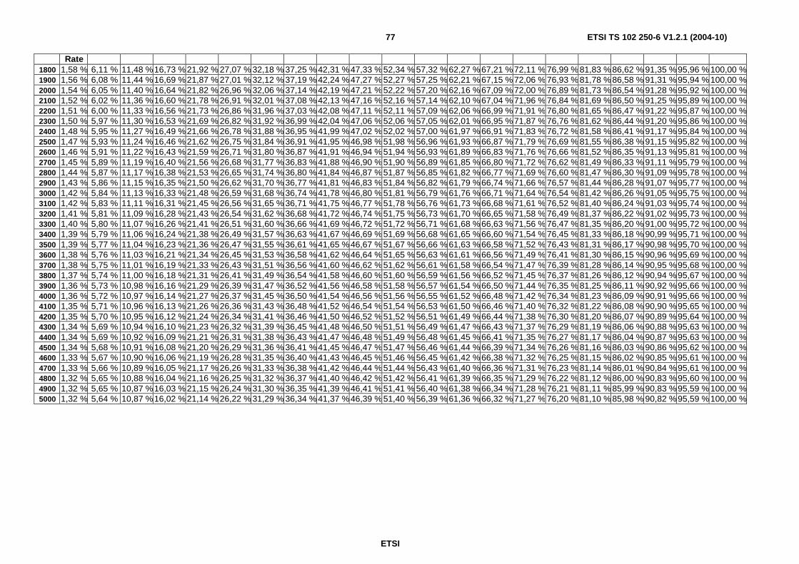
ETSI
ETSI TS 102 250-6 V1.2.1 (2004-10) 77
Rate 1800 1,58 % 6,11 % 11,48 %16,73 % 21,92 % 27,07 % 32,18 % 37,25 % 42,31 %47,33 % 52,34 % 57,32 % 62,27 %67,21 % 72,11 % 76,99 % 81,83 %86,62 % 91,35 %95,96 % 100,00 %1900 1,56 % 6,08 % 11,44 %16,69 % 21,87 % 27,01 % 32,12 % 37,19 % 42,24 %47,27 % 52,27 % 57,25 % 62,21 %67,15 % 72,06 % 76,93 % 81,78 %86,58 % 91,31 %95,94 % 100,00 %2000 1,54 % 6,05 % 11,40 %16,64 % 21,82 % 26,96 % 32,06 % 37,14 % 42,19 %47,21 % 52,22 % 57,20 % 62,16 %67,09 % 72,00 % 76,89 % 81,73 %86,54 % 91,28 %95,92 % 100,00 %2100 1,52 % 6,02 % 11,36 %16,60 % 21,78 % 26,91 % 32,01 % 37,08 % 42,13 %47,16 % 52,16 % 57,14 % 62,10 %67,04 % 71,96 % 76,84 % 81,69 %86,50 % 91,25 %95,89 % 100,00 %2200 1,51 % 6,00 % 11,33 %16,56 % 21,73 % 26,86 % 31,96 % 37,03 % 42,08 %47,11 % 52,11 % 57,09 % 62,06 %66,99 % 71,91 % 76,80 % 81,65 %86,47 % 91,22 %95,87 % 100,00 %2300 1,50 % 5,97 % 11,30 %16,53 % 21,69 % 26,82 % 31,92 % 36,99 % 42,04 %47,06 % 52,06 % 57,05 % 62,01 %66,95 % 71,87 % 76,76 % 81,62 %86,44 % 91,20 %95,86 % 100,00 %2400 1,48 % 5,95 % 11,27 %16,49 % 21,66 % 26,78 % 31,88 % 36,95 % 41,99 %47,02 % 52,02 % 57,00 % 61,97 %66,91 % 71,83 % 76,72 % 81,58 %86,41 % 91,17 %95,84 % 100,00 %2500 1,47 % 5,93 % 11,24 %16,46 % 21,62 % 26,75 % 31,84 % 36,91 % 41,95 %46,98 % 51,98 % 56,96 % 61,93 %66,87 % 71,79 % 76,69 % 81,55 %86,38 % 91,15 %95,82 % 100,00 %2600 1,46 % 5,91 % 11,22 %16,43 % 21,59 % 26,71 % 31,80 % 36,87 % 41,91 %46,94 % 51,94 % 56,93 % 61,89 %66,83 % 71,76 % 76,66 % 81,52 %86,35 % 91,13 %95,81 % 100,00 %2700 1,45 % 5,89 % 11,19 %16,40 % 21,56 % 26,68 % 31,77 % 36,83 % 41,88 %46,90 % 51,90 % 56,89 % 61,85 %66,80 % 71,72 % 76,62 % 81,49 %86,33 % 91,11 %95,79 % 100,00 %2800 1,44 % 5,87 % 11,17 %16,38 % 21,53 % 26,65 % 31,74 % 36,80 % 41,84 %46,87 % 51,87 % 56,85 % 61,82 %66,77 % 71,69 % 76,60 % 81,47 %86,30 % 91,09 %95,78 % 100,00 %2900 1,43 % 5,86 % 11,15 %16,35 % 21,50 % 26,62 % 31,70 % 36,77 % 41,81 %46,83 % 51,84 % 56,82 % 61,79 %66,74 % 71,66 % 76,57 % 81,44 %86,28 % 91,07 %95,77 % 100,00 %3000 1,42 % 5,84 % 11,13 %16,33 % 21,48 % 26,59 % 31,68 % 36,74 % 41,78 %46,80 % 51,81 % 56,79 % 61,76 %66,71 % 71,64 % 76,54 % 81,42 %86,26 % 91,05 %95,75 % 100,00 %3100 1,42 % 5,83 % 11,11 %16,31 % 21,45 % 26,56 % 31,65 % 36,71 % 41,75 %46,77 % 51,78 % 56,76 % 61,73 %66,68 % 71,61 % 76,52 % 81,40 %86,24 % 91,03 %95,74 % 100,00 %3200 1,41 % 5,81 % 11,09 %16,28 % 21,43 % 26,54 % 31,62 % 36,68 % 41,72 %46,74 % 51,75 % 56,73 % 61,70 %66,65 % 71,58 % 76,49 % 81,37 %86,22 % 91,02 %95,73 % 100,00 %3300 1,40 % 5,80 % 11,07 %16,26 % 21,41 % 26,51 % 31,60 % 36,66 % 41,69 %46,72 % 51,72 % 56,71 % 61,68 %66,63 % 71,56 % 76,47 % 81,35 %86,20 % 91,00 %95,72 % 100,00 %3400 1,39 % 5,79 % 11,06 %16,24 % 21,38 % 26,49 % 31,57 % 36,63 % 41,67 %46,69 % 51,69 % 56,68 % 61,65 %66,60 % 71,54 % 76,45 % 81,33 %86,18 % 90,99 %95,71 % 100,00 %3500 1,39 % 5,77 % 11,04 %16,23 % 21,36 % 26,47 % 31,55 % 36,61 % 41,65 %46,67 % 51,67 % 56,66 % 61,63 %66,58 % 71,52 % 76,43 % 81,31 %86,17 % 90,98 %95,70 % 100,00 %3600 1,38 % 5,76 % 11,03 %16,21 % 21,34 % 26,45 % 31,53 % 36,58 % 41,62 %46,64 % 51,65 % 56,63 % 61,61 %66,56 % 71,49 % 76,41 % 81,30 %86,15 % 90,96 %95,69 % 100,00 %3700 1,38 % 5,75 % 11,01 %16,19 % 21,33 % 26,43 % 31,51 % 36,56 % 41,60 %46,62 % 51,62 % 56,61 % 61,58 %66,54 % 71,47 % 76,39 % 81,28 %86,14 % 90,95 %95,68 % 100,00 %3800 1,37 % 5,74 % 11,00 %16,18 % 21,31 % 26,41 % 31,49 % 36,54 % 41,58 %46,60 % 51,60 % 56,59 % 61,56 %66,52 % 71,45 % 76,37 % 81,26 %86,12 % 90,94 %95,67 % 100,00 %3900 1,36 % 5,73 % 10,98 %16,16 % 21,29 % 26,39 % 31,47 % 36,52 % 41,56 %46,58 % 51,58 % 56,57 % 61,54 %66,50 % 71,44 % 76,35 % 81,25 %86,11 % 90,92 %95,66 % 100,00 %4000 1,36 % 5,72 % 10,97 %16,14 % 21,27 % 26,37 % 31,45 % 36,50 % 41,54 %46,56 % 51,56 % 56,55 % 61,52 %66,48 % 71,42 % 76,34 % 81,23 %86,09 % 90,91 %95,66 % 100,00 %4100 1,35 % 5,71 % 10,96 %16,13 % 21,26 % 26,36 % 31,43 % 36,48 % 41,52 %46,54 % 51,54 % 56,53 % 61,50 %66,46 % 71,40 % 76,32 % 81,22 %86,08 % 90,90 %95,65 % 100,00 %4200 1,35 % 5,70 % 10,95 %16,12 % 21,24 % 26,34 % 31,41 % 36,46 % 41,50 %46,52 % 51,52 % 56,51 % 61,49 %66,44 % 71,38 % 76,30 % 81,20 %86,07 % 90,89 %95,64 % 100,00 %4300 1,34 % 5,69 % 10,94 %16,10 % 21,23 % 26,32 % 31,39 % 36,45 % 41,48 %46,50 % 51,51 % 56,49 % 61,47 %66,43 % 71,37 % 76,29 % 81,19 %86,06 % 90,88 %95,63 % 100,00 %4400 1,34 % 5,69 % 10,92 %16,09 % 21,21 % 26,31 % 31,38 % 36,43 % 41,47 %46,48 % 51,49 % 56,48 % 61,45 %66,41 % 71,35 % 76,27 % 81,17 %86,04 % 90,87 %95,63 % 100,00 %4500 1,34 % 5,68 % 10,91 %16,08 % 21,20 % 26,29 % 31,36 % 36,41 % 41,45 %46,47 % 51,47 % 56,46 % 61,44 %66,39 % 71,34 % 76,26 % 81,16 %86,03 % 90,86 %95,62 % 100,00 %4600 1,33 % 5,67 % 10,90 %16,06 % 21,19 % 26,28 % 31,35 % 36,40 % 41,43 %46,45 % 51,46 % 56,45 % 61,42 %66,38 % 71,32 % 76,25 % 81,15 %86,02 % 90,85 %95,61 % 100,00 %4700 1,33 % 5,66 % 10,89 %16,05 % 21,17 % 26,26 % 31,33 % 36,38 % 41,42 %46,44 % 51,44 % 56,43 % 61,40 %66,36 % 71,31 % 76,23 % 81,14 %86,01 % 90,84 %95,61 % 100,00 %4800 1,32 % 5,65 % 10,88 %16,04 % 21,16 % 26,25 % 31,32 % 36,37 % 41,40 %46,42 % 51,42 % 56,41 % 61,39 %66,35 % 71,29 % 76,22 % 81,12 %86,00 % 90,83 %95,60 % 100,00 %4900 1,32 % 5,65 % 10,87 %16,03 % 21,15 % 26,24 % 31,30 % 36,35 % 41,39 %46,41 % 51,41 % 56,40 % 61,38 %66,34 % 71,28 % 76,21 % 81,11 %85,99 % 90,83 %95,59 % 100,00 %5000 1,32 % 5,64 % 10,87 %16,02 % 21,14 % 26,22 % 31,29 % 36,34 % 41,37 %46,39 % 51,40 % 56,39 % 61,36 %66,32 % 71,27 % 76,20 % 81,10 %85,98 % 90,82 %95,59 % 100,00 %
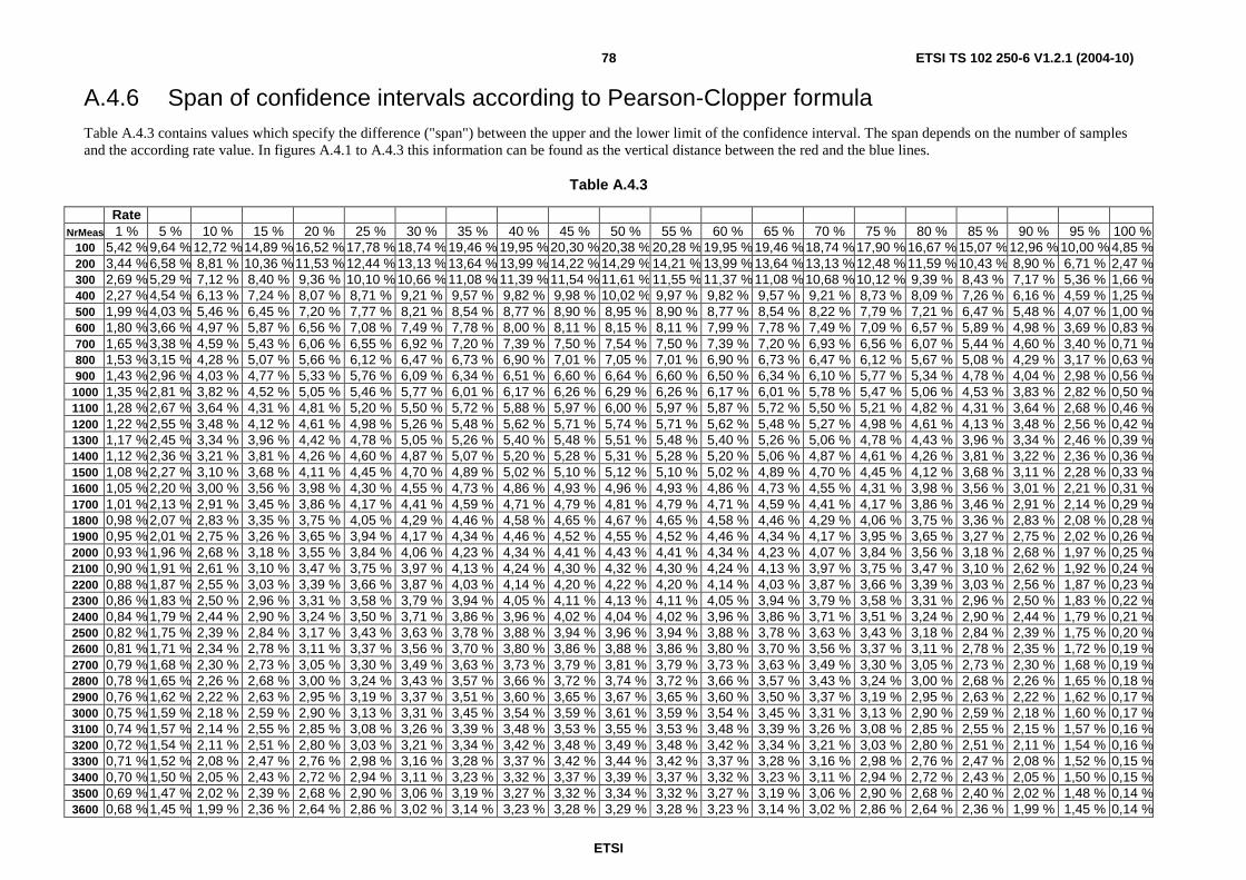
ETSI
ETSI TS 102 250-6 V1.2.1 (2004-10) 78
A.4.6 Span of confidence intervals according to Pearson-Clopper formula Table A.4.3 contains values which specify the difference ("span") between the upper and the lower limit of the confidence interval. The span depends on the number of samples and the according rate value. In figures A.4.1 to A.4.3 this information can be found as the vertical distance between the red and the blue lines.
Table A.4.3
Rate NrMeas 1 % 5 % 10 % 15 % 20 % 25 % 30 % 35 % 40 % 45 % 50 % 55 % 60 % 65 % 70 % 75 % 80 % 85 % 90 % 95 % 100 %
100 5,42 % 9,64 % 12,72 %14,89 % 16,52 % 17,78 % 18,74 %19,46 % 19,95 %20,30 % 20,38 % 20,28 % 19,95 % 19,46 %18,74 % 17,90 % 16,67 % 15,07 %12,96 % 10,00 % 4,85 %200 3,44 % 6,58 % 8,81 % 10,36 % 11,53 % 12,44 % 13,13 %13,64 % 13,99 %14,22 % 14,29 % 14,21 % 13,99 % 13,64 %13,13 % 12,48 % 11,59 % 10,43 % 8,90 % 6,71 % 2,47 %300 2,69 % 5,29 % 7,12 % 8,40 % 9,36 % 10,10 % 10,66 %11,08 % 11,39 %11,54 % 11,61 % 11,55 % 11,37 % 11,08 %10,68 % 10,12 % 9,39 % 8,43 % 7,17 % 5,36 % 1,66 %400 2,27 % 4,54 % 6,13 % 7,24 % 8,07 % 8,71 % 9,21 % 9,57 % 9,82 % 9,98 % 10,02 % 9,97 % 9,82 % 9,57 % 9,21 % 8,73 % 8,09 % 7,26 % 6,16 % 4,59 % 1,25 %500 1,99 % 4,03 % 5,46 % 6,45 % 7,20 % 7,77 % 8,21 % 8,54 % 8,77 % 8,90 % 8,95 % 8,90 % 8,77 % 8,54 % 8,22 % 7,79 % 7,21 % 6,47 % 5,48 % 4,07 % 1,00 %600 1,80 % 3,66 % 4,97 % 5,87 % 6,56 % 7,08 % 7,49 % 7,78 % 8,00 % 8,11 % 8,15 % 8,11 % 7,99 % 7,78 % 7,49 % 7,09 % 6,57 % 5,89 % 4,98 % 3,69 % 0,83 %700 1,65 % 3,38 % 4,59 % 5,43 % 6,06 % 6,55 % 6,92 % 7,20 % 7,39 % 7,50 % 7,54 % 7,50 % 7,39 % 7,20 % 6,93 % 6,56 % 6,07 % 5,44 % 4,60 % 3,40 % 0,71 %800 1,53 % 3,15 % 4,28 % 5,07 % 5,66 % 6,12 % 6,47 % 6,73 % 6,90 % 7,01 % 7,05 % 7,01 % 6,90 % 6,73 % 6,47 % 6,12 % 5,67 % 5,08 % 4,29 % 3,17 % 0,63 %900 1,43 % 2,96 % 4,03 % 4,77 % 5,33 % 5,76 % 6,09 % 6,34 % 6,51 % 6,60 % 6,64 % 6,60 % 6,50 % 6,34 % 6,10 % 5,77 % 5,34 % 4,78 % 4,04 % 2,98 % 0,56 %
1000 1,35 % 2,81 % 3,82 % 4,52 % 5,05 % 5,46 % 5,77 % 6,01 % 6,17 % 6,26 % 6,29 % 6,26 % 6,17 % 6,01 % 5,78 % 5,47 % 5,06 % 4,53 % 3,83 % 2,82 % 0,50 %1100 1,28 % 2,67 % 3,64 % 4,31 % 4,81 % 5,20 % 5,50 % 5,72 % 5,88 % 5,97 % 6,00 % 5,97 % 5,87 % 5,72 % 5,50 % 5,21 % 4,82 % 4,31 % 3,64 % 2,68 % 0,46 %1200 1,22 % 2,55 % 3,48 % 4,12 % 4,61 % 4,98 % 5,26 % 5,48 % 5,62 % 5,71 % 5,74 % 5,71 % 5,62 % 5,48 % 5,27 % 4,98 % 4,61 % 4,13 % 3,48 % 2,56 % 0,42 %1300 1,17 % 2,45 % 3,34 % 3,96 % 4,42 % 4,78 % 5,05 % 5,26 % 5,40 % 5,48 % 5,51 % 5,48 % 5,40 % 5,26 % 5,06 % 4,78 % 4,43 % 3,96 % 3,34 % 2,46 % 0,39 %1400 1,12 % 2,36 % 3,21 % 3,81 % 4,26 % 4,60 % 4,87 % 5,07 % 5,20 % 5,28 % 5,31 % 5,28 % 5,20 % 5,06 % 4,87 % 4,61 % 4,26 % 3,81 % 3,22 % 2,36 % 0,36 %1500 1,08 % 2,27 % 3,10 % 3,68 % 4,11 % 4,45 % 4,70 % 4,89 % 5,02 % 5,10 % 5,12 % 5,10 % 5,02 % 4,89 % 4,70 % 4,45 % 4,12 % 3,68 % 3,11 % 2,28 % 0,33 %1600 1,05 % 2,20 % 3,00 % 3,56 % 3,98 % 4,30 % 4,55 % 4,73 % 4,86 % 4,93 % 4,96 % 4,93 % 4,86 % 4,73 % 4,55 % 4,31 % 3,98 % 3,56 % 3,01 % 2,21 % 0,31 %1700 1,01 % 2,13 % 2,91 % 3,45 % 3,86 % 4,17 % 4,41 % 4,59 % 4,71 % 4,79 % 4,81 % 4,79 % 4,71 % 4,59 % 4,41 % 4,17 % 3,86 % 3,46 % 2,91 % 2,14 % 0,29 %1800 0,98 % 2,07 % 2,83 % 3,35 % 3,75 % 4,05 % 4,29 % 4,46 % 4,58 % 4,65 % 4,67 % 4,65 % 4,58 % 4,46 % 4,29 % 4,06 % 3,75 % 3,36 % 2,83 % 2,08 % 0,28 %1900 0,95 % 2,01 % 2,75 % 3,26 % 3,65 % 3,94 % 4,17 % 4,34 % 4,46 % 4,52 % 4,55 % 4,52 % 4,46 % 4,34 % 4,17 % 3,95 % 3,65 % 3,27 % 2,75 % 2,02 % 0,26 %2000 0,93 % 1,96 % 2,68 % 3,18 % 3,55 % 3,84 % 4,06 % 4,23 % 4,34 % 4,41 % 4,43 % 4,41 % 4,34 % 4,23 % 4,07 % 3,84 % 3,56 % 3,18 % 2,68 % 1,97 % 0,25 %2100 0,90 % 1,91 % 2,61 % 3,10 % 3,47 % 3,75 % 3,97 % 4,13 % 4,24 % 4,30 % 4,32 % 4,30 % 4,24 % 4,13 % 3,97 % 3,75 % 3,47 % 3,10 % 2,62 % 1,92 % 0,24 %2200 0,88 % 1,87 % 2,55 % 3,03 % 3,39 % 3,66 % 3,87 % 4,03 % 4,14 % 4,20 % 4,22 % 4,20 % 4,14 % 4,03 % 3,87 % 3,66 % 3,39 % 3,03 % 2,56 % 1,87 % 0,23 %2300 0,86 % 1,83 % 2,50 % 2,96 % 3,31 % 3,58 % 3,79 % 3,94 % 4,05 % 4,11 % 4,13 % 4,11 % 4,05 % 3,94 % 3,79 % 3,58 % 3,31 % 2,96 % 2,50 % 1,83 % 0,22 %2400 0,84 % 1,79 % 2,44 % 2,90 % 3,24 % 3,50 % 3,71 % 3,86 % 3,96 % 4,02 % 4,04 % 4,02 % 3,96 % 3,86 % 3,71 % 3,51 % 3,24 % 2,90 % 2,44 % 1,79 % 0,21 %2500 0,82 % 1,75 % 2,39 % 2,84 % 3,17 % 3,43 % 3,63 % 3,78 % 3,88 % 3,94 % 3,96 % 3,94 % 3,88 % 3,78 % 3,63 % 3,43 % 3,18 % 2,84 % 2,39 % 1,75 % 0,20 %2600 0,81 % 1,71 % 2,34 % 2,78 % 3,11 % 3,37 % 3,56 % 3,70 % 3,80 % 3,86 % 3,88 % 3,86 % 3,80 % 3,70 % 3,56 % 3,37 % 3,11 % 2,78 % 2,35 % 1,72 % 0,19 %2700 0,79 % 1,68 % 2,30 % 2,73 % 3,05 % 3,30 % 3,49 % 3,63 % 3,73 % 3,79 % 3,81 % 3,79 % 3,73 % 3,63 % 3,49 % 3,30 % 3,05 % 2,73 % 2,30 % 1,68 % 0,19 %2800 0,78 % 1,65 % 2,26 % 2,68 % 3,00 % 3,24 % 3,43 % 3,57 % 3,66 % 3,72 % 3,74 % 3,72 % 3,66 % 3,57 % 3,43 % 3,24 % 3,00 % 2,68 % 2,26 % 1,65 % 0,18 %2900 0,76 % 1,62 % 2,22 % 2,63 % 2,95 % 3,19 % 3,37 % 3,51 % 3,60 % 3,65 % 3,67 % 3,65 % 3,60 % 3,50 % 3,37 % 3,19 % 2,95 % 2,63 % 2,22 % 1,62 % 0,17 %3000 0,75 % 1,59 % 2,18 % 2,59 % 2,90 % 3,13 % 3,31 % 3,45 % 3,54 % 3,59 % 3,61 % 3,59 % 3,54 % 3,45 % 3,31 % 3,13 % 2,90 % 2,59 % 2,18 % 1,60 % 0,17 %3100 0,74 % 1,57 % 2,14 % 2,55 % 2,85 % 3,08 % 3,26 % 3,39 % 3,48 % 3,53 % 3,55 % 3,53 % 3,48 % 3,39 % 3,26 % 3,08 % 2,85 % 2,55 % 2,15 % 1,57 % 0,16 %3200 0,72 % 1,54 % 2,11 % 2,51 % 2,80 % 3,03 % 3,21 % 3,34 % 3,42 % 3,48 % 3,49 % 3,48 % 3,42 % 3,34 % 3,21 % 3,03 % 2,80 % 2,51 % 2,11 % 1,54 % 0,16 %3300 0,71 % 1,52 % 2,08 % 2,47 % 2,76 % 2,98 % 3,16 % 3,28 % 3,37 % 3,42 % 3,44 % 3,42 % 3,37 % 3,28 % 3,16 % 2,98 % 2,76 % 2,47 % 2,08 % 1,52 % 0,15 %3400 0,70 % 1,50 % 2,05 % 2,43 % 2,72 % 2,94 % 3,11 % 3,23 % 3,32 % 3,37 % 3,39 % 3,37 % 3,32 % 3,23 % 3,11 % 2,94 % 2,72 % 2,43 % 2,05 % 1,50 % 0,15 %3500 0,69 % 1,47 % 2,02 % 2,39 % 2,68 % 2,90 % 3,06 % 3,19 % 3,27 % 3,32 % 3,34 % 3,32 % 3,27 % 3,19 % 3,06 % 2,90 % 2,68 % 2,40 % 2,02 % 1,48 % 0,14 %3600 0,68 % 1,45 % 1,99 % 2,36 % 2,64 % 2,86 % 3,02 % 3,14 % 3,23 % 3,28 % 3,29 % 3,28 % 3,23 % 3,14 % 3,02 % 2,86 % 2,64 % 2,36 % 1,99 % 1,45 % 0,14 %
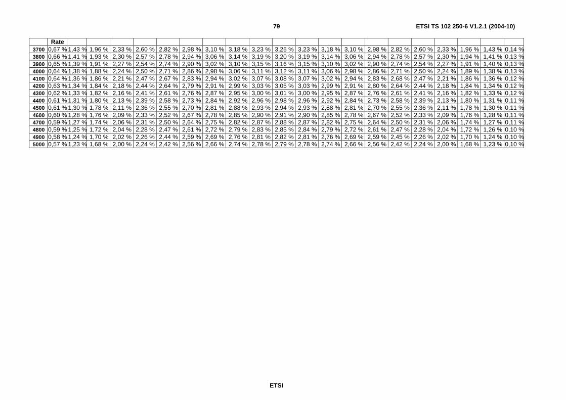
ETSI
ETSI TS 102 250-6 V1.2.1 (2004-10) 79
Rate 3700 0,67 % 1,43 % 1,96 % 2,33 % 2,60 % 2,82 % 2,98 % 3,10 % 3,18 % 3,23 % 3,25 % 3,23 % 3,18 % 3,10 % 2,98 % 2,82 % 2,60 % 2,33 % 1,96 % 1,43 % 0,14 %3800 0,66 % 1,41 % 1,93 % 2,30 % 2,57 % 2,78 % 2,94 % 3,06 % 3,14 % 3,19 % 3,20 % 3,19 % 3,14 % 3,06 % 2,94 % 2,78 % 2,57 % 2,30 % 1,94 % 1,41 % 0,13 %3900 0,65 % 1,39 % 1,91 % 2,27 % 2,54 % 2,74 % 2,90 % 3,02 % 3,10 % 3,15 % 3,16 % 3,15 % 3,10 % 3,02 % 2,90 % 2,74 % 2,54 % 2,27 % 1,91 % 1,40 % 0,13 %4000 0,64 % 1,38 % 1,88 % 2,24 % 2,50 % 2,71 % 2,86 % 2,98 % 3,06 % 3,11 % 3,12 % 3,11 % 3,06 % 2,98 % 2,86 % 2,71 % 2,50 % 2,24 % 1,89 % 1,38 % 0,13 %4100 0,64 % 1,36 % 1,86 % 2,21 % 2,47 % 2,67 % 2,83 % 2,94 % 3,02 % 3,07 % 3,08 % 3,07 % 3,02 % 2,94 % 2,83 % 2,68 % 2,47 % 2,21 % 1,86 % 1,36 % 0,12 %4200 0,63 % 1,34 % 1,84 % 2,18 % 2,44 % 2,64 % 2,79 % 2,91 % 2,99 % 3,03 % 3,05 % 3,03 % 2,99 % 2,91 % 2,80 % 2,64 % 2,44 % 2,18 % 1,84 % 1,34 % 0,12 %4300 0,62 % 1,33 % 1,82 % 2,16 % 2,41 % 2,61 % 2,76 % 2,87 % 2,95 % 3,00 % 3,01 % 3,00 % 2,95 % 2,87 % 2,76 % 2,61 % 2,41 % 2,16 % 1,82 % 1,33 % 0,12 %4400 0,61 % 1,31 % 1,80 % 2,13 % 2,39 % 2,58 % 2,73 % 2,84 % 2,92 % 2,96 % 2,98 % 2,96 % 2,92 % 2,84 % 2,73 % 2,58 % 2,39 % 2,13 % 1,80 % 1,31 % 0,11 %4500 0,61 % 1,30 % 1,78 % 2,11 % 2,36 % 2,55 % 2,70 % 2,81 % 2,88 % 2,93 % 2,94 % 2,93 % 2,88 % 2,81 % 2,70 % 2,55 % 2,36 % 2,11 % 1,78 % 1,30 % 0,11 %4600 0,60 % 1,28 % 1,76 % 2,09 % 2,33 % 2,52 % 2,67 % 2,78 % 2,85 % 2,90 % 2,91 % 2,90 % 2,85 % 2,78 % 2,67 % 2,52 % 2,33 % 2,09 % 1,76 % 1,28 % 0,11 %4700 0,59 % 1,27 % 1,74 % 2,06 % 2,31 % 2,50 % 2,64 % 2,75 % 2,82 % 2,87 % 2,88 % 2,87 % 2,82 % 2,75 % 2,64 % 2,50 % 2,31 % 2,06 % 1,74 % 1,27 % 0,11 %4800 0,59 % 1,25 % 1,72 % 2,04 % 2,28 % 2,47 % 2,61 % 2,72 % 2,79 % 2,83 % 2,85 % 2,84 % 2,79 % 2,72 % 2,61 % 2,47 % 2,28 % 2,04 % 1,72 % 1,26 % 0,10 %4900 0,58 % 1,24 % 1,70 % 2,02 % 2,26 % 2,44 % 2,59 % 2,69 % 2,76 % 2,81 % 2,82 % 2,81 % 2,76 % 2,69 % 2,59 % 2,45 % 2,26 % 2,02 % 1,70 % 1,24 % 0,10 %5000 0,57 % 1,23 % 1,68 % 2,00 % 2,24 % 2,42 % 2,56 % 2,66 % 2,74 % 2,78 % 2,79 % 2,78 % 2,74 % 2,66 % 2,56 % 2,42 % 2,24 % 2,00 % 1,68 % 1,23 % 0,10 %
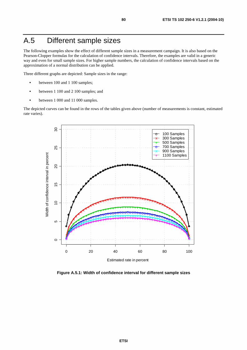
ETSI
ETSI TS 102 250-6 V1.2.1 (2004-10) 80
A.5 Different sample sizes The following examples show the effect of different sample sizes in a measurement campaign. It is also based on the Pearson-Clopper formulas for the calculation of confidence intervals. Therefore, the examples are valid in a generic way and even for small sample sizes. For higher sample numbers, the calculation of confidence intervals based on the approximation of a normal distribution can be applied.
Three different graphs are depicted: Sample sizes in the range:
• between 100 and 1 100 samples;
• between 1 100 and 2 100 samples; and
• between 1 000 and 11 000 samples.
The depicted curves can be found in the rows of the tables given above (number of measurements is constant, estimated rate varies).
0 20 40 60 80 100
05
1015
2025
30
Estimated rate in percent
Wid
th o
f con
fiden
ce in
terv
al in
per
cent
x
xx
xx
xxx xxxx xxx xxx xxx xxx xxx xxx xxx xxx xxx xxxx xxxx
xx
x
x+
++
++++++++++++++++++++++++++++++++++++++++++++++
+
+o
oo
oooooooooooooooooooooooooooooooooooooooooooooo
o
ox
xxxx xxx xxxx xxx xxx xxx xxx xxx xxx xxx xxx xxx xxxx xxx xxx
x
x++
++++++++++++++++++++++++++++++++++++++++++++++++
+
ox+ox+
100 Samples300 Samples500 Samples700 Samples900 Samples1100 Samples
Figure A.5.1: Width of confidence interval for different sample sizes
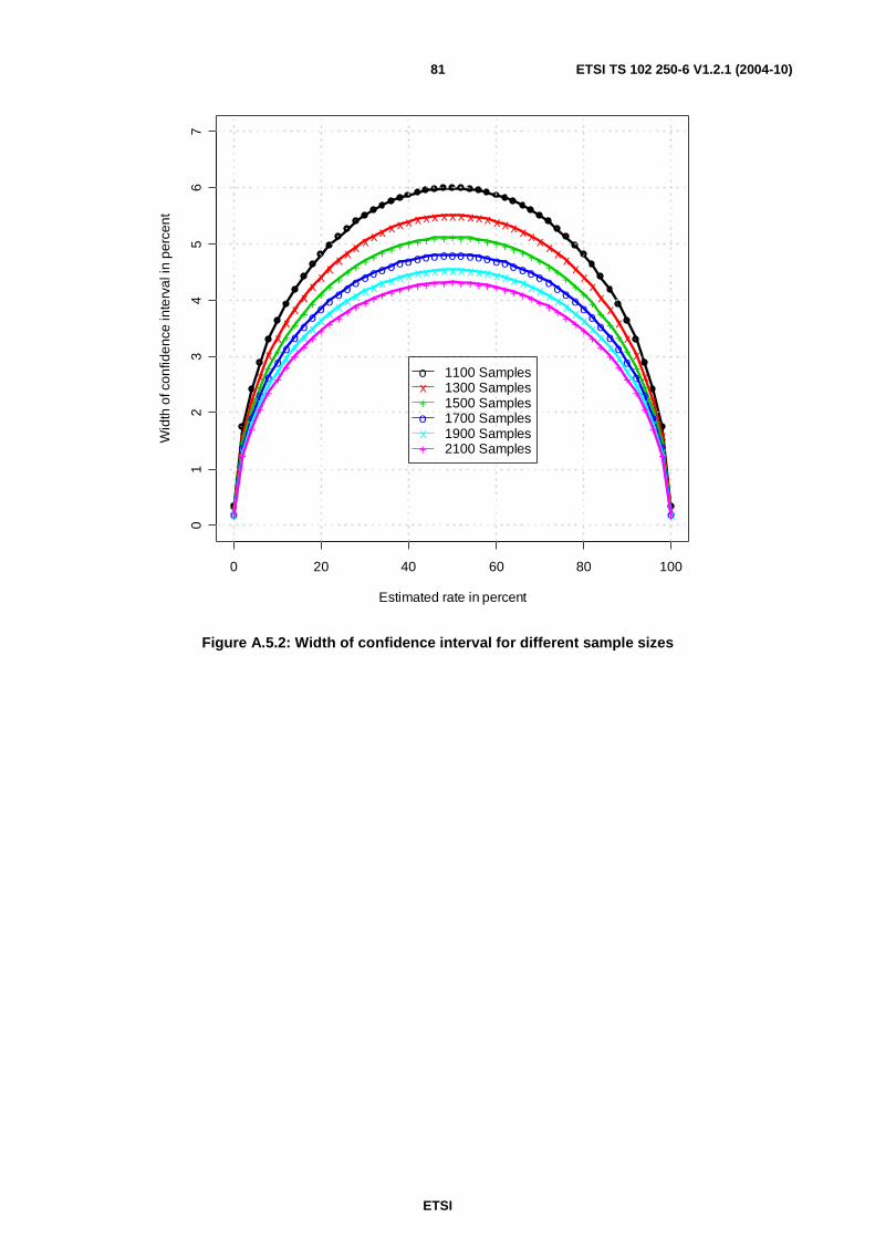
ETSI
ETSI TS 102 250-6 V1.2.1 (2004-10) 81
0 20 40 60 80 100
01
23
45
67
Estimated rate in percent
Wid
th o
f con
fiden
ce in
terv
al in
per
cent
x
x
x
x
xx
xx
xx
xx
xxx xxx xxx xxx xxx xxx xxx xxx xxxx
xx
xx
xx
x
x
x
x
x+
+
+
++
++
++
++++++++++++++++++++++++++++++++
++
++
++
+
+
+
+o
o
o
oo
oo
oo
oooooooooooooooooooooooooooooooo
oo
oo
oo
o
o
o
ox
x
x
xx
xx
xx
xxx xxx xxx xxx xxx xxx xxx xxx xxx xxx xx
xx
xx
xx
x
x
x
x+
+
+
++
++
++
++++++++++++++++++++++++++++++++++
++
++
+
+
+
+
ox+ox+
1100 Samples1300 Samples1500 Samples1700 Samples1900 Samples2100 Samples
Figure A.5.2: Width of confidence interval for different sample sizes
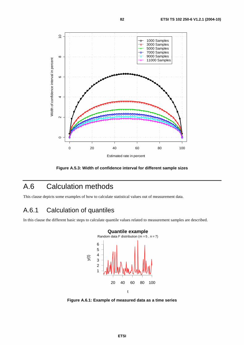
ETSI
ETSI TS 102 250-6 V1.2.1 (2004-10) 82
0 20 40 60 80 100
02
46
810
Estimated rate in percent
Wid
th o
f con
fiden
ce in
terv
al in
per
cent
x
xx
xx xxx xxxx xxx xxx xxx xxx xxx xxx xxx xxx xxx xxxx xxx x
xx
x
x+
++
++++++++++++++++++++++++++++++++++++++++++++++
+
+0
000000000000000000000000000000000000000000000000
0
0x
xxxx xxx xxxx xxx xxx xxx xxx xxx xxx xxx xxx xxx xxxx xxx xxx
x
x+
+++++++++++++++++++++++++++++++++++++++++++++++++
+
ox+ox+
1000 Samples3000 Samples5000 Samples7000 Samples9000 Samples11000 Samples
Figure A.5.3: Width of confidence interval for different sample sizes
A.6 Calculation methods This clause depicts some examples of how to calculate statistical values out of measurement data.
A.6.1 Calculation of quantiles In this clause the different basic steps to calculate quantile values related to measurement samples are described.
Quantile example
t
y(t)
Random data F distribution (m = 5 , n = 7)
20 40 60 80 100
123456
Figure A.6.1: Example of measured data as a time series
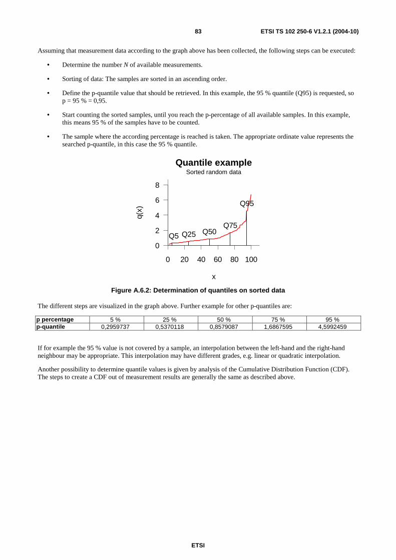
ETSI
ETSI TS 102 250-6 V1.2.1 (2004-10) 83
Assuming that measurement data according to the graph above has been collected, the following steps can be executed:
• Determine the number N of available measurements.
• Sorting of data: The samples are sorted in an ascending order.
• Define the p-quantile value that should be retrieved. In this example, the 95 % quantile (Q95) is requested, so p = 95 % = 0,95.
• Start counting the sorted samples, until you reach the p-percentage of all available samples. In this example, this means 95 % of the samples have to be counted.
• The sample where the according percentage is reached is taken. The appropriate ordinate value represents the searched p-quantile, in this case the 95 % quantile.
Quantile example
x
q(x)
Sorted random data
0 20 40 60 80 100
0
2
4
6
8
Q5 Q25 Q50Q75
Q95
Figure A.6.2: Determination of quantiles on sorted data
The different steps are visualized in the graph above. Further example for other p-quantiles are:
p percentage 5 % 25 % 50 % 75 % 95 % p-quantile 0,2959737 0,5370118 0,8579087 1,6867595 4,5992459
If for example the 95 % value is not covered by a sample, an interpolation between the left-hand and the right-hand neighbour may be appropriate. This interpolation may have different grades, e.g. linear or quadratic interpolation.
Another possibility to determine quantile values is given by analysis of the Cumulative Distribution Function (CDF). The steps to create a CDF out of measurement results are generally the same as described above.

ETSI
ETSI TS 102 250-6 V1.2.1 (2004-10) 84
A.7 Reporting of results This clause describes which pieces of information should be given to the reader when generating a test report. The categories of different data types are related to the definitions in clause 4.
A.7.1 Methods to use The variables x, y and z in the following table must be accordingly replaced by the estimated data.
When quantile values are used, it should be kept in mind that the computation of quantiles separates a low percentage of outlier data from the remaining data. This means:
• If lower values represent a better outcome from the customer's perspective, a small percentage containing the highest values could be separated by calculating a 95 %-quantile or a 90 %-quantile. This is the case for example for duration values.
• If higher values represent a better outcome from the customer's perspective, a small percentage containing the lowest values could be separated by calculating a 5 %-quantile or a 10 %-quantile. This is the case for example for throughput values.
• Related to content quality, the appropriate quantile computation orientates itself on the scale of the determined test results. In practice, some algorithms define a value of 0 on a scale from 0 to 5 as the best quality whereas others define the value of 5 as the highest possible quality. The table below gives some hints how to use the quantile computation in these cases.
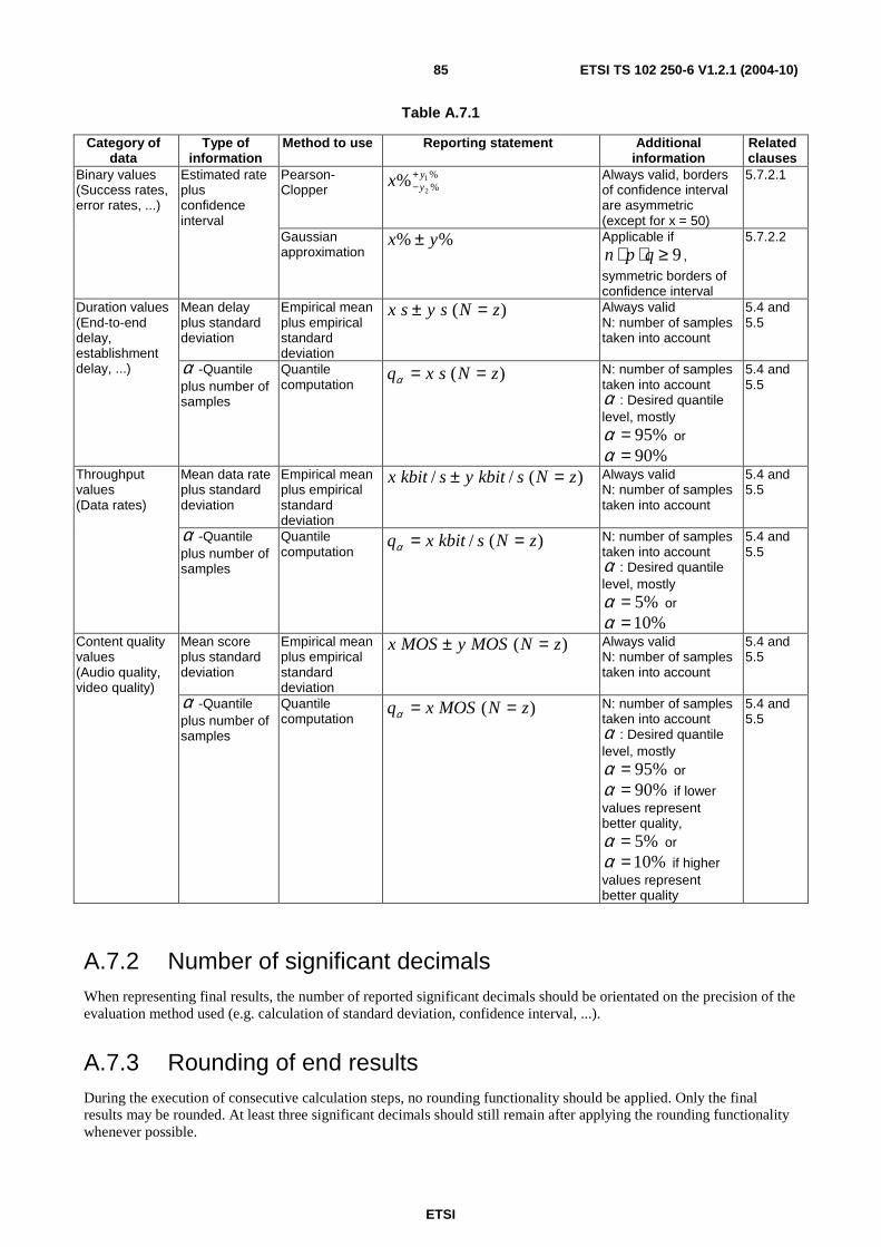
ETSI
ETSI TS 102 250-6 V1.2.1 (2004-10) 85
Table A.7.1
Category of data
Type of information
Method to use Reporting statement Additional information
Related clauses
Pearson-Clopper
%%
1
2% y
yx +− Always valid, borders
of confidence interval are asymmetric (except for x = 50)
5.7.2.1 Binary values (Success rates, error rates, ...)
Estimated rate plus confidence interval
Gaussian approximation
%% yx ± Applicable if 9≥⋅⋅ qpn ,
symmetric borders of confidence interval
5.7.2.2
Mean delay plus standard deviation
Empirical mean plus empirical standard deviation
)( zNsysx =± Always valid N: number of samples taken into account
5.4 and 5.5
Duration values (End-to-end delay, establishment delay, ...) α -Quantile
plus number of samples
Quantile computation
)( zNsxq ==α N: number of samples taken into account α : Desired quantile level, mostly
%95=α or
%90=α
5.4 and 5.5
Mean data rate plus standard deviation
Empirical mean plus empirical standard deviation
)(// zNskbityskbitx =± Always valid N: number of samples taken into account
5.4 and 5.5
Throughput values (Data rates)
α -Quantile plus number of samples
Quantile computation
)(/ zNskbitxq ==α N: number of samples taken into account α : Desired quantile level, mostly
%5=α or
%10=α
5.4 and 5.5
Mean score plus standard deviation
Empirical mean plus empirical standard deviation
)( zNMOSyMOSx =± Always valid N: number of samples taken into account
5.4 and 5.5
Content quality values (Audio quality, video quality)
α -Quantile plus number of samples
Quantile computation
)( zNMOSxq ==α N: number of samples taken into account α : Desired quantile level, mostly
%95=α or
%90=α if lower values represent better quality,
%5=α or
%10=α if higher values represent better quality
5.4 and 5.5
A.7.2 Number of significant decimals When representing final results, the number of reported significant decimals should be orientated on the precision of the evaluation method used (e.g. calculation of standard deviation, confidence interval, ...).
A.7.3 Rounding of end results During the execution of consecutive calculation steps, no rounding functionality should be applied. Only the final results may be rounded. At least three significant decimals should still remain after applying the rounding functionality whenever possible.

ETSI
ETSI TS 102 250-6 V1.2.1 (2004-10) 86
Annex B (informative): Bibliography
[BAT] Bates, D.M. and Chambers, J.M: "Nonlinear regression Analysis and Applications", Wiley & Sons, 1988.
[BRO] I.N. Bronstein, K.A. Semendjajew, G. Musiol, H. Mühlig: "Handbook of Mathematics", Verlag Harri Deutsch; Frankfurt/Main, 1999.
[BOX] Box, Cox: "An analysis of transformations", Journal of the Royal Statistical Society, vol. B 26, p. 211-251, 1964.
[E.800] Terms and Definitions Related to Quality of Service and Network Performance including Dependability, ITU-T Recommendation (1994).
[HARD] W.C. Hardy: "QoS Measurement and Evaluation of Telecommunications Quality of Service", Wiley & Sons, 2001.
[HART] J. Hartung: "Lehr- und Handbuch der angewandten Statistik", Oldenbourg Wissenschaftsverlag, 13th meditation, 2002.
[LAW] A. M. Law, W. D. Kelton: "Simulation modeling and analysis", McGraw-Hill, 3rd edition, 2000.
[MOOD] Mood, Graybill, Boes: "Introduction to the theory of statistics", McCraw-Hill Statistics Series, 1974.
[VEN] Venables, W.N. and Ripley, B.D.: "Modern Applied Statistics with S-Plus", Springer Verlag, 1999.

ETSI
ETSI TS 102 250-6 V1.2.1 (2004-10) 87
History
Document history
V1.1.1 May 2004 Publication
V1.2.1 October 2004 Publication