Post-glacial vegetation dynamics:Bayesian inference for tree abundances

using the fossil pollen record

Chris PaciorekDepartment of Biostatistics

Harvard School of Public Health

Jason McLachlanCenter for Population Biology

UC-Davis

September 16, 2005

www.biostat.harvard.edu/~paciorek

LYX - FoilTEX - pdfLATEX

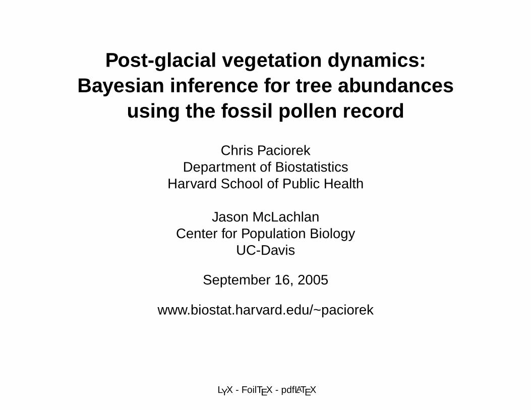
Scientific Setting

Trees release pollen that accumulates in lake sediments over time.

Ecologists use fossil pollen data collected from lake sediment coresand identified to genus to assess tree species abundances over time.

The pollen record is a biased, noisy reflection of the true tree veg-etation.

Current analysis methods focus on time series plots of individualpond records.

A spatio-temporal model can help to estimate spatial maps of treespecies compositions at multiple time points over several millenia byunderstanding the relationship between the pollen record and vegeta-tion.

The model needs at least one time point of concurrent pollenand ground-truth vegetation data to estimate the relationship betweenpollen and actual vegetation.

1

Central New England pollen and vegetation data

600000 700000 8000004600

000

4700

000

4800

000

Colonial era

600000 700000 8000004600

000

4700

000

4800

000

Modern era

600000 700000 8000004600

000

4700

000

4800

000

600000 700000 8000004600

000

4700

000

4800

000

beech

birch

chestnut

hemlock

hickory

maple

oak

pine

spruce

other

Figure 1: Colonial era witness tree data (top left) and modern plot data(top right); colonial (bottom left) and modern (bottom right) pollen data

2

Goals

• Understand the spatial relationship between pollen and vegetation.At what resolution do ponds predict vegetation? How far and inwhat quantity does pollen disperse?

• Estimate and compare spatial patterns in tree abundances for thecolonial and modern eras based on relevant vegetation data.

• Predict spatial patterns in tree abundances based on pollen dataover the past few thousand years, with uncertainty estimates.

• Assess the predictions to understand tree community dynamics:changing abundance and ranges of tree taxa over time.

• Assess the degree of certainty reasonable in making inferenceabout tree abundances based on pollen records. At what spatialscale can the pollen record distinguish spatial heterogeneity in treeabundances?

• Use the model to integrate genetic data and understand geneticheterogeneity.

3

4

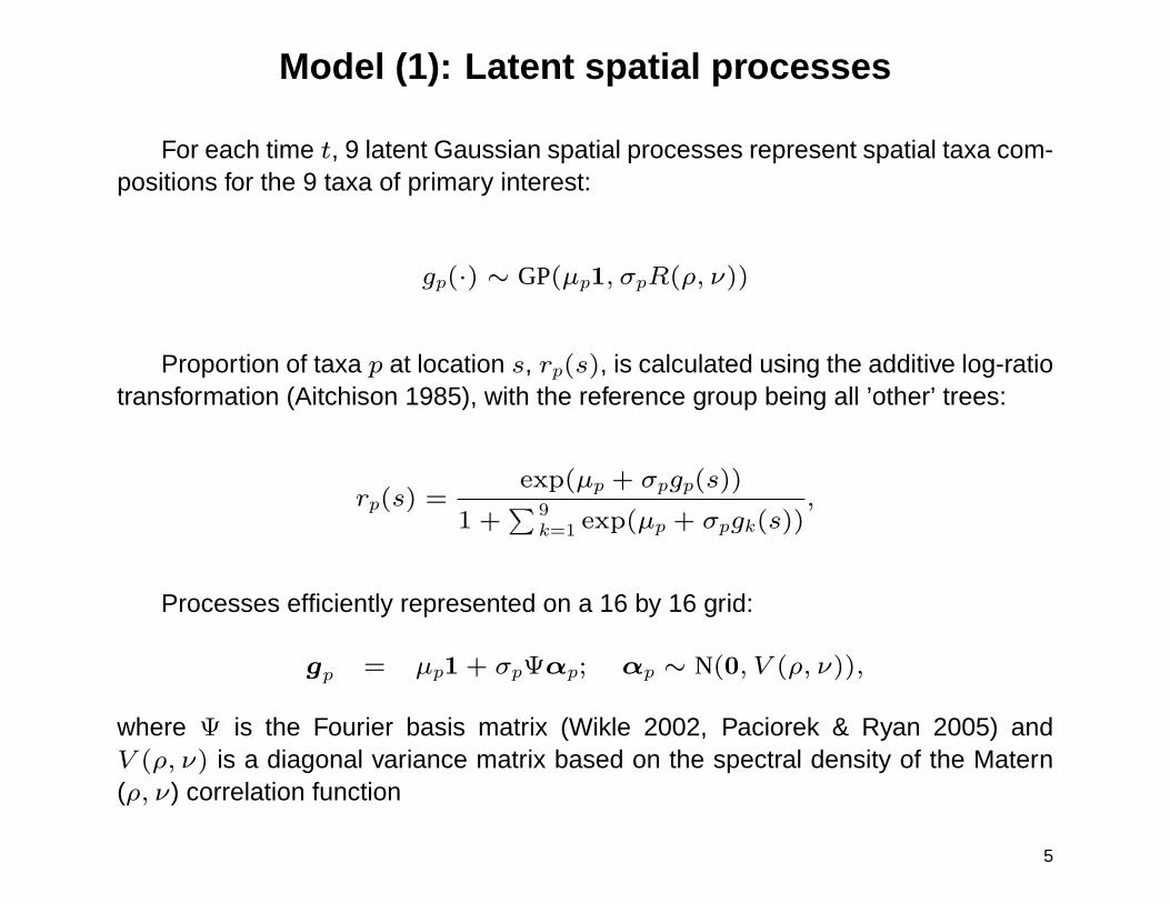
Model (1): Latent spatial processes

For each time t, 9 latent Gaussian spatial processes represent spatial taxa com-positions for the 9 taxa of primary interest:

gp(·) ∼ GP(µp1, σpR(ρ, ν))

Proportion of taxa p at location s, rp(s), is calculated using the additive log-ratiotransformation (Aitchison 1985), with the reference group being all ’other’ trees:

rp(s) =exp(µp + σpgp(s))

1 +∑9

k=1 exp(µp + σpgk(s)),

Processes efficiently represented on a 16 by 16 grid:

gp = µp1 + σpΨαp; αp ∼ N(0, V (ρ, ν)),

where Ψ is the Fourier basis matrix (Wikle 2002, Paciorek & Ryan 2005) andV (ρ, ν) is a diagonal variance matrix based on the spectral density of the Matern(ρ, ν) correlation function

5

Model (2): Likelihood terms

• Modern plot data (tree counts), s = 1, . . . , 1161:

– fs ∼ Dir-multi(nf,s, αtr(s))

– αf is extra-multinomial heterogeneityr(s) is composition vector (r1(s), . . . , r10(s))

• Colonial surveys (witness tree counts in townships), s = 1, . . . , 183:

– ws ∼ Dir-multi(nw,s, αwr(s))– r(s) is the weighted composition based on town-gridbox overlap

• Pollen data (pollen grain counts from 22 ponds at a fixed time),s = 1, . . . , 22:

– cs ∼ Dir-multi(nc,s, αcφ · r(s))– φ scales compositions to account for taxa heterogeneity in pollen

production and dispersal (element-wise multiplication)

6

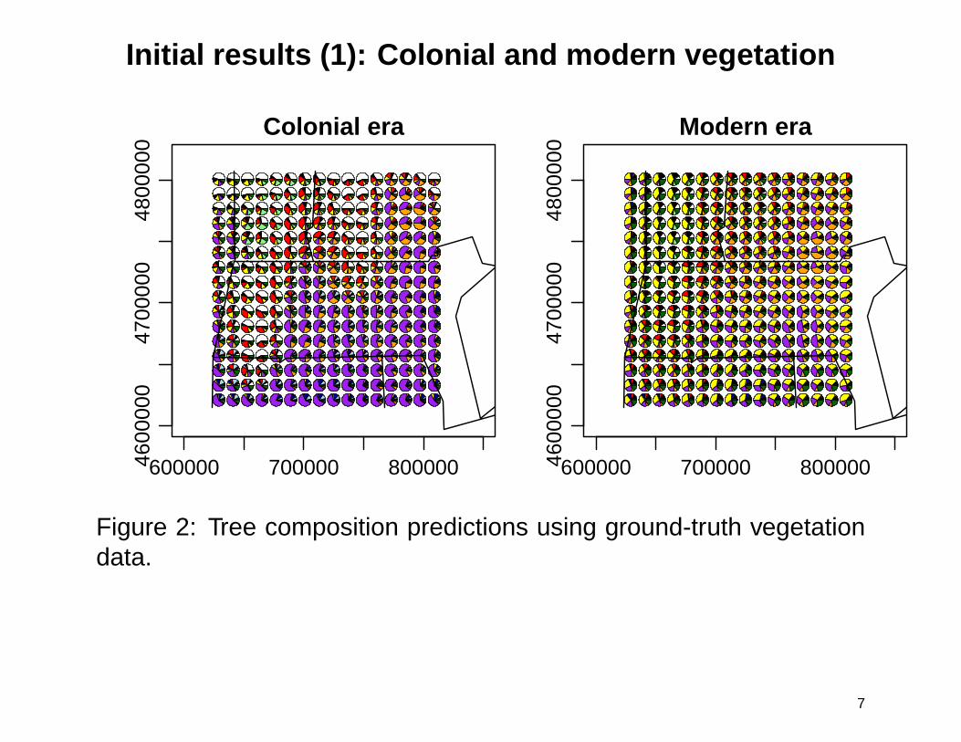
Initial results (1): Colonial and modern vegetation

600000 700000 8000004600

000

4700

000

4800

000

Colonial era

600000 700000 8000004600

000

4700

000

4800

000

Modern era

Figure 2: Tree composition predictions using ground-truth vegetationdata.

7

Initial results (2): Predictions based on pollen

600000 700000 8000004600

000

4700

000

4800

000

Colonial era

600000 700000 8000004600

000

4700

000

4800

000

Modern era

Figure 3: Tree composition predictions using only pollen data.

8

Pollen-vegetation mismatch

beec

hbi

rch

ches

tnut

hem

lock

hick

ory

map

leoa

kpi

nesp

ruce

othe

r

polle

n pr

oduc

tion

0.0

0.1

0.2

0.3

0.4 colonial era

beec

hbi

rch

ches

tnut

hem

lock

hick

ory

map

leoa

kpi

nesp

ruce

othe

r0.0

0.1

0.2

0.3

0.4 modern era

φ parameters (see left) adjust for differential pollen pro-

duction and dispersal, but even after adjusting for φ̂, we

see more homogeneity in the pollen data than in the

smoothed ground-truth vegetation. This appears to make

it difficult to infer vegetation from pollen, based on di-

agnostic plots for the colonial era comparing vegetation

composition to pollen composition, by pond (below left)

and by taxa (below right).

●

●●

●

●●

●

●

●●

0.0 0.2

0.0

0.3

predicted veg

phi−

adju

sted

pol

len pond 1

●

●●

●

●

●

●

●

●

●

0.05 0.20

0.05

0.25

predicted veg

phi−

adju

sted

pol

len pond 3

●● ●

●●●

●

●

●

●

0.0 0.2 0.4

0.0

0.4

predicted veg

phi−

adju

sted

pol

len pond 4

●

●●●●●

●

●

●●

0.0 0.2 0.4

0.0

0.4

predicted veg

phi−

adju

sted

pol

len pond 5

●

●●

●●

●

●

●

●●

0.0 0.2 0.40.

00.

3

predicted veg

phi−

adju

sted

pol

len pond 6

●

●●

●

● ●

●

●

●

●

0.0 0.2 0.4 0.6

0.0

0.4

predicted veg

phi−

adju

sted

pol

len pond 7

●

●

●

●●

●

●

●

●

●

0.0 0.2 0.4

0.0

0.3

predicted veg

phi−

adju

sted

pol

len pond 8

●

●●

●

●

●

●

●

●

●

0.00 0.15 0.30

0.00

0.20

predicted veg

phi−

adju

sted

pol

len pond 9

●●●● ●●

●

●●●

0.0 0.3 0.6

0.0

0.4

predicted veg

phi−

adju

sted

pol

len pond 10

●●●

●

●●

●

●

●●

0.0 0.2 0.4

0.0

0.3

predicted veg

phi−

adju

sted

pol

len pond 11

●

●●

●

●

●

●

●

●●

0.00 0.10 0.20

0.00

0.20

predicted veg

phi−

adju

sted

pol

len pond 12

●

●

● ●

●●

●●

●

●

0.00 0.15 0.30

0.00

0.20

predicted veg

phi−

adju

sted

pol

len pond 13

●

●

●

●

●

●●

●●

●

0.0 0.2 0.4

0.0

0.3

predicted veg

phi−

adju

sted

pol

len pond 14

●

●●

●

●●

●

●

●

●

0.00 0.15 0.30

0.00

0.25

predicted veg

phi−

adju

sted

pol

len pond 15

●

●

●

●

●

●

●

●

●

●

0.0 0.2

0.0

0.3

predicted veg

phi−

adju

sted

pol

len pond 16

●● ●

● ●●

●

●

●●

0.0 0.2 0.4

0.0

0.3

predicted veg

phi−

adju

sted

pol

len pond 17

●

●●

●

●

●

●●

●●

0.00 0.10 0.20

0.00

0.20

predicted veg

phi−

adju

sted

pol

len pond 18

●

● ●●

●●

●

●

●

●

0.00 0.15 0.30

0.00

0.20

predicted veg

phi−

adju

sted

pol

len pond 19

●

●●

●

●

●

● ●

●●

0.00 0.15

0.00

0.20

predicted veg

phi−

adju

sted

pol

len pond 20

●●●

●●●

●

●●

●

0.0 0.3 0.6

0.0

0.4

predicted veg

phi−

adju

sted

pol

len pond 21

●●●

●●●

●

●

●●

0.0 0.3 0.6

0.0

0.4

predicted veg

phi−

adju

sted

pol

len pond 22

●

●

●●

●●

●

●

●

●

0.0 0.2

0.0

0.2

predicted veg

phi−

adju

sted

pol

len pond 23

●●

●●●

●●

●

●●

●

●

●

●

●

●

●●

●

●●

●

0.0 0.2 0.4 0.6

0.0

0.2

0.4

0.6

predicted veg

phi−

adju

sted

pol

len

beech

●

●

●

●●

●

●

●

● ●

●

●

●

●

●

●

●

●

●

●●

●

0.02 0.06

0.02

0.06

predicted veg

phi−

adju

sted

pol

len

birch

●

●

●●

●

●

●

●● ●

●

●

●

●

●

●

●

●

●●●

●

0.00 0.05 0.10 0.15

0.00

0.05

0.10

0.15

predicted veg

phi−

adju

sted

pol

len

chestnut

●

●●

● ●

●

●

●

●

●

●

●

●●

●

●

●

●

●

●●

●

0.00 0.10 0.20 0.30

0.00

0.10

0.20

0.30

predicted veg

phi−

adju

sted

pol

len

hemlock

●●

●

●

●

● ●●

●

●●●● ●

●

●

●

●●

●

●

●

0.00 0.04 0.08

0.00

0.04

0.08

predicted veg

phi−

adju

sted

pol

len

hickory

●

●

● ●

●

●

●

●

●●

●

●

●

●

●

●

●

●

●

●●●

0.05 0.15

0.05

0.15

predicted veg

phi−

adju

sted

pol

len

maple

●

●

●●

●●

●

●

●

●

●

●●

●

●

●

●

●●

●●

●

0.0 0.2 0.4 0.6

0.0

0.2

0.4

0.6

predicted veg

phi−

adju

sted

pol

len

oak

●

●●

●

●

●

●

●

●

●

●●

●

●

●

●

●

●

●

●

●●

0.00 0.10 0.20 0.30

0.00

0.10

0.20

0.30

predicted veg

phi−

adju

sted

pol

len

pine

●

●

●

●

●

●●●

●

●

●

●

●

● ●●

●

●

●

●

●

●

0.00 0.02 0.04

0.00

0.02

0.04

predicted veg

phi−

adju

sted

pol

len

spruce

●

●

●

●

●

●

●

●

●

●

●

●●

●●

●

●

●

●

●

●

●

0.04 0.08 0.12

0.04

0.08

0.12

predicted veg

phi−

adju

sted

pol

len

other

9

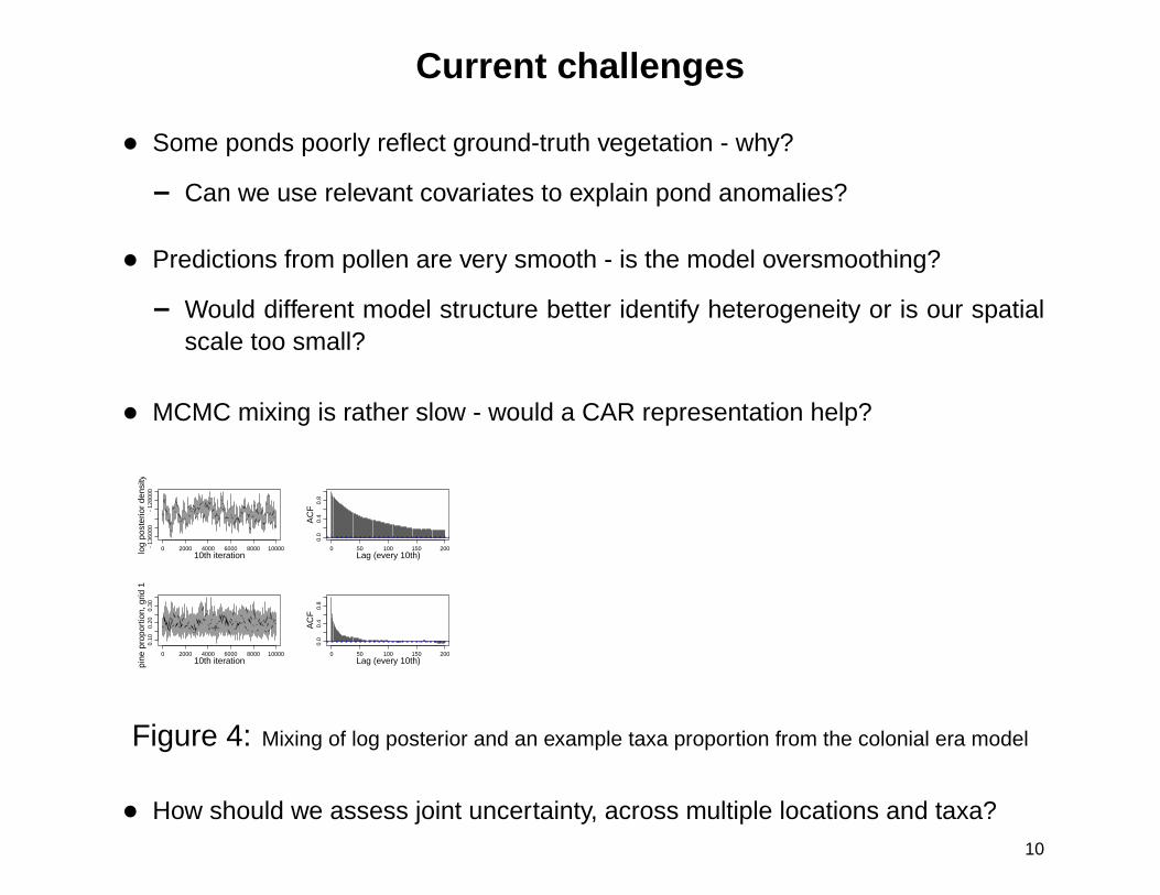
Current challenges

• Some ponds poorly reflect ground-truth vegetation - why?

– Can we use relevant covariates to explain pond anomalies?

• Predictions from pollen are very smooth - is the model oversmoothing?

– Would different model structure better identify heterogeneity or is our spatialscale too small?

• MCMC mixing is rather slow - would a CAR representation help?

0 2000 4000 6000 8000 10000−13

6000

−12

8000

10th iterationlog

post

erio

r de

nsity

0 50 100 150 200

0.0

0.4

0.8

Lag (every 10th)

AC

F

0 2000 4000 6000 8000 10000

0.10

0.20

0.30

10th iterationpine

pro

port

ion,

grid

136

0 50 100 150 200

0.0

0.4

0.8

Lag (every 10th)

AC

F

Series rStore[136, 8, which]

Figure 4: Mixing of log posterior and an example taxa proportion from the colonial era model

• How should we assess joint uncertainty, across multiple locations and taxa?10

Future work

• Continued model exploration and selection

• Addition of ponds from north (NH/VT) and south (CT) parts of studyregion to assess ability of pollen to resolve spatial variability

• Predictive inference over the past 4000 years, including modellingtemporal autocorrelation in the latent processes if necessary

• More explicit pollen dispersal modelling, perhaps with a long-distance component

• Expansion to the northeastern United States + southeasternCanada to get to a scale where pollen can resolve spatial hetero-geneity and assess tree migration

• Integration of the modelling with genetic data to better understandmigration and genetic heterogeneity

11