Embed Size (px)
Citation preview
General rights Copyright and moral rights for the publications made accessible in the public portal are retained by the authors and/or other copyright owners and it is a condition of accessing publications that users recognise and abide by the legal requirements associated with these rights.
Users may download and print one copy of any publication from the public portal for the purpose of private study or research.
You may not further distribute the material or use it for any profit-making activity or commercial gain
You may freely distribute the URL identifying the publication in the public portal If you believe that this document breaches copyright please contact us providing details, and we will remove access to the work immediately and investigate your claim.
Downloaded from orbit.dtu.dk on: Jun 03, 2020
Post-Combustion Capture of CO2 from Fossil Fueled Power Plants
Faramarzi, Leila
Publication date:2010
Document VersionPublisher's PDF, also known as Version of record
Link back to DTU Orbit
Citation (APA):Faramarzi, L. (2010). Post-Combustion Capture of CO2 from Fossil Fueled Power Plants. Technical Universityof Denmark.
PPoosstt--CCoommbbuussttiioonn CCaappttuurree ooff CCOO22 ffrroomm FFoossssiill FFuueelleedd
PPoowweerr PPllaannttss
by
Leila Faramarzi
PhD Thesis
April 2010
Center for Energy Resources Engineering
Department of Chemical and Biochemical Engineering
Technical University of Denmark
DK-2800 Kongens Lyngby, Denmark
ii
Summary
Almost one third of the atmospheric CO2 accumulation resulting from anthropogenic activities is due to the electric power production. CO2 capture, transport and storage (CCS) from fossil fueled power plants is thus gaining growing attention as an opportunity to reduce greenhouse gas emission. CCS is particularly a promising option as there is no need to change the energy supply infrastructure and to make large changes to the basic process of power generation. The alkanolamine-based post-combustion capture (PCC) process is considered the state of art technology for CO2 removal from flue gases. Alkanolamine processes are applicable at low concentrations of CO2 and that makes them favorable for flue gas cleaning.
In this project it was intended to apply an advanced thermodynamic tool for the description of the phase equilibria of CO2-alkanolamines-H2O systems over a wide range of temperature, partial pressure of CO2 and alkanolamine strength.
Experimental data on the solubility of CO2 in alkanolamine solutions are imperative for the thermodynamic modeling and design of PCC units. Therefore, before the thermodynamic modeling stage the open literature vapor-liquid equilibrium (VLE) data of aqueous mixtures of CO2 in single and blended alkanolamines were widely investigated and a comprehensive database also including other thermodynamic properties of such systems is established. This includes solubility of CO2 in monoethanolamine (MEA), diethanolamine (DEA), N-methyldiethanolamine (MDEA), diglaycolamine (DGA), 2-amino-2-hydroxymethyl-1,3-propandiol (AHPD) and piperazine (PZ). The developed database covers a wide range of temperature, acid gas partial pressure and alkanolamine concentration. The data of MEA, MDEA and MEA+MDEA systems were used for modeling.
The thermodynamic model, extended UNIQUAC, was used to calculate both physical and chemical equilibria of the single amine systems MEA and MDEA. Moreover, the model was extended to a mixed alkanolamine system MEA+MDEA as amine-blends are considered a promising alternative for CO2 capture. It was aimed to keep the model to a rather limited number of adjustable parameters. The reason was that the existing advanced models are complex with large number of parameters while their predictive capability is far from ideal. In this work, only one set of adjustable parameters for correlation of different thermodynamic properties is used. Extended UNIQUAC has well represented the VLE of pure, binary (alkanolamine+water), ternary (CO2+alkanolamine+water), quaternary (CO2+mixed alkanolamines+water) systems, excess enthalpy, and freezing point depression of the alkanolamine+water systems. Also with a good accuracy, the model has predicted the speciation of the compounds in the aqueous phase. In addition, the formerly unavailable standard state properties of the alkanolamine ions MEA protonate, MEA carbamate and MDEA protonate are determined.
In the final stage of the project, the absorber column was modeled using MEA as absorbent. MEA, though coming with many drawbacks is considered a promising solvent at low partial pressures of CO2 as it reacts at a rapid rate. Furthermore, the cost of the raw material is low compared to that of secondary and tertiary amines.
To design the absorber column, a rate-based steady state model which was originally developed for the design of the CO2- 2-amino-2-methyl-propanol (AMP) absorber was adopted and improved for the design of the MEA absorber. Different mass transfer correlations were applied in the model and their influence on the model’s performance was investigated. The model’s predictions proved to be highly dependent on the mass transfer correlations applied.
iii
Analytical expressions for the calculation of the enhancement factor for the second order as well as the pseudo-first order reaction regime were integrated in the model and their impact on the model’s prediction was compared. The enhancement factor for the pseudo-first order reaction seemed to be not only sufficient, but the preferred approach for representing the experimental data for the loading ranges considered.
Different rate equations were integrated in the model. Overall, the applied equations for the kinetic rate yielded similar results.
The MEA absorber model has been successfully applied to CO2 absorber packed columns and validated against pilot plant data with good agreement.
Overall, the thermodynamic model and the simple model for the CO2 absorber packed column developed in this work are promising tools for simulating the capture process. If the developed models are included in the power plant simulation packages, they can provide powerful means for the design of the plants with integrated CO2 removal units.
iv
Resumé på dansk
Næsten en tredjedel af den CO2 udledning som kommer fra menneskeskabte aktiviteter skyldes produktion af elektrisk energi. Implementering af CO2 capture-teknologier, transport og lagring (CCS) i forbindelse med kulfyrede kraftværker er således ved at få voksende opmærksomhed som en mulighed for at reducere drivhusgasemissioner. CCS er især en lovende mulighed, da der ikke er behov for at ændre energiforsyningens infrastruktur eller foretage store ændringer i den grundlæggende proces for elproduktion. Den alkanolamine-baserede proces betragtes som den mest brugte teknologi for CO2 fjernelse fra røggassen blandt dem som kan bruges efter forbrænding (PCC). Alkanolamine processer kan bruges ved lave koncentrationer af CO2 og er derfor velegnede for røggasrensning.
I dette projekt er hensigten at anvende et avanceret termodynamisk værktøj til beskrivelse af faseligevægte af CO2-alkanolaminer-H2O systemer over en bred vifte af temperatur, CO2 partialtryk og alkanolamin koncentration.
Eksperimentelle data om opløselighed af CO2 i alkanolamin opløsninger er nødvendige for termodynamisk modellering og design af PCC enheder. Derfor blev en omfattende database med litteratur data først etableret.
Den termodynamiske model ”extended UNIQUAC” blev brugt til at beregne både fysiske og kemiske ligevægte for systemer med MEA og MDEA. Desuden blev der bestemt modelparametre for det blandede alkanolamin system MEA + MDEA. Model udviklingen sigtede efter at begrænse antallet af parametre. Årsagen var, at de eksisterende avancerede modeller er komplekse med mange parametre, mens deres evne til at beskrive termodynamiske egenskaber for den slags blandinger langt fra er optimal. I dette arbejde er kun ét sæt af parametre anvendt til at beskrive de forskellige termodynamiske egenskaber. Extended UNIQUAC kunne godt beskrive VLE af rene, binære (alkanolamine + vand), ternære (CO2 + alkanolamine + vand), og flere komponent (CO2 + blandede alkanolaminer + vand) systemer, exces enthalpi, og frysepunktsænkning af alkanolamin + vand systemer . Også med en god nøjagtighed, kan modellen forudsige speciering af stofferne i den vandige fase. De tidligere ukendte standard tilstand egenskaber for alkanolamine ioner protonate, MEA carbamat og MDEA protonate blev også bestemt i dette arbejde.
I den afsluttende fase af projektet blev absorptions kolonnen modelleret ved hjælp af MEA som absorbent. MEA, trods dens mange ulemper, betragtes som et lovende opløsningsmiddel med lav partialtryk af CO2 som medfører en hurtig reaktion. Desuden er omkostningerne til råvarer lave sammenlignet med sekundære og tertiære aminer.
Absorber design er baseret på en ”steady state” model, som oprindeligt blev udviklet for blandinger med 2-amino-2-methyl-propanol (AMP) absorber. Modellen blev videre udviklet og forbedret for anvendelse i MEA-baserede absorbere. Forskellige massetransport korrelationer blev anvendt i modellen og deres indflydelse på modellens resultater blev undersøgt. Modellens forudsigelser viste sig at være afhængig af hvilke massetransport korrelationer der anvendes. Analytisk udtryk for beregning af ”enhancement” faktor for anden orden samt for den pseudo-første ordens reaktioners regime blev integreret i modellen og deres påvirkning på modellens resultater blev sammenlignet. ”Enhancement” faktor for pseudo-første ordens reaktioner syntes at være tilstrækkeligt, og faktisk den foretrukne fremgangsmåde til at repræsentere de eksperimentelle data. MEA absorber modellen er anvendt med succes til CO2 absorbere udført som pakkede kolonner og valideret mod pilotanlæg data.

v
Resultaterne er tilfredstillende. Samlet set er den termodynamiske model og den simple model for CO2 absorber pakket kolonne udviklet under dette arbejde lovende værktøjer til at simulere processen.
vi
Preface
This work was accomplished at the Department of Chemical and Biochemical Engineering at the Technical University of Denmark (DTU) under the supervision of Professor Georgios M. Kontogeorgis, Associate Professor Kaj Thomsen and Professor Erling H. Stenby. The study started in February 2007 and ended in March 2010 and was financed by DTU, Dong Energy and Vattenfall.
Professor Georgios M. Kontogeorgis, chair of this PhD was keenly involved in this work, striking the outstanding balance between providing excellent guidelines and encouraging independence. Thank you for your valuable comments and suggestions and for urging me forward without which this work would not have come to fruition.
Thank you to my thesis co-advisor Associate Professor Kaj Thomsen for your exceptional guidance and for readily sharing your profound expertise on the subject matter in the most delightful manner. Your quest for performing high quality research was inspirational to me.
My deepest thanks and admiration go to Reader Michael L. Michelsen for the fruitful discussions we had which shed light on the path of this work. I benefited immensely from your counsel, comments and interest in this venture.
My gratitude to Professor Erling H. Stenby for giving me the chance to do a PhD at the Center for Energy Resources Engineering and for supporting me through some tough times I was through. Thank you for keeping the CO2 team in close contact with the industrial parties and thus making it possible for us to have a real world feeling of the matter.
Thank you to Victor Darde with whom countless discussions were had where ideas developed, and strengths and weaknesses of my arguments were gently identified. I never imagined that moving to our delightful CO2 office and having an officemate like you can be this much to my advantage.
Thank you to Philip Loldrup Fosbøl. Since you joined the CO2 Capture Project, you added a great momentum to our activities. Thank you for always being there with a brilliant answer to my questions. With you, getting stuck was history!
In keeping with the theme of this work, Jostein Gabrielsen was the one who introduced me to the world of CO2 capture. Thank you for openhandedly sharing your knowledge and data and moreover, paying a visit to the university whenever I needed your help.
To the one who has shown indefatigable support reminding me of my priorities in the face of hardships, I give credit to Ramin Moslemian. Thank you for being there for me as I followed this twisting path.
Finally, to Hassan on whose constant encouragement and love I have relied for many years. You have known no limits to my aspirations. Thank you for coming with me this far. Leila Faramarzi April 2010
vii
Table of Contents
Summary................................................................................................................................................................. ii
Resumé på dansk ................................................................................................................................................... iv
Preface ................................................................................................................................................................... vi
Chapter 1: General Introduction
1.1. Introduction ............................................................................................................................................... 2
1.2. Options for CO2 mitigation ........................................................................................................................ 2
1.3. Introduction to CO2 capture ....................................................................................................................... 3
1.3.1. Pre-combustion capture ................................................................................................................ 3
1.3.2. Oxy-fuel combustion .................................................................................................................... 4
1.3.3. Post-combustion capture .............................................................................................................. 5
1.3.3.1. Chemical solvents ...................................................................................................................................... 6
Amines .................................................................................................................................................................... 6
Aqueous ammonia .................................................................................................................................................. 8
1.4. R&D opportunities for CO2 capture by aqueous absorption...................................................................... 9
1.5. Thesis motivation and outline .................................................................................................................. 10
Phase 1: Thermodynamic Modeling ..................................................................................................................... 10
Phase 2: Modeling the Absorber ........................................................................................................................... 10
References ........................................................................................................................................................ 11
Chapter 2: Thermodynamic Modeling of Aqueous CO2+Alkanolamine Solutions
2.1. Introduction ............................................................................................................................................. 13
2.2. Chemical and phase equilibria ................................................................................................................. 14
2.2.1. Speciation equilibria .......................................................................................................................... 14
2.2.2. Vapor-liquid equilibria ............................................................................................................... 16
2.2.3. Pure component vapor pressure .................................................................................................. 17
2.3. Standard state properties .......................................................................................................................... 18
2.4. Model ...................................................................................................................................................... 19
2.4.1. Extended UNIQUAC ................................................................................................................. 21
2.5. Excess enthalpy ....................................................................................................................................... 23
2.6. Estimation of parameters ......................................................................................................................... 24
2.7. Parameter regression database ................................................................................................................. 24
2.7.1. Data of aqueous alkanolamine solutions (alkanolamine-water) ................................................. 26
2.7.2. Data on solubility of CO2 in single alkanolamines (CO2-alkanolamine-water VLE data) ......... 26
2.7.3. VLE measurement methods and associated errors ..................................................................... 28
2.7.4. Data on solubility of CO2 in mixed alkanolamines (CO2-amine blend-water VLE data) ........... 29
2.8. Results and discussion ............................................................................................................................. 29
2.8.1. Physical equilibrium ................................................................................................................... 32
MEA system ......................................................................................................................................................... 32
viii
MDEA system ...................................................................................................................................................... 36
MEA+MDEA system ........................................................................................................................................... 43
2.8.2. Chemical equilibrium ................................................................................................................. 45
2.9. Conclusions ............................................................................................................................................. 47
References ............................................................................................................................................................ 49
Chapter 3: Modeling the MEA Absorber
3.1. Introduction ............................................................................................................................................. 52
3.2. The chemistry of the aqueous CO2-MEA system .................................................................................... 52
3.3. Absorption model .................................................................................................................................... 53
3.3.1. Enhancement factor .................................................................................................................... 53
3.3.1.1. Modelling of mass transfer in liquid boundary layer: Physical mass transfer ................................ 54
3.3.1.2. Mass transfer with finite rate reaction............................................................................................. 55
Second order irreversible reactions....................................................................................................................... 55
Pseudo-first order reactions .................................................................................................................................. 58
3.3.2. Kinetics....................................................................................................................................... 59
3.3.3. Liquid-side mass transfer coefficient ......................................................................................... 60
3.3.4. Gas-side mass transfer coefficient .............................................................................................. 60
3.3.5. Effective interfacial area of packing ........................................................................................... 61
3.3.6. Physical properties ..................................................................................................................... 63
Density .................................................................................................................................................................. 63
Viscosity ............................................................................................................................................................... 63
Solubility .............................................................................................................................................................. 64
Diffusivity............................................................................................................................................................. 69
Surface tension ..................................................................................................................................................... 70
Heat capacity ........................................................................................................................................................ 71
3.3.7. Thermodynamics ........................................................................................................................ 72
3.4. Results and discussion ............................................................................................................................. 72
3.4.1. Pilot plant data used for simulation ............................................................................................ 72
3.4.2. Liquid-side mass transfer coefficient ......................................................................................... 73
3.4.3. Kinetic rate constant ................................................................................................................... 74
3.4.4. Effective packing interfacial area ............................................................................................... 74
3.4.5. Enhancement factor .................................................................................................................... 76
3.4.6. Enhanced volumetric liquid-side mass transfer coefficient ........................................................ 76
3.4.7. Total mass-transfer coefficient ................................................................................................... 77
3.4.8. Simulation results ....................................................................................................................... 77
3.5. Conclusions ............................................................................................................................................. 82
References ............................................................................................................................................................ 84
Chapter 4: Numerical Implementation of the Absorber Model
4.1. Material and energy balances in the packed column .............................................................................. 87

ix
References ............................................................................................................................................................ 90
Chapter 5: Conclusions and Future Prospect
5.1. Concluding remarks ................................................................................................................................. 92
5.1.1. On thermodynamic modelling using extended UNIQUAC model ................................................. 92
5.1.2. On modelling the MEA absorber .................................................................................................... 92
5.2. Challenges and future work ..................................................................................................................... 93
References ............................................................................................................................................................ 94
Appendix ............................................................................................................................................................. 95
Publications, key conference presentations and reports ................................................................................... 95


11
GENERAL INTRODUCTION
“The global warming scenario is pretty grim. I'm not sure I like the idea of polar bears
under a palm tree.”
Bjørn Lomborg, author of "The Skeptical Environmentalist."
Chapter 1
2
1.1. Introduction
The concentration of the atmospheric CO2 has risen 35% since the time of the industrial revolution. The current value of CO2 concentration in the atmosphere is 380 ppm. This increasing trend seems unlikely to slow down if no serious measure is taken to mitigate the anthropogenic sources. The Assessment Report of the Intergovernmental Panel on Climate Change (IPCC) estimated CO2 concentration to contribute to a global radiative forcing of 1.66 Wm-2, which is the greatest of all of the earth radiative components [1].
Global increase in energy demand together with a continued dependence on fossil fuel resources have significantly contributed to the increase in the atmospheric levels of CO2. International Energy Agency’s (IEA’s) World Energy Outlook 2007 [2] reports that the growth in energy demand will result in 57 percent energy related CO2 emissions by 2030. Although, in the current energy price situation, some argue that the global energy demand will be much lower than IEA forecast [3].
The largest anthropogenic emission sources in the globe are the fossil fueled power plants causing approximately one-third of the CO2 emissions. Coal-fired plants emit significantly more CO2 than natural gas plants. However coal is a very favorable energy source for power generation because it is relatively inexpensive compared to other fossil fuels [4].
Due to the apparent contribution of CO2 to the global warming, more lately there has been an emphasis on mitigating CO2 emission especially from the combustion processes associated with power generation. CO2 separation from gaseous streams has been practiced for decades. Much of the work concerned the separation of CO2 from methane for the purification of natural gas as many natural gas reservoirs contain significant amounts of acid gases like CO2.
1.2. Options for CO2 mitigation
Significant reductions in CO2 emissions from the global energy system can be feasible, using various combinations of low CO2 energy technologies.
The following main options can be considered for mitigating the emission of CO2 from fossil fuel emission sources:
1. Increasing the efficiency of fuel conversion 2. Switching to fuels which have lower carbon content 3. Using renewable energy where possible 4. Using nuclear energy 5. Separation and disposal of carbon dioxide
It is yet not clearly known to what extent different technologies for carbon emission mitigation will contribute to stabilization of the greenhouse gases concentration in the atmosphere. However, all the assessed scenarios concerning stabilization agree that 60 to 80% of the reductions over the course of the century would come from energy supply and use and, industrial mitigation processes. In many scenarios, energy efficiency plays a major role for most regions and time scales. For stabilization at lower carbon levels, scenarios put more emphasis on the use of low-carbon energy sources, such as renewable energy, nuclear power and the use of CO2 capture and storage [5].
General introduction
3
Although many existing coal fueled power plants suffer from low fuel conversion efficiency and rather high CO2 emissions, replacing them with new plants could have major economic impacts and there are chances of considerable political antagonism. The studies on the retirement of a few coal-fired power plants have shown that there is a large economic inducement for keeping the existing plants. These studies emphasize on the importance of retrofitting the available plants along with moving forward with capture options for new plants [6]. Though, it should be mentioned that retrofits have also drawbacks such as significant capacity and efficiency losses that require replacement capacity addition and increased consumption of fuel depending on the CO2 abatement technology. The 2009 Energy Information Administration (EIA) projection through 2030 shows only 2.3 GW of coal capacity retirements and 24.8 GW of new capacity, an overall net increase of 7% [7].
The diversity of energy supply can increase by renewable energy and over the long run renewable energy can at least partially replace dwindling fossil fuel resources. The use of renewable energy instead of fossil fuels can considerably reduce greenhouse gases and other pollutants. Some forms of renewable energy are now competitive in some market conditions. The main restriction in advancing renewable energy over the last few decades has been cost-effectiveness. The average costs of renewable energy, with the exception of large hydropower, biomass (for heat) and larger geothermal schemes are generally not competitive with fossil fuel prices. However, some renewable energy options for small-scale applications can now compete in the marketplace, including hot water from solar collectors [8].
The most promising method of mitigation considering the escalating global energy demand is post-combustion capture for existing fossil fuel plants followed by long-term, large-scale sequestration to deeply cut CO2 emissions.
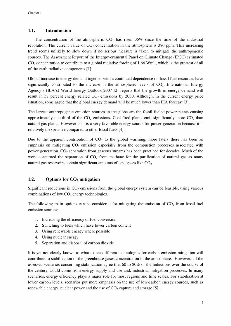
1.3. Introduction to CO2 capture
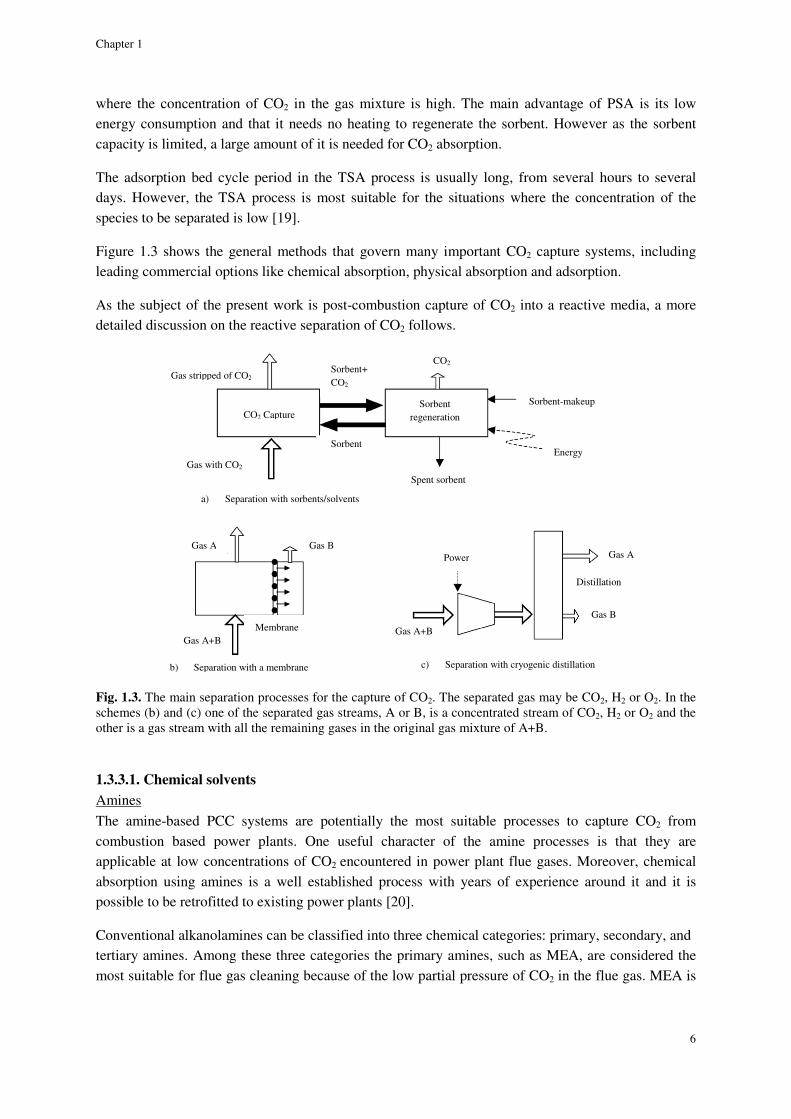
The CO2 capture methods to be combined with power generation are usually divided into three different groups: pre-combustion capture, oxyfuel combustion and post-combustion capture. Figure 1.1 shows a block diagram for these three methods.
1.3.1. Pre-combustion capture
Through reacting coal with steam and oxygen, fuel-bound carbon can first be converted to a form easy to capture. The products of this reaction which is called coal gasification are mainly carbon monoxide and hydrogen. This mixture is usually called synthesis gas or in short syngas.
Afterwards, two additional process units are required to capture CO2 from syngas. A shift reactor converts the carbon monoxide to CO2 through reaction with steam. Then, CO2 is separated from the H2-CO2 mixture. The CO2 is compressed for transport, while the H2 serves as a carbon-free fuel that is combusted to generate electricity in an Integrated Gasification Combined Cycle, IGCC. IGCC is a process in which a low-value fuel such as coal is converted to a high-hydrogen gas in a gasification process. The hydrogen is then used as the primary fuel for a gas turbine [9].
The high concentrations of CO2 and high operational pressures of the gasifiers make CO2 capture easier than the post-combustion capture process (PCC) though, the fuel conversion unit is costly compared to PCC. CO2 is removed using a chemical or a physical solvent such as selexol [10].
Chapter 1
4
As of the end of 2007, only four gigawatts IGCC power plants have been built worldwide, while both pre-combustion capture and IGCC technologies are considered to be available at present. The reason is, after the hydrogen is separated from the gas mixture, a gas turbine that can function in a hydrogen-rich environment is needed. Hydrogen-fired turbines are being developed for this purpose but yet are not in the technological state to be used in power plants [3].
Fig. 1.1 Power generation combined with three different methods for CO2 capture [1]
1.3.2. Oxy-fuel combustion
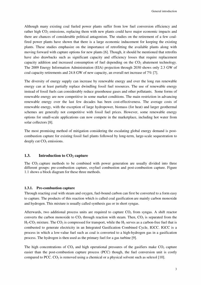
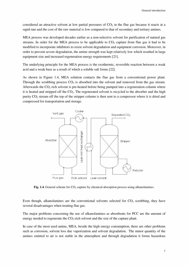
Rather than in air, pulverized coal oxy-fuel combustion burns fossil fuels in a mixture of recirculated flue gas (70-80% of the total flue gas) and oxygen (95% purity or higher). CO2-rich exhaust gas is recycled back to the boiler to control the combustion temperature. From the portion of the flue gas which is not recycled and is rich in carbon dioxide and water, water vapor can be condensed off and CO2 can be separated after cleaning the gas from the minor quantities of Ar, N2, NOx , SOx and other constituents from air leakage and fuel. The cleaned CO2 is then compressed and transported to storage or other suitable applications [11]. Oxy-combustion plants could enable relatively easy capture of CO2 at rates as high as 97%. Moreover NOx emissions will be drastically low in this technology. Production of oxygen is, however, very expensive and represents the largest cost in the CO2 capture process. Figure 1.2 shows how the sources of parasitic energy losses from a typical PCC plant compare to those from an oxy-combustion plant [6]. At present new technologies for the production of oxygen are being developed with lower energy consumption and lower cost of production [12].
Power & heat
CO2 separation
O2, N2,H2O
O2, N2,H2O
CO2, H2O
CO2 CO2
N2
H2
N2
N2
Post-combustion capture
Pre-combustion capture
Oxy-fuel combustion capture
Fuel Air Air
Fuel
Fuel
Air
Air
Flue gas
Power & heat
Power & heat
Air separation
Air separation
General introduction
5
Oxy-fuel combustion plants CO2 capture plants
Fig. 1.2. Parasitic energy losses for post-combustion capture and oxy-combustion Plants
1.3.3. Post-combustion capture
For PCC, the addition of capture and compression systems is necessary. The prominent PCC technologies also require the cleaning of the flue gas before the capture device. Removing the sulfur dioxide content of the flue gas as well as the particulate matter is particularly important as they cause corrosion and fouling in the system [13].
Several different approaches have been proposed for removing CO2 from flue gases on a large scale. The main approaches to the separation of CO2 from other light gases are: cryogenic distillation, membrane purification, absorption with liquids, and adsorption using solids.
Although cryogenic distillation is widely used for separation of other gases, it is not generally considered as a means for separation of CO2 from flue gases because the energy cost is very high.
Membrane technology has emerged to be a valuable option for separation of acidic gases due to its advantages such as economy, process safety and environmentally friendly nature. The application of membranes for CO2 separation from relatively concentrated sources has been extensively studied [14]. Membranes can be very efficiently used for separation especially when the components that are to pass through the membrane are present in a large concentration. For PCC, because CO2 is a minor component of the off-gases, membranes are not likely to be the most efficient approach for the separation. In contrast, for processes that involve relatively concentrated CO2 streams at elevated pressures, such as for pre-combustion capture, using membranes is a promising approach [15].
A well established process for separation of acid gases from gaseous streams is absorption by a liquid media. The liquid media are often aqueous alkanolamine (monoethanolamine, MEA, being the most widely known) solutions or other fluids with alkaline character, such as chilled or ambient temperature ammonia. The absorption in the liquid media takes place through chemical reaction of the acidic gases with the aqueous absorbent. Processes which are based on the application of physical solvents exist as well. Methanol [16] or poly-ethylene glycol [17] are two examples of physical absorbents.
Adsorption processes for gas separation via selective adsorption on solid media are also well-known. These adsorbents can operate via weak physical absorption processes or strong chemisorption interactions. Solid adsorbents such as zeolites or activated carbon are typically used in cyclic, multi-module processes of adsorption and desorption [18]. Desorption is induced by pressure swing absorption (PSA) or temperature swing absorption (TSA). The PSA process though is only applicable
59%10%
31%
Power for air separation
Power for pumps, fans, etc.
Power for carbon dioxide compressors
54%
8%
38%
Power loss from steam extraction
Power for pumps and fans for the capture processPower for carbon dioxide compressors
Chapter 1
6
where the concentration of CO2 in the gas mixture is high. The main advantage of PSA is its low energy consumption and that it needs no heating to regenerate the sorbent. However as the sorbent capacity is limited, a large amount of it is needed for CO2 absorption.
The adsorption bed cycle period in the TSA process is usually long, from several hours to several days. However, the TSA process is most suitable for the situations where the concentration of the species to be separated is low [19].
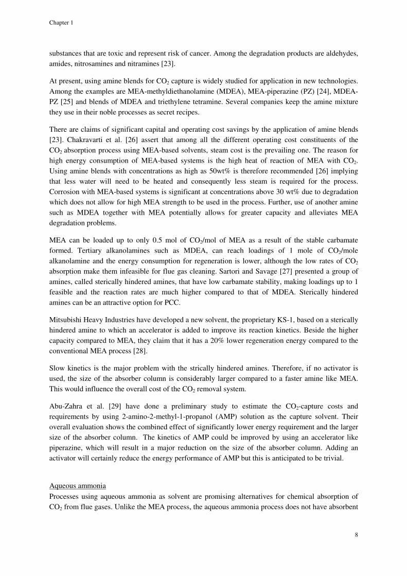
Figure 1.3 shows the general methods that govern many important CO2 capture systems, including leading commercial options like chemical absorption, physical absorption and adsorption.
As the subject of the present work is post-combustion capture of CO2 into a reactive media, a more detailed discussion on the reactive separation of CO2 follows.
Fig. 1.3. The main separation processes for the capture of CO2. The separated gas may be CO2, H2 or O2. In the schemes (b) and (c) one of the separated gas streams, A or B, is a concentrated stream of CO2, H2 or O2 and the other is a gas stream with all the remaining gases in the original gas mixture of A+B.
1.3.3.1. Chemical solvents
Amines The amine-based PCC systems are potentially the most suitable processes to capture CO2 from combustion based power plants. One useful character of the amine processes is that they are applicable at low concentrations of CO2 encountered in power plant flue gases. Moreover, chemical absorption using amines is a well established process with years of experience around it and it is possible to be retrofitted to existing power plants [20].
Conventional alkanolamines can be classified into three chemical categories: primary, secondary, and tertiary amines. Among these three categories the primary amines, such as MEA, are considered the most suitable for flue gas cleaning because of the low partial pressure of CO2 in the flue gas. MEA is
Gas stripped of CO2 Sorbent+ CO2
Sorbent-makeup Sorbent regeneration CO2 Capture
Energy Gas with CO2
Sorbent
Spent sorbent
a) Separation with sorbents/solvents
b) Separation with a membrane c) Separation with cryogenic distillation
Gas A+B Gas A+B
Gas A
Gas B
Distillation
CO2
Gas B Gas A
Membrane
Power
General introduction
7
considered an attractive solvent at low partial pressures of CO2 in the flue gas because it reacts at a rapid rate and the cost of the raw material is low compared to that of secondary and tertiary amines.
MEA process was developed decades earlier as a non-selective solvent for purification of natural gas streams. In order for the MEA process to be applicable to CO2 capture from flue gas it had to be modified to incorporate inhibitors to resist solvent degradation and equipment corrosion. Moreover, in order to prevent severe degradation, the amine strength was kept relatively low which resulted in large equipment size and increased regeneration energy requirements [21].
The underlying principle for the MEA process is the exothermic, reversible reaction between a weak acid and a weak base as a result of which a soluble salt forms [22].
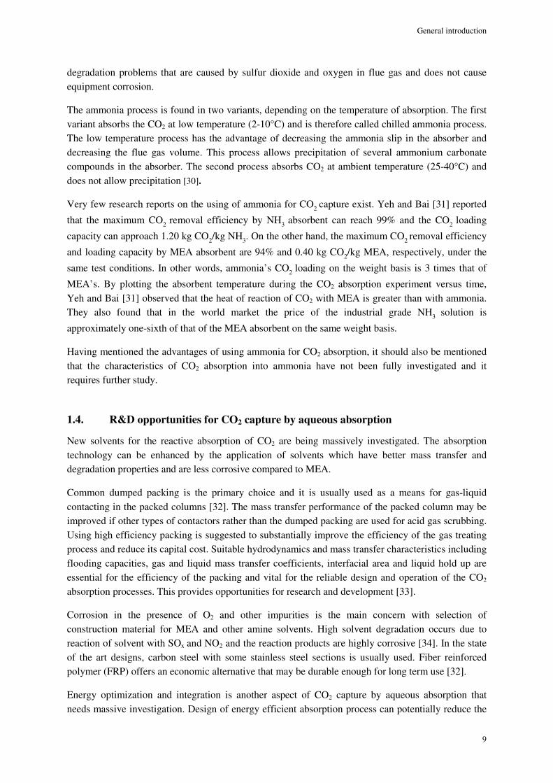
As shown in Figure 1.4, MEA solution contacts the flue gas from a conventional power plant. Through the scrubbing process CO2 is absorbed into the solvent and removed from the gas stream. Afterwards the CO2 rich solvent is pre-heated before being pumped into a regeneration column where it is heated and stripped off the CO2. The regenerated solvent is recycled to the absorber and the high purity CO2 stream off the top of the stripper column is then sent to a compressor where it is dried and compressed for transportation and storage.
Fig. 1.4. General scheme for CO2 capture by chemical absorption process using alkanolamines.
Even though, alkanolamines are the conventional solvents selected for CO2 scrubbing, they have several disadvantages when treating flue gas.
The major problems concerning the use of alkanolamines as absorbents for PCC are the amount of energy needed to regenerate the CO2-rich solvent and the size of the capture plant.
In case of the most used amine, MEA, beside the high energy consumption, there are other problems such as corrosion, solvent loss due vaporization and solvent degradation. The minor quantity of the amines emitted to air is not stable in the atmosphere and through degradation it forms hazardous
Chapter 1
8
substances that are toxic and represent risk of cancer. Among the degradation products are aldehydes, amides, nitrosamines and nitramines [23].
At present, using amine blends for CO2 capture is widely studied for application in new technologies. Among the examples are MEA-methyldiethanolamine (MDEA), MEA-piperazine (PZ) [24], MDEA-PZ [25] and blends of MDEA and triethylene tetramine. Several companies keep the amine mixture they use in their noble processes as secret recipes.
There are claims of significant capital and operating cost savings by the application of amine blends [23]. Chakravarti et al. [26] assert that among all the different operating cost constituents of the CO2 absorption process using MEA-based solvents, steam cost is the prevailing one. The reason for high energy consumption of MEA-based systems is the high heat of reaction of MEA with CO2. Using amine blends with concentrations as high as 50wt% is therefore recommended [26] implying that less water will need to be heated and consequently less steam is required for the process. Corrosion with MEA-based systems is significant at concentrations above 30 wt% due to degradation which does not allow for high MEA strength to be used in the process. Further, use of another amine such as MDEA together with MEA potentially allows for greater capacity and alleviates MEA degradation problems.
MEA can be loaded up to only 0.5 mol of CO2/mol of MEA as a result of the stable carbamate formed. Tertiary alkanolamines such as MDEA, can reach loadings of 1 mole of CO2/mole alkanolamine and the energy consumption for regeneration is lower, although the low rates of CO2 absorption make them infeasible for flue gas cleaning. Sartori and Savage [27] presented a group of amines, called sterically hindered amines, that have low carbamate stability, making loadings up to 1 feasible and the reaction rates are much higher compared to that of MDEA. Sterically hindered amines can be an attractive option for PCC.
Mitsubishi Heavy Industries have developed a new solvent, the proprietary KS-1, based on a sterically hindered amine to which an accelerator is added to improve its reaction kinetics. Beside the higher capacity compared to MEA, they claim that it has a 20% lower regeneration energy compared to the conventional MEA process [28].
Slow kinetics is the major problem with the strically hindered amines. Therefore, if no activator is used, the size of the absorber column is considerably larger compared to a faster amine like MEA. This would influence the overall cost of the CO2 removal system.
Abu-Zahra et al. [29] have done a preliminary study to estimate the CO2-capture costs and requirements by using 2-amino-2-methyl-1-propanol (AMP) solution as the capture solvent. Their overall evaluation shows the combined effect of significantly lower energy requirement and the larger size of the absorber column. The kinetics of AMP could be improved by using an accelerator like piperazine, which will result in a major reduction on the size of the absorber column. Adding an activator will certainly reduce the energy performance of AMP but this is anticipated to be trivial.
Aqueous ammonia
Processes using aqueous ammonia as solvent are promising alternatives for chemical absorption of CO2 from flue gases. Unlike the MEA process, the aqueous ammonia process does not have absorbent
General introduction
9
degradation problems that are caused by sulfur dioxide and oxygen in flue gas and does not cause equipment corrosion.
The ammonia process is found in two variants, depending on the temperature of absorption. The first variant absorbs the CO2 at low temperature (2-10°C) and is therefore called chilled ammonia process. The low temperature process has the advantage of decreasing the ammonia slip in the absorber and decreasing the flue gas volume. This process allows precipitation of several ammonium carbonate compounds in the absorber. The second process absorbs CO2 at ambient temperature (25-40°C) and does not allow precipitation [30].
Very few research reports on the using of ammonia for CO2 capture exist. Yeh and Bai [31] reported
that the maximum CO2 removal efficiency by NH3 absorbent can reach 99% and the CO2 loading
capacity can approach 1.20 kg CO2/kg NH3. On the other hand, the maximum CO2 removal efficiency
and loading capacity by MEA absorbent are 94% and 0.40 kg CO2/kg MEA, respectively, under the
same test conditions. In other words, ammonia’s CO2 loading on the weight basis is 3 times that of
MEA’s. By plotting the absorbent temperature during the CO2 absorption experiment versus time, Yeh and Bai [31] observed that the heat of reaction of CO2 with MEA is greater than with ammonia. They also found that in the world market the price of the industrial grade NH3 solution is
approximately one-sixth of that of the MEA absorbent on the same weight basis.
Having mentioned the advantages of using ammonia for CO2 absorption, it should also be mentioned that the characteristics of CO2 absorption into ammonia have not been fully investigated and it requires further study.
1.4. R&D opportunities for CO2 capture by aqueous absorption
New solvents for the reactive absorption of CO2 are being massively investigated. The absorption technology can be enhanced by the application of solvents which have better mass transfer and degradation properties and are less corrosive compared to MEA.
Common dumped packing is the primary choice and it is usually used as a means for gas-liquid contacting in the packed columns [32]. The mass transfer performance of the packed column may be improved if other types of contactors rather than the dumped packing are used for acid gas scrubbing. Using high efficiency packing is suggested to substantially improve the efficiency of the gas treating process and reduce its capital cost. Suitable hydrodynamics and mass transfer characteristics including flooding capacities, gas and liquid mass transfer coefficients, interfacial area and liquid hold up are essential for the efficiency of the packing and vital for the reliable design and operation of the CO2 absorption processes. This provides opportunities for research and development [33].
Corrosion in the presence of O2 and other impurities is the main concern with selection of construction material for MEA and other amine solvents. High solvent degradation occurs due to reaction of solvent with SOx and NO2 and the reaction products are highly corrosive [34]. In the state of the art designs, carbon steel with some stainless steel sections is usually used. Fiber reinforced polymer (FRP) offers an economic alternative that may be durable enough for long term use [32].
Energy optimization and integration is another aspect of CO2 capture by aqueous absorption that needs massive investigation. Design of energy efficient absorption process can potentially reduce the
Chapter 1
10
cost of the PCC process to a great extent [35]. Fluor has recently claimed development in PCC process based on MEA. The regeneration energy requirement for the improved process is reported to be 2.9 GJ/ton CO2 [36]. Compared to the estimated figure of 4.2 GJ/ton CO2 reported by Chapel et al. [37] this is a significant improvement which is claimed to be due to process integration and solvent improvement.
Among other aspects of the reactive PCC process that require investigation, process variable optimization, flow-sheet optimization and system simplification can also be notified.
1.5. Thesis motivation and outline
The main objective of this work was to develop a CO2 capture process design model and validating it against the literature experimental data.
The information provided in this thesis will help with defining the directions for future research activities for the improvement of the alkanolamine-based PCC processes and thus making it more attractive to be applied for the greenhouse gas emission control.
The work presented in this thesis is done in two main phases:
Phase 1: Thermodynamic Modeling An accurate rate model is required to simulate the reversible absorption process. The rate model should be coupled with a precise thermodynamic model in order to calculate the driving forces for mass transfer.
The purpose of the first phase of the work was to apply the in-house model, extended UNIQUAC, to estimate various thermodynamic properties of the alkanolamine systems required for the design of the CO2 capture plants. In addition, the model proved capable to represent different types of thermodynamic properties of the aqueous CO2-alkanolamin systems in a broad range of conditions using only one unique set of parameters. It has been shown that extended UNIQUAC can accurately represent physical and chemical equilibria (excess enthalpy, Vapor-liquid equilibria, solid-liquid equilibria and speciation) over a wide range of conditions.
Phase 2: Modeling the Absorber
Despite the fact that the acid gas absorption process has been studied for many years and there have been many modeling approaches adopted by researchers, the available models need to be enhanced and there is room for developing new reliable ones.
In this project, the rate-based steady state model proposed by Gabrielsen et al. [38] for the design of the CO2- 2-amino-2-methyl-propanol (AMP) absorbers is adopted and improved for the design of the CO2- monoethanolamine (MEA) absorber.
The model has been successfully applied to CO2 absorber packed columns and validated against pilot plant data with good agreement.
General introduction
11
References
[1] Intergovernmental Panel on Climate Change (IPCC), Summary for Policymakers. In: Climate Change 2007: The Physical Science Basis, Cambridge University Press, 2007. [2] International Energy Agency (IEA), World Energy Outlook 2007, China and India Insight, IEA Publications, 2007. [3] S. M. Forbes, P. Verma, T. E. Curry, M. J. Bradley, S. J. Friedmann, S. M. Wade, CCS Guidelines, Guidelines for Carbon Dioxide Capture, Transport, and Storage, World Recourses Institute, 2008. [4] R. C. Sekar, Carbon Dioxide Capture from Coal-Fired Power Plants: A Real Options Analysis, Massachusetts Institute of Technology, MIT LFEE 2005-002 RP, 2005. [5] Intergovernmental Panel on Climate Change (IPCC), Climate Change 2007: Synthesis Report, IPCC, Geneva, Switzerland. pp 104, 2007. [6] Retrofitting of Coal-Fired Power Plants for CO2 Emissions Reductions, An MIT Energy Initiative Symposium, Massachusetts Institute of Technology, 2009. [7] Energy Information Administration (EIA), Emissions of Greenhouse Gases Report, US Department of Energy Report, DOE/EIA-0573, 2006, 2007. [8] International Energy Agency (IEA), Contribution of Renewables to Energy Security, IEA Information Paper, France, 2007. [9] D. R. Cole, E. H. Oelkers, Elements 4 (2008) 311-317. [10] The Future of Coal: Options for a Carbon Constrained World, MIT 2007, Massachusetts Institute of Technology, Cambridge MA., 2007. [11] K. Jordal, M. Anheden, J. Yan, L. Strömberg, Oxyfuel Combustion for Coal-Fired Power Generation with CO2 Capture- Opportunities and Challenges, 7th International Conference on Greenhouse Gas Technologies, Vancouver, Canada, 2004. [12] L. Christopher, Capturing CO2, International Energy Agency (IEA), Greenhouse Gas R&D Programme 2007, Separations Research Program, 2007. [13] Intergovernmental Panel on Climate Change (IPCC), IPCC Special Report on Carbon Dioxide Capture and Storage, Cambridge University Press, UK. pp 431, 2005. [14] S. Sridhar, B. Smitha, T. M. Aminabhavi, Sep. Purif. Technol. 36 (2) (2007) 113-174. [15] S. Choi, J. H. Drese, C. W. Jones, ChemSusChem 2 (2009) 796-854. [16] M. Kanniche, C. Bouallou, Appl. Therm. Eng. 27 (2007) 2693-2702. [17] D. deMontigny, Post-Comustion Capture, Presentation for IEA Greenhouse Gas Summer School, Canada, 2008. [18] M. Pellerano, P. Pré, M. Kacem, A. Delebarre, Energy Procedia 1 (2009) 647-653. [19] M. Fang, Post-combustion for CO2 Capture, Presentation at COACH Autumn School on CCS in China, 2009. [20] A. B. Rao, E. S. Rubin, Environ. Sci. Technol. 36 (2002) 4467-4475. [21] H. Herzog, An Introduction to CO2 Separation and Capture Technologies, MIT Energy Laboratory Working Paper, Massachusetts Institute of Technology, 1999. [22] M. Abu Zahra, PhD Thesis, Technische Universiteit Delft, 2009. [23] R. Shao, A. Stangeland, Amines Used in CO2 Capture - Health and Environmental Impacts, Bellona Report, The Bellona Foundation, Norway, 2009. [24] M. Nainar, A. Veawab, Energy Procedia 1 (2009) 231-235. [25] S. Bishnoi, G. T. Rochelle, Ind. Chem. Eng. Res. 41 (2002) 604-612. [26] S. Chakravarti, A. Gupta, B. Hunek, Advanced Technology for the Capture of Carbon Dioxide from Flue Gases, First National Conference on Carbon Sequestration, Washington, DC, 2001. [27] G. Sartori, D. W. Savage, Ind. Eng. Chem. Fundam. 22 (1983) 239-249. [28] N. Imai, Advanced Solvent to Capture CO2 From Flue Gas, 2nd International Forum on Geological Sequestration of CO2 in Deep, Unmineable Coal Seams, 2003. [29] M. R. M. Abu-Zahra, P. H. M. Feron, P. J. Jansens, E. L. V. Goetheer, Int. J. Hydrogen Energy 34 (2009) 3992-4004. [30] V. Darde, K. Thomsen, W. J. M. van Well, Stenby E. H., Energy Procedia, 1 (2009) 1035-1042. [31] A. C. Yeh, H. Bai, The Science of Total Environment, 228 (1999) 121-133. [32] G. T. Rochelle, S. Bishnoi, S. Chi, H. Dang, J., CO2 Capture from Flue Gas by Aqueous Absorption/Stripping, Final Report for P.O. No. DE-AF26-99FT01029, U.S. Department of Energy, 2001. [33] S-Y Park, B-M Min, J-S Lee, S-C Nam, K-H Han, J-S Hyun, Prepr. Pap.-Am. Chem. Soc., Div. Fuel Chem. 49 (1) (2004) 249-250. [34] J. Davidson, K. Thambimuthu, Proceedings of GHGT, 7 (2004) 5-9. [35] A. Aboudheir, Industrial Design and Optimization of CO2 Capture, Dehydration and Compression Facilities, HTC Purenergy Gavin McIntyre, Bryan Research & Engineering, Gas Processors Association (GPA) , 2009. [36] S. Reddy, Econamine FG PlusSM Technology for Post-Combustion CO2 Capture, Presentation for the 11th Meeting of the International Post-Combustion CO2 Capture Network, Vienna, Austria, 2008. [37] D. Chapel, J. Ernst, C. Mariz, Can. Society of Chem. Eng. Oct 4-6 (1999). [38] J. Gabrielsen, M. L. Michelsen, G. M. Kontogeorgis, E. H. Stenby, AICHE J. 52 (10) (2006) 3443-3451.
22
THERMODYNAMIC MODELING OF AQUEOUS CO2+ALKANOLAMINE SOLUTIONS
The extended UNIQUAC model [Thomsen, Rasmussen, Chem. Eng. Sci. 54 (1999) 1787-
1802] was applied to the thermodynamic representation of carbon dioxide absorption in aqueous
monoethanolamine (MEA), methyldiethanolamine (MDEA) and varied strength mixtures of the two
alkanolamines (MEA-MDEA). For these systems, altogether 13 interaction model parameters are
adjusted. Out of these parameters, 11 are temperature dependent.
All the essential parameters of the model are simultaneously regressed to a collective set of data on
the single MEA and MDEA systems.
Different types of data are used for modeling and they cover a very wide range of
conditions. Vapor-liquid equilibrium (VLE) data for the aqueous alkanolamine systems containing
CO2 in the pressure range of 3-13000 kPa and temperatures of 25-200ºC are used. The model is also
regressed with the VLE and freezing point depression data of the binary aqueous alkanolamine
systems (MEA-water and MDEA-water). The two just mentioned types of data cover the full
concentration range of alkanolamines from extremely dilute to almost pure. The experimental freezing
point depression data down to the temperature of -20ºC are used. Experimental excess enthalpy (HE)
data of the binary MEA-water and MDEA-water systems at 25, 40, 65 and 69ºC are used as well. In
order to enhance the calculation of the infinite dilution activity coefficients of MEA and MDEA, the
pure alkanolamines vapor pressure data in a relevant temperature range (up to almost 230ºC) are
included in the parameter estimation process.
The previously unavailable standard state properties of the alkanolamine ions appearing in
this work i.e. MEA protonate, MEA carbamate and MDEA protonate are determined.
The concentration of the species in both MEA and MDEA solutions containing CO2 are
predicted by the model and in the case of MEA compared to NMR spectroscopic data.
Using only one set of parameters for correlation of different thermodynamic properties, the
model has represented the experimental data with good precision [Faramarzi, Kontogeorgis,
Thomsen, Stenby, Fluid Phase Equilib. 282 (2) (2009) 121-132].
Thermodynamic modeling of aqueous CO2+alkanolamine solutions
13
2.1. Introduction
The well established process of chemical absorption into aqueous alkanolamines is considered a prospective option for post-combustion capture of CO2 from fossil-fueled power plants.
To properly simulate the reversible absorption process, a rate model is needed. However, it is essential to incorporate an accurate thermodynamic model with a rate model to calculate the driving forces for mass transfer correctly.
The problem with thermodynamic modeling of acid gas treating plants is that the vapor-liquid equilibrium (VLE) data reported for these systems are not generally very consistent.
Although a large body of experimental data for CO2-alkanolamine-H2O systems has been reported in the literature, a small portion of the VLE data are in the low acid gas pressure range where it is perhaps most important. Therefore, a thermodynamic property model capable of accurate representation of VLE is essential for a successful design and simulation. A successful VLE model cannot only be used in equilibrium stage design calculations, but also in the rate based models in which liquid phase concentration enter into kinetic expressions affecting mass transfer at vapor-liquid interface.
Study of solvent loss in acid gas absorption units by means of alkanolamine absorbents has been a concern from the economical point of view. Recently, the concerns about the environmental hazards of outflow of amines to outside of the absorption system, has given the problem of amine loss a new dimension. McLees [1] claims that the potential environmental hazards of amine release to the atmosphere has to be the main concern with amine volatility. The reason is, while being in the atmosphere amines can go through different reactions as the result of which many hazardous compounds are produced.
In 1994, Stewart and Lanning [2] reported an annual amount of 95 MMlb solvent loss in alkanolamine gas and liquid treating plants only in the U.S. The loss happening in amine plants can happen due to variety of reasons. Although, the major factor in the gas treating plants is amine volatility. For this reason study of the binary VLE behavior of amine-water systems can provide a good basis for selecting optimum process conditions to minimize amine loss. However, the indispensable data on the VLE of alkanolamine-H2O systems are limited in the open literature. Moreover, other data on the binary alkanolamine-H2O systems such as the excess enthalpy are scarce and those available from a handful of sources show discrepancies.
Developing empirical correlations based on the existing data, using excess Gibbs energy based activity coefficient models and application of equations of state which are based on excess Helmholtz energy are three different approaches for thermodynamic modeling of chemical absorption of CO2.
Correlations could be very precise and calculations are often not cumbersome. Yet, empirical expressions typically fail when being extrapolated to conditions other than what they are based on.
One example is the simple correlation of Kent and Eisenberg [3] for CO2 solubility in aqueous MEA and diethanolamine (DEA). Gabrielsen et al. [4] presented another very simple correlation for the calculation of the partial pressure and enthalpy of absorpt ion of CO2 in MEA, DEA and MDEA.
CChhaapptteerr 22
14
An equation of state can be easily extended to predict the solubility of more than a single gas in the solution; it also can be used to calculate the properties such as density of both liquid and vapor phases. However, the performance of an equation of state to a great extent depends on the mixing rules chosen and an unsuitable choice can lead to erroneous results. Chunxi and Fürst [5], Solbraa [6] and Huttenhuis et al. [7] have used the Fürst and Renon [8] equation of state to represent CO2 solubility in aqueous MDEA. Solbraa [6] has also applied the Cubic Plus Association (CPA) model proposed by Kontogeorgis et al. [9] for the MDEA system.
Using the electrolyte activity coefficient models is the most common alternative. Posey and Rochelle [10] applied electrolyte NRTL (e-NRTL) model to predict the CO2 solubility in MDEA solution. This model had been used earlier by Austgen et al. [11, 12] for MEA, DEA and mixtures of MDEA with MEA and DEA.
The purpose of the present work is to apply the extended UNIQUAC model [13] to estimate various thermodynamic properties of the alkanolamine systems required for the design of CO2 capture plants. In addition, the capability of the model to represent different types of thermodynamic properties in a broad range of conditions using only one unique set of parameters is investigated.
Moreover, the standard state Gibbs free energy of formation and enthalpy of formation for the ions that MEA and MDEA form in aqueous CO2 solutions are calculated. These formerly unavailable properties are required for thermodynamic calculations of MEA and MDEA systems.
The model parameters are determined based on a large number of data covering the temperature and pressure of the reversible absorption process (both absorption and desorption) and exceeding far beyond. Therefore, these parameters can be used even if the model is applied to other processes such as natural gas purification.
Compared to the previous modeling attempts by other authors, a larger number of properties and a considerably extensive range of conditions are addressed in this work.
2.2. Chemical and phase equilibria
2.2.1. Speciation equilibria
CO2 reacts with alkanolamines in aqueous solutions. The chemical equilibrium reactions considered in this work are:
Aqueous CO2 system:
2 ( )H O l H OH+ −↔ + (2.1)
2 2 3( ) ( )CO aq H O l H HCO+ −+ ↔ + (2.2)
23 3HCO H CO− + −↔ + (2.3)
MEA system:
2 3 2( ) ( )RNHCOO H O l HCO RNH aq− −+ ↔ + (2.4)
Thermodynamic modeling of aqueous CO2+alkanolamine solutions
15
3 2 ( )RNH H RNH aq+ +↔ + (2.5)
(R: -CH2CH2OH)
MDEA system:
´ ´2 2 ( )R R NH H R R N aq+ +↔ + (2.6)
(R´: -CH3)
The symmetrical convention for water and mole fraction (rational) based asymmetrical convention for all other species is adopted. Based on the symmetrical convention, the activity coefficient of water which is considered to be the only solvent by the model is unity in the pure component state at all temperatures.
The chemical potential of water in the liquid phase is expressed as
( )0 0ln lnw w w w w w
RT a RT xµ µ µ γ= + = + (2.7)
where 0w
µ is the standard state chemical potential for pure liquid water at system temperature and
pressure, wa is the activity, R(Jmol-1K-1) the gas constant, T(K) is the temperature and w
γ is the
symmetrical activity coefficient of water.
The asymmetrical convention is based on the constraint that the activity coefficient of a solute compound is unity at infinite dilution. The chemical potential for the solute i (all the compounds other than water including alkanolamines) is written as
( )*, *,lnx x
i i i iRT xµ µ γ= + (2.8)
where *,xi
µ is the asymmetrical standard state chemical potential for the solute i and *,xi
γ is the
asymmetrical rational activity coefficient of i. This is a hypothetical ideal state for the pure solute i.
The speciation equilibria can be expressed as
0
, lnj
i j i
i
Ga
RTν
∆− =∑ (2.9)
∆Gj0
(J mol-1
) is the variation in the standard state chemical potential caused by the equilibrium
reaction j at the certain temperature T (K). ai is the activity of component i and ,i jν is the
stochiometric coefficient of component i involved in reaction j.
CChhaapptteerr 22
16
2.2.2. Vapor-liquid equilibria
For the volatile compounds, the vapor-liquid equilibria can be written as
( ) ( )2 2CO g CO aq↔ (2.10)
( ) ( )MEA g MEA aq↔ (2.11)
( ) ( )MDEA g MDEA aq↔ (2.12)
( ) ( )2 2H O g H O l↔ (2.13)
For the compounds in the vapor phase, the chemical potential is given by:
0
0
lnv g
i i i i
PRT y
Pµ µ ϕ
= +
(2.14)
where 0g
iµ is the standard state chemical potential of the component i in the vapor phase defined as
the pure ideal gas at one bar and the temperature T. P0 is the standard state pressure of one bar. iy
and iϕ are the vapor phase mole fraction and the fugacity coefficient of i and P is the total pressure.
The condition of equilibrium between the aqueous and gas phases is:
aq v
i iµ µ= (2.15)
where aq
iµ and v
iµ are the chemical potentials of i in the aqueous and the gas phase, respectively.
On the basis of the phase equilibrium condition and also the expressions for the chemical potential (2.7), (2.8) and (2.14) the following expression can be written:
0
0
ln i i
i i
y PG
RT x P
ϕ
γ
∆− = (2.16)
where
0 0 0g aq
i iG µ µ∆ = − (2.17)
is the chemical potential change due to the transfer of one mole of component i from liquid to the
vapor phase. 0i
µ and iγ are based on the symmetrical approach for water and asymmetrical approach
for the solute species.
The equilibrium equation for speciating compounds should be written in the form of equation (2.9) and equations (2.10)-(2.13) should be expressed in the form of equation (2.16). In order to calculate
Thermodynamic modeling of aqueous CO2+alkanolamine solutions
17
the equilibrium composition of the system, equations (2.1)-(2.6) and (2.10)-(2.13) have to be solved simultaneously.
The bubble point pressure of an electrolyte solution can be found by simultaneously solving equations in the form of equation (2.16) for all the volatile species.
2.2.3. Pure component vapor pressure
In this work, the extended UNIQUAC model is also used for the correlation of the pure alkanolamine vapor pressure. Following equation (2.16) for the condition of vapor-liquid equilibria for a pure alkanolamine,
0alkanolamine alkanolamine
*,alkanolamine alkanolamine 0
lnx
y PG
RT x P
ϕ
γ
∆− = (2.18)
where the asymmetrical activity coefficient of alkanolamine can be calculated as
*, alkanolaminealkanolamine
alkanolamine
x γγ
γ ∞= (2.19)
According to the symmetrical convention the activity coefficient for the pure alkanolamine is
( )alkanolamine alkanolamine1 1xγ = → (2.20)
alkanolamineγ ∞ is the infinite dilution activity coefficient calculated by the model. Considering that the
mole fraction of alkanolamine in both phases is unity equation (2.18) can therefore be written as
0alkanolamine alkanolamine
0
lnPG
RT P
ϕ γ ∞∆− = (2.21)
using which the pure alkanolamine vapor pressure can be calculated.
2.2.4. Pure component vapor pressure
The experimental freezing point depression data available are within the temperature range where the only solid phase formed is ice. Therefore, the condition of solid-liquid equilibria reduces to
0
ln w
i
Ga
RT
∆− =∑ (2.22)
where aw is the activity coefficient of water and ∆G0 (J mol-1) is the change in chemical potential of
liquid water by shifting to ice.
CChhaapptteerr 22
18
2.3. Standard state properties
In order to evaluate the chemical potentials of water and solutes according the standard state chemical potentials need to be known. The required standard state properties: Gibbs free energy of formation, enthalpy of formation and heat capacities for most of the species present in the aqueous solutions studied in this work are obtained from NIST tables [14]. The standard state chemical potentials from NIST tables are mainly reported for 25ºC. At temperatures other than 25ºC, they are calculated using the Gibbs-Helmholtz equation and enthalpy and heat capacity data. These standard-state properties are reported with reference to the molality standard state and, therefore need to be converted to the unsymmetric mole fraction scale. This conversion is achieved with the relation:
* lnm
i i wRT Mµ µ= + (2.23)
m
iµ is the molality based standard state for the component i. The standard-state chemical potentials at
temperatures different from 298.15 K are evaluated using the Gibbs–Helmholtz equation:
*
2
i
f iHRTd
dT RT
µ ∆ = − (2.24)
Chen and Song [35] describe he standard-state heat capacity of ionic solute i, *,p i
C , by the three-
parameter correlation:
( )*
, 200i
p i i i
cC a bT
T= + +
− (2.25)
where ai, bi and ci are adjustable parameters. This standard-state heat capacity is used for evaluating
the temperature dependence of the standard-state enthalpy of formation f iH∆ in equation (2.24), and
for calculating the heat capacity of electrolyte solutions.
Kim et al. [15] reported the Gibbs energy and enthalpy of dissociation of MEA protonate according to equation (2.5). Their data were used to calculate the initial values for the standard state properties of the MEAH+ ion.
Based on their experimental measurements, Aroua et al. [16] presented a correlation for the temperature dependence of the thermodynamic equilibrium constant of the MEA carbamate formation reaction which is the reverse of reaction (4). Their correlation was used to estimate the values of the Gibbs energy and enthalpy of formation of the MEA carbamate ion at the temperature of 25ºC. The estimated properties were used as the initial guess for starting the calculations.
The Gibbs energy and enthalpy of dissociation of protonated MDEA according to equation (2.6) were determined using the chemical equilibrium data published by Perez-Salado Kamps and Maurer [17].
Finally, the noted standard state properties for MEA(aq), MEAH+, MEA carbamate, MDEA(aq) and MDEAH+ were adjusted to all types of experimental data available in the database.
Thermodynamic modeling of aqueous CO2+alkanolamine solutions
19
For the ions MEAH+, MEA carbamate, and MDEAH+ the heat capacities were not available in the standard tables or in the open literature. For these ions the heat capacities were assumed to be zero because adjusting them to experimental data did not improve the modeling results.
The standard state properties of MEA (g) and MDEA (g) are taken from the DIPPR database [18].
2.4. Model
The majority of the thermodynamic models for electrolyte solutions have two main constituting terms. They are usually comprised of a term for short-range interactions and a term for long-range, electrostatic interactions. In order to correctly model electrolyte systems, all different types of interactions should be taken into account. The possible interactions are ion-ion, ion-dipole, dipole-dipole and molecule-molecule. The potential energy caused by ion-ion interactions is proportional to the inverse of the separation distance r. Electrostatic ionic interactions therefore are effective over comparatively a long distance and thus called long range interactions. The potential energy caused by molecule-molecule interactions is proportional to the sixth power of the inverse separation distance, 1/r6, and consequently called short-range interactions. There are also the interactions which are often called the intermediate interactions, ion-dipole and dipole-dipole interactions are in this category and are proportional to 1/r2 and 1/r3 respectively.
Most models are structured with terms representing only long range or intermediate/short range interactions [19].
The Debye and Hückel theory [20] is often the basis for the description of the electrostatic interactions where they are considered within an ideal solution of charged particles. This hypothesis was the foundation of the first successful model for the electrostatic interactions between the ions in aqueous electrolyte systems. However, with the Debye-Hückel model, the short range interactions are not taken into account. In this model, the solvent only has a function due to its relative permittivity and its density. Therefore, the interactions between water which is the most important constituent of an aqueous system, and other components are not explained by this theory.
To apply the Debye–Hückel theory to nonideal systems, it has to be combined with a term for short-range interactions. The Pitzer model [21] combines a Debye–Hückel term with a virial expansion of terms in molality [22]. The electrolyte nonrandom two-liquid (NRTL) model [23] combines the Pitzer-Debye- Hückel term with the NRTL local composition model [24]. In the systems where ions are present, the local composition theory is customized to be used for ions. The parameters of the electrolyte NRTL model are salt-specific. The extended universal quasichemical (UNIQUAC) model [25] combines a Debye–Hückel term with the UNIQUAC local composition model. The local composition term is identical for ions and other components, and the model parameters are ion-specific. An alternative term for long-range electrostatic interactions has been derived from the mean spherical approximation (MSA) theory. This term has mainly been applied in combination with short-range interactions derived from cubic equations of state [26].
The extended UNIQUAC model as presented by Thomsen and Rasmussen [13] is used for the thermodynamic calculations of this work. This model was the first time proposed by Sander et al. [27]. It is a local composition model which in its original form is the combination of a modified UNIQUAC equation that takes into account the concentration dependency of UNIQUAC interaction
CChhaapptteerr 22
20
parameters and a Debye-Hückel type term. Originally, the model had been developed for calculation of the influence of salt on the vapor-liquid equilibria of the mixed solvent systems. Later Nicolaisen et al. [28] presented a simplified form of the extended UNIQUAC model which is the combination of the original UNIQUAC equation as proposed by Abrams and Prausnitz [29] and Maurer and Prausnitz [30] and the Debye-Hückel term as suggested by Fowler and Guggenheim [31]. A significant advantage of the Extended UNIQUAC model compared to models like the Pitzer model is that temperature dependence is built into the extended UNIQUAC model. This enables the model to also describe thermodynamic properties that are temperature derivatives of the excess Gibbs function, such as heat of mixing and heat capacity [19]. Compared to the electrolyte NRTL model the expressions for the activity coefficients in the extended UNIQUAC model are significantly simpler and require less time for programming. The use of a Pitzer-Debye-Hückel term instead of the Extended Debye-Hückel term does not make much difference. The NRTL local composition model only has an enthalpic term and has no volume and surface area fractions. The use of salt specific parameters rather than ion specific parameters requires that a suitable mixing rule is applied. Otherwise calculations of solution properties would depend on how the composition of the solution is defined.
When an electrolyte solution with a mixed solvent system is considered, modeling the system becomes more difficult than the case of a system with single solvent. The problem which arises is that in such systems, the standard chemical potential of ions which are required to calculate phase euilibria, are dependent on the composition of the solute free solvent.
Pérez-Salado Kamps [32] has developed a very elaborate model for the mixed solvent electrolyte systems considering the dependency of standard chemical potential of ions on the composition of the solvent. This model comprises of the original UNIQUAC model for considering the interactions between the solvent molecules and an extended form of the equation of Pitzer [21] for the excess Gibbs energy to consider the interactions between the neutral or ionic solutes added to the system. The extended form of the Pitzer’s excess Gibbs energy allows for any single or mixed solvent system. If the parameters of the extended Gibbs energy equation are considered temperature, pressure and solvent composition dependent, the model becomes computationally expensive as many adjustable parameters are introduced to the model. Moreover, Pérez-Salado Kamps [32] considered the dependence of the dielectric constant (relative permittivity) on the composition of solvent mixture through application of a Redlich-Kister type of expansion which increases the number of parameters of the model. Considering the solvent as a mixture makes the thermodynamic calculations of the system very complicated. Moreover, as the only results presented [32] are for the methanol and water system, it is unclear how the model works for other mixed solvents.
When the extended UNIQUAC model as it is presented by Thomsen [33] is applied to the electrolyte solutions constituted by a mixture of solvents, one solvent (water) is treated as solvent with symmetrical convention and other solvents are accounted for as solutes for which asymmetrical convention is adopted [34]. Using this approach would enable the user to define appropriate standard states chemical potentials for solutes without having to consider their dependency on solute free solvent composition. This way the calculation of phase equilibria becomes very simpler. Also by applying the assumption noted, in the Extended UNIQUAC model the relative permittivity can be considered independent of the solvent mixture composition yet with acceptable accuracy. Therefore, compared to the model of Pérez-Salado Kamps [32] there are fewer adjustable parameters in the extended UNIQUAC model. By only using the pure water properties in the Debye-Hückel equation, i.e density and dielectric constant of water instead of the solvent mixture, the extended UNIQUAC
Thermodynamic modeling of aqueous CO2+alkanolamine solutions
21
model does not result in large deviations for solutions. Although, it should be mentioned that solutions may have quite different Debye-Hückel parameters compared to that of water but the overall results are comparable in accuracy. The electrolyte NRTL model as proposed by Chen et al. [23] has also been used for description of excess Gibbs energy of electrolyte solutions for single and mixed solvent systems. Chen and Song [35] define a segment interaction concept to provide a framework to consider the attractive interaction of ions with the hydrophilic segment of organic solvents and the repulsion of ions with the hydrophobic segments of organic solvents (though this definition sounds unnecessary and does not change the basis of electrolyte NRTL). Thomsen [19] claims that the use of Pitzer-Deby-Hückel instead of Deby-Hückel term only adds to the complexity of the electrolyte NRTL model while not significantly improving its performance. The reference state for the chemical potential of solutes for the mixed solvents in electrolyte NRTL is infinite dilution in water [34] which makes the model simpler than that of Pérez-Salado Kamps [32] but comparing to extended UNIQUAC the expressions for the activity coefficients are more complex which makes the electrolyte NRTL model difficult to program.
Extended UNIQUAC has been successfully used for many different solvent mixtures such as solution of carbon dioxide in methyl-di-ethanolamine and water [36] and for CO2 in ammonia and water [13] which makes it interesting to apply for carbon capture process.
2.4.1. Extended UNIQUAC
The extended UNIQUAC model expresses the excess Gibbs energy as the combination of three terms contributing to the total excess Gibbs energy: the entropic and enthalpic terms of the original UNIQUAC equation to consider the non-electrostatic interactions and, the electrostatic term (Debye Hückel):
UNIQUAC entropic UNIQUAC enthalpic Debye-Hückel
E E E EG G G G
RT RT RT RT
= + +
(2.26)
The first term i.e. the entropic term, is to describe the deviation from ideality due to the shapes and sizes of individual species in the solution and it is determined by the composition. This term is given as
UNIQUAC entropic
ln ln2
E
i i
i i i
i ii i
G zx q x
RT x
φ φ
θ
= −
∑ ∑ (2.27)
where z is the coordination number arbitrarily set to 10. Volume fraction iφ and area fraction i
θ are
i i i ii i
j j j j
j j
x r x q
x r x qφ θ= =
∑ ∑ (2.28)
xi is the mole fraction of component i. The volume parameter ri and the surface area parameter qi are treated as adjustable parameters in this work.
CChhaapptteerr 22
22
The residual or the enthalpic term, is the other short range term of the UNIQUAC equation which is meant to take into account the energetic interactions between like and unlike species,
UNIQUAC enthalpic
lnE
i i j ji
i j
Gx q x
RTψ
= −
∑ ∑ (2.29)
where ji
ψ is
exp ji ii
ji
u u
Tψ
− = −
(2.30)
The adjustable interaction parameters (uij) of the UNIQUAC enthalpic term are assumed to be temperature dependent and are fitted to the following function of temperature
0 ( 298.15)T
ji ji jiu u u T= + − (2.31)
The Debye-Hückel expression used is the simplification of the original term given by Debye and Hückel [20] as suggested by Fowler and Guggenheim [31] for the electrostatic contribution to the excess Gibbs energy:
( )2
3Debye-Hückel
4ln 1
2
E
w w
G A b Ix M b I b I
RT b
= − + − +
(2.32)
xw and Mw are the mole fraction and molar mass of water respectively. The parameter b is considered to be a constant equal to 1.50 (kg/mol)1/2. A is the Debye-Hückel constant given by
( )
123
3
04 2A r
F dA
N RTπ ε ε
=
(2.33)
where F(Cmol-1) is the Faraday’s constant, NA(mol-1) is Avogadro’s number, ε0(C2J-1m-1) is the
vacuum permittivity, R(Jmol-1K-1) the gas constant and T(K) is the temperature. d(kgm-3) and εr are the density and the relative permittivity of the solution respectively.
The Debye-Hückel parameter is considered temperature dependent which for the temperature range of 273.15 to 383.15 K can be written as
1 13 5 2 2 21.131 1.335 10 ( 273.15) 1.164 10 ( 273.15)A T T kg mol
−− − = + × × − + × × − (2.34)
I(mol/kg H2O) is the ionic strength expressed as:
212 i i
i
I m z= ∑ (2.35)
Thermodynamic modeling of aqueous CO2+alkanolamine solutions
23
where mi(mol/kg H2O) and zi are the molality and the charge number of ionic species i respectively.
There are no adjustable parameters in the Debye-Hückel term and the Debye-Hückel parameter is based on the density and dielectric constant of pure water. This means that the effect of alkanolamine and other solute species on the dielectric constant of the solution is not considered and also by considering water as the single solvent, the density of pure water rather than that of the solution can be used. This strategy simplifies the calculations while the reasonable precision of the model is sustained.
The vapor phase fugacities are calculated using the Soave-Redlich-Kwong (SRK) equation of state. There are also no parameters adjusted for the SRK equation.
Now that all the terms contributing to the total excess Gibbs energy are defined, the activity coefficients of the molecular and ionic species are obtained by partial molar differentiation of the Gibbs energy expressions
, ,
ln
j ì
E
i
i
P T n
nG
RT
nγ
≠
∂ =
∂
(2.36)
The symmetrical activity coefficient for water and the asymmetrical activity coefficients for the ions can be calculated as
entropic enthalpic Debye-Hückel
* *,entropic *,enthalpic *,Debye-Hückel
ln ln ln ln
ln ln ln lnw w w w
i i i i
γ γ γ γ
γ γ γ γ
= + +
= + + (2.37)
2.5. Excess enthalpy
The Gibbs-Helmholtz equation is used for calculation of the symmetrical excess enthalpy of alkanolamine-water solutions. The equation defines the temperature dependence of the excess Gibbs energy and therefore also of the activity coefficients:
alkanolamine
alkanolamine2
, ,
,
ln ln
E
E
ww
P x P x
P x
G
T Hx x
T T T T
γ γ
∂
∂ ∂ = − = + ∂ ∂ ∂
(2.38)
The extended UNIQUAC model used in this work, determines the asymmetrical activity coefficient of alkanolamine which can be converted to the symmetrical activity coefficient using equation (2.19).
CChhaapptteerr 22
24
2.6. Estimation of parameters
A least square minimization was performed in order to estimate the model parameters. The aim was to minimize the following weighted sum of squared residuals:
( ) E
202 2calc exp E,calc E,exp
expVLE data SLE dataH data
ln
12 0.250.05 0.01
i i
i
G RT aP P H H
SRx RTP
ν ∆ + − − = + + +
∑∑ ∑ ∑
(2.39)
The experimental values and those calculated by the model are indicated by “exp” and “calc” respectively. P(bar) is the bubble point pressure, HE(Jmol-1) the excess enthalpy and ∆G
0 (J mol-1) is the change in the chemical potential by transferring one mole from liquid to solid phase and R(mol/kg H2O) is the gas constant
The factors 0.05, 12 and 0.25, for the three terms of the S function, are weighting factors which are chosen so that the difference between experimental and calculated data would lead to reasonable squared residuals for each data-type. 0.01 bar is added to the denominator of the VLE data term in order not to give too much weight to the very low pressure data. x=1K is included in the excess enthalpy term in order to make the equation dimensionless.
In this work, the volume and surface area parameters, r and q respectively, for MEA, MEAH+, MEA carbamate, MDEA and MDEAH+ are determined by fitting to experimental data.
The binary interaction parameters that are chosen to be adjusted are regressed to all types of experimental data in order to get a well-rounded model as well as to ensure accurate representation of different properties.
2.7. Parameter regression database
Some of the experimental data used for the parameter regression of this work were given in the volumetric concentration units. The data of Isaacs et al. [37], Lee et al. [38] and Maddox et al. [39] for the ternary VLE of CO2-MEA-water system, those of Chakma and Meisen [40], Jou et al. [41,42] and Si Ali and Aroua [43] for the VLE of CO2-MDEA-water system and Austgen et al. [12] and Maddox et al. [39] for both systems were expressed in volumetric units. Experimental densities of amine solutions or reliable density correlations were needed to convert them to weight percent. Table 2.1 summarizes the experimental density data sets surveyed in this work.
Referring to the noted experimental data, the densities of the amine solutions of the present work appeared to be very close to the density of water at the conditions of interest. Therefore, aqueous alkanolamine densities are assumed to be the same as that of water at each specific temperature.
Except for only few datasets, the experimental VLE data of the systems containing CO2 were expressed in the form of CO2 partial pressure. However, the calculated pressures that were compared to experimental pressures in the sum of the squared residuals are bubble point pressures. The
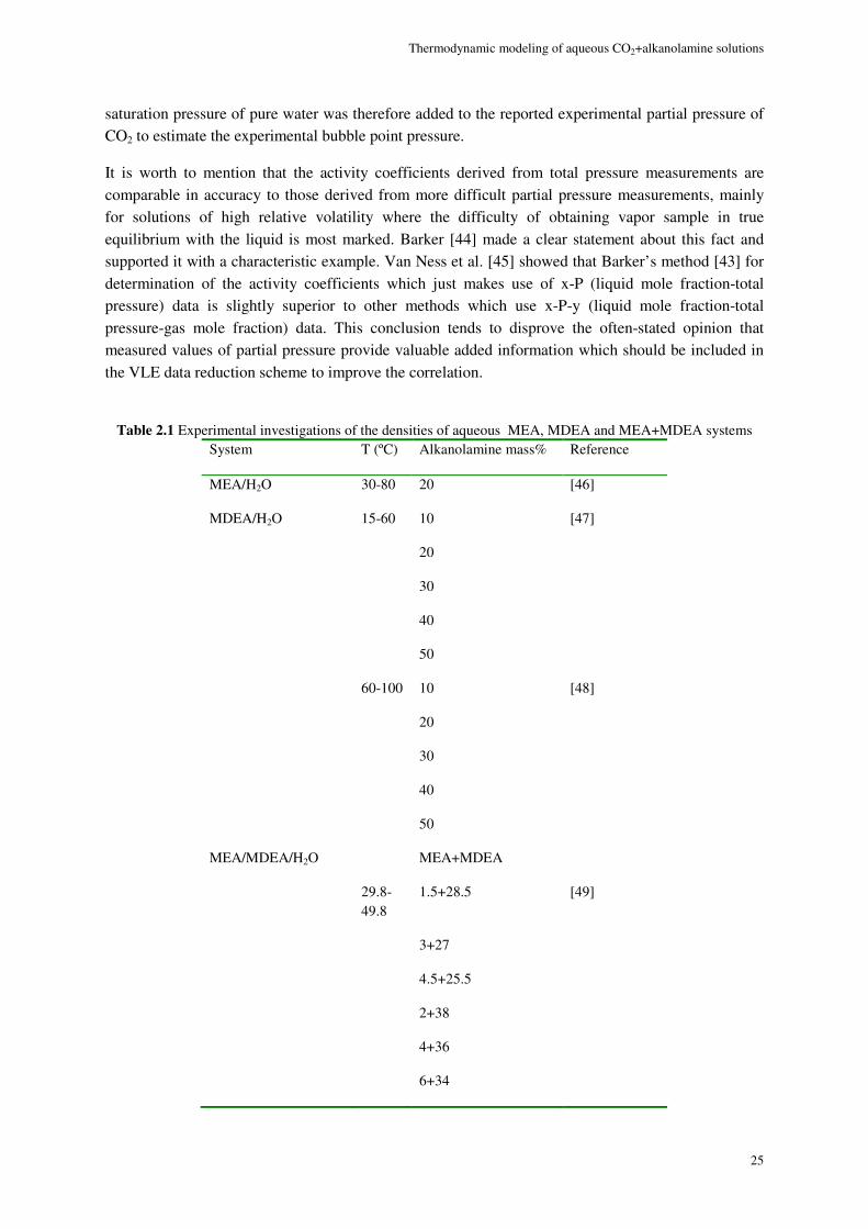
Thermodynamic modeling of aqueous CO2+alkanolamine solutions
25
saturation pressure of pure water was therefore added to the reported experimental partial pressure of CO2 to estimate the experimental bubble point pressure.
It is worth to mention that the activity coefficients derived from total pressure measurements are comparable in accuracy to those derived from more difficult partial pressure measurements, mainly for solutions of high relative volatility where the difficulty of obtaining vapor sample in true equilibrium with the liquid is most marked. Barker [44] made a clear statement about this fact and supported it with a characteristic example. Van Ness et al. [45] showed that Barker’s method [43] for determination of the activity coefficients which just makes use of x-P (liquid mole fraction-total pressure) data is slightly superior to other methods which use x-P-y (liquid mole fraction-total pressure-gas mole fraction) data. This conclusion tends to disprove the often-stated opinion that measured values of partial pressure provide valuable added information which should be included in the VLE data reduction scheme to improve the correlation.
Table 2.1 Experimental investigations of the densities of aqueous MEA, MDEA and MEA+MDEA systems
System T (ºC) Alkanolamine mass% Reference
MEA/H2O 30-80 20 [46]
MDEA/H2O 15-60 10 [47]
20
30
40
50
60-100 10 [48]
20
30
40
50
MEA/MDEA/H2O MEA+MDEA
29.8-49.8
1.5+28.5 [49]
3+27
4.5+25.5
2+38
4+36
6+34
CChhaapptteerr 22
26
Table 2.1 continued…
30-80
10+10
[50]
30-80 6+24 [46]
12+18
MEA/MDEA/H2O
MEA+MDEA
30-80 18+12 [46]
24+6
2.7.1. Data of aqueous alkanolamine solutions (alkanolamine-water)
Knowledge of the binary alkanolamine-water system can help with more confidently modeling the acid gas-alkanolamine-water system. This is especially the case for the solutions containing a small amount of CO2 where the composition of the system very much resembles that of the binary alkanolamine and water system.
Our search for the thermodynamic data on aqueous alkanolamine solutions revealed that, there are comparatively few data published on such systems. We have used H
E, VLE and freezing point depression data of alkanolamine-water solutions to tune the parameters of the model.
Binary VLE data are important in the determination of binary interaction parameters and also calculation of the loss of solvent due to vaporization. However, the available total pressure data can be more assuredly used at high temperatures and concentrated alkanolamine solutions. For the diluted solutions, freezing point depression can be measured more precisely than the pressure data and therefore, can be used with more confidence.
Like any other excess Gibbs energy model, extended UNIQUAC can benefit from being regressed to excess enthalpy data. Provided that the data of this type are of a good quality, they can help with better definition of the temperature dependence of the parameters.
The literature data on the VLE, freezing point depression and excess enthalpy of aqueous MEA system used in the thermodynamic modeling of this work are summarized in Table 2.2.
Binary VLE of MDEA-water system together with the freezing point depression and excess enthalpy of aqueous MDEA contribute 102 data-points to our thermodynamic properties databank. Table 2.3 summarizes the MDEA-water system data used in this work.
2.7.2. Data on solubility of CO2 in single alkanolamines (CO2-alkanolamine-water VLE data)
Perhaps the most important property for the design of the PCC unit based on alkanolamine absorption is the relationship between the concentration of CO2 in the solution and its partial pressure in the gas
Thermodynamic modeling of aqueous CO2+alkanolamine solutions
27
phase (VLE). The concentration in the liquid phase is dependent on the partial pressure of the acid gas, temperature, type of amine, amine strength and nature and concentration of other constituents of the solution.
Table 2.2 Data on the binary system of MEA+ water
Freezing point depression
Reference Temperature (ºC) MEA concentration (wt%)
[51] -4 -(-20) 9-35
VLE
Reference Temperature (ºC) MEA concentration (mole%)
[52] 88-170 (2 fixed pressures) 0-100
[53] 37-137 25, 50, 75
[54] 60, 78, 91.7 0-100
[55] 90 0-100
[56] 25, 35 0-100
Excess enthalpy
Reference Temperature (ºC) MEA concentration (mol%)
[56] 25 0.59-98
[57] 25 0.15-0.97
[58] 25, 69 15-67
Table 2.3 Data on the binary system of MDEA+ water
Freezing point depression
Reference Temperature (ºC) MDEA concentration (wt%)
[51] -3 -(-14) 32-58
VLE
Reference Pressure (kPa) MDEA concentration (wt%)
[59] 40.0, 53.3, 66.7 30-99
Excess enthalpy
Reference Temperature (ºC) MDEA concentration (wt%)
[60]
[61]
[58]
25, 40
65
25, 69.3
17-99
42-98
10-95
CChhaapptteerr 22
28
2.7.3. VLE measurement methods and associated errors
Generally, to experimentally determine the solubility of CO2 in alkanolamine solutions, there are two methods to approach equilibrium. One approach is the static method where a closed cell is used. The gas mixture is bubbled and recirculated through the liquid solvent. The sign of equilibrium in this method is when the pressure of the system does not vary anymore. In the second approach, the dynamic method, an open system is used with flow and continuous operation. The advantage of this method is that the gas can be analyzed without disturbing the equilibrium but the operation of the system is more difficult [62].
The experimental VLE data on solubility of CO2 in aqueous alkanolamine solutions are usually associated with errors. This can be the reason for the discrepancies among literature data.
Rumpf et al. [63] claim that the accuracy of the vapor pressure measurements is usually up to ±5%. Though, for the partial pressure measurements this can be as high as ±15% but typically 5-10% [64]. The sources of errors are varied and sometimes difficult to find out. The reason could be the measurement of equilibrium pressure or the errors due to determination of the pressure of the gas evolved form the liquid sample. Errors could also rise due to the titration methods for measuring acid gas loading and amine concentration. Rochelle et al. [62] claim that at high acid gas partial pressure, the techniques used to measure acid gas concentration in the liquid phase are the main sources of error. When the loading (mol CO2/mole alkanolamine) approaches one, the acid gas can flash easily from the liquid phase and this brings about difficulty in partial pressure measurements. Therefore, the major effort in acid gas solubility measurement is to avoid these problems.
Experimental data on solubility of CO2 in alkanolamine solutions are of vital importance for the thermodynamic modeling and design of PCC units based on reactive absorption. Therefore, the VLE data of aqueous mixtures of CO2 with single and blended alkanolamines were widely surveyed. A comprehensive database of the thermodynamic properties of some alkanolamine systems is made in this project. This includes solubility of acid gas in monoethanolamine (MEA), diethanolamine (DEA), N-methyldiethanolamine (MDEA), diglaycolamine (DGA), 2-amino-2-hydroxymethyl-1,3-propandiol (AHPD) and piperazine (PZ). The developed vapor-liquid equilibria (VLE) database covers a wide range of temperature, acid gas partial pressure and alkanolamine concentration.
Table 2.4 Ternary system of MEA+ water+ CO2
Reference Amine (wt%) Temperature (ºC) Loading
[67] 15.2 40, 60, 80, 120, 134, 140 0.11 - 0.99
[38] 6, 15.3, , 23.2, 31 24, 40, 60, 80, 100, 120 0.06 - 2.15
[37] 15.3 80, 100 0.03 - 0.28
[39] 15.3 25, 60, 80 0.41 - 1.32
[12] 15.3 40, 80 0.26 - 0.69
[68]
[65]
15.3, 30
12.2
40
30, 40, 50, 60, 70
0.22 - 1.04
0.46 - 0.91
Thermodynamic modeling of aqueous CO2+alkanolamine solutions
29
The VLE data of the MEA and MDEA systems have been screened and used for modeling.After analysis of the MEA and MDEA systems data, the datasets of Daneshvar et al. [65] and Shen and Li [68] both on the MEA system were excluded. The former, analyzed at different temperatures, showed internal (within the same dataset) as well as external (compared to others datasets) inconsistencies and the data from the latter source showed external inconsistency most notably at 100ºC. The high pressure MEA data of Jou et al. [66] were not used for tuning the model parameters either, as they were not consistent with all the other datasets at the same conditions.
Tables 2.4-2.8 summarize the references of the experimental data on the CO2-alkanolamine systems collected in the present project along with their measurement conditions.
Table 2.5 Literature review of CO2 solubility in aqueous DEA solutions Reference Amine (wt%) Temperature (ºC) CO2 Partial
Pressure (kPa) Loading
[38] 5.2, 21, 36.7, 52, 68, 84 0, 25, 50, 75, 100, 120, 140 0.68 - 6890 0.03 - 1.94
[67] 25 38, 66, 79, 93, 121 2 - 437 0.32 - 1.16
[39] 5.2, 21 25 6.28 - 2012 0.59 - 2.01
[69] 41.78 25, 75 0.34 - 4651 0.02 - 1.08
2.7.4. Data on solubility of CO2 in mixed alkanolamines (CO2-amine blend-water VLE data)
The open literature solubility data of aqueous blends of MEA-MDEA, DEA-MDEA and PZ-MDEA are collected. Table 2.9 presents the experimental VLE data on the quaternary systems of CO2 in double alkanolamine solutions. The data on the MEA-MDEA system are used for modeling and are presented together with the model representation in section 2.8.
Compared to single MEA/MDEA systems, there are few data available on the quaternary system of CO2-MEA-MDEA-water. Additionally, there is little overlap between the concentrations and temperatures the data from different sources cover. Therefore, a fair analysis was almost impossible and all the data available in the database were used in the regression process.
2.8. Results and discussion
The r and q parameters determined for MEA, MEAH+, MEA carbamate, MDEA and MDEAH+ are presented in Table 2.10. The best estimates for the interaction parameters are given in Table 2.11.
r and q for the rest of the species as well as the binary interaction parameters for the aqueous CO2 system (see section 2.2) are taken from Thomsen and Rasmussen [13].
The remaining 0ji
u parameters have been assigned a large value and their corresponding T
jiu
parameters are set to zero. The chosen default value for 0ji
u was large enough to eliminate the probable
effect on other parameters during the regression process. This was done for the pairs which were quite
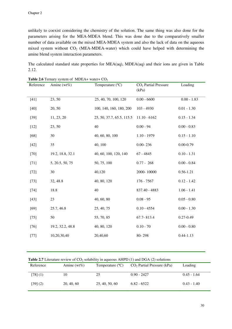
CChhaapptteerr 22
30
unlikely to coexist considering the chemistry of the solution. The same thing was also done for the parameters arising for the MEA-MDEA blend. This was done due to the comparatively smaller number of data available on the mixed MEA-MDEA system and also the lack of data on the aqueous mixed system without CO2 (MEA-MDEA-water) which could have helped with determining the amine blend system interaction parameters.
The calculated standard state properties for MEA(aq), MDEA(aq) and their ions are given in Table 2.12.
Table 2.6 Ternary system of MDEA+ water+ CO2
Reference Amine (wt%) Temperature (ºC) CO2 Partial Pressure (kPa)
Loading
[41] 23, 50 25, 40, 70, 100, 120 0.00 - 6600 0.00 - 1.83
[40] 20, 50 100, 140, 160, 180, 200 103 - 4930 0.01 - 1.30
[39] 11, 23, 20 25, 50, 37.7, 65.5, 115.5 11.10 - 6162 0.15 - 1.34
[12] 23, 50 40 0.00 - 94 0.00 - 0.83
[68] 30 40, 60, 80, 100 1.10 - 1979 0.15 - 1.10
[42] 35 40, 100 0.00- 236 0.00-0.79
[70] 19.2, 18.8, 32.1 40, 60, 100, 120, 140 67 - 4845 0.10 - 1.31
[71] 5, 20.5, 50, 75 50, 75, 100 0.77 - 268 0.00 - 0.84
[72] 30 40,120 2000- 10000 0.56-1.21
[73] 32, 48.8 40, 80, 120 176 - 7567 0.12 - 1.42
[74] 18.8 40 837.40 - 4883 1.06 - 1.41
[43] 23 40, 60, 80 0.08 - 95 0.05 - 0.80
[69] 25.7, 46.8 25, 40, 75 0.10 - 4554 0.00 - 1.30
[75] 50 55, 70, 85 67.7- 813.4 0.27-0.49
[76] 19.2, 32.2, 48.8 40, 80, 120 0.10 - 70 0.00 - 0.80
[77] 10,20,30,40 20,40,60 80- 298 0.44-1.13
Table 2.7 Literature review of CO2 solubility in aqueous AHPD (1) and DGA (2) solutions
Reference Amine (wt%) Temperature (ºC) CO2 Partial Pressure (kPa) Loading
[78] (1) 10 25 0.90 - 2427 0.45 - 1.64
[39] (2) 20, 40, 60 25, 40, 50, 60 6.82 - 6522 0.43 - 1.40
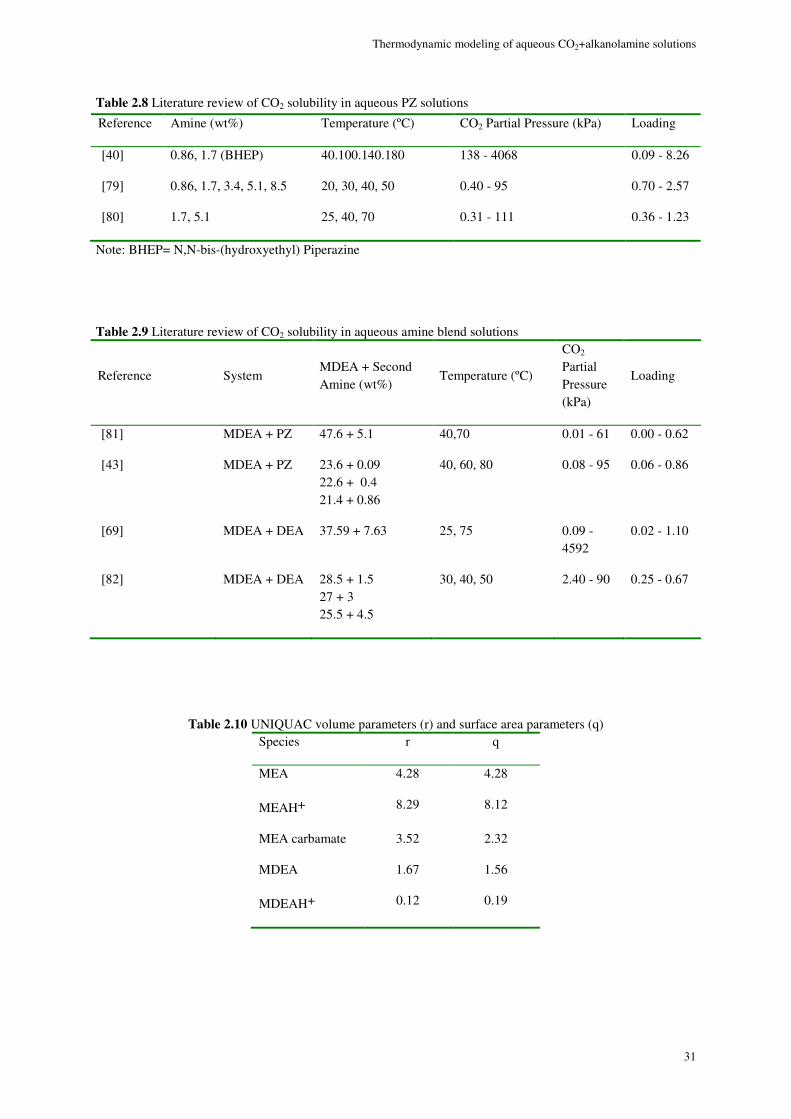
Thermodynamic modeling of aqueous CO2+alkanolamine solutions
31
Table 2.8 Literature review of CO2 solubility in aqueous PZ solutions
Reference Amine (wt%) Temperature (ºC) CO2 Partial Pressure (kPa) Loading
[40] 0.86, 1.7 (BHEP) 40.100.140.180 138 - 4068 0.09 - 8.26
[79] 0.86, 1.7, 3.4, 5.1, 8.5 20, 30, 40, 50 0.40 - 95 0.70 - 2.57
[80] 1.7, 5.1 25, 40, 70 0.31 - 111 0.36 - 1.23
Note: BHEP= N,N-bis-(hydroxyethyl) Piperazine
Table 2.9 Literature review of CO2 solubility in aqueous amine blend solutions
Reference System MDEA + Second Amine (wt%)
Temperature (ºC)
CO2 Partial Pressure (kPa)
Loading
[81] MDEA + PZ 47.6 + 5.1 40,70 0.01 - 61 0.00 - 0.62
[43] MDEA + PZ 23.6 + 0.09 22.6 + 0.4 21.4 + 0.86
40, 60, 80 0.08 - 95 0.06 - 0.86
[69] MDEA + DEA 37.59 + 7.63 25, 75 0.09 - 4592
0.02 - 1.10
[82] MDEA + DEA 28.5 + 1.5 27 + 3 25.5 + 4.5
30, 40, 50 2.40 - 90 0.25 - 0.67
Table 2.10 UNIQUAC volume parameters (r) and surface area parameters (q) Species r q
MEA 4.28 4.28
MEAH+ 8.29 8.12
MEA carbamate 3.52 2.32
MDEA 1.67 1.56
MDEAH+ 0.12 0.19
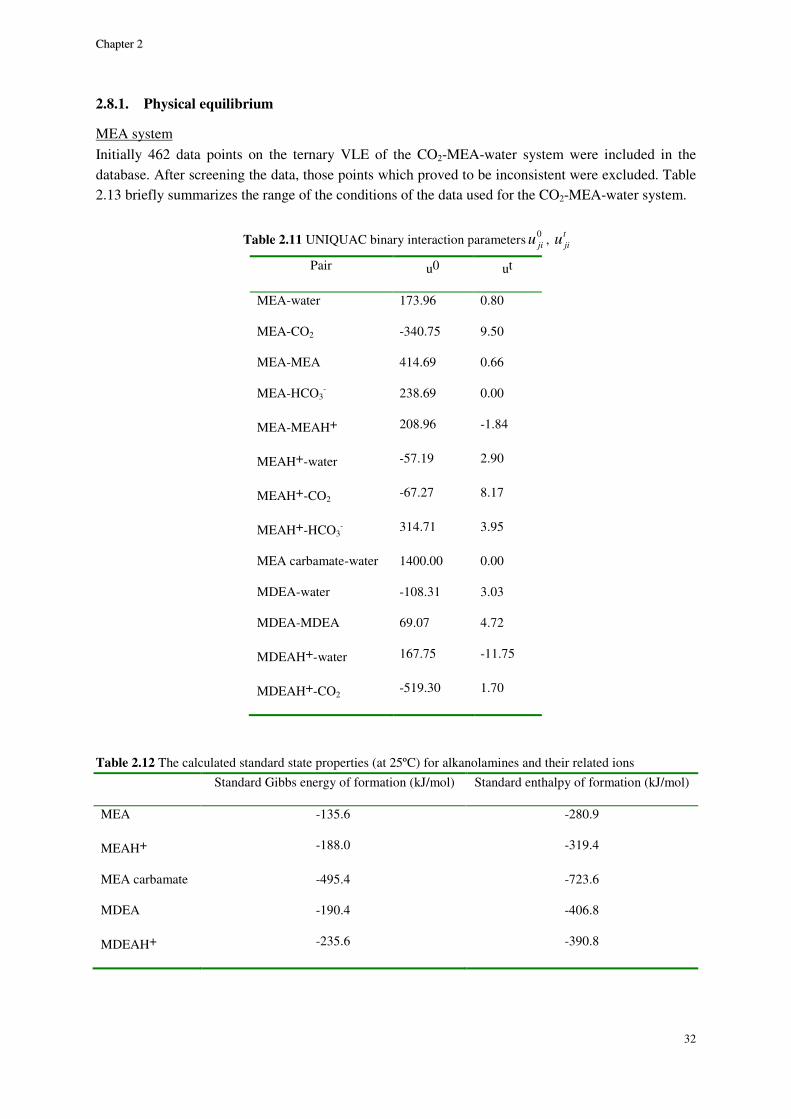
CChhaapptteerr 22
32
2.8.1. Physical equilibrium
MEA system Initially 462 data points on the ternary VLE of the CO2-MEA-water system were included in the database. After screening the data, those points which proved to be inconsistent were excluded. Table 2.13 briefly summarizes the range of the conditions of the data used for the CO2-MEA-water system.
Table 2.11 UNIQUAC binary interaction parameters 0ji
u , t
jiu
Pair u0 ut
MEA-water 173.96 0.80
MEA-CO2 -340.75 9.50
MEA-MEA 414.69 0.66
MEA-HCO3- 238.69 0.00
MEA-MEAH+ 208.96 -1.84
MEAH+-water -57.19 2.90
MEAH+-CO2 -67.27 8.17
MEAH+-HCO3- 314.71 3.95
MEA carbamate-water 1400.00 0.00
MDEA-water -108.31 3.03
MDEA-MDEA 69.07 4.72
MDEAH+-water 167.75 -11.75
MDEAH+-CO2 -519.30 1.70
Table 2.12 The calculated standard state properties (at 25ºC) for alkanolamines and their related ions
Standard Gibbs energy of formation (kJ/mol) Standard enthalpy of formation (kJ/mol)
MEA -135.6 -280.9
MEAH+ -188.0 -319.4
MEA carbamate -495.4 -723.6
MDEA -190.4 -406.8
MDEAH+ -235.6 -390.8
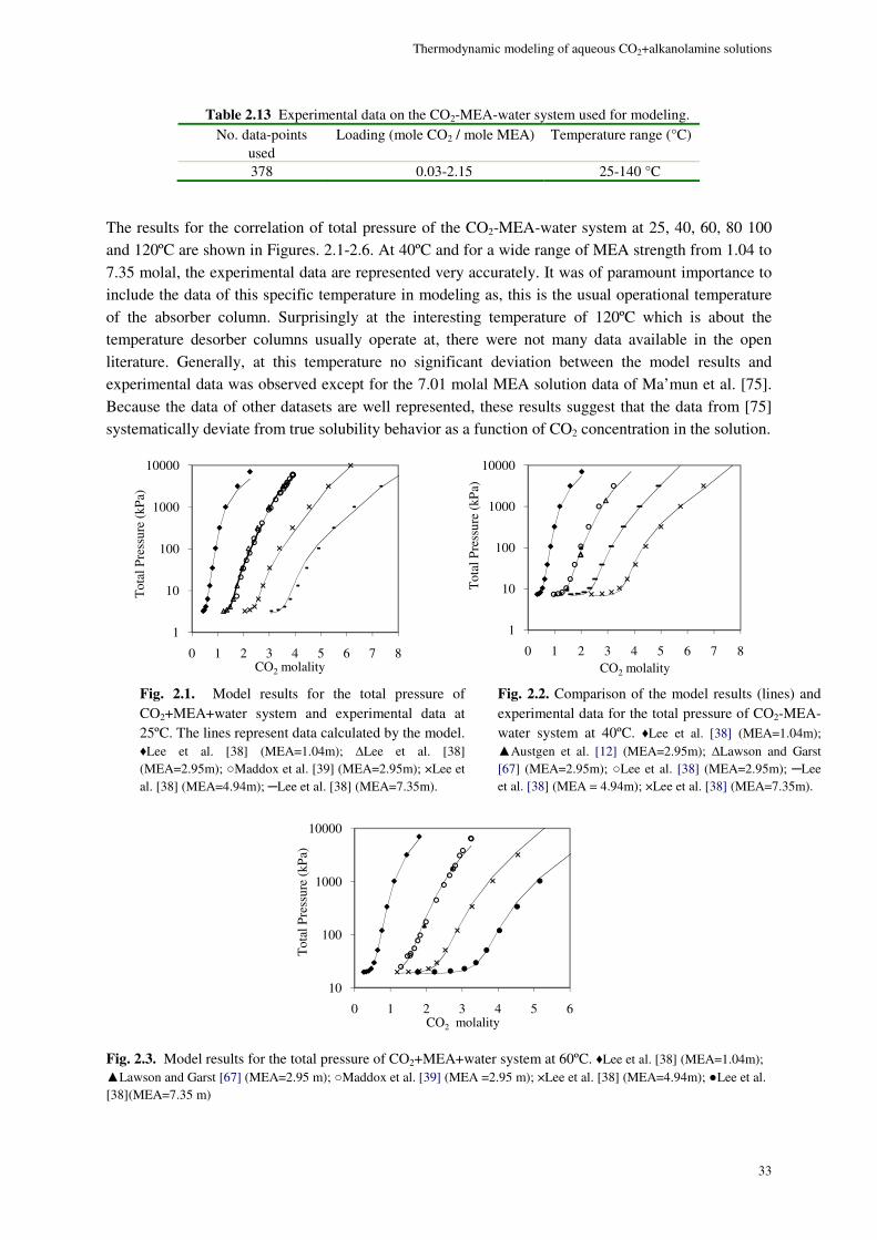
Thermodynamic modeling of aqueous CO2+alkanolamine solutions
33
Table 2.13 Experimental data on the CO2-MEA-water system used for modeling. No. data-points Loading (mole CO2 / mole MEA) Temperature range (°C)
used 378 0.03-2.15 25-140 °C
The results for the correlation of total pressure of the CO2-MEA-water system at 25, 40, 60, 80 100 and 120ºC are shown in Figures. 2.1-2.6. At 40ºC and for a wide range of MEA strength from 1.04 to 7.35 molal, the experimental data are represented very accurately. It was of paramount importance to include the data of this specific temperature in modeling as, this is the usual operational temperature of the absorber column. Surprisingly at the interesting temperature of 120ºC which is about the temperature desorber columns usually operate at, there were not many data available in the open literature. Generally, at this temperature no significant deviation between the model results and experimental data was observed except for the 7.01 molal MEA solution data of Ma’mun et al. [75]. Because the data of other datasets are well represented, these results suggest that the data from [75] systematically deviate from true solubility behavior as a function of CO2 concentration in the solution.
Fig. 2.3. Model results for the total pressure of CO2+MEA+water system at 60ºC. ♦Lee et al. [38] (MEA=1.04m); Lawson and Garst [67] (MEA=2.95 m); Maddox et al. [39] (MEA =2.95 m); ×Lee et al. [38] (MEA=4.94m); Lee et al. [38](MEA=7.35 m)
10
100
1000
10000
0 1 2 3 4 5 6
Tot
al P
ress
ure
(kP
a)
CO2 molality
1
10
100
1000
10000
0 1 2 3 4 5 6 7 8
Tot
al P
ress
ure
(kP
a)
CO2 molality
Fig. 2.1. Model results for the total pressure of CO2+MEA+water system and experimental data at 25ºC. The lines represent data calculated by the model. ♦Lee et al. [38] (MEA=1.04m); Lee et al. [38] (MEA=2.95m); Maddox et al. [39] (MEA=2.95m); ×Lee et al. [38] (MEA=4.94m); Lee et al. [38] (MEA=7.35m).
1
10
100
1000
10000
0 1 2 3 4 5 6 7 8
Tot
al P
ress
ure
(kP
a)
CO2 molality
Fig. 2.2. Comparison of the model results (lines) and experimental data for the total pressure of CO2-MEA- water system at 40ºC. ♦Lee et al. [38] (MEA=1.04m); Austgen et al. [12] (MEA=2.95m); Lawson and Garst [67] (MEA=2.95m); Lee et al. [38] (MEA=2.95m); Lee et al. [38] (MEA = 4.94m); ×Lee et al. [38] (MEA=7.35m).
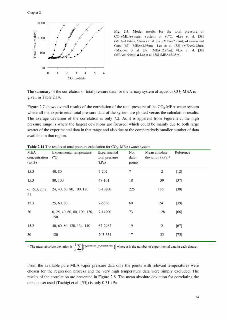
CChhaapptteerr 22
34
The summary of the correlation of total pressure data for the ternary system of aqueous CO2-MEA is given in Table 2.14.
Figure 2.7 shows overall results of the correlation of the total pressure of the CO2-MEA-water system where all the experimental total pressure data of the system are plotted versus the calculation results. The average deviation of the correlation is only 7.2. As it is apparent from Figure 2.7, the high pressure range is where the largest deviations are focused, which could be mainly due to both large scatter of the experimental data in that range and also due to the comparatively smaller number of data available in that region. Table 2.14 The results of total pressure calculation for CO2+MEA+water system
MEA concentration (wt%)
Experimental temperature (ºC)
Experimental total pressure (kPa)
No. data-points
Mean absolute deviation (kPa)*
Reference
15.3 40, 80 7-202 7 2 [12]
15.3 80, 100 47-101 18 39 [37]
6, 15.3, 23.2, 31
24, 40, 60, 80, 100, 120 3-10200 225 186 [38]
15.3 25, 60, 80 7-6836 60 241 [39]
30 0, 25, 40, 60, 80, 100, 120, 150
7-14900 73 128 [66]
15.2 40, 60, 80, 120, 134, 140 67-2982 19 2 [67]
30 120 203-334 17 33 [75]
* The mean absolute deviation is ( )calculated experimental
i=n
1P -P
n∑ where n is the number of experimental data in each dataset.
From the available pure MEA vapor pressure data only the points with relevant temperatures were chosen for the regression process and the very high temperature data were simply excluded. The results of the correlation are presented in Figure 2.8. The mean absolute deviation for correlating the one dataset used (Tochigi et al. [55]) is only 0.31 kPa.
Fig. 2.4. Model results for the total pressure of CO2+MEA+water system at 80ºC. ♦Lee et al. [38] (MEA=1.04m); Isaacs et al. [37] (MEA=2.95m); Lawson and Garst [67] (MEA=2.95m); +Lee et al. [38] (MEA=2.95m); Maddox et al. [39] (MEA=2.95m); ◊Lee et al. [38] (MEA=4.94m); Lee et al. [38] (MEA=7.35m).
10
100
1000
10000
0 1 2 3 4 5 6
Tot
al P
ress
ure
(kP
a)
CO2 molality
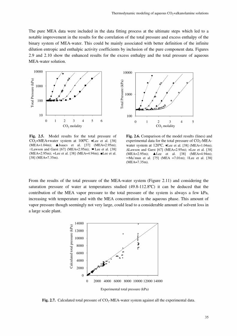
Thermodynamic modeling of aqueous CO2+alkanolamine solutions
35
The pure MEA data were included in the data fitting process at the ultimate steps which led to a notable improvement in the results for the correlation of the total pressure and excess enthalpy of the binary system of MEA-water. This could be mainly associated with better definition of the infinite dilution entropic and enthalpic activity coefficients by inclusion of the pure component data. Figures 2.9 and 2.10 show the enhanced results for the excess enthalpy and the total pressure of aqueous MEA-water solution.
From the results of the total pressure of the MEA-water system (Figure 2.11) and considering the saturation pressure of water at temperatures studied (49.8-112.8ºC) it can be deduced that the contribution of the MEA vapor pressure to the total pressure of the system is always a few kPa, increasing with temperature and with the MEA concentration in the aqueous phase. This amount of vapor pressure though seemingly not very large, could lead to a considerable amount of solvent loss in a large scale plant.
Fig. 2.7. Calculated total pressure of CO2-MEA-water system against all the experimental data.
0
2000
4000
6000
8000
10000
12000
14000
0 2000 4000 6000 8000 10000 12000 14000
Cal
cula
ted
tota
l pre
ssur
e (k
Pa)
Experimental total pressure (kPa)
10
100
1000
10000
0 1 2 3 4 5 6
Tot
al P
ress
ure
(kP
a)
CO2 molality
Fig. 2.5. Model results for the total pressure of CO2+MEA+water system at 100ºC. ♦Lee et al. [38] (MEA=1.04m); Isaacs et al. [37] (MEA=2.95m); Lawson and Garst [67] (MEA=2.95m); Lee et al. [38] (MEA=2.95m); +Lee et al. [38] (MEA=4.94m); Lee et al. [38] (MEA=7.35m).
100
1000
10000
0 1 2 3 4 5T
otal
Pre
ssur
e (k
Pa)
CO2 molality
Fig. 2.6. Comparison of the model results (lines) and experimental data for the total pressure of CO2-MEA-water system at 120ºC. ♦Lee et al. [38] (MEA=1.04m); Lawson and Garst [67] (MEA=2.95m); ×Lee et al. [38] (MEA=2.95m); Lee et al. [38] (MEA=4.94m); Ma’mun et al. [75] (MEA =7.01m); ◊Lee et al. [38] (MEA=7.35m).
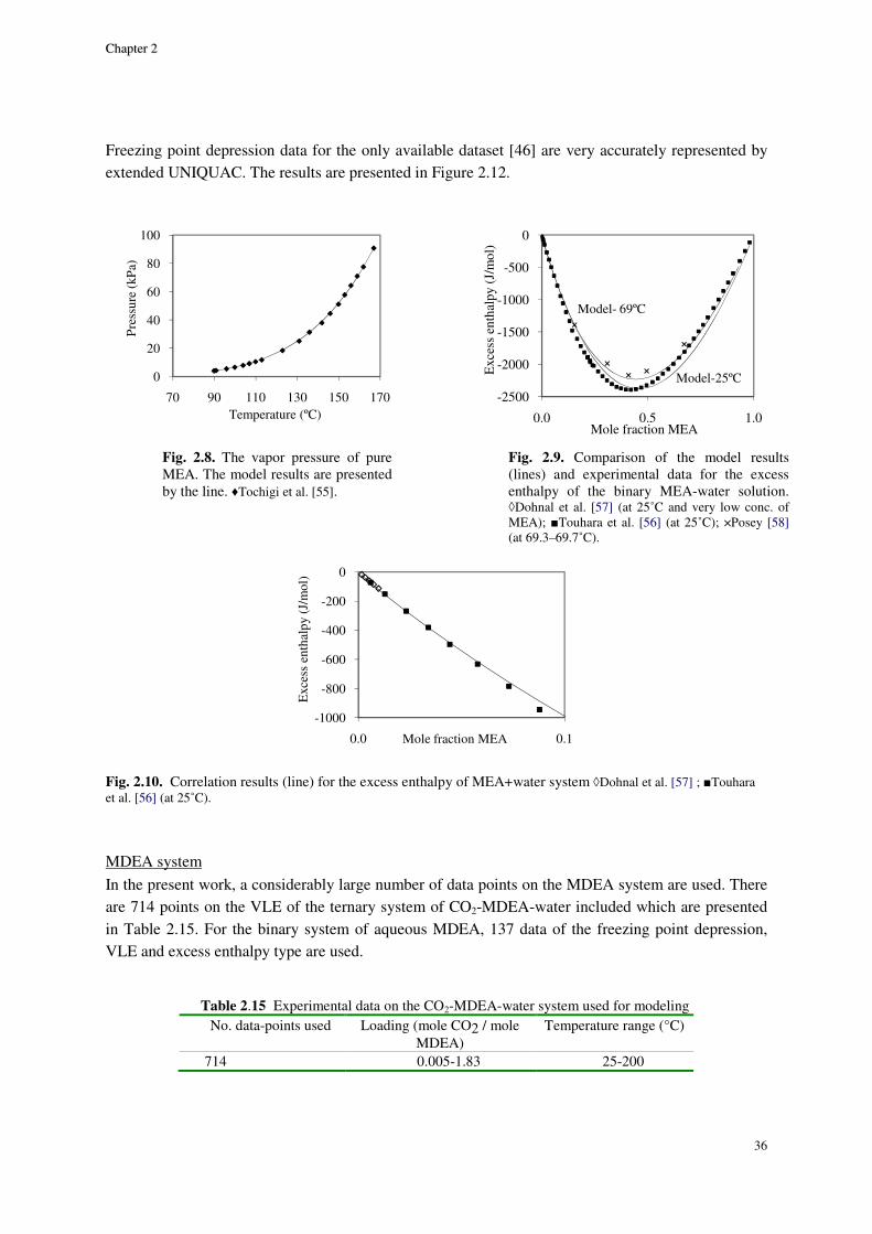
CChhaapptteerr 22
36
Freezing point depression data for the only available dataset [46] are very accurately represented by extended UNIQUAC. The results are presented in Figure 2.12.
Fig. 2.10. Correlation results (line) for the excess enthalpy of MEA+water system ◊Dohnal et al. [57] ; Touhara et al. [56] (at 25˚C).
MDEA system
In the present work, a considerably large number of data points on the MDEA system are used. There are 714 points on the VLE of the ternary system of CO2-MDEA-water included which are presented in Table 2.15. For the binary system of aqueous MDEA, 137 data of the freezing point depression, VLE and excess enthalpy type are used.
Table 2.15 Experimental data on the CO2-MDEA-water system used for modeling No. data-points used Loading (mole CO2 / mole
MDEA) Temperature range (°C)
714 0.005-1.83 25-200
-1000
-800
-600
-400
-200
0
0.0 0.1
Exc
ess
enth
alpy
(J/
mol
)
Mole fraction MEA
Fig. 2.8. The vapor pressure of pure MEA. The model results are presented by the line. ♦Tochigi et al. [55].
-2500
-2000
-1500
-1000
-500
0
0.0 0.5 1.0
Exc
ess
enth
alpy
(J/
mol
)
Mole fraction MEA
Model-25ºC
Model- 69ºC
Fig. 2.9. Comparison of the model results (lines) and experimental data for the excess enthalpy of the binary MEA-water solution. ◊Dohnal et al. [57] (at 25˚C and very low conc. of MEA); Touhara et al. [56] (at 25˚C); ×Posey [58] (at 69.3–69.7˚C).
0
20
40
60
80
100
70 90 110 130 150 170
Pre
ssur
e (k
Pa)
Temperature (ºC)
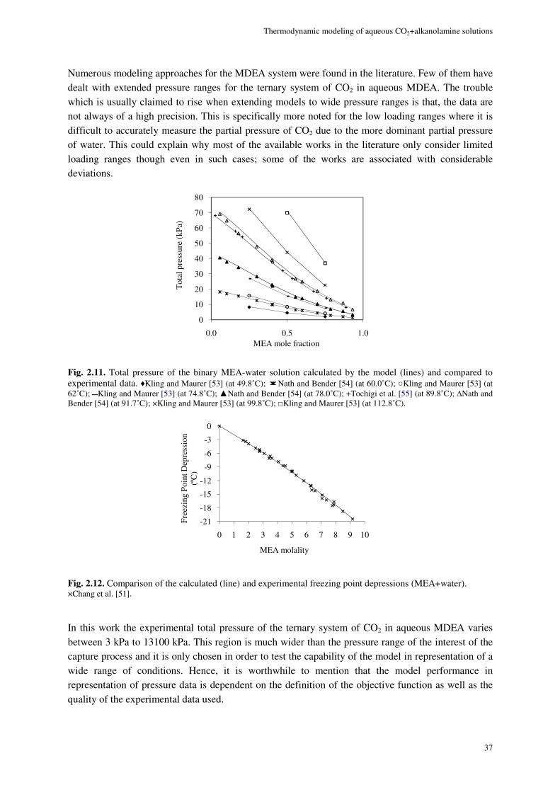
Thermodynamic modeling of aqueous CO2+alkanolamine solutions
37
Numerous modeling approaches for the MDEA system were found in the literature. Few of them have dealt with extended pressure ranges for the ternary system of CO2 in aqueous MDEA. The trouble which is usually claimed to rise when extending models to wide pressure ranges is that, the data are not always of a high precision. This is specifically more noted for the low loading ranges where it is difficult to accurately measure the partial pressure of CO2 due to the more dominant partial pressure of water. This could explain why most of the available works in the literature only consider limited loading ranges though even in such cases; some of the works are associated with considerable deviations.
Fig. 2.11. Total pressure of the binary MEA-water solution calculated by the model (lines) and compared to experimental data. ♦Kling and Maurer [53] (at 49.8˚C); Nath and Bender [54] (at 60.0˚C); Kling and Maurer [53] (at 62˚C); Kling and Maurer [53] (at 74.8˚C); Nath and Bender [54] (at 78.0˚C); +Tochigi et al. [55] (at 89.8˚C); Nath and Bender [54] (at 91.7˚C); ×Kling and Maurer [53] (at 99.8˚C); Kling and Maurer [53] (at 112.8˚C).
Fig. 2.12. Comparison of the calculated (line) and experimental freezing point depressions (MEA+water). ×Chang et al. [51].
In this work the experimental total pressure of the ternary system of CO2 in aqueous MDEA varies between 3 kPa to 13100 kPa. This region is much wider than the pressure range of the interest of the capture process and it is only chosen in order to test the capability of the model in representation of a wide range of conditions. Hence, it is worthwhile to mention that the model performance in representation of pressure data is dependent on the definition of the objective function as well as the quality of the experimental data used.
0
10
20
30
40
50
60
70
80
0.0 0.5 1.0
Tot
al p
ress
ure
(kP
a)
MEA mole fraction
-21
-18
-15
-12
-9
-6
-3
0
0 1 2 3 4 5 6 7 8 9 10
Free
zing
Poi
nt D
epre
ssio
n (º
C)
MEA molality
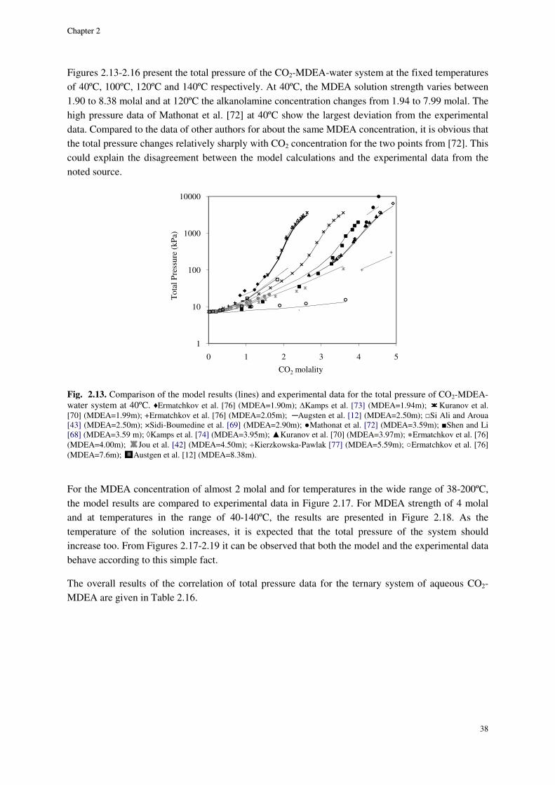
CChhaapptteerr 22
38
Figures 2.13-2.16 present the total pressure of the CO2-MDEA-water system at the fixed temperatures of 40ºC, 100ºC, 120ºC and 140ºC respectively. At 40ºC, the MDEA solution strength varies between 1.90 to 8.38 molal and at 120ºC the alkanolamine concentration changes from 1.94 to 7.99 molal. The high pressure data of Mathonat et al. [72] at 40ºC show the largest deviation from the experimental data. Compared to the data of other authors for about the same MDEA concentration, it is obvious that the total pressure changes relatively sharply with CO2 concentration for the two points from [72]. This could explain the disagreement between the model calculations and the experimental data from the noted source.
Fig. 2.13. Comparison of the model results (lines) and experimental data for the total pressure of CO2-MDEA-water system at 40ºC. ♦Ermatchkov et al. [76] (MDEA=1.90m); Kamps et al. [73] (MDEA=1.94m); Kuranov et al. [70] (MDEA=1.99m); +Ermatchkov et al. [76] (MDEA=2.05m); Augsten et al. [12] (MDEA=2.50m); Si Ali and Aroua [43] (MDEA=2.50m); ×Sidi-Boumedine et al. [69] (MDEA=2.90m); Mathonat et al. [72] (MDEA=3.59m); Shen and Li [68] (MDEA=3.59 m); ◊Kamps et al. [74] (MDEA=3.95m); Kuranov et al. [70] (MDEA=3.97m); Ermatchkov et al. [76] (MDEA=4.00m); Jou et al. [42] (MDEA=4.50m); +Kierzkowska-Pawlak [77] (MDEA=5.59m); Ermatchkov et al. [76] (MDEA=7.6m); Austgen et al. [12] (MDEA=8.38m).
For the MDEA concentration of almost 2 molal and for temperatures in the wide range of 38-200ºC, the model results are compared to experimental data in Figure 2.17. For MDEA strength of 4 molal and at temperatures in the range of 40-140ºC, the results are presented in Figure 2.18. As the temperature of the solution increases, it is expected that the total pressure of the system should increase too. From Figures 2.17-2.19 it can be observed that both the model and the experimental data behave according to this simple fact.
The overall results of the correlation of total pressure data for the ternary system of aqueous CO2-MDEA are given in Table 2.16.
1
10
100
1000
10000
0 1 2 3 4 5
Tot
al P
ress
ure
(kP
a)
CO2 molality
`
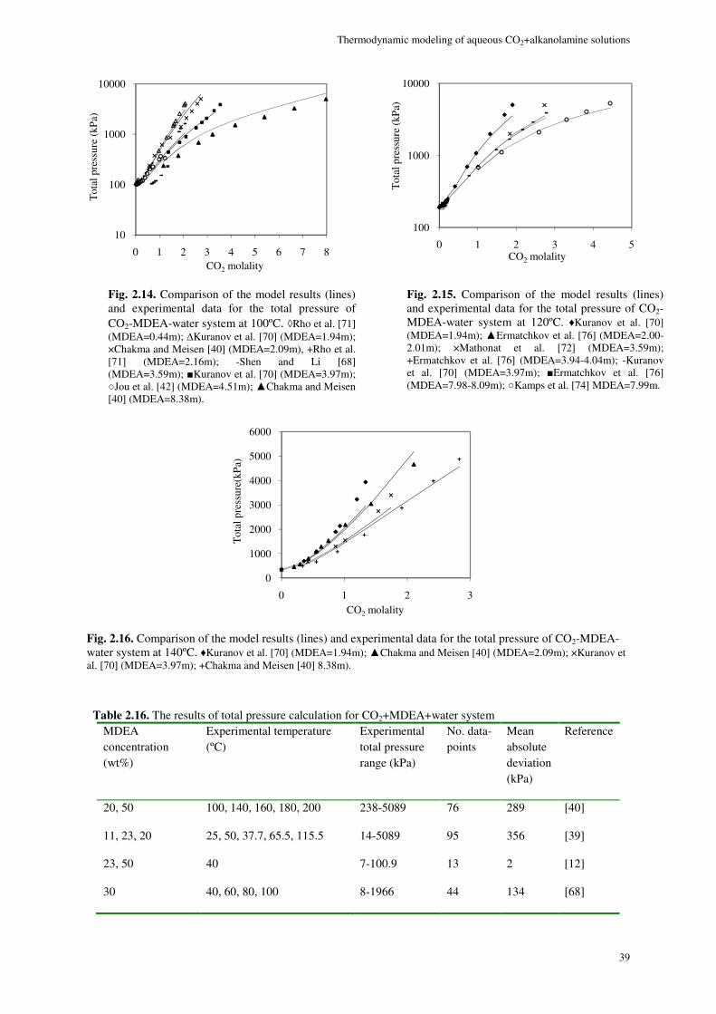
Thermodynamic modeling of aqueous CO2+alkanolamine solutions
39
Fig. 2.16. Comparison of the model results (lines) and experimental data for the total pressure of CO2-MDEA-water system at 140ºC. ♦Kuranov et al. [70] (MDEA=1.94m); Chakma and Meisen [40] (MDEA=2.09m); ×Kuranov et al. [70] (MDEA=3.97m); +Chakma and Meisen [40] 8.38m).
Table 2.16. The results of total pressure calculation for CO2+MDEA+water system MDEA concentration (wt%)
Experimental temperature (ºC)
Experimental total pressure range (kPa)
No. data-points
Mean absolute deviation (kPa)
Reference
20, 50 100, 140, 160, 180, 200 238-5089 76 289 [40]
11, 23, 20 25, 50, 37.7, 65.5, 115.5 14-5089 95 356 [39]
23, 50 40 7-100.9 13 2 [12]
30 40, 60, 80, 100 8-1966 44 134 [68]
0
1000
2000
3000
4000
5000
6000
0 1 2 3
Tot
al p
ress
ure(
kPa)
CO2 molality
10
100
1000
10000
0 1 2 3 4 5 6 7 8
Tot
al p
ress
ure
(kP
a)
CO2 molality
100
1000
10000
0 1 2 3 4 5
Tot
al p
ress
ure
(kP
a)
CO2 molality
Fig. 2.14. Comparison of the model results (lines) and experimental data for the total pressure of CO2-MDEA-water system at 100ºC. ◊Rho et al. [71] (MDEA=0.44m); Kuranov et al. [70] (MDEA=1.94m); ×Chakma and Meisen [40] (MDEA=2.09m), +Rho et al. [71] (MDEA=2.16m); -Shen and Li [68] (MDEA=3.59m); Kuranov et al. [70] (MDEA=3.97m); Jou et al. [42] (MDEA=4.51m); Chakma and Meisen [40] (MDEA=8.38m).
Fig. 2.15. Comparison of the model results (lines) and experimental data for the total pressure of CO2-MDEA-water system at 120ºC. ♦Kuranov et al. [70] (MDEA=1.94m); Ermatchkov et al. [76] (MDEA=2.00-2.01m); ×Mathonat et al. [72] (MDEA=3.59m); +Ermatchkov et al. [76] (MDEA=3.94-4.04m); -Kuranov et al. [70] (MDEA=3.97m); Ermatchkov et al. [76] (MDEA=7.98-8.09m); Kamps et al. [74] MDEA=7.99m.
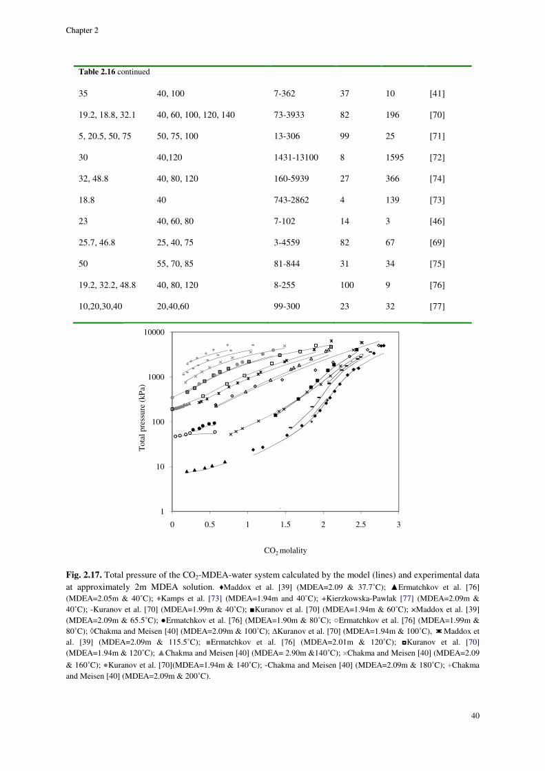
CChhaapptteerr 22
40
Table 2.16 continued
35 40, 100 7-362 37 10 [41]
19.2, 18.8, 32.1 40, 60, 100, 120, 140 73-3933 82 196 [70]
5, 20.5, 50, 75 50, 75, 100 13-306 99 25 [71]
30 40,120 1431-13100 8 1595 [72]
32, 48.8 40, 80, 120 160-5939 27 366 [74]
18.8 40 743-2862 4 139 [73]
23 40, 60, 80 7-102 14 3 [46]
25.7, 46.8 25, 40, 75 3-4559 82 67 [69]
50 55, 70, 85 81-844 31 34 [75]
19.2, 32.2, 48.8 40, 80, 120 8-255 100 9 [76]
10,20,30,40 20,40,60 99-300 23 32 [77]
Fig. 2.17. Total pressure of the CO2-MDEA-water system calculated by the model (lines) and experimental data at approximately 2m MDEA solution. ♦Maddox et al. [39] (MDEA=2.09 & 37.7˚C); Ermatchkov et al. [76] (MDEA=2.05m & 40˚C); ♦Kamps et al. [73] (MDEA=1.94m and 40˚C); +Kierzkowska-Pawlak [77] (MDEA=2.09m & 40˚C); -Kuranov et al. [70] (MDEA=1.99m & 40˚C); Kuranov et al. [70] (MDEA=1.94m & 60˚C); ×Maddox et al. [39] (MDEA=2.09m & 65.5˚C); Ermatchkov et al. [76] (MDEA=1.90m & 80˚C); Ermatchkov et al. [76] (MDEA=1.99m & 80˚C); ◊Chakma and Meisen [40] (MDEA=2.09m & 100˚C); Kuranov et al. [70] (MDEA=1.94m & 100˚C), Maddox et al. [39] (MDEA=2.09m & 115.5˚C); Ermatchkov et al. [76] (MDEA=2.01m & 120˚C); Kuranov et al. [70] (MDEA=1.94m & 120˚C); Chakma and Meisen [40] (MDEA= 2.90m &140˚C); ×Chakma and Meisen [40] (MDEA=2.09
& 160˚C); Kuranov et al. [70](MDEA=1.94m & 140˚C); -Chakma and Meisen [40] (MDEA=2.09m & 180˚C); +Chakma and Meisen [40] (MDEA=2.09m & 200˚C).
1
10
100
1000
10000
0 0.5 1 1.5 2 2.5 3
Tot
al p
ress
ure
(kP
a)
CO2 molality
z
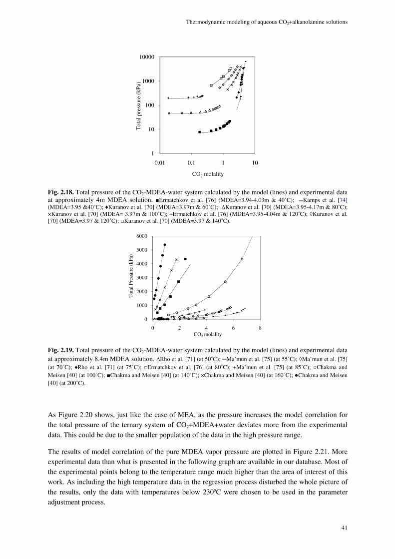
Thermodynamic modeling of aqueous CO2+alkanolamine solutions
41
Fig. 2.18. Total pressure of the CO2-MDEA-water system calculated by the model (lines) and experimental data at approximately 4m MDEA solution. Ermatchkov et al. [76] (MDEA=3.94-4.03m & 40˚C); Kamps et al. [74] (MDEA=3.95 &40˚C); ♦Kuranov et al. [70] (MDEA=3.97m & 60˚C); Kuranov et al. [70] (MDEA=3.95-4.17m & 80˚C); ×Kuranov et al. [70] (MDEA= 3.97m & 100˚C); +Ermatchkov et al. [76] (MDEA=3.95-4.04m & 120˚C); ◊Kuranov et al. [70] (MDEA=3.97 & 120˚C); Kuranov et al. [70] (MDEA=3.97 & 140˚C).
Fig. 2.19. Total pressure of the CO2-MDEA-water system calculated by the model (lines) and experimental data at approximately 8.4m MDEA solution. Rho et al. [71] (at 50˚C); Ma’mun et al. [75] (at 55˚C); ◊Ma’mun et al. [75] (at 70˚C); ♦Rho et al. [71] (at 75˚C); Ermatchkov et al. [76] (at 80˚C); +Ma’mun et al. [75] (at 85˚C); Chakma and Meisen [40] (at 100˚C); Chakma and Meisen [40] (at 140˚C); ×Chakma and Meisen [40] (at 160˚C); Chakma and Meisen [40] (at 200˚C).
As Figure 2.20 shows, just like the case of MEA, as the pressure increases the model correlation for the total pressure of the ternary system of CO2+MDEA+water deviates more from the experimental data. This could be due to the smaller population of the data in the high pressure range.
The results of model correlation of the pure MDEA vapor pressure are plotted in Figure 2.21. More experimental data than what is presented in the following graph are available in our database. Most of the experimental points belong to the temperature range much higher than the area of interest of this work. As including the high temperature data in the regression process disturbed the whole picture of the results, only the data with temperatures below 230ºC were chosen to be used in the parameter adjustment process.
1
10
100
1000
10000
0.01 0.1 1 10
Tot
al p
ress
ure
(kP
a)
CO2 molality
0
1000
2000
3000
4000
5000
6000
0 2 4 6 8
Tot
al P
ress
ure
(kPa
)
CO2 molality
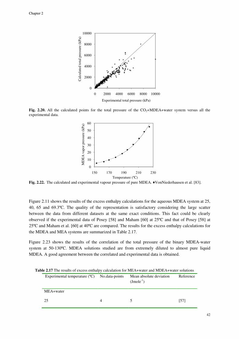
CChhaapptteerr 22
42
Fig. 2.20. All the calculated points for the total pressure of the CO2+MDEA+water system versus all the experimental data.
Fig. 2.22. The calculated and experimental vapour pressure of pure MDEA. ♦VonNiederhausen et al. [83].
Figure 2.11 shows the results of the excess enthalpy calculations for the aqueous MDEA system at 25, 40, 65 and 69.3ºC. The quality of the representation is satisfactory considering the large scatter between the data from different datasets at the same exact conditions. This fact could be clearly observed if the experimental data of Posey [58] and Maham [60] at 25ºC and that of Posey [58] at 25ºC and Maham et al. [60] at 40ºC are compared. The results for the excess enthalpy calculations for the MDEA and MEA systems are summarized in Table 2.17.
Figure 2.23 shows the results of the correlation of the total pressure of the binary MDEA-water system at 50-130ºC. MDEA solutions studied are from extremely diluted to almost pure liquid MDEA. A good agreement between the correlated and experimental data is obtained.
Table 2.17 The results of excess enthalpy calculation for MEA+water and MDEA+water solutions
Experimental temperature (ºC) No.data-points Mean absolute deviation (Jmole-1)
Reference
MEA+water
25 4 5 [57]
0
2000
4000
6000
8000
10000
0 2000 4000 6000 8000 10000
Cal
cula
ted
tota
l pre
ssur
e (k
Pa)
Experimental total pressure (kPa)
0
10
20
30
40
50
60
150 170 190 210 230
MD
EA
vap
or p
ress
ure
(kP
a)
Temperature (ºC)
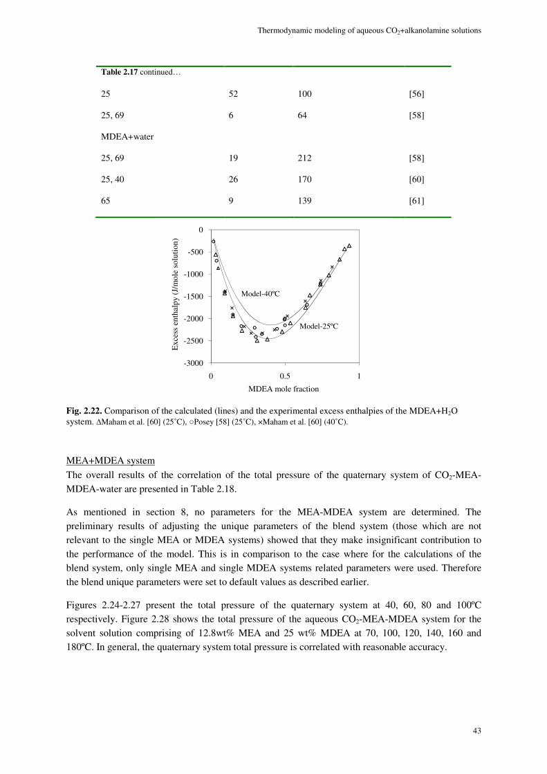
Thermodynamic modeling of aqueous CO2+alkanolamine solutions
43
Table 2.17 continued…
25 52 100 [56]
25, 69 6 64 [58]
MDEA+water
25, 69 19 212 [58]
25, 40 26 170 [60]
65 9 139 [61]
Fig. 2.22. Comparison of the calculated (lines) and the experimental excess enthalpies of the MDEA+H2O system. Maham et al. [60] (25˚C), Posey [58] (25˚C), ×Maham et al. [60] (40˚C).
MEA+MDEA system The overall results of the correlation of the total pressure of the quaternary system of CO2-MEA-MDEA-water are presented in Table 2.18.
As mentioned in section 8, no parameters for the MEA-MDEA system are determined. The preliminary results of adjusting the unique parameters of the blend system (those which are not relevant to the single MEA or MDEA systems) showed that they make insignificant contribution to the performance of the model. This is in comparison to the case where for the calculations of the blend system, only single MEA and single MDEA systems related parameters were used. Therefore the blend unique parameters were set to default values as described earlier.
Figures 2.24-2.27 present the total pressure of the quaternary system at 40, 60, 80 and 100ºC respectively. Figure 2.28 shows the total pressure of the aqueous CO2-MEA-MDEA system for the solvent solution comprising of 12.8wt% MEA and 25 wt% MDEA at 70, 100, 120, 140, 160 and 180ºC. In general, the quaternary system total pressure is correlated with reasonable accuracy.
-3000
-2500
-2000
-1500
-1000
-500
0
0 0.5 1
Exc
ess
enth
alpy
(J/
mol
e so
lutio
n)
MDEA mole fraction
Model-25ºC
Model-40ºC
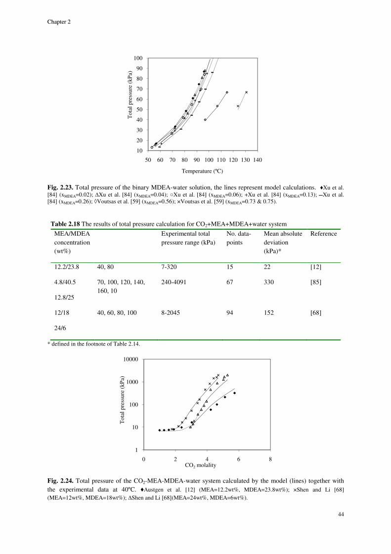
CChhaapptteerr 22
44
Fig. 2.23. Total pressure of the binary MDEA-water solution, the lines represent model calculations. ♦Xu et al. [84] (xMDEA=0.02); Xu et al. [84] (xMDEA=0.04); Xu et al. [84] (xMDEA=0.06); +Xu et al. [84] (xMDEA=0.13); Xu et al. [84] (xMDEA=0.26); ◊Voutsas et al. [59] (xMDEA=0.56); ×Voutsas et al. [59] (xMDEA=0.73 & 0.75).
Table 2.18 The results of total pressure calculation for CO2+MEA+MDEA+water system
MEA/MDEA concentration (wt%)
Experimental total pressure range (kPa)
No. data-points
Mean absolute deviation (kPa)*
Reference
12.2/23.8 40, 80 7-320 15 22 [12]
4.8/40.5
12.8/25
70, 100, 120, 140, 160, 10
240-4091 67 330 [85]
12/18
24/6
40, 60, 80, 100 8-2045 94 152 [68]
* defined in the footnote of Table 2.14.
Fig. 2.24. Total pressure of the CO2-MEA-MDEA-water system calculated by the model (lines) together with the experimental data at 40ºC. ♦Austgen et al. [12] (MEA=12.2wt%, MDEA=23.8wt%); ×Shen and Li [68] (MEA=12wt%, MDEA=18wt%); Shen and Li [68](MEA=24wt%, MDEA=6wt%).
10
20
30
40
50
60
70
80
90
100
50 60 70 80 90 100 110 120 130 140
Tot
al p
ress
ure
(kP
a)
Temperature (ºC)
1
10
100
1000
10000
0 2 4 6 8
Tot
al p
ress
ure
(kP
a)
CO2 molality
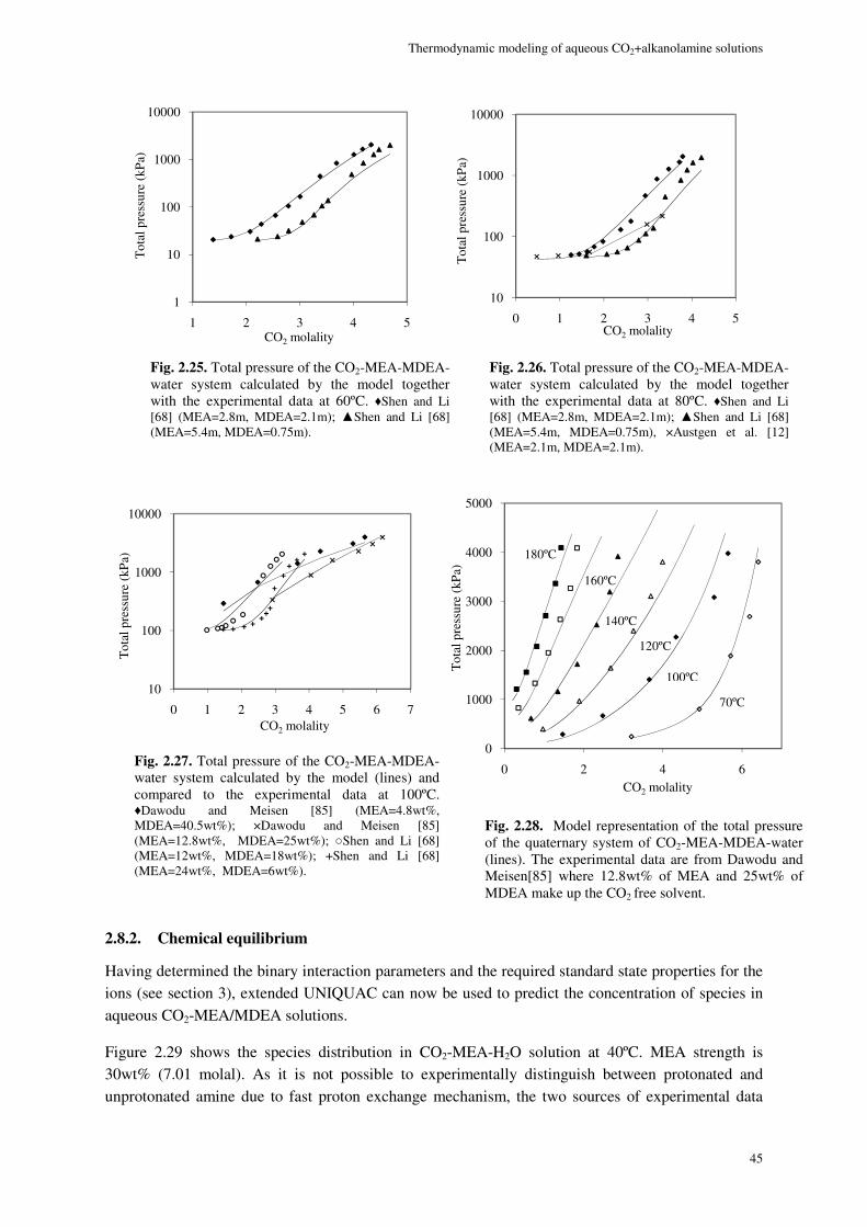
Thermodynamic modeling of aqueous CO2+alkanolamine solutions
45
2.8.2. Chemical equilibrium
Having determined the binary interaction parameters and the required standard state properties for the ions (see section 3), extended UNIQUAC can now be used to predict the concentration of species in aqueous CO2-MEA/MDEA solutions.
Figure 2.29 shows the species distribution in CO2-MEA-H2O solution at 40ºC. MEA strength is 30wt% (7.01 molal). As it is not possible to experimentally distinguish between protonated and unprotonated amine due to fast proton exchange mechanism, the two sources of experimental data
1
10
100
1000
10000
1 2 3 4 5
Tot
al p
ress
ure
(kP
a)
CO2 molality
Fig. 2.25. Total pressure of the CO2-MEA-MDEA-water system calculated by the model together with the experimental data at 60ºC. ♦Shen and Li [68] (MEA=2.8m, MDEA=2.1m); Shen and Li [68] (MEA=5.4m, MDEA=0.75m).
10
100
1000
10000
0 1 2 3 4 5
Tot
al p
ress
ure
(kP
a)
CO2 molality
Fig. 2.26. Total pressure of the CO2-MEA-MDEA-water system calculated by the model together with the experimental data at 80ºC. ♦Shen and Li [68] (MEA=2.8m, MDEA=2.1m); Shen and Li [68] (MEA=5.4m, MDEA=0.75m), ×Austgen et al. [12] (MEA=2.1m, MDEA=2.1m).
10
100
1000
10000
0 1 2 3 4 5 6 7
Tot
al p
ress
ure
(kP
a)
CO2 molality
Fig. 2.27. Total pressure of the CO2-MEA-MDEA-water system calculated by the model (lines) and compared to the experimental data at 100ºC. ♦Dawodu and Meisen [85] (MEA=4.8wt%, MDEA=40.5wt%); ×Dawodu and Meisen [85] (MEA=12.8wt%, MDEA=25wt%); Shen and Li [68] (MEA=12wt%, MDEA=18wt%); +Shen and Li [68] (MEA=24wt%, MDEA=6wt%).
0
1000
2000
3000
4000
5000
0 2 4 6
Tot
al p
ress
ure
(kP
a)
CO2 molality
70ºC
100ºC
120ºC
140ºC
160ºC
180ºC
Fig. 2.28. Model representation of the total pressure of the quaternary system of CO2-MEA-MDEA-water (lines). The experimental data are from Dawodu and Meisen[85] where 12.8wt% of MEA and 25wt% of MDEA make up the CO2 free solvent.
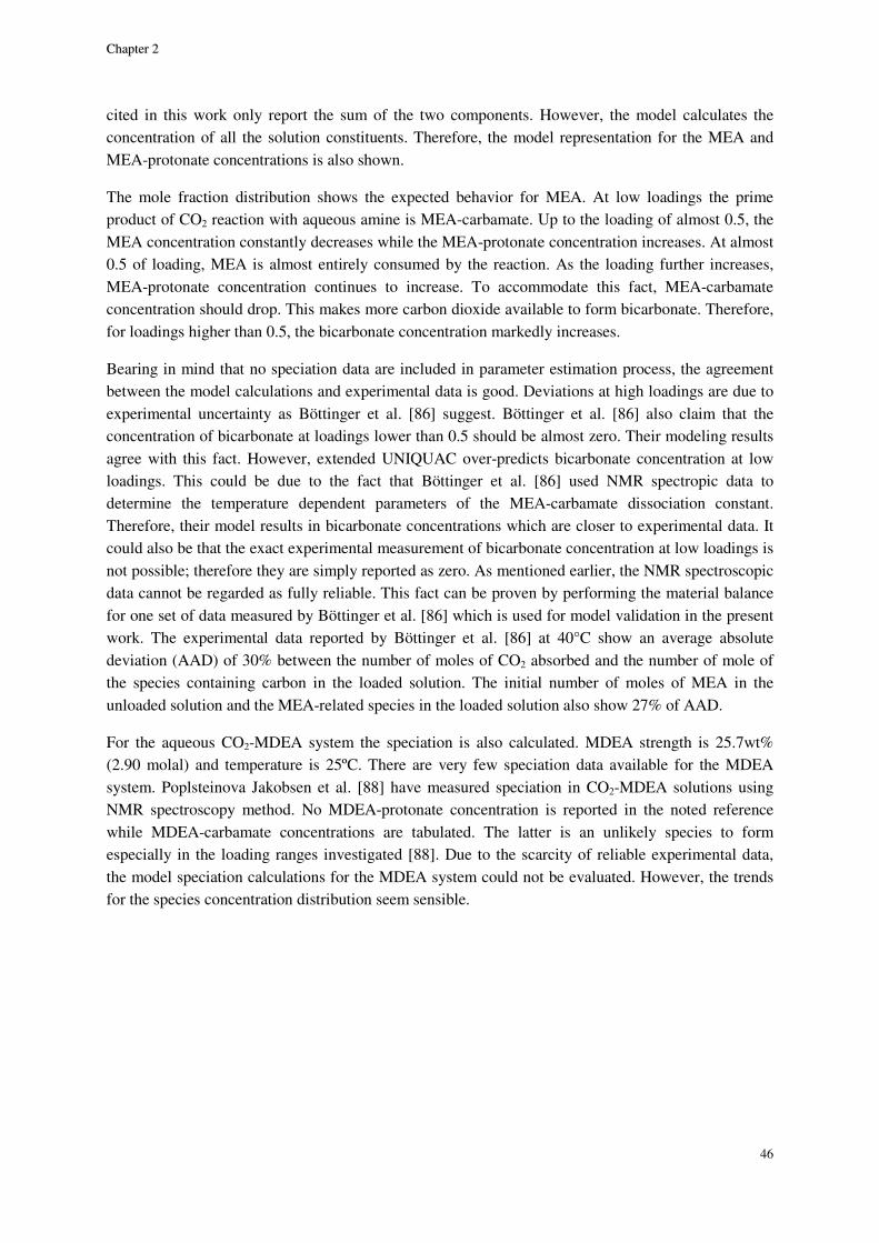
CChhaapptteerr 22
46
cited in this work only report the sum of the two components. However, the model calculates the concentration of all the solution constituents. Therefore, the model representation for the MEA and MEA-protonate concentrations is also shown.
The mole fraction distribution shows the expected behavior for MEA. At low loadings the prime product of CO2 reaction with aqueous amine is MEA-carbamate. Up to the loading of almost 0.5, the MEA concentration constantly decreases while the MEA-protonate concentration increases. At almost 0.5 of loading, MEA is almost entirely consumed by the reaction. As the loading further increases, MEA-protonate concentration continues to increase. To accommodate this fact, MEA-carbamate concentration should drop. This makes more carbon dioxide available to form bicarbonate. Therefore, for loadings higher than 0.5, the bicarbonate concentration markedly increases.
Bearing in mind that no speciation data are included in parameter estimation process, the agreement between the model calculations and experimental data is good. Deviations at high loadings are due to experimental uncertainty as Böttinger et al. [86] suggest. Böttinger et al. [86] also claim that the concentration of bicarbonate at loadings lower than 0.5 should be almost zero. Their modeling results agree with this fact. However, extended UNIQUAC over-predicts bicarbonate concentration at low loadings. This could be due to the fact that Böttinger et al. [86] used NMR spectropic data to determine the temperature dependent parameters of the MEA-carbamate dissociation constant. Therefore, their model results in bicarbonate concentrations which are closer to experimental data. It could also be that the exact experimental measurement of bicarbonate concentration at low loadings is not possible; therefore they are simply reported as zero. As mentioned earlier, the NMR spectroscopic data cannot be regarded as fully reliable. This fact can be proven by performing the material balance for one set of data measured by Böttinger et al. [86] which is used for model validation in the present work. The experimental data reported by Böttinger et al. [86] at 40°C show an average absolute deviation (AAD) of 30% between the number of moles of CO2 absorbed and the number of mole of the species containing carbon in the loaded solution. The initial number of moles of MEA in the unloaded solution and the MEA-related species in the loaded solution also show 27% of AAD.
For the aqueous CO2-MDEA system the speciation is also calculated. MDEA strength is 25.7wt% (2.90 molal) and temperature is 25ºC. There are very few speciation data available for the MDEA system. Poplsteinova Jakobsen et al. [88] have measured speciation in CO2-MDEA solutions using NMR spectroscopy method. No MDEA-protonate concentration is reported in the noted reference while MDEA-carbamate concentrations are tabulated. The latter is an unlikely species to form especially in the loading ranges investigated [88]. Due to the scarcity of reliable experimental data, the model speciation calculations for the MDEA system could not be evaluated. However, the trends for the species concentration distribution seem sensible.
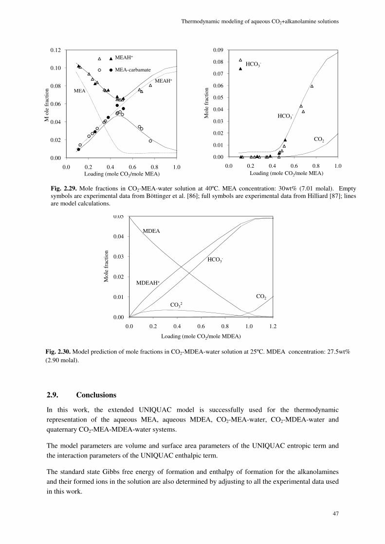
Thermodynamic modeling of aqueous CO2+alkanolamine solutions
47
2.9. Conclusions
In this work, the extended UNIQUAC model is successfully used for the thermodynamic representation of the aqueous MEA, aqueous MDEA, CO2-MEA-water, CO2-MDEA-water and quaternary CO2-MEA-MDEA-water systems.
The model parameters are volume and surface area parameters of the UNIQUAC entropic term and the interaction parameters of the UNIQUAC enthalpic term.
The standard state Gibbs free energy of formation and enthalpy of formation for the alkanolamines and their formed ions in the solution are also determined by adjusting to all the experimental data used in this work.
0.00
0.01
0.02
0.03
0.04
0.05
0.0 0.2 0.4 0.6 0.8 1.0 1.2
Mol
e fr
actio
n
Loading (mole CO2/mole MDEA)
MDEA
MDEAH+
HCO3-
CO32
CO2
0.00
0.02
0.04
0.06
0.08
0.10
0.12
0.0 0.2 0.4 0.6 0.8 1.0
M o
le f
ract
ion
Loading (mole CO2/mole MEA)
MEA
MEAH+
MEAH+
MEA-carbamate
0.00
0.01
0.02
0.03
0.04
0.05
0.06
0.07
0.08
0.09
0.0 0.2 0.4 0.6 0.8 1.0
Mol
e fr
actio
n
Loading (mole CO2/mole MEA)
HCO3-
CO2
HCO3-
Fig. 2.29. Mole fractions in CO2-MEA-water solution at 40ºC. MEA concentration: 30wt% (7.01 molal). Empty symbols are experimental data from Böttinger et al. [86]; full symbols are experimental data from Hilliard [87]; lines are model calculations.
Fig. 2.30. Model prediction of mole fractions in CO2-MDEA-water solution at 25ºC. MDEA concentration: 27.5wt% (2.90 molal).
CChhaapptteerr 22
48
There is a large body of experimental ternary VLE data available in the literature. The result of the analysis of the VLE data for the MDEA aqueous solutions showed that, most of the inconsistency between the data reported by different authors takes place in the low loading range.
Compared to other modeling approaches in the literature, a quite extensive range of pressure, temperature and CO2 concentration in the aqueous phase is addressed. Yet, the model’s performance is quite satisfactory for the calculation of VLE of MEA, MDEA and MEA+MDEA systems.
Freezing point depression for the aqueous alkanolamine systems is also calculated very precisely by the model.
The model correlates the excess enthalpy of MEA-water and MDEA-water systems reasonably well considering the scatter of experimental data. It is worthwhile to mention that the excess enthalpy data available in the literature are limited.
The calculated concentration distributions for both MEA and MDEA systems show the expected behavior. Considering that the model is not tuned to any speciation data and the uncertainty of experimental measurements, the model calculations are reasonable. This fact also proves the accuracy of the activity coefficients and also the standard state properties determined in the present work.
Overall, it has been shown that extended UNIQUAC can accurately represent physical and chemical equilibria (HE, VLE, SLE, speciation) over a wide range of conditions, thus being a valuable thermodynamic model for the design of the CO2 absorption plants.
List of symbols
A Debye-Hückel parameter (kg1/2 mol-1/2) A activity a, b, c parameters of equation 23 aq aqueous b Debye-Hückel parameter (kg1/2 mol-1/2) d density (kg m-3) F Faraday’s constant (C mol-1) G molar Gibbs energy (J mol-1) H enthalpy (J mol-1) I ionic strength based on molality M Molecular weight (kg mol-1) M molality (mol/kg H2O) NA Avogadro’s number n mole number P pressure (kPa) Q surface area R gas constant (J mol-1 K-1) R volume parameter S objective function T temperature (K) u, u
0, u
T UNIQUAC interaction parameters
x liquid phase mole fraction y vapor phase mole fraction z ionic charge
Thermodynamic modeling of aqueous CO2+alkanolamine solutions
49
Greek letters
∆ increment γ activity coefficient
ε0 vacuum permittivity (C- J-1 m-1) εr relative permittivity (dimensionless) µ chemical potential ν stochiometric coefficient φ fugacity coefficient
Sub/superscripts
∞ infinite dilution
0 standard state
* asymmetrical E excess
i index
j index
l liquid
v vapor w water x rational (mole fraction based) calc calculated exp experimental
References
[1] J.A. McLees, M. S. E. Thesis, the University of Texas at Austin, 2006. [2] E.J. Stewart, R.A. Lanning, Hydrocarbon Proc. 73 (1994) 67-81. [3] R.L. Kent, B. Eisenberg, Hydrocarbon Proc. 55 (1976) 87-90. [4] J. Gabrielsen, M.L. Michelsen, E.H. Stenby, G.M. Kontogeorgis, Ind. Eng. Chem. Res. 44 (2005) 3348-3354. [5] L. Chunxi, W. Fürst, Chem. Eng. Sci. 55 (2000) 2975-2988. [6] E. Solbraa, Ph.D. Thesis, Norwegian University of Science and Technology, 2002. [7] P.J.G. Huttenhuis, N.J. Agrawal, E. Solbraa, G.F. Versteeg, Fluid Phase Equilib. 264 (2008) 99-112. [8] W. Fürst, H. Renon, AIChE J. 39 (1993) 335-343. [9] G.M. Kontogeorgis, E.C. Voutsas, I.V. Yakoumis, D.P. Tassios, Ind. Eng. Chem. Res. 35 (1996) 4310-4318. [10] M.L. Posey, G.T. Rochelle, Ind. Eng. Chem. Res. 36 (1997) 3944-3953. [11] D.M. Austgen, G.T. Rochelle, X. Peng, C-C Chen, Ind. Eng. Chem. Res. 28 (1989) 1060-1073. [12] D.M. Austgen, G.T. Rochelle, C-C Chen, Ind. Eng. Chem. Res. 30 (1991) 543-555. [13] K. Thomsen, P. Rasmussen, Chem. Eng. Sci. 54 (1999) 1787-1802. [14] NIST Chemical Thermodynamics Database Version 1.1, U.S. Department of Commerce, National Institute of Standards and Technology, Gaithesburg, MD 20899, 1990. [15] J-H Kim, C. Dobrogowska, L.G. Hepler, Can. J. Chem. 65 (1986) 1726-1728. [16] M.K. Aroua, A. Benamor, M.Z. Haji-Sulaiman, J. Chem. Eng. Data 44 (1999) 887-891. [17] A. Perez-Salado Kamps, G. Maurer, J. Chem. Eng. Data 41 (1996) 1505-1513. [18] DIPPR (Design Institute for Physical Properties), Version 1.1.0, Predicted by Project Staff at the Pennsylvania State University using either published or internal methods. [19] K. Thomsen, Electrolyte Solutions: Thermodynamics, Crystallization, Separation Methods, Technical University of Denmark, 2006. [20] P. Debye, E. Hückel, Phys. Z. 24 (1923) 185. [21] K. S. Pitzer, Activity Coefficients in Electrolyte Solutions, CRC Press, Boca Raton, FL, 1991. [22] K. Thomsen, Pure Appl. Chem. 77 (3) (2005) 531-542. [23] C-C. Chen, H. I. Britt, J. F. Boston, L. B. Evans, AIChE J. 24 (1982) 588. [24] C-C. Chen, L.B. Evans, AIChE J. 32 (1986) 444-454. [25] K. Thomsen , P. Rasmussen , R. Gani, Chem. Eng. Sci. 51 (1996) 3675. [26] J. A. Myers, Sandler S. I., Wood R. H., Ind. Eng. Chem. Res. 41 (2002) 3282. [27] B. Sander, Aa. Fredenslund, P. Rasmussen, Chem. Eng. Sci. 41 (1986) 1171-1183. [28] H. Nicolaisen, P. Rasmussen , J.M. Sørensen, Chem. Eng. Sci. 48 (1993) 3149-3158. [29] D. S. Abrams, J. M. Prausnitz, AIChE J. 21 (1975) 116-128. [30] G. Maurer, J. M. Prausnitz, Fluid Phase Equilib. 2 (1978) 91-99. [31] Sir R. Fowler, E. A. Guggenheim, Statistical Thermodynamics, University Press, Cambridge, 1949. [32] Á. Pérez-Salado Kamps, Ind. Eng. Chem. Res., 44 (2005) 201. [33] K. Thomsen, Ph.D. Thesis, Department of Chemical Engineering, Technical University of Denmark, 1997.

CChhaapptteerr 22
50
[34] M. Iliuta, K. Thomsen and P. Rasmussen, Chem. Eng. Science, 55 (2000) 2673. [35] C-C. Chen and Y. Song, AIChE J. 50 (8) (2004) 1928. [36] J. Addicks, Ph.D Dissertation, Norwegian University of Technology, 2002. [37] E. E. Isaacs, F.D. Otto, A.E. Mather, J. Chem. Eng. Data 25 (1980) 118-120. [38] J. I. Lee, F.D. Otto, A.E. Mather, J. Appl. Chem. Biotechnol. 26 (1976) 541-549. [39] R.N. Maddox, A.H. Bhairi, J.R. Diers, P.A. Thomas, Gas Processors Association (GPA) Research Report RR-104 (1987). [40] A. Chakma, A. Meisen, Ind. Eng. Chem. Res. 26 (1987) 2461-66. [41] F-Y Jou, A.E. Mather, F.D. Otto, Ind. Eng. Chem. Process Des. Dev. 21 (1982) 539-44. [42] F-Y Jou, J.J. Carroll, A.E. Mather, F.D. Otto, Can. J. Chem. Eng. 71 (1993) 264-268. [43] B. Si Ali, M.K. Aroua, Int. J. Thermophys. 25 (2004) 1863-1870. [44] J. A. Barker, Austral. J. Chem., 6 (1953) 207-210. [45]H.C. Van Ness, F. Pedersen, P. Rasmussen, AICHE J. 24 (6) (1978) 1055-1063. [46] M-H Li, K-P Shen, J. Chem. Eng. Data 37 (1992) 288-290. [47] H.A. Al-Ghawas, D.P. Hagewiesche, G. Ruiz-Ibanez, O.C. Sandall, J. Chem. Eng. Data 34 (1989) 385-391. [48] E.B. Rinker, D.W. Oelschlager, A.T. Colussi, K.R. Henry, O.C. Sandall, J. Chem. Eng. Data 39 (1994) 392-395. [49] D.P. Hagewiesche, S.S. Ashour, H.A. Al-Ghawas, O.C. Sandall, Chem. Eng. Sci. 50 (1995) 1071-1079. [50] C.H. Hsu, M.H. Li, J. Chem. Eng. Data 42 (1997) 502-507. [51] H.T. Chang, M.L. Posey, G.T. Rochelle, Ind. Eng. Chem. Res. 32 (1993) 2324-2335. [52] Z-Y Cai, R-J Xie, Z-L Wu, J. Chem. Eng. Data 41 (1996) 1101-1103. [53] G. Kling, G. Maurer, J. Chem. Eng. Data 36 (1991) 390-394. [54] A. Nath, E. Bender, J. Chem. Eng. Data 28 (1983) 370-375. [55] K. Tochigi, K. Akimoto, K. Ochi, F. Liu, Y. Kawase, J. Chem. Eng. Data 44 (1999) 588-590. [56] H. Touhara, S. Okazaki, F. Okino, H. Tanaka, K. Ikari, K. Nakanishi, J. Chem. Thermodyn. 14 (1982) 145-156. [57] V. Dohnal, A.H. Roux, V. Hynek, J. Solution Chem. 23 (1994) 889-900. [58] M.L. Posey, Ph.D. Thesis, The University of Texas at Austin, 1996. [59] E. Voutsas, A. Vrachnos, K. Magoulas, Fluid Phase Equilib. 224 (2004). [60] Y. Maham, A.E. Mather, L.G. Hepler, J. Chem. Eng. Data 42 (1997) 988-992. [61] Y. Maham, A.E. Mather, C. Mathonat, J. Chem. Thermodyn. 32 (2000) 229-236 [62] G.T. Rochelle, S. Bishnoi, S. Chi, H. Dang, J. Santos, Final report for P.O. No. DE-AF26-99FT01029, US Department of Energy, Federal Energy Technology Center, Pittsburgh, 2001. [63] B. Rumpf, H. Nicolaisen, G. Maurer, Berichte der Bunsen-Gesellschaft 98 (1994) 1077-1081. [64] U. Göppert, G. Maurer, Fluid Phase Equilib. 41 (1988) 153-185. [65] N. Daneshvar, M.T. Zaafarani Moattar, M. Abedinzadegan Abdi, S. Aber, Sep. Purif. Technol. 37 (2004) 135-147. [66] F-Y Jou, A.E. Mather, F.D. Otto, Can. J. Chem. 73 (1995) 140-147. [67] J.D. Lawson, AW. Garst, J. Chem. Eng. Data 21 (1976) 20-30. [68] K-P Shen, M-H Li, J. Chem. Eng. Data 37 (1992) 96-100. [69] R. Sidi-Boumedine, S. Horstmann, K. Fischer, E. Provost, W. Fürst, J. Gmehling, Fluid Phase Equilib. 218 (2004) 85-94. [70] G. Kuranov, B. Rumpf, N.A. Smirnova, G. Maurer, Ind. Eng. Chem. Res. 35 (1996) 1959-1966. [71] S.W. Rho, K.P. Yoo, J.S. Lee, S.C. Nam, J.E. Son, B.M. Min, J. Chem. Eng. Data 42 (1997) 1161-1164. [72] C. Mathonat, V. Majer, A.E. Mather, J-P E. Grolier, Fluid Phase Equilib. 140 (1997) 171-182. [73] A. Perez-Salado Kamps, B. Rumpf, G. Maurer, AICHE J. 48 (2002) 168-177. [74] A. Perez-Salado Kamps, A. Balaban, M. Joedecke, G. Kuranov, N.A. Smirnova, G. Maurer, Ind. Eng. Chem. Res. 40 (2001) 696-706. [75] S. Ma'mun, R. Nilsen, H.F. Svendsen, J. Chem. Eng. Data 50 (2005) 630-634. [76] V. Ermatchkov, A. Perez-Salado, G. Maurer, Ind. Eng. Chem. Res. 45 (2006) 6081-6091. [77] H. Kierzkowska-Pawlak, Sep. Sci. Technol. 42 (2007) 2723-2737. [78] J-Y Park, S-J Yoon, H. Lee, Environ. Sci. Technol. 37 (2003) 1670-1675. [79] M.K. Aroua, R.M. Salleh, Chem. Eng. Technol. 27 (1) (2004) 65-70. [80] P.W.J. Derks, H.B.S. Dijkstra, J.A. Hogendoorn, G.F.Versteeg, AICHE J. 51 (8) (2005) 2311-2327. [81] S. Bishnoi, G.T. Rochelle G.T. AICHE J. 48(12) (2002) 2788-2799. [82] M. Kundu, S.S. Bandyopadhyay, Fluid Phase Equilib. 248 (2) (2006) 158-167. [83] D.M. VonNiederhausern, G.M. Wilson, N.F.J. Giles, J. Chem. Eng. Data 51 (2006) 1990-1995. [84] S. Xu, S. Qing, Z. Zhen, C. Zhang, J.J. Carroll, Fluid Phase Equilib. 67 (1991) 197-201. [85] O. F. Dawodu, A. Meisen, J. Chem. Eng. Data 39 (1994) 548-552. [86] W. Böttinger, M. Maiwald, H. Hasse, Fluid Phase Equilib. 263 (2008) 131-143. [87] M. Hilliard, Ph.D. Dissertation, University of Texas at Austin, 2008. [88] J. Poplsteinova Jakobsen, J. Krane, H. F. Svendsen, Ind. Eng. Chem. Res. 44 (2005) 9894-9903. [89] L. Faramarzi, G. M. Kontogeorgis, K. Thomsen, E. H. Stenby, Fluid Phase Equilib. 282 (2) (2009) 121-132.
33
MODELING THE MEA ABSORBER
The rate-based steady state model proposed by Gabrielsen et al. [Gabrielsen, Michelsen,
Kontogeorgis, Stenby, AICHE J. 52(10) (2006), 3443-3451] for the design of the CO2- 2-amino-2-
methyl-propanol (AMP) absorbers is adopted and improved for the design of the CO2-
monoethanolamine (MEA) absorber. The influence of the application of different mass transfer
correlations on the model’s performance is investigated. Analytical expressions for the calculation of
the enhancement factor for the second order as well as the pseudo-first order reaction regime are
integrated in the model and their impact on the model’s prediction is compared.
The model has been successfully applied to CO2 absorber packed columns and validated
against pilot plant data with good agreement [Faramarzi, Kontogeorgis, Michelsen, Thomsen,
Stenby, Ind. Eng. Chem. Res. 49 (8) (2010) 3751-3759].
Modeling the absorber
52
3.1. Introduction
Packed column absorbers employing aqueous alkanolamine solutions have long been used for purification of natural gas and separation of acidic gases from industrial gaseous streams. Despite the fact that the process has been studied for many years and there have been many modeling approaches adopted by researchers, the available models need to be enhanced and there is room for developing new consistent ones.
Apart from the unsound design methods, the scarcity of the reliable design and pilot plant data has been a major obstacle in modeling the chemical absorption processes such as CO2 capture in MEA solution.
One of the early works based on the rate-based approach for modeling a packed column absorber is that of Danckwerts and Alper [1]. De Leye and Froment [2] developed integrated design equations for chemical gas absorption considering the process as isothermal. Pandya [3] modeled the adiabatic rate-based CO2 absorption with amine and potash solutions. He described the liquid and gas phases as ideal and applied an explicit expression for the enhancement factor. Kucka et al. [4] established an elaborate rate-based model for absorption with MEA which involves solving a system of partial differential and algebraic equations. To solve the equations discretization was preformed both in the axial and film direction. The effect of reaction on the liquid-side mass transfer coefficient was accounted for rigorously but without application of enhancement factors. Alatiqi et al. [5] developed another rigorous rate-based model for absorption in a packed column using MEA. Their steady-stated model is based on a mixing cell approach and uses enhancement factors. Tobiesen et al. [6] presented another yet intricate model for CO2 absorption in MEA which is based on the penetration theory of mass transfer where the liquid-side is discretized using an adoptive gird. Several enhancement models are used for calculation of the mass transfer rate.
The rigorous models for the chemical absorption process generally provide a superior insight on mass transfer in the liquid boundary layer. However, in the absence of reliable methods and data required, rigorous modeling may not be advantageous. The user of such models may get involved in time consuming calculations where even a simple model could be adequate.
In the present work, the rate-based steady-state model presented by Gabrielsen et al. [7] is tailored to be applicable to the CO2-MEA systems. It is tried to keep the model as simple as possible and it is intended to show that the developed simple model can be an effective tool for simulation of the capture process.
3.2. The chemistry of the aqueous CO2-MEA system
The prime reactions taking place in the CO2-MEA system are:
MEA deprotonation:
3 2 3 3R NH H O H O R N→←+ ++ +
(3.1)
Carbamate reversion:
Chapter 3
53
(3.2)
R can represent alkyl group, alkanol group or hydrogen.
CO2 can also directly react with water to form rapidly dissociating carbonic acid; however, the reaction rate is insignificant except at high pH values.
In the loading region below 0.48, the equilibrium reaction of CO2 with aqueous MEA can be approximated by a single chemical reaction (Astarita [8]):
2 3 2 2 3 2R N CO H O R NH R NCOO→←+ −+ + + (3.3)
implying that all the absorbed CO2 reacts with the alkanolamine to form carbamate. The expression neglects the presence of bicarbonate (HCO3
+), hydroxide (OH-), and carbonate (CO32-) ions. In the
loading ranges of interest to CO2 capture from fossil fueled power plants using MEA, concentration of these ions will be very small. The area of interest is where the fast carbamate reaction dominates.
3.3. Absorption model
The mathematical model developed by Gabrielsen et al. [7] for the design of the CO2-AMP absorber packed columns is adopted and modified for the design of the CO2-MEA absorbers. This model is based on the material and energy balances around a differential element of a column and is founded on the work of Pandya [3].
The present absorber model is based on the two-film theory for mass transfer. The film model follows the simplest theory of mass transfer which leads to a set of steady state equations.
A collocation method is used to solve the system of differential equations by using a Fortran boundary value problem (BVP) solver developed by Shampine et al. [9]. When using this BVP solver, only the boundary values i.e. the conditions of the inlet gas and liquid need to be specified.
Moreover, for the variables for which the system is solved an initial guess for the profile of the values of the variables must be provided as well as an initial guess for the number and position of mesh points needed to solve the system. The BVP solver though shows little sensitivity to the chosen initial estimates.
The modifications to the Gabrielsen et al. [7] model are described in the following sections.
3.3.1. Enhancement factor
The absorption rate of acid gases in alkanolamine solutions is controlled by thermodynamics, which establishes the driving force for absorption, and reaction kinetics which has the capability to enhance the absorption rate far beyond what would be expected on the basis of physical absorption alone.
2 2 3 3R NCOO H O R N HCO→←− −+ +
Modeling the absorber
54
A frequent way of accounting for the effect of the chemical reaction on the liquid-side mass transfer coefficient is the application of the so-called enhancement factors. The enhancement factor E is the ratio of the amount of the gas absorbed in a reacting system to the amount which would be absorbed in case of no reaction taking place.
The analytical expression for the enhancement factor depends on the mass transfer theory applied as well as the kinetic definition of the reaction.
The expressions available for the enhancement factors for the mass transfer described by the film theory, as well as penetration and surface renewal theories are functions of the well-known Hatta number [10]. In the case of the film theory, the enhancement factor expressions is simpler compared to the former two theories.
For a reaction which is of the mth order with respect to the dissolved gas and of the order n in relation to the liquid-phase reactant, the Hatta number is:
( ) 12/ 1 ,m nm k C C Dm n ii j
HakL
−+= (3.4)
where km,n is the reaction rate constant and Di the diffusion coefficient of the gas compound in the aqueous phase. Ci and Cj indicate the concentrations of the gas component and the reactant in the aqueous phase [11] and kL is the liquid-side mass transfer coefficient of the solute gas.
What follows, briefly explains the influence of the mass transfer model and the considered reaction scheme on the equations for the enhancement factor.
3.3.1.1. Modelling of mass transfer in liquid boundary layer: Physical mass transfer The steady-state diffusion of compounds in the liquid phase due to the concentration gradient can be presented by the following equation:
0N
x
∂=
∂ (3.5)
where x is the distance from the gas-liquid interface into the liquid phase and N is the flux of the species of interest.
In the absence of any chemical reaction, the rate of absorption of CO2 in the mass transfer boundary layer depends on the Henry’s constant H, the liquid mass transfer coefficient, kL, and the gas liquid contact area, a:
[ ]2
2
2 bulk
3mol/cm( ) CO
L
CO
Pr k a CO
H
= −
(3.6)
To predict the mass transfer coefficient, a mass transfer model is needed. There are a number of theories developed to model mass transfer through a gas-liquid interface. The main mass transfer models are film theory, penetration theory, surface renewal theory and eddy diffusivity theory.
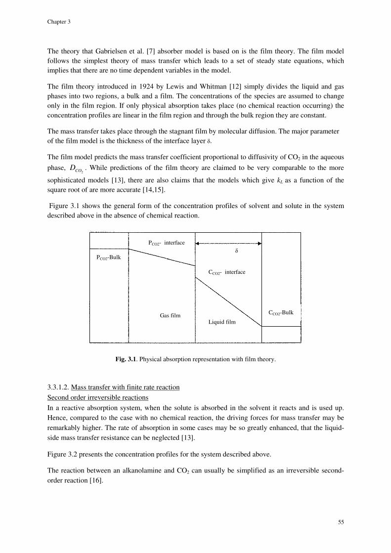
Chapter 3
55
The theory that Gabrielsen et al. [7] absorber model is based on is the film theory. The film model follows the simplest theory of mass transfer which leads to a set of steady state equations, which implies that there are no time dependent variables in the model.
The film theory introduced in 1924 by Lewis and Whitman [12] simply divides the liquid and gas phases into two regions, a bulk and a film. The concentrations of the species are assumed to change only in the film region. If only physical absorption takes place (no chemical reaction occurring) the concentration profiles are linear in the film region and through the bulk region they are constant.
The mass transfer takes place through the stagnant film by molecular diffusion. The major parameter of the film model is the thickness of the interface layer δ.
The film model predicts the mass transfer coefficient proportional to diffusivity of CO2 in the aqueous
phase, 2CO
D . While predictions of the film theory are claimed to be very comparable to the more
sophisticated models [13], there are also claims that the models which give kL as a function of the square root of are more accurate [14,15].
Figure 3.1 shows the general form of the concentration profiles of solvent and solute in the system described above in the absence of chemical reaction.
Fig. 3.1. Physical absorption representation with film theory.
3.3.1.2. Mass transfer with finite rate reaction Second order irreversible reactions
In a reactive absorption system, when the solute is absorbed in the solvent it reacts and is used up. Hence, compared to the case with no chemical reaction, the driving forces for mass transfer may be remarkably higher. The rate of absorption in some cases may be so greatly enhanced, that the liquid-side mass transfer resistance can be neglected [13].
Figure 3.2 presents the concentration profiles for the system described above.
The reaction between an alkanolamine and CO2 can usually be simplified as an irreversible second-order reaction [16].
PCO2-Bulk
Gas film
PCO2- interface
CCO2- interface
Liquid film
CCO2-Bulk
δ
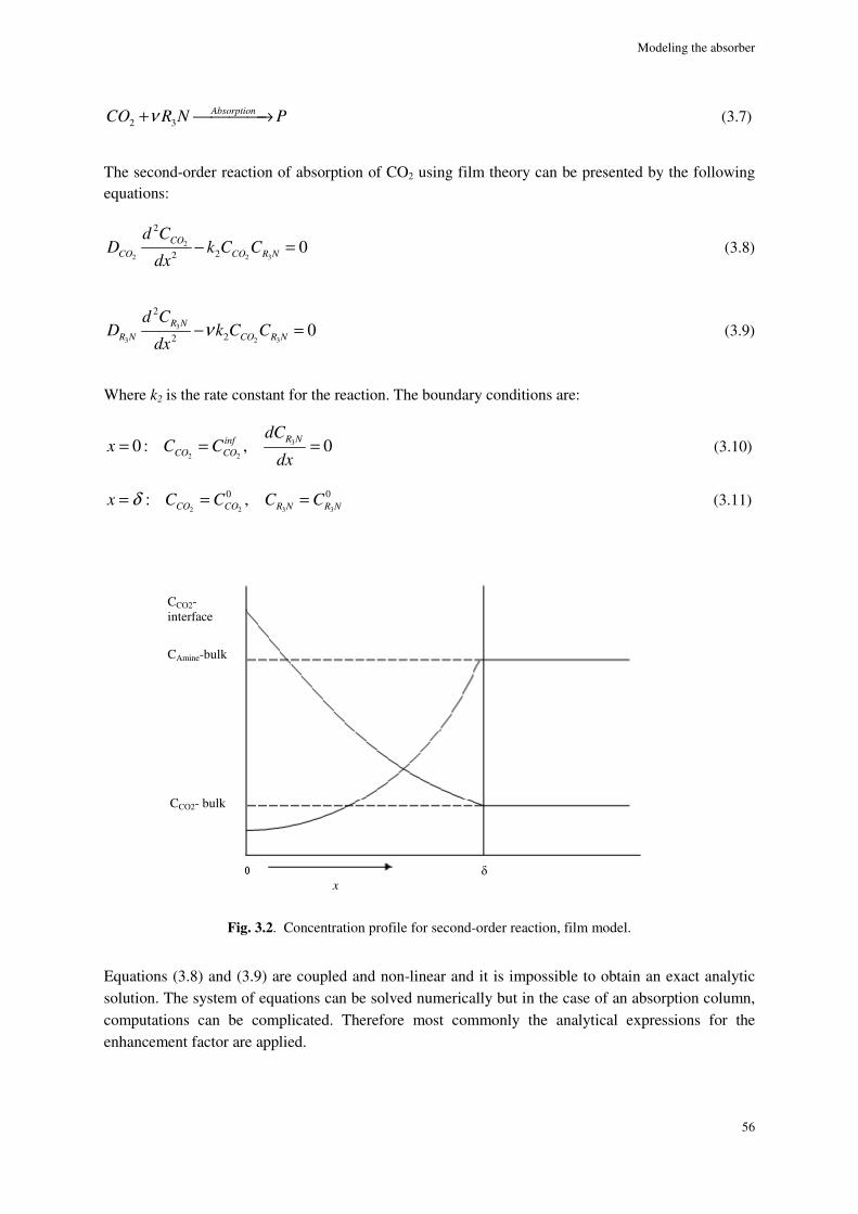
Modeling the absorber
56
2 3AbsorptionCO R N Pν+ → (3.7)
The second-order reaction of absorption of CO2 using film theory can be presented by the following equations:
2
2 2 3
2
220CO
CO CO R N
d CD k C C
dx− = (3.8)
3
3 2 3
2
220R N
R N CO R N
d CD k C C
dxν− = (3.9)
Where k2 is the rate constant for the reaction. The boundary conditions are:
3
2 20 : , 0R Ninf
CO CO
dCx C C
dx= = = (3.10)
2 2 3 3
0 0: ,CO CO R N R N
x C C C Cδ= = = (3.11)
Fig. 3.2. Concentration profile for second-order reaction, film model.
Equations (3.8) and (3.9) are coupled and non-linear and it is impossible to obtain an exact analytic solution. The system of equations can be solved numerically but in the case of an absorption column, computations can be complicated. Therefore most commonly the analytical expressions for the enhancement factor are applied.
CCO2- interface
CAmine-bulk
CCO2- bulk
x
δ
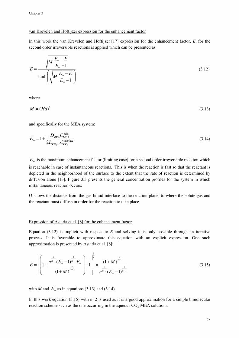
Chapter 3
57
van Krevelen and Hoftijzer expression for the enhancement factor
In this work the van Krevelen and Hoftijzer [17] expression for the enhancement factor, E, for the second order irreversible reactions is applied which can be presented as:
1
tanh1
E EM
EE
E EM
E
∞
∞
∞
∞
−
−=
−
−
(3.12)
where
2( )M Ha= (3.13)
and specifically for the MEA system:
2 2
bulkMEA MEA
interfaceCO , CO
12
L
D CE
D C∞ = + (3.14)
E∞ is the maximum enhancement factor (limiting case) for a second order irreversible reaction which
is reachable in case of instantaneous reactions. This is when the reaction is fast so that the reactant is depleted in the neighborhood of the surface to the extent that the rate of reaction is determined by diffusion alone [13]. Figure 3.3 presents the general concentration profiles for the system in which instantaneous reaction occurs.
Ω shows the distance from the gas-liquid interface to the reaction plane, to where the solute gas and the reactant must diffuse in order for the reaction to take place.
Expression of Astaria et al. [8] for the enhancement factor
Equation (3.12) is implicit with respect to E and solving it is only possible through an iterative process. It is favorable to approximate this equation with an explicit expression. One such approximation is presented by Astaria et al. [8]:
2 2
2 2
11
1 1
1 11 1
( 1) (1 )1 1
(1 ) ( 1)
n
n
n
n
n n
n n
n n
n E E ME
M n E
−
−
− −∞ ∞
− −∞
− + = + − ×
+ −
(3.15)
with M and E∞ as in equations (3.13) and (3.14).
In this work equation (3.15) with n=2 is used as it is a good approximation for a simple bimolecular reaction scheme such as the one occurring in the aqueous CO2-MEA solutions.
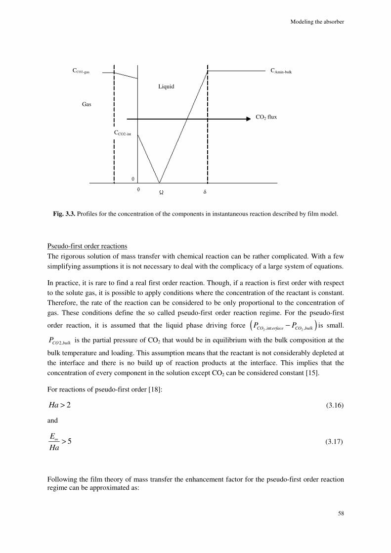
Modeling the absorber
58
Fig. 3.3. Profiles for the concentration of the components in instantaneous reaction described by film model.
Pseudo-first order reactions The rigorous solution of mass transfer with chemical reaction can be rather complicated. With a few simplifying assumptions it is not necessary to deal with the complicacy of a large system of equations.
In practice, it is rare to find a real first order reaction. Though, if a reaction is first order with respect to the solute gas, it is possible to apply conditions where the concentration of the reactant is constant. Therefore, the rate of the reaction can be considered to be only proportional to the concentration of gas. These conditions define the so called pseudo-first order reaction regime. For the pseudo-first
order reaction, it is assumed that the liquid phase driving force ( )2 2,int ,CO erface CO bulk
P P− is small.
2,CO bulkP is the partial pressure of CO2 that would be in equilibrium with the bulk composition at the
bulk temperature and loading. This assumption means that the reactant is not considerably depleted at the interface and there is no build up of reaction products at the interface. This implies that the concentration of every component in the solution except CO2 can be considered constant [15].
For reactions of pseudo-first order [18]:
2Ha > (3.16)
and
5E
Ha
∞ > (3.17)
Following the film theory of mass transfer the enhancement factor for the pseudo-first order reaction regime can be approximated as:
CCO2-gas
Gas
Liquid
CCO2-int
CAmin-bulk
CO2 flux
δ Ω
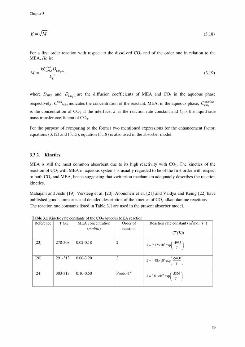
Chapter 3
59
E M= (3.18)
For a first order reaction with respect to the dissolved CO2 and of the order one in relation to the MEA, Ha is:
2 ,
2
bulk
MEA CO L
L
kC DM
k= (3.19)
where DMEA and 2 ,CO L
D are the diffusion coefficients of MEA and CO2 in the aqueous phase
respectively, CbulkMEA indicates the concentration of the reactant, MEA, in the aqueous phase,
2
interfaceCO
C
is the concentration of CO2 at the interface, k is the reaction rate constant and kL is the liquid-side mass transfer coefficient of CO2.
For the purpose of comparing to the former two mentioned expressions for the enhancement factor, equations (3.12) and (3.15), equation (3.18) is also used in the absorber model.
3.3.2. Kinetics
MEA is still the most common absorbent due to its high reactivity with CO2. The kinetics of the reaction of CO2 with MEA in aqueous systems is usually regarded to be of the first order with respect to both CO2 and MEA, hence suggesting that zwitterion mechanism adequately describes the reaction kinetics.
Mahajani and Joshi [19], Versteeg et al. [20], Aboudheir et al. [21] and Vaidya and Kenig [22] have published good summaries and detailed description of the kinetics of CO2-alkanolamine reactions. The reaction rate constants listed in Table 3.1 are used in the present absorber model. Table 3.1 Kinetic rate constants of the CO2/aqueous MEA reaction
Reference T (K) MEA concentration (mol/lit)
Order of reaction
Reaction rate constant (m3mol-1s-1)
(T (K))
[23] 278-308 0.02-0.18 2 7 -49559.77 10 expk
T
= ×
[20] 291-313 0.00-3.20 2 8 -54004.48 10 expk
T
= ×
[24] 303-313 0.10-0.50 Psudo-1st 8 -53763.01 10 expk
T
= ×
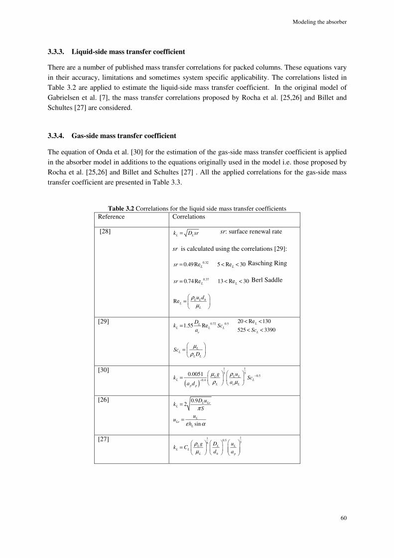
Modeling the absorber
60
3.3.3. Liquid-side mass transfer coefficient
There are a number of published mass transfer correlations for packed columns. These equations vary in their accuracy, limitations and sometimes system specific applicability. The correlations listed in Table 3.2 are applied to estimate the liquid-side mass transfer coefficient. In the original model of Gabrielsen et al. [7], the mass transfer correlations proposed by Rocha et al. [25,26] and Billet and Schultes [27] are considered.
3.3.4. Gas-side mass transfer coefficient
The equation of Onda et al. [30] for the estimation of the gas-side mass transfer coefficient is applied in the absorber model in additions to the equations originally used in the model i.e. those proposed by Rocha et al. [25,26] and Billet and Schultes [27] . All the applied correlations for the gas-side mass transfer coefficient are presented in Table 3.3.
Table 3.2 Correlations for the liquid side mass transfer coefficients
Reference Correlations
[28] L L
k D sr= sr: surface renewal rate
sr is calculated using the correlations [29]:
0.320.49Re 5 Re 30L L
sr = < < Rasching Ring
0.370.74Re 13 Re 30L L
sr = < < Berl Saddle
Re L L hL
L
u dρ
µ
=
[29] 0.72 0.5 20 Re 1301.55 Re
525 3390LL
L L L
Le
Dk Sc
Sca
< <=
< <
LL
L L
ScD
µ
ρ
=
[30]
( )
1133
0.50.4
0.0051 L L LL L
L e Lp p
g uk Sc
aa d
µ ρ
ρ µ−
−
=
[26] 0.92
sin
L LeL
LLe
L
D uk
S
uu
h
π
ε α
=
=
[27] 110.5
36L L L
L L
L h p
g D uk C
d a
ρ
µ
=
Chapter 3
61
3.3.5. Effective interfacial area of packing
The effective area of a packing under the loading point depends on its geometrical dimensions including the specific area, the liquid superficial velocity, the wettablity of the packing surface and also on the physical and chemical properties of the liquid phase [31].
Although there are many published works on the effective interfacial area of packing, there is still a great deal of controversy around the matter. Several definitions for the effective area exist amongst which the wetted surface area is of outmost importance. The wetted surface area can be taken as the reference area when considering mass transfer results. Moreover, under particular conditions, the wetted surface area can be closely linked to effective surface area because only the wetted area can be effective for mass transfer. Both the wetted surface area and the effective surface area are often applicable. The difference between the two is that the wetted surface area includes liquid surface areas in dead zones and the effective interfacial area includes surfaces of drops and jets [32].
One of the simplest equations available for the effective area is that of Onda et al. [30]. This correlation is developed for random packings based on the data for Rasching Ring, Berl Saddle, sphere and rod packings and ceramic Pall Ring. This correlation was obtained based on detailed investigation of hydrodynamics and liquid phase physical properties on the wetted surface area of random packings [32]. Onda et al. [30] have assumed that the effective mass transfer area is equal to the wetted surface area. This assumption may results in over-prediction of the effective interfacial area as the area of the dead zones are also being considered. This correlation also depends on the critical surface tension of the packing material and for materials of greater critical surface tension, even larger over-prediction may occur.
Cho [29] has proposed a simple correlation for the effective mass transfer area for Berl Saddle and Rasching Ring based on the data of absorption of chemical gas-liquid absorption.
Rocha et al. [25] have proposed a correlation for the structured packing which is the modification of an earlier equation by Shi and Mersmann [33] who assumed that the liquid flows in the form of uniformly distributed narrow streams inclined to the horizontal at an angle which partly wet the surface area of the packing. The dimensions of the streams were calculated by theoretical methods to obtain the wetted surface area and were measured by the experiments to validate predictive results. The authors [33] introduced a correction factor to consider the difference between the wetted and effective areas. This correction factor is a function of the packing diameter. Rocha et al. [26] added an alternative correction factor to the correlation of Shi and Mersmann [33]. Rocha et al. [26] also introduced a surface enhancement factor parameter which accounts for the enhancement of the packing surface.
Billet and Schultes [27] have proposed a set of equations for the calculation of specific surface area of packing. They have tested their equations for a variety of operating conditions and also different types and sizes of packing. These equations are claimed to well represent the experiments if the surface tension of the liquid along the column stays constant or increases. These systems are termed positive or neutral. In case of negative systems characterized by the decrease in surface tension along the column, the Marangoni effect must be taken into account because this effect will cause a reduction in the effective mass transfer area. In the case of absorption of CO2 in monoethanolamine, the system can be considered as positive, as the surface tension very slightly increases with loading but this change is said to be as small as it barely affects the performance of the column [34].
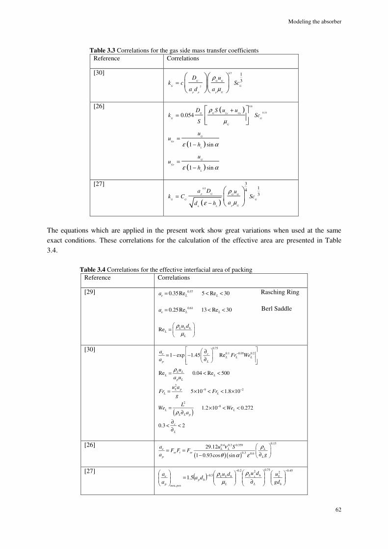
Modeling the absorber
62
Table 3.3 Correlations for the gas side mass transfer coefficients Reference Correlations
[30] 0.7
2
13G G G
G G
p p p G
D uk c Sc
a d a
ρ
µ=
[26] ( )
( )
( )
0.8
0.330.054
1 sin
1 sin
G G Le Ge
G G
G
G
Ge
L
G
Ge
L
D S u uk Sc
S
uu
h
uu
h
ρ
µ
ε α
ε α
+=
=−
=−
[27]
( )
0.5
3143p G G G
G G G
p Gh L
a D uk C Sc
ad h
ρ
µε=
−
The equations which are applied in the present work show great variations when used at the same exact conditions. These correlations for the calculation of the effective area are presented in Table 3.4.
Table 3.4 Correlations for the effective interfacial area of packing Reference Correlations
[29] 0.570.35Re 5 Re 30e L L
a = < < Rasching Ring
0.610.25Re 13 Re 30e L L
a = < < Berl Saddle
Re L L h
L
L
u dρ
µ
=
[30]
( )
0.75
0.1 0.05 0.2
29 2
28
1 exp 1.45 Re
Re 0.04 Re 500
5 10 1.8 10
1.2 10 0.272
0.3 2
e cL L L
p L
L LL L
p L
L p
L L
L L
L L p
c
L
aFr We
a
u
a u
u aFr Fr
g
LWe We
a
ρ
ρ
−
− −
−
∂ = − −
∂
= < <
= × < < ×
= × < <∂
∂< <
∂
[26]
( ) ( )
0.150.4 0.2 0.359
0.3 0.6
29.12
1 0.93cos sine L L L
se t se
p L
a u SF F F
a g
ν ρ
θ α ε
= =
∂−
[27] ( )
45.0275.022.0
5.0
,
5.1−−
−
∂
=
h
L
L
hL
L
hLLhp
posneup
e
gd
udududa
a
aL
ρ
µ
ρ
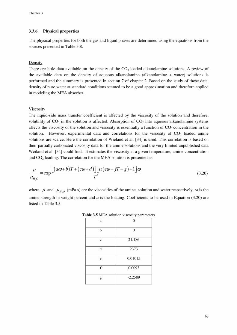
Chapter 3
63
3.3.6. Physical properties
The physical properties for both the gas and liquid phases are determined using the equations from the sources presented in Table 3.8.
Density There are little data available on the density of the CO2 loaded alkanolamine solutions. A review of the available data on the density of aqueous alkanolamine (alkanolamine + water) solutions is performed and the summary is presented in section 7 of chapter 2. Based on the study of those data, density of pure water at standard conditions seemed to be a good approximation and therefore applied in modeling the MEA absorber.
Viscosity The liquid-side mass transfer coefficient is affected by the viscosity of the solution and therefore, solubility of CO2 in the solution is affected. Absorption of CO2 into aqueous alkanolamine systems affects the viscosity of the solution and viscosity is essentially a function of CO2 concentration in the solution. However, experimental data and correlations for the viscosity of CO2 loaded amine solutions are scarce. Here the correlation of Wieland et al. [34] is used. This correlation is based on their partially carbonated viscosity data for the amine solutions and the very limited unpublished data Weiland et al. [34] could find. It estimates the viscosity at a given temperature, amine concentration and CO2 loading. The correlation for the MEA solution is presented as:
( ) ( ) ( )
2
2
1exp
H O
a b T c d e fT g
T
ω ω α ω ωµ
µ
+ + + + + + = (3.20)
where µ and 2H O
µ (mPa.s) are the viscosities of the amine solution and water respectively. is the
amine strength in weight percent and α is the loading. Coefficients to be used in Equation (3.20) are listed in Table 3.5.
Table 3.5 MEA solution viscosity parameters
a 0
b 0
c 21.186
d 2373
e 0.01015
f 0.0093
g -2.2589
Modeling the absorber
64
Weiland et al. [34] claim that the above correlation represents the viscosity data within the standard deviation of 0.0732. MEA concentration up to 40wt% was included in fitting the parameters of Equation (3.20) as well as loadings up to 0.6. The correlation is valid up to 398K.
Fig. 3.4. The viscosity of MEA aqueous solutions as a function of MEA strength and temperature.
Figure 3.4 presents the viscosities of the unloaded aqueous MEA solutions at various amine strengths calculated using the correlation of Weiland et al. [34].
Solubility For the rational design of gas absorption units physical solubility of acid gas is needed. This property which is measured as Henry’s law constant is required to model the rate of absorption.
For the moderately soluble gases with relatively little interaction between the gas and liquid molecules, Henry’s law is often applicable with the following expression:
i i
t
Hey x
P= (3.21)
where iy is the mole fraction of component i in the gas phase, tP is the total pressure, He is the
Henry’s constant and xi is the mole fraction of component i in the liquid phase. He is a function of temperature and is almost independent of pressure and for the electrolyte solutions where ionic species are present in the solution; it is also a function of the ionic strength of the solution. When carbon dioxide is absorbed in the alkanolamine solution, it reacts with amine and ions such as amine carbamate, bicarbonate and protonated amines are formed. By formation of theses ions and the increase in the ionic strength of the solution, the gas solubility is reduced. This phenomenon is known as the salting out effect. The relationship between the Henry’s law constant of such a solution and the ionic strength of the solution is given by van Krevelen correlation [35]:
*log
HehI
He
=
(3.22)
0.0000
0.0005
0.0010
0.0015
0.0020
0.0025
0.0030
0.0035
0 10 20 30 40
Vis
cosi
ty (
Pa.
s)
WT% MEA
49°C
110°C100°C82°C
65°C
32°C
Chapter 3
65
where He and He* are the Henry’s constants of the electrolyte solution and the pure molecular solvent
respectively, I is the ionic strength of the solution and h is sum of three constants which are dependent on the system
gh h h h+ −= + + (3.23)
where h+, h- and hg are the van Krevelen coefficients for the cation, anion and the dissolved gas, respectively [36].
As the absorption of CO2 in alkanolamine solutions is always along with chemical reaction, its physical solubility in amine solutions cannot be measured directly. One way of determining the physical solubility of carbon dioxide in amine solutions is therefore, the use of another gas which is similar to CO2 in shape, size, electronic configuration and Leonard-Jones potentials. The solubility of this gas is measured experimentally and the measured values are then used to calculate the solubility of CO2 by using proportionality constants. This Nitrous Oxide analogy is expressed as [34]:
, ,2 2
, ,2 2
CO Solution CO water
N O Solution N O water
He HeK
He He= = (3.24)
where K is the proportionality constant. Wieland [34] has set K equal to 0.73. It seems as if the figure 0.73 refers to the standard temperature of 25°C as this constant should change with the temperature of the solution.
The solubility of CO2 in water is well established and there are numerous data available in the literature. Also some authors have correlated CO2 solubility in water. Danckwerts and Sharma [37] have presented the following correlation
2
1140log 5.30
COHe
T− = −
(3.25)
where He° is the Henry’s constant of carbon dioxide in pure water.
Experimental data on physical solubility of N2O in some of the alkanolamine solutions are available in the open literature. In the present work the physical solubility data for the absorption of CO2 in different aqueous alkanolamine solutions are collected and analyzed. A summary of the open literature data surveyed follows. However it should be mentioned that only the data for the MEA system were eventually required for modeling the absorber column.
Haimour and Sandall [38] performed a set of experiments on the basis of the hypothesis of the N2O analogy for MDEA. The result of their experiments includes the data on solubility of N2O in MDEA solutions with strength of 0-40 wt% at temperatures of 15-35°C.
Al-Ghawas et al. [39] have published the experimental results of N2O analogy for the MDEA solutions of 0-50 wt% at 15-50°C. Browning and Weiland [36] have presented the data on the solubility of N2O in partially neutralized MEA, DEA and MDEA solutions. These data are all obtained at 25°C and the reason for partially neutralizing the solution with sulfuric acid has been to determine the van Krevelen coefficients for protonated amines in order to consider the effect of the
Modeling the absorber
66
protonated amine on the physical solubility of CO2 in the solution. Also for determination of the van Krevelen coefficients for carbamate, bicarbonate and carbonate ions, MEA, DEA and MDEA solutions with different strengths were partially loaded with CO2 and then the solubility data as well as the values determined for anionic coefficients at 25°C were reported.
In the last noted work the solubility data for N2O in partially CO2 loaded MDEA blends with MEA and DEA are also reported. Li and Lee [40] have measured the solubility of N2O in DEA+MDEA and DEA+AMP solutions at 30, 35 and 40°C. The total concentration of amine blend in the solution was set to 30wt%. Following the Nitrous oxide analogy and using Versteeg and van Swaaij [41] correlations for solubility of CO2 and N2O in water, they have also reported the solubility of CO2 in different amine solutions. Weiland [34] ran a set of experimental tests to determine the solubility of N2O in alkanolamine solutions at 25°C. The Henry’s constants of N2O in partially neutralized and also partially carbonated MEA solutions with the concentration of 10, 20 and 30 wt%, DEA solutions of 10, 20 ,30, 40 wt% and MDEA solutions of 10, 20 and 30wt% have been reported. It should be noted that the experiments were carried out at 25°C. Also the van Krevelen coefficients of MEAH+, DEAH+ and MDEAH+ cations and MEACOO-, DEACOO-, and HCO3
- anions are reported by Weiland [34] which are almost twice as the corresponding coefficients for NH4
+ and CO3-2 which are sometimes
used as estimate coefficients for protonated MEA and MEA carbamate. Tsai et al. [42] have measured the solubility of Nitrous oxide in alkanolamine aqueous solutions at 30, 35 and 40°C. The amine systems studied were MEA, DEA, di-isopropanolamine (DIPA), Tri-ethanolamine (TEA) and AMP. The concentration of MEA solution was in the range of 1-6 kmol.m-3 and for other amine systems it was 0.5-3 kmol.m-3. Mandal et al. [43] have determined the physical solubility of N2O in DEA, AMP, MDEA, MDEA+DEA, AMP+DEA solutions at temperatures of 20, 25, 30, 35 and 40°C. For single amine solutions the concentration of amine had been 2, 2.5 and 3 kmol.m-3 and for mixed amine solutions the total concentration of amine had been set to 30 wt%. Mandal et al. [44] have reported the Henry’s constants of CO2 in MEA, DEA and MDEA solutions of 2, 2.5 and 3 kmol.m-3 and for the amine mixtures of MDEA+MEA and AMP+MEA with the total strength of 30wt% at 20, 25, 30, 35 and 40°C. Table 3.6 presents a summary of the references of N2O solubility in alkanolamine solutions
reviewed.
Table 3.6 Literature review of CO2 Henry’s law constant of amine solutions Author Amine Concentration (wt%) Temperature (°C) Notes
[38] MDEA 0-40 15 - 35
[39] MDEA 0-50 15 -50
[36] MEA 10, 20, 30
25
The solubility data are both obtained for the partially neutralized and partially loaded solutions
DEA 10, 20, 30, 40
MDEA 20, 30, 40, 50
MEA + MDEA 10 + 40
MEA + MDEA 20 + 30
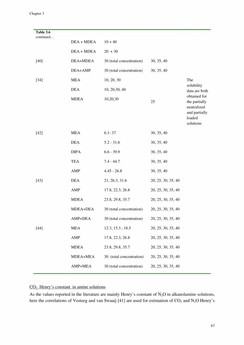
Chapter 3
67
Table 3.6 continued…
DEA + MDEA
DEA + MDEA
10 + 40
20 + 30
[40] DEA+MDEA 30 (total concentration) 30, 35, 40
DEA+AMP 30 (total concentration) 30, 35, 40
[34] MEA 10, 20, 30
25
The solubility data are both obtained for the partially neutralized and partially loaded solutions
DEA 10, 20,30, 40
MDEA 10,20,30
[42] MEA
DEA
6.1- 37
5.2 - 31.6
30, 35, 40
30, 35, 40
DIPA 6.6 - 39.9 30, 35, 40
TEA 7.4 - 44.7 30, 35, 40
AMP 4.45 - 26.8 30, 35, 40
[43] DEA 21, 26.3, 31.6 20, 25, 30, 35, 40
AMP 17.8, 22.3, 26.8 20, 25, 30, 35, 40
MDEA 23.8, 29.8, 35.7 20, 25, 30, 35, 40
MDEA+DEA 30 (total concentration) 20, 25, 30, 35, 40
AMP+DEA 30 (total concentration) 20, 25, 30, 35, 40
[44] MEA 12.3, 15.3 , 18.5 20, 25, 30, 35, 40
AMP 17.8, 22.3, 26.8 20, 25, 30, 35, 40
MDEA 23.8, 29.8, 35.7 20, 25, 30, 35, 40
MDEA+MEA 30 (total concentration) 20, 25, 30, 35, 40
AMP+MEA 30 (total concentration) 20, 25, 30, 35, 40
CO2 Henry’s constant in amine solutions
As the values reported in the literature are mainly Henry’s constant of N2O in alkanolamine solutions, here the correlations of Vesteeg and van Swaaij [41] are used for estimation of CO2 and N2O Henry’s
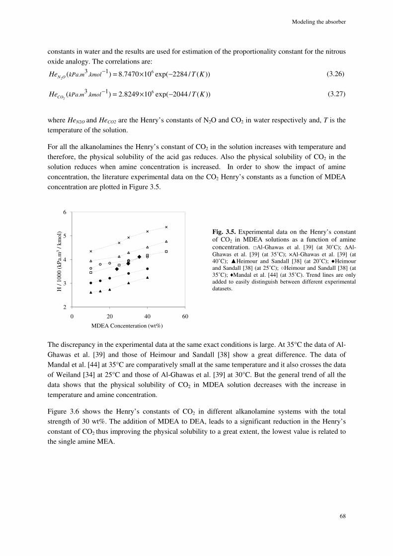
Modeling the absorber
68
constants in water and the results are used for estimation of the proportionality constant for the nitrous oxide analogy. The correlations are:
2
63 1. .( ) 8.7470 10 exp( 2284 / ( ))N O
kPa m kmolHe T K− = × − (3.26)
2
63 1. .( ) 2.8249 10 exp( 2044 / ( ))CO
kPa m kmolHe T K− = × − (3.27)
where HeN2O and HeCO2 are the Henry’s constants of N2O and CO2 in water respectively and, T is the temperature of the solution.
For all the alkanolamines the Henry’s constant of CO2 in the solution increases with temperature and therefore, the physical solubility of the acid gas reduces. Also the physical solubility of CO2 in the solution reduces when amine concentration is increased. In order to show the impact of amine concentration, the literature experimental data on the CO2 Henry’s constants as a function of MDEA concentration are plotted in Figure 3.5.
The discrepancy in the experimental data at the same exact conditions is large. At 35°C the data of Al-Ghawas et al. [39] and those of Heimour and Sandall [38] show a great difference. The data of Mandal et al. [44] at 35°C are comparatively small at the same temperature and it also crosses the data of Weiland [34] at 25°C and those of Al-Ghawas et al. [39] at 30°C. But the general trend of all the data shows that the physical solubility of CO2 in MDEA solution decreases with the increase in temperature and amine concentration.
Figure 3.6 shows the Henry’s constants of CO2 in different alkanolamine systems with the total strength of 30 wt%. The addition of MDEA to DEA, leads to a significant reduction in the Henry’s constant of CO2 thus improving the physical solubility to a great extent, the lowest value is related to the single amine MEA.
2
3
4
5
6
0 20 40 60
H /
1000
(kP
a.m
3/ k
mol
)
MDEA Concenteration (wt%)
Fig. 3.5. Experimental data on the Henry’s constant of CO2 in MDEA solutions as a function of amine concentration. Al-Ghawas et al. [39] (at 30˚C); Al-Ghawas et al. [39] (at 35˚C); ×Al-Ghawas et al. [39] (at 40˚C); Heimour and Sandall [38] (at 20˚C); Heimour and Sandall [38] (at 25˚C); Heimour and Sandall [38] (at 35˚C); ♦Mandal et al. [44] (at 35˚C). Trend lines are only added to easily distinguish between different experimental datasets.
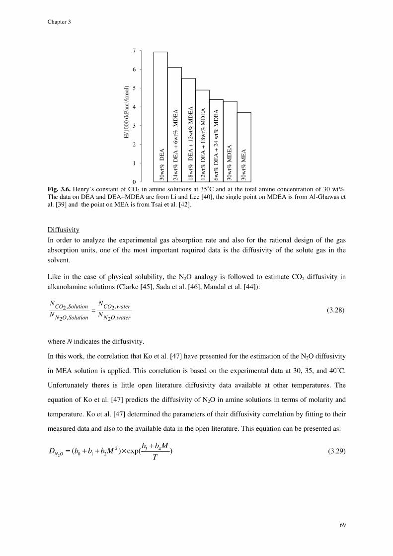
Chapter 3
Fig. 3.6. Henry’s constant of CO2 in amine solutions at 35The data on DEA and DEA+MDEA are from Li and Lee [40], al. [39] and the point on MEA is from Tsai et al. [42].
Diffusivity
In order to analyze the experimental gas absorption rate and also for the rational design of the gas absorption units, one of the most important required data is the diffusivity of the solute gas in the solvent.
Like in the case of physical solubility, thalkanolamine solutions (Clarke [45], Sada et al. [46], Mandal et al. [44]):
, ,2 2
, ,2 2
CO Solution CO water
N O Solution N O water
N N
N N=
where N indicates the diffusivity.
In this work, the correlation that Ko et al. [47
in MEA solution is applied. This correlation is based on the experimental data at 30, 35, and 40
Unfortunately theres is little open literature diffu
equation of Ko et al. [47] predicts the diffusivity of N
temperature. Ko et al. [47] determined the
measured data and also to the available data in the open literature. This equation can be presented as:
2
20 1 2( ) exp( )
N O
b b MD b b b M= + + ×
0
1
2
3
4
5
6
7
H/1
000
(kP
am3 /
kmol
)
in amine solutions at 35˚C and at the total amine concentration of 30 wt%.
d DEA+MDEA are from Li and Lee [40], the single point on MDEA is from AlMEA is from Tsai et al. [42].
In order to analyze the experimental gas absorption rate and also for the rational design of the gas absorption units, one of the most important required data is the diffusivity of the solute gas in the
Like in the case of physical solubility, the N2O analogy is followed to estimate COalkanolamine solutions (Clarke [45], Sada et al. [46], Mandal et al. [44]):
indicates the diffusivity.
orrelation that Ko et al. [47] have presented for the estimation of the N
in MEA solution is applied. This correlation is based on the experimental data at 30, 35, and 40
Unfortunately theres is little open literature diffusivity data available at other temperature
] predicts the diffusivity of N2O in amine solutions in terms of molarity and
Ko et al. [47] determined the parameters of their diffusivity correlation by fittin
the available data in the open literature. This equation can be presented as:
3 4( ) exp( )b b M
T
+
30w
t% D
EA
18w
t% D
EA
+ 12
wt%
MD
EA
24w
t%D
EA
+ 6
wt%
MD
EA
12w
t% D
EA
+ 1
8wt%
MD
EA
6wt%
DE
A +
24
wt%
MD
EA
30w
t% M
DE
A
30w
t% M
EA
69
concentration of 30 wt%. A is from Al-Ghawas et
In order to analyze the experimental gas absorption rate and also for the rational design of the gas absorption units, one of the most important required data is the diffusivity of the solute gas in the
O analogy is followed to estimate CO2 diffusivity in
(3.28)
] have presented for the estimation of the N2O diffusivity
in MEA solution is applied. This correlation is based on the experimental data at 30, 35, and 40˚C.
sivity data available at other temperatures. The
O in amine solutions in terms of molarity and
correlation by fitting to their
the available data in the open literature. This equation can be presented as:
(3.29)
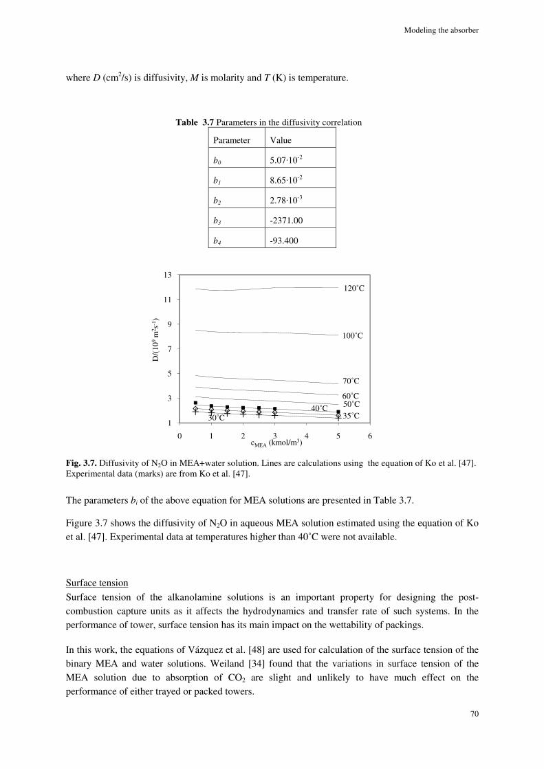
Modeling the absorber
70
where D (cm2/s) is diffusivity, M is molarity and T (K) is temperature.
Table 3.7 Parameters in the diffusivity correlation
Parameter Value
b0 5.07·10-2
b1 8.65·10-2
b2 2.78·10-3
b3 -2371.00
b4 -93.400
Fig. 3.7. Diffusivity of N2O in MEA+water solution. Lines are calculations using the equation of Ko et al. [47]. Experimental data (marks) are from Ko et al. [47].
The parameters bi of the above equation for MEA solutions are presented in Table 3.7.
Figure 3.7 shows the diffusivity of N2O in aqueous MEA solution estimated using the equation of Ko et al. [47]. Experimental data at temperatures higher than 40˚C were not available.
Surface tension Surface tension of the alkanolamine solutions is an important property for designing the post-combustion capture units as it affects the hydrodynamics and transfer rate of such systems. In the performance of tower, surface tension has its main impact on the wettability of packings.
In this work, the equations of Vázquez et al. [48] are used for calculation of the surface tension of the binary MEA and water solutions. Weiland [34] found that the variations in surface tension of the MEA solution due to absorption of CO2 are slight and unlikely to have much effect on the performance of either trayed or packed towers.
1
3
5
7
9
11
13
0 1 2 3 4 5 6
D/(
109
m2 s
-1)
cMEA (kmol/m3)
35˚C40˚C 50˚C
60˚C
100˚C
70˚C
30˚C
120˚C
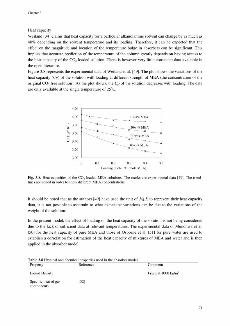
Chapter 3
Heat capacity Weiland [34] claims that heat capacity for a particular alkanolamine solvent can change by as much as 40% depending on the solvent effect on the magnitude and location of the temperature bulge in absorbers can be significant. This implies that accurate prediction of the temperature of the column greatly depends on havthe heat capacity of the CO2 loaded solution. There is however very little consistent data available in the open literature. Figure 3.8 represents the experimental data of Weiland et al. [heat capacity (Cp) of the solution with loading at different strength of MEA (the original CO2 free solution). As the plot shows, the are only available at the single temperature of 25
Fig. 3.8. Heat capacities of the COlines are added in order to show different MEA concentrations.
It should be noted that as the authors [49] have used the unit of data, it is not possible to ascertain to what extent the variations can be due to the variations of the weight of the solution.
In the present model, the effect of loading on the heat capacity of the solution is not being due to the lack of sufficient data at relevant temperatures. The experimental data of [50] for the heat capacity of pure MEA and those of Osborne et al. [51] for pure water are used to establish a correlation for estimation of theapplied in the absorber model. Table 3.8 Physical and chemical properties used in the absorber model.
Property Reference
Liquid Density
Specific heat of gas components
[52]
3.00
3.20
3.40
3.60
3.80
4.00
4.20
0
Cp
(J g
-1K
-1)
Weiland [34] claims that heat capacity for a particular alkanolamine solvent can change by as much as 40% depending on the solvent temperature and its loading. Therefore, it can be expected that the effect on the magnitude and location of the temperature bulge in absorbers can be significant. This implies that accurate prediction of the temperature of the column greatly depends on hav
loaded solution. There is however very little consistent data available in
represents the experimental data of Weiland et al. [49]. The plot shows the variations of theof the solution with loading at different strength of MEA (the
free solution). As the plot shows, the Cp of the solution decreases with loading. The data are only available at the single temperature of 25˚C.
Heat capacities of the CO2 loaded MEA solutions. The marks are experimental data [lines are added in order to show different MEA concentrations.
It should be noted that as the authors [49] have used the unit of J/g.K to represent their heat capacity data, it is not possible to ascertain to what extent the variations can be due to the variations of the
In the present model, the effect of loading on the heat capacity of the solution is not being due to the lack of sufficient data at relevant temperatures. The experimental data of
for the heat capacity of pure MEA and those of Osborne et al. [51] for pure water are used to establish a correlation for estimation of the heat capacity of mixtures of MEA and water and
Physical and chemical properties used in the absorber model. Reference Comment
Fixed at 1000 kg/m
[52]
0.1 0.2 0.3 0.4 0.5Loading (mole CO2/mole MEA)
20wt% MEA
30wt% MEA
40wt% MEA
10wt% MEA
71
Weiland [34] claims that heat capacity for a particular alkanolamine solvent can change by as much as temperature and its loading. Therefore, it can be expected that the
effect on the magnitude and location of the temperature bulge in absorbers can be significant. This implies that accurate prediction of the temperature of the column greatly depends on having access to
loaded solution. There is however very little consistent data available in
]. The plot shows the variations of the of the solution with loading at different strength of MEA (the concentration of the
of the solution decreases with loading. The data
loaded MEA solutions. The marks are experimental data [49]. The trend-
to represent their heat capacity data, it is not possible to ascertain to what extent the variations can be due to the variations of the
In the present model, the effect of loading on the heat capacity of the solution is not being considered due to the lack of sufficient data at relevant temperatures. The experimental data of Mundhwa et al.
for the heat capacity of pure MEA and those of Osborne et al. [51] for pure water are used to heat capacity of mixtures of MEA and water and is then
Fixed at 1000 kg/m3
Modeling the absorber
72
Table 3.8 continued...
Specific heat of liquid solution
[51] for water
[50] for pure MEA
Linear mixing of the heat capacities of water and pure MEA
Diffusivity of CO2 in the liquid solution
[47] Based on the N2O analogy
Viscosity of the gas [52] Method of Wilke
Thermal conductivity of the gas
[52] Eucken for pure compounds, Mason and Saxena for mixture
Diffusivity of CO2 and water in the gas phase
[52] Fuller equation
Surface tension of the liquid solution
[48]
Viscosity of the liquid solution
[53] for water and [34] for loaded solution
Henry’s Law Constant of CO2 in the liquid solution
[54]
[36]
Based on the N2O analogy and using an expression to account for the salting out effect with increased CO2 loading
Diffusivity of MEA in the liquid solution
[55]
3.3.7. Thermodynamics
The simple thermodynamic model developed by Gabrielsen et al. [56] is applied for the calculation of the equilibrium partial pressure of CO2 over the aqueous MEA solution and also of the speciation in the solution. In this work, equation 3 is the assumed equilibrium reaction between CO2 and MEA.
The heat of absorption of CO2 in the MEA solution is also calculated using an equation proposed by Gabrielsen et al. [56].To determine the equilibrium partial pressure of water over the solution an
Antoine equation is applied. The heat of vaporization of water ( 2H OH∆ ) is derived from the Antoine
equation using the Gibbs-Helmholtz equation.
A very detailed description of the thermodynamic model applied in the absorber model [56] is presented by Gabrielsen [16] therefore further explanation is avoided here.
3.4. Results and discussion
3.4.1. Pilot plant data used for simulation
The pilot plant data from Tontiwachwuthikul [57] are used in this work for comparison with the model predictions. The column used by Tontiwachwuthikul [57] is packed with 13mm Berl Saddle and the packed height of the bed is 6.55m. These data are particularly interesting due to the fact that
Chapter 3
73
apart from the conditions at both ends of the absorber, the profiles for the gas phase mole fraction of CO2, loading and temperature are also reported.
Some of the pilot plant data of Dugas [58] are also simulated. In the experiments [58] a column with the packed height of 6.10m is used where the type of packing is IMTP 40. But for the latter data [58], the actual agreement with the model predictions was not very satisfactory unless the absorber model was tuned to the pilot data. This could be well due to the inconsistency of the noted data which is also mentioned by Kvamsdal and Rochelle [59].
The specifications for the two columns are presented in Table 3.9. The required packing data for the 13mm ceramic Berl Saddle are obtained from Billet and Schultes [27]. Onda et al. [30] correlations also need the critical surface tension of the packing material which is obtained from McCabe et al. [60]. Packing specifications are presented in Table 3.10.
Table 3.9. Input pilot plant data applied for simulation
Reference Inlet gas flow(mol/s)
Inlet liquid flow(mole/s)
MEA concentration (wt%)
yCO2
Inlet gas
Inlet loading
Tbottom gas (ºC)
Ttop
liquid (ºC)
Run 13 [57] 0.14 1.49 12.3 0.153 0.000 15 19
Run 14 [57] 0.14 1.49 12.3 0.156 0.118 15 19
Run 17 [57] 0.14 1.49 23.2 0.156 0.237 15 20
Run 22 [57] 0.14 1.03 18.3 0.191 0.000 15 19
Run 32 [58] 3.52 29.00 32.5 0.177 0.279 47 41
Table 3.10. Packing specifications
Type of packing Ceramic Berl saddle IMTP 40
Size of packing (mm) 13 40
Packing specified surface area (m2/m3) 545 145
Void fraction(m3/m3) 0.65 0.98
3.4.2. Liquid-side mass transfer coefficient
Figure 3.9 shows the liquid-side mass transfer coefficient of CO2, kl, calculated for run 22 [57]. Similar results are obtained for the other runs as well. There is obviously a marked variation between the results obtained from different equations. This variation could be attributed to the differences in the hydrodynamic conditions the applied equations are based upon.
In short, this study showed that the accuracy of the prediction of the mass transfer performance of a packed column in absorption is very much dependent on the accuracy of the correlations used for
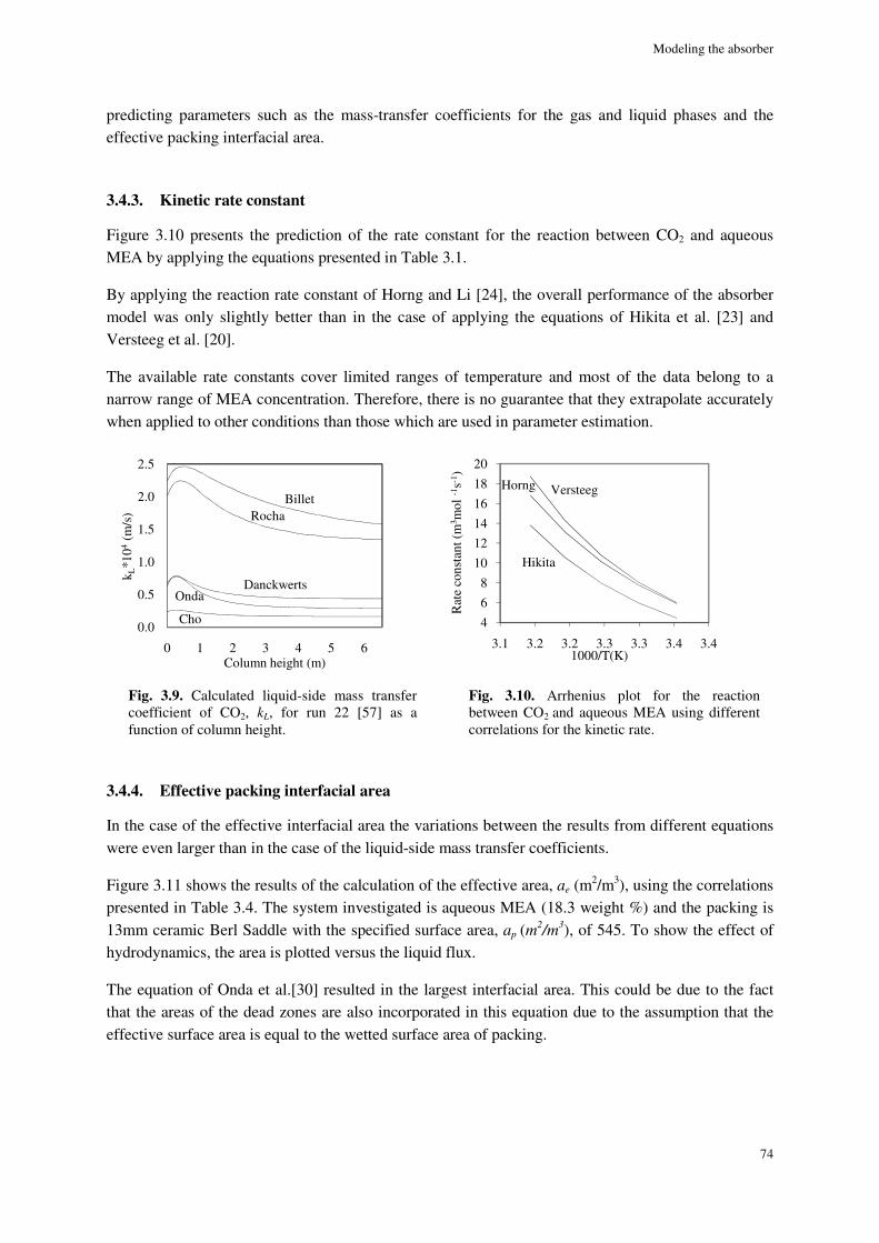
Modeling the absorber
74
predicting parameters such as the mass-transfer coefficients for the gas and liquid phases and the effective packing interfacial area.
3.4.3. Kinetic rate constant
Figure 3.10 presents the prediction of the rate constant for the reaction between CO2 and aqueous MEA by applying the equations presented in Table 3.1.
By applying the reaction rate constant of Horng and Li [24], the overall performance of the absorber model was only slightly better than in the case of applying the equations of Hikita et al. [23] and Versteeg et al. [20].
The available rate constants cover limited ranges of temperature and most of the data belong to a narrow range of MEA concentration. Therefore, there is no guarantee that they extrapolate accurately when applied to other conditions than those which are used in parameter estimation.
3.4.4. Effective packing interfacial area
In the case of the effective interfacial area the variations between the results from different equations were even larger than in the case of the liquid-side mass transfer coefficients.
Figure 3.11 shows the results of the calculation of the effective area, ae (m2/m3), using the correlations
presented in Table 3.4. The system investigated is aqueous MEA (18.3 weight %) and the packing is 13mm ceramic Berl Saddle with the specified surface area, ap (m
2/m
3), of 545. To show the effect of hydrodynamics, the area is plotted versus the liquid flux.
The equation of Onda et al.[30] resulted in the largest interfacial area. This could be due to the fact that the areas of the dead zones are also incorporated in this equation due to the assumption that the effective surface area is equal to the wetted surface area of packing.
0.0
0.5
1.0
1.5
2.0
2.5
0 1 2 3 4 5 6
k L*1
04(m
/s)
Column height (m)
BilletRocha
Danckwerts Onda
Cho 4
6
8
10
12
14
16
18
20
3.1 3.2 3.2 3.3 3.3 3.4 3.4
Rat
e co
nsta
nt (
m3 m
ol -1
s-1)
1000/T(K)
VersteegHorng
Hikita
Fig. 3.9. Calculated liquid-side mass transfer coefficient of CO2, kL, for run 22 [57] as a function of column height.
Fig. 3.10. Arrhenius plot for the reaction between CO2 and aqueous MEA using different correlations for the kinetic rate.
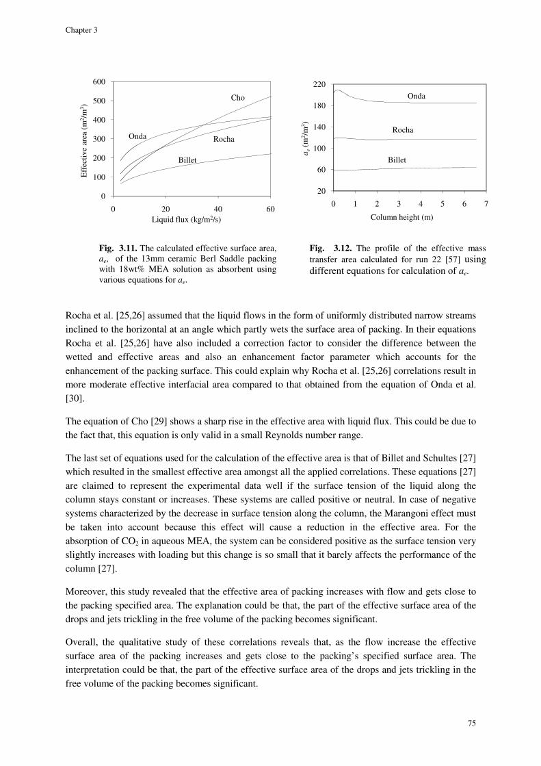
Chapter 3
75
Rocha et al. [25,26] assumed that the liquid flows in the form of uniformly distributed narrow streams inclined to the horizontal at an angle which partly wets the surface area of packing. In their equations Rocha et al. [25,26] have also included a correction factor to consider the difference between the wetted and effective areas and also an enhancement factor parameter which accounts for the enhancement of the packing surface. This could explain why Rocha et al. [25,26] correlations result in more moderate effective interfacial area compared to that obtained from the equation of Onda et al. [30].
The equation of Cho [29] shows a sharp rise in the effective area with liquid flux. This could be due to the fact that, this equation is only valid in a small Reynolds number range.
The last set of equations used for the calculation of the effective area is that of Billet and Schultes [27]
which resulted in the smallest effective area amongst all the applied correlations. These equations [27] are claimed to represent the experimental data well if the surface tension of the liquid along the column stays constant or increases. These systems are called positive or neutral. In case of negative systems characterized by the decrease in surface tension along the column, the Marangoni effect must be taken into account because this effect will cause a reduction in the effective area. For the absorption of CO2 in aqueous MEA, the system can be considered positive as the surface tension very slightly increases with loading but this change is so small that it barely affects the performance of the column [27].
Moreover, this study revealed that the effective area of packing increases with flow and gets close to the packing specified area. The explanation could be that, the part of the effective surface area of the drops and jets trickling in the free volume of the packing becomes significant.
Overall, the qualitative study of these correlations reveals that, as the flow increase the effective surface area of the packing increases and gets close to the packing’s specified surface area. The interpretation could be that, the part of the effective surface area of the drops and jets trickling in the free volume of the packing becomes significant.
Fig. 3.11. The calculated effective surface area, ae, of the 13mm ceramic Berl Saddle packing with 18wt% MEA solution as absorbent using various equations for ae.
0
100
200
300
400
500
600
0 20 40 60
Eff
ectiv
e ar
ea (
m2 /
m3 )
Liquid flux (kg/m2/s)
Onda
Billet
Cho
Rocha
20
60
100
140
180
220
0 1 2 3 4 5 6 7
ae
(m2 /
m3 )
Column height (m)
Rocha
Billet
Onda
Fig. 3.12. The profile of the effective mass transfer area calculated for run 22 [57] using different equations for calculation of ae.
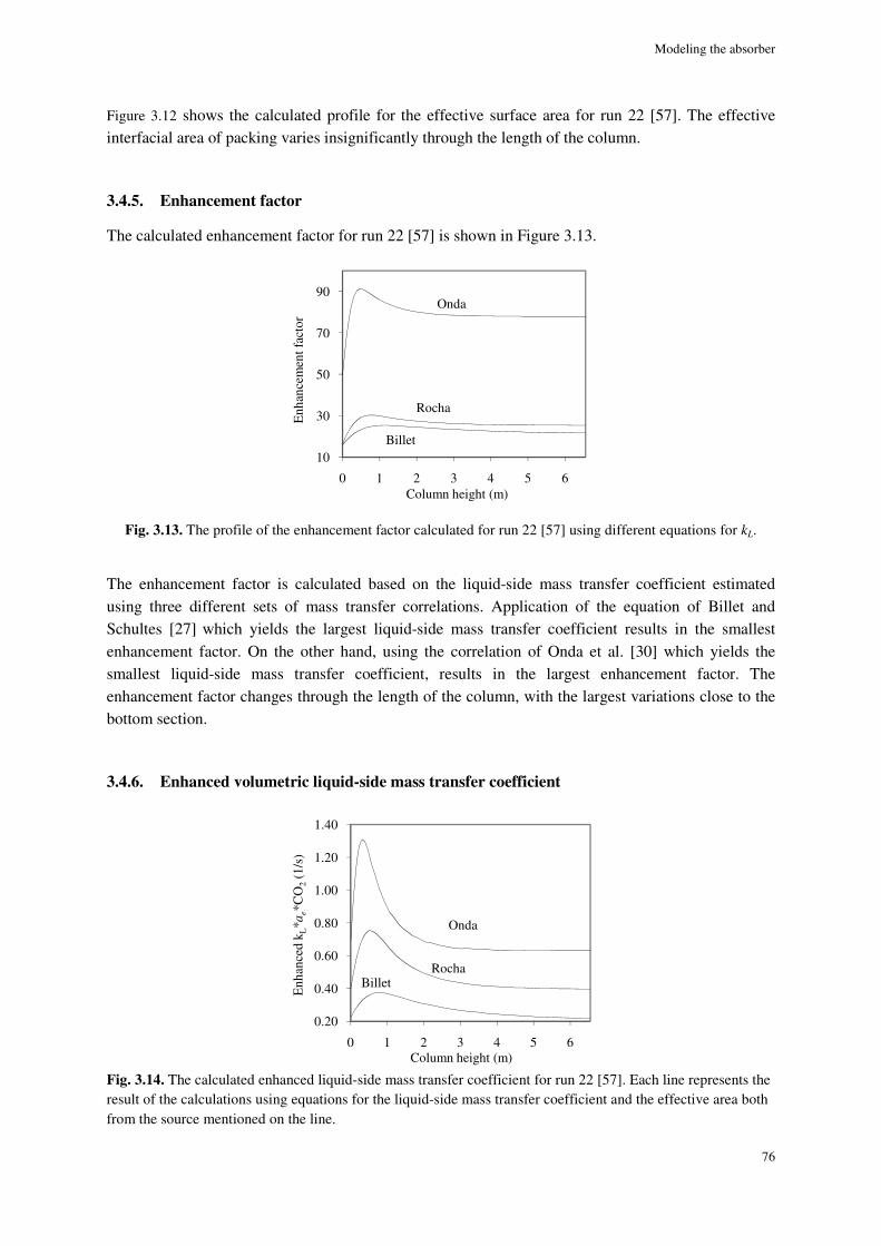
Modeling the absorber
76
Figure 3.12 shows the calculated profile for the effective surface area for run 22 [57]. The effective interfacial area of packing varies insignificantly through the length of the column.
3.4.5. Enhancement factor
The calculated enhancement factor for run 22 [57] is shown in Figure 3.13.
Fig. 3.13. The profile of the enhancement factor calculated for run 22 [57] using different equations for kL.
The enhancement factor is calculated based on the liquid-side mass transfer coefficient estimated using three different sets of mass transfer correlations. Application of the equation of Billet and Schultes [27] which yields the largest liquid-side mass transfer coefficient results in the smallest enhancement factor. On the other hand, using the correlation of Onda et al. [30] which yields the smallest liquid-side mass transfer coefficient, results in the largest enhancement factor. The enhancement factor changes through the length of the column, with the largest variations close to the bottom section.
3.4.6. Enhanced volumetric liquid-side mass transfer coefficient
Fig. 3.14. The calculated enhanced liquid-side mass transfer coefficient for run 22 [57]. Each line represents the result of the calculations using equations for the liquid-side mass transfer coefficient and the effective area both from the source mentioned on the line.
10
30
50
70
90
0 1 2 3 4 5 6
Enh
ance
men
t fac
tor
Column height (m)
Billet
Rocha
Onda
0.20
0.40
0.60
0.80
1.00
1.20
1.40
0 1 2 3 4 5 6
Enh
ance
d k L
*ae*C
O2
(1/s
)
Column height (m)
Onda
BilletRocha
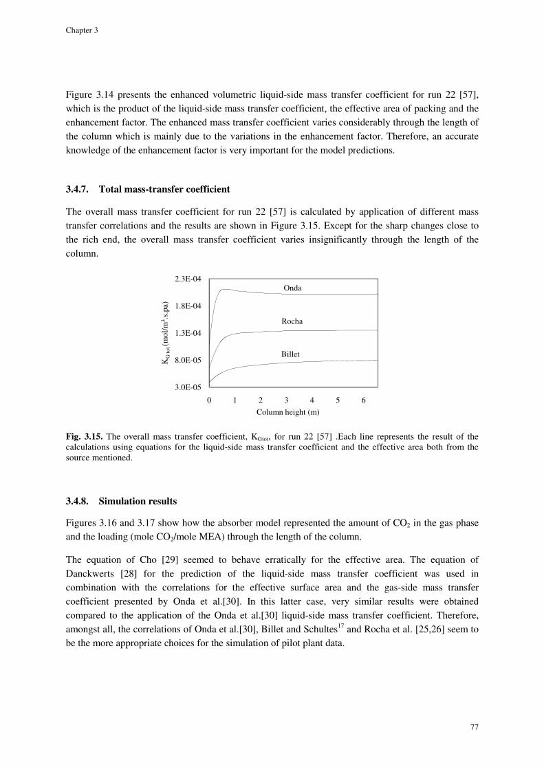
Chapter 3
77
Figure 3.14 presents the enhanced volumetric liquid-side mass transfer coefficient for run 22 [57], which is the product of the liquid-side mass transfer coefficient, the effective area of packing and the enhancement factor. The enhanced mass transfer coefficient varies considerably through the length of the column which is mainly due to the variations in the enhancement factor. Therefore, an accurate knowledge of the enhancement factor is very important for the model predictions.
3.4.7. Total mass-transfer coefficient
The overall mass transfer coefficient for run 22 [57] is calculated by application of different mass transfer correlations and the results are shown in Figure 3.15. Except for the sharp changes close to the rich end, the overall mass transfer coefficient varies insignificantly through the length of the column.
Fig. 3.15. The overall mass transfer coefficient, KGtot, for run 22 [57] .Each line represents the result of the calculations using equations for the liquid-side mass transfer coefficient and the effective area both from the source mentioned.
3.4.8. Simulation results
Figures 3.16 and 3.17 show how the absorber model represented the amount of CO2 in the gas phase and the loading (mole CO2/mole MEA) through the length of the column.
The equation of Cho [29] seemed to behave erratically for the effective area. The equation of Danckwerts [28] for the prediction of the liquid-side mass transfer coefficient was used in combination with the correlations for the effective surface area and the gas-side mass transfer coefficient presented by Onda et al.[30]. In this latter case, very similar results were obtained compared to the application of the Onda et al.[30] liquid-side mass transfer coefficient. Therefore, amongst all, the correlations of Onda et al.[30], Billet and Schultes17 and Rocha et al. [25,26] seem to be the more appropriate choices for the simulation of pilot plant data.
3.0E-05
8.0E-05
1.3E-04
1.8E-04
2.3E-04
0 1 2 3 4 5 6
KG
tot (
mol
/m3 .
s.pa
)
Column height (m)
Rocha
Billet
Onda
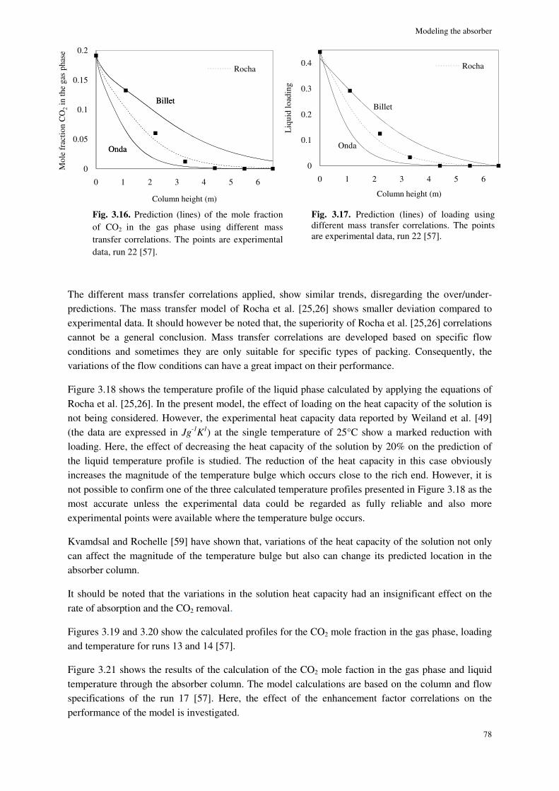
Modeling the absorber
78
The different mass transfer correlations applied, show similar trends, disregarding the over/under-predictions. The mass transfer model of Rocha et al. [25,26] shows smaller deviation compared to experimental data. It should however be noted that, the superiority of Rocha et al. [25,26] correlations cannot be a general conclusion. Mass transfer correlations are developed based on specific flow conditions and sometimes they are only suitable for specific types of packing. Consequently, the variations of the flow conditions can have a great impact on their performance.
Figure 3.18 shows the temperature profile of the liquid phase calculated by applying the equations of Rocha et al. [25,26]. In the present model, the effect of loading on the heat capacity of the solution is not being considered. However, the experimental heat capacity data reported by Weiland et al. [49] (the data are expressed in Jg
-1K
1) at the single temperature of 25°C show a marked reduction with loading. Here, the effect of decreasing the heat capacity of the solution by 20% on the prediction of the liquid temperature profile is studied. The reduction of the heat capacity in this case obviously increases the magnitude of the temperature bulge which occurs close to the rich end. However, it is not possible to confirm one of the three calculated temperature profiles presented in Figure 3.18 as the most accurate unless the experimental data could be regarded as fully reliable and also more experimental points were available where the temperature bulge occurs.
Kvamdsal and Rochelle [59] have shown that, variations of the heat capacity of the solution not only can affect the magnitude of the temperature bulge but also can change its predicted location in the absorber column.
It should be noted that the variations in the solution heat capacity had an insignificant effect on the rate of absorption and the CO2 removal.
Figures 3.19 and 3.20 show the calculated profiles for the CO2 mole fraction in the gas phase, loading and temperature for runs 13 and 14 [57].
Figure 3.21 shows the results of the calculation of the CO2 mole faction in the gas phase and liquid temperature through the absorber column. The model calculations are based on the column and flow specifications of the run 17 [57]. Here, the effect of the enhancement factor correlations on the performance of the model is investigated.
0
0.05
0.1
0.15
0.2
0 1 2 3 4 5 6
Mol
e fr
actio
n C
O2
in th
e ga
s ph
ase
Column height (m)
Rocha
Billet
Onda
Billet
Onda
0
0.1
0.2
0.3
0.4
0 1 2 3 4 5 6
Liq
uid
load
ing
Column height (m)
Rocha
Billet
Onda
Fig. 3.16. Prediction (lines) of the mole fraction of CO2 in the gas phase using different mass transfer correlations. The points are experimental data, run 22 [57].
Fig. 3.17. Prediction (lines) of loading using different mass transfer correlations. The points are experimental data, run 22 [57].
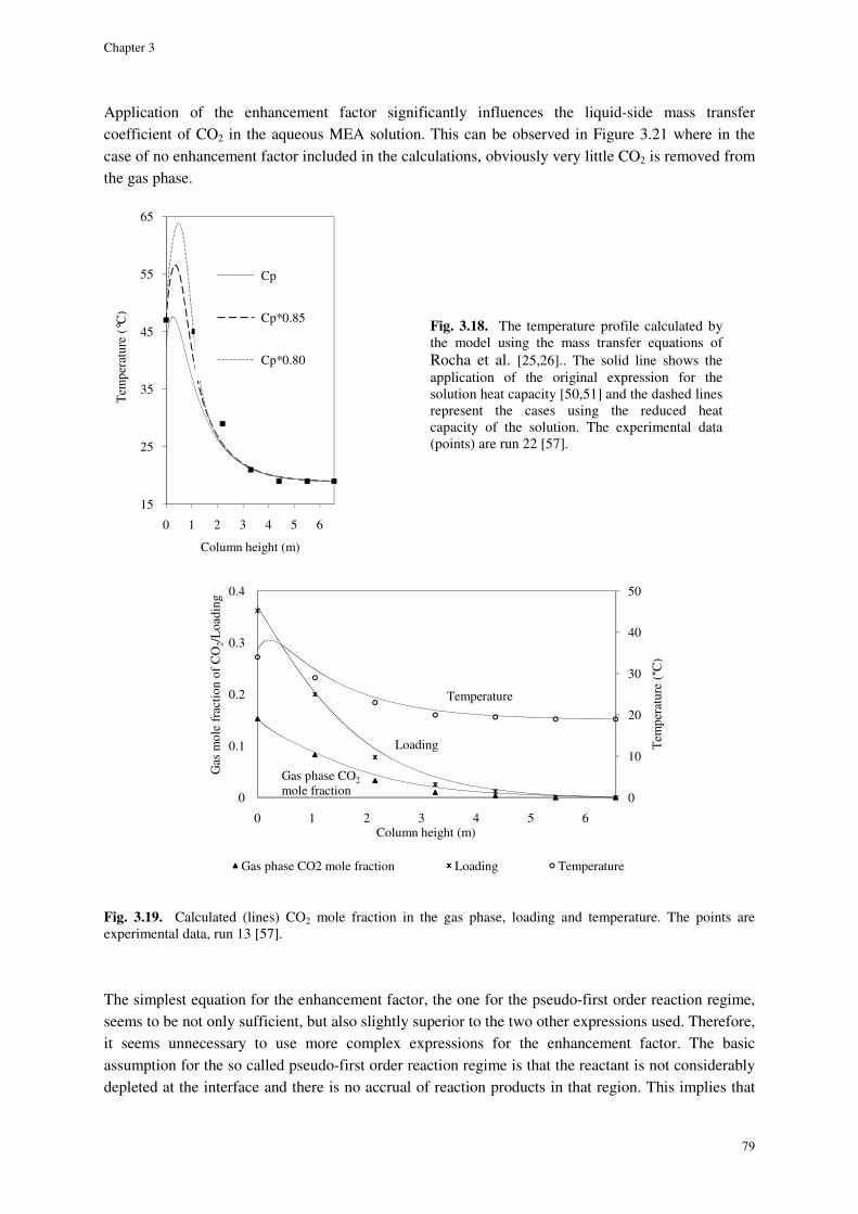
Chapter 3
79
Application of the enhancement factor significantly influences the liquid-side mass transfer coefficient of CO2 in the aqueous MEA solution. This can be observed in Figure 3.21 where in the case of no enhancement factor included in the calculations, obviously very little CO2 is removed from the gas phase.
Fig. 3.19. Calculated (lines) CO2 mole fraction in the gas phase, loading and temperature. The points are experimental data, run 13 [57].
The simplest equation for the enhancement factor, the one for the pseudo-first order reaction regime, seems to be not only sufficient, but also slightly superior to the two other expressions used. Therefore, it seems unnecessary to use more complex expressions for the enhancement factor. The basic assumption for the so called pseudo-first order reaction regime is that the reactant is not considerably depleted at the interface and there is no accrual of reaction products in that region. This implies that
15
25
35
45
55
65
0 1 2 3 4 5 6
Tem
pera
ture
(°C
)
Column height (m)
Cp
Cp*0.85
Cp*0.80
0
10
20
30
40
50
0
0.1
0.2
0.3
0.4
0 1 2 3 4 5 6
Gas
mol
e fr
actio
n of
CO
2/L
oadi
ng
Column height (m)
Gas phase CO2 mole fraction Loading Temperature
Loading
Gas phase CO2mole fraction
Tem
pera
ture
(°C
)
Temperature
Fig. 3.18. The temperature profile calculated by the model using the mass transfer equations of Rocha et al. [25,26].. The solid line shows the application of the original expression for the solution heat capacity [50,51] and the dashed lines represent the cases using the reduced heat capacity of the solution. The experimental data (points) are run 22 [57].
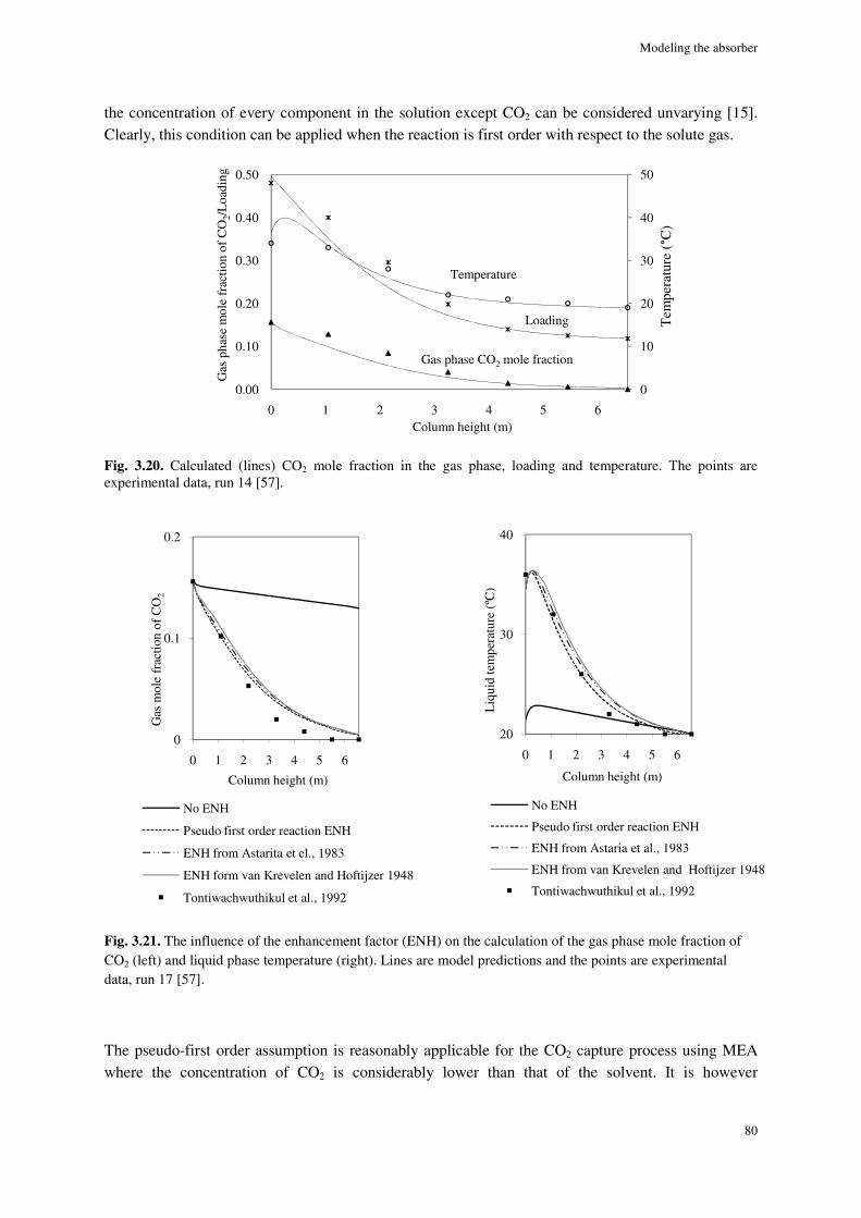
Modeling the absorber
80
the concentration of every component in the solution except CO2 can be considered unvarying [15]. Clearly, this condition can be applied when the reaction is first order with respect to the solute gas.
Fig. 3.20. Calculated (lines) CO2 mole fraction in the gas phase, loading and temperature. The points are experimental data, run 14 [57].
Fig. 3.21. The influence of the enhancement factor (ENH) on the calculation of the gas phase mole fraction of CO2 (left) and liquid phase temperature (right). Lines are model predictions and the points are experimental data, run 17 [57].
The pseudo-first order assumption is reasonably applicable for the CO2 capture process using MEA where the concentration of CO2 is considerably lower than that of the solvent. It is however
0
10
20
30
40
50
0.00
0.10
0.20
0.30
0.40
0.50
0 1 2 3 4 5 6
Gas
pha
se m
ole
frac
tion
of C
O2/
Loa
ding
Column height (m)
Tem
pera
ture
(°C
)
Temperature
Loading
Gas phase CO2 mole fraction
0
0.1
0.2
0 1 2 3 4 5 6
Gas
mol
e fr
actio
n of
CO
2
Column height (m)
No ENH
Pseudo first order reaction ENH
ENH from Astarita et el., 1983
ENH form van Krevelen and Hoftijzer 1948
Tontiwachwuthikul et al., 1992
20
30
40
0 1 2 3 4 5 6
Liq
uid
tem
pera
ture
(ºC
)
Column height (m)
No ENH
Pseudo first order reaction ENH
ENH from Astaria et al., 1983
ENH from van Krevelen and Hoftijzer 1948
Tontiwachwuthikul et al., 1992
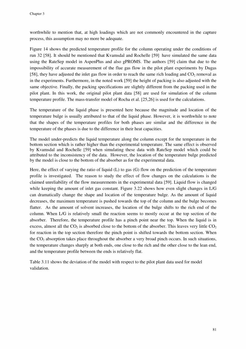
Chapter 3
81
worthwhile to mention that, at high loadings which are not commonly encountered in the capture process, this assumption may no more be adequate.
Figure 14 shows the predicted temperature profile for the column operating under the conditions of run 32 [58]. It should be mentioned that Kvamsdal and Rochelle [59] have simulated the same data using the RateSep model in AspenPlus and also gPROMS. The authors [59] claim that due to the
impossibility of accurate measurement of the flue gas flow in the pilot plant experiments by Dugas [58], they have adjusted the inlet gas flow in order to reach the same rich loading and CO2 removal as in the experiments. Furthermore, in the noted work [59] the height of packing is also adjusted with the same objective. Finally, the packing specifications are slightly different from the packing used in the pilot plant. In this work, the original pilot plant data [58] are used for simulation of the column temperature profile. The mass-transfer model of Rocha et al. [25,26] is used for the calculations.
The temperature of the liquid phase is presented here because the magnitude and location of the temperature bulge is usually attributed to that of the liquid phase. However, it is worthwhile to note that the shapes of the temperature profiles for both phases are similar and the difference in the temperature of the phases is due to the difference in their heat capacities.
The model under-predicts the liquid temperature along the column except for the temperature in the bottom section which is rather higher than the experimental temperature. The same effect is observed by Kvamsdal and Rochelle [59] when simulating these data with RateSep model which could be attributed to the inconsistency of the data. However, the location of the temperature bulge predicted by the model is close to the bottom of the absorber as for the experimental data.
Here, the effect of varying the ratio of liquid (L) to gas (G) flow on the prediction of the temperature profile is investigated. The reason to study the effect of flow changes on the calculations is the claimed unreliability of the flow measurements in the experimental data [59]. Liquid flow is changed while keeping the amount of inlet gas constant. Figure 3.22 shows how even slight changes in L/G can dramatically change the shape and location of the temperature bulge. As the amount of liquid decreases, the maximum temperature is pushed towards the top of the column and the bulge becomes flatter. As the amount of solvent increases, the location of the bulge shifts to the rich end of the column. When L/G is relatively small the reaction seems to mostly occur at the top section of the absorber. Therefore, the temperature profile has a pinch point near the top. When the liquid is in excess, almost all the CO2 is absorbed close to the bottom of the absorber. This leaves very little CO2 for reaction in the top section therefore the pinch point is shifted towards the bottom section. When the CO2 absorption takes place throughout the absorber a very broad pinch occurs. In such situations, the temperature changes sharply at both ends, one close to the rich and the other close to the lean end, and the temperature profile between the ends is relatively flat.
Table 3.11 shows the deviation of the model with respect to the pilot plant data used for model validation.
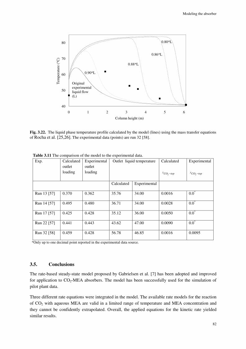
Modeling the absorber
82
Fig. 3.22. The liquid phase temperature profile calculated by the model (lines) using the mass transfer equations of Rocha et al. [25,26]. The experimental data (points) are run 32 [58].
Table 3.11 The comparison of the model to the experimental data. Exp. Calculated
outlet loading
Experimental outlet loading
Outlet liquid temperature Calculated
2yCO top−
Experimental
2yCO top−
Calculated Experimental
Run 13 [57] 0.370 0.362 35.76 34.00 0.0016 0.0*
Run 14 [57] 0.495 0.480 36.71 34.00 0.0028 0.0*
Run 17 [57] 0.425 0.428 35.12 36.00 0.0050 0.0*
Run 22 [57] 0.441 0.443 43.62 47.00 0.0090 0.0*
Run 32 [58] 0.459 0.428 56.78 46.85 0.0016 0.0095
*Only up to one decimal point reported in the experimental data source.
3.5. Conclusions
The rate-based steady-state model proposed by Gabrielsen et al. [7] has been adopted and improved for application to CO2-MEA absorbers. The model has been successfully used for the simulation of pilot plant data.
Three different rate equations were integrated in the model. The available rate models for the reaction of CO2 with aqueous MEA are valid in a limited range of temperature and MEA concentration and they cannot be confidently extrapolated. Overall, the applied equations for the kinetic rate yielded similar results.
40
50
60
70
80
0 1 2 3 4 5 6
Tem
pera
ture
(°C
)
Column height (m)
Original experimental liquid flow (L)
0.90*L
0.80*L
0.86*L
0.88*L
Chapter 3
83
The accuracy of the model’s predictions are dependent on the mass transfer correlations applied. The mass transfer model of Rocha et al. [25,26] showed smaller deviation compared to experimental data for the cases investigated. However, mass transfer correlations are developed based on specific flow conditions and sometimes they are only suitable for specific types of packing. Consequently, these models may not be accurate at all hydrodynamic conditions.
The enhancement factor for the pseudo-first order reaction seemed to be not only sufficient, but the preferred approach for representing the experimental data for the loading ranges considered.
Overall, the simple model for the CO2 absorber packed column proposed is a valuable tool for simulating the capture process. In cases where the quality of the essential fundamental data is dubious and the available correlations for the basic properties are not fully reliable, a simple model for CO2 absorber design is a suitable approach.
List of symbols
ae effective specific interfacial area, 1/m ap packing specific surface area, 1/m C packing specific constant D diffusion coefficient, m2/s
dh hydraulic diameter of packing defined by 4
pa
ε , m
dp particle diameter, m E enhancement factor E∞ enhancement factor for the instantaneous reaction Fse packing surface enhancement factor Ft correction factor for total liquid holdup
FrL Froude number for the liquid,2L pu a
g
g gravitational constant, m/s2 He Henry’s law constant, Pa.m3/mol hL liquid holdup, m3/m3 K proportionality constant for the N2O analogy k kinetic rate constant, m3mol-1s-1 kG gas-side mass transfer coefficient, m/s kL liquid-side mass transfer coefficient, m/s L superficial mass velocity of liquid, kg/m2. hr
ReL Reynolds number for liquid defined by
except when used in the mass transfer equations of
Onda et al.[30] for which the definition for Reynolds number is included in Table 4. S side dimension of corrugation, m
ScL Schmidt number for liquid defined by
sr surface renewal rate T temperature (K) u superficial velocity, m/s
WeL Weber number for the liquid defined by
Greek letters
α corrugation inclination angle σ surface tension, N/m ε void fraction of packing
Modeling the absorber
84
ѳ contact angle µ viscosity, kg/(m.s) ν kinematic viscosity, m2/s ρ density, kg/m3
Subscripts
c critical e effective G gas L liquid neu neutral pos positive
References
[1] PV. Danckwerts, E. Alper, Trans. Inst. Chem. Eng. 1 (1975) 34-40. [2] L. De Leye, G. F. Forment, Comput. Chem. Eng. 10 (1986) 493-504. [3] J. D. Pandya, Chem. Eng. Commun. 19 (1983) 343-361. [4] L. Kucka, I. Muller, E. Y. Kenig, A. Gorak, Chem. Eng. Sci. 58 (2003) 3571-3578. [5] I. Alatiqi, M. F. Sabri, W. Bouhamra, E. Alper, Gas Sep. Purif. 8 (1994) 3-11. [6] Tobiesen, F. A.; Svendsen, H. F.; Juliussen, O., AIChE J. 53 (2007) 846-865. [7] J. Gabrielsen, M. L. Michelsen, E. H. Stenby, G. M. Kontogeorgis, AIChE J. 52 (2006) 3443-3451. [8] G. Astarita, D. W. Savage, A. Bisio, Gas Treating with Chemical Solvents. Wiley: New York, 1983. [9] L. F. Shampine, P. H. Muir, H. Xu, JNAIAM 1 (2006) 201-217. [10] W. P. M. van Swaaij, G. F. Versteeg, Chem. Eng. Sci. 47 (13/14) (1992) 3181-3195
[11] L. Kucka, E. Y. Kenig, A. Górak, Ind. Eng. Chem. Res. 41 (2002) 5952-5957. [12] W. K. Lewis, W. G. Whitman, Ind. Eng. Chem. 16 (12) (1924). [13] PV. Danckwerts, Gas-Liquid Reactions, McGraw-Hill, New York, 1970. [14] G.T. Rochelle, S. Bishnoi, S. Chi, H. Dang, J. Santos, Final report for P.O. No. DE-AF26-99FT01029, US Department of Energy, Federal Energy Technology Center, Pittsburgh, 2001. [15] S. Freguia S., MSc Thesis, The University of Texas at Austin, 2002. [16] Gabrielsen J., PhD Thesis, Technical University of Denmark, 2007. [17] D. W. van Krevelen, P. J. Hoftijzer, Rec. Trav. Chim. 67 (1948) 563-586. [18] L. Kucka, J. Richter, E. Y. Kenig, A. Gorak, Sep. Purif. Technol. 31 (2003) 163-175. [19] V. V. Mahajani, J. B. Joshi, Gas Sep. Purif. 2 (1988) 50-64. [20] G. F. Versteeg, L. van Dijck, W. P. M. van Swaaij, Chem. Eng. Commun. 144 (1996) 113-158. [21] A. Aboudheir, P. Tontiwachwuthikul, A. Chakma, R. Idem, Chem. Eng. Sci. 58 (2003) 5159-5210. [22] P.D. Vaidya, E.Y. Kenig, Chem. Eng. Technol. 30 (2007) 1467-1474. [23] H. Hikita, S. Asai, H. Ishikawa, M. Honda, Chem. Eng. J. 13 (1977) 7-12. [24] S-Y Horng, M-H Li, Ind. Eng. Chem. Res. 41 (2002) 257-266. [25] J. A. Rocha, J. L.Bravo, J. R. Fair, Ind. Eng. Chem. Res. 32 (1993) 641-651. [26] J. A. Rocha, J. L.Bravo, J. R. Fair, Ind. Eng. Chem. Res. 35 (1996) 1660-1667. [27] R. Billet, R., M. Schultes, Trans. IChemE. 77 (1999) 498-504. [28] P. V. Danckwerts, A. M. Kennedy, Trans. Inst. Chem. Engrs. 32 (1954) 53. [29] J. S. Cho, PhD Thesis, Oregon State University, 1987. [30] K. Onda, K., H. Takeuchi, Y. Okumoto, J. Chem. Eng. Jpn. 1 (1968) 56-62. [31] N. Kolev, S. Nakov, L. Ljutzkanov, D. Kolev, Chem. Eng. Process. 45 (2006) 429-436. [32] G. Q. Wang, X. G. Yuan, K. T. Yu, Ind. Eng. Chem. Res. 44 (2005) 8715-8729. [33]M. G. Shi, A. Mersmann, Ger. Chem. Eng. 8 (1985) 87-96. [34] R. H. Weiland, A Joint Research Report by the Gas Processors Association and the Gas Research Institute, Research Report RR-152, GPA Project 911, 1996. [35] D. W. van Krevelen, P. J. Hoftijzer, Chem. Eng. Prog. 44 (1948) 529-536. [36] G. J. Browning, R. H. Weiland, J. Chem. Eng. Data 39 (1994) 817-822. [37] P. V. Danckwerts, M. M. Sharma M. M., Chem. Eng. Sci. 44 (1996) 244-280. [38] N. Haimour, O. C. Sandall, Chem. Eng. Sci. 39 (12) (1984) 1791-1796. [39] H. A. Al-Ghawas, D. P. Hagewiesche, G. Ruiz-Ibanez, O.C. Sandall, J. Chem. Eng. Data 34 (1989) 385-391. [40] M. H. Li, W. C. Lee W.C., J. Chem. Eng. Data 41 (3) (1996) 551-556. [41] G. F. Versteeg, W. P. M. van Swaaij, J. Chem. Eng. Data 33 (1988) 29-34. [42] T. C. Tsai, J. J. Ko, H. M. Wang, C. Y. Lin, M. H. Li, J. Chem. Eng. Data 45 (2) (2000) 341-347. [43] B. P. Mandal, M. Kundu, N. U. Padhiyar, S. S. Bandyopadhyay, J. Chem. Eng. Data 49 (2) (2004) 264-270. [44] B. P. Mandal, M. Kundu, S. S. Bandyopadhyay, J. Chem. Eng. Data 50 (2005) 352-358. [45] J. K. A. Clarke, Ind. And CE Fundamentals, 3 (3) (1964) 239-245. [46] E. Sada, H. Kumazawa, M. Butt, J. Chem. Eng. Data 23 (2) (1978) 161-164.

Chapter 3
85
[47] J-J Ko, T-C Tsai, C-Y Lin, H-M Wang, M-H Li, J. Chem. Eng. Data 46 (2001) 160-165. [48] G. Vázquez, E. Alvarez, J. M. Navaza, R. Rendo, E. Romero, J. Chem. Eng. Data 42 (1997) 57-59. [49] R. H. Weiland, J. C. Dingman, D. B. Cronin, J. Chem. Eng. Data 42 (1997) 1004-1006. [50] M. Mundhwa, R. Alam, A. Henni, J. Chem. Eng. Data 51 (2006) 491-498. [51] N. S. Osborne, H. F. Stimson, D. C. Ginnings, J. Res. Natl. Bur. Standards 23 (1939) 197-260. [52] R. C. Reid, J. M. Prausnitz, B. E. Poling, The Properties of Gases and Liquids. 4th Edition. New York: McGraw-Hill, 1987. [53] C-H Hsu, M-H Li, J. Chem. Eng. Data 42 (1997) 502-507. [54] Y. W. Wang, S. Xu, F. D. Otto, A. E. Mather, Chem. Eng. J. Biochem. Eng. J. 48 (1992) 31-40. [55] E . D. Snijder, J. M. te Riele, G. F. Versteeg, W. P. M. van Swaaji, J. Chem. Eng. Data 38 (1993) 475-480. [56] J. Gabrielsen, M. L. Michelsen, E. H. Stenby, G. M. Kontogeorgis, Ind. Eng. Chem. Res. 44 (2005) 3348-3354. [57] P. Tontiwachwuthikul, A. Meisen, C. J. Lim, Chem. Eng. Sci. 47 (1992) 381-390. [58] R. E. Dugas, MSE Thesis, The University of Texas at Austin, 2006. [59] H. M. Kvamsdal, G. T. Rochelle, Ind. Eng. Chem. Res. 47 (2008) 867-875. [60] W. McCabe, J. Smith, P. Harriott, Unit Operations of Chemical Engineering. 6th Edition, McGraw-Hill, 2000. [61] L. Faramarzi, G. M. Kontogeorgis, M. L. Michelsen, K. Thomsen, E. H. Stenby, Ind. Eng. Chem. Res. 49 (2010) 3751-3759.

44
NUMERICAL IMPLEMENTATION OF THE ABSORBER MODEL
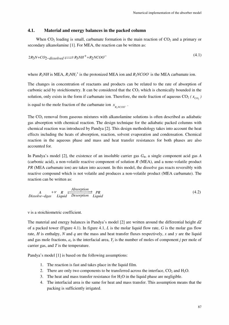
Numerical implementation of the absorber model
87
4.1. Material and energy balances in the packed column
When CO2 loading is small, carbamate formation is the main reaction of CO2 and a primary or secondary alkanolamine [1]. For MEA, the reaction can be written as:
(4.1)
where R2NH is MEA, R3NH3+ is the protonized MEA ion and R2NCOO
- is the MEA carbamate ion.
The changes in concentration of reactants and products can be related to the rate of absorption of carbonic acid by stoichiometry. It can be considered that the CO2 which is chemically bounded in the
solution, only exists in the form if carbamate ion. Therefore, the mole fraction of aqueous CO2 (2CO
x )
is equal to the mole fraction of the carbamate ion 2R NCOO
x − .
The CO2 removal from gaseous mixtures with alkanolamine solutions is often described as adiabatic gas absorption with chemical reaction. The design technique for the adiabatic packed columns with chemical reaction was introduced by Pandya [2]. This design methodology takes into account the heat effects including the heats of absorption, reaction, solvent evaporation and condensation. Chemical reaction in the aqueous phase and mass and heat transfer resistances for both phases are also accounted for.
In Pandya’s model [2], the existence of an insoluble carrier gas GB, a single component acid gas A (carbonic acid), a non-volatile reactive component of solution R (MEA), and a none-volatile product PR (MEA carbamate ion) are taken into account. In this model, the dissolve gas reacts reversibly with reactive compound which is not volatile and produces a non-volatile product (MEA carbamate). The reaction can be written as:
AbsorptionA R PR
DesorptionDissolve dgas Liquid Liquidν →←+
− (4.2)
ν is a stoichiometric coefficient.
The material and energy balances in Pandya’s model [2] are written around the differential height dZ of a packed tower (Figure 4.1). In figure 4.1, L is the molar liquid flow rate, G is the molar gas flow rate, H is enthalpy, N and q are the mass and heat transfer fluxes respectively, x and y are the liquid and gas mole fractions, ae is the interfacial area, Yj is the number of moles of component j per mole of carrier gas, and T is the temperature.
Pandya’s model [1] is based on the following assumptions:
1. The reaction is fast and takes place in the liquid film. 2. There are only two components to be transferred across the interface, CO2 and H2O. 3. The heat and mass transfer resistance for H2O in the liquid phase are negligible. 4. The interfacial area is the same for heat and mass transfer. This assumption means that the
packing is sufficiently irrigated.
2 3 2 3 2R N CO R NH R NCOOdissolved →←+ −+ +−
Chepter 4
88
5. Axial dispersions are not accounted for due to the fact that these effects are considered to be insignificant.
Fig. 4.1. Differential section of the absorber.
The concentration gradients in each differential section can be presented as:
( )2 2 22
gas bulk interfaceGCO e c CO COCOk a A P y ydy
dz G
− −− −= (4.3)
( )2 2 22
gas bulk interfaceGH O e c H O COH Ok a A P y ydy
dz G
− −− −= (4.4)
where P and kG are the pressure and the mass transfer coefficient for the gas phase respectively and Ac is the cross sectional area of the column.
The temperature gradients in each differential section for the two phases can be written as:
( )( )2 2 2 2
h a A T Te cG G LG
G C Y C Y CB pB CO p pCO H O H O
dT
dZ
− −=
+ + (4.5)
2
2 2 2 2 2
2
0
0 0
( ) ( ( ) )
( ( ) ( , ))
H OG
B pB CO pCO H O pH O B pH O G s
Z
B pCO G RL
pL
dYdTG C Y C Y C G C T T
dT dZ
G C T T H T PdT
dZ LC
λ+ + + − + +
− − ∆=
(4.6)
G+dG,
Yj+dYj,
yj+dyj,
TG+dTG
HG+dHG
Interface surface = ae*dZ
G,Yj, yj,TG, HG
dZ
L+dL,
xj+dxj,
TL+dTL
HL+dHL
L, xj,TL, HL
Gas Ni
qi
Liquid
Ni
qi
Numerical implementation of the absorber model
89
where hG, Cp, λH2O, and RH∆ are the heat transfer coefficient, the heat capacity, the latent heat of
vaporization and the heat of chemical reaction between the absorbed gas and the amine respectively. The subscript B indicates the carrier gas and T0 indicates the reference temperature.
In each differential section, resulting from the mass flux balance equations, the partial pressure of CO2 at the interface can be written as:
2
2 2
2
2
2
2
,
- -
,
CO -interface,
,
1
L CO
CO gas bulk CO eq
G CO
L CO
G CO
k EP C
kP
k E
k He
=
+
+
(4.7)
And the liquid phase mole fraction can be expressed as:
2
2
interfaceinterface
CO
CO
PC
He
−
− = (4.8)
where 2CO eq
C − , He, kL and E are the equilibrium concentration, the Henry’s law constant, the physical
mass transfer coefficient and the enhancement factor, respectively.
Equations 4.6 and 4.7 defined by the model are solved simultaneously to calculate composition and temperature profile along the column. The details of the differential equations of the model and the way they are solved are fully documented in Gabreilsen [3], Tontiwachwuthikul et al. [4] and Pandya [2], therefore they are not repeated here.
The physicho-chemical data required by the simulation model were earlier presented in chapter 3. The vapor-liquid equilibrium data of the absorption system at the inlet and outlet liquid streams are calculated by the VLE model. The reaction rate of CO2 absorption is calculated using the kinetic models introduced in chapter 3. Finally, the physical properties of the gas and the liquid phases are calculated using the appropriate correlations found in the open literature as presented in the previous chapter.
List of symbols
A dissolved gas ae effective specific interfacial area, 1/m Ac cross sectional area of the column, m2
B carrier gas E enhancement factor kG gas-side mass transfer coefficient, mol/m2.s.pa kL liquid-side mass transfer coefficient, m/s C concentration, mol/m3
CP molar heat capacity, J/mol.K G molar gas flow, mol/s h heat transfer coefficient in gas, J/s.K.m2 He Henry’s law constant, Pa.m3/mol H Heat of reaction, J/mol L molar flow, mol/s N molar flux, mol/m2.s
Chepter 4
90
P pressure, kPa PR reaction product, nonvolatile q heat flux, J/m2.s R reactive component of the solution, nonvolatile T Temperature, K
x liquid phase mole fraction y gas phase mole fraction Y number of moles of a gas component/mole of carrier gas Z height of packing, m
Greek letters
λ latent heat of vaporization, J/mol ν stoichiometric coefficient
Subscripts
B carrier gas e effective G gas L liquid 0 reference state
References
[1] G. Astarita, D. W. Savage, A. Bisio, Gas Treating with Chemical Solvents. Wiley: New York, 1983. [2] J. D. Pandya, Chem. Eng. Commun. 19 (1983) 343-361. [3] Gabrielsen J., PhD Thesis, Technical University of Denmark, 2007. [4] P. Tontiwachwuthikul, A. Meisen, C. J. Lim, Chem. Eng. Sci. 47 (1992) 381-390.

55
CONCLUSIONS AND FUTURE PROSPECT
"It is no secret that a lot of climate-change research is subject to opinion, that climate
models sometimes disagree even on the signs of the future changes (e.g. drier vs. wetter future
climate). The problem is, only sensational exaggeration makes the kind of story that will get
politicians’ and readers’ attention. So, yes, climate scientists might exaggerate, but in today’s world,
this is the only way to assure any political action and thus more federal financing to reduce the
scientific uncertainty."
Monika Kopacz, atmospheric scientist
Chapter 5
92
5.1. Concluding remarks
5.1.1. On thermodynamic modelling using extended UNIQUAC model
Most of the available thermodynamic properties essential for the design of the carbonic acid capture units were dealt with in this work. Quaternary, ternary and binary VLE, vapor pressure of pure alkanolamines, excess enthalpy, freezing point depression and speciation in the aqueous phase, were all calculated with good precision using only one single set of a rather small number of parameters. The range of temperature and pressure covered is unparalleled compared to the previous modeling attempts.
For the MEA, MDEA and MEA+MDEA systems the temperature range of -20-200ºC and the total pressures of 0-14000kPa were addressed.
It should be highlighted that extended UNIQUAC has correlated an extensive set of data. However, comparing the model predictions to other models can be only justified if the models of interest (and there are tens of them published) have comparable number of parameters and are tuned with the same data. Having said that, in the literature studies performed in this project, no other model claimed to be capable of achieving similar results as the thermodynamic model of the present work.
5.1.2. On modelling the MEA absorber
Following the work of Gabrielsen et al. [1] a MEA absorber model is developed in this work. The main areas which were subject to change compared to the work of Gabrielsen et al. [1] are as follows:
1. A whole new liquid-side physical property package was needed and now it is in place. Some minor changes needed to be done on the gas-side physical property package and they have been pereformed.
2. Various mass-transfer models are applied and a detailed study of the influence of them on the
model’s predictions is carried out. In the work of Gabrielsen et al. [1], only two mass transfer models were included.
The precision of the model’s prediction is dependent on the mass transfer correlations applied. However, it should be emphasized that the mass transfer correlations are developed based on specific flow conditions and sometimes they are only suitable for specific types of packing. As a result, the mass transfer models may not be accurate in all hydrodynamic conditions. 3. Different enhancement factor expressions are applied in the present work. A comparison of the
effect of enhanced mass transfer by the assumption of different reaction regimes is pereformed.
The enhancement factor for the pseudo-first order reaction seemed adequate for representing the experimental data in the loading ranges which are encountered in the capture process.
4. Various rate equations are implemented and compared.
The available rate models for the reaction of CO2 with aqueous MEA cover a small range of temperature and MEA concentration and they cannot be confidently extrapolated. This is an important
Conclusions and future prospect
93
fact to attend to if the same rate equation is used in the calculations of the stripper column where the temperature is significantly higher. In general, the applied equations did not change the overall performance of the column model significantly.
The model has been successfully applied to CO2 absorber packed columns and validated against pilot plant data with good agreement and therefore seems to be an effective tool to be integrated in the simulation packages.
5.2. Challenges and future work
CO2 emission rate cutback is one of the most important global challenges in the years to come. Post-combustion capture technology is regarded as a potential intermediate answer for tackling the problem of climate change. Therefore, collecting scientific information and data and proper understanding of such systems is an indispensible task to be undertaken. In this PhD the aim was to develop accurate, yet simple models for simulating the alkanolamine-based capture units.
What follows summarizes some of the obstructions encountered in this work and some remarks on what during the course of the present work appeared worth to be investigated:
1. One of the most demanding tasks still to be taken on is the accurate VLE measurement of the CO2+ alkanolamine systems. Although, a large body of VLE data is available on such systems, among various sources a considerable inconsistency prevails. The VLE information of the binary alkanolamine systems (MEA+water) is vital for the prediction of the solvent loss due to vaporization and also is very useful for adjusting the parameters of thermodynamic models such as extended UNIQUAC. However, the open literature data of the binary systems are limited. In the case of MEA as it is a comparatively volatile amine, equilibrium partial pressure is also necessary to be measured accurately as a function of loading. This information is also needed to calculate losses. The data on the vapor pressure of MEA over the loaded solutions is scarce in the open literature.
2. To calculate the standard state properties of the alkanolamine ions formed in the aqueous solutions containing CO2, dissociation constants of the protonated MEA and MDEA and also MEA carbamate ion were needed. In this work the standard state properties were eventually determined by fitting to all kinds of experimental data available in the developed parameter regression database. Experimental data are available on the required dissociation constants. However, they cover a narrow range of temperature. To eliminate the uncertainty of the calculations, it is worthwhile that the equilibrium constants are measured at a broader temperature range. Experimental equilibrium constant for the carbamate ion reaction is particularly more important to measure as the reported data are available in a very limited number and their quality is dubious.
3. Accurate information on the heat capacity of the loaded solutions is essential for the calculation of
the temperature profile of the absorber column. Extended UNIQUAC can be used to calculate the heat capacity. However for the MEA solution loaded with CO2, it did not lead to very sensible results. It needs to be noted that the model was applied for the calculation of the heat capacity without being tuned to any data of this type (neither the data of the loaded solutions nor those of the aqueous alkanolamine systems without CO2). The measured data on the CO2 loaded amines
Chapter 5
94
are available in a very small number and for the MEA system they can only be found at 25°C. It is well worth the effort that measurement of the heat capacity of the loaded alkanolamines is carried out. If these data are available, they can be used to tune the parameters of the thermodynamic models such as extended UNIQUAC and consequently the imprecision of the predictions may be reduced.
4. Speciation of the loaded alkanolamine solutions is important for the estimation of kinetics. There is room for more NMR measurements at the temperatures of the capture process.
5. CO2 absorption and desorption kinetics need to be studied further at absorber and stripper
temperature. The experimental data available are mostly relevant to the absorber temperature and typically cover dilute ranges of MEA concentration. Measurement of kinetics at rich conditions is especially more important as they limit mass transfer design at both the absorber and stripper.
6. There is dire need for more experimental data on the physical properties of the loaded
alkanolamine solutions in the temperature ranges suitable for the design of the capture process (the absorber and stripper). These data are essential for sensible design of the plant.
7. Extended UNIQUAC proved to be a powerful tool for the thermodynamic calculations of the CO2
capture process based on alkanolamines. It should be aimed to integrate extended UNIQUAC in the absorber model of this work. Also it should be endeavored to make it an available option in the commercial packages. Recently extended UNIQUAC with the parameters obtained in the present work has been integrated in ASPEN PLUS as a user defined model for calculations of the MEA absorber.
References
[1] J. Gabrielsen, M. L. Michelsen, E. H. Stenby, G. M. Kontogeorgis, AIChE J. 52 (2006) 3443-3451.
AAppppeennddiixx
95
Appendix
Publications, key conference presentations and reports
Journal publications
1. Faramarzi L., Kontogeorgis G. M., Michelsen M. L., Thomsen K., Stenby E. H., Absorber Model for CO2 Capture by Monoethanolamine, Ind. Eng. Chem. Res. 49 (8) (2010) 3751-3759.
2. Faramarzi L., Kontogeorgis G. M., Thomsen K., Stenby E. H., Thermodynamic Modeling of CO2 Absorption in Aqueous Alkanolamine Solutions, Fluid Phase Equilib. 282 (2) (2009) 121-132.
3. Faramarzi L., Kontogeorgis G. M., Thomsen K., Stenby E. H., Thermodynamic Modeling of CO2 Solubility in Methyldiethanolamine, Energy Procedia 1(1) (2009) 861-867.
Conferences
1. Faramarzi L., Kontogeorgis G. M., Thomsen K., Stenby E. H., The Extended UNIQUAC Model for Prediction of Vapor-Liquid Equilibria of Carbon Dioxide in Alkanolamine Solutions, Oral Presentation at the 9th Greenhouse Gas Technology Conference (GHGT9), November 2008, Washington DC, United States.
2. Faramarzi L., Kontogeorgis G. M., Thomsen K., Stenby E. H., The Extended UNIQUAC Model for Prediction of Vapor-Liquid Equilibria of Carbon Dioxide in Alkanolamine Solutions, Oral Presentation at the 15th ICPWS (International Conference of Properties of Water and Steam), September 2008, Berlin, Germany.
3. Faramarzi L., Kontogeorgis G. M., Thomsen K., Stenby E. H., Post-Combustion Capture of CO2 in Alkanolamine Solutions, Oral Presentation at the Fourth Trondheim Conference of CO2 Capture and Transportation, October 2007, Trondheim, Norway.
Reports
1. Faramarzi L., Fosbøl P. L., Kontogeorgis G. M., Thomsen K., Modeling of CO2 Capture, Progress Report on CO2 Capture Project for the Danish Council for Strategic Research, 2009.
2. Faramarzi L., Fosbøl P. L., Breil M. P., Kontogeorgis G. M., Thomsen K., Stenby E. H., Progress Report on CO2 Capture Project for the Danish Council for Strategic Research, 2008.
3. Faramarzi L., Breil M. P., Gabrielsen J., Kontogeorgis G. M., Thomsen K., Stenby E. H., Post-Combustion Capture of CO2 in Alkanolamine Solutions, Progress Report on CO2 Capture Project for the Danish Council for Strategic Research, 2007.
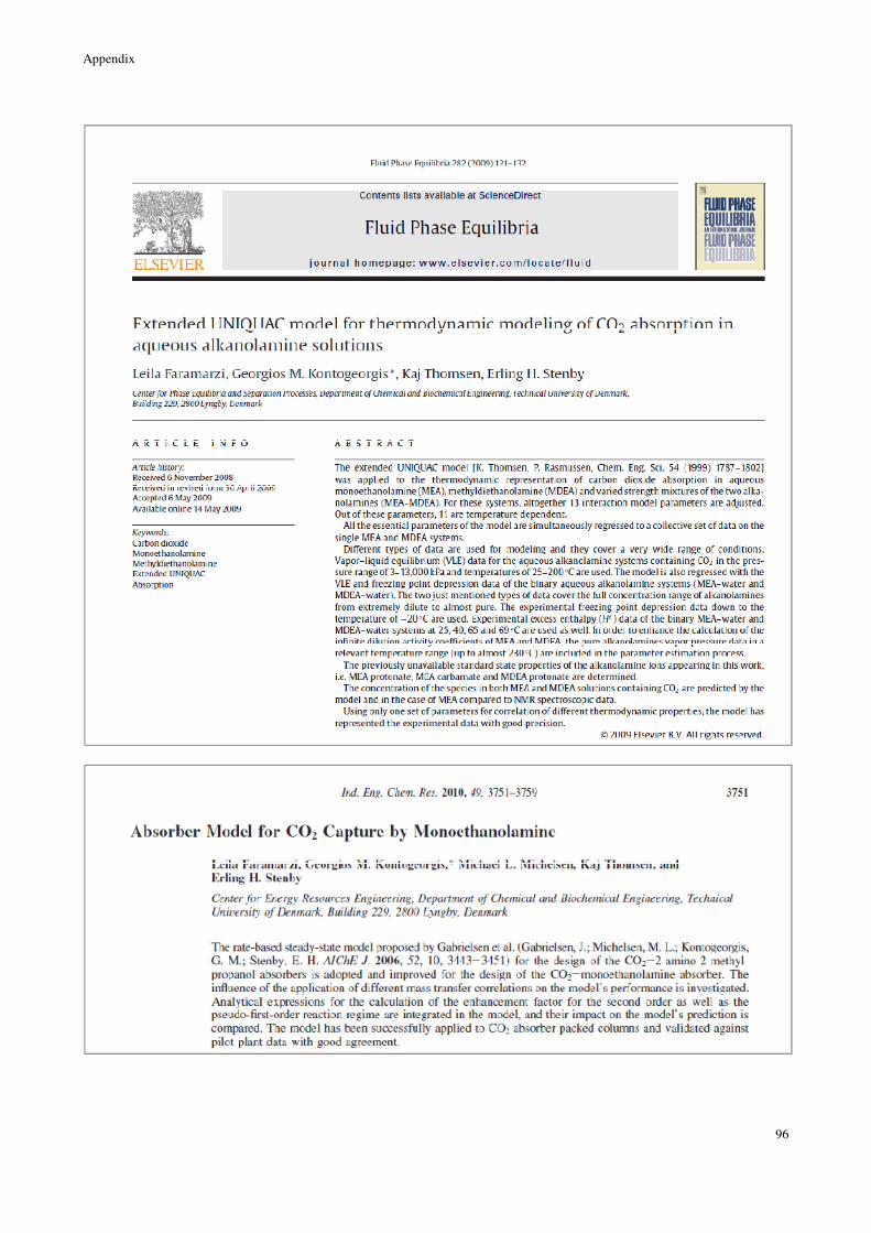
Appendix
96