Embed Size (px)
Citation preview
Possible excitation of the Possible excitation of the Chandler wobble by the Chandler wobble by the
geophysical annual cyclegeophysical annual cycle
Kosek Wiesław
Space Research Centre, Polish Academy of Sciences
Seminar at the U.S. Naval Observatory
Washington D.C. December 2003

Chandler wobble excitationChandler wobble excitation Electromagnetic torques acting on the CMB play a negligible role
in excitation of the CW (Rochester and Smylie 1965). Cumulative effect of large earthquakes was a noticeable
contribution to the CW excitation (O’Connel and Dziewonski 1976; Mansinha et al. 1979).
Seismic excitation was far too small to explain the CW excitation (Souriau and Cazenave 1985, Gross 1986).
The contribution of meteorological sources to the CW excitation was estimated as 11-19 % by Ooe (1978).
The 14.7 month signal found in the surface air pressure calculated in a coupled ocean-atmosphere general circulation model was identified as the “atmospheric pole tide” CW, so the changes in atmospheric mass distribution excite and maintain the CW and neither earthquakes nor the fluid core are significant contributions (Hameed and Currie 1989).
The joint ocean-atmosphere excitation compares substantially better with the observed excitation at the annual and Chandler frequencies than when only atmosphere is considered (Ponte et al. 1998).

Chandler wobble excitation (cont.)Chandler wobble excitation (cont.)
The importance of the OAM and AAM to the excitation of the Chandler and annual wobbles were found to be of the same order (Ponte and Stammer 1999).
The atmospheric wind and IB pressure variations maintain a major part of the observed CW, however the wind signal dominates over the IB pressure term in the vicinity of the Chandler frequency (Furuya et al. 1996; Aoyama and Naito 2001).
Celaya et al. (1999) using the results of a coupled atmosphere-ocean-land climate model, concluded that some combination of atmospheric and oceanic processes have enough power to excite the CW.
Using an 11-year time series of the OAM Brzeziński and Nastula (2002) concluded that, within the limits of accuracy, the coupled system atmosphere/ocean fully explains the CW in 1985-1996.
The most important mechanism exciting the CW in 1985-1996 was ocean-bottom pressure fluctuations, which contribute about twice as much excitation power as do atmospheric pressure fluctuations (Gross 2002).
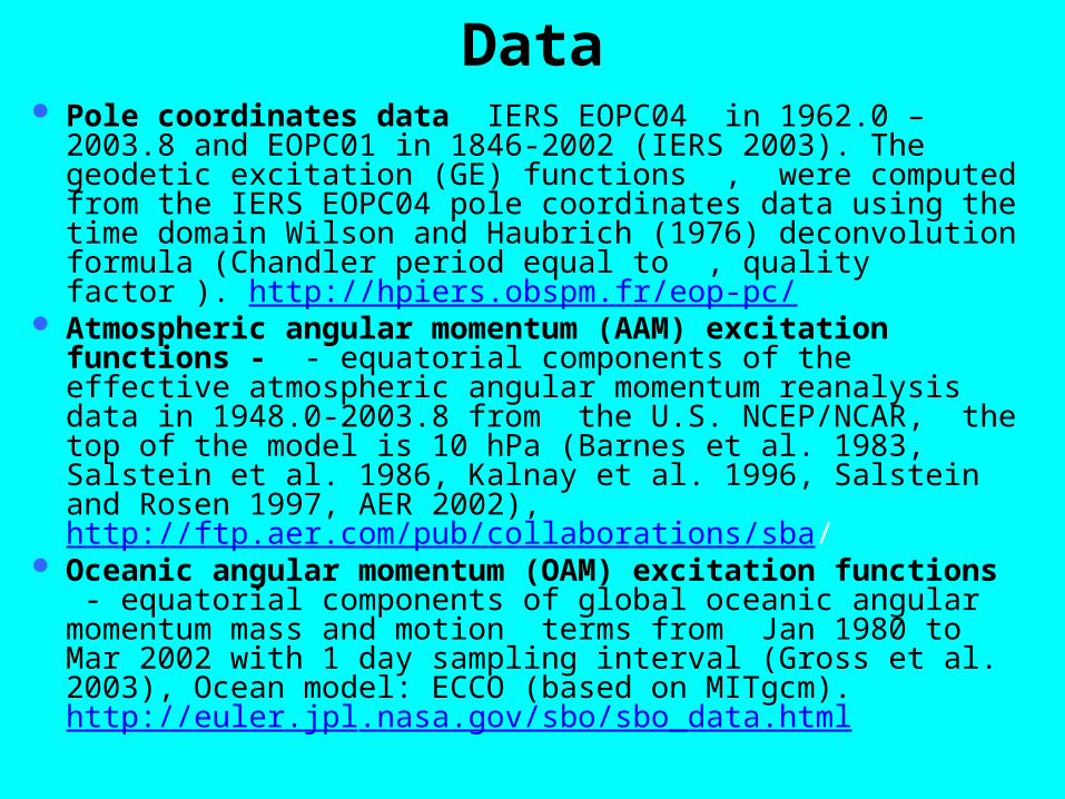
Data Pole coordinates data IERS EOPC04 in 1962.0 – 2003.8 and
EOPC01 in 1846-2002 (IERS 2003). The geodetic excitation (GE) functions , were computed from the IERS EOPC04 pole coordinates data using the time domain Wilson and Haubrich (1976) deconvolution formula (Chandler period equal to , quality factor ). http://hpiers.obspm.fr/eop-pc/
Atmospheric angular momentum (AAM) excitation functions - - equatorial components of the effective atmospheric angular momentum reanalysis data in 1948.0-2003.8 from the U.S. NCEP/NCAR, the top of the model is 10 hPa (Barnes et al. 1983, Salstein et al. 1986, Kalnay et al. 1996, Salstein and Rosen 1997, AER 2002), http://ftp.aer.com/pub/collaborations/sba/
Oceanic angular momentum (OAM) excitation functions - equatorial components of global oceanic angular momentum mass and motion terms from Jan 1980 to Mar 2002 with 1 day sampling interval (Gross et al. 2003), Ocean model: ECCO (based on MITgcm). http://euler.jpl.nasa.gov/sbo/sbo_data.html

1890 1900 1910 1920 1930 1940 1950 1960 1970 1980 1990 2000-0.50-0.40-0.30-0.20-0.100.000.100.200.300.400.50
x
arcsec
1890 1900 1910 1920 1930 1940 1950 1960 1970 1980 1990 2000-0.40-0.30-0.20-0.100.000.100.200.300.400.500.60
y
Pole coordinates data
EOPC01 EOPC04
1962

33000 36000 39000 42000 45000 48000 51000-500-400-300-200-100
0100
mas G E
1
2
33000 36000 39000 42000 45000 48000 51000-100
0100200300400500mas
AAM (w+p+ib)
AAM2
AAM1
33000 36000 39000 42000 45000 48000 51000M JD
-1000
100200300400500mas
OAM (m ass+m otion)
OAM2
OAM1
1980
1962
1948 8.2003

The mean determination error of x, y pole coordinates data
1860 1880 1900 1920 1940 1960 1980 20000.00
0.04
0.08
0.12
0.16
0.20 I ER S EOPC01 arcsec
x
y
1984 1986 1988 1990 1992 1994 1996 1998 2000 20020.0000
0.0002
0.0004
0.0006
0.0008
0.0010
0.0012
0.0014
0.0016
0.0018
0.0020
USNO
arcsec
x
y
1976 1980 1984 1988 1992 1996 20000.00
0.01
0.02
0.03
0.04
0.05
USNO
arcsec
x
y

The FTBPF amplitude spectra of complex-valued pole coordinate data in 1900-2003
-1 .8 -1.6 -1.4 -1.2 -1.0 -0.8 -0.6 -0.4 -0.2 0.0 0.2 0.4 0.6 0.8 1.0 1.2 1.4 1.6 1.8period (years)
0
40
80
120
160m as x - i y

The most energetic oscillations of polar motion computed by the FTBPFThe most energetic oscillations of polar motion computed by the FTBPF
1890 1900 1910 1920 1930 1940 1950 1960 1970 1980 1990 2000-0.30-0.20-0.100.000.100.200.30
Ch x
arcsec
1890 1900 1910 1920 1930 1940 1950 1960 1970 1980 1990 2000-0.30-0.20-0.100.000.100.200.30
Ch y
1890 1900 1910 1920 1930 1940 1950 1960 1970 1980 1990 2000-0.20-0.100.000.100.20
An x
1890 1900 1910 1920 1930 1940 1950 1960 1970 1980 1990 2000-0.20-0.100.000.100.20
An y
Chandler
Annual

The amplitude and phase variations of the Chandler and annual oscillations The amplitude and phase variations of the Chandler and annual oscillations computed by the LS in 3 year time intervals, the Nicomputed by the LS in 3 year time intervals, the Niñño indiceso indices
1977 1980 1983 1986 1989 1992 1995 1998 20010.05
0.10
0.15
0.20
0.25arcsec
am plitudes
Ch x/ yAn xAn y
1977 1980 1983 1986 1989 1992 1995 1998 2001-2
0
2
4
oC Nino 1+2 Nino 3 Nino 4
1977 1980 1983 1986 1989 1992 1995 1998 2001150
200
250
300
350o
phases
Ch x/ yAn y
An x

The amplitude of the Chandler oscillation and its first difference computed from
the x – i y data by the FTBPF and by the LS method in 5 year time intervals
1900 1910 1920 1930 1940 1950 1960 1970 1980 1990 20000.00
0.05
0.10
0.15
0.20
0.25
0.30
FTBPF
LS
arcsecChandler amplitude
1900 1910 1920 1930 1940 1950 1960 1970 1980 1990 2000-0.2
-0.1
0.0
0.1
0.2FTBPFLS
m as/day

Transformation of x, y pole coordinates data to polar coordinate systemTransformation of x, y pole coordinates data to polar coordinate system
ntt
kkAtL ,...,3,2,
2
ty
tx ,
tR
ntmtyty
mtxtxtR ,...,2,1,
22
nttytytxtxtA ,...,3,2,2
12
1
radius
angular velocity
length of polar motion path
mty
mtx ,
tA
1,
1 ty
tx
mean pole
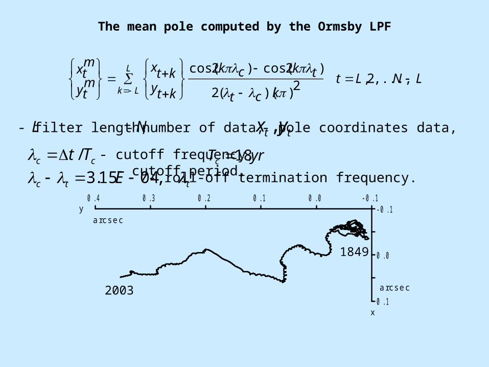
The mean pole computed by the Ormsby LPF
LNLtkct
tkck
ktyktx
mty
mtx L
Lk
,...,2,2))((2
)2cos()2cos(
L N- filter length, - number of data,
cc Tt / - cutoff frequency, - cutoff period, yrTc 18,0415.3 Etc - roll-off termination frequency.
tt yx , - pole coordinates data,
t-0.10.00.10.20.30.4
-0.1
0.0
0.1x
yarcsec
arcsec
1849
2003

1900 1910 1920 1930 1940 1950 1960 1970 1980 1990 20000.0
0.1
0.2
0.3
0.4Radiusarcsec
1900 1910 1920 1930 1940 1950 1960 1970 1980 1990 20000.000
0.002
0.004
0.006
0.008Angular velocityarcsec/day
Corr. Coeff.
1900-20030.864
1950-20030.899

The time-frequency coherence between the radius and angular velocity computed using the Morlet Wavelet Transform
2
4
6
8yrM W T coherence R , A
1
3
5
7
1910 1920 1930 1940 1950 1960 1970 1980 1990years
500
1000
1500
2000
2500
3000
perio
d (d
ays)
0 .1
0 .2
0 .3
0 .4
0 .5
0 .6
0 .7
0 .8
0 .9
red noise coherence
0 500 1000 1500 2000 2500 3000period (days)
0 . 00 . 20 . 40 . 60 . 81 . 0

The FTBPF time-frequency amplitude spectra of polar motion radius and angular velocity
1920 1930 1940 1950 1960 1970 1980years
500
1500
2500
3500
per
iod
(day
s)
0.2
0.4
0.6
0.8
1.0
1 9 20 19 3 0 1 9 4 0 1 95 0 1 9 6 0 1 9 70 1 9 8 0
500
1500
2500
3500
1 02 03 04 05 06 0
3
6
9
yr m asrad ius
angular ve locity m as/day
3
6
9
0.0001

The length of polar motion path and the envelope of the Chandler oscillationThe length of polar motion path and the envelope of the Chandler oscillation
1900 1910 1920 1930 1940 1950 1960 1970 1980 1990 2000years
-600-400-200
0200400
arcsec sum of the Chandler envelope - linear trendS
t
t
kkt ES
1
~
t
kkt AL
1
~
trendLL tt ~
trendSS tt ~
1900 1910 1920 1930 1940 1950 1960 1970 1980 1990 2000-0.3-0.2-0.10.00.10.20.3
arcsec Chandler
xy
E t
1900 1910 1920 1930 1940 1950 1960 1970 1980 1990 2000-6.0-4.0-2.00.02.0
arcsec length of polar m otion path - linear trendL
t
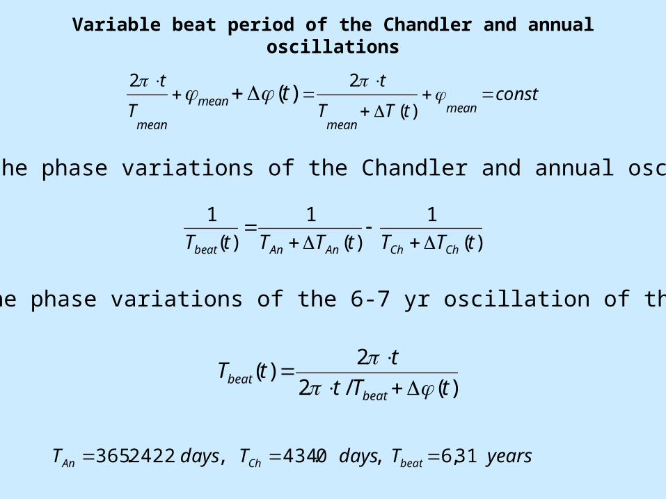
Variable beat period of the Chandler and annual oscillations
consttTT
t
T
t
meanmean
mean
mean
t
)(
22)(
)(/2
2)(
tTt
ttT
beatbeat
)(
1
)(
1
)(
1
tTTtTTtT ChChAnAnbeat
- from the phase variations of the Chandler and annual oscillations
- from the phase variations of the 6-7 yr oscillation of the radius
yearsTdaysTdaysT beatChAn 31,6,0.434,2422.365

Beat period variations computed from the LS phase variations of the Chandler and annual oscillations
1977 1980 1983 1986 1989 1992 1995 1998 2001
200
250
300
350 phasesCh x/yAn y
An x
5 yearso
1977 1980 1983 1986 1989 1992 1995 1998 2001
340360380400420440
periods
Ch x/y
An yAn x
days
1977 1980 1983 1986 1989 1992 1995 1998 200145678
years beat period
1977 1980 1983 1986 1989 1992 1995 1998 2001-2
0
2
4
oC Nino 1+2 Nino 3 Nino 4

Beat period estimated from the phase variations of the 6-7 yr oscillation of the radius.The LS amplitudes and phases computed in 12, 13 year time intervals
1950 1960 1970 1980 1990 20005.86.06.26.46.66.8 Period of 6-7yr oscillation computed from the LS phase
years
1950 1960 1970 1980 1990 20000.04
0.08
0.12
0.16 LS amplitude of 6-7yr oscillation arcsec
1950 1960 1970 1980 1990 2000210220230240250260270280 LS phase of 6-7yr oscillation
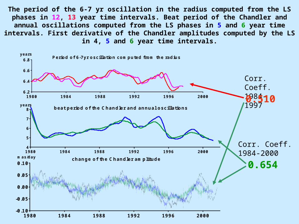
The period of the 6-7 yr oscillation in the radius computed from the LS phases in 12, 13 year time intervals. Beat period of the Chandler and annual oscillations computed from the LS
phases in 5 and 6 year time intervals. First derivative of the Chandler amplitudes computed by the LS in 4, 5 and 6 year time intervals.
1980 1984 1988 1992 1996 20006.2
6.4
6.6
6.8 Period of 6-7yr oscillation com puted from the radius years
0.654
Corr. Coeff.1984-2000
Corr. Coeff.1984-1997
0.510
1980 1984 1988 1992 1996 20004
5
6
7
8years
beat period of the Chandler and annual oscillations
1980 1984 1988 1992 1996 2000-0.10
-0.05
0.00
0.05
0.10mas/day change of the Chandler amplitude

2E+003 2E+003 2E+003 2E+003 2E+003 2E+003
100
300
500
0.1
0.2
0.3
0.4
0.5
0.6
0.7
0.8
0.9
1970 1975 1980 1985 1990 1995-600
-400
-200
2E+003 2E+003 2E+003 2E+003 2E+003 2E+003
100
300
500
p
eri
od
(d
ay
s)
1970 1975 1980 1985 1990 1995-600
-400
-200
GE & AAM
GE & (AAM + OAM)GE & AAM
The Morlet Wavelet Transform spectro-temporal coherences between the complex-valued geodetic (GE) and the atmospheric (AAM) as well as the sum of the atmospheric and oceanic (AAM+OAM) excitation functions.

The LS amplitude variations of the annual oscillation computed in four-year time intervals from the geodetic GE, atmospheric AAM and the sum of atmospheric and oceanic AAM+OAM excitation functions.
1980 1984 1988 1992 1996 2000 20040
10
20
AAM + OAM
AAMGE
mas
1 9 8 0 1 9 8 4 1 9 8 8 1 9 9 2 1 9 9 6 2 0 0 0 2 0 0 41 0
2 0
3 0
4 0
5 0
6 0
7 0
A A M + O A MA A M
G E
m a s
1980 1984 1988 1992 1996 2000 2004100
150
200
250
300
GE
AAM
AAM + OAM
o
1980 1984 1988 1992 1996 2000 2004200
250
300GE
AAMAAM + OAM
o
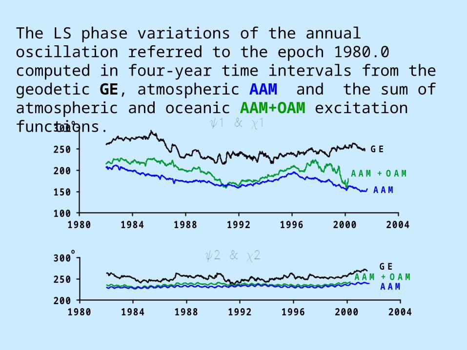
The LS phase variations of the annual oscillation referred to the epoch 1980.0 computed in four-year time intervals from the geodetic GE, atmospheric AAM and the sum of atmospheric and oceanic AAM+OAM excitation functions.

The LS phase variations of the annual oscillation computed in 3 and 4 year time intervals of the AAM+OAM excitation functions. The change of the Chandler amplitude computed by the LS in
4, 5 and 6 year time intervals.
1980 1984 1988 1992 1996 2000-0.10
-0.05
0.00
0.05
0.10mas/day change of the Chandler amplitude
Corr.coef.1984-2000
-0.592
-0.524
1980 1984 1988 1992 1996 2000150
200
250 AAM + OAMo
43
1980 1984 1988 1992 1996 2000290
300
310 AAM + OAM (retrograde)
34
o

The phase of the annual oscillation in the AAM+OAM excitation functions
decreases
The phase of the annual oscillation in polar motion
decreases
The period of the annual oscillation in polar motion
increases
The beat period of the Chandler and annual oscillations
increases
The change of the Chandler amplitude increases
The excitation mechanism of the Chandler wobble
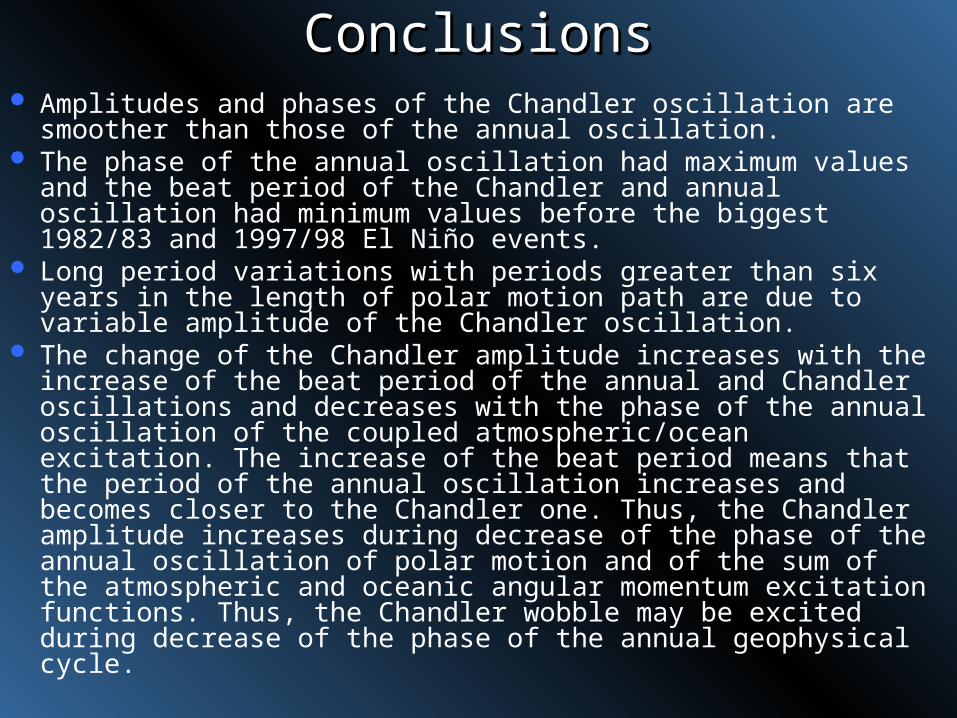
ConclusionsConclusions Amplitudes and phases of the Chandler oscillation are smoother than
those of the annual oscillation. The phase of the annual oscillation had maximum values and the
beat period of the Chandler and annual oscillation had minimum values before the biggest 1982/83 and 1997/98 El Niño events.
Long period variations with periods greater than six years in the length of polar motion path are due to variable amplitude of the Chandler oscillation.
The change of the Chandler amplitude increases with the increase of the beat period of the annual and Chandler oscillations and decreases with the phase of the annual oscillation of the coupled atmospheric/ocean excitation. The increase of the beat period means that the period of the annual oscillation increases and becomes closer to the Chandler one. Thus, the Chandler amplitude increases during decrease of the phase of the annual oscillation of polar motion and of the sum of the atmospheric and oceanic angular momentum excitation functions. Thus, the Chandler wobble may be excited during decrease of the phase of the annual geophysical cycle.

ABSTRACTIt was found that the change of the Chandler oscillation amplitude is similar to the change of the beat period of the Chandler and annual oscillations and to the negative change of the phase of the annual oscillation of the coupled atmospheric/ocean excitation. The beat period increases due to decrease of the phase of the annual oscillation, which means that the annual oscillation period increases and becomes closer to the Chandler one. The exchange of the atmospheric angular momentum and ocean angular momentum with each other and with the solid earth at the frequency equal approximately to 1 cycle per year represents the ‘geophysical annul cycle’ which can be expressed by the annual oscillation in the sum of the atmospheric and oceanic angular momentum excitation functions. The phase variations of this annual cycle are possibly responsible for the Chandler wobble excitation.


![Wobble 2.0 - User Guide - v1.0[1]](https://img.pdfslide.us/doc/110x75/577cc1821a28aba711933641/wobble-20-user-guide-v101.jpg)