Kyoto University, Graduate School of Economics Research Project Center Discussion Paper Series

Positive and Negative Population Growth and

Long-Run Trade Patterns: A Non-Scale Growth Model

Hiroaki Sasaki

Discussion Paper No. E-13-004

Research Project Center Graduate School of Economics

Kyoto University Yoshida-Hommachi, Sakyo-ku Kyoto City, 606-8501, Japan

October 2013

Positive and Negative Population Growth andLong-Run Trade Patterns: A Non-Scale Growth

Model∗

Hiroaki Sasaki†

Abstract

This paper builds a two-country, two-sector, non-scale growth model and investigatesthe relationship between trade patterns and the growth rate of per capita real consump-tion. We consider negative population growth as well as positive population growth.We show that, as long as the population growth rates of the two countries are differ-ent, if the country that accumulates capital stock has negative population growth, notrade patterns are sustainable in the long run. This is true irrespective of the populationgrowth rate of the other country. Moreover, we show that, if the country that accumu-lates capital stock has positive population growth, two trade patterns are sustainable inthe long run. In this case, either each country’s per capita growth is determined by thepopulation growth of the capital-accumulating country or the population growth of bothcountries, depending on which of the two trade patterns is realized.

Keywords: positive/negative population growth; trade patterns; non-scale growth model

JEL Classification: F10; F43; O11; O41

∗I am grateful to Grants-in-Aid for Scientific Research of Japan Society for the Promotion of Science(KAKENHI 25380295) for their financial support of this study.†Graduate School of Economics, Kyoto University. Yoshida-Honmachi, Sakyo-ku, Kyoto 606-8501, Japan.

E-mail: sasaki@econ.kyoto-u.ac.jp. Phone: +81-(0)75-753-3446

1

1 Introduction

This study investigates the relationships between population growth, trade patterns, and percapita consumption growth. We consider negative population growth as well as positivepopulation growth. For this purpose, we present a two-country, two-sector, two-factor, non-scale growth model.

In scale-growth models, the long-run growth rate of per capita income is proportionalto the scale of the population, which seems counterfactual. On the other hand, in non-scale growth models, the long-run growth rate of per capita income is proportional to thegrowth rate of the population. A pioneering work on non-scale growth models was thatof Jones (1995). Jones (1995) attempted to remove the scale effects, and presented a non-scale growth model in which the growth rate of output per capita depends positively onthe population growth rate, and not on the size of the population. That is, the higher thepopulation growth rate, the faster the country grows.1)

We use the non-scale growth model for two reasons. First, we can obtain sustainableincome per capita growth, even when population growth is strictly positive. Second, we donot need to impose knife-edge conditions on the parameters of the model.

Other studies analyze the relationship between trade patterns and growth.2) Two goodexamples are the studies by Kaneko (2003) and Felbermayr (2007).

Kaneko (2003) builds a two-country, two-sector, AK growth model and endogenizes theterms of trade.3) He finds that, if an autarkic country with a lower growth rate than its tradepartner has a comparative advantage in the consumption goods sector, then the country cannarrow or even reverse the growth gap by opening trade.

Felbermayr (2007) describes a situation in which a capital-abundant North and a capital-scarce South trade with each other. In his model, the trade pattern is endogenously deter-mined, and he analyzes the situation in which the North produces investment goods and theSouth produces consumption goods. The production technology of investment goods is AKand that of consumption goods is decreasing returns to scale. Along the balanced growthpath, the Southern terms of trade are continuously improving such that, even with the de-

1) For a systematic exposition of scale effects and non-scale growth, see Jones (1999), Jones (2005), Aghionand Howitt (2005), and Dinopoulos and Sener (2007). For more sophisticated non-scale growth models, seealso Kortum (1997), Dinopoulos and Thompson (1998), Peretto (1998), Segerstrom (1998), Young (1998),Howitt (1999), and Dinopoulos and Syropoulos (2007).

2) Wong and Yip (1999) present a small, open-economy, two-sector model of endogenous growth, includ-ing capital accumulation and learning by doing. They analyze the relationship between economic growth,industrialization, and international trade.

3) Kaneko (2000) builds a growth model with human capital accumulation and shows that the relationshipbetween the terms of trade and growth depends on whether the country specializes in the consumption goodssector or the investment goods sector. However, Kaneko’s (2000) model is a small, open-economy model,which means the terms of trade are exogenous.

2

creasing returns to scale, the South can grow at the same rate as the North. Therefore, theSouth can eliminate the growth gap by opening trade.

However, these are both scale growth models, and hence are subject to the aforemen-tioned problems specific to these models.

In contrast, examples of studies that investigate the relationship between trade patternsand growth rates using non-scale growth models include Sasaki (2011a) and Sasaki (2012).Sasaki (2011a) derives a model to investigate which trade pattern is realized in the long runwhen both countries’ population growth rates are equal. Then, Sasaki (2012) extends thismodel to include the case in which the countries’ population growth rates are different.4)

However, both studies consider only positive population growth. Accordingly, we considercases in which population growth is both negative and positive.

Many developed countries have stagnant population growth, and in some cases, a neg-ative growth rate.5) Existing economic growth theories assume positive population growth.However, given that population growth can be negative, we need to consider this case aswell.

At first, it may seem easy to include negative population growth in economic growth the-ory, but this is not the case.6) As Ferrara (2011) and Christiaans (2011) show, incorporatingnegative population growth in growth models is more complicated than simply replacing apositive value with a negative value.

Christiaans (2011) shows the importance of negative population growth using a simplemodel. Consider a Solow growth model with a production function that exhibits increasing,but relatively small returns to scale.7) When the population growth rate is positive, per capitaincome growth is positive and increasing in the population growth rate. On the other hand,when the population growth rate is negative, contrary to expectations, per capita incomegrowth remains positive, but is decreasing in the population growth rate.

Using a two-country model of international trade, we investigate the relationships be-tween the size of exogenously given population growth rates, the sustainability of tradepatterns, and the long-run growth rate of per capita consumption in each country, given that

4) In this respect, Sasaki (2011b) builds a non-scale growth, North-South economic development model,and shows that both countries grow at the same rate along the balanced growth path. However, their percapita incomes grow at different rates because the differences in population growth. Nevertheless, since theproduction pattern is fixed and given exogenously in this model, we cannot know whether the given tradepattern is sustainable over time.

5) For example, according to Japan’s Ministry of Internal Affairs and Communications, as of March 2012,Japan has experienced its largest-ever decline in population.

6) Ritschel (1985) argues that, in the standard Solow growth model, a negative savings rate is necessary forthe existence of a steady-state equilibrium with a negative population growth rate. See also Felderer (1988).

7) In the Solow model with a constant returns to scale production function, per capita income growth is zerowhen the population growth is positive, but positive when the population growth is negative. For details, seeChristiaans (2011).

3

a specific trade pattern is sustainable.The main results are as follows. We show that, as long as the population growth rates

of the two countries are different, if the country that accumulates capital stock has nega-tive population growth, no trade patterns are sustainable in the long run, irrespective of thepopulation growth rate of the other country. Moreover, we show that, if the country that ac-cumulates capital stock has positive population growth, two trade patterns are sustainable inthe long run. Here, either each country’s growth rate is determined by the population growthof the capital-accumulating country or the population growth of both countries, dependingon which of the two trade patterns is realized.

The rest of the paper is organized as follows. Section 2 presents our model and deter-mines the equilibrium and long-run growth rate of per capita consumption under autarky.Section 3 investigates the equilibrium under free trade. Section 4 investigates the long-rungrowth rate of per capita consumption under free trade. We compare the growth rates underfree trade and autarky, and then compare our results to those of related studies. Finally,Section 5 concludes the paper.

2 The model

Consider a world that contains two countries: Home and Foreign. Both countries producehomogeneous manufactured and agricultural goods. The manufactured good is used for bothconsumption and investment, whereas the agricultural good is used only for consumption.

2.1 Production

Firms produce manufactured goods, XMi , with labor input, LM

i , and capital stock, Ki, andproduce agricultural goods, XA

i , with only labor input, LAi . Here, i = 1 and i = 2 denote

Home and Foreign, respectively. Both countries have the same production functions, whichare specified as follows:

XMi = AiKαi (LM

i )1−α, where Ai = Kβi (1)

= Kα+βi (LMi )1−α, 0 < α < 1, 0 < β < 1, α + β < 1, (2)

XAi = LA

i . (3)

Here, Ai in equation (1) represents an externality associated with capital accumulation,which captures the learning-by-doing effect introduced by Arrow (1962). Substituting Ai

into equation (1), we obtain equation (2), which shows that manufactured goods production

4

has increasing returns to scale, with β corresponding to the extent of the increasing returns.Equation (3) shows that agricultural goods production has constant returns to scale.

We further suppose that the labor supply is equal to the population and that the popula-tion is fully employed. Moreover, the population grows at a constant rate, ni, and the initialpopulation is unity in each country: Li(t) = LM

i (t)+ LAi (t) = enit, ni ≷ 0. Note that population

growth can be negative.Let pi denote the price of manufactured goods relative to agricultural goods. Then, the

profits of the manufacturing and agricultural firms are given by πMi = piXM

i − wiLMi − piriKi

and πAi = XA

i − wiLAi , respectively, where wi denotes the wage paid to produce agricultural

goods and ri denotes the rental rate of capital.From the profit-maximizing conditions, we obtain the following relations:

pi∂XM

i

∂LMi

= wi = 1, (4)

∂XMi

∂Ki= ri with Ai given. (5)

From equation (4), we find that the wage is unity as long as agricultural production is posi-tive. We assume a Marshallian externality in deriving equation (5); profit-maximizing firmsregard Ai as exogenously given. Accordingly, firms do not internalize the effect of Ai.

2.2 Consumption

For simplification, we make the classical assumption that wage income and capital incomeare entirely devoted to consumption and saving, respectively.8) In the canonical one-sectorSolow model, under the golden rule steady state in which per capita consumption is max-imized, consumption is equal to the total real wage and total capital income is saved andinvested. Hence, our assumption has some rationality and can be interpreted as a simple ruleof thumb for consumers with dynamic optimization (Christiaans, 2008). We define real con-sumption per capita, ci, as ci = Ci/Li = (CM

i )γ(CAi )1−γ/Li, where Ci denotes economy-wide

real consumption. In this case, a fraction, γ, of wage income is spent on CMi and the rest,

8) The same assumption is used in Uzawa (1961), which considers a two-sector growth model, and Krugman(1981), which considers a two-country, two-sector, North-South trade and development model. If dynamicoptimization is used, then the Euler equation for consumption appears and the number of differential equationsincreases, significantly complicating the analysis. Therefore, an analysis with dynamic optimization will be leftfor future research. In addition, it is true that consumption smoothing with dynamic optimization is a standardtool in macroeconomics, although Mankiw (2000) states that, in reality, consumption behavior deviates fromconsumption smoothing.

5

1 − γ, is spent on CAi .

piCMi = γwiLi, (6)

CAi = (1 − γ)wiLi. (7)

Moreover, the following relationship between real investment, Ii, and saving holds: piIi =

piriKi. From this equation, we obtain the rate of capital accumulation:

gKi ≡Ki

Ki= ri. (8)

That is, the rate of capital accumulation is equal to the rental rate of capital. A dot over avariable denotes the time derivative of the variable (e.g., Ki ≡ dKi/dt).

2.3 Equilibrium under autarky and per capita consumption growth

Under autarky, both goods have to be produced. The market-clearing conditions are as fol-lows: XM

i = CMi + Ii and XA

i = CAi . Note that wi = 1 under autarky. From the market-clearing

condition for manufactured goods, we obtain pi, which is used to derive each sector’s em-ployment share: LM

i /Li = γ and LAi /Li = 1 − γ. Therefore, under autarky, each sector’s

employment share is constant.Under autarky, the relative price of manufactured goods is given by

pi =(γLi)α

(1 − α)Kα+βi

. (9)

First, we derive the balanced-growth path (BGP) under autarky when the populationgrowth rate is positive, that is, ni > 0. Along the BGP, the rate of capital accumulationis constant and equal to the rental rate of capital, which is given in equation (5) as ri =

αKα+β−1i (γLi)1−α. With gKi/gKi = (α + β − 1)gKi + (1 − α)ni = 0, the BGP growth rates of Ki

and pi are, respectively, given by

g∗Ki=

1 − α1 − α − β ni > 0, (10)

g∗pi= − β

1 − α − β ni < 0, (11)

where gx ≡ x/x denotes the growth rate of a variable x and an asterisk “∗” denotes a BGPvalue. The rate of capital accumulation is positive and proportionate to population growth,and the relative price of manufactured goods is decreasing at a constant rate.

6

Consumption is defined as wages only, and hence, the growth rate of per capita realconsumption is equal to the growth rate of the real wage.9)

gci = gwi − γgpi . (12)

Here, the real wage is deflated by the consumer price index, pγi .10) To obtain gci , we mustknow gwi and gpi . Note that, as long as agricultural goods are produced, the nominal wage isequal to unity, that is, wi = 1, which means that gwi = 0. Accordingly, we obtain the growthrate of per capita consumption under autarky as follows:

gATci=

γβ

1 − α − β ni > 0, (13)

where “AT” denotes autarky. Therefore, gATci

is increasing in ni.Considering the BGP growth rate of capital stock, we introduce a new variable, scale-

adjusted capital stock: ki ≡ Ki/Lϕi , where ϕ ≡ 1−α

1−α−β . The dynamics of the scale-adjustedcapital stock are given by

ki = αγ1−αkα+βi − ϕniki. (14)

In the steady state, ki = 0, from which we obtain

k∗i =(αγ1−α

ϕni

) 11−α−β

. (15)

The steady state is stable because dki/ki|ki=k∗i = −k∗i [(1 − α − β)αγ1−α(k∗i )α+β−2 + ϕni] < 0.Next, we derive the long-run equilibrium under autarky when the population growth rate

is negative, that is, ni < 0. If ni < 0, from equation (14), there never exists a ki > 0 suchthat ki = 0, and we have ki > 0 for ki > 0. That is, if the initial value of the capital stock isstrictly greater than zero, ki(0) > 0, then ki diverges to infinity. However, even in this case,we can examine the long-run growth rate of per capita consumption. Considering that percapita consumption is equal to the real wage measured in terms of the consumer price index,

9) In every case in our model, the long-run growth rate of per capita real consumption is equal to that of percapita real income. Therefore, we use the growth rate of per capita real consumption.10) Let pc denote the consumer price index that is consistent with the expenditure minimization problem ofconsumers. Then, pc = γ

−γ(1 − γ)−(1−γ) pγi , and by definition, pcci = wi. Strictly speaking, the consumer priceindex is given by γ−γ(1 − γ)−(1−γ) pγi . However, we use pγi because the constant terms have no effect on theresults.

7

we have

gATci= −γgpi = −γ[αni − (α + β)(gki + ϕni)]

= α(α + β)γ2−αkα+β−1i − γαni. (16)

Since α + β − 1 < 0 by assumption, kα+β−1i approaches zero when ki approaches infinity.

From this, we have

limki→+∞

gATci= −γαni > 0. (17)

Therefore, gATci

is positive, even when ni < 0 and is decreasing in ni.

3 Equilibrium under free trade

Suppose that Home and Foreign engage in free trade at time zero. If K1(0) > K2(0), thenfrom equation (9), p1(0) < p2(0) because L1(0) = L2(0) = 1. Thus, if K1(0) > K2(0),Home has a comparative advantage in manufactured goods and Foreign has a comparativeadvantage in agricultural goods. In the following analysis, we assume that K1(0) > K2(0)without loss of generality.

It is sufficient for our purpose to consider the following four trade patterns from theviewpoint of Home:

Pattern 1: Both countries produce both goods; that is, both countries diversify.Pattern 2: Home diversifies and Foreign completely specializes in agriculture.Pattern 3: Home completely specializes in manufacturing and Foreign completely special-

izes in agriculture.Pattern 4: Home completely specializes in manufacturing and Foreign diversifies.

In addition, we consider the following eight cases according to the size of the populationgrowth: Case 1, 0 < n1 = n2;11) Case 2, n1 = n2 < 0; Case 3, 0 < n2 < n1; Case 4,0 < n1 < n2; Case 5, n2 < 0 < n1; Case 6, n1 < 0 < n2; Case 7, n2 < n1 < 0; and Case 8,n1 < n2 < 0.

11) Long-run growth rates and transitional dynamics in the case where 0 < n1 = n2 are analyzed in detail inSasaki (2011a). When n1 , n2, with regard to the state variable ki, the locus of ki = 0 moves over time, whichcomplicates the analysis. The analysis of transitional dynamics, including a numerical analysis when n1 , n2,is left for future research.

8

3.1 Equilibrium when both countries diversify: Pattern 1

The market-clearing conditions for both goods are given by

XM1 + XM

2 = CM1 +CM

2 + I1 + I2, (18)

XA1 + XA

2 = CA1 +CA

2 . (19)

From these, we obtain

p =[γ(L1 + L2)]α

(1 − α)(Kα+βα

1 + Kα+βα

2

)α . (20)

Each country’s employment share of the manufacturing sector, θMi , is given by

θM1 ≡

LM1

L1=γ(1 + L2

L1

)1 +

(K2K1

) α+βα

, θM2 ≡

LM2

L2=γ(1 + L1

L2

)1 +

(K1K2

) α+βα

. (21)

The rates of capital accumulation in both countries are given by

gK1 = αKα+β−11 (θM

1 L1)1−α, gK2 = αKα+β−12 (θM

2 L2)1−α. (22)

First, if n1 = n2, so that L1 = L2,12) then, after enough time has passed, we obtain

limt→+∞θM

1 = 2γ, limt→+∞θM

2 = 0, (23)

where γ < 1/2 is needed. Then, the manufacturing employment share in Foreign goes tozero, and Foreign asymptotically completely specializes in agriculture.13) Hence, Pattern 1is not sustainable when n1 = n2.

Second, if n1 > n2, then after enough time has passed, we obtain

limt→+∞θM

1 = γ, limt→+∞θM

2 = 0. (24)

In this case too, the manufacturing employment share in Foreign goes to zero, and Foreignasymptotically completely specializes in agriculture. Hence, Pattern 1 also is unsustainable

12) In addition, if K1(0) = K2(0), the manufacturing employment share in each country is given by θMi = γ,

which is constant. Pattern 1 is only sustainable in this case. However, the relative prices in both countriesunder autarky are equal, and therefore trade does not occur.13) In our model, the agricultural output approaches zero, but it never vanishes because we assume that For-eign’s capital stock is strictly positive. Therefore, the phrase “asymptotically” completely specializes in agri-culture is more appropriate. For more information, see Christiaans (2008).

9

when n1 > n2.Third, if n1 < n2, then after enough time has passed, we obtain

limt→+∞θM

1 = +∞, limt→+∞θM

2 = 0. (25)

In this case, the manufacturing employment share in Home exceeds unity, the manufac-turing employment share in Foreign goes to zero, and Foreign asymptotically completelyspecializes in agriculture. Hence, Pattern 1 also is unsustainable when n1 < n2.

Summarizing the above results, we obtain the following proposition.

Proposition 1. Pattern 1, in which both Home and Foreign diversify, is unsustainable in thelong run in every case.

3.2 Equilibrium when Home diversifies and Foreign specializes in agri-culture: Pattern 2

The market-clearing conditions for both goods are given by

XM1 = CM

1 +CM2 + I1, (26)

XA1 + XA

2 = CA1 +CA

2 . (27)

Hence, we obtain

p =[γ(L1 + L2)]α

(1 − α)Kα+β1

. (28)

The manufacturing employment share in Home is given by

θM1 = γ

(1 +

L2

L1

). (29)

First, if n1 = n2, the manufacturing employment share in Home becomes

θM1 = 2γ. (30)

In this case, we need γ < 1/2 for Pattern 2 to hold. Second, if n1 > n2, we obtain

limt→+∞θM

1 = γ. (31)

Here, the manufacturing employment share of Home converges to γ, and thus Pattern 2 is

10

sustainable. Third, if n1 < n2, then θM1 continues to increase, becomes more than unity, and

approaches infinity.

limt→+∞θM

1 = +∞. (32)

In this case, Pattern 2 is again unsustainable.The growth rate of capital stock is given by

gK1 = αγ1−α(L1 + L2)1−αKα+β−1

1 . (33)

Note that, in this case, we obtain c1 = c2 because w1 = w2 = 1 as long as agriculturalgoods are produced and both countries face the same relative price, p. Accordingly, inPattern 2, the long-run growth rates of per capita consumption in Home and Foreign areequalized; that is, gFT

c1= gFT

c2, where “FT” denotes free trade.

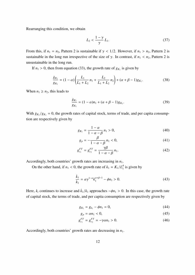
We now examine in detail the conditions under which Pattern 2 holds. Following Wongand Yip (1999), we investigate whether the trade pattern is sustainable by comparing thesize of the terms of trade and the size of the marginal rate of transformation (MRT) ofthe production possibilities frontier (PPF) at the corner point where a country completelyspecializes in manufacturing.

[Figure 1 around here]

The size of the MRT of the PPF in Home is given by

−dXA

1

dXM1

=[Kα+β1 (θM

1 L1)1−α]α

1−α

(1 − α)Kα+β1−α1

. (34)

Substituting θM1 = 1 into equation (34), the size of the MRT at the point where Home

completely specializes in manufacturing is given by

χ1 =Lα1

(1 − α)Kα+β1

. (35)

For Pattern 2 to be sustainable over time, we need p < χ1; that is, from equations (28)and (35),

[γ(L1 + L2)]α

(1 − α)Kα+β1

<Lα1

(1 − α)Kα+β1

. (36)

11

Rearranging this condition, we obtain

L2 <1 − γγ

L1. (37)

From this, if n1 = n2, Pattern 2 is sustainable if γ < 1/2. However, if n1 > n2, Pattern 2 issustainable in the long run irrespective of the size of γ. In contrast, if n1 < n2, Pattern 2 isunsustainable in the long run.

If n1 > 0, then from equation (33), the growth rate of gK1 is given by

gK1

gK1

= (1 − α)(

L1

L1 + L2n1 +

L2

L1 + L2n2

)+ (α + β − 1)gK1 . (38)

When n1 ≥ n2, this leads to

gK1

gK1

= (1 − α)n1 + (α + β − 1)gK1 . (39)

With gK1/gK1 = 0, the growth rates of capital stock, terms of trade, and per capita consump-tion are respectively given by

gK1 =1 − α

1 − α − β n1 > 0, (40)

gp = −β

1 − α − β n1 < 0, (41)

gFTc1= gFT

c2=

γβ

1 − α − β n1. (42)

Accordingly, both countries’ growth rates are increasing in n1.On the other hand, if n1 < 0, the growth rate of k1 = K1/L

ϕ1 is given by

k1

k1= αγ1−αkα+β−1

1 − ϕn1 > 0. (43)

Here, ki continues to increase and k1/k1 approaches −ϕn1 > 0. In this case, the growth rateof capital stock, the terms of trade, and per capita consumption are respectively given by

gK1 = gk1 − ϕn1 = 0, (44)

gp = αn1 < 0, (45)

gFTc1= gFT

c2= −γαn1 > 0. (46)

Accordingly, both countries’ growth rates are decreasing in n1.

12

However, we must also consider another condition to ascertain the sustainability of Pat-tern 2, that is, the relationship between the MRT of the PPF in Foreign and the terms of trade.The size of the MRT at the point where Foreign completely specializes in manufacturing isgiven by

χ2 =Lα2

(1 − α)Kα+β2

. (47)

For Pattern 2 to be sustainable in the long run, it is necessary that p < χ2.There exist five cases such that n1 ≥ n2: 0 < n1 = n2 (Case 1); n1 = n2 < 0 (Case 2);

0 < n2 < n1 (Case 3); n2 < 0 < n1 (Case 5); and n2 < n1 < 0 (Case 7).Case 1: If 0 < n1 = n2, we find that p < χ2 holds over time because, in the long run,gp = − β

1−α−β n1 < 0 and gχ2 = αn1 > 0. Therefore, Pattern 2 is sustainable.Case 2: If n1 = n2 < 0, we find that p < χ2 holds over time because, in the long run,gp = gχ2 = αn1. Therefore, Pattern 2 is sustainable.Case 3: If 0 < n2 < n1, we find that p < χ2 holds over time because gp = − β

1−α−β n1 < 0 andgχ2 = αn2 > 0. Therefore, Pattern 2 is sustainable.Case 5: If n2 < 0 < n1, we have gp = − β

1−α−β n1 < 0 and gχ2 = αn2 < 0. For the conditionp < χ2 to hold in the long run, we need |gp| > |gχ2 |.

|gp| − |gχ2 | =β

1 − α − β n1 + αn2. (48)

Accordingly, if β

1−α−β n1+αn2 > 0, Pattern 2 is sustainable. In contrast, if β

1−α−β n1+αn2 < 0,Pattern 2 is unsustainable.Case 7: If n2 < n1 < 0, we have gp = αn1 < 0 and gχ2 = αn2 < 0, which imply that

|gp| − |gχ2 | = α(n2 − n1) < 0. (49)

This contradicts |gp| > |gχ2 |, and so Pattern 2 is unsustainable.Summarizing the above results, we obtain the following propositions.

Proposition 2. Pattern 2 (Home diversifies while Foreign asymptotically completely spe-cializes in agriculture) is sustainable in the long run in Cases 1, 2, 3, and 5.

Proposition 3. If Pattern 2 is sustainable in the long run, both countries grow at the sameper capita rate under free trade, irrespective of whether their population growth is positiveor negative.

Note that Cases 1 and 2 require γ ≤ 1/2, while Case 5 requires β

1−α−β n1 + αn2 > 0.

13

The reason why this trade pattern is unsustainable in the long run when n1 < n2 is thatdemand for manufactured goods in Foreign grows faster than the supply from Home. As aresult, Home cannot meet the world demand for manufactured goods on its own.

3.3 Equilibrium when Home specializes in manufacturing and Foreignspecializes in agriculture: Pattern 3

The market-clearing conditions for both goods are given by

XM1 = CM

1 +CM2 + I1, (50)

XA2 = CA

1 +CA2 . (51)

With LM1 = L1, because of complete specialization in manufacturing, we obtain

p =γL2

(1 − α)(1 − γ)Kα+β1 L1−α1

. (52)

The growth rate of capital stock is given by

gK1 = αKα+β−11 L1−α

1 . (53)

Pattern 3 is sustainable if p > χ1, which, from equations (35) and (52), can be rewrittenas

γL2

(1 − α)(1 − γ)Kα+β1 L1−α1

>Lα1

(1 − α)Kα+β1

. (54)

From this, we obtain

L2 >1 − γγ

L1. (55)

Therefore, if n1 = n2, Pattern 3 is sustainable as long as γ > 1/2. If n2 > n1, Pattern 3is sustainable in the long run, irrespective of the size of γ. On the other hand, if n2 < n1,Pattern 3 is unsustainable in the long run. In summary, n2 ≥ n1 is necessary for Pattern 3 tobe sustainable.

Note that, in this case, we obtain c1 > c2 because w1 = [γ/(1−γ)] · (L2/L1) > 1 > w2 = 1when n2 > n1, and both countries face the same relative price, p.

If n1 > 0, the growth rates of the capital stock, terms of trade, and per capita consumption

14

are given by

gK1 =1 − α

1 − α − β n1 > 0, (56)

gp = n2 −1 − α

1 − α − β n1, (57)

gFTc1= (n2 − n1) − γ

(n2 −

1 − α1 − α − β n1

)=β − (1 − γ)(1 − α)

1 − α − β n1 + (1 − γ)n2, (58)

gFTc2=γ(1 − α)1 − α − β n1 − γn2. (59)

Accordingly, gFTc1

is increasing in n1 if β > (1−γ)(1−α), decreasing in n1 if β < (1−γ)(1−α),and increasing in n2. In addition, gFT

c2is increasing in n1 and decreasing in n2. In standard

non-scale growth models, the growth rate of per capita consumption (income) is increasingin the growth rate of population. However, in our model, Home’s per capita consumptiongrowth can be increasing or decreasing in its population growth, and Foreign’s per capitaconsumption growth is decreasing in its population growth.14)

On the other hand, if n1 < 0, the growth rate of k1 is given by

k1

k1= αkα+β−1

1 − ϕn1 > 0. (60)

Accordingly, k1 continues to increase over time. When k1 increases, k1/k1 approaches−ϕn1 > 0. From this, we obtain

gK1 = 0, (61)

gp = n2 − (1 − α)n1, (62)

gFTc1= (n2 − n1) − γ[n2 − (1 − α)n1] = −[1 − γ(1 − α)]n1 + (1 − γ)n2, (63)

gFTc2= −γ[n2 − (1 − α)n1] = γ(1 − α)n1 − γn2. (64)

Accordingly, gFTc1

is decreasing in n1 and increasing in n2. In addition, gFTc2

is increasing inn1 and decreasing in n2.

However, as in Pattern 2, we must also consider another condition. For Pattern 3 to besustainable in the long run, we need p < χ2.

There exist five cases such that n1 ≤ n2: 0 < n1 = n2 (Case 1); n1 = n2 < 0 (Case 2);0 < n1 < n2 (Case 4); n1 < 0 < n2 (Case 6); and n1 < n2 < 0 (Case 8).

14) Sasaki (2011b) presents empirical evidence indicating that, in developed countries, the correlation betweenper capita income growth and population growth is ambiguous, whereas in developing countries, the correlationis negative.

15

Case 1: If 0 < n1 = n2, we obtain gp = − β

1−α−β n1 < 0 and gχ2 = αn1 > 0, which show thatp < χ2 holds over time, and hence, Pattern 3 is sustainable.Case 2: If n1 = n2 < 0, we obtain gp = αn1 < 0 and gχ2 = αn1 < 0, which show that p < χ2

holds over time, and hence, Pattern 3 is sustainable.Case 4: If 0 < n1 < n2, we have gp = n2 − 1−α

1−α−β n1 and gχ2 = αn2 > 0. In this case, weobtain

|gχ2 | − |gp| = −(1 − α)(n2 −

11 − α − β n1

). (65)

If n2 <1−α

1−α−β n1, that is, gp < 0, Pattern 3 is sustainable. If n2 >1−α

1−α−β n1, that is, gp > 0, weneed n2 <

11−α−β n1 for |gχ2 | > |gp| to hold. Therefore, if 1−α

1−α−β n1 < n2 <1

1−α−β n1, Pattern 3 issustainable. On the other hand, if 1

1−α−β n1 < n2, Pattern 3 is unsustainable. In summary, ifn2 <

11−α−β n1, Pattern 3 is sustainable.

Case 6: If n1 < 0 < n2, we have gp = n2 − (1 − α)n1 > 0 and gχ2 = αn2 > 0. For Pattern 3 tobe sustainable, we need |gχ2 | > |gp|. However, we obtain

|gχ2 | − |gp| = −(1 − α)(n2 − n1) < 0. (66)

Accordingly, Patterns 3 is unsustainable in this case.Case 8: If n1 < n2 < 0, we have gp = n2− (1−α)n1 and gχ2 = αn2 < 0. If n2− (1−α)n1 > 0,that is, gp > 0, Pattern 3 is clearly unsustainable. If n2 − (1 − α)n1 < 0, that is, gp < 0, weneed |gp| > |gχ2 | for Pattern 3 to be sustainable. However, we obtain

|gp| − |gχ2 | = −(1 − α)(n2 − n1) < 0. (67)

Therefore, Pattern 3 is unsustainable in this case.Summarizing the above results, we obtain the following propositions.

Proposition 4. Pattern 3 (Home completely specializes in manufacturing while Foreignasymptotically completely specializes in agriculture) is sustainable in the long run in Cases1, 2, and 4.

Proposition 5. If Pattern 3 is sustainable in the long run and if both countries’ populationgrowth rates are different, both countries grow at different per capita rates under free trade.

Note that Cases 1 and 2 require 1/2 < γ, while Case 4 requires n2 <1

1−α−β n1.The reason why this trade pattern is unsustainable in the long run when n1 > n2 is that

demand for agricultural goods in Home grows faster than they are supplied by Foreign.Hence, Foreign cannot meet the world demand for agricultural goods on its own.

16

3.4 Equilibrium when Home specializes in manufacturing and Foreigndiversifies: Pattern 4

The market-clearing conditions for both goods are given by

XM1 + XM

2 = CM1 +CM

2 + I1 + I2, (68)

XA2 = CA

1 +CA2 . (69)

From equations (68) and (69), we find that the terms of trade satisfy the following equation:

(1 − α)1α p

1αK

α+βα

2 = γL2 − (1 − α)(1 − γ)pKα+β1 L1−α1 . (70)

Here, p is implicitly and uniquely determined from equation (70), and hence, p is a functionof K1, K2, L1, and L2: p = p(K1,K2, L1, L2).15)

The growth rate of the capital stock in each country is given by

gK1 = αKα+β−11 L1−α

1 , gK2 = α(1 − α)1−αα p

1−αα K

βα

2 , (71)

where p is endogenously determined by equation (70).The employment share of manufacturing in Foreign is given by

θM2 =

(1 − α)1α p

1αK

α+βα

2

L2. (72)

In this case, analytical solutions are difficult to obtain, so we conduct numerical simula-tions.16) Using equation (70), we obtain the time derivative of p as follows:

p =γL2 − (1 − α)2(1 − γ)pKα+β1 L−α1 L1 − (1 − α)(1 − γ)(α + β)pKα+β−1

1 L1−α1 K1 − α+βα (1 − α)

1αK

βα

2 K2

1α(1 − α)

1α p

1−αα K

α+βα

2 + (1 − α)(1 − γ)Kα+β1 L1−α1

.

(73)

Substituting L1 = n1L1, L2 = n2L2, and the two equations from (71) into equation (73), weobtain the differential equation of p.

Using the initial conditions K1(0), K2(0), L1(0), L2(0), as well as the parameters, we can

15) The left-hand side of equation (70) is an increasing function of p, whereas the right-hand side of thisequation is a decreasing function of p for given values of K1, K2, L1, and L2. Plotting both functions, we findthat their intersection is unique and gives an instantaneous equilibrium value of p.16) We use the following values for the parameters and initial capital stocks: α = 0.3, β = 0.2, γ = 0.6,K1(0) = 1.2, K2(0) = 1.

17

obtain the initial value of the terms of trade, p(0), using equation (70). Using this initialvalue, p(0), and equation (73), we obtain the time path of p(t).

From the numerical simulation, we find that, regardless of whether n1 ⋛ n2, the manufac-turing employment share in Foreign tends to zero in finite time; that is, θM

2 → 0. Therefore,Pattern 4 is unsustainable in the long run.

Proposition 6. Pattern 4 (Home completely specializes in manufacturing while Foreign di-versifies) is unsustainable in the long run in every case.

4 Per capita consumption growth under free trade

From the above analysis, we find that the sustainable trade patterns are Patterns 2 and 3. Inthis section, we summarize the long-run growth rate of per capita consumption under freetrade according to the rate of the population growth.

4.1 Case 1: 0 < n1 = n2

If 0 < γ < 1/2, only Pattern 2 is sustainable, and if 1/2 < γ < 1, only Pattern 3 is sustainable.In both cases, the BGP growth rates of per capita consumption are given by

gFTc1= gFT

c2=

γβ

1 − α − β n1 > 0. (74)

4.2 Case 2: n1 = n2 < 0

If 0 < γ < 1/2, only Pattern 2 is sustainable, and if 1/2 < γ < 1, only Pattern 3 issustainable. In both cases, balanced growth is impossible, but the long-run growth rates ofper capita consumption are given by

gFTc1= gFT

c2= −γαn1 > 0. (75)

4.3 Case 3: 0 < n2 < n1

Only Pattern 2 is sustainable, and the BGP growth rates of per capita consumption are givenby

gFTc1= gFT

c2=

γβ

1 − α − β n1 > 0. (76)

18

4.4 Case 4: 0 < n1 < n2

Only Pattern 3 is sustainable. The BGP growth rates of per capita consumption are given by

gFTc1= (n2 − n1) − γ

(n2 −

1 − α1 − α − β n1

), (77)

gFTc2=γ(1 − α)1 − α − β n1 − γn2. (78)

Note that we need the condition that n2 <1

1−α−β n1.If 1−α

1−α−β n1 < n2 <1

1−α−β n1, we have gp > 0, gFTc1> 0, and gFT

c2< 0.17) If n2 <

1−α1−α−β n1,

we have gp < 0, gFTc1> 0, and gFT

c2> 0.

In either case, we find that

gFTc1− gFT

c2= n2 − n1 > 0, (79)

from which we obtain gFTc1> gFT

c2.

This case is realistic because we can regard Home and Foreign as a developed coun-try and a developing country, respectively: (1) the rate of population growth in developedcountries is lower than that in developing countries; (2) the per capita income growth indeveloped countries is higher than that in developing countries; and (3) developed countriesare industrialized countries while developing countries are agricultural countries. Chamonand Kremer (2009) also point out the importance of relative population growth for the devel-opment of developing countries. Population growth in developing countries is considered aproblem, although since it is declining, it may not be an obstacle to development. Never-theless, if the population growth in developed countries declines more rapidly than that indeveloping countries, the size of the relative population growth also declines. This declinewill be an obstacle for developing countries.

Then, as stated above, when 1−α1−α−β n1 ≤ n2 ≤ 1

1−α−β n1, the per capita consumption growthof the developing country is negative (gFT

c2≤ 0). To obtain positive growth, other things

being equal, a developing country needs to decrease its population growth and satisfy thecondition that n2 <

1−α1−α−β n1. However, since the population growth in developed countries

is currently decreasing (i.e., n1 is decreasing), even though some policies aim to decrease n2,the above inequality will not be satisfied as long as n1 decreases. Therefore, a decrease in

17) The necessary and sufficient condition for gFTc1> 0 is given by β−(1−γ)(1−α)

1−α−β n1 + (1−γ)n2 > 0, which can be

rewritten as n2 >[

1−α1−α−β −

β(1−γ)(1−α)

]n1. Note that the coefficient of n1 is less than unity. Then, if 0 < n1 < n2,

the condition n2 >[

1−α1−α−β −

β(1−γ)(1−α)

]n1 is always satisfied. Therefore, if 0 < n1 < n2, we necessarily have

gFTc1> 0.

19

the population growth in developing countries does not necessarily narrow the growth gapbetween them and developed countries.

4.5 Case 5: n2 < 0 < n1

Only Pattern 2 is sustainable, and the BGP growth rates of per capita consumption are givenby

gFTc1= gFT

c2=

γβ

1 − α − β n1 > 0. (80)

Note that, for Pattern 2 to be sustainable, we need the condition that β

1−α−β n1 + αn2 > 0.

4.6 Case 6: n1 < 0 < n2

Only Pattern 3 is sustainable. The long-run growth rates of per capita consumption are givenby

gFTc1= (n2 − n1) − γ[n2 − (1 − α)n1] = (1 − γ)n2 − [1 − γ(1 − α)]n1 > 0, (81)

gFTc2= −γ[n2 − (1 − α)n1] < 0. (82)

Hence, we have gFTc1> gFT

c2. Note that, in this case, Pattern 3 is sustainable for a while, but

is unsustainable in the long run.

4.7 Case 7: n2 < n1 < 0

In this case, the long-run growth rates of per capita consumption are given by

gFTc1= gFT

c2= −γαn1 > 0. (83)

Here, Pattern 2 is sustainable for a while, but unsustainable in the long run.

4.8 Case 8: n1 < n2 < 0

When n2 > (1 − α)n1, the long-run growth rates of per capita consumption are given by

gFTc1= (1 − γ)n2 − [1 − γ(1 − α)]n1, (84)

gFTc2= −γ[n2 − (1 − α)n1] < 0. (85)

20

To obtain gFTc1> 0, we must have

n2 <1 − γ(1 − α)

1 − γ n1. (86)

The coefficient of n1 is less than unity, and accordingly, there exist combinations of n1 andn2 that simultaneously satisfy n1 < n2 < 0 and equation (86). Therefore, gFT

c1> 0 is possible.

In addition, we have gFTc1> gFT

c2, irrespective of whether gFT

c1> 0 or gFT

c1< 0.

When n2 < (1 − α)n1, the long-run growth rates of per capita consumption are given by

gFTc1= (1 − γ)n2 − [1 − γ(1 − α)]n1 = (n2 − n1) − γ[n2 − (1 − α)n1] > 0, (87)

gFTc2= −γ[n2 − (1 − α)n1] > 0. (88)

Therefore, we clearly have gFTc1> gFT

c2.

Note that Pattern 3 is sustainable for a while, but unsustainable in the long run.

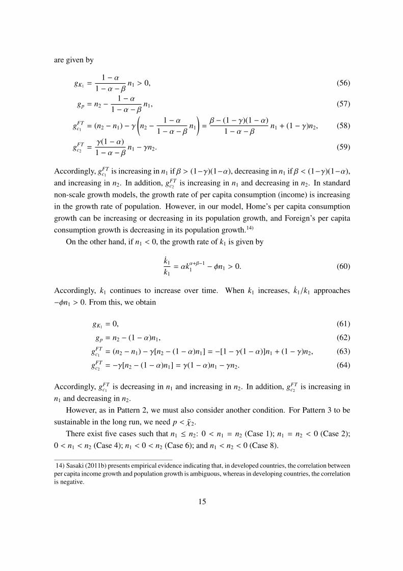
4.9 Comparisons of autarky and free trade growth rates

In this section, we compare gATc1

to gFTc1

and gATc2

to gFTc2

. The results are summarized in Table1.18)

[Table 1 around here]

With regard to per capita consumption growth, we obtain the following propositions.

Proposition 7. In Cases 1, 2, 3, and 5, both countries’ per capita consumption growthunder free trade can be equal to or more than per capita consumption growth under autarky(gAT

ci≤ gFT

ci, i = 1, 2). Other than in Cases 1 and 2, which are special cases, Pattern 2 is

realized in Cases 3 and 5.

Proposition 8. In Cases 3 and 5, the growth gap between Home and Foreign under autarkynarrows, and both countries’ growth rates are equalized by switching from autarky to freetrade (gAT

c1> gAT

c2to gFT

c1= gFT

c2). In these cases, Pattern 2 holds.

Proposition 9. In Case 4, the growth gap between Home and Foreign under autarky reverses(from gAT

c1< gAT

c2to gFT

c1> gFT

c2). In this case, Pattern 3 holds. In addition, in Case 4,

switching from autarky to free trade decreases per capita consumption growth (gATc2> gFT

c2).

18) For derivation, see Appendix A.

21

5 Conclusions

In this study, we built a two-country, two-sector, non-scale growth model and investigatedthe relationship between trade patterns and per capita consumption growth. In addition,we considered both negative and positive population growth. Our analysis yielded someinteresting results with regard to trade patterns and per capita consumption growth.

First, when the population growth of Home is higher than that of Foreign, a trade patternsuch that Home diversifies while Foreign specializes in agriculture is sustainable in the longrun. In this case, after switching from autarky to free trade, the growth gap between thecountries disappears, and both countries grow at the same per capita rate.

Second, when the population growth of Home is lower than that of Foreign, a tradepattern such that Home specializes in manufacturing while Foreign specializes in agricultureis sustainable in the long run. In this case, after switching from autarky to free trade, thegrowth gap between the two countries reverses, and Home grows faster than Foreign in percapita terms.

Third, no trade patterns are unsustainable when the population growth of a country thatproduces manufactured goods is negative. This is true irrespective of whether the populationgrowth of the other country, which does not produce manufactured goods, is positive ornegative.

Finally, under autarky, even if the population growth of Home is negative, the per capitagrowth rate is positive in the long run. However, under free trade, if the population growthof Home is negative, it can neither specialize in manufacturing nor diversify. Therefore, wecan say that whether the economy is sustainable in the long run when the population growthis negative depends on trade openness.

References

Aghion, H. and Howitt, P. (2005) “Growth with quality-improving innovations: an inte-grated framework,” in P. Aghion and S. N. Durlauf (eds.) Handbook of EconomicGrowth, ch. 2, Amsterdam: North-Holland, pp. 67–110.

Arrow, K. J. (1962) “The economic implications of learning by doing,” Review of EconomicStudies 29, pp. 155–173.

Chamon, M. and Kremer, M. (2009) “Economic transformation, population growth and thelong-run world income distribution,” Journal of International Economics 79, pp. 20–30.

22

Christiaans, T. (2008) “International trade and industrialization in a non-scale model ofeconomic growth,” Structural Change and Economic Dynamics 19, pp. 221–236.

Christiaans, T. (2011) “Semi-endogenous growth when population is decreasing,” Eco-nomics Bulletin 31 (3), pp. 2667–2673.

Dinopoulos, E. and Thompson, P. (1998) “Schumpeterian growth without scale effects,”Journal of Economic Growth 3, pp. 313–335.

Dinopoulos, E. and Sener, F. (2007) “New directions in Schumpeterian growth theory,” inH. Hanush and A. Pyca (eds.) Edgar Companion to Neo-Schumpeterian Economics,ch. 42, New York: Edward Elgar.

Dinopoulos, E. and Syropoulos, C. (2007) “Rent protection as a barrier to innovation andgrowth,” Economic Theory 32 (2), pp. 309–332.

Felbermayr, G. J. (2007) “Specialization on a technologically stagnant sector need not bebad for growth,” Oxford Economic Papers 59, pp. 682–701.

Felderer, B. (1988) “The existence of a neoclassical steady state when population growth isnegative,” Journal of Economics 48 (4), pp. 413–418.

Ferrara, M. (2011) “An AK Solow model with a non-positive rate of population growth,”Applied Mathematical Sciences 5 (25), pp. 1241–1244.

Howitt, P. (1999) “Steady endogenous growth with population and R&D inputs growth,”Journal of Political Economy 107, pp. 715–30.

Jones, C. I. (1995) “R&D-based models of economic growth,” Journal of Political Economy103, pp. 759–784.

Jones, C. I. (1999) “Growth: with or without scale effects?” American Economic Review89, pp. 139–44.

Jones, C. I. (2005) “Growth and ideas,” in P. Aghion and S. N. Durlauf (eds.) Handbook ofEconomic Growth, ch. 16, Amsterdam: North Holland, pp. 1063–1111.

Kaneko, A. (2000) “Terms of trade, economic growth, and trade patterns: a small open-economy case,” Journal of International Economics 52, pp. 169–181.

Kaneko, A. (2003) “The long-run trade pattern in a growing economy,” Journal of Eco-nomics 79 (1), pp. 1–17.

Kortum, S. (1997) “Research, patenting, and technological change,” Econometrica 65, pp.1389–1419.

Krugman, P. R. (1981) “Trade, accumulation, and uneven development,” Journal of Devel-opment Economics 8, pp. 149–161.

23

Mankiw, N. G. (2000) “The savers-spenders theory of fiscal policy,” American EconomicReview 90, pp. 120–125.

Peretto, P. F. (1998) “Technological change and population growth,” Journal of EconomicGrowth 3, pp. 283–311.

Ritschel, A. (1985) “On the stability of the steady state when population is decreasing,”Journal of Economics 45 (2), pp. 161–170.

Sasaki, H. (2011a) “Trade, non-scale growth, and uneven development,” Metroeconomica62 (4), pp. 691–711.

Sasaki, H. (2011b) “Population growth and north-south uneven development,” Oxford Eco-nomic Papers 63, pp. 307–330.

Sasaki, H. (2012) “International trade and industrialization with negative population growth,”Kyoto University, Graduate School of Economics Research Project Center DiscussionPaper Series, No. E-12-009.

Segerstrom, P. (1998) “Endogenous growth without scale effects,” American Economic Re-view 88, pp. 1290–310.

Uzawa, H. (1961) “On a two-sector model of economic growth,” Review of Economic Stud-ies 29 (1), pp. 40–47.

Wong, K.-Y., and Yip, C. K. (1999) “Industrialization, economic growth, and internationaltrade,” Review of International Economics 7, pp. 522–540.

Young, A. (1998) “Growth without scale effects,” Journal of Political Economy 106, pp.41–63.

24

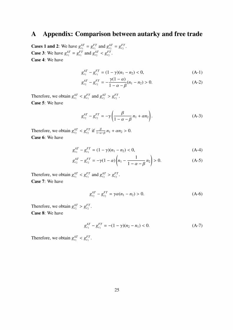
A Appendix: Comparison between autarky and free trade

Cases 1 and 2: We have gATc1= gFT

c1and gAT

c2= gFT

c2.

Case 3: We have gATc1= gFT

c1and gAT

c2< gFT

c2.

Case 4: We have

gATc1− gFT

c1= (1 − γ)(n1 − n2) < 0, (A-1)

gATc2− gFT

c2= − γ(1 − α)

1 − α − β (n1 − n2) > 0. (A-2)

Therefore, we obtain gATc1< gFT

c1and gAT

c2> gFT

c2.

Case 5: We have

gATc2− gFT

c2= −γ

(β

1 − α − β n1 + αn2

). (A-3)

Therefore, we obtain gATc2< gFT

c2if β

1−α−β n1 + αn2 > 0.Case 6: We have

gATc1− gFT

c1= (1 − γ)(n1 − n2) < 0, (A-4)

gATc2− gFT

c2= −γ(1 − α)

(n1 −

11 − α − β n2

)> 0. (A-5)

Therefore, we obtain gATc1< gFT

c1and gAT

c2> gFT

c2.

Case 7: We have

gATc2− gFT

c2= γα(n1 − n2) > 0. (A-6)

Therefore, we obtain gATc2> gFT

c2.

Case 8: We have

gATc1− gFT

c1= −(1 − γ)(n2 − n1) < 0. (A-7)

Therefore, we obtain gATc1< gFT

c1.

25

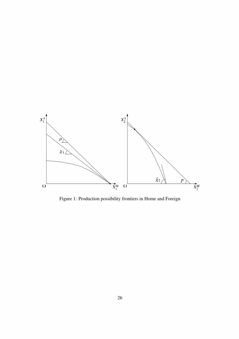
O OXM1 XM2

XA1 XA2�1p

p�2Figure 1: Production possibility frontiers in Home and Foreign

26

Tabl

e1:

Com

pari

sons

ofau

tark

yan

dfr

eetr

ade

grow

thra

tes

Cas

eC

ase

1C

ase

2C

ase

3C

ase

4♢C

ase

5C

ase

6*C

ase

7*C

ase

8*

Popu

latio

ngr

owth

0<

n 1=

n 2n 1=

n 2<

00<

n 2<

n 10<

n 1<

n 2n 2<

0<

n 1n 1<

0<

n 2n 2<

n 1<

0n 1<

n 2<

0Tr

ade

patte

rn**

2an

d3†

2an

d3†

23

23

23

Rel

atio

nshi

pgA

Tc 1=

gAT

c 2gA

Tc 1=

gAT

c 2gA

Tc 1>

gAT

c 2gA

Tc 1<

gAT

c 2gA

Tc 1>

gAT

c 2•

gAT

c 1>

gAT

c 2⋆

gAT

c 1<

gAT

c 2gA

Tc 1>

gAT

c 2

betw

een

g 1an

dg 2

gFT

c 1=

gFT

c 2gF

Tc 1=

gFT

c 2gF

Tc 1=

gFT

c 2gF

Tc 1>

gFT

c 2gA

Tc 1<

gAT

c 2••

gAT

c 1<

gAT

c 2⋆⋆

gFT

c 1=

gFT

c 2gF

Tc 1>

gFT

c 2

gAT

c 1=

gFT

c 1gA

Tc 1=

gFT

c 1gA

Tc 1=

gFT

c 1gA

Tc 1<

gFT

c 1gF

Tc 1=

gFT

c 2gF

Tc 1>

gFT

c 2gA

Tc 1=

gFT

c 1gA

Tc 1<

gFT

c 1

gAT

c 2=

gFT

c 2gA

Tc 2=

gFT

c 2gA

Tc 2<

gFT

c 2gA

Tc 2>

gFT

c 2gA

Tc 1=

gFT

c 1gA

Tc 1<

gFT

c 1gA

Tc 2>

gFT

c 2gA

Tc 2>

gFT

c 2

gAT

c 2<

gFT

c 2•

gAT

c 2>

gFT

c 2

gAT

c 2>

gFT

c 2••

Neg

ativ

egr

owth

gFT

c 1<

0gF

Tc 2<

0♠n/

agF

Tc 2<

0gF

Tc 2<

0

♢n 2<

11−α−β

n 1is

impo

sed.

*T

hese

case

sar

eun

sust

aina

ble

inth

elo

ngru

n.**

Patte

rn2

isth

eca

sein

whi

chH

ome

dive

rsifi

esan

dFo

reig

nsp

ecia

lizes

inag

ricu

lture

.Pa

ttern

3is

the

case

inw

hich

Hom

ean

dFo

reig

nsp

ecia

lize

inm

anuf

actu

ring

and

agri

cultu

re,r

espe

ctiv

ely.

†Pa

ttern

2is

obta

ined

ifγ≤

1/2,

whi

lePa

ttern

3is

obta

ined

if1/

2<γ

.♠

1−α

1−α−β

n 1<

n 2<

11−α−β

n 1.

•β

1−α−β

n 1+α

n 2>

0.••

β

1−α−β

n 1+α

n 2<

0.H

owev

er,t

his

case

isun

sust

aina

ble

inth

elo

ngru

n.⋆α

n 1+

β

1−α−β

n 2<

0.⋆⋆α

n 1+

β

1−α−β

n 2<

0

27