Position-momentum uncertainty relations in the … · Position-momentum uncertainty relations in the presence of quantum memory Fabian Furrer, Mario Berta, Marco Tomamichel, Volkher

Position-momentum uncertainty relations in the presence of quantummemoryFabian Furrer, Mario Berta, Marco Tomamichel, Volkher B. Scholz, and Matthias Christandl Citation: Journal of Mathematical Physics 55, 122205 (2014); doi: 10.1063/1.4903989 View online: http://dx.doi.org/10.1063/1.4903989 View Table of Contents: http://scitation.aip.org/content/aip/journal/jmp/55/12?ver=pdfcov Published by the AIP Publishing Articles you may be interested in Relating different quantum generalizations of the conditional Rényi entropy J. Math. Phys. 55, 082206 (2014); 10.1063/1.4892761 A transform of complementary aspects with applications to entropic uncertainty relations J. Math. Phys. 51, 082201 (2010); 10.1063/1.3477319 Higher entropic uncertainty relations for anti-commuting observables J. Math. Phys. 49, 062105 (2008); 10.1063/1.2943685 Rényi Entropy and the Uncertainty Relations AIP Conf. Proc. 889, 52 (2007); 10.1063/1.2713446 Separability Criteria from Uncertainty Relations AIP Conf. Proc. 734, 230 (2004); 10.1063/1.1834422

This article is copyrighted as indicated in the article. Reuse of AIP content is subject to the terms at: http://scitation.aip.org/termsconditions. Downloaded

to IP: 131.215.70.231 On: Thu, 29 Jan 2015 16:11:55

http://scitation.aip.org/content/aip/journal/jmp?ver=pdfcov

http://oasc12039.247realmedia.com/RealMedia/ads/click_lx.ads/www.aip.org/pt/adcenter/pdfcover_test/L-37/864763109/x01/AIP-PT/JMP_ArticleDL_122414/PT_SubscriptionAd_1640x440.jpg/47344656396c504a5a37344142416b75?x

http://scitation.aip.org/search?value1=Fabian+Furrer&option1=author

http://scitation.aip.org/search?value1=Mario+Berta&option1=author

http://scitation.aip.org/search?value1=Marco+Tomamichel&option1=author

http://scitation.aip.org/search?value1=Volkher+B.+Scholz&option1=author

http://scitation.aip.org/search?value1=Matthias+Christandl&option1=author

http://scitation.aip.org/content/aip/journal/jmp?ver=pdfcov

http://dx.doi.org/10.1063/1.4903989

http://scitation.aip.org/content/aip/journal/jmp/55/12?ver=pdfcov

http://scitation.aip.org/content/aip?ver=pdfcov

http://scitation.aip.org/content/aip/journal/jmp/55/8/10.1063/1.4892761?ver=pdfcov



http://scitation.aip.org/content/aip/proceeding/aipcp/10.1063/1.2713446?ver=pdfcov

http://scitation.aip.org/content/aip/proceeding/aipcp/10.1063/1.1834422?ver=pdfcov

JOURNAL OF MATHEMATICAL PHYSICS 55, 122205 (2014)

Position-momentum uncertainty relations in the presenceof quantum memory

Fabian Furrer,1,a) Mario Berta,2,3 Marco Tomamichel,4,5 Volkher B. Scholz,3and Matthias Christandl3,61Department of Physics, Graduate School of Science, University of Tokyo, 7-3-1 Hongo,Bunkyo-ku, Tokyo 113-0033, Japan2Institute for Quantum Information and Matter, Caltech, Pasadena, California 91125, USA3Institute for Theoretical Physics, ETH Zurich, Wolfgang-Pauli-Str. 27, 8093 Zürich,Switzerland4School of Physics, The University of Sydney, Sydney 2006, Australia5Centre for Quantum Technologies, National University of Singapore, Singapore 117543,Singapore6Department of Mathematical Sciences, University of Copenhagen, Universitetsparken 5,2100 Copenhagen, Denmark

(Received 12 October 2014; accepted 29 November 2014; published online 23 December 2014)

A prominent formulation of the uncertainty principle identifies the fundamentalquantum feature that no particle may be prepared with certain outcomes for bothposition and momentum measurements. Often the statistical uncertainties are therebymeasured in terms of entropies providing a clear operational interpretation in infor-mation theory and cryptography. Recently, entropic uncertainty relations have beenused to show that the uncertainty can be reduced in the presence of entanglementand to prove security of quantum cryptographic tasks. However, much of this recentprogress has been focused on observables with only a finite number of outcomesnot including Heisenberg’s original setting of position and momentum observables.Here, we show entropic uncertainty relations for general observables with discretebut infinite or continuous spectrum that take into account the power of an entangledobserver. As an illustration, we evaluate the uncertainty relations for position andmomentum measurements, which is operationally significant in that it implies secu-rity of a quantum key distribution scheme based on homodyne detection of squeezedGaussian states. C 2014 AIP Publishing LLC. [http://dx.doi.org/10.1063/1.4903989]

I. INTRODUCTION

Heisenberg’s original writing1 allows different and sometimes conflicting interpretations ofwhat formalization of the uncertainty relation he had in mind; in this work, we will adopt anadversarial perspective common in quantum information theory that has been fruitful in the contextof quantum cryptography. This is sometimes referred to as preparation uncertainty and goes back toKennard2 and Robertson.3

For the following, assume that either a position or a momentum measurement is to be per-formed on a quantum system prepared in an arbitrary state. An uncertainty relation then bounds theuncertainty of the measurement outcome from the perspective of an external observer (without ac-cess to the measurement device), when either the position or momentum of the particle is measured.For a particle prepared in a well-defined location, clearly the position uncertainty is low but themomentum uncertainty might be high. For a wave-like quantum system, the opposite is true. Moregenerally, Heisenberg’s uncertainty relation proclaims that, independent of the prepared state, it isimpossible that both uncertainties are small.

Kennard made this statement precise by showing that the variance of the position and mo-mentum distribution Varω[Q] and Varω[P] satisfies the famous inequality

a)[email protected]

0022-2488/2014/55(12)/122205/30/$30.00 55, 122205-1 © 2014 AIP Publishing LLC


to IP: 131.215.70.231 On: Thu, 29 Jan 2015 16:11:55

http://dx.doi.org/10.1063/1.4903989

http://dx.doi.org/10.1063/1.4903989

http://dx.doi.org/10.1063/1.4903989

http://dx.doi.org/10.1063/1.4903989

http://dx.doi.org/10.1063/1.4903989

http://dx.doi.org/10.1063/1.4903989

http://dx.doi.org/10.1063/1.4903989

http://dx.doi.org/10.1063/1.4903989

http://dx.doi.org/10.1063/1.4903989

http://dx.doi.org/10.1063/1.4903989

mailto:[email protected]































http://crossmark.crossref.org/dialog/?doi=10.1063/1.4903989&domain=pdf&date_stamp=2014-12-23

122205-2 Furrer et al. J. Math. Phys. 55, 122205 (2014)

Varω[Q] · Varω[P] ≥ 14, (1)

where throughout the paper, units are in ~ = 1. Subsequently, several formulations of the uncer-tainty relation for different measures of uncertainty have been proposed. We are particularly inter-ested in entropic formulations of the uncertainty principle,4–6 which we will discuss in more detailin Sec. II.

Nonetheless, it has been recently pointed out7 that the above picture is incomplete in the presenceof quantum entanglement. In fact, it is evident that the preparation uncertainty from the perspective ofan external observer can be reduced significantly if the observer is allowed to interact with the envi-ronment of the system. For example, imagine that an approximate Einstein-Podolsky-Rosen (EPR)entangled state8 is prepared — the continuous analog of a maximally entangled state — exhibitingstrong correlations in both position and momentum measurements. Then, the uncertainties of theoutcome of position and momentum measurements are reduced if the observer is given access to aquantum memory (respectively, the environment) storing one part of the approximate EPR state. Andin fact, the uncertainty simply vanishes in the limit of an ideal EPR state with perfect correlations.

Formally, this uncertainty reduction due to entanglement can best be quantified for a three partysituation which reveals an interesting interplay between the uncertainty principle and monogamy ofentanglement (see, e.g., Ref. 9). Suppose that two non-collaborating external observers are present,one interested in the position and the other one in the momentum measurement. Then, even thoughthey have access to disjoint parts of the environment, the total uncertainty cannot (significantly)be reduced. To exemplify this, assume that one observer’s quantum memory is in an approximateEPR state with the measured system reducing his uncertainty. Because the approximate EPR stateis pure, the other observer is uncorrelated. Moreover, the latter observer has high uncertainty sincethe measured system is in a thermal state (the partial trace of an approximate EPR state) with largerspread as the correlations of the approximate EPR state are enhanced.

In this article, we quantify this trade-off between the uncertainties of two external observers forboth discretized as well as continuous position and momentum measurements. We show these rela-tions if the uncertainties are quantified by the quantum conditional entropy, the conditional versionof the von Neumann entropy, and by conditional min- and max-entropies. We also encounter theinteresting phenomena for the quantum conditional entropy that the uncertainty bound is strictlylower than in the case of no quantum memory. This is in contrast to the finite-dimensional case.7

Similar uncertainty relations have recently also been shown by Frank and Lieb10 and by oneof the present authors.11 In the former work, the authors employ a more restrictive definition ofthe quantum conditional entropy and do not consider min- and max-entropies which are significantfor quantum key distribution. Here, we build on the latter work and use a definition which is moresuitable for systems with an infinite number of degrees of freedom. In particular, we introduce ageneral definition of the differential quantum conditional entropy in which the classical system ismodeled by a σ-finite measure space and the quantum system by an arbitrary von Neumann algebra.Moreover, we show that under weak assumptions this definition is retrieved as the limit of thecorresponding regularized discrete quantities along finer and finer discretization. This provides anoperational approach to the differential quantum conditional entropy. We also introduce differentialversions of the quantum conditional min- and max-entropies and show that they similarly emergeunder weak assumptions as the regularized limits along finer and finer discretization from theirdiscrete counterparts.

The paper is organized as follows. First, we give a non-technical discussion of the results.Then, in Sec. III, we review the algebraic formalism to describe quantum and classical systems.In Sec. IV, we introduce and discuss the differential quantum conditional entropies. The entropicuncertainty relations in the presence of quantum memory are proven in Sec. V. We discuss thespecial case of position and momentum measurements in Sec. V C, and eventually, conclude ourresults in Sec. VI.


to IP: 131.215.70.231 On: Thu, 29 Jan 2015 16:11:55


II. DISCUSSION OF THE RESULTS

In the following, we start with the differential Shannon entropy12 to measure the uncertaintyassociated to the outcomes of a position (or momentum) measurement. For the sake of the motiva-tion, we first follow an operational approach and think of the differential Shannon entropy as thelimit of the ordinary discrete Shannon entropy for finer and finer discretization. Consider a detectorthat measures if the outcome q of a position measurement falls in an interval Ik ;α B (kα, (k + 1)α]where k is an integer and α = 2−n, the interval size for some n ∈ N. The Shannon entropy of thismeasurement is then

H(Qα)ω B −∞

k=−∞ω(Ik ;α) logω(Ik ;α), (2)

where ω(Ik ;α) denotes the probability of q being observed in the interval Ik ;α when the state is ωand Qα is the random variable indicating in which interval q falls.

A straightforward way to define the differential Shannon entropy would be to use the limitlimα→0[H(Qα)ω + log α]. The additional term log α elucidates the necessity of renormalization asthe probability ω(Ik ;α) scales with the length of the interval, α. However, due to ambiguities thatcan arise by the discretization and that one has to show the existence of the limit, it is moreconvenient to use the closed formula

h(Q)ω B −

dq Pω(q) log Pω(q) (3)

in order to define the Shannon entropy. Here, Pω(q) is the induced probability density when measur-ing the position of the state ω. It is clear that the two definitions coincide if for instance Pω iscontinuous. In the following, we denote the similarly defined differential entropy for the momentumdistribution by h(P)ω.

Evaluating the differential entropy for Gaussian wave packets with variance σ2 yields h(Q)ωg =12 log(2πeσ2) and h(P)ωg =

12 log eπ

2σ2 , respectively. Independently, Białynicki-Birula and Myciel-ski5 and Beckner6 showed the entropic uncertainty relation

h(Q)ω + h(P)ω ≥ log(eπ). (4)

This bound was originally derived for pure states, but also holds for mixed states (see, e.g., Ref. 13).And as for Kennard’s relation, Gaussian wave packets achieve equality.

These concepts can be extended to include the effects of a quantum memory. For this purpose,we first need to define a measure that characterizes the uncertainty for an observer holding quantumside information — the differential quantum conditional von Neumann entropy. Let us consider twoseparate physical systems, A and B, in a joint state ωAB. We use the convention that A is the systemto be measured and B is a quantum system held by an observer. A natural definition of the differen-tial quantum conditional von Neumann entropy would again be limα→0

H(Qα |B)ω + log α

, where

Qα has the same meaning as above and H(Qα |B)ω is the discrete (quantum) conditional von Neu-mann entropy. For finite-dimensional systems as well as in the work by Frank and Lieb,10 the condi-tional von Neumann entropy of a classical variable X conditioned on quantum side-informationB is defined via the chain rule H(X |B) = H(X B) − H(B). However, this is inconvenient for ourconsiderations here as we want to consider a quantum system B that is fully general in which caseboth H(X B) and H(B) might be infinite whereas the conditional uncertainty, expressed through thequantum conditional von Neumann entropy H(X |B), is still well-defined and finite. We thereforedefine the quantum conditional von Neumann entropy as

H(Qα |B)ω B −∞

k=−∞D�ωk ;α

B

�ωB

�, (5)

where D(·∥·) is Umegaki’s quantum relative entropy,14 ωB is the marginal state on B, and ωk ;αB is

the sub-normalized marginal state on B when q is measured in Ik ;α. Note the simple relation ωB =k ω

k ;αB . We emphasize here that in this definition, the system B can be any quantum or classical

system including continuous classical systems or quantized fields. Moreover, in the finite-dimensional


to IP: 131.215.70.231 On: Thu, 29 Jan 2015 16:11:55


case, the quantum relative entropy for two density matrices ρ and σ is given by D(ρ∥σ) = trρ log ρ− trρ logσ such that one retrieves the common definition H(X |B) = H(X B) − H(B).

Similar to the case without side information, it is more convenient to define the differentialconditional von Neumann entropy as a closed expression. Hence, as a natural generalization of for-mula (5), we define the differential quantum conditional von Neumann entropy as (see Definition 4)

h(Q|B)ω = − ∞

−∞dq D

�ω

qB

�ωB

�, (6)

where ωqB is the conditional state density on the system B in the sense that

Ik ;α

dqωqB = ω

k ;αB . In

Proposition 5, we then show that if −∞ < h(Q|B)ω and H(Qα |B)ω < ∞ are satisfied for an arbitraryα > 0, it follows that

h(Q|B)ω = limα→0

H(Qα |B)ω + log α

. (7)

Next, let us state the obtained uncertainty relations in terms of the quantum conditional vonNeumann entropies. First, we consider measurements with finite spacing δq for q and δp for p onthe A system of a tripartite state ωABC. We then find that, for all states,

H(Qδq |B)ω + H(Pδp |C)ω ≥ − log c(δq, δp) , (8)

with

c(δq, δp) = maxk,l

∥

Qk[δq]

Pl[δp]∥, (9)

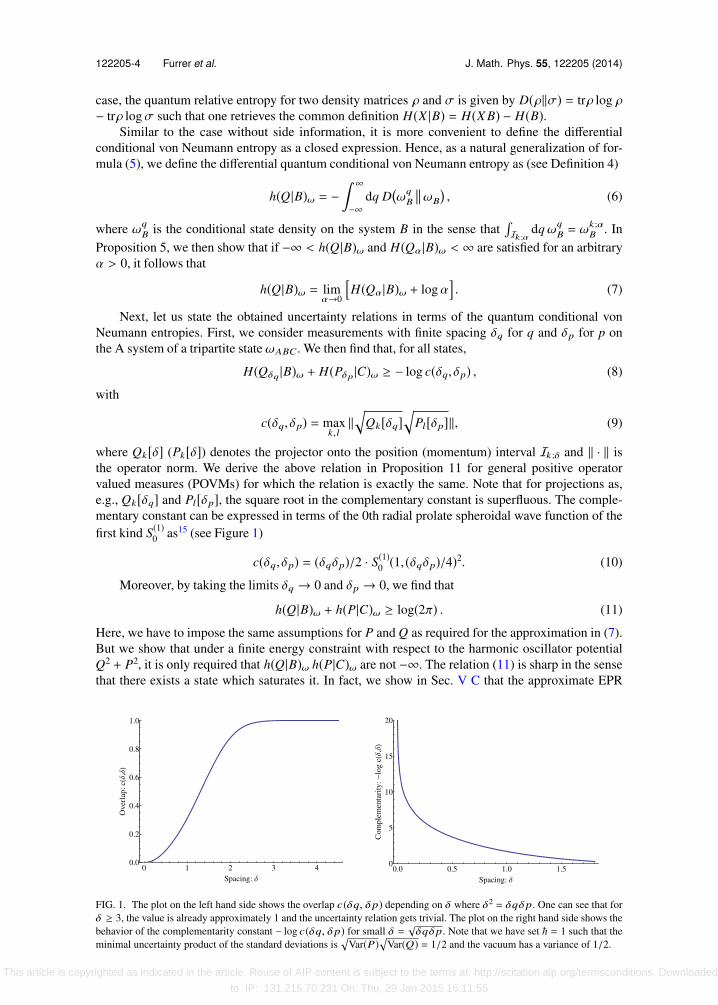
where Qk[δ] (Pk[δ]) denotes the projector onto the position (momentum) interval Ik ;δ and ∥ · ∥ isthe operator norm. We derive the above relation in Proposition 11 for general positive operatorvalued measures (POVMs) for which the relation is exactly the same. Note that for projections as,e.g., Qk[δq] and Pl[δp], the square root in the complementary constant is superfluous. The comple-mentary constant can be expressed in terms of the 0th radial prolate spheroidal wave function of thefirst kind S(1)

0 as15 (see Figure 1)

c(δq, δp) = (δqδp)/2 · S(1)0 (1, (δqδp)/4)2. (10)

Moreover, by taking the limits δq → 0 and δp → 0, we find that

h(Q|B)ω + h(P|C)ω ≥ log(2π) . (11)

Here, we have to impose the same assumptions for P and Q as required for the approximation in (7).But we show that under a finite energy constraint with respect to the harmonic oscillator potentialQ2 + P2, it is only required that h(Q|B)ω h(P|C)ω are not −∞. The relation (11) is sharp in the sensethat there exists a state which saturates it. In fact, we show in Sec. V C that the approximate EPR

FIG. 1. The plot on the left hand side shows the overlap c(δq, δp) depending on δ where δ2 = δqδp. One can see that forδ ≥ 3, the value is already approximately 1 and the uncertainty relation gets trivial. The plot on the right hand side shows thebehavior of the complementarity constant − log c(δq, δp) for small δ =

√δqδp. Note that we have set ~ = 1 such that the

minimal uncertainty product of the standard deviations is

Var(P)Var(Q) = 1/2 and the vacuum has a variance of 1/2.


to IP: 131.215.70.231 On: Thu, 29 Jan 2015 16:11:55


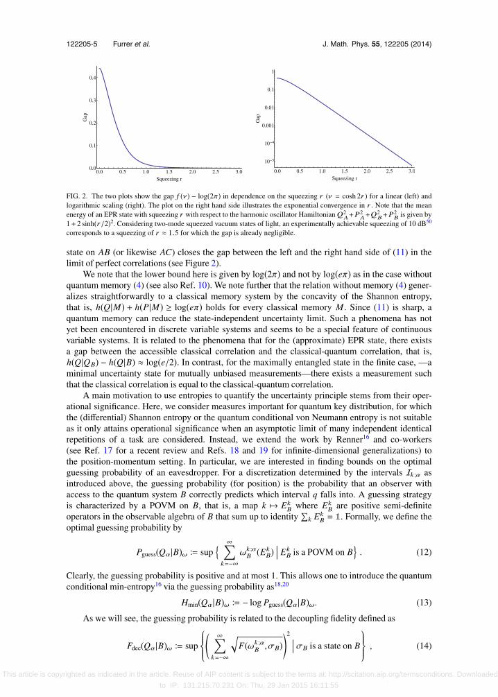
FIG. 2. The two plots show the gap f (ν) − log(2π) in dependence on the squeezing r (ν = cosh 2r ) for a linear (left) andlogarithmic scaling (right). The plot on the right hand side illustrates the exponential convergence in r . Note that the meanenergy of an EPR state with squeezing r with respect to the harmonic oscillator Hamiltonian Q2

A+P2A+Q

2B+P

2B is given by

1+ 2 sinh(r/2)2. Considering two-mode squeezed vacuum states of light, an experimentally achievable squeezing of 10 dB50

corresponds to a squeezing of r ≈ 1.5 for which the gap is already negligible.

state on AB (or likewise AC) closes the gap between the left and the right hand side of (11) in thelimit of perfect correlations (see Figure 2).

We note that the lower bound here is given by log(2π) and not by log(eπ) as in the case withoutquantum memory (4) (see also Ref. 10). We note further that the relation without memory (4) gener-alizes straightforwardly to a classical memory system by the concavity of the Shannon entropy,that is, h(Q|M) + h(P|M) ≥ log(eπ) holds for every classical memory M . Since (11) is sharp, aquantum memory can reduce the state-independent uncertainty limit. Such a phenomena has notyet been encountered in discrete variable systems and seems to be a special feature of continuousvariable systems. It is related to the phenomena that for the (approximate) EPR state, there existsa gap between the accessible classical correlation and the classical-quantum correlation, that is,h(Q|QB) − h(Q|B) ≈ log(e/2). In contrast, for the maximally entangled state in the finite case, —aminimal uncertainty state for mutually unbiased measurements—there exists a measurement suchthat the classical correlation is equal to the classical-quantum correlation.

A main motivation to use entropies to quantify the uncertainty principle stems from their oper-ational significance. Here, we consider measures important for quantum key distribution, for whichthe (differential) Shannon entropy or the quantum conditional von Neumann entropy is not suitableas it only attains operational significance when an asymptotic limit of many independent identicalrepetitions of a task are considered. Instead, we extend the work by Renner16 and co-workers(see Ref. 17 for a recent review and Refs. 18 and 19 for infinite-dimensional generalizations) tothe position-momentum setting. In particular, we are interested in finding bounds on the optimalguessing probability of an eavesdropper. For a discretization determined by the intervals Ik ;α asintroduced above, the guessing probability (for position) is the probability that an observer withaccess to the quantum system B correctly predicts which interval q falls into. A guessing strategyis characterized by a POVM on B, that is, a map k → Ek

B where EkB are positive semi-definite

operators in the observable algebra of B that sum up to identity

k EkB = 1. Formally, we define the

optimal guessing probability by

Pguess(Qα |B)ω B sup ∞k=−∞

ωk ;αB (Ek

B) �� EkB is a POVM on B

. (12)

Clearly, the guessing probability is positive and at most 1. This allows one to introduce the quantumconditional min-entropy16 via the guessing probability as18,20

Hmin(Qα |B)ω B − log Pguess(Qα |B)ω. (13)

As we will see, the guessing probability is related to the decoupling fidelity defined as

Fdec(Qα |B)ω B sup*,

∞k=−∞

F(ωk ;α

B ,σB)+-

2�� σB is a state on B

, (14)


to IP: 131.215.70.231 On: Thu, 29 Jan 2015 16:11:55


where F(·, ·) is Uhlmann’s fidelity21 and we recall that ωk ;αB is not normalized. The decoupling fidel-

ity, Fdec(Qα |B)ω, is a measure of how much information the marginal state on B contains about Qα.If the state is independent, that is, if B does not contain any information about Qα, the decouplingfidelity takes its maximum value as Fdec(Qα) = �∞

k=−∞ωA(Ik ;α)�2. The latter expression grows

with the support of the distribution, and is positive but not necessarily finite. Similarly, as in the caseof the guessing probability, we can associate an entropic quantity to the decoupling fidelity, which isknown as the quantum conditional max-entropy18,20

Hmax(Qα |B)ω = log Fdec(Qα |B)ω. (15)

In this work, we introduce the differential guessing probability and the differential decouplingfidelity, and accordingly, the differential quantum conditional min- and max-entropies. We definethem by straightforwardly generalizing the infinite sums in (12) and (14) to integrals

pguess(Q|B)ω B sup ∞

−∞dq ωq

B(EqB)

��q → Eq

B is a POVM on B,

fdec(Q|B)ω B sup

( ∞

−∞dq

F(ωq

B,σB))2 ��

σB is a state on E.

In analogy to before, the differential quantum conditional min- and max-entropies are then definedas hmin(Q|B)ω = − log pguess(Q|B)ω and hmax(Q|B)ω = log fdec(Q|B)ω (see Definition 6). Similar asfor the quantum conditional von Neumann entropy, we show that the differential quantum condi-tional min- and max-entropies can be retrieved in the limit of finer and finer discretization (seeProposition 7)

hmin(Q|B)ω = limα→0

(Hmin(Qα |B)ω + log α

), (16)

hmax(Q|B)ω = limα→0

(Hmax(Qα |B)ω + log α

), (17)

where the notation is as in (7) and (17) holds if Hmax(Qα |B)ω < ∞ for an arbitrary α > 0.The above quantities allow us to formulate a different entropic uncertainty relation, which

generalizes the relation in Ref. 22 to a countable or continuous set of outcomes and general sideinformation. For an arbitrary tripartite system in state ωABC and finite spacing δp, δq, we find thatPguess(Qδq |B)ω ≤ c(δq, δp) · Fdec(Pδp |C)ω, where c(δq, δp) is same as in (8). Expressed in terms ofentropies, this is equivalent to

Hmin(Qδq |B)ω + Hmax(Pδp |C)ω ≤ c(δq, δp). (18)

We prove the above relation for arbitrary POVM measurements in Proposition 9.The analogous relation in the continuous limit is obtained via (16) and (17) and reads

hmin(Q|B)ω + hmax(P|C)ω ≥ log(2π) . (19)

Note that we have to impose that Hmax(Pα |B)ω < ∞ for an arbitrary α > 0. But as shown inLemma 8, this is true if the second moments of the momentum distribution are finite. Both of theserelations can be made sharp even in the absence of any correlation between q and B and p andC. We show in Proposition 14 that for any δp, δq > 0, the discretized version (18) gets tight for astate with no uncertainty in the momentum degree, i.e., a state with a momentum distribution withsupport only on one of the intervals of length δp. However, tightness of (19) cannot be inferred fromthis observation because a hypothetical limit state must have an exactly defined momentum which isunphysical. But as already shown in Ref. 13, tightness of (19) is given for pure Gaussian states.

III. PRELIMINARIES

A. Algebraic description of physical systems

Opposite to the standard description of quantum mechanics where the structure of the system isrelated to a Hilbert space, the basic objects in the algebraic approach are the observables or, respec-tively, the algebra generated by the possible observables. It is reasonable to close the observable


to IP: 131.215.70.231 On: Thu, 29 Jan 2015 16:11:55


algebra with respect to the topology which corresponds to taking quantum mechanical expectationvalues, that is, the σ-weak topology. More precisely, the σ-weak topology on B(H ) is the locallyconvex topology induced by the semi-norms A → |tr(τA)| for trace-class operators τ ∈ B(H ), seeRef. 23, Chap. 2.4.1. Such an algebra is called a von Neumann algebra: a von Neumann algebraMis a σ-weakly closed subalgebra of the linear, bounded operators B(H ) on some Hilbert space H .The algebraic approach has for instance the benefit that one can treat classical and quantum systemson the same footing. We start with specifying general quantum systems.

1. Quantum systems

We associate to every quantum system a von Neumann algebra M acting on a Hilbert spaceH . The set of linear, normal (i.e., σ-weakly continuous), and positive functionals onM is denotedby P(M). The set of sub-normalized states S≤(M) is defined as the elements in P(M) satisfyingω(1) ≤ 1, where 1 denotes the identity element in M. Elements ω ∈ S≤(M) with ω(1) = 1 arecalled (normalized) states, and the corresponding set is denoted by S(M). If M � B(H ), thenthere exists a one to one correspondence between states onM and density matrices onH . We thenhave for every ω ∈ S(M), a unique positive trace-one operator ρ on H , such that for all E ∈ M,ω(E) = tr[ρE]. We denote the set of density operators onH by S(H ).

A multipartite system is a composite of different local subsystems A,B,C associated withmutually commuting von Neumann algebras MA,MB,MC acting on the same Hilbert space H .The combined system is denoted byMABC and is given by the von Neumann algebra generated bythe individual subsystems, that is,MABC =MA ∨MB ∨MC is the σ-weak closure of the algebra{abc : a ∈ MA,b ∈ MB,c ∈ MC}. If it is not clear from context, we label the correspondence ofstates, operators, and algebras to different subsystems by lower indexes.

By the Gelfand-Naimark-Segal (GNS) construction every ω ∈ S≤(M) admits a purificationthat is a triple (K , π, ξω), K being a Hilbert space, π being a representation ofM on K , and a sub-normalized vector ξω ∈ H such that ω(x) = ⟨ξω |π(x)ξω ⟩ for all x ∈ M (see, e.g., Ref. 23, Chap.2.3.3). We often speak of the commutant π(M)′ of π onK as the purifying system.

The space P(M) can be equipped with two different, albeit equivalent notions of distance.21,24

The first one is the usual norm induced byM and defined for ω ∈ P(M) as

∥ω∥ = supE∈M,∥E∥≤1

|ω(E)|2. (20)

ForM = B(H ) and density matrices, this corresponds to the usual trace-distance. The second oneis called the fidelity and was introduced by Uhlmann.21 The fidelity for ω,σ ∈ S≤(M) is defined as

F(ω,σ) = sup | ⟨ξω |ξσ ⟩|2 , (21)

where the supremum runs over all purifications of ω and σ being defined with respect to the sameHilbert space. This is a non-empty set since there exists a Hilbert space K and a representation π ofM onK , called standard form, such that every state onM has a purification onK , Ref. 25, Chap. 9.

2. Classical systems

A classical system is specified by the property that all possible observables commute, and canthus be described by an abelian von Neumann algebra. This perspective allows one to use the samedefinitions for states on classical systems as defined for quantum systems in the previous paragraph.Since classical systems will play a major role in the sequel, we discuss them in more detail.

For the sake of illustration, we start with countable classical systems denoted by X . In thefollowing, we denote quantum systems by indexes A,B,C and classical systems by indexes X,Y, Z .In the classical case, we use X,Y, Z to specify the subsystem as well as the range of the classicalvariable. The von Neumann algebra corresponding to a countable classical system X is ℓ∞(X), thatis, the set of functions from X to C equipped with the supremum norm. Here, one can think ofex = (δx,k)k as the measurement operator corresponding to the outcome x ∈ X . A classical stateis then a normalized positive functional ωX on ℓ∞(X), which can be identified with a probability


to IP: 131.215.70.231 On: Thu, 29 Jan 2015 16:11:55


distribution on X , that is, ωX ∈ ℓ1(X). It is often convenient to embed the classical system ℓ∞(X)into the quantum system with Hilbert space dimension X as the algebra of diagonal matrices withrespect to a fixed basis {|x⟩}x∈X. A classical state ωX can then be represented by a density operator

ρωX=

x

ωX(x)|x⟩⟨x | , (22)

such that the probability distribution can be identified with the eigenvalues of the correspondingdensity operator.

Let us now go a step further and consider classical systems with continuous degrees offreedom. In order to define such systems properly, we start with (X,Σ, µ) a measure space withσ-algebra Σ, and measure µ. In the following, we will always assume that the measure space isσ-finite. The von Neumann algebra of the system is given by the essentially bounded functionsdenoted by L∞(X). A classical state on X is defined as a normalized positive and normal functionalon L∞(X), and may be identified with an element of the integrable complex functions L1(X), whichis almost everywhere non-negative and satisfies

X

ωX(x)dµ(x) = 1 . (23)

Such functions in L1(X) are also called probability distributions on X . The most prominent exampleof a continuous classical system is X = R with the usual Lebesgue measure. This is of course therelevant classical system in the case of position or momentum measurement.

Note that the case of a discrete classical system is obtained if the measure space X is discreteand equipped with the equally weighted discrete measure µ(I) =

x∈I 1 for I ⊂ X . In the discretecase, (22) defines a representation of a classical state as a diagonal matrix of trace-one on the Hilbertspace with dimension equal to the classical degrees of freedom. However, in the case of continuousvariables, this representation is not possible if we demand that the image is a valid density operator.This is easily seen from the fact that every density operator is by definition of trace class, and hence,has discrete spectrum.

3. Classical-quantum systems

Let us take a closer look at bipartite systems consisting of a classical part X and a quantum partB. For a countable classical part X , the combined system is described by the von Neumann algebra(see, e.g., Ref. 26, Chap. 6.3)

MXB = ℓ∞(X) ∨MB � ℓ

∞(X) ⊗MB � ℓ∞(X,MB) = { f : X → MB : sup

x∥ f (x)∥ ≤ ∞}. (24)

A state on MXB is called a classical-quantum state and can be written as ωXB = (ωxB)x∈X with

ωxB ∈ S≤(MB) and

xω

xB(1) = 1. If the quantum system B is given by the set of all bounded linear

operators on a Hilbert spaceHB, we can represent ωXB uniquely by the density operator

ρωXB=

x

|x⟩⟨x | ⊗ ρωxB. (25)

It is now straightforward to generalize the above introduced classical-quantum systems from count-able to continuous classical systems. The combined system is then described by the von Neumannalgebra (see, e.g., Ref. 26, Chap. 6.3)

MXB = L∞(X) ∨MB � L∞(X) ⊗MB � L∞(X,MB) , (26)

where L∞(X,MB) denotes the space of essentially bounded functions with values in MB. Thenormal, positive functionals on MXB are given by elements in L1(X,P(MB)), and states can beidentified with integrable functions ωXB on X with values in P(MB) satisfying the normalizationcondition

X

ωxB(1)dµ(x) = 1 . (27)


to IP: 131.215.70.231 On: Thu, 29 Jan 2015 16:11:55


In analogy to the discrete case, we write the argument of the map ωXB as an upper index. The eval-uation of ωXB on an element EXB ∈ L∞(X,MB) is computed by ωXB(EXB) =

X ω

xB(EB(x))dµ(x).

For further details, we refer to Ref. 27, Chap. 4.6 and 4.7.

B. Channels, measurements, and post-measurement states

We call an evolution of a system a channel. As we work with von Neumann algebras it is conve-nient to define channels as maps on the observable algebra, which is also called the Heisenbergpicture. A channel from system A to system B described by von Neumann algebrasMA andMB,respectively, is given by a linear, normal, completely positive, and unital map E :MB → MA. Alinear mapΦ : N → M between two von Neumann algebras is called completely positive, if the map(idn ⊗ Φ) : Mn ⊗ N → Mn ⊗M is positive for all n ∈ N. The map is called unital, if φ(1N) = 1M.Note thatMA andMB can be either a classical or a quantum system. If both systems are quantum(classical), we call the channel a quantum (classical) channel.

A measurement with outcome range X is a channel which maps L∞(X) to a von NeumannalgebraMA. Its predual then maps states of the quantum system A to states of the classical systemX . We denote the set of all measurements E : L∞(X) → MA by Meas(X,MA). If X is countable,we can identify a measurement E : ℓ∞(X) → MA by a collection of positive operators Ex = E(ex)(x ∈ X) satisfying

x Ex = 1 (we denote by ex the sequence with 1 at position x and 0 elsewhere).

More generally, given a σ-finite measure space (X,Σ, µ) and the associated algebra L∞(X), themapping O → χO → E(χO), for O ∈ Σ, χO being its indicator function, defines a measure on Xwith values in the positive operators ofMA. Note that therefore our definition coincides with usualdefinition of a measurement as a positive operator valued measure, Ref. 28, Chap. 3.1. We define thepost-measurement state obtained when measuring the state ωA ∈ S(MA) with EX ∈ Meas(X,MA)by the concatenation ωX = ωA ◦ EX, that is, ωX( f ) = ωA(EX( f )) for f ∈ L∞(X). Since ωA andEX are normal, so is ωX, such that ωX is an element of the predual of L∞(X), which is L1(X).Hence, the obtained post measurement state is a proper classical state and can be represented by aprobability distribution on X .

In the following, we are particularly interested in the situation where we start with a bipar-tite quantum system MAB, and measure the A-system with some EX ∈ Meas(X,MA). The post-measurement state is then given by ωXB = ωAB ◦ EX. Similarly, as in the case of a trivial B-system,one can show that the state ωXB is a proper classical-quantum state on L∞(X) ⊗MB as introducedin the previous paragraph.

C. Discretization of continuous classical systems

Let us consider a classical system L∞(X) with (X,Σ, µ) a σ-finite measure space, where X isalso equipped with a topology. The aim is to introduce a discretization of X into countable measur-able sets along which we later show the approximation of the differential quantum conditional vonNeumann entropy and the differential quantum conditional min- and max-entropies.

We call a countable set P = {Ik}k ∈Λ (Λ any countable index set) of measurable subsets Ik ∈ Σa partition of X if X =

k Ik, µ(Ik ∩ Il) = δkl · µ(Ik), µ(Ik) < ∞, and the closure Ik is compact for

all k ∈ Λ. If µ(Ik) = µ(Il) for all k, l ∈ Λ, we call P a balanced partition, and denote µ(P) = µ(Ik).Note that the property µ(Ik ∩ Il) = δkl · µ(Ik) implies that the step functions associated to a fixedpartition form a subalgebra of all essentially bounded functions on X . If for two partitions P1, P2,all sets of P1 are subsets of elements in P2, we say that P2 is finer than P1 and write P2 ≤ P1.A family of partitions {Pα}α∈∆ with ∆ a discrete index set approaching zero such that each Pαis balanced, Pα ≤ Pα′ for α ≤ α′, µ(Pα) = α, and

α Pα generates Σ is called an ordered dense

sequence of balanced partitions. For simplicity, we usually omit the index set ∆.

Definition 1. We call an ordered dense sequence of balanced partitions {Pα} of a measurespace (X,Σ, µ) a coarse graining of X . A quadruple (X,Σ, µ,{Pα}) is called a coarse grainedmeasure space if the measure space is σ-finite and {Pα} is a coarse graining of X .


to IP: 131.215.70.231 On: Thu, 29 Jan 2015 16:11:55


Note that not every σ-finite measure space admits a coarse graining in the sense of the abovedefinition. As a simple example of a measure space that admits a coarse graining consider a discretespace with the counting measure where each partition consists of sets with measure at least one.In the case that X = R, Σ the Borel σ-algebra, and µ the Lebesgue measure, a coarse graining canbe easily constructed. For a positive real number α, let us take a partition Pα of R into intervalsIk = [kα, (k + 1)α], k ∈ Z, with µ(Pα) = α as introduced in Sec. II. Choosing for α the sequence1

2n , n ∈ N then gives rise to a coarse graining.

Remark 2. Every Lebesgue measurable subset X ⊂ R equipped with the Lebesgue measurerestricted to X admits a coarse graining.

For a classical-quantum system MXB = L∞(X) ⊗MB, and a partition P = {Ik}k ∈Λ of X , wecan define the discretized state ωXPB ∈ S(ℓ∞(Λ) ⊗MB) of ωXB ∈ S(MXB) by

ωXPB�(bk)� =

k ∈Λ

Ik

ωxB(bk) dµ(x) =

k ∈Λ

ωP,kB (bk) , (28)

where (bk) ∈ ℓ∞(Λ) ⊗MB. The new classical system induced by the partition is denoted by XP and it isclear that XP � Λ. In a similar way, we define the discretization of a measurement E ∈ Meas(X,MA)with respect to a partitionP = {Ik}k ∈Λ as the element EP ∈ Meas(XP,MA) determined by the collec-tion of positive operators

EPk = E(χIk) , (29)

where χIk denotes the indicator function of Ik. Note that the concept of a discretized measurementand a discretized state are compatible in the sense that the post-measurement state obtained from thediscretized measurement EP is equal to the one which is obtained where one first measures E andthen discretizes the state. Hence, we have that ωXPB = ωAB ◦ EP if ωXB = ωAB ◦ E.

IV. QUANTUM CONDITIONAL ENTROPY MEASURES

A. Quantum conditional von Neumann entropy

In order to motivate our definition of the differential quantum conditional von Neumann entropy,let us first recall the situation for discrete finite classical systems and finite-dimensional Hilbert spaces.For a classical-quantum density operator ρXB =

x px |x⟩⟨x |X ⊗ ρxB, the conditional von Neumann

entropy is defined as H(X |B)ρ = H(X B)ρ − H(B)ρ, where H(X B)ρ = −tr[ρXB log ρXB] denotes thevon Neumann entropy. In the following, we use that the conditional von Neumann entropy can alsobe rewritten as

H(X |B)ρ = −x

tr�pxρ

xB (log pxρ

xB − log ρB)� = −

x

D(pxρxB∥ρB) , (30)

where the quantum relative entropy of two density matrices ρ and σ acting on a finite-dimensionalHilbert spaceH is defined as (see, e.g., Ref. 29)

D(ρ∥σ) = tr[ρ log ρ] − tr[ρ logσ], (31)

in the case where the support of ρ is contained in the support of σ, and ∞ else. Writing the condi-tional von Neumann entropy in terms of the quantum relative entropy is motivated by the fact thatthe latter has a well behaved extension to states on von Neumann algebras which was introduced byAraki30 and further studied by Petz and various authors (see Ref. 31 and references therein). Thisgeneralization can be understood in the finite-dimensional case by writing

D(ρ∥σ) = trρ1/2 log

�∆(ρ/σ)�ρ1/2

, (32)

where the so-called spatial derivative is defined as ∆(ρ/σ) = L(σ−1)R(ρ), where L(a) and R(a)denote the left and right multiplication by an element a ∈ B(H ), respectively. Here, σ−1 denotesthe pseudo inverse on the support of σ. Note that ∆(ρ/σ) defines a linear positive operator acting


to IP: 131.215.70.231 On: Thu, 29 Jan 2015 16:11:55


on the Hilbert space HS(H ) of Hilbert-Schmidt operators on H . We emphasize that the mappingπ : a → L(a), a ∈ B(H ) defines a representation of the algebra B(H ) on the Hilbert space HS(H ).Before discussing the spatial derivative on von Neumann algebras, we first consider its propertiesin the case of density operators (see also Ref. 29, Chap. 3.4). The spatial derivative may then bedefined by the quadratic form

q : a → trρR(σ− 1

2 a)R(σ− 12 a)∗ = tr

�ρa∗σ−1a

�, (33)

where again R(σ− 12 a) is the right multiplication by σ−

12 a. The sesquilinear form s : (a,b) → tr

[a∗∆(ρ/σ)(b)] defining the positive linear operator ∆(ρ/σ) is derived from q by the polarizationidentity s(a,b) = 1

4 (q(a + b) − q(a − b) + iq(a − ib) − iq(a + ib)). The operator R(σ− 12 a)R(σ− 1

2 a)∗commutes with all operators acting by left multiplication, and hence is an element of the commutant ofπ(B(H )). This characterization of the spatial derivative can be generalized to states on von Neumannalgebras.

For a von Neumann algebra M ⊆ B(H ), let (ξσ, πσ,Hσ) be the GNS-triple associated withσ ∈ P(M). For vectors η in the set { η ∈ H : ∥aη∥ ≤ cησ(a∗a), a ∈ M, cη > 0 } with closureequal to the support of σ, we may define a linear bounded operator fromHσ toH by

rσ(η) : xξσ → xη . (34)

Note that the GNS construction ensures that the linear span of vectors of the form xξσ, x ∈ Mare dense in Hσ. If the Hilbert spaces Hσ and H are isomorphic and η = cxξσ for c ∈ M ′, thenrσ(η) = c. Moreover, the operator rσ(η)rσ(η)∗ is always an element of M ′. Let now ω be a stateonM, which is implemented by a vector ξ ∈ H , that is, ξ is a purifying vector of ω. The vector ξalso defines a state ω′ξ on the commutantM ′ by ω′ξ(y) = ⟨ξ |yξ ⟩ for y ∈ M ′. We define the spatialderivative ∆(ω′ξ/σ) as the self-adjoint operator associated with the quadratic form onH given by

q : η → ω′ξ(rσ(η)rσ(η)∗) . (35)

For a detailed derivation of its properties, see Ref. 25, Chap. 9.3 and Ref. 31, Chap. 4, andreferences therein. In analogy with the finite-dimensional case, we can now define the quantumrelative entropy in terms of this operator (following Araki30).

Definition 3. LetM ⊆ B(H ) be a von Neumann algebra acting on a Hilbert spaceH ,ω ∈ S(M)implemented by a vector ξ ∈ H , and σ ∈ P(M). If ξ is in the support of σ, then the quantum relativeentropy of ω with respect to σ is defined as

D(ω∥σ) = ⟨ξ | log(∆(ω′ξ/σ)

)ξ⟩ . (36)

The logarithm of the possibly unbounded operator ∆(ω′ξ/σ) is defined via the functional calculus. Ifξ is not in the support of σ, we set D(ω∥σ) = ∞.

It can be shown that the quantum relative entropy is independent of the particular choice of somepurifying vector ξ of ω, see the discussion in Ref. 31, Chap. 5 together with Ref. 32. We define nowthe differential quantum conditional von Neumann entropy as the integral version of (30). For laterpurposes, we also include an additional finite-dimensional quantum system.

Definition 4. Let MXAB = L∞(X) ⊗ B(HA) ⊗MB with (X,Σ, µ, ) a σ-finite measure space,HA a finite-dimensional Hilbert space, MB a von Neumann algebra, and ωXAB ∈ S≤(MXAB).Then, the conditional von Neumann entropy of X A given B is defined as

h(X A|B)ω = −

D(ωxAB∥trA ⊗ ωB) dµ(x), (37)

where trA is the trace onHA.

In the following, we use lower case letter h(X |B)ω if X is a continuous measure space and useuppercase letter, H(X |B)ω, if X is discrete. In the latter case of a discrete measure space, we recover


to IP: 131.215.70.231 On: Thu, 29 Jan 2015 16:11:55


the formula in (30) with now a possible infinite sum

H(X |B)ω = −x∈X

D(pxωxB∥ωB) . (38)

The following statement shows that the differential quantum conditional von Neumann entropycan be retrieved from the regularized version of its discrete counterpart in the limit of finer and finercoarse grainings.

Proposition 5. LetMXB = L∞(X) ⊗MB withMB a von Neumann algebra and (X,Σ, µ,{Pα})a coarse grained measure space. Consider ωXB ∈ S(MXB) such that −∞ < h(X |B)ω, and assumethat there exists α0 > 0 for which H(XPα0

|B)ω < ∞. Then, it follows that

h(X |B)ω = limα→0

�H(XPα |B)ω + log α

�, (39)

where ωXPαB is defined as in (28). Furthermore, if h(X)ω < ∞, then it follows that

h(X |B)ω = h(X)ω − D(ωXB∥ωX ⊗ ωB) . (40)

We note that in Ref. 33, the conditional von Neumann entropy was defined as in (40) forωAB ∈ S

�B(HA ⊗ HB)� with H(A)ω < ∞, and separable Hilbert spacesHA andHB.

Proof. We first write the integral as a series of integrals over a covering {X k}∞k=0 of X by

compact measurable sets with µ(X k ∩ X l) = 0 for k , l. Using that the Lebesgue integral canbe split over positive and negative parts of the integrand, we can use the monotone convergencetheorem to obtain

− h(X |B)ω = limn→∞

nk=1

Xk

D(ωxB∥ωB) dµ(x). (41)

For a fixed k, it follows from disintegration theory, Ref. 27, Chap. IV.7, thatXk

D(ωxB∥ωB) dx = D(ωXB∥µXk ⊗ ωB) , (42)

where µXk denotes the restriction of the Lebesgue measure on X k. Note that µXk is now a positivefinite functional such that we can apply the approximation result for the quantum relative entropyof states on a von Neumann algebra along a net of increasing subalgebras in L∞(X k) (Lemma 28).In particular, we take the net of subalgebras given by the step functions corresponding to the fixedpartitions Pk

α obtained by restricting Pα to X k. We assume here that the covering {Xk} is taken suchthat it is compatible with the partitions Pα for a small enough α such that Pk

α is balanced as well.Note that such a covering exists since one can for instance take the sets of a fixed partition Pα for alarge enough α. Let us denote the corresponding alphabet of the induced discrete and finite abelianalgebra by X k

α. Hence, we obtain that

− h(X |B)ω = limn→∞

limα→0

nk=1

D(ωXkαB

∥µXkα⊗ ωB) , (43)

where ωXkαB

and µXkα⊗ ωB are states in ℓ∞(X k

α) ⊗MB and defined as in (28). We therefore havethat µXk

α= α1, where the identity is the one in ℓ∞(X k

α), and it follows by an elementary property ofthe quantum relative entropy (Lemma 27) that

D(ωXkαB

∥µXkα⊗ ωB) = D(ωXk

αB∥1 ⊗ ωB) − pk log α , (44)

where pk =Xk ωx

B(1)dx is the probability that an event in the interval X k occurs. Hence, in orderto obtain the approximation result in the proposition, we have to show that the limits on the righthand side of (43) can be interchanged. For that, it is sufficient to show that the sum

fk(α) with

fk(α) = D(ωXkαB

∥µXkα⊗ ωB) converges uniformly. By assumption, H(XPα0

|B)ω < ∞, and due tothe monotonicity of the quantum relative entropy under restrictions (Lemma 26), we then get that


to IP: 131.215.70.231 On: Thu, 29 Jan 2015 16:11:55


fk(α0) ≤ fk(α) ≤ fk(0) for all k. Together with (44) it follows that

h(X |B)ω = −k

fk(0) ≤ −k

fk(α0) = H(XPα0|B)ω + log α0 < ∞, (45)

and since by assumption h(X |B)ω > −∞, we conclude that h(X |B)ω is finite. Further, we havethat | fk(α)| ≤ | fk(α0)| + | fk(0)| = Mk. Note that the terms fk(α) in the sum can be negative orpositive and we need lower and upper bounds in order to bound the absolute value of fk(α). Usingthe Weierstrass uniform convergence criteria, it remains to show that

k Mk is finite. The series

k | fk(0)| is finite since it is upper bounded by |D(ωx

B∥ωB)| dx, which is finite since h(X |B)ω isfinite. Using (44) and the fact that D(ωXk

αB∥1 ⊗ ωB) ≥ 0 for all k, it is easy to see that the series

k | fk(α0)| is bounded by H(XPα0|B) + log(α0) (which is finite by assumption). This concludes the

first statement of the proposition.The second statement follows from the first together with the chain rule for the quantum

relative entropy (Lemma 29). �

B. Quantum conditional min- and max-entropies

Quantum conditional min- and max-entropies have already been investigated on infinite-dimensional Hilbert spaces18 and von Neumann algebras.11,19 For finite classical systems X , the condi-tional min- and max-entropies for a state ωXB on the bipartite systemMXB = L∞(X) ⊗MB withMB, a von Neumann algebra is given by19

Hmin(X |B)ω = − log sup

x

ωxB(Ex

B) : ExB ∈ MB,Ex

B ≥ 0,x

ExB = 1B

, (46)

Hmax(X |B)ω = 2 log sup

x

F(ωx

B,σB) : σB ∈ S(MB), (47)

where F(·, ·) denotes the fidelity (21). These quantities admit natural extensions to classical-quantumsystems where the classical variable takes values in an arbitrary σ-finite measure space.

Definition 6. LetMXB = L∞(X) ⊗MB with (X,Σ, µ) a σ-finite measure space,MB a von Neu-mann algebra, and ωXB ∈ S≤(MXB). Then, the conditional min-entropy of X given B is defined as

hmin(X |B)ω = − log sup

ωxB(Ex

B) dµ(x) : E ∈ L∞(X) ⊗MB,E ≥ 0,

ExB dµ(x) ≤ 1B

. (48)

Furthermore, the conditional max-entropy of X given B is defined as

hmax(X |B)ω = 2 log sup

F(ωxB,σB) dµ(x) : σB ∈ S(MB)

. (49)

The quantities in (48) and (49) are well defined since the integrands are measurable and posi-tive. An important example is given for X = R. Then, for trivial quantum memory MB = C, thedifferential min- and max-entropies correspond to the differential Rényi entropy of order∞ and 1/2,respectively,

hmin(X)ω = − log ∥ωX∥∞, (50)

hmax(X)ω = 2 log √

ωx dx = log ∥ωX∥ 12, (51)

where ∥ · ∥p denotes the usual p-norm on Lp(R). We note that like any differential entropy, thedifferential conditional min- and max-entropies can get negative. In particular,

−∞ ≤ hmin(X)ω < ∞, −∞ < hmax(X)ω ≤ ∞ , (52)

and the same bounds also hold for the conditional versions in (48) and (49).In the case where the measure space X is discrete and equipped with the counting measure, we

retrieve the usual definitions as in (46) and (47), with sums now involving infinitely many terms. We


to IP: 131.215.70.231 On: Thu, 29 Jan 2015 16:11:55


therefore use uppercase letters for the entropies, Hmin(X |B)ω and Hmax(X |B)ω, if X is discrete. ForX having infinite cardinality, we can assume that X � N and since all the terms inside the sums arepositive, the conditional min- and max-entropies can be obtained from finite sum approximations

Hmin(X |B)ω = − log supm

sup

mx=1

ωxB(Ex

B) : ExB ∈ MB,Ex

B ≥ 0,mx=1

ExB ≤ 1B

, (53)

Hmax(X |B)ω = 2 log supm

sup

mx=1

F(ωx

B,σB) : σB ∈ S(MB). (54)

The following proposition shows that the differential conditional min- and max-entropies forcoarse grained measure spaces are retrieved from the discrete quantities in the regularized limit offiner and finer discretization.

Proposition 7. LetMXB = L∞(X) ⊗MB withMB a von Neumann algebra and (X,Σ, µ,{Pα})a coarse grained measure space. Then, we have that for ωXB ∈ S(MXB),

hmin(X |B)ω = limα→0

(Hmin

�XPα |B

�ω+ log α

), (55)

whereωXPαB is defined as in (28). Furthermore, if there exists an α0 > 0 such that Hmax(XPα0)ω < ∞,

then we have that

hmax(X |B)ω = limα→0

(Hmax

�XPα |B

�ω+ log α

). (56)

A similar result under additional conditions and with different techniques is derived in thethesis of one of the authors.11 We emphasize that the limits for α → 0 in (55) and (56) can bereplaced by an infimum over α. This emerges directly from the following proof of Proposition 7.

Proof. We start with the differential conditional min-entropy. Let us fix an α0 and consider Pα0

= {Iα0l}l ∈Λwhere we can assume thatΛ = {1,2,3, . . .} ⊂ N. For k ∈ Λ, we then define Ck =

kl=1 Iα0

lwhich is compact according to the definition of a coarse graining. We then write the differentialmin-entropy as

hmin(X |B)ω = − log supk

supωXB(E) : E ∈ L∞(Ck) ⊗MB,E ≥ 0,

ExB dµ(x) ≤ 1B

. (57)

Since Ck is compact, the set of step functions T k =α≤α0T

kα with T k

α the step functions corre-sponding to partitions Pk

α defined as the restriction of Pα onto Ck is σ-weakly dense in L∞(Ck).Because ωXB is σ-weakly continuous, we get that

hmin(X |B)ω = − log supk

supα

ωXB(E) : E ∈ T k

α ⊗MB,E ≥ 0,

ExB dµ(x) ≤ 1B

, (58)

where we used that a {Pkα} is an ordered family of partitions. By exchanging the two suprema, we

find that the right hand side of (58) reduces to the infimum of Hmin(XPα |B)ω + log α over α, withωXPαB

defined as in (28). Finally, we note that since the expression on the right hand side of (58) ismonotonic in α, the infimum over α can be exchanged by the limit α → 0.

To show the approximation of the differential conditional max-entropy, we start by using adifferent but equivalent expression for the fidelity34

hmax(X |B)ω = 2 log sup

sup

U(x)∈π(MB)′|⟨ξ xω |U(x)|ξσ⟩|dx : σB ∈ S(MB)

, (59)

where π is some fixed representation of MB in which all ωxB and σB admit vector states |ξ xω⟩,

|ξσ⟩, respectively, and the supremum is taken over all elements U(x) ∈ π(MB)′ with ∥U(x)∥ ≤ 1.We note that we can always choose U(x) such that ⟨ξ xω |U(x)|ξσ⟩ is positive. It follows by theσ-finiteness of the measure space together with the theorem of monotone convergence, that we canfind a sequence of sets X n all having finite measure, and

hmax(X |B)ω = 2 log supσB∈S(MB)

limn→∞

supU (x)∈π(MB)′

Xn

⟨ξ xω |U(x)|ξσ⟩dx . (60)


to IP: 131.215.70.231 On: Thu, 29 Jan 2015 16:11:55


For later reasons we note that the sequence X n can be chosen such that it is compatible with thepartitions in the sense that for every n, the restriction of Pα onto X n forms again a balanced partitionwith measure α. One can take for instance X n to be generated by finite increasing unions of the setsin a partition Pα0 for a fixed α0. Then, for all α ≤ α0, the condition is satisfied. It then follows fromdisintegration theory of von Neumann algebras, Ref. 27, Chap. IV.7, that the expression involv-ing the second supremum and the integral can again be recognized as a fidelity, more precisely,as the square root of F(ωXnB, µXn ⊗ σB), where ωXnB is the state restricted to the subalgebraL∞(X n) ⊗MB ⊆ L∞(X) ⊗MB, and µXn is the Lebesgue measure restricted to the set X n. BecauseXn is of finite measure, µXn can be identified as a positive functional on L∞(X n) ⊗MB. The fidelitybetween the two positive forms ωXnB and µXn ⊗ σB can be approximated by evaluating35

F(ωXnB, µXn ⊗ σB) = inf

j

ωXnB(e j) µXn ⊗ σB(e j), (61)

where {e j} ⊂ L∞(X n) ⊗MB are finitely many orthogonal projections summing up to the identity.Using the same reasoning as for the conditional min-entropy, we can restrict this infimum to finitesets of orthogonal projections in T ⊗MB. Since any such projection is of the form χIα

k⊗ Pk

B, for aprojection Pk

B ∈ MB, we find that

F(ωXnB, µXn ⊗ σB) = infα>0

F(ωXnPα

B, µXnPα⊗ σB) = lim

α→0F(ωXn

PαB, µXn

Pα⊗ σB) . (62)

Note that the infimum can be replaced by the limit since the family {Pα} is ordered and the fidelityis monotonic under restrictions.34 This leads to


limn→∞

limα→0

F(ωXn

PαB, µXn

Pα⊗ σB) , (63)

and in order to proceed, we have to interchange the limits. For this, we define

fn(σ,α) =

F(ωXnPα

B, µXnPα⊗ σB) =

k ∈Λ(α,n)

α · F(ωPn

α,k

B ,σB) , (64)

where we have used that µXn restricted to Nα is just the counting measure multiplied by α. Sincefn(σ,α) is monotonously increasing in α, there exists by assumption an α0 such that

fn(σ,α) ≤

k ∈Λ(α0,n)

α0 · F(ωP

nα0,k

B ,σB) ≤

k ∈Λ(α0,n)

α0 · ω

Pnα0,k

B (1) (65)

is finite in the limit n → ∞. It follows by the Weierstrass’ uniform convergence theorem that thesequence fn(σ,α) converges uniformly inσ andα to the limiting function f (σ,α) = limn→∞ fn(σ,α).Hence, the limits in (63) can be interchanged, and we arrive at


limα→0

f (σ,α) = 2 log supσB∈S(MB)

infα>0

f (σ,α) . (66)

In the last step, we need to interchange the supremum with the infimum. For this, we extend the

function f (σ,α) by setting f (σ,0) = F(ωx

B,σB)dµ(x) such that we can write


infα∈[0,α0]

f (σ,α) . (67)

Since fn(σ,α) converges uniformly in σ and α, and f (σ,α) is monotonically increasing in α, wehave

infα>0

f (σ,α) = f (σ,0) . (68)

Hence, we find that

supσB∈S(MB)

infα∈[0,α0]

f (σ,α) = infα∈[0,α0]

supσB∈S(MB)

f (σ,α) , (69)


to IP: 131.215.70.231 On: Thu, 29 Jan 2015 16:11:55


and by using that f (σ,α) is monotonically increasing in α, we obtain with (67) that

hmax(X |B)ω = limα→0

(Hmax(XPα |B)ω + log α

). (70)

�

We note that the condition Hmax(XPα0)ω < ∞ required for the approximation of the differ-

ential conditional max-entropy does not follow from hmax(X)ω < ∞. Indeed, there exist statesωX ∈ L1(X) with hmax(X)ω < ∞ but Hmax(XPα)ω = ∞ for all α > 0. As an example of such a stateωX for X = R takes the normalization of the function which is equal to 1 for x ∈ [k, k − 1/k2],k ∈ N, and 0 else. But conversely, Hmax(XPα)ω < ∞ implies that hmax(X)ω < ∞ since the relationhmax(X |B)ω ≤ Hmax(XPα |B)ω + log α holds for all α > 0 and ωXB ∈ S(MXB).

In the important case where X = R, the condition Hmax(XPα0)ω < ∞ is satisfied under the

assumption that the second moment of the distribution ωX is finite (which is often a valid assump-tion in physical applications).

Lemma 8. Let X = R and ω ∈ S(L∞(X)) such thatω(x)x2dx < ∞. Then, there exists a parti-

tion Pα of X into intervals of length α > 0 such that Hmax(XPα)ω < ∞.

Proof. Let us fix α and take the partition Pα of X into intervals Ik = [kα, (k + 1)α] for k ∈ Z.The max-entropy Hmax(XPα)ω is finite if and only if

k

√ωk with ωk =

Ikω(x)dx is finite. By

means of the monotone convergence theorem, we can writex2ω(x) dx =

k≥0

Ik

ω(x)x2 dx +k<0

Ik

ω(x)x2 dx . (71)

For the following, we only consider the sum over k ≥ 0, but the same argument can also be appliedto the sum over k < 0. From the monotonicity of the square and the definition of Ik follows thatIkω(x)x2dx ≥ (αk)2 Ik ω(x)dx = (αk)2ωk. Hence, we find that

α2k

k2ωk ≤k

Ik

ω(x)x2 dx < ∞ , (72)

and since all terms are positive, we conclude that the sum

k2ωk converges absolutely. We set∆ = {k ∈ N : k2√ωk ≥ 1} and write

k ∈Nk2ωk =

k ∈∆

k2ωk +

k ∈N\∆k2ωk ≥

k ∈∆

√ωk , (73)

where we used that absolute converging series can be reordered and that

k2ωk =√ωk(k2√ωk) ≥√

ωk for all k ∈ ∆. Hence, we find that

k ∈∆√ωk converges absolutely. Moreover, by definition

of ∆, it holds that√ωk < 1/k2 for all k ∈ N \ ∆ such that

k ∈N\∆

√ωk ≤

k ∈N\∆ 1/k2 < ∞. Using

again that absolutely converging series can be reordered, we finally obtaink ∈N

√ωk =

k ∈∆

√ωk +

k ∈N\∆

√ωk < ∞ . (74)

�

V. ENTROPIC UNCERTAINTY RELATIONS IN THE PRESENCE OF QUANTUM MEMORY

In the following sections, we first derive the uncertainty relations for arbitrary measurementsand then discuss the special case of position and momentum observables. Our starting point is arecent proof technique developed by Coles et al.36 (see also Ref. 22) for finite-dimensional Hilbertspaces, which we generalize to von Neumann algebras and continuous measure spaces by means ofthe approximation results derived in Sec. IV. The advantage of the applied proof strategy is that itonly relies on basic properties of the involved entropies. We start with the uncertainty relation forthe quantum conditional min- and max-entropies.


to IP: 131.215.70.231 On: Thu, 29 Jan 2015 16:11:55


A. Uncertainty relations in terms of quantum conditional min- and max-entropy

An uncertainty relation for conditional min- and max-entropies was first derived in the finite-dimensional setting,22 and then generalized to measurements with a finite number of outcomes onvon Neumann algebras.19 Before stating the extension to measurements with continuous outcomes,we first prove the uncertainty relation for the case of measurements with an infinite, but count-able number of outcomes. We emphasize here that this result cannot directly be inferred from thesimilar relation for a finite measurement range since the uncertainty relation does not generalize tonon-normalized POVMs.

Proposition 9. Let MABC be a tripartite von Neumann algebra, ωABC ∈ S(MABC), X and Ycountable, and EX = {Ex}x∈X ∈ Meas(X,MA) and FY = {Fy}y∈Y ∈ Meas(Y,MA). Then, we havethat

Hmax(X |B)ω + Hmin(Y |C)ω ≥ − log c(EX,FY) , (75)

where the overlap of the measurements is given by

c(EX,FY) = supx, y

∥E1/2x F1/2

y ∥2 . (76)

Proof. The main difference to the proofs of the uncertainty relations in Refs. 22 and 36 is thatwe have to take an infinite number of outcomes into account. We achieve this by first showing aninequality for sub-normalized measurements with a finite number of outcomes, and then use a limitargument to obtain the uncertainty relation for measurements with an infinite number of outcomes.We describe sub-normalized measurements EX and FY by a finite collection of positive operators{Ex}x∈X and FY = {Fy}y∈Y , which sum up to M =

x Ex ≤ 1 and

y Fy ≤ 1.

Let us take a Hilbert space H where MABC ⊆ B(H ) is faithfully embedded and there existsa purifying vector |ψ⟩ ∈ H for ωABC, that is, ωABC(·) = ⟨ψ | · ψ⟩. We choose a Stinespring dilation(see Ref. 37, Theorem 4.1) for EX of the form

V : H → H ⊗ CX ⊗ CX′, V |ψ⟩ =x

E1/2x |ψ⟩ ⊗ |x, x⟩, (77)

where CX denotes a quantum system with dimension X in which the classical output of the mea-surement EX is embedded, and X � X ′. Since |ψ⟩ ∈ H is a purifying vector of ωABC, we havethat V |ψ⟩ ∈ H ⊗ CX ⊗ CX′ is a purifying vector of ωXB = ωAB ◦ EX. Denoting the commutant ofMABC in B(H ) by MD, we find that the purifying system of ωXB is B(CX′) ⊗MACD. It thenfollows from the duality of the conditional min- and max-entropies (Lemma 23) that

Hmax(X |B)ω = −Hmin(X |X ′ACD)ψ◦V , (78)

where ψACD ◦ V (·) = ⟨ψ |V ∗(·)Vψ⟩. Since the conditional min-entropy can be written as a max-relative entropy (Definition 18), we have that

− Hmin(X |X ′ACD)ψ◦V = infσX′ACD

Dmax(ψACD ◦ V ∥τX ⊗ σX′ACD) , (79)

where the max-relative entropy is given by (Definition 17)

Dmax(ψACD ◦ V ∥τX ⊗ σX′ACD) = inf{ι ∈ R : ψACD ◦ V ≤ 2ι · τX ⊗ σX′ACD} , (80)

the infimum is over σX′ACD ∈ S(MX′ACD), and τX denotes the trace on B(CX). Let us now definethe completely positive map E : B(H ) → B(H ⊗ CX ⊗ CX′) given by E(a) = V aV ∗. The map issub-unital since E(1) = VV ∗ and ∥VV ∗∥ = ∥V ∗V ∥ = ∥x Ex∥ = ∥M∥ ≤ 1. Due to the monotonicityof the max-relative entropy under applications of sub-unital, completely positive maps (Lemma 19),we obtain for fixed σX′ACD ∈ S(MX′ACD),

Dmax(ψACD ◦ V ∥τX ⊗ σX′ACD) ≥ Dmax((ψACD ◦ V ) ◦ E∥(τX ⊗ σX′ACD) ◦ E) (81)

= Dmax(ωVACD∥γσ,VACD

) , (82)

where we denoted ωVACD= (ψACD ◦ V ) ◦ E and γσ,V

ACD= (τX ⊗ σX′ACD) ◦ E. Due to the fact that

V ∗V = M , we have that ωVACD

(·) = ψACD ◦ V ◦ V ∗(·) = ⟨ψ |V ∗V (·)V ∗Vψ ⟩ = ωACD(M · M) with


to IP: 131.215.70.231 On: Thu, 29 Jan 2015 16:11:55


ωACD the state on MACD corresponding to |ψ⟩. Using once more the monotonicity of the max-relative entropy under application of channels (Lemma 19), we obtain by first restricting onto thesubalgebraMAC and then measuring the A system with F,

Dmax(ωVACD∥γσ,VACD

) ≥ Dmax(ωVAC∥γσ,VAC

) ≥ Dmax(ωVYC∥γσ,VYC

) , (83)

where we setωVYC= ωV

AC◦ FY and γσ,V

YC= γσ,V

AC◦ FY . By definition, we have that γσ,V

YC(a) =

y γσ,VAC(Fyay) for a = (ay) ∈ MYC. Hence, it holds for all positive ay ∈ MC with y ∈ Y that

γσ,VAC

(Fyay) = τX ⊗ σX′AC(V FyayV ∗) =x

σx,xAC

(ExFy

Exay) ≤ supx, y

E1/2x F1/2

y

2σC(ay) , (84)

where we denoted σX′ACD = (σx,x′

ACD), and used that ay commutes with Ex and Fy. Thus, we

conclude that

γσYC ≤ supx, y

E1/2x F1/2

y

2· τY ⊗ σC . (85)

By using elementary properties of the max-relative entropy (Lemmas 20 and 21), it then follows forany σX′ACD ∈ S(MX′ACD) that

Dmax(ωVYC∥γσYC) ≥ Dmax(ωV

YC∥τY ⊗ σC) − log supx, y

E1/2x F1/2

y

2, (86)

≥ infη

Dmax(ωVYC∥τY ⊗ ηC) − log sup

x, y

E1/2x F1/2

y

2, (87)

= −Hmin(Y |C)ωV − log supx, y

E1/2x F1/2

y

2, (88)

where the infimum is over ηC ∈ S(MC), and we used again that the conditional min-entropy canbe written as a max-relative entropy (Definition 18). Combining this with all the steps going backto (78), we therefore obtain

Hmax(X |B)ω ≥ −Hmin(Y |C)ωV − log supx, y

E1/2x F1/2

y

2. (89)

Recall that ωVYC= (ωV , y

C)y with ωV , y

C(·) = ω(MFyM ·), and thus, if E is normalized, we obtain the

uncertainty relation for measurements with a finite number of outcomes.

Let us now lift the relation to the case of discrete X and Y with infinite cardinality. We takesequences of increasing finite subsets X1 ⊂ X2 ⊂ ... ⊂ X and Y1 ⊂ Y2 ⊂ ... ⊂ Y such that

n Xn = X

and

n Yn = Y . The strategy is to apply the inequality (89) derived for sub-normalized measure-ments to EXn = {Ex}x∈Xn and FYm = {Fy}y∈Ym. It is straightforward to see that (89) for fixed n andm reads as

Hmax(Xn |B)ω ≥ −Hmin(Ym|C)ωn − log supx∈X, y∈Y

E1/2x F1/2

y

2, (90)

where we denoted ωXnB = ωAB ◦ EXn and ωnYmC = (ωn, y

C)y∈Ym with ωn, y

C(·) = ωAC(MnFyMn·) and

Mn =

x∈XnEx. Note that we already used that taking the supremum over X and Y instead of

Xn and y ∈ Ym only decreases the right hand side of the above inequality. We now take the limitfor n → ∞ on both sides. By using the definition of the conditional max-entropy in (54), it isstraightforward to see that Hmax(Xn |B)ω converges to Hmax(X |B)ω for n → ∞. The only term on theright hand side depending on n is the conditional min-entropy of the state ωn

YmC, which is given by(see (46))

Hmin(Ym|C)ωn = − log supG

y∈Ym

ωAC(MnFyMnGy) , (91)


to IP: 131.215.70.231 On: Thu, 29 Jan 2015 16:11:55


where the supremum is taken over all G = {Gy}y∈Ym in Meas(Ym,MC). It holds for every y ∈ Ymand 0 ≤ Gy ≤ 1 that

|ωAC(FyGy) − ωAC(MnFyMnGy)| ≤ |ωAC(FyGy(1 − Mn))| + |ωAC((1 − Mn)FyGyMn)| (92)

≤ 2ωAC((1 − Mn)2) , (93)

where we used the Cauchy-Schwarz inequality for states, that is, ω(ab)2 ≤ ω(a∗a)ω(b∗b) for anyoperators a,b. Hence, we have that the functionals ωn, y

C(·) = ωAC(MnFyMn·) converge uniformly

to ωyC(·) = ωAC(Fy·) on the unit ball of MC for any y ∈ Ym (since Mn converges in the σ-weak

topology to 1). Because the set Ym is finite, this also implies that ωnYmC = (ωn, y

C)y∈Ym converges

uniformly to ωYmC = (ωyC)y∈Ym on the unit ball ofMYmC. Hence, we can interchange the limit for

n → ∞ with the supremum over Meas(Ym,MA) and obtain

Hmax(X |B)ω ≥ −Hmin(Ym|C)ω − log supx∈X, y∈Y

E1/2x F1/2

y

2. (94)

In a final step, we take the infimum over all m ∈ N which gives the desired inequality due to thedefinition of the conditional min-entropy in (53). �

Using the discrete approximation of the differential conditional min- and max-entropies fromProposition 7, we obtain the uncertainty relation for continuous outcome measurements.

Theorem 10. Let MABC be a tripartite von Neumann algebra, ωABC ∈ S(MABC) and EX ∈Meas(X,MA) and FY ∈ Meas(Y,MA) with coarse grained measure spaces (X,ΣX, µX,{Pα}) and(Y,ΣY , µY ,{Qβ}). If for the post-measurement states ωXBC = ωABC ◦ EX and ωYBC = ωABC ◦ FY ,there exists an α0 > 0 such that Hmax(XPα0

)ω < ∞, then we have that

hmax(X |B)ω + hmin(Y |C)ω ≥ − log c(EX,FY) , (95)

where the overlap of the measurements is given by

c(EX,FY) = lim infα,β→0

supI ∈Pα,J ∈Qβ

∥(EX(χI))1/2 · (FY(χJ))1/2∥2

α · β, (96)

where EX(χI) and FY(χJ) are defined as in (29).

A similar relation derived under stronger conditions and with different techniques can be foundin the thesis of one of the authors.11 Note that in the case X = R, the assumption that there existsan α0 > 0 such that Hmax(XPα0

)ω < ∞ is satisfied if the second moment of the distribution of X isfinite, or equivalently, the expectation value of the observable

x2EX(x)dx with respect to ωA is

finite (see Lemma 8).

Proof. We first apply the uncertainty relation for measurements with a discrete number ofoutcomes (Proposition 9) to obtain for any partitions Pα and Qβ, the inequality

(Hmax(XPα |B)ω + log α

)+

(Hmin(YPβ |C)ω + log β

)≥ − log sup

k,l

∥(EPαk

)1/2 · (FPβl

)1/2∥2

αβ, (97)

where the supremum in the logarithm is taken over all possible measurement operators EPαk= EX

(χIαk) and F

Qβl= FY(χJα

l) with Pα = {Iα

k} and Pβ = {Jα

l}. Taking the limit superior for α, β → 0

on both sides, we obtain the desired uncertainty relation by means of Proposition 7. �

B. Uncertainty relations in terms of the quantum conditional von Neumann entropy

We follow the same strategy as in the case of conditional min- and max-entropies and start withcountably many outcomes. The following uncertainty relation for conditional von Neumann entropywas first derived in the finite-dimensional setting in Ref. 7.


to IP: 131.215.70.231 On: Thu, 29 Jan 2015 16:11:55


Proposition 11. LetMABC be a tripartite von Neumann algebra, ωABC ∈ S(MABC), X and Ycountable, and EX = {Ex}x∈X ∈ Meas(X,MA) and FY = {Fy}y∈Y ∈ Meas(Y,MA). Then, we havethat

H(X |B)ω + H(Y |C)ω ≥ − log c(EX,FY), (98)

where the overlap is given in (76).

Proof. The result is obtained by following the same steps as in the proof of the statementfor the conditional min- and max-entropies (Proposition 9). Doing so, one has to replace theconditional min- and max-entropies by the conditional von Neumann entropy and the max-relativeentropy by the quantum relative entropy, respectively. Again, we first assume that EX and FY aresub-normalized measurements with a finite number of outcomes X and Y .

In the following, we use the same notation as in the proof of Proposition 9. By a similar argu-ment as in the case of the conditional min- and max-entropies, the self-duality of the conditional vonNeumann entropy (Lemma 30) leads to

H(X |B)ω = D(ψACD ◦ V ∥τX ⊗ ωVX′ACD) (99)

with ωVX′ACD

the restriction of ψACD ◦ V onto CX′ ⊗MABC. As in the case of the min- andmax-entropies, the goal of the next step is to undo the dilated non-normalized measurement byapplying V ∗. But before using the monotonicity of the relative entropy under sub-unital maps, wefirst apply the projector Π =

x |x, x⟩⟨x, x | on CX ⊗ CX′ to ensure that the second argument in the

relative entropy is sub-normalized. Denoting by TO, the transformation a → O∗aO with a suitableoperator O, we can use the monotonicity of the quantum relative entropy under application ofchannels (Lemma 25) to get

D(ψACD ◦ V ∥τX ⊗ ωVX′ACD) ≥ D(ψACD ◦ V ◦ (TΠ + T1−Π)∥τX ⊗ ωV

X′ACD ◦ (TΠ + T1−Π)) . (100)

Note now that the channel TΠ + T1−Π projects CX ⊗ CX′ onto two orthogonal subspaces such thatthe term on the right hand side can be written as

D(ψACD ◦ V ◦ TΠ∥τX ⊗ ωVX′ACD ◦ TΠ) + D(ψACD ◦ V ◦ T1−Π∥τX ⊗ ωV

X′ACD ◦ T1−Π) . (101)

Since ψACD ◦ V ◦ T1−Π = 0, we have that the right term in the above sum is zero, and thus,

D(ψACD ◦ V ∥τX ⊗ ωVX′ACD) ≥ D(ψACD ◦ V ∥τX ⊗ ωV

X′ACD ◦ TΠ) . (102)

In a next step, we apply the sub-unital map E(a) = V aV ∗ and get according to Lemma 25

D(ψACD ◦ V ∥τX ⊗ ωVX′ACD ◦ TΠ) ≥ D(ωV

ABC∥τX ⊗ ωVX′ACD ◦ TΠ ◦ E)

+ωA(M − M2) logωA(M − M2) , (103)

where we used that τX ⊗ ωVX′ACD

◦ TΠ(1) ≤ 1. Using again the monotonicity of the quantum rela-tive entropy under sub-unital maps (Lemma 25), the restriction onto the systems AC followed by theapplication of the measurement FY leads to the bound

D(ωVABC∥τX ⊗ ωV

X′ACD ◦ TΠ ◦ E) ≥ D(ωVYC∥τX ⊗ ωV

X′ACD ◦ TΠ ◦ E ◦ FY)+ωV

A(1 − N) logωVA(1 − N) , (104)

with N =y Fy. A straightforward computation similar to (84) shows that

τX ⊗ ωVX′ACD ◦ TΠ ◦ E ◦ FY ≤ c(EX,FY)τY ⊗ ωV

C , (105)

from which by basic properties of the quantum relative entropy (Lemmas 26 and 27), we obtain thebound

D(ωVYC∥τX ⊗ ωV

X′ACD ◦ TΠ ◦ E ◦ FY) ≥ D(ωVYC∥τY ⊗ ωV

C) − ωVYC(1) log c(EX,FY) . (106)

Plugging all the steps together, we finally arrive at

H(X |B)ω ≥ D(ωVYC∥τY ⊗ ωV

C) − ωVYC(1) log c(EX,FY) (107)

+ωA(M − M2) logωA(M − M2) + ωVA(1 − N) logωV

A(1 − N) . (108)


to IP: 131.215.70.231 On: Thu, 29 Jan 2015 16:11:55


Note that the above inequality reduces to (98) if both measurements EX and FY are normalized. Thiscan easily be seen by using that in such a case M = N = 1, and thus, ωV

YC= ωYC and ωV

C= ωC.

We now use the inequalities (107) and (108) in a similar way as in the proof of Theorem 10 toobtain (98) for an infinite number of outcomes. For that we let Xn and Yn, n ∈ N, as well as EXn andFYn be as in the proof of Theorem 10. For fixed sub-normalized measurements EXn and FYm, theinequalities (107) and (108) then reads

H(Xn |B)ω ≥ D(ωnYmC∥τYm ⊗ ωn

C) − ωnYmC(1) log c(EX,FY) (109)

+ωA(Mn − M2n) logωA(Mn − M2

n) + ωnA(1 − Nm) logωV

A(1 − Nm). (110)

Here, we used the same notation as in the proof of Proposition 9 and set further ωnC(a) = ω(Mna)

as well as Nm =y∈Ym Fy. Let us take the limit inferior for n,m → ∞. According to the definition

of the conditional von Neumann entropy (Definition 4), we have that H(Xn|B)ωn converges toH(X |B)ω. Furthermore, we use the lower semi-continuity of the quantum relative entropy (see,e.g., Ref. 31, Corollary 5.12) and that ωn

YmC and ωnC converge to ωYC and ωC, respectively, to get

that lim infn,m D(ωnYmC∥τYm ⊗ ωn

C) ≥ H(Y |C)ω. Using that Mn and Nm converge σ-weakly to 1A, itis straightforward to see that ωn

YmC(1) → 1, ωA(Mn − M2n) → 0 as well as ωn

A(1 − Nm) → 0. Usingthat x log x → 0 for x → 0, we finally obtain (98). �

Theorem 12. Let MABC be a tripartite von Neumann algebra, ωABC ∈ S(MABC) and EX ∈Meas(X,MA) and FY ∈ Meas(Y,MA)with coarse grained measure spaces (X,Σ, µX,{Pα}) and (Y,ΣY ,µY ,{Qβ}). If the post-measurement statesωXBC = ωABC ◦ EX andωYBC = ωABC ◦ FY satisfy−∞ <h(X |B)ω, −∞ < h(Y |C)ω, and if there exists α0 > 0 for which H(XPα0

|B)ω < ∞ as well as β0 > 0for which H(YQβ0

|C)ω < ∞, then it holds that

h(X |B)ω + h(Y |C)ω ≥ − log c(EX,FY) , (111)

where c(EX,FY) is as in (96).

The theorem is obtained via the approximation result for the differential conditional von Neu-mann entropy (Proposition 5) using the exactly same steps as in the proof of the correspondingresult for the differential conditional min- and max-entropies (Theorem 10).

C. Entropic uncertainty relations for position and momentum operators

Let Q and P be a pair of position and momentum operators defined via the canonical commu-tation relation [Q,P] = i, where we set ~ = 1. The unique representation space is H = L2(R), withQ the multiplication operator and P the first order differential operator. Both operators possess aspectral decomposition with a positive operator valued measure EQ and EP in Meas(R,B(H )).

Let us start with finite spacing measurements and assume that the precision of the positionand momentum measurement are given by intervals of length δq and δp for the entire range of thespectrum. As we will see later, the overlap in the uncertainty relation only depends on the spacingsδq and δp but not on the explicit coarse grainings Qδq = {Ikδq}∞k=1 and Pδp = {Jk

δp}∞k=1. We can

thus fix arbitrary coarse grainings Qδq and Pδp for given spacings δq and δp. The correspondingmeasurements are then formed by the positive operators Qk[δq] = EQ(Ikδq) and Pk[δp] = EP(Jk

δp).

Following the notation in Sec. II, we denote the discrete classical systems induced by these positionand momentum measurements by Qδq and Pδp. In order to keep the notation simple, we omit thedependence of the distributions on the particular coarse grainings.

According to Propositions 9 and 11, the quantity which enters the entropic uncertainty relationis the overlap of the measurement operators

supk,l

∥

Qk[δq]

Pl[δp]∥2 = supk,l

∥Qk[δq]Pl[δp]Qk[δq]∥ . (112)

Note first that ∥Qk[δq]Pl[δp]Qk[δq]∥ can only depend on the length of the intervals and is similarfor any k and l, which are taken to be k = l = 1 in the following. The reason is that the translation in


to IP: 131.215.70.231 On: Thu, 29 Jan 2015 16:11:55


position and momentum space is given by the unitary transformations exp[−ix0P] and exp[−ip0Q],which leave the norm invariant. Furthermore, since dilation operators are unitary, the constant onlydepends on the invariant product δqδp. The operator H(δq, δp) = Q1[δq]P1[δp]Q1[δq] is importantfor time-limiting and lowpassing signals, and its largest eigenvalue, and thus its norm, can beexpressed by15 (see also, e.g., Ref. 38 and references therein)

c(δq, δp) = 12πδqδp · S(1)

0

(1,δqδp

4

)2

, (113)

where S(1)0 (1, ·) denotes the 0th radial prolate spheroidal wave function of the first kind. For δqδp →

0, it follows that S(1)0

(1, δqδp4

)→ 1, such that the overlap behaves as c(δq, δp) ≈ δqδp

2π for smallspacing. A plot of the overlap c(δq, δp) as well as the complementarity constant − log c(δq, δp) areshown for δq = δp in Fig. 1.

Corollary 13. LetMABC = B(L2(R)) ⊗MBC withMBC a von Neumann algebra, and considerposition and momentum measurements with spacing δq > 0 and δp > 0 on system A. Then, we havethat

Hmax(Qδq |B)ω + Hmin(Pδp |C)ω ≥ − log c(δq, δp) (114)

and

H(Qδq |B)ω + H(Pδp |C)ω ≥ − log c(δq, δp) , (115)

where c(δq, δp) is given in (113).

The corollary follows directly from Proposition 9. Since the statement is invariant underexchanging Q and P, the uncertainty relation in (114) also holds for the conditional min-entropy ofωQδqB

and the conditional max-entropy of ωPδpC. Corollary 13 complements known results for the

Shannon entropy39–43 and for the Rényi entropy (for the order pair∞− 1/2, cf. (50) and (51))13,41,43

in the presence of quantum memories.Let us address the sharpness of the uncertainty relations. More precisely, we say that an

uncertainty relation is sharp if there exists a state for which equality is attained.

Proposition 14. The entropic uncertainty relation in terms of the conditional min- and max-entropies in (114) is sharp for any spacing δq and δp.

Proof. By the data-processing inequalities for the conditional min- and max-entropies (Propo-sition 22), it is enough to show sharpness for

Hmax(Qδq)ω + Hmin(Pδp)ω ≥ log c(δq, δp) . (116)

Let us assume that the partitions are centralized around 0, such that they contain the intervalsI = [−δq/2, δq/2] and J = [−δp/2, δp/2], respectively. We take a normalized pure state given bya wave function ψ(q) ∈ L2(R) with support on I. It then follows that the distribution of the dis-cretized position measurement is peaked and thus, Hmax(Q(δq))ω = 0. The probability distributionof the momentum measurement is given by |F [ψ](p)|2, where F denotes the Fourier transform.Therefore, we find for the min-entropy that

2Hmin(Pδp)ω ≤

χJ(p)�F [ψ](p)�2dp =1

2π

χI(q1)χJ(p)χI(q2)ψ(r)ψ(q)e−i(q−r )pdq1dpdq2 (117)

= ⟨ψ |Q[I]P[J]Q[I]ψ⟩ , (118)

where χI denotes the indicator function on I. But also note that the overlap is given by

∥Q[I]P[J]∥2 = ∥Q[I]P[J]Q[I]∥ = supφ∈L2(X )

⟨φ|Q[I]P[J]Q[I]φ⟩ . (119)

Since the supremum over φ can be restricted to functions with support on I, we find the claimby choosing ψ as the optimal φ. We finally note that this state ψ(q) is given by the normalized


to IP: 131.215.70.231 On: Thu, 29 Jan 2015 16:11:55


projection of the radial prolate spheroidal wave function of the first kind onto the interval I (see,e.g., Ref. 38 and references therein). �

The sharpness for the uncertainty relation in terms of the conditional von Neumann entropy(115) is a more difficult question, since one might expect that a non-trivial quantum memory iscrucial. This is because without quantum memory the uncertainty relation

H(Qδq)ω + H(Pδp)ω ≥ log(

eπδqδp

), (120)

with a different lower bound has been shown in Ref. 40, which becomes a better bound for smallenough δqδp.

Let us now consider continuous position-momentum distributions. In order to compute themeasurement overlap given in (96), we can simply take the limit of c(δ, δ) for δ → 0 yielding

c(EQ,EP) = limδ→0

12π

S(1)0

(1,δ2

4

)2

=1

2π, (121)

where we used (113), and that S(1)0

(1, δ

2

4

)→ 1 for δ → 0. Hence, we immediately obtain the

following corollary.

Corollary 15. Let MABC = B(L2(R)) ⊗MBC with MBC a von Neumann algebra, ωABC ∈S(MABC), and denote the post-measurement states obtained by continuous position and mo-mentum measurements on system A by ωQBC and ωPBC. If there exists a finite spacing δq such thatHmax(Qδq)ω < ∞, then we have that

hmin(Q|B)ω + hmax(P|C)ω ≥ log 2π . (122)

Furthermore, if −∞ < h(Q|B)ω, −∞ < h(P|C)ω, and if there exists finite spacings δq, δp for whichH(Qδq |B)ω < ∞ and H(Pδp |C)ω < ∞, then we have that

h(Q|B)ω + h(P|C)ω ≥ log 2π . (123)

Let us first note that for states with finite expectation for the operator Q2 + P2 we can alwaysfind a spacing for which Hmax(Qδq)ω, H(Qδq |B)ω and H(Pδp |C)ω are less than ∞. This followsfrom Lemma 8, which says that the condition is satisfied whenever ωA(P2) and ωA(Q2) are finite.Note that due to the data processing inequality and the fact that max-entropy is larger as the vonNeumann entropy, the latter is as well bounded whenever the assumptions of Lemma 8 are satisfied.Hence, if considering modes of an electromagnetic field, the uncertainty relation for the conditionalmin- and max-entropies holds for any state with finite mean energy, while for the conditional vonNeumann entropy, the only further assumption is that h(Q|B)ω and h(P|C)ω are not −∞.

The uncertainty relation for the differential min- and max-entropies (122) is already sharp withoutquantum memory.13 The minimal uncertainty states are pure Gaussian states, where the product of thevariances of the position and momentum measurements are minimal, that is, Var(Q)Var(P) = 1

4 . This follows from the fact that for a Gaussian distribution X with variance σ, Hmin(X) =log√

2πσ and Hmax(X) = log 2√

2πσ. However, the uncertainty relation for the von Neumann en-tropy (123) is not sharp in the case of no quantum memory. This is due to the same reason as alreadyencountered in the discrete case. Namely, the tighter inequality

H(Q)ω + H(P)ω ≥ log eπ (124)

holds in the absence of quantum memories.5,6 Another sharp uncertainty relation without quantummemory has recently been shown by Lieb and Frank:44 H(Q)ω + H(P)ω ≥ log 2π + H(A)ω (seealso Refs. 45 and 46). But strikingly, the uncertainty relation (123) is sharp if we include quantummemory. In particular, takeMB = B(L2(R)) andMC trivial, then the EPR state47 on AB for infinitesqueezing saturates inequality (123). Note that the EPR state is a Gaussian state with covariance


to IP: 131.215.70.231 On: Thu, 29 Jan 2015 16:11:55


matrix

ΓAB(ν) = 1

2*,

ν12

√ν2 − 1Z√

ν2 − 1Z ν12

+-, (125)

where ν = cosh(2r) with r the squeezing strength and Z = diag(1,−1). The covariance matrix iswritten with respect to a phase space parametrization given by (qA,pA,qB,pB). In the following, wedenote by ωνAB the Gaussian state corresponding to ΓAB(ν). The variance of the outcome distribu-tion of the P measurement on the A system (which is Gaussian as well) is given by ΓAB

2,2 (ν) = ν/2,and thus,

h(P)ων = log(e)/2 + log√πν . (126)

In order to compute h(Q|B)ων, we first note that since h(Q)ων < ∞we can use Proposition 5 to write

h(Q|B)ων = h(Q)ων − D(ωνQB∥ωQ ⊗ ωB) . (127)

Due to ΓAB1,1 (ν) = ΓAB

2,2 (ν), we get h(Q)ων = h(P)ων. By using disintegration theory, Ref. 27, Chap.IV.7, we can further compute

D(ωνQB∥ωQ ⊗ ωB) =ωQ(x)tr(ωx

B logωxB)dx + h(Q)ων − h(Q)ων + H(B)ων , (128)

where ωxB is the normalized post-measurement state on B conditioned on the outcome x of the

Q measurement on A. Note that for every x the state ωxB is a pure Gaussian states with a covari-

ance matrix independent on x and a displacement x (see, e.g., Ref. 48). Thus, we end up withD(ωνQB∥ωQ ⊗ ωB) = H(B)ων. Note that in the case of a Gaussian state, the von Neumann entropyonly depends on the symplectic eigenvalues of the covariance matrix,47,49 and in our case it is givenby H(B)ων = t log t − (t − 1) log(t − 1) with t = (ν + 1)/2. Hence, we finally get a closed expressionfor the left hand side of (123)

f (ν) = log(eπν) − ν + 12

logν + 1

2+ν − 1

2log

ν − 12

. (129)

Note that f (ν) → log(2π) for ν → ∞ and the uncertainty relation (123) gets sharp. As illustrated inFig. 2, the gap closes exponentially in the squeezing parameter r , and thus, linear in the energy. Weconclude the above discussion with the following statement.

Proposition 16. The entropic uncertainty relations for continuous position and momentummeasurements stated in (122) and (123) are sharp.

VI. CONCLUSION AND OUTLOOK

We have shown entropic uncertainty relations in the presence of quantum memory for states onvon Neumann algebras and measurements with an infinite or continuous outcome range. Our rela-tions are expressed in terms of differential quantum conditional von Neumann entropy and differen-tial quantum conditional min- and max-entropies. We further established a discrete approximationtheorem for those quantum conditional entropies by their discrete and regularized counterparts. Wehave shown that the uncertainty relations in the continuous case are sharp in the sense that thereexists a state for which equality holds. Hence, they provide the best possible state-independentbounds. Moreover, it turned out that in the case of the von Neumann entropy, the minimal uncer-tainty bound is lowered in the presence of quantum memories.

The use of quantum conditional entropy measures to express the uncertainty principle is moti-vated by their importance in quantum information theory. Whereas von Neumann entropy basedmeasures are the most studied in quantum physics and asymptotic quantum information theory, theconditional min- and max-entropies have applications in non-asymptotic quantum information the-ory and quantum cryptography. For example, an entropic uncertainty relation for finite and discreteconditional min- and max-entropies has been used to show security for discrete variable quantum


to IP: 131.215.70.231 On: Thu, 29 Jan 2015 16:11:55


key distribution.22,51 Similarly, our uncertainty relation for position and momentum observablesand conditional min- and max-entropies in (114) and (122) has direct application to continuousvariable quantum key distribution, and where the key ingredient for the first quantitative finite-keysecurity analysis against coherent attacks.52,53 Moreover, the uncertainty relation for the differentialquantum conditional von Neumann entropy has been used to obtain simple key rate formulas inthe asymptotic limit.54 Finally, it was already suggested in Ref. 7 to use bipartite entropic uncer-tainty relations in the presence of quantum memory for entanglement witnessing. This would becertainly interesting for continuous variable systems since it provides a simple criterion. Ideas inthis direction have for instance been developed in Refs. 55–57.

An interesting open question concerns the derivation of bipartite continuous variable entropicuncertainty relations. In the case of the conditional von Neumann entropy and rank-1 measure-ments, the tripartite uncertainty relation is equivalent to7

H(X |B) + H(Y |B) ≥ log1c+ H(A|B) , (130)

with the same constant c as in the tripartite version. Recently, Frank and Lieb10 extended the rela-tion (130), and proved that for any finite-dimensional bipartite quantum state ρAB as well as finitemeasurements {Ex}x∈X and {Fy}y∈Y on A,

H(X |B) + H(Y |B) ≥ log1c1+ H(A|B) , (131)

where c1 = maxx, y tr�ExFy

�. The constant c1 agrees with the constant c if at least one of the

measurements is rank-one projective,58 and is otherwise an upper bound. Frank and Lieb then go onand extend this to continuous position and momentum measurements, for which they get c1 =

12π .

An alternative generalization of (130) (that is tighter than the relation (131) for some natural appli-cations) was presented by one of the authors in his thesis.17 This approach is motivated by thefollowing gedankenexperiment. Consider a quantum system A comprised of two qubits, A1 and A2,where A1 is maximally entangled with a second system, B, and A2 is in a fully mixed state, productwith A1 and B. We employ projective measurements E1 and F1 which measure A1 in two mutuallyunbiased bases and leave A2 intact. Analogously, E2 and F2 measure A2 in mutually unbiased basesand leave A1 intact. Evaluating the terms of interest for this setup yields c(E1,F1) = c(E2,F2) = 1

2and c1(E1,F1) = c1(E2,F2) = 1 as well as H(A|B) = H(A1|B) + H(A2) = −1 + 1 = 0. Indeed, if themaximally entangled system A1 is measured, we find that H(X |B) + H(Y |B) = 0, and the boundby Frank and Lieb (131) is sharp. On the other hand, if A2 is measured instead, we expect thatH(X |B) + H(Y |B) = 2 and the bound is far from sharp. Examining the above example, it is clearthat the expected uncertainty depends strongly on which of the two systems is measured and thus,how much entanglement is consumed. However, this information is not taken into account bythe overlaps c or c1, nor by the entanglement of the initial state, H(A|B). In the above example,it is straightforward to see that if A1 (A2) is measured, the average entanglement left in thepost-measurement state measured by the von Neumann entropy is given by H(A2|B) (H(A1|B)).Hence, (130) would turn into

H(X |B) + H(Y |B) ≥ log1c+

(H(A|B) − H(A′|B)) , (132)

where A′ corresponds to A2 if A1 is measured and A1 if A2 is measured instead. It is easy to verifythat the above inequality is sharp for both examples considered so far. This suggests that (130)can be generalized by considering the difference in entanglement of the state before and aftermeasurement. The entanglement of the post-measurement state vanishes for rank-one projectivemeasurements, which is why this contribution was initially overlooked — however, it must be ac-counted for when considering general measurements. An alternative bipartite entropic uncertaintyrelation can now be stated in the following way. Let {Ex}x∈X and {Fy}y∈Y be finite measurementson a finite-dimensional quantum system A, and denote the Stinespring dilations of {Ex}x∈X and{Fy}y∈Y by U and V , respectively. Then, it holds for any finite-dimensional bipartite quantum state


to IP: 131.215.70.231 On: Thu, 29 Jan 2015 16:11:55


ρAB that

H(X |B)ω◦E + H(Y |B)ω◦F ≥ − log c(EX,FY) + H(A|B)ω −minH(A|X B)ω◦V ,H(A|Y B)ω◦U

.

(133)

It is possible to reformulate the relation (133) in terms of von Neumann mutual information or vonNeumann conditional mutual information, and it would be interesting to find formulations of (133)that also hold for continuous measurements and infinite-dimensional quantum memory.

ACKNOWLEDGMENTS

We gratefully acknowledge discussions with Renato Renner, Reinhard F. Werner, and JukkaKiukkas and express special thanks to Michael Walter. MB, VBS, and MC acknowledge financialsupport by the Swiss National Science Foundation (Grant Nos. PP00P2-128455, 20CH21-138799(CHIST-ERA project CQC)), the Swiss National Center of Competence in Research “Quantum Sci-ence and Technology (QSIT),” the Swiss State Secretariat for Education and Research supportingCOST action MP1006, and the European Research Council under the European Union’s SeventhFramework Programme (FP/2007-2013) / ERC Grant Agreement No. 337603. MC also acknowl-edges a Sapere Aude Grant from the Danish Council for Independent Research. VBS is in additionsupported by an ETH Postdoctoral Fellowship. FF acknowledges support from Japan Society forthe Promotion of Science (JSPS) by KAKENHI Grant No. 24-02793. MT is funded by the Ministryof Education (MOE) and National Research Foundation Singapore, as well as MOE Tier 3 Grant“Random numbers from quantum processes” (MOE2012-T3-1-009).

APPENDIX A: PROPERTIES OF THE CONDITIONAL MIN- AND MAX-ENTROPIES

Definition 17. Let M be a von Neumann algebra, ω ∈ P(M), and σ ∈ P(M). Then, themax-relative entropy of ω with respect to σ is defined as

Dmax(ω∥σ) = inf{ι ∈ R : ω ≤ 2ι · σ} . (A1)

Definition 18. LetMAB = B(HA) ⊗MB withHA a finite-dimensional Hilbert space,MB a vonNeumann algebra, and ωAB ∈ S≤(MAB). Then, the conditional min-entropy of A given B is definedas

Hmin(A|B)ω = − infσB∈S(MB)

Dmax(ωAB∥τA ⊗ σB) , (A2)

where τA denotes the trace on B(HA). Furthermore, the conditional max-entropy of A given B isdefined as

Hmax(A|B)ω = supσB∈S(MB)

F(ωAB, τA ⊗ σB) . (A3)

Lemma 19. LetMA,MB be von Neumann algebras, ωA,σA ∈ P(MA), and let E :MB → MA

be a normal, completely positive, and sub-unital map. Then, we have that

Dmax(ωA∥σA) ≥ Dmax(ωA ◦ E∥σA ◦ E) . (A4)

Lemma 20. LetM be a von Neumann algebra, and ω,σ ∈ P(M) with σ ≥ γ. Then, we havethat

Dmax(ω∥γ) ≥ Dmax(ω∥σ) . (A5)

Lemma 21. LetM be a von Neumann algebra, ω,σ ∈ P(M), and c > 0. Then, we have that

Dmax(ω∥c · σ) = Dmax(ω∥σ) + log 1/c . (A6)


to IP: 131.215.70.231 On: Thu, 29 Jan 2015 16:11:55


Proposition 22. Let MXBC = L∞(X) ⊗MBC with (X,Σ, µ) a σ-finite measure space, MBC abipartite von Neumann algebra, and ωXBC ∈ S≤(MXBC). Then, we have that

hmin(X |BC)ω ≤ hmin(X |B)ω, (A7)hmax(X |BC)ω ≤ hmax(X |B)ω . (A8)

Proof. The inequality for the differential conditional min-entropy is obtained by using thatany E ∈ Meas(X,MB) can be embedded into Meas(X,MBC) such that ωx

B(Ex) = ωxBC(Ex). For the

differential conditional max-entropy, one exploits the fact that the fidelity can only increase underrestrictions to a subsystem, that is, F(ωBC,σBC) ≤ F(ωB,σB) (as shown Ref. 34). �

Lemma 23 (Ref. 19, Proposition 4.14). LetMAB = B(HA) ⊗MB withHA a finite-dimensionalHilbert space,MB a von Neumann algebra, and ωAB ∈ S≤(MAB). Then, we have that

Hmin(A′|C)ω = −Hmax(A|B)ω , (A9)

where ωA′B′C is a purification (π,K , |ξ⟩) of ωAB withMA′B′ = π(MAB) the principal system, andMC = π(MA′B′)′ the purifying system.

APPENDIX B: PROPERTIES OF THE CONDITIONAL VON NEUMANN ENTROPY

Lemma 24 (Ref. 31, Corollary 5.12 (iii)). Let MA,MB be von Neumann algebras, ωA,σA ∈P(MA), and let E :MB → MA be a normal, completely positive, and unital map. Then, we havethat

D(ωA∥σA) ≥ D(ωA ◦ E∥σA ◦ E) . (B1)

We further need a slight extension of the above lemma to sub-unital maps.

Lemma 25. LetMA,MB be von Neumann algebras, ωA,σA ∈ P(MA), and let E :MB → MA

be a normal, completely positive, and sub-unital map. Then, we have that

D(ωA∥σA) ≥ D(ωA ◦ E∥σA ◦ E) + D(ωA(1 − E(1))∥σA(1 − E(1))) . (B2)

Furthermore, if σ(1) ≤ 1, we have that

D(ωA∥σA) ≥ D(ωA ◦ E∥σA ◦ E) + ωA(1 − E(1)) logωA(1 − E(1)) . (B3)

Proof. LetMA ⊂ B(HA). According to Stinespring’s dilation theorem, Ref. 37, Theorem, 4.1,there exists a Hilbert space K together with a representation π :MB → B(K ) and a boundedoperator V : HA → K such that E(a) = V ∗π(a)V for all a ∈ MB. Without loss of generality, we canassume that K � HA by taking HA large enough. We define now the isometry V : HA → K ⊗ C2

by V = V ⊗ |0⟩ + √1 − V ∗V ⊗ |1⟩, where |0⟩, |1⟩ denotes an orthonormal basis of C2. Let us furtherdefine the projectors P = 1 ⊗ |0⟩⟨0| and P⊥ = 1 ⊗ |1⟩⟨1| in K ⊗ C2. It is then easy to see thatE = TV ◦ TP ◦ πA, where πA = πA ⊗ 1 and TM denotes the map a → M∗aM for every M withsuitable range. Applying the monotonicity of the quantum relative entropy under unital completelypositive maps, Lemma 24, we find that

D(ωA∥σA) ≥ D(ωA ◦ TV ◦ (TP + TP⊥)∥σA ◦ TV ◦ (TP + TP⊥)) (B4)= D(ωA ◦ TV ◦ TP∥σA ◦ TV ◦ TP) + D(ωA ◦ TV ◦ TP⊥∥σA ◦ TV ◦ TP⊥) , (B5)

where we used in the second step that the map TP + TP⊥ divides the range into two orthogonal sub-spaces for which the spatial derivative decays in a direct sum with respect to these orthogonal sub-spaces. Applying πA to the first term, we obtain D(ωA ◦ TV ◦ TP∥σA ◦ TV ◦ TP) ≥ D(ωA ◦ E∥σA ◦E) due to E = TV ◦ TP ◦ πA and Lemma 24. To the second term, we apply the restriction onto thesubalgebra generated by P⊥, which is isomorphic to C, to find D(ωA ◦ TV ◦ TP⊥∥σA ◦ TV ◦ TP⊥) ≥D(ωA(1 − E(1))∥σA(1 − E(1))) with Lemma 24. This proves the first assertion. The second one


to IP: 131.215.70.231 On: Thu, 29 Jan 2015 16:11:55


follows from the first by using that the term −ωA(1 − E(1)) logσA(1 − E(1)) is positive wheneverσ(1) ≤ 1. �

Lemma 26 (Ref. 31, Corollary 5.12 (ii)). LetM be a von Neumann algebra, and ω,σ ∈ P(M)with σ ≥ γ. Then, we have that

D(ω∥γ) ≥ D(ω∥σ) . (B6)

Lemma 27 (Ref. 31, Proposition 5.1). Let M be a von Neumann algebra, ω,σ ∈ P(M), andc > 0. Then, we have that

D(ω∥c · σ) = D(ω∥σ) + ω(1) log1c. (B7)

Lemma 28 (Ref. 31, Corollary 5.12 (iv)). LetM be a von Neumann algebra, and let {Mi}i∈Nbe a sequence of von Neumann subalgebras of M such that their union is weakly dense in M.If ω,σ ∈ P(M), then the increasing sequence D(ωMi

∥σMi) converges to D(ω∥σ), where ωMi

denotes the restriction of ω onto the subalgebraMi.

Lemma 29 (Ref. 31, Corollary 5.20). LetMAB =MA ⊗MB be a tensor product of von Neu-mann algebras, and let ωAB ∈ S(MAB), σA ∈ S(MA), as well as σB ∈ S(MB). Then, we havethat

D(ωAB∥σA ⊗ σB) = D(ωA∥σA) + D(ωAB∥ωA ⊗ σB) . (B8)

Lemma 30. LetMAB = B(HA) ⊗MB with HA a finite-dimensional Hilbert space,MB a vonNeumann algebra, and ωAB ∈ S≤(MAB). Then, we have that

H(A′|C)ω = −H(A|B)ω , (B9)

where ωA′B′C is a purification (π,K , |ξ⟩) of ωAB withMA′B′ = π(MAB) the principal system, andMC = π(MA′B′)′ the purifying system.

Proof. Let V be the Stinespring dilation of the trace map, i.e., trA(x) = V ∗x ⊗ 1V for x ∈ MA.By the definition of the quantum relative entropy (Definition 3), the assertion would follow from theidentity

∆(ω′AB/VωBV ∗) = ∆(VωBV ∗/ω′AB)−1 = ∆(VωCV ∗/ω′AC), (B10)

where the first equality can be found in Ref. 31, Chap. 4. However, the commutant of MAC isexactlyMB, hence ω′AC = ωB, and similarly ω′AB = ωC. We are left to show that for c ∈ MC

ωC(rVωBV∗(cV (ξ ′))rVωBV

∗(cV (ξ ′))∗) = ωC(trA[rωB(cV (ξ ′))rωB

(cV (ξ ′))∗]) , (B11)

for ξ ′, the GNS vector associated with ωB. Indeed, the state trA ⊗ ωB may assumed to be faithfulforMAB (otherwise restrict everything to the support of ωAB) from which it follows that bothMAB

as well as MC =M ′AB are faithfully represented on the associated GNS Hilbert space H . It also

follows thatH = HS(HA) ⊗ HB, where |A| denotes the dimension of A andHB is the GNS Hilbertspace associated to MB with respect to ωB. The discussion so far implies that the linear span ofvectors of the form cV (ξ ′) is dense inH and rVωBV

∗(cV (ξ ′)) = c for c ∈ MC, and with this, the lefthand side of (B11) becomes

ωC(rVωBV∗(cV (ξ ′))rVωBV

∗(cV (ξ ′))∗) = ωC(cc∗) . (B12)

Moreover, the linear span of vectors bξ ′, b ∈ MB is dense inHB, and we have

rωB(cV (ξ ′))(bξ ′) = bcV (ξ ′) = cV (bξ ′) (B13)

since the isometry V just acts as tensoring with the identity inMA (in the Hilbert-Schmidt-picture),from which it follows that rωB

(cV (ξ ′))∗ = V ∗c. It may be checked that the action of V ∗ on HS(HA) This article is copyrighted as indicated in the article. Reuse of AIP content is subject to the terms at: http://scitation.aip.org/termsconditions. Downloaded

to IP: 131.215.70.231 On: Thu, 29 Jan 2015 16:11:55


is given by

V ∗ =|A|i=1

πL(⟨i |) · πR(|i⟩) , (B14)

where πL and πR denote the left and right action of some matrix on HS|A|, respectively. The oper-ator πL(⟨i |) is by definition an element of MC, whereas πR(|i⟩) is an element of MA. The partialtrace taken on MA then reduces the operator rωB

(cV (ξ ′))rωB(cV (ξ ′))∗ to cc∗, which proves the

assertion. �

1 W. Heisenberg, “Ueber den anschaulichen Inhalt der quantentheoretischen Kinematik and Mechanik,” Z. Phys. 43, 172(1927).

2 E. H. Kennard, “Zur Quantenmechanik einfacher Bewegungstypen,” Z. Phys. 44, 326–352 (1927).3 H. Robertson, “The uncertainty principle,” Phys. Rev. 34, 163 (1929).4 I. I. Hirschman, “A note on entropy,” Am. J. Math. 79, 152 (1957).5 I. Bialynicki-Birula and J. Mycielski, “Uncertainty relations for information entropy in wave mechanics,” Commun. Math.

Phys. 44, 129 (1975).6 W. Beckner, “Inequalities in Fourier analysis,” Ann. Math. 102, 159 (1975).7 M. Berta, M. Christandl, R. Colbeck, J. M. Renes, and R. Renner, “The uncertainty principle in the presence of quantum

memory,” Nat. Phys. 6, 659 (2010).8 A. Einstein, B. Podolsky, and N. Rosen, “Can quantum-mechanical description of physical reality be considered complete?,”

Phys. Rev. 47, 777–780 (1935).9 B. Terhal, “Is entanglement monogamous?,” IBM J. Res. Dev. 48(1), 71–78 (2004).

10 R. L. Frank and E. H. Lieb, “Extended quantum conditional entropy and quantum uncertainty inequalities,” Commun. Math.Phys. 323(2), 487–495 (2013).

11 F. Furrer, Ph.D. thesis, Leibniz University Hannover, 2012.12 C. E. Shannon, “A mathematical theory of communication,” Bell Syst. Tech. J. 27, 379–423, 623–656 (1948).13 I. Bialynicki-Birula, “Formulation of the uncertainty relations in terms of the Rényi entropies,” Phys. Rev. A 74, 052101

(2006).14 H. Umegaki, “Conditional expectation in an operator algebra,” Kodai Math. Semin. Rep. 14, 59–85 (1962).15 D. Slepian and H. O. Pollak, “Prolate spheroidal wave functions, Fourier analysis and uncertainty-I,” Bell Syst. Tech. J. 40,

43 (1961).16 R. Renner, “Security of quantum key distribution,” Ph.D. thesis, ETH Zurich, 2005.17 M. Tomamichel, Ph.D. thesis, ETH Zürich, 2013.18 F. Furrer, J. Aberg, and R. Renner, “Min- and max-entropy in infinite dimensions,” Commun. Math. Phys. 306, 165–186

(2011).19 M. Berta, F. Furrer, and V. B. Scholz, “The smooth entropy formalism on von Neumann algebras” (2011); e-print arXiv:

1107.5460v1.20 R. König, R. Renner, and C. Schaffner, “The operational meaning of min- and max-entropy,” IEEE Trans. Inf. Theory 55,

4337–4347 (2009).21 A. Uhlmann, “The transition probability in the state space of a *-algebra,” Rep. Math. Phys. 9, 273 (1976).22 M. Tomamichel and R. Renner, “The uncertainty relation for smooth entropies,” Phys. Rev. Lett. 106, 110506 (2011).23 O. Bratteli and D. W. Robinson, Operator Algebras and Quantum Statistical Mechanics 1 (Springer, 1979).24 D. Bures, “An extension of Kakutani’s theorem on infinite product measures to the tensor product of semifinite W*-algebras,”

Trans. Am. Math. Soc. 135, 199–212 (1969).25 M. Takesaki, Theory of Operator Algebras 2 (Springer, 2002).26 G. Murphy, C*-algebras and Operator Theory (Academic Press, Inc., Boston, 1990).27 M. Takesaki, Theory of Operator Algebras 1 (Springer, 2001).28 E. B. Davies and J. T. Lewis, “An operational approach to quantum probability,” Commun. Math. Phys. 17, 239–260 (1970).29 D. Petz, Quantum Information Theory and Quantum Statistics (Springer Verlag Berlin, Heidelberg, New York, 2008).30 H. Araki, Relative Entropy of State of von Neumann Algebras (Publications Research Institute for Mathematical Science

Kyoto University, 1976), Vol. 9, pp. 809–833.31 M. Ohya and D. Petz, Quantum Entropy and Its Use (Springer Verlag Berlin, Heidelberg, New York, 1993).32 A Uhlmann, “Relative entropy and the Wigner-Yanase-Dyson-Lieb concavity in an interpolation theory,” Commun. Math.

Phys. 54, 21–32 (1977).33 A. A. Kuznetsova, “Conditional Entropy for Infinite-Dimensional Quantum Systems,” Theory of Probability and its Appli-

cations 55, 782–790 (2010).34 P. M. Alberti, “A note on the transition probability over C*-algebras,” Lett. Math. Phys. 7, 25–32 (1983).35 P. M. Alberti and A. Uhlmann, “On Bures distance and *-algebraic transition probability between inner derived positive

linear forms over W*-algebras,” Acta Appl. Math. 60, 1–37 (2000).36 P. J. Coles, R. Colbeck, L. Yu, and M. Zwolak, “Uncertainty relations from simple entropic properties,” Phys. Rev. Lett.

108, 210405 (2012).37 V. I. Paulsen, Completely Bounded Maps and Operator Algebras (Cambridge University Press, 2002).38 J. Kiukas and R. F. Werner, “Maximal violation of Bell inequalities by position measurements,” J. Math. Phys. 51, 072105

(2010).39 M. H. Partovi, “Entropic formulation of uncertainty for quantum measurements,” Phys. Rev. Lett. 50, 1883 (1983).


to IP: 131.215.70.231 On: Thu, 29 Jan 2015 16:11:55

http://dx.doi.org/10.1007/BF01397280

http://dx.doi.org/10.1007/BF01391200

http://dx.doi.org/10.1103/PhysRev.34.163

http://dx.doi.org/10.2307/2372390

http://dx.doi.org/10.1007/BF01608825

http://dx.doi.org/10.1007/BF01608825

http://dx.doi.org/10.2307/1970980

http://dx.doi.org/10.1038/nphys1734

http://dx.doi.org/10.1103/PhysRev.47.777

http://dx.doi.org/10.1147/rd.481.0071

http://dx.doi.org/10.1007/s00220-013-1775-1

http://dx.doi.org/10.1007/s00220-013-1775-1

http://dx.doi.org/10.1002/j.1538-7305.1948.tb01338.x

http://dx.doi.org/10.1103/PhysRevA.74.052101

http://dx.doi.org/10.2996/kmj/1138844604

http://dx.doi.org/10.1002/j.1538-7305.1961.tb03976.x

http://dx.doi.org/10.1007/s00220-011-1282-1

http://arxiv.org/abs/1107.5460v1

















http://dx.doi.org/10.1109/TIT.2009.2025545

http://dx.doi.org/10.1016/0034-4877(76)90060-4

http://dx.doi.org/10.1103/PhysRevLett.106.110506

http://dx.doi.org/10.1007/BF01647093

http://dx.doi.org/10.1007/BF01609834

http://dx.doi.org/10.1007/BF01609834

http://dx.doi.org/10.1137/S0040585X97985121

http://dx.doi.org/10.1137/S0040585X97985121

http://dx.doi.org/10.1007/BF00398708

http://dx.doi.org/10.1023/A:1006317508252


http://dx.doi.org/10.1063/1.3447736



40 I. Bialynicki-Birula, “Entropic uncertainty relations,” Phys. Lett. A 103, 253 (1984).41 L. Rudnicki, “Uncertainty related to position and momentum localization of a quantum state” (2010); e-print arXiv:1010.

3269v1.42 L. Rudnicki, “Shannon entropy as a measure of uncertainty in positions and momenta,” J. Russ. Laser Res. 32, 393 (2011).43 L. Rudnicki, S. P. Walborn, and F. Toscano, “Optimal uncertainty relations for extremely coarse-grained measurements,”

Phys. Rev. A 85, 042115 (2012).44 R. L. Frank and E. H. Lieb, “Entropy and the uncertainty principle,” Ann. Henri Poincaré 13, 1711–1717 (2012).45 M. Rumin, “Balanced distribution-energy inequalities and related entropy bounds,” Duke Math. J. 160, 567–597 (2011).46 M. Rumin, “An entropic uncertainty principle for positive operator valued measures,” Lett. Math. Phys. 100, 291–308

(2012).47 C. Weedbrook, S. Pirandola, R. García-Patrón, N. J. Cerf, T. C. Ralph, J. H. Shapiro, and S. Lloyd, “Gaussian quantum

information,” Rev. Mod. Phys. 84, 621–669 (2012).48 J. Lodewyck, M. Bloch, R. García-Patrón, S. Fossier, E. Karpov, E. Diamanti, T. Debuisschert, N. J. Cerf, R. Tualle-Brouri,

S. W. McLaughlin, and P. Grangier, “Quantum key distribution over 25 km with an all-fiber continuous-variable system,”Phys. Rev. A 76, 042305 (2007).

49 A. S. Holevo, M. Sohma, and O. Hirota, “Capacity of quantum Gaussian channels,” Phys. Rev. A 59, 1820–1828 (1999).50 E. Tobias, V. Händchen, and R. Schnabel, “Stable control of 10 db two-mode squeezed vacuum states of light,” Opt. Express

21, 11546–11553 (2013).51 M. Tomamichel, C. C. W. Lim, N. Gisin, and R. Renner, “Tight finite-key analysis for quantum cryptography,” Nat. Commun.

3, 634 (2012).52 F. Furrer, T. Franz, M. Berta, A. Leverrier, V. B. Scholz, M. Tomamichel, and R. F. Werner, “Continuous variable quantum

key distribution: Finite-key analysis of composable security against coherent attacks,” Phys. Rev. Lett. 109, 100502 (2012).53 F. Furrer, “Reverse reconciliation continuous variable quantum key distribution based on the uncertainty principle”

(2014); e-print arXiv:1405.5965.54 N. Walk, H. M. Wiseman, and T. C. Ralph, “Continuous variable one-sided device independent quantum key distribution,”

Phys. Rev. A 90, 042325 (2004); e-print arXiv:1405.6593.55 S. P. Walborn, A. Salles, R. M. Gomes, F. Toscano, and P. H. S. Ribeiro, “Revealing hidden Einstein-Podolsky-Rosen

nonlocality,” Phys. Rev. Lett. 106, 130402 (2011).56 J. Schneeloch, P. B. Dixon, G. A. Howland, C. J. Broadbent, and J. C. Howell, “Violation of continuous-variable einstein-

podolsky-rosen steering with discrete measurements,” Phys. Rev. Lett. 110, 130407 (2013).57 M. R. Ray and S. J. van Enk, “Missing data outside the detector range: Continuous-variable entanglement verification and

quantum cryptography,” Phys. Rev. A 88, 042326 (2013).58 P. J. Coles, L. Yu, V. Gheorghiu, and R. B. Griffiths, “Information theoretic treatment of tripartite systems and quantum

channels,” Phys. Rev. A 83, 062338 (2011).


to IP: 131.215.70.231 On: Thu, 29 Jan 2015 16:11:55

http://dx.doi.org/10.1016/0375-9601(84)90118-X


















http://dx.doi.org/10.1007/s10946-011-9227-x


http://dx.doi.org/10.1007/s00023-012-0175-y

http://dx.doi.org/10.1215/00127094-1444305

http://dx.doi.org/10.1007/s11005-011-0543-4

http://dx.doi.org/10.1103/RevModPhys.84.621



http://dx.doi.org/10.1364/OE.21.011546

http://dx.doi.org/10.1038/ncomms1631


http://arxiv.org/abs/1405.5965



































Documents

Position-momentum uncertainty relations in the … · Position-momentum uncertainty relations in the presence of quantum memory Fabian Furrer, Mario Berta, Marco Tomamichel, Volkher