1

PHY 221 Lab 1

Position, Displacement, and Average and

Instantaneous Velocity

Name: ____________________________

Partner: __________________________

Partner: __________________________

Goals:

PHY 211/221 describes and explains motion. We start the course with a description of motion, a

subject also known as kinematics.

One good way to describe the motion of some object is to say where it was at what time. We can

call this the "position as a function of time", usually written x(t). Another name for x(t) is the

trajectory of the object.

In lab, we want to measure the things that we think about in physics. So, we start your lab course

with the question of how we can measure where an object is at various times.

Additional goals of this lab are to demonstrate the concepts of average and instantaneous

velocities and their relationship to the derivative of position over time.

You will return this handout to the instructor at the end of the lab period.

Table of Contents Introduction Error! Bookmark not defined.

Instructions Before lab, read section 0 in the

Introduction, and answer the Pre-Lab

Questions on the last page of this

handout. Hand in your answers as

you enter the general physics lab.

2

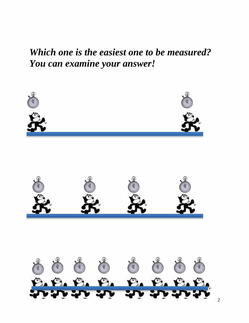
Which one is the easiest one to be measured?

You can examine your answer!

3

0. The Motion Detector and how it works

In the General Physics Lab we avoid this difficult measurment by stealing an idea found

in the natural world.

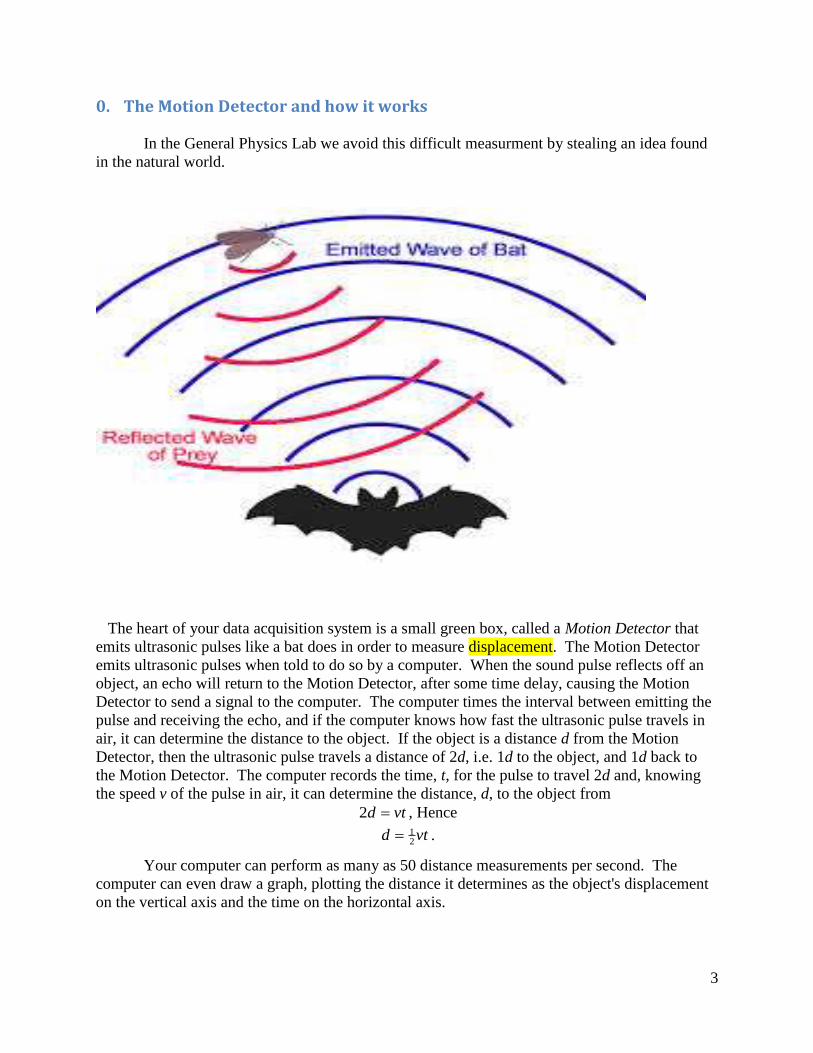
The heart of your data acquisition system is a small green box, called a Motion Detector that

emits ultrasonic pulses like a bat does in order to measure displacement. The Motion Detector

emits ultrasonic pulses when told to do so by a computer. When the sound pulse reflects off an

object, an echo will return to the Motion Detector, after some time delay, causing the Motion

Detector to send a signal to the computer. The computer times the interval between emitting the

pulse and receiving the echo, and if the computer knows how fast the ultrasonic pulse travels in

air, it can determine the distance to the object. If the object is a distance d from the Motion

Detector, then the ultrasonic pulse travels a distance of 2d, i.e. 1d to the object, and 1d back to

the Motion Detector. The computer records the time, t, for the pulse to travel 2d and, knowing

the speed v of the pulse in air, it can determine the distance, d, to the object from

, Hence

.

Your computer can perform as many as 50 distance measurements per second. The

computer can even draw a graph, plotting the distance it determines as the object's displacement

on the vertical axis and the time on the horizontal axis.

tvd 2

tvd21

4

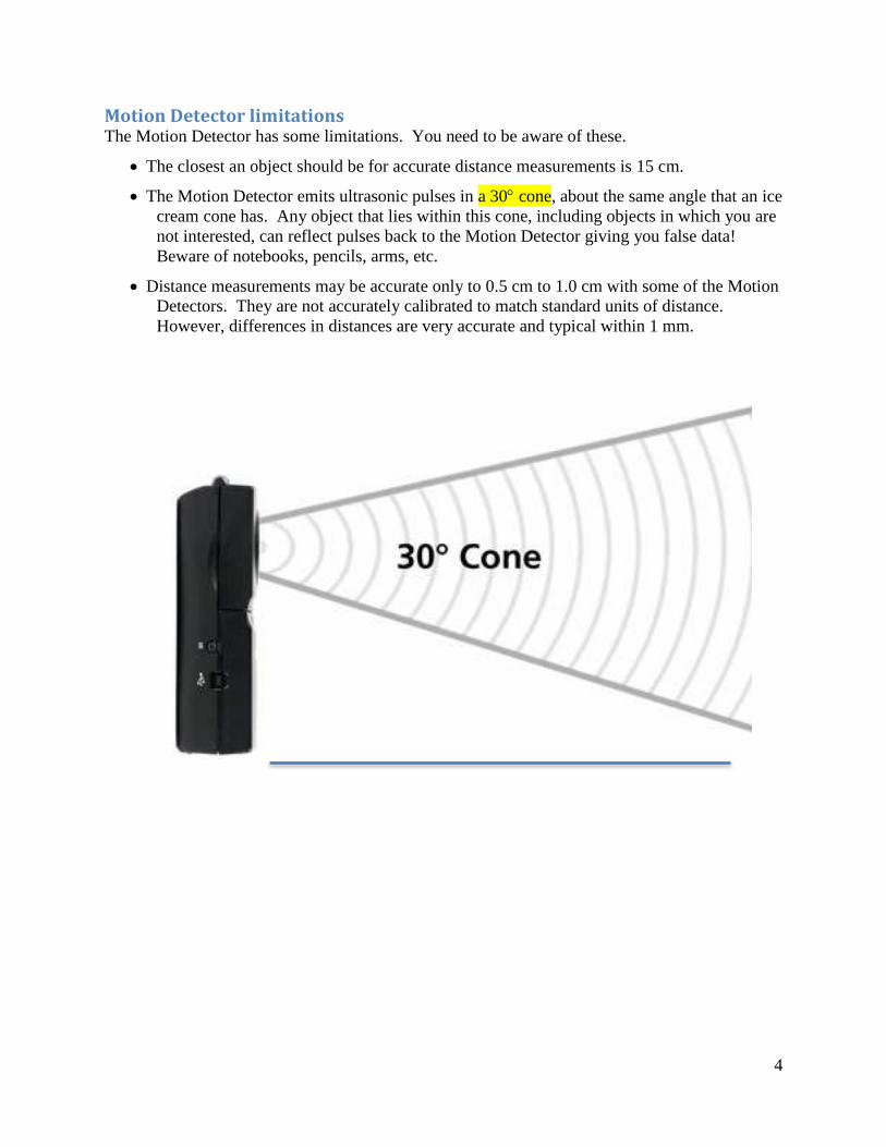
Motion Detector limitations The Motion Detector has some limitations. You need to be aware of these.

The closest an object should be for accurate distance measurements is 15 cm.

The Motion Detector emits ultrasonic pulses in a 30 cone, about the same angle that an ice

cream cone has. Any object that lies within this cone, including objects in which you are

not interested, can reflect pulses back to the Motion Detector giving you false data!

Beware of notebooks, pencils, arms, etc.

Distance measurements may be accurate only to 0.5 cm to 1.0 cm with some of the Motion

Detectors. They are not accurately calibrated to match standard units of distance.

However, differences in distances are very accurate and typical within 1 mm.

5

Materials:

Meter sticks

Two metal angle brackets

PC with LabQuest computer interface box for measuring instruments

Motion Sensor (also known as a "sonic ranger")

PASCO cart on aluminum tracks (activities 3-5)

Activity:

1. Use of meter stick to measure static positions

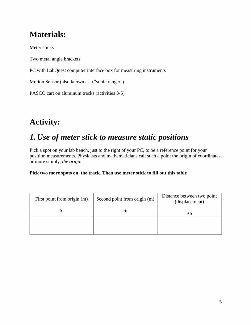
Pick a spot on your lab bench, just to the right of your PC, to be a reference point for your

position measurements. Physicists and mathematicians call such a point the origin of coordinates,

or more simply, the origin.

Pick two more spots on the track. Then use meter stick to fill out this table

First point from origin (m)

Si

Second point from origin (m)

Sf

Distance between two point

(displacement)

S

6

2. Use of sonic ranger to measure static positions

Now you will make your first use of the computerized measuring equipment.

Open PHY221 on the computer and then click on the Logger Pro 3.8.3 icon. If graphs of

position and velocity as a function of time do not appear, check that the Motion Detector

("sonic ranger") is plugged into DIG 1 of the Lab Quest interface box and Lab Quest is on.

Next, click on the green button labeled "Collect" near the top of the screen. When you hear a

clicking sound, move your hand around near the front of the sonic ranger.

2. Do you see a relationship between the position of your hand and the height of the red

line of the graph on the computer? What is the relationship?

Now you are ready to try some real quantitative measurements of position and displacement

using the sonic ranger. Set the sonic ranger at the spot you called your origin of coordinates, and

leave the meter stick aligned as you had it before. Place the angle bracket at the first position

from part 1, then click on the "Collect" button on the screen. After a few seconds, move the angle

bracket to the second position from part 1. (You can set your origin of coordinates to be zero

with the sonic ranger, by clicking on Experiment/Zero when the sonic ranger is looking at an

angle bracket set to reflect the signal from the sonic ranger sitting at your coordinate origin.)

From File menu click on PRINT to copy your graphs to the printer. Be careful to fill in all your

names so they will appear on the print. In what follows make appropriate annotations on the

printed copy as necessary.

3. What part of the graph corresponds to the angle bracket sitting at the first position?

What part of the graph corresponds to the angle bracket sitting at the second position?

Indicate your answers on the graph above.

4. Now read off the positions of the angle bracket at the two locations. For rough

measurements, you can just read the graph by eye. What are the two positions?

7

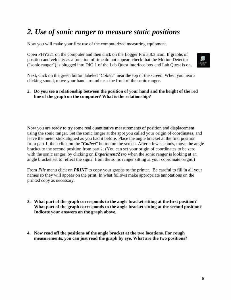
For more accurate results, bring up the measurement cursor. Turn it on by clicking on the button

labeled "x=?" on the toolbar near the top of the screen. You should see a vertical line that moves

across the graph as you move the mouse, and a little window near the top of the graph that

displays the value of the distance D corresponding to the time where you place the cursor.

First point from origin (m)

Si

Second point from origin (m)

Sf

Distance between two point

(displacement)

S

5. Comment on the similarities and differences between the position and displacement

measurement made with the sonic ranger, compared with the one made with just a

meter stick.

Does either displacement or position measurement depend on the choice of the origin of

coordinates?

8

3. Measurement of x(t) for a moving object using a

meter stick

Put one of the aluminum tracks on your lab bench and place a PASCO cart on it. Ensure that the

cart moves freely on the track.

Try a measurement of the position of the cart as a function of time x(t), as it moves freely down

the track (give it initial push and then let it go). Set up a meter stick alongside the track. Each

student in a team of three has a key role to play here. The Leader sets the cart in motion, and then

calls out one-second intervals using her watch. The Critic reads the position of the cart along the

meter stick at each second. The Scribe records the positions as they are called out. The Leader is

responsible for ensuring that the cart does not fall off the track (at least 3second).

Make a graph of position vs. time:

6. How well does this procedure work? Is it accurate? Could you track complicated

motions with such a procedure? Justify your answers.

9

4. Measurement of x(t) for a moving object using the

sonic ranger

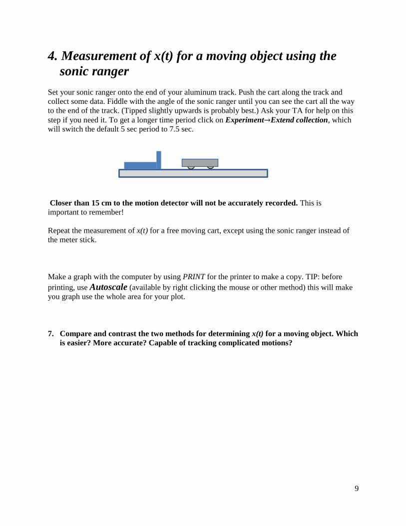
Set your sonic ranger onto the end of your aluminum track. Push the cart along the track and

collect some data. Fiddle with the angle of the sonic ranger until you can see the cart all the way

to the end of the track. (Tipped slightly upwards is probably best.) Ask your TA for help on this

step if you need it. To get a longer time period click on Experiment→Extend collection, which

will switch the default 5 sec period to 7.5 sec.

Closer than 15 cm to the motion detector will not be accurately recorded. This is

important to remember!

Repeat the measurement of x(t) for a free moving cart, except using the sonic ranger instead of

the meter stick.

Make a graph with the computer by using PRINT for the printer to make a copy. TIP: before

printing, use Autoscale (available by right clicking the mouse or other method) this will make

you graph use the whole area for your plot.

7. Compare and contrast the two methods for determining x(t) for a moving object. Which

is easier? More accurate? Capable of tracking complicated motions?

10

5. Average velocity

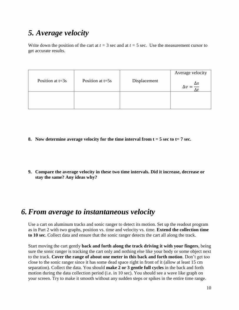
Write down the position of the cart at t = 3 sec and at t = 5 sec. Use the measurement cursor to

get accurate results.

Position at t=3s Position at t=5s Displacement

Average velocity

Δ𝑣 =Δ𝑠

Δ𝑡

8. Now determine average velocity for the time interval from t = 5 sec to t= 7 sec.

9. Compare the average velocity in these two time intervals. Did it increase, decrease or

stay the same? Any ideas why?

6. From average to instantaneous velocity

Use a cart on aluminum tracks and sonic ranger to detect its motion. Set up the readout program

as in Part 2 with two graphs, position vs. time and velocity vs. time. Extend the collection time

to 10 sec. Collect data and ensure that the sonic ranger detects the cart all along the track.

Start moving the cart gently back and forth along the track driving it with your fingers, being

sure the sonic ranger is tracking the cart only and nothing else like your body or some object next

to the track. Cover the range of about one meter in this back and forth motion. Don’t get too

close to the sonic ranger since it has some dead space right in front of it (allow at least 15 cm

separation). Collect the data. You should make 2 or 3 gentle full cycles in the back and forth

motion during the data collection period (i.e. in 10 sec). You should see a wave like graph on

your screen. Try to make it smooth without any sudden steps or spikes in the entire time range.

11

Once you are happy with the recorded result “Autoscale” the graphs then use PRINT to copy

your graph to the printer.

Pick up these following time moments on your graph (each time you are asked to pick a time

moment mark it on the printed graph).

A: middle point between the closest and the farthest distance from the sonic ranger while cart

moving away from the sonic ranger

tA= xA=

B: next time moment when the cart came back to the same position . Record the time and

position from the graph:

tB= xB=

Calculate average velocity for the AB time period:

vAB= xAB / tAB = (xB- xA)/(tB- tA) =

The cart was definitely moving in this time interval. Comment on the meaning of the value

of the average velocity you have just obtained.

C: time moment in between A and B when the cart was at the largest distance from the sonic

ranger.

tC= xC=

D: close to mid-time between A and C.

tD= xD=

Finally make time “E” to be as close as you can to time A (being still different from A).

tE= xE=

12

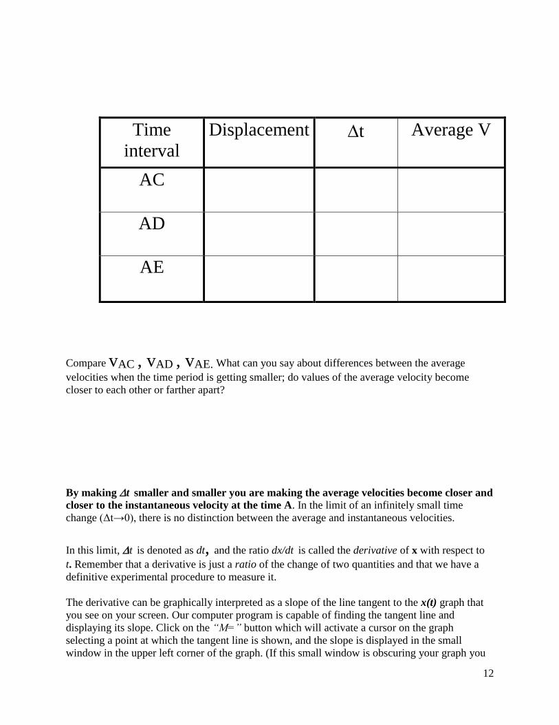
Time

interval

Displacement t Average V

AC

AD

AE

Compare vAC , vAD , vAE. What can you say about differences between the average

velocities when the time period is getting smaller; do values of the average velocity become

closer to each other or farther apart?

By making t smaller and smaller you are making the average velocities become closer and

closer to the instantaneous velocity at the time A. In the limit of an infinitely small time

change (Δt→0), there is no distinction between the average and instantaneous velocities.

In this limit, t is denoted as dt, and the ratio dx/dt is called the derivative of x with respect to

t. Remember that a derivative is just a ratio of the change of two quantities and that we have a

definitive experimental procedure to measure it.

The derivative can be graphically interpreted as a slope of the line tangent to the x(t) graph that

you see on your screen. Our computer program is capable of finding the tangent line and

displaying its slope. Click on the “M=” button which will activate a cursor on the graph

selecting a point at which the tangent line is shown, and the slope is displayed in the small

window in the upper left corner of the graph. (If this small window is obscuring your graph you

13

can reposition it by dragging it with the mouse). Position the cursor at the time moment A. Write

down the slope of the line, which gives you the instantaneous velocity at the time A:

vA= dx/dt = slope =

Compare the instantaneous velocity measured above with the average velocity vAE. Are they

close to each other?

7. Inspection of instantaneous velocity at various times

Using “M=” cursor determine and write done instantaneous velocity at the time moments A, C,

and B:

vA=

vC=

vB=

Comment on the value of instantaneous velocity at time C (that we defined as the point of the

farthest distance from the sonic ranger):

Comment on relative sign of instantaneous velocity at time A and B. What is the meaning of the

sign of velocity?

14

15

Pre-Lab Questions Print Your Name

______________________________________ Read the Introduction to this handout, and answer the following questions before you come to Physics Lab.

Write your answers directly on this page. When you enter the lab, tear off this page. Your TA will collect this at the

beginning of the session.

1. What does the Motion Detector do?

2. What goes wrong if an object gets too close to the Motion Detector?

3. How close is too close?

4. The Motion Detector works by (choose correct item) (a) timing radio waves, (b) radar, (c)

timing sound waves, (d) using visible light, (e) a meter stick.

5. How wide is the beam emitted by the Motion Detector?

6. What happens if you leave a notebook near the object the Motion Detector is monitoring?

7. The Motion detector uses the formula distance = ½vt. The usual formula for distance is

distance = vt. Why does the Motion Detector use a different formula?

8. About how accurate are the Motion Detectors?

9. Please solve for a.

sf = si + vit + ½at2