Pose-Space Subspace Dynamics

Hongyi Xu Jernej BarbicUniversity of Southern California

Figure 1: Hard-real-time soft tissue FEM dynamics compatible with standard character rigging. The input gorilla skeletal (60 DOFs)motion was obtained by retargeting the Kinect-captured motion to the gorilla character in real time. Our method produces physically basedFEM dynamics of the gorilla soft tissue. The simulator runs at fast simulation rates (750 simulation FPS, 16,297 tetrahedra, 15,744 triangles)and is suitable for applications in games and virtual reality. Speed is achieved using pose-dependent model reduction. We precomputeseparate reduced models at 4 representative gorilla poses. At runtime, simulation is performed in a time-varying basis that is obtained byinterpolating the precomputed bases to the current pose. Our method fits into the standard pose-space deformation (PSD) pipeline wherebyself-contact and skinning artifacts are resolved, by artists, in each pose and stored as pose-space deformation corrections, and interpolatedat runtime. Our subspace is aware of the contact constraints and prohibits dynamics that cause deeper penetrations.

Abstract

We enrich character animations with secondary soft-tissue FiniteElement Method (FEM) dynamics computed under arbitrary riggedor skeletal motion. Our method optionally incorporates pose-spacedeformation (PSD). It runs at milliseconds per frame for com-plex characters, and fits directly into standard character animationpipelines. Our simulation method does not require any skin datacapture; hence, it can be applied to humans, animals, and arbitrary(real-world or fictional) characters. In standard model reduction ofthree-dimensional nonlinear solid elastic models, one builds a re-duced model around a single pose, typically the rest configuration.We demonstrate how to perform multi-model reduction of Finite El-ement Method (FEM) nonlinear elasticity, where separate reducedmodels are precomputed around a representative set of object poses,and then combined at runtime into a single fast dynamic system, us-ing subspace interpolation. While time-varying reduction has beendemonstrated before for offline applications, our method is fast andsuitable for hard real-time applications in games and virtual reality.Our method supports self-contact, which we achieve by computinglinear modes and derivatives under contact constraints.

Keywords: physically based simulation, character rigging, pose-space, model reduction, FEM, secondary motion, real-time

Concepts: •Computing methodologies→ Physical simulation;

Permission to make digital or hard copies of all or part of this work for per-sonal or classroom use is granted without fee provided that copies are notmade or distributed for profit or commercial advantage and that copies bearthis notice and the full citation on the first page. Copyrights for componentsof this work owned by others than the author(s) must be honored. Abstract-ing with credit is permitted. To copy otherwise, or republish, to post onservers or to redistribute to lists, requires prior specific permission and/or afee. Request permissions from permissions@acm.org. c© 2016 Copyrightheld by the owner/author(s). Publication rights licensed to ACM.SIGGRAPH ’16 Technical Paper,, July 24 - 28, 2016, Anaheim, CA,ISBN: 978-1-4503-4279-7/16/07DOI: http://dx.doi.org/10.1145/2897824.2925916

1 Introduction

In computer animation practice, characters are typically animatedby first animating the skeleton or rig parameters, either by handor by using a data-driven technique (motion capture). The polyg-onal mesh of the character is then deformed kinematically, usinga rigging or skinning approach. In order to animate the bulging ofmuscles, correct the artifacts of linear blend skinning, or sculpt arbi-trary, pose-dependent modifications to standard skinning, it is com-mon to use the technique of pose-space deformation (PSD). In PSD,one sculpts pose-dependent corrections to rigging/skinning, andthen interpolates them to arbitrary poses using radial-basis func-tions. PSD is, however, a static technique: for a given pose, it al-ways returns the same shape. In this paper, we investigate how to in-corporate physically based simulation into rigging/skinning and/orPSD, to automatically produce secondary skin motion. We presenta method that has the following properties: (1) it runs at under 1-2msec per frame for complex models and is as such suitable for real-time applications in games and virtual reality, (2) it uses the FiniteElement Method (FEM) to give simulations a non-jiggly, “solid”look, (3) it works with an arbitrary skinning/rigging method, (4)supports character self-collisions, such as in the elbow and shoulderregions, and (5) it fits into standard computer animation pipelines.Our skin dynamics is driven by the inertial forces due to the skele-ton or rig-induced motion, or by gravity or other external forces.Our method uses physically based simulation and does not requirescanning skin data from real subjects. As such, it is suitable for car-toon characters, animals, fantasy creatures, in addition to humans.

Our technique works by combining the Finite Element Method withpose-dependent model reduction. Model reduction is a techniquewherein high-dimensional equations of motions are projected to asuitable, more manageable low-dimensional space. Model reduc-tion has been commonly employed in computer animation to ac-celerate physically based simulations. In standard model reduc-tion of three-dimensional nonlinear solid elastic models, however,one builds a reduced model around a single pose, typically therest configuration. Such a basis becomes inaccurate as the char-acter pose deviates from the rest configuration, due to the changinggeometric shape under skinning or rigging, and pose-dependent,artist-sculpted changes in character geometry and material proper-ties. Standard model reduction also suffers from non-locality of

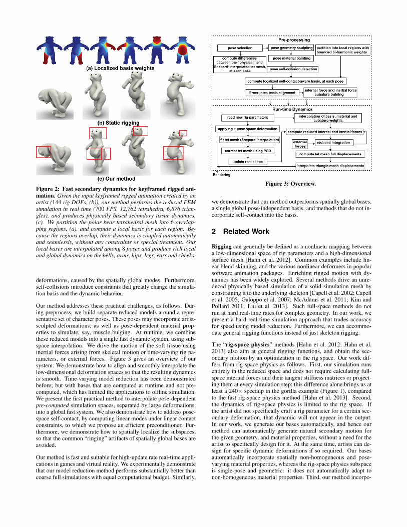
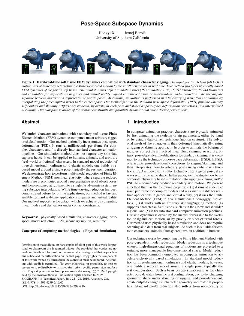
Figure 2: Fast secondary dynamics for keyframed rigged ani-mation. Given the input keyframed rigged animation created by anartist (144 rig DOFs, (b)), our method performs the reduced FEMsimulation in real time (700 FPS, 12,762 tetrahedra, 6,876 trian-gles), and produces physically based secondary tissue dynamics,(c). We partition the polar bear tetrahedral mesh into 6 overlap-ping regions, (a), and compute a local basis for each region. Be-cause the regions overlap, their dynamics is coupled automaticallyand seamlessly, without any constraints or special treatment. Ourlocal bases are interpolated among 8 poses and produce rich localand global dynamics on the belly, arms, hips, legs, ears and cheeks.

deformations, caused by the spatially global modes. Furthermore,self-collisions introduce constraints that greatly change the simula-tion basis and the dynamic behavior.

Our method addresses these practical challenges, as follows. Dur-ing preprocess, we build separate reduced models around a repre-sentative set of character poses. These poses may incorporate artist-sculpted deformations, as well as pose-dependent material prop-erties to simulate, say, muscle bulging. At runtime, we combinethese reduced models into a single fast dynamic system, using sub-space interpolation. We drive the motion of the soft tissue usinginertial forces arising from skeletal motion or time-varying rig pa-rameters, or external forces. Figure 3 gives an overview of oursystem. We demonstrate how to align and smoothly interpolate thelow-dimensional deformation spaces so that the resulting dynamicsis smooth. Time-varying model reduction has been demonstratedbefore; but with bases that are computed at runtime and not pre-computed, which has limited the applications to offline simulation.We present the first practical method to interpolate pose-dependentpre-computed simulation spaces, separated by large deformations,into a global fast system. We also demonstrate how to address pose-space self-contact, by computing linear modes under linear contactconstraints, to which we propose an efficient preconditioner. Fur-thermore, we demonstrate how to spatially localize the subspaces,so that the common “ringing” artifacts of spatially global bases areavoided.

Our method is fast and suitable for high-update rate real-time appli-cations in games and virtual reality. We experimentally demonstratethat our model reduction method performs substantially better thancoarse full simulations with equal computational budget. Similarly,

Figure 3: Overview.

we demonstrate that our method outperforms spatially global bases,a single global pose-independent basis, and methods that do not in-corporate self-contact into the basis.

2 Related Work

Rigging can generally be defined as a nonlinear mapping betweena low-dimensional space of rig parameters and a high-dimensionalsurface mesh [Hahn et al. 2012]. Common examples include lin-ear blend skinning, and the various nonlinear deformers in popularsoftware animation packages. Enriching rigged motion with dy-namics has been widely explored. Several methods drive an unre-duced physically based simulation of a solid simulation mesh byconstraining it to the underlying skeleton [Capell et al. 2002; Capellet al. 2005; Galoppo et al. 2007; McAdams et al. 2011; Kim andPollard 2011; Liu et al. 2013]. Such full-space methods do notrun at hard real-time rates for complex geometry. In our work, wepresent a hard real-time simulation approach that trades accuracyfor speed using model reduction. Furthermore, we can accommo-date general rigging functions instead of just skeleton rigging.

The “rig-space physics” methods [Hahn et al. 2012; Hahn et al.2013] also aim at general rigging functions, and obtain the sec-ondary motion by an optimization in the rig space. Our work dif-fers from rig-space physics as follows. First, our simulation runsentirely in the reduced space and does not require calculating full-space internal forces and their tangent stiffness matrices or project-ing them at every simulation step; this difference alone brings us atleast a 240× speedup in the gorilla example (Figure 1), comparedto the fast rig-space physics method [Hahn et al. 2013]. Second,the dynamics of rig-space physics is limited to the rig space. Ifthe artist did not specifically craft a rig parameter for a certain sec-ondary deformation, that dynamic will not appear in the output.In our work, we generate our bases automatically, and hence ourmethod can automatically generate natural secondary motion forthe given geometry, and material properties, without a need for theartist to specifically design for it. At the same time, artists can de-sign for specific dynamic deformations if so required. Our basesautomatically incorporate spatially non-homogeneous and pose-varying material properties, whereas the rig-space physics subspaceis single-pose and geometric: it does not automatically adapt tonon-homogeneous material properties. Third, our method incorpo-

rates a fast self-contact handling method, by baking the per-posecontact state into the per-pose basis.

Subspace methods have been popular in accelerating simulationsof deformable solids [James and Pai 2002; Hauser et al. 2003;Barbic and James 2005; An et al. 2008; Hildebrandt et al. 2012].While fast, it is not immediately obvious how to apply such meth-ods to character animation pipelines that typically use rigging orskinning. Model reduction has proven useful to increase perfor-mance for static pose-space deformation without dynamics [Kryet al. 2002], and for dynamic simulation [Galoppo et al. 2009; Hahnet al. 2014; Teng et al. 2015]. A common theme in these papersis to un-transform the simulation data with the skinning transfor-mation to the neutral character pose, and then model-reduce it.However, these prior methods evaluated reduced dynamics withrespect to the neutral pose of the character, which is inaccuratefor characters undergoing large deformations. Our pose-dependentbases, and the reduced elastic internal forces and stiffness matrices,are computed with respect to the geometry and material proper-ties of each pose, which substantially improves dynamics aroundposes that contain large deformations. Given several morph targets,Galoppo et al. [2009] constructed a single pose-independent (alsocalled pose-global) basis by performing PCA on the sets of basescomputed at the undeformed configuration, but with per-pose mate-rial properties and PSD corrections. However, for poses that differsignificantly from the undeformed configuration, bases computedat the undeformed pose will produce incorrect dynamics. Differentfrom them, we compute a separate basis at a set of selected poses.Because we never construct a pose-global basis, each of our per-pose bases can have a small dimension, enabling faster simulationrates. At runtime, we interpolate the precomputed bases to the run-time poses. Therefore, our simulator uses a smaller basis, whileobtaining more plausible dynamics.

High-quality skin simulations can be achieved using data-driven methods, combined with second-order auto-regressive mod-els [Pons-Moll et al. 2015]. However, such a method requires areal-life subject capture session, and is as such mostly limited tohumans. Our simulation method can be used to animate arbitrarycreatures, beyond humans. With our method, the animator can alsoeasily tweak the material properties of the tissue, and as such se-lectively adjust the dynamics at the various parts of the creature.Several simulation methods obtain the basis by performing PCAon full simulation data [Kry et al. 2002; Hahn et al. 2014; Tenget al. 2015]. We create pose-dependent bases automatically, withstandard modal analysis techniques, based on geometry and ma-terial properties only, and without any training data. To accom-modate large deformations, one can enrich the basis using modalderivatives [Barbic and James 2005], or linear transformations ofthe basis [von Tycowicz et al. 2013]. Our approach is agnostic tothe specific enrichment method; we choose linear modes and modalderivatives. For fast modal integration, radial basis interpolation ofcubic force polynomials for the St.Venant-Kirchoff material [Ga-loppo et al. 2009], or pose-space cubature interpolation of contactforces [Teng et al. 2014] have been studied. We demonstrate how toperform pose-space cubature interpolation of general hyperelasticnonlinear materials, with different geometry and materials at eachpose. We also demonstrate how to employ cubature to efficientlyevaluate the reduced inertial forces.

Our method modifies the simulation basis at runtime. Kim etal. [2009] proposed an online model reduction method which al-ternates between full and reduced simulation. Our approach alwaysuses reduced simulation, without the need for any runtime full sim-ulation, which makes it possible to run the simulation consistentlyat hard real-time rates. Temporally adaptive bases can also be con-structed by selecting a few basis vectors from a large precomputeddatabase [Hahn et al. 2014]. Their approach, however, requires the

evaluation and projection of full-space internal forces and stiffnessmatrices, which we can avoid. Furthermore, in order to avoid pop-ping, their method requires re-projecting the deformation at eachframe to a new basis. Our method creates the subspace by inter-polating aligned basis vectors, which requires no re-projection andtherefore avoid re-projection errors and loss of energy.

In the engineering community, interpolation between parameter-ized reduced-order models has been explored for aeroelasticity,thermal design and probabilistic analysis [Amsallem and Farhat2008; Degroote et al. 2010; Amsallem and Farhat 2011]. In thesemethods, the varying parameter is typically a flow constant, suchas the Mach number, whereas the structural deformations are smalland often linearized. In our work, we interpolate bases for geomet-ric shapes that have undergone large deformations. Different fromthese methods outside of computer graphics, we demonstrate howto construct a system that runs at hard real-time rates for complexthree-dimensional geometry undergoing large deformations.

Teng et al. [2014] computed self-contact forces in the subspace withpose-space cubature, by exploiting contact coherence for articu-lated bodies. Similarly, we detect self-contact at example poses, butthen bake the contact information into the construction of our pose-dependent bases. This avoids the need for run-time self-collisiondetection and resolution, trading accuracy for performance for hardreal-time applications. We also demonstrate how to support local-ized deformations using spatially localized basis functions. Localsubspace deformations can be accommodated with the use of ana-lytic Boussinesq solutions [Harmon and Zorin 2013], bi-harmonicweights [Jacobson et al. 2011], discrete Laplacian [Wang et al.2015], sparse matrix decomposition of animation sequences [Neu-mann et al. 2013], or domain decomposition [Barbic and Zhao2011; Kim and James 2012; Yang et al. 2013]. Huang et al. [2012]trained spatially-local skinning deformation mappings in the lo-cal pose space. In contrast to prior work, our localized deforma-tions are designed for physical simulation involving large defor-mations induced by a character rig, and are free of seaming arti-facts. We construct our localized bases by letting the user spec-ify a few points to denote individual regions, upon which a scalar“region function” is computed for each region, using bounded bi-harmonic weights [Jacobson et al. 2011]. Different from [Jacobsonet al. 2011] who used bi-harmonic functions directly as the defor-mation subspace for static shape editing, we only use them to defineoverlapping regions for model reduction, and simulate real-time dy-namics.

3 Background: Pose-Space Deformation

In our work, we add physically based secondary motion effects, inreal-time, to triangle mesh animations obtained using any charac-ter rigging process. In order to do so, we will employ a simulationtetrahedral mesh. We denote all quantities y referring to the trian-gle and tetrahedral meshes as y and y, respectively. The input toour method is an undeformed (also called neutral) triangle meshΓ ∈ R3n with n vertices with positions X ∈ R3n, alongside with anarbitrary rigging function Φ(p, X). Here, p ∈ Rs is the rig parame-ter which defines the specific pose. The rig function Φ(p, X) ∈R3n

gives the rig-deformed vertex positions; these positions are stati-cally determined by p, devoid of any dynamics. Note that the posep may correspond to the joint angles of the character, but it canalso be more general; e.g., sliders in a rigging deformer, or evenany more abstract space. Our general formulation for Φ incorpo-rates elaborate character “production” rigs, nonlinear deformers,skeleton-based methods (linear blend skinning, dual quaternions),and blend-shape animations. In our system, the rigging function Φ

is treated as a black-box, and we do not require its explicit formula;we only need the ability to evaluate Φ(p, X) for an arbitrary p and

X . This allows us to use our method with, say, standard animationpackages such as Autodesk Maya.

Pose-space Deformation is a method that combines skeletonsubspace deformation (SSD) [Magnenat-Thalmann et al. 1988]with artist-corrected pose shapes [Lewis et al. 2000]. Given a set oftriangle mesh poses Si corresponding to poses pi, for i = 1, . . . ,m,typically obtained directly by skinning or rigging, the artist pro-vides corrections δi ∈R3n that, for example, undo a candy wrappereffect or improve volume preservation. We can then incorporatethese correction into the rig, by redefining it

Φ(p, X) → Φ(p, X)+ δ (p). (1)

The nonlinear deformation correction δ (p) can be obtained viascattered-data interpolation using Radial Basis Functions (RBF) inthe pose-space as

δ (p) =m

∑i=1

wi(p)δi, for wi(p) =m

∑j=1

wi jφ(‖p− p j‖), (2)

where wi(p) ∈ R, i = 1, . . . ,m, are the normalized interpolationweights, wi j ∈ R are the RBF-trained weights so that wi(p j) is 1when i = j and 0 otherwise, and φ is the RBF kernel function. Inour system, we employ the globally supported commonly used bi-harmonic RBF kernel φ(r) = r, considering the sparsity of the ex-ample poses [Carr et al. 2001]. Note that in principle, a distinctionin notation should be made between the original rig function, andthe rig function that incorporates the PSD corrections. In our paper,we will hereforth simply use Φ to denote the PSD-corrected rig, be-cause we never need to reference the original rig again. Our methodworks equally well even if there is no PSD correction. Because Xis constant, we will often drop X and simply write Φ(p).

4 Pose-Space Dynamics

How can one define meaningful physically-based dynamics for therigging function Φ? We assume that the trajectory p = p(t) is givenexternally, as our input. This is compatible with the usual com-puter animation pipelines, as p(t) can be obtained in any standardway: motion capture, procedural animation, inverse kinematics,etc. Therefore, in departure to prior work on rig-space physics,we chose not to modify p or evolve p according to an ODE. In-stead, we treat each configuration p as if it was a new rest config-uration of the object. The justification for this decision is that instatic (non-dynamic) PSD, a pose p uniquely defines the shape: ifp is kept constant, the shape in static PSD never changes and can assuch be seen as the rest shape corresponding to p. A similar viewhas been proposed by Liu et al. [2013], who used it for unreducedFEM simulation and control, limited to linear blend skinning andthe co-rotational material. As p= p(t) evolves over time, the objectundergoes a trajectory of rest configurations. For each p, we thensimulate dynamics on top of this time-varying rest pose. Note thatour dynamic PSD supports, using pose-space interpolation, effectssuch as materials stiffening in specific poses due to a large strain,or due to activation (muscles). We can simulate any physical force,such as gravity, collision forces or user forces. Additionally, the dy-namics are driven by the inertial (also called “system”, “fictitious”,or “d’Alembert”) forces, arising due to the changing rig parameterp. Inertial forces are responsible for most of our dynamics, such asthe tissue overshooting when the character stops, or deformationsunder Coriolis forces due to bone motion. The output of our methodis an animation of Γ that is driven by p = p(t), but is enriched withphysically-based secondary motion.

4.1 Pose-Space Tetrahedral Mesh

Our secondary motion originates from a pose-aware model-reducedFEM simulation of the tetrahedral mesh Γ ∈ R3n. During pre-process, we compute Γ by meshing the space enclosed by Γ, in theneutral configuration. Our method accommodates arbitrary, non-manifold triangular geometry Γ, using signed distance field mesh-ing [Xu and Barbic 2014]. The input rig function Φ is definedon the triangle mesh Γ, whereas we run physically-based simula-tions on the tetrahedral mesh Γ. Therefore, we need to define therig function Φ on the tetrahedral mesh. For each tet mesh vertex i,we perform this by interpolating the displacements of the nearest ktriangle mesh vertices (we use k = 4 in our method), using Shepard“inverse-distance” weights [Barnhill et al. 1983]. The interpolationweights are determined during the pre-process, in the neutral con-figuration. Such a method may produce a non-smooth deformationof Γ, when the vertex distribution of Γ is non-uniform. Therefore,in spirit of PSD, for each pose pi, we first compute a “physical”well-fitted tet mesh, using optimization [Barbic et al. 2009]

Φ(pi) = argminx

(‖Ax− Φ(pi)‖2

M + γE(x)). (3)

Here, A is the sparse barycentric interpolation matrix between Γ andΓ, determined in the neutral pose, E(x) is the elastic strain energyfor tet mesh vertex positions x with respect to the neutral configu-ration, and γ > 0 is a regularization constant. We store the differ-ence between the Shepard-interpolated mesh and Φ(pi) as correc-tions δ = {δ1,δ2, . . . ,δm}, at each pose. At run time, we correctthe Shepard-interpolated tet mesh with a PSD-interpolated correc-tion δ (p) = w(p)δ ∈ R3n. We note that the “rig-space physics”method [Hahn et al. 2013] addresses a similar technical issue bytraining weights relating displacements of surface simulation ver-tices to the interior vertices, using static simulation. While sucha method could be used to further improve the fit, the PSD schemeabove is very fast, and avoids the need for a weight training process.

4.2 Equations of Motion

Our dynamics is layered on top of the triangle mesh driven by therig parameter p. At any frame, we treat the current rigged meshΦ(p) as the rest shape. The dynamic deformation u ∈ R3n thengives the displacements away from this rest shape, in world coordi-nates. We write the equations of motion for the tetrahedral mesh as

M(p)u+Du+ fint(Φ(p),u

)= fext + finert, (4)

where M(p) ∈ R3n×3n is the mass matrix, D ∈ R3n×3n is thedamping matrix, fint(x,u) ∈ R3n is the internal force under therest shape x and displacements u away from x, fext ∈ R3n arethe external forces and finert ∈ R3n are the inertial forces causedby the motion p = p(t). We use the Rayleigh damping modelD = αM + βK(Φ(p),u), where K(Φ(p),u) ∈ R3n is the tangentstiffness matrix with respect to the current rest shape. Vector ugives the displacements relative to Φ(p), expressed in the world-coordinate system. We add the inertial force finert to model theeffect of the changing rig parameter p onto the deformation u. Con-sider a sequence of tet mesh rest poses x(p), under a time-varying p.Then, any location in the material, at any time t, undergoes a world-coordinate acceleration x(p) with respect to the world-coordinatesystem, simply because of the rig-induced motion. Therefore, fromthe point of view of a non-inertial coordinate system attached to asmall volume dV in the material, the material experiences an iner-tial force−ρ x(p)dV, where ρ is mass density. The inertial force onthe tet mesh vertices equals finert =−Ma(p) =−Md2x(p)/dt2. Weshow how to efficiently evaluate finert in Section 5.4. We computethe final deformed position of the triangle mesh Γ as Φ(p)+Au, as

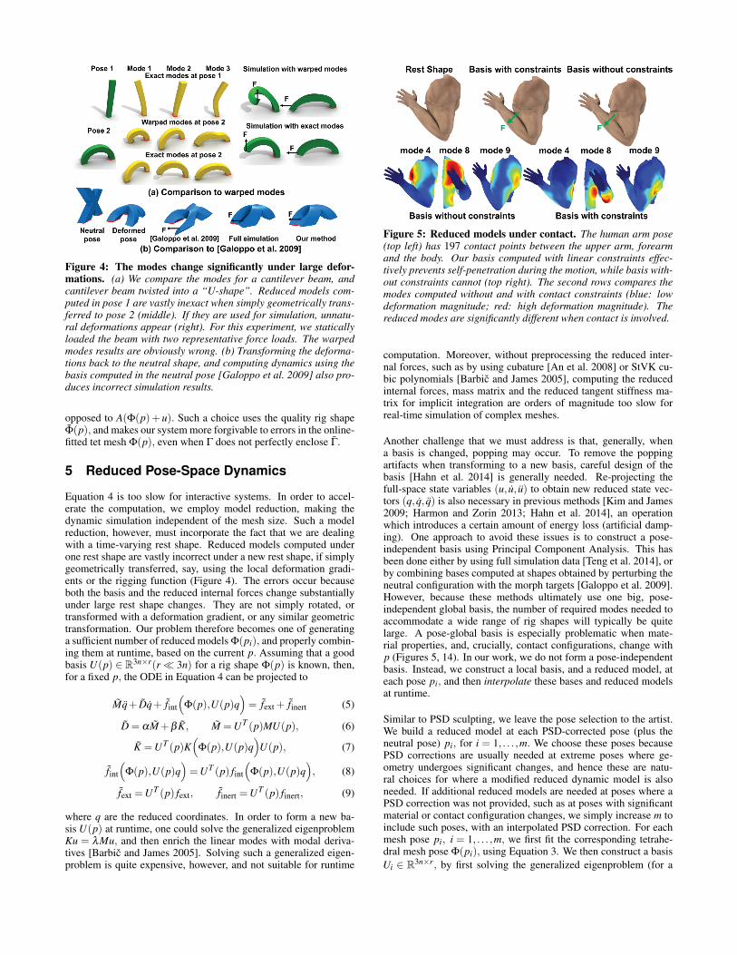
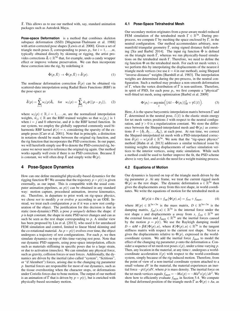
Figure 4: The modes change significantly under large defor-mations. (a) We compare the modes for a cantilever beam, andcantilever beam twisted into a “U-shape”. Reduced models com-puted in pose 1 are vastly inexact when simply geometrically trans-ferred to pose 2 (middle). If they are used for simulation, unnatu-ral deformations appear (right). For this experiment, we staticallyloaded the beam with two representative force loads. The warpedmodes results are obviously wrong. (b) Transforming the deforma-tions back to the neutral shape, and computing dynamics using thebasis computed in the neutral pose [Galoppo et al. 2009] also pro-duces incorrect simulation results.

opposed to A(Φ(p)+ u). Such a choice uses the quality rig shapeΦ(p), and makes our system more forgivable to errors in the online-fitted tet mesh Φ(p), even when Γ does not perfectly enclose Γ.

5 Reduced Pose-Space Dynamics

Equation 4 is too slow for interactive systems. In order to accel-erate the computation, we employ model reduction, making thedynamic simulation independent of the mesh size. Such a modelreduction, however, must incorporate the fact that we are dealingwith a time-varying rest shape. Reduced models computed underone rest shape are vastly incorrect under a new rest shape, if simplygeometrically transferred, say, using the local deformation gradi-ents or the rigging function (Figure 4). The errors occur becauseboth the basis and the reduced internal forces change substantiallyunder large rest shape changes. They are not simply rotated, ortransformed with a deformation gradient, or any similar geometrictransformation. Our problem therefore becomes one of generatinga sufficient number of reduced models Φ(pi), and properly combin-ing them at runtime, based on the current p. Assuming that a goodbasis U(p) ∈ R3n×r(r� 3n) for a rig shape Φ(p) is known, then,for a fixed p, the ODE in Equation 4 can be projected to

Mq+ Dq+ fint

(Φ(p),U(p)q

)= fext + finert (5)

D = αM+β K, M =UT (p)MU(p), (6)

K =UT (p)K(

Φ(p),U(p)q)

U(p), (7)

fint

(Φ(p),U(p)q

)=UT (p) fint

(Φ(p),U(p)q

), (8)

fext =UT (p) fext, finert =UT (p) finert, (9)

where q are the reduced coordinates. In order to form a new ba-sis U(p) at runtime, one could solve the generalized eigenproblemKu = λMu, and then enrich the linear modes with modal deriva-tives [Barbic and James 2005]. Solving such a generalized eigen-problem is quite expensive, however, and not suitable for runtime

Figure 5: Reduced models under contact. The human arm pose(top left) has 197 contact points between the upper arm, forearmand the body. Our basis computed with linear constraints effec-tively prevents self-penetration during the motion, while basis with-out constraints cannot (top right). The second rows compares themodes computed without and with contact constraints (blue: lowdeformation magnitude; red: high deformation magnitude). Thereduced modes are significantly different when contact is involved.

computation. Moreover, without preprocessing the reduced inter-nal forces, such as by using cubature [An et al. 2008] or StVK cu-bic polynomials [Barbic and James 2005], computing the reducedinternal forces, mass matrix and the reduced tangent stiffness ma-trix for implicit integration are orders of magnitude too slow forreal-time simulation of complex meshes.

Another challenge that we must address is that, generally, whena basis is changed, popping may occur. To remove the poppingartifacts when transforming to a new basis, careful design of thebasis [Hahn et al. 2014] is generally needed. Re-projecting thefull-space state variables (u, u, u) to obtain new reduced state vec-tors (q, q, q) is also necessary in previous methods [Kim and James2009; Harmon and Zorin 2013; Hahn et al. 2014], an operationwhich introduces a certain amount of energy loss (artificial damp-ing). One approach to avoid these issues is to construct a pose-independent basis using Principal Component Analysis. This hasbeen done either by using full simulation data [Teng et al. 2014], orby combining bases computed at shapes obtained by perturbing theneutral configuration with the morph targets [Galoppo et al. 2009].However, because these methods ultimately use one big, pose-independent global basis, the number of required modes needed toaccommodate a wide range of rig shapes will typically be quitelarge. A pose-global basis is especially problematic when mate-rial properties, and, crucially, contact configurations, change withp (Figures 5, 14). In our work, we do not form a pose-independentbasis. Instead, we construct a local basis, and a reduced model, ateach pose pi, and then interpolate these bases and reduced modelsat runtime.

Similar to PSD sculpting, we leave the pose selection to the artist.We build a reduced model at each PSD-corrected pose (plus theneutral pose) pi, for i = 1, . . . ,m. We choose these poses becausePSD corrections are usually needed at extreme poses where ge-ometry undergoes significant changes, and hence these are natu-ral choices for where a modified reduced dynamic model is alsoneeded. If additional reduced models are needed at poses where aPSD correction was not provided, such as at poses with significantmaterial or contact configuration changes, we simply increase m toinclude such poses, with an interpolated PSD correction. For eachmesh pose pi, i = 1, . . . ,m, we first fit the corresponding tetrahe-dral mesh pose Φ(pi), using Equation 3. We then construct a basisUi ∈ R3n×r, by first solving the generalized eigenproblem (for a

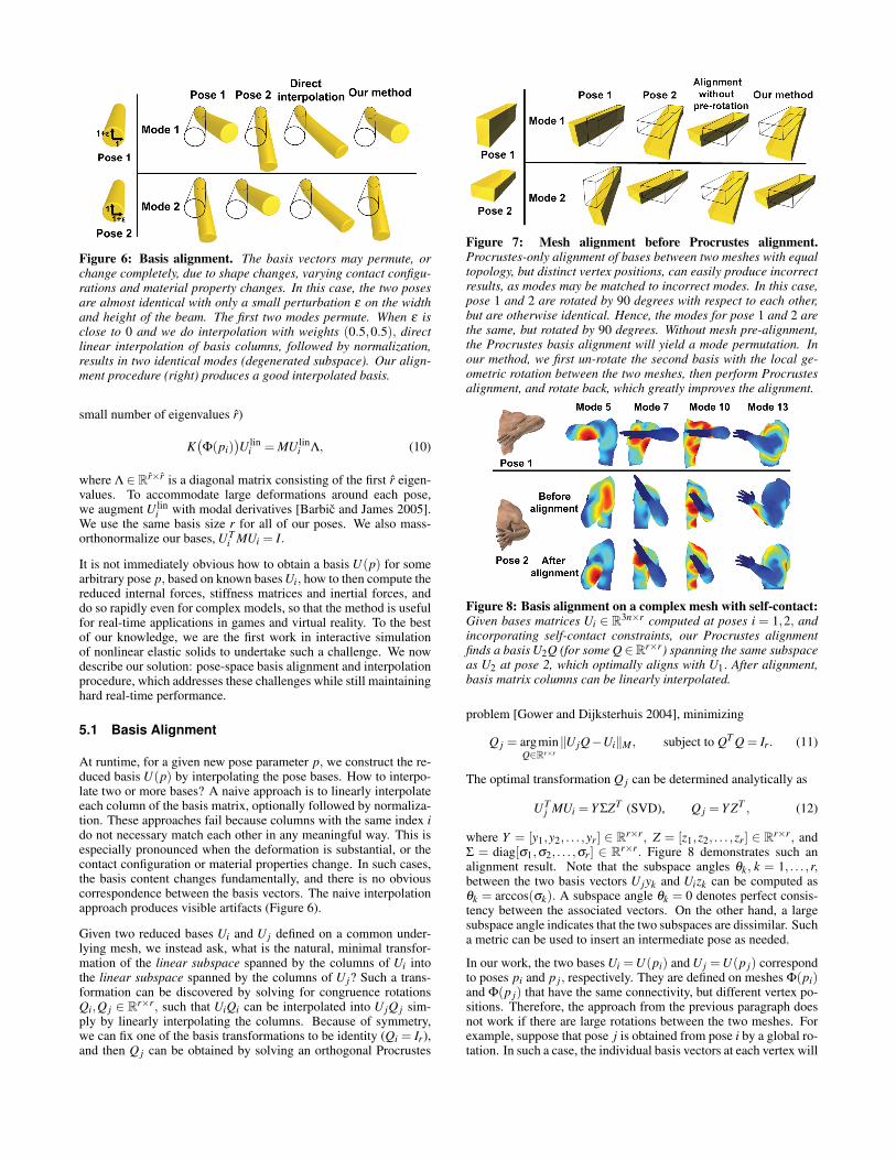
Figure 6: Basis alignment. The basis vectors may permute, orchange completely, due to shape changes, varying contact configu-rations and material property changes. In this case, the two posesare almost identical with only a small perturbation ε on the widthand height of the beam. The first two modes permute. When ε isclose to 0 and we do interpolation with weights (0.5,0.5), directlinear interpolation of basis columns, followed by normalization,results in two identical modes (degenerated subspace). Our align-ment procedure (right) produces a good interpolated basis.

small number of eigenvalues r)

K(Φ(pi)

)U lin

i = MU lini Λ, (10)

where Λ ∈ Rr×r is a diagonal matrix consisting of the first r eigen-values. To accommodate large deformations around each pose,we augment U lin

i with modal derivatives [Barbic and James 2005].We use the same basis size r for all of our poses. We also mass-orthonormalize our bases, UT

i MUi = I.

It is not immediately obvious how to obtain a basis U(p) for somearbitrary pose p, based on known bases Ui, how to then compute thereduced internal forces, stiffness matrices and inertial forces, anddo so rapidly even for complex models, so that the method is usefulfor real-time applications in games and virtual reality. To the bestof our knowledge, we are the first work in interactive simulationof nonlinear elastic solids to undertake such a challenge. We nowdescribe our solution: pose-space basis alignment and interpolationprocedure, which addresses these challenges while still maintaininghard real-time performance.

5.1 Basis Alignment

At runtime, for a given new pose parameter p, we construct the re-duced basis U(p) by interpolating the pose bases. How to interpo-late two or more bases? A naive approach is to linearly interpolateeach column of the basis matrix, optionally followed by normaliza-tion. These approaches fail because columns with the same index ido not necessary match each other in any meaningful way. This isespecially pronounced when the deformation is substantial, or thecontact configuration or material properties change. In such cases,the basis content changes fundamentally, and there is no obviouscorrespondence between the basis vectors. The naive interpolationapproach produces visible artifacts (Figure 6).

Given two reduced bases Ui and U j defined on a common under-lying mesh, we instead ask, what is the natural, minimal transfor-mation of the linear subspace spanned by the columns of Ui intothe linear subspace spanned by the columns of U j? Such a trans-formation can be discovered by solving for congruence rotationsQi,Q j ∈ Rr×r, such that UiQi can be interpolated into U jQ j sim-ply by linearly interpolating the columns. Because of symmetry,we can fix one of the basis transformations to be identity (Qi = Ir),and then Q j can be obtained by solving an orthogonal Procrustes

Figure 7: Mesh alignment before Procrustes alignment.Procrustes-only alignment of bases between two meshes with equaltopology, but distinct vertex positions, can easily produce incorrectresults, as modes may be matched to incorrect modes. In this case,pose 1 and 2 are rotated by 90 degrees with respect to each other,but are otherwise identical. Hence, the modes for pose 1 and 2 arethe same, but rotated by 90 degrees. Without mesh pre-alignment,the Procrustes basis alignment will yield a mode permutation. Inour method, we first un-rotate the second basis with the local ge-ometric rotation between the two meshes, then perform Procrustesalignment, and rotate back, which greatly improves the alignment.

Figure 8: Basis alignment on a complex mesh with self-contact:Given bases matrices Ui ∈ R3n×r computed at poses i = 1,2, andincorporating self-contact constraints, our Procrustes alignmentfinds a basis U2Q (for some Q∈Rr×r) spanning the same subspaceas U2 at pose 2, which optimally aligns with U1. After alignment,basis matrix columns can be linearly interpolated.

problem [Gower and Dijksterhuis 2004], minimizing

Q j = argminQ∈Rr×r

‖U jQ−Ui‖M , subject to QT Q = Ir. (11)

The optimal transformation Q j can be determined analytically as

UTj MUi = Y ΣZT (SVD), Q j = Y ZT , (12)

where Y = [y1,y2, . . . ,yr] ∈ Rr×r, Z = [z1,z2, . . . ,zr] ∈ Rr×r, andΣ = diag[σ1,σ2, . . . ,σr] ∈ Rr×r. Figure 8 demonstrates such analignment result. Note that the subspace angles θk, k = 1, . . . ,r,between the two basis vectors U jyk and Uizk can be computed asθk = arccos(σk). A subspace angle θk = 0 denotes perfect consis-tency between the associated vectors. On the other hand, a largesubspace angle indicates that the two subspaces are dissimilar. Sucha metric can be used to insert an intermediate pose as needed.

In our work, the two bases Ui =U(pi) and U j =U(p j) correspondto poses pi and p j, respectively. They are defined on meshes Φ(pi)and Φ(p j) that have the same connectivity, but different vertex po-sitions. Therefore, the approach from the previous paragraph doesnot work if there are large rotations between the two meshes. Forexample, suppose that pose j is obtained from pose i by a global ro-tation. In such a case, the individual basis vectors at each vertex will

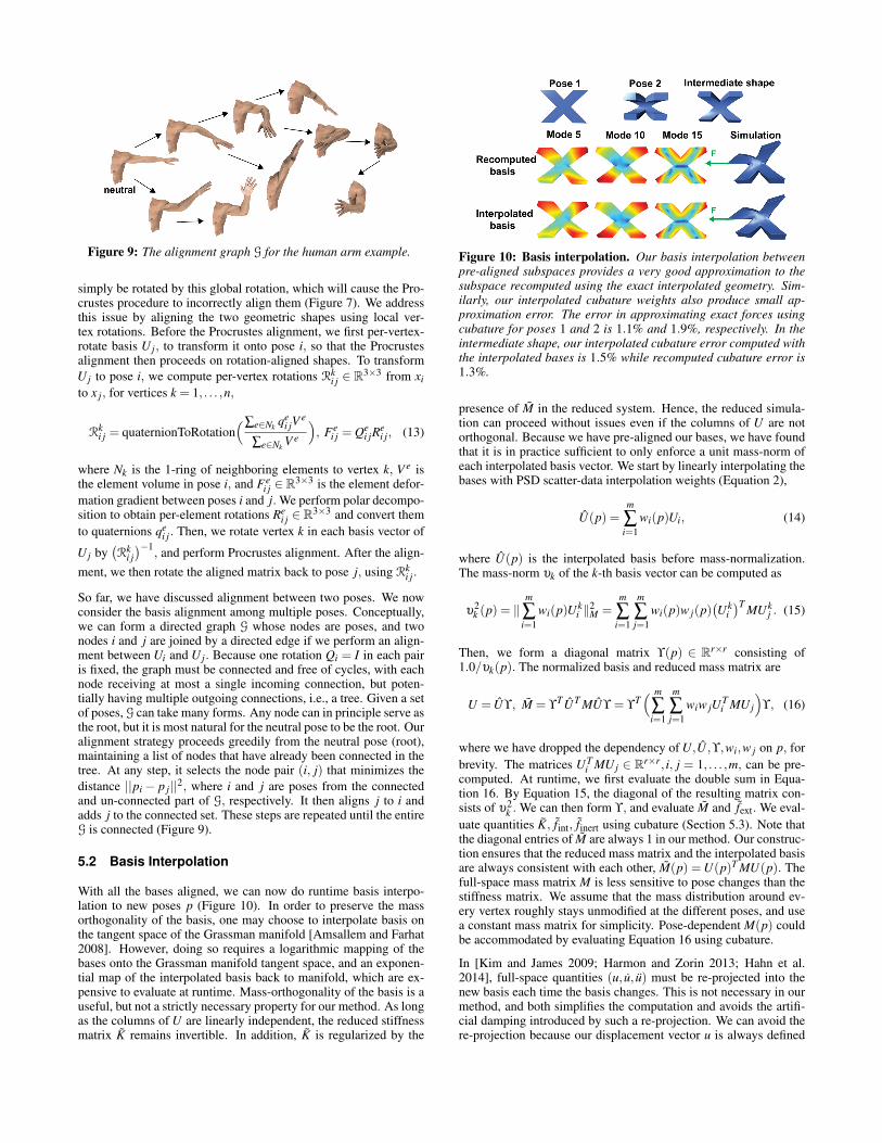
Figure 9: The alignment graph G for the human arm example.

simply be rotated by this global rotation, which will cause the Pro-crustes procedure to incorrectly align them (Figure 7). We addressthis issue by aligning the two geometric shapes using local ver-tex rotations. Before the Procrustes alignment, we first per-vertex-rotate basis U j, to transform it onto pose i, so that the Procrustesalignment then proceeds on rotation-aligned shapes. To transformU j to pose i, we compute per-vertex rotations Rk

i j ∈ R3×3 from xito x j, for vertices k = 1, . . . ,n,

Rki j = quaternionToRotation

(∑e∈Nkqe

i jVe

∑e∈NkV e

), Fe

i j = Qei jR

ei j, (13)

where Nk is the 1-ring of neighboring elements to vertex k, V e isthe element volume in pose i, and Fe

i j ∈ R3×3 is the element defor-mation gradient between poses i and j. We perform polar decompo-sition to obtain per-element rotations Re

i j ∈ R3×3 and convert themto quaternions qe

i j. Then, we rotate vertex k in each basis vector of

U j by(Rk

i j)−1

, and perform Procrustes alignment. After the align-ment, we then rotate the aligned matrix back to pose j, using Rk

i j.

So far, we have discussed alignment between two poses. We nowconsider the basis alignment among multiple poses. Conceptually,we can form a directed graph G whose nodes are poses, and twonodes i and j are joined by a directed edge if we perform an align-ment between Ui and U j. Because one rotation Qi = I in each pairis fixed, the graph must be connected and free of cycles, with eachnode receiving at most a single incoming connection, but poten-tially having multiple outgoing connections, i.e., a tree. Given a setof poses, G can take many forms. Any node can in principle serve asthe root, but it is most natural for the neutral pose to be the root. Ouralignment strategy proceeds greedily from the neutral pose (root),maintaining a list of nodes that have already been connected in thetree. At any step, it selects the node pair (i, j) that minimizes thedistance ||pi− p j||2, where i and j are poses from the connectedand un-connected part of G, respectively. It then aligns j to i andadds j to the connected set. These steps are repeated until the entireG is connected (Figure 9).

5.2 Basis Interpolation

With all the bases aligned, we can now do runtime basis interpo-lation to new poses p (Figure 10). In order to preserve the massorthogonality of the basis, one may choose to interpolate basis onthe tangent space of the Grassman manifold [Amsallem and Farhat2008]. However, doing so requires a logarithmic mapping of thebases onto the Grassman manifold tangent space, and an exponen-tial map of the interpolated basis back to manifold, which are ex-pensive to evaluate at runtime. Mass-orthogonality of the basis is auseful, but not a strictly necessary property for our method. As longas the columns of U are linearly independent, the reduced stiffnessmatrix K remains invertible. In addition, K is regularized by the

Figure 10: Basis interpolation. Our basis interpolation betweenpre-aligned subspaces provides a very good approximation to thesubspace recomputed using the exact interpolated geometry. Sim-ilarly, our interpolated cubature weights also produce small ap-proximation error. The error in approximating exact forces usingcubature for poses 1 and 2 is 1.1% and 1.9%, respectively. In theintermediate shape, our interpolated cubature error computed withthe interpolated bases is 1.5% while recomputed cubature error is1.3%.

presence of M in the reduced system. Hence, the reduced simula-tion can proceed without issues even if the columns of U are notorthogonal. Because we have pre-aligned our bases, we have foundthat it is in practice sufficient to only enforce a unit mass-norm ofeach interpolated basis vector. We start by linearly interpolating thebases with PSD scatter-data interpolation weights (Equation 2),

U(p) =m

∑i=1

wi(p)Ui, (14)

where U(p) is the interpolated basis before mass-normalization.The mass-norm υk of the k-th basis vector can be computed as

υ2k (p) = ‖

m

∑i=1

wi(p)Uki ‖2

M =m

∑i=1

m

∑j=1

wi(p)w j(p)(Uk

i)T MUk

j . (15)

Then, we form a diagonal matrix ϒ(p) ∈ Rr×r consisting of1.0/υk(p). The normalized basis and reduced mass matrix are

U = Uϒ, M = ϒTUT MUϒ = ϒ

T( m

∑i=1

m

∑j=1

wiw jUTi MU j

)ϒ, (16)

where we have dropped the dependency of U,U ,ϒ,wi,w j on p, forbrevity. The matrices UT

i MU j ∈ Rr×r, i, j = 1, . . . ,m, can be pre-computed. At runtime, we first evaluate the double sum in Equa-tion 16. By Equation 15, the diagonal of the resulting matrix con-sists of υ2

k . We can then form ϒ, and evaluate M and fext. We eval-uate quantities K, fint, finert using cubature (Section 5.3). Note thatthe diagonal entries of M are always 1 in our method. Our construc-tion ensures that the reduced mass matrix and the interpolated basisare always consistent with each other, M(p) =U(p)T MU(p). Thefull-space mass matrix M is less sensitive to pose changes than thestiffness matrix. We assume that the mass distribution around ev-ery vertex roughly stays unmodified at the different poses, and usea constant mass matrix for simplicity. Pose-dependent M(p) couldbe accommodated by evaluating Equation 16 using cubature.

In [Kim and James 2009; Harmon and Zorin 2013; Hahn et al.2014], full-space quantities (u, u, u) must be re-projected into thenew basis each time the basis changes. This is not necessary in ourmethod, and both simplifies the computation and avoids the artifi-cial damping introduced by such a re-projection. We can avoid there-projection because our displacement vector u is always defined

with respect to the current pose p. Similarly to how the rest shapesare morphed via the rig Φ(p), our basis interpolation can be seen asmorphing displacements (away from the rigged shape), as p varies.The basis U(p) defines the current local coordinates at each vertexthat interpret the meaning of q, and updating the pose p is equiv-alent to transforming this “local coordinate system”. Furthermore,the bases are pre-aligned and thus it is not necessary to remap thereduced quantities. We mass-normalize the basis and thus magni-tudes of the displacements vary smoothly, free of popping artifacts.

5.3 Pose-Space Cubature for Elasticity

We now describe how we quickly evaluate the reduced inter-nal forces fint(Φ(p),U(p)q) and reduced tangent stiffness matrixK(Φ(p),U(p)q), for general nonlinear material, under the interpo-lated basis U(p), for arbitrary p and q. For the linear StVK material,Galoppo [2009] proposed computing these quantities by the inter-polation of cubic polynomial coefficients associated with each pose.We introduce pose-space cubature to simulate arbitrary, nonlinearmaterials, similar in spirit to [An et al. 2008; Teng et al. 2014], butfor multi-pose reduced elasticity.

For each pose pi, we determine a cubature element set Ci, and thecorresponding cubature weights vi ∈ Rci , where ci = |Ci|. At run-time, we then linearly interpolate the cubature weights to each posep, using PSD weights. In each pose pi, we generate T random cu-bature samples, q(i,k), k = 1, . . . ,T. The samples are obtained byrandomly sampling a Gaussian distribution for each mode, withstandard deviations proportional to the inverse of the modes stiff-ness [An et al. 2008]. Independent cubature training at each posewould in general result in different per-pose cubature tets. There-fore, during runtime interpolation, the cardinality could grow aslarge as ∑

mi=1 ci. To avoid this problem, we use the same set of cu-

bature elements at every pose, Ci = C. We select this global cu-bature set C based on the combined mT samples at all poses, us-ing Hard Thresholding Pursuit (HTP) [von Tycowicz et al. 2013].The weights are determined using Non-Negative Least Squares(NNLS) [Chen and Plemmons 2006],

g11 g2

1 . . . gc1

g12 g2

2 . . . gc2

· · ·g1

m g2m . . . gc

m

v =

b1b2· · ·bm

, ν ≥ 0, (17)

where the k-th components of vectors gei ∈ RT and bi ∈ RT , for

k = 1, . . . ,T, equal

gei,k =

UeTi f e

int(Φ(pi),Uei q(i,k))

‖ fint(Φ(pi),Uiq(i,k))‖, bi,k =

fint(Φ(pi),Uiq(i,k))‖ fint(Φ(pi),Uiq(i,k))‖

.

(18)

Here, Uei ∈R12×r and f e

int ∈R12 are the basis Ui and internal forces

restricted to element e, respectively.

After C is determined, we then separately optimize the cubatureweights vi for each pose, under the element set C, by solving[

g1i g2

i . . . gci]

vi = bi, vi ≥ 0. (19)

Such an additional optimization step gives per-pose optimized cu-bature weights, and lowers the relative error at each pose. At run-time, we obtain the interpolated cubature weights v(p) as

v(p) =m

∑i=1

wi(p)vi. (20)

The reduced internal forces fint(Φ(p),U(p)q) and stiffness matrixK(Φ(p),U(p)q) can be approximated as

fint

(Φ(p),U(p)q

)= ∑

e∈Cve(p)Ue(p)T f e

int

(Φ(p),Ue(p)q

)(21)

K(

Φ(p),U(p)q)= ∑

e∈Cve(p)Ue(p)T Ke

(Φ(p),Ue(p)q

)Ue(p).

(22)

At runtime, we evaluate f eint and Ke with respect to the exact rest

shape positions Φ(p). We do so by explicitly computing the rest po-sitions, in pose p, of the cubature tets C only (Section 4.1). Becausethe set C represents only a small fraction of the entire tetrahedralmesh, these rest shapes can be computed with minimal overhead.

5.4 Pose-Space Cubature for Inertial Forces

If Φ is explicitly described, we can find a closed-form expressionfor UT finert. For a general Φ, one approach is to evaluate finert us-ing finite differences, and then project. Such a calculation, however,involves full-space quantities. We now give an approach that com-putes finert using cubature approximation for a general “black-box”Φ. The goal of the training stage is to locate a small cubature set ofvertices C′ such that

finert = ∑s∈C′

v′sU s(p)T f sinert (23)

approximates reduced inertial forces to some desired degree of ac-curacy. Here v′ are the cubature weights, and U s(p) ∈ R3×r andf sinert are the basis U(p) and inertial force finert restricted to vertex

s, respectively. We evaluate it as

f sinert = ∑

jms j

d2x j

dt2 , (24)

where x j is the j-th vertex entry of Φ(p). The summation runs overall vertices of tets adjacent to vertex s, and ms j is the 3× 3 blockof the mass matrix corresponding to vertices s and j. We evaluatethe acceleration of vertex j using finite differences. Therefore, atrun time, we only need to evaluate accelerations on a small set oftet mesh vertices.

Cubature training: To determine C′ and v′, we first randomlyperturb the pose p around each pose pi, generating T′+ 2 sampledeformations of the tet mesh for each i. Our perturbations have aprescribed maximum magnitude: we use 1◦ for rotation angles, and1mm for translational degrees of freedom of human-sized charac-ters. We treat the T′+2 samples as consecutive frames in time anduse them to obtain T′ sample inertial forces with finite differences.We then combine all the samples at all poses into a global cubaturesolve. Namely, we find C′ and v′ using Equation 17, where the k-thcomponent of vectors gs

i ∈ RT′ and bi ∈ RT′ for k = 1, . . . ,T′, is

gsi,k =

U sTi ( f s

inert(xi)(k))

‖UTi ( finert(xi)(k))‖

, bi,k =UT

i ( finert(xi)(k))

‖UTi ( finert(xi)(k))‖

. (25)

Here, s = 1, . . . , |C′| denotes the s-th cubature tetrahedral mesh ver-tex. We could continue optimizing the cubature weights for eachpose with pose-space cubature, analogous to Equation 19. How-ever, we found that the globally obtained C′ and v′ already workwell in practice. Our relative training error is under 3% both forelasticity and inertial force, in all examples.

6 Self-Contact-Aware Model Reduction

Self-collision detection and response are expensive operations forreal-time applications. Even if they were inexpensive, the dynam-ics in the presence of contact will be incorrect if the basis does notincorporate contact. We first resolve self-contact at each pose usingany existing method. This can be done by the artist when sculptinga PSD pose, or it can be automated using a self-collision resolutionalgorithm. The contact corrections are simply stored into the PSDcorrection vector δ (p). Next, we construct a basis that is aware ofthe contact constraint, and as such the modes prohibit any deeperpenetrations (Figure 5). This is done by solving a constrainedsparse generalized eigenvalue problem, for which we propose anefficient numerical procedure. To the best of our knowledge, we arefirst to incorporate such pose-dependent contact into the construc-tion of the basis for model reduction, by giving a practical algorithmto compute linear vibration modes under constraints. Although thecontact is a unilateral constraint, we choose to model it as a bilat-eral constraint that keeps the contact in place. This approximationis motivated by two practical observations: (1) self-contact that weare interested in occurs near the joints, such as the elbow and thehip. In poses p that are self-colliding, assuming p is held fixed, thecontacting elastic material is in permanent contact as the two sidesof the arm or leg are firmly pressing against each other. Hence, itis difficult for such a contact to separate, but a deeper penetrationcould occur without a bilateral constraint, and (2) we are targetinginteractive applications where accuracy can be traded for speed.

Our contacts consist of c contact vertices of the tet mesh Γ, alongwith a contact normal Ni, i = 1, . . . ,c. The contacts are detected byrunning collision detection on the surface mesh of the fitted tet meshfor each pose. Bilateral contact constraints can then be expressedas Cu = 0, where C ∈ Rc×3n. Our constraints include fixed con-straints, Siu = 0, or only permit sliding motion in the plane normalto contact, NT

i Siu = 0, where Si ∈ R3×3n is the matrix that selectsthe DOFs of the contact vertex from displacement u of Γ. We al-ways enforce full-rank property of C, by removing redundant rowsusing SVD, i.e., removing all the corresponding right singular rowsof C for singular values under some threshold ε; we use ε = 10−6.

Given the constraint matrix C, we compute the linear modes ϕi ∈R3n as the smallest r eigenvectors of the constrained generalizedeigenproblem

Kϕi = λiMϕi, subject to Cϕi = 0. (26)

The modes can be obtained by finding the nullspace Z∈R3n×(3n−c)

of C, and then set ϕi =Zyi, for some unknown yi ∈R3n−c. The con-strained eigenproblem becomes an unconstrained eigenproblem,(

ZT KZ)

yi = λi

(ZT MZ

)yi. (27)

Because K and M are symmetric positive-definite, the matricesK =

(ZT KZ

)and M =

(ZT MZ

)are also symmetric and positive-

definite (proof in Appendix A). Hence, the Eigenproblem 27 can besolved using a standard generalized Arnoldi eigensolver [Lehoucqet al. 1997]. Special care needs to be taken because the matri-ces K and M are obtained by multiplying sparse matrices, but arenot themselves sparse. We address this issue by noting that theArnoldi-based solvers only require a “black-box” ability to multi-ply an arbitrary vector x with the matrix M−1K. Multiplying Kx canbe performed efficiently simply by multiplying with sparse matri-ces ZT ,K,Z. Multiplying with M−1 can be performed by solvinga linear system using the conjugate gradient method, where onlymultiplications with M are required. We augment the linear modalbasis with constrained modal derivatives ψi j by solving(

ZT KZ)

zi j =−ZT((H : ϕi)ϕ j

), ψi j = Zzi j, (28)

where H is the Hessian stiffness tensor. Again, the linear systemcan be solved using conjugate gradients. Only multiplications withsparse matrices ZT , K and Z are required.

We find the nullspace Z as follows. Because C is a full-rank matrix,the fundamental theorem of linear algebra guarantees that there ex-ists a permutation matrix P ∈ R3n×3n that permutes the columns ofC so that the first c columns of CP = [ Cp Cn ] form an invertiblematrix Cp ∈ Rc×c, and Cn ∈ Rc×(3n−c). The nullspace matrix canthen be obtained as

Z= P[−C−1

p CnI

]. (29)

The process of finding the permutation matrix is equivalent toLU factorization with column pivoting, CP = L [Up Un ], whereL ∈ Rc×c is lower-triangular, Up ∈ Rc×c is upper-triangular, andUn ∈ Rc×(3n−c). After performing the LU factorization with col-umn pivoting, we then compute and store the top-block of Z as

−C−1p Cn = (LUp)

−1(LUn) =U−1p Un. (30)

Instead of using conjugate gradients, one can solve linear systemswith M and K approximately, by cutting all entries of Z with anabsolute value below a small threshold ε = 10−10. This convertsZ, and therefore M and K, into sparse matrices, and one can thenuse a direct linear system solver (we use Pardiso [Pardiso 2015]).We accelerate the CG solver by using the thresholded solver as apreconditioner, which gave us a speedup of approximately 1.5× inour examples. Our preconditioned CG method computed the con-strained eigenmodes in a few seconds (Table 1), making it possibleto easily generate constrained modes in our preprocessing pipeline.

3n c uncons cons-thresh cons-CGhuman arm 7092 54 0.9 s 1.2 s 2.6 spolar bear 12054 73 1.9 s 2.2 s 7.3 s

gorilla 11313 114 1.7 s 2.4 s 6.2 s

Table 1: Eigenmodes computation (representative pose, 20 modes):unconstrained (uncons), constrained thresholded (cons-thresh),constrained using CG (cons-CG; preconditioned with cons-thresh).Scalability with #modes (gorilla): cons-CG takes 5.4s, 6.2s, 11.7s,18.7s for 10, 20, 50, 100 modes, respectively.

7 Localized Model Reduction

With spatially global modal vectors, the complexity of runtime ba-sis interpolation and cubature-based reduced simulation grow lin-early and cubically with the number of modal vectors r, respec-tively. Although spatially global basis vectors produce good re-sults for small and moderate problems, local deformation handlingis generally improved by increasing r. We address this problemby computing localized basis functions. We do so by computingsmooth scalar weights that define overlapping local regions of thetetrahedral mesh (Figure 2 (a)), and then compute a localized basisin each region. We note that it has been challenging to define local-ized basis functions for model reduction that can work with largedeformations induced by a character rig. One proposed solutionhas been to partition the character into multiple domains, model-reduce each domain, drive the rigid body motion of each domainby a skeleton, and employ coupling elastic forces at the joints tokeep the deformation continuous [Kim and James 2012]. Becauseour pose-space basis construction does not need joints, our localregions do not need to be partitioned at the joints, and can (andshould) overlap partially with each other. We show how to con-struct basis functions that decay arbitrarily smoothly at the bound-ary of each region. As a result, there are no seam artifacts at the

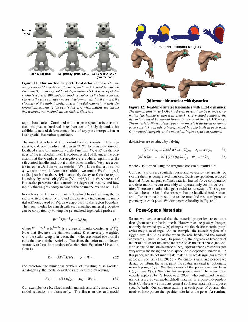
Figure 11: Our method supports local deformations. Our lo-calized basis (20 modes on the head, and r = 100 total for the en-tire model) produces good local deformations (c). A basis of globalmethods requires 180 modes to produce motion in the bear’s cheeks,whereas the ears still have no local deformations. Furthermore, theglobality of the global modes causes “modal ringing”: visible de-formations appear in the bear’s left arm when pulling the cheeks(b), whereas our method has no such artifact (c).

region boundaries. Combined with our pose-space basis construc-tion, this gives us hard real-time character soft-body dynamics thatexhibits localized deformations, free of any pose-interpolation orbasis spatial discontinuity artifacts.

The user first selects d ≥ 1 control handles (points or line seg-ments), to denote d individual regions D. We then compute smooth,localized scalar bi-harmonic weight functions Wi ∈ Rn on the ver-tices of the tetrahedral mesh [Jacobson et al. 2011], under the con-dition that the weight is non-negative everywhere, equals 1 at thei-th control handle, and is 0 at all the other handles. We place a ver-tex to region Di if the vertex weight in Wi is larger than a thresholdη ; we use η = 0.1. After thresholding, we remap Wi from [η ,1]to [0,1] such that the weights smoothly decay to 0 on the regionboundary, by introducing W′i = (Wi−η)κ/(1−η)κ , where κ > 0is a scalar parameter that controls the degree of locality and howrapidly the weights decay to zero at the boundary; we use κ = 1/2.

In each region Di, we compute a localized basis by fixing the tetmesh vertices outside of Di, and progressively increasing the mate-rial stiffness, based on W′i, as we approach to the region boundary.The linear modes for a mesh with such modified material propertiescan be computed by solving the generalized eigenvalue problem

W−T KW−1ϕi = λiMϕi, (31)

where W = W T ∈ R3n×3n is a diagonal matrix consisting of W′i.Note that Because the stiffness matrix K is inversely weightedwith the scalar weight function, the modes are biased towards theparts that have higher weights. Therefore, the deformation decayssmoothly to 0 on the boundary of each region. Equation 31 is equiv-alent to

Kyi = λiW T MWyi, ϕi =Wyi, (32)

and therefore the numerical problem of inverting W is avoided.Analogously, the modal derivatives are localized by solving

Kzi j =−(H : ϕi)y j, ψi j =Wzi j. (33)

Our examples use localized modal analysis and self-contact-awaremodel reduction simultaneously. The linear modes and modal

Figure 12: Real-time inverse kinematics with FEM dynamics:The human arm (4 rig DOFs) is driven in real-time by inverse kine-matics (IK handle is shown in green). Our method computes thedynamics caused by inertial forces, in hard real time (1,100 FPS).The material stiffness of the upper arm muscle is designed to vary ateach pose (a), and this is incorporated into the basis at each pose.Our method interpolates the materials in pose space at runtime.

derivatives are obtained by solving

(ZT KZ)yi = λi(ZTW T MWZ)yi, ϕi =WZyi, (34)

(ZT KZ)zi j =−ZT((H : ϕi)Zy j

), ψi j =WZzi j, (35)

where Z is formed using the weighted constraint matrix CW .

Our basis vectors are spatially sparse and we exploit the sparsity bystoring them as compressed matrices. Basis interpolation, reducedinternal force, tangent stiffness matrix, inertial force computationand deformation vector assembly all operate only on non-zero en-tries. There are no other changes needed to our system. The regionsare kept the same for all the poses pi, but the localized basis vectorsare different in each pose, due to the modified rest configurationgeometry in each pose. We demonstrate locality in Figure 11.

8 Pose-Space Materials

So far, we have assumed that the material properties are constantthroughout our tetrahedral mesh. However, as the pose p changes,not only the rest shape Φ(p) changes, but the elastic material prop-erties may also change. As an example, the muscle region of arigged arm should be stiffer when the arm bends and the musclecontracts (Figure 12, (a)). In principle, the degrees of freedom ofmaterial design for the artist are three-fold: material space (the spe-cific shape of the strain-space curve), spatial space (materials thatvary across the mesh) and pose-space (pose-dependent material). Inthis paper, we do not investigate material space design (for a recentapproach, see [Xu et al. 2015b]). We enable spatial and pose-spacedesign by letting the artist paint the spatial material E, optionallyin each pose, E(pi). We then construct the pose-dependent basisU(pi) using E(pi). We note that per-pose materials have been pre-viously explored by [Galoppo et al. 2009], who performed the sim-ulation using St.Venant-Kirchhoff material in a pose-independentbasis U, whereas we simulate general nonlinear materials in a pose-specific basis. Our cubature training at each pose, of course, alsoneeds to incorporate the specific material at the pose. At runtime,

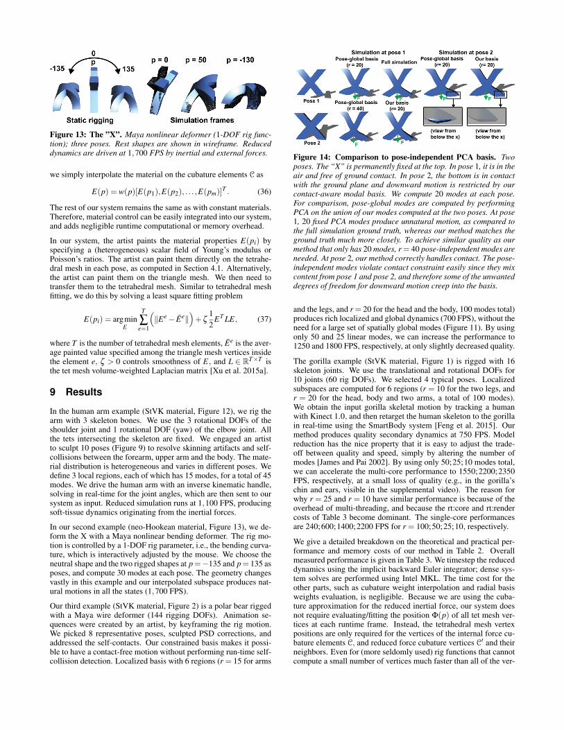
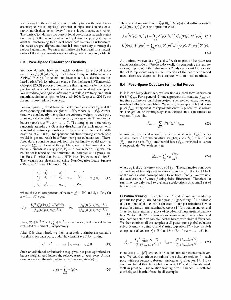
Figure 13: The ”X”. Maya nonlinear deformer (1-DOF rig func-tion); three poses. Rest shapes are shown in wireframe. Reduceddynamics are driven at 1,700 FPS by inertial and external forces.

we simply interpolate the material on the cubature elements C as

E(p) = w(p)[E(p1),E(p2), . . . ,E(pm)]T . (36)

The rest of our system remains the same as with constant materials.Therefore, material control can be easily integrated into our system,and adds negligible runtime computational or memory overhead.

In our system, the artist paints the material properties E(pi) byspecifying a (heterogeneous) scalar field of Young’s modulus orPoisson’s ratios. The artist can paint them directly on the tetrahe-dral mesh in each pose, as computed in Section 4.1. Alternatively,the artist can paint them on the triangle mesh. We then need totransfer them to the tetrahedral mesh. Similar to tetrahedral meshfitting, we do this by solving a least square fitting problem

E(pi) = argminE

T

∑e=1

(‖Ee− Ee‖

)+ζ

12

ET LE, (37)

where T is the number of tetrahedral mesh elements, Ee is the aver-age painted value specified among the triangle mesh vertices insidethe element e, ζ > 0 controls smoothness of E, and L ∈ RT×T isthe tet mesh volume-weighted Laplacian matrix [Xu et al. 2015a].

9 Results

In the human arm example (StVK material, Figure 12), we rig thearm with 3 skeleton bones. We use the 3 rotational DOFs of theshoulder joint and 1 rotational DOF (yaw) of the elbow joint. Allthe tets intersecting the skeleton are fixed. We engaged an artistto sculpt 10 poses (Figure 9) to resolve skinning artifacts and self-collisions between the forearm, upper arm and the body. The mate-rial distribution is heterogeneous and varies in different poses. Wedefine 3 local regions, each of which has 15 modes, for a total of 45modes. We drive the human arm with an inverse kinematic handle,solving in real-time for the joint angles, which are then sent to oursystem as input. Reduced simulation runs at 1,100 FPS, producingsoft-tissue dynamics originating from the inertial forces.

In our second example (neo-Hookean material, Figure 13), we de-form the X with a Maya nonlinear bending deformer. The rig mo-tion is controlled by a 1-DOF rig parameter, i.e., the bending curva-ture, which is interactively adjusted by the mouse. We choose theneutral shape and the two rigged shapes at p=−135 and p= 135 asposes, and compute 30 modes at each pose. The geometry changesvastly in this example and our interpolated subspace produces nat-ural motions in all the states (1,700 FPS).

Our third example (StVK material, Figure 2) is a polar bear riggedwith a Maya wire deformer (144 rigging DOFs). Animation se-quences were created by an artist, by keyframing the rig motion.We picked 8 representative poses, sculpted PSD corrections, andaddressed the self-contacts. Our constrained basis makes it possi-ble to have a contact-free motion without performing run-time self-collision detection. Localized basis with 6 regions (r = 15 for arms

Figure 14: Comparison to pose-independent PCA basis. Twoposes. The “X” is permanently fixed at the top. In pose 1, it is in theair and free of ground contact. In pose 2, the bottom is in contactwith the ground plane and downward motion is restricted by ourcontact-aware modal basis. We compute 20 modes at each pose.For comparison, pose-global modes are computed by performingPCA on the union of our modes computed at the two poses. At pose1, 20 fixed PCA modes produce unnatural motion, as compared tothe full simulation ground truth, whereas our method matches theground truth much more closely. To achieve similar quality as ourmethod that only has 20 modes, r = 40 pose-independent modes areneeded. At pose 2, our method correctly handles contact. The pose-independent modes violate contact constraint easily since they mixcontent from pose 1 and pose 2, and therefore some of the unwanteddegrees of freedom for downward motion creep into the basis.

and the legs, and r = 20 for the head and the body, 100 modes total)produces rich localized and global dynamics (700 FPS), without theneed for a large set of spatially global modes (Figure 11). By usingonly 50 and 25 linear modes, we can increase the performance to1250 and 1800 FPS, respectively, at only slightly decreased quality.

The gorilla example (StVK material, Figure 1) is rigged with 16skeleton joints. We use the translational and rotational DOFs for10 joints (60 rig DOFs). We selected 4 typical poses. Localizedsubspaces are computed for 6 regions (r = 10 for the two legs, andr = 20 for the head, body and two arms, a total of 100 modes).We obtain the input gorilla skeletal motion by tracking a humanwith Kinect 1.0, and then retarget the human skeleton to the gorillain real-time using the SmartBody system [Feng et al. 2015]. Ourmethod produces quality secondary dynamics at 750 FPS. Modelreduction has the nice property that it is easy to adjust the trade-off between quality and speed, simply by altering the number ofmodes [James and Pai 2002]. By using only 50;25;10 modes total,we can accelerate the multi-core performance to 1550;2200;2350FPS, respectively, at a small loss of quality (e.g., in the gorilla’schin and ears, visible in the supplemental video). The reason forwhy r = 25 and r = 10 have similar performance is because of theoverhead of multi-threading, and because the rt:core and rt:rendercosts of Table 3 become dominant. The single-core performancesare 240;600;1400;2200 FPS for r = 100;50;25;10, respectively.

We give a detailed breakdown on the theoretical and practical per-formance and memory costs of our method in Table 2. Overallmeasured performance is given in Table 3. We timestep the reduceddynamics using the implicit backward Euler integrator; dense sys-tem solves are performed using Intel MKL. The time cost for theother parts, such as cubature weight interpolation and radial basisweights evaluation, is negligible. Because we are using the cuba-ture approximation for the reduced inertial force, our system doesnot require evaluating/fitting the position Φ(p) of all tet mesh ver-tices at each runtime frame. Instead, the tetrahedral mesh vertexpositions are only required for the vertices of the internal force cu-bature elements C, and reduced force cubature vertices C′ and theirneighbors. Even for (more seldomly used) rig functions that cannotcompute a small number of vertices much faster than all of the ver-

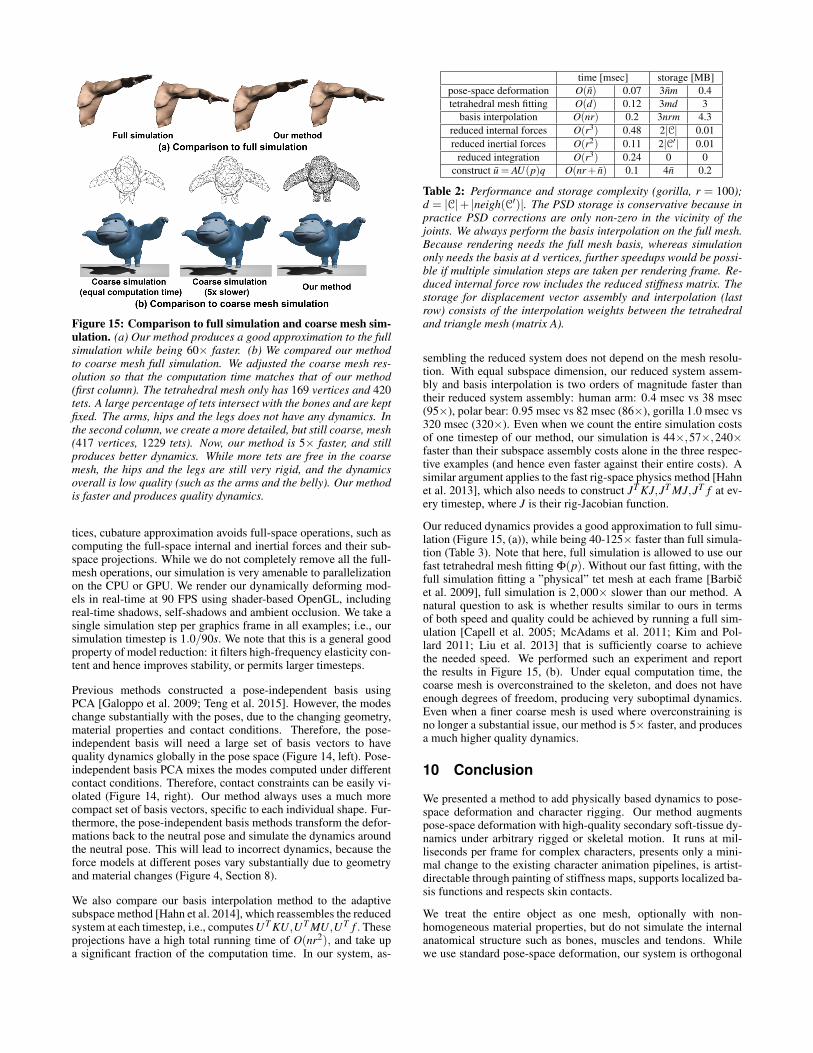
Figure 15: Comparison to full simulation and coarse mesh sim-ulation. (a) Our method produces a good approximation to the fullsimulation while being 60× faster. (b) We compared our methodto coarse mesh full simulation. We adjusted the coarse mesh res-olution so that the computation time matches that of our method(first column). The tetrahedral mesh only has 169 vertices and 420tets. A large percentage of tets intersect with the bones and are keptfixed. The arms, hips and the legs does not have any dynamics. Inthe second column, we create a more detailed, but still coarse, mesh(417 vertices, 1229 tets). Now, our method is 5× faster, and stillproduces better dynamics. While more tets are free in the coarsemesh, the hips and the legs are still very rigid, and the dynamicsoverall is low quality (such as the arms and the belly). Our methodis faster and produces quality dynamics.

tices, cubature approximation avoids full-space operations, such ascomputing the full-space internal and inertial forces and their sub-space projections. While we do not completely remove all the full-mesh operations, our simulation is very amenable to parallelizationon the CPU or GPU. We render our dynamically deforming mod-els in real-time at 90 FPS using shader-based OpenGL, includingreal-time shadows, self-shadows and ambient occlusion. We take asingle simulation step per graphics frame in all examples; i.e., oursimulation timestep is 1.0/90s. We note that this is a general goodproperty of model reduction: it filters high-frequency elasticity con-tent and hence improves stability, or permits larger timesteps.

Previous methods constructed a pose-independent basis usingPCA [Galoppo et al. 2009; Teng et al. 2015]. However, the modeschange substantially with the poses, due to the changing geometry,material properties and contact conditions. Therefore, the pose-independent basis will need a large set of basis vectors to havequality dynamics globally in the pose space (Figure 14, left). Pose-independent basis PCA mixes the modes computed under differentcontact conditions. Therefore, contact constraints can be easily vi-olated (Figure 14, right). Our method always uses a much morecompact set of basis vectors, specific to each individual shape. Fur-thermore, the pose-independent basis methods transform the defor-mations back to the neutral pose and simulate the dynamics aroundthe neutral pose. This will lead to incorrect dynamics, because theforce models at different poses vary substantially due to geometryand material changes (Figure 4, Section 8).

We also compare our basis interpolation method to the adaptivesubspace method [Hahn et al. 2014], which reassembles the reducedsystem at each timestep, i.e., computes UT KU,UT MU,UT f . Theseprojections have a high total running time of O(nr2), and take upa significant fraction of the computation time. In our system, as-

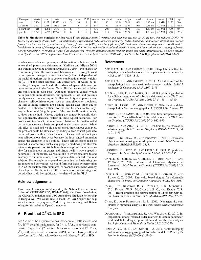
time [msec] storage [MB]pose-space deformation O(n) 0.07 3nm 0.4tetrahedral mesh fitting O(d) 0.12 3md 3

basis interpolation O(nr) 0.2 3nrm 4.3reduced internal forces O(r3) 0.48 2|C| 0.01reduced inertial forces O(r2) 0.11 2|C′| 0.01

reduced integration O(r3) 0.24 0 0construct u = AU(p)q O(nr+ n) 0.1 4n 0.2

Table 2: Performance and storage complexity (gorilla, r = 100);d = |C|+ |neigh(C′)|. The PSD storage is conservative because inpractice PSD corrections are only non-zero in the vicinity of thejoints. We always perform the basis interpolation on the full mesh.Because rendering needs the full mesh basis, whereas simulationonly needs the basis at d vertices, further speedups would be possi-ble if multiple simulation steps are taken per rendering frame. Re-duced internal force row includes the reduced stiffness matrix. Thestorage for displacement vector assembly and interpolation (lastrow) consists of the interpolation weights between the tetrahedraland triangle mesh (matrix A).

sembling the reduced system does not depend on the mesh resolu-tion. With equal subspace dimension, our reduced system assem-bly and basis interpolation is two orders of magnitude faster thantheir reduced system assembly: human arm: 0.4 msec vs 38 msec(95×), polar bear: 0.95 msec vs 82 msec (86×), gorilla 1.0 msec vs320 msec (320×). Even when we count the entire simulation costsof one timestep of our method, our simulation is 44×,57×,240×faster than their subspace assembly costs alone in the three respec-tive examples (and hence even faster against their entire costs). Asimilar argument applies to the fast rig-space physics method [Hahnet al. 2013], which also needs to construct JT KJ,JT MJ,JT f at ev-ery timestep, where J is their rig-Jacobian function.

Our reduced dynamics provides a good approximation to full simu-lation (Figure 15, (a)), while being 40-125× faster than full simula-tion (Table 3). Note that here, full simulation is allowed to use ourfast tetrahedral mesh fitting Φ(p). Without our fast fitting, with thefull simulation fitting a ”physical” tet mesh at each frame [Barbicet al. 2009], full simulation is 2,000× slower than our method. Anatural question to ask is whether results similar to ours in termsof both speed and quality could be achieved by running a full sim-ulation [Capell et al. 2005; McAdams et al. 2011; Kim and Pol-lard 2011; Liu et al. 2013] that is sufficiently coarse to achievethe needed speed. We performed such an experiment and reportthe results in Figure 15, (b). Under equal computation time, thecoarse mesh is overconstrained to the skeleton, and does not haveenough degrees of freedom, producing very suboptimal dynamics.Even when a finer coarse mesh is used where overconstraining isno longer a substantial issue, our method is 5× faster, and producesa much higher quality dynamics.

10 Conclusion

We presented a method to add physically based dynamics to pose-space deformation and character rigging. Our method augmentspose-space deformation with high-quality secondary soft-tissue dy-namics under arbitrary rigged or skeletal motion. It runs at mil-liseconds per frame for complex characters, presents only a mini-mal change to the existing character animation pipelines, is artist-directable through painting of stiffness maps, supports localized ba-sis functions and respects skin contacts.

We treat the entire object as one mesh, optionally with non-homogeneous material properties, but do not simulate the internalanatomical structure such as bones, muscles and tendons. Whilewe use standard pose-space deformation, our system is orthogonal

Example tet-vtx tet-el tri-vtx r reg poses PSD cub:int cub:inert rt:core rt:dyn rt:render rt:total mem FPS sparm 2364 8122 10525 45 3 10 9 192 45 36 % 58 % 6% 0.87 ms 11 MB 1150 60×X-shape 3077 9303 2362 30 1 3 0 144 50 26 % 65 % 9% 0.59 ms 4.2 MB 1700 105×polar bear 4018 12762 6876 100 6 8 7 336 200 29 % 66 % 5% 1.43 ms 7.3 MB 700 40×gorilla 3771 16297 15774 100 6 4 2 144 119 29 % 63 % 8% 1.33 ms 7.9 MB 750 125×

Table 3: Simulation statistics for #tet mesh Γ and triangle mesh Γ vertices and elements (tet-vtx, tet-el, tri-vtx), #of reduced DOFs (r),#local regions (reg), #poses with a simulation basis (poses) and PSD-corrected geometry (PSD), #cubature samples for internal and inertialforces (cub:int, cub:inert), total memory (mem), frame rate (FPS), speedup (sp) over full simulation, simulation step time (rt:total), and itsbreakdown in terms of timestepping reduced dynamics (rt:dyn: reduced internal and inertial forces, and integration), constructing deforma-tions for rendering (rt:render, u = AU(p)q), and the rest (rt:core; including sparse tet mesh fitting and basis interpolation). We use 8 threadswith OpenMP; no GPU computation. Intel Xeon 2.9 GHz CPU (2×8 cores; 32GB RAM); GeForce GTX 680 graphics card (2GB RAM).

to other more advanced pose-space deformation techniques, suchas weighted pose-space deformation [Kurihara and Miyata 2004]and weight-decay regularization [Anjyo et al. 2014]. For shapes farfrom training data, the normalized biharmonic RBF weights usedin our system converge to a constant value (a limit, independent ofthe radial direction) that is a convex combinations (with weightson [0,1]) of the artist-sculpted PSD corrections. It would be in-teresting to explore such and other advanced sparse data interpo-lation techniques in the future. Our collisions are treated as bilat-eral constraints in each pose. Although unilateral contact wouldbe in principle more desirable, our approach is fast, and preventsour dynamics from causing self-collisions. In typical poses wherecharacter self-collisions occur, such as bent elbows or shoulders,the self-colliding surfaces are pushing against each other due tocontact. It is therefore difficult for the skin to break contact any-way without modifying the pose. If the pose itself breaks contact,so does our method. Hence, treating the contact bilaterally doesnot significantly decrease realism in these typical scenarios. Forposes close to contact, the interpolated basis can be contaminatedby the contact-aware basis computed at the contact pose. Whilethis effect is small and we did not observe artifacts in our examples,the problem could be alleviated by adding a near-contact pose intothe set of poses with a reduced model. Our method does not pre-vent self-collisions that occur because the input rigged animationcauses the character to self-collide. These self-collisions must beavoided in another way, such as by properly modifying the skeletonjoints or rig parameters. We believe these compromises are reason-able for applications in games and virtual reality, where speed isparamount. In the future, we would like to investigate how to addanatomy to our simulations, or incorporate data scanned from realsubjects. For example, as opposed to computing the basis using lin-ear modes and derivatives, we could form our basis by performingPCA on the anatomically simulated, or scanned data, in the vicinityof each pose. We did not use GPU computation; several stages ofour pipeline could be significantly accelerated on the GPU.

Acknowledgements

This research was sponsored in part by the National Science Foun-dation (CAREER-1055035, IIS-1422869), the Sloan Foundation,the Okawa Foundation, and USC Annenberg Graduate Fellowshipto Hongyi Xu. We would like to thank Dr. Ari Shapiro for helpwith the SmartBody system, Carlos Joy for modeling, and BohanWang for his real-time OpenGL renderer.

A Proof that ZT AZ is SPD

Let A ∈ Rn×n be a symmetric positive-definite (SPD) matrix, andZ ∈Rn×k be a full-rank matrix, for k≤ n. ZT AZ is obviously sym-metric. Suppose xT (ZT AZ)x = 0 for some vector x ∈ Rk. Then,yT Ay = 0, for y = Zx. Because A is SPD, we must have y = 0, andtherefore, as Z is full-rank, we have x = 0. Hence, ZT AZ is SPD.

References

AMSALLEM, D., AND FARHAT, C. 2008. Interpolation method foradapting reduced-order models and application to aeroelasticity.AIAA J. 46, 7, 1803–1813.

AMSALLEM, D., AND FARHAT, C. 2011. An online method forinterpolating linear parametric reduced-order models. SIAM J.on Scientific Computing 33, 5, 2169–2198.

AN, S. S., KIM, T., AND JAMES, D. L. 2008. Optimizing cubaturefor efficient integration of subspace deformations. ACM Trans.on Graphics (SIGGRAPH Asia 2008) 27, 5, 165:1–165:10.

ANJYO, K., LEWIS, J. P., AND PIGHIN, F. 2014. Scattered datainterpolation for computer graphics. In SIGGRAPH Courses, 27.

BARBIC, J., AND JAMES, D. L. 2005. Real-time subspace integra-tion for St. Venant-Kirchhoff deformable models. ACM Trans.on Graphics (SIGGRAPH 2005) 24, 3, 982–990.

BARBIC, J., AND ZHAO, Y. 2011. Real-time large-deformationsubstructuring. ACM Trans. on Graphics (SIGGRAPH 2011) 30,4, 91:1–91:7.

BARBIC, J., DA SILVA, M., AND POPOVIC, J. 2009. Deformableobject animation using reduced optimal control. ACM Trans. onGraphics (SIGGRAPH 2009) 28, 3.

BARNHILL, R., DUBE, R., AND LITTLE, F. 1983. Properties ofShepards Surfaces. Rocky Mountain J. Math. 13, 365–382.

CAPELL, S., GREEN, S., CURLESS, B., DUCHAMP, T., ANDPOPOVIC, Z. 2002. Interactive skeleton-driven dynamic de-formations. ACM Trans. on Graphics (SIGGRAPH 2002) 21, 3,586–593.

CAPELL, S., BURKHART, M., CURLESS, B., DUCHAMP, T., ANDPOPOVIC, Z. 2005. Physically based rigging for deformablecharacters. In Symp. on Computer Animation (SCA), 301–310.

CARR, J. C., BEATSON, R. K., CHERRIE, J. B., MITCHELL,T. J., FRIGHT, W. R., MCCALLUM, B. C., AND EVANS, T. R.2001. Reconstruction and representation of 3d objects with ra-dial basis functions. In Proc. of ACM SIGGRAPH 2001, 67–76.

CHEN, D., AND PLEMMONS, R. J. 2006. Nonnegativity con-straints in numerical analysis. In Symp. on the Birth of NumericalAnalysis.

DEGROOTE, J., VIERENDEELS, J., AND WILLCOX, K. 2010. In-terpolation among reduced-order matrices to obtain parameter-ized models for design, optimization and probabilistic analysis.Int. J. for Numerical Methods in Fluids 63, 2, 207–230.

FENG, A., CASAS, D., AND SHAPIRO, A. 2015. Avatar reshapingand automatic rigging using a deformable model. In Proc. of theMotion in Games (MIG) Conf., 57–64.

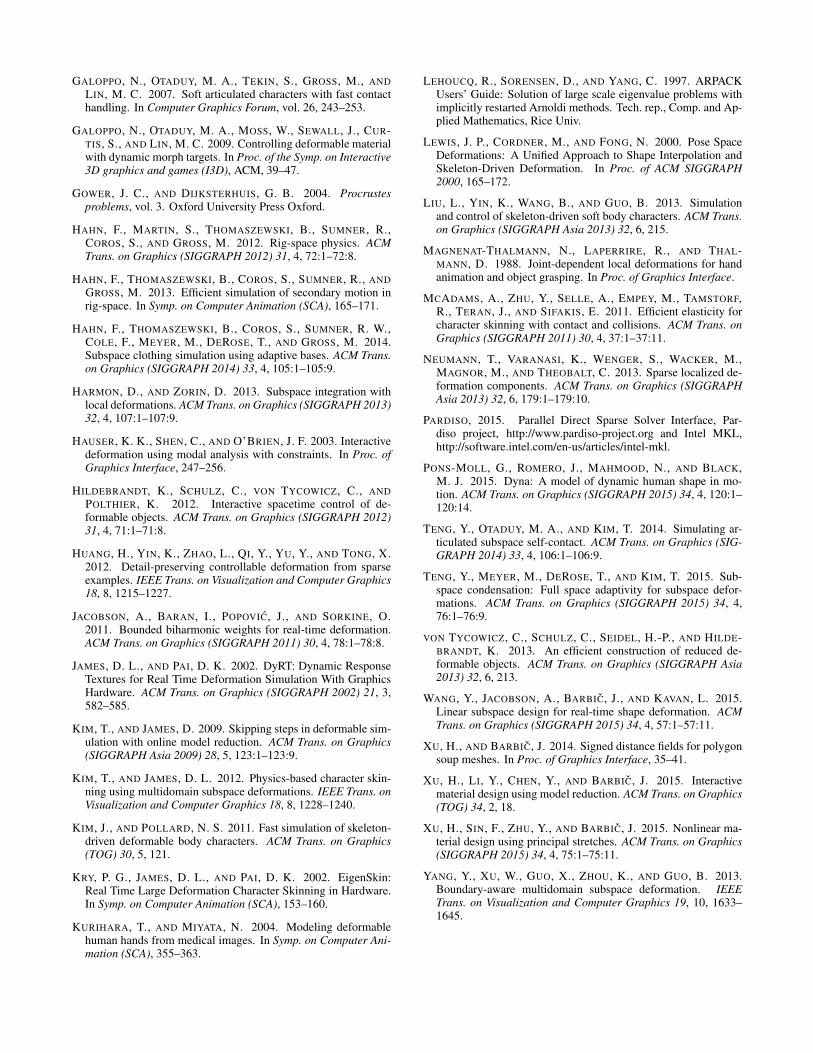
GALOPPO, N., OTADUY, M. A., TEKIN, S., GROSS, M., ANDLIN, M. C. 2007. Soft articulated characters with fast contacthandling. In Computer Graphics Forum, vol. 26, 243–253.

GALOPPO, N., OTADUY, M. A., MOSS, W., SEWALL, J., CUR-TIS, S., AND LIN, M. C. 2009. Controlling deformable materialwith dynamic morph targets. In Proc. of the Symp. on Interactive3D graphics and games (I3D), ACM, 39–47.

GOWER, J. C., AND DIJKSTERHUIS, G. B. 2004. Procrustesproblems, vol. 3. Oxford University Press Oxford.

HAHN, F., MARTIN, S., THOMASZEWSKI, B., SUMNER, R.,COROS, S., AND GROSS, M. 2012. Rig-space physics. ACMTrans. on Graphics (SIGGRAPH 2012) 31, 4, 72:1–72:8.

HAHN, F., THOMASZEWSKI, B., COROS, S., SUMNER, R., ANDGROSS, M. 2013. Efficient simulation of secondary motion inrig-space. In Symp. on Computer Animation (SCA), 165–171.

HAHN, F., THOMASZEWSKI, B., COROS, S., SUMNER, R. W.,COLE, F., MEYER, M., DEROSE, T., AND GROSS, M. 2014.Subspace clothing simulation using adaptive bases. ACM Trans.on Graphics (SIGGRAPH 2014) 33, 4, 105:1–105:9.

HARMON, D., AND ZORIN, D. 2013. Subspace integration withlocal deformations. ACM Trans. on Graphics (SIGGRAPH 2013)32, 4, 107:1–107:9.

HAUSER, K. K., SHEN, C., AND O’BRIEN, J. F. 2003. Interactivedeformation using modal analysis with constraints. In Proc. ofGraphics Interface, 247–256.

HILDEBRANDT, K., SCHULZ, C., VON TYCOWICZ, C., ANDPOLTHIER, K. 2012. Interactive spacetime control of de-formable objects. ACM Trans. on Graphics (SIGGRAPH 2012)31, 4, 71:1–71:8.

HUANG, H., YIN, K., ZHAO, L., QI, Y., YU, Y., AND TONG, X.2012. Detail-preserving controllable deformation from sparseexamples. IEEE Trans. on Visualization and Computer Graphics18, 8, 1215–1227.

JACOBSON, A., BARAN, I., POPOVIC, J., AND SORKINE, O.2011. Bounded biharmonic weights for real-time deformation.ACM Trans. on Graphics (SIGGRAPH 2011) 30, 4, 78:1–78:8.

JAMES, D. L., AND PAI, D. K. 2002. DyRT: Dynamic ResponseTextures for Real Time Deformation Simulation With GraphicsHardware. ACM Trans. on Graphics (SIGGRAPH 2002) 21, 3,582–585.

KIM, T., AND JAMES, D. 2009. Skipping steps in deformable sim-ulation with online model reduction. ACM Trans. on Graphics(SIGGRAPH Asia 2009) 28, 5, 123:1–123:9.

KIM, T., AND JAMES, D. L. 2012. Physics-based character skin-ning using multidomain subspace deformations. IEEE Trans. onVisualization and Computer Graphics 18, 8, 1228–1240.

KIM, J., AND POLLARD, N. S. 2011. Fast simulation of skeleton-driven deformable body characters. ACM Trans. on Graphics(TOG) 30, 5, 121.

KRY, P. G., JAMES, D. L., AND PAI, D. K. 2002. EigenSkin:Real Time Large Deformation Character Skinning in Hardware.In Symp. on Computer Animation (SCA), 153–160.

KURIHARA, T., AND MIYATA, N. 2004. Modeling deformablehuman hands from medical images. In Symp. on Computer Ani-mation (SCA), 355–363.

LEHOUCQ, R., SORENSEN, D., AND YANG, C. 1997. ARPACKUsers’ Guide: Solution of large scale eigenvalue problems withimplicitly restarted Arnoldi methods. Tech. rep., Comp. and Ap-plied Mathematics, Rice Univ.

LEWIS, J. P., CORDNER, M., AND FONG, N. 2000. Pose SpaceDeformations: A Unified Approach to Shape Interpolation andSkeleton-Driven Deformation. In Proc. of ACM SIGGRAPH2000, 165–172.

LIU, L., YIN, K., WANG, B., AND GUO, B. 2013. Simulationand control of skeleton-driven soft body characters. ACM Trans.on Graphics (SIGGRAPH Asia 2013) 32, 6, 215.

MAGNENAT-THALMANN, N., LAPERRIRE, R., AND THAL-MANN, D. 1988. Joint-dependent local deformations for handanimation and object grasping. In Proc. of Graphics Interface.

MCADAMS, A., ZHU, Y., SELLE, A., EMPEY, M., TAMSTORF,R., TERAN, J., AND SIFAKIS, E. 2011. Efficient elasticity forcharacter skinning with contact and collisions. ACM Trans. onGraphics (SIGGRAPH 2011) 30, 4, 37:1–37:11.

NEUMANN, T., VARANASI, K., WENGER, S., WACKER, M.,MAGNOR, M., AND THEOBALT, C. 2013. Sparse localized de-formation components. ACM Trans. on Graphics (SIGGRAPHAsia 2013) 32, 6, 179:1–179:10.

PARDISO, 2015. Parallel Direct Sparse Solver Interface, Par-diso project, http://www.pardiso-project.org and Intel MKL,http://software.intel.com/en-us/articles/intel-mkl.

PONS-MOLL, G., ROMERO, J., MAHMOOD, N., AND BLACK,M. J. 2015. Dyna: A model of dynamic human shape in mo-tion. ACM Trans. on Graphics (SIGGRAPH 2015) 34, 4, 120:1–120:14.

TENG, Y., OTADUY, M. A., AND KIM, T. 2014. Simulating ar-ticulated subspace self-contact. ACM Trans. on Graphics (SIG-GRAPH 2014) 33, 4, 106:1–106:9.

TENG, Y., MEYER, M., DEROSE, T., AND KIM, T. 2015. Sub-space condensation: Full space adaptivity for subspace defor-mations. ACM Trans. on Graphics (SIGGRAPH 2015) 34, 4,76:1–76:9.

VON TYCOWICZ, C., SCHULZ, C., SEIDEL, H.-P., AND HILDE-BRANDT, K. 2013. An efficient construction of reduced de-formable objects. ACM Trans. on Graphics (SIGGRAPH Asia2013) 32, 6, 213.

WANG, Y., JACOBSON, A., BARBIC, J., AND KAVAN, L. 2015.Linear subspace design for real-time shape deformation. ACMTrans. on Graphics (SIGGRAPH 2015) 34, 4, 57:1–57:11.

XU, H., AND BARBIC, J. 2014. Signed distance fields for polygonsoup meshes. In Proc. of Graphics Interface, 35–41.

XU, H., LI, Y., CHEN, Y., AND BARBIC, J. 2015. Interactivematerial design using model reduction. ACM Trans. on Graphics(TOG) 34, 2, 18.

XU, H., SIN, F., ZHU, Y., AND BARBIC, J. 2015. Nonlinear ma-terial design using principal stretches. ACM Trans. on Graphics(SIGGRAPH 2015) 34, 4, 75:1–75:11.

YANG, Y., XU, W., GUO, X., ZHOU, K., AND GUO, B. 2013.Boundary-aware multidomain subspace deformation. IEEETrans. on Visualization and Computer Graphics 19, 10, 1633–1645.