Portfolio Theory

Moty Katzman

September 19, 2014

Portfolio Theory

Aim: To find optimal investment strategies.

Investors’ preferences:

How does a person decide which investment is best?Is “Best”=“highest expected return”?

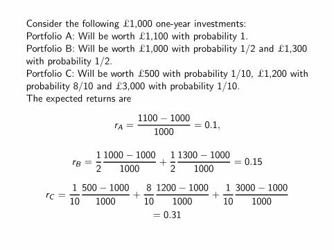
Consider the following £1,000 one-year investments:Portfolio A: Will be worth £1,100 with probability 1.Portfolio B: Will be worth £1,000 with probability 1/2 and £1,300with probability 1/2.Portfolio C: Will be worth £500 with probability 1/10, £1,200 withprobability 8/10 and £3,000 with probability 1/10.The expected returns are

rA =1100 − 1000

1000= 0.1,

rB =1

2

1000 − 1000

1000+

1

2

1300 − 1000

1000= 0.15

rC =1

10

500− 1000

1000+

8

10

1200 − 1000

1000+

1

10

3000 − 1000

1000

= 0.31

Now consider the following investors:Mr. X: Wants to sail around the world on a cruise costing £1,200 ayear from now.Ms. Y: Must repay her mortgage in a year and must have £1,100to do so.Dr. Z: Needs to buy a rare book worth £1,300.The chances of Mr X. sailing around the world if he invests ininvestments A,B or C are 0, 1/2 and 9/10 respectively, so heshould be advised to invest in C.Only investment A guarantees a return sufficient for Ms. Y to payher mortgage and she should choose it.The probability of the investments being worth at least £1,300after a year are 0, 1/2 and 1/10 respectively, so Dr. Z shouldinvest in portfolio B.

So different investors prefer different investments!“highest expected returns”6=“optimal”: the whole distribution ofthe returns needs to be taken into account.Instead of considering the whole distribution of the returns of aninvestment we take into account two parameters:the expected return which we denote r and thestandard deviation of the return which we denote σ.We now rephrase our problem: given a set of investments whosereturns have known expected values and standard deviations,which one is “optimal”?

Axioms satisfied by preferences

Consider two investments A and B with expected returns rA and rBand standard deviation of returns σA and σB .The following assumptions look plausible:A1 Investors are greedy:

If σA = σB and rA > rB investors prefer A to B.A2 Investors are risk averse:

If rA = rB and σA > σB investors prefer B to A.A3 Transitivity of preferences:

If investment B is preferable to A and if investment C is preferableto B then investment C is preferable to A.

We are introducing a partial ordering ≺ on the points of the σ-rplane:

r

σ

A(σA, rA)

B(σB , rB ) C(σC , rC )

D(σD , rD)

B is preferable to both A and C. Investments A and C areincomparable.

Indifference curves

We describe the preferences of an investor by specifying the sets ofinvestments which are equally attractive to the given investor.We define an indifference curve of an investor: this is the curveconsisting of points (σ, r) for which investments with theseexpected returns and standard deviation of returns are all equallyattractive to our investor.Notice that assumptions A1, A2 and A3 imply that these curvesmust be non-decreasing. (Why?)

Consider hypothetical investors X,Y,Z and W with the followingindifference curves.

r

σInvestor X

Investor X cannot tolerate uncertainty at all: this investorprefers a certain zero return rather a very large expectedreturn with a small degree of uncertainty.

r

σInvestor Y

Investor Y is willing to take some risks

r

σInvestor Z

but not as much as investor Z(his indifference curves are steeper.)

r

σInvestor W

Investor W is risk neutral.

Portfolios consisting entirely of risky investments

Consider two investments A and B with expected returns rA and rBand standard deviation of returns σA and σB .We split an investment of £1 between the two investments:consider portfolio Πt consisting of t units of investment A and1− t units of investment B.

We can do this for any t and not just 0 ≤ t ≤ 1.For example, to construct portfolio Π2 we short sell £1 worth of Band buy £2 worth of A, for a total investment of £1.

Let A and B be the random variables representing the annualreturn of investments A and B.The variance of Πt is given by Var(Πt) = Var(tA+ (1− t)B)= Var(tA) + Var((1− t)B) + 2Covar(tA, (1 − t)B)= t2Var(A) + (1− t)2Var(B) + 2t(1− t)Covar(A,B)= t2Var(A) + (1− t)2Var(B)+ 2t(1− t)ρ(A,B)

√

Var(A)Var(B)= (tσA)

2 + 2t(1− t)ρ(A,B)σAσB + ((1 − t)σB)2

The shapes of these curves are concave:Proposition 7.1: The curve in the σ-r plane given parametricallyby

(√

(tσA)2 + 2t(1− t)ρ(A,B)σAσB + ((1 − t)σB)2,trA + (1− t)rB

)

for 0 ≤ t ≤ 1 lies to the left of the line segmentconnecting the points (σA, rA) and (σB , rB).Proof: Since ρ(A,B) ≤ 1,√

(tσA)2 + 2t(1− t)ρ(A,B)σAσB + ((1− t)σB)2

≤√

(tσA)2 + 2t(1− t)σAσB + ((1 − t)σB)2

=

√

(tσA + (1− t)σB)2 = tσA + (1− t)σB .

The result follows from the fact that the parametric equation ofthe line segment connecting the points (σA, rA) and (σB , rB) is

{(tσA + (1− t)σB , trA + (1− t)rB) | 0 ≤ t ≤ 1} .

The feasible set

Suppose now that there are many different investments A1, . . . ,An

available.We can invest our one unit of currency by investing ti in Ai foreach 1 ≤ i ≤ n as long as

∑

n

i=1 ti = 1.What are all possible pairs (σ, r) corresponding to these portfolios?This set of points in the σ-r plane is called the feasible set.

Feasible sets

σ

r

Efficient portfolios

Which portfolios among all possible ones should an investor

satisfying axioms A1,A2 and A3 choose?

Definition:

An efficient portfolio is a feasible portfolio that provides thegreatest expected return for a given level of risk, or equivalently,the lowest risk for a given expected return. This is also called anoptimal portfolio. The efficient frontier is the set of all efficientportfolios. Obviously, our investor should choose a portfolio alongthe efficient frontier!

Feasible sets are convex along efficient frontier:

σ

r

A

B

The feasible set is convex along the efficient frontier, in the sensethat for any two portfolios A and B in the feasible set, there existfeasible portfolios above the portfolios in the segment connectingA and B.

Which efficient portfolio do we choose?

σ

r

But which portfolio along the efficient frontier will our investorchoose?This is where risk preferences start playing a role.

Different choices of portfolios for different appetites for risk

Consider investors X (with no risk tolerance at all) and W (riskneutral) discussed before together with investor U whoseindifference curves are given below.

σ

r

X

U

W

Optimal portfolios occur where indifference curves are

tangent to the efficient frontier.

If the indifference curves are not too badly behaved, e.g., if theindifference curves are the level curves of some smooth functionF (σ, r), then we should expect the optimal portfolio to be at apoint where the indifference curve is tangent to the efficientfrontier.Otherwise, if it occurs at a point where the indifference curveintersects the efficient frontier transversally, find an almost parallelindifference curve very close to the original one and to its left.

σ

r

A better portfolio!

A good portfolio.

Portfolios on this curve are more desirable and,if we chose the second indifference curve closeenough to the original one, it will also intersectthe efficient frontier, and this intersection willcorrespond to a better choice of portfolio thanthe one corresponding to the original point ofintersection.

Portfolios containing risk-free investments

We now add a risk-free investment B. Let rB be its (expected)return. Since rB is constant, its covariance with the returns of anyother portfolio Π is zero so the portfolio Πt consisting of t units ofcurrency invested in B and (1− t) units of currency invested in Πhas expected return

E (tB + (1− t)Π) = trB + (1− t)rΠ

(where we used B and Π to denote also the returns of theinvestments B and Π) and standard deviation of return√

Var(tB + (1− t)Π) =√

Var((1 − t)Π)

=√

(1− t)2Var(Π) = |1− t|σΠ.

The curve t 7→ (σΠt, rΠt

) for t ≤ 1 is a straight line passingthrough the points (0, rB ) and (σΠ, rΠ) and all the points on orbelow such a line will be part of the feasible set.What happens to the efficient frontier? Consider the set Sconsisting of all the slopes s of lines ℓs in the σ-r plane which passthrough the point (0, rB) and intersect the feasible set. Let m bethe supremum of S . Consider now the line ℓm which is above allthe others:

The line ℓm will either be tangent to the efficient frontier orasymptotic to it.We will see in Chapter 8 that, if we impose additional conditionson markets and investors, ℓm cannot be an asymptote of theefficient frontier and so it is tangent to it.

σ

r

Market Portfolio

This point of tangency is called the mar-

ket portfolio and we shall denote the cor-responding portfolio with M.The new efficient frontier, ℓm is calledthe capital market line.

We just proved the following:Theorem 7.2:

In the presence of a risk-free investment there exists an(essentially) unique investment choice consisting entirely of riskyinvestments which is efficient, namely, the market portfolio.Any other efficient investment is a combination of an investment inthe market portfolio and in the risk-free investment.

The End